����������������� ������������� �� ������

About this manual – Please read first ImageJ is a public domain Java image processing program inspired by NIH Image for the Macintosh. It runs on any computer with a Java 1.1 or later virtual machine, either as an online applet or as a downloadable application. The author, Wayne Rasband (wayne@codon.nih.gov), is at the Research Services Branch, National Institute of Mental Health, Bethesda, Maryland, USA.

The best source of information about ImageJ can be found at the ImageJ homepage (http://rsb.info.nih.gov/ij/) and by subscribing to the ImageJ mailing list (details on the home page). This manual is meant to be an introduction to ImageJ for light microscopy – a small part of ImageJ’s repertoire.

ImageJ has a large number of native functions supplemented by an ever increasing number of “plugins” (optional extras needing installation). The core functions are described in detail on the ImageJ web site (follow the Documentations link). A plugin is a file (named *.class) which needs to be in the “plugins” sub-folder of the ImageJ folder, otherwise ImageJ will not load it.

In this manual, the native functions are referred to in italicised, black text, the plugins by italicised, dark-blue text. ImageJ functions can be accessed by keyboard shortcuts, or “hotkeys”. Some hotkeys are hard-wired in to ImageJ, while others are user-defined. Unlike most other Windows applications, keyboard shortcuts do not require the “control” key to be pressed (for example, in Microsoft Word, the hotkey to “copy” is Ctrl+C); in ImageJ, it is just “C”. Unless you have installed ImageJ from the Wright Cell Imaging Facility website (Manuals and Software link), the plugins referred to in this manual and some of customised the keyboard shortcuts (the “hotkeys”) may not work.

This collection of plugins has merely been collated and organised by me; they have all have been obtained free from the ImageJ website or elsewhere on the Internet. The credit for this work should go to the authors of the plugins (See Appendix). Please ensure that they are properly acknowledged in any publication that their work facilitates. I have attempted to include appropriate citations or contact details for each author. Let me know of any omissions and I will correct them immediately.

If you are a plugin author and you are not happy with the way your plugin is included or described or cited, please let me know. I will update this manual as necessary.

This manual is intended to be an introductory overview to get you up and running, and as such, is not exhaustive. I began working on this manual while employed at the Babraham Institute, Cambridge, UK (address below). I consider it now to be a “work in progress”. Please send any comments to:

Tony Collins, Ph.D. Facility Manager

Wright Cell Imaging Facility Toronto Western Research Institute

MC 13-407 399 Bathurst Street

Toronto, ON, M5T 2S8

Email: tonyc@uhnres.utoronto.ca Website: www.uhnresearch.ca/wcif

Table of Contents 1 Installing ImageJ .................................. ..........................................................................................1

1.1 Windows ............................................ ....................................................................................................... 1 1.1.1 Install program files............................................................................................................................................ 1 1.1.2 Update core program ......................................................................................................................................... 1 1.1.3 Set memory allocation ....................................................................................................................................... 1

1.2 Mac and Linux ...................................... .................................................................................................... 1 1.3 OS2 ............................................................................................................................................................ 1 1.4 QuickTime functionality............................ ............................................................................................... 1 1.5 Upgrading .......................................... ....................................................................................................... 1

1.5.1 ImageJ core program......................................................................................................................................... 1 1.5.2 Plugins............................................................................................................................................................... 2

1.6 Java Runtime Environment ........................... .......................................................................................... 2 1.6.1 About ................................................................................................................................................................. 2 1.6.2 JRE version comparison .................................................................................................................................... 2 1.6.3 Installation of JRE.............................................................................................................................................. 2 1.6.4 Compiling ImageJ plugins with a new JRE......................................................................................................... 3

2 Importing Image Files .............................. ......................................................................................4 2.1 Importing Zeiss LSM files.......................... .............................................................................................. 4 2.2 Importing Noran SGI file ........................... ............................................................................................... 4 2.3 Importing Biorad PIC files ......................... .............................................................................................. 4 2.4 Importing multiple files from folder............... ......................................................................................... 4 2.5 Importing Multi-RAW sequence from folder ........... ............................................................................... 5 2.6 Importing AVI and MOV files ........................ ........................................................................................... 5 2.7 Other Import functions ............................. ............................................................................................... 5

3 Saving and Exporting Files ......................... ..................................................................................6 4 Intensity vs Time analysis ......................... ....................................................................................7

4.1 Brightness and Contrast ............................ ............................................................................................. 7 4.2 Getting intensity values from single ROI ........... .................................................................................... 7 4.3 Dynamic intensity vs Time analysis................. ....................................................................................... 7 4.4 Getting intensity values from multiple ROIs ........ .................................................................................. 8 4.5 Obtaining timestamp data ........................... ............................................................................................ 9

4.5.1 Zeiss LSM.......................................................................................................................................................... 9 4.5.2 Noran................................................................................................................................................................. 9 4.5.3 Biorad ................................................................................................................................................................ 9

4.6 Pseudo-linescan.................................... ................................................................................................... 9 5 Particle Analysis .................................. .........................................................................................10

5.1 Automatic Particle counting........................ .......................................................................................... 10 5.1.1 Threshold segmentation................................................................................................................................... 10 5.1.2 Watershed segmentation ................................................................................................................................. 11 5.1.3 Analyse Particles ............................................................................................................................................. 11 5.1.4 Particle tracking ............................................................................................................................................... 11

5.2 Manual Counting .................................... ................................................................................................ 12 5.2.1 Cell Counter ..................................................................................................................................................... 12 5.2.2 Point Picker...................................................................................................................................................... 12

6 Colour analysis .................................... .........................................................................................13 6.1 Fluorescence Colocalisation Analysis ............... .................................................................................. 13

6.1.1 Colocalisation Coefficients ............................................................................................................................... 13 6.1.2 Highlighting colocalised pixels.......................................................................................................................... 14

7 Image intensity Processing ......................... ................................................................................15 7.1 Brightness and Contrast ............................ ........................................................................................... 15 7.2 Non-linear contrast stretch ........................ ........................................................................................... 15 7.3 Gamma .............................................. ...................................................................................................... 16 7.4 Filtering .......................................... ......................................................................................................... 17 7.5 Background correction.............................. ............................................................................................ 18 7.6 Flat-field correction.............................. .................................................................................................. 19

7.6.1 Proper correction ............................................................................................................................................. 19 7.6.2 Pseudo-correction............................................................................................................................................ 19

7.7 Masking unwanted regions ........................... ........................................................................................ 20 7.7.1 Simple masking ............................................................................................................................................... 20 7.7.2 Complex masking ............................................................................................................................................ 20

ii

8 Colour Image processing ............................ ................................................................................21 8.1 Merging multi-channel images....................... ....................................................................................... 21

8.1.1 Zeiss LSM multi-channel experiments.............................................................................................................. 21 8.1.2 Biorad multi-channel experiments .................................................................................................................... 21 8.1.3 Interleaved multi-channel experiments ............................................................................................................. 21 8.1.4 Colour merging ................................................................................................................................................ 22

8.2 Pseudocolour ....................................... .................................................................................................. 22 9 Stack-slice manipulations .......................... .................................................................................24

9.1 Slice shuffling/removing/Adding .................... ...................................................................................... 24 9.2 Stack dimension manipulations ...................... ..................................................................................... 25

10 z-Functions ........................................ ...........................................................................................26 10.1 Stack-Projections .................................. ................................................................................................. 26

10.1.1 Maximum intensity Z-projection:....................................................................................................................... 26 10.1.2 Sobel filter based Focussing ............................................................................................................................ 26 10.1.3 Wavelet-transform based focussing ................................................................................................................. 26

10.2 Volume render ...................................... .................................................................................................. 27 10.3 Surface Render..................................... .................................................................................................. 27 10.4 Axial-sectioning................................... ................................................................................................... 28 10.5 Orthogonal views ................................... ................................................................................................ 28 10.6 Stereo Pairs and Anaglyphs......................... ......................................................................................... 29

10.6.1 Volume rendered-anaglyphs ............................................................................................................................ 29 10.6.2 Surface rendered-anaglyphs ............................................................................................................................ 30

11 t-Functions ........................................ ............................................................................................31 11.1 Correcting for bleaching........................... ............................................................................................. 31 11.2 F÷F0......................................................................................................................................................... 32 11.3 Delta-F ............................................ ......................................................................................................... 33 11.4 Surface plotting ................................... ................................................................................................... 34

11.4.1 “Analyze/Surface plot” settings......................................................................................................................... 34 11.4.2 SurfaceJ settings ............................................................................................................................................. 34

12 Annotating images .................................. .....................................................................................35 12.1 Scale bar .......................................... ....................................................................................................... 35

12.1.1 Spatial calibration............................................................................................................................................. 35 12.1.2 Adding scale-bar .............................................................................................................................................. 35

12.2 Text and lines ..................................... .................................................................................................... 36 12.2.1 Issues with adding text..................................................................................................................................... 36 12.2.2 Adding Text/Line/Box ....................................................................................................................................... 36 12.2.3 Adding timestamps .......................................................................................................................................... 37 12.2.4 Adding event marker to movie.......................................................................................................................... 37

13 Appendix 1: Plugin Authors ......................... ...............................................................................38 14 Appendix II: Citing ImageJ and Plugins ............. ........................................................................40

14.1 ImageJ............................................. ........................................................................................................ 40 14.2 VolumeJ ............................................ ...................................................................................................... 40 14.3 TransformJ......................................... ..................................................................................................... 40 14.4 Extended Focus..................................... ................................................................................................. 40

15 Appendix III:I Plugins menu and sub-menus.......... ...................................................................41 16 Appendix IV: Cut out keyboard toolbar.............. ........................................................................42

1 INSTALLING IMAGEJ

1.1 Windows If you already have ImageJ installed, it may be worthwhile uninstalling it (rename the folder) and following the installation instructions below. This will match your copy of ImageJ to this manual. Extra plugins can be easily added later.

1.1.1 Install program files 1. Download the WCIF_Imagej_setup.exe file from the Wright Cell Imaging Facility’s website

(http://www.uhnresearch.ca/wcif). Follow the Downloads link. 2. Run the program. 3. A shortcut will be installed on your desktop and in your Start menu.

1.1.2 Update core program Now upgrade the ImageJ core program (file IJ.JAR) immediately from the ImageJ web site (See Section 1.5.1 below) – due to the frequency of upgrades, the version in the setup will be out of date. Get in to the habit of doing this routinely.

1.1.3 Set memory allocation Unlike other Windows applications ImageJ will only use the memory allocated to it. By default the WCIF ImageJ installation assumes a PC with 512Mb RAM, so ImageJ has been allocated 380 Mb by default (a recommended 75% of the total 512Mb). If your PC does not have 512Mb of RAM then change the allocated memory to equal 75% of total RAM via the menu command: “Edit/Options/Memory”. Specifying more than 75% of real RAM results in virtual RAM being used causing ImageJ to become very slow and unstable. See http://rsb.info.nih.gov/ij/docs/install/.

1.2 Mac and Linux The WCIF ImageJ installation is for Windows. Mac and Linux users can download ImageJ from http://rsb.info.nih.gov/ij/download.html and then install the WCIF “plugins-only” package. This will install the plugins detailed in this manual and the “preferences file” (IJ_PREFS.TXT), which will match the menu locations of the plugins and their shortcuts to this manual.

1.3 OS2 ImageJ will run on OS2; however, for Biorad users running OS2, ImageJ installation is complicated by the 8.3 filename limitation required by the LaserSharp software. Contact me (email tonyc) for help with this.

1.4 QuickTime functionality When QuickTime is installed with its default settings, Java functionality is not installed with it; this renders the QuickTime functions of ImageJ non-functional. QuickTime needs to be installed with a custom installation, with the QuickTime for Java option checked. This option is unchecked by default and is some way down the installation options list, so keep scrolling until you find it. This requires you to be logged in with “administrative privileges”. See http://rsb.info.nih.gov/ij/plugins/qt-install.html.

1.5 Upgrading 1.5.1 ImageJ core program

You do not need to be logged in as an administrator to do this, but ImageJ must be closed. ImageJ upgrades are very frequent, and major bugs addressed within days so ImageJ itself should be upgraded routinely. You can check your version of ImageJ by either noting the version that appears below the toolbar at start up, or by finding the version at the bottom of the ImageJ property list which can be called via the menu command “Plugins/Utilities/ImageJ properties…”. The latest version of ImageJ is available at: http://rsb.info.nih.gov/ij/upgrade/.

2

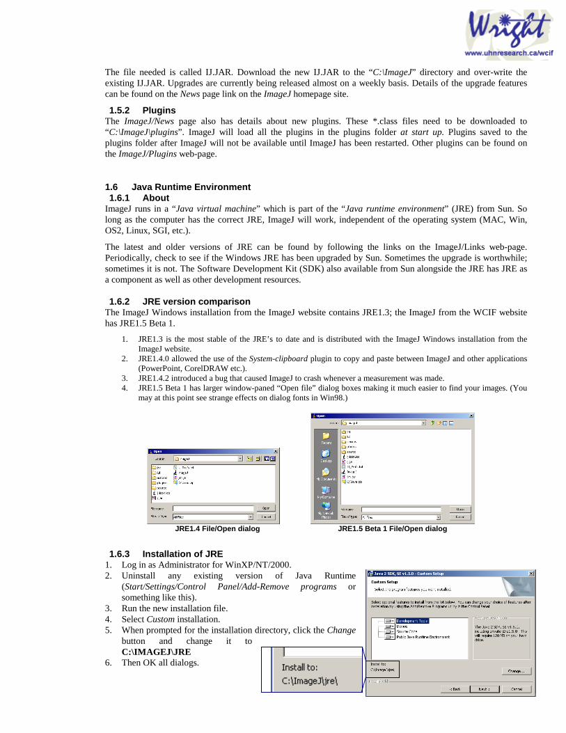
The file needed is called IJ.JAR. Download the new IJ.JAR to the “C:\ImageJ” directory and over-write the existing IJ.JAR. Upgrades are currently being released almost on a weekly basis. Details of the upgrade features can be found on the News page link on the ImageJ homepage site.

1.5.2 Plugins The ImageJ/News page also has details about new plugins. These *.class files need to be downloaded to “C:\ImageJ\plugins”. ImageJ will load all the plugins in the plugins folder at start up. Plugins saved to the plugins folder after ImageJ will not be available until ImageJ has been restarted. Other plugins can be found on the ImageJ/Plugins web-page.

1.6 Java Runtime Environment 1.6.1 About

ImageJ runs in a “Java virtual machine” which is part of the “Java runtime environment” (JRE) from Sun. So long as the computer has the correct JRE, ImageJ will work, independent of the operating system (MAC, Win, OS2, Linux, SGI, etc.).

The latest and older versions of JRE can be found by following the links on the ImageJ/Links web-page. Periodically, check to see if the Windows JRE has been upgraded by Sun. Sometimes the upgrade is worthwhile; sometimes it is not. The Software Development Kit (SDK) also available from Sun alongside the JRE has JRE as a component as well as other development resources.

1.6.2 JRE version comparison The ImageJ Windows installation from the ImageJ website contains JRE1.3; the ImageJ from the WCIF website has JRE1.5 Beta 1.

1. JRE1.3 is the most stable of the JRE’s to date and is distributed with the ImageJ Windows installation from the ImageJ website.

2. JRE1.4.0 allowed the use of the System-clipboard plugin to copy and paste between ImageJ and other applications (PowerPoint, CorelDRAW etc.).

3. JRE1.4.2 introduced a bug that caused ImageJ to crash whenever a measurement was made. 4. JRE1.5 Beta 1 has larger window-paned “Open file” dialog boxes making it much easier to find your images. (You

may at this point see strange effects on dialog fonts in Win98.)

JRE1.4 File/Open dialog JRE1.5 Beta 1 File/Open dialog

1.6.3 Installation of JRE 1. Log in as Administrator for WinXP/NT/2000. 2. Uninstall any existing version of Java Runtime

(Start/Settings/Control Panel/Add-Remove programs or something like this).

3. Run the new installation file. 4. Select Custom installation. 5. When prompted for the installation directory, click the Change

button and change it to C:\IMAGEJ\JRE

6. Then OK all dialogs.

3

Installing SDK rather than JRE will mean that javaw.exe will not be in the expected place. You need move the contents of the JRE folder installed by JDK to C:\IMAGEJ\JRE.

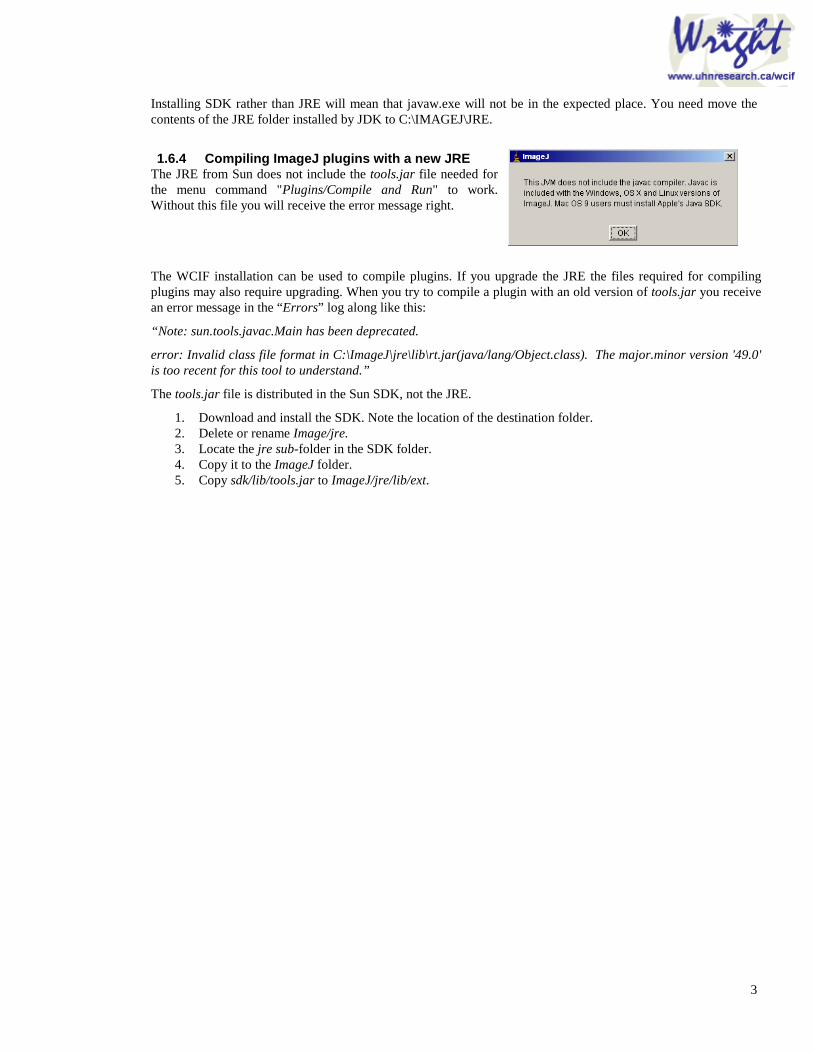
1.6.4 Compiling ImageJ plugins with a new JRE The JRE from Sun does not include the tools.jar file needed for the menu command "Plugins/Compile and Run" to work. Without this file you will receive the error message right.

The WCIF installation can be used to compile plugins. If you upgrade the JRE the files required for compiling plugins may also require upgrading. When you try to compile a plugin with an old version of tools.jar you receive an error message in the “Errors” log along like this:

“Note: sun.tools.javac.Main has been deprecated.

error: Invalid class file format in C:\ImageJ\jre\lib\rt.jar(java/lang/Object.class). The major.minor version '49.0' is too recent for this tool to understand.”

The tools.jar file is distributed in the Sun SDK, not the JRE.

1. Download and install the SDK. Note the location of the destination folder. 2. Delete or rename Image/jre. 3. Locate the jre sub-folder in the SDK folder. 4. Copy it to the ImageJ folder. 5. Copy sdk/lib/tools.jar to ImageJ/jre/lib/ext.

4

2 IMPORTING IMAGE FILES ImageJ primarily uses TIFF as the image file format. The menu command “File/Save” will save in TIFF format. The menu command “File/Open” will open TIFF files and import a number of other common file formats (e.g. JPEG, GIF, BMP, PGM, PNG). These natively supported files can also be opened by drag-and-dropping the file on to the ImageJ toolbar.

Several more file formats can be imported via ImageJ plugins (e.g. Biorad, Noran, Zeiss, Leica). When you subsequently save these files within ImageJ they will no longer be in their native format. Bear this in mind; ensure you do not overwrite original data.

There are further file formats such as PNG, PSD (Photoshop), ICO (Windows icon), PICT, which can be imported via the menu command “ File/Import/Jimi Reader…” .

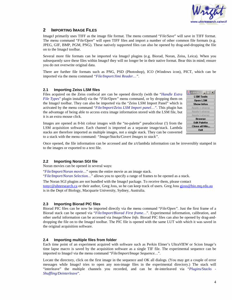
2.1 Importing Zeiss LSM files Files acquired on the Zeiss confocal are can be opened directly (with the “Handle Extra File Types” plugin installed) via the “File/Open” menu command, or by dropping them on the ImageJ toolbar. They can also be imported via the “Zeiss LSM Import Panel” which is activated by the menu command “File/Import/Zeiss LSM Import panel…”. This plugin has the advantage of being able to access extra image information stored with the LSM file, but it is an extra mouse click.

Images are opened as 8-bit colour images with the “no-palette” pseudocolour (!) from the LSM acquisition software. Each channel is imported as a separate image/stack. Lambda stacks are therefore imported as multiple images, not a single stack. They can be converted to a stack with the menu command: “Image/Stacks/Covert Images to stack”.

Once opened, the file information can be accessed and the z/t/lambda information can be irreversibly stamped in to the images or exported to a text file.

2.2 Importing Noran SGI file Noran movies can be opened in several ways:

“File/Import/Noran movie…” opens the entire movie as an image stack. “File/Import/Noran Selection…” allows you to specify a range of frames to be opened as a stack.

The Noran SGI plugins are not bundled with the ImageJ package. To receive them, please contact tonyc@uhnresearch.ca or their author, Greg Joss, so he can keep track of users. Greg Joss gjoss@bio.mq.edu.au is in the Dept of Biology, Macquarie University, Sydney, Australia.

2.3 Importing Biorad PIC files Biorad PIC files can be now be imported directly via the menu command “File/Open”. Just the first frame of a Biorad stack can be opened via “File/Import/Biorad First frame…”. Experimental information, calibration, and other useful information can be accessed via Image/Show Info. Biorad PIC files can also be opened by drag-and-dropping the file on to the ImageJ toolbar. The PIC file is opened with the same LUT with which it was saved in the original acquisition software.

2.4 Importing multiple files from folder Each time point of an experiment acquired with software such as Perkin Elmer’s UltraVIEW or Scion Image’s time lapse macro is saved by the acquisition software as a single TIF file. The experimental sequence can be imported to ImageJ via the menu command “File/Import/Image Sequence…”.

Locate the directory, click on the first image in the sequence and OK all dialogs. (You may get a couple of error messages while ImageJ tries to open any non-image files in the experimental directory.) The stack will “interleave” the multiple channels you recorded, and can be de-interleaved via “Plugins/Stacks - Shuffling/Deinterleave” .

5

Selected images that are not the same size can be imported as individual images windows using “File/Import/Selected files to open…” or as a stack with the “File/Import/Selected files for stack…”. Unlike the “File/Import/Image Sequence…” function, the images need not be of the same dimensions. If memory is limited, stacks can be opened as Virtual-Stacks with most of the stack remaining on the disk until it is required “File/Import/Disk based stack”.

2.5 Importing Multi-RAW sequence from folder To form an image, ImageJ needs to know the image dimensions, bit-depth, slice number per file and any extraneous information in the file format (offset and header size). All you really need to tell it is the image dimension in x and y. These values should be obtainable from the software in which the images were acquired. Armed with this information follow these steps:

1. File/Import/Raw…

2. Select experimental directory.

3. Typical values for the dialog box are: Image type = 16-bit unsigned (or 8 bit typically) width and height as determined earlier offset = 0, number of image = 1, gap = 0, ‘white’ is zero = off ‘Little-endian byte order’ = on, ‘open all files in folder’ = on to open all files in folder.

Non-image files will also be opened and may appear as blank images and need deleting: “Image/Stacks/Delete slice”. The stack will “interleave” the multiple channels you recorded, and can be de-interleaved via “Plugins/Stacks Shuffling/Deinterleave” .

2.6 Importing AVI and MOV files There are two plugins which can open uncompressed AVIs and some types of MOV file.

For opening (and writing) QuickTime you need a custom installation of QuickTime to include QT for Java (see section 1.3). QuickTime movies are then opened via “File/Import/QuickTime… ”.

Uncompressed AVIs can be opened via “File/Import/AVI…”.

2.7 Other Import functions Leica SP- Leica users, please contact me if you could supply a z- and t-series to test SP files with ImageJ.

Olympus Fluoview - available from http://rsb.info.nih.gov/ij/plugins/ucsd.html. Not bundled with the current download.

Animated GIF - This plugin opens an animated GIF file as an RGB stack. Also opens single GIF images.

IPLab…. Allows Windows IPLab files to be opened directly with the “File/Open” menu command, or drag-and-drop.

6

3 SAVING AND EXPORTING FILES The “File/Save” (hotkey: S) menu command will save the image as a TIF file. Other formats are available (see menu image on the right) and can be accessed by “File/Save As...”. When the “Save” or “Save as” dialog is opened, ImageJ will enter the image window’s name, plus the appropriate file suffix, as the “File Name”.

ImageJ will not add the suffix back if you delete it while changing the file name. This may make your file inaccessible from other programs, which require the suffix to identify the file format.

You can tell this from the name in the image window – it should display a suffix after it has been saved. If you have deleted the file suffix then resaving the file in the desired format usually restores it.

Animated GIF… This plugin saves a stack as an animated GIF. It works on RGB or 8 bit images.

PNG, PICT, XBM, TGA, Photoshop (PSD), XPM or PCX can be saved with “File/Save As/Jimi Writer…”. Run the plugin and select the desired format from the drop-down box.

Uncompressed AVI files are exported via either “File/Save as…/AVI…” and opened via “File/Save as/AVI..”. The frame-rate of the exported AVI movie is determined in the “Image/Stacks/Animation Options…” settings and can be between 0.1 and 100 frames per second (fps).

The AVI format that ImageJ saves is “uncompressed”. Uncompressed files are large, but should be playable on any PC/Mac without any decoder issues. There is freeware available that will convert between AVI types (e.g. RAD Video Tools) but once compressed, ImageJ will no longer be able to import them (unless you use the RAD video tools to resave them as uncompressed AVIs).

QuickTime MOV files are exported via the menu command “File/Save As/QuickTime Export” and opened via the menu command “File/Import/QuickTime…”.

The frame-rate of the final QuickTime movie is set in the dialog that pops up after you’ve named you *.MOV file. Compression settings are also set here. Despite this greater flexibility compared to AVI files, AVIs tend to be more MSWindows friendly and do not require a custom installation of QuickTime (see section 1.4).

Flash MX will import uncompressed AVI files. The frame-rate will then be determined by Flash, not the AVI movie file.

7

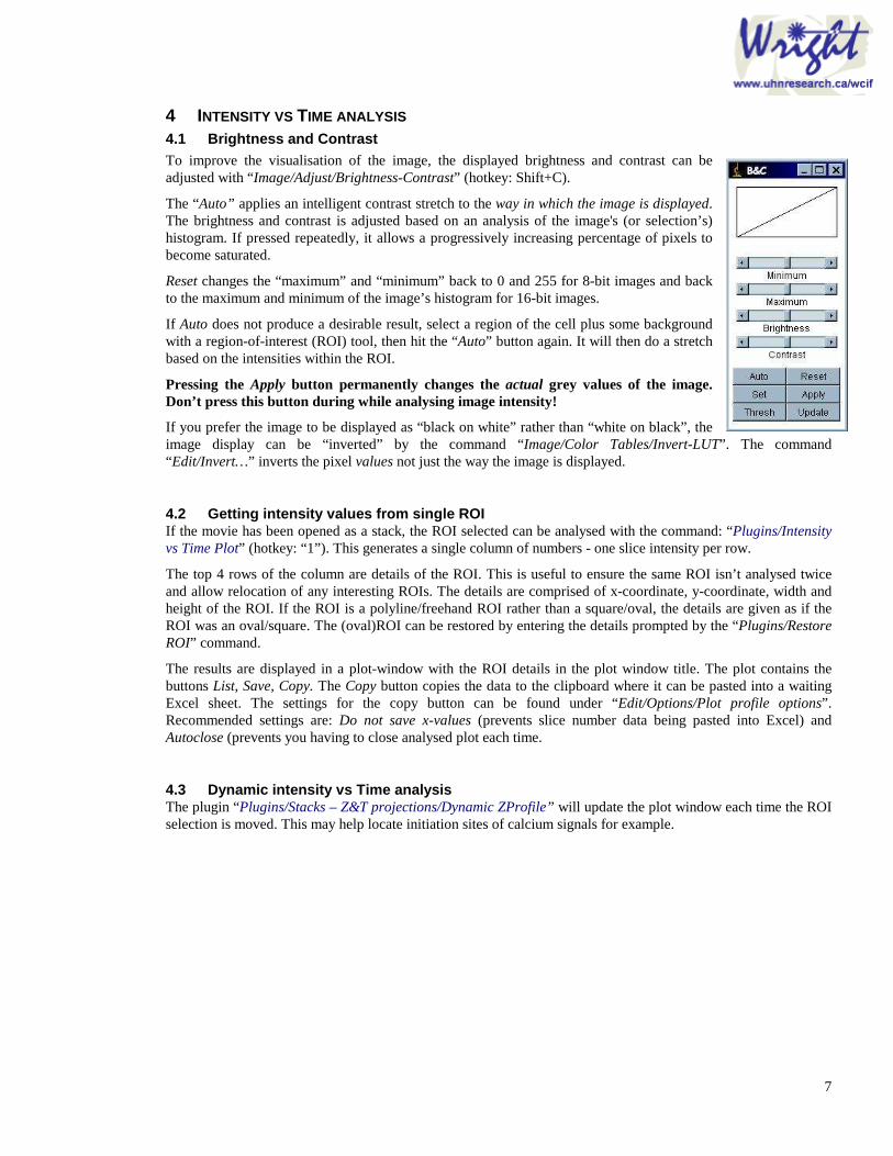
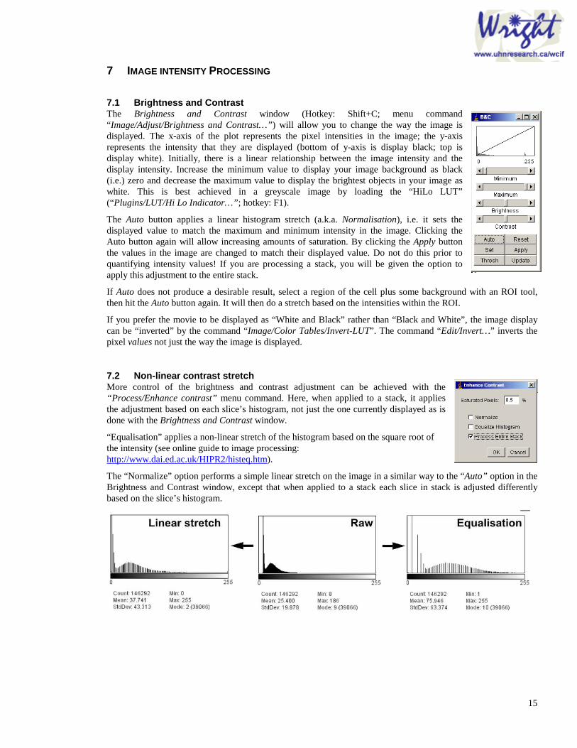
4 INTENSITY VS TIME ANALYSIS 4.1 Brightness and Contrast To improve the visualisation of the image, the displayed brightness and contrast can be adjusted with “Image/Adjust/Brightness-Contrast” (hotkey: Shift+C).

The “Auto” applies an intelligent contrast stretch to the way in which the image is displayed. The brightness and contrast is adjusted based on an analysis of the image's (or selection’s) histogram. If pressed repeatedly, it allows a progressively increasing percentage of pixels to become saturated.

Reset changes the “maximum” and “minimum” back to 0 and 255 for 8-bit images and back to the maximum and minimum of the image’s histogram for 16-bit images.

If Auto does not produce a desirable result, select a region of the cell plus some background with a region-of-interest (ROI) tool, then hit the “Auto” button again. It will then do a stretch based on the intensities within the ROI.

Pressing the Apply button permanently changes the actual grey values of the image. Don’t press this button during while analysing image intensity!

If you prefer the image to be displayed as “black on white” rather than “white on black”, the image display can be “inverted” by the command “Image/Color Tables/Invert-LUT”. The command “Edit/Invert…” inverts the pixel values not just the way the image is displayed.

4.2 Getting intensity values from single ROI If the movie has been opened as a stack, the ROI selected can be analysed with the command: “Plugins/Intensity vs Time Plot” (hotkey: “1”). This generates a single column of numbers - one slice intensity per row.

The top 4 rows of the column are details of the ROI. This is useful to ensure the same ROI isn’t analysed twice and allow relocation of any interesting ROIs. The details are comprised of x-coordinate, y-coordinate, width and height of the ROI. If the ROI is a polyline/freehand ROI rather than a square/oval, the details are given as if the ROI was an oval/square. The (oval)ROI can be restored by entering the details prompted by the “Plugins/Restore ROI” command.

The results are displayed in a plot-window with the ROI details in the plot window title. The plot contains the buttons List, Save, Copy. The Copy button copies the data to the clipboard where it can be pasted into a waiting Excel sheet. The settings for the copy button can be found under “Edit/Options/Plot profile options”. Recommended settings are: Do not save x-values (prevents slice number data being pasted into Excel) and Autoclose (prevents you having to close analysed plot each time.

4.3 Dynamic intensity vs Time analysis The plugin “Plugins/Stacks – Z&T projections/Dynamic ZProfile” will update the plot window each time the ROI selection is moved. This may help locate initiation sites of calcium signals for example.

8

4.4 Getting intensity values from multiple ROIs Multiple ROIs can be analysed at once using Bob Dougherty’s “Multi Measure” plugin. There is a native “ROI manager” function which does a similar job except the results generated are not sorted in to columns. Check Bob’s website for updates: http://www.optinav.com/ImageJplugins/list.htm

The Multi Measure plugin that comes with the installation is v2.

1. Open t-series.

2. It’s worthwhile generating a reference stack to add the ROIs to. Use the “ Image/Stacks/Z-project” function (hotkey: Shift+Z)♣. Select the “Average” option.

3. Rename this image “Ref expt name” or something memorable.

4. Open “Multi-measure” plugin (“Plugins/ROI/Multi Measure”).

5. Select background ROI first of all and to list with the Multi Measure dialog button “Add+Draw <CR>” (hotkey: Enter a.k.a. Carriage return). Continue adding cell ROIs.

6. Once finished selecting ROIs to be analysed in the reference image, save the reference image to the experiment’s data folder and then select the stack to be analysed.

7. Click Multi Measure dialog “Multi” (not the “Measure”) button to measure all the ROIs. Click “Yes” on “Process stack?” dialog.

8. Go to “Results” window. Select menu item “Edit/Select All…”. Then “Edit/Copy All”.

9. Go to Excel and paste data. With large data sets this can take some time so check you’re pasting new data in and not the last dataset copied from Multi Measure.

10. To copy ROI co-ordinates in to the Excel spreadsheet, ensure there is an empty row above the intensity data. Got to Multi Measure dialog and click “Copy list” button.

11. Go to Excel, select the empty cell above the first data column and then paste the ROI co-ordinates.

The ROIs can be stored and re-opened later using the Multi Measure dialog button “Save”. Save them in the experimental data folder. The ROIs can be opened later either individually (Multi Measure dialog button “Open”) or all at once (Multi Measure dialog button “Open All”) which opens all the ROIs in a folder.

Oval and rectangular ROIs can also be restored individually from x, y, l, h values using “Plugins/ROI/SpecifyROI…, , ” (hotkey: Shift + G).

♣ ImageJ assumes stacks to be z-series rather than t-series so many functions related to the third-dimension of an image stack are called “z-” something – e.g. “z-axis profile” is intensity over time plot.

9

4.5 Obtaining timestamp data

4.5.1 Zeiss LSM Once imported via the Zeiss LSM panel, the timestamp data can be extracted with the panel’s ‘Apply t-stamp’ button. This will then ask you if you want the timestamp to be added to the image, or displayed in a text file for saving/pasting to excel etc.

4.5.2 Noran In most instances the x-axis data, i.e. time of each frame, can be calculated from acquisition rates and frame number (e.g. frame 301 acquired with the acquisition rate set to 1 frame per 0.5 seconds was acquired at 25 minutes). However, the acquisition rate is non-linear, in the above experiment frame 301 was actually acquired at 25 minutes 12 seconds. Each frame has stored with it a “timestamp”, the precise time (in nanoseconds!) that it was acquired. This information can be extracted from an opened movie.

The movie must be opened as a stack and the timestamps can be extracted with the command: “Import/Noran timestamp (msec)” while the Noran Movie is open and selected. The timestamp data appears in the “Results” window. To copy data, click with the right mouse button on the windows, select “Select All”, then right-click again and select Copy. The timestamp data (accompanied by the movie filename) can then be pasted into Excel.

The Noran SGI plugins are not bundled with the ImageJ package. To receive them, please contact tonyc@uhnresearch.ca or their author, Greg Joss <gjoss@bio.mq.edu.au>, Dept of Biology, Macquarie University, Sydney, Australia.

4.5.3 Biorad This can be accessed via the menu command “Image/Show Info…”. Scroll down and it should give the time at which each slice was acquired. This can be selected, copied in to Excel and the time number obtained by searching and replacing (Excel menu command “Edit/Replace”) the text, leaving only the time data. The “elapsed” time can then be calculated by subtracting row 1 from all subsequent rows.

4.6 Pseudo-linescan “Linescanning” is a mode of acquisition common to many confocal microscopes where a single pixel wide line is acquired over a period of time instead of the norma1 2-D, x-y image. Usually this allows faster acquisition. The single pixel wide images over the time course are stacked from left to right to generate a 2-D image (i,e, x-t).

A “pseudo-linescan” is the generation of a linescan-type x-t plot from a 3-D (x, y, t) timecourse and can be useful in displaying 3-D data (x, y, t) in 2 dimensions.

A line of interest must be drawn followed by the command: “ Image/Stacks/Reslice” or keyboard “/”. It will prompt for the line width. Enter the width of line you wish to be averaged. A pseudo-linescan “stack” will be generated, each slice representing the pseudo-linescan of a single-pixel wide line along the line of interest. To average the pseudo-linescan “stack”, select “Image/Stacks/Z-Project…” and select the Average command. A polyline can be used although this will only allow a single pixel slice to be made.

This example shows the elementary calcium events preceding a calcium wave. HeLa cell loaded with the calcium-sensitive fluorophore, Fluo-3 and imaged whilst responding to application of histamine. A. Frame taken from time-course at the peak of the calcium-release response. (B) The line of pixels along X-Y was taken and stacked side by side from right-to left to generate a "pseudo-line scan". This allows visualisation of the progression of the wave from its initiation site.

10

5 PARTICLE ANALYSIS Particle counting can be done automatically if the specimen lends itself to it, i.e. the individual particles can touch – but not too much! If automatic particle counting cannot be done, ImageJ can facilitate manual counting with the “Point Picker” or “Cell counter” plugin.

5.1 Automatic Particle counting The biggest issue is one referred to as “segmentation” which is to distinguish the object from the background. Once the objects has been successfully segmented, they can then be analysed.

RAW Threshold Watershed “Analyze Particles” Merge

5.1.1 Threshold segmentation Automatic particle analysis requires the image to be a “binary” image i.e. black or white. The software needs to know exactly where the edges are to perform morphology measurements. A “threshold” range is set and pixels in the image whose value lies in this range are converted to black; pixels with values outside this range are converted to white (or vice-versa depending on what the user requests).

There are several ways to set thresholds. For monochrome images it is most simply done via thee menu command “ Image/Adjust/Threshold”. While the threshold is being set, the pixels within the threshold range are displayed in red. The user then changes then “Apply” the threshold and the image will be converted to a binary image.

For colour images, setting the threshold is a bit more complicated as each of the red, green and blue channels require different threshold ranges. The plugin “Plugins/Colour functions/Threshold Colour” can be used to do this most easily. This opens a fairly complicated and extensive control window. The simplest way to perfume a colour threshold is to use one of the selection tools to select one of the objects of interest, and then click the “Sample” button in the “Threshold Colour” control window. This should remove the pixels in the image that do not have pixels of the same colour as those in the selection. The thresholding can be manually tweaked with scroll bars in the histogram panes. It may be easier to conceptualise what you are doing at this point by switching the Control window from the default Hue, Saturation and Brightness colour model to red, green blue model by switching the option buttons at the bottom of the control window. The image can be displayed as a binary image with the “Threshold” button, and converted to a binary image via the menu command “Image/Type/8-bit” (?!).

11

5.1.2 Watershed segmentation Objects in a binary image that are slightly overlapping may be separated using the menu command “Process/Binary/Watershed”. This segmentation process is nicely illustrated with this figure from the ImageJ documentation web pages (http://rsb.info.nih.gov/ij/docs/index.html).

The image first needs to be converted to binary (set via thresholding). The black pixels are then replaced with grey pixels of an intensity proportional to their distance from a white pixel (i.e. black pixels close to the edge are light grey, those closer to the ‘middle) are nearer black. This is the Euclidian distance map (EDM). From this it calculated the centres of the objects the ultimate eroded points (UEPs), i.e. points that are equidistance from the edges. These points ere then dilated until the meet another black pixel, then a watershed line is drawn.

5.1.3 Analyse Particles Once the image has been segmented, the menu command “Analyze/Analyze particles” can be used to obtain various information regarding particle size and numbers.

Set the minimum size and maximum size to exclude objects that appear in the binary image that are clearly not objects of interest. Select the “Show: Outlines” option to display an image of the detected objects. This can then be merged with the original for presentation purposes. Invert the outline image and use the menu command “Plugins/Colour functions/Colour merge” to add the original and outline image.

The particle analysis can be automated via plugins or macros once the correct threshold value and particle size range has been determined for your objects of interest. See the “Plugins/Particle Analysis/ Nucleus counter” plugin and its source code to customise it to your images.

5.1.4 Particle tracking The “MTrack2” plugin (“Plugins/Particle counting/MTrack2”) tracks particles and reports their coordinates at each time-point and their total path length.

Raw Background corrected MultiTracker Motion paths Smoothed, Binary result of two objects

12

5.2 Manual Counting You can use the ImageJ toolbar Crosshair (mark and count) tool to count particles. However, a greater degree of control can be accessed with the “Point Picker” or “Cell counter” plugin.

5.2.1 Cell Counter When then “Plugins/Particle counting/Cell Counter” plugin) is run, a new Image window is generated with the original image plus four buttons along the bottom (Red type, Green type, Blue type and Yellow type). Clicking on a button changes the colour of the marking tool. The results table keeps a tally of the number of each of the cell types marked. Clicking the Results button will generate a summary of the data.

5.2.2 Point Picker “Plugins/Particle counting/PointPicker”. Running this plugin will change the ImageJ toolbar to the PointPicker toolbar (below).

Apply to single slice/all slices Return to ImageJ toolbar

Add Move Delete Import/Export Image Zoom Crosses Crosses Crosses point coordinates

Crosses are reversibly overlaid on to the image, incrementally changing colour (this differs from the Crosshair tool which irreversible stamps a point in the image). With the Point Picker tool, crosses can be moved and deleted. Once marking is complete, the cross coordinates can be accessed via the button.

This produces the “Point List” dialog allowing you to Show, Save or Open the points’ coordinates. Clicking “Show” displays the coordinates in the Results window, where they can be saved or copied to

the system clipboard. Once finished, you can return to the regular ImageJ toolbar by clicking the button.

13

6 COLOUR ANALYSIS

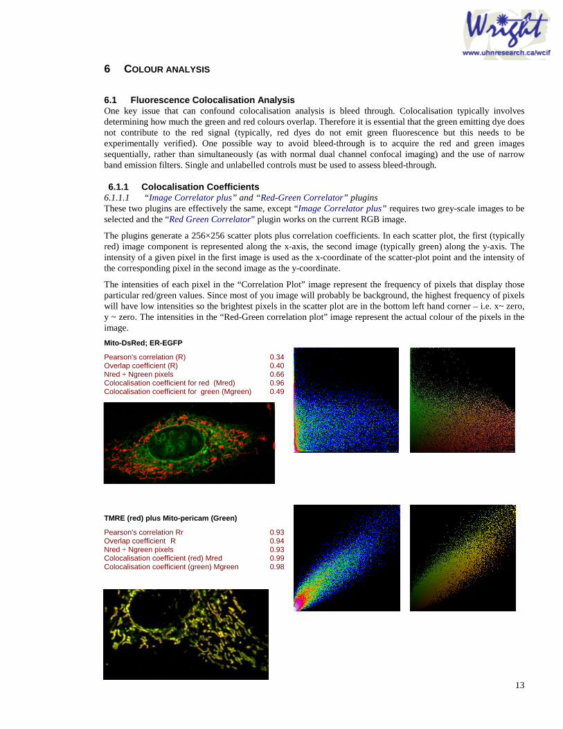
6.1 Fluorescence Colocalisation Analysis One key issue that can confound colocalisation analysis is bleed through. Colocalisation typically involves determining how much the green and red colours overlap. Therefore it is essential that the green emitting dye does not contribute to the red signal (typically, red dyes do not emit green fluorescence but this needs to be experimentally verified). One possible way to avoid bleed-through is to acquire the red and green images sequentially, rather than simultaneously (as with normal dual channel confocal imaging) and the use of narrow band emission filters. Single and unlabelled controls must be used to assess bleed-through.

6.1.1 Colocalisation Coefficients 6.1.1.1 “ Image Correlator plus” and “ Red-Green Correlator” plugins These two plugins are effectively the same, except “ Image Correlator plus” requires two grey-scale images to be selected and the “Red Green Correlator” plugin works on the current RGB image.

The plugins generate a 256×256 scatter plots plus correlation coefficients. In each scatter plot, the first (typically red) image component is represented along the x-axis, the second image (typically green) along the y-axis. The intensity of a given pixel in the first image is used as the x-coordinate of the scatter-plot point and the intensity of the corresponding pixel in the second image as the y-coordinate.

The intensities of each pixel in the “Correlation Plot” image represent the frequency of pixels that display those particular red/green values. Since most of you image will probably be background, the highest frequency of pixels will have low intensities so the brightest pixels in the scatter plot are in the bottom left hand corner – i.e. x~ zero, y ~ zero. The intensities in the “Red-Green correlation plot” image represent the actual colour of the pixels in the image.

Mito-DsRed; ER-EGFP

Pearson's correlation (R) 0.34 Overlap coefficient (R) 0.40 Nred ÷ Ngreen pixels 0.66 Colocalisation coefficient for red (Mred) 0.96 Colocalisation coefficient for green (Mgreen) 0.49

TMRE (red) plus Mito-pericam (Green)

Pearson's correlation Rr 0.93 Overlap coefficient R 0.94 Nred ÷ Ngreen pixels 0.93 Colocalisation coefficient (red) Mred 0.99 Colocalisation coefficient (green) Mgreen 0.98

14

The “Plugins/Stacks-RGB/Red-Green Correlator” plugin will take an RGB image, split it and then generate the correlation plots and data. It will work on the ROI in the original image or the whole image if no ROI is selected.

Both plugins generate various colocalisation coefficients: Pearson’s (Rr), Overlap (R) and Colocalisation (M1, M2) See Manders, E.E.M., Verbeek, F.J. & Aten, J.A. ‘Measurement of co-localisation of objects in dual-colour confocal images’, J. Microscopy, 169, 375-382, (1993). See tutorial sheet ‘Colocalisation’ for details.

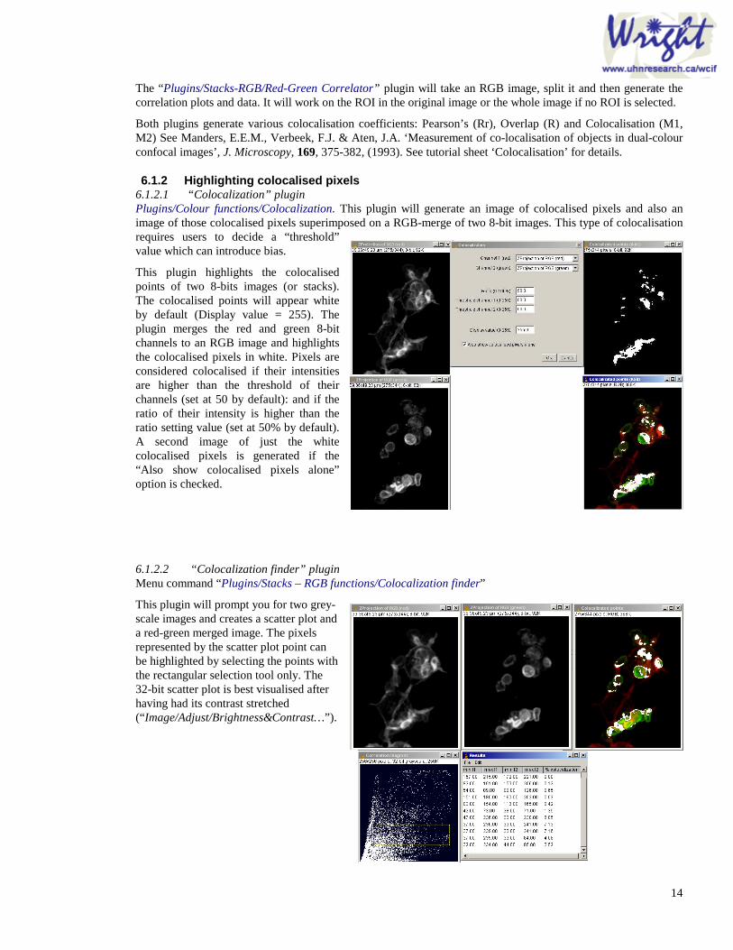
6.1.2 Highlighting colocalised pixels 6.1.2.1 “Colocalization” plugin Plugins/Colour functions/Colocalization. This plugin will generate an image of colocalised pixels and also an image of those colocalised pixels superimposed on a RGB-merge of two 8-bit images. This type of colocalisation requires users to decide a “threshold” value which can introduce bias.

This plugin highlights the colocalised points of two 8-bits images (or stacks). The colocalised points will appear white by default (Display value = 255). The plugin merges the red and green 8-bit channels to an RGB image and highlights the colocalised pixels in white. Pixels are considered colocalised if their intensities are higher than the threshold of their channels (set at 50 by default): and if the ratio of their intensity is higher than the ratio setting value (set at 50% by default). A second image of just the white colocalised pixels is generated if the “Also show colocalised pixels alone” option is checked.

6.1.2.2 “Colocalization finder” plugin Menu command “Plugins/Stacks – RGB functions/Colocalization finder”

This plugin will prompt you for two grey-scale images and creates a scatter plot and a red-green merged image. The pixels represented by the scatter plot point can be highlighted by selecting the points with the rectangular selection tool only. The 32-bit scatter plot is best visualised after having had its contrast stretched (“ Image/Adjust/Brightness&Contrast…”).

15

7 IMAGE INTENSITY PROCESSING

7.1 Brightness and Contrast The Brightness and Contrast window (Hotkey: Shift+C; menu command “ Image/Adjust/Brightness and Contrast…”) will allow you to change the way the image is displayed. The x-axis of the plot represents the pixel intensities in the image; the y-axis represents the intensity that they are displayed (bottom of y-axis is display black; top is display white). Initially, there is a linear relationship between the image intensity and the display intensity. Increase the minimum value to display your image background as black (i.e.) zero and decrease the maximum value to display the brightest objects in your image as white. This is best achieved in a greyscale image by loading the “HiLo LUT” (“Plugins/LUT/Hi Lo Indicator…”; hotkey: F1).

The Auto button applies a linear histogram stretch (a.k.a. Normalisation), i.e. it sets the displayed value to match the maximum and minimum intensity in the image. Clicking the Auto button again will allow increasing amounts of saturation. By clicking the Apply button the values in the image are changed to match their displayed value. Do not do this prior to quantifying intensity values! If you are processing a stack, you will be given the option to apply this adjustment to the entire stack.

If Auto does not produce a desirable result, select a region of the cell plus some background with an ROI tool, then hit the Auto button again. It will then do a stretch based on the intensities within the ROI.

If you prefer the movie to be displayed as “White and Black” rather than “Black and White”, the image display can be “inverted” by the command “Image/Color Tables/Invert-LUT”. The command “Edit/Invert…” inverts the pixel values not just the way the image is displayed.

7.2 Non-linear contrast stretch More control of the brightness and contrast adjustment can be achieved with the “Process/Enhance contrast” menu command. Here, when applied to a stack, it applies the adjustment based on each slice’s histogram, not just the one currently displayed as is done with the Brightness and Contrast window.

“Equalisation” applies a non-linear stretch of the histogram based on the square root of the intensity (see online guide to image processing: http://www.dai.ed.ac.uk/HIPR2/histeq.htm).

The “Normalize” option performs a simple linear stretch on the image in a similar way to the “Auto” option in the Brightness and Contrast window, except that when applied to a stack each slice in stack is adjusted differently based on the slice’s histogram.

16

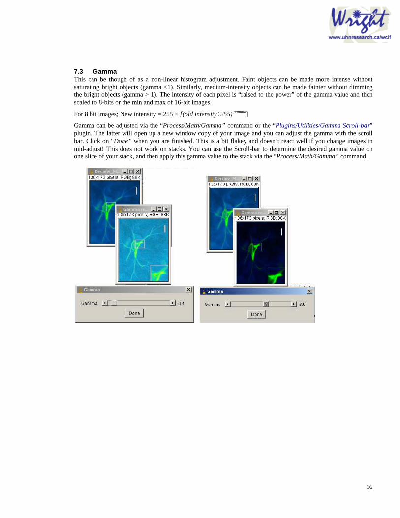
7.3 Gamma This can be though of as a non-linear histogram adjustment. Faint objects can be made more intense without saturating bright objects (gamma <1). Similarly, medium-intensity objects can be made fainter without dimming the bright objects (gamma > 1). The intensity of each pixel is “raised to the power” of the gamma value and then scaled to 8-bits or the min and max of 16-bit images.

For 8 bit images; New intensity = 255 × [(old intensity÷255) gamma]

Gamma can be adjusted via the “Process/Math/Gamma” command or the “Plugins/Utilities/Gamma Scroll-bar” plugin. The latter will open up a new window copy of your image and you can adjust the gamma with the scroll bar. Click on “Done” when you are finished. This is a bit flakey and doesn’t react well if you change images in mid-adjust! This does not work on stacks. You can use the Scroll-bar to determine the desired gamma value on one slice of your stack, and then apply this gamma value to the stack via the “Process/Math/Gamma” command.

17

7.4 Filtering See the online reference: http://www.dai.ed.ac.uk/HIPR2/filtops.htm for a simple explanation of digital filtering.

Filters can be found under the menu item “Process/Filters...” . Typically use a “Radius (pixels)” of 1 which equates to a 3×3 “kernel” – see online reference.

Mean filter: the pixel is replaced with the average of it and its neighbours within the radius. The menu item “Process/Smooth” is a 3×3 mean filter.

Gaussian filter: The is similar to smoothing but replaces the pixel with a pixel of value proportional to a normal distribution of it’s neighbours – not explained well, I know, but you’ve probably skipped the online reference and you need to read that to understand the way the filter works properly.

Median filter: the pixel is replaced with the median of it and its adjacent neighbours. This removes noise and preserves boundaries better than simple mean filtering, but can look odd. (The menu item “Process/Noise/Despeckle” is a 3×3 median filter).

Kalman filter: Sophisticated filtering for time-course experiments – a sort of “weighted running average”. Best used if the sample frequency is higher than the “event” frequency i.e. slowly occurring events. Otherwise you get odd, blurry results. “Process/Filter/Kalman Stack…”.

Sigma filter: A modification on the standard mean filter but preserves edges better – can be though of as a “gentle smooth”. The user specifies the kernel size, the Sigma width and the minimum number of pixels to include. A Sigma value for the kernel is calculated (based on the variance and mean of the intensities) and only pixels within this Sigma range (= Sigma × the user defined Sigma Width scaling factor) are used to calculate the mean. If there are too few pixels (exact number set in the user dialog: Minimum number of pixels) in the kernel that are within the Sigma range then the central pixel which is assumed to be spuriously low or high and the mean of the rest of the kernel is taken. Increasing the Sigma width and the minimum number of pixels results in increased smoothing and loss of edges. This plugin is under development, please send me any feedback..

J.S. Lee, Digital Image Smoothing and the Sigma Filter, Computer Vision, Graphics, and Image Processing 24, (1983) p. 255-269.

Raw Smooth Gaussian

Median Sigma Kalman

18

7.5 Background correction Background correction can be done in several ways and is facilitated if the grey image has the “Plugins/LUT/Hi Lo indicator” (Hotkey: F1) LUT loaded. This displays the zero values blue and the 255 white values red.

If the background is relatively even across the image, it is most simply remove with the Brightness&Contrast command – slowly raise the Minimum value until most of the background is displayed blue. The press the Apply button to change the grey-values and remove the background.

For uneven background the menu command “Process/Subtract background” can be used. This menu command removes uneven background from images using a “rolling ball” algorithm. The radius should be set to at least the size of the largest object that is not part of the background. It can also be used to remove background from gels where the background is white. Running the command several times may produce better results.

RAW “ Process/Subtract Background…”

Once the background has been evened, final adjustments can be made with the Brightness&Contrast control.

19

7.6 Flat-field correction

7.6.1 Proper correction This technique is applied to brightfield images. Uneven illumination, dirt/dust on lenses can result in a poor quality image. This can be corrected by acquiring a “flat-field” reference image with the same intensity illumination as the experiment. The flat field image should, ideally, be a field of view of the coverslip without any cells/debris. This is often not possible with the experimental coverslip, so a fresh coverslip may be used with approximately the same amount of buffer as the experiment. With fixed-specimens try removing the slide completely

1. Open both experimental image and flat-field image. 2. “Select all” of the flat-field image (hotkey: A) and measure the average intensity (hotkey: M). This value will

appear in the results window and represents your k1 value below. 3. Use the “Image Calculator plus” plugin (“Analyse/Tools/Calculator plus”). 4. i1 = experimental image; i2 = flat-field image; k1 = mean flat-field intensity; k2 = 0. This can also be done using the “Process/Image Calculator” function and ensuring the “32-bit Result” option is checked. You will then need to adjust the brightness and contrast and change the image to 8-bit.

7.6.2 Pseudo-correction Often it is not possible to obtain a flat-field reference image. However, it is still possible to correct for illumination intensity (although not small defects such as dust) by making a “pseudo-flat field” image by performing a large-kernel filter on the image to be corrected. This is particularly useful for DIC images where there is an intrinsic, and distracting, gradient in illumination.

The menu command “Process/Filters/Pseudo-flat field” automates this process. You are prompted to enter the kernel size for the mean filter; try the default value of 50 first. You can opt to keep the flat field image open to check whether the kernel is large enough. The object should not be visible in the flat field image.

RAW “Pseudo-flat field” Corrected

The first RAW image (top) pseudo-flat field corrected. Here the pseudo-flat field corrects for the uneven illumination but does not correct the dust specks. Compare this with the result of a proper flat-field correction above.

RAW Flat field Corrected

RAW Corrected

20

7.7 Masking unwanted regions 7.7.1 Simple masking

Draw around the area you want with one of the ROI tools then use: “Edit/Clear outside” . This will change area outside the selected region to the background value.

7.7.2 Complex masking A more sophisticated masking can be done by “thresholding” the image and subtracting this new binary image from the original.

1. Duplicate the image (if it’s a stack it’s worthwhile generating a “average projection” of a few frames).

2. Threshold this image using the menu command “Image/Adjust/Threshold” (hotkey Shift+T).

3. Hit the Auto button and then adjust the sliders until cells are all highlighted red.

4. Then click “Apply”. Check the tick box: “black foreground, white background”. You should now have a white and black image with your cells black and background white. If you have white cells and black background, invert the image with “Edit/Invert”.

5. This can be smoothed (“Process/Smooth”) and the black area enlarged slightly with “Process/Binary/Dilate” to give a better mask

6. Using the regular Image calculator “Process/Image calculator” subtract this black and white “mask” image from your original image/stack.

21

8 COLOUR IMAGE PROCESSING Images can have colour in two ways: pseudocolour or RGB. A pseudo-coloured image is a single channel, (i.e. grey) image that has colour ascribed to it via a “look up table” or LUT (a.k.a. palette, colour table). This is literally a table of grey values (zero to 256 or 4095 whether 8-bit or 12-bit grey) with accompanying red, green and blue values. So instead of displaying a grey, the image displays a pixel with a defined amount of each colour. Differences in colour in the pseudo-coloured image reflect differences in intensity of the object rather than differences in colour of the specimen that has been imaged. For pseudocolour functions see later.

The colours in RGB images (24-bit, 8-bits for each of the red, green and blue channels) and used to show multi-channel images. The colours are designed to reflect genuine colours, i.e. the green in an RGB image reflects green colour in the specimen, the differences in intensity of the green reflects differences in intensity of green in the specimen. There are several RGB functions in ImageJ. Native functions can be found in “Image/Color” and additional RGB functions can be found in “Plugins/Colour functions”.

Fluorescence and transmitted light brightfield images can be merged with the “Plugins/Colour functions/RGB-Grey Merge” plugin.

8.1 Merging multi-channel images Currently, only 24-bit colour images are supported, i.e. 8-bit red, green and blue channels. 48-bit colour image (i.e. 16-bit red, green and blue) processing is under development, but currently 16-bit grey images need to be converted to 8-bits before merging. This can be done by adjusting the Brightness&Contrast to the desired level and then using the menu command “Image/Type/8-bit”. Using the “Plugins/LUT/HiLo indicator” LUT can facilitate setting the brightness and contrast: zero is displayed as blue; saturated-white (255) as red.

The brightness and contrast of each channel is best adjusted prior to merging, however, each channel can be individually adjusted after merging with the “Image/Adjust/Color” function. This will not open the control panel if the “Brightness & contrast” control is already open.

8.1.1 Zeiss LSM multi-channel experiments Each channel in a Zeiss LSM file is imported as separate stacks. For single slice/time point, triple channel experiments this will produce 3 images – one for each of red, green and blue. Dual channel z- or t- series are imported as two separate stacks. To merge the red, green and blue components select Image/Color/RGB merge and put the appropriate image in the appropriate channel.

8.1.2 Biorad multi-channel experiments Dual channel, 3-D (i.e. xyz or xyt) experiments are saved as two separate files, one for each channel. Each file needs to be imported and then the stacks merged with the menu item: Image/Color/RGB merge. Typically, the red channel should be ***01.pic and the green ***02.pic.

Dual-channel, single frame experiments are saved as single PIC files with two slices. These can be RGB merged with ImageJ menu: “Image/Color/convert stack to RGB”. ImageJ assumes that if it’s a two slice stack, slice 1 is red and two is green and there is no blue channel.

Biorad dual-channel images acquired with CoMOS software have both channels displayed side by side in a single slice. The plugin “Plugins/Colour Functions/Biorad Aligner” will allow these images to be merged. The user can designate the colour for each half of the image from the drop-down option box. Brightness and crontrast of each half of the image can be adjusted separately by selecting each half of the image, adjusting and then applying the Brightness and Contrast change. To facilitate this, the keyboard function key “F4” selects the left hand image panel when pressed once, then the right hand image panel the next time it is pressed.

8.1.3 Interleaved multi-channel experiments Multi-channel experiments acquired on Noran and Perkin-Elmer systems are imported with the different channels interleaved, i.e. slice 1 is timepoint1-channel1, slice2 is timepoint1-channel2. The stack needs to be “De-interleaved” before it can be RGB-merged. This can be done with “Plugins/Stacks-Shuffling/DeInterleave” and entering the number of channels in the dialog (typically “2”). The two stacks can then be merged via: “ Image/Color/RGB merge”.

22

8.1.4 Colour merging An alternative to the normal Red-Green merge is to merge the images based on Cyan and Magenta, or Cyan-Yellow or any other colour combination.

This can aid visualisation of colocalisation due to our poor perception of red and green colours. The “Plugins/Colour functions/Colour Merge” function will perform a ‘difference’ arithmetic processing on the image stacks you select. This is not strictly a merge (when cyan and magenta merge they produce white, not yellow) but facilitates visualisation of the separate channels (See Demandolx and Davoust, J. Microscopy, 1997 v185. p21). You can perform a true merge if you turn off the “Difference” option.

Run the plugin and select the two images to be merged. Select the desired colours from the drop-down options. <Current> uses the LUT that the image currently has (this is often the desired LUT). The “Difference” option performs a “difference” arithmetic operation rather than a “addition”. If the “Pre-sub 2 from 1” option is checked the second image is subtracted from the first prior to merging. This may be useful for merging grey brightfield images with fluorescence where simple addition can result in washed-out look t the fluorescence image. It can look “unnatural” though. Another option may be to “darken” the brightfield image prior to merging (use menu command “Process/Math/Multiply” and use the value 0.5-0.75).

Normal merge Subtraction of red from grey prior to

merge Grey image multiplied by 0.75 prior to

normal merge

8.2 Pseudocolour Judicious use of LUTs can be very useful in highlighting the desired features of an image. The human eye can only perceive relatively few shades in one scene. Pseudo-colouring images can make the data more visible

Traditional “Green” LUT Enhanced “Green Hot” LUT Microtubules under nucleus now more apparent

23

Have a play and see which LUT helps illustrates the features in your image.

Montage compiled from a stack generated using the plugin “Plugins/LUT/List LUTs.

Different LUTs are available via the menu commands “ Image/Lookup table” and also “Plugins/LUT”. Custom LUTs can be made with the “Plugins/LUT/LUT panel”. Extra LUTs can be found in C:\ImageJ\LUT and can be applied by highlighting your image and selecting “Plugins/LUT/OpenLUT” then selecting the required *.lut file. Opening LUTs via this command rather than other ways (i.e. “File/Open…” or “File/Import/LUT…”) prevents the default folder from changing to “C:\ImageJ\LUT”. Custom LUTs can be made and edited using the “Plugins/LUT/LUT panel” plugin.

24

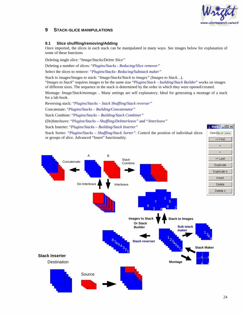
9 STACK-SLICE MANIPULATIONS

9.1 Slice shuffling/removing/Adding Once imported, the slices in each stack can be manipulated in many ways. See images below for explanation of some of these functions

Deleting single slice: “Image/Stacks/Delete Slice”

Deleting a number of slices: “Plugins/Stacks - Reducing/Slice remover”

Select the slices to remove: “Plugins/Stacks- Reducing/Substack maker”

Stack to images/Images to stack: “Image/Stacks/Stack to images” (Images to Stack…). “ Images to Stack” requires images to be the same size “Plugins/Stack – building/Stack Builder” works on images of different sizes. The sequence in the stack is determined by the order in which they were opened/created.

Montage: Image/Stack/montage… Many settings are self explanatory. Ideal for generating a montage of a stack for a lab book.

Reversing stack: “Plugins/Stacks – Stack Shuffling/Stack reverser”

Concatenate: “Plugins/Stacks – Building/Concatenator”

Stack Combine: “Plugins/Stacks – Building/Stack Combiner”

(De)Interleave: “Plugins/Stacks – Shuffling/DeInterleave” and “/Interleave”

Stack Inserter: “Plugins/Stacks – Building/Stack Inserter”

Stack Sorter: “Plugins/Stacks – Shuffling/Stack Sorter”. Control the position of individual slices or groups of slice. Advanced “Insert” functionality.

Destination

Stack Inserter

Source

AStackCombine

De-Interleave Interleave

Concatenate

B

24

123456

3

8

8

8

7

7

7

6

6

Montage

Sub-stackmaker

Stack to ImagesImages to Stack

Stack reverser5

5

4

43

321

1

1

8

Stack Maker

Montage

Or Stack Builder

25

9.2 Stack dimension manipulations Images and stacks can be resized and rotated with native functions or the more sophisticated TransformJ set of plugins from Erik Meijering. These are found in the “Plugins/TransformJ” menu list.

E. H. W. Meijering, W. J. Niessen, M. A. Viergever, Quantitative Evaluation of Convolution-Based Methods for Medical Image Interpolation, Medical Image Analysis, vol. 5, no. 2, June 2001, pp. 111-126.

More details can be found on this web-site: http://www.imagescience.org/meijering/software/transformj/

Spatial calibrations are lost so see the section on how to copy calibrations from one image to another with scaling (12.1.1.1)

26

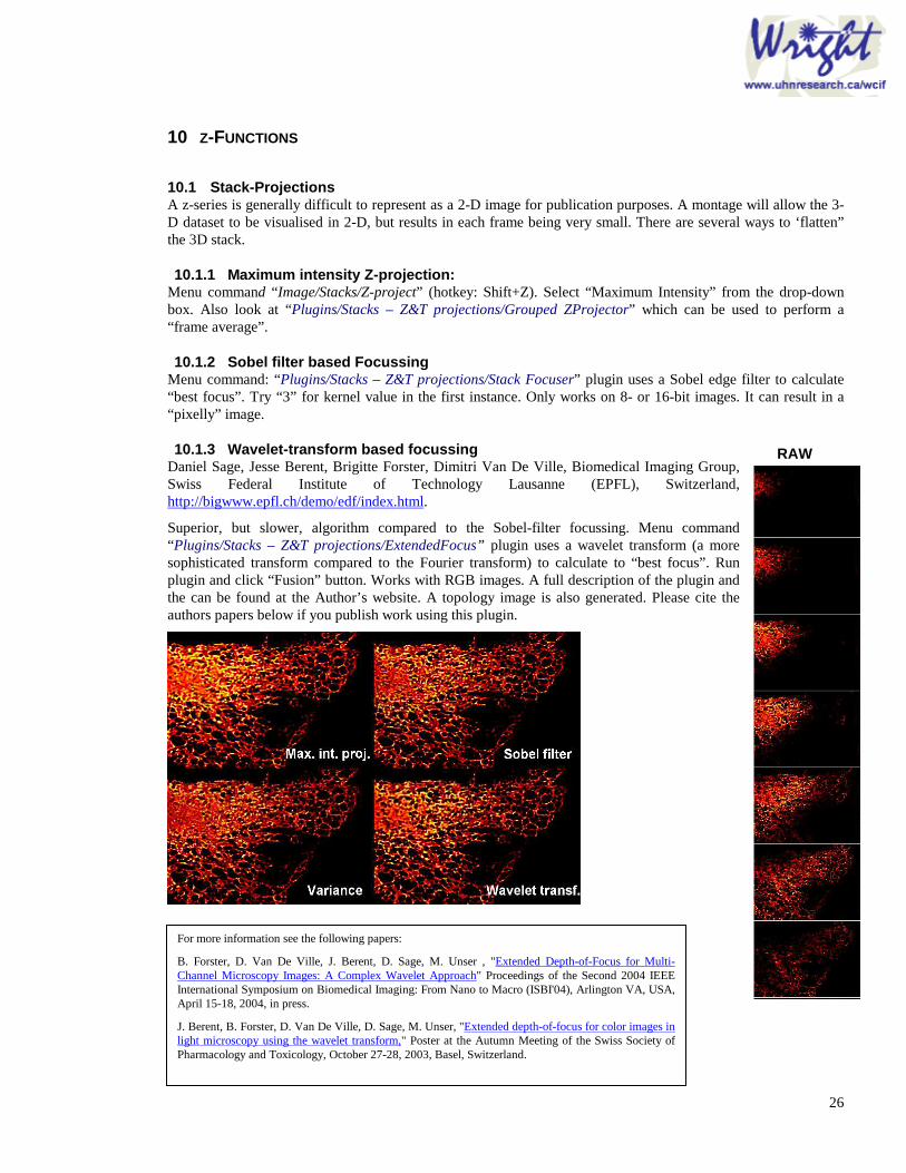
10 Z-FUNCTIONS

10.1 Stack-Projections A z-series is generally difficult to represent as a 2-D image for publication purposes. A montage will allow the 3-D dataset to be visualised in 2-D, but results in each frame being very small. There are several ways to ‘flatten” the 3D stack.

10.1.1 Maximum intensity Z-projection: Menu command “ Image/Stacks/Z-project” (hotkey: Shift+Z). Select “Maximum Intensity” from the drop-down box. Also look at “Plugins/Stacks – Z&T projections/Grouped ZProjector” which can be used to perform a “frame average”.

10.1.2 Sobel filter based Focussing Menu command: “Plugins/Stacks – Z&T projections/Stack Focuser” plugin uses a Sobel edge filter to calculate “best focus”. Try “3” for kernel value in the first instance. Only works on 8- or 16-bit images. It can result in a “pixelly” image.

10.1.3 Wavelet-transform based focussing Daniel Sage, Jesse Berent, Brigitte Forster, Dimitri Van De Ville, Biomedical Imaging Group, Swiss Federal Institute of Technology Lausanne (EPFL), Switzerland, http://bigwww.epfl.ch/demo/edf/index.html.

Superior, but slower, algorithm compared to the Sobel-filter focussing. Menu command “Plugins/Stacks – Z&T projections/ExtendedFocus” plugin uses a wavelet transform (a more sophisticated transform compared to the Fourier transform) to calculate to “best focus”. Run plugin and click “Fusion” button. Works with RGB images. A full description of the plugin and the can be found at the Author’s website. A topology image is also generated. Please cite the authors papers below if you publish work using this plugin.

Extended Focus

For more information see the following papers:

B. Forster, D. Van De Ville, J. Berent, D. Sage, M. Unser , "Extended Depth-of-Focus for Multi-Channel Microscopy Images: A Complex Wavelet Approach" Proceedings of the Second 2004 IEEE International Symposium on Biomedical Imaging: From Nano to Macro (ISBI'04), Arlington VA, USA, April 15-18, 2004, in press.

J. Berent, B. Forster, D. Van De Ville, D. Sage, M. Unser, "Extended depth-of-focus for color images in light microscopy using the wavelet transform," Poster at the Autumn Meeting of the Swiss Society of Pharmacology and Toxicology, October 27-28, 2003, Basel, Switzerland.

RAW

27

10.2 Volume render This is a 3D reconstruction method where the object will appear semitransparent.

Select the z-series stack then run the menu command: “Image/Stack/3D-Project”.

Try these initial settings:

1. Projection Method: Use “Brightest point” method.

2. Axis of Rotation: Select “y-axis”. There’s a bug which causes errors in x-axis rotation. If you want an x-axis rotation, prior to running the 3D-project command rotate the stack by 90° (Image/Rotate/Flip 90° right), 3D-project, the rotate the projection stack back 90° (Image/Rotate/Flip 90° left). Keep an eye out in the ImageJ/News web page to see if this bug is corrected.

3. Slice Spacing: This determines you aspect ratio of the stack. Biorad stacks are internally calibrated and this value should be correct – unless you set the wrong objective in the Biorad software during acquisition.

4. Interpolate when slice spacing > 0: check this option, although it will slow down the render so for a large data set it may be worthwhile having this “off” while you’re sorting out the settings.

10.3 Surface Render “Plugins/VolumeJ/VolumeJ”. This is a 3D reconstruction method where the object surface will appear opaque, giving a more “solid” look to the object. See: http://bij.isi.uu.nl/vj_manual.htm and http://bij.isi.uu.nl/vr.htm for updates.

Volume render

Please cite: M.D. Abràmoff, and M.A. Viergever. Computation and Visualization of Three Dimensional Motion in the Orbit. IEEE Trans Med Imag., 21 (4), 2002.

1. Select Volume stack that is to be rendered.

2. Select Classifier (i.e. render algorithm). Choose “Gradient no index” for greyscale stacks; chose “Ramp + index” for RGB stacks.

3. Set Classifier threshold as the intensity of the “surface” of the object. This can be determined using the “Image/Adjust/Threshold” command.

4. Set classifier deviation. High values result in blobby look, low values result in sharp edges. A good compromise is 1-2.

6. Set Rotation angle (try -20 first box to "tip” the volume backwards slightly).

7. Ensure Aspect ratio is correct – VolumeJ should pick up the spatial calibration of the stack if it is present.

8. Set Scale as 0.5 for faster preliminary renderings. Set it to 1 or 2 for final rendering.

9. Click on Render button to start rendering.

(10.) Click on Stop renderer if you’ve made a mistake!

Surface render

28

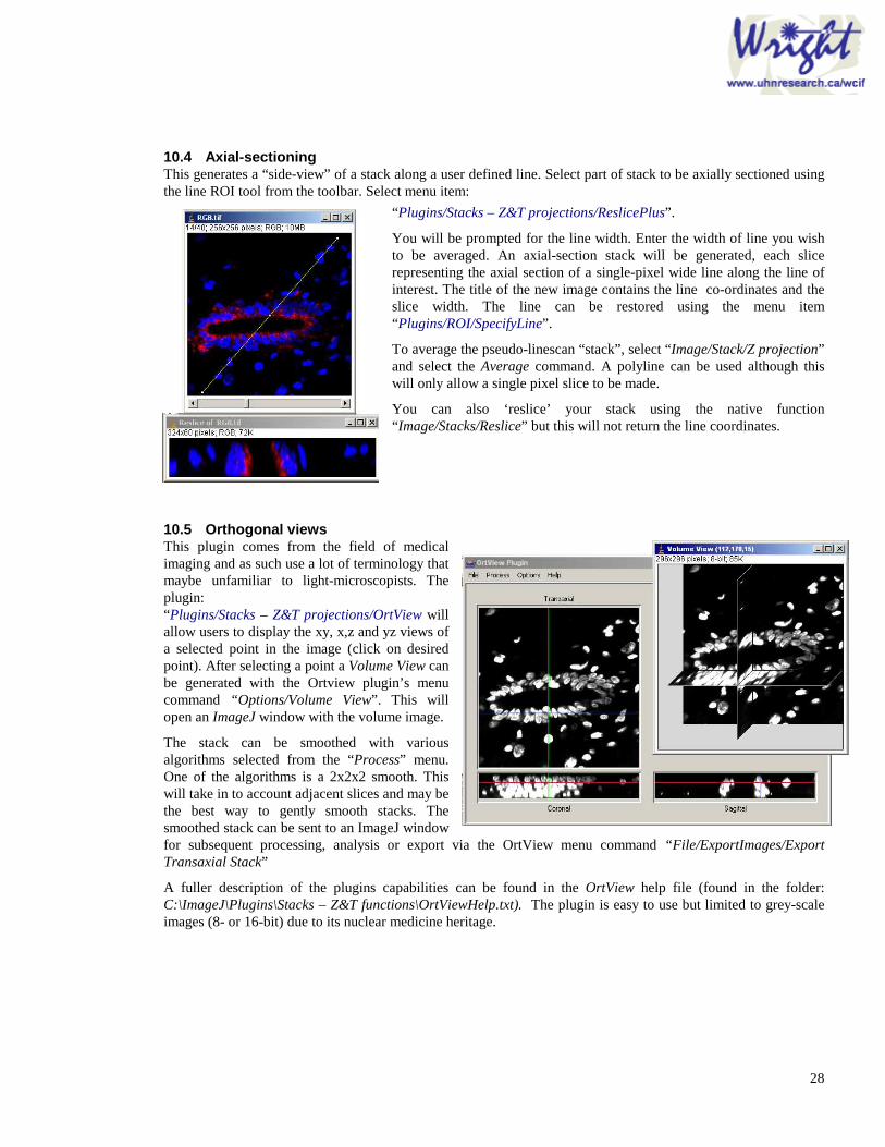
10.4 Axial-sectioning This generates a “side-view” of a stack along a user defined line. Select part of stack to be axially sectioned using the line ROI tool from the toolbar. Select menu item:

“Plugins/Stacks – Z&T projections/ReslicePlus”.

You will be prompted for the line width. Enter the width of line you wish to be averaged. An axial-section stack will be generated, each slice representing the axial section of a single-pixel wide line along the line of interest. The title of the new image contains the line co-ordinates and the slice width. The line can be restored using the menu item “Plugins/ROI/SpecifyLine”.

To average the pseudo-linescan “stack”, select “Image/Stack/Z projection” and select the Average command. A polyline can be used although this will only allow a single pixel slice to be made.

You can also ‘reslice’ your stack using the native function “ Image/Stacks/Reslice” but this will not return the line coordinates.

10.5 Orthogonal views This plugin comes from the field of medical imaging and as such use a lot of terminology that maybe unfamiliar to light-microscopists. The plugin: “Plugins/Stacks – Z&T projections/OrtView will allow users to display the xy, x,z and yz views of a selected point in the image (click on desired point). After selecting a point a Volume View can be generated with the Ortview plugin’s menu command “Options/Volume View”. This will open an ImageJ window with the volume image.

The stack can be smoothed with various algorithms selected from the “Process” menu. One of the algorithms is a 2x2x2 smooth. This will take in to account adjacent slices and may be the best way to gently smooth stacks. The smoothed stack can be sent to an ImageJ window for subsequent processing, analysis or export via the OrtView menu command “File/ExportImages/Export Transaxial Stack”

A fuller description of the plugins capabilities can be found in the OrtView help file (found in the folder: C:\ImageJ\Plugins\Stacks – Z&T functions\OrtViewHelp.txt). The plugin is easy to use but limited to grey-scale images (8- or 16-bit) due to its nuclear medicine heritage.

29

10.6 Stereo Pairs and Anaglyphs

10.6.1 Volume rendered-anaglyphs These plugins are under development and are at an early stage – please send feedback to tonyc@uhnresearch.ca.

This is an adaptation of the methods described at: http://rsb.info.nih.gov/nih-image/more-docs/confocals.html.

The menu command “Plugins/Stacks – Z&T projections/Stereo pair” plugin will create a side by side stereo pair from your stack and also a red-green anaglyph. The plugin will let you specify which of the stereo pair projections you want and also the angle of rotation between the pairs. Typical values would be 6-9°.

Stereo Pair

Red-Green Anaglyph Red-Cyan Anaglyph

30

10.6.2 Surface rendered-anaglyphs Surface stereo pairs are simply made with VolumeJ’s stereo pair button. This generates a stereo pair with a 5° difference.

These two images can be merged to form an anaglyph using either the menu command “Plugin/Colour Functions/Colour merge” or “ Image/Color/RGB merge”.

The “left eye” needs to be red; the “right eye” cyan or green.

Surface rendered anaglyph movies can be constructed using VolumeJ following an approach from Harvey Karten and Joel Sheffield.

1. Surface render your z-series (see Section 10.3 Surface Render) with a “Cine frame increment” of 6-9°.

2. Duplicate the Surface rendered movie.

3. Delete the top slice from the original movie.

4. Delete the last slice from the duplicate movie.

5. Merge the stacks using the menu command “Image/Color/RGB merge”.

6. Assign the duplicate stack as red and the original stack as green. For Red-Green anaglyphs set blue to be none; for red-cyan anaglyphs set the blue channel to be the same as the green.

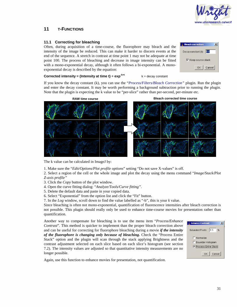
31

11 T-FUNCTIONS

11.1 Correcting for bleaching Often, during acquisition of a time-course, the fluorophore may bleach and the intensity of the image be reduced. This can make it harder to discern events at the end of the sequence. A stretch in contrast at time point 1 may not be adequate at time point 100. The process of bleaching and decrease in image intensity can be fitted with a mono-exponential decay, although it often follows a bi-exponential. A mono-exponential decay is described by the equation:

Corrected intensity = (Intensity at time t) ÷ exp -k×t k = decay constant

If you know the decay constant (k), you can use the “Process/Filters/Bleach Correction” plugin. Run the plugin and enter the decay constant. It may be worth performing a background subtraction prior to running the plugin. Note that the plugin is expecting the k value to be “per-slice” rather than per-second, per-minute etc.

The k value can be calculated in ImageJ by:

1. Make sure the “Edit/Options/Plot profile options” setting “Do not save X-values” is off. 2. Select a region of the cell or the whole image and plot the decay using the menu command “Image/Stack/Plot Z-axis profile” 3. Click the Copy button of the plot window. 4. Open the curve fitting dialog: “Analyze/Tools/Curve fitting”. 5. Delete the default data and paste in your copied data. 6. Select “Exponential” from the option list and click the “Fit” button. 7. In the Log window, scroll down to find the value labelled as “-b”, this is your k value. Since bleaching is often not mono-exponential, quantification of fluorescence intensities after bleach correction is not possible. This plugin should really only be used to enhance time-course movies for presentation rather than quantification.

Another way to compensate for bleaching is to use the menu item “Process/Enhance Contrast”. This method is quicker to implement than the proper bleach correction above and can be useful for correcting for fluorophore bleaching during a movie if the intensity of the fluorophore is changing only because of bleaching. Check the “Process Entire Stack” option and the plugin will scan through the stack applying Brightness and the contrast adjustment selected on each slice based on each slice’s histogram (see section 7.2). The intensity values are adjusted so that quantitative intensity measurements are no longer possible.

Again, use this function to enhance movies for presentation, not quantification.

RAW time course Bleach corrected time course

32

11.2 F÷F0

There are several drawbacks with the use of single wavelength fluorescent probes; some include uneven fluorescence intensity (F) due to cell thickness and cell to cell variation in loading. These can be largely corrected for by normalising fluorescence against resting fluorescence i.e. F0. This does not correct for bleaching and dye loss during the experiment.

First ensure the image is properly background corrected (7.5 Background correction).

1. Generate an “F0” image by averaging the first few frames of the stack. This can be done with the “ Image/Stacks/Z-project” ♣ menu item, using the “Average” drop-down box option. Select “Start slice” as 1 and “Stop Slice” as 5-10 depending on how many frames you wish to average. Rename the new z-projected image (“Image/Rename”) “Fzero”.

2. Open the “Image Calculator Plus” via “Process/Image Calculator”.

3. Image 1 = Original stack

4. Image 2 = image “Fzero”

5. Operation = “Divide”

6. Select “32-bit Result” and “Create New Window”

7. Rename this result window (“Image/Rename”) FdivF0.

8. The maximum and minimum intensity in the stack can be determined with the “Analyze/Tools/Stack Histogram” plugin.

9. Using the Brightness and Contrast (See section 4.1) dialog set the maximum and minimum to these values.

10. Convert the 32-bit stack to 8-bit (“Image/Type/8-bit”).

11. The Images in FdivF0 will probably have a noisy background between the cells and need to be cleaned up. Using your original stack, create a mask of the cells. This is done by first thresholding the original; stack (“ Image/Adjust/Threshold”). Hit the Auto button and then adjust the sliders until cells are all highlighted red. Then click “Apply”. Check the tick box: “black foreground, white background”. You should now have a white and black image with your cells black and background white. If you have white cells and black background, invert the image with “Edit/Invert”.

12. Using the Image calculator “Process/Image calculator” to subtract this black and white stack from your FdivF0 stack.

13. Pseudocolour to taste.

This process could relatively easily be automated via a plugin or macro. However, due to multiple user-defined steps (i.e. how many frames for the Z-projection, the thresholding of the original stack for the mask, whether it’s better to correct for bleaching before thresholding the stack) I have not done so.

♣ ImageJ assumes stacks to be z-series rather than t-series so many functions related to the third-dimension of an image stack are called “z-” something – e.g. “z-axis profile” is an “intensity vs time” plot.

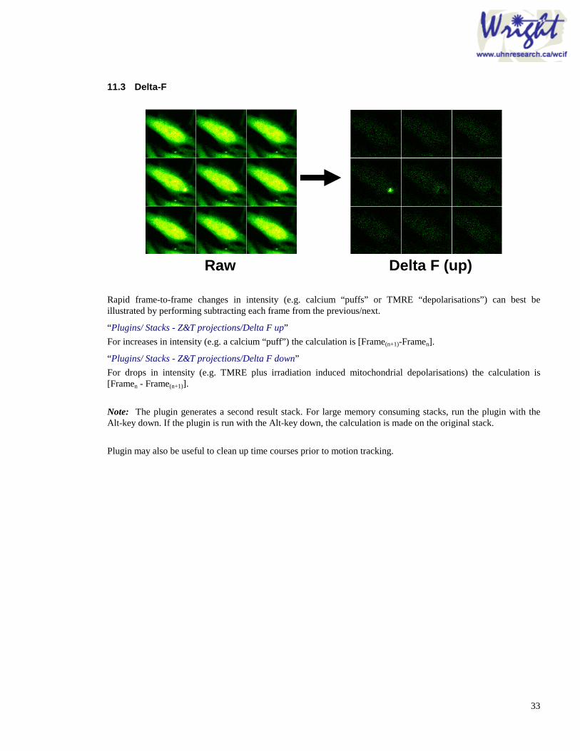
33

11.3 Delta-F

Rapid frame-to-frame changes in intensity (e.g. calcium “puffs” or TMRE “depolarisations”) can best be illustrated by performing subtracting each frame from the previous/next.

“Plugins/ Stacks - Z&T projections/Delta F up”

For increases in intensity (e.g. a calcium “puff”) the calculation is [Frame(n+1)-Framen].

“Plugins/ Stacks - Z&T projections/Delta F down”

For drops in intensity (e.g. TMRE plus irradiation induced mitochondrial depolarisations) the calculation is [Framen - Frame(n+1)].

Note: The plugin generates a second result stack. For large memory consuming stacks, run the plugin with the Alt-key down. If the plugin is run with the Alt-key down, the calculation is made on the original stack.

Plugin may also be useful to clean up time courses prior to motion tracking.

Raw Delta F (up)

34

11.4 Surface plotting

Surface plots can be generated in two ways: via the menu command “Analyze/Surface plot” or via the plugin “Plugins/VolumeJ/SurfaceJ”. These functions will surface-plot movies as well as single frame images. Ensure the features you’re interested in are “Contrast stretched” optimally. This can be done using a “Max intensity projection” on the stack. Getting the max and min pixel intensities and applying these to the stack. Remember, do not perform intensity analysis on images that have had their contrast stretched.

11.4.1 “Analyze/Surface plot ” settings When this function is selected, a dialog will appear. Try the settings below first and play with them to optimise the surface plot. The LUT of the final surface plot is taken from the LUT of the image.

11.4.2 SurfaceJ settings You can surface plot either a single frame or a movie. Surface rendering is a slow process so it is best to pick a frame from the movie that shows the features you’re trying to demonstrate. Duplicate this (Ctrl+D) and use it as a test image to get the best settings for surface plotting your movie.

Select the image to be rendered with the “Source image(s)” drop down box.

The options with three text-entry boxes along side represent x, y and z values.

“Rotate(°):” value of -20 in the first (x-axis) box gives a good 3D effect. Play with this.

“Scale”. Set to 0.5 speeds things along also when adjusting the settings and set to 2 or more for the final surface plotting.

“Aspect /:” Surface plot is can be stretched in “height” by increasing the z-axis aspect (i.e. the third) box. Although 1 is usually OK if you’ve stretched the contrast properly. This will not affect the pseudocolour of the peaks which is determined by the pixel intensity.

“ Index LUT”: by default the plot will have the “spectrum” LUT. Change this drop-down box to “Load custom” and you’ll be prompted to locate a desired LUT when you start the surface-plot

“Gaussian Smoothing” value of 2-4. This slows rendering down but gives smoother surface plot.

“Rendering surface plot”: starts surface plotting.

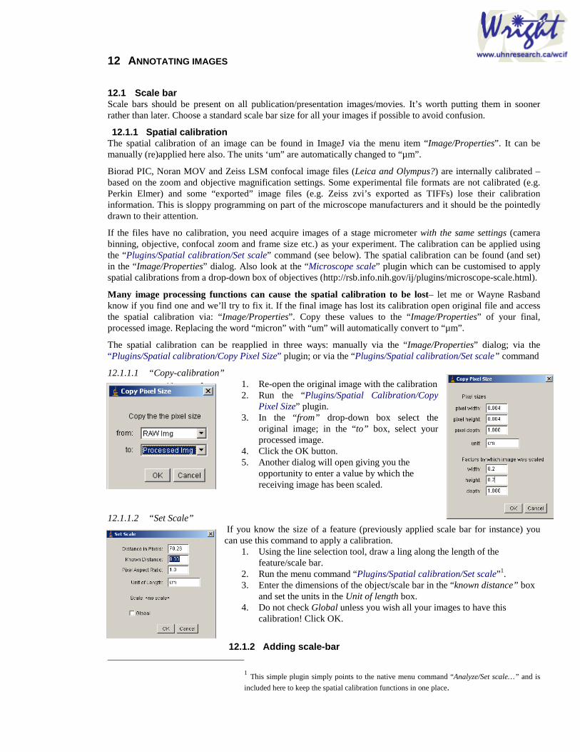
12 ANNOTATING IMAGES

12.1 Scale bar Scale bars should be present on all publication/presentation images/movies. It’s worth putting them in sooner rather than later. Choose a standard scale bar size for all your images if possible to avoid confusion.

12.1.1 Spatial calibration The spatial calibration of an image can be found in ImageJ via the menu item “Image/Properties”. It can be manually (re)applied here also. The units ‘um” are automatically changed to “µm”.

Biorad PIC, Noran MOV and Zeiss LSM confocal image files (Leica and Olympus?) are internally calibrated – based on the zoom and objective magnification settings. Some experimental file formats are not calibrated (e.g. Perkin Elmer) and some “exported” image files (e.g. Zeiss zvi’s exported as TIFFs) lose their calibration information. This is sloppy programming on part of the microscope manufacturers and it should be the pointedly drawn to their attention.

If the files have no calibration, you need acquire images of a stage micrometer with the same settings (camera binning, objective, confocal zoom and frame size etc.) as your experiment. The calibration can be applied using the “Plugins/Spatial calibration/Set scale” command (see below). The spatial calibration can be found (and set) in the “Image/Properties” dialog. Also look at the “Microscope scale” plugin which can be customised to apply spatial calibrations from a drop-down box of objectives (http://rsb.info.nih.gov/ij/plugins/microscope-scale.html).

Many image processing functions can cause the spatial calibration to be lost– let me or Wayne Rasband know if you find one and we’ll try to fix it. If the final image has lost its calibration open original file and access the spatial calibration via: “Image/Properties”. Copy these values to the “Image/Properties” of your final, processed image. Replacing the word “micron” with “um” will automatically convert to “µm”.

The spatial calibration can be reapplied in three ways: manually via the “Image/Properties” dialog; via the “Plugins/Spatial calibration/Copy Pixel Size” plugin; or via the “Plugins/Spatial calibration/Set scale” command

12.1.1.1 “Copy-calibration” 1. Re-open the original image with the calibration 2. Run the “Plugins/Spatial Calibration/Copy

Pixel Size” plugin. 3. In the “from” drop-down box select the

original image; in the “to” box, select your processed image.

4. Click the OK button. 5. Another dialog will open giving you the

opportunity to enter a value by which the receiving image has been scaled.

12.1.1.2 “Set Scale”

If you know the size of a feature (previously applied scale bar for instance) you can use this command to apply a calibration.

1. Using the line selection tool, draw a ling along the length of the feature/scale bar.

2. Run the menu command “Plugins/Spatial calibration/Set scale” 1. 3. Enter the dimensions of the object/scale bar in the “known distance” box

and set the units in the Unit of length box. 4. Do not check Global unless you wish all your images to have this

calibration! Click OK.

12.1.2 Adding scale-bar

1 This simple plugin simply points to the native menu command “Analyze/Set scale…” and is

included here to keep the spatial calibration functions in one place.

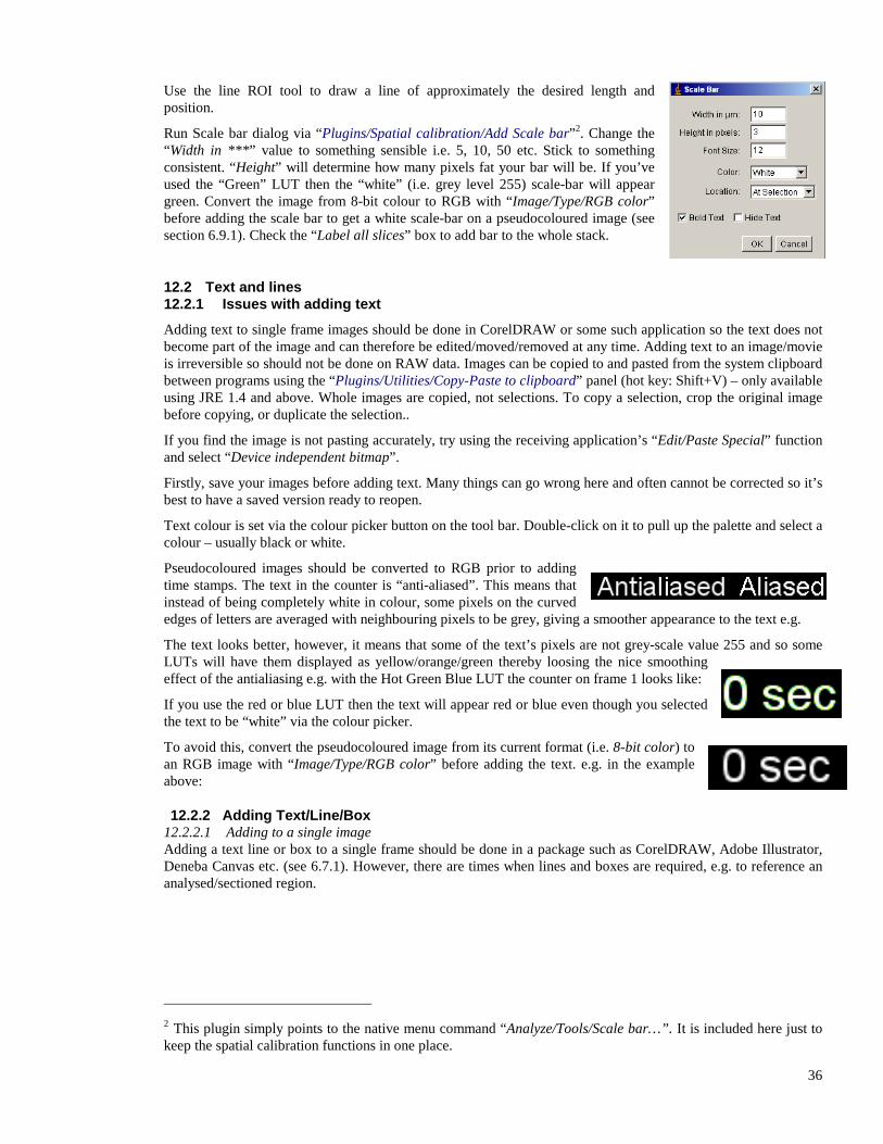
36

Use the line ROI tool to draw a line of approximately the desired length and position.

Run Scale bar dialog via “Plugins/Spatial calibration/Add Scale bar” 2. Change the “Width in *** ” value to something sensible i.e. 5, 10, 50 etc. Stick to something consistent. “Height” will determine how many pixels fat your bar will be. If you’ve used the “Green” LUT then the “white” (i.e. grey level 255) scale-bar will appear green. Convert the image from 8-bit colour to RGB with “Image/Type/RGB color” before adding the scale bar to get a white scale-bar on a pseudocoloured image (see section 6.9.1). Check the “Label all slices” box to add bar to the whole stack.

12.2 Text and lines 12.2.1 Issues with adding text

Adding text to single frame images should be done in CorelDRAW or some such application so the text does not become part of the image and can therefore be edited/moved/removed at any time. Adding text to an image/movie is irreversible so should not be done on RAW data. Images can be copied to and pasted from the system clipboard between programs using the “Plugins/Utilities/Copy-Paste to clipboard” panel (hot key: Shift+V) – only available using JRE 1.4 and above. Whole images are copied, not selections. To copy a selection, crop the original image before copying, or duplicate the selection..

If you find the image is not pasting accurately, try using the receiving application’s “Edit/Paste Special” function and select “Device independent bitmap”.

Firstly, save your images before adding text. Many things can go wrong here and often cannot be corrected so it’s best to have a saved version ready to reopen.

Text colour is set via the colour picker button on the tool bar. Double-click on it to pull up the palette and select a colour – usually black or white.

Pseudocoloured images should be converted to RGB prior to adding time stamps. The text in the counter is “anti-aliased”. This means that instead of being completely white in colour, some pixels on the curved edges of letters are averaged with neighbouring pixels to be grey, giving a smoother appearance to the text e.g.

The text looks better, however, it means that some of the text’s pixels are not grey-scale value 255 and so some LUTs will have them displayed as yellow/orange/green thereby loosing the nice smoothing effect of the antialiasing e.g. with the Hot Green Blue LUT the counter on frame 1 looks like:

If you use the red or blue LUT then the text will appear red or blue even though you selected the text to be “white” via the colour picker.

To avoid this, convert the pseudocoloured image from its current format (i.e. 8-bit color) to an RGB image with “Image/Type/RGB color” before adding the text. e.g. in the example above:

12.2.2 Adding Text/Line/Box 12.2.2.1 Adding to a single image Adding a text line or box to a single frame should be done in a package such as CorelDRAW, Adobe Illustrator, Deneba Canvas etc. (see 6.7.1). However, there are times when lines and boxes are required, e.g. to reference an analysed/sectioned region.

2 This plugin simply points to the native menu command “Analyze/Tools/Scale bar…”. It is included here just to keep the spatial calibration functions in one place.

37

Drawing of lines/boxes is achieved by first selecting the desired line/box in the image with the line/Rectangle ROI tool from the toolbar or defining the line/box via “Plugins/Specify ROI…” or “Plugins/Specify Line…”. The line/box can be resized here to the desired size/shape with the small square handles on the ROI. The line/box can then be stamped in to the image by right clicking on the image and selecting “Draw”. This will add the box/line to a single frame, the colour determined by the by the color picker toolbar button and the width in pixels defined in “Edit/Options/Line width”. Adding text is done by the toolbar’s text button. Click the toolbar; click the image; write the desired text. The font size is set by double clicking the toolbar-text button, the colour determined by the by the color picker toolbar button. Antialiasing can be turned on/off via the menu item “Edit/Options/Miscellaneous” (although this option does not affect the `Stamper plugins which have antialiasing on permanently). The text is stamped in to the image by right clicking and selecting “Draw”.

12.2.2.2 Adding to movie-stack Drawing/writing on a stack only adds the drawn object to the current slice*. If you want the text/box/line to be added to an entire “movie stack” you need to create a new single frame image add the text/box/line to this and then add this single frame to the “movie stack”. This is best done by:

1. Duplicate a frame from the “movie stack” (“Image/Duplicate” and disable “Duplicate entire stack” option).

2. Rename (“Image/Rename”) “text/box/line image”

3. Select the whole image (“Edit/Selection/Select all” or Shift-A)

4. Edit/Clear

5. Go to the “movie stack” and select the desired text/box/line (see 6.7.2.1 above).

6. Go to the “text/box/line image”

7. Restore the selection by “Edit/Selection/Restore” – or Shift-E.

8. Draw the selection (right click the selection and select Draw)

9. Use the Image Calculator (“Image/Calculator”) to add the “text/box/line image” to the “movie image”.

*This may become redundant as ImageJ develops. Keep a look out in the ImageJ/News web page.

12.2.3 Adding timestamps 1. Draw a rectangular ROI at the location and of the approximate size of the desired counter. The text will, by

default be of the same height as the ROI and aligned to its left edge. Ensure it is not too close to the edge of the image. This will result in a bar underneath the counter e.g.

2. Run the “Plugins/Movies/Time Stamper” .

3. Enter appropriate settings. The X and Y location and font size are taken from the ROI and can be changed at this point.

Remember, the bigger the text, the smoother it will look and the easier the timestamp will be to read. Bigger is better. It may be worth changing it to a consistent value for all your movies.

Also, bear in mind that the interval needn’t be “time". The Time Stamper plugin also can be used to add “z-axis depths” to z-stacks and “angle of rotation” to rotating volume movies ( ° = Alt+247; µ = Alt+230).

12.2.4 Adding event marker to movie The “Plugins/Movies/Event Stamper” plugin can be used to add text to a movie for a designated number of frames, e.g. “Agonist ON”. This is simply done by running the Event Stamper plugin setting the desired text in the “Text” box, enter start frame and end frame and click OK. The text size and location is taken from the current ROI and can be changed once the dialog is opened.

38

13 APPENDIX 1: PLUGIN AUTHORS

Animated GIF Kevin Weiner, FM Software, W. Rasband., 5

Animated Gif… Ryan Raz (http://rraz.ca)

AVI… Daniel Marsh (marshd@ninds.nih.gov), 5

Calculator plus Wayne Rasdband, 19

Cell Counter Kurt De Vos (kd269@columbia.edu), 12

Colocalization Pierre Bourdoncle (bourdoncle@ijm.jussieu.fr), Institut Jacques Monod, Service Imagerie, Paris, 14

Colocalization finder Christophe Laummonerie, Jerome Mutterer, Institut de Biologie Moleculaire des Plantes, Strasbourg, France., 14

Concatenator Wayne Rasband, 24

Copy Pixel Size J. Anthony Parker, MD PhD (J.A.Parker@IEEE.org), 35

Copy-Paste to clipboard Amrit Aneja and Wayne Rasband, 36

Cyan Magenta Merge Tony Collins, Wayne Rasband, 22

Deinterleave Russell Kincaid (rekincai@syr.edu), Tony Collins, 4

DeInterleave Tony Collins, Russel Kincaid, 24

Delta F down Tony Collins, 33

Delta F up Tony Collins, 33

Disk based stack Wayne Rasband, 5

Dynamic ZProfile Kevin (Gali) Baler (gliblr at yahoo.com) and Wayne Rasband, 7

ExtendedFocus Jesse Berent, Brigitte Forster, Dimitri Van De Ville, Daniel Sage & Michael Unser, 26

Grouped ZProjector Charlie Holly, caholly at colby.edu, 26

Handle Extra File Types Gregory Jefferis (jefferis at Stanford.edu), 4

Image Correlator plus Wayne Rasband, Tony Collins, 13

Interleave J. Anthony Parker, MD PhD (J.A.Parker@IEEE.org), 24

IPLab reader Wayne Rasband (wsr at nih.gov), 5

Jimi Reader… Wayne Rasband and Ulf Dittmer (udittmer at mac.com), 4

Jimi Writer… Jeffrey Kuhn (jkuhn@ccwf.cc.utexas.edu) The University of Texas at Austin, 6

Kalman filter Christopher Philip Mauer (cpmauer@northwestern.edu), 17

Leica SP Nico Stuurman (Stuurman@rulbim.leidenuniv.nl) and Wayne Rasband, 5

List LUTs G. Landini. http://www.dentistry.bham.ac.uk/landinig/software/software.html

LUT panel Patrick Pirrotte & Jerome Mutterer (jerome.mutterer at ibmp-ulp.u-strasbg.fr, http://www-ibmp.u-strasbg.fr/sg/microscopie/methods/lut/lut.htm )

Microscope scale Paul Baggethun (Paul.Baggethun@ALCOA.COM), 35

MTrack2 Nico Stuurman (nicos@itsa.ucsf.edu), 11

Multi Measure Wayne Rasband, Bob Dougherty, 8

Noran movie… Greg Joss (gjoss@bio.mq.edu.au), 4

Noran Selection… Greg Joss (gjoss@bio.mq.edu.au), 4

Noran timestamp (msec) Greg Joss <gjoss@bio.mq.edu.au>, 9

OpenLUT, 23

OrtView Paulo Bonetto (bonetto@disi.unige.it), 28

PointPicker Philippe Thévenaz (philippe.thevenaz@epfl.ch), 12

39

Process/Filters/Bleach Correction Tony Collins, Wayne Rasband, 31

Process/Filters/Pseudo-flat field Tony Collins, 19

QuickTime Export Wayne Rasband, 6

QuickTime… Wayne Rasband (wsr at nih.gov), Robert Dougherty (www.optinav.com) Jeff Hardin (jdhardin at facstaff.wisc.edu), 5 Wayne Rasband (wsr at nih.gov), Robert Dougherty (www.optinav.com), Jeff Hardin (jdhardin at facstaff.wisc.edu), 6

Red Green Correlator Wayne Rasband, Tony Collins, 13

Red-Green Correlator Wayne Rasband, Tony Collins, 14

ReslicePlus Tony Collins, Wayne Rasband, 28

RGB Grey Merge Eugene Tkachenko (etkachen@Dartmouth.EDU) & Justin D. Pearlman, 21

Selected files for stack… Albert Cardona albert@pensament.REMOVE-MEnet, 5

Selected files to open… Wayne Rasband, 5

Slice remover Wayne Rasband, 24

Specify Line… Wayne Rasband, 36

Specify ROI… Jeffrey Kuhn (jkuhn@ccwf.cc.utexas.edu), The University of Texas at Austin, Anthony Padua (padua001@mc.duke.edu), Duke University Medical Center, Department of Radiology, 36

SpecifyLine Wayne Rasband, 28

SpecifyROI… Jeffrey Kuhn (jkuhn@ccwf.cc.utexas.edu), The University of Texas at Austin, Anthony Padua (padua001@mc.duke.edu), Duke University Medical Center, Department of Radiology, 8

Stack Builder Nicolas Roggli, Wayne Rasband, 24

Stack Combiner Wayne Rasband, 24

Stack Focuser Michael Umorin (Mikhael_Umorin@baylor.edu), 26

Stack Histogram Wayne Rasband, 32

Stack Inserter Wayne Rasband, 24

Stack Maker, 24

Stack reverser Wayne Rasband, 24

Stack Sorter Bob Dougherty (rpd@optinav.com), 24

Stereo pair Tony Collins, 29

Substack maker Anthony Padua (padua001 at mc.duke.edu) Daniel Barboriak, MD (barbo013 at mc.duke.edu) Neuroradiology Duke University Medical Center, 24

SurfaceJ Michael Abràmoff, http://bij.isi.uu.nl/

Threshold Colour G. Landini. http://www.dentistry.bham.ac.uk/landinig/software/software.html

Time Stamper Wayne Rasband, Tony Collins, 37

TransformJ Erik Meijering, 25

VolumeJ M. Abràmoff, http://bij.isi.uu.nl/

Zeiss LSM Import panel… Patrick Pirrotte, Yannick Krempp, and Jerome Mutterer (jerome.mutterer@ibmp-ulp.u-strasbg.fr), 4

40

14 APPENDIX II: CITING IMAGEJ AND PLUGINS

14.1 ImageJ Rasband, W.S., ImageJ, National Institutes of Health, Bethesda, Maryland, USA, http://rsb.info.nih.gov/ij/, 1997-2004.

14.2 VolumeJ Abramoff, M. D. and Viergever, M. A. (2002). Computation and visualization of three-dimensional soft tissue motion in the orbit. IEEE Trans.Med.Imaging 21, 296-304. [PUBMED].

14.3 TransformJ Meijering, E. H., Niessen, W. J., and Viergever, M. A. (2001). Quantitative evaluation of convolution-based methods for medical image interpolation. Med.Image Anal. 5, 111-126. [PUBMED].

14.4 Extended Focus Extended Depth-of-Focus for Multi-Channel Microscopy Images: A Complex Wavelet Approach B. Forster, D. Van De Ville, J. Berent, D. Sage, M. Unser Proceedings of the Second 2004 IEEE International Symposium on Biomedical Imaging: From Nano to Macro (ISBI'04), Arlington VA, USA, in press.

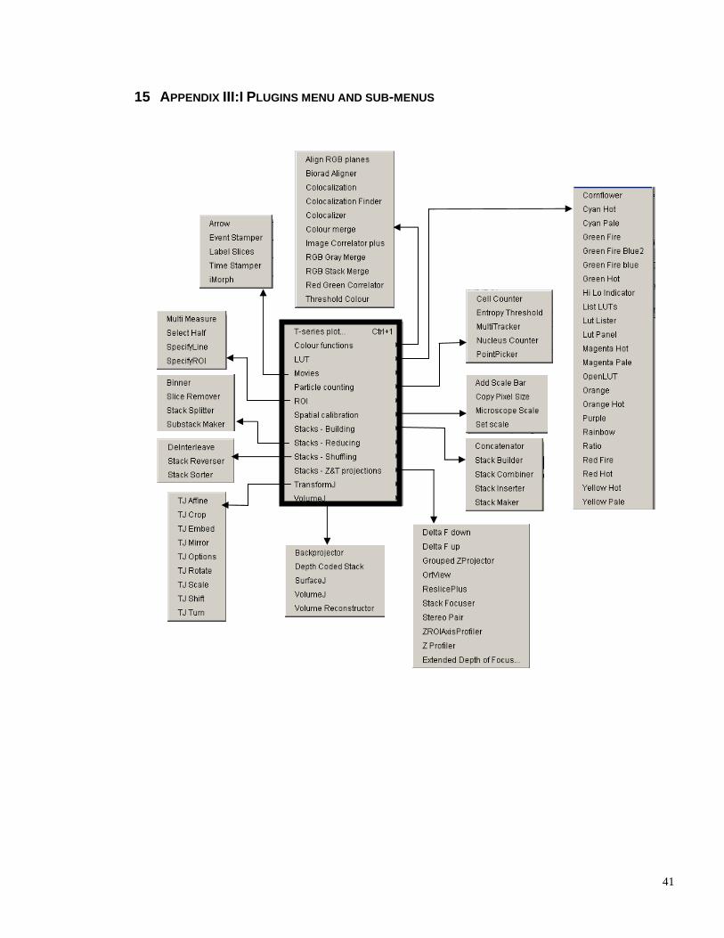
41

15 APPENDIX III:I PLUGINS MENU AND SUB -MENUS

42

16 APPENDIX IV: CUT OUT KEYBOARD TOOLBAR