irrigation & drainage engineering houndout adama university
TRANSCRIPT

Adama University, SOE & IT Irrigation and Drainage Engineering
Civil Eng’g & Architectures Department [surveying Engineering stream] By Tessema B. 1
Adama University School of Engineering and Information Technology Department of Civil Engineering and Architectures
Surveying Engineering Stream Course Title: Irrigation and Drainage Engineering [ CEng-4603]
Credit hour = 3 [Lec: 2hrs, Tut: 3hrs]
Prerequisite: CEng-2602[Hydraulics-II]
Objective This course enables the student to understand the b asic principles of design, construction and operation of the irrigation infrastructures. It als o assist to understand the need for drainage and the components out of which a drainage system is bu ilt up and provided them knowledge on the principles of Irrigation water management. Course Contents
1. INTRODUCTION 1.1. Definition of Irrigation 1.2. Necessity of Irrigation 1.3. Merit and Demerits of Irrigation 1.4. System of Irrigation 1.5 Irrigation Project Surveying 2. SOIL-WATER RELATIONSHIP 2.1 Basic soil -water relation 2.2 Soil Moisture Constants 2.3 Standard of Irrigation Water 2.4 Water quality testing of Irrigation Water 2.5 Rooting Characteristics and moisture Extraction Pattern 3. WATER REQUIREMENT OF CROPS 3.1 Consumptive use of water and various methods of determining it 3.2 Duty-delta relationship 3.3 Determination of irrigation water requirement of a crop 3.4 Depth of application and Frequency of irrigation 3.5 Irrigation efficiency 4. DESIGN OF IRRIGATION STRUCTURES 4.1 Design of Conveyances 4.2 Design of Diversion Structures 5. DESIGN OF DRAINAGES 5.1 Design of surface Drainage Systems 5.2. Design of Subsurface Drainage System 6. IRRIGATION METHODS 6.1 Surface Irrigation Systems 6.2 Pressurized Irrigation System Tentative Assessments 1. Assignments 10% 2. Midterm Exam 30% 3. Final Examination 60% Total 100% References: 1. Hydraulic Structure by P. Novak et'al 2. Irrigation Engineering by N.N Basak 3. Irrigation, Water Power and Water Resources Engineering by K.R ARORA 4. Design of Diversion Weirs by Rozgar Baban
Adama University, SOE & IT Irrigation and Drainage Engineering
Civil Eng’g & Architectures Department [surveying Engineering stream] By Tessema B. 2
CHAPTER ONE
1. INTRODUCTION 1.1 Definition of Irrigation • Irrigation is defined as:
o The process of artificial application of water to the soil for the growth of agricultural crop is termed as irrigation.
o It is particularly a science of planning and designing a water supply system for agricultural land to protect the crops from bad effect of drought or low rainfall.
• It includes the following structures for the regular supply of water to the required command area:
o the construction weir/barrage o dam/reservoir o canal system
1.2 Necessity of Irrigation For the growth of plant/crops: adequate quantity and quality of water required in the root zone of the plant. However, in actual condition during the whole period of plant growth /partly there exists inadequacy of water to full fill the crop water requirements. Thus, the following factors govern the necessity of irrigation: a) Insufficient rainfall: when the seasonal rainfall is less than the minimum requirement for the satisfactory growth of crops, the irrigation system is essential b) Uneven distribution of rainfall: when the rainfall is not evenly distributed during the crop period or throughout the cultivable area, the irrigation is extremely necessary. c) Improvement of perennial crops yield: some crops such as sugarcane etc require water through out the major parts of the year but the rainfall fulfills the demand during the rainy season only. Therefore, for remaining part of the year irrigation is necessary. d) Development of agriculture in the desert areas: in the desert, area where the rainfall is very scanty, irrigation is required for the development of agriculture. e) Insurance of drought: irrigation may not required during the normal rainfall condition and can be necessary during drought 1.3 Benefit and ill effect of Irrigation A. Direct Benefit of irrigation There are a number of benefits of irrigation and can be summarized as follows:
• Increase in crop yield • Protection of famine • Improvement of cash crops • Elimination of mixed cropping • prosperity of farmers • source of revenue • Overall development of the nation
B. Indirect Benefits of Irrigation • Hydroelectric development • flood control • domestic and industrial water supply

Adama University, SOE & IT Irrigation and Drainage Engineering
Civil Eng’g & Architectures Department [surveying Engineering stream] By Tessema B. 3
IRRIGATION SYSTEMS
Lift Irrigation
Flow Irrigation
Using man Or
Animal power
Using Mechanical Or
Electrical Power
Inundation Irrigation Perennial irrigation
Direct irrigation
Storage Irrigation
• navigation • development of fishery • ground water recharges Ill-effects of Irrigation The uses of irrigated agriculture have the following ill effects if not properly managed: • Raising of water Table • Formation of marshy area • dampness of weather • loss of soil fertility • soil erosion • production of harmful gases • loss of valuable lands 1.4 System of Irrigation The system of irrigation is classified as shown in the following charts
1.5 Method of Distribution of Irrigation Water After an irrigation water is taken from the sources by any of the techniques (Diversion from river or reservoir or pumped from the ground sources etc), it can be distributed to the agricultural field by different methods as summarized in the following chart schematically.

Adama University, SOE & IT Irrigation and Drainage Engineering
Civil Eng’g & Architectures Department [surveying Engineering stream] By Tessema B. 4
Method of Distribution
Surface Methods Sub-Surface Methods (Drip)
Sprinkler Methods Overhead Irrigation
Furrow Method
Contour Farming Methods
Flooding Methods
Uncontrolled Flooding
Controlled Flooding
Free Flooding Basin Flooding
Check Flooding
Border strip
A. Surface Method of Irrigation In this method, the irrigation method is distributed to the agricultural land through the small channels, which flood the area up to the required depth. The following figures show the schematic description of surface irrigation methods.

Adama University, SOE & IT Irrigation and Drainage Engineering
Civil Eng’g & Architectures Department [surveying Engineering stream] By Tessema B. 5
Adama University, SOE & IT Irrigation and Drainage Engineering
Civil Eng’g & Architectures Department [surveying Engineering stream] By Tessema B. 6
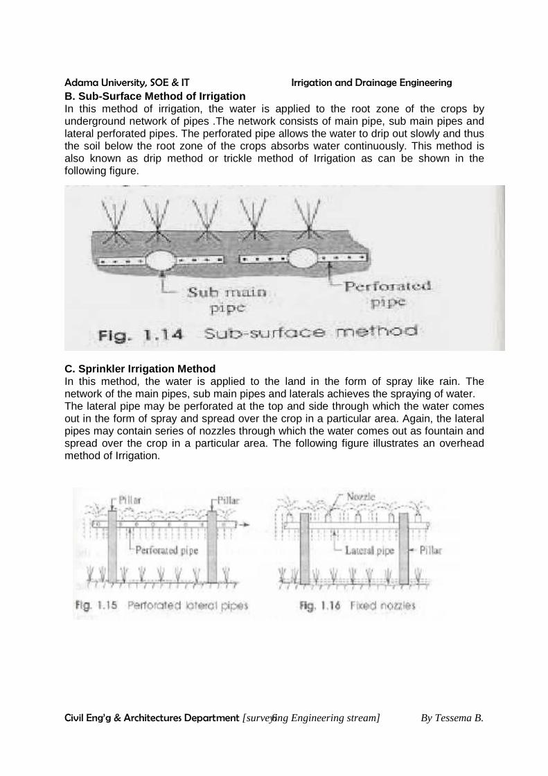
B. Sub-Surface Method of Irrigation In this method of irrigation, the water is applied to the root zone of the crops by underground network of pipes .The network consists of main pipe, sub main pipes and lateral perforated pipes. The perforated pipe allows the water to drip out slowly and thus the soil below the root zone of the crops absorbs water continuously. This method is also known as drip method or trickle method of Irrigation as can be shown in the following figure.
C. Sprinkler Irrigation Method In this method, the water is applied to the land in the form of spray like rain. The network of the main pipes, sub main pipes and laterals achieves the spraying of water. The lateral pipe may be perforated at the top and side through which the water comes out in the form of spray and spread over the crop in a particular area. Again, the lateral pipes may contain series of nozzles through which the water comes out as fountain and spread over the crop in a particular area. The following figure illustrates an overhead method of Irrigation.

Adama University, SOE & IT Irrigation and Drainage Engineering
Civil Eng’g & Architectures Department [surveying Engineering stream] By Tessema B. 7
1.6 Feasibility study or Irrigation project surveyi ng The data to be investigated during the feasibility study of a given irrigation project varies on the type of irrigation as well as its scope. Thus, any plan small or large, which ultimately aims at satisfying the paramount need of adequate water provision for crop production, is an irrigation project. Based on the scope of the irrigation project, irrigation projects can be classified as:
a) Large scale b) Medium scale c) Small scale
Irrigation projects and their development costs Type of project Command area
(ha) Development cost* U.S dollars/ha
Average cost Range in cost Large scale >10,000 16,000 5,000-50,000 Medium scale 2,000-10,000 9,000 4,000-15,000 Small scale <2,000 4,000 1,000-6,500
* Source: FAO, 1995. Note: In Ethiopia, Small-scale irrigations are those which have command areas <200 ha, medium scale 200-3000 ha and large scale >3000 ha.
With this respect, Ethiopia has a total potentially irrigable area of about 3,637,000 ha. , which is 27.55% of the total cultivable area. From which
o For small-scale irrigation 165,000-400,000 ha. o For medium and large scale irrigation 3,300,000 ha
1.6.1 Stages of investigations in the development o f irrigation projects:
♦ The development of water resources for irrigation requires the conception , planning , design , construction , and operation of various facilities to utilize and control water and to maintain water quality.
♦ Investigations of the development of irrigation projects need multi-disciplinary approach. Specialists of different disciplines, such as, Soil and water specialist, Engineers (Irrigation and civil), Agronomist, Geologist, and Socio-economist required.
♦ Investigations of water resources development projects are essentially aimed at collection of basic data and analysis thereof for formulation of an optimum project. The extent of data to be collected depends on the magnitude of the project and on the stage of investigation.
The common procedures adopted in the development of an irrigation project are:
1. Sites are located on the topographic-sheet. 2. The marked sites are inspected (reconnaissance) to decide their feasibility.

Adama University, SOE & IT Irrigation and Drainage Engineering
Civil Eng’g & Architectures Department [surveying Engineering stream] By Tessema B. 8
3. The feasibility investigations are carried out for one or more of the possible alternatives and estimates based approximate details are prepared.
4. Detailed investigations are then taken up and technical sanctions are granted. 5. After the technical sanction, agency of execution (i.e., contractor) is fixed and
construction started. Approaches of data collections: Before coming to the actual data collection for the feasibility study of any irrigation project, the following questions should be answered:
• What or which are the required data. • How they can be collected? • Why are they needed? • Is the cost of their collection worthwhile?
Feasibility studies of irrigation projects Through investigation of the following data are required during the feasibility study of an irrigation projects. • Necessity for irrigation in the region
o Normally Irrigation will be a necessity if there is inadequacy of rainfall, uneven distribution of rainfall, etc. On the other hand, it will be of a paramount importance to alleviate food shortage due to population growth.
• Availability of adequate water supply • Topography of the area • Cultural practices of the tract • Adequacy of existing irrigation system it any • Possibility of growing cash crops or other voluble crops after provision of irrigation
water • Accessibility to the project site (transportation, Communications and other required
facilities) and construction materials. • Economical justification for implementing the irrigation scheme. When the idea of an irrigation project is conceived (after reconnaissance survey), the data to be collected at the feasibility study stage are 1. Physical data: - location, size, physiographic (description of landform which includes
only physical aspects), climate, etc. 2. Hydrological data: Precipitation, Evaporation, transpiration, stream flow, sediment,
water quality etc. 3. Agricultural data: - land classification, crop water requirements, and types of crops 4. Geological data: - Rock & Soil types, ground water, minerals, erosion, etc. 5. Cartographic data: Topographic & other maps of the area. 6. Ecological data: - Types of vegetation, fish & wild life. 7. Demographic data: Population statistics, data of people etc. 8. Economic data: - Means of transportation, market, land taxes, etc. 9. Legal data: Water rights, land ownership and administrative pattern, etc 10. Data in existing project : - Types of Location of various projects. 11. Data on public opinion: - Opinions of different section of the society 12. Flood control data: Records of past flood, extent of damage caused by the flood,
drainage requirements etc
Adama University, SOE & IT Irrigation and Drainage Engineering
Civil Eng’g & Architectures Department [surveying Engineering stream] By Tessema B. 9
1.6.2 Land resources An evaluation of the suitability of land for alternative kinds of use requires a survey to define and map the land units together with the collection of descriptive data of land characteristics and resources. Land suitability is the fitness of a land-mapping unit for a defined use (in this case irrigation). Land mapping units represent parts of a study area (ex. for irrigation) which are more or less homogeneous with respect to certain land characteristics i.e. slope, rainfall, soil texture, soil type, etc). Land evaluation provides information and recommendations for deciding ‘which crops to grow where’ and related questions. Land evaluation is the selection of suitable land, and suitable cropping, irrigation and management alternatives that are physically and financially practicable and economically viable. The main product of land evaluation investigations is a land classification that indicates the suitability of various kinds of land for specific land uses, usually depicted on maps with accompanying reports. The four basic features of land suitability for irrigated agriculture are
• Irrigable terrain (land forms) • Potentially fertile soil • A climate in which the crop can thrive (develop well and be healthy) • A reliable source of water of consistent quality
The classification of the suitability of a particular land – mapping unit depends on the extent to which its land qualities satisfy the land use requirements. Definite specification (for land use requirements) is established for an irrigation project area prior to land classification. The land suitability classification requires the following information to be identified.
� Land capability maps are used to delineate arable and non-arable lands. � Land use and Vegetation maps of the catchments area are used to identify the
present land use in terms of cover and function. � Soil survey that includes:
• Identification of soil types • Field observation of infiltration • Field observation of hydraulic conductivity • Water table depth and fluctuation • Workability of the soil • Absence or presence of soil salinity
Soil survey recognizes the relation between terrain or physiographic and soils. Examples of: the minimum grade of a number of land qualities and land suitability ratings for irrigated rice.

Adama University, SOE & IT Irrigation and Drainage Engineering
Civil Eng’g & Architectures Department [surveying Engineering stream] By Tessema B. 10
Land qualities Land suitability rating S1 S2 Soil depth (cm) >60 >30 Soil fertility high low-medium Soil salinity (EC in mmhos/cm) <4 <8 Rock outcrops (% of ground surface) <2 <25 Net field water requirements (mm/day) <20 <20 Slope (%) <2 <4 Field size medium-large small Land development costs (US $ /ha <200 <600 Flooding nil or slight moderate
� Topographic Survey follows the soil survey and so is restricted mainly to the
areas of irrigable soils that have been delineated. Additional areas are included as necessary for the location of reservoir, dams, head works, canals, buildings, roads, and hydraulic structures etc.
1.6.3 Water resources Hydrological survey and Hydro-geological are undertaken to assess surface and sub-surface water resources of the catchments respectively. It may be carried out at national level, river basin level, project development level and at farm level. Data sources
� Surface water supply from long-term records of stream flows by stream gauging and water quality.
� If the above data is not available, rainfall records for the catchments or stream flow records of the neighboring rivers used.
� If the above two conditions did not exist, stream gauging and metrological stations are set up as soon as possible on the principle that having short-term records for correlation with homogenous gauged catchments which are better than none.
o For ground water supplies � Short-term yield is assessed by drilling and testing trial wells � Long-term yield is estimated by a detailed study of the aquifers � Mathematical models, numerical models that simulate the non-
steady state, two-dimensional, ground water flows are used for such purposes.)
1.6.4 Agricultural and Engineering aspects A. Agricultural Aspects
� In feasibility study, the present state of Agriculture and agricultural society is assessed and the future state, with irrigation, is predicted i.e. the ‘with’ and ‘without’ conditions of irrigation.
o Present farm practices o The number of farms of different sizes o Farming methods in use o Land areas cultivated and irrigated o Crop yield per hectare o Total crop production and costs

Adama University, SOE & IT Irrigation and Drainage Engineering
Civil Eng’g & Architectures Department [surveying Engineering stream] By Tessema B. 11
o Labor available for farming operation o Existing skill in irrigated farming and attitudes to change o Assessment on the existing market & transport o Presence of noxious weeds
o Future situation of agriculture. This assessment is much more difficult (numerous assumptions inevitably have to be made). It should be demonstrated that.
• The soils and the climate are suitable • The rotation of crops is sound • The water duties can be provided • There will be accessible markets capable of absorbing the increased production
at economic prices. • The advising and training facilities will be adequate, etc.
B. Engineering aspects � The Engineering aspect mainly focuses on the development of a source of water
for irrigation and construction of various structures for storage, diversion, conveyance and application of water. These includes investigations of : ♦ Site selection and Design of a reservoir & a dam ♦ Site selection & Design of diversion head – works at point off takes. ♦ Alignment for canal system (lay outs for canal) ♦ Alignment for field channels. ♦ Study of sub-surface conditions that affect the design and construction of
proposed structures. ♦ Concentrated on the mechanical properties of the sub soil at foundation
levels. ♦ Construction materials including, soil and sand, rock and aggregate, cement,
lime stone steel, etc. ♦ Tests should be carried out on the various construction materials. ♦ Any flood hazard so that provision of flood dyke protection is possible. ♦ If there is drainage requirements i.e. layouts of sub – surface drains. ♦ Other factors that have bearing effects upon the design of engineering works.
1.6.5 Social and Economical aspects. The attitude of the people to the introduction of irrigation in that area should be investigated thoroughly. The Various items considered in benefit/cost relationships are.
a) Costs � Capital cost of the project. � Cost of preliminary and precise survey and investigation � Cost of a equitation of land � Cost of various structures � Cost of earthwork and lining for canal system. etc � Allowance made for foreseen and unforeseen contingencies � Interest on Capital � Depreciation � Operational and maintenance cost of project

Adama University, SOE & IT Irrigation and Drainage Engineering
Civil Eng’g & Architectures Department [surveying Engineering stream] By Tessema B. 12
b) Benefits. � Agricultural production in the project area before and after taking up the
project (irrigation) � Cost of cultivation before and after irrigation (cost of inputs such as
Seeds, manure, labor, irrigation machines etc).
Then, B. C ratio = .Pr
.
ojectofCostAnnual
irrigationtoduebenefitannualNet
>1.5 for economically justified project. 1.6.6 Other Aspects to be considered:
o Organization and management aspects. o Further expansion potential of the project. o Environmental Surveys (Environmental Impact Assessment, EIA)

Adama University, SOE & IT Irrigation and Drainage Engineering
Civil Eng’g & Architectures Department [surveying Engineering stream] By Tessema B. 13
CHAPTER TWO
2. SOIL- PLANT -WATER RELATIONSHIPS Soil-plant Water relationships relate the properties of soil that affect the movement, retention and use of water. It can be divided & treated as:
� Soil-water relation � Soil-plant relation � Plant-water relations
2.1 Soil Suitability for agricultural practices Knowledge of the soils with in a potential irrigation area is essential for economic and technical reasons.
Definitions 1. A soil is a three-dimensional body occupying the upper part of the earth’s crust
and having properties differing from the underlying rock material as a result of interactions between climate, living organism, parent material and relief and which is distinguished from other soils in terms of differences in internal characteristics and/or in terms of the gradient slope- complexity, micro topography, stoniness, and rockiness of the surface.
2. Soil , superficial covering that overlies the bedrock of most of the land area of the
Earth; an aggregation of unconsolidated mineral and organic particles produced by physical, chemical, and biological processes; and the medium that supports the growth of most plants.
The primary components of soil are inorganic materials that are mostly produced by the weathering of bedrock; soluble nutrients, or chemical elements and compounds used by plants for growth; various forms of organic matter; and gases (notably oxygen, nitrogen, and carbon dioxide) and water required by plants and soil organisms.
Soil is an important natural resource and is the medium within which most agriculture takes place. The specific properties of soil are of great concern to farmers. Knowledge of the mineral and organic components of soils, of the amount of air they contain (aeration), and of their water-holding capacity, as well as of many other aspects of soil structure, is necessary for the successful production of crops.
Soil is a very important agricultural complement with out which no agricultural is possible. It is important to study the soil characteristics to say a particular soil type is suitable for agriculture or not. The process of the suitability of land for different uses such as agriculture is assessed and it is known as land evaluation. Land evaluation for agricultural purpose provides information for deciding ‘which crops to grow where’ and other related crops. Hence, before a land is put certain land uses, its suitability for that particular land use should be evaluated.
Adama University, SOE & IT Irrigation and Drainage Engineering
Civil Eng’g & Architectures Department [surveying Engineering stream] By Tessema B. 14
Soil map provides us with detailed information on soils that are utilized for land capability classification. This indicates the suitability or unsuitability of the soil for growing crops. Land capability classification is an interpretive grouping of soils based on inherent soil characteristics, external land features and environmental factors that may restrict the use of the land for growing varieties of crops. For land capability classification, we need information on: 1) The susceptibility of the soil to various factors that cause soil damage & decrease in
its productivity (we get this from soil map) 2) Its potential for crop production: Lands are first tentatively placed in different land
capability groups on the basis of slope of the land, erosion and depth of the soil. The suitability of soil for agricultural practices may be affected by physical and chemical soil characteristics. The physical characteristics include
1. Effective soil depth : - The depth of the soil, which can be exploited by crops, is very important in selecting soils for agricultural purpose. Experience has shown that many irrigated crops produce excellent yields with a well-drained effective root depth of 90 cm.
2. Water holding capacity: - This refers to the depth of water that can be held in the soil and available for plants. A good soil from agricultural point of view should have a very good water holding capacity. Clay soils have large water holding capacity, because drainage water is high in these soils. Ideally, loam soils are the best in this regard. Since in sandy soils an application loss are high and in clay soils drainage and aeration is difficult.
3. Non-capillary porosity : - High values of non- capillary porosity is desirable, because lower values of porosity and high values of bulk density hinders root development and expansion.
4. Topography : - A leveled land is the most suitable for agriculture. Because, the water for irrigation can easily be conveyed and less conservation and management practices are required. Where as, in sloppy soils, the more is the land wasted in bunds and channels in surface irrigation and there fore that cost for land development per unit area will be high.
5. Texture : - is the weight percentage of the mineral matters that occurs in each of the specified size fraction of the soil. It is the relative proportions of sand silt and clay, (Particles sized groups smaller than gravel i.e. < 2 mm in diameter). It is the number and sizes of its mechanical particles after all compounds holding them together have been destroyed. Loamy soils are the best texture for agriculture. Deviation either into sandy or clayey texture will reduce the value of the land for agriculture.
6. Soil Structure: It refers to the manner in which primary soil particles are arranged into, secondary particles or aggregates. Soil structure determines the total porosity, the shape of individual pores and their size distribution, hence it affects: -
• Retention & transmission of fluids in the soil • Germination • root growth • Tillage • Erosion etc.

Adama University, SOE & IT Irrigation and Drainage Engineering
Civil Eng’g & Architectures Department [surveying Engineering stream] By Tessema B. 15
7. Soil Consistence: Is the resistance of the soil to deformation or rupture. It is determined by the cohesive and adhesive properties of the entire soil mass. Structure deals with size, shape and distinctness of natural soil aggregates, and consistence deals with strength and nature of the force between particles. It is important for tillage or traffic consideration.
Soil Consistence Terms : - Consistence is described for three-moisture levels i.e. wet, moist & dry. For instance, a given soils may be sticky when wet, firm when moist and hard when dry. The terms to describe soil consistency include - 1) Wet soil - non sticky, sticky, non plastic, plastic 2) Moist soil - loose, friable, firm 3) Dry soil - loose, soft, and hard. 8. Soil Permeability and Hydraulic Conductivity Permeability - is the ease with which liquids, gases and roots pass through the soil. Hydraulic conductivity is the permeability of the soil for water. I.e. the ease with which the soil pores permit water movement. It controls the soil water movement.
The major factors affecting hydraulic conductivity are texture and structure of soils. E.g., Sandy soils have higher saturated conductivity than finer textured soils. Soils with stable granular structure conduct water rapidly than those with unstable structural units, since they will not break down when get wetted. Fine textured soils during dry weather because of their cracks allow water rapidly then the cracks swell shut, and drastically reduce water movement. 1. Salinity (soluble salt content) When the quantity of salts in irrigated land is too high, the salts accumulate in the crop root zone. These salts create difficulty to crops in extracting enough water from the salty solution. Thus, for the land to be of high value for irrigation, the soluble salt content should be low as much as possible. 2. Amount of Exchangeable sodium:- When the amount of exchangeable sodium is high in the soil, the soil will have large amount of Na+ in the form of colloid. This results in tremendous reduction of the permeability of the soil. This in turn makes it difficult to the cop to get sufficient water and causes crusting of seedbeds. Such a soil is called Black alkali soil. Hence, the amount of exchangeable sodium should be low in agricultural lands. 3. Soil Reaction (PH): is a measure of its acidity or alkalinity. It is a measure of the concentration of hydrogen ion in a soil. Mathematically,
= + )(
1log10 H
PH
Excessively low or high pH values are not good for proper growth and adequate yield production as they bring about acidity or alkalinity in the soil. In general, in any ecosystem, (a farm, forest, regional water shed etc.) soils have five key roles
1. Medium for plant growth: It supports the growth of higher plants by providing a medium for plant roots and supplying nutrient elements that are essential to the entire plant.
Adama University, SOE & IT Irrigation and Drainage Engineering
Civil Eng’g & Architectures Department [surveying Engineering stream] By Tessema B. 16
2. Regulator of water supplies: Its properties are the principal factor controlling the fate of water in the hydrologic system. Water loss, utilization, contamination, and purification are all affected by the soil.
3. Recycler of raw materials: With in the soil, waste products and dead bodies of plants, animals and people are assimilated, and their basic elements are made available for reuse by the next generation of life.
4. Habitat for soil organisms: It provides habitats for living organism, from small mammals and reptiles to tiny insects to microscopic cells.
5. Engineering medium: In human - built ecosystem, soil plays an important role as an engineering medium. It is not only an important building material (earth fill, bricks) but provides the foundation for virtually every road, airport, and house we build. In relation to irrigation:
• The capacity of the soil to accept, transmit or retain relatively large amounts of water (Water holding capacity of the soil) in a relatively large amounts of water in a relatively short time should be measured.
• The surface infiltration rates and the case of water movement through unsaturated and through saturated layers (hydraulic conductivity) need to be measured punitively.
� The amount, kind and distribution of clay minerals (Soil chemical properties) are especially important to water movement, relation and availability of plants.
• Studies of cracking and structural changes under different management Practices (helps surface sealing or a need of pre irrigation) and
� Physical properties of soil matrix. 2.2 Soil- water relations
� It means that physical properties of soil in relation to water � The rate of entry of water in to the soil and its retention, movement and
availability to plant roots are all physical phenomena. Hence, it is important to know the physical properties of soil in relation to water.
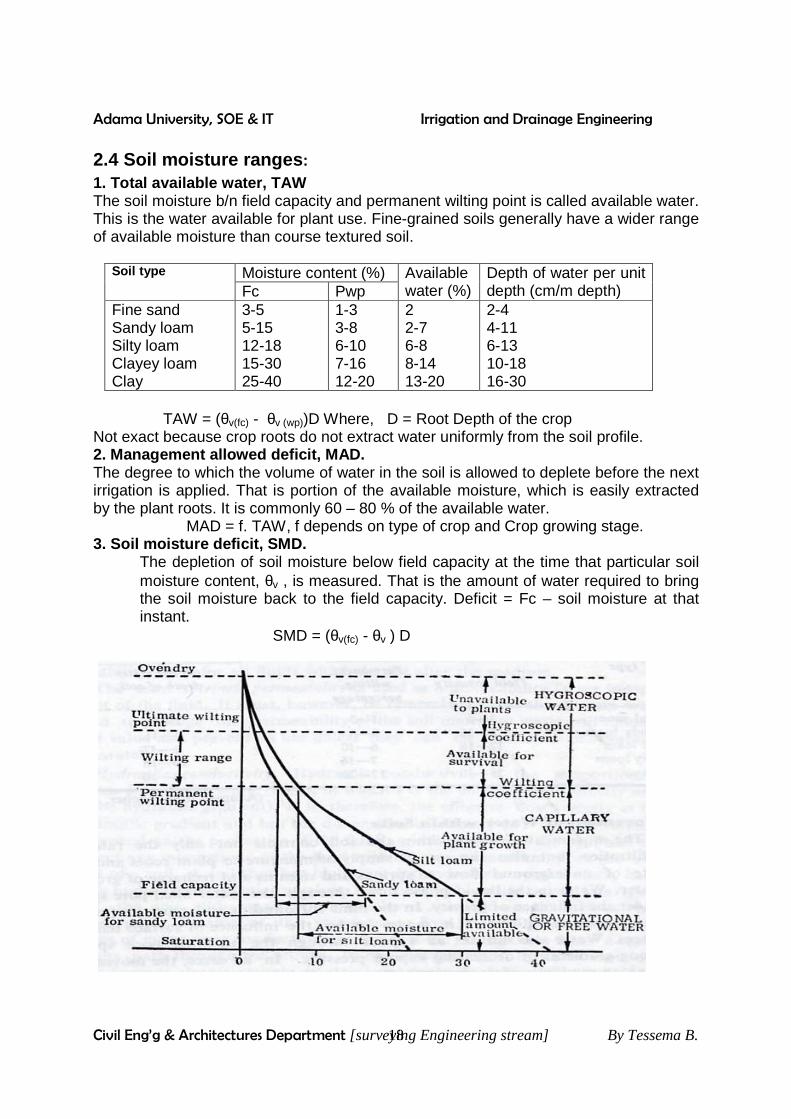
2.3 Classes of Soil Water Availability Water can exist in either of the following forms in the soil. Gravitational water: Water is rapidly drained from the soil profile by the force of gravity. The term rapid is relative and in soil-water studies normally refers to periods of 24 to 48 hours. Capillary water: is the water remaining after rapid drainage by gravity that can require force greater than gravity such as those exerted by plant roots may remove this water. Hygroscopic water: the water that is forces generally found in nature, adheres to soil particles, cannot be removed from the soil particles by the plant roots. Hygroscopic water can be removed by oven drying a soil sample in the laboratory. Water may also be classified as unavailable, available and gravitational or superfluous. Such a grouping refers to the availability of soil water to plants. Gravitational water drains quickly from the root zone under normal drainage conditions. Unavailable water is held too tightly by capillary forces and is generally not accessible to plant roots. Available water is the difference between gravitational and unavailable water.

Adama University, SOE & IT Irrigation and Drainage Engineering
Civil Eng’g & Architectures Department [surveying Engineering stream] By Tessema B. 17
Water drains from the soil under the constant pull of gravity. Sandy soils drain rapidly, while clay soils drain very slowly. Hence, one day after irrigating a sandy soil has drained most of the gravitational water, where as clay may require four or more days for gravitational water to drain. 2.4 Soil Moisture Constants The following soil moisture contents are of significance importance in agriculture and are termed soil moisture constants. 1. Saturation Capacity : - When all the micro and macro pore spaces are filled with
water, the soil is said to have reached its saturation capacity. At field capacity, the water is held loosely and tensions are almost negligible. Thus, plants will not have any difficulty in extracting moisture from soil.
2. Field capacity : - is the moisture content after the gravitational water has drained down. At field capacity, the macro pores are filled with air & capillary pores filled with water. Field capacity is the upper limit of available soil moisture. It is often defined as moisture content in a soil two (light sandy soil) or three (heavy soil), days after having been saturated and after drainage of gravitational water becomes slow or negligible and moisture content has become stable.
- Larger pore spaces filled with air while the smaller ones with water - At field capacity, Soil Moisture Tension (SMT) is b/n 1/10 – 1/3 atm .
Some of the factors, which influence the field capacity of the soil, are soil texture and presence of impending layer (soil profile), arise from plaguing the same depth yearly ⇒ hard pan. The volumetric moisture content at field capacity is given by: θfc = ρ b. θm Field capacity can be determined by ponding water on a soil surface in an area of about 2 to 5 m2 and allowing it to drain for one to three days preventing surface evaporation. Then soil samples are taken from different depths and the moisture content is determined as usual, which gives the field capacity. 3. Permanent Wilting Point : - is the moisture content beyond which plants can no
longer extract enough moisture and remain witted unless water is added to the soil. The water beyond the permanent wilting point is tightly held to the solid particles that plants cannot remove moisture at their normal rate to prevent wilting of the plants. The soil moisture tension at PWP ranges from 7 to 32 atm, depending on the soil texture, kinds of crops and salt content in the soil solution.
- Since the change in moisture content (∆θ) is insignificant for changes in SMT from 7-32 atm. Hence, 15 atm. is taken as SMT at PWP.
- At PWP the plant starts wilting, and if no water is given to the plant, then it will die.
N. B θv(wp) = ρb θm(wp) (volumetric moisture content at Permanent wilting point)
Adama University, SOE & IT Irrigation and Drainage Engineering
Civil Eng’g & Architectures Department [surveying Engineering stream] By Tessema B. 18
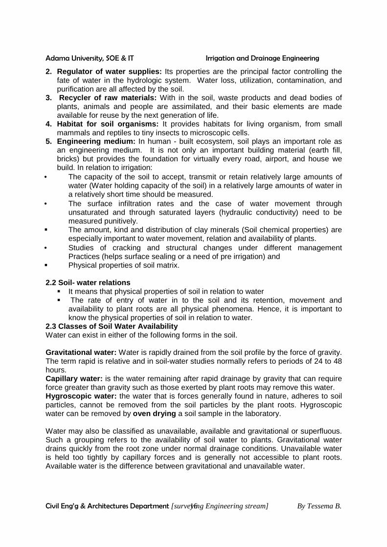
2.4 Soil moisture ranges : 1. Total available water, TAW The soil moisture b/n field capacity and permanent wilting point is called available water. This is the water available for plant use. Fine-grained soils generally have a wider range of available moisture than course textured soil.
Soil type Moisture content (%) Available water (%)
Depth of water per unit depth (cm/m depth) Fc Pwp
Fine sand Sandy loam Silty loam Clayey loam Clay
3-5 5-15 12-18 15-30 25-40
1-3 3-8 6-10 7-16 12-20
2 2-7 6-8 8-14 13-20
2-4 4-11 6-13 10-18 16-30
TAW = (θv(fc) - θv (wp))D Where, D = Root Depth of the crop
Not exact because crop roots do not extract water uniformly from the soil profile. 2. Management allowed deficit, MAD. The degree to which the volume of water in the soil is allowed to deplete before the next irrigation is applied. That is portion of the available moisture, which is easily extracted by the plant roots. It is commonly 60 – 80 % of the available water.
MAD = f. TAW, f depends on type of crop and Crop growing stage. 3. Soil moisture deficit, SMD .
The depletion of soil moisture below field capacity at the time that particular soil moisture content, θv , is measured. That is the amount of water required to bring the soil moisture back to the field capacity. Deficit = Fc – soil moisture at that instant.
SMD = (θv(fc) - θv ) D
Adama University, SOE & IT Irrigation and Drainage Engineering
Civil Eng’g & Architectures Department [surveying Engineering stream] By Tessema B. 19
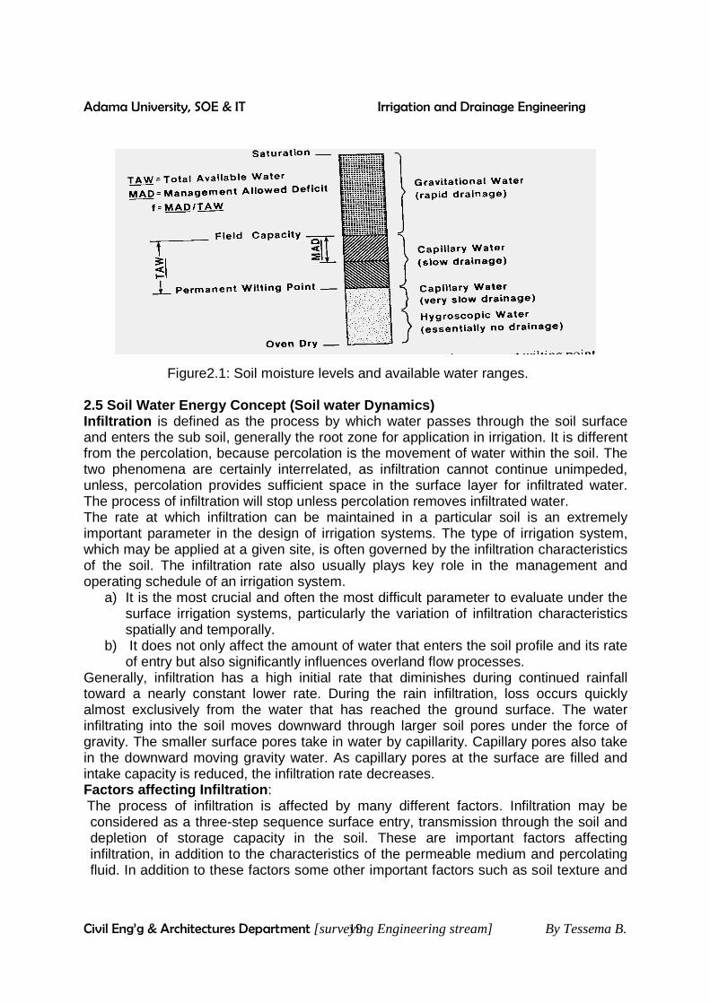
Figure2.1: Soil moisture levels and available water ranges. 2.5 Soil Water Energy Concept (Soil water Dynamics) Infiltration is defined as the process by which water passes through the soil surface and enters the sub soil, generally the root zone for application in irrigation. It is different from the percolation, because percolation is the movement of water within the soil. The two phenomena are certainly interrelated, as infiltration cannot continue unimpeded, unless, percolation provides sufficient space in the surface layer for infiltrated water. The process of infiltration will stop unless percolation removes infiltrated water. The rate at which infiltration can be maintained in a particular soil is an extremely important parameter in the design of irrigation systems. The type of irrigation system, which may be applied at a given site, is often governed by the infiltration characteristics of the soil. The infiltration rate also usually plays key role in the management and operating schedule of an irrigation system.
a) It is the most crucial and often the most difficult parameter to evaluate under the surface irrigation systems, particularly the variation of infiltration characteristics spatially and temporally.
b) It does not only affect the amount of water that enters the soil profile and its rate of entry but also significantly influences overland flow processes.
Generally, infiltration has a high initial rate that diminishes during continued rainfall toward a nearly constant lower rate. During the rain infiltration, loss occurs quickly almost exclusively from the water that has reached the ground surface. The water infiltrating into the soil moves downward through larger soil pores under the force of gravity. The smaller surface pores take in water by capillarity. Capillary pores also take in the downward moving gravity water. As capillary pores at the surface are filled and intake capacity is reduced, the infiltration rate decreases. Factors affecting Infiltration : The process of infiltration is affected by many different factors. Infiltration may be considered as a three-step sequence surface entry, transmission through the soil and depletion of storage capacity in the soil. These are important factors affecting infiltration, in addition to the characteristics of the permeable medium and percolating fluid. In addition to these factors some other important factors such as soil texture and

Adama University, SOE & IT Irrigation and Drainage Engineering
Civil Eng’g & Architectures Department [surveying Engineering stream] By Tessema B. 20
structure, condition at soil surface; soil - moisture content, type of vegetative cover, soil temperature, Human activities on soil surface, may also affect the infiltration.
1. Surface entry : The surface of the soil may be sealed by the in wash of fines or other arrangements of particles that prevent or retard the entry of water into the soil. Soil having excellent under drainage may be sealed at the surface and there by have a low infiltration rate. 2. Transmission through the soil : Water cannot enter the soil more rapidly than it is transmitted downward. Conditions at the surface cannot increase infiltration unless the transmission capacity of the soil profile is adequate. 3. Depletion of Available Storage Capacity in the s oil: the storage available in any horizon depends on porosity, thickness of the horizon and the amount of moisture already present. Texture structure, organic matter content, root penetration colloidal swelling, and many other factors determine the nature and magnitude of the porosity of the soil horizon. Total porosity as well as the size and arrangement of pores, has a significant bearing upon the availability of storage. The volume will largely control the infiltration that occurs in the early part of the storm, sizes and continuity of non-capillary or large pores because such pores provide easy paths for the movement of percolation water. 4. Characteristics of the permeable medium : Factors that affect infiltration are the characteristics of the permeable medium. The soil and the characteristics of the percolating fluid are of significant importance. In soil the problems concerns it self largely with pore size and pore - size distribution that is the proportion of different sizes present, as well as their relative stability during storms, irrigations, or other applications of water. In sands, the pores are relatively stable, since the sand particles that form, they are not readily disintegrated, nor do they swell upon wetting. During a storm or irrigation, they may rearrange themselves into a more dense mix than formerly. However, this change in condition of the sand is relatively slow when compared with changes that occur in silts or clays. 5. Characteristics of the fluid : Another group of factors that affect infiltration though usually to a lesser degree is those modify the physical characteristics of the fluid namely; water pure rainwater enters the soil. The infiltrating fluid is often contaminated by the salts, particularly in the alkali soils, and to some extent in many other soils. These salts may affect the viscosity of the fluid and form complexes with the soil colloids, which affect the welling rate when wet. Irrigation water very often contains residues of fertilizer, particularly when they are reused. Water in farm ponds may contain impurities that modify infiltration. 6) Soil Texture and Structure : The water cannot continue to enter soil more rapidly than it is transmitted downward. Therefore, the conditions at the surface cannot increase infiltration unless the transmission capacity of the soil profile is adequate. The continuity of non-capillary or large pores provides easy paths for percolating water. If the sub soil formation has coarse texture, the water may infiltrate into the soil so quickly that no water will be left for runoff even if rainfall is quite heavy. On the contrary, clayey soils after soaking some water in the initial stages of rainfall may swell considerably. It makes the soil almost watertight and infiltration may be reduced to practically negligible extent.

Adama University, SOE & IT Irrigation and Drainage Engineering
Civil Eng’g & Architectures Department [surveying Engineering stream] By Tessema B. 21
7) Conditions at soil surface : Even if the soil has excellent under- drainage but at the surface, soil pores are sealed due to turbid water or by in wash. These soil particles may prevent entry of water into the soil and infiltration rate will be low. 8) Soil- moisture content : When the soil is dry the rate of infiltration into the soil is very high. The infiltration rate diminishes as the soil - moisture storage capacity is exhausted. After this infiltration rate equals transmission rate. The rate of infiltration in early phases of a rainfall will be less if the soil pores are still filled from previous rainstorm. Measurement of infiltration: Due to the complexity of the infiltration phenomenon and the fact that many factors affect the process, the measurements of infiltration rates and volumes should be accomplished under field conditions. Infiltration can be measured by two methods namely (1) indirect method or by infiltrations (2) Direct method Hydrograph analysis. 1. Indirect Method: They involve artificial application of water over sample area. The mechanism used for this purpose is called infiltration. There are two types of infiltrometers such as flooding type and rain simulators 2. Direct method: It consists of analysis of runoff hydrograph resulting from a natural rainfall over a basin under consideration. The following figure illustrates the characteristics of infiltration for different type of soils and the initial soil moisture contents.
Fig.2.2 Example of Infiltration rate (Average, instantaneous), and cumulative infiltration depth

Adama University, SOE & IT Irrigation and Drainage Engineering
Civil Eng’g & Architectures Department [surveying Engineering stream] By Tessema B. 22
Time (h) Fig2.3: Infiltration rate as function of moisture content
Generally the following factors limits infiltration rate: • initial (antecedent) moisture content • conditions of sub-soil • hydraulic conductivity of the soil profile • texture, porosity (changed by cultivation and compaction) • Degree of swelling of soil colloids and organic matter • Vegetation cover, duration of rainfall or irrigation
2.6 CHARACTERISTICS OF MAJOR SOILS in Ethiopia In Ethiopia Lithosols, Nitosols, cambisols. Regosls , Vertisols and Fluvisols cover approximately 17.2%, 12.2%, 11.6% 10.9%, and 8.3% of the total land area of the country. When only arable lands are considered Nitosols, Cambisols and Vertisols are the major soil types and occupy nearly 23%, 195 and 18% of the total area respectively. However the exact characteristics and distribution of the Ethiopian soils are still not fully documented and mapped yet (LUPRD, 1986) The latest soil map of Ethiopia, which had been developed from the FAO/UNESCO soil map of the world at a scale of 1:2,000,000 and the nomenclature of FAO/UNESCO system is used to classify the soils. Only soils that occur in significant amount are explained here. Lithosols: These soils are less than 10 cm deep and could be young or have resulted from seyere erosion. Lithosols have low water holding capacity and they are found on steep slopes. They could occur under any sub agro-ecological zone but mainly in the Northern regions of the country (Tigray, Wello, Gonder, Northern Shewa, Ogaden) on steep slopes and mountainous or hilly areas.

Adama University, SOE & IT Irrigation and Drainage Engineering
Civil Eng’g & Architectures Department [surveying Engineering stream] By Tessema B. 23
Nitosols: These soils are deep (>150cm). reddish brown clays and mostly occur form sub-moist to humid agro-ecological zones of mainly the western and southern parst of the country (Wellega, illubabor,Keffa, Jimma, Sidamo, Southern Shewa and parts of Gojjam).Nitosols are highly weathered, acidic high p-fixing and well drained soils. These soils are productive with proper fertilization and management, but are vulnerable to leaching and erosion. With increasing acidity Nitosols may be converted to Acrisols. Cambisols : Cambisols are soils occurring mostly in steep slopes where erosion is common. These soils have large variation being either acidic or basic, so are highly productive while others may be poor in fertility. They may occur in many agro-ecological sub-zones but mostly in the North Eastern rift valley escarpments. Regosols: These soils are developed from unconsolidated materials and occur under different agro-ecological sub-zones although more commonly in the drier areas of eastern part of the country. They are poor in phosphorous. Vertisols: are clay soils with black to gray colour having high swelling and shrinking capacity. Poor drainage when wet and cracking when dry is the characteristic of Vertisols and difficult to work. Vertisols are common in the central plateau of the country (Gojjam, Shewa, Arsi, Bale, in the bottomlands of Garerge highlands, and in Gambella. They are productive if drainage problem can be improved.) Fluvisols: These soils were developed from recent alluvium, are very fertile, and occur on that ground at the bottom valleys along the sides of streams. Fluvisosls often have drainage problem but the making of number beds for the main season use can alleviate the problem. They are very productive if used in the off-season with irrigation or in the small rainy season. Xerosols: These soils occur in the semi-arid regions have low organic matter content and are likely high in salinity. They have also phosphorous, magnesium, potassium, iron, zinc, and high in gypsum. Acrisots Acrrsols are old soils that have lost most of the bases because of leaching. Hence, they are acidic and highly P-fixing type and mostly occur in the sub-humid and humid regions of western and southern Ethiopia. Types of soils Ne Eutric Bitosols
Percentage coverage 5
Agricultural potential, Best Soils
Nd, Dystric Bitosols 7.6 Good potential L. chromic & Orthic Luvisols
5 Good potential
BV. Vertic Cambisols & Luvisols
3 Fairly Good potential
J. Calcaric & Eutric Fluvisols
8.5 Good potential
T. Humic, Molic & Vitric Andosols
1 Good potential
V. chromic & pellic Vertisosls
10 Good potential
A. orthic Acrisols 4.5 Limited potential Q. calcic Arenoslos 5 Limited potential R. Calcaric & Eutric 11 Limited potential

Adama University, SOE & IT Irrigation and Drainage Engineering
Civil Eng’g & Architectures Department [surveying Engineering stream] By Tessema B. 24
Regosols X. Halpic, Calcic & Luvic Xersols
5 Limited potential
Bh. Dystric & HGumic Cambisols
2 Not important
H.Haplic & Luvie 4 Not important Lithosols 17 Not important Y.Gypsic Yermosols 3 Not important Z. Gleyic & Orthic solon-Chalks
5 Saline soils
Source: National Atlas of Ethiopia (1988) 2.7 PRINCIPAL CROPS OF ETHIOPIA The highlands constituting 47% of the total area of the country accommodate 74% of the population. The total cultivated land is about 14% of the total area of the country: 93% of this is used for food production. This is, of course, not surprising since we are dealing with subsistence farming. The former Shewa administrative region, the most intensively cultivated of all, accounts for 24% of the cultivated land and 26% of the total food crop production. Southwestern Ethiopia (former Keffa, Illubabor, and Western Wellega) with elevations ranging from 1500m to 2400m receives the highest rainfall in the country. Maize is by far the most important food crop representing between 40-50% of the total food production of the region.
The eastern highlands, stretching across the administrative regions of Sidamo, Bale, Arsi, and Harerge, have altitudes above 1800 m with average annual rainfall ranging from 950 mm to 1500mm. 16% of the cultivated land and 19% of the total production is found in this region. In sidamo more than 60% of the total food production is maize. In Arsi and Bale, wheat and barley are the two most dominant food crops. In Harerge more than 60% of the total food production is Sorghum, followed by maize, 23%. The major food crops produced in the country are cereals, pulses and oilseeds. Cereal crops occupy the largest area (86%) of the food crops. Important cereal crops are Teff (Eragrostis Tef), wheat, barley, sorghum, maize and millet. Theses can be categorized into two groups, the cool weather and the warm weather crops. Teff, wheat and barley are cool weather crops. They are grown on the highlands above 1500m where the average annual temperature ranges between 160 C and 200c, and where the annual rainfall varies from 800 mm to 1500 mm they grow under a wide variety of soil conditions. Teff, sorghum, maize and barley are the most widely grown and represent 73% of the food crops. Teff is considered the most important food crop in Ethiopia. Of the food crops, it has the largest total production (19.8%) and occupies the largest area (24.3%). It is the most preferred food crop in most parts of highland Ethiopia. The major crops produced under irrigation in Ethiopia are cotton, sugar cane, fruits vegetables, and to some extent cereals. From the total area under irrigation in 1988/89,

Adama University, SOE & IT Irrigation and Drainage Engineering
Civil Eng’g & Architectures Department [surveying Engineering stream] By Tessema B. 25
about 46 and 17 thousand ha is covered by cotton and sugar cane, respectively, while irrigation contributed about 3% of the total production of cereals. 2.8 CROP ROTATION PRACTICES When the same crop is grown repeatedly in the same field, the fertility of land is reduced, as the soil becomes deficient in plant foods favorable to that particular crop. In order to enhance the fertility of the land and to make soil regain its original structure, it is often found necessary and helpful to give some rest to the land. This can be achieved either by allowing the land to lie fallow without any cultivation for some time, or to grow crops which do not mainly require those salts or foods which were mainly required by the earlier grown crop. This method of growing different crops in rotation one after the other in the same field is called crop rotation. A cash crop may be followed by a fodder crop, which in turn may be followed by a soil-renovating crop. The rotation of crops will help in extracting different foods from the soil, and thus avoiding the general deficiency of any particular type. Moreover, if only one type of crop is grown in the same field. Numerous insects and pests (of similar nature) will get developed. The crop rotation will also help in checking such growths Crop rotation will thus help in increasing the fertility of soil, and reducing the diseases and wastages due to insects and hence increasing overall crop yield. Using leguminous crops in rotation helps in giving nitrogen to the fields. There could be deep-rooted crops and shallow rooted crops in rotation and so they shall draw their food from different depths of soil.

Adama University, SOE & IT Irrigation and Drainage Engineering
Civil Eng’g & Architectures Department [surveying Engineering stream] By Tessema B. 26
CHAPTER THREE
3. CROP WATER REQUIREMENTS 3.1 Duty-Delta relation ship Duty of water: is its capacity to irrigate land. It is the relation between the area of the land irrigated and the quantity of water required. Thus, Duty (D) is defined as the area of the land, which can be irrigated if one cumec (m3/sec) of water was applied to the land continuously for the entire base period of the crop and it is expressed in hectares / cumecs.
Base period (B): the base period is the period between the first watering and the last watering. The base period is slightly different from the crop period, which is the period between the time of sowing and the time of harvesting the crop. Delta ( ): is the total depth of water required by a crop during the entire base period. If the entire quantity of applied water were spread uniformly on the land surface, the depth of water would have been equal to delta. Thus the delta (in m) of any crop can be determined by dividing the total quantity of water (in ha-m) required by the crop by the area of the land (in ha) Delta ( ) = Total quantity of water (ha-m)
Total area of land (ha) The relation between duty, base period and delta, can be obtained as follows. Considering the area of land of D-hectares and If Duty is expressed in ha/cumecs the total quantity of water used in the base period of B days is equal to that obtained by a continuous flow of 1 cumec for B days. Quantity of water= 1*B*24*60*60*, m3 ------------------------------------------------ (a) If Delta ( ) is the total depth of water in meters supplied to the land of D- hectares, the quantity of water is also given by: Quantity of water = (D *104)* m3 -------------------------------------------------- (b) Equating the volumes of water given in egn_s (a) and (b) 1*B*24*60*60* = (D*104)* � D = 8.64 B = 8.64B D Where D = in ha/cumec = In m B = in days

Adama University, SOE & IT Irrigation and Drainage Engineering
Civil Eng’g & Architectures Department [surveying Engineering stream] By Tessema B. 27
Factors affecting Duty - Duty of water depends up on different factors. In general, the smaller the losses,
the greater are duty because one cumec of water will be able to irrigate larger area.
� Type of soil � Type of crop and base period � Structure of soil � Slop of ground � Climatic condition � Method of application of water � Salt content of soil
Counteracting all the factors that decrease the duty by decreasing various losses may improve duty of water. Example: The base period, duty of water and area under irrigation for various crops under a canal system are given in the table below. If the losses in the reservoir and canals are respectively 15%, 25%, determine the reservoir capacity.
Solution_ = Calculation is tabulated here below.
Total volume of water 47,910 ha-m
Volume at head of canal = 880,6375.0
47910= ha-m
Volume of reservoir = 150,7585.0
63880= ha-m
Crop Wheat Sugar cane
Cotton Rice V. table
Base period B (days) 120 320 180 120 120 Duty, D (ha/cumec) 1800 1600 1500 800 700 Area irrigated (ha) 15000 10,000 5000 7500 5000
Crop Wheat Sugarcane cotton Rice Veg. Sum
∆= mD
B,
64.8
0.576
1.725
0.972
1.296
1.481
-
Volume of water
∆*Airr (ha-m)
8640
17280
4860
9720
7410
47910 ha-m
Adama University, SOE & IT Irrigation and Drainage Engineering
Civil Eng’g & Architectures Department [surveying Engineering stream] By Tessema B. 28
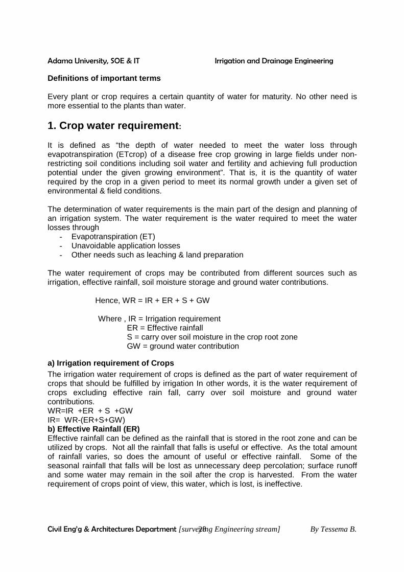
Definitions of important terms Every plant or crop requires a certain quantity of water for maturity. No other need is more essential to the plants than water.
1. Crop water requirement : It is defined as “the depth of water needed to meet the water loss through evapotranspiration (ETcrop) of a disease free crop growing in large fields under non-restricting soil conditions including soil water and fertility and achieving full production potential under the given growing environment”. That is, it is the quantity of water required by the crop in a given period to meet its normal growth under a given set of environmental & field conditions. The determination of water requirements is the main part of the design and planning of an irrigation system. The water requirement is the water required to meet the water losses through
- Evapotranspiration (ET) - Unavoidable application losses - Other needs such as leaching & land preparation
The water requirement of crops may be contributed from different sources such as irrigation, effective rainfall, soil moisture storage and ground water contributions. Hence, WR = IR + ER + S + GW Where , IR = Irrigation requirement ER = Effective rainfall S = carry over soil moisture in the crop root zone GW = ground water contribution
a) Irrigation requirement of Crops The irrigation water requirement of crops is defined as the part of water requirement of crops that should be fulfilled by irrigation In other words, it is the water requirement of crops excluding effective rain fall, carry over soil moisture and ground water contributions. WR=IR +ER + S +GW IR= WR-(ER+S+GW) b) Effective Rainfall (ER) Effective rainfall can be defined as the rainfall that is stored in the root zone and can be utilized by crops. Not all the rainfall that falls is useful or effective. As the total amount of rainfall varies, so does the amount of useful or effective rainfall. Some of the seasonal rainfall that falls will be lost as unnecessary deep percolation; surface runoff and some water may remain in the soil after the crop is harvested. From the water requirement of crops point of view, this water, which is lost, is ineffective.

Adama University, SOE & IT Irrigation and Drainage Engineering
Civil Eng’g & Architectures Department [surveying Engineering stream] By Tessema B. 29
People in different disciplines of course define effective rainfall in different ways. For instance to a canal irrigation engineer, it is the rainfall that reaches the storage reservoir, to a hydropower engineer, it is the rainfall that is useful for running the turbines and for Ground water engineers or Geo – hydrologists, it is that portion of the rainfall that contributes to the ground water reservoir. CropWat 4 Windows has four methods for calculating the effective rainfall from entered monthly total rainfall data. 1. Fixed Percentage Effective Rainfall The effective rainfall is taken as a fixed percentage of the monthly rainfall: Effective Rainfall = % of Total Rainfall 2. Dependable Rain An empirical formula developed by FAO/AGLW based on analysis for different arid and sub-humid climates. This formula is as follows: Effective Rainfall = 0.6 * Total Rainfall - 10 (Total Rainfall < 70 mm) Effective Rainfall = 0.8 * Total Rainfall - 24 (Total Rainfall > 70 mm) 3. Empirical Formula for Effective Rainfall This formula is similar to FAO/AGLW formula (see Dependable Rain method above) with some parameters left to the user to define. The formula is as follows: Effective Rainfall = a * Total Rainfall - b (Total Rainfall < z mm) Effective Rainfall = c * Total Rainfall - d (Total Rainfall > z mm) Where a, b, c, and z are the variables to be defined by the user. 4. Method of USDA Soil Conservation Service (defaul t) The effective rainfall is calculated according to the formula developed by the USDA Soil Conservation Service, which is as follows: Effective Rainfall = Total Rainfall / 125 * (125 - 0.2 * Total Rainfall) (Total Rainfall < 250 mm) Effective Rainfall = 125 + 0.1 * Total Rainfall (Total Rainfall > 250 mm) c) Ground water contribution (GW): Some times, there is a contribution from the groundwater reservoir for water requirement of crops. The actual contribution from the groundwater table is dependent on the depth of ground water table below the root zone & capillary characteristics of soil. For clayey soils, the rate of movement is low and distance of upward movement is high while for light textured soils, the rate is high and the distance of movement is low. For practical purposes, the GW contribution when the ground water table is below 3m is assumed nil. d) Carry over soil moisture (S): This is the moisture retained in the crop root zone, b/n cropping seasons or before the crop is planted. Either the source of this moisture is from the rainfall that man occurs before sowing or it may be the moisture, which remained in the soil from past irrigation. This moisture contributes to the consumptive use of water and it should be deducted from the water requirement of crops in determining irrigation requirements.

Adama University, SOE & IT Irrigation and Drainage Engineering
Civil Eng’g & Architectures Department [surveying Engineering stream] By Tessema B. 30
2. Net Irrigation Requirement (NIR) After the exact evapotranspiration of crops has been determined, the NIR should be determined. This is the net amount of water applied to the crop by irrigation exclusive of ER, S and GW. NIR = WR – ER –S –GW The word ‘net ’ is to imply that during irrigation there are always unavoidable losses as runoff and deep percolation. NIR is determined during different stages of the crop by dividing the completely growing season into suitable intervals. The growing season is more preferably divided into decades. The ETcrop during each decade is determined by subtracting these contributions from the ETcrop. 3. Gross irrigation requirement (GIR) Usually more amount of water than the NIR is applied during irrigation to compensate for the unavoidable losses. The total water applied to satisfy ET and losses is known as Gross irrigation requirement (GIR) GIR =NIR Where, Ea =application efficiency Ea 4. Evapotranspiration : This includes the water lose through evaporation and transpiration. a) Evaporation : - is the process by which a liquid changes into water vapor, which is water evaporating from adjacent soil, water surfaces of leaves of plants. In irrigation, this is applied for the loss of water from the land surface. b) Transpiration: - is the process by which plants loose water from their bodies. This loss of water includes the quantity of water transpired by the plant and that retained in the plant tissue. That is, the water entering plant roots and used to build plant tissue or being passed through leaves of the plant into the atmosphere. 5. Potential Evapotranspiration (PET) This is also called reference crop evapotranspiration and it is the rate of evapotranspiration from an extensive surface 8 to 15 cm tall, green grass cover of uniform height, actively growing, completely shading the ground and not short of water”. Under normal field conditions, the potential evapotranspiration does not occur and thus suitable crop coefficients are used to change ETO to actual evapotranspiration of the crops.
3.2 Consumptive use (CU) of water
Consumptive use (CU) is synonymous to evapotranspiration (ETcrop). Consumptive use :- is the depth (quantity) of water required by the crop to meet its evapotranspiration losses and the water used for metabolic processes. But the water used for metabolic processes is very small & accounts only less than 1 % of evapotranspiration. Hence, the consumptive use is taken to be the same as the loss of water through evapotranspiration.
Adama University, SOE & IT Irrigation and Drainage Engineering
Civil Eng’g & Architectures Department [surveying Engineering stream] By Tessema B. 31
Note: CU= ET + water used by the plants in their metabolic process for building plant tissues (insignificant) It involves:
� Problems of water supply � Problems of water management � Economics of irrigation projects
CU use can apply to water requirements of a crop, a farm, a field and a project. However, when the CU of the crop is known, the water use of larger units can be calculated.
3.3 Calculation of crop water requirement � Prediction methods for crop water requirements are used owing to the difficulty of
obtaining accurate field measurements. � The methods often need to be applied under climatic and agronomic conditions
vary different from those under which they were originally developed. To calculate ETcrop a three-stage procedure is recommended.
1) The effect of climate given by the reference crop evapotranspiration (ETo). 2) The methods to calculate ETo presented here in is the Blaney-Criddle
method, Thornthwaite method, the Hargeaves class A evaporation method and the penman method. These methods are modified to calculate ETo using the mean daily climatic data for 30 or 10 days periods. The choice of the method must be based on the type of climatic data available and on the accuracy required in determining water needs.
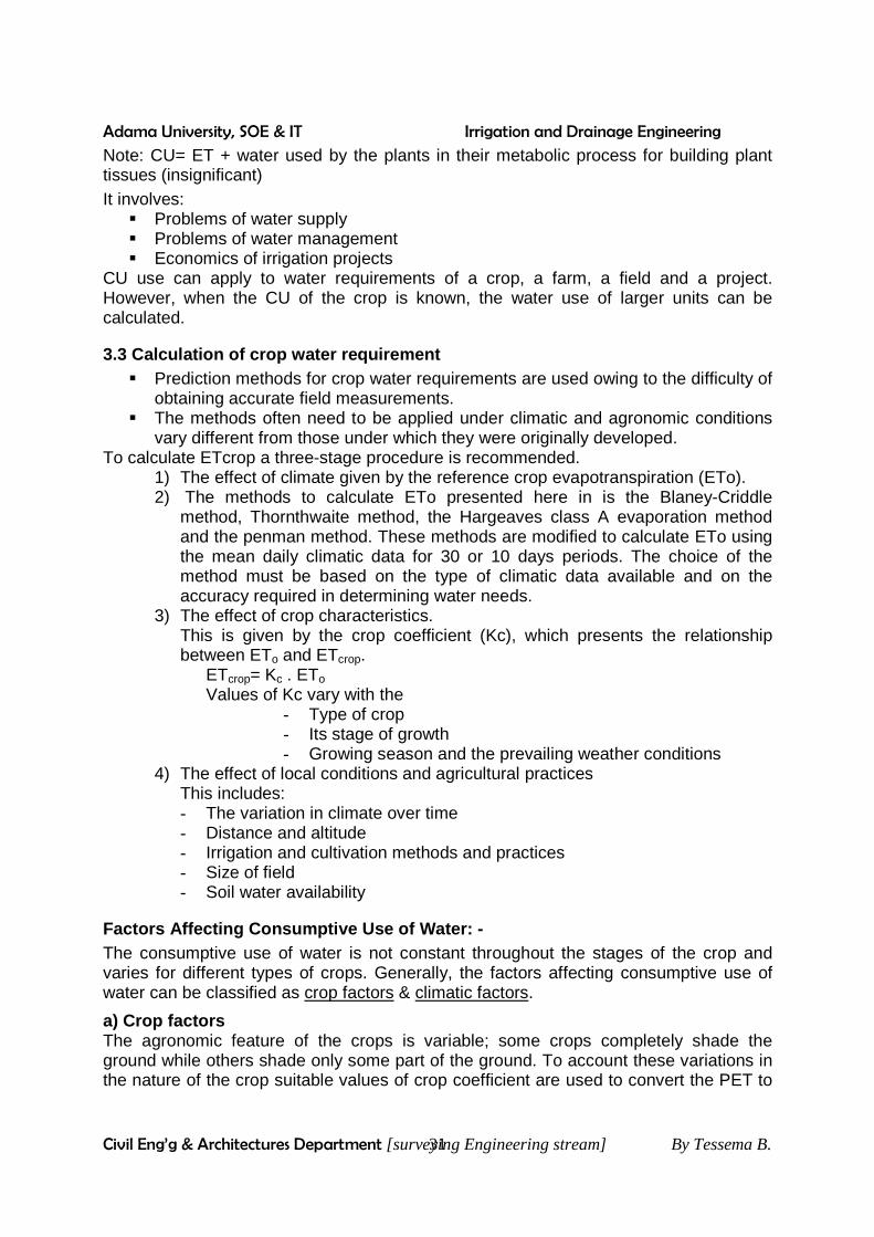
3) The effect of crop characteristics. This is given by the crop coefficient (Kc), which presents the relationship between ETo and ETcrop.
ETcrop= Kc . ETo Values of Kc vary with the
- Type of crop - Its stage of growth - Growing season and the prevailing weather conditions
4) The effect of local conditions and agricultural practices This includes: - The variation in climate over time - Distance and altitude - Irrigation and cultivation methods and practices - Size of field - Soil water availability
Factors Affecting Consumptive Use of Water: - The consumptive use of water is not constant throughout the stages of the crop and varies for different types of crops. Generally, the factors affecting consumptive use of water can be classified as crop factors & climatic factors.
a) Crop factors The agronomic feature of the crops is variable; some crops completely shade the ground while others shade only some part of the ground. To account these variations in the nature of the crop suitable values of crop coefficient are used to convert the PET to

Adama University, SOE & IT Irrigation and Drainage Engineering
Civil Eng’g & Architectures Department [surveying Engineering stream] By Tessema B. 32
actual evapotranspiration. So for the same climatic conditions different crops have different rates of consumptive uses.
b) Climatic factors: Temperature : As the temperature increases, the saturation vapour pressure also increases and results in increase of evaporation and thus consumptive use of water. Wind Speed : The more the speed of wind, the more will be the rate of evaporation; because the saturated film of air containing, the water will be removed easily. Humidity : - The more the air humidity, the less will be the rate of consumptive use of water. This is because water vapour moves from the point of high moisture content to the point of low moisture content. Therefore, if the humidity is high water vapour cannot be removed easily. Sunshine hours : - The longer the duration of the sunshine hour the larger will be the total amount of energy received from the sun. This increases the rate of evaporation and thus the rate of consumptive use of crops.
3.4 Determination of Consumptive Use of water Under normal field, conditions PET (ETO) will not occur and thus consumptive use (ETcrop) can be determined by determining the ETo and multiplying with suitable crop coefficients (Kc). Alternatively, it can be determined by direct measurements of soil moisture. 1) Direct Measurement of Consumptive Use :
A) Lysimeter experiment B) Field experimental plots C) Soil moisture studies D) Water balance method
a) Lysimeter Experiment Lysimeters are large containers having pervious bottom. This experiment involves growing crops in lysimeters there by measuring the water added to it and the water loss (water draining) through the pervious bottom. Consumptive use is determined by subtracting the water draining through the bottom from the total amount of water needed to maintain proper growth. b) Field Experimental Plots: This is most suitable for determination of seasonal water requirements. Water is added to selected field plots, yield obtained from different fields are plotted against the total amount of water used. The yield increases as the water used increases for some limit and then decreases with further increase in water. The break in the curve indicates the amount of consumptive use of water. c) Soil Moisture Studies: In this method soil, moisture measurements are done before and after each irrigation application. Knowing the time gap b/n the two consecutive irrigations, the quantity of water extracted per day can be computed by dividing the total moisture depletion b/n the two successive irrigations by the interval of irrigation. Then a curve is drawn by plotting the rate of use of water against the time from this curve, seasonal water use of crops is determined.
Adama University, SOE & IT Irrigation and Drainage Engineering
Civil Eng’g & Architectures Department [surveying Engineering stream] By Tessema B. 33
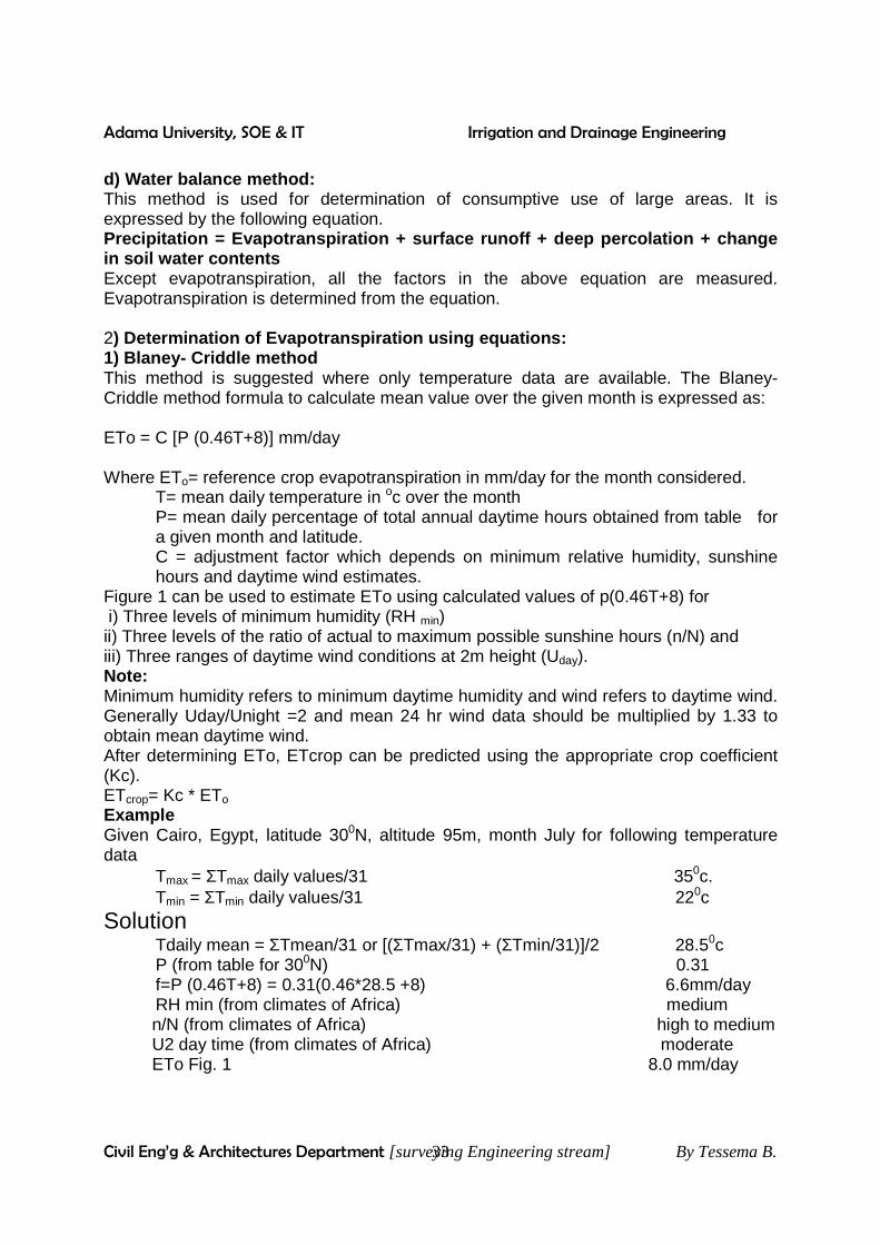
d) Water balance method: This method is used for determination of consumptive use of large areas. It is expressed by the following equation. Precipitation = Evapotranspiration + surface runoff + deep percolation + change in soil water contents Except evapotranspiration, all the factors in the above equation are measured. Evapotranspiration is determined from the equation. 2) Determination of Evapotranspiration using equatio ns: 1) Blaney- Criddle method This method is suggested where only temperature data are available. The Blaney- Criddle method formula to calculate mean value over the given month is expressed as: ETo = C [P (0.46T+8)] mm/day Where ETo= reference crop evapotranspiration in mm/day for the month considered. T= mean daily temperature in oc over the month P= mean daily percentage of total annual daytime hours obtained from table for
a given month and latitude. C = adjustment factor which depends on minimum relative humidity, sunshine
hours and daytime wind estimates. Figure 1 can be used to estimate ETo using calculated values of p(0.46T+8) for i) Three levels of minimum humidity (RH min) ii) Three levels of the ratio of actual to maximum possible sunshine hours (n/N) and iii) Three ranges of daytime wind conditions at 2m height (Uday). Note: Minimum humidity refers to minimum daytime humidity and wind refers to daytime wind. Generally Uday/Unight =2 and mean 24 hr wind data should be multiplied by 1.33 to obtain mean daytime wind. After determining ETo, ETcrop can be predicted using the appropriate crop coefficient (Kc). ETcrop= Kc * ETo Example Given Cairo, Egypt, latitude 300N, altitude 95m, month July for following temperature data Tmax = ΣTmax daily values/31 350c. Tmin = ΣTmin daily values/31 220c
Solution Tdaily mean = ΣTmean/31 or [(ΣTmax/31) + (ΣTmin/31)]/2 28.50c P (from table for 300N) 0.31 f=P (0.46T+8) = 0.31(0.46*28.5 +8) 6.6mm/day RH min (from climates of Africa) medium n/N (from climates of Africa) high to medium U2 day time (from climates of Africa) moderate ETo Fig. 1 8.0 mm/day
Adama University, SOE & IT Irrigation and Drainage Engineering
Civil Eng’g & Architectures Department [surveying Engineering stream] By Tessema B. 34
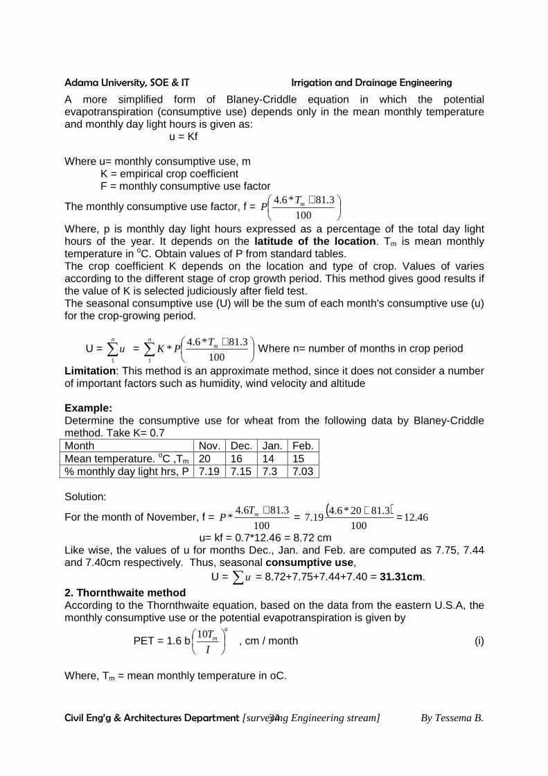
A more simplified form of Blaney-Criddle equation in which the potential evapotranspiration (consumptive use) depends only in the mean monthly temperature and monthly day light hours is given as: u = Kf Where u= monthly consumptive use, m K = empirical crop coefficient F = monthly consumptive use factor
The monthly consumptive use factor, f =
+100
3.81*6.4 mTP
Where, p is monthly day light hours expressed as a percentage of the total day light hours of the year. It depends on the latitude of the location . Tm is mean monthly temperature in oC. Obtain values of P from standard tables. The crop coefficient K depends on the location and type of crop. Values of varies according to the different stage of crop growth period. This method gives good results if the value of K is selected judiciously after field test. The seasonal consumptive use (U) will be the sum of each month's consumptive use (u) for the crop-growing period.
U = ∑n
u1
= ∑
+nmT
PK1 100
3.81*6.4* Where n= number of months in crop period
Limitation : This method is an approximate method, since it does not consider a number of important factors such as humidity, wind velocity and altitude Example: Determine the consumptive use for wheat from the following data by Blaney-Criddle method. Take K= 0.7 Month Nov. Dec. Jan. Feb. Mean temperature. oC ,Tm 20 16 14 15 % monthly day light hrs, P 7.19 7.15 7.3 7.03 Solution:
For the month of November, f = 100
3.816.4*
+mTP =
( )46.12
100
3.8120*6.419.7 =+
u= kf = 0.7*12.46 = 8.72 cm Like wise, the values of u for months Dec., Jan. and Feb. are computed as 7.75, 7.44 and 7.40cm respectively. Thus, seasonal consumptive use , U = ∑u = 8.72+7.75+7.44+7.40 = 31.31cm .
2. Thornthwaite method According to the Thornthwaite equation, based on the data from the eastern U.S.A, the monthly consumptive use or the potential evapotranspiration is given by
PET = 1.6 ba
m
I
T
10 , cm / month (i)
Where, Tm = mean monthly temperature in oC.

Adama University, SOE & IT Irrigation and Drainage Engineering
Civil Eng’g & Architectures Department [surveying Engineering stream] By Tessema B. 35
I = annual heat index, obtained from monthly heat index I of the year
i = 514.1
5
mT and I = ∑
=
12
1n
i = 514.112
1 5∑
=
n
mT (ii)
The values of the exponents a and b are obtained from the relation a = (67.5*10-8) I3 - (77.1*10-6)*I2 + (0.01791) I + 0.492 (iii) b = maximum number of sun shine hrs in the month (IV) 12*30 Example: Estimate the potential evapotranspiration for a crop for the month of June using the Thornthwaite equation from the following data. Month Apr. may June July Aug. Sep. Oct. Temp. T m (oC) 4.5 12.5 20.4 20.2 21.5 10.5 5.5 Max. sun shine hrs 370 380 365 358 355 350 345 Solution: Step 1. Obtain the monthly heat index, i Step 2. Calculate the annual heat index, I Step 3. Determine the constants a & b and finally estimate PET for each month. The monthly heat index is determined as:
i = 514.1
5
mT
Month Apr. May June July Aug. Sep. Oct. Heat index i Factor b
0.85 1.03
4.00 1.06
8.40 1.01
8.28 0.99
9.10 0.99
3.07 0.97
1.16 0.96
Now I = ∑ i = 0.85+4.00+8.4 +8.28+9.10+3.07+1.16 = 34.86
In addition, from equation (iii) a = 1.051 From equation (iv) b = 1.01 Then potential evapotranspiration for the month June is given by:
PET = 1.6 ba
m
I
T
10 = 1.6*1.01* cm35.10
86.34
4.20*10051.1
=
3. Hargreaves class A pan Evaporation ET or CU is related to pan evaporation (EP) by a constant Kc, called consumptive use coefficient.
ET = Kc * Ep Determination of Ep
(a.)Experimentally (b.)Christiansen formula
Ep = 0.459R * Ct*Cw*Ch*Cs*Ce Ct = Coefficient for temperature Ct = 0.393 +0.02796Tc+0.0001189Tc2, Tc= mean temperature, 0c Cw = Coefficient for wind velocity

Adama University, SOE & IT Irrigation and Drainage Engineering
Civil Eng’g & Architectures Department [surveying Engineering stream] By Tessema B. 36
Cw= 0.708+0.0034v-0.0000038v2, v=mean wind velocity at 0.5m above the ground, km/day Ch= Coefficient for relative humidity. Ch= 1.250-0.0087H-0.75*10-4H2 –0.85*10-8H4, H= mean percentage relative humidity at noon Cs= Coefficient for percent of possible sunshine Cs= 0.542+0.008S-0.78*10-4S2+0.62*10-6S3, S= mean sunshine percentage Ce= Coefficient of elevation Ce= 0.97+ 0.00984E, E= elevation in 100 of meters.
4. Modified Penman Method For areas where measured data on temperature, humidity, wind and sunshine duration or radiation are available, the penman method is suggested. The penman equation consists of two terms:
- The energy (radiation) term and - The aerodynamic (wind and humidity) term
The relative importance of each term varies with climatic conditions. Under calm weather conditions, the aerodynamic term is usually less important than the energy term. It is more important under windy conditions and particularly in the more arid regions. A slightly modified penman equation from the original (1948) is suggested here to determine ETo involving a revised wind function term. The method uses mean daily climatic data, since day and night time weather conditions considerably affect level of ET; an adjustment for this is included. The modified penman equation is, ETo = c (W*Rn + (1 – W) * f (u). (ea – ed))
Radiation term Aerody namic term
Where: ETo = reference crop evapotranspiration, mm/day W = temperature related weighting factor Rn = net radiation in equivalent evaporation in, mm/day F (u) = Wind related function (ea-ed)=difference between the saturation vapor pressure at mean air temperature
and the mean actual vapor pressure of the air in mbar. C = adjustment factor to compensate for the effect of day and night weather
condition Due to the interdependence of the variables composing the equation, the correct use of units in which variables need to be expressed is important (see example below).
Description of variables and their Method of calcul ation a) Vapor pressure (e a-ed) Air humidity affects ETo, Humidity is expressed here as saturation vapor pressure deficit (ea-ed),

Adama University, SOE & IT Irrigation and Drainage Engineering
Civil Eng’g & Architectures Department [surveying Engineering stream] By Tessema B. 37
(ea-ed) is the difference between mean saturation water vapor pressure (ea) and the mean actual vapor pressure (ed). Air humidity data are reported as:
- Relative humidity (RH max ad RH min in percentage) - Psychometric readings (T oC of dry and wet bulb) from wet and dry bulb
thermometers, or as a dew point temperature j (Tdew point 0C) Time of measurement is important, but is often not given. Fortunately, actual vapor pressure (ed) is a constant element and even one measurement per day may suffice. Vapor pressure must be expressed in mbar. If ed is given in mm Hg, multiply by 1.33 to find mbar. Tables 5 and 6 give values of ea and ed from available climatic data. Example: Altitude is 0 m. Given : T max 350c, T min 22oc , RHmax 80%, RHmin 30% Calculation T mean = 28.5 oC RHmean = 55% ea at 28.5o
c (Table 5) = 38.9 m bar ed = ea * RHmean/100 = 21.4 m bar (ea-ed) = 17.5 m bar In many regions RH during the night is near 100%, Hence Tmin = Twetbulb
= Tdawpoint, and ed can then be determined from ea at Tmin. b) Wind function (f (u)) The effect of wind on ETo has been studied for different climates resulting in a revised wind function and is given as:
f (u) = 0.27
+100
1U
Where, U is 24 – hr wind run in km /day at 2 m height (Table 7). Where wind data are not collected at 2 m height, the appropriate corrections for wind measurements taken at different heights are given below: Height (m) 0.5 1.0 1.5 2.0 3.0 4.0 5.0 6.0 Correction factor (E) 1.35 1.15 1.06 1.00 0.93 0.88 0.85 0.83

Adama University, SOE & IT Irrigation and Drainage Engineering
Civil Eng’g & Architectures Department [surveying Engineering stream] By Tessema B. 38
Example Given the wind, speed at 3 m height is 250 km/day; calculate the wind function f (U) by applying the correction factor for the wind speed.
Calculation U (applying correction) = 0.93* 250= 23 = 232 km/day f (u) = 0.90 ( from table 7 )
OR f (u) = 0.27*
+100
1 2U
C) Weighting factor (1-w)
(1-w) is a weighting factor for the effect of wind and humidity on ETo
W = / ( +γ)
Where = the rate of change of the saturation vapor pressure with temperature, and γ = the psychometric constant. Values of (1-w) as related to temperature and altitude are given in Table 8. Example: Given the Altitude 95 m, Tmax =35o
C, Tmin = 22oC
Calculation Tmea = 28.5o
C (1-w) (Table 8) = 0.23
D) Weighting factor (W) W is the weighting factor for the effect of radiation of ETo values of W as related to temperature and altitudes are given in Table 9. For temperature use (Tmax + Tmin)/2.
Example Given altitude= 95 m, Tmax= 35 oC, Tmin =22oC, determine the weighting factor W
Calculation Tmean = 28.50
C W (Table 9) = 0.77 E) Net radiation (Rn) Net radiation (Rn) is the difference between all incoming and out going radiation. It can be measured, but such data are rarely available. On the other hand, Rn can be calculated from solar radiation or sunshine hours (or degree of cloud cover), temperature and humidity data. The amount of radiation received at the top of the atmosphere (Ra) is dependent on
- latitude and - time of the year only (Table 10)
Part of Ra is absorbed and scattered when passing through the atmosphere the remainder, including some that is scattered but reaches the earth’s surface is called the solar radiation (Rs). Rs is dependent on Ra and the transmission through the atmosphere that is dependent on cloud cover.
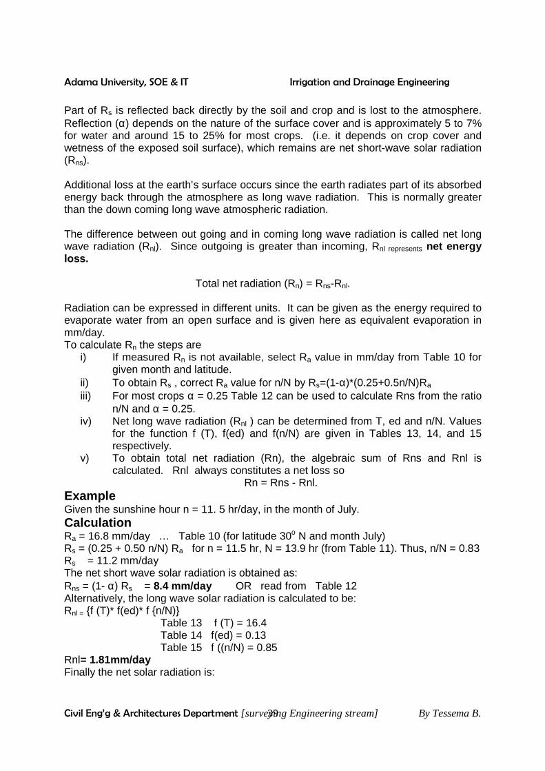
Adama University, SOE & IT Irrigation and Drainage Engineering
Civil Eng’g & Architectures Department [surveying Engineering stream] By Tessema B. 39
Part of Rs is reflected back directly by the soil and crop and is lost to the atmosphere. Reflection (α) depends on the nature of the surface cover and is approximately 5 to 7% for water and around 15 to 25% for most crops. (i.e. it depends on crop cover and wetness of the exposed soil surface), which remains are net short-wave solar radiation (Rns). Additional loss at the earth’s surface occurs since the earth radiates part of its absorbed energy back through the atmosphere as long wave radiation. This is normally greater than the down coming long wave atmospheric radiation. The difference between out going and in coming long wave radiation is called net long wave radiation (Rnl). Since outgoing is greater than incoming, Rnl represents net energy loss.
Total net radiation (Rn) = Rns-Rnl. Radiation can be expressed in different units. It can be given as the energy required to evaporate water from an open surface and is given here as equivalent evaporation in mm/day. To calculate Rn the steps are
i) If measured Rn is not available, select Ra value in mm/day from Table 10 for given month and latitude.
ii) To obtain Rs , correct Ra value for n/N by Rs=(1-α)*(0.25+0.5n/N)Ra iii) For most crops α = 0.25 Table 12 can be used to calculate Rns from the ratio
n/N and α = 0.25. iv) Net long wave radiation (Rnl ) can be determined from T, ed and n/N. Values
for the function f (T), f(ed) and f(n/N) are given in Tables 13, 14, and 15 respectively.
v) To obtain total net radiation (Rn), the algebraic sum of Rns and Rnl is calculated. Rnl always constitutes a net loss so
Rn = Rns - Rnl. Example Given the sunshine hour n = 11. 5 hr/day, in the month of July. Calculation Ra = 16.8 mm/day … Table 10 (for latitude 30o N and month July) Rs = (0.25 + 0.50 n/N) Ra for n = 11.5 hr, N = 13.9 hr (from Table 11). Thus, n/N = 0.83 Rs = 11.2 mm/day The net short wave solar radiation is obtained as: Rns = (1- α) Rs = 8.4 mm/day OR read from Table 12 Alternatively, the long wave solar radiation is calculated to be: Rnl = {f (T)* f(ed)* f {n/N)} Table 13 f (T) = 16.4 Table 14 f(ed) = 0.13 Table 15 f ((n/N) = 0.85 Rnl= 1.81mm/day Finally the net solar radiation is:
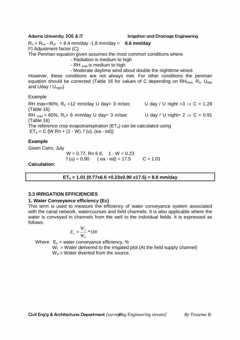
Adama University, SOE & IT Irrigation and Drainage Engineering
Civil Eng’g & Architectures Department [surveying Engineering stream] By Tessema B. 40
Rn = Rns - Rnl = 8.4 mm/day -1.8 mm/day = 6.6 mm/day F) Adjustment factor (C) The Penman equation given assumes the most common conditions where - Radiation is medium to high - RH max is medium to high - Moderate daytime wind about double the nighttime wined. However, these conditions are not always met. For other conditions the penman equation should be corrected (Table 16 for values of C depending on RHmax, Rs, Uday and Uday / Unight)
Example
RH max=90%, Rs =12 mm/day U day= 3 m/sec U day / U night =3 ⇒ C = 1.28 (Table 16) RH max = 60%, Rs= 6 mm/day U day= 3 m/sec U day / U night= 2 ⇒ C = 0.91 (Table 16) The reference crop evapotranspiration (ETo) can be calculated using ETo = C {W.Rn + (1 - W). f (u), (ea - ed)}
Example Given Cairo, July W = 0.77, Rn 6.6, 1 - W = 0.23 f (u) = 0.90 ( ea - ed) = 17.5 C = 1.01 Calculation:
ETo = 1.01 (0.77x6.6 +0.23x0.90 x17.5) = 8.8 mm/day
3.3 IRRIGATION EFFICIENCIES 1. Water Conveyance efficiency (Ec) This term is used to measure the efficiency of water conveyance system associated with the canal network, watercourses and field channels. It is also applicable where the water is conveyed in channels from the well to the individual fields. It is expressed as follows:
100*d
fc W
WE =
Where Ec = water conveyance efficiency, % Wf = Water delivered to the irrigated plot (At the field supply channel) Wd = Water diverted from the source.

Adama University, SOE & IT Irrigation and Drainage Engineering
Civil Eng’g & Architectures Department [surveying Engineering stream] By Tessema B. 41
2. Water application Efficiency (Ea)
After the water reaches the field supply Channel, it is important to apply the water as efficiently as possible. A measure of how efficiently this is done is the water application efficiency.
100*f
sa W
WE =
Where Ea = application efficiency, % Ws = water stored in the rot zone of the plants. Wf = Water delivered to the irrigated plot (At the field supply channel)
Water application efficiency below 100 percent are due to seepage looses from the field distribution channels, deep percolation below the crop root zone and runoff loses from the tail end of borders and furrows ( in very long fields).
3. Water storage efficiency (Es) Small irrigation may lead to high water application efficiencies, yet the irrigation practice may be poor. The concept of water storage efficiency is useful in evaluating this problem. This concept relates how completely the water needed prior to irrigation has been stored in the root zone during irrigation.
100*n
ss W
WE =
Where, Es = Water storage efficiency, % Ws= water stored in the rot zone of the plants. Wn = Water needed in the root zone prior to irrigation Water storage efficiency becomes important when water supplies are limited or when excessive time is required to secure adequate penetration of water in to the soil. In addition, when salt problems exist, the water storage efficiency should be kept high to maintain favorable salt balance. 4. Field Canal Efficiency (E b) This ratio between water received at the field inlet and that received at the inlet of the block of fields.
f
pb W
WE = *100, where Ef = Field canal efficiency
Wp = water received at the field inlet Wf = water delivered to the field channel 5. Water Distribution Efficiency (E d) This shows how uniformly water is applied to the field along the irrigation run. In sandy soils there is generally over irrigation at upper reaches of the run where as in clayey soils, there is over- irrigation at the lower reaches of the run.
1001 xd
yEd
−= Where, Ed = water distribution efficiency, %
d = average depth of water penetration.

Adama University, SOE & IT Irrigation and Drainage Engineering
Civil Eng’g & Architectures Department [surveying Engineering stream] By Tessema B. 42
y = average deviation from d. 6. Water Use Efficiency
This shows the yield of the crop per unit volume of water used. It may be expressed in Kg/ha.cm or q/ha.cm
A. Crop Water Use Efficiency : is the ratio of the crop yield (Y) to the amount of water consumptively used by the crop.
CU
YEw =
B. Field Water Use Efficiency : is the ratio of the crop yield (y) to the total water requirement of crops including Cu losses and other needs.
WR
YEt =
7. Project Efficiency (Ep)
This shows how efficiently the water source used in crop production. It shows the percentage of the total water that is stored in the soil and available for consumptive requirements of the crop. It indicates the overall efficiency of the systems from the headwork to the final use by plants for Cu. The Overall project efficiency must be considered in order to fix the amount of water required at the Diversion headwork. Example: A stream size of 150 lit /sec was released from the diversion headwork to irrigate a land of area 1.8 hectares. The stream size when measured at the delivery to the field channels is 120lit/sec. The stream continued for h hours. The effective root zone depth is 1.80m. The application losses in the field are estimated to be 440m3. The depth of water penetration was 1.80m and 1.20m at the head and tail of the run respectively. The available water holding capacity of the soil is 21cm/m and irrigation was done at 60% depletion of Am. Find Ec, Ef, Ea, Es and Ed. The stream size delivered to the plot was 100 lit/sec. Solution
0%3.83100sec/120
sec/100100
%80100sec/150
sec/120100
===
===
xlit
litx
Wf
WpEf
xlit
litx
Wd
WfEc
Water delivered to the plot = 32880
1000
86060100m
xxx =
Water stored in the root zone =2880m3 – Application losses = 2880m3 - 440m3 = 2440m3

Adama University, SOE & IT Irrigation and Drainage Engineering
Civil Eng’g & Architectures Department [surveying Engineering stream] By Tessema B. 43
%7.841002880
2440100
3
3
=== xm
mx
Wp
WsEa
Total A.M = 21cm/m x 1.80m = 37.80 cm
RAM = cmcmx 68.2280.37
100
60 =
In volume, RAM =
34 4.4082108.1
100
68.22mxx =
%60%8.594.4082
2440100
3
3
≈===m
mx
Wn
WsEs
Average water penetration md 50.12
20.18.1 =+=
Numerical deviation at upper end =1.80 –1.50=0.30m At lower end = 1.50 – 1.20 =0.30m
Average numerical deviation = mx
30,02
30,02
xd
yxEd 1001100 =
− %8050.1
30,01 =
−
3.4 IRRIGATION SCHEDULING Scheduling of irrigation application is very important for successive plant growth and maturity. Water is not applied randomly at any time and in any quantity. Irrigation scheduling is the schedule in which water is applied to the field in an important aspect of an efficient operation of an irrigation system. The scheduling of irrigation can be field irrigation scheduling and field irrigation supply schedules.
Field irrigation Scheduling is done at field level. The two scheduling parameters of field irrigation scheduling are the depth of irrigation and interval of irrigation. 1) Depth of irrigation (d) This is the depth of irrigation water that is to be applied at one irrigation. It is the depth of water that can be retained in the crop root zone b/n the field capacity and the given depletion of the available moisture content. All the water retained in the soil b/n FC and PWP is not readily available to crops. The readily available moisture is only some percentage of the total available moisture. Thus, depth of irrigation is the readily available portion of the soil moisture. In other words, it is the depth of irrigation water required to replenish the soil moisture to field capacity.
The depth of irrigation (d) is given by: d (net) = As. D (FC – PWP). P, m Where As = Apparent specific gravity of soil D = Effective root zone depth in m FC = water content of soil at F.C

Adama University, SOE & IT Irrigation and Drainage Engineering
Civil Eng’g & Architectures Department [surveying Engineering stream] By Tessema B. 44
PWP = Water content of soil at PWP P = depletion factor Because of application lasses such as deep percolation and runoff losses, the total depth of water to be applied will be greater than the net depth of water. The gross depth of application
a
s
E
PPWPFCDAgrossd
*)(**)(
−=
Where Ea = Field application efficiency and other parameters as defined above 1. Interval of Irrigation (i) The interval of irrigation is the time gap in day's b/n two successive irrigation applications. It depends on the type of the crop, soil type and climate conditions. Thus, interval of irrigation depends on the consumptive use rate of the crop and the amount of readily available moisture in the crop root zone. The consumptive use rate of the crop varies from crop to crop and during different stages of the crop. The RAM moisture also varies from soil to soil depending on soil water constants. The interval (frequency) of irrigation is given by:
i(days) = ( )
( )peakcrop
s
ET
PPWPFCDA .. −, where ETcrop(peak) is the peak rate of crop
evapotranspiration in m/day. For the same crop and soil science, the ETcrop (peak) goes on increasing from the initial stage to the development and mid season stage the interval of irrigation will go on decreasing and increasing during rate season stage. Field Irrigation Supply Schedules (Irrigation Sch eduling in a Command Area ) This is the schedule of water supply to individual fields or command area. This is a schedule of the total volume of water to be applied to the soil during irrigation. It depends on crop and soil characteristics. It is expressed as -
( ) APpwpFcDASEa
tq ..(.10
* −= , m3
Where q= Stream size (application rate) lit/sec t = Application time in sec Ea = Application efficiency As = Apparent specific gravity D = Effective root zone depth, m P = Depletion factor A = Area of the command (field) in ha From the above equation, if either of the application time or the stream size fixed, one of them can be determined. In the above equation, q*t indicates the total volume of water applied to the field during irrigation at the head of the field. However, the total volume of water diverted at the headwork will obviously be greater than this value, because there is loss of water during conveyance and distribution canals. The total volume of water to be diverted is given by

Adama University, SOE & IT Irrigation and Drainage Engineering
Civil Eng’g & Architectures Department [surveying Engineering stream] By Tessema B. 45
Q*t = ( ) ..,..10
ApPwPFCDAEp s − , m3
Where Q = flow rate at the headwork, let/sec. Ep = project efficiency and others as defined above. Example 1 For the data below, determine depth & interval of irrigation during different stages. Depth of the root zone = 1 m, FC = 20 %, PWP = 8 %. Dry density of soil=1.6 gm/cm3 and density of water=1gm/cm3. The rates of consumptive uses during different stages are as follows. A depletion of 50% during initial period, 60 % during development and midseason stage and 70 % during late season stage is allowable. Determine the depth and interval of irrigation during different stages of the crop. The CU during different stages is as follows.
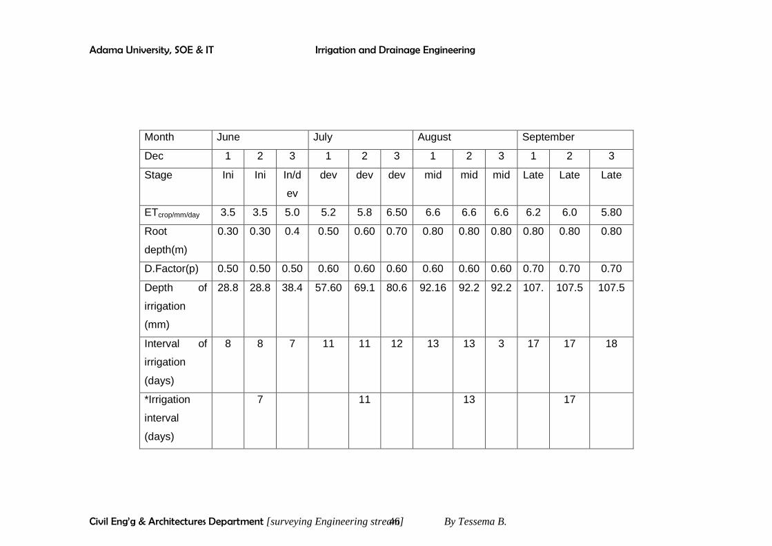
Adama University, SOE & IT Irrigation and Drainage Engineering
Civil Eng’g & Architectures Department [surveying Engineering stream] By Tessema B. 46
Month June July August September
Dec 1 2 3 1 2 3 1 2 3 1 2 3
Stage Ini Ini In/d
ev
dev dev dev mid mid mid Late Late Late
ETcrop/mm/day 3.5 3.5 5.0 5.2 5.8 6.50 6.6 6.6 6.6 6.2 6.0 5.80
Root
depth(m)
0.30 0.30 0.4 0.50 0.60 0.70 0.80 0.80 0.80 0.80 0.80 0.80
D.Factor(p) 0.50 0.50 0.50 0.60 0.60 0.60 0.60 0.60 0.60 0.70 0.70 0.70
Depth of
irrigation
(mm)
28.8 28.8 38.4 57.60 69.1 80.6 92.16 92.2 92.2 107. 107.5 107.5
Interval of
irrigation
(days)
8 8 7 11 11 12 13 13 3 17 17 18
*Irrigation
interval
(days)
7 11 13 17

Adama University, SOE & IT Irrigation and Drainage Engineering
Civil Eng’g & Architectures Department [Surveying Engineering Stream] By Tessema B
47
Example 2
A crop has in effective root zone of 120 cm (1.20 m) prior to irrigation; soil samples were taken from different depths to determine the moisture status of the soil.
Depth of root zone (m) Weight soil sample (gm) Weight of oven dry soil (g)
0 – 0.30 m 0.30 – 0.60 m 0.60 – 0.90 m 0.90 – 1.20 m
98.80 96.60 95.00 94.00
94.60 92.10 90.60 89.40
The water holding capacity of the soil at field capacity is 19.60 cm/meter. The apparent specific gravity of the soil is 1.60. Determine the moisture content in the root zone at different depths total depth of water available in the root zone at different depths, total depth of water available in the root zone and the soil moisture deficit.
Solution
%44.4100*60.94
20.4,
20.460.9480.98
30.00
==
=−=−
gm
gmWcontentMoisture
gmgmgmwaterofMass
mfromdepthFor
In depth of water, d = As. D .p =1.6*0.3*0.0444=0.0213m=2.13cm
For depth 0.3-0.6m: Mass of water=96.60-92.10=4.50gm. W=4.50/92.10 *100= 4.88% In depth, d = As. D.P = 1.60 * 0.30* 0.0488 = 0.0234 = 2.34 cm
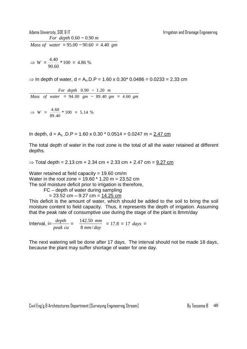
Adama University, SOE & IT Irrigation and Drainage Engineering
Civil Eng’g & Architectures Department [Surveying Engineering Stream] By Tessema B
48
%86.4100*60.90
40.4
40.460.9000.95
90.060.0
==⇒
=−=−
W
gmwaterofMass
mdepthFor
⇒ In depth of water, d = As.D.P = 1.60 x 0.30* 0.0486 = 0.0233 = 2.33 cm
%14.5100*40.89
60.4
60.440.8900.94
20.190.0
==⇒
=−=−
W
gmgmgmwaterofMass
mdepthFor
In depth, d = As .D.P = 1.60 x 0.30 * 0.0514 = 0.0247 m = 2.47 cm The total depth of water in the root zone is the total of all the water retained at different depths. ⇒ Total depth = 2.13 cm + 2.34 cm + 2.33 cm + 2.47 cm = 9.27 cm Water retained at field capacity = 19.60 cm/m Water in the root zone = 19.60 * 1.20 m = 23.52 cm The soil moisture deficit prior to irrigation is therefore, FC – depth of water during sampling
= 23.52 cm – 9.27 cm = 14.25 cm This deficit is the amount of water, which should be added to the soil to bring the soil moisture content to field capacity. Thus, it represents the depth of irrigation. Assuming that the peak rate of consumptive use during the stage of the plant is 8mm/day
Interval, i= daysdaymm
mm
cupeak
depth178.17
/8
50.142 === =
The next watering will be done after 17 days. The interval should not be made 18 days, because the plant may suffer shortage of water for one day.
Adama University, SOE & IT Irrigation and Drainage Engineering
Civil Eng’g & Architectures Department [Surveying Engineering Stream] By Tessema B
49
CHAPTER FOUR
Diversion Head Works
4.1. General
A diversion head works are structures constructed across a river for raising water level in the river so that it can be diverted in to the off taking canals. A diversion head works must be differentiated from storage work or dam. Adam is constructed a cross, a non- perennial or inadequate flow rivers for the purpose of creating a large reservoirs to store water during the period of excess supplies or rains for its use in dry weather flow for meeting the demand. On the other hand, diversion head works are constructed on perennial rivers, which have adequate flow. Therefore, there is no necessity of creating a storage reservoir or very little storage, if any. The diversion head works serves the following purposes:-
i) To raise the water level in the river for increasing its command area ii) To regulate the supply of water in to the canals. iii) To control the silt entry in to the canal iv) To create a small pond (not reservoir) on its upstream and provides some
pond age v) To prevent fluctuations in the level of supply of the river.
4.2 Classification of Diversion Head- works
The diversion head-works may be of temporary or permanent nature depending up on the requirements.
4.2.1. Temporary diversion works (spurs or bunds) These may have temporary boulder walls constructed across a river to raise the level of water and leads it on to a channel. It may be required to construct them every year, as they may be damaged by the floods. 4.2.2 Permanent diversion works (weirs or barrages) 4.2.2.1 Weirs These are solid walls constructed across a river to raise the water level at the up streamside so that the required quantity of water can be diverted in to the canal. It may be provided with small shutters, on its top. During floods as the entire discharge of the river has to pass over the crest, there is considerable afflux on the upstream due to high solid wall.

Adama University, SOE & IT Irrigation and Drainage Engineering
Civil Eng’g & Architectures Department [Surveying Engineering Stream] By Tessema B
50
4.2.2.2 Barrage
The barrage structure is similar to that of the weir but the gate alone affects the heading up of water in the case of a barrage. No solid obstruction is put a cross the river and the crest level in the barrage is kept at low level. During the floods, the gates are raised to clear off the high flood level enabling the high flood to pass down stream with minimum afflux. Again, the gates can be lowered to store water up to the required level.
4.3 Relative advantages and disadvantages of Weirs and Barrages 4.3.1 Weirs Advantages
� The initial cost of weirs is usually low. Disadvantages
� There is a large afflux during floods which causes large submergence � Because the crest is at high level, there is great silting problem. � The raising and lowering of shutters on the crest is not convenient. More over,
it requires considerable time and labor. � The weir lacks an effective control on the river during floods.
4.3.2. Barrages Advantage
� The barrage has a good control on the river during floods. The out flow can be easily regulated by gates
� The afflux during floods is small therefore the submerged area is less � There is a good control over silt entry in to the canal � There is a good control over flow conditions � There are better facilities for inspection & repairs of various structures.
Disadvantage:- The initial cost of the barrage is quite high.
*From the above discussion, a barrage is generally better than a weir. However, they are costlier.
4.4 Ideal Site for diversion Head works An ideal site for diversion head works should have the following characteristics:-
1) The river section at the site should be narrow and well-defined 2) The river should have high; well-defined, ineradicable and non-submersible
banks so that the cost of river training works are minimum 3) The site should be such that the canal commands maximum irrigable areas, with
moderate earth works. 4) There should be suitable arrangement for the diversion of river during
construction 5) The site should be such that the weir (or barrage) can be aligned at right angles
to the direction of the river flow. 6) There should be suitable locations for the under sluices, head regulator and other
components of the diversion head works.

Adama University, SOE & IT Irrigation and Drainage Engineering
Civil Eng’g & Architectures Department [Surveying Engineering Stream] By Tessema B
51
7) The diversion head works should not submerge costly land and property on its upstream.
8) Good foundation should be available at the site 9) The required materials of construction should be available near the site 10) The site should be easily accessible. 11) The overall cost of the project should be minimum
4.4 Types of weirs
A) Classification based on functions i) Storage weirs: - the main function of these weirs is to store water (If the storage
on the u/s of diversion weir is significant). ii) Diversion weirs: - these raise the water level & divert the water to the off taking
canals. iii) Pick-up weirs: - these are diversion headwork constructed on the d/s of a dam
for diverting the water released from the u/s dam in to the off taking canals. B) Classification based on design aspects.
i) Gravity weirs: - the uplift pressure caused by the head of the water seeping below the weir is resisted entirely by the weight of the weir.
ii) Non- Gravity weirs:- the weir floor is designed continuous with the divided piers as reinforced structure such that the weight of concrete slab together with the divide piers keep the structure safe against the up lift.
C) Classification based on construction material. I. vertical drop weir ii. Rock fill weir with sloping apron
iii. Concrete weir with sloping glacis. 4.4.1 Vertical drop weir
� It consists of a masonry wall with a vertical or nearly vertical d/s face & horizontal concrete floor.
The u/s and d/s cutoff walls (or piles) are provided up to the scour depth. The weir floor is designed as a gravity section. The section consists of pitching, block protection & concrete floor on the u/s & d/s of the crest wall. 4.4.2 Rocks fill weirs In addition to the main weir wall, there are a number of core walls. The space b/n the core walls is filled with the fragment rocks. Since rock, fill weirs require many rocks
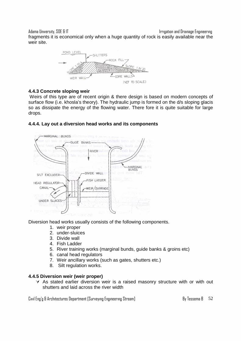
Adama University, SOE & IT Irrigation and Drainage Engineering
Civil Eng’g & Architectures Department [Surveying Engineering Stream] By Tessema B
52
fragments it is economical only when a huge quantity of rock is easily available near the weir site. 4.4.3 Concrete sloping weir Weirs of this type are of recent origin & there design is based on modern concepts of surface flow (i.e. khosla’s theory). The hydraulic jump is formed on the d/s sloping glacis so as dissipate the energy of the flowing water. There fore it is quite suitable for large drops. 4.4.4. Lay out a diversion head works and its compo nents Diversion head works usually consists of the following components.
1. weir proper 2. under-sluices 3. Divide wall 4. Fish Ladder 5. River training works (marginal bunds, guide banks & groins etc) 6. canal head regulators 7. Weir ancillary works (such as gates, shutters etc.) 8. Silt regulation works.
4.4.5 Diversion weir (weir proper)
� As stated earlier diversion weir is a raised masonry structure with or with out shutters and laid across the river width

Adama University, SOE & IT Irrigation and Drainage Engineering
Civil Eng’g & Architectures Department [Surveying Engineering Stream] By Tessema B
53
� The entire length of the weir may be divided in to a number of bays by means of divided piers to avoid cross-flow in floods.
� As far as possible, the weir should be aligned at right angle to the direction of the river flow. This ensures less length of the weir, better discharging capacity & less cost.
4.4.6. Under sluices
� These are gated openings provided in the body of the weir at a lower level
than the crest level of the normal portion of the weir. � If the canal takes off only from one side, the under-sluice section should be
provided near that end only. 4.4.7. Functions of the under sluice i. Help in scouring and removing the deposited silt from the under sluiced pocket and
hence are called the scouring sluices. ii. Enables to admit silt free water in to the canal through head regulator iii. Silt deposited in the u/s side of the weir may be periodically removed over the crest
of the under sluice to the d/s iv. Helps in passing the dry weather flow and low floods v. Creates a clear, unobstructed river channel at the approach portion of the head
regulator vi. Reduce the maximum flood level.
4.4.8 Divide wall � It is a masonry or concrete wall constructed at right angle to the axis of the weir,
and separate the weir proper from the under sluice. � If there are two canals taking off from each flank, then there will be two divided
walls and two under sluices.
4.4.9 Function of the divide wall i. It separate the floor of the scouring sluices from that of the weir proper, which is at a
higher level. ii. It helps in providing a comparatively less turbulent pocket near the canal head
regulator, resulting in depositions of silt in this pocket & thus to help in the entry of silt – free water in to the canal.

Adama University, SOE & IT Irrigation and Drainage Engineering
Civil Eng’g & Architectures Department [Surveying Engineering Stream] By Tessema B
54
iii. It prevents formation of cross currents and the flow parallel to the weir axis, which may cause the formation of vortices and deep scour.
iv. It helps in concentrating the scour action of the under sluices for flushing out the deposited silt in the pocket by ensuring a straight approach to the pocket.
4.4.10. Fish Ladder When a weir is constructed across a river, it forms an obstruction to the free movement of the fishes. To avoid this & to help the survival of the fishes, a fish Ladder is provided. I.e. A fish ladder (fish way) is a passage provided to the divide wall on the weir side for the fish to travel from the u/s to the d/s of the weir and vice verse.
River training works (guide banks, marginal bunds spurs or groins)
� River training works are required near the weir site in order to ensure a smooth and axial flow of water and thus to prevent the river from out flanking the works due to the changes in its course.
4.4.11. Canal head Regulators.
� It is provided at the head of each main canal off taking from the diversion head works.
� In order to reduce silt entry in to the canal the head regulator is usually aligned to make 90 to 1200 from the weir axis.
4.4.12. Function of canal head regulator
i. It regulates the supply of water entering the canal ii. It controls the entry of silt in to the canal. iii. It prevents the river flood from entering the canal.

Adama University, SOE & IT Irrigation and Drainage Engineering
Civil Eng’g & Architectures Department [Surveying Engineering Stream] By Tessema B
55
4.4.13. Weir Design Data
1. The Design Discharge
While designing a weir, provision must be made for the flood that is likely to occur during the lifetime of the structure. Design discharge is the value of the instantaneous peak discharge adopted for the design of a particular project or any other structures.
In addition to the considerations of the flood characteristics, frequencies and potentialities of the contributing drainage area above the structure, socio economic & other non-hydrological considerations, which are likely to have influence, are considered in deriving the design flood.
2. Methods of estimation
� Empirical formula � by physical indication of past flood (flood marks) � Frequency analysis � By unit hydrograph method.
I. Empirical Formula In this method, area of the basin or catchments is considered mainly. All other factors, which influence peak flow, are merged in to constant. A general equation may be written in the form nCAQ = where Q is the peak flow, c is constant, A is area of the catchments has & n is index.
� The constant for a catchment’s is arrived at, after taking the following factors in to account
a. Basin characteristics i). Area ii). Shape iii). Slope b. Storm characteristics i.) Intensity ii). Duration iii). Distribution.
Limitations i. This method does not take frequency of flood in to account. ii. This method cannot be applied universally. iii. Fixing of the constants is very difficult & exact theory cannot be put forth for its
selection. iv. However, they give accurate idea about the peak flow for the catchment’s they
represent.
II. The Slope-Area Method
Design engineers often find themselves in situations where there is no hydrometer in the catchments & if there is, the data series is not complete or its accuracy is doubtful. In these cases, the peak is estimated from the high flood mark on the riverbank & trees.

Adama University, SOE & IT Irrigation and Drainage Engineering
Civil Eng’g & Architectures Department [Surveying Engineering Stream] By Tessema B
56
Old persons in the villages situated on the bank of the river may be contacted to know the maximum water level attained in the past 35 years. The x-section of the river may be plotted and the water line corresponding to the highest flood can be drawn on it. From such x-section, the water flow area, wetted perimeter and hydraulic mean depth can be calculated. By longitudinal sectioning with the help of leveling slightly to the u/s and the d/s of the site where x-section has been plotted, the longitudinal slope of the bed of the river can be determined and the maximum flood discharge can be computed by the manning formula. This procedure should be repeated at several villages or water marks to get consistent results. III, Flood Frequency analysis
Since the exact sequence of stream flow for future years cannot be predicted, probability concepts must be used to study the probable variations in flow so that the design can be completed based on a calculated risk.
To find any design flood of desired frequency a plot of Q versus Tr (recurrence interval) is prepared on probability paper. From this plot, unknown flood for any value of Tr can be found out.
Gumbel’s method, log person distribution & others give a direct formula for obtaining values of flood discharges for recurrence interval. IV. Unit hydrograph method (synthetic unit hydrogra ph) 2. Rating curve
To determine the tail water depth, the rating curve at the location of the weir needs to be known. The curve is usually constructed from the river stage & discharge measurement records. Usually, this data is not available at the location of the weir, there for a theoretical rating curve should be constructed. The following steps can be followed to draw theoretical rating curve:- i. Surveys should be carried out at the location of the weir to draw the x-section of the
river. ii. X- Section to be drawn to a suitable scale. Assume d/t water depths in the river, and
determine the water area & wetted perimeter corresponding to each depth. iii. For each depth, determine the flow velocity and discharges by using the manning
formula. iv. Plot the assumed depths and their corresponding discharges to present the rating
curve. This rating curve is used to determine the water depth corresponding to the river peak flood, which is known as tail water depth.
3. Silt data along with discharge measurements the amount of silt carried by the river is also measured.

Adama University, SOE & IT Irrigation and Drainage Engineering
Civil Eng’g & Architectures Department [Surveying Engineering Stream] By Tessema B
57
The lacey silt factor (f) for the silt at the river site is generally determined from the average size of the particles as f= 1.76 mr where mr is the average size of particle in mm. 4. Full supply level and full supply discharge in the off-taking canal. 5. x- section of the river: - it is very essential to get full information about the x- section
of the river at the weir site u/s & d/s of the site. 6. High flood level & bed level of the river. 7. Amount of afflux or the heading up of water due to the obstruction caused by the
body wall of the weir. 8. Water way or clear space available for the flow of the water. It will be equal to the
length of the weir. The length of the water way for alluvial rivers is usually determined from the lacey wetted perimeter (p) given by p=4.75 Q
4.4.14 Location of the weir Initially it is difficult to decide on the location of the proposed structure with out having topographic maps of the project area and layout of the river course. However, by walking along the river up and d/s of the location where the existing intake is or where the farmers believe it is an appropriate location; it is possible to identify a few places for the proposed structure. The engineer, at this stage, considers the following factors in selecting the structure site.
� Stable bank � Straight portion � No sediment accumulation � Narrow portion � Location of agricultural area � Foundation condition at reasonable depth � Availability of construction material � Response of the local people � Accessibility.
i. Location of the irrigated area If the weir site is too far away from the irrigation area, it means a long main canal is required & hence the need for a high, capital investment. On the other hand, if the site is too close to the proposed land, some of the area in the upper reach of the main canal cannot be commanded.
ii. Stability of the riverbank
Riverbanks are usually unstable in shallow reaches where its cross-section is wide. This implies that a larger & costlier structure is needed in this site than when it is built on a narrow & a more stable section. The location of the weir is chosen where the river is straight, has stable banks and no deposits islands are found iii . Availability of construction materials
When a small-scale structure is to be built, usually the best structure is the one, which uses local materials & expertise. An important factor to be considered is the availability of the proposed construction materials in the area & in the country.

Adama University, SOE & IT Irrigation and Drainage Engineering
Civil Eng’g & Architectures Department [Surveying Engineering Stream] By Tessema B
58
It is absurd to recommend a structure from a material, which has to be imported & involves a waiting period of months or even years. It is advisable, when one deals with a small structure not to take all the decisions purely on the economic basis, but also the psychological effect of implementation delay of the scheme of the farmers.
ii. Availability of satisfactory foundations at reasonable depth. iii. Availability of sufficient labor for construction. iv. Response of people to wards the implementation of the scheme.
4.5 General Design consideration of the weir 1. Crest elevation
The crest elevation of the weir affects the water profile in two ways:-
1. The height of the crest affects the discharge coefficient and consequently the water head above the weir & the backwater curve.
2. The height of the weir affects the shape and location of the jump and the design of the basin.
To full-fill the requirement of the channel intake, the following points should be considered in deciding the level of the crest.
i. The crest level should be so set that the water head required to deliver the main canal
design discharge is obtained ii. The maximum (allowable) u/s water surface elevation must also be considered in
selecting the crest elevation. The maximum allowable water level depends on the u/s riverbank elevation.
2. Length of the weir
Generally, the crest length should be taken as the average wetted width during the flood. In taking the average, the u/s & d/s of the proposed location should be examined & the width at a stable location is measured.
3. Afflux
When the weir obstructs the flow of water in the river, the water will head up on the u/s side of the weir. This rise is maximum during floods. The amount by which the level rises above the normal level is known as afflux. The amount of afflux determines the height and the section of the guide banks & protection bunds used for training the river. Afflux of 1.5 m to 1.0m is commonly provided. 4. Pond level
This is the minimum water level required in the under sluice pocket u/s of the canal head regulator to feed the canal with its full supply. The pond level is generally fixed 1-1.2m above the main canal F.S..L. If the crest level is below the pond level the required pond level should be attained by provision of shutters or gates over the crest.
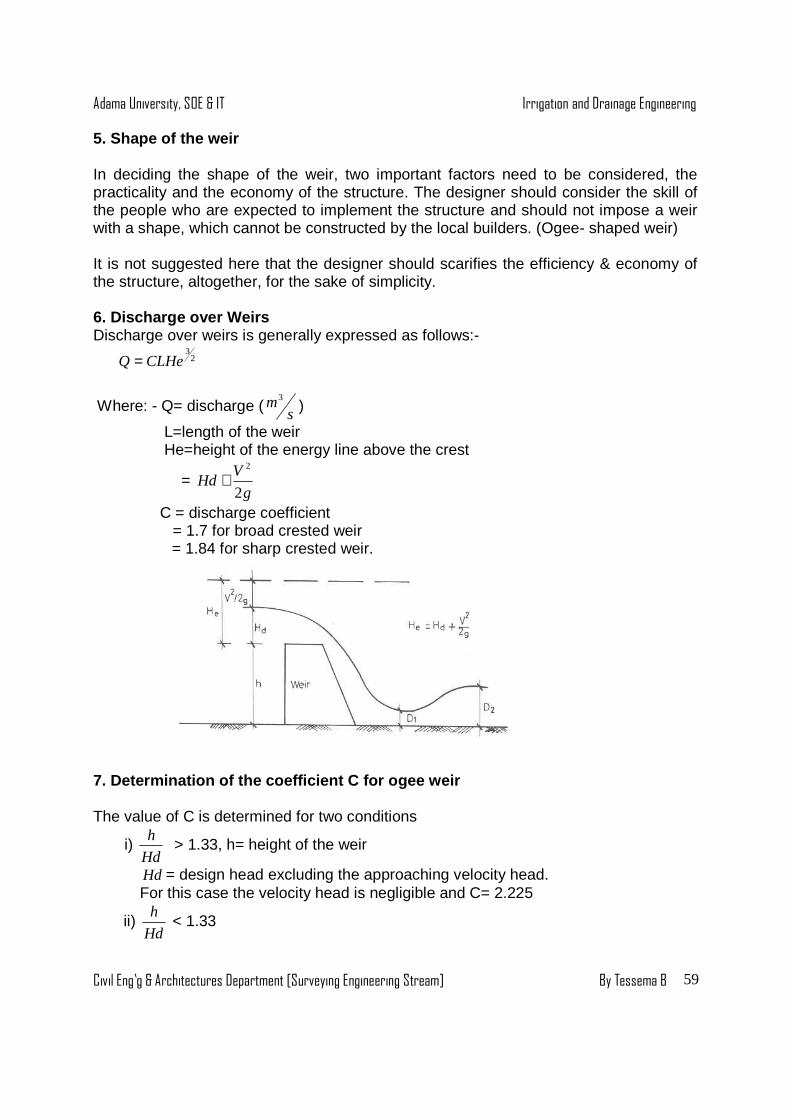
Adama University, SOE & IT Irrigation and Drainage Engineering
Civil Eng’g & Architectures Department [Surveying Engineering Stream] By Tessema B
59
5. Shape of the weir
In deciding the shape of the weir, two important factors need to be considered, the practicality and the economy of the structure. The designer should consider the skill of the people who are expected to implement the structure and should not impose a weir with a shape, which cannot be constructed by the local builders. (Ogee- shaped weir)
It is not suggested here that the designer should scarifies the efficiency & economy of the structure, altogether, for the sake of simplicity.
6. Discharge over Weirs Discharge over weirs is generally expressed as follows:-
23
CLHeQ =
Where: - Q= discharge ( sm3
)
L=length of the weir He=height of the energy line above the crest
= g
VHd
2
2
+
C = discharge coefficient = 1.7 for broad crested weir = 1.84 for sharp crested weir.
7. Determination of the coefficient C for ogee weir
The value of C is determined for two conditions
i) Hd
h > 1.33, h= height of the weir
Hd = design head excluding the approaching velocity head. For this case the velocity head is negligible and C= 2.225
ii) Hd
h < 1.33
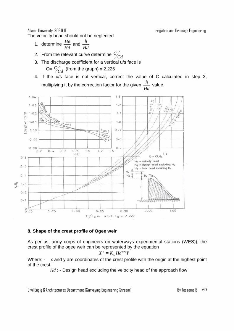
Adama University, SOE & IT Irrigation and Drainage Engineering
Civil Eng’g & Architectures Department [Surveying Engineering Stream] By Tessema B
60
The velocity head should not be neglected.
1. determine Hd
He and
Hd
h
2. From the relevant curve determine CdC
3. The discharge coefficient for a vertical u/s face is
C= CdC (from the graph) x 2.225
4. If the u/s face is not vertical, correct the value of C calculated in step 3,
multiplying it by the correction factor for the given Hd
h value.
8. Shape of the crest profile of Ogee weir
As per us, army corps of engineers on waterways experimental stations (WES)), the crest profile of the ogee weir can be represented by the equation YHdKX n
On 1−=
Where: - x and y are coordinates of the crest profile with the origin at the highest point of the crest. Hd : - Design head excluding the velocity head of the approach flow

Adama University, SOE & IT Irrigation and Drainage Engineering
Civil Eng’g & Architectures Department [Surveying Engineering Stream] By Tessema B
61
oK &n are parameters depending on the slope of the u/s face.
Slope of u/s face Ko n
Vertical 3 on 1 (V:H) 3 on 2 (V.H) 3 on 3
2.00 1.936 1.939 1.873
1.850 1.836 1.810 1.776
4.6. Failure of weir on permeable foundations
Hydraulic structures such as dams, weirs, barrages, head regulators, cross-drainage works, etc. may be founded either on an impervious solid rock foundation or on a pervious foundation. Whenever such structure is founded on a pervious foundation, it is subjected to seepage of water beneath the structure, in addition to all other forces to which it will be subjected when founded on an impervious rock foundation. The water seeping below the body of the hydraulic structure, endangers the stability of the structure and may cause failure by piping or by direct up lift.
i) Failure by piping or undermining : - when the seepage water retains sufficient residual force at the emerging d/s end of the work, it may lift up the soil particles.

Adama University, SOE & IT Irrigation and Drainage Engineering
Civil Eng’g & Architectures Department [Surveying Engineering Stream] By Tessema B
62
This leads to increased porosity of the soil by progressive removal of soil from beneath the foundation. The structure may ultimately subside in to the hollow so formed, resulting in the failure of the structure.
ii) Failure by Direct uplift : - The water seeping below the structure exerts an uplift
pressure on the floor of the structure. If this pressure is not counterbalanced by the weight of the concrete or masonry floor, the structure will fail by rupture of the floor.
4.6.1. Design of weir on permeable Foundation The basic principles for the design of weir on pervious foundations are as follows:-
A) Subsurface Flow
i) The structure should be designed such that the piping failure does not occur due
to subsurface flow ii) The thickness of the floor should be sufficient to resist the uplift pressure due to
sub surface flow. iii) A suitably graded Filter should be provided at the d/s end of the impervious floor
to prevent piping. The filter layer should be loaded with concrete block. iv) D/s pile must be provided to reduce the exit gradient & to prevent piping.
B) Surface Flow i. The piles (or cutoff walls) must be provided up to the maximum scour level at the
ends of the u/s & d/s impervious floor to protect the main structure against scour. ii. Launching aprons should be provided at the u/s and d/s ends to provide a cover to
the main structure against scour. iii. A device is required at the d/s to dissipate energy (due to hydraulic jump) iv. Additional thickness of the impervious floor is provided at the point where the
hydraulic jump is formed to counter balance the suction pressure.
4.7. Sub surface Flow 4.7.1 Methods of seepage Analysis (Theories of sub surface flow )
1. Bligh’s creep Theory As per Bligh, water percolates in to the foundation and creeps or travels slowly through the joint b/n the profile of the weir and the subsoil below it. Further, Bligh assumption is that the subsoil hydraulic gradient, which is the loss of head per unit length of creep, is constant through out the seepage paths & the head lost by the creeping water is proportional to the distance it travels along the base profile of the weir apron.
NB. I) Creep length is the sum of the horizontal & vertical distances traveled by water
through the foundation soil. ii) Hydraulic gradient line: - is an imaginary line joining the water level at the u/s &
d/s side.
Adama University, SOE & IT Irrigation and Drainage Engineering
Civil Eng’g & Architectures Department [Surveying Engineering Stream] By Tessema B
63
Thus according to Bligh theory, the total creep length (L) (Assume negligible floor thickness)
For the case of fig (a) is L=B For the case of Fig (b) is L=B+ 2 (d1+d2+d3)
Bligh called the loss of head per unit length of creep (C= H/L) as percolation coefficient and the reciprocal of percolation coefficient (L/H) as coefficient of creep. He has given the following values of coefficient of creep for d/t soils.
Type of soil Creep coefficient (C=L/H) i) Light sand & mud 18 ii) Fine sand 15 iii) Coarse grained sand 12 iv). Boulder’s & gravel sand mix 5 to 9 Design criteria For design purposes, Bligh gave the following two important criteria. i) Safety Against piping: - the length of creep (L) should be sufficient to provide a safe hydraulic gradient, depending up on the type of soil. Thus safe creep length (L) =CH Where: - L=safe creep length H= Total loss of head of water for the length of creep. C = creep coefficient whose value depends on soil type. ii) Safety Against uplift
The Up lift pressure = v H1
Where: - v= unit weight of water
H1= uplift pressure head at any point of the apron
The down ward force exerted by the material of the Floor = tρv, Where: t= thickness of the apron ρ = specific gravity of floor material Equating up lift pressure with down ward force v H
1= γρt
H1=tρ
'H -t = tρ -t
1
'
−−=
ρtH
t
( )tH −' =h: - ordinate of hydraulic gradient measured above the top of the floor.
)1( −
=ρ
ht
Using factor of safety of 4/3
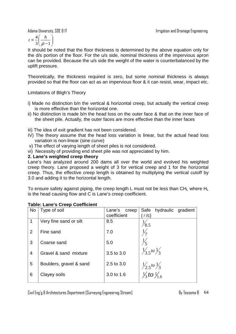
Adama University, SOE & IT Irrigation and Drainage Engineering
Civil Eng’g & Architectures Department [Surveying Engineering Stream] By Tessema B
64
−=
13
4
ρh
t
It should be noted that the floor thickness is determined by the above equation only for the d/s portion of the floor. For the u/s side, nominal thickness of the impervious apron can be provided. Because the u/s side the weight of the water is counterbalanced by the uplift pressure. Theoretically, the thickness required is zero, but some nominal thickness is always provided so that the floor can act as an impervious floor & it can resist, wear, impact etc. Limitations of Bligh’s Theory i) Made no distinction b/n the vertical & horizontal creep, but actually the vertical creep
is more effective than the horizontal one. ii) No distinction is made b/n the head loss on the outer face & that on the inner face of
the sheet pile. Actually, the outer faces are more effective than the inner faces iii) The idea of exit gradient has not been considered. IV) The theory assume that the head loss variation is linear, but the actual head loss
variation is non-linear (sine curve) v) The effect of varying length of sheet piles is not considered. vi) Necessity of providing end sheet pile was not appreciated by him. 2. Lane’s weighted creep theory Lane’s has analyzed around 200 dams all over the world and evolved his weighted creep theory. Lane proposed a weight of 3 for vertical creep and 1 for the horizontal creep. Thus, the effective creep length is obtained by multiplying the vertical cutoff by 3.0 and adding it to the horizontal length. To ensure safety against piping, the creep length L must not be less than CHL where HL is the head causing flow and C is Lane’s creep coefficient. Table: Lane’s Creep Coefficient No Type of soil Lane’s creep
coefficient Safe hydraulic gradient ( l /c)
1 2 3 4 5 6
Very fine sand or silt Fine sand Coarse sand Gravel & sand mixture Boulders, gravel & sand Clayey soils
8.5 7.0 5.0 3.5 to 3.0 2.5 to 3.0 3.0 to 1.6
5.81
71
51
31
5.31 to
31
5.21 to
6.11
31 to

Adama University, SOE & IT Irrigation and Drainage Engineering
Civil Eng’g & Architectures Department [Surveying Engineering Stream] By Tessema B
65
� The weighted creep length should be equal to ( or greater than )the product of the lane’s creep coefficient ( C ) and the seepage head H ( WL CH≥ )
� The thickness of the floor at any point can be determined by computing the uplift pressure head ( h ) & using equation below
−=
13
4
ρh
t
Lane’s weighted creep theory has the same limitations as Bligh’s theory, except the limitation No 1 listed in the preceding section. His theory was an improvement over Bligh’s theory, but however was purely empirical without any rational basis, hence, is generally not adopted in any designs.
3. Khosla’s Theory Weirs designed and constructed by Bligh’s theory have failed due to undermining of subsoil. Dr. Khosla has investigated the problem and draws the following provisional conclusions.
i) The outer faces of the end sheet piles are much more effective than the inner
faces & the horizontal length of the floor. ii) Intermediate piles of smaller in length than the outer plies are in effective,
except for some local redistribution of pressure. iii) Undermining (piping) of the floors starts from the tail end when the hydraulic
gradient at the exit is greater than the critical gradient for that particular soil. (The soil particles move with the flow of water thus causing progressive degradation of the subsoil & resulting in cavities below the floor and ultimately failure.)
iv) It is essential to have a reasonably deep cut off (or pile) at the d/s end of the floor to prevent undermining or piping.
(If a safe value of exit gradient is not obtained, then the depth of cutoff is increased.)
I) Uplift pressure below a horizontal impervious Floor with Intermediate sheet pile.
The uplift pressure at salient points E, D and C are given by the following equation.

Adama University, SOE & IT Irrigation and Drainage Engineering
Civil Eng’g & Architectures Department [Surveying Engineering Stream] By Tessema B
66
PE= )(cos 111
λλ
π−−H
PD = )(cos 11
λλ
π−H
+= −
λλ
π1
cos 11HPC
Where2
11 22
12 ααλ +++=
2
11 22
12
1
ααλ +−+=
d
b11 =α And
d
b22 =α
II. Up lift pressure bellow a horizontal impervious floor with d/s sheet pile.
−= −
λλ
π2
cos 1HPE
−= −
λλ
π1
cos 1HPD
PC=o
Where 2
11 2αλ ++=
In which α=b/d Exit gradient: - the exit gradient (GE) is given by
λπ1
d
HGE =
iii). Up lift pressure below a horizontal impervious floor with u/s sheet pile.
The uplift pressure at the salient points E1, D1 and C1 are given by the following equations. PE1 = H
PD1= )1
(cos 1
λλ
π−−H
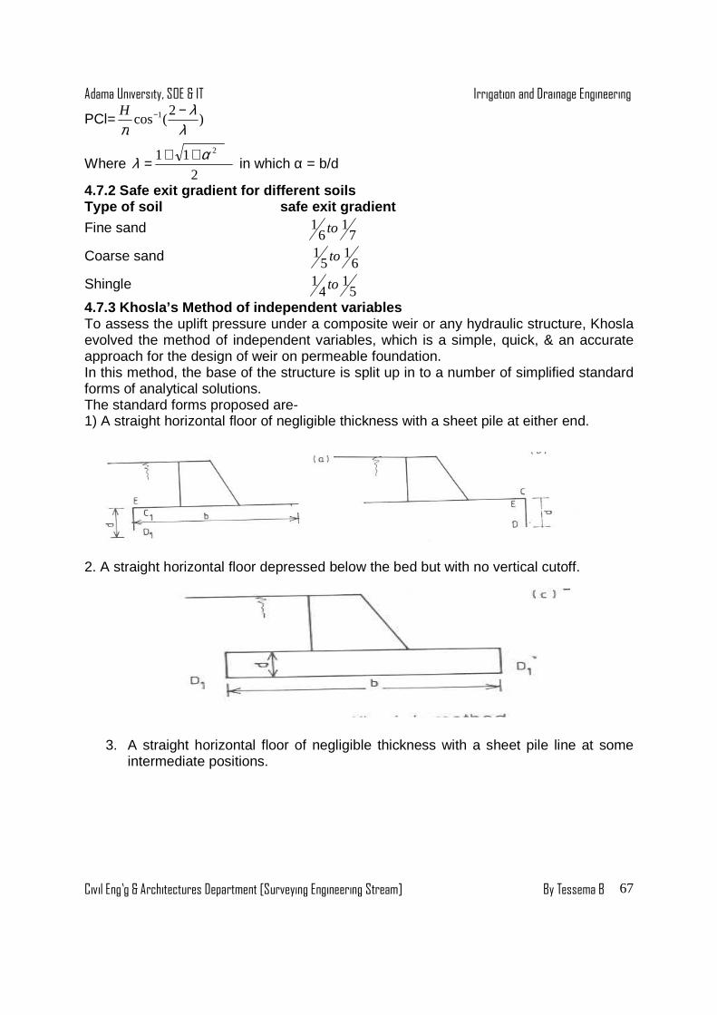
Adama University, SOE & IT Irrigation and Drainage Engineering
Civil Eng’g & Architectures Department [Surveying Engineering Stream] By Tessema B
67
PCl= )2
(cos 1
λλ
π−−H
Where 2
11 2αλ ++= in which α = b/d
4.7.2 Safe exit gradient for different soils Type of soil safe exit gradient
Fine sand 71
61 to
Coarse sand 61
51 to
Shingle 51
41 to
4.7.3 Khosla’s Method of independent variables To assess the uplift pressure under a composite weir or any hydraulic structure, Khosla evolved the method of independent variables, which is a simple, quick, & an accurate approach for the design of weir on permeable foundation. In this method, the base of the structure is split up in to a number of simplified standard forms of analytical solutions. The standard forms proposed are- 1) A straight horizontal floor of negligible thickness with a sheet pile at either end.
2. A straight horizontal floor depressed below the bed but with no vertical cutoff.
3. A straight horizontal floor of negligible thickness with a sheet pile line at some intermediate positions.

Adama University, SOE & IT Irrigation and Drainage Engineering
Civil Eng’g & Architectures Department [Surveying Engineering Stream] By Tessema B
68
The procedure of the analysis consists of i. Splitting up the foundation in to the standard forms ii. Determining the pressure as a percentage of the water head at the key points.
The key points are the junction of the floor and the pile or cutoff walls, the bottom points of the pile or the walls & the bottom corners in the case of depressed floor.
The up lift pressures obtained from the super position of the individual elements are based on the following assumptions
i. The Floor is negligible thickness ii. There is only one pile line iii. The floor is horizontal.
There fore the percentage pressures obtained from the curves of the khosla’s chart of uplift pressures under weir for the simple components of the foundation are valid for the profile as a whole if corrected for:-
a. Mutual interferences of pile b. The floor thickness c. The slope of the floor.
Adama University, SOE & IT Irrigation and Drainage Engineering
Civil Eng’g & Architectures Department [Surveying Engineering Stream] By Tessema B
69
CHAPTER FIVE
DRAINAGE SYSTEM DESIGN 5.1 Drainage of Irrigation Lands 5.1 The need for land drainage Land drainage is the removal of excess surface and sub-surface water from the land to enhance crop growth including the removal of soluble salts. Adverse effects of excess water -Impaired crop growth -Impaired farm operation -the workability of the soil is affected Fewer working days in prolonged periods of excess, water leads to drainage problem Major roles of land drainage
• Prevent the decrease of the productivity of existing cultivated land (it prevents the rise of Water table)
• To control the occurrence of soil salinity • Can hold in the reclamation of already degraded lands (such as waterlogged
areas). Techniques of draining excess water
• Surface drainage • Sub-surface drainage • Improving soil condition through proper management
Knowing the source of excess water leads to find alternative solutions instead of costly drainage system. For instance: If irrigation water is the source of water, then improved irrigation management can avoid excess water. If there is surface inflow from the surrounding hills, then diversions of the inflow water from the area can help. If there is an inflow of ground water to the area, then the construction of tube wells to pump the ground water and discharge it outside the command area can help. If the source of excess water is in the agricultural area, the construction drainage system prevents the excess water. Major Drainage Criteria There are four major drainage criteria 1. Agricultural Drainage Criteria (ADC) It is defined as the criteria specifying the highest permissible levels of the watered table on or in the soil, so that agricultural production is not reduced by problems of water

Adama University, SOE & IT Irrigation and Drainage Engineering
Civil Eng’g & Architectures Department [Surveying Engineering Stream] By Tessema B
70
logging. The design discharge rate is considered. The depth of the water table midway between the drains is decided. The ADC excludes natural drainage system, erosion control, flood protection, and intercepted drainage. 2. Technical Drainage Criteria.
• Due consideration is given to maintain the operation • Depths of the drains, radius of the drainpipes to be used are decided.
3. Environmental Drainage Criteria It is aimed at minimizing the environmental damage due to drainage especially to down stream 4. Economical Drainage Criteria Considers the cost installation and tries to maximize the net benefit 5.2 Surface Drainage Surface drainage is the removal of excess water from the surface (water logging) in time to prevent the land without causing soil erosion. Main components of a drainage system A drainage outlet Main drainage outlet Collector canals (ditches) Fields drains (pipe lines or open channels)
Outlet River Collector Main drainage canal Surface irrigation system is usually applied in relatively flat lands that have soils with low to medium infiltration capacity, low permeability and restricted layer in the soil profile.
Fiels drains

Adama University, SOE & IT Irrigation and Drainage Engineering
Civil Eng’g & Architectures Department [Surveying Engineering Stream] By Tessema B
71
The Agricultural Design Criteria for surface drainage (duration of ponding of water) depends on the sensitivity of the crops to be grown. The negative effects of poor surface drainage system include:
• Inundation of crops resistant to poor growth • Lack of oxygen (leads to poor germination and low nutrient uptake) • Low soil temperature in temperate area
Note : The design of surface drainage system has two components. Land shaping: - shaping of the land surface by land forming (i.e. changing the micro topography). There are two steps during land shaping: i. Land grading –the process of forming the surface to a predetermined grades so that the drainage water easily flow to the drains. It involves cutting and filling ii. Land planning - the process of smoothing the land surface with a land planner to eliminate minor depressions and irregularities without changing the general topography. Construction of open drains to the main outlet. The surface runoff from the fields beds is collected and transported to filed drains and laterals and finally to the outlet. Field Drains
• Are shallow • They usually have “V” shape • Are graded towards the lateral with a maximum grade of 0.1 to 0.3 %
Field Laterals
• Collects water from the field drains and transport it to the main drain • The capacity is larger (multiple of) than field drains • They are constructed by excavation
Design of field drains and laterals 1. Layout: Two types a) Random field drainage system
• Applied when a number of drainage system are distributed at random. b) Parallel field drainage system
• The most effective method of drainage system • It is applied in flat areas.
2. Discharge capacity Open drains should be designed to carry storm runoff, seepage water from subsoil and surface flow due to excess irrigation water applied to the land. The design drainage is usually determined by
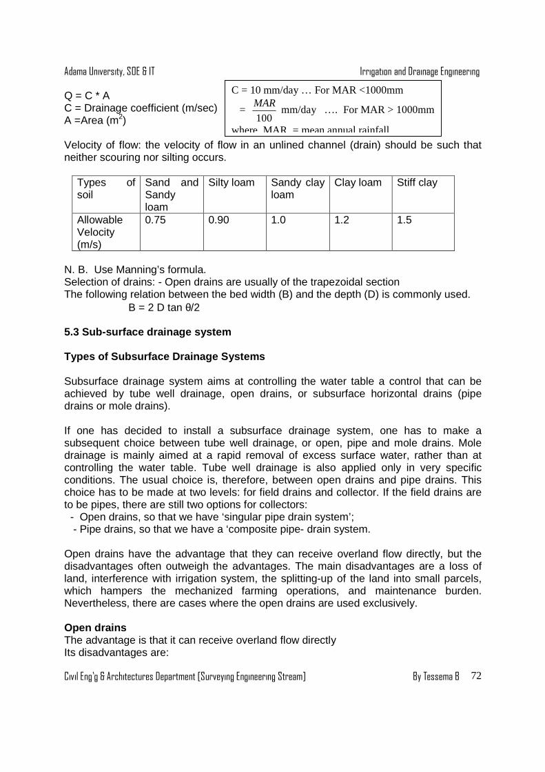
Adama University, SOE & IT Irrigation and Drainage Engineering
Civil Eng’g & Architectures Department [Surveying Engineering Stream] By Tessema B
72
Q = C * A C = Drainage coefficient (m/sec) A =Area (m2) Velocity of flow: the velocity of flow in an unlined channel (drain) should be such that neither scouring nor silting occurs.
Types of soil
Sand and Sandy loam
Silty loam Sandy clay loam
Clay loam Stiff clay
Allowable Velocity (m/s)
0.75 0.90 1.0 1.2 1.5
N. B. Use Manning’s formula. Selection of drains: - Open drains are usually of the trapezoidal section The following relation between the bed width (B) and the depth (D) is commonly used. B = 2 D tan θ/2 5.3 Sub-surface drainage system Types of Subsurface Drainage Systems Subsurface drainage system aims at controlling the water table a control that can be achieved by tube well drainage, open drains, or subsurface horizontal drains (pipe drains or mole drains). If one has decided to install a subsurface drainage system, one has to make a subsequent choice between tube well drainage, or open, pipe and mole drains. Mole drainage is mainly aimed at a rapid removal of excess surface water, rather than at controlling the water table. Tube well drainage is also applied only in very specific conditions. The usual choice is, therefore, between open drains and pipe drains. This choice has to be made at two levels: for field drains and collector. If the field drains are to be pipes, there are still two options for collectors: - Open drains, so that we have ‘singular pipe drain system’; - Pipe drains, so that we have a ‘composite pipe- drain system. Open drains have the advantage that they can receive overland flow directly, but the disadvantages often outweigh the advantages. The main disadvantages are a loss of land, interference with irrigation system, the splitting-up of the land into small parcels, which hampers the mechanized farming operations, and maintenance burden. Nevertheless, there are cases where the open drains are used exclusively. Open drains The advantage is that it can receive overland flow directly Its disadvantages are:
C = 10 mm/day … For MAR <1000mm
= 100
MAR mm/day …. For MAR > 1000mm
where MAR = mean annual rainfall

Adama University, SOE & IT Irrigation and Drainage Engineering
Civil Eng’g & Architectures Department [Surveying Engineering Stream] By Tessema B
73
• Loss of land • Fragmentation of land into parcels • Interference with irrigation system • Maintenance is expensive Pipe drains Types of pipes Pipes envelopes, clay pipes concrete pipes, plastic pipes The criteria for selection depends on the resistance to mechanical and chemical damages 5.4. The design of sub-surface field drainage syste m The design of sub-surface drainage system : - Varies in shape and size that can cover small size or several thousands of ha. It involves the alignment (layout) of the whole drainage system. In values the determination of dimensions, bed slope, water levels (water tables) etc for open drains design and depths & spacing diameter & slopes, elevations of the outlet, etc for pipe drains. 5.4.1 Steady state ground water flow equations These equations are based on the assumptions that the drain discharge equals the recharge to the ground water, and consequently the water table remains in the same position. This is the typical situation in areas with a humid climate and prolonged periods of uniform, medium intensity rainfall. The other assumption is that the rate of recharge to the ground water is uniform and steady and that it equals the discharge through the drainage system. Thus, the water table remains at the same depth as long as the recharge continues. To desirable the flow of ground water to the drains, we have to make the following assumptions: Two-dimensional flow: - This means that the flow is considered identical in any cross-section perpendicular to the drains; which are only true for infinitely long drains. Uniform distribution of recharge Homogeneous and isotropic soils: - We, thus, ignore any spatial variations in the hydraulic conductivity with in the soil layer, although we can treat soil profiles consisting of two or more layers. In drainage studies, we are interested in not only the depth, rise, or fall of Ground water but also on the rate of ground water flow. Application of Darcy’s equation in ground water flow
Q = KA L
Dh

Adama University, SOE & IT Irrigation and Drainage Engineering
Civil Eng’g & Architectures Department [Surveying Engineering Stream] By Tessema B
74
Horizontal flow through layers of soils Assuming that there is no flow across the boundaries, the hydraulic gradient
L
hh
L
h 21 −=∇
The flow rate in each layer of the canal (q, q2 , q3) can be given by
q1 = K1 D1 L
h∇ q2 = K2 D2
L
h∇
q3 = K3 D3 L
h∇
q = q1 + q2 + q3. = L
Dh ( K1D1 + K2 D2 + K3 D3)
KD - transmissivity of the layer Vertical flow through layered soils Assume that not water flows laterally
2
2
32
2
32
2
1
1
21
1
21
1
K
VDhh
D
hhKV
K
VDhh
D
hhKV
=−⇒=
=−⇒−
=
−
( ) ( ) ( )
3
3
2
2
1
1
3
3
2
2
1
1
3
3
2
2
1
1
433231
3
343
3
433
k
D
k
D
k
DDh
VA
Q
k
D
k
D
k
DV
K
VD
K
VD
K
VD
hhhhhhDh
K
VDhh
D
hhKV
++=
++=
++=
−+−+=
=−⇒−=
−
Dupuit-Forcheimer formula
)(2
22
21 hh
L
kq −= This equation is known as Dupuit formula
Where, K = hydraulic conductivity of the soil layer L = drain length

Adama University, SOE & IT Irrigation and Drainage Engineering
Civil Eng’g & Architectures Department [Surveying Engineering Stream] By Tessema B
75
h =head Most drainage equations are based on the Dupuit-Forcheimer assumptions. This is because the Dupuit-Forcheimer assumptions allow us to reduce the three or two-dimensional flow to a one-dimensional flow by assuming parallel and horizontal streamlines. However, such a flow pattern will occur as long as the impervious subsoil is close to the drain. The Hooghoudt equation, which will be described in the following section, is based on these assumptions. If the impervious layer does not coincide with the bottom of the drain, the flow approximately the drains will be radial and the Dupuit-Forcheimers assumptions cannot be applied. Hooghoudt solved this problem also by introducing an imaginary impervious layer to take into account the extra head loss caused by radial flow. The Hooghoudt equation Consider a steady-state flow to vertically walled open drains reaching an impervious layer. According to the Dupuit- Forcheimer theory, Darcy's equation can be applied to describe the flow of ground water (qx) through a vertical plane (y) at distance (x) from the ditch.
dx
dykyqx =
( )
2
2
2
2
48
24
L
khkDhq
L
Dhhkq
+=⇒
+=
If the water level in the drain is very low (D ≈ O) the above equation reduces to
2
24
L
khq =
This equation describes the flow above drain level. If the impervious layer is far below the water level in the drain (D >> h), the second term in the previous equation can be neglected and the equation will reduce to
y
x x
dx
dy
q
Impervious layer
G.S R

Adama University, SOE & IT Irrigation and Drainage Engineering
Civil Eng’g & Architectures Department [Surveying Engineering Stream] By Tessema B
76
2
8
L
Dhkq =
This equation describes the flow below the drain level. These considerations lead to the conclusion that, if the soil profile consists of two layers with different hydraulic conductivities, and if the drain level is at the interface between the soil layers, the equation can be written as
2
248
L
hkDhKq tb +=
Kt = hydraulic conductivity of the layer above drain level Kb = hydraulic conductivity of the layer below drain level. The Ernst Equation So far, we have only discussed solutions that can be applied for a homogeneous soil profile or for a two layered soil profile if the interface between the two layers coincides with the drain level. The Ernst equation is applicable to any type of two-layered soil profile. It has the advantage over the Hooghoudt equation that the interface between the two layers can be either above or below drain level. It is especially useful when the top layer has considerably lower hydraulic conduction than the bottom layer. To obtain generally applicable solution for soil profiles consisting of layers with different hydraulic conductivities Ernest (1956, 1962) divided the flow to the drains into vertical, horizontal and radial components. Consequently, the total available head (h) can be divided in to a head loss caused by the vertical flow (hv), the horizontal flow (hh) and the radial flow (hr) i.e. h = hv + hh + hr Vertical flow Vertical flow is assumed to take place in the layer between the water table and the drain level. We can obtain the head loss caused by the vertical flow by applying Darcy’s low.
vertical
Horizontal Radial
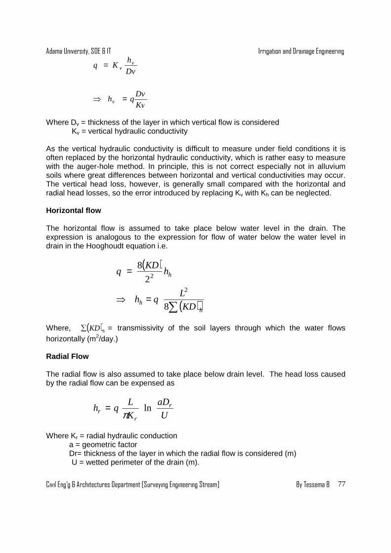
Adama University, SOE & IT Irrigation and Drainage Engineering
Civil Eng’g & Architectures Department [Surveying Engineering Stream] By Tessema B
77
Kv
Dvqh
Dv
hKq
v
vv
=⇒
=
Where Dv = thickness of the layer in which vertical flow is considered Kv = vertical hydraulic conductivity As the vertical hydraulic conductivity is difficult to measure under field conditions it is often replaced by the horizontal hydraulic conductivity, which is rather easy to measure with the auger-hole method. In principle, this is not correct especially not in alluvium soils where great differences between horizontal and vertical conductivities may occur. The vertical head loss, however, is generally small compared with the horizontal and radial head losses, so the error introduced by replacing Kv with Kh can be neglected. Horizontal flow The horizontal flow is assumed to take place below water level in the drain. The expression is analogous to the expression for flow of water below the water level in drain in the Hooghoudt equation i.e.
( )
( )∑=⇒
=
hh
h
KD
Lqh
hKD
q
8
2
8
2
2
Where, ( ) =∑ hKD transmissivity of the soil layers through which the water flows horizontally (m2/day.) Radial Flow The radial flow is also assumed to take place below drain level. The head loss caused by the radial flow can be expensed as
U
aD
K
Lqh r
rr ln
π=
Where Kr = radial hydraulic conduction a = geometric factor Dr= thickness of the layer in which the radial flow is considered (m) U = wetted perimeter of the drain (m).
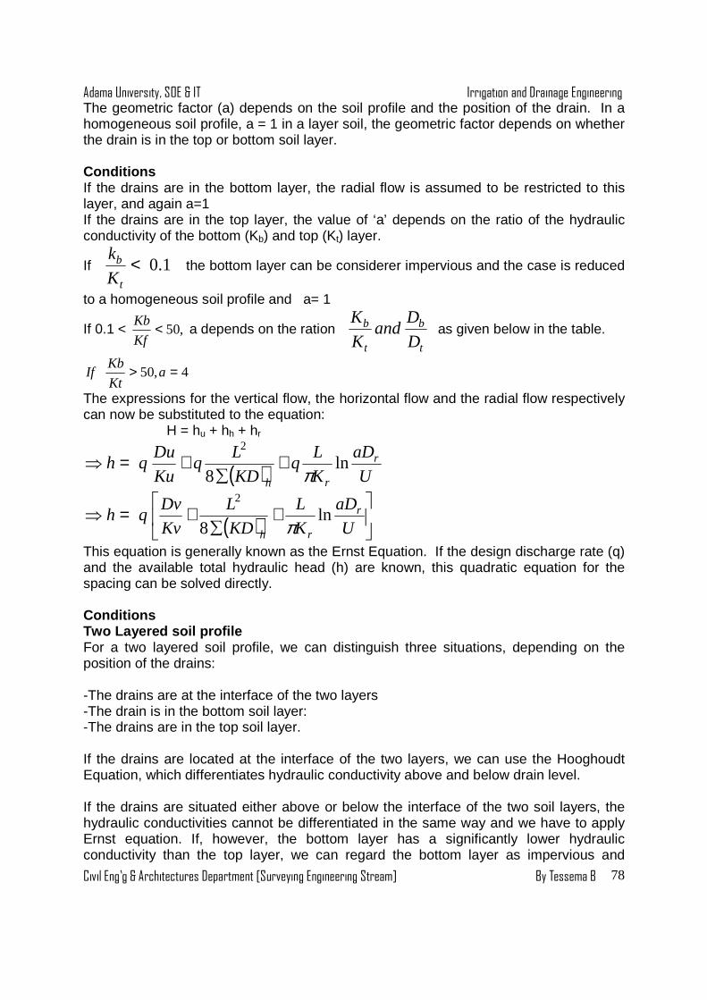
Adama University, SOE & IT Irrigation and Drainage Engineering
Civil Eng’g & Architectures Department [Surveying Engineering Stream] By Tessema B
78
The geometric factor (a) depends on the soil profile and the position of the drain. In a homogeneous soil profile, a = 1 in a layer soil, the geometric factor depends on whether the drain is in the top or bottom soil layer. Conditions If the drains are in the bottom layer, the radial flow is assumed to be restricted to this layer, and again a=1 If the drains are in the top layer, the value of ‘a’ depends on the ratio of the hydraulic conductivity of the bottom (Kb) and top (Kt) layer.
If 1.0<t
b
K
k the bottom layer can be considerer impervious and the case is reduced
to a homogeneous soil profile and a= 1
If 0.1 < ,50<Kf
Kb a depends on the ration
t
b
t
b
D
Dand
K
K as given below in the table.
4,50 => aKt
KbIf
The expressions for the vertical flow, the horizontal flow and the radial flow respectively can now be substituted to the equation: H = hu + hh + hr
( ) U
aD
K
Lq
KD
Lq
Ku
Duqh r
rh
ln8
2
π+
∑+=⇒
( )
+
∑+=⇒
U
aD
K
L
KD
L
Kv
Dvqh r
rh
ln8
2
π
This equation is generally known as the Ernst Equation. If the design discharge rate (q) and the available total hydraulic head (h) are known, this quadratic equation for the spacing can be solved directly. Conditions Two Layered soil profile For a two layered soil profile, we can distinguish three situations, depending on the position of the drains: -The drains are at the interface of the two layers -The drain is in the bottom soil layer: -The drains are in the top soil layer. If the drains are located at the interface of the two layers, we can use the Hooghoudt Equation, which differentiates hydraulic conductivity above and below drain level. If the drains are situated either above or below the interface of the two soil layers, the hydraulic conductivities cannot be differentiated in the same way and we have to apply Ernst equation. If, however, the bottom layer has a significantly lower hydraulic conductivity than the top layer, we can regard the bottom layer as impervious and
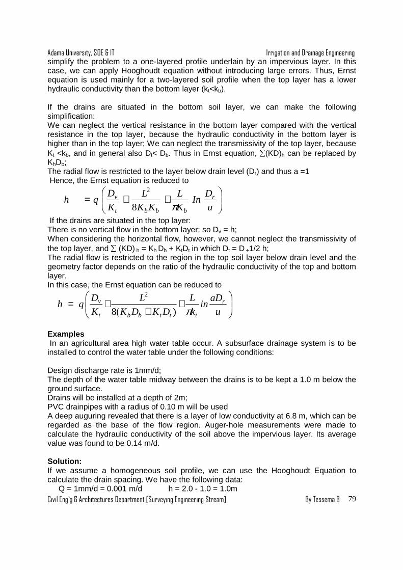
Adama University, SOE & IT Irrigation and Drainage Engineering
Civil Eng’g & Architectures Department [Surveying Engineering Stream] By Tessema B
79
simplify the problem to a one-layered profile underlain by an impervious layer. In this case, we can apply Hooghoudt equation without introducing large errors. Thus, Ernst equation is used mainly for a two-layered soil profile when the top layer has a lower hydraulic conductivity than the bottom layer (kt<kb). If the drains are situated in the bottom soil layer, we can make the following simplification: We can neglect the vertical resistance in the bottom layer compared with the vertical resistance in the top layer, because the hydraulic conductivity in the bottom layer is higher than in the top layer; We can neglect the transmissivity of the top layer, because Kt <kb, and in general also Dt< Db. Thus in Ernst equation, ∑(KD)h can be replaced by KhDb; The radial flow is restricted to the layer below drain level (Dr) and thus a =1 Hence, the Ernst equation is reduced to
++=
u
DIn
K
L
KK
L
K
Dqh r
bbbt
v
π8
2
If the drains are situated in the top layer: There is no vertical flow in the bottom layer; so Dv = h; When considering the horizontal flow, however, we cannot neglect the transmissivity of the top layer, and ∑ (KD) h = Kh Dh + KtDt in which Dt = D +1/2 h; The radial flow is restricted to the region in the top soil layer below drain level and the geometry factor depends on the ratio of the hydraulic conductivity of the top and bottom layer. In this case, the Ernst equation can be reduced to
+
++=
u
aDin
k
L
DKDK
L
K
Dqh r
tttbbt
v
π)(8
2
Examples In an agricultural area high water table occur. A subsurface drainage system is to be installed to control the water table under the following conditions: Design discharge rate is 1mm/d; The depth of the water table midway between the drains is to be kept a 1.0 m below the ground surface. Drains will be installed at a depth of 2m; PVC drainpipes with a radius of 0.10 m will be used A deep auguring revealed that there is a layer of low conductivity at 6.8 m, which can be regarded as the base of the flow region. Auger-hole measurements were made to calculate the hydraulic conductivity of the soil above the impervious layer. Its average value was found to be 0.14 m/d. Solution: If we assume a homogeneous soil profile, we can use the Hooghoudt Equation to calculate the drain spacing. We have the following data: Q = 1mm/d = 0.001 m/d h = 2.0 - 1.0 = 1.0m
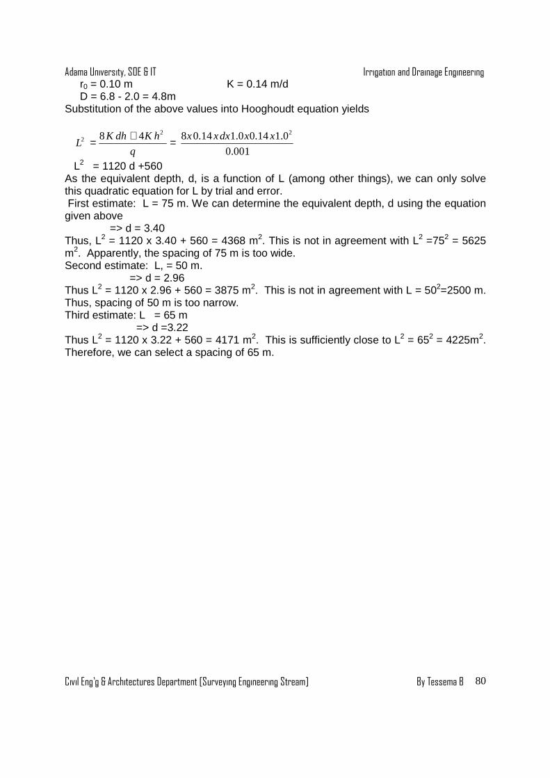
Adama University, SOE & IT Irrigation and Drainage Engineering
Civil Eng’g & Architectures Department [Surveying Engineering Stream] By Tessema B
80
r0 = 0.10 m K = 0.14 m/d D = 6.8 - 2.0 = 4.8m Substitution of the above values into Hooghoudt equation yields
001.0
0.114.00.114.0848 222 xxdxxx
q
hKdhKL =+=
L2 = 1120 d +560 As the equivalent depth, d, is a function of L (among other things), we can only solve this quadratic equation for L by trial and error. First estimate: L = 75 m. We can determine the equivalent depth, d using the equation given above => d = 3.40 Thus, L2 = 1120 x 3.40 + 560 = 4368 m2. This is not in agreement with L2 =752 = 5625 m2. Apparently, the spacing of 75 m is too wide. Second estimate: L, = 50 m. => d = 2.96 Thus L2 = 1120 x 2.96 + 560 = 3875 m2. This is not in agreement with L = 502=2500 m. Thus, spacing of 50 m is too narrow. Third estimate: L = 65 m => d =3.22 Thus L2 = 1120 x 3.22 + 560 = 4171 m2. This is sufficiently close to L2 = 652 = 4225m2. Therefore, we can select a spacing of 65 m.

Adama University, SOE & IT Irrigation and Drainage Engineering
Civil Eng’g & Architectures Department [Surveying Engineering Stream] By Tessema B
81
CHAPTER SIX
IRRIGATION METHODS
6.1 SURFACE IRRIGATION METHODS
6.1.1 General
The term surface irrigation refers to a broad class of irrigation in which the soil surface conveys and distributes water over the irrigated field and at the same time infiltrates into the underlying profile. It is the oldest and still the most widely used method of water application to agricultural land. Irrigation systems generally consist of four components;
1) Physical systems 3) Social and organizational systems 2) Cropping system 4) Economic systems
1. Physical systems The primary purpose of the physical system is to supply water to an area for crop production. The Physical systems of Surface irrigation systems as a whole consist of four subsystems. These are i) Water supply system This includes surface and under ground water sources. ii) Water delivery system The function of water delivery sub- system is to convey water from the source to field through main canal, distributaries, minors and field channels, at constant, regulated rate, at proper elevation, with seepage controlled, with out excessive erosion or sediment taken, with appropriate water quality and . iii) Water Application subsystems The out put from water delivery sub –system is the input for water application Sub-system. Functions:
• To distribute the desired amount of water with the designed uniformity over the field
• To satisfy erosion control standards • To provide necessary surface drainage
Water use subsystem The water use sub- system receives water from the application sub-system. Functions : - • To supply the water requirement of the crop

Adama University, SOE & IT Irrigation and Drainage Engineering
Civil Eng’g & Architectures Department [Surveying Engineering Stream] By Tessema B
82
• To maintain acceptable level of soil salinity • To ensure adequate nutrients • To provide soil conditions for supporting plants, preventing soil crusting facilitating
tillage etc iv) Water removal subsystem This sub –system is used for removal and disposal of surface and sub- surface waters from land to improve agriculture operations. Functions: -
• To provide proper root aeration by lowering ground water table • To maintain appropriate salinity levels with in the soil profile • To dispose (remove) excess irrigation or rainwater from the field
2. Irrigated cropping system An irrigated cropping system is defined as all the elements required for production of a particular crop or set of crops and inter relationships between the crop or set of crops and the environment with this context, cropping system, consists • Plant environment: - crop types grown in the area. • Farm management: - the management practices of the farm and its effect on
irrigated cropping system Important aspects
• Tillage operation • Irrigation practices • Soil fertility management • Seed bed management • Crop management
3. Social and organizational systems
This deals with the interrelationships between social groups and organizations in the development and management of sustainable irrigation system.
4. Economic System This deals with the overall benefits obtained from the system and its accompanying costs incurred.
In this chapter, an attempt is made to discuss only on the water use system.

Adama University, SOE & IT Irrigation and Drainage Engineering
Civil Eng’g & Architectures Department [Surveying Engineering Stream] By Tessema B
83
Figure6.1. The four subsystems of an irrigation system Advantages and disadvantages of surface irrigation Surface irrigation offers a number of advantages at both the farm and project level.
� It is more acceptable to agriculturalists that appreciate the effect of water shortage on crop yield since it appears easier to apply the depth required to fill the root zone
� It can be developed at the farm level with minimal capital investment � The major capital expense of the surface irrigation system is generally
associated with land grading � Energy requirements for surface irrigation systems come from gravity � Surface irrigations are less affected by climatic and water quality characteristics.

Adama University, SOE & IT Irrigation and Drainage Engineering
Civil Eng’g & Architectures Department [Surveying Engineering Stream] By Tessema B
84
� Generally, the gravity flow system is highly flexible, relatively easily managed method of irrigation.
Note There is one disadvantage of surface irrigation tha t confronts every designer and irrigator. � It is very difficult to define the primary design v ariables, discharge and time of application,
due to the highly spatial and temporal variability of the soil.
6.1.2 Surface Irrigation Processes and Methods 6.1.2.1 Surface Irrigation Processes (hydraulic pha ses ) In surface irrigation, water is applied directly to the soil surface from a channel located at the upper reach of the field. Gravity provides the major driving force to spread water over the irrigated field. Once distributed over the surface of the field and after it has entered the soil, water is often redistributed by forces other than gravity. Generally, in a surface irrigation event four distinct hydraulic phases can be discerned: 1. Advance phase : the time interval between the start of irrigation and arrival of the advancing (wetting) front at the lower end of the field.
2. Ponding (wetting storage or continuing) phase : - the irrigation time extending between the end of advance and inflow cutoff. The term “Wetting” phase is usually used for furrow and border where tail water runoff can occur, whereas ponding is the preferred term for basin irrigation (no tail water runoff)
. 3. Depletion (vertical recession) phase : the time interval between supply cut-off and the time that water dries up at the inlet boundary.
4. Recession (horizontal recession) phase : the time required the water to recede from all points in the channel, starting from the end of the depletion phase. The time difference at each measuring station between the clock time or cumulative time for advance and recession is the opportunity time, T, infiltration to occur.

Adama University, SOE & IT Irrigation and Drainage Engineering
Civil Eng’g & Architectures Department [Surveying Engineering Stream] By Tessema B
85
Figure 6.2: Phases of Irrigation systems
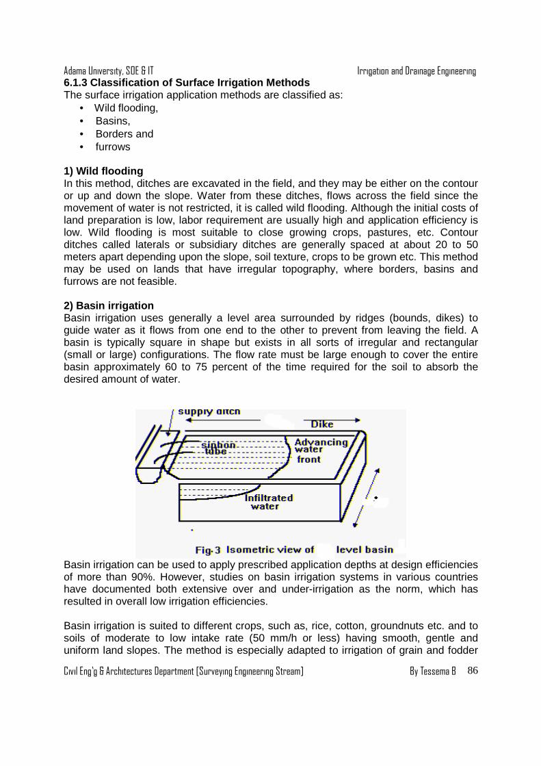
Adama University, SOE & IT Irrigation and Drainage Engineering
Civil Eng’g & Architectures Department [Surveying Engineering Stream] By Tessema B
86
6.1.3 Classification of Surface Irrigation Methods The surface irrigation application methods are classified as:
• Wild flooding, • Basins, • Borders and • furrows
1) Wild flooding In this method, ditches are excavated in the field, and they may be either on the contour or up and down the slope. Water from these ditches, flows across the field since the movement of water is not restricted, it is called wild flooding. Although the initial costs of land preparation is low, labor requirement are usually high and application efficiency is low. Wild flooding is most suitable to close growing crops, pastures, etc. Contour ditches called laterals or subsidiary ditches are generally spaced at about 20 to 50 meters apart depending upon the slope, soil texture, crops to be grown etc. This method may be used on lands that have irregular topography, where borders, basins and furrows are not feasible. 2) Basin irrigation Basin irrigation uses generally a level area surrounded by ridges (bounds, dikes) to guide water as it flows from one end to the other to prevent from leaving the field. A basin is typically square in shape but exists in all sorts of irregular and rectangular (small or large) configurations. The flow rate must be large enough to cover the entire basin approximately 60 to 75 percent of the time required for the soil to absorb the desired amount of water.
Basin irrigation can be used to apply prescribed application depths at design efficiencies of more than 90%. However, studies on basin irrigation systems in various countries have documented both extensive over and under-irrigation as the norm, which has resulted in overall low irrigation efficiencies. Basin irrigation is suited to different crops, such as, rice, cotton, groundnuts etc. and to soils of moderate to low intake rate (50 mm/h or less) having smooth, gentle and uniform land slopes. The method is especially adapted to irrigation of grain and fodder

Adama University, SOE & IT Irrigation and Drainage Engineering
Civil Eng’g & Architectures Department [Surveying Engineering Stream] By Tessema B
87
crops in heavy soils where water is absorbed very slowly and is required to stand for a relatively long time to ensure adequate irrigation. 3) Border irrigation Border irrigation makes use of parallel earth rides to guide a sheet of flowing water across a field. The land between two levees is called a border strip, simply called a border. Border strips, like basins, can be described as rectangular channels (narrow or wide) in which the width of flow plays a dominant role in affecting the geometric elements of the channel. The border strip may vary from 3 to 30 meters in width and from 100 to 800 meters in length. Border irrigation is a more controlled version of wild flooding with additional field ditches that serve as supply sources for applying water to the field.
Figure6.4: Isometric view of border strips
Border irrigation is generally well suited to soils with moderately high intake rates and to slopes less than 0.5 percent. The method can be classified as straight or contour borders depending on weather the borders are running along or across the main slope. Borders can be grouped into three major categories depending on the management strategy adopted:
(1) Fixed flow: - A system in which the inlet flow rate remains constant throughout the duration of irrigation, the method is simple and less expensive but generally of low efficiency.
(2) Cutback : - This is a system in which irrigation begins with a maximum or near maximum non-erosive inlet flow rate, which continues for a part of the irrigation period and then reduced to a level just above what is needed to wet the entire length of the border.
(3) Tail water reuse :- this is a system in which excess surface runoff from the downstream end is collected in a sump and then pumped back into the same field to open up more borders or used to irrigate another field.
Field application efficiency is good to excellent if the border strips are designed and installed properly and good water management practice is followed. Design water application efficiencies of the order 70 -75 % can be attained for slopes of 0.001 to

Adama University, SOE & IT Irrigation and Drainage Engineering
Civil Eng’g & Architectures Department [Surveying Engineering Stream] By Tessema B
88
0.002 m/m on soils of silty clay to clay with depth of application of 75 - 100 mm. For high efficiencies, the stream size and the resulting rate of advance must be controlled to match the recession conditions to provide approximately equal infiltration opportunity time at both the upper and lower ends. 4) Furrow irrigation Furrow irrigation refers to water that is discharged into and runs down small sloping channels (called furrows or corrugations) which are cut or pressed into the soil. The two most common furrow irrigation systems are the straight furrow irrigation and graded furrow irrigation. Water infiltrates from the bottom and sides of furrows moving laterally downward to wet the soil and to move soluble salts, fertilizers and herbicides carried in the water.
When properly designed and operated, furrow irrigation systems may result in a good performance. The wide variations in furrow cross-section types as well as the two dimensional nature of the infiltration process under furrow irrigation complicates mathematical analysis and field measurement needed to quantify irrigation parameters compared to other two methods. Efforts to achieve high application efficiencies for furrow-irrigated systems are limited by very large spatial and temporal variation in infiltration characteristics. Thus, while efficiencies of 85 to 90 % are periodically reported from studies incorporating careful soil moisture monitoring and automation, efficiencies in the order of 50 to 70 % are more common. Moreover, designs could be acceptable if the water application efficiency is greater than 70 percent, with less than 10 percent deep percolation and 20 percent runoff losses, while storage efficiency is greater than 85 to 90 percent. Most crops would be irrigated by the furrow method and is best suited to medium to moderately fine textured soils with relatively high water holding capacity and conductivity, which allow significant water movement in both the horizontal and vertical directions. As border irrigation, furrow irrigation systems, can be grouped into fixed flow,
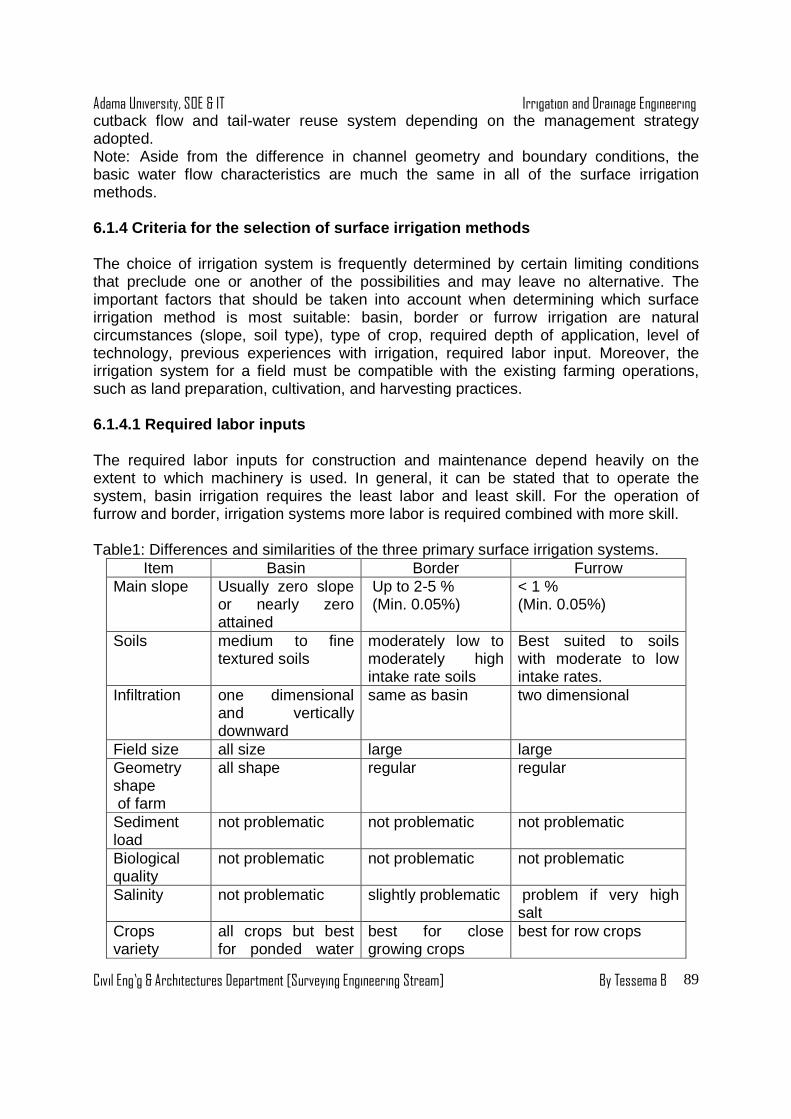
Adama University, SOE & IT Irrigation and Drainage Engineering
Civil Eng’g & Architectures Department [Surveying Engineering Stream] By Tessema B
89
cutback flow and tail-water reuse system depending on the management strategy adopted. Note: Aside from the difference in channel geometry and boundary conditions, the basic water flow characteristics are much the same in all of the surface irrigation methods. 6.1.4 Criteria for the selection of surface irrigat ion methods The choice of irrigation system is frequently determined by certain limiting conditions that preclude one or another of the possibilities and may leave no alternative. The important factors that should be taken into account when determining which surface irrigation method is most suitable: basin, border or furrow irrigation are natural circumstances (slope, soil type), type of crop, required depth of application, level of technology, previous experiences with irrigation, required labor input. Moreover, the irrigation system for a field must be compatible with the existing farming operations, such as land preparation, cultivation, and harvesting practices. 6.1.4.1 Required labor inputs The required labor inputs for construction and maintenance depend heavily on the extent to which machinery is used. In general, it can be stated that to operate the system, basin irrigation requires the least labor and least skill. For the operation of furrow and border, irrigation systems more labor is required combined with more skill. Table1: Differences and similarities of the three primary surface irrigation systems.
Item Basin Border Furrow Main slope Usually zero slope
or nearly zero attained
Up to 2-5 % (Min. 0.05%)
< 1 % (Min. 0.05%)
Soils medium to fine textured soils
moderately low to moderately high intake rate soils
Best suited to soils with moderate to low intake rates.
Infiltration
one dimensional and vertically downward
same as basin two dimensional
Field size all size large large Geometry shape of farm
all shape regular regular
Sediment load
not problematic not problematic not problematic
Biological quality
not problematic not problematic not problematic
Salinity not problematic slightly problematic problem if very high salt
Crops variety
all crops but best for ponded water
best for close growing crops
best for row crops
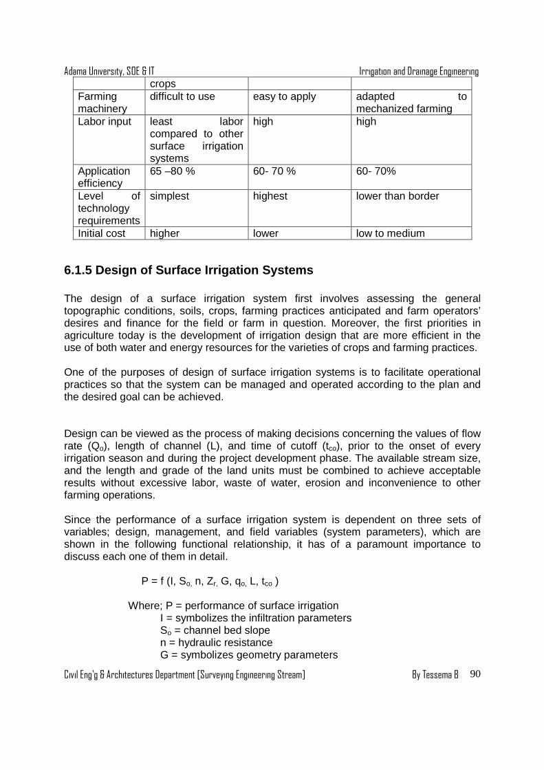
Adama University, SOE & IT Irrigation and Drainage Engineering
Civil Eng’g & Architectures Department [Surveying Engineering Stream] By Tessema B
90
crops Farming machinery
difficult to use easy to apply adapted to mechanized farming
Labor input least labor compared to other surface irrigation systems
high high
Application efficiency
65 –80 % 60- 70 % 60- 70%
Level of technology requirements
simplest highest lower than border
Initial cost higher lower low to medium
6.1.5 Design of Surface Irrigation Systems The design of a surface irrigation system first involves assessing the general topographic conditions, soils, crops, farming practices anticipated and farm operators’ desires and finance for the field or farm in question. Moreover, the first priorities in agriculture today is the development of irrigation design that are more efficient in the use of both water and energy resources for the varieties of crops and farming practices. One of the purposes of design of surface irrigation systems is to facilitate operational practices so that the system can be managed and operated according to the plan and the desired goal can be achieved. Design can be viewed as the process of making decisions concerning the values of flow rate (Qo), length of channel (L), and time of cutoff (tco), prior to the onset of every irrigation season and during the project development phase. The available stream size, and the length and grade of the land units must be combined to achieve acceptable results without excessive labor, waste of water, erosion and inconvenience to other farming operations. Since the performance of a surface irrigation system is dependent on three sets of variables; design, management, and field variables (system parameters), which are shown in the following functional relationship, it has of a paramount importance to discuss each one of them in detail. P = f (I, So, n, Zr, G, qo, L, tco ) Where; P = performance of surface irrigation I = symbolizes the infiltration parameters So = channel bed slope n = hydraulic resistance G = symbolizes geometry parameters

Adama University, SOE & IT Irrigation and Drainage Engineering
Civil Eng’g & Architectures Department [Surveying Engineering Stream] By Tessema B
91
Zr = required amount of application qo = unit flow rate at the head end of the channel tco = time of cut off L = furrow length A) Surface irrigation Design inputs (System Parame ters and System Variables) Generally, there are two types of design data inputs in surface irrigation: field parameters and field decision variables. The designer can manipulate decision variables. They include flow rate, the field dimensions and cut-off time. On the other hand, however, the designer cannot influence Field parameters; they are measured or assumed properties of the given situation. They primarily consist of the soil infiltration characteristics, the flow resistance, the required net application depth, and the field slopes (for borders and furrows). System Parameters 1. Required amount of application (Zr):- This parameter represents the amount of water that needs to be stored in the crop root zone reservoir during every irrigation, in order to sustain normal crop growth. The crop type, stage of growth, presence or absence of shallow water table, and limiting soil horizons (such as hard pans), among other things, determine the effective crop root depth. Soil type is the factor that determines how much water can be stored per unit depth of soil. These factors, along with the climatic conditions of an area should be considered to determine the required amount of application (Zr). For basins and borders the characteristics width is unit width, i.e. 1m, whereas for furrows it is the furrow spacing.
Note: Zr is the same as MAD, and is determined as: Zr = MAD = TAW * f
2. Maximum allowable flow velocity ( Vmax):- This is used in estimating the non-erosive flow rate, Qmax, which can be turned on into a furrow, a border, or a basin without causing soil erosion. The value of Vmax is generally dependent on soil type, and may vary within the range of 8 m/min for erodiable silt to 13 m/min for more stable clay and sandy soils 3. Manning’s roughness coefficient (n):- A parameter in Manning’s equation, known as the Manning’s n, is used as a measure of the resistance effects that flow might encounter as it moves down the furrow, border or basin, which is in fact a representation, in lumped form, of the effect of the roughness of the physical boundaries of the flow and cultivation practices. Most of the time, the values for Manning’s n used for furrow, border and basin irrigation are based on the recommendation of the SCS and are given in the following table. Table2. Commonly used values of Manning’s, n in surface irrigation Field condition Manning’s n values Smooth bare soil surface non-cultivated, oil-mulched citrus 0.04 Small grain, drill rows parallel to direction of irrigation 0.10 Alfalfa, mint, broadcast small grain, and similar crops 0.15 Dense sod crops, small grain with drill rows across the border strip
0.25
Source: USDA, 1979
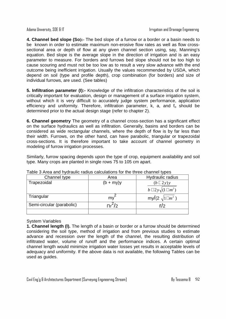
Adama University, SOE & IT Irrigation and Drainage Engineering
Civil Eng’g & Architectures Department [Surveying Engineering Stream] By Tessema B
92
4. Channel bed slope ( So):- The bed slope of a furrow or a border or a basin needs to be known in order to estimate maximum non-erosive flow rates as well as flow cross-sectional area or depth of flow at any given channel section using, say, Manning’s equation. Bed slope is the average slope in the direction of irrigation and is an easy parameter to measure. For borders and furrows bed slope should not be too high to cause scouring and must not be too low as to result a very slow advance with the end outcome being inefficient irrigation. Usually the values recommended by USDA, which depend on soil (type and profile depth), crop combination (for borders) and size of individual furrows, are used. (See tables) 5. Infiltration parameter (I):- Knowledge of the infiltration characteristics of the soil is critically important for evaluation, design or management of a surface irrigation system, without which it is very difficult to accurately judge system performance, application efficiency and uniformity. Therefore, infiltration parameter, k, a, and fo should be determined prior to the actual design stage (refer to chapter 2). 6. Channel geometry The geometry of a channel cross-section has a significant effect on the surface hydraulics as well as infiltration. Generally, basins and borders can be considered as wide rectangular channels, where the depth of flow is by far less than their width. Furrows, on the other hand, can have parabolic, triangular or trapezoidal cross-sections. It is therefore important to take account of channel geometry in modeling of furrow irrigation processes.
Similarly, furrow spacing depends upon the type of crop, equipment availability and soil type. Many crops are planted in single rows 75 to 105 cm apart.
Table 3 Area and hydraulic radius calculations for the three channel types
Channel type Area Hydraulic radius Trapezoidal (b + my)y
)1(2
)2(2myb
yyb
+++
Triangular my2 my/(2 21 m+ )
Semi-circular (parabolic) Πr2/2 r/2
System Variables 1. Channel length (l). The length of a basin or border or a furrow should be determined considering the soil type, method of irrigation and from previous studies to estimate advance and recession over the length of the channel, the resulting distribution of infiltrated water, volume of runoff and the performance indices. A certain optimal channel length would minimize irrigation water losses yet results in acceptable levels of adequacy and uniformity. If the above data is not available, the following Tables can be used as guides.

Adama University, SOE & IT Irrigation and Drainage Engineering
Civil Eng’g & Architectures Department [Surveying Engineering Stream] By Tessema B
93
Table4. Typical border slopes, length and width for different soils
Soil type Slope ranges (%)
Length ranges (M)
Width ranges
(M) Sandy to sandy loams
0.25-0.6 60-120 15-20
Medium loam
0.2-0.4 100-180 20-25
Clay to clay loam
0.05-0.2 150-300 25-35
Table 5 Maximum furrows lengths for given slopes, depth of water application and soils. Furrow Slope
Average depth of water applied (mm) 75 150 225 50 100 150 50 75 100
Clays Loams
Sands Percent Meter 0.1 340 440 470 180 340 440 90 120 190 0.3 400 500 620 280 400 500 150 220 280 0.5 400 500 560 280 370 470 120 190 250 2.0 220 270 340 180 250 300 60 90 150
2. Unit inlet flow rate (Qu):- This is the discharge diverted into a furrow, or a unit width border or a basin. Inlet flow rate is one of the key variables in influencing the outcome of an irrigation event; it affects, the rate of advance to a significant degree and recession to a lesser but appreciable extent thereby having a significant effect on uniformity, efficiency and adequacy of irrigation. It should not be too high as to cause scouring and should not be too small as otherwise the water will not advance to the down stream end.
3. Cutoff time (tco ):- Cutoff time is the time at which the supply is turned off, measured from the onset of irrigation. The ideal time of cutoff occurs when the infiltrated depth in the least-watered portion of the field is equal to the irrigation requirement. The most important effect of cutoff is reflected on the amount of losses, deep percolation and surface runoff, and hence efficiency and adequacy of irrigation. In general, for any given
factor level of combination the selection of an appropriate value of tco is made based on the target application depth and acceptable level of deficit.
B) Surface irrigation system performance Ideally the best surface irrigation scenario (event) is one that can apply the right amount of water over the entire subject area and without loss, a situation which requires that equal amount of water be applied over the entire reach of the channel. However, in practice there exist no surface irrigation system or operation scenarios that can apply water without loss and with perfect uniformity. In any case making uneven application of water over the length of run of a channel is unavoidable. The inevitable consequence of

Adama University, SOE & IT Irrigation and Drainage Engineering
Civil Eng’g & Architectures Department [Surveying Engineering Stream] By Tessema B
94
this is in order to apply a certain target amount of water at a point, down stream end of the subject area; a larger amount must be applied at another point. What all these indicate is that in real life systems uneven and excess application of irrigation water are the “twins facts of lif e’ that engineers and irrigators ought to live with. We cannot do without them but we ought to strive to minimize them. That is what system design and management is all about. The merit of an irrigation scenario (event) is judged in terms of indices that “measure how close an irrigation scenario is to the ideal one”. These indices are collectively referred to as performance indices . The performance of a surface irrigation event can be evaluated from three distinct but complementary perspectives. (1) Excess application of irrigation water : - though unavoidable in real life situation must be minimized (minimum loss). Application efficiency (Ea) is the index, which is used as a measure of how effective irrigation is in minimizing unavoidable losses. (2) Adequacy of irrigation: - evaluated in terms of a perceived requirement is necessary to sustain normal crop growth and result in satisfactory yield. Water storage efficiency (Es) uses how close the applied amount is to the perceived requirement (right amount). (3) Uniform (even) application: - of irrigated water over the entire subject, area not only enhances productive use of available water by spreading deficit, if any, over the subject area but also helps minimize losses. Distribution uniformity (DU) and Christiansen's uniformity coefficient (UC) are the most commonly used indices in surface irrigation application. Moreover, deep percolation and run-off losses are vital in constraining as well as guiding operational decision-making processes. It nonetheless is appropriate to threat them as performance term as per scenario.
Irrigation uniformity Uniformity of infiltration under surface irrigation depends on the spatial and temporal variability of surface and sub-surface hydraulic characteristics such as field slope, furrow geometry, surface roughness, field length, flow rate and soil pore size distribution. Two parameters are used to evaluate distribution uniformity:- • The first parameter is distribution uniformity coefficient DU , and is defined as the
ratio of the minimum infiltrated amount expressed as percentage of the average infiltrated amount over the subject area.
A general expression for DU is - 100*min
avZ
ZDU = .
Where, Zmin = minimum infiltrated amount over the length of the run of the subject area (m3. m-1).
Zav = average infiltrated amount over the length of the run of the subject area (m3. m-1).
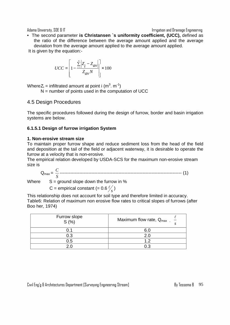
Adama University, SOE & IT Irrigation and Drainage Engineering
Civil Eng’g & Architectures Department [Surveying Engineering Stream] By Tessema B
95
• The second parameter is Christansen `s uniformity coefficient, (UCC), defined as the ratio of the difference between the average amount applied and the average deviation from the average amount applied to the average amount applied.
It is given by the equation:-
UCCZi Zav
Zav Ni
N
= −−∑
×=1 1001
Where Zi = infiltrated amount at point i (m3. m-1) N = number of points used in the computation of UCC 4.5 Design Procedures The specific procedures followed during the design of furrow, border and basin irrigation systems are below.
6.1.5.1 Design of furrow irrigation System 1. Non-erosive stream size To maintain proper furrow shape and reduce sediment loss from the head of the field and deposition at the tail of the field or adjacent waterway, it is desirable to operate the furrow at a velocity that is non-erosive. The empirical relation developed by USDA-SCS for the maximum non-erosive stream size is
Qmax = S
C--------------------------------------------------------------------------------- (1)
Where S = ground slope down the furrow in %
C = empirical constant (= 0.6 sl )
This relationship does not account for soil type and therefore limited in accuracy. Table6: Relation of maximum non erosive flow rates to critical slopes of furrows (after Boo her, 1974)
Furrow slope S (%) Maximum flow rate, Qmax ,
s
l
0.1 6.0 0.3 2.0 0.5 1.2 2.0 0.3

Adama University, SOE & IT Irrigation and Drainage Engineering
Civil Eng’g & Architectures Department [Surveying Engineering Stream] By Tessema B
96
Table7. Intake family and advance coefficients for depth of infiltration in mm, time in minutes and length in meters.
Intake family a b c f g 0.05 0.10 0.15 0.20 0.25 0.30 0.35 0.40 0.45 0.50 0.60 0.70 0.80 0.90 1.00 1.50 2.00
0.5334 0.6198 0.7110 0.7772 0.8534 0.9246 0.9957 1.064 1.130 1.196 1.321 1.443 1.560 1.674 1.786 2.284 2.753
0.618 0.661 0.683 0.699 0.711 0.720 0.729 0.736 0.742 0.748 0.757 0.766 0.773 0.779 0.785 0.799 0.808
7.0 7.0 7.0 7.0 7.0 7.0 7.0 7.0 7.0 7.0 7.0 7.0 7.0 7.0 7.0 7.0 7.0
7.16 7.25 7.34 7.43 7.52 7.61 7.70 7.79 7.88 7.97 8.15 8.33 8.50 8.68 8.86 9.76
10.65
1.088*10-4 1.251*10-4 1.414*10-4 1.578*10-4 1.741*10-4 1.904*10-4 2.067*10-4 2.230*10-4 2.393*10-4 2.556*10-4 2.883*10-4 3.209*10-4 3.535*10-4 3.862*10-4 4.188*10-4 5.819*10-4 7.451*10-4
The average intake over the length of the furrow is given by-
I = LP
1 (Vin - V0ut – Vs) --------------------------------------------------------- (2)
Where i = equivalent depth infiltrated over wetted surface area of field, mm L= distance between inflow and outflow measurements, m P = adjusted wetted perimeter, m V = volume of water (inflow, outflow, storage) in liter
The adjusted wetted perimeter in given by the following equation
P = 0.265 227.0425.0
5.0+
S
Qn -------------------------------------------------- (3)
Where Q= volumetric inflow rate, sl
N =Manning’s roughness coefficient
S = furrow slope or hydraulic gradient, mm
In most cases, after the flow has stabilized and gets uniform, the hydraulic gradient is equal to the furrow slope. A roughness coefficient of 0.04 is normally used for design of furrow irrigation system. The volume of channel storage is given by-
Vs =
−
0217.0947.2
305.0
735.0
5.0S
QnL-------------------------------------------------- (4)

Adama University, SOE & IT Irrigation and Drainage Engineering
Civil Eng’g & Architectures Department [Surveying Engineering Stream] By Tessema B
97
The required depth of infiltration for a furrow system must be expressed as an equivalent depth over the total field area. Infiltration depth is given by:
i = [ ]w
pCat b + ---------------------------------------------------------------------- (5)
Where a, b, c are intake family coefficients t = time, min W = furrow spacing, m p = adjusted wetted perimeter, m
The advance time for stream of water moving down the furrow is given by-
Tt =
5.0
expQS
gx
f
x-------------------------------------------------------------- (6)
Where Tt = advance time, min X = distance down the furrow, m F = advance coefficient (Table 6.6) g= advance coefficient
Q= volumetric inflow rate, sl
S = furrow slope, mm
The infiltration opportunity time is equal to the time of water application minus the advance time plus the recession time. To = Tco – Tt + Tr , min --------------------------------------------- (7) The cut-off time, Tco, reflects an irrigation management decision made by the farmer and designer. It should be an adequate length of time to infiltrate a satisfactory depth of water over the length of the furrow with out causing excessive deep percolation. Tco is normally set equal to the time to advance to the end of the furrow plus the required net infiltration time less recession time. Letting in equal the desired net depth of infiltration, the net infiltration time is determined by
Tn =
b
n
a
Cp
wi
1
−
---------------------------------------------- (8)
The recession time is assumed Zero for open- ended gradient furrows (i.e. for furrows whose slope is not equal to zero) with out loss of accuracy. For gradient furrows, To = Tco – Tt ------------------------------------------------------------------------------------- (9) But Tco = Tt + Tn Where Tt = advance time required to reach end of the field at distance L, min.
Let β = 5.0QS
gx
The average infiltration opportunity time over distance x down the furrow is given by:

Adama University, SOE & IT Irrigation and Drainage Engineering
Civil Eng’g & Architectures Department [Surveying Engineering Stream] By Tessema B
98
To-x = Tco - ( )[ ]1)exp(1305.0
)(
0929.02
+−
ββ
βx
xf
---------------------------------- (10)
The average infiltration time for the full furrow length, To-L, is obtained by substituting L, in to egn (10) for x. the average depth of infiltration for the entire furrow length, iavg, is therefore determined by substituting To-L in to equation (5) for t. The gross depth of water application, ig, is defined as the required net depth of irrigation, in, divided by the product of the application and distribution pattern efficiencies.
Ig = da
n
EE
I--------------------------------------------------------------------------------- (11)
If evaporation is neglected, Ea is assumed equal to 100%
Ig = d
n
E
i ----------------------------------------------------------------------------- (12)
The equivalent gross depth of application as a function of inflow rate and field geometry, is
Ig = ( )( )WL
TQ co60 ------------------------------------------------------------- (13)
Where, Ig= gross depth of application in mm
Q = inflow rate, sl
W = furrow spacing, m The equivalent depth of deep percolation, ddp
Ddp = iavg – in ----------------------------------------------------------------------- (14) Example: Given the following information, Intake family, If = 0.3 Furrow length, L = 275m Furrow slope, s = 0.004 m/m Roughness coefficient, n = 0.004 Net irrigation depth, in = 75mm
Inflow rate, Q = 0.6 sl
Compute the desired time to cutoff, Tco, the equivalent depths of surface run off and deep percolation, dro, ddp, and the distribution pattern efficiency. Solution : The following modifications are necessary to solve the hydraulic equation for the cut – back conditions. The adjusted wetted perimeter under the cut – back conditions is computed by substituting Q2 in to egn (3). The required net infiltration time at length L is solved for by substituting P2 in to egn (8). The average opportunity time for infiltration during the advance period is given by the absolute value of the second term on the right hand side of equation (10) with X set equal to L.

Adama University, SOE & IT Irrigation and Drainage Engineering
Civil Eng’g & Architectures Department [Surveying Engineering Stream] By Tessema B
99
Tavg =
( )( )[ ]1)exp(1
305.0
0929.02
+−
ββ
βL
Lf
The average infiltration under the cut – back condition is
Iavg = ( )[ ] ++−w
PCTTa b
avgco2 ( )[ ]
w
PPcTa b
avg21 −
+ ….................................... (17)
The gross depth of application is given by
Ig = ( ) ( )[ ]ntt TQTQWL 2
60 + …........................................................................ (18)
Example: Given the same condition as example problem above, compute the same information required for that problem, if a cut back system is used and half reduces Q. Solution
Level Basin System Design Fields to be irrigated by a level basin system are divided in to level rectangles of limited extent by ridges of adequate height to retain the depth of flow. The entire field is flooded and the water is allowed to infiltrate in to the root zone after ponding on the soil surface. Level basin systems are designed based on water application rate, soil intake family, and field dimensions. As with furrow systems, empirical relations have been developed for the design of level basin systems based on reasonably successful designs in field situations. These relationships are a compromise between available stream sizes, soil intake family, and basin size and irrigation efficiency.
Table 8: suggested basin area for different soil ty pes and rates of water flow (taken from Booher, 1974)
Area in hectares Soil type Flow rate sand Sandy loam Clay loam clay l/s m3/h 30 108 0.02 0.06 0.12 0.2 60 216 0.04 0.12 0.24 0.4 90 324 0.06 0.18 0.36 0.6 120 432 0.08 0.24 0.48 0.8 150 540 0.10 0.30 0.60 1.0 180 648 0.12 0.36 0.72 1.2 210 756 0.14 0.42 0.84 1.4 240 864 0.16 0.48 0.96 1.6 270 972 0.18 0.54 1.08 1.8 300 1080 0.20 0.60 1.20 2.0
Hydraulic relationships The hydraulic relationships described in this section are based on design procedures developed by the soil conservation service and will use the intake family concept the equations in this section can be derived by application of the continuity, infiltration and Manning’s equations with limited depth of flow. The net time of infiltration, Tn, in a level basin system is computed using equation
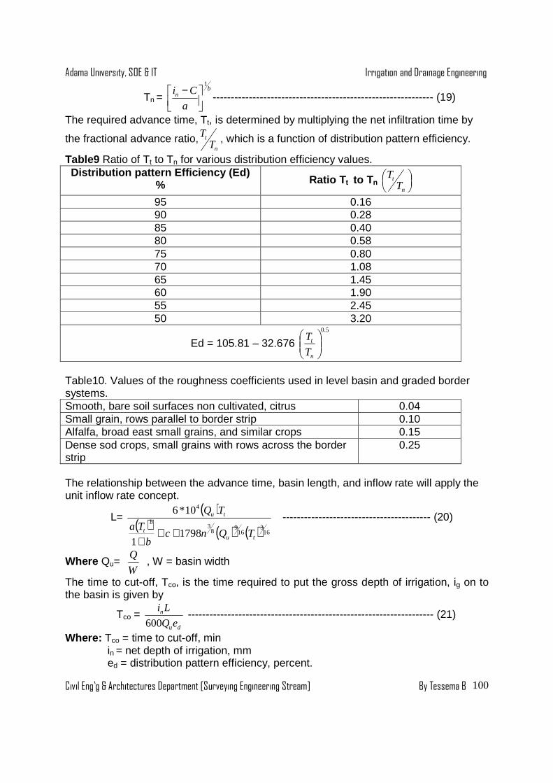
Adama University, SOE & IT Irrigation and Drainage Engineering
Civil Eng’g & Architectures Department [Surveying Engineering Stream] By Tessema B
100
Tn = b
n
a
Ci1
−------------------------------------------------------------- (19)
The required advance time, Tt, is determined by multiplying the net infiltration time by
the fractional advance ratio,n
tT
T , which is a function of distribution pattern efficiency.
Table9 Ratio of Tt to Tn for various distribution efficiency values. Distribution pattern Efficiency (Ed)
% Ratio T t to Tn
n
tT
T
95 0.16 90 0.28 85 0.40 80 0.58 75 0.80 70 1.08 65 1.45 60 1.90 55 2.45 50 3.20
Ed = 105.81 – 32.676 5.0
n
t
T
T
Table10. Values of the roughness coefficients used in level basin and graded border systems. Smooth, bare soil surfaces non cultivated, citrus 0.04 Small grain, rows parallel to border strip 0.10 Alfalfa, broad east small grains, and similar crops 0.15 Dense sod crops, small grains with rows across the border strip
0.25
The relationship between the advance time, basin length, and inflow rate will apply the unit inflow rate concept.
L= ( )
( ) ( ) ( ) 163
169
83
4
17981
10*6
tu
bt
tu
TQncb
Ta
TQ
+++
----------------------------------------- (20)
Where Qu= W
Q , W = basin width
The time to cut-off, Tco, is the time required to put the gross depth of irrigation, ig on to the basin is given by
Tco = du
n
eQ
Li
600 -------------------------------------------------------------------- (21)
Where: Tco = time to cut-off, min in = net depth of irrigation, mm ed = distribution pattern efficiency, percent.

Adama University, SOE & IT Irrigation and Drainage Engineering
Civil Eng’g & Architectures Department [Surveying Engineering Stream] By Tessema B
101
The maximum depth of flow in the basin, dmax, is an important parameter in basin design in that it governs the minimum ridge height. The ridge height should be equal to 1.25 times the maximum depth of flow and the ridge should have a maximum side slope ratio of 2.5:1 dmax = 2250 n3/8 Qu 9
/16 Tco 3/16 -------------------------------------------------------- (22)
Where dmax = maximum flow depth, mm Example Given the following information Intake family If = 0.5 Targeted distribution pattern efficiency ed = 80% Unit flow rate Qu = 0.005 m2/s Net irrigation depth in = 100mm Roughness coefficient n = 0.15 Assuming, 100 percent application efficiency, compute the net infiltration time, basin length, time – to – cut off, and maximum depth of flow. Solution 6.1.5.2. Graded Border System Design Graded border systems are similar in concept to level basin systems except that there is a slope down the border and there may be limited cross slope. Graded border systems may be more conveniently applied to soils of limited depth than level basin systems because of reduced leveling requirements. Graded border systems are most applicable to soils with moderately low to moderately high in take rates. This method is best suited to lands with slopes less than 0.5%. It can be used on lands of slopes up to 2% for non-grassy crops and up to approximately 4%for sod crops. Hydraulic Relationships The hydraulic relationships applied are complicated Relative to level basins in that the water applied is continuously moving down slope. The hydraulic relationships are derived by consideration of the continuity relationship, Manning's equation and the volume of a section with a triangular cross-sectional shape may approximate the assumption that the amount of water infiltrated in to the soil as the recession curve moves down the field.
Graded border systems are designed on the principle that any point in the field should have water applied to it for a time equal to that required to infiltrate the net depth of irrigation. Recession lag time: - The time interval between cut-off water at the head of the filed and the disappearance of water at the head of the field.

Adama University, SOE & IT Irrigation and Drainage Engineering
Civil Eng’g & Architectures Department [Surveying Engineering Stream] By Tessema B
102
Time to cut-off, Tco = Tn - Trl
The term high gradient borders is used to denote borders with a surface slope greater then
approximately 0.004m/m.In such borders, the water surface slope is assumed equal to the
field slope and the normal flow depth, that is, the depth of flow under conditions of uniform
flow is assumed equal to the depth of flow at the head of the border. Under such conditions,
the recession lag time is given by:
6.1
2.12.0
120S
nQT u
rc ---------------------------------------------------------------------- (23)
Where, Trl = recession lag time, min Qu = unit flow rate, m2/s N= Manning’s roughness coefficient S = surface slope, m/m
For low gradient borders with surface slopes less than 0.004m/m
Tre = 6.1
5.088.0
175.0
2.12.0
0094.0120
+
ST
nQS
nQ
n
u
u ----------------------------------------------------------- (24) Tn =
net infiltration time, min The inflow rate per unit width of border strip is given by-
Qu= ( )edTT
Li
rln
n
−00167.0
----------------------------------------------------------------------- (25)
Where: In = net depth of irrigation
L = border length, m ed= distribution efficiency, %
The maximum depth of flow in the in the border strip is determined by the border ridge height. The border ridge height is normally established at 1.25 times the maximum flow depth. Maximum flow depths of less than 150 mm are generally acceptable. In erosion resistant soil, flow depths in the range of 200mm may be acceptable.
Normal depth for uniform flow, (mm)
3.0
6.06.0100
S
nQd u
h = --------------------------------------------------------------------- (26)
For high gradient border dn= 2454 (Trl)
0.1875 Qu 0.5625 n 0.1875 --------------------------------------------- (27) For low gradient border
The maximum flow rate criterion has been established to have a non – erosive stream size.

Adama University, SOE & IT Irrigation and Drainage Engineering
Civil Eng’g & Architectures Department [Surveying Engineering Stream] By Tessema B
103
Qumax =
75.0
410*765.1
S
−
----------------------------------------------------------------- (29) for
alfalfa and small grains
Qumax = 75.0
410*53.3
S
−
------------------------------------------------------------------- (30)
For dense crops, posture A minimum depth of flow criterion is required to ensure that the water stream is large enough to spread over the entire border.
Qumin =n
LS 5.0610*95.5 −
--------------------------------------------------------------- (31)
The theoretical relationship for maximum slope is given by
Smax = ( )
n
renunax
i
TTedQ
00167.0
− ------------------------------------------------------ (32) Ed in %
6.2 Pressurized Irrigation
6.2.1 Introduction Application of water to the cropped land can be done in different forms in addition to the natural rainfall. It can be applied through surface irrigation methods that deliver water through channels with aid of gravity action. The other application pattern may be through pressurized irrigation, which delivers water under high pressure to the point of interest. With this respect, either a power supply system or an optimum elevation difference between the critical points to create suitable head for the water to flow is required. Water sources, Energy sources (Gravity, Mechanical, Internal combustion) and distribution network (pipe or canal) are basic irrigation components. 6.2.2. Sprinkler Irrigation 6.2.2.1 General
Sprinkler irrigation is a method of applying water to the surface of the soil in the form of a spray, which is similar to natural rainfall. This method of irrigation was started at about 1900. The first agricultural sprinkler systems were an outgrowth of city lawn sprinkling. Before 1920 sprinkling was limited to tree crops, nurseries and orchards. Most of these systems were stationary overhead-perforated pipe installations or stationary over tree systems with rotating sprinklers. These systems were expensive to install but often fairly inexpensive to operate. Portable sprinkler systems developed with the introduction of light weight steel pipe and quick couplers in the early 1930`s, resulted in reduction of equipment cost and increased number of sprinkler installation. The number of sprinkler installations has increased rapidly since 1950 owing to the development of more efficient sprinklers, lightweight aluminum pipe, more efficient pumps, and to the wide spread distribution of low cost electrical power and fuels for internal combustion engines. Sprinklers have been used on all soil types and on lands of widely different topography and slopes and for many crops.

Adama University, SOE & IT Irrigation and Drainage Engineering
Civil Eng’g & Architectures Department [Surveying Engineering Stream] By Tessema B
104
Water is distributed through a system of pipes usually by pumping. It is then sprayed into the air through sprinklers so that it breaks up into small water drops, which fall to the ground. The pump supply system, sprinklers and operating conditions must be designed to enable a uniform application of water.
6.2.2.2 Adaptability of Sprinkler Irrigation
Some of the conditions, which favor sprinkler irrigation, are as follows. • Soils too porous for good distribution by surface methods • Shallow soils the topography of which prevents proper leveling for surface
irrigation methods • Land having steep slopes and easily erodable soils • Irrigation stream too small to distribute water efficiently by surface irrigation • Undulating land too costly too level sufficiently for good surface irrigation • Land needs to be brought in to top production quality. Sprinkler systems can be
designed and installed quickly • Soils with low water holding capacities and shallow rooted crops, which require
frequent irrigation • Automation and mechanization are practical. • Labor available for irrigation is either not experienced in surface methods of
irrigation or is unreliable, good surface irrigation requires trained reliable labor • Higher application efficiency can be achieved by properly designed and
operated systems.
6.2.2.3 Other uses of Sprinkler irrigation
Sprinkler systems have several secondary agricultural uses, which are important in addition to the primary use for distributing irrigation water to be stored in the soil. Light frequent irrigations so easily managed by using sprinklers, are helpful in many situations, such as, shallow rooted crops, germination of new plants, control of soil temperature and humidity.
The other uses of sprinkler irrigation are:
• Frost protection • Application of fertilizers , pesticides and soil amendments • Crop cooling
6.2.2.4 Sprinkler Irrigation versus Surface irrigat ion When comparing sprinkler and surface methods of irrigation, the following points should be considered:
Sprinkler systems can be designed so that less interference with cultivation and other farming operations occurs and less land is taken out of production than with surface methods.
Frequent and small depth of water can readily be applied by sprinkler systems.
Adama University, SOE & IT Irrigation and Drainage Engineering
Civil Eng’g & Architectures Department [Surveying Engineering Stream] By Tessema B
105
Higher water application efficiency can normally be obtained by sprinkler irrigation.
For areas requiring in frequent irrigation, sprinkler irrigation can be provided at a lower capital investment per acre of land irrigated than can surface irrigation.
Water measurement is easier with sprinkler than with surface methods. Whenever water can be delivered to the field under gravity irrigation,
sprinkler irrigation is particularly attractive. When domestic and Irrigation water come from the same source, a common
distribution line can be frequently used.
6.2.2.5 Limitations of sprinkler Irrigation:
• Wind distorts sprinkler pattern and causes uneven distribution of water • Ripened soft fruits may be affected by spraying water • Water must be clean and free of sand, debris and large amount of dissolved
salts • High initial investment as compared to surface irrigation • High power requirements • Fine textured soils with slow infiltration rate can not be irrigated efficiently in hot
windy areas • In areas of high temperature and high wind velocity, considerable evaporation
losses of water may take place
6.2.2.6 Types of sprinklers and Sprinkler systems Various types of sprinkler systems have been developed in response to economic and labor conditions, topographic conditions, special water application needs and the availability of water and land resources. Sustained development of sprinkler system began in the Pacific Northwest of the United States where land and water resources were available for irrigation along with low cost hydroelectric power. Several types of sprinkler irrigation systems will be introduced here. 1. Based on the arrangement for spraying irrigation water sprinklers may be classified as fixed nozzles attached to the pipe, perforated pipe, and rotating sprinklers. 1. Fixed Nozzle: Parallel pipes are installed at about 15 meters apart and supported on rows of posts. Water is discharged at right angles perpendicularly from the pipeline. The entire 15 m width between pipelines may be irrigated by turning the pipes through about 135°. 2. Perforated sprinkler: Generally, application rates exceeding 20 mm/hr for this system and pressure heads less than 25m, often as low as 7m. They do not cover a very wide strip. 3. Rotating sprinklers: Extensively used due to its ability to apply water at a slower rate. It uses relatively large nozzle openings, which are favorable in water containing silt, and debris since less stoppage of sprinklers is experienced. Application rates less
Adama University, SOE & IT Irrigation and Drainage Engineering
Civil Eng’g & Architectures Department [Surveying Engineering Stream] By Tessema B
106
than 2 mm/hr are possible with sprinklers (advantageous for soils with low infiltration rates). Pressure heads vary from 20m to 70m for large units. 2. Classification based on the method of developing pressure:
• Pump powered system • Gravity sprinkler system • Hybrid systems (Pumps + Gravity)
3. Classification based on portability and make-up of units: Sprinkler system may be classified broadly as conventional systems (Periodic move and fixed systems) and mobile sprinkler machines (periodic move and continuous move system. 1. Conventional system ( Periodic move and fixed sy stems) Different types under this group based on portability and mobility of the different components are indicated.
• Permanent system • Solid set system • Portable system • Hand move (semi portable system)
6.2.2.7 Sprinkler System Components
A typical sprinkler irrigation system consists of the following components:
• Pressure generating units(Pump unit) • Water carrier units (Mainlines , sub mainlines, Laterals) • water delivery units (riser pipes and Sprinklers) • Quality improvement sub units ( Screens , Desilting-basins) • Ancillary units ( Fertilizer and other chemical applicator)
The pump unit is usually a centrifugal pump, which takes water from the source and provides adequate pressure for delivery into the pipe system.
1. Mainline : a line between the source of pressurized water and the point at which water is delivered to the field is the next component. Generally, the mainline is buried or aboveground pipeline. In the linear move system, the mainline can be an open channel and requires a pressurizing device, pump. 2. Lateral line : This comes out of the mainline to deliver water to the sprinkler nozzles. The position of the lateral may be permanent, as in a solid set, or moveable as in the hand move and side- roll systems. The spacing between the successive positions of the lateral along the mainline spacing and is designated as Sm. The distance between sprinkler nozzles along a lateral is termed as the lateral spacing and designated as Sl.

Adama University, SOE & IT Irrigation and Drainage Engineering
Civil Eng’g & Architectures Department [Surveying Engineering Stream] By Tessema B
107
To get a uniform rate of water application, the nozzle size, nozzle spacing or both are varied along the length of the pivot arm. The spray area, which is wet by each sprinkler nozzle at a particular operating pressure, is designated as the wetted diameter, DW. The wetted diameters are overlapped along the lateral to promote a uniform distribution of water application.
A common problem with sprinkler irrigation is the large labor force needed to move the pipes and sprinklers around the field. In some places, such labors may not be available and may be costly. To overcome this problem many mobile systems have been developed such as the hose reel rain gun and the center pivot.
6.2.2.8 Fertilizer applicator:
Soluble chemical fertilizers can be injected in to the sprinkler system; the fertilizer is easily placed at the desired depth in a soluble and readily available form to plants, with out any danger of being leached away. The two operations, irrigation and fertilizer application, are done simultaneously thus saving the labor required for fertilizer application.
Fertilizer can be introduced in to the system either through the suction side of the pump via a pipe and regulated by a valve, another pipe is connected from the discharge side of the pump to the fertilizer container for the required water supply in the tank or a venture fixed in the mainline creates a differential pressure and allows the fertilizer solution to flow in the main water line. In some designs, the applicator could have separate injection pump.
Introducing fertilizers through the suction side of the pump via the pipe is simpler but pump impellers are likely to be corroded due to the fertilizer solution, unless the impellers are made of corrosion resistant materials. When applying the fertilizer through the sprinkler system, it is desirable to operate the system long enough with out turning on fertilizer injector valve, to wet the soil and the plant foliage. The ratio of water to fertilizer by weight is about 30:1 and timed to be injected with in half an hour. After injection, the system has to operate for about 20- 30 minutes to flush it out from toxic effects of the fertilizer solution.
6.2.2.9 Desilting basin (Settlement reaches):
Desilting basins may be required to trap and or suspended silts when the water comes from streams, open ditches or well water having silt. Some times desilting basins and debris screen are built as a combination structure. Desilting basin should be large enough to provide protection for at least one full day.
1. Debris screen:
Debris screen are usually needed when surface water is used as the source of irrigation. The function of screens is to keep the system free of trash that might plug the sprinkles nozzles. Screens should be fine enough to catch weed seeds and other small
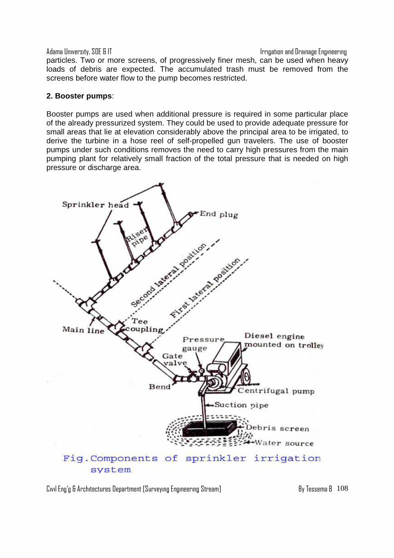
Adama University, SOE & IT Irrigation and Drainage Engineering
Civil Eng’g & Architectures Department [Surveying Engineering Stream] By Tessema B
108
particles. Two or more screens, of progressively finer mesh, can be used when heavy loads of debris are expected. The accumulated trash must be removed from the screens before water flow to the pump becomes restricted.
2. Booster pumps :
Booster pumps are used when additional pressure is required in some particular place of the already pressurized system. They could be used to provide adequate pressure for small areas that lie at elevation considerably above the principal area to be irrigated, to derive the turbine in a hose reel of self-propelled gun travelers. The use of booster pumps under such conditions removes the need to carry high pressures from the main pumping plant for relatively small fraction of the total pressure that is needed on high pressure or discharge area.
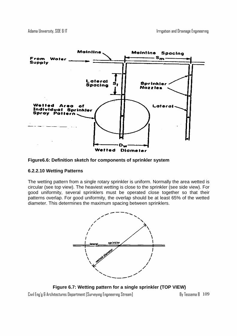
Adama University, SOE & IT Irrigation and Drainage Engineering
Civil Eng’g & Architectures Department [Surveying Engineering Stream] By Tessema B
109
Figure6.6: Definition sketch for components of spri nkler system
6.2.2.10 Wetting Patterns
The wetting pattern from a single rotary sprinkler is uniform. Normally the area wetted is circular (see top view). The heaviest wetting is close to the sprinkler (see side view). For good uniformity, several sprinklers must be operated close together so that their patterns overlap. For good uniformity, the overlap should be at least 65% of the wetted diameter. This determines the maximum spacing between sprinklers.
Figure 6.7: Wetting pattern for a single sprinkler (TOP VIEW)

Adama University, SOE & IT Irrigation and Drainage Engineering
Civil Eng’g & Architectures Department [Surveying Engineering Stream] By Tessema B
110
Figure6.8: Wetting pattern for a single sprinkler ( SIDE VIEW)
The uniformity of sprinkler applications can be affected by wind and water pressure. Spray from sprinklers is easily blown about by even a gentle breeze and this can seriously reduce uniformity. To reduce the effects of wind the sprinklers can be positioned more closely together.
Figure6.9: Overlapping-wetting pattern.
6.2.2.11 Application Rates The application rate to the soil surface must therefore be less than the intake rate of the soil. The lower limit of the application rate must take in to account that there will be safe evaporation and wind drift of water from the nozzle. Thus, the discharge rate of the nozzle should be high enough that adequate water remains after evaporation and wind drift to enable a reasonable amount of water to be infiltrated in to the root zone.
The gross application rate,
dg=ml SS
q
.
*360------------------------------------------------------------------------- (32)
Where, dg = gross application rate, cm/h
Wetted Depth
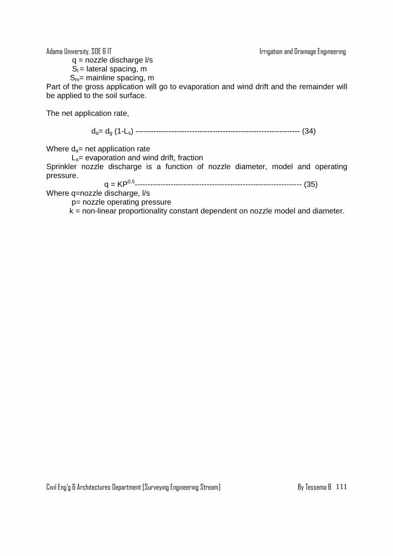
Adama University, SOE & IT Irrigation and Drainage Engineering
Civil Eng’g & Architectures Department [Surveying Engineering Stream] By Tessema B
111
q = nozzle discharge l/s Sl = lateral spacing, m Sm= mainline spacing, m Part of the gross application will go to evaporation and wind drift and the remainder will be applied to the soil surface. The net application rate, da= dg (1-Ls) ---------------------------------------------------------------- (34) Where da= net application rate Ls= evaporation and wind drift, fraction Sprinkler nozzle discharge is a function of nozzle diameter, model and operating pressure. q = KP0.5----------------------------------------------------------------- (35) Where q=nozzle discharge, l/s p= nozzle operating pressure k = non-linear proportionality constant dependent on nozzle model and diameter.

Adama University, SOE & IT Irrigation and Drainage Engineering
Civil Eng’g & Architectures Department [Surveying Engineering Stream] By Tessema B
112
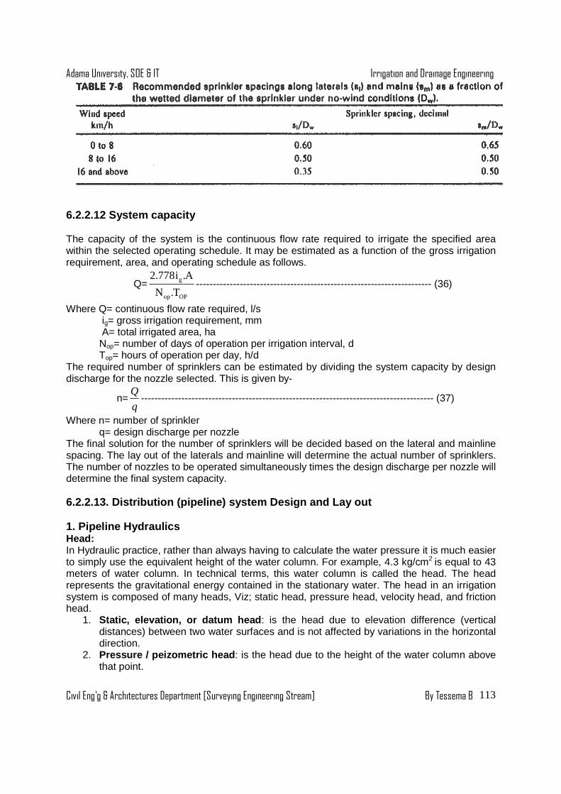
Adama University, SOE & IT Irrigation and Drainage Engineering
Civil Eng’g & Architectures Department [Surveying Engineering Stream] By Tessema B
113
6.2.2.12 System capacity The capacity of the system is the continuous flow rate required to irrigate the specified area within the selected operating schedule. It may be estimated as a function of the gross irrigation requirement, area, and operating schedule as follows.
Q=OPop
g
T.N
A.i778.2---------------------------------------------------------------------- (36)
Where Q= continuous flow rate required, l/s ig= gross irrigation requirement, mm A= total irrigated area, ha Nop= number of days of operation per irrigation interval, d Top= hours of operation per day, h/d The required number of sprinklers can be estimated by dividing the system capacity by design discharge for the nozzle selected. This is given by-
n=q
Q--------------------------------------------------------------------------------------- (37)
Where n= number of sprinkler q= design discharge per nozzle The final solution for the number of sprinklers will be decided based on the lateral and mainline spacing. The lay out of the laterals and mainline will determine the actual number of sprinklers. The number of nozzles to be operated simultaneously times the design discharge per nozzle will determine the final system capacity. 6.2.2.13. Distribution (pipeline) system Design and Lay out 1. Pipeline Hydraulics Head: In Hydraulic practice, rather than always having to calculate the water pressure it is much easier to simply use the equivalent height of the water column. For example, 4.3 kg/cm2 is equal to 43 meters of water column. In technical terms, this water column is called the head. The head represents the gravitational energy contained in the stationary water. The head in an irrigation system is composed of many heads, Viz; static head, pressure head, velocity head, and friction head.
1. Static, elevation, or datum head : is the head due to elevation difference (vertical distances) between two water surfaces and is not affected by variations in the horizontal direction.
2. Pressure / peizometric head : is the head due to the height of the water column above that point.

Adama University, SOE & IT Irrigation and Drainage Engineering
Civil Eng’g & Architectures Department [Surveying Engineering Stream] By Tessema B
114
3. Velocity head : is the energy required to accelerate water at a point from rest. The velocity head in an irrigation system is very small because velocity seldom greater than 2.5m/s.
4. Friction head : is the energy required for the water to flow between two points overcoming friction .For a given sprinkler the operating pressure requirement is fixed. The static head, which is a function of the topography, is also fixed. What we need is the friction loss.
Hydraulic Grade line: The Hydraulic grade line (HGL) represents the energy level because of friction losses in the pipeline. For any constant flow through a pipe, there is a specific and constant HGL. The vertical distance from the pipeline to the HGL is a measure of pressure head (i.e. energy) and the difference between the HGL and SWL represents the head lost due to friction, hf. The HGL any pipeline’s outlet is called the residual head and represents the excess water pressure over the atmospheric pressure. The residual pressure at the nozzle outlet in sprinkler system is called the operating pressure. Lateral System Design The equation q = kp0.5 indicates that nozzle discharge is a function of the square root of the nozzle operating pressure. Previous relationships for uniformity, gross application rate, and net application rate all assumed that each nozzle was discharging at same flow rate. In all but the rarest conditions, it is not possible to have the same operating pressure available for every nozzle on a lateral. The concept of lateral design is therefore based on limiting pressure differences along a lateral so the variation of nozzle discharge is with in acceptable range. The usual criterion applied for the design of laterals is that the difference in nozzle discharge along a single lateral is less than ±10percent. To accomplish this goal, the difference in nozzle operating pressure is typically constrained to a variation of less than ± 20% along the lateral. The procedure for lateral design requires that a balance be developed between the length of the lateral, the head loss due to friction in the lateral, and the change in elevation head due to topographic effects. These factors are kept in balance so the pressure variation between the two critical sprinklers on a lateral is limited to ±20 % The governing equation for the maximum allowable head loss due to friction between the two
critical sprinklers is given by ( )
l
eaL
HHH
−=
θ ---------------------------------------- (38)
Where HL = maximum allowable head loss due to friction, m/m θ = maximum allowable pressure difference, fraction Ha = nozzle design pressure expressed as head, m He = increase in elevation in direction of water flow between the two critical Sprinklers, m l = distance between the two critical sprinkler, m Note: He is negative for downhill sloping laterals.
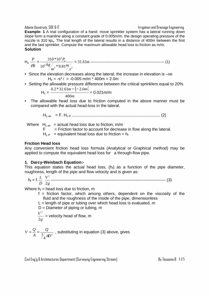
Adama University, SOE & IT Irrigation and Drainage Engineering
Civil Eng’g & Architectures Department [Surveying Engineering Stream] By Tessema B
115
Example- 1 A trial configuration of a hand- move sprinkler system has a lateral running down slope form a mainline along a constant grade of 0.005m/m. the design operating pressure of the nozzle is 310 kpa. The trial length of the lateral results in a distance of 400m between the first and the last sprinkler. Compute the maximum allowable head loss to friction as m/m. Solution
Ha m
sm
mkg
P
g
P a 61.3181.9*10
10*310
233
3
==ρ
----------------------------------------------------------- (1)
• Since the elevation decreases along the lateral, the increase in elevation is –ve He = -s*l = -0.005 m/m * 400m = 2.0m
• Setting the allowable pressure difference between the critical sprinklers equal to 20%.
Hc = ( )
m
mm
400
0.261.31*2.0 −−= 0.021m/m
• The allowable head loss due to friction computed in the above manner must be compared with the actual head-loss in the lateral.
HL-ac = F. HL-P ------------------------------------------------------------------------------------------------- (2)
Where HL-ac = actual head loss due to friction, m/m F = Friction factor to account for decrease in flow along the lateral. HL-P = equivalent head loss due to friction = hf
Friction Head loss Any convenient friction head loss formula (Analytical or Graphical method) may be applied to compute the equivalent head loss for a through-flow pipe. 1. Darcy-Weisbach Equation:- This equation states the actual head loss, (hf) as a function of the pipe diameter, roughness, length of the pipe and flow velocity and is given as:
hf = f.D
L
g
V
2
2
------------------------------------------------------------------------------------ (3)
Where hf = head loss due to friction, m f = friction factor, which among others, dependent on the viscosity of the
fluid and the roughness of the inside of the pipe, dimensionless L = length of pipe or tubing over which head loss is evaluated, m D = Diameter of piping or tubing, m
g
V
2
2
= velocity head of flow, m
2
41 D
Q
A
QV
π== , substituting in equation (3) above, gives

Adama University, SOE & IT Irrigation and Drainage Engineering
Civil Eng’g & Architectures Department [Surveying Engineering Stream] By Tessema B
116
5
2
2
8
D
LQ
g
fh f π
= , therefore, hf LD
Q ≈≈≈5
2 1 , doubling the diameter of the pipe reduce
hf by 32.
The dimensionless friction factor, f that is given by the equation =f
g
V
D
L
h f
2
2 is
estimated using equations or Moody Diagram. From the Moody diagram, it is evident that the friction factor is a linear function of Reynolds number and in laminar flow and a nonlinear function of the Reynolds number in partially turbulent flow or transition zone. In fully turbulent flow, the friction factor is constant regardless of the value of the Reynolds number. A flow regime cannot be maintained in the unstable or critical zone in a field installation. This zone of flow regime is not important in design situations other than the fact that it is to be avoided because the flow is unstable.
f = Re
64 , for laminar flow
The friction factor, f for turbulent flow can be estimated using the Colebrook‘s equation.
+
∈
−=f
Df Re
51.2
7.3log2
1--------------------------------------------------------------- (4)
Where Re =ν
VD , Reynolds Number, dimensionless
∈ = wall roughness of the pipe ν =Kinematic Viscosity of the fluid, m2/s 2. Hazen – William’s equation Many empirical formulas are used for pipe flow analysis in engineering practice. These formulas have been obtained from experiments on flow of water under turbulent conditions. Use of such formulas for flow of other liquids is therefore not likely to give reliable results. The Hazen- Williams formula is typical of such formula and is probably the most widely used. The formula is written as:
hf = 87.4
852.1
DC
QKL
------------------------------------------------------------------------------(5)
Where: hf =friction loss expressed as head, m K = conversion constant = 1.22*1010
L = length f pipe, m Q = Volumetric flow rate, l/s C = Hazen – William friction coefficient (C= 135 for aluminum pipes) D = Pipe diameter, mm
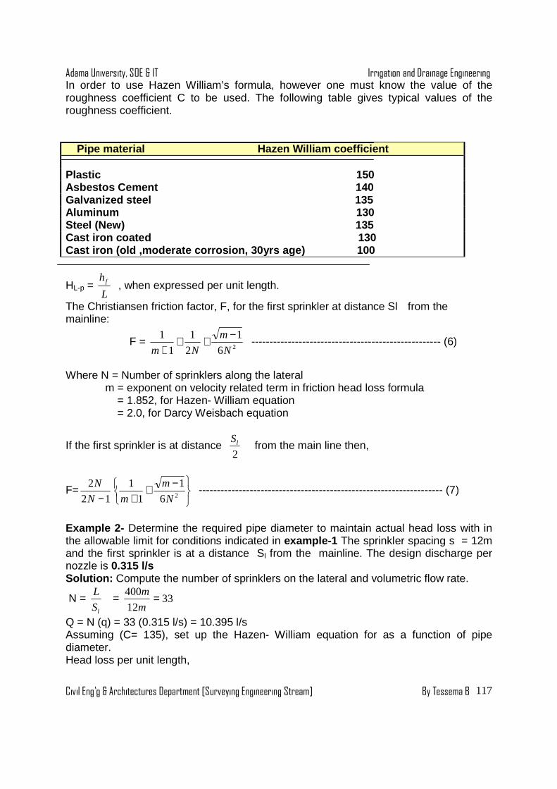
Adama University, SOE & IT Irrigation and Drainage Engineering
Civil Eng’g & Architectures Department [Surveying Engineering Stream] By Tessema B
117
In order to use Hazen William’s formula, however one must know the value of the roughness coefficient C to be used. The following table gives typical values of the roughness coefficient.
Pipe material H azen William coefficient
Plastic 150 Asbestos Ceme nt 140 Galvanized steel 135 Aluminum 130 Steel (New) 135 Cast iron coated 130 Cast iron (old ,moderate corrosion, 30yrs age) 100
HL-p = L
h f , when expressed per unit length.
The Christiansen friction factor, F, for the first sprinkler at distance Sl from the mainline:
F = 26
1
2
1
1
1
N
m
Nm
−+++
---------------------------------------------------- (6)
Where N = Number of sprinklers along the lateral m = exponent on velocity related term in friction head loss formula = 1.852, for Hazen- William equation = 2.0, for Darcy Weisbach equation
If the first sprinkler is at distance 2
lS from the main line then,
F=12
2
−N
N
−+
+ 26
1
1
1
N
m
m ------------------------------------------------------------------- (7)
Example 2- Determine the required pipe diameter to maintain actual head loss with in the allowable limit for conditions indicated in example-1 The sprinkler spacing s = 12m and the first sprinkler is at a distance Sl from the mainline. The design discharge per nozzle is 0.315 l/s Solution: Compute the number of sprinklers on the lateral and volumetric flow rate.
N = lS
L = 33
12
400 =m
m
Q = N (q) = 33 (0.315 l/s) = 10.395 l/s Assuming (C= 135), set up the Hazen- William equation for as a function of pipe diameter. Head loss per unit length,
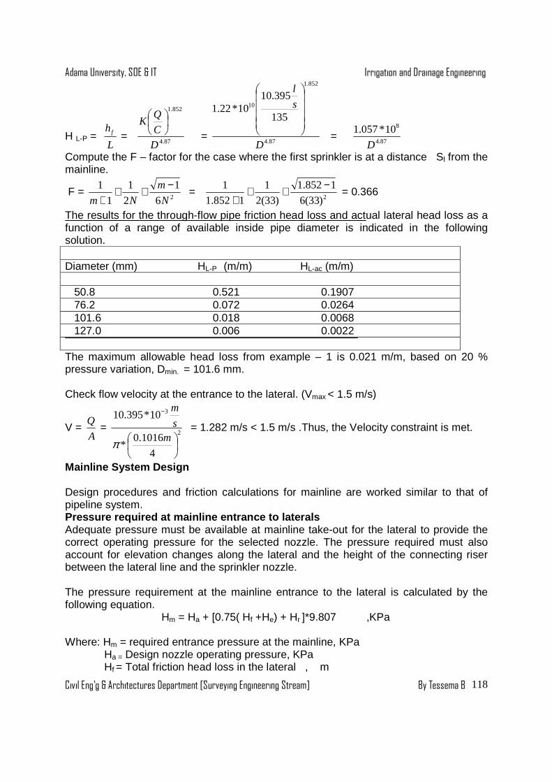
Adama University, SOE & IT Irrigation and Drainage Engineering
Civil Eng’g & Architectures Department [Surveying Engineering Stream] By Tessema B
118
H L-P = L
h f = 87.4
852.1
D
C
QK
= 87.4
852.1
10
135
395.1010*22.1
D
s
l
= 87.4
810*057.1
D
Compute the F – factor for the case where the first sprinkler is at a distance Sl from the mainline.
F = 26
1
2
1
1
1
N
m
Nm
−+++
= 2)33(6
1852.1
)33(2
1
1852.1
1 −+++
= 0.366
The results for the through-flow pipe friction head loss and actual lateral head loss as a function of a range of available inside pipe diameter is indicated in the following solution. Diameter (mm) HL-P (m/m) HL-ac (m/m) 50.8 0.521 0.1907 76.2 0.072 0.0264 101.6 0.018 0.0068 127.0 0.006 0.0022 The maximum allowable head loss from example – 1 is 0.021 m/m, based on 20 % pressure variation, Dmin. = 101.6 mm. Check flow velocity at the entrance to the lateral. (Vmax < 1.5 m/s)
V = A
Q =
2
3
4
1016.0*
10*395.10
−
ms
m
π = 1.282 m/s < 1.5 m/s .Thus, the Velocity constraint is met.
Mainline System Design
Design procedures and friction calculations for mainline are worked similar to that of pipeline system. Pressure required at mainline entrance to laterals Adequate pressure must be available at mainline take-out for the lateral to provide the correct operating pressure for the selected nozzle. The pressure required must also account for elevation changes along the lateral and the height of the connecting riser between the lateral line and the sprinkler nozzle. The pressure requirement at the mainline entrance to the lateral is calculated by the following equation. Hm = Ha + [0.75( Hf +He) + Hr ]*9.807 ,KPa Where: Hm = required entrance pressure at the mainline, KPa Ha = Design nozzle operating pressure, KPa Hf = Total friction head loss in the lateral , m
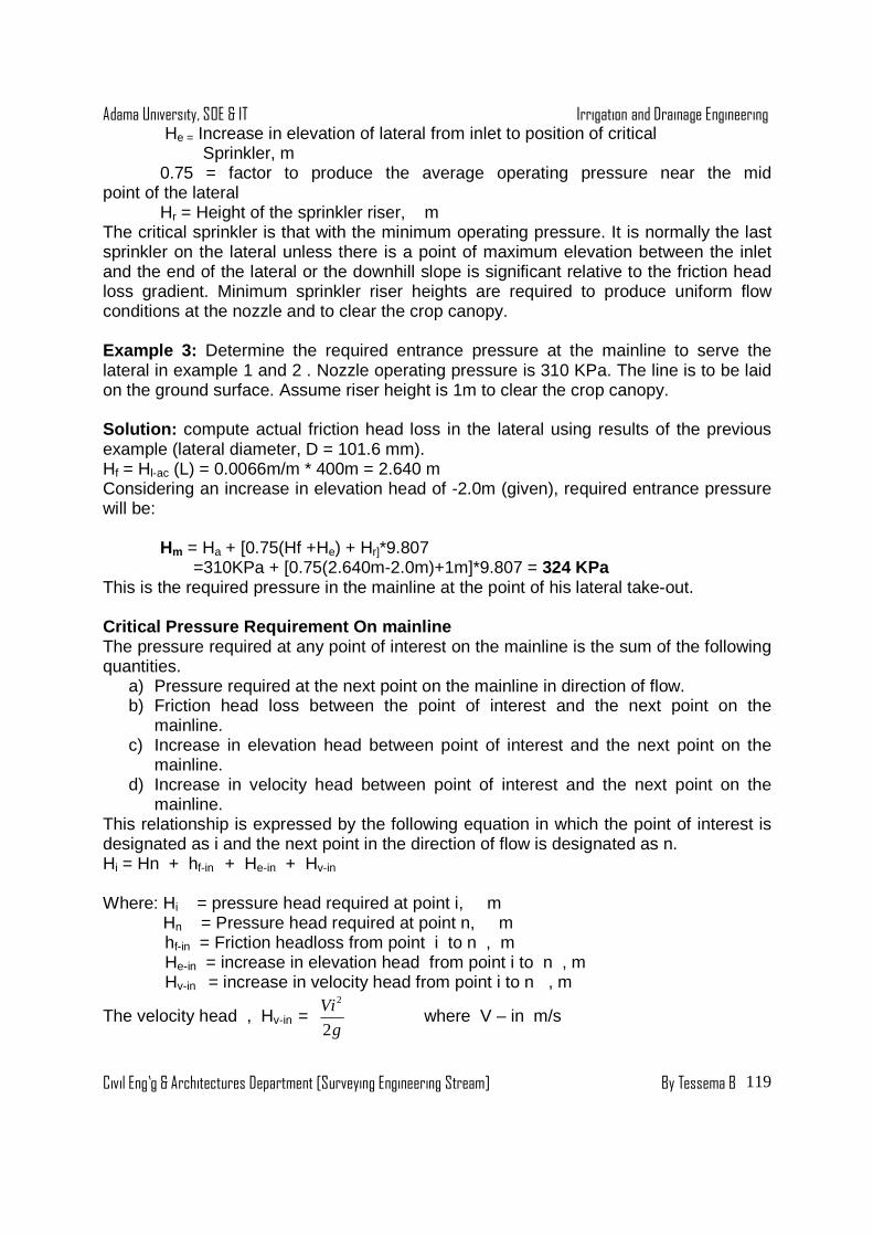
Adama University, SOE & IT Irrigation and Drainage Engineering
Civil Eng’g & Architectures Department [Surveying Engineering Stream] By Tessema B
119
He = Increase in elevation of lateral from inlet to position of critical Sprinkler, m 0.75 = factor to produce the average operating pressure near the mid point of the lateral Hr = Height of the sprinkler riser, m The critical sprinkler is that with the minimum operating pressure. It is normally the last sprinkler on the lateral unless there is a point of maximum elevation between the inlet and the end of the lateral or the downhill slope is significant relative to the friction head loss gradient. Minimum sprinkler riser heights are required to produce uniform flow conditions at the nozzle and to clear the crop canopy. Example 3: Determine the required entrance pressure at the mainline to serve the lateral in example 1 and 2 . Nozzle operating pressure is 310 KPa. The line is to be laid on the ground surface. Assume riser height is 1m to clear the crop canopy. Solution: compute actual friction head loss in the lateral using results of the previous example (lateral diameter, D = 101.6 mm). Hf = Hl-ac (L) = 0.0066m/m * 400m = 2.640 m Considering an increase in elevation head of -2.0m (given), required entrance pressure will be: Hm = Ha + [0.75(Hf +He) + Hr]*9.807 =310KPa + [0.75(2.640m-2.0m)+1m]*9.807 = 324 KPa This is the required pressure in the mainline at the point of his lateral take-out. Critical Pressure Requirement On mainline The pressure required at any point of interest on the mainline is the sum of the following quantities.
a) Pressure required at the next point on the mainline in direction of flow. b) Friction head loss between the point of interest and the next point on the
mainline. c) Increase in elevation head between point of interest and the next point on the
mainline. d) Increase in velocity head between point of interest and the next point on the
mainline. This relationship is expressed by the following equation in which the point of interest is designated as i and the next point in the direction of flow is designated as n. Hi = Hn + hf-in + He-in + Hv-in
Where: Hi = pressure head required at point i, m Hn = Pressure head required at point n, m hf-in = Friction headloss from point i to n , m He-in = increase in elevation head from point i to n , m Hv-in = increase in velocity head from point i to n , m
The velocity head , Hv-in = g
Vi
2
2
where V – in m/s
Adama University, SOE & IT Irrigation and Drainage Engineering
Civil Eng’g & Architectures Department [Surveying Engineering Stream] By Tessema B
120
The velocity head are usually very small and can be neglected with out loss of accuracy. The calculation of the head required at any point i requires the calculation of the pressure required at the next point n. Therefore, pressure calculations are started at the end of the line and worked back towards the pump. The critical point on the mainline is the point with the highest-pressure requirement taking in to account all pressure losses starting from the pump. The pump must deliver adequate head at the critical point for the proper operation of the system. The pressure head required at the pump is equal to the sum of the following components.
a) Pressure head required at the critical point in the mainline. b) Total friction head loss from the pump to the critical point in the mainline. c) Elevation head from the water source to the critical point in the mainline. d) Friction head loss from the pumping water level to the centerline of the pump. e) Velocity head at the critical point in the mainline. The summation of these quantities equals the total dynamic head requirement of the pump. The total dynamic head required must theoretically be calculated for each point in the mainline, and the point with the highest requirement is the critical point.
In equation form the total dynamic head,
TDHi = Hi + hf-pi + He-si +Hf-s + g
Vi
2
2
Where: TDH = Total dynamic head required for point i, m hf-pi = Friction head loss from pump to point i , m He-si = increase in elevation from source to point i, m Hf –s = friction head loss on suction side of pump , m The pump must be able to produce the maximum calculated total dynamic head at the design flow rate to develop the required pressure distribution in the main line. If the pressure required at the critical point in the mainline is adequate all other points in the mainline with lower pressure requirements will have sufficient pressure. In some cases, development of adequate pressure at the critical point will produce exceedingly high pressure at other points in the distribution system. These high pressures could cause excessively high discharges in sprinkler laterals connected at these points. There are two correction procedures for this condition.
1. Installing pressure regulators at the lateral take-outs from the mainline 2. Adjusting the opening of the hydrant valve at the inlet to achieve the
same effect The regulators or valve adjustments maintain the pressure at the inlet to the lateral at the level computed above (pressure requirement at the entrance).This is the normal method of correction for high pressure in parts of the mainline on small or moderate size irrigation systems. In more extensive systems, it may be advisable to produce the advisable pressure at the critical points in stages. This is done by installing a booster pumps at intermediate locations in the mainline to produce the proper pressure head at the critical point. Use of booster pumps avoids the cost of producing high pressure in certain sections of the pipeline only to have it controlled by a pressure regulator.