irrigated areas discharge and sediment interaction case ...ijsrst.com/paper/942.pdf · sudan 2civil...

IJSRST16211 | 10 March 2017 | Accepted: 20 March 2017 | March-April-2017 [(2)3: 01-05 ]

© 2017 IJSRST | Volume 3 | Issue 3 | Print ISSN: 2395-6011 | Online ISSN: 2395-602X Themed Section: Science and Technology

1

Irrigated Areas Discharge and Sediment Interaction Case Study Roseires Dam

Nabela Hamed Elamein *1, Abbas Abd Alla1, Gassan Khalid2

*1Department of Water Resource Engineering, Sudan University of Science and Technology, Khartoum, Khartoum,

Sudan

*1Department of Water Resource Engineering, Sudan University of Science and Technology, Khartoum, Khartoum,

Sudan 2Civil Engineering, Yarmouk College, Khartoum, Khartoum, Sudan

ABSTRACT

Dams and reservoirs are constructed in rivers for multipurpose. Irrigation is always predominant. Irrigated

agriculture in Sudan produces about 50 % of the total crop production. There is always painstaking in removing

sediments from the irrigation network system. The objective of this study is to assess the relations among sediment

irrigated areas and discharge in Roseires Dam Reservoir. Dimensional analysis and SPSS models, in both simple

and multiple correlations were conducted. The simple correlation gave acceptable results with high correlation

coefficients. Complete set of dimensionless groups were obtained in the multiple regression correlation.

Examination of the results indicated good correlation with acceptable error.

Keywords : irrigation network, agricultural schemes, Buckingham pi theorem, SPSS

I. INTRODUCTION

Dams and reservoirs are constructed in rivers for flood

control, hydropower generation, irrigation, navigation,

water supply, fishing and recreation. Irrigation dams are

predominant. Sedimentation is one of the major

problems, which endangers the performance, and

sustainability of reservoirs.

Alarming rates of storage depletion have been reported

worldwide and especially in drought prone areas. Mean

yearly losses of 0.3% to 1.3% were reported in USA,

0.7 % to 1.5% in Turkey (Bechteler 1997), 1.67% in

Sudan and 1% worldwide (Mahmood 1987).

Agriculture is the most significant element in Sudanese

economy. Most of the important crops such as cotton,

wheat, sorghum, and groundnut are produced by

irrigation. Irrigated agriculture produces about 50 % of

the total crop production. In the year 1990, due to

siltation and reduced water availability, the Gezira

scheme (760 000 ha), was dropped to 57% as 326800 ha

were taken out of production (FAO report 1995a).

Depending on the annual sediment yield, quantities

ranging from 10 to 20 million m3 of sediment were

removed from the irrigation canals before the beginning

of the coming season (Adam, A.M. 1997). In brief, the

rate and magnitude of sedimentation in the new

reservoirs and its impact on surface water management

was received as a shock (Tan. Soon-Keat,

Guoliang2005). This impact has manifested in

progressive reduction in the irrigated areas of main crops

The prevailing problems affecting Roseires Dam are

several. They are mainly: Upstream downstream

sediment transportation, diminishing downstream

releases associated with decreasing and fluctuating

cultivated areas.

The main objective is to assess the impact of sediment

on irrigation water and optimization of use and

consumption of water for irrigation. Specific objectives:

Indication of interaction among discharge sediment and

cultivated areas. Suggest some recommendations to

measures that can be taken to reduce the amount of

deposited sediment.

International Journal of Scientific Research in Science and Technology (www.ijsrst.com)

113

II. METHODS AND MATERIAL

A. Area of Study

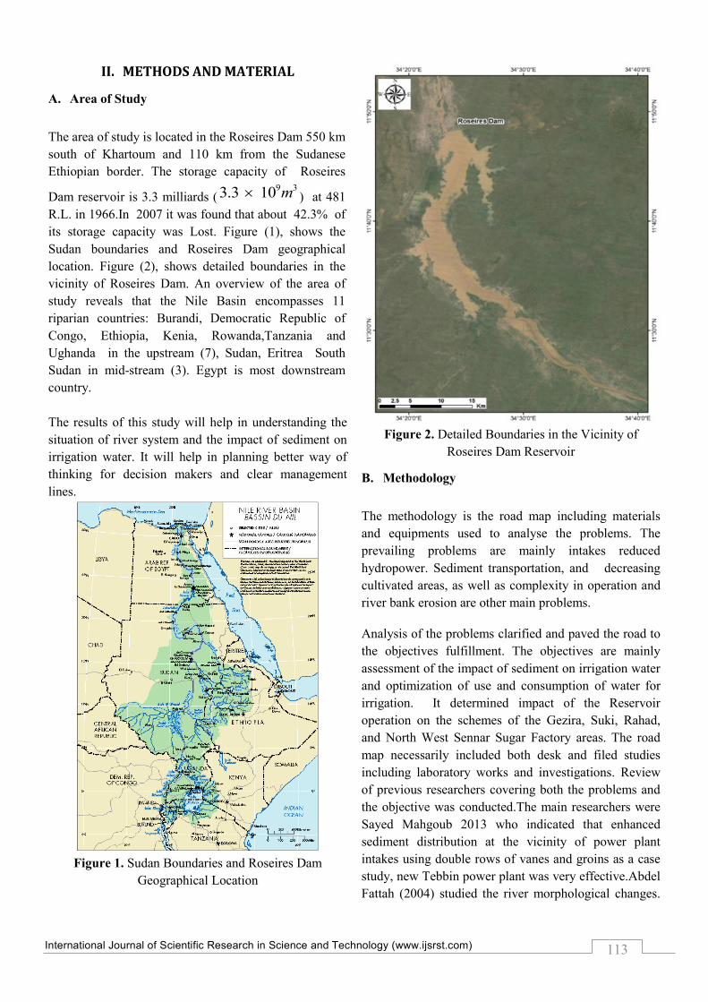
The area of study is located in the Roseires Dam 550 km

south of Khartoum and 110 km from the Sudanese

Ethiopian border. The storage capacity of Roseires

Dam reservoir is 3.3 milliards (9 33.3 10 m ) at 481

R.L. in 1966.In 2007 it was found that about 42.3% of

its storage capacity was Lost. Figure (1), shows the

Sudan boundaries and Roseires Dam geographical

location. Figure (2), shows detailed boundaries in the

vicinity of Roseires Dam. An overview of the area of

study reveals that the Nile Basin encompasses 11

riparian countries: Burandi, Democratic Republic of

Congo, Ethiopia, Kenia, Rowanda,Tanzania and

Ughanda in the upstream (7), Sudan, Eritrea South

Sudan in mid-stream (3). Egypt is most downstream

country.

The results of this study will help in understanding the

situation of river system and the impact of sediment on

irrigation water. It will help in planning better way of

thinking for decision makers and clear management

lines.

Figure 1. Sudan Boundaries and Roseires Dam

Geographical Location

Figure 2. Detailed Boundaries in the Vicinity of

Roseires Dam Reservoir

B. Methodology

The methodology is the road map including materials

and equipments used to analyse the problems. The

prevailing problems are mainly intakes reduced

hydropower. Sediment transportation, and decreasing

cultivated areas, as well as complexity in operation and

river bank erosion are other main problems.

Analysis of the problems clarified and paved the road to

the objectives fulfillment. The objectives are mainly

assessment of the impact of sediment on irrigation water

and optimization of use and consumption of water for

irrigation. It determined impact of the Reservoir

operation on the schemes of the Gezira, Suki, Rahad,

and North West Sennar Sugar Factory areas. The road

map necessarily included both desk and filed studies

including laboratory works and investigations. Review

of previous researchers covering both the problems and

the objective was conducted.The main researchers were

Sayed Mahgoub 2013 who indicated that enhanced

sediment distribution at the vicinity of power plant

intakes using double rows of vanes and groins as a case

study, new Tebbin power plant was very effective.Abdel

Fattah (2004) studied the river morphological changes.


114

He used two dimensional (2-D) numerical models and

investigated sediment distribution at El-Kurimat thermal

power plant intake. He revealed that using groins and

dredging upstream intake increased the flow ratio in

front of intake and diverts sediment away off it.Other

reviewers were AbdelHaleem (2008) Hassanpour and

Ayoubzadeh (2008), Yasir (2014) and (15) Ageel I.

Bushara. Aggradation degradation and scour:- was

reviewed by the researchers Black, Richard (2009-09-

21) ,and Hydraulic Engineering Circular No. 18 Manual

(HEC-18) was published by the Federal Highway

Administration (FHWA).The Assessment of Sediment

Impact and Optimized Consumption of Irrigation

Water : was reviewed by Islam Al Zayed1et.al and

Yasir(2013). Rouseires Dam Operation And

Maintenance Difficulties was reviewed by the consultant

Sir Alexander Gibb & Partners who proposed a manual

1973.Other reviewers are UNESCO Chair in Water

Resources, 2011). Dam Implementation Unit, 2012).The

main parameters reviewed were the river discharge and

the bathometric surveying.

C. Data Collection and Analysis

River engineering constructions are very expensive. At

the first stage of design, resort must be made to

theoretical approaches. If the whole design or part of it

can not be predicted by theory, it is accordingly

advisable to study the performance of the whole or part

of the prototype by means of a hydraulic model.

Generally, hydraulic models are of two types. Those

designed to solve a special hydraulic Those designed to

solve a special hydraulic problem as for example a

definite reach of a known river, and those designed for

research for establishing hydraulic laws applicable to

special problems within the field of river engineering.

The first type produces qualitative results only applicable

to known prototype river, while the second type produces

quantitative results applicable to any prototype involving

the same special problem with the same hydraulic laws.

Unfortunately, the former cannot be applied, because a

large hydraulic laboratory is needed which is not

available. Similarly, the latter cannot be applied because

of lack of sophisticated equipments usually needed in

such case. However simple conceptual mathematical

models using the standing computers strong SPSS

techniques can be applied.

In this study, using this technique the details of SPSS

Models facilities and analysis procedures are applied. A

complete set of data on hydrological and morphological

aspects events results are analysed and presented in the

form of graphs and tables. Simple correlation is

presented in table (1).

Table No.(1): Simple Correlation Among Power

Sediment and Water Requirements

Correlation High

Coefficient

Low

Coefficient

Discharge Power 0.9663, 0.0936

Discharge

Sediment

0.80016 0.695

Discharge water

Requirement

0.606 0.323

Using Dimensional Analysis, a property (A) , of any

phenomenon can be expressed in terms of all or some of

the (n), characteristic parameters of the phenomenon, in

a functional relation of the form:-

1 2 3 = , , ..... ------- 1 A nA x x x x

According to Backingham π theorem, the (n)

dimensional parameters will have a general equation

expressed as a function of (n-m) dimensionless π terms

parameter as given in the matrix form table (2).

Table No. (2): Matrix Form of Dimensional

Parameters

The above matrix is (3x15) matrix of rank(3).The

number of the dimensionless groups is the number of the

parameters(n), minus the rank of the matrix (r=3). The

number of the dimensionless π terms is

15 3 12

Choozing , , s sand W

as the selected determinant its

value is calculated as follows as given in table (3),of the

determinant taken from the matrix form of table (2).


115

Table No. (3): Determinant Taken From The Matrix

Table (2).

1 1 1 2 1 1 1 2 3

Again choosing , , s sand W

as the repeating variables,

and. solving for their coefficients 13 14 15, , k k and k in terms

of the other 1 12 kks k to

Gave the solution

13 1 2 4 5 6 8 9 10 11 122 2 2K K K K K K K K K K K

14 1 2 4 5 6 7 8 9 10 11 122 2 2 3 2k k k k k k k k k k k k

15 3 6 7 8 9 10 122 2k k k k k k k k

Substituting these values in the matrix give the solution

in table (4).

Hence as shown in table (4) ,the twelve (12),

dimensionless groups are calculated as given below

2

s1 2 3 42

s s

s

B A DV

W

2

s s5 6 7 8 s2 2

s s

d g W

W

s sW

2 2

s 50 s s9 10 11 122 3 2

s s

Q P

W W

s s

s

d Q

W

The total number of the the dimensionless groups will be

fourteen (14)

13 14 i

These equations can be put in the form

22 2 2

s s 500 2 2 2 2 3 2

, , , , , , , , , , , , , 2ss s s s s s s s s s

A

s s s s s s

QB A D d W W P d QV gi

W W W W W

The resulting equation is the equation developed by the

researcher in order to be able to solve the problems of the

study and fulfill the objectives as well.

Table No. (4): Dimensionless Parameters

1 1 0

-2 -1 1

-2 -2 -1

1 2 3 4 5 6 7 8 9 10 11 1

2

1

3

1

4

1

5

B

A

V

D Sd

g

Q

P 50d sQ

s

sW

1 1 0 0 0 0 0 0 0 0 0 0 0 1 -

1

0

2 0 1 0 0 0 0 0 0 0 0 0 0 2 -

2

0

3 0 0 1 0 0 0 0 0 0 0 0 0 0 0 -

1

4 0 0 0 1 0 0 0 0 0 0 0 0 1 -

1

0

5 0 0 0 0 1 0 0 0 0 0 0 0 1 -

1

0

6 0 0 0 0 0 1 0 0 0 0 0 0 -

1

1 -

2

7 0 0 0 0 0 0 1 0 0 0 0 0 0 -

1

2

8 0 0 0 0 0 0 0 1 0 0 0 0 1 -

2

1

9 0 0 0 0 0 0 0 0 1 0 0 0 2 -

2

-

1


116

2 2 2

s

2 3 2 2

, , , 3s s s s

s s s

Q P Q A

W W W

22 2

s

2 3 2 2

, , 4ss s s

s s s

QA P Q

W W W

22 2

s

3 2 2 2

, , , 5ss s s

s s s

QP Q A

W W W

22 2

s

2 3 2 2

, , 6ss s s

s s s

QQ P A

W W W

2 2 2

s

2 3 2 2

, , , 3s s s s

s s s

Q P Q A

W W W

22 2

s

2 3 2 2

, , 4ss s s

s s s

QA P Q

W W W

22 2

s

3 2 2 2

, , , 5ss s s

s s s

QP Q A

W W W

22 2

s

2 3 2 2

, , 6ss s s

s s s

QQ P A

W W W

It is always desirable to reveal how closely two sets of dimensionless groups are associated. This can be tackled by

ranking one of the dimensionless groups in increasing or decreasing order of magnitude and note the corresponding

order of the other.

1

2 2

,7

n

xy

xy

xx yy

x x y ySCov x y

rS SVar x Var y x x y y

Where:-

var ,varx y The mean variance of x and y.

1 1

2 2var varx y The standard deviations of x and y.

cov , of x,yx y Coveriance Measure of extend to which x and y

The numerical value of the linear correlation coefficient must lie in the range ± 1.The nearer this value to ± 1 the

better the correlation and the closer x,y set of pairs plot a straight line. On the other hand the closer this value to

zero, the more random the plot of x, y pairs.

However, some nonlinear relationships can sometimes be reduced to linear relationships by transformation of

variables. For example if a curve of log y versus log x shows a linear relationship, its equation can be expressed in

the form:-

b = a x or Log y = Log a + b Log x --- 8y

The measured quantities are the cultivated area. It is measured on wheat area basis. The unit area of each crop is

taken proportional to the crop water consumption from sowing to harvest. Total year Cultivated Area in all

Gezira,Managil,Rahad,Suki,Sugar (Sennar + Guneid).Wheat 1 feddan unit (2528), Sorghum 1.12 feddan unit

10

0 0 0 0 0 0 0 0 0 1 0 0 2 -

3

-

1

11

0 0 0 0 0 0 0 0 0 0 1 0 1 -

1

0

12

0 0 0 0 0 0 0 0 0 0 0 1 1 -

2

-

1


117

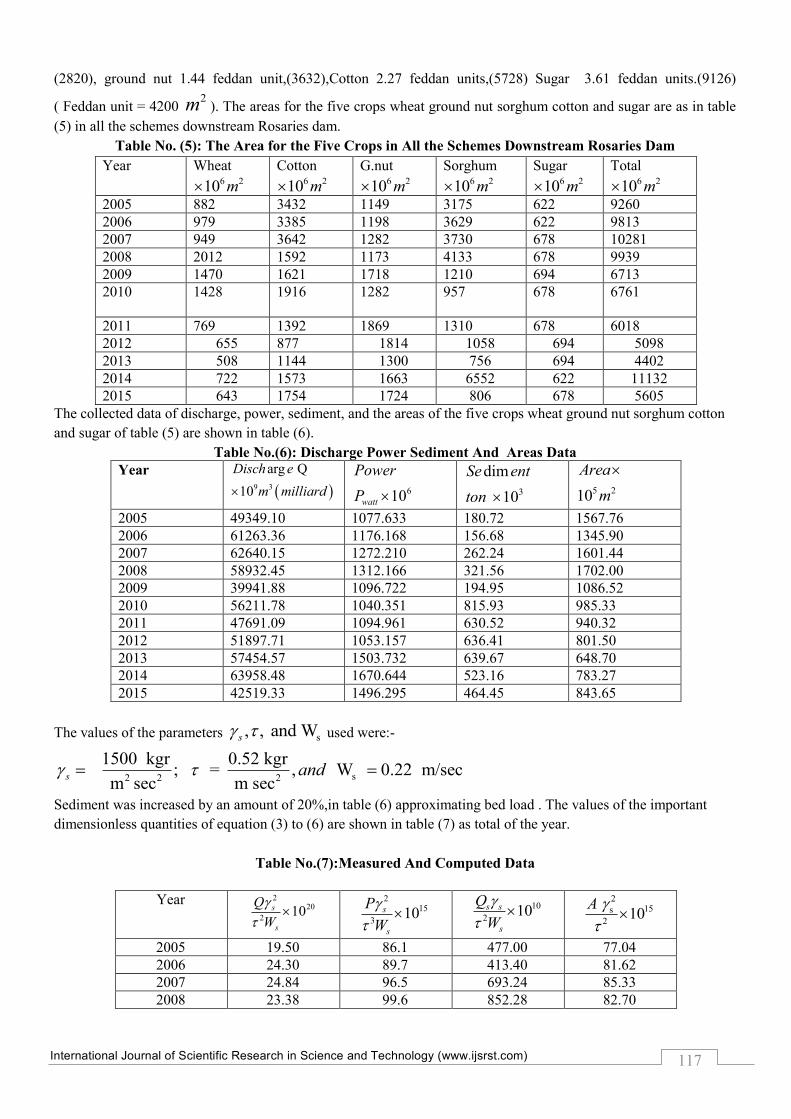
(2820), ground nut 1.44 feddan unit,(3632),Cotton 2.27 feddan units,(5728) Sugar 3.61 feddan units.(9126)

( Feddan unit = 4200 2m ). The areas for the five crops wheat ground nut sorghum cotton and sugar are as in table

(5) in all the schemes downstream Rosaries dam.

Table No. (5): The Area for the Five Crops in All the Schemes Downstream Rosaries Dam

Year Wheat 6 210 m

Cotton 6 210 m

G.nut 6 210 m

Sorghum 6 210 m

Sugar 6 210 m

Total 6 210 m

2005 882 3432 1149 3175 622 9260

2006 979 3385 1198 3629 622 9813

2007 949 3642 1282 3730 678 10281

2008 2012 1592 1173 4133 678 9939

2009 1470 1621 1718 1210 694 6713

2010 1428 1916 1282 957 678 6761

2011 769 1392 1869 1310 678 6018

2012 655 877 1814 1058 694 5098

2013 508 1144 1300 756 694 4402

2014 722 1573 1663 6552 622 11132

2015 643 1754 1724 806 678 5605

The collected data of discharge, power, sediment, and the areas of the five crops wheat ground nut sorghum cotton

and sugar of table (5) are shown in table (6).

Table No.(6): Discharge Power Sediment And Areas Data

Year

9 3

arg Q

10

Disch e

m milliard

610watt

Power

P

3

dim

10

Se ent

ton

5 210

Area

m

2005 49349.10 1077.633 180.72 1567.76

2006 61263.36 1176.168 156.68 1345.90

2007 62640.15 1272.210 262.24 1601.44

2008 58932.45 1312.166 321.56 1702.00

2009 39941.88 1096.722 194.95 1086.52

2010 56211.78 1040.351 815.93 985.33

2011 47691.09 1094.961 630.52 940.32

2012 51897.71 1053.157 636.41 801.50

2013 57454.57 1503.732 639.67 648.70

2014 63958.48 1670.644 523.16 783.27

2015 42519.33 1496.295 464.45 843.65

The values of the parameters s, , and Ws used were:-

s 2 2 2

1500 kgr 0.52 kgr ; = , W 0.22 m/sec

m sec m secs and

Sediment was increased by an amount of 20%,in table (6) approximating bed load . The values of the important

dimensionless quantities of equation (3) to (6) are shown in table (7) as total of the year.

Table No.(7):Measured And Computed Data

Year 220

210s

s

Q

W

215

310s

s

P

W

10

210s s

s

Q

W

215s

2

10

A

2005 19.50 86.1 477.00 77.04

2006 24.30 89.7 413.40 81.62

2007 24.84 96.5 693.24 85.33

2008 23.38 99.6 852.28 82.70


118

2009 15.85 92.9 515.16 55.83

2010 22.31 79.1 2162.40 56.24

2011 18.92 82.9 1669.56 50.09

2012 20.60 79.8 1685.40 42.43

2013 22.80 114.0 1695.00 36.61

2014 25.38 126.9 1386.48 92.60

2015 16.87 114.0 1230.72 46.68

To reveal the relationship among 2

2

s

s

Q

W

,and each of the dimensionless groups on the right hand side of equation (3),

simple regression analysis could be conducted. The operation can be generated by taking 2

2

s

s

Q

W

,as the dependent

variable with one group of the right hand side of equation (3),as the independent variable in each operation. The

other relations were determined in a similar way.

The multiple regression analysis is conducted using a computer program Statistical Package for Social Sciences

(SPSS) Model.The relevant dependent and independent dimensionless groups are arranged and fed to the computer.

The transformed linear relationship among the dependent dimensionless group2

2

s

s

Q

W

and independent dimensionless

groups 2 2

s

3 2 2

, ,s s s

s s

P Q A

W W

, are revealed in the form of transformed regression equations. Each transformed model

equation is expressed in the form of equation

0 1 1 2 2 3 3 y =Log a x x x 9Log a Log a Log a Log

Where:-

= y Dependent variable taken as 2

2

s

s

Q

W

0a Constant coefficient

1 2 3x x x = Independent variables taken as 2 2

s

3 2 2

, ,s s s

s s

P Q A

W W

1 2 3a a a = Exponent coefficients of 1 2 3 x x x respectively.

The output of the transformed linear regression gives the correlation r ,the constant 0a and the exponential

coefficients 1 2 3a a a with their standard error .Statistical test results namely Student ,t Test to the coefficients and

excellence of fit F – value are also given by the computer. The model regression equations accepted are those which

produce 95 % confidence level having a correlation coefficient close to (± 1),with F – Value and Student t values

greater than the tables values.

It is also very important before the application of multiple regressions on this equation to verify that the researcher

developed equations are dimensionless. The verification is carried out by the substitution of the dimensional terms

units to each supposed or obtained dimensionless groups as follows:- 2 3 2 2 4 2 5 5

2 4 4 2 2 5 5

L . . . . M . . = . .

T.L . . . . M . .

s

s

Q M L T T L TO K

W T M T L L T


119

2 2 2 3 6 3 5 7

3 3 4 4 3 3 5 7

M.L . . . M . . = O.K.

. . . . M . .

s

s

P M L T T L T

W T L T M L L T

2 4 2 3 5

2 3 2 2 2 2 3 5

M.L.M.L . . M . . = = O.K.

T . . . . M . .

s s

s

Q T T L T

W L T M L L T

2 2 2 2 4 2 4 4

s

2 4 4 2 2 4 4

L . . . M . . = = O.K.

. . M . .

A M L T L T

L T M L T

Thus the four groups are dimensionless.

The substitution of the values of the quantities is shown in table (4.6).

Referring to tables (5),of the areas of the crops,and (6) of the dimensionless groups verified above and table (2) of

all the other dimensional Parameters the results obtained are presented in the

Graphs in figures (4) to (7),containing tables, equations and charts.

Discharge Regression

Variables Entered/Removed

Model Variables

Entered

Variables

Removed

Method

1 logD, logx,

logZ . Enter

Model Summary

Model R R Square Adjusted R

Square

Std. Error of

the Estimate

1 .679 .461 .230 .06036

ANOVA

Model Sum of

Squares

df Mean Square F Sig.

1

Regression .022 3 .007 1.997 .203

Residual .026 7 .004

Total .047 10

Coefficients

Model Unstandardized Coefficients Standardized

Coefficients

t Sig.

B Std. Error Beta

1

(Constant) .060 .684 .088 .932

logx .063 .285 .063 .222 .830

logZ .144 .092 .537 1.568 .161

logD .395 .170 .803 2.329 .053


120

Residuals Statistics

Minimum Maximum Mean Std. Deviation N

Predicted Value 1.2655 1.4229 1.3244 .04672 11

Residual -.06780- .08470 .00000 .05050 11

Std. Predicted Value -1.260- 2.107 .000 1.000 11

Std. Residual -1.123- 1.403 .000 .837 11

0.063 0.144 0.3952 2 2

20 15 10 15

2 3 2 210 1.14815 10 10 10s s s s s

s s s

Q P Q A

W W W

2 2 220 15 10 15

2 3 2 210 0.06 0.063log 10 0.144log 10 0.395log 10s s s s s

s s s

Q P Q ALog

W W W

2

20

2

220 1.31389

2

10 0.06 0.063 1.94 0.144 2.68 0.395 1.89 1.31389

10 10 20.60

s

s

s

s

QLog

W

Q

W

Chart

Fig.No.(3):Relationship Among Discharge power

Sediment and Culivated Areas

Power Generation Regression


Model Variables

Entered

Variables

Removed

Method

1 logD, logy,

logZ . Enter


121

Model Summary


Square

Std. Error of

the Estimate

1 .220 .048 -.360- .07984

ANOVA

Model Sum of Squares df Mean Square F Sig.

1

Regression .002 3 .001 .118 .947


Total .047 10

Coefficients


Coefficients

t Sig.

B Std. Error Beta

1

(Constant) 1.599 .673 2.374 .049

logy .111 .498 .111 .222 .830

logZ .035 .141 .130 .248 .811

logD .072 .298 .148 .243 .815

0.111 0.035 0.072

2 2 215 20 10 15

3 2 2 210 39.7192 10 10 10s s s s s

s s s

P Q Q A

W W W

2 2 215 20 10 15

3 2 2 210 1.599 0.111 10 0.035log 10 0.072log 10s s s s s

s s s

P Q Q ALog og

W W W

2

15

3

215 1.971785557

3

10 1.599 0.111 19.50 0.035log 477.00 0.072log 77.04 1.971785557

10 10 93.71

s

s

s

s

PLog og

W

PLog

W



Predicted Value 1.9526 2.0062 1.9795 .01503 11

Residual -.09283- .09730 .00000 .06680 11


Std. Residual -1.163- 1.219 .000 .837 11


122

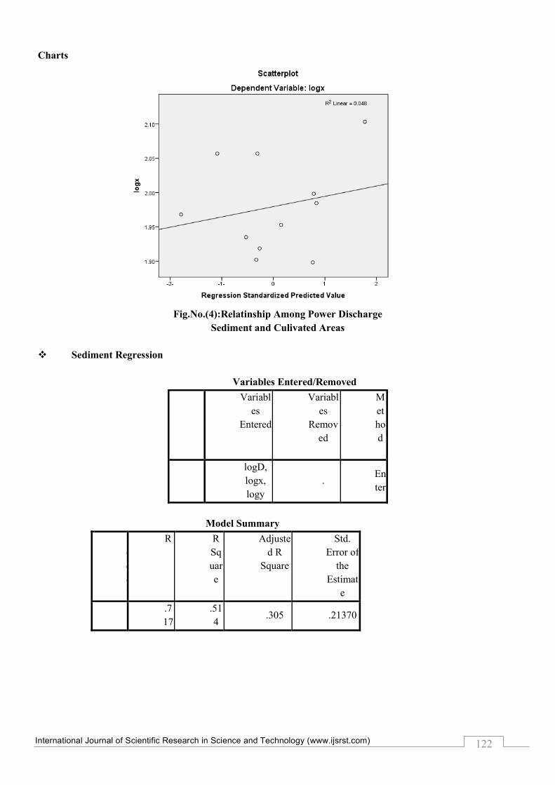
Charts

Fig.No.(4):Relatinship Among Power Discharge

Sediment and Culivated Areas

Sediment Regression


M

o

d

e

l

Variabl

es

Entered

Variabl

es

Remov

ed

M

et

ho

d

1

logD,

logx,

logy

. En

ter

Model Summary

M

o

d

e

l

R R

Sq

uar

e

Adjuste

d R

Square

Std.

Error of

the

Estimat

e

1 .7

17

.51

4 .305 .21370


123

ANOVA

Model Sum of

Squares

df Mean

Square

F Si

g.

1

Regr

essio

n

.338 3 .113

2.

46

6

.1

47

Resid

ual .320 7 .046

Total .658 10

Coefficients

Model Unstandardized

Coefficients

Standar

dized

Coeffic

ients

t Si

g.

B Std.

Error

Beta

1

(Co

nsta

nt)

2.821 2.174

1.

29

7

.2

36

logy 1.805 1.151 .484

1.

56

8

.1

61

logx .250 1.007 .067 .2

48

.8

11

log

D

-

1.512- .560 -.824-

-

2.

69

8-

.0

31


Mi

ni

mu

m

Ma

xi

mu

m

M

ea

n

Std.

Deviati

on

N

Predicted

Value

2.7

80

2

3.4

216

3.

00

22

.18380 11


124

Residual

-

.30

28

5-

.25

183

.0

00

00

.17879 11

Std.

Predicted

Value

-

1.2

08-

2.2

82

.0

00 1.000 11

Std. Residual

-

1.4

17-

1.1

78

.0

00 .837 11

1.805 0.250 1.5122 2 2

10 20 15 15

2 2 3 210 662.265 10 10 10s s s s s

s s s

Q Q P A

W W W

2 2 210 20 15 15

2 2 3 210 2.821 1.805log 10 0.250log 10 1.512log 10s s s s s

s s s

Q Q P ALog

W W W

10

2

10 2.780548255

2

10 2.821 1.805log 19.50 0.250log 86.1 1.512log 77.04 2.780548255

10 10 603.32

s s

s

s s

s

QLog

W

Q

W

Charts

Fig.No.(5):Relationship Among Sediment Discharge

Power and Culivated Areas


125

Agricultural Areas Regression


Model Variables

Entered

Variables

Removed

Method

1 logw, logx,

logy . Enter

Model Summary


Square

Std. Error of

the Estimate

1 .797 .635 .478 .10093

ANOVA

Model Sum of Squares df Mean Square F Sig.

1

Regression .124 3 .041 4.058 .058


Total .195 10

Coefficients


Coefficients

t Sig.

B Std. Error Beta

1

(Constant) 1.108 1.064 1.041 .332

logy 1.105 .474 .544 2.329 .053

logx .116 .476 .057 .243 .815

logw -.337- .125 -.619- -2.698- .031



Predicted Value 1.6544 1.9829 1.7883 .11136 11

Residual -.19410- .12266 .00000 .08445 11


Std. Residual -1.923- 1.215 .000 .837 11

1.105 0.116 0.3372 2 2

15 20 15 10

2 2 3 210 12.0781 10 10 10s s s s s

s s s

A Q P Q

W W W

2 2 215 20 15 10

2 2 3 210 1.108 1.105log 10 0.116log 10 0.337log 10s s s s s

s s s

A Q P QLog

W W W


126

2

15

2

215 1.8552879

2

10 1.108 1.105log 19.50 0.116log 86.10 0.337log 477.00

10 =10 71.66

s

s

ALog

A

Charts

Fig.No.(6): Relationship Among Cultivated Areas

Discharge Power and Sediment

III. RESULTS AND DISCUSSION

The relevant data similar to that in table (7), is not

available because no previous investigators have

conducted similar investigations. Most of the previous

investigators have conducted experimental works about

discharge sediment and power generation. No

investigator has conducted work about cultivated areas

of the different crops in the different schemes. Those

who have conducted studies about discharge sediment

and power generation, obtained quantitative and

qualitative results of certain and specific areas that can

not be applied in this study.

Although the previous investigators have covered

important studies yet it was selective and not covering

the parts studied by the researcher. However it was all

covered in the literature review so that the study would

not be incomplete. The procedures adopted by the

researcher mainly rely on basic and advanced

knowledge about dimensional analysis and theory of

models backed with SPSS supported by the advancing

knowledge of the computer analysis. Consequently, it is

very difficult if not impossible to apply the developed

empirical equations (3) to (6) to any of the previous

investigators. Equations (3) to (6) are, therefore applied

to the data taken from Rosaries Dam.

In the present study, the Cultivated Area Aspects

Relations with the other aspects was considered. The

results to the three dimensionless groups developed by

the researcher are shown in tables (8), (9),,and

(10),respectively.

Table No. (8):Cultivated Area Aspects Relations 2

15s

2

10

A

Year Predicted Actual Error

2005 71.49407 77.04 -5.54593


127

2006 96.13466 81.62 14.51466

2007 83.4411 85.33 -1.8889

2008 73.05669 82.7 -9.64331

2009 55.89462 55.83 0.064619

2010 49.34464 56.24 -6.89536

2011 45.12321 50.09 -4.96679

2012 49.19489 42.43 6.764891

2013 57.24005 36.61 20.63005

2014 69.8152 92.6 -22.7848

2015 45.71303 46.68 -0.96697

Tables No. (9): Discharge Aspects Relations 2

20

210s

s

Q

W


2005 20.58046 19.5 1.08046

2006 20.67918 24.3 -3.62082

2007 22.77655 24.84 -2.06345

2008 23.22182 23.38 -0.15818

2009 18.41228 15.85 2.562285

2010 22.47368 22.31 0.163676

2011 20.7451 18.92 1.825103

2012 19.40853 20.6 -1.19147

2013 18.74121 22.8 -4.05879

2014 26.44571 25.38 1.065714

2015 19.69994 16.87 2.829941

Table No.(10):Sediment Aspects Relations

10

210s s

s

Q

W


2005 502.3195 397.5 104.8195

2006 691.8788 344.5 347.3788

2007 685.4882 577.7 107.7882

2008 649.3667 710.2 -60.8333

2009 572.9939 429.3 143.6939

2010 1009.09 1802 -792.91

2011 903.2958 1391.3 -488.004

2012 1340.726 1404.5 -63.7741

2013 2199.936 1412.5 787.4358

2014 674.3261 1155.4 -481.074

2015 884.5655 1025.6 -141.034

IV. CONCLUSION

1. Depletion has been reported worldwide in drought

prone areas. In the Sudan, yearly losses attained the

range from 0.3% to 1.67%.

2. Although Sudan irrigated agriculture produces about

50 % of the total crop production,yet it is associated

with painstaking of removing sediments from the

irrigation network system and reservoirs.

3. Based on the results obtained in this research, it

could be admitted that Roseires Reservoir lost a

great part of its capacity due to the sedimentation

problems.

4. Data from 2005 to 20015 was used to calibrate the

hydrodynamic and morphodynamic model of the

Roseires Reservoir, and the calibration results

showed good agreements to observed data.

V. RECOMMENDATIONS

1. Complexity in reservoir operation and maintenance

coupled with downstream the dam river bank

erosion, sediment deposition, insufficient irrigation

water for the agricultural schemes, with problems in

power generation; require urgent mitigation.

2. The assessment of the impact of sediment on

irrigation water and optimization of use and

consumption of water for irrigation suggested in this

research are recommended.

3. Further research is required to evaluate the extend of

direct and indirect impact of sedimentation on

existing reservoirs where real data are available.

This will bring about the understanding, through

case studies.

4. Further research is required using modern

sophisticated model to investigate the Reservoir

sedimentation problems.


128

5. Dams and reservoirs data about soil, shear, and

water depth. are essential tools used in reseach.It is

therefore highly recommended to establish a data

base recoding all relevant research parameters.

VI. REFERENCES

[1]. Adam, A. M., (1997), “Irrigation Funding Issues

in Agricultural Schemes,” (in Arabic), A Seminar

on irrigation problems in the irrigated sector,

Khartoum, Sudan, June, 1997

[2]. Bechteler, W. (1997) "The Effects of Inaccurate

Input Parameters on Deposition of Suspended

Sediment." International Journal of Sediment

Research, 12(3), 191- 198

[3]. Dams Implementation Unit, 2012, Sudan.

[4]. FAO (Food and Agriculture Organization of the

United Nations). 1995. Assistance to land use

planning in Ethiopia (geomorphology and soils).

FAO, Rome.

[5]. Mahmood, k, (1987) reservoir sedimentation

impact.

[6]. Tan. Soon-Keat, Guoliang. Ya, Siow.-Yong. Lim

Flow structure and sediment motion around

submerged vanes in open channel Journal of the

Hydraulics Division, ASCE, 131 (3) (2005), pp.

132–136.

irrigated areas discharge and sediment interaction case ...ijsrst.com/paper/942.pdf · sudan 2civil...

Documents