The Nottingham Trent University

The Department of Computing

Shortest Path Algorithms for Public Transport

Ireneusz Szcześniak

April 2000

(Socrates/Erasmus Exchange Programme)

1

The Final Year Project has been carried out in parallel with two other Final Year Projects

which all together form a group project. The group project has been supervised by Dr

Joanna Hartley and undertaken by three Polish Socrates Exchange students from the

Silesian Institute of Technology in Gliwice, Poland. The other two students are Andrzej

Łączny (2000) and Adam Szarowicz (2000).

Acknowledgements

I would like to thank my mentor Dr Joanna Hartley for her constant encouragement and

stimulating advice. Without her help the project would not have come to its present state.

I also would like to thank Prof. Andrzej Bargiela for providing an interesting topic for the

project and for supplying equipment. The idea of the project was inspiring and

encouraging.

I would like to thank Geographers' A-Z Map Company Limited for providing a high

quality map of the Nottingham City which have been used in the group project.

2

ABSTRACT

The report is concerned with the shortest path problem, its theoretical approach,

implementation and application. First a historical background of SP algorithms is given

and basic concepts of network analysis in connection with traffic issues are explored for

the later use. The report concentrates on two SP algorithms. The first algorithm finds

one shortest path in a network with time dependent costs of links in O(n + m) time,

where n is the number of nodes, m is the number of links in the network. The second

algorithm designed for the purpose of the group project is a combination of the first

algorithm and the Dijkstra algorithm, it also runs in O(n + m) time. Both algorithms are

presented in the context of public transport networks and implemented in C++ using

Standard Template Library. At the end of the report the author’s results are discussed

and ideas for the further work are given.

“There is no need to take these writings too

seriously: let us all relax and enjoy

discussing current issues… ;-)”

-- Wim Sweldens, (1995)

3

TABLE OF CONTENTS Acknowledgements .........................................................................................................1 Abstract............................................................................................................................2 Table of contents .............................................................................................................3 Chapter 1 – INTRODUCTION

1.1 Introduction to the group project ............................................................................ 5 1.2 Introduction to the shortest path algorithms ........................................................... 6 1.3 Introduction and definition of network concepts in connection with traffic issues 8

1.3.1 Types of networks............................................................................................ 8 1.4 A general classification of the algorithms ............................................................ 10 1.5 The input and the output to the shortest path algorithms...................................... 14 1.6 Remarks ................................................................................................................ 17

Chapter 2 - LIMITATIONS

2.1 Limitations of the existing algorithms and previous research .............................. 18 2.1 Remark.................................................................................................................. 20

Chapter 3 - NEW IDEAS

3.1 Shortest path and the environment issues ............................................................. 21 3.2 Introduction to the bus routing algorithm description .......................................... 22 3.3 The bus routing algorithm..................................................................................... 23 3.4 The model of a bus transportation network .......................................................... 26 3.5 Definitions ............................................................................................................ 27 3.6 Step description of the algorithm.......................................................................... 31 3.7 The bus routing algorithm implementation using a pseudo code ......................... 33 3.8 The combined algorithm....................................................................................... 34 3.9 Kind of shortest path in the combined algorithm ................................................. 35

Chapter 4 – SOFTWARE DEVELOPEMEN

4.1 Introduction........................................................................................................... 40 4.2 Why STL?............................................................................................................. 41 4.3 The code................................................................................................................ 42

Chapter 5 – RESULTS AND DISCUSSION

5.1 Results................................................................................................................... 44 5.1.1 Results of the bus algorithm .......................................................................... 44 5.1.1 Results of the Dijkstra algorithm................................................................... 46

5.2 Discussion............................................................................................................. 47 5.3 Performance of the bus algorithm......................................................................... 47 5.4 Performance of the Dijkstra algorithm implementation ....................................... 49 5.5 Performance of the combined algorithm............................................................... 50

Chapter 6 – CONCLUSIONS AND FUTURE WORK

5.1 Conclusions........................................................................................................... 51 5.2 Future work........................................................................................................... 52

4

References......................................................................................................................54 Appendix A....................................................................................................................56 Appendix B ....................................................................................................................62 Appendix C....................................................................................................................70 Appendix D....................................................................................................................71 Appendix E ....................................................................................................................73 Appendix F ....................................................................................................................74 Appendix G....................................................................................................................77 Appendix H....................................................................................................................79 Appendix I .....................................................................................................................82

5

Chapter 1 - INTRODUCTION

1.1 Introduction to the group project

Prof. Andrzej Bargiela has proposed the idea of the group project. All the group project

is about is to develop a program to help the user find the best way to commute from home

to work.

As this point the traffic advisor will only be a game, not a program ready for a daily use.

This is a prototype of a program to be developed in the future. Now the program works

on a fixed traffic data and on a manually processed map. In the future data is going to be

collected online from traffic sensors of the SCOOT system. The real online data will

serve for realistic control and advice.

One of the chief objectives was the low cost of the program. Therefore the whole

application has to be developed from scratch. It cannot use commercial databases to

store traffic and road data, software to present the output (as MapInfo) or software for

shortest route finding (as MS Route Finder) because of the high cost they induce. Each

part of the program had to be programmed from the basics in the C++ language.

A natural way of dividing the program among three programmers is to split it up into

three main modules: the graphic user interface module, the database module and the

shortest path algorithm module. Adam Szarowicz has written the database module

6

(2000). Andrzej Łaczny has prepared the graphic user interface module (2000). The

author’s part was the shortest path algorithm module.

1.2 Introduction to the shortest path algorithms

The shortest path (SP) algorithms are among fundamental network analysis problems.

Since 1957 a considerable progress has been made in the SP algorithms after Minty

published his paper (1957). Minty succinctly described the basic SP problem for

symmetrical networks (a network is symmetrical if for every pair of nodes the cost of a

link between the two nodes is independent of the starting node). To state the problem

beyond doubt, he suggested constructing a model of the given network. The model is

made of strings, each string of the length proportional to the costs of the modelled link.

Finally, to find the links of the SP one has to pull the source node and the destination

node of the journey as far away as possible. The tight strings are the links of the SP.

Since 1957 there has been a number of major papers published, the most important were

published by Bellman (1959), Dijkstra (1959) and Moore (1959). These articles were

formative and most of the traffic research has used their results (for example Clercq

(1972) or Cooke and Halsey (1966)). These articles are now included in references by

most other publications.

There is a number of review papers. One of the utmost importance has been published by

Dreyfus (1969). The review gives a comprehensive summary of the research which has

7

been carried out up to 1969. The article surveys over ten years of research, discussing

the most crucial stages and pointing out the wrong and inefficient solutions. The more

important, the paper gives briefly a solution of the SP problem for time varying costs of

links, which is the basis of this report.

The shortest path algorithms are currently widely used. They are the basis of the network

flow problems, tree problems and many related other problems. They determine the

smallest cost of travel, of a production cycle, the shortest path in an electric circuit or the

most reliable path. In the book by Ahuja at al. (1993) one can realise that the SP problem

is an underlying problem of the network optimisation and that it is closely related to

network flows or tree building issues.

Internet is a large filed where the shortest path algorithms ca be applied. The Internet

problems involve data packages transmission with the minimal time or by the most

reliable path. An example of the SP algorithms in the Internet is given by Cai et al.

(1997). This paper proposes three SP algorithms. The devised algorithms are well

explained. The article is closely related to our problem. The same algorithms can be

used without fundamental changes to the urban traffic issues. The use of the proposed

algorithms for public transportation networks will be studied in the section ‘Shortest path

and the environment issues’.

Algorithms to be discussed here have a thirty-year old history and solutions to the

fundamental problems are well known. The contemporary research is directed toward

8

parallel computing as the method for further lowering of the time complexity bound of

the shortest path algorithms. The report is not interested in the parallel approach. The

article by Klein and Subramanian (1997) is an example of the shortest path parallel

algorithm.

1.3 Introduction and definition of network concepts in connection with traffic issues

1.3.1 Types of networks

There are several types of networks of special interest to the project: sparse, planar and

road networks. Other types of networks (as grid or dense) are not taken into account.

Sparse networks

Sparse networks are those which have the number of links only a few times bigger than

the number of nodes. A network of 100 nodes and 400 links would be considered sparse

but a network with 100 nodes and 5000 links would be classified as dense.

Public transportation networks are sparse. From each node approximately four links

leave. If a sparse network was presented in a matrix form, then in each row of the matrix

about only four places would be used, the rest would be left idle. For matrix network

representation there are algorithms which handle efficiently the sparse networks.

However, it is recommended not to use matrix-based algorithms since the matrix

9

representation of a sparse network is highly inefficient. Instead of the matrix algorithms

the tree building algorithms can be used as they store the sparse network information in a

efficient way (usually using lists). In this report the Dijkstra algorithm has been used

which is a basic tree building algorithm. The matrix in fig. 3. is an example of the

inefficient matrix representation of a sparse network since there is more places unused

than used.

Planar networks

There are a number of SP algorithms for planar graphs. Methods characteristic to planar

graphs (as separators) lower the computational bound of the SP algorithms.

Since the road network and public transport network are mostly planar, application of the

algorithms from this group could bring more efficient solutions to our problem. However,

not all road networks are planar, there are viaducts and bridges which can destroy

planarity and thus unable, limit or complicate the application of these algorithms.

Because of this reason the methods for the planar graphs will not be considered. The

article by Monika R. Henzinger et al. (1997) proposes three new algorithms for planar

graphs.

10

Road networks

In the representation of a road network a link represents a road and a node represents a

crossroad. The ratio of the number of links to the number of nodes is approximately 3.

(Steenbrink, chapter 7, page 150, gives an example of a road network with about 2000

nodes and 6000 links). The link costs are always non-negative. The rood networks are

usually planar and sparse. The number of nodes is big, usually expressed in thousands.

Road networks contain loops which are allowed since they may be only of a non-negative

cost (the link costs are only non-negative). The road networks are of a special interest in

this report.

The characteristic feature of the road networks is their always nonnegative link lengths

property. Dijkstra made a good use of nonnegative lengths to design his algorithm.

Because of this close relation between Dijkstra algorithm and road characteristic, it

should not be surprising that this report suffers constant ‘Dijkstra’ referring.

The project’s road network of the Nottingham City had 218 nodes and 787 links. The

network represents the link connections between nodes and the distances between them.

1.4 A general classification of the algorithms

The SP algorithms are either matrix algorithms or tree building algorithms (tree

algorithms are also called labelling algorithms).

11

Matrix algorithms

Matrix algorithms store the network information in the matrix form and carry out the

computations using basic matrix operations (as addition and multiplication of matrices or

matrix’s elements). For dense networks and for all pair problem.

The disadvantage of the matrix algorithms is the imposed matrix representation. The first

disadvantage is the imposed inefficient matrix representation of a sparse network. The

more significant disadvantage is that the matrix representation allows one directed link

between two nodes (there can be at most two links between two nodes, but they have to

be of distinct directions).

1

5

6

2 4

3

1

1

1

1

31

3

2

1

2

Fig. 1. A sample network that can be represented in a matrix form.

12

1

5

6

2 4

3

1

1

1

1

1

3

2

1

3

24

Fig. 2. A sample network that can be not represented in a matrix form.

∞∞∞∞∞∞∞∞∞

∞∞∞∞∞∞∞∞∞∞∞

=

010110

1103320

210

M

Fig. 3. Matrix representation of the network from fig. 1.

The network from fig. 1. is specified by a matrix in fig. 3. Not every network can be

represented in such a way. If a network has more than one directed link from a single

node to some other node, then it cannot be represented in a regular matrix since it can

store only one directed link going from a specific link to some other node.

A sample network capable of being represented as a matrix is depicted in fig. 1. The

network has two links connecting the 1st node to the 3rd node. The link from the 1st node

to the 3rd node is ascribed the cost of 2, which is stored in the M matrix in fig. 1. as

a13 = 2. The link which goes in the reverse direction (from the 3rd node to the 1st node) is

ascribed the cost of 3, this is stored as a31=3.

13

If there was a need to represent the three links between the 1st and 3rd nodes from the fig.

1. then we realise we have run out of places in the matrix and the network cannot be fully

represented by a matrix.

There can be some improvements of the matrix representation envisaged for coping with

such an extended network. One improvement is a matrix of lists. An entry in this matrix

of lists would not characterise only one directed link from one node to another but a list

of directed links from this node to another node. However, this is not classified anymore

as the matrix approach to the SP problem because computations of most matrix

algorithms would not be performed anymore using basic matrix operations.

The tree building algorithms

The project’s algorithms are tree building algorithms. A tree building algorithm builds a

tree with the root in the source node of the trip. Each node of the network can be either a

leaf or a fork of the tree. A fork leads to another forks or leaves. There are certain true

statements about the tree. The first is that there are p leaves then these leaves are p nodes

of the biggest cost to reach among all nodes. The second says that each fork node (a node

that is a fork in the tree) is of the cost smaller than a cost of any leaf node (a node that is

a leaf in the tree).

Building such a tree is a dynamic programming task since the result of a node just

reached can be used to calculate the cost of the node which can be reached immediately

14

after this node. An example of building a tree for a simple network is presented in the

fig. 4. To build this tree we use the Dijkstra algorithm.

1

5

6

2

2

1

1 2

12

a) network

1

2 3

4

5

6

3

4

11

1

1

1

3

b) tree

1

1

cost:1

cost:3

cost:2

cost:0

cost:3

cost:4

4

Fig. 4. A network and its shortest path tree.

1.5 The input and the output to the shortest path algorithms

“Where have you been?

Where are you going to?”

— Chris Rea, The blue cafe (1998)

Depending where we are and where we want to go an algorithm can find as many SP’s as

it is necessary to satisfy us. The SP algorithms can be divided into groups that differ by

15

the given input and the desired output. The groups are: one pair algorithms, one to many,

many to one and all pairs algorithms.

one pair

There are two nodes given: the source node and the destination node. A SP algorithm

finds only one SP (if it exists) from the given source node to the given destination node.

The tree algorithms are going to build an incomplete tree with the root in the source

node. The tree will be complete up to the moment the destination node has been reached.

The Dijkstra algorithm (1959) and the Bellman (1958) algorithm are examples are one

pair algorithms.

one to many

Only the source node is specified. All shortest paths from this source node to all other

nodes will be calculated. If there is a path from the source node to every other node, then

there will be (n-1) SP’s evaluated (n is the number of nodes is the network). A tree

building algorithm will create a complete shortest path tree. The Dijkstra algorithm and

the Bellman algorithm are also examples of one to many algorithms.

many to one

16

This problem is given many source nodes and one destination node. To each source node

there is time ascribed saying what time the journey starts from this node. The solution to

the problem is to find the shortest path from any source node to the destination node that

will result in reaching the destination node at the minimal time of arrival (not cost of the

journey).

This type of a problem is easy to solve having the Dijkstra algorithm. The solution

doesn’t differ significantly from the Dijkstra algorithm. Only at the beginning one has to

put all the source nodes into the priority queue with appropriate costs.

all pairs

For this algorithm group there is neither source node nor the destination node necessary.

An algorithm from this group calculates all the possible SP’s, i.e. the algorithm is to find

the shortest path for every pair of nodes. The number of paths is therefore n2-n = n(n - 1)

(the paths form one and the same node is 0 and doesn’t require calculation). The

computations are mostly done on matrices. The Floyd algorithm (1962) is an example

from the all pairs algorithm group.

One to one, one to many, many to one, all pairs and the project

The project makes use of ‘one to many’ algorithm and ‘many to one’ algorithm only. The

‘all pairs’ algorithm is not essential for the project and will not be discussed.

17

1.6 Remarks

The terms network and graph will be used interchangeably.

The terms link cost and link length will be used interchangeably though the term link cost

will be used more generally.

The terms starting node and finishing node will refer to the starting node and the

finishing node of a link. The source node and the destination node terms are going to

denote the starting node (initial node) and the finishing node (terminal node or sink) of

the overall shortest path, respectively.

18

Chapter 2 - LIMITATIONS

2.1 Limitations of the existing algorithms and previous research

Among several variants of the SP algorithms there is a group of algorithms which could

be applied to solve the present issue, but the solution would not be efficient. An obvious

group of algorithms is the one that gives a more general solution than needed and their

solution would be redundant. A good example of a group giving a redundant solution is

the ‘all pairs’ group of the SP algorithms: only one pair of nodes would be used from the

set of all pairs.

Matrix algorithms are not of a good use for sparse networks. Matrix algorithms are

memory consuming and for sparse networks time consuming. The implementation of the

Dijkstra algorithm based on a matrix is inefficient for road networks. Therefore the

matrix algorithms are abandoned from this point for the rest of the report.

Bellman (1958) designed an algorithm for networks with also negative link lengths. The

concern about negative link length made the Bellman algorithm more general than

Dijkstra algorithm, but it also made it less efficient for the networks without negative

links. Since the report deals with road networks (of which the inherent feature is the

nonnegative link lengths) only, the study of the Bellman algorithm will not be of much

interest for the report.

19

Another example of an algorithm providing a solution more general than needed is the

algorithm devised by Cai et al (1997). This algorithm is an enhanced Dijkstra algorithm.

The algorithm processes a network to whose links two attributes are ascribed: cost of

traversing and time of traversing. The algorithm searches for the cheapest path (the

shortest path in terms of the cost) which satisfies an extra condition: the overall time of

such a path (the time required to traverse the links of the path) does not exceed a given T.

The algorithm can be used to solve the project’s problem by setting every link’s time to 0

and setting T = 0. Such a solution is not efficient thought.

An algorithm by Cooke and Halsey (1966) finds the shortest path from one source to one

destination in a network with time dependent link costs. The algorithm is based on the

Bellman approach (the paper was also submitted by Bellman). The algorithm works out

but unfortunately is inefficient. The description of the algorithm is complicated and not

clear. The algorithm was revised by Dreyfus (1969) who pointed out the inefficiency of

the algorithm and proposed his solution to the problem.

F. le Clercq published his paper in 1972 in which he proposed an algorithm for public

transport. The algorithm does not use timetables which is the main requirement for the

group project, the algorithm proposed by F. le Clercq uses frequencies of bus lines

instead. The algorithm is vaguely described without emphasis of main ideas and firm

specification of the algorithm. The paper does not report the time complexity and

memory requirements.

20

2.2 Remark

The author of this report encountered (mostly in the book by Streenbrink (1974) and in

the article by F. le Clercq (1972)) references to public transport papers written in

languages (mostly Dutch) which the author of this report does not speak. Because of this

reason many potentially useful sources have not been reached and cannot be discussed.

21

Chapter 3 - NEW IDEAS

3.1 Shortest path and the environment issues

Suppose there is a need to find a path which implies the smallest usage of fuel. This case

is similar as the money cost of the travel, but it differs since the bus money cost (the

money for a bus ticket, for example) is higher than (and not linear to) the fuel used. The

shortest path in terms of used fuel needs to be evaluated from the environment point of

view.

The simplest approach to the problem is to ascribe a cost to every link costs that

expresses the impact on the environment. Therefore a higher cost will be attached to a

car link, and a smaller cost will be attached to the bus link. The cost of a link should be

dependent on the length of this link. According to the criteria of cost, the algorithm

searches for the shortest path and at the same time computes the time cost.

The time cost of a shortest path generated with the help of such an algorithm will not be

optimised. We can conceive the case where there is the shortest path found in terms of

the lowest fuel cost, but the time cost is not acceptable. This may happen is we waited a

long time to save not a significant amount of fuel.

A number of constraining criteria for such a shortest route finding can be given. First, we

can fix a certain amount of time which can be taken at most for waiting at a bus stop.

22

Among the links that fulfil this condition, the link of the smallest fuel cost is chosen.

Another constraint can be that the overall travel time cannot be greater than a fixed

amount T.

In the article by Cai at el.(1997) one can find three algorithms for the internet data

packages routing among which one algorithm is very well suited to our needs. The

algorithm searches a specific type of networks. Each link in the network has two numbers

ascribed: cost and time. For us the cost can be the fuel cost and time is the time cost.

The proposed algorithm is going to find the shortest route according to fuel cost and with

the overall time cost not exceeding a specific amount of time T.

The main ideas of the project are involved in the adaptation of the algorithm proposed by

S. D. Dreyfus (1969) for bus networks which is based on the Dijkstra algorithm.

The main ideas have been used to adopt the algorithm described by Dreyfus (1969) to the

public transportation networks, to describe it mathematically.

3.2 Introduction to the bus routing algorithm description

The algorithm can be used to any public transportation network based on timetables.

Since a bus is a public transport mean the project takes into account, the algorithm for the

public transport mean based on timetables is called in the report the bus routing algorithm

23

3.3 The bus routing algorithm

To understand the problem clearly, it is useful to visualise a user who wants to get from

one bus stop to another in a city using buses only. The input data to the algorithm

consists of a description of the bus transportation network (timetables, description of

connections between bus stops), the bus stop where the journey begins (the source node)

and the bus stop at which the journey ends (the destination node). The objective is to find

the shortest path between the two specified nodes, namely the path that requires the

minimal amount of time.

The algorithm presented here was designed to solve the problem described in short

above. The new algorithm had to be designed in order to meet the special needs of bus

transportation networks such as timetables and the possibility of waiting at bus stops. The

chief difference between the standard shortest path problem and this one is that links vary

with time and that it is allowed to wait at the nodes as long as it is necessary to obtain the

minimal time cost. The problem can be classified as the shortest path problem with time

dependent costs of links and the allowance of waiting at nodes. A time cost of every link

may differ in any desired way.

The solution to the problem is based on the Dijkstra algorithm which is the best known

algorithm for directed networks with nonnegative link costs. There are several principles

(as the use of a priority queue or the use of buckets) underlying an efficient

24

implementation of the Dijkstra algorithm which can also be applied to implement the bus

algorithm (the article by Cherkassky at al is a good paper discussing principles for

Dijkstra algorithm implementation).

The Dijkstra algorithm has to be modified because of two problems.

The first modification deals with a problem of fixed times at which a bus leaves a bus

stop. This new attribute of a link is going to be named the departure time of a link. The

Dijkstra algorithm is not concerned with a departure time of a link; the algorithm was

designed to work with links which can be used at any time. In our problem the main

constraint is that links cannot be used at any time, the time at which a bus link can be

used is fixed according to a timetable.

The second problem is the actual cost of a bus connection between two nodes. In our case

the cost of a link is not the criterion to judge the optimality of the link choice anymore. In

the present problem the actual criterion is the sum of the waiting time and the link cost,

or, in other words, the time of arrival at the finishing node of a link. In effect, we are also

concerned with the waiting times at nodes. The need to wait at bus stops is a consequence

of the departure time attribute (if a link cannot be used right now then it is necessary to

wait for the departure).

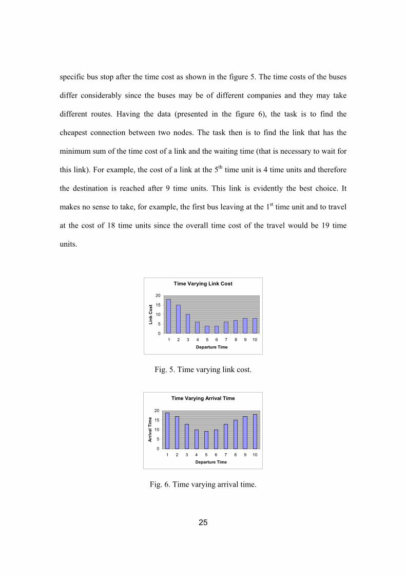
The figures 5 and 6 depict the problem of the overall cost of a link. Suppose there are

buses leaving a specific bus stop at 1, 2, …, 10 time units and arriving at the other

25

specific bus stop after the time cost as shown in the figure 5. The time costs of the buses

differ considerably since the buses may be of different companies and they may take

different routes. Having the data (presented in the figure 6), the task is to find the

cheapest connection between two nodes. The task then is to find the link that has the

minimum sum of the time cost of a link and the waiting time (that is necessary to wait for

this link). For example, the cost of a link at the 5th time unit is 4 time units and therefore

the destination is reached after 9 time units. This link is evidently the best choice. It

makes no sense to take, for example, the first bus leaving at the 1st time unit and to travel

at the cost of 18 time units since the overall time cost of the travel would be 19 time

units.

Time Varying Link Cost

0

5

10

15

20

1 2 3 4 5 6 7 8 9 10

Departure Time

Link

Cos

t

Fig. 5. Time varying link cost.

Time Varying Arrival Time

0

5

10

15

20

1 2 3 4 5 6 7 8 9 10Departure Time

Arr

ival

Tim

e

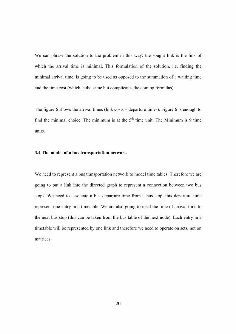
Fig. 6. Time varying arrival time.

26

We can phrase the solution to the problem in this way: the sought link is the link of

which the arrival time is minimal. This formulation of the solution, i.e. finding the

minimal arrival time, is going to be used as opposed to the summation of a waiting time

and the time cost (which is the same but complicates the coming formulas).

The figure 6 shows the arrival times (link costs + departure times). Figure 6 is enough to

find the minimal choice. The minimum is at the 5th time unit. The Minimum is 9 time

units.

3.4 The model of a bus transportation network

We need to represent a bus transportation network to model time tables. Therefore we are

going to put a link into the directed graph to represent a connection between two bus

stops. We need to associate a bus departure time from a bus stop, this departure time

represent one entry in a timetable. We are also going to need the time of arrival time to

the next bus stop (this can be taken from the bus table of the next node). Each entry in a

timetable will be represented by one link and therefore we need to operate on sets, not on

matrices.

27

Table 1. A bus connection between the City Centre and Clifton.

City Centre Arriving to Clifton 7:10am 7:30am

12:35pm 13:00pm 17:20pm 17:50pm 22:50pm 23:05pm

Table 2. is a table with a subset of links that represent a bus connection described by the

timetable of table 1.

Table 2. Representation of a bus connection from the table 1 in the form of links.

Starting node Finishing node Departure time Arrival time City Centre bus stop Clifton bus stop 7:10am 7:30am City Centre bus stop Clifton bus stop 12:35pm 13:00pm City Centre bus stop Clifton bus stop 17:20pm 17:50pm City Centre bus stop Clifton bus stop 22:50pm 23:05pm

3.5 Definitions

We introduce new definitions and concepts to model the bus network conveniently and to

describe the algorithm precisely.

28

Definition of the network

We are given a directed graph G(V, E ,d ,a), V is the set of nodes (Vertices) and E is the

set of links (Edges). We denote the number of element of the set V of nodes as n = |V|

and the number of links of the set of E as m = |E|. We will refer to a node of a graph by

‘xj‘ and to a link by ‘e’. Function d : E α R∪ {∞} (the infinity can be ascribed to a link,

therefore it is included) associates with every link a departure time (a real nonnegative

number) from the staring node and the function a : E α R∪ {∞} ascribes the time of

arrival (a real nonnegative number) at the finishing node. The departure time d(xj) of the

xj link (from the staring node) is the time at which the link may be used, it cannot be in

use at any other time. The arrival time a(xj) of the xj link is the time at which we get to the

finishing node of the link.

If it is necessary to know the time cost of the xj link (time required to traverse the link),

we can calculate it in this way: c(xj) = a(xj) - d(xj). We can describe uniquely a link of the

graph only by four numbers (xi, xi+1, d(xi), a(xi)) where xi is a starting node of the link, xi+1

is the finishing node of the link, d(xi) is the departure time and a(xi) is the arrival time.

Referring to a specific link only by a pair (xi, xi+1) can be ambiguous since there can be

two or more links between the xi and xi+1 nodes, links may differ in the departure time or

the arrival time.

29

The Symbol

The symbol X represents a powerset of a X set (i.e. the set of all subsets of the X set).

Definition of the slbtn function

slbtn : V×V α E

Set of Links Between Two Nodes

The slbtn function takes a pair of nodes (xi, xi+1) and returns the set which comprises

every link that starts at xi node and finishes at the xi+1 node.

Definition of the slcsn function

slcsn: V α E

Set of Links of Common Starting Node

The function returns all the links that have the node given as the argument as the starting

node.

Definition of the arrival time at a specific node

T(xi) is the time of arrival at the node xi. Let t0 be the time at which the journey starts.

We define T(xi) recursively.

30

)()}()(|),({

min)(

)(

1

1

0

eaxTedxxslbtne

xT

tsT

iii

i

≥∈=

=

+

+

Note that T(xi) is not the cost of the shortest path. It represents the time at which the node

is reached. The cost of getting to a node let’s say x17 may be only ten minutes, but

T(x17) = 17:10 if we started the journey at 17:00.

Definition of a path

Let P = (s = x1, x2, …, x = xr) be a path form the s node to the x node. The s node is the

source node of the path and the x node is the destination node of the path.

Definition of the shortest path

Let P = (s = x1, x2, …, x = xr) be the shortest path from the source node s to the

destination node x. The nodes of the shortest path are such that they result in the minimal

arrival time to the xr node. The time of arrival is given by T(xr).

The subsequent nodes of the shortest path are found by the use of T(xi) function. To find

xr-1 we have to find the link which led to xr with minimal arrival time. Having the link,

we have the starting node of the link. This starting node is the xr-1 node of the shortest

path. This method has to be repeated until the source node is reached.

31

3.6 Step description of the algorithm

The aim of the algorithm is to minimise T(x) (x is the destination node). To minimise it

we first have to minimise T(xi) for nodes xi which are at the shortest path from s to x.

Before we get to the algorithm description, there are some definitions to be introduced.

We classify all the nodes of the graph into three sets, every node can be a member of only

one of the following sets:

• SPN: the Set of Permanent Nodes is the set of nodes which have been completely

processed, the time of reaching these nodes has been computed and will not change.

• SSN: the Set of Scanned Nodes is the set of nodes which have been reached, but

have not been completely processed, the time cost of getting to them is known but

may change.

• SNRN: the Set of Not Reached Nodes is the set of nodes which have not been

reached at all.

The step description

Step 0

The source node s is initialised as scanned (s ∈ SSN) and every other node xi ≠ s of the

graph is initialised as not reached (xi ∈ SNRN). Furthermore, the arrival time of the

32

source node is set to t0 (t0 is the time at which the journey starts), i.e. T(s) = t0, and the

arrival time of every other node xi ≠ s of the graph is set to infinity, i.e. T(xi) = ∞.

Step k

We process only one node during this step. We choose the node to be processed from the

SSN (Set of Scanned Nodes). If the SSN is empty, this means there is no path between

the source node and the destination nodes and the algorithm quits. If the SSN is not

empty, we choose a xi node from the SSN which has minimal T(xi). If there is more than

one node with the minimal T(xi) then we choose one of them arbitrarily. In formula:

SSNx

xTxTSSNx

j

jii

∈

=•∈ )(min)(

Once the xi node is chosen, we proceed to process it. First the node xi is excluded from

the SSN and becomes a member of SPN (Set of Permanent Nodes). At this stage it is

certain that the arrival time T(xi) is minimal (it may only get larger since taking another

link will increase the cost; link costs are always positive) and this is the reason for

moving the xi node to SPN.

Next the links leaving the xi node are handled. From the set E (the set of links of the

graph) every link which has the xi node as a starting one is selected. The retrieved set is

further constrained to links of the departure time greater or equal to T(xi) (only buses that

will arrive to a bus stop can be taken, not those which have left). Writing it down in a

formula:

33

{ })()(|)()( edxTxsllsnex iii ≤∈=α

The empty α(xi) set denotes there are no buses leaving the xi node after T(xi) or there are

no buses at all.

The set α(xi) is divided into subsets, each subset having links of a distinct finishing xi+1

node. In consequence, all subsets have the same starting xi node and each subset has a

unique finishing xi+1 node. Therefore, for example, if it is possible to get from the xi node

to other, let’s say, 3 nodes, that means there are going to be exactly 3 subsets.

For each subset we examine if the finishing node xi+1 of the subset is in the SPN. The

statement xi+1 ∈ SPN implies that the minimal value T(xi+1) has been found and we can

proceed to process a next subset. If xi+1 ∉ SPN , we have to find in the subset a link e for

which a(e) is minimal. If it occurs that the value a(e) is smaller than T(xi) previously

found, i.e. a(e)<T(xi+1), then the new value of T(xi+1) is set T(xi+1) = a(e). At the end of

processing each subset we make sure that the xi+1 node is a member of SSN (if it is not, it

has to be moved to the SSN).

3.7 The bus routing algorithm implementation using a pseudo code

Let p_queue be a priority queue of nodes. The order of nodes xj in the queue is pointed

out by the increasing values of T(xj), so that at the beginning of the queue there is a node

which has the smallest T(xj).

34

p_queue = ∅

for every node xk∈ V set the value T(xk) = ∞

set value T(s)=to

push s into the priority queue p_queue

while(p_queue ≠ ∅ )

xi = get_first(p_queue)

for every xi+1∈ V such that (xi, xi+1) ∈ V

calculate:

)}()(|),({)(min

1 iii xTedxxslbtneeaT

≥∈=

+

if T<T(xi+1) then

if T(xi+1) = ∞ then

push xi+1 into the priority queue p_queue

T(xi+1) = T

3.8 The combined algorithm

The bus algorithm can be used as a standalone algorithm. It is complete and ready to use.

It can be used to find the shortest path in a bus transportation network and the obtained

path will only be composed of bus links.

35

However, the algorithm can be combined with other algorithms to be used for different

purposes. This section is concerned with the combination of the bus algorithm and the

Dijkstra algorithm to describe the combined algorithm.

The demand for the combined algorithm emerged from the need of the group project.

Initially the group project has been meant to make use of buses only. Gradually new

ideas came up and finally the design of an algorithm to deal with both cars and buses

became apparent.

The final definition of the combined algorithm is as follows. The algorithm is given the

road network and the public transport network (together with timetables). The algorithm

has to find the shortest route from one place to another using both a car and a mean of

public transportation. The required output has to be composed of car links and bus links.

3.9 Kinds of shortest paths in the combined algorithm

There are three methods using which the shortest path (i.e. with the optimal cost – either

with the time cost or the environment cost) can be found in the combined algorithm.

First the user may specify that the journey begins with a car. The user may want for

some reason to begin the journey with a bus – this is the second way. The third way is

that the user is interested with the most optimal path and does not determine weather to

start with a car or a bus.

36

Let’s start with a car

The user starts the journey with a car and reaches the destination either by a car or by

buses (there is unlimited number of changes between buses). The change from a car to a

bus may take place only once and only at a Park & Ride. Such rules induce two kinds of

the shortest path and the algorithm searches for the best path among these two kinds of

shortest paths. The first kind of a path is composed only of the car links, i.e. the user will

have to use only a car during the whole journey. The second type of a path is a path that

starts with a car, continues to a Park & Ride and reaches the destination with links only

buses (there is unlimited number of changes allowed between buses). Fig. 7 depicts the

two possible paths which can be found.

Park & RideSource Bus StopBus Stop Destination

car

bus buscar bus bus

bus = a sequence of bus l inks

= a sequence of car l inkscar

...

Fig. 7. Two kinds of a shortest path starting with a car.

Let’s start with a bus

The situation is analogous to starting the journey with a car. This time the user starts

with a bus and reaches the destination either by buses (there is unlimited number of

changes between buses allowed) or by a car. The change from a bus to a car may take

place only once and only at a Park & Ride. Such rules induce two kinds of the shortest

37

path and the algorithm searches for the best path among both kinds of shortest paths. The

first kind of a path is composed only of the bus links, i.e. the user will have to use only

buses during the whole journey. The second type of a path is a path that starts with a bus,

continues with unlimited number of changes between buses to a Park & Ride and reaches

the destination with car links only. Fig. 8. depicts the two possible paths which can be

found.

Park & Ride DestinationBus Stop Bus StopSource carbus bus

Bus Stop Bus Stop...bus busbusbus

bus bus

bus = a sequence of bus links

= a sequence of car linkscar

...

Fig. 8. Two kinds of a shortest path starting with a bus.

Start either with a bus or a car, just get the optimal path

In the two previous ways the user had to specify what to start with, a car or a bus. First

the user may say that any path is the best as long as it is the shortest. Therefore the user

can begin the journey with either a bus or a car. At the beginning of the journey the user

takes a car. He can reach work by car only but it may happen that using a bus he will get

to the work in a shorter time. In the morning there is a considerable amount of traffic

which makes the trip to work long. Changing to a bus may shorten the time because

buses have separate lanes.

38

There are a number of constraints concerning car to bus changes. The fundamental is that

the user can leave the car at the Park & Ride places and nowhere else. There is no

restriction to the number of bus changes. Therefore every route from home to work looks

as shown in the fig. 9.

Park & Ride

Source

Bus StopBus Stop

Destination

car

busbuscar

bus bus...

Park & RideBus Stop Bus Stop bus

Bus Stop Bus Stop... busbus

bus bus

bus = a sequence of bus links

= a sequence of car linkscar

...bus car

bus bus

Fig. 9. Every possible form of a shortest path in the combined algorithm.

On the way from home to work the user can go directly to work or can change to a bus.

The change has to be made on a Park & Ride place. After the change the user can take

any number of buses to finally reach work.

Conversely, on the way from work to home the user can take a car and make his way

straight home but he is left the choice to take any number of buses to reach the Park &

Ride place to finally get home from there.

The way the combined path algorithm for the journey from home to work calculates is

intuitive. First the shortest path algorithm for car links is run. The algorithm is called to

39

find the shortest route to work and all Park & Ride places. Next the algorithm for buses is

run for each Park & Ride place to find the shortest path from this Park & Ride place to

work. In this way we get several shortest paths: straight from home to work, and from all

Park & Ride places to work. From these paths the best path can be chosen.

In the same way the algorithm from work to home works. First the algorithm for buses is

called to find the shortest route to each Park & Ride and home. Next the shortest path

algorithm for a car is called to find the shortest paths from work to home and from work

to all Park & Rides.

40

Chapter 4 – SOFTWARE DEVELOPMENT

4.1 Introduction

The software has been developed only for the use of the group project. Therefore the

whole software has been oriented toward the application. The author has been aiming

only for a basic independence from the group project.

A careful implementation of a time consuming shortest path algorithm saves expensive

and crucial time. Not only the general principle underlying an implementation of an

algorithm should be considered meticulously (as whether to choose a priority queue or a

list), but the chosen principle should be well coded. Steenbrink (1974, chapter 7, page

153) gives an example of a four times increased performance of a SP algorithm which

has been achieved by technical changes in a program.

The author of this report also paid attention to the technical details in order to increase

the implementations’ performance. The usage of automatic objects has been restricted as

much as possible to limit stack manipulations. Loops have been reorganised for

processing more data in each step in order to lower the execution of loop organisation

code imposed by the compiler. Moreover, the number of subroutines’ arguments has

been optimised for efficient data passing.

41

The first phase of development involved writing of the basic code. This code has been

written to be project independent, i.e. to serve also other. The basic code allows is for the

network modelling. It

4.2 Why STL?

The author decided to use the Standard Template Library (STL) to implement the

algorithmic part of the project. The library provides the dynamic structures indispensable

for the network analysis problems. The network analysis problems are mostly dynamic

programming tasks and therefore require flexible data storage and manipulation. STL

fulfil these requirements providing several implementations of tables and lists. A priority

queue is another STL data structure that is very helpful in the implementation of the

described algorithms, the bus algorithm and the combined algorithm.

Even thought the destination platform for the application is the MS Windows, the author

abandoned the idea to use the Microsoft Foundation Class (MFC) library which was

designed especially for the MS Windows environment programming. Because only MS

Windows supports the MFC, the use of the MFC destroys the idea of platform

independent programming. The platform independent programming is important since it

saves programmer’s time (and trouble) and allows once written software being used on

different platforms. For this MFC has been excluded.

42

STL is a standard part of the C++ language and therefore the most popular C++

compilers support it. They include GNU C++ (fully supported since 2.7.2 version), MS

Visual C++ (fully supported since 5.0 version) and Borland C++ (fully supported since

5.02 version). Since all this software is available on many platforms it is reasonable to

use STL for platform independent programming.

Moreover, STL provides a logical and concise organisation of the structures. The data

structures are supported by a large group of generic algorithms, and this makes the

library more flexible and useful.

There are more good reasons for using STL. It is free of charge. It can be easily

obtained for free together GNU C++ or EGCS; this makes STL a powerful, reliable, free

and widespread tool. STL is being constantly updated and maintained (details at

http://www.sgi.com/Technology/STL/index.html).

4.3 The code

The source files have been entirely developed and compiled using MS Visual C++ 6.0.

They also have been successfully compiled under GNU C++ version 2.8.1 under Linux

Operating system.

Testing has been carried out using MS Visual C++ 6.0 and using GNU Gdb under Linux

Operating System. In both cases the module has been successfully tested.

43

The source code developed includes the following files:

- sp.h, sp.cpp – the entire shortest path module

- network.h, network.cpp – sample networks for testing

- print.h, print.cpp – procedures to print the network, used only for testing

- sp_test.cpp – a file to test the module

All the files are attached on a disk and are attached as appendices.

44

Chapter 5 – RESULTS AND DISCUSSION

5.1 Results

The results’ section is divided into two subsections: the bus algorithm subsection and the

car algorithm subsection.

5.1.1 Results of the bus algorithm

The bus algorithm implementation has been tested for the bus network from the fig. 10.

with the journey started at 8:10. The network has 4 nodes and 5 links. Each link has a

timetable. In each timetable the Dep column gives the departure of a bus from the node

where the link starts and the Arr column gives the arrival time to the node where a link

finishes.

The bus algorithm has been given the input network represented in print in the Appendix

H which is the network from fig. 10. The output of the algorithm is presented in the

Appendix I.

A piece of text explains the notion of the prints given in the Appendix H and Appendix I.

45

********************** starts an information block of a node Ttm node #1 node number Status: temporary the status of the node

(may be permanent or temporary) Previous node: no node number of the previous node of the SP Reached at: infinity time at which the node has been reached Link to previous node: no link link’s number to the previous node of the SP LINKS: starts the list of links ----- Link #1 Goes to node #3 TIMETABLE: start a timetable Starts at: 8:35:0 takes 0:15:0 one entry of a timetable Starts at: 12:30:0 takes 0:10:0 ----- Link #2 link’s number Goes to node #2 the number of a node where the link goes TIMETABLE: Starts at: 8:0:0 takes 0:10:0 Starts at: 8:20:0 takes 0:15:0 Starts at: 9:30:0 takes 0:15:0

18:10

28:35

38:45

48:50

Dep Arr8:00 8:108:20 8:359:30 9:45

Dep Arr7:50 7:558:40 8:45

10:05 10:10

Dep Arr7:40 7:508:50 7:50

Link 2 Link 3Link 4

Dep Arr7:20

11:50 12:00

Link 5

Dep Arr8:35 8:5012:30 12:40

Link 1

7:308:40 8:50

18:10

nxx:xx = a n-th node reached at the xx:xx time

Fig. 10. A sample bus network.

46

5.1.2 Results of the Dijkstra algorithm

The network in fig. 11 has tested the implementation of the Dijkstra algorithm. The same

network is represented in text in the Appendix H. The output of the algorithm is

represented in the Appendix I.

A piece of text explains the notion of the prints given in the Appendix H and Appendix I.

********************** starts an information block of a node Car node #1 node number Status: permanent the status of the node

(may be permanent or temporary) Previous node: no node number of the previous node of the SP Cost: 0 cost to reach the node Link to previous node: no link link’s number to the previous node of the SP LINKS: starts the list of links ----- starts a link description Link #1 link’s number Goes to node #2 the number of a node where the link goes ----- Link #2 Goes to node #4

1

5

6

2 3

4

2/4

1/1

3/5

7/24/2 5/1

6/3

8/49/1

k/l = a link number k of the l cost

Fig. 11. A sample car network for testing of the Dijkstra algorithm.

47

5.2 Discussion

The algorithms designed for the project meet the requirements very well. The most

important is that they are fast and have very small memory requirements. Three

algorithms are to be discussed in this chapter are: the Dijkstra algorithm, the bus

algorithm and the combined algorithm. All the algorithms are going to be given the time

complexity and the memory requirements. The Dijkstra algorithm is going to be given

not much attention since is has been very well explored over the last forty years of

research.

5.3 Performance of the bus algorithm

Time complexity

As Dreyfus (1969) pointed out in his article, the algorithm for a network with time

dependent costs of links has the same time complexity as the Dijkstra algorithm. Since

the bus algorithm belongs to the group of algorithms for a network with time dependent

costs of links, it has the same time complexity as the Dijkstra algorithm. The time

efficiency of the bus algorithm depends on the method used in the implementation. Most

principles devised for the Dijkstra algorithm can be very easily used to increase the

efficiency of the bus algorithm. The bus algorithm has been implemented using a priority

queue. This approach results in O(n + m), where n is the number of nodes and m is the

number of links in the network.

48

Memory requirements

Memory required by the bus algorithm is the same as required by the Dijkstra algorithm.

Therefore it needs kn words to represents information about nodes and lm words to

represent information about links. The k coefficient depends on the type of data structure

used.

In the code the data structure by itself (without imposed STL memory requirements) had

k=5. The k is such because every node stores following information:

- T_node_no node_no – the node number

- T_node_no PNOSP - the previous node of the shortest path

- T_link_no LNTPN - the number of a link to the previous node

- T_time_cost TCOSP - the time cost of the shortest path to this node

- T_status status - the status of this node

The l coefficient equals 2 for the produced code. It is so because every link has two

members:

- T_node_no f_node_no - the number of the finishing node

- T_link_no link_no - the number of this link

Therefore the overall memory requirements for the bus algorithm is 5n+2m. This

memory is required by plain data to represent the network structure. However, the

network is still not completely described. More memory is needed to store timetables.

49

Every timetable implemented in the code needs approximately 30 words (2 words for

each entry, there are about 15 buses a day of one bus line). Finally the memory required

to store completely the network is 5n+2m+30x, where x is the number of timetables.

5.4 Performance of the Dijkstra algorithm implementation

It is very well know that the Dijsktra algorithm can work in O( n2 ) time, where n is the

number of nodes in the network. This time complexity is the worst for the Dijkstra

algorithm and only the worst implementations have such a time complexity.

The Dijkstra algorithm has been implemented by the author using a priority queue. This

implementation runs in O(kn + lm) = O(n + m). The coefficints k and l depends on the

implementations of the loops, k expresses the cost of the loop which processes nodes and

l expresses the cost of the loop which processes links.

An article by Cherkassky et al. (1996) examines several implementations of the Dijkstra

algorithm. The following implementations are evaluated: the implementation using

Fibonacci heaps, the implementation using R-heaps, the imeplementation using buckets

and others. The article reports that one of the best implementations is with the priority

queue.

50

Not only the priority queue implementation is one of the fastest bus it is also simple and

clear. The simplicity and efficiency of the priority queue implementation made the

author of this report follow this approach.

5.5 Performance of the combined algorithm

The combined algorithm uses the Dijkstra algorithm and the bus algorithm. The time

complexity and memory requirements are highly dependent on the two algorithms.

Time complexity

The combined algorithm calls once the bus algorithm and once the Dijkstra algorithm.

Therefore the time complexity is O(n + m + n+ m) = O(n + m).

Memory requirements

The memory requirements are the same as for both previous algorithms which is linear.

There has to be stored a bus network for the bus algorithm and a car network for the car

algorithm. The memory required is the sum of memory needed for the bus network and

the car network.

51

Chapter 5 – CONCLUSIONS AND FUTURE WORK

5.1 Conclusions

The considered algorithms are efficient for the project application. In the project

application context only one best route is required and the algorithm provides the

solution in a very efficient time and with small memory requirements.

The route is combined of roads to traverse with a car and a bus (a timetable mean in

general). The form of the shortest path is strictly limited; only four kinds of a shortest

path can be found. Results of this kind are satisfying in most cases. However, it may be

necessary to get solutions of a different type. There are many other kinds of output the

program can provide which may be more useful for the user. The author aimed at

algorithms which are basic for the issue of the ‘home to work’ route finding and which

are a good starting point for the further research.

During the work on the two algorithms many ideas of the project and the designed

algorithms have occurred to be the best possible (as the time complexity O(n + m)) or to

be superior to the research done before. Of course in no way the work presented here is

completely finished or absolutely satisfying. This report presents only a piece of work

that with more available time could be extended to a better work with solutions more

realistic. However, this would be above the scope of a Final Year Project and would

require more time.

52

5.2 Future work

Sometimes the given algorithms may produce output that is of no use even though it has

been correctly generated. For example, there can be a path that will require a car and one

bus only to reach the destination after 30 minutes. However, the algorithm may advise

you to take a car and three times to take a bus which will take 25 minutes, 5 minutes less

than the previous path. From the point of view of the defined conditions the second path

is better, but a more reasonable path is the first one, though 5 minutes shorter. The first

path is actually better because it is less troublesome (it is easier to take one bus instead of

three), more reliable (three buses cause more risk than only one since each bus can break

down, changing buses is risky as opposed to sitting in the bus) and is cheaper. This

example proves the need to introduce different conditions for the shortest route.

The future research can go into two directions. First, well known algorithms can be

adapted into the public transport needs. For example, the algorithm for finding second

shortest path, third etc, paths for buses can be developed. More can be proposed: finding

the shortest path going through specific nodes, through specific number of nodes or by

the most reliable path.

The other direction is more interesting: development of new algorithms for traffic issues

and not just adaptation of existing algorithms. So far there has not been devised (as far as

the author of this report know) an algorithm for many public transport means: a train, an

53

underground, buses and a car. There would not be anything interesting in this if not that

the buses and metro would be considered in parallel. A user could point out that the path

should be build up in accordance with the following criteria:

- the mean of transport to start with,

- the mean of transport to stop with,

- the number of changes to a specific mean of transport,

- the allowed types of changes (for example to change a bus to a train may be

disallowed).

More than that, user can specify exactly how many changes he wants between different

means. For example the user can say that only one change between car and bus is

allowed but that changing between buses and an underground can be done as many times

as necessary. Also, the number of changes can be named as at most or exactly.

Therefore saying at most 3 changes of means can ban choosing the best route with only

one change. But still, this is should also be possible to find the path with exact number of

changes. The flexibility of conditions seems to be very big.

54

REFERENCES

Ahuja, R. K., Magnanti, T. L., Orlin, J. B., Network Flows: Theory, Algorithms and

Applications, Prentice Hall, Englewood Cliffs, NJ (1993)

Bellman, R., On a Routing Problem, Quart. Appl. Math. 16 (1958), 87-90

Cherkassky, B. V., Goldberg, A. V., Radzik, T., Shortest path algorithms: Theory and

experimental evaluation, Mathematical Programming 73, 1996, 129-174

Cai, X., Klocks, T., Wong, C.K., Time-Varying Shortest Path Problems with

Constraints, Networks 29, 1997, 141-149

Cooke, K. L., Halsey, E., The shortest route through a network with time-dependent

internodal transit times, Journal of Mathematical Analysis and Applications 14,

1966, 493-498

Dijkstra, E. W., A Note on Two Problems in Connexion with Graphs, Numerishe

Mathematic 1, 1959, 269-271

Dreyfus, S. E., An Appraisal of Some Shortest-Path Algorithms, Operations Research

17, 1969, 395-412

Floyd, R.W., Algorithm 97: shortest path. Comm. ACM 5(1962) 345.

Klein, P.N., Subramanian, S., A Randomized Parallel Algorithm for Single-Source

Shortest Paths, Journal of Algorithms, Vol. 25, No. 2, Nov 1997, pp. 205-220

Henzinger, M. R., P. Klein, P., Rao, S., Sairam Subramanian, Faster Shortest-Path

Algorithms for Planar Graphs, Journal of Computer and System Science 55, 1997,

3-23

55

Łączny, A., User Interfaces in Real Time Applications, The Nottingham Trent

University, 2000

Minty, G., A comment on the shortest route problem. Operations Research. 5, 724, 1957

Moore, E.F., The shortest path through a maze. Proceeding of an International

Symposium on the theory of Switching, Part II, April 2-5, 1957, The Annals of

the Computation Laboratory of Harvard University 30, Harvard University Press,

Cambridge Mass.

Steenbrink, P. A., Optimisation of transport networks, John Wiley & Sons Ltd, 1974

Szarowicz, A., Optimised Database for Traffic Simulation, The Nottingham Trent

University, 2000

56

APPENDIX A – The sp.h source file

//************************************************************************* //* sp.h - shortest path algorithm header file //* author: Ireneusz Szczesniak //* date: APRIL 2000 //* //* REMARKS: //* - the Standard Templare Library (STL) is needed //* - everywhere in the program 'ttm' can be //* read as 'time table mean of transport' //************************************************************************* #ifndef IJS_SP_MODULE_H #define IJS_SP_MODULE_H //ignore the C4786 warning - symbols longer then 255 #pragma warning(disable: 4786) #include <limits.h> #include <list> #include <map> #include <queue> using namespace std; #define infinity INT_MAX #define temporary 0 #define permanent 1 #define to_reach 2 // everything is ok #define ok 0 // there was no node, for example no previous node #define no_node -1 // there is no link #define no_link -2 // no path has been found #define no_path -3 // a network is not loaded #define not_loaded -4 // a network has been reset #define is_reset -5 // there is no next node or link in the list #define no_next -6 #define time(h, m, s) h*3600+m*60+s #define hour(t) int(t/3600) #define minute(t) int((t-hour(t)*3600)/60) #define second(t) t-minute(t)*60-hour(t)*3600 class T_ttm_link; class T_car_link; class T_ttm_node; class T_car_node; class T_pqe; // the type of time cost typedef int T_time_cost; // the type of node number typedef int T_node_no; // the type of link number

57

typedef int T_link_no; // the type of status typedef int T_status; // a time table entry type typedef pair<T_time_cost, T_time_cost> T_tte; // a list of integers typedef list<int> T_loi; // a list of node number typedef list<T_node_no> T_lonn; // the type of a list of car links typedef list<T_car_link> T_car_link_list; // the type of a list of ttm links typedef list<T_ttm_link> T_ttm_link_list; // the time table type typedef list<T_tte> T_tt; // the type of map between the node number and the node typedef map<T_node_no, T_car_node> T_car_node_map; // the type of map between the node number and the node typedef map<T_node_no, T_ttm_node> T_ttm_node_map; // the type of a priority queue of links typedef priority_queue<T_pqe> T_pq; // a pair of a node number and a time to be used in the search procedures, // it's a source info for the search procedure typedef pair<T_node_no, T_time_cost> T_si; // the type of a list of start points typedef list<T_si> T_losi; //****************** //* Class 'T_link' * //****************** class T_link { public: // the number of the finishing node T_node_no f_node_no; // the number of this link T_link_no link_no; // constructor requires: // - the number of this link // - the number of the finishing node T_link(T_link_no link_no, T_node_no f_node_no); }; //********************** //* Class 'T_ttm_link' * //********************** class T_ttm_link : public T_link { public: T_tt time_table;

58

T_ttm_link(T_link_no link_no, T_node_no f_node_no, T_tt &t_table); }; //********************** //* Class 'T_car_link' * //********************** class T_car_link : public T_link { public: T_car_link(T_link_no link_no, T_node_no f_node_no); }; //****************** //* Class 'T_node' * //****************** class T_node { public: // the node number T_node_no node_no; // the Previous Node of the Shortest Path T_node_no PNOSP; // the Number of a Link to the Previous Node T_link_no LNTPN; // the Time Cost of the Shortest Path to this node T_time_cost TCOSP; // the status of this node T_status status; // this constructor is needed by STL to create // the hash of nodes, we don't need this T_node(); T_node(T_node_no node_no); // resets the node void reset(void); }; //********************** //* Class 'T_ttm_node' * //********************** class T_ttm_node : public T_node { public: // the list of links leaving this node T_ttm_link_list link_list; T_ttm_node(); T_ttm_node(T_node_no node_no); void add_ttm_link(T_ttm_link &ttm_link); void set_ttm_attr(T_node_no PNOSP, T_link_no LNTPN, T_time_cost TCOSP); void reset(); }; //********************** //* Class 'T_car_node' * //********************** class T_car_node : public T_node {

59

public: // the list of links leaving this node T_car_link_list link_list; T_car_node(); T_car_node(T_node_no node_no); void add_link(T_car_link &car_link); void set_car_attr(T_node_no PNOSP, T_link_no LNTPN, T_time_cost TCOSP); }; //************************* //* Class 'T_ttm_network' * //************************* // one object of the class defines one network of ttm, // the network remembers the time tables and connections class T_ttm_network { public: T_status status; T_ttm_node_map node_map; T_ttm_network(); void add_ttm_link(T_node_no node_no, T_ttm_link &ttm_link); void add_node(T_node_no node_no); void reset(void); }; //************************* //* Class 'T_car_network' * //************************* // one object of the class defines one network of ttm, // the network remembers the time tables and connections class T_car_network { public: T_status status; T_car_node_map node_map; T_car_network(); void add_node(T_node_no node_no); void add_link(T_link_no link_no, T_node_no s_node_no, T_node_no f_node_no); virtual T_time_cost link_cost(T_link_no link_no, T_time_cost current_time) =

0; void reset(); }; //*************************** //* Class 'T_car_sp_search' * //*************************** class T_ttm_sp_search { // pointer to the network T_ttm_network *network; // these variables describe the details of the last sp search call // the source infos about the source node numbers and times // to leave the node T_losi srcs_infos; // the list of the destination node numbers and // the additional number says if this node has // been reached (temporary = not reached, // permanent = reached)

60

T_lonn dst_nodes_nos; // status of the last 'find_path' procedure call T_status status; // the list of 'go through' numbers, i.e. the list of numbers of nodes // and links that compose the path T_loi list_of_numbers; // points to the Current Position In the Number List T_loi::iterator CPINL; public: T_ttm_sp_search(T_ttm_network *network); // find the shortest path from many nodes to one node using car only int sp_search(T_losi srcs_infos, T_lonn dst_nodes_nos); // get the numbers of nodes and links that compose the shortest path // to the node given as the argument of call int InitGetPath(T_node_no dst_node_no); int GetPathNumber(int &path_number); int GetPathCost(int &cost); }; //*************************** //* Class 'T_car_sp_search' * //*************************** class T_car_sp_search { // pointer to the network T_car_network *network; // these variables describe the details of the last sp search call // the source infos about the source node numbers and times // to leave the node T_losi srcs_infos; // the list of the destination node numbers and // the additional number says if this node has // been reached (temporary = not reached, // permanent = reached) T_lonn dst_nodes_nos; // status of the last 'find_path' procedure call T_status status; // the list of 'go through' numbers, i.e. the list of numbers of nodes // and links that compose the path T_loi list_of_numbers; // points to the Current Position In the Number List T_loi::iterator CPINL; public: T_car_sp_search(T_car_network *network); // find the shortest path from many nodes to one node using car only int sp_search(T_losi srcs_infos, T_lonn dst_nodes_nos); // get the numbers of nodes and links that compose the shortest path // to the node given as the argument of call int InitGetPath(T_node_no dst_node_no);

61

int GetPathNumber(int &path_number); int GetPathCost(int &cost); }; //***************** //* Class 'T_pqe' * //***************** class T_pqe { public: T_node_no node_no; T_time_cost time_cost; T_pqe(T_node_no node_no, T_time_cost time_cost); }; #endif IJS_SP_MODULE_H

62

APPENDIX B – the sp.cpp source file

#ifndef IJS_SP_CPP #define IJS_SP_CPP #include "sp.h" //****************** //* Class 'T_link' * //****************** T_link::T_link(T_link_no link_no, T_node_no f_node_no) { T_link::link_no=link_no; T_link::f_node_no=f_node_no; } //********************** //* Class 'T_ttm_link' * //********************** T_ttm_link::T_ttm_link(T_link_no link_no, T_node_no f_node_no, T_tt &t_table) : T_link(link_no, f_node_no), time_table(t_table) { } //********************** //* Class 'T_car_link' * //********************** T_car_link::T_car_link(T_link_no link_no, T_node_no f_node_no) : T_link(link_no, f_node_no) { } //****************** //* Class 'T_node' * //****************** T_node::T_node(T_node_no node_no) { T_node::node_no=node_no; reset(); } //this is the default constructor for the STL map constructor T_node::T_node() { node_no=no_node; } // reset the node void T_node::reset() { TCOSP = infinity; PNOSP = no_node; LNTPN = no_link; status = temporary; } //********************** //* Class 'T_ttm_node' * //********************** //member functions void T_ttm_node::add_ttm_link(T_ttm_link &ttm_link)

63

{ link_list.push_back(ttm_link); } // set ttm attributes void T_ttm_node::set_ttm_attr(T_node_no PNOSP, T_link_no LNTPN, T_time_cost TCOSP) { T_ttm_node::PNOSP=PNOSP; T_ttm_node::LNTPN=LNTPN; T_ttm_node::TCOSP=TCOSP; } // constructor T_ttm_node::T_ttm_node(T_node_no node_no) { T_ttm_node::node_no=node_no; T_node::reset(); } // default constructor for the STL list T_ttm_node::T_ttm_node() { T_ttm_node::node_no=no_node; } // reset the node void T_ttm_node::reset() { T_node::reset(); } //********************** //* Class 'T_car_node' * //********************** T_car_node::T_car_node() { node_no=no_node; } T_car_node::T_car_node(T_node_no node_no) { T_car_node::node_no = node_no; reset(); } // member functions void T_car_node::add_link(T_car_link &car_link) { link_list.push_back(car_link); } void T_car_node::set_car_attr(T_node_no PNOSP, T_link_no LNTPN, T_time_cost TCOSP) { T_car_node::PNOSP=PNOSP; T_car_node::LNTPN=LNTPN; T_car_node::TCOSP=TCOSP; } //************************* //* Class 'T_ttm_network' * //************************* // adds a node to the network void T_ttm_network::add_node(T_node_no node_no)

64

{ node_map[node_no] = T_ttm_node(node_no); } // add a link to a node void T_ttm_network::add_ttm_link(T_node_no node_no, T_ttm_link &ttm_link) { node_map[node_no].add_ttm_link(ttm_link); } // default constructor T_car_network::T_car_network() { status = not_loaded; } //reset the network so that the next shortest path search can be done void T_car_network::reset() { if (status == not_loaded) return; for(T_car_node_map::iterator i = node_map.begin(); i != node_map.end(); i++) (*i).second.reset(); status = is_reset; } //************************* //* Class 'T_car_network' * //************************* // adds a node to the network void T_car_network::add_node(T_node_no node_no) { node_map[node_no] = T_car_node(node_no); } // adds a link to the network void T_car_network::add_link(T_link_no link_no, T_node_no s_node_no, T_node_no f_node_no) { T_car_link o(link_no, f_node_no); node_map[s_node_no].add_link(o); } // default constructor T_ttm_network::T_ttm_network() { status = not_loaded; } //reset the network so that the next shortest path search can be done void T_ttm_network::reset() { if (status == not_loaded) return; for(T_ttm_node_map::iterator i = node_map.begin(); i != node_map.end(); i++) (*i).second.reset(); status = is_reset; } //************************** //* Class 'T_ttm_sp_search * //************************** // constructor for this T_ttm_sp_search::T_ttm_sp_search(T_ttm_network *network) {

65

T_ttm_sp_search::network=network; }; // find the numbers of the path int T_ttm_sp_search::InitGetPath(T_node_no dst_node_no) { if (status == no_path) return no_path; //clear the numbers list list_of_numbers.clear(); T_node_no node_no; node_no = dst_node_no; //create the list while(network->node_map[node_no].PNOSP != no_node) { list_of_numbers.push_front(node_no); list_of_numbers.push_front(network -> node_map[node_no].LNTPN); node_no=network->node_map[node_no].PNOSP; } list_of_numbers.push_front(node_no); //set the iterator to the beginning of the list CPINL=list_of_numbers.begin(); return ok; } //returns the path numbers int T_ttm_sp_search::GetPathNumber(int &path_number) { path_number=0; if (status == no_path) return no_path; if (CPINL==list_of_numbers.end()) return no_next; else { path_number=(*CPINL); ++CPINL; } return ok; } //Shortest path int T_ttm_sp_search::sp_search(T_losi srcs_infos, T_lonn dst_nodes_nos) { // the number of times to reach a node marked as 'to_reach' int to_reach_c; int has_been_reached; // before every search can be done, the network has to be reset // i.e. a status of every link has to be temporary and so on network->reset(); // remember for what data you are gonna search T_ttm_sp_search::srcs_infos = srcs_infos; T_ttm_sp_search::dst_nodes_nos = dst_nodes_nos; T_pq queue; // initialise the sources for(T_losi::iterator i=srcs_infos.begin(); i!=srcs_infos.end(); i++) {

66

network -> node_map[(*i).first].set_ttm_attr(no_node, no_link, (*i).second); queue.push(T_pqe((*i).first, (*i).second)); } // process the destination nodes to_reach_c=0; has_been_reached=0; for(T_lonn::iterator j = dst_nodes_nos.begin(); j != dst_nodes_nos.end(); j++) if (network -> node_map[*j].status != to_reach) { to_reach_c++; (network -> node_map[*j]).status = to_reach; } while(!queue.empty()) { T_ttm_node *current_node; T_node_no current_node_no; T_ttm_link_list *link_list; T_time_cost current_time; current_node_no = queue.top().node_no; current_node = &(network -> node_map[current_node_no]); queue.pop(); if (current_node -> status == permanent) continue; if (current_node -> status == to_reach) { has_been_reached++; current_node -> status = permanent; if (has_been_reached == to_reach_c) return status = ok; } current_node -> status = permanent; // HERE WE CAN BE SURE THAT WE FOUND THE MINIMAL COST // TO THE NODE 'current node' current_time = current_node -> TCOSP; link_list = &(current_node -> link_list); for(T_ttm_link_list::iterator i = link_list -> begin(); i != link_list -> end(); i++) { T_ttm_node *current_dst_node; T_time_cost new_cost; T_link_no link_no; link_no = (*i).link_no; current_dst_node = &(network -> node_map[(*i).f_node_no]); new_cost=infinity; for (T_tt::iterator j=(*i).time_table.begin(); j!=(*i).time_table.end(); j++) if ( (*j).first >= current_time && ( ( (*j).first + (*j).second ) < new_cost ) ) new_cost = (*j).first + (*j).second; //TTM if (current_dst_node -> status != permanent && new_cost < current_dst_node -> TCOSP) { current_dst_node -> set_ttm_attr(current_node_no, link_no, new_cost);

67

queue.push(T_pqe(current_dst_node -> node_no, new_cost)); } } } if (has_been_reached) return ok; // no path has been found return no_path; } //************************** //* Class 'T_car_sp_search * //************************** // constructor for this T_car_sp_search::T_car_sp_search(T_car_network *network) { T_car_sp_search::network=network; }; // find the numbers of the path int T_car_sp_search::InitGetPath(T_node_no dst_node_no) { if (status == no_path) return no_path; //clear the numbers list list_of_numbers.clear(); T_node_no node_no; node_no = dst_node_no; //create the list while(network->node_map[node_no].PNOSP != no_node) { list_of_numbers.push_front(node_no); list_of_numbers.push_front(network -> node_map[node_no].LNTPN); node_no=network->node_map[node_no].PNOSP; } list_of_numbers.push_front(node_no); //set the iterator to the beginning of the list CPINL=list_of_numbers.begin(); return ok; } //returns the path numbers int T_car_sp_search::GetPathNumber(int &path_number) { path_number=0; if (status == no_path) return no_path; if (CPINL==list_of_numbers.end()) return no_next; else { path_number=(*CPINL); ++CPINL; } return ok; } //Shortest path int T_car_sp_search::sp_search(T_losi srcs_infos, T_lonn dst_nodes_nos) {

68

// the number of times to reach a node marked as 'to_reach' int to_reach_c; int has_been_reached; // before every search can be done, the network has to be reset // i.e. a status of every link has to be temporary and so on network->reset(); // remember for what data you are gonna search T_car_sp_search::srcs_infos = srcs_infos; T_car_sp_search::dst_nodes_nos = dst_nodes_nos; T_pq queue; // initialise the sources for(T_losi::iterator i=srcs_infos.begin(); i!=srcs_infos.end(); i++) { network -> node_map[(*i).first].set_car_attr(no_node, no_link, (*i).second); queue.push(T_pqe((*i).first, (*i).second)); } // process the destination nodes to_reach_c=0; has_been_reached=0; for(T_lonn::iterator j = dst_nodes_nos.begin(); j != dst_nodes_nos.end(); j++) if (network -> node_map[*j].status != to_reach) { to_reach_c++; (network -> node_map[*j]).status = to_reach; } while(!queue.empty()) { T_car_node *current_node; T_node_no current_node_no; T_car_link_list *link_list; T_time_cost current_time; current_node_no = queue.top().node_no; current_node = &(network -> node_map[current_node_no]); queue.pop(); if (current_node -> status == permanent) continue; if (current_node -> status == to_reach) { has_been_reached++; current_node -> status = permanent; if (has_been_reached == to_reach_c) return status = ok; } current_node -> status = permanent; // HERE WE CAN BE SURE THAT WE FOUND THE MINIMAL COST // TO THE NODE 'current node' current_time = current_node -> TCOSP; link_list = &(current_node -> link_list); for(T_car_link_list::iterator i = link_list -> begin(); i != link_list -> end(); i++) { T_car_node *current_dst_node; T_time_cost new_cost; T_link_no link_no;

69

link_no = (*i).link_no; current_dst_node = &(network -> node_map[(*i).f_node_no]); new_cost = network -> link_cost(link_no, current_time) + current_time; //CAR if (current_dst_node -> status != permanent && new_cost < current_dst_node -> TCOSP) { current_dst_node -> set_car_attr(current_node_no, link_no, new_cost); queue.push(T_pqe(current_dst_node -> node_no, new_cost)); } } } if (has_been_reached) return ok; // no path has been found return no_path; } //***************** //* Class 'T_pqe' * //***************** T_pqe::T_pqe(T_node_no node_no, T_time_cost time_cost) { T_pqe::node_no=node_no; T_pqe::time_cost=time_cost; } bool operator < (const T_pqe &x, const T_pqe &y) { return (x.time_cost > y.time_cost); } #endif // IJS_SP_CPP

70

APPENDIX C – the Network.cpp source file #ifndef IJS_NETWORK_H #define IJS_NETWORK_H #include "sp.h" class T_car_network_1 : public T_car_network { public: T_car_network_1(); T_time_cost link_cost(T_link_no link_no, T_time_cost current_time); }; class T_ttm_network_1 : public T_ttm_network { public: T_ttm_network_1(); }; #endif // IJS_NETWORK_H

71

APPENDIX D – the network.cpp source file #ifndef IJS_NETWORK_CPP #define IJS_NETWORK_CPP #include "network.h" //************************** //* Class 'T_car_network_1 * //************************** T_car_network_1::T_car_network_1() { // node 1 add_node(1); add_link(1,1,2); add_link(2,1,4); add_node(2); add_link(3,2,3); add_link(4,2,4); add_node(3); add_link(5,3,5); add_link(6,3,6); add_node(4); add_link(7,4,3); add_link(8,4,5); add_node(5); add_link(9,5,6); add_node(6); } T_time_cost T_car_network_1::link_cost(T_link_no link_no, T_time_cost current_time) { static T_time_cost costs[]={0,1,4,5,2,1,3,2,4,1}; return costs[link_no]; } //************************** //* Class 'T_bus_network_1 * //************************** T_ttm_network_1::T_ttm_network_1() { //create nodes add_node(1); add_node(2); add_node(3); add_node(4); //create a timetable T_tt tt1; tt1.push_back(T_tte(time(8,35,0), time(00,15,0))); tt1.push_back(T_tte(time(12,30,0), time(00,10,0))); //create a timetable T_tt tt2; tt2.push_back(T_tte(time(8,00,0), time(00,10,0))); tt2.push_back(T_tte(time(8,20,0), time(00,15,0))); tt2.push_back(T_tte(time(9,30,0), time(00,15,0)));

72

//create a timetable T_tt tt3; tt3.push_back(T_tte(time(7,50,0), time(00,5,0))); tt3.push_back(T_tte(time(8,40,0), time(00,5,0))); tt3.push_back(T_tte(time(10,5,0), time(00,5,0))); //create a timetable T_tt tt4; tt4.push_back(T_tte(time(7,40,0), time(00,10,0))); tt4.push_back(T_tte(time(8,50,0), time(00,10,0))); //create a timetable T_tt tt5; tt5.push_back(T_tte(time(7,20,0), time(00,10,0))); tt5.push_back(T_tte(time(8,40,0), time(00,10,0))); tt5.push_back(T_tte(time(11,50,0), time(00,10,0))); //create links T_ttm_link link1(1, 3, tt1); T_ttm_link link2(2, 2, tt2); T_ttm_link link3(3, 3, tt3); T_ttm_link link4(4, 4, tt4); T_ttm_link link5(5, 4, tt5); //add the links to the nodes add_ttm_link(1, link1); add_ttm_link(1, link2); add_ttm_link(2, link3); add_ttm_link(2, link5); add_ttm_link(3, link4); } #endif // IJS_NETWORK_CPP

73

APPENDIX E – the print.h source file // declarations of functions for printing the network information void print(T_car_link &link); void print(T_ttm_link &link); void print(T_car_node &node); void print(T_ttm_node &node); void print(T_tt &time_table); void print(T_car_network &network); void print(T_ttm_network &network);

74

APPENDIX F – the print.cpp source file #ifndef IJS_PRINT_CPP #define IJS_PRINT_CPP #include <iostream> #include "sp.h" #include "print.h" using namespace std; //********************************************************* //* a block of functions to print informations about cars * //********************************************************* void print(T_car_link &); void print(T_car_network &network); void print(T_car_node &node) { cout << "**********************\n"; cout << "Car node #" << node.node_no << "\n"; cout << "Status: "; if (node.status == temporary) cout << "temporary"; else if (node.status == permanent) cout << "permanent"; else if (node.status == to_reach) cout << "to_reach"; cout << "\n"; cout << "Previous node: "; node.PNOSP != no_node ? cout << node.PNOSP : cout << "no node"; cout << "\n"; cout << "Cost: "; node.TCOSP != infinity ? cout << node.TCOSP : cout << "infinity"; cout << "\n"; cout << "Link to previous node: "; node.LNTPN != no_link ? cout << node.LNTPN : cout << "no link"; cout << "\n"; cout << "LINKS:\n"; for(T_car_link_list::iterator i = node.link_list.begin(); i != node.link_list.end(); i++) print(*i); } void print(T_car_link &link) { cout << "\t-----\n"; cout << "\tLink #" << link.link_no << "\n"; cout << "\tGoes to node #" << link.f_node_no << "\n"; } void print(T_car_network &network) { cout << "CAR NETWORK\n"; for (T_car_node_map::iterator i = network.node_map.begin(); i != network.node_map.end(); i++) print((*i).second); } //********************************************************* //* a block of functions to print informations about ttms *

75

//********************************************************* void print(T_ttm_link &); void print(T_ttm_network &network); void print(T_ttm_node &node) { cout << "**********************\n"; cout << "Ttm node #" << node.node_no << "\n"; cout << "Status: "; if (node.status == temporary) cout << "temporary"; else if (node.status == permanent) cout << "permanent"; else if (node.status == to_reach) cout << "to_reach"; cout << "\n"; cout << "Previous node: "; node.PNOSP != no_node ? cout << node.PNOSP : cout << "no node"; cout << "\n"; cout << "Reached at: "; if (node.TCOSP != infinity) cout << hour(node.TCOSP) << ':' << minute(node.TCOSP) << ':' << second(node.TCOSP); else cout << "infinity"; cout << "\n"; cout << "Link to previous node: "; node.LNTPN != no_link ? cout << node.LNTPN : cout << "no link"; cout << "\n"; cout << "LINKS:\n"; for(T_ttm_link_list::iterator i = node.link_list.begin(); i != node.link_list.end(); i++) print(*i); } // print information about a ttm link void print(T_ttm_link &link) { cout << "\t-----\n"; cout << "\tLink #" << link.link_no << "\n"; cout << "\tGoes to node #" << link.f_node_no << "\n"; cout << "\tTIMETABLE:\n"; print(link.time_table); } void print(T_tt &time_table) { for (T_tt::iterator i=time_table.begin(); i!=time_table.end(); i++) { cout << "\t\tStarts at: "; cout << hour((*i).first) << ':' << minute((*i).first) << ':' << second((*i).first); cout << " takes "; cout << hour((*i).second) << ':' << minute((*i).second) << ':' << second((*i).second); cout << "\n"; } } void print(T_ttm_network &network) { cout << "TTM NETWORK\n";

76

for (T_ttm_node_map::iterator i = network.node_map.begin(); i != network.node_map.end(); i++) print((*i).second); } #endif // IJS_PRINT_CPP

77

APPENDIX G – the sp_test.cpp source file #ifndef IJS_SP_TEST_CPP #define IJS_SP_TEST_CPP //ignore the C4786 warning - symbols longer then 255 #pragma warning(disable: 4786) #include "stdafx.h" #include <iostream> #include "sp.h" #include "network.h" #include "print.h" // using namespace std; void main() { // that's a test for buses (timetable means) { T_ttm_network_1 ttm_network; T_ttm_sp_search sp_search(&ttm_network); cout << "**********************************************\n"; cout << " TTM NETWORK BEFORE THE SHORTEST PATH FINDING\n"; cout << "**********************************************\n"; print(ttm_network); cout << "\n\n"; T_losi ttm_source; T_lonn ttm_sink; ttm_source.push_front(T_si(1,time(8,10,0))); //start from the 1st node at 8:10 time ttm_sink.push_front(4); //reach the 4th node sp_search.sp_search(ttm_source, ttm_sink); cout << "**********************************************\n"; cout << " TTM NETWORK AFTER THE SHORTEST PATH FINDING\n"; cout << "**********************************************\n"; print(ttm_network); cout << "\n\n"; } // that's a test for cars { T_car_network_1 car_network; T_car_sp_search sp_search(&car_network); cout << "**********************************************\n"; cout << " CAR NETWORK BEFORE THE SHORTEST PATH FINDING\n"; cout << "**********************************************\n"; print(car_network); cout << "\n\n"; T_losi car_source; T_lonn car_sink; car_source.push_front(T_si(1,time(0,0,0))); //start from the 1st node at 0:00 time car_sink.push_front(6); //reach the 6th node sp_search.sp_search(car_source, car_sink); cout << "**********************************************\n"; cout << " CAR NETWORK AFTER THE SHORTEST PATH FINDING\n"; cout << "**********************************************\n"; print(car_network); cout << "\n\n";

78

} } #endif // IJS_SP_TEST_CPP

79

APPENDIX H – the test networks for buses and a car ********************************************** TTM NETWORK BEFORE THE SHORTEST PATH FINDING ********************************************** TTM NETWORK ********************** Ttm node #1 Status: temporary Previous node: no node Reached at: infinity Link to previous node: no link LINKS: ----- Link #1 Goes to node #3 TIMETABLE: Starts at: 8:35:0 takes 0:15:0 Starts at: 12:30:0 takes 0:10:0 ----- Link #2 Goes to node #2 TIMETABLE: Starts at: 8:0:0 takes 0:10:0 Starts at: 8:20:0 takes 0:15:0 Starts at: 9:30:0 takes 0:15:0 ********************** Ttm node #2 Status: temporary Previous node: no node Reached at: infinity Link to previous node: no link LINKS: ----- Link #3 Goes to node #3 TIMETABLE: Starts at: 7:50:0 takes 0:5:0 Starts at: 8:40:0 takes 0:5:0 Starts at: 10:5:0 takes 0:5:0 ----- Link #5 Goes to node #4 TIMETABLE: Starts at: 7:20:0 takes 0:10:0 Starts at: 8:40:0 takes 0:10:0 Starts at: 11:50:0 takes 0:10:0 ********************** Ttm node #3 Status: temporary Previous node: no node Reached at: infinity Link to previous node: no link LINKS: ----- Link #4 Goes to node #4 TIMETABLE: Starts at: 7:40:0 takes 0:10:0 Starts at: 8:50:0 takes 0:10:0 ********************** Ttm node #4 Status: temporary Previous node: no node Reached at: infinity Link to previous node: no link LINKS:

80

********************************************** CAR NETWORK BEFORE THE SHORTEST PATH FINDING ********************************************** CAR NETWORK ********************** Car node #1 Status: temporary Previous node: no node Cost: infinity Link to previous node: no link LINKS: ----- Link #1 Goes to node #2 ----- Link #2 Goes to node #4 ********************** Car node #2 Status: temporary Previous node: no node Cost: infinity Link to previous node: no link LINKS: ----- Link #3 Goes to node #3 ----- Link #4 Goes to node #4 ********************** Car node #3 Status: temporary Previous node: no node Cost: infinity Link to previous node: no link LINKS: ----- Link #5 Goes to node #5 ----- Link #6 Goes to node #6 ********************** Car node #4 Status: temporary Previous node: no node Cost: infinity Link to previous node: no link LINKS: ----- Link #7 Goes to node #3 ----- Link #8 Goes to node #5 ********************** Car node #5 Status: temporary Previous node: no node Cost: infinity Link to previous node: no link LINKS: ----- Link #9 Goes to node #6 **********************

81

Car node #6 Status: temporary Previous node: no node Cost: infinity Link to previous node: no link LINKS:

82

APPENDIX I – the results of the shortest path search for buses and a car ********************************************** TTM NETWORK AFTER THE SHORTEST PATH FINDING ********************************************** TTM NETWORK ********************** Ttm node #1 Status: permanent Previous node: no node Reached at: 8:10:0 Link to previous node: no link LINKS: ----- Link #1 Goes to node #3 TIMETABLE: Starts at: 8:35:0 takes 0:15:0 Starts at: 12:30:0 takes 0:10:0 ----- Link #2 Goes to node #2 TIMETABLE: Starts at: 8:0:0 takes 0:10:0 Starts at: 8:20:0 takes 0:15:0 Starts at: 9:30:0 takes 0:15:0 ********************** Ttm node #2 Status: permanent Previous node: 1 Reached at: 8:35:0 Link to previous node: 2 LINKS: ----- Link #3 Goes to node #3 TIMETABLE: Starts at: 7:50:0 takes 0:5:0 Starts at: 8:40:0 takes 0:5:0 Starts at: 10:5:0 takes 0:5:0 ----- Link #5 Goes to node #4 TIMETABLE: Starts at: 7:20:0 takes 0:10:0 Starts at: 8:40:0 takes 0:10:0 Starts at: 11:50:0 takes 0:10:0 ********************** Ttm node #3 Status: permanent Previous node: 2 Reached at: 8:45:0 Link to previous node: 3 LINKS: ----- Link #4 Goes to node #4 TIMETABLE: Starts at: 7:40:0 takes 0:10:0 Starts at: 8:50:0 takes 0:10:0 ********************** Ttm node #4 Status: permanent Previous node: 2 Reached at: 8:50:0 Link to previous node: 5

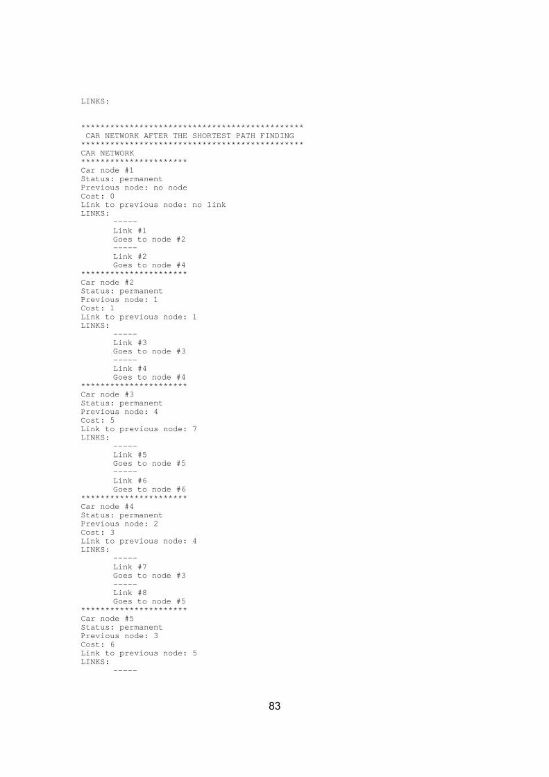
83

LINKS: ********************************************** CAR NETWORK AFTER THE SHORTEST PATH FINDING ********************************************** CAR NETWORK ********************** Car node #1 Status: permanent Previous node: no node Cost: 0 Link to previous node: no link LINKS: ----- Link #1 Goes to node #2 ----- Link #2 Goes to node #4 ********************** Car node #2 Status: permanent Previous node: 1 Cost: 1 Link to previous node: 1 LINKS: ----- Link #3 Goes to node #3 ----- Link #4 Goes to node #4 ********************** Car node #3 Status: permanent Previous node: 4 Cost: 5 Link to previous node: 7 LINKS: ----- Link #5 Goes to node #5 ----- Link #6 Goes to node #6 ********************** Car node #4 Status: permanent Previous node: 2 Cost: 3 Link to previous node: 4 LINKS: ----- Link #7 Goes to node #3 ----- Link #8 Goes to node #5 ********************** Car node #5 Status: permanent Previous node: 3 Cost: 6 Link to previous node: 5 LINKS: -----

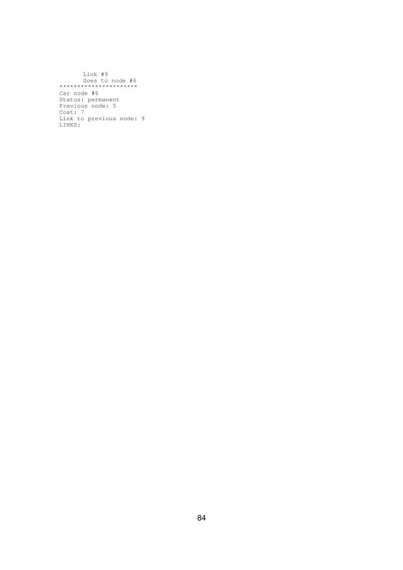
84

Link #9 Goes to node #6 ********************** Car node #6 Status: permanent Previous node: 5 Cost: 7 Link to previous node: 9 LINKS: