INTERNATIONAL BLACK SEA UNIVERSITY

FACULTY OF COMPUTER TECHNOLOGIES AND ENGINEERING

PhD PROGRAM

INCREASE OF PERFORMANCE AND EFFECTIVENESS OF THE MULTI DEPOT VEHICLE ROUTING PROBLEM’S SOLUTION (ON THE

EXAMPLE OF SOUTH CAUCASIAN LOGISTICS NETWORK)

Artioma Merabiani

Doctoral Dissertation in Computer Sciences

Tbilisi, 2017

Scientific Supervisor: IRAKLY RODONAIA

Professor, Doctor at International Black Sea University

I confirm that the work corresponds to the field, is characterized by novelty, scientific and practical value and is presented by the format defined by International Black Sea University.

________________________________________________ (supervisor’s signature)

Experts (full name & academic title):

1. Professor, Doctor Alexander Milnikov

2. Professor, Doctor Nodar Momtselidze

3.

Opponents (full name & academic title):

1. Professor, Doctor Guram Lezhava

2. Professor, Doctor Bibigul Koshoeva

3. Assoc. Professor, Doctor Khatuna Bardavelidze

I acknowledge that this is my own work, which is presented in the format defined by International Black Sea University and is attached by the publications relevant to the dissertation.

________________________________________________ (doctoral student’s signature

CONTENTS

LIST of FIGURES ............................................................................................................................ i

Abbreviations .................................................................................................................................. v

Introduction ..................................................................................................................................... v

Chapter I – Literature Review ......................................................................................................... 5

1.1 Problem review ..................................................................................................................... 5

1.2 Vehicle Routing Problem ................................................................................................ 12

1.2.1 Capacitated VRP (CPRV) ............................................................................................. 15

1.2.2 Multiple Depot VRP (MDVRP) .................................................................................... 15

1.2.3 Periodic VRP (PVRP) ................................................................................................... 16

1.2.4 Split Delivery VRP (SDVRP) ....................................................................................... 16

1.2.5 Stochastic VRP (SVRP) ................................................................................................ 16

1.2.6 VRP with Backhauls ..................................................................................................... 16

1.2.7 VRP with Time Windows (VRPTW) ........................................................................... 17

1.2.8 VRP with Satellite Facilities ......................................................................................... 17

1.3 Traveling Salesman Problem ............................................................................................... 17

1.3.1 The closest neighbor heuristics ..................................................................................... 24

1.3.2 Greedy heuristic ............................................................................................................ 25

1.3.3 Insertion heuristic .......................................................................................................... 26

1.3.4 Christofide heuristic ...................................................................................................... 26

1.3.5 Lin-Kernighan ............................................................................................................... 27

1.3.6 Tabu search ................................................................................................................... 28

1.3.7 Simulated annealing ...................................................................................................... 28

1.3.8 Ant colony optimization ................................................................................................ 28

1.4 Algorithms ........................................................................................................................... 30

ii

1.4.1 Genetic algorithms for VRP .......................................................................................... 30

1.4.2 Cross entropy in VRP .................................................................................................... 33

1.4.3 Branch and Bound algorithm ........................................................................................ 34

1.4.4 Evolution Algorithms .................................................................................................... 35

1.4.5 Adaptive large neighborhood search ............................................................................. 37

1.5 Tools .................................................................................................................................... 42

1.5.1 GraphHopper ................................................................................................................. 42

1.5.2 Openstreetmaps ............................................................................................................. 42

1.5.3 jRESP ............................................................................................................................ 43

1.5.4 MatSim .......................................................................................................................... 44

1.5.5 DEECo .......................................................................................................................... 48

1.6 Chapter I Summary .............................................................................................................. 52

Chapter II Methodology ................................................................................................................ 53

2.1 Planning initial routes .......................................................................................................... 53

2.1.1 Counting minimal number of vehicles .......................................................................... 57

2.2 Example review ................................................................................................................... 63

2.2.1 Parameters ..................................................................................................................... 63

2.2.2 Calculation .................................................................................................................... 63

2.2.3 Travel time and traveled kilometers .............................................................................. 64

2.3 Chapter II Summary ............................................................................................................. 66

Chapter III Adaptive real-world algorithm of solving MDVRPTW ............................................. 67

3.1 Adaptive real-world algorithm of solving MDVRPTW (Multi Depots Vehicle Routing

Planning with Time Windows) problem [25] ............................................................................ 67

3.2 Chapter III Summary .......................................................................................................... 78

Chapter IV Application Of DEECo ............................................................................................... 79

4.1 Application Of DEECo Framework To MDVRPTW Problem ........................................... 79

iii

4.2 Cloud computing [34] .......................................................................................................... 88

4.2.1 Private cloud .................................................................................................................. 90

4.2.2 Public cloud ................................................................................................................... 90

4.2.3 Hybrid Cloud ................................................................................................................. 90

4.2.4 Software as a Service .................................................................................................... 91

4.2.5 Platform as a service ..................................................................................................... 91

4.2.6 Infrastructure as a Service ............................................................................................. 91

4.2.7 CloudSim ....................................................................................................................... 92

4.3 Chapter IV Summary .........................................................................................................114

Conclusion and Future Works .....................................................................................................115

References and Literature ............................................................................................................118

iv

LIST of FIGURES FIGURE 1 PLATFORM PLAN .................................................................................................................. 11 FIGURE 2 FLOW CHART......................................................................................................................... 20 FIGURE 3 THE CLOSEST NEIGHBOR HEURISTICS ........................................................................... 25 FIGURE 4 GREEDY HEURISTIC ............................................................................................................ 25 FIGURE 5 INSERTION HEURISTIC ....................................................................................................... 26 FIGURE 6 CHRISTOFIDES HEURISTIC ................................................................................................ 26 FIGURE 7 LIN-KERNIGHAN ................................................................................................................... 27 FIGURE 8 PSEUDO CODE FOR EVOLUTIONARY ALGORITHM APPROACH ............................... 36 FIGURE 9 PSEUDO CODE FOR CO-EVOLUTIONARY ALGORITHM .............................................. 37 FIGURE 10 LARGE NEIGHBORHOOD SEARCH ................................................................................. 38 FIGURE 11 ADAPTIVE LARGE NEIGHBORHOOD SEARCH ............................................................ 39 FIGURE 12 SCEL ....................................................................................................................................... 44 FIGURE 13 PSEUDO- CODE FOR MATSIM COEV. PRINCIPLE ........................................................ 46 FIGURE 14 MATSIM OUTPUT OF TRAFFIC AT 07:30 IN THE MIV (10% SAMPLE) EXAMPLE OF

SIMULATION IN CITY VORARLBERG [38] DOTS REPRESENT VEHICLES. ......................... 47 FIGURE 15 MATSIM TOOLKIT [46] ...................................................................................................... 48 FIGURE 16 DEECO SCHEME .................................................................................................................. 51 FIGURE 17 NUMBER OF VEHICLES ..................................................................................................... 58 FIGURE 18 SERVICE PARAMETERS .................................................................................................... 59 FIGURE 19 CARGO LOAD ...................................................................................................................... 60 FIGURE 20 OPTIMAL ROUTES GENERAL VIEW ............................................................................... 61 FIGURE 21OPTIMAL ROUTES CLOSER LOOK AT TBILISI CUSTOMERS ..................................... 61 FIGURE 22 COORDINATES .................................................................................................................... 62 FIGURE 23 OPTIMAL SOLUTION .......................................................................................................... 65 FIGURE 24 FUNCTIONAL DESCRIPTION OF A COMPONENT ........................................................ 68 FIGURE 25 GENERAL INFRASTRUCTURE.......................................................................................... 70 FIGURE 26 EXPECTED CONGESTION-INDUCES DELAY ................................................................ 74 FIGURE 27 ROUTESEGMENTAVAILABILITYAGGREGATOR ........................................................ 83 FIGURE 28 JDEECO RUNTIME FRAMEWORK ARCHITECTURE. ................................................... 87 FIGURE 29 CLASS DESIGN DIAGRAM FOR CLOUDSIM .................................................................. 94 FIGURE 31COMPONENTS OF THE SOFTWARE SYSTEM FOR MODELING PRIVATE CLOUD

PAAS-SYSTEMS ............................................................................................................................. 110 FIGURE 32 COMPONENTS CLOUDSIM[45] ....................................................................................... 112

v

Abbreviations

• AC – Autonomic Component • ACE– Autonomic Component Ensembles • ALNS - Adaptive Large Neighborhood Search • API - Application Programming Interface • B&B - Branch and Bound

• BPP - The Bin Packing Problem • COP - Combinatorial Optimization Problems

• CPRV - Capacitated VRP

• DEECo - Dependable Emergent Ensembles of Components • EBCS - Ensemble- Based Component Systems • jRESP - Java Run-time Environment for SCEL Programs • LNS - Large Neighborhood Search

• MAP - Modified Assignment Problem

• MDVRP - Multiple Depot VRP

• mTSP - multi Travelling Salesman Problem

• POIs - points of interest • PVRP - Periodic VRP

• QA - Quasi-Assignment

• SCEL - Software Component Ensemble Language • SDVRP - Split Delivery VRP

• SECs - Subtour Elimination Constraints

• SRD - database of simulation results • sTSP - symmetric Travelling Salesman Problem

• SVRP Stochastic VRP

• TCMD - travel and congestion management database • The MATSim - Multi-Agent Transport Simulation)

• TRANSIMS - TRansportation Analysis and SIMulation System • TSP - The Traveling Salesman Problem • VRP - Vehicle Routing problem • VRPTW - VRP with Time Windows

• VRPTW -The Vehicle Routing problem with Time Windows

1

Introduction

The thesis examines the value of real-time traffic information for optimal vehicle routing in a non-

stationary stochastic network. Our goal is to develop a systematic approach to aid in the

implementation of transportation systems integrated with real-time information technology. Based

on many researches done in the fields of VRP and TSP we can implement them for our heuristics.

Finding ways to develop decision making procedures for determining optimal driver attendance

times optimal departure times, and optimal routing policies under stochastic time-changing traffic

is firsthand goal of our research. With studies based on a road network in Georgia, we demonstrate

significant advantages when using this information in terms of total costs savings and vehicle

usage reduction while satisfying or improving service levels for just-in-time delivery. With such

systems routing and controlling traffic and vehicles should be done more in more precise and easy

manner. That means that many sectors of logistics industry can improve their work and make their

services cheaper, that will also influence end-user. Our algorithm is adaptive and can react to

number of stochastic effects and constrains that can be observed in real logistics networks.

Goals of Research:

Main goal of the following research is to investigate existing approaches in the area of multi depot

vehicle routing problem, to reveal its suitability to the practical needs of the Georgian logistic

network and to develop new techniques and methods which will satisfy above mentioned needs.

In particular, the following issues have to be developed in the thesis:

• A theoretical approach that can manage the uncertainty and stochastic nature of VRP in

real life environment.

• Mathematical models which can accurately predict transportation stochastic parameters

such as traffic volumes, congestion induced delays etc.

• Combination of models, algorithms and applied technical tools which will ensure the

search of practically acceptable optimal routes and usage of advanced technologies. Also

the framework to be developed must provide users ability to modify routes in simultaneous

and parallel manner.

2

• Modification of widely used ALNS algorithm (which cannot be directly used for practical

needs of logistics networks being under investigation); this modification must be directly

applicable to the conditions of Georgian transportation network.

• A suitable programming framework which can effectively implement developed heuristics

and algorithms must be accurately selected or developed from scratch.

• Detailed research of all statistical data, which may have important impact on the main

traffic characteristics (like types of road congestions, delays, etc.,) on areas of interest. In

case of absence of such data, reliable methods of determination and obtaining such

information must be developed in the thesis.

• Convenient programming tools which help developed methods to be effectively

implemented in practice must be selected.

• Technical implementation of proposed approaches and algorithms must be maximally cost

effective.

Importance (significance)

Logistic networks and their tasks are nowadays most important area, from the stand point of vitally

importance of Georgian logistic network in the context of increasing demand of international

shipments (Silk road). Existing logistics network is not yet developed to satisfy these increasing

requirements. Moreover, known to us algorithmic methods and techniques do not cover practical

and realistic needs of (Silk road) international shipments. Therefore, there is an urgent need to

develop relevant approaches and methods which can fully satisfy above mentioned problems and

tasks. Those approaches and methods have to increase throughput of logistic network and generate

significant economic effect. Modern society needs a constant increase in the volume of transport,

increasing its reliability, safety and quality. This requires increasing the cost of improving the

infrastructure of the transport network, turning it into a flexible, highly regulated logistics system.

At the same time, the risk of investment increases significantly if the patterns of the transport

network development are not taken into account, providing that the distribution of the loading of

its sections is taken into account. Ignoring these patterns leads to the frequent formation of traffic

jams, overload / underload of certain lines and nodes of the network, increasing the level of

accidents, environmental damage. The theory of transport flows was developed by researchers of

various fields of knowledge - physicists, mathematicians, operations research specialists, transport

workers, economists. A wide experience of studying the processes of motion has been

accumulated. However, the general level of research and its practical use is not sufficient.

3

Theoretical Value

As it is known, large variety of theoretical methods exists in this area. However, they can’t satisfy

practical requirement of Georgian logistics network, in particular with increasing impact of new

developed intentional Silk Road logistic network. Most of existing nowadays heuristics cannot

provide full specter of solutions for real life logistics networks. This theoretical framework will be

used as a base for the practical and concrete algorithms. For example, in the existing paradigm,

uncertainty and stochastic nature of the VRP is not fully reflected. With this in mind new

theoretical approaches (accounting for practical needs of real environment) have been developed

in the thesis. The solution of such problems is impossible without mathematical modeling of

transport networks. The main task of mathematical models is the definition and forecast of all

parameters of the transport network functioning, such as traffic intensity on all network elements,

traffic volumes in the public transport network, average traffic speeds, delays and time losses. All

the said above was implemented in the approach of the thesis and has great importance for the

future researches

Practical Value

As it was pointed out above, practical needs of Georgian logistics network require new approaches

to satisfy realistic problems and tasks. Therefore, techniques developed in the thesis will have

undoubted practical values and they will be able to bring significant economic effects and

contributions. As already pointed above these economic gains will affect end-users in many fields.

Transport infrastructure is one of the most important infrastructures in the life of cities and regions.

In recent decades, many large Cities are exhausted or close to the exhaustion by the extensive

development of transport networks. Therefore, optimal planning of networks, improvement of

traffic organization, optimization of the system of public transport routes has a practical

importance. All mentioned above results in increasing practical value of the thesis.

Novelty

In the thesis a new set of algorithms and applied tools which combine the application of known

algorithms for searching optimal routes (taking into account the actual conditions on the sections

of planned routes) and usage of new technology of autonomous components ensembles, has been

developed. In particular, the developed program complex allows users to modify promptly

current routes based on local information and choose the most accessible routes which reflect

local real situation. The originality of the developed complex also lies in the fact that all the

4

necessary calculations are made by the autonomous components, associated with specific cars, in

virtual machines of datacenters. This allows users to modify routes in simultaneous and parallel

manner without the need to install expensive equipment and software in vehicles. The later

significantly reduces the duration and cost of the necessary calculations. The technology

developed in the thesis will also help to improve the efficiency and safety of traffic planning for

unmanned vehicles.

Research Methods

In the thesis the following methods have been used:

• Collection and classification and estimation of necessary data.

• Modeling and simulation for obtaining required important parameters and characteristics

of processes involved in the research.

• Intensive usage of global optimization methods.

• Developing and usage of wide specter of programming solutions.

• Deployment of modern advanced technical solutions to provide maximum effectiveness

of proposed models and algorithms, which may result in significant reduction of costs.

Thesis Limitations Due to the non-availability of data for Armenia and Azerbaijan logistic networks this dissertation

is based on realistic information for Georgian logistics network. However, all of the developed

methods and algorithms can be applicable to Armenian and Azerbaijan logistics network without

significant changes.

5

Chapter I – Literature Review

1.1 Problem review

Transport logistics is becoming an increasingly important component of many areas of activity. In

commerce, the share of transportation costs for a product may be 25-35% of its value. In 2010-

2014. The volume of the market for commercial road freight transport has more than doubled. This

situation imposes high demands both on representatives of freight services and on producers of

goods. Transportation also uses most part of petroleum (Fuglestvedt et al.,2008). Optimization of

transportation becomes a serious competitive advantage.

In the past, the compilers of vehicle routes and controllers acted independently of each other and

without information exchange, or only with very little. The location of vehicles on the route line

was not known, and it was not always possible to establish a good connection with the driver.

Recent advances in information and communication technologies have significantly improved the

quality of communication between the driver and the dispatch center. Now, information on the

arrival of new orders or changes in routes can easily be passed on to drivers, which helps to

improve the level of service and reduce costs.

A direct supply chain consists of a producer of a finished product (a focus company), a supplier

(level 1), a consumer (level 1), who directly participate in the external and internal flow of

products, finance and information. Most often, the focus company determines the structure of the

supply chain and management of relationships with business counterparties. The order of

interaction of participants in it is determined by the conditions of the external environment

(random and deterministic indicators that affect the level of production, the structure of purchases

of raw materials, the policy of distribution of finished products to end users, including the

transportation policy).

The expanded supply chain includes additional suppliers and second-tier consumers. The extended

supply chain is the basis for constructing a reference model of operations in supply chains, since

such a basic chain structure is most common in business.

6

The maximum supply chain consists of a focus company and all its counterparties (down to source

suppliers) that determine the resources of the focus company at the entrance, and the distribution

networks on the right - down to the end users.

Complex, branched relationships between suppliers and consumers in various industries imply the

identification and study of the behavior of the relevant participants in various supply chains. In the

modeling of supply chains, the multi-product mix of products, temporary, territorial and cost

constraints, the random nature of some logistics processes in supply chains are taken into account.

The need for constant movement of raw materials, semi-finished products, finished products,

materials and containers by means of transport between participants in the supply chains of the

industry makes for increased requirements for a key logistic function - transportation. The lack of

a methodology for transport management at industrial enterprises at the marketing stage leads to a

disruption in the schedule of deliveries, uneven exports of finished products, incomplete use of the

carrying capacity of vehicles, and therefore increases the costs of rolling stock operation and the

price of products. At the procurement stage, untimely delivery leads to an increase in the average

level of stocks of raw materials and materials, the creation of increased insurance reserves, the

disruption of the production schedule and rhythm and, as a result, an increase in the cost of finished

products. The variety of transport links between suppliers and consumers, the use of the rolling

stock of transport enterprises of various forms of ownership, necessitates the application of a

systematic approach to the choice of ways of interaction between industrial enterprises and

suppliers of raw materials, trade and transport organizations. Since the goal of any enterprise in

the industry is to increase profit, and in the financial sphere - to shorten the duration of the

operational and financial cycles, the choice of rational ways of managing transportation can

positively affect the financial performance of enterprises. The tasks of transport and logistics

services are being addressed at the strategic, tactical and operational levels. The objectives of the

strategic level allow you to design a network for promoting the material flow, determine the

location of the main and auxiliary objects of service, identify schemes for the movement of

industrial goods between them, determine the tariff policy, and develop strategic transportation

plans. At the tactical level, the plans, routes of transportation, the order of service are adjusted,

taking into account the unevenness of demand, the availability of rolling stock at the nodes of the

supply chains, and so on. At the operational level, the tasks of assigning drivers' crews, the

development of routes and schedules of supplies for the next day are being decided. In the event

of a change in the results of solving the tasks of the operational level, corrections are also made in

the plans for the tactical and strategic levels. To fully satisfy the needs of supply chains in

7

transportation, several types of routing tasks have been identified, which depend on the restrictions

and requirements imposed on the delivery system. The application of the appropriate type of task

and combination of tasks in the logistics industry depends on such factors as the time range of

customer service (the "time window"), the centralization and decentralization of delivery (several

senders), the ability to organize the collection and delivery of products for a single transport cycle,

For several flights to each consumer, etc. In view of the fact that the dimension of the routing task

in logistics is quite large due to the complex marketing network, in practice, heuristic and meta-

heuristic methods are often used to obtain a qualitative solution, the use of which allows obtaining

acceptable results in a relatively short time. When choosing the type of task, factors such as the

planning horizon, the method of controlling the level of stocks, the type of demand for products,

the number of types of deliverables in supply chains, the number and carrying capacity of vehicles,

routing policies, inventory accounting and management are taken into account. Solving the

problems of joint inventory management and routing allows you to obtain results that contribute

to making decisions about choosing or changing the strategy of inventory management, building

or modernizing transport policy, harmonizing transport and storage processes, integrating them

with production processes in order to improve the efficiency of logistics industry enterprises

Supply chains.

This dissertation discusses the problem of routing vehicles with time windows and in real-time

conditions. To improve the efficiency of operational management, it is expected to use information

and communication systems based on mobile technologies. This includes, first of all, mobile

communication in real time between the control center and the drivers. Thus, new instructions can

be communicated to drivers, even if they have already left the point of departure and are on the

way to the client. Secondly, the datacenter can determine the geographic location of the vehicle on

the road with the help of modern navigation systems (GPS). At all times, knowledge of the spatial

orientation of physical objects or, to put it simply, of their geographical location, were very

important for people. For example, primitive hunters always knew the location of their prey, and

the life or death of explorers of the pioneers directly depended on their knowledge of geography.

Also, modern society lives, works and cooperates, relying on information about who and where is

located. Applied geography in the form of maps and information about space helped to make

discoveries, promoted trade, increased the safety of human life for at least the last 3000 years, and

maps are one of the most beautiful documents that tell about the history of our civilization

This contributes to the efficient operation of the fleet and increases productivity. And, thirdly,

modern technology can provide information about the current traffic situation on the road. This

8

makes it possible to consider the timing of transport with a temporary dependency, constantly

updated during the day. All the aforementioned possibilities of using mobile technologies allow

reacting to certain dynamic events, such as interference on the roads and changing the route of the

vehicle in real time.

Routing of shipments to the sender and stepped routes is carried out by scheduling the loading in

different directions on certain days. Scheduling allows you to organize routes from cargo trucks

by several consignors, when the size of loading for each of them for the route is insignificant. As

already mentioned above, for the transport of bulk goods between regular senders and recipients

in specific conditions apply special sender routes, which are called ring routes. Such routes are

addressed between the stations of their loading and unloading according to strictly established

timetables, and from the loading stations they are always sent with the same cargo, and they are

returned empty or with a different cargo.

Road transport carries a large number of bulk cargo: construction (land, sand, gravel, crushed

stone, brick, panels, farms, timber), agricultural (grain, cotton, sugar, Beetroot, vegetables), fuel

(coal, firewood, peat), trade, etc. The production and transportation of bulk goods causes a very

intensive turnover associated with the placement of cargo-carrying and cargo-absorbing posts and

the establishment of transport links between them.

The location of loading and unloading points in the transport of bulk goods, as a rule, creates a

constant, characteristic for the structure and capacity of cargo flows, changing mainly in a planned

order. The mass and intensity of cargo flows between the permanent points of departure and arrival

create exceptionally favorable conditions for the organization of route traffic carried out by a

special group (column) of cars.

Route shipments are made according to the schedule, developed on the basis of the data of the

monthly and operational shift-daily plans. With good and precise organization of loading and

unloading operations, scheduled transportation is carried out according to the schedule and the

schedule of rolling stock movement.

Especially in case of scheduled mass transportations, the use of road trains and special trains to

increase the productivity of transportation. If there are enough trailers, loading and unloading

facilities, as well as favorable road conditions, the use of road trains is effective for the transport

of bulk goods: it allows better use of the traction power of the car and increase the carrying capacity

9

(the total carrying capacity) of the rolling stock. This organization of transportation reduces the

cost of transportation by more than 20%.

For this research we assume that we have logistic (distribution) company with fleet of standard

cargo vehicles and there are our multiple depots located in different cities and districts of Georgia.

The search for optimal transport routes is a key task in the field of logistics. Each depot has

individual working hours’ schedule. There are many different customers in different cities, each

customer has specific demand in goods and specific time window when they need to be served and

also other constrains such as start of the working day hours and time that is needed to unload the

cargo (service time). Many different constrains should be considered for example, vehicle cargo

payload, distance traveled with one tank of gas and so on. Also we consider that problem of

congestions is requiring most of the attention. We have to use such algorithm that will make

decisions whether to avoid traffics jams or congestions or to wait until road is free, so that this

particular vehicle wont violate its scheduled plan and specific time window constrains of the

customer. This information about traffic jam and congestions also should be shared to other

concerned vehicles so that if their route also lies through congested area their AC should re-plan

schedule or routing again not to violate any time windows.

Because of lack of information and statistics about traffic in Georgia and Tbilisi, we have to use

different approach. We can’t make predictions for routing without knowing real life situation on

road and statistical data from database for every street or road in Georgia. It means that firstly

planner should be filled with some data, in our case we assume that with the help of MATSim we

can run multiple simulations and make statistics for our knowledge bases. MATSim can show

bottleneck zones on Georgia map, so we can assume that this areas with high car traffic can be

considered as highly congestion danger areas. After receiving basic statistical data algorithm can

obtain new information daily from every individual depot and every individual vehicle with help

of AC assigned to each. This framework based on ACEs will generate new data and will correct

statistical data received from MATSim simulations. It will grant high quality information for

planning algorithms to schedule every day plan for whole fleet of vehicles.

Our goal is to maximally automate scheduling and planning routes and further control of vehicles

and granting drivers with up-to-date information about possible difficulties in their route.

Algorithms and framework have to work stable and fast, while taking in account stochastic nature

of traffic flow and possible unplanned delays. Maximal automation means that each vehicle should

be equipped with GPS and every driver has to have Smartphone to receive information about

10

routes, plans and possible difficulties ahead on the road and routes to avoid them. So that

datacenter can control process flow. As mentioned above each vehicle should be equipped with

nowadays gadget and ACE has to have each AC assigned to each individual vehicle and depot.

Also such kind of algorithm has to be flexible enough for concerning backhauls vehicle accident

and many other unpredicted factors. It is obvious that such a huge framework won’t be able to

always complete every task that is given due to a stochastic nature of traffic itself. So we consider

that it should get closest to optimal solution, to minimize total expenditure of the company and

serving highest possible number of customers daily. If still many casualties occur daily algorithm

has too find solution for solving this issue for example advising to add vehicles to fleet or maybe

to add new depots in different locations.

For that kind of problem specific platform has to be created. Which will include different

algorithms and systems. As shown in fig1.

1. This platform has to receive orders from customers.

2. Count minimal possible number of vehicles, to minimize cost of transportation.

3. Plan optimal routes for drivers with minimal travel cost and not violating capacity and time

window demands

4. Share the information and give exact route on map to drivers.

5. Based on agent based modeling, agents should distribute duties for each driver.

6. Notify drivers about traffic and possible difficulties on their route. And in case of

congestion should give another available route to avoid traffic.

11

Figure 1 Platform plan

12

1.2 Vehicle Routing Problem

In the theory of computational complexity, it is customary to consider recognition problems

(properties), that is, problems in which the possible answer is "Yes" or "No". For example, is it

true that a given graph is a tree? Among the recognition tasks, it is customary to select the classes

P and NP. We recall that the class P consists of recognition problems that are solvable in

polynomial time. The NP class is broader. It includes all recognition tasks in which the answer

"Yes" can be checked for polynomial time. The task belongs to this class, if, even without knowing

how to solve it, it is possible to "easily" check the answer, having peeked it or found it on the

Internet. Thus it is enough to be able to check only the answer "Yes". Sometimes checking the

answer "Yes" may be easier or more difficult than checking the answer "No". We consider the

problem of the Hamiltonian property of a graph: given a simple undirected graph, it is required to

know whether it contains a Hamiltonian cycle? We show that this problem belongs to the class

NP. Suppose that the graph is indeed a Hamiltonian, and someone has given us an answer,

indicating one of these cycles. (Harnoor K. 2013)

Modern transport, and in particular the street infrastructure, is increasingly encountering

bandwidth limits. The existing system of organizing transportation in conditions of increasing

density of the route network does not always satisfy the emerging demand for transport services.

As infrastructure expansion activities can hardly meet the uncontrollable growth in the number of

transport units on city streets, the planning tasks for transportation are beginning to change. The

complexity of the task requires new forms of planning, or at least changes in the emphasis of traffic

planning. The task of transport routing can be solved by building one or several ring routes. For

their construction, both methods of exact linear programming and approximate heuristic methods

are known. It is necessary to take into account that before using these or other methods, they must

be tested for applicability depending on certain parameters of the traffic routes.

Can I check this tip for polynomial time? To do this, we need to verify that the specified set of

edges forms a simple cycle, and it covers all vertices. Obviously, this is "easy" to do and,

consequently, the problem belongs to the NP class. Note that the answer "No" is much harder to

check here. It is said that the recognition problem belongs to the class co-NP, if the answer "No"

can be checked for polynomial time. It is easy to show that the next problem belongs to the class

ω-NP. Given a simple undirected graph, is it true that it is not Hamiltonian? Answer "No" means

that the graph is Hamiltonian, and this can be easily verified. In the class P one can check with any

polynomial complexity, and therefore P ⊆ NP. To prove or refute the reverse inclusion so far no

13

one manages. To date, this is the bottom of the central problems of mathematics - the "Millennium

Challenge"

Vehicle Routing problem (VRP) has been delineated along with outlined, quite thirty years past.

VRP is the hardest optimization combinatorial problem. (Eberhardt et al., 1991) (Dyckhoff et al.,

1997) VRP is represented as “For every specific list of POIs (points of interest) with specific

range of vehicles, cargo should be delivered to every customer”. Main challenge is to make

minimum (the optimum) list of (routes) for specific range of vehicles. The difficulty in applying

this problem to the real life circumstances, is in stochastic behavior of traffic and plenty of

additional constrains.

For this extremely complicated combinatorial optimization problem, both exact and approximate

algorithms have been proposed.

Interest in such problems is due not only to their great applied value, but also to the complexity of

the solution. A number of reviews and monographs on this topic have been published. Of the most

significant are the works of P. D. Christofides, G. Laporte, M. Solomon.

Using nowadays technologies and completely different approaches, lots of latest studies were

created during this field. Individual still manage to imply novelties in on 1st sight recent problems

like VRP. The vehicle routing problem refers to any or all issues where best closed-loop system

methods that touch completely different points of interest, like during this case cities and countries.

VRP may be a general name that was given to the issues and tasks wherever a listing of finish

points or POIs for variety of vehicles positioned at one or multiple depots should be determined

for variety of geographically placed customers or cities. There may be one or plenty of cars within

the fleet, additionally one or multiple depots, POI and different further factors. Goal is minimizing

price of the transportation. whereas satisfying all the customers with their demands minimum

vehicles ought to be concerned so as to avoid wasting fuel and cash, however at same time all the

constrains ought to be taken into consideration and not desecrated.

This particular challenging combinatorial problem was created from the concepts of two well-

known problems such as problem (TSP) and (BPP)

The Traveling Salesman Problem (TSP): In fact, TSP can be transformed in VRP by changing

some parameters. There is even multiple Traveling salesman problem which is generalization of

original TSP, but with more then, one Salesman.

14

The Bin Packing Problem (BPP) (Dyckhoff, et al., 1997).: Is described as follows: “Given the set

of items and their weights, we have to place all items in minimal number of bins” BPP is also NP-

hard problem.

In the fields of transportation, supply chain and logistics main problem to define is The Vehicle

Routing problem. Largely in all told market fields, transportation logistics and supply chain adds

a major share to the value of the products. Therefore, automation processes for supplying field

usually lead to high value economy starting from five percent to twenty of the whole worth. In real

world things in VRPs, lots of further constraints appear.

Real world applications of the VRP, in contrast with its accepted definition, often includes two

important aspects: evolution of information and quality of information. Quality of information

reflects possible uncertainty on the available data, for example when the demand of a client is only

known as an estimation of its real demand, that means that in many case planner should behave

according to unreliable data. Evolution of information means that while planning initial plan,

planner has to consider that during execution of the process, many things can happen.

Generally, the points of interest are mentioned as nodes. In our study, the beginning and finish

points of a route are identical and are referred to as the depots. several sub issues occur in common

Vehicle Routing problem one in all them that we tend to use during this paper is extension of VRP

- The Vehicle Routing problem with Time Windows (VRPTW) it's known as non-polynomial hard

(NP hard) problem (Lenstra et al., 1981). This VRP involves range of vehicles (fleet) that has to

serve given totally different customers with specific demands and distinctive time windows for

every. Customers are settled in numerous geographic locations. additionally each vehicle should

come at finish point (depot) by the end of the operating day. Objective of the VRPWT is finding

greatest optimal solutions to navigate the fleet so as to serve every clients with minimal value

(counting gas and salaries in terms of traveled distances) while not violating capacity and time

period constraints of every vehicle and distinctive customer demanded time windows.

There are a lot of different cases of VRPs in our paper only few will be used, but to have general

knowledge of VRP, there are some most used described with their main goals (objectives):

15

1.2.1 Capacitated VRP (CPRV)

CVRP may be a Vehicle Routing problem wherever there's outlined range of vehicles with

constant capacity should deliver consignment to outlined customer demands for one sort of cargo

from a set depot with minimal transportation prices. CPRV considers that there's just one sort of

cargo. Main goal is minimizing transportation value for delivering company. And also reducing

quantity of vehicles used and considering amount of cargo not to violate capacity constraints.

Solution will be feasible if all the above is included.

The CVRP is outlined more exactly as follows. we are given an directionless graph 𝐺𝐺 =

(𝑉𝑉, 𝐸𝐸)with vertices 𝑉𝑉 = 0, . . . , 𝑛𝑛 wherever vertex zero is that the depot and therefore the

vertices 𝑁𝑁 = 1, . . . , 𝑛𝑛 are customers. every edge e ∈ E has an associated value 𝐶𝐶𝑒𝑒. The demand

of every customer i ∈ N is given by a positive amount 𝑞𝑞𝑖𝑖.. Moreover, 𝑚𝑚 uniform vehicles are

accessible at the depot and also the capability of every vehicle is up to 𝑄𝑄. The goal of the CVRP

is to seek out precisely 𝑚𝑚 routes, beginning and ending at the depot, such every client is visited

precisely once by a vehicle and such the total of demands of the customers on every route is a

smaller amount than or up to 𝑄𝑄. The total of the edge worth employed in the m routes should be

reduced. (Golden et al., 1998), (Altinel and Oncan 2005) (Toth and Tramontani 2008)

1.2.2 Multiple Depot VRP (MDVRP)

In Multiple Depot VRP (MDVRP) there is company with fixed number of vehicles and has

multiple depots. There are different approaches to solve this problem. First one is to assign some

concrete customers to each depot, and to solve VRP individually for each depot with its customers.

It is feasible if geographically assigned customer demand can be served exclusively with only one

depot. But there is also case when planner can distribute customers demand with different depots

if they are located reasonably close to each other geographically. In this case algorithms should

distribute equally demands and objective to minimize total cost of transportation.

(Hadjiconstantinou et al., 1998)

16

1.2.3 Periodic VRP (PVRP)

Main difference between standard VRP and Periodic VRP is that, in classic VRP schedule and all

calculations are made for only one working day while in PVRP palling is done for undefined

number of days. A solution is feasible if all constraints of VRP are satisfied. However, a specific

vehicle or number of vehicles may not return to the depot in the same day from its departure. Over

some undefined period, of course taking into account that individual customer must be visited at

least once. (Christofides et al., 1984) (Potvin and Rousseau 1993) (Vidal et al., 2012)

1.2.4 Split Delivery VRP (SDVRP)

SDVRP is type of VPR where each customer is served by different vehicles. Main difference from

classic VRP is allowance of vehicles to visit each other’s POIs, if total cost is reduced and if

customers demand is as equal or more then the capacity of company’s standard vehicle. A solution

is feasible if all constraints of VRP are satisfied excepting allowance of multiple different vehicles

to deliver goods to individual customer. (Dror et al., 1994)

1.2.5 Stochastic VRP (SVRP)

Stochastic VRP is one of the most realistic and close to real-life situation (Bertsimas et al., 1997).

Stochastics VRP means that one or more variables are completely random. It means that for every

day scheduling planner should consider that customers, demand and service times are completely

random and stochastic. In fact, it splits problem on two. Firstly, planner should determine all

variables and then after getting information it should make standard calculations of VRP.

1.2.6 VRP with Backhauls

The Vehicle Routing Problem with Backhauls (VRPB) is a type of VRP where each individual

customer can demand return goods to a depot. Main constrain here is that vehicle capacity should

be considered and fact of that the vehicles have rear load also rearranging of goods also leads to

additional costs. Solution is feasible if set of routes is found that satisfy the demand and backhauls.

While saving total cost.

17

1.2.7 VRP with Time Windows (VRPTW)

The VRPTW is VRP where additional constrain is added such as time windows. In our paper we

consider this constrain along with others. Main problem is to set routes and timing not to violate

lower or upper bounds of time windows, while minimizing cost of transportation including waiting

time of vehicles because each customer has specific individual time windows. The solution is

feasible if all of the constrains are considered. Heuristics for solving was proposed by (Braysy et

al., 2005) If customer is served with violation of lower or upper bounds solution becomes

unfeasible. Also planning should be done that way, that vehicles minimize waiting time because

additional waiting time adds additional cost to total transportation cost.

1.2.8 VRP with Satellite Facilities

An important side of the vehicle routing problem (VRP) that has been for the most part unnoted is

that the use of satellite facilities to fill up vehicles throughout a route. once attainable, satellite

replenishment permits the drivers to continue making deliveries till the end of their shift while not

having to returning to the central depot. this example arises primarily within the distribution of

fuels and bound retail items. once demand is random, optimizing client routes a priori could lead

to important extra costs for a selected realization of demand. Satellite facilities are a method of

safeguarding against sudden demand.

1.3 Traveling Salesman Problem

VRP itself is based on The traveling salesman problem (TSP) which is one of the most intensively

studied problems in computational mathematics. TSP main problem to be solved as follows : “Given

a list of cities and the distances between each pair of cities, what is the shortest possible route that

visits each city exactly once and returns to the origin city? “

The traveling salesman problem (TSP) is one among the simplest to understand however anyway

NP-hard routing problem. The TSP aims to decrease total distances traveled by salesman.

The traveling salesman problem occupies a special place in combinatorial optimization and

operations research. Historically, it was one of those tasks that served as an impetus for the

development of these areas. The simplicity of the formulation, the finiteness of the set of

admissible solutions, the clarity and at the same time the colossal costs of a complete search are

still pushing mathematicians to develop new and new numerical methods. In fact, all fresh ideas

18

are first tested on this task. From the point of view of applications, it is not of interest. Much more

important is its generalization for the tasks of transporting goods and logistics, when several

vehicles of limited carrying capacity should serve customers by visiting them at specified time

windows.

In the classical task of the traveling salesman, all the details of real applications are absent. Only

the combinatorial essence is left, a purely mathematical problem that has not been managed for

half a century. It is this well-known problem that is devoted to this chapter.2. It includes all the

possible routes which cover every city possible on the route.

The TSP is divided in two types as symmetric travelling salesman problem (sTSP), (Gendreau et

al., 2005)

and multi travelling salesman problem (mTSP). This section presents description concerning these

2 wide studied TSP.

sTSP: V = 𝑉𝑉1,......, 𝑉𝑉𝑛𝑛 is a list of cities, A = (r,s) :r,s ∈V is list of nodes, and

𝑑𝑑𝑟𝑟𝑟𝑟= 𝑑𝑑𝑟𝑟𝑟𝑟 is a price attached to a node (r, s)∈ A.

Goal of the sTSP is to look up for the shortest closed tour while visiting each city once. In

this case cities 𝑣𝑣𝑖𝑖∈ V are shown by their geographic coordinates (𝑥𝑥𝑖𝑖 , 𝑦𝑦𝑖𝑖) and 𝑑𝑑𝑟𝑟𝑟𝑟is an Euclidean

interval from r to s in this case it is an Euclidean TSP.

aTSP: If 𝑑𝑑𝑟𝑟𝑟𝑟≠ 𝑑𝑑𝑟𝑟𝑟𝑟be for at least one (r, s) after this the ordinary TSP becomes an asymmetric one.

mTSP: The mTSP is outlined as: during a set of cities, we assume that there are 𝑚𝑚 salesmen

settled at a single depot node. The left cities that are not yet visited are in-between cities. After the

changes, the mTSP is about looking up for tours for every 𝑚𝑚 salesmen, that all start and end their

journeys at the same depot, specified every in-between city is visited exactly once and therefore

the end cost of visiting all nodes is decreased. the price metric may be outlined in terms of distance,

time, etc.

Possible variations of the problem comes, as follows: Single vs. multiple depots: within the single

depot, all salesmen end their tours at one point whereas in multiple depots the salesmen

can either come back to their initial depot or will come back to any depot keeping the initial range

of salesmen at every depot remains identical after the travel.

Number of salesmen: the quantity of salesmen within the problem are often fixed or a delimited

variable. Cost: once the quantity of salesmen isn't fixed, then every salesperson typically has an

19

associated fixed costs acquisition whenever this salesperson is employed. during this case, the

minimizing the wants of salesperson conjointly becomes an objective.

Timeframe: Here, some nodes ought to be visited in a very specific time periods, that is known as

time windows, that is an extension of the mTSP, and referred as multiple traveling salesman

problem with specified Timewindow (mTSPTW).

The application of mTSPTW are often fine seen within the aircraft planning issues. Other

constraints: Constraints are often on the quantity of nodes every salesperson will visits, maximum

or minimum distance a salesperson travels or the other constraints. The mTSP is usually treated as

a relaxed vehicle routing issues (VRP) wherever there's no restrictions on capacity. Hence, the

formulations and resolution ways for the VRP are equally valid and true for the mTSP if an

outsized capacity is assigned to the salesmen (or vehicles). However, once there's one salesperson,

then the mTSP reduces to the TSP.).

Connections with the VRP: mTSP can be utilized in solving several types of VRPs. discuss several

algorithms for VRP, and present a heuristic method which searches over a solution space formed

by the mTSP.

In a similar context, the mTSP are often used to calculate the minimum range of vehicles needed

to serve a group of consumers in a very distance-constrained VRP. The mTSP additionally seems

to be a primary stage drawback during a two-stage answer procedure of a VRP with probabilistic

service times. Scientists mentioned that the VRP instances arising in apply ar terribly laborious to

resolve, since the mTSP is additionally too complicated. This raises the requirement to

expeditiously solve the mTSP so as to attack large-scale VRPs.

The mTSP is additionally associated with the pickup and delivery problem (PDP). The PDP

consists of deciding the optimum routes for a group of vehicles to meet the client requests If the

purchasers are to be served at intervals specific time intervals, then the matter becomes the PDP

with time windows (PDPTW). The PDPTW reduces to the mTSPTW if the origin and destination

points of every request coincide.

Exact algorithms for the sTSP once (Dantzig et al., 1954) formulation was initially introduced, the

simplex technique was in its infancy and no algorithms were out there to resolve number linear

20

programs. The practitioners thus used a technique consisting of at first reposeful constraints and

therefore the integrality needs, that were bit by bit reintroduced when visually examining the

answer to the relaxed problem. (Martin, 1966) used an analogous approach. at first he didn't impose

higher bounds on the 𝑋𝑋𝑖𝑖𝑖𝑖variables and obligatory subtour elimination constraints on all sets

S= i, j for which j is that the nearest neighbour of i . Integrality was reached by applying the

‘Accelerated Euclidean algorithm’,an extension of the ‘Method of integer forms’ (Gomory, 1963).

(Miliotis, 1976, 1978) was the primary to plot a completely machine-driven algorithmic program

supported constraint relaxation and using either branch-and-bound or Gomory cuts to achieve

integrality. (Land, 1979) later puts forward a cut-and-price algorithmic program combining

subtour elimination constraints, Gomory cuts and column generation, however no branching. This

algorithm was capable of finding 9 Euclidean 100-vertex instances out of 10. it's long been

recognized that the linear relaxation of sTSP is strong through the introduction of valid

inequalities.

Figure 2 Flow Chart

(Flow chart of an algorithm (‘Accelerated Euclidean algorithm’) for calculating the greatest

common divisor (g.c.d.) of two numbers a and b in locations named A)

21

Some generalizations of comb inequalities, like clique tree inequalities and path inequalities end

up to be quite effective. Many alternative less powerful valid inequalities are represented in

(Polyhedral theory and branch-and-cut algorithms for the symmetrical TSP by Naddef, D.). within

the Nineteen Eighties variety of researchers have integrated these cuts among relaxation

mechanisms and have devised algorithms for their separation. This work, that has fostered the

expansion of solid theory and of branch-and-cut. The biggest instance solved by the latter authors

was a drilling problem of size n =2392. The end result of this line of analysis is that the

development of Concorde by (Applegate et al., 2003, 2006), that is nowadays the most effective

out there problem solver for the symmetrical TSP. it's freely obtainable at www.tsp.gatech.edu.

This application relies on branch-and-cut-and-price, which means that each some constraints and

variables are at first relaxed and dynamically generated throughout the solution method. The rule

uses 2-matching constraints, comb inequalities and bound path inequalities. It makes use of subtle

separation algorithms to spot violated inequalities.

An interesting feature of aTSP is that relaxing the subtour elimination constraints yields a

assignment problem called Modified Assignment Problem (MAP) (Eberhart et al.,1991). By

means of aspecialized assignment algorithm the linear relaxation of this problem always has an

integer solution and is easy to solve.

Solving the mTSP straightforwardly, without any changing to the initial TSP was initially done

by (Laporte & Nobert, 1980), who proposed technique to resolve algorithm based on the relaxation

of some constraints of the Multi traveling Salesman Problem. The issue that was considered is an

mTSP with a fixed cost 𝑓𝑓 associated with each salesman.

The algorithm consists of solving the problem by initially relaxing the SECs (subtour elimination

constraints) and performing a check as to whether any of the SECs are violated, after an integer

solution is obtained. The proposed algorithm is a branch-and-bound method, where lower bounds

are received from the following Lagrang problem built by relaxing the degree constraints.

With applying a degree constrained minimal spanning tree that spans over all the nodes the

Lagrangean problem is solved. The results shows that the integer gap obtained by the Lagrangean

relaxation decreases as the problem size increases and turns out to be zero for all problems with

n≥400.

22

Another exact resolution methodology for mTSP was additionally introduced. The algorithmic

program is predicated on a quasi-assignment (QA) relaxation obtained by relaxing the SECs, since

the QA-problem is resolvable in polynomial time. an additive bounding procedure is applied to

strengthen the lower bounds obtained via completely different r-arborescence and r-anti-

arborescence relaxations and this procedure is embedded during a branch-and-bound framework.

it's determined that the additive bounding procedure features a vital impact in rising the lower

bounds, that the QA-relaxation yields poor bounds.

The projected branch-and-bound algorithmic program is superior to the standard branch-and-

bound approach with a QA-relaxation in terms of range of nodes, starting from ten percent less to

ten times less. symmetrical instances are discovered to yield larger enhancements.

There are primarily 2 ways in which of finding any TSP instance optimally. the primary is to use

an exact approach like Branch and bound methodology to search out the length. the opposite is to

calculate the Held-Karp lower bound, that produces a lower bound to the best optimum result.

This lower bound is employed to guage the behavior of any novelty heuristic projected for the new

study of TSP. The methods reviewed here primarily concern with the sTSP, but a number of these

heuristics are often changed fitly to resolve the aTSP.

Solving even moderate size of the TSP optimally takes huge computational time, because of this

the development of approximate algorithms techniques and applications also has its advantages.

The approximate approach never an assures best results but anyway gives close to optimal

solution in a less computational time. At this point most known approximation algorithm is (Arora,

1998). The complexity of the approximate algorithm is 𝑂𝑂(𝑛𝑛(log2 𝑛𝑛)𝑂𝑂(𝐶𝐶))where n is problem size

of TSP.

Below are described some different approaches and techniques that are used to solve TSP and its

variation.

The ideas of local search have been further developed in the so-called metaheuristics, that is, in

general schemes for constructing algorithms that can be applied to almost any problem of discrete

optimization. All metaheuristics are iterative procedures, and for many of them the asymptotic

convergence of the best solution found to global optimum. Unlike algorithms with estimates,

metaheuristics are not tied to the specifics of the problem being solved. These are fairly general

iterative procedures using randomization and elements of self-education, intensification and

23

diversification of search, adaptive control mechanisms, constructive heuristics and methods of

local search. To metaheuristics it is customary to include Simulation Annealing (SA), Tabu Search

(TS), genetic algorithms (Genetic Algorithms (GA)), and evolutionary methods (Evolutionary

Computation (EC)), as well as Variable Neighborhood Search (VNS), Ant Colony Optimization

(ACO), probabilistic greedy (Greedy Randomized Adaptive Search Procedure

The idea of these methods is based on the assumption that the objective function has many local

extrema, and it is impossible to view all admissible solutions, in spite of the finiteness of their

number.

In such a situation it is necessary to concentrate the search in the most promising parts of the

permissible region. Thus, the task is to identify such areas and quickly view them. Each meta-

heuristics solves this problem in its own way. Metaheuristics is usually divided into trajectory

methods, when at each iteration there is one permissible solution and the transition to the next one

is carried out, and to the methods working with the solution family (population). The first group

includes TS, SA, VNS. The trajectory methods leave a trajectory, a sequence of solutions in the

search space, where each solution is adjacent to the previous one with respect to some

neighborhood. In the methods TS, SA, the neighborhood is determined in advance and does not

change during operation. The objective function along the trajectory varies nonmonotonely, which

allows us to "get out" of local extrema and find all the best and best approximate solutions.

Elements of self-adaptation allow changing the control parameters of algorithms using the search

history. More complex methods, for example, VNS, use several neighborhoods and change them

systematically for the purpose of diversification. In fact, if you change the neighborhood, the

landscape changes. A conscious change in the landscape, as, for example, in the noise method

(Noising method, [Charon I., Hudry H 1998]), has a beneficial effect on search results. The study

of landscapes, their properties, for example, ruggedness, makes it possible to give

recommendations on the choice of neighborhoods. The second group of methods includes GA,

EC, ACO, etc. At each iteration of these methods a new solution of the problem is constructed,

which is based not on one but on several solutions from the population. Genetic and evolutionary

algorithms use crossover and targeted mutations for these purposes. In the ACO methods, another

idea is used, based on the collection of statistical information about the most successful

Solutions. This information is taken into account in probabilistic greedy algorithms and prompts

which decision components (edge, enterprises, elements of the technical equipment system) most

often led to a small error. The methods of this group, as a rule, are based on analogies in living

nature. The idea of ACO is an attempt to simulate the behavior of ants that have almost no vision

and are guided by the smell, left behind,

24

Previous predecessors. Strongly smelling substance, pheromone, is for them an indicator of the

activities of predecessors.

It accumulates in itself the prehistory of the search and prompts the road to the anthill. Attempts

to peek at nature ways of solving difficult combinatorial problems find new and new incarnations

in numerical methods. For example, in case of infection, the body tries to select (generate,

construct) the most effective protection. Observation of this process led to the birth of a new

method - artificial immune systems. The study of the life of a beehive, where only one uterus

leaves offspring, served as the basis for new genetic methods. However, the greatest progress is

observed in the way of hybridization, for example, the construction of hyper-heuristics that

automatically selects the most effective heuristics for this example and symbiosis with classical

methods of mathematical programming.

• construction of exponential in powers of neighborhoods, in which the search for the best solution

is carried out in polynomial time by solving an auxiliary optimization problem;

• study of crossing operators based on the exact or approximate solution of the original problem

on a subset determined by the parent solutions;

• Hybridization of meta-heuristics with precise methods, for example, with branch and boundary

methods and the method of dynamic programming;

• development of new, accurate methods that use the ideas of local search;

• application of different mathematical formulations of the problem being solved and use of

different decision codes etc.

A review of achievements in this area can be found in [Talbi El-G. 2009]. Some of the meta-

heuristics, some of which Are trajectory algorithms. Each of them has its own idea and mechanism

for its implementation. Despite the fact that this chapter is devoted to the traveling salesman's

problem, the reader will easily see the ways of adapting these algorithms to other tasks.

1.3.1 The closest neighbor heuristics

When the solution for the closest neighbor heuristics is found then the algorithm stops and

doesn’t continue to find better solutions to optimize and improve it. The optimality for this kind

of approach is quite low from ten to fifteen percent. The closest neighbor heuristics is quite

simple and direct. It is described below. Polynomial complexity of this kind of approach is

O(𝑛𝑛2).

When solving easiest TSP this kind of algorithm is most suitable, it is similar to minimum

spanning tree. Main idea is to always visit closest unvisited city (Gutin et al., 2002)

25

Figure 3 The closest neighbor heuristics

1.3.2 Greedy heuristic

The Greedy heuristic differs from closest neighbor heuristics by its design, it is described below.

The algorithm is created by choosing most shortest edge from the available repeatedly until tour

doesn’t create a cycle with no more than N edges. Held-Karp lower bound optimality is kept from

15 to 20 %. Polynomial complexity of this kind of approach is 𝑂𝑂(𝑛𝑛2(log2(𝑛𝑛)). (Cormen et al.,

1990)

Figure 4 Greedy heuristic

26

1.3.3 Insertion heuristic

Insertion heuristics is kind of straightforward to implement conjointly. the concept of insertion

heuristics is getting down to construct routes with a set of all cities, and so inserting the remaining.

The initial 1st is generally a triangle. Or beginning with an edge as a subtour. Polynomial

complexity of this kind of approach is O(𝑛𝑛2).

Figure 5 Insertion heuristic

1.3.4 Christofides heuristic Christofides heuristics can guarantee a fair near optimal solution.

Polynomial complexity of this kind of approach is O(𝑛𝑛3).

Figure 6 Christofides heuristic

27

1.3.5 Lin-Kernighan

The Lin-Kernighan heuristic (LK) is a variable k-way exchange heuristic.

It decides the value of suitable k at each iteration. This makes the improvement heuristic

quite complex. Polynomial complexity of this kind of approach is O(𝑛𝑛2.2). (Helsgaun et al., 2000)

Figure 7 Lin-Kernighan

An outline of the basic algorithm Fig 1-7 (a simplified version of the

original algorithm). 𝑡𝑡 –tour, 𝐺𝐺𝑖𝑖 is the sum 𝑔𝑔1 + 𝑔𝑔2 + ... + 𝑔𝑔𝑖𝑖.

Step 1. A random tour is defined as the initial point of the explorations.

Step 3. Chosing link 𝑥𝑥1 = (𝑡𝑡1, 𝑡𝑡2) on the route. After 𝑡𝑡1 is chosen, there

are 2 variants for 𝑥𝑥1. Anyway, every time an advancement of route is found (in

other cases are treated as untried).

28

Step 6. There are 2 variants of 𝑥𝑥𝑖𝑖. Anyway, for 𝑦𝑦𝑖𝑖−1 (i 2) only 1of them closes the tour (by the

adding of 𝑦𝑦𝑖𝑖). he other alternative ends up as 2 unconnected subtours. Only is one case, however,

this kind of an not feasible alternative is admited, namely for i = 2

1.3.6 Tabu search

It is a neighborhood-search algorithmic rule that search the higher result within the neighborhood

of the present result. In general, tabu search (TS) uses 2-opt exchange mechanism for searching

higher resolution. an issue with easy neighborhood search approach i.e. only 2- opt or 3-opt

exchange heuristic is that these will simply mire in an exceedingly local optimum. This can be

avoided simply in TS approach. To avoid this TS keeps a tabu list containing unfeasible results

with unfeasible exchange. There are many types of implementing the tabu list. The largest issue

with the TS is its running time. Most implementations for the TSP typically takes O(𝑛𝑛3), creating

it so much slower than a 2-opt native search. (Glover 1986)

1.3.7 Simulated annealing

Simulated annealing (SA) has been with success applied and custom-made to offer an

approximate solutions for the TSP. SA is largely a randomised native search algorithmic rule the

same as TS however don't permit path exchange that deteriorates the answer. (Johnson

&McGeoch, 1995) given a baseline implementation of SA for the TSP. Authors used 2-opt

moves to search out neighboring solutions. In SA, higher results will be obtained by increasing

the time period of the SA algorithmic rule, and it's found that the results are equivalent to the LK

algorithmic rule. because of the 2-opt neighborhood, this specific implementation takes O(𝑛𝑛2)

with an oversized constant of proportion (Khachaturyan et al., 1979) (Granville et al., 1994)

1.3.8 Ant colony optimization

In recent years, the scientific direction with the name "Natural Computing" has been intensively

developing, combining mathematical methods in which the principles of natural decision-making

mechanisms are laid. These mechanisms ensure the effective adaptation of flora and fauna to the

environment for several million years.

Simulation of self-organization of the ant colony forms the basis of ant optimization algorithms.

29

The colony of ants can be considered as a multi-agent system in which each agent (ant) functions

autonomously according to very simple rules. In contrast to the almost primitive behavior of

agents, the behavior of the entire system is surprisingly reasonable.

Ant algorithms have been seriously investigated by European scientists since the mid-1990s. To

date, good results have already been obtained for the optimization of such complex

combinatorial problems as the TSP, the VRP, the task of coloring the graph, the quadratic

assignment task, the task of optimizing network schedules, the task of scheduling, and many

others.

Especially effective are the ant algorithms for dynamic optimization of processes in distributed

non-stationary systems, for example, traffic in telecommunication networks.

Ant algorithms are probabilistic greedy heuristics, where probabilities are established based on

information about the quality of the solution obtained from previous solutions. They can be used

for both static and dynamic combinatorial optimization tasks.

Convergence is guaranteed, that is, in any case we will get the optimal solution, however, the

rate of convergence is unknown.

Researchers are usually making an attempt to mimic nature to unravel complicated issues, and

one such example is that the made use of GA. Another attention-grabbing innovation is to mimic

the movements of ants. this concept has been quite productive once applied to the TSP, giving

best solutions to tiny issues quickly (Dorigo &; Gambardella, 1996). However, as tiny as an ant’s

brain could be, it's still way too complicated to simulate utterly. However we have a tendency to

only want a little part of their behaviour for determination the problem. Ants leave a path of

pheromones once they explore new areas. This path is supposed to guide different ants to

potential food sources. The key to the success of ants is strength in numbers, and therefore the

same goes for ant colony optimisation.

We begin with a bunch of ants, usually twenty approximately. they're placed in random cities,

and are then asked to maneuver to a different town. They're not allowed to enter a town already

visited by themselves, unless they're heading for the completion of our tour. The ant which

picked the shortest tour Will leave a path of pheromones inversely proportional to the length of

the tour. This secretion path is taken in account once an ant is selecting a town to maneuver

to, making it a lot of liable to walk the path with the strongest secretion trail. This method is

continual till a tour being short enough is found.

30

1.4 Algorithms

1.4.1 Genetic algorithms for VRP

The development of natural systems for many centuries attracted attention of scientists. Repeated

attempts have been made to identify and comprehend the fundamental principles and

mechanisms underlying the changes occurring in living nature. Many different concepts were

proposed, until in 1858 Charles Darwin published his famous work “The Origin of Species”, in

which the principles of heredity, variability and natural selection were proclaimed. However, for

almost 100 subsequent years, the mechanisms responsible for heredity and variability of

organisms remained unclear. In 1944, Avery, MacLeod and McCarthy published the results of

their studies, which proved that hereditary processes are responsible for "acid of the deoxyribose

type". This discovery served as the impetus for numerous studies around the world

The idea of genetic algorithms was proposed by John Holland in the 60's, and the results of the

first studies are summarized in his study "Adaptation in natural and artificial systems" [Holland,

1975], as well as in the thesis of his graduate student Kenneth De Jong [De Jong, 1975]. As

already mentioned above, the GA use evolutionary principles of heredity, variability and natural

selection.

Genetic algorithm (GA) works in an exceedingly method the same as our environment. A basic

GA starts with a randomly generated population of candidate solutions. Some (or all) candidates

are then mated to provide offspring and a few undergo a mutating method. every candidate

features a fitness worth telling researcher however featable they're. By choosing the foremost

match candidates for coupling and mutation the general fitness of the population can increase.

Applying GA to the TSP involves implementing a crossover routine, a measure of fitness, and

additionally a mutation routine. a decent measure of fitness is that the actual length of the result.

completely different approaches to the crossover and mutation routines are mentioned in

(Johnson &; McGeoch, 1995)

The difficult strategy within the field of supply chain management and supply industry is to

optimize the product supply from shipper to consignee therefore satisfying constraints. Such

issues are called VRP, during which, the cars leave the depot, supply and serve clients appointed

and after completion of their routes come back to the start point (depot). every client is identified

by its own order demand.

31

Since the problem is said with just one depot, the VRP is additionally named Single-depot VRP.

In cases with over one depot, VRPs are called multi-depot VRPs (MDVRP). Single-depot VRPs

aren't appropriate for sensible things although they have attracted researchers in a very wide

sense. In MDVRP, since there is a big number of depots, it's a troublesome task for decision

makers to see that customers are supplied by that depots while not exceeding the capacity

constraints. Thence grouping is performed to cluster customers supported on distance between

the customers and therefore the depots, before the routing and planning phases. Moreover, since

MDVRPs area unit NP hard, precise ways aren't appropriate to get optimum solutions. therefore

heuristic algorithms are adopted to resolve the MDVRPs at a quicker rate therefore providing

computationally economical solutions. the target of the problem is aimed toward minimizing the

entire price of combined routes for a fleet of vehicles. Since price is mostly based on distance

traveled, in general, the goal is to attenuate the distance traveled by applying the bio-inspired

Genetic algorithm (GA).

Genetic Algorithms (GA) is predicated on a parallel search mechanism, that makes it

significantly more efficient than different classical optimisation techniques like branch & bound,

tabu search technique also simulated annealing. the essential plan of GA comes as follows to

control selected individuals from their population beneath selective pressure. The GA will avoid

obtaining cornered in a very native optimum by standardization the genetic operators, crossover

and mutation. thanks to its high potential for global optimisation, GA has received quite an

attention in solving MDVRPs. GA imitates the mechanism of natural selection and therefore the

survival of the fittest as witnessed in natural evolution.

The most common form of GA works next way: a population is formed with a bunch of

characters created arbitrarily. The individuals from the population after that are evaluated. The

analysis function is provided by the software engineer and provides the individuals a score

supported however well they perform at the given task. 2 characters are then elected supported

on their fitness, the upper the fitness, the upper an opportunity of being chosen. These characters

then "reproduce" to form one or additional offspring, once that the offspring are mutated at

random. This continues till an acceptable answer has been found or a definite range of

generations have passed, reckoning on the requirements of the scientist.

32

The GA algorithm

1. Select the initial population.

2. Repeat until the stop criterion is fulfilled.

2.1. Select parents 𝑠𝑠1 , 𝑠𝑠2from the population.

2.2. Construct a new solution 𝑠𝑠′ by solutions 𝑠𝑠1 , 𝑠𝑠2,.

2.3. Modify 𝑠𝑠′.

2.4. Update the population.

3. Provide the best solution in the population.

Let us dwell in more detail on the main operators of this algorithm: selection, crossing and

mutation. Among the selection operators, the most common are the two probabilistic operators:

proportional and tournament selection. With proportional selection, the probability of choosing a

solution as one of the parents depends on the quality of the solution: the smaller the value of the

objective function, the higher the probability, and the sum of the probabilities is 1. In tournament

selection, a random subset of the population elements is formed, and among them one element

with The least value of the objective function. Tournament selection has certain advantages. It

does not lose its selectivity, when in the course of evolution all elements of the population

become approximately equal in value to the objective function. The selection operators are

constructed in such a way that, with a non-zero probability, any element of the population could

be selected as one of the parents. Moreover, a situation where both parents are represented by the

same element of the population is allowed.

Returning to the VNS algorithm, it seems reasonable to take as one of the parents the best

element of the population.

Once the two solutions are selected, the probabilistic crossover operator is applied to them.

There are many different versions of this operator, among which the simplest, apparently, is a

homogeneous operator. On parent solutions, he builds a new solution, assigning to each

coordinate of this vector with probability 0.5 the corresponding value of one of the parents. If the

parent vectors are the same, say, the first coordinate, then the new vector "inherits" this value.

Geometrically, for boolean vectors, the crossing operator randomly selects the vertex 𝑠𝑠′ in the

hypercube, which belongs to the minimal face containing the vertices 𝑠𝑠1 , 𝑠𝑠2,.

33

You can say that the crossing operator is trying to choose a new solution somewhere between the

parents, relying on luck. A more accurate procedure might look like this. The new solution is

chosen as the optimal solution of the original problem on the corresponding face of the

hypercube. If the distance between 𝑠𝑠1 , 𝑠𝑠2, is sufficiently large, then the problem of optimal

crossing may coincide with the original one. Nevertheless, even an approximate solution of this

problem instead of random selection significantly improves the work of the genetic algorithm.

The mutation operator with a given probability 𝑝𝑝𝑚𝑚changes the value of each coordinate by the

opposite. For example, the probability that the vector (0,0,0,0,0) during the mutation will go into

the vector (1,1,1,0,0) is equal to 𝑝𝑝𝑚𝑚𝑝𝑝𝑚𝑚𝑝𝑝𝑚𝑚(1 - 𝑝𝑝𝑚𝑚)(1 - 𝑝𝑝𝑚𝑚)> 0. Thus, with a nonzero probability,

the new solution 𝑠𝑠′ can go into any other solution, which explains the asymptotic properties of

the algorithm. Note that the modification of the solution 𝑠𝑠′ can consist not only of a random

mutation, but also of a partial reconstruction of the solution by local search algorithms. The use

of local improvement allows the genetic algorithm to focus only on local optima. The set of local

optima can turn out to be exponentially large, and at first glance such an algorithm variant will

not have advantages. However, experimental studies of the distribution of local optima indicate a

high concentration of these in the immediate vicinity of the global optimum. This observation

partly explains the efficiency of genetic algorithms. If local optimums are accumulated in a

population that are concentrated in one place and another solution 𝑠𝑠′ is selected somewhere

between two arbitrary local optima, then such a process has many chances to find a global

optimum.

1.4.2 Cross entropy in VRP

Optimization is needed for many daily problems. Many operations require to solve hard

optimization problems also called combinatorial optimization problems (COP). The TSP, max-

cut and quadratic assignment problems are examples of such COP.

CE (cross entropy) method can be referred as a model based search algorithm and it is quite a

simple, efficient and decent way for solving and studying difficult kinds of COPs. (Boer et al.

2005) CE method has two phases of application. Firstly it is generating some random data

(needed for research such as routes, nodes & etc.) Than changes the specification of stochastic

mechanism according to information and resulting more optimal pattern in following iterations.

34

Created on simulation theory the CE technique is showing good results defining exact

mathematical frameworks that derive fast and optimum rules. It is also easy to implement for

researcher such an approach already was applied for numerous optimization problems.

In case of VRP stochastic optimization is best resolved by CE based algorithms. For using CE

technique for VRP this problem has to be split to rare event estimation problem. After translating

the initial VRP into stochastic estimation problem and later applying the rare event simulation

machinery. (de Boer et al., 2005)

1.4.3 Branch and Bound algorithm

Vast variety of designing and programing, referred to as combinatorial optimisation issues, are

simple to state however typically have giant potential solutions. just in case of VRPTW

polynomial algorithms share the properties that no polynomial technique for his or her result is

understood like in Minimum Spanning Tree and Short Path issues. (Bard et al.,1995)

Branch and bound (B&B) methodology is today one amongst most generally used approach for

determination large scale NP hard issues in combinatorial optimisation. Implementation of

bounds for the perform to be optimized combined with the worth of the present best result allows

the algorithm to look elements of the answer area solely implicitly. At any purpose while the

solution method, the standing of the solution with reference to the search of the solution area is

represented by a pool of however undiscovered set of this and also the best solution found to

date. At first only 1 set exists, particularly the whole solution area, and therefore the best answer

found up to now is ∞. The undiscovered subspaces are portrayed as nodes during a dynamically

generated search tree, that at the start solely contains the basis, and every iteration of a classical

B&B algorithm processes one such node. The iteration has 3 main components: choice of the

node to process, bound calculation, and branching.

B&B methodology relies on 2 main principles. Firstly, branching is splitting search area to lesser

areas. Then it eliminates unfeasible solutions by bounds that are cutting the search area. Branch

creates 2 or more instances which represent whole subset. Bound computes lower bounds of

values of solutions in instance area. Solution checks if instance is a single candidate solution.

(Katta et al., 1963)

35

1.4.4 Evolution Algorithms

In 2000, Professor Toshiyuki Nakagaki, a biologist and physicist from the Japanese University of

Hokkaido, took a sample of the yellow mold of the fungus Physarum polycephalum and laid it at

the entrance to the labyrinth, which is used to test the intellect and memory of mice. At the other

end of the labyrinth, he placed a cube of sugar. Physarum polycephalum felt like a smell of sugar

and began to send his sprouts to his search. The mushroom's sprouts split at each intersection of

the labyrinth, and those that fell into a dead end unfolded and began to move in other directions.

For several hours, the mushroom sprouts filled the labyrinth passages, and by the end of the day

one of them found the way to sugar.

After this, Toshiyuki and a group of his researchers took a piece of spider web of the fungus that

participated in the first experiment, and placed it at the entrance of a copy of the same labyrinth,

also with a sugar cube on the other end. What happened struck everyone. The web broke into

two: one process paved its way to the sugar, without a single superfluous turn, the other -

scrambled along the wall of the labyrinth and crossed it directly, on the ceiling, directly to the

target. The mushroom spider web not only remembered the road, but also changed the rules of

the game. Further studies Toshiyuki found that mushrooms can plan transport routes no worse

and much faster than professional engineers.

Toshiyuki took a map of Japan and placed pieces of food in places corresponding to the major

cities of the country. He put the mushrooms "in Tokyo." After 23 hours they built a web of

cobwebs to all the pieces of food. As a result, almost an exact copy of the railway network in the

vicinity of Tokyo. This experiment helped scientists to understand principles of effective

planning and for further development of Evolutionary algorithms (EAs).

Evolutionary algorithms are a class of nonlinear random optimization principle. Main

Evolutionary algorithm principle is based on our nature itself. These types of algorithms tend to

imitate main idea of evolution, survival of the fittest. EA is a consequence of computational

approaches to adopt nature laws and evolution to solve difficult optimization problems. Such

kind of approach is used in many spheres mainly for the optimization problem and the learning

problem. For optimization, finding the optimal solution within the problem area. Optimization

problems and learning problems are interconnected with each other. In evolutionary algorithms

every individual from the whole population is a potential solution for the problem given. For the

problems that are too difficult to be calculated and optimized, for that purpose the learning

36

algorithm could be used to do fitness approximation. Original Evolutionary algorithms, which

contain genetic algorithms, evolution strategy, evolutionary programming, and genetic

programming are all stochastic solution searching algorithms. EAs are well adapted in many hard

engineering problems. EAs strategy is applied to large and complex problems using a “divide-

and-conquer” strategy.

Figure 8 pseudo code for evolutionary algorithm approach

A significant difference between the application of an evolutionary algorithm and a co-

evolutionary algorithm has to be considered. An evolutionary algorithm would lead to a system

optimum, as optimization is applied with a global (or population) fitness function. Instead, the co-

evolutionary algorithm leads to a (stochastic) user equilibrium, as optimization is performed in

terms of individual scoring functions and within an agent’s set of plans.

37

Figure 9 pseudo code for co-evolutionary algorithm

1.4.5 Adaptive large neighborhood search

The ideas of local search for solving problems of discrete optimization are, apparently, the most

natural and visual. The first steps of their implementation date back to the early 1950s and early

1960s. They are mainly connected with the traveling salesman's problem. Later, these ideas were

used for placement, networking, scheduling, etc. However, it quickly turned out that local

improvement methods do not guarantee the existence of a global optimum, and the lack of

conceptual progress weakened interest in this direction. In the last 20 years, a revival of this

approach has been observed. It is connected both with new algorithmic schemes based on

analogies with living and inanimate nature, and with new theoretical results in the field of local

search. The general view on the construction of local algorithms has changed. The requirement

of monotonic improvement in the objective function is no longer dominant.

The most powerful algorithms allow arbitrary degradation, and many of them can be considered

as a way of generating finite indecomposable Markov chains on a suitable set of states. This

section provides a brief introduction to this rapidly developing field of discrete optimization.

Heuristics supported large neighborhood search have recently shown outstanding results in

finding numerous transportation and planning issues. Large neighborhood search techniques

explore a big neighborhood by use of heuristics. Using large neighborhoods makes it doable to

38

search out higher candidate solutions in every iteration and therefore traverse a better search

path. Ranging from the large neighborhood search technique, we tend to provide an outline of

very large scale neighborhood search strategies and discuss recent variants and extensions like

variable depth search and adaptive large neighborhood search.

The topic of this chapter is that the metaheuristic Large Neighborhood Search (LNS) projected

by Shaw in 1998. In LNS, An initial answer is step by step improved by alternately destroying

and repairing the solution. The LNS heuristic belongs to the category of heuristics referred to as

very large Scale Neighborhood search (VLSN) algorithms. All VLSN algorithms are created on

the observation that looking out a large neighborhood leads to finding local optima of best, and

therefore overall a VLSN method could result more suitable solutions. However, searching a

large neighborhood is time intense, therefore numerous filtering techniques are used to limit the

search. In VLSN algorithms, the neighborhood is usually restricted to a set of the solutions

which might be searched expeditiously. In LNS the neighborhood is implicitly outlined by ways

(often heuristics) that are accustomed destroy and repair an incumbent answer. The 2 similar

terms LNS and VLSN might cause confusion. We tend to systematically use VLSN for the broad

category of algorithms that searches very large neighborhoods and LNS for the actual

metaheuristic, belonging to the category of VLSN algorithms. Heuristics for solving pick up and

delivery problem was introduced by (Masson et al.,2011) (Kritzinger et al., 2015) (P´eton et al.,

2014)

Algorithm 1 Large neighborhood search

Figure 10 Large neighborhood search

39

There are 3 variables that are upholded by the algorithm. The 𝑥𝑥𝑏𝑏 means most suitable solution

seen while the search, 𝑥𝑥 is the up to now solution and 𝑥𝑥𝑡𝑡 means that it is a momentary solution

that can be canceled or changed to the status of current solution. The function 𝑑𝑑(·) is the destroy

method while 𝑟𝑟(·) is the repair method. More specifically, 𝑑𝑑(𝑥𝑥) returns a copy of 𝑥𝑥 that is partly

destroyed. Applying 𝑟𝑟(·) to a partly destroyed result fixes the solution, after it comes with a

feasible answer built from the destroyed one. Line two shows if the global optimal result is

initialized. In fourth line the heuristic initially uses the destruction method and then the repair

method to gain a new solution 𝑥𝑥𝑡𝑡 . In the line five the new result is checked, and the heuristic

decides if this particular solution should become the new current solution (line 6) or whether it

should be rejected. The acceptation F(x) can be use in various ways. The easiest way is to only

accept improving calculations. Line eight is checking if the current solution is more feasible than

the known solution. Here 𝑐𝑐(𝑥𝑥) denotes the objective value of solution 𝑥𝑥. The optimal solution is

changed in line 9 if needed. In line 11 is checked if the benchmark is met. Researcher has to

choose the benchmark criterion, but a limit on the number of iterations or a time limit would be

typical choices. In line 12 the best solution found is returned. From the pseudocode it can be

noticed that the LNS metaheuristic does not search the entire neighborhood of a solution, but just

examines given neighborhood.

Algorithm 2 Adaptive large neighborhood search

Figure 11 Adaptive large neighborhood search

40

Pseudo codes for ALNS and LNS heuristics differ. Comparing to the algorithm shown

Algorithm 1, Algorithm has had following changes in Pseudo code. There have been lines four

and twelve added and as for line two it has been slightly changed. Two sets of destroy and repair

methods are marked as Ω − and Ω +, respectively. 2 new variables are added in line two: 𝜌𝜌 − ∈

ℝ|Ω−| and 𝜌𝜌 + ∈ ℝ|Ω+|, to store the cost of both destroy and repair method, respectively. At the

beginning all methods have the same weight. In line four the weight vectors (David Pisinger and

Stefan Ropke 2010) 𝜌𝜌 − and 𝜌𝜌 + are used to select the Ω − and Ω +, methods using a spin

wheel principle. The algorithm calculates probability 𝜑𝜑 𝑖𝑖− of choosing the 𝑗𝑗 𝑡𝑡ℎ destroying method

as follows

𝜑𝜑 𝑖𝑖− = 𝜌𝜌 𝑗𝑗

−

∑ 𝑘𝑘=1|Ω−| 𝜌𝜌 𝑘𝑘

−

and the chances for selecting the repair methods are determined in the identical principle.

The weights are changed dynamically, based on the recorded performance of each Ω − and Ω +,

method. This is shown in line twelve: after an iteration of the ALNS heuristic is done, a score 𝜓𝜓

for the Ω − and Ω +, used in the steps is computed using the formula

𝜓𝜓 = max

𝜔𝜔1 if the new solution is a new global best, ω2 if the new solution is better than the current one,

𝜔𝜔3 if the new solution is accepted,𝜔𝜔4 if the new solution is rejected,

(1)

where 𝜔𝜔1, 𝜔𝜔2, 𝜔𝜔3 and ω4 are parameters. A high ψ value means that method is a successful.

Normally there are ω1 ≥ ω2 ≥ ω3 ≥ ω4 ≥ 0. Let 𝑎𝑎 and 𝑏𝑏 be the pointers of the Ω − and Ω +,

methods that were used in the last steps of the algorithm, respectively. The components

corresponding to the selected Ω − and Ω +, methods in the ρ − and ρ + vectors are updated using

the equations

𝜌𝜌 𝑎𝑎− = 𝜆𝜆 𝜌𝜌 𝑎𝑎− + (1 − 𝜆𝜆)𝜓𝜓, 𝜌𝜌 𝑏𝑏+ = 𝜆𝜆 𝜌𝜌 𝑏𝑏+ + (1 − 𝜆𝜆)𝜓𝜓,

(2)

41

where 𝜆𝜆 ∈ [0,1] is the decay parameter that is controlling how sensitive the weights are to

changes in the performance of the destroy and repair methods. Note that the weights that are not

used at the current iteration remain unchanged. The aim of the adaptive weight adjustment is to

select weights that work well for the instance being solved. We encourage heuristics that bring

the search forward, these are the ones rewarded with the 𝜔𝜔1, 𝜔𝜔2 and 𝜔𝜔3 parameters in (1). We

discourage heuristics that lead to many rejected solutions as an iteration resulting in a rejected

solution is a wasted iteration, roughly speaking. This is achieved by assigning a low value to 𝜔𝜔4.

The ALNS heuristic represented up to now is vulnerable to favor complicated repair strategies

that more typically reach highly feasible solutions compared to less complicated repair methods.

this is often fine if the complicated and straightforward repair strategies are equally lengthy,

however that will not be the case. If some strategies are considerably slower than others, one

might normalize the score ψ of a way with a measure of the time consumption of the

corresponding heuristic. This ensures a correct trade-off between time consumption and

resolution quality

One of the key benefits of the LNS heuristic is that a heuristic can be quickly put together from

existing components: an existing construction heuristic or exact method can be turned into a

repair heuristic and a destroy method based on random selection is easy to implement. Therefore

we see a potential for using simple LNS heuristics for benchmark purposes when developing

more sophisticated methods.

Large neighborhoods are no guarantee for finding better solutions. Increased complexity of the

neighborhood search means that fewer iterations can be performed by a local search algorithm.

Gutin and Karapetyan [35] experimentally compared a number of small and large neighborhoods

for the multidimensional assignment problem, including various combinations of them. It is

demonstrated that some combinations of both small and large neighborhoods provide the best

results. This could indicate that hybrid neighborhoods may be a promising direction for future

researches.

42

1.5 Tools

1.5.1 GraphHopper

To visualize routes of vehicles we need to use map, for our case we used GraphHopper.

GraphHopper is a young, Germany-based firm that specializes in mapping solutions. It uses the

OpenStreetMaps maps to provide services such as geocoding, distance matrix calculation and

also solving instances of the vehicle routing problem featured as a web service. For the batch

matrix calculation, customers can post a request and using HTTP style requests, can obtain the

distance matrix a few instances later.

1.5.2 Openstreetmaps

As for Openstreetmaps it is a project started in Germany that focuses on distributing free

geographic data over the world. There are other geographic data sources such as google maps

and bing, but the use of their services are not completely free, since technical or legal restrictions

exist. This was the incentive for the project to start. Openstreetmaps aims to be 100% free

without restrictions, so that people can also use the underlying geographical data of maps, such

as geocoding. Openstreetmaps is still expanding their data by contributions and user surveys.

Google and Bing have a vast knowledge of geographical data and allow for individual

developers and corporate to use this underlying in the form of APIs. An API is an Application

Programming Interface, which means a set of definitions which allows applications or programs

to communicate with other programs or services. In this sense, a web API allows for a program

to communicate with the web service, for example post requests and fetch responses. So for an

application to need some sort of data transformation, for example geocoding, where an address

string is converted into coordinates, a web API can be used. This and other mapping services are

offered by Google Maps as well as by Bing Maps. They invite developers to use the APIs and

there is well documented information on how to use the APIs. For small instances or requests,

this service is free. However if the service is to be used on a bigger scale, for commercial

purposes the companies might require a fee. To safeguard for someone taking advantage of these

services, there are some user limits that Google and Bing use per IP-address. Limits cover the

times between requests as well as an absolute amount of requests that may be done per IP

address per day.

43

1.5.3 jRESP

This framework was designed to help programmers to develop autonomous and adaptive system

in SCEL (Software Component Ensemble Language). (De Nicola et al., 2013) Due to high

complexity of nowadays systems, autonomic systems provide more effectiveness. Based on a

kernel language SCEL, jRESP (Java Run-time Environment for SCEL Programs) proposes a set

of programming abstractions that permit to represent behaviors, knowledge and aggregations

according to specific policies, and to support programming context-awareness, self-awareness

and adaptation. jRESP basically provides API that allows implementing Java programs to SCEL

complex systems.

SCEL itself represents a language that was designed for working with autonomic computing

systems. It aids programmers with a complete set of linguistic abstractions for programming the

behavior of Autonomic Components (AC) and the formation of Autonomic Component

Ensembles (ACS). SCEL allows specifying autonomic systems in terms

of Behaviors, Knowledge and Aggregations, by complying with specific Policies.

The interface KnowledgeManager identifies a generic data repository and indicates the high-

level primitives to manage items of relevant info coming back from completely different sources.

This interface contains the strategies for withdrawing/retrieving/adding piece of data from/to a

repository. A SCEL program consists of a group of elements executed over a distributed

infrastructure. elements are enforced via the class Node.

Nodes are executed over virtual machines or physical devices providing access to input/output

devices and network connections. A node aggregates a data repository, a group of running

processes, and a group of policies. Structural and behavioral data about a node are collected into

an interface via attribute collectors. Nodes act via ports supporting each point-to-point and

group-oriented communications.

44

Figure 12 SCEL

1.5.4 MatSim

The MATSim (Multi-Agent Transport Simulation) platform created by Kai Nagel, at

ETH Zürich, he was interested in his work improvement in, the TRANSIMS (TRansportation

Analysis and SIMulation System) the code was designed to be opensource. In Berlin in 2004

Mr.Kay W. Axhausen joined the development team, bringing a new view and personal practice.

A collaboration, was productive and succeeded for more than 10 years due to blending a physicist’s

and a civil engineer’s perspective, as well as bringing together competence in traffic flow, large-

scale computation, choice modeling and CAS (Complex Adaptive Systems)

MATSim is an activity-based, extendable, multi-agent simulation framework implemented in

Java. It is open-source and can be downloaded from the Internet (MATSim, 2016; GitHub, 2015)(

Bresciani et al., 2004 ). MATSim is was created for developing massive simulation schemes,

meaning that all models’ features are stripped down to operate efficiently the aimed functionality;

paralyzing has also been very important.

For example, to simulate the load on the network, a queue-based model is realized, excluding

very complex and computationally expensive car-following behavior. (Balmer et al., 2007) At

this time, MATSim is designed to model a single day, the common unit of analysis for activity-

based Models.

45

The base of MATSim working principle is founded on the co-evolutionary algorithm. Every

agent (The modeled persons are called agents) regularly optimizes its daily behavior plan while

competing for (space-time) slots with all other agents on the traffic-flow infrastructure. It starts

with an initial demand arising from the study area population’s daily activity chains. Activity

chains are usually derived from empirical data through sampling or discrete choice modeling.

During iterations, this initial demand is optimized individually by each agent. Every agent has

memory which contains an established number of day plans, where each plan is composed of a

daily activity chain and an associated score. The score can be interpreted as an econometric

utility.

In every iteration, each individual agent picks a plan from its memory. The selected plan is

dependent on the plan scores. For the network loading step, multiple mobsims (mobility

simulations) are available and configurable.

Plan modification is performed by the re-planning modules (departure time, route, mode and

destination).

MATSim re-planning has various strategies to implement plans, differing from random mutation

to approximate suggestions, to best-response answers where, in every iteration, the currently

optimal choice is searched. Initial day plans aren’t meant to be very exactly defined for the re-

planning dimensions included in the optimization process. If an agent has too many plans, the

plan with the least score (configurable while planning) is removed from the agent’s memory.

Agents that didn’t have re-planning search among existing plans.

The iterative process is repeated until the average population score stabilizes. The typical score

development curve takes the form of an evolutionary optimization progress.

MATSim offers great customizability. In principle, every module of the framework can be

exchanged.

Every action in the simulation generates an event, which is recorded for analysis. These event

records can be aggregated to evaluate any measure at the desired resolution.

MATSim equilibrium is searched for by a co-evolutionary algorithm. These algorithms co-

evolve different species subject to interaction. In MATSim, individuals are represented by their

plans, where a person represents a species. With the co-evolutionary algorithm, optimization is

performed in terms of agents’ plans,i.e., across the whole daily plan of activities and travel. It

achieves more than the standard traffic flow equilibria, which ignores activities.

46

Eventually, an equilibrium is reached, subject to constraints, where the agents cannot further

improve their plans unilaterally.

Figure 13 Pseudo- code for MATSim Coev. principle

For our paper, we decided to implement new approach for detecting bottlenecks in our city (or

country) where biggest probability of collisions and congestions may occur. Due to the lack of

statistical data from traffic ministry or Google or other systems that can provide any exact statistics

for most congested routes, we decided to run simulations in Tbilisi. Which later will be added to

knowledge base of ACE’s and datacenters.

With above described principles of MATSim functionality we theoretically can make simulations

done in Tbilisi and make plans for 1 million agents (cars in Tbilisi). This plans have to be

randomized but close to real life situation. For example, most agents (more than 90%) have to plan

their departure and destinations POI (points of interest) times within day, more likely to travel the

routes in city center. It means that traffic jams should occur while simulation.

Randomizing plans and making more and more simulations we will receive data and logs that

should be analyzed and most problematic zones (routes) will be detected.

Of course stochastic real life situation on road can’t be predicted by simulations, but this statistical

data received from MATSim computations will be taken into account for Datacenters. For

planning departure time speed limitations of each node (route).

47

Datacenters and knowledgebase also will receive more information from ACE’s assigned to each

vehicle, about traffic according on data they will receive from everyday real vehicle maintenance

(exploitation). Such as probability of congestion appearance collision possibility on each route and

average response time of Police to clear the congested area.

Figure 14 MATSim output of traffic at 07:30 in the MIV (10% sample) example of simulation in city Vorarlberg [38] dots represent vehicles.

48

Figure 15 Matsim toolkit [46]

The toolkit is based on a well-defined database describing a given scenario which consists of

spatial data, transportation networks, survey information, and detailed descriptions of each

individual active in the scenario (see Figure 1-15)

1.5.5 DEECo

The latest studies in computation, and mathematics, has shown that many large scale distributed

systems are quite influential on our environment. To handle such large scale problems and issues,

engineers have to develop very complex systems, that can work dynamically and autonomic. In

our work we study VRP, and to improve the algorithm we add new component in particular,

Ensemble- Based Component Systems – EBCS, which include fully autonomic components with

recursive execution by means of the dynamic component ensembles that are controlling data

exchange.

49

One of the instances of the EBCS is DEECo (Dependable Emergent Ensembles of Components).

For our study we observe jDEECo with is Java based framework.

Main concept of the DEECo approach is built on two components. A component and the ensemble.

Component is called independent unit of development and ensemble stands for linking list of

components and is a dynamic binding mechanism. DEECo framework allows components to

interact each other via ensembles.

Component [22]

A component in DEECo comprises knowledge, exposed via a set of interfaces, and processes.

Knowledge reflects the state and available functionality of the component. It is organized as a

hierarchical data structure, which maps knowledge identifiers to values. Specifically, values may

be either (potentially structured) data or executable functions.

A component’s knowledge is exposed to the other components and environment via a set of

interfaces. An interface thus represents a partial view on the component’s knowledge. Specifically,

interfaces of a single component can overlap and multiple components can provide the same

interface, thus allowing for polymorphism of components. Component processes are essentially

soft real-time tasks that manipulate the knowledge of the component.

A process is characterized as a function associated with a list of input and output knowledge fields.

Operation of the process is managed by the runtime framework and consists of atomically

retrieving all input knowledge fields, computing the process function (with the input knowledge

fields as function parameters) and atomically writing all output knowledge fields (retrieved as the

return value(s) of the process function).

A process may have side effects in terms of sensing and actuating, however it is not supposed to

explicitly communicate with other components or other processes of the same component in any

other way than via knowledge. Being active entities of computation, component processes are

subject to scheduling, which is again managed by the runtime framework. A process can be

scheduled either periodically, i.e., repeatedly executed once within a given period, or as triggered,

i.e., executed when a trigger condition is met.

Ensemble

An ensemble embodies a dynamic binding among a set of components and thus determines their

composition and interaction. In DEECo, composition is flat, expressed implicitly via a dynamic

50

involvement in an ensemble. Among the components involved in an ensemble, one always plays

the role of the ensemble’s coordinator while others play the role of the members.

This is determined dynamically (the task of the runtime framework) according to the membership

condition of the ensemble. As to interaction, the individual components in an ensemble are not

capable of explicit communication with the others. Instead, the interaction among the components

forming the ensemble takes the form of knowledge exchange, carried out implicitly (by the runtime

framework). Specifically, definition of an ensemble consists of Membership condition and

Knowledge exchange.

Definition of a membership condition comprises the definition of the interface specific for the

coordinator role – coordinator interface, as well as the interface specific for the member role (and

thus featured by each member component) – member interface, and the definition of membership

predicate. A membership predicate declaratively expresses the condition under which two

components represent a pair coordinator-member of the associated ensemble.

The predicate is defined upon the knowledge exposed via the coordinator/member interfaces and

is evaluated by the runtime framework when necessary. In general, a single component can be

member/coordinator of multiple ensembles, so that ensembles form overlapping composition

layers upon the components.

Knowledge exchange embodies the interaction between the coordinator and all the members of

the ensemble i.e., it is a one-to-many interaction (in contrast to the one-to-one form of the

membership predicate). Being limited to coordinator-member interaction, knowledge exchange

allows the coordinator to apply various interaction policies.

In principle, knowledge exchange is carried out by the runtime framework; thus, it is up to the

runtime framework when/how often it is performed. Similarly, to component processes,

knowledge exchange can be carried out either periodically or when triggered.

Based on the ensemble definition, a new ensemble is dynamically formed for each group of

components that together satisfy the membership condition. In summary, components operate only

upon their own local knowledge, which gets implicitly updated by the runtime framework (via

knowledge exchange) whenever the component is part of an ensemble. This supports component

encapsulation and independence.

51

In order to bring DEECo abstractions to the practical use during the development of real-life VRP

a framework called jDEECo is provided, which is a Java-based realization of DEECo component

model. jDEECo delivers the necessary programming abstractions and the runtime environment to

deploy and run DEECo-based applications.

Figure 16 DEECo scheme

Why to use DEECo [23]

• Suitable abstractions.

DEECo abstractions of autonomous components and ensembles allows modeling a dynamic self-

adaptive routing model in an intuitive way. Ensembles are established/disbanded dynamically at

runtime depending on the state of the environment and the state of the components. They can

overlap, reflecting the fact that a component may take on multiple roles and pursue multiple goals

at the same time (e.g., the goal of having up-to-date information about unload space and the goal

of making sure that selected space is reserved).

52

• Extensibility and support for design.

DEECo is open to deployment of different adaptation algorithms or strategies. At the same time,

it is supported by a dedicated design method that is based on the invariant abstraction.

• Simulations.

JDEECo (the Java implementation of DEECo) provides a simulation framework which allows

experimentations with decentralized adaptive behavior of smart CPS. The simulation framework

is integrated with OMNeT++ network simulator. All knowledge exchange passed between

components is routed through OMNeT++, which provides realistic estimates of network latency

w.r.t. to network topology, geographical position of components, network collisions and packet

drops, etc. The simulation framework is also integrated with MatSim simulator that provides large-

scale agent-based transport simulations.

1.6 Chapter I Summary

In the first chapter problem with logistics network in Georgia is revealed. To start the research,

problems should be pointed out and solutions that already exist in this field should be studied

and checked if they can help in stated problem. In our case well-known problems such as VRP

and TSP were reviewed with their variations and different approaches that already exist to solve

them. In the literature review also different algorithms and tools that help to solve them were

studied.

53

Chapter II Methodology

2.1 Planning initial routes

The dissertation uses modern methods of operations research, including the construction of

mathematical models, the theory of local search and computational complexity, as well as the

methodology of experimental research using computer technology and commercial software

packages for solving integer linear programming problems.

The formation of a route network is an important stage in the development of an efficient

transport system of the city. The degree to which the route network is rationally developed, how

well and harmoniously it is integrated into the transport network of the city, the satisfaction of

the population with transportation and the efficiency of the transport companies depend. Under

the route network is meant the aggregate of all routes of movement of transport on the territory

of the city, district, etc. The route of traffic, in turn, is the path of the vehicle between the starting

and ending stopping points in accordance with the schedule.

Simultaneously with the increase in the level of motorization of the population, the load on roads

has increased, one of the essential parts of which is the distribution and logistics companies’

vehicles fleet

In general, the scheme of work on the routing of cargo transportation consists of a number of

stages. First, it is necessary to determine the shortest distances between all the points of

departure and receipt of goods and between the road transport enterprises and the specified

points, ie, to create a network of shortest distances. Then, taking into account these distances,

determine the optimal fastening of consumers of the same cargo to suppliers.

At the last stage, the routes for the transport of different goods in the same rolling stock, the

attachment of these routes to motor transport enterprises and the development of tasks for drivers

to carry out the transportation of goods along the routes are determined. To do this, it is

necessary to select those applications for the carriage of goods that can be carried out on the

same rolling stock and which coincide in the time of the transportation. In this case, of course,

you need to know the addresses of senders and recipients, the number and name of the cargo to

be transported, as well as the distances between all senders and recipients.

54

By their nature, dynamic routing problems differ from their static equivalent by adding more

degrees of freedom for the decision making and introducing new metrics for the objective

function. In some contexts, such as the pick-up of express courier, the transport company does

not have obligation to service a customer request. As a consequence, it can reject a request,

either because it is simply impossible to serve it, or because the cost of serving is too high com-

pared with the company objectives.

Dynamic problems also frequently differ from their static counterparts in their objective

function. In particular, while a common objective in static context is to minimize a routing cost,

dynamic routing may introduce other notions such as service level, throughout or revenue

maximization. Having to answer dynamic customer requests we introduce the notion of response

time: a customer might request to be served as soon as possible, in which case the main objective

may become to minimize the time between a request and its service (Pillac, 2011).

In dynamic problems critical information is revealed over time, meaning that the complete

definition of an instance of a given problem is only known at the end of the planning horizon. As

a consequence, an optimal solution can only be found a-posteriori. Therefore, most approaches

use fast approximation methods (so called meta-heuristics) that give a good solution in a relatively

low computational time, rather than exact methods (dynamic programing, linear programing,

Markov processes, etc.) that would only provide an optimal solution for the current state, providing

no guarantee that the solution will be optimal once new data becomes available.

As it was expressed already, travel time is taken into account because the problem of high

importance and it ought to be taken into account to urge additional sensible and reliable solutions.

as a result of a growing quantity of traffic and a restricted capacity of the road network, traffic jam

has become a daily phenomenon. Since traffic congestion causes serious delays, it's terribly

expensive for intensive road users like supplying service providers and distribution corporations.

above all, such delays cause massive prices for hiring the truck drivers and therefore the use of

additional vehicles, and if they're not accounted for within the vehicle route plans they will cause

late arrivals or perhaps violations of driving hour’s laws. Therefore, accounting for traffic

congestion contains a massive potential for price savings (Kok, et al., 2013).

Travel time delays are principally because of the thus known as ‘recurrent’ congestion that, for

instance, develops because of high volume of traffic seen throughout peak commutation hours.

Incidents, like accidents, vehicle breakdowns, weather condition, work zones, lane closures,

special events, etc. are alternative necessary sources of traffic jam. this sort of congestion is labeled

55

‘non-recurrent’ congestion therein its location and severity is unpredictable. it's reported, that over

five hundredth of all travel time delays are because of the non-recurrent congestion (Guner et al.

2012). because it was said, presence of congestions and their time characteristics don't seem to be

known beforehand, however are discovered only the conclusion of an initial routing arrange is

started. once a vehicle chooses a link (road segment) to traverse, there's fixed likelihood that it'll

truly traverse an adjacent link as critical the one chosen. A path from the supply to the destination

is chosen a priori. Then there's a fixed likelihood upon inward to at least one of the nodes within

the network that consequent link is full and an alternate route ought to be chosen.

To solve the initial stage problem, allow us to take into account a unified heuristic that is able to

resolve completely different variants of the vehicle routing problem: the vehicle routing problem

with time windows (VRPTW), the multi-depot vehicle routing problem (MDVRP), etc. (Pisinger,

et al., 2005). All drawback variants are remodeled to an upscale pickup and delivery model and

solved using the Large Neighborhood Search (ALNS) framework. The ALNS framework is an

extension of the Large Neighborhood Search framework with an adaptive layer. All problem sorts

are remodeled to a rich Pickup and Delivery problem with time windows (RPDPTW) and are

resolved using the Adaptive Large Neighborhood Search (ALNS) framework given in (Stefan

Ropke, 2009). within the RPDPTW we've got variety of requests to be carried out by a fixed set

of vehicles. every request consists of picking up an amount of products at one location and

delivering it to a different location.

The objective of the matter is to search out a possible set of routes for the vehicles so all requests

are serviceable the general travel distance is reduced. A possible route of a vehicle ought to begin

at a given location, service a number of requests in a means that the capacity of the vehicle isn't

exceeded, and eventually finish at a given location. A pickup or delivery ought to occur at intervals

a given time window. every request, moreover, has an associated pickup precedence variety and a

delivery precedence number.

A vehicle should visit the locations in non-decreasing order of precedence’s. Since not all vehicles

could also be able to service all requests (e.g. because of their physical size or the absence of some

cooling compartments) we need to make sure that each request is serviceable by a given set of

vehicles. Between any 2 locations we've got an associated, plus distance and period.

In order to transform the vehicle routing problem with time windows (VRPTW) instance to a

RPDPTW instance we map every customer in the VRPTW to a request in the RPDPTW. Such a

56

request consists of a pick up at the depot and delivery at the customer site. The amount of goods

that should be carried by the requests is equal to the demand of the corresponding customer. The

time window of the pickup is set to [ad, ad] where ad is the start of the time window of the depot

in the VRPTW and its service time is set to zero. The time window and service time of the delivery

are copied from the corresponding customer in the VRPTW.

As for the multi-depot vehicle routing problem (MDVRP), we cannot use these depots to model

the MDVRP. The problem is that we should assign each pickup to a depot and we do not know

which depot is going to serve a given request. Instead we create a dummy base location where all

routes start and end and where all ordinary requests are picked up.

We also create a dummy request for each vehicle k in the problem. The pickup and delivery

locations of these requests are located at the depot of the corresponding vehicle. A dummy request

has demand zero, it does not have any service time and it can be served at any time. The set 𝑵𝑵𝑵𝑵 of

each vehicle k contains all ordinary requests and the dummy request corresponding to the vehicle.

This way, we ensure that each vehicle will carry precisely one dummy request.

The general idea of the ALNS framework (Pisinger, 2005) is to repeatedly remove requests from

the solution and to reinsert them at a more profitable position. This is done by special destroy and

repair heuristics. In each iteration, a destroy and a repair heuristic are chosen and applied. The

selection is based on the past success of the heuristics. Compared to many local search heuristics

that only apply very small changes to a solution, ALNS works with a larger search space, the so-

called neighborhood N of the current solution. A neighborhood N(s) of the solution s is a set of

solutions. The neighborhood contains all the solutions that could be created by changing that part

of the solution. The term neighbor refers to the similarity between the solution s and its neighbors

in N(s).

A distance measure can be applied to the solutions in the search space, e.g. the Hamming distance.

Solutions in N(s) usually have a comparatively low distance to s (Lutz, 2014). A very simple

destroy method would select the customers to remove at random. A repair method could rebuild

the solution by inserting removed customers, using a greedy heuristic. Such a heuristic could

simply scan all free customers, insert the one whose insertion cost is the lowest and repeat inserting

until all customers have been inserted.

For the initial construction of traffic routes or their adaptation, after the vehicles left the central

warehouse, a series of routing tasks for vehicles with fixed routes is formulated. Each task

characterizes a specific problem of static routing of vehicles with a non-uniform fleet of vehicles

57

at a given time. A temporary scheduling method using sliding indicators is used and a re-

optimization procedure is started to determine new traffic routes for vehicles each time the voyage

time between the two points is updated. For vehicles that are in the process of adjusting the routes

on their way to their destination, artificial intermediate vertices are created.

The repeated optimization algorithm is carried out further on the graph, which also includes these

artificial vertices. Of course, artificial tops do not have their own demand, and vehicles must

immediately leave them.

The theoretical approach (finding the answer of the primary stage: an initial (comprehensive)

routing for all depot &; all of the vehicles) mentioned above, is implemented with the open-source

toolkit Jsprit. Jsprit - a Java based, open source toolkit for determination rich traveling salesman

(TSP) and vehicle routing problems (VRP))

Jsprit will solve issues with pickups and deliveries, back hauls, heterogeneous fleets, finite and

infinite fleets, multiple depots, time windows, open routes, completely different begin and finish

locations, and initial loads. Jsprit permits to outline services (one stop) and shipments (two stops)

with multiple capacity dimensions. in addition, you'll set time windows and needed skills.

Jsprit permits us to feature multiple depots by simply adding vehicles/drivers with completely

different start locations. One will specify begin and finish locations explicitly. in addition, one will

outline a heterogeneous fleet by distribution completely different vehicle varieties (with different

capacities and transportation costs), skills and operation times to your vehicles. Then, one should

place it all at once to outline the matter, set the routing prices and specify whether or not you've

got a finite or infinite fleet.

Finally, one solves the matter by process and running an algorithmic program. Here it comes out-

of-the-box (that is, the solution are going to be elect mechanically based on the problem

description).

2.1.1 Counting minimal number of vehicles

Counting minimal number of vehicles is essential in optimizing VRPTW in case of minimizing

total cost of shipment lowering fuel emissions to the atmosphere and minimizing total working

hours of vehicles. First of all, after receiving orders, datacenter should count whole amount of

cargo. We have a fleet of N vehicles. In case if, whole amount of cargo is less the total capacity of

vehicles, then there is no need to use all vehicles to deliver the goods. Main idea here is to

58

maximally load every individual vehicle. Every vehicle has some standard capacity. In our case

the vehicles are identical but some have more or less capacity (fig17) but they do not play a major

role with our set of limitations and constraints. Of course if there is any chance of violating time

Windows or planning route for the vehicle which is too long, then the planner has to use one of

the free at the moment vehicles. At the strategic level, a fleet of vehicles is determined by the

results of the holding's operations for the year. As optimization criteria, the profits of an industry

enterprise and the duration of the financial cycle can be considered. The optimal amount of

vehicles in the holding companies is significantly affected by the amount of financial resources

allocated for transport services to consumers. If these financial resources are limited, the optimal

composition of the car fleet changes, the profit decreases and the duration of the financial cycle of

the holding company’s increases. But for the planning example we assume that there are no such

limitations in this case.

Figure 17 Number of vehicles

(shows groups of vehicles from same depots, number of vehicles in each depot, and shows capacity

of each vehicle, we consider that each depot has same type of vehicles so that they have standard

payload) The number of vehicles cannot be smaller than Nmin. Nmin is the minimum number of

vehicles needed to serve all customers counted after determining whole amount of cargo. The total

number of vehicles are used daily is influenced by customers’ demand.(fig17) After that we focus

on a subset of VRP extensions which work with time, i.e., on problems of soft time windows

(modeling preferred time of arrival to a customer), multiple time windows (modeling multiple time

windows when the customer can be served), plan route with respect to time margin (modeling

route robustness with respect to delays) or time-dependent arc cost (modeling variable traffic

conditions throughout the day). Every customer specifies the earliest time and the latest time when

a vehicle is allowed to arrive to the customer. The depot has a time window with the latest possible

departure and the earliest possible arrival.

59

This kind of time windows are considered as hard time windows, thus the vehicle cannot violate

given time window, it cannot arrive to the customer outside its time window. The vehicle is

allowed to wait if it arrives earlier. But initial plan has to avoid such circumstances, because,

waiting is also a wasting of time and money. Every vehicle starts at the depot at specific time,

when depot is open and ready for work.

Figure 18 Service parameters

(service duration stands for time needed to unload cargo, start and end time are specific Time

windows and quantity is quantity of boxes of cargo demanded by customer (also can be counted

in kilograms or tons instead of boxes)).

There are many different solutions and tools solving the VRP. One of the most appropriate tool

is jSprit . It is basically engine toolkit written in Java. It is open source, so we can use it, to

integrate algorithms that we need based on metaheuristics to find close to optimal solutions. It is

an effective heuristic for some variants of VRPTW, mostly with hard time windows. jSprit

basically implements simple linear equations, so that we count minimum vehicles needed, and

payloads of each vehicles (fig18) can solve problems with pickups and deliveries, back hauls,

heterogeneous fleets, finite and infinite fleets, multiple depots, time windows, open routes,

different start and end locations, multiple capacity dimensions, initial loads, skills

60

Figure 19 Cargo Load

(Shows overall cargo loaded, in each vehicle, each shown below with different color and show

graphs of unloading cargo to customers through time in decimal hours)

So that we need maps for research purposes only we’ve chosen Openstreetmaps and GraphHopper

solutions. With help of these two tools we can use geocoding so we can show location of a specific

customer on the map using latitude and longitude parameters. Also we indicate depots (start and

end point of vehicles route) on map. Using distance matrix calculation and also instances solving

of the vehicle routing problem of GraphHopper which includes basic information of each road in

Georgia (in our case) we can use metaheuristics, with help of linear equations and Generic

algorithm and Jsprit engine we can find close to optimal routes for vehicles(fig20). Jsprit allows

us to add multiple depots by just adding vehicles/drivers with different start locations. One can

specify start and end locations explicitly. Additionally, one can define a heterogeneous fleet by

assigning different vehicle types (with different capacities and transportation costs), skills and

operation times to your vehicles. Then, one has to put it all together to define the problem, set the

routing costs and specify whether you have a finite or infinite fleet.

61

Figure 20 optimal routes general view

Figure 21optimal routes closer look at Tbilisi customers

62

As shown in fig 20 and fig 21 using above mentioned techniques and tools we have built optimal

route solution for 80 customers with 7 depots. We placed customers in different cities and

villages in Georgia:

Tskneti,Shindisi,Kodjori,Kiketi,TetriWkaro,Marneuli,Rustavi,Gori,Borjomi,Signaghi,Sagaredjo,

Sabatlo,Axalkalaki,Batumi,Kobuleti,Sairme,Zastafoni,Oni,Gudauri,Martkopi,Telavi,Akhmeta,D

usheti,Kaspi,Kareli,Surami,Zestafoni,Vani,Martvili,Sajavakho,Khobi,Zugdidi,Supsa,Ozurgeti,K

hala,Sarpi,Bolnisi,Sadakhlo. Also in Tbilisi we consider that there are much more customers

located on the next streets:

Dadiani str,Tsereteli ave,Dadiani str,Didube railway station,Zestafoni strt,Guramishvili

ave,Sarajishvili strt,Khizanishvili strt,Andronikashvili strt,Zahesi,Vazha Pshavela,Vazha

Pshavela ave,Aghmashenebeli Ave,Rustaveli ave,Rustaveli ave,Avlabari strt,Ketevan dedopali

ave,Ketevan dedopali ave,Ketevan dedopali ave,Javakheti strt,Kakheti hwy,Moskow ave,Bogdan

Khmelnitski,Narikala hill,Europ square,Rose square,Freedom square,Rustaveli ave,Rcheulishvili

strt,Barnovi strt,Chavchavadze ave,Dolidze strt,Kazbegi ave,Machavariani strt,Lubliana

strt,Aghmashenebeli alley,Aghmashenebeli alley,Rioni strt,Gombori strt,Noneshvili strt,Vanati

strt,Cholokashvili strt

Depots are located in Tbilisi,Poti and Batumi and other cities as well. All customer locations and

depots are indicated on map via longitude and latitude parameters The geocoding is done using a

database file that can couple zip codes to coordinates.(fig2-6)

Figure 22 coordinates

63

2.2 Example review

To visualize the process of mapping and routing, we need to review one route. As we’ve seen in

fig7 we have 7 depots with total fleet of vehicles – 26. For example, we take vehicle #2 from

fourth depot. Fourth depot is located in Tbilisi. As the parameters in this example case are set by

us, we consider that depot 4 opens at 8:00 and ends it working day at 23:00 and second vehicle

which is unoccupied at this moment has the capacity of 7000 boxes of cargo. Nearest stops, in

our case customer’s office demands, are generated randomly.

Customer demands are: how much cargo they need daily (boxes) and also working hours of each

office. Working hours in our case are hard Time Windows (TW). After randomizing parameters

(quantity of boxes, working day start and end time and approximate service duration) we receive

that nearest stops that are to be visited by this particular vehicle are in cities Tbilisi and Shindisi.

Also this vehicle can serve 2 customers in Tbilisi due to their demand and capabilities of the

vehicle.

2.2.1 Parameters

Tbilisi customers demands 2565 for the first customer and 1931 boxes of cargo for the second,

and these customer’s working hours (TW) are 15:00 – 17:00 and service duration is 7 minutes

for Mziuri customer and 15:00 – 17:00 and service duration is 9 minutes for Round square

customer. As for Shindisi, its customer demands 2206 boxes of cargo working hours (TW) are

09:30 – 17:00 with service duration – 4 minutes.

2.2.2 Calculation

With this information we compare demanded order of two customers with capacity of vehicle we

receive that both customers order 6702 boxes of cargo that doesn’t violate capacity restriction of

vehicle #2 which has capacity 7000 boxes. After that we begin routing and planning this

shipment. With Jsprit engine and simple linear algorithm we can calculate total travel time and

traveled kilometers. Traveled kilometers are calculated with OpenStreetmap (or any service that

has geocoding and information about roads in Georgia like Google maps or Bing maps). As for

planning which way to go first Tbilisi customers or Shindisi we use Nearest Neighbor

Algorithm, because in this particular case we don’t need too complex solution because we have

only one vehicle and only three destinations.

64

After calculating possible variants of routes, we receive that optimal solution will be to load

whole cargo at once and then go first to Tbilisi first stop at Mziuri second at Round Square after

that to Shindisi and after that back to the depot.

2.2.3 Travel time and traveled kilometers

According to maps, distance between depot and first stop (Mziuri Chavchavadze Ave) is ~2.9

km, distance between first (Mziuri Chavchavadze Ave), second stop (Round Square Barnovi strt

customer) is ~3.7 km and third stop (Shindisi customer) is ~15.62 km and way back to depot will

take ~6 km with total traveled kilometers 28.31. As for travel time algorithm calculates average

allowed speed on the selected road section with the restriction of maximum allowed speed of

loaded vehicle. We receive that total travel time considering service duration is 32:21.

With all this information we apply data to Map (fig 21)

65

Figure 23 Optimal solution

Above described case is example of methodology to get initial optimal routing and planning with

simple demands and small amount of stops. With such planning we can calculate even bigger

amount of stops and big amount of restrictions as shown in fig8. With help of Nearest Neighbor

algorithm, Branch and Bound algorithm and Adaptive Large Neighbor Search algorithms we get

only initial optimal routing and planning for our case.

Optimal solution doesn’t mean to be true in real life situation. Many parameters are left

uncalculated, in fact optimal solution is only goal to be achieved, stochastic nature of VRP is

uninvolved. Road conditions, car accidents, vehicle driver health condition and other parameters

need to be involved in calculation. Also every calculation needs to be done in real time, that means

that some kind of AI and datacenters need to be created for further research. The developed concept

provides for the implementation of transport and logistics services for supply chains based on the

principles and objectives of transport logistics, which should be implemented at the strategic,

tactical and operational levels. Service processes should be considered inextricably from the

processes occurring in the supply chains, in interconnection and interdependence with them as part

66

of a single system. The results of transport and logistics services affect the results of operations

and the efficiency of the supply chains.

Every vehicle must be controlled with agent. We count that an agent-based approach performs

competitively with an on-line optimization approach. Modeling and solving a VRP by coordinating

a set of agents can bring a number of advantages over more established approaches in the field of

operations.

Agent advantages include the possibility for distributed computation, the ability to deal with

complex sets of data from multiple customers, the possibility to react quickly on local knowledge

and the capacity for real time (on-line) planning and routing.

2.3 Chapter II Summary

In the second chapter of our dissertation methodology to solve initial planning route is studied

and examples made for Georgian road network were shown. Initial planning and case example

are shown and heuristics to obtain the results are also in this chapter

67

Chapter III Adaptive real-world algorithm of solving MDVRPTW

3.1 Adaptive real-world algorithm of solving MDVRPTW (Multi Depots Vehicle Routing Planning with Time Windows) problem [25]

The adaptive algorithm to solve MDVRPTW problem is projected within the paper. Realistic real-

world situations, like presence of varied congestion types on roads, are rigorously thought of and

accounted for within the algorithm. To overcome the shortage of realistic and reliable ways of

congestion period estimation we have a tendency to use the MatSim large-scale agent-based

simulation tool. This tool permits users to compose and run complex simulation models that are

very close to the real-world situations. Our approach implements additionally involuntary elements

ensembles conception. every vehicle is related to the corresponding autonomic component AC (a

virtual machine in datacenter) and exchange on-line data with different vehicles. Besides, ACs

will schedule routes so as to search out the suitable alternative routes that alter vehicles to satisfy

time windows requirements and, at the same time, avoid the congested roads. The adaptive

algorithm is able to reschedule and find alternative routed for several vehicles in parallel, that will

increase the performance of proposed approach.

In the introductory in example review solution of the MDVRPTW (Multi Depots Vehicle Routing

Planning with Time Windows) was described. The initial daily plan was received by using the

Adaptive Large Neighborhood Search (ALNS) and Branch and Bound heuristics. But, this initial

plan is only the first step of complex solution. In fact, as already mentioned above, it is just a

solution for ideal road traffic, not considering a lots of realistic circumstances as congestions traffic

accidents and so on. It cannot be counted as acceptable solution for real life traffic model. Since a

fast growing number of vehicles and a limited capacity of the road network, traffic congestion has

become a daily problem to overcome.

Due to traffic congestion are a reason for big delays, it is very expensive for companies such as

logistic service providers and distribution companies that have to deal with the traffic daily. In

specific, such delays cause massive expenses for hiring extra vehicle operators and also the use of

additional vehicles, and if they're not accounted for within the vehicle route plans they'll cause late

arrivals at customers or perhaps violations of driving hour’s regulations. Therefore, accounting for

traffic jam includes a massive potential for value savings. We have developed a modification of

the ALNS algorithm (written in the Jsprit framework).

68

One of the key functions of decision support systems in the field of transport logistics is the ability

to calculate and construct efficient from the point of view of the cost of detour routes for various

purposes on the transport network

Our algorithm considers a probability of links’ congestion, estimation of probability of their

release of busy route sections. Our modification of the algorithm can plan routes for any starting

and finishing nodes. To provide the real-time adaptability the proposed heuristics uses the concept

of autonomic components (AC) and autonomic component ensembles (ACE). ACs are entities

with dedicated knowledge units and resources that can cooperate while making different

computations. ACs are dynamically organized into ACEs. AC members of an ACE are connected

by the interdependency relations defined through predicates (used to specify the targets of

communication actions). The functional description of an AC and ACE is shown on Fig.24

Figure 24 Functional description of a component

The process part of a component is split into an autonomic manager controlling execution of a

managed element. The autonomic manager monitors the state of the component, as well as the

execution context, and identifies relevant changes that may affect the achievement of its goals or

the fulfillment of its requirements.

69

It also plans adaptations in order to meet the new functional or non-functional requirements,

executes them, and monitors that its goals are achieved, possibly without any interruption.

A managed element can be seen as an empty “executor" which retrieves from the knowledge

repository the process implementing a required functionality and bounds it to a process variable,

the retrieved process for execution and waits until it terminates.

The ACs in an ACE may be implemented as virtual machines (VMs) in datacenters (ACE). Each

AC is associated with the concrete vehicle and comprehensive information of the current

location of the vehicle on the route, relevant data on its current state and etc. In our approach the

knowledge repository is used to store these data and exchange them with other ACs.

Occasionally so called spatial temporal event (that is, a vehicle arrives to a certain service point

at a certain time) occurs. The equipment in the car (GPS receivers and GSM telephones (or some

similar wireless communications technology)) determines location using the GPS receiver and

sends the coordinates and other relevant data to the Web server.

The general infrastructure of our approach id shown in the Fig.2 The base virtual machine VM0

hosts all main structural components of proposed system: JSpirit, MatSim, travel and congestion

management database (TCMD), database of simulation results (SRD), web servers for

connection with vehicles, GPS, etc.

Although VM0 is permanently used and maintained, it is convenient to represent it as a virtual

machine because it will intensively interact and exchange data with other virtual machines, each

of which represents autonomic component (AC).

As it will be shown later, autonomic components are associated with concrete vehicles and

constitute an Autonomic Component Ensemble (ACE). The base VM0 executes the initial

solution of MDVRPTW problem and generates the initial set of routes 𝑅𝑅𝑅𝑅. The input parameters,

such as time windows for each service points, are held at VM0 as well.

After generating the initial set of routes, new virtual machines, enumerated from 1 to 𝒏𝒏𝒏𝒏 (where

𝑛𝑛𝑟𝑟 is the amount of routes in the initial set 𝑅𝑅𝑅𝑅), are created. The recourses of the datacenter’s

servers are dynamically allocated to virtual machines.

70

Figure 25 General infrastructure

As it was said earlier, congestions are the most, important critical factors for the successful and,

practically acceptable solution of the MDVRPTW, problem. The congestion duration is defined

as the, total of detection/reporting, response, and clearance, times. Due to the nature of most

incident response, mechanisms, the longer the incident has not been, cleared, the more likely that

it will be cleared in the, next period. For example, the probability of an, incident being cleared in

the 15th min, given that it, has lasted 14 min, is greater than the probability of, it being cleared in

the 14th min given that it has, lasted 13 min [26, 27].

This is because it is more likely, that someone has already reported the congestion, and a

congestion response team is either on its way or has already responded. Let 𝒕𝒕 be the time to

unload the congested segment. Then, we have the increasing, hazard (failure) rate (in our case –

clearance rate), property, e.g., 𝜆𝜆(𝑡𝑡 + 1) > 𝜆𝜆(𝑡𝑡), where 𝜆𝜆(𝑡𝑡) = 𝑓𝑓(𝑡𝑡)1−𝐹𝐹(𝑡𝑡), is the hazard rate of

congestion clearance in duration, 𝒕𝒕, and 𝑓𝑓(𝑡𝑡)and 𝐹𝐹(𝑡𝑡)are the density and cumulative, density

71

functions of the clearance duration,, respectively. The Weibull distribution with increasing

hazard rate is chosen to model the, congestion clearance duration [26].

We assume that, its starting time 𝑡𝑡𝑐𝑐𝑐𝑐𝑛𝑛𝑐𝑐0 , current status (i.e., cleared/not cleared), expected

duration (𝜇𝜇), and, standard deviation (𝜎𝜎) are available through the, travel and congestion

management database,(TCMD). However, this kind of real-world data is, rarely available,

especially at the beginning phase of VRPTWMD planning. In the case when these, data does not

yet exist for the current spatial-temporal unit, the responsibility of the corresponding AC of the

ACE is to determine and register these, parameters for the current vehicle and update the, local

copy of the TCMD.

This action is performed, in the following manner. If after arriving to the, service point (with

observed congestion in its, outgoing arc) either of 3 above-said congestion, types are observed,

the decision whether to wait or, reschedule and select an alternative acceptable route, is to be

made by using the algorithm described in, details later in the paper text. If the decision to wait,

has been made, then the actual congestion-induce, delay time is available (this is equal to the

difference, between time when the vehicle continued the, movement on the arc and the starting

time of, congestion occurrence 𝑡𝑡𝑐𝑐𝑐𝑐𝑛𝑛𝑐𝑐0 ; this time 𝑡𝑡𝑐𝑐𝑐𝑐𝑛𝑛𝑐𝑐

0 can be, find out by interview with

responsible persons,(incident response team or road police) or got from, available GSM data).

This value is stored to the, local copy of the TCMD. If the decision not to wait and reschedule

has been made, then two possible, solutions may be considered. The first one is to, retrieve the

relevant information from other ACs, that corresponds to vehicles visited the service, point of

interest at subsequent time intervals. Of, course, only visits associated with the congestion, event

under consideration (current spatial-temporal, event) must be accounted for. This action is,

executed by the AM of the current AC by, generating the SCEL query statement 𝒒𝒒𝒏𝒏𝒒𝒒 with the,

input arguments: current service point, current route, current vehicle, current time unit,

congestion state).,The 𝒒𝒒𝒏𝒏𝒒𝒒 is addressed to all relevant ACs that meet, conditions[28].

The output of the statement 𝒒𝒒𝒏𝒏𝒒𝒒 is, defined by the group-oriented communication, predicate:

Ω(X)=(X.VehicleID = List(Vehicles(Routes SPi) ∧ X.Arc(i,k) ∧ X.Time (Time<CurrentTime))

72

In other words, this predicate yields IDs of all relevant vehicles (if any). Additionally, congestion

states at arrival times of all vehicles met input arguments’ conditions, arrival times of all relevant

vehicles can be obtained. We assume that these attributes are provided by the interface of each

component and obtain dynamically updated values from corresponding probes (sensors) as a result

of constant monitoring (sensing) of the ACE environment.

If at the arrival time of any of these vehicles to the service point (whose outgoing arc was earlier

in congestion state) the arc is free of congestion, then the congested-induced time (see below in

the text) is computed by the current AC and the corresponding record is stored to the local copy

of the TCMD. The second solution of the problem (in the case when no vehicles visited the service

point of interest) is to use results of simulation of the MatSim (Multi-Agent Transport Simulation)

– a highly productive and efficient large-scale multi-agent simulation framework implemented in

Java.

These results can be found in the special database of simulation results (SRD). The MatSim allows

users to compose and run complex simulation models that are extremely close to the real-world

situations. In particular, this language allows to enter various input parameters, obtain process

simulation outputs and a great lot of parameters and distributions functions of simulated processes.

Namely, we have simulated a large number of situations with various amounts of vehicles, roads,

routes, service points, depots, loads, speeds, etc.

The main types of possible congestions and incidents (cases, which are most characteristic for the

actual conditions of Georgia - there are totally 18 cases (both recurrent and non-recurrent

congestions)) – have been simulated.

As a result, numerous characteristics, such as possible congestion durations (and their various

distributions and parameters), congestion clearance times, road non-congested capacities, road

congested capacities, vehicles’ arrival rates, etc. for all roads and service points of Georgia, have

been obtained and stored to the special simulation results database (SRD).

These data can serve as a good approximation of real-world parameters and be used for preliminary

estimation of processes of interest. It is to be pointed out that the Matsim simulation study of roads

and service points in modes, which are maximally close to real conditions and comprehensively

cover all possible states of the transport system, is the first and indispensable stage of the successful

MDVRPTW problem solution. Careful consideration and identification of all the factors and

parameters affecting the actual behavior of the transport system, inclusion them in the simulation

73

models, statistically justified processing of simulation outputs and storing them to the special

database of simulation results (SRD) is the key to successful real-world solution of MDVRPTW

problem with maximum consideration of the actual conditions.

It is also to be pointed out that the MatSim simulation study is periodical and is invoked whenever

the current situations lack the reliable data from the TCMD database and, therefore, running of

simulation to obtain some approximated to the real changed circumstances information is

necessary. In the later stages, when the database is already filled with real data, the MatSim’s

function should be minimized (to save computing power)., In addition to the above cases it is

necessary to take into consideration one particular case.

When a vehicle arrives to a service point whose outgoing arc is congested, it generates the query

𝒒𝒒𝒏𝒏𝒒𝒒. This query is addressed to all vehicle executing other planned routes and having to visit in

subsequent time intervals the service point indicated in the 𝒒𝒒𝒏𝒏𝒒𝒒’s input arguments (and,

additionally, being travelled on the arc incoming the service point under consideration). This query

is received by all relevant ACs of vehicles. In this case the decision for these vehicles (which met

conditions of the 𝒒𝒒𝒏𝒏𝒒𝒒’s input parameters) whether to continue travelling on the remaining part of

the arc or reschedule and select some alternative route is made by using the algorithm described

below in the paper., Hence, we can estimate the parameters of the Weibull distribution 𝜑𝜑 of the

congestion clearance duration using TCMD or SRD databases. The congestion-induced delay

function 𝛩𝛩(·) is based on the congestion duration 𝜑𝜑, road non-congested capacity denoted with c

(vehicle per hour, or vph in short), road capacity during the congestion denoted with 𝜌𝜌(𝑣𝑣𝑝𝑝ℎ), and

arrival rate of vehicles to the congested arc denoted with 𝑞𝑞(𝑣𝑣𝑝𝑝ℎ). Given these parameters for an

congestion started at 𝑡𝑡𝑐𝑐𝑐𝑐𝑛𝑛𝑐𝑐0 , the vehicle arriving to the congested arc at time t experiences the

following expected congestion-induces delay:

74

Figure 26 expected congestion-induces delay

We assume again that parameters 𝑐𝑐, 𝜌𝜌, 𝑞𝑞 (or their approximations) and distribution function

𝜑𝜑(𝑡𝑡) are available at any current moment and at any current location of the vehicle i by querying

the TCMD or SRD database in response of requirement of the corresponding 𝐴𝐴𝐶𝐶𝑖𝑖

Recall that the algorithm ALNS of finding the initial solution generates the set of routes 𝑅𝑅𝑅𝑅; the

amount of initial routes is 𝒏𝒏𝒏𝒏. Besides, the main priority of the proposed approach is non-violence

of time windows for each service point of each generated routes. These time windows are defined

before execution of the algorithm and entered as parameters to the matrix TW[𝑛𝑛𝑟𝑟, 𝑛𝑛𝑠𝑠𝑝𝑝], where

𝒏𝒏𝒏𝒏𝒏𝒏 is the total amount of service points (nodes of the graph). In each row 𝒊𝒊 an element 𝒋𝒋 is equal

to the given time window for the service point 𝒋𝒋 only if this service point belongs to the route 𝒏𝒏 ∈

𝑅𝑅𝑅𝑅, otherwise it is 0.

Suppose that the vehicle 𝑉𝑉𝑖𝑖 arrives to the service point 𝑆𝑆𝑆𝑆𝑖𝑖. Suppose also that the vehicle 𝑉𝑉𝑖𝑖 travels

along the route 𝑅𝑅𝑅𝑅𝑟𝑟 which was initially generated by the algorithm ALNS. The time of arrival is

assumed equal to 𝑡𝑡𝑖𝑖𝑖𝑖𝑟𝑟 . The communication equipment on the board of 𝑉𝑉𝑖𝑖 sends the message to the

autonomic component 𝐴𝐴𝐶𝐶𝑖𝑖 associated with the vehicle 𝑉𝑉𝑖𝑖 . The message delivers the above

information to the 𝐴𝐴𝐶𝐶𝑖𝑖, the information is stored to the knowledge database of the 𝐴𝐴𝐶𝐶𝑖𝑖and to the

TCMD. Upon arrival the driver of 𝑉𝑉𝑖𝑖 finds out (by direct observation or by interviewing a

congestion response team or road policy) the current situation: congestion status (congested or not)

𝐶𝐶𝐶𝐶𝑛𝑛𝑔𝑔𝑖𝑖𝑗𝑗of the next segment of the route 𝑅𝑅𝑅𝑅𝑟𝑟 (the arc 𝐴𝐴𝑖𝑖𝑗𝑗 connecting the current service points 𝑆𝑆𝑆𝑆𝑖𝑖

and the next service points 𝑆𝑆𝑆𝑆𝑗𝑗, both SPs belong to the route 𝑅𝑅𝑅𝑅𝑟𝑟), the type of congestion (if any),

starting time of the congestion occurrence 𝑡𝑡𝑐𝑐𝐶𝐶𝑛𝑛𝑔𝑔𝑖𝑖𝑟𝑟0 (i.e. the congestion that occurred on the arc 𝐴𝐴𝑖𝑖𝑗𝑗

during execution of the route 𝑅𝑅𝑅𝑅𝑟𝑟), the expected time 𝑡𝑡𝑐𝑐𝐶𝐶𝑛𝑛𝑔𝑔𝑖𝑖𝑟𝑟𝑐𝑐𝑐𝑐𝑒𝑒𝑎𝑎𝑟𝑟 of congestion clearance. We

75

assume that the latter time can be clarified during the interview with the staff (congestion response

team or road police) and with a certain probability; if this probability (in the staff’s opinion)

exceeds 0.5 (practically the most reliable and acceptable threshold), that time is taken as the base

for further application in the algorithm. If the staff cannot determine that time even approximately

or its confidence is below 0.5, the decision on generating an alternative route is made. The

autonomic component 𝐴𝐴𝐶𝐶𝑖𝑖 receives the above described information and retrieves also the

additional information (the congestion duration 𝜑𝜑, road non-congested capacity c, road capacity

during the congestion 𝜌𝜌, and arrival rate of vehicles to the congested arc 𝑞𝑞) from the TCMD or

SRD (see the explanation of details above). The 𝐴𝐴𝐶𝐶𝑖𝑖 computes the expected congestion-induces

delay by using formulas (29) and determines the following important costs:

• 𝐶𝐶𝐶𝐶𝐶𝐶𝑖𝑖𝑟𝑟 – cost to pay the driver that waits at the service point 𝑆𝑆𝑆𝑆𝑖𝑖 and executes the route 𝑟𝑟 (based

on the computed expected congestion-induces delay)

• 𝐶𝐶𝐶𝐶𝐶𝐶𝑗𝑗𝑟𝑟 –cost (penalty) of violation the time windows assigned to the 𝑆𝑆𝑆𝑆𝑗𝑗 when executing the

route 𝑟𝑟 ( 𝑘𝑘 is the end node of the arc)

If 𝐶𝐶𝐶𝐶𝐶𝐶𝑖𝑖𝑟𝑟 ≤ 𝐶𝐶𝐶𝐶𝐶𝐶𝑗𝑗𝑟𝑟 then the decision to stay at the 𝑆𝑆𝑆𝑆𝑖𝑖 is made. Otherwise the decision of

rescheduling and selecting an alternative route is made (the destination point of the route is the

same as the destination point of the “old” route 𝑟𝑟). Rescheduling is executed by the autonomic

manager AM of the 𝐴𝐴𝐶𝐶𝑖𝑖. Before executing the algorithm all already traversed service points are

excluded, however, arcs, which income in and outgo from the excluded service point, are

concatenated. It is necessary also to point out that by the moment of rescheduling (generating an

alternative route) the complete picture of congestion states of all arcs at the current moment must

be available. It can be obtained from congestion map received from GSM (as a rule, this

information is available in real-time scale and is updated dynamically).

Congested arcs must be marked and cannot be used when planning alternative routes. For this

reason the congestion matrix MCong[m,n] (where m=1÷ NSP, n=1÷ NSP) is created and

periodically updated. The values of elements of MCong are as follows: MCong[j,k]=-1 if the 𝐴𝐴𝑖𝑖𝑗𝑗

does not exist, MCong[j,k]=0 if the arc 𝐴𝐴𝑖𝑖𝑗𝑗 is not congested, MCong[j,k]=1 if the arc 𝐴𝐴𝑖𝑖𝑗𝑗 is

congested). Moreover, the partial rescheduling can be executed for several service points in

parallel, because corresponding ACs of the ensemble ACE can run the rescheduling algorithms

simultaneously and independently of each other. This is one of the advantages of the proposed

approach.

76

After rescheduling it may turn out that there is no alternative route (the algorithm ALNS failed to

find the alternative route for the current state of the system and given time windows); in this case

the vehicle 𝑉𝑉𝑖𝑖 must simply wait at the 𝑆𝑆𝑆𝑆𝑖𝑖.

Regardless of whether the vehicle continued along the “new” or “old” route’s segment , or it waits

at the service point 𝑆𝑆𝑆𝑆𝑖𝑖, we assume that service of the 𝑆𝑆𝑆𝑆𝑖𝑖 is completed. The actual service time is

registered. If this time is equal or less of the required time window for the SPj, then we increment

the amount of successfully served service points: NSSP++, otherwise we increment the amount of

overdue (delayed) serviced service point: OSSP++.

At the end of planning horizon (as a rule, starting time of planning is 8:00 of each day, ending time

is 24:00) the number of successfully and overdue service points is displayed and stored to the

TCMD (for statistical processing and performance evaluation).

Now consider another option. As it was mentioned, the vehicle 𝑉𝑉𝑖𝑖 upon arrival at the 𝑆𝑆𝑆𝑆𝑖𝑖 sends

the message to the autonomic component 𝐴𝐴𝐶𝐶𝑖𝑖 associated with the vehicle 𝑉𝑉𝑖𝑖. Then the 𝐴𝐴𝐶𝐶𝑖𝑖 by

implementing the query statement 𝑞𝑞𝑟𝑟𝑦𝑦 propagates information to all relevant ACs, defined by the

group-oriented communication predicate (30). The arrival time of those vehicles are less than the

arrival time 𝑡𝑡𝑖𝑖𝑖𝑖𝑟𝑟 . Hence, at the moment of receiving the propagated message vehicles are somewhere

on the corresponding arcs. The decision whether to continue travelling on the remaining part of

the arc or reschedule and select some alternative route is made similarly to the algorithm described

above. The only difference is that the costs of travelling along the remaining part of the arcs are

computed (instead of computing the cost of travelling along the whole arc 𝐴𝐴𝑖𝑖𝑗𝑗, connected the

current service points 𝑆𝑆𝑆𝑆𝑖𝑖 and the next service points 𝑆𝑆𝑆𝑆𝑗𝑗).

77

Pseudo-code of proposed adaptive algorithm:

input: nsp: number of service points; RTW[nsp]: required time windows array;

PH[29]: planning horizon (starting and ending times);

nv: amount of available vehicles; np: amount of given characteristics of vehicles;

VP[nv,np]: vehicles characteristics array;

TCMD: travel and congestion management database ;

SRD: MatSim simulation results database;

Output: nr: amount of generated routes; RI[r]: set of generated routes;

NSSP: amount of successfully served service points;

OSSP: amount of overdue (delayed) serviced service points 1. while CurrentTime < PH[29] do: 2. spatial-temporal event occurs (a vehicle arrives to a service point at a certain time) 3. t← current time 4. i← number of a vehicle arrived to some service point at time t 5. j← number of service point SP at which the vehicle Vi arrived at time t 6. r← number of route along which the vehicle Vi travels at time t 7. k← number of SP, connected to SPj in route r 8. MCong[j,k] ← congestion status of arc Ajk 9. TW[r,j] ← required time window for the service point j in the route r 10. CTjr ← type of congestion; 11. 𝑡𝑡𝑐𝑐𝐶𝐶𝑛𝑛𝑔𝑔𝑖𝑖𝑟𝑟

0 ← starting time of congestion occurrence 12. 𝑡𝑡𝑐𝑐𝐶𝐶𝑛𝑛𝑔𝑔𝑖𝑖𝑟𝑟

𝑐𝑐𝑐𝑐𝑒𝑒𝑎𝑎𝑟𝑟 ← expected time of congestion clearance 13. φ ← congestion duration; c← road non- congested capacity; ρ← road capacity during the congestion; q ← arrival rate of vehicles to the congested arc 14. Autonomic component ACi receives a message from vehicle Vi 15. CDWjr← cost to pay the driver that waits at the service point SPj and executes the route r (see formula 1) 16. CTWkr← cost (penalty) of violation the time windows assigned to the SPk when executing the route r (see formula 1) 17. if CDWjr ≤ CTWkr then 18. decision: wait at SPj

19. else decision: reschedule and generate new route r* (by using the modified ALNS algorithm) 21. end if 22. if r* is null then 23. decision: wait at SPj

24. end if 25. NSSP++ or OSSP++ 23. store obtained results to TCMD 24. end while 25. display obtained results

78

In this chapter we described the adaptive algorithm to solve MDVRPTW problem. The algorithm

is aimed to account for realistic real-world situation, such as presence of various congestion types.

The congestions are the most important critical factors for the successful and practically acceptable

solution of the MDVRPTW problem. Since the realistic estimation of congestion duration is rather

difficult and non-standard problem, we use the MatSim large-scale agent-based simulation tool

which allows users to compose and run complex simulation models that are extremely close to the

real-world situations. In particular, this language allows to enter various input parameters, obtain

process simulation outputs and a great lot of parameters and distributions functions of simulated

processes.

Another distinctive feature of our approach is the use of autonomic components ensembles. Each

vehicle is associated with the corresponding autonomic component AC (implemented as a virtual

machine in datacenter) and exchange on-line information with other vehicles. This allows a vehicle

to notify other vehicles about expected and actual congestion. Besides, ACs can reschedule routes

in order to find the acceptable alternative routes that enable vehicles to meet time windows

requirements and, at the same time, avoid the congested roads. It is necessary to point out that the

algorithm of adaptation is able to reschedule and find alternative routed for several vehicles in

parallel. The latter significantly increases the performance of proposed approach.

3.2 Chapter III Summary

In chapter III Adaptive real-world algorithm of solving MDVRPTW (Multi Depots Vehicle

Routing Planning with Time Windows) problem is proposed. This tool permits users to compose

and run complex simulation models that are very close to the real-world situations. Our approach

implements additionally involuntary elements ensembles conception. every vehicle is related to

the corresponding autonomic component AC (a virtual machine in datacenter) and exchange on-

line data with different vehicles.

79

Chapter IV Application Of DEECo

4.1 Application Of DEECo Framework To MDVRPTW Problem

In the work the idea of Autonomic Components Ensembles (ACE), that are applied to the real-

world Multi-Depots Vehicle Routing Planning with Time Windows (MDVRPTW), is proposed.

Every vehicle is applied to each corresponding autonomic component AC (a virtual machine in

datacenter) and share on-line data with every other vehicle. Moreover, ACs can reschedule routes

in order to find the acceptable alternative routes that enable vehicles to meet time windows

requirements and, at the same time, avoid the congested roads. Implementation of DEECo

(Distributed Emergent Ensembles of Components) model to create dynamic ensembles of vehicles

and non-congested route segments is also proposed in the paper. Detailed description of

components, components’ knowledge, processes and interfaces is given.

In previous part we described the adaptive algorithm to solve Multi Depots Vehicle Routing

Planning with Time Windows (MDVRPTW) problem. The heuristics is aimed to account for

realistic real-world scenario, like presence of varied congestion varieties. The congestions are the

foremost vital essential factors for the productive and practically acceptable solution of the

MDVRPTW problem. Traffic jams cause serious delays.

To provide the real-time adaptability the proposed approach uses the concept of autonomic

components (AC) and autonomic component ensembles (ACE). Each vehicle is associated with the

corresponding autonomic component AC (implemented as a virtual machine in datacenter) and

exchange on-line information with other vehicles. This allows a vehicle to notify other vehicles

about expected and actual congestion. Besides, ACs can reschedule routes in order to find the

acceptable alternative routes that allows vehicles to meet time windows requirements and, at the

same time, avoid the congested roads. It is necessary to point out that the algorithm of adaptation

is able to reschedule and find alternative routed for several vehicles in parallel. The latter

significantly increases the performance of proposed approach.

As described in first chapter DEECo has concept of two main concepts: component and ensemble

[22]. A component is an independent and self-sustained unit of development, deployment and

computation. An ensemble acts as a dynamic binding mechanism, which connects a group of

components and controls their interactions. A grounding idea in DEECo is that the only way

components bind and communicate with one another is through ensembles. An integral part of the

80

component model is also the runtime framework providing the necessary management services for

both components and ensembles.

A component in DEECo comprises knowledge, exposed via a set of interfaces, and processes[22].

Knowledge reflects the state and available functionality of the component (lines 6-19). It is

organized as a hierarchical data structure, which maps knowledge identifiers to values.

Specifically, values may be either potentially structured data or executable functions. In this

context, the term belief refers to the part of a component’s knowledge that represents a copy of

knowledge of another component, and is thus treated with a certain level of uncertainty as it might

become obsolete or invalid.

A component’s knowledge [22] is exposed to the other components and environment via a set of

interfaces (lines 5, 60). An interface (e.g., lines 1-2) thus represents a partial view on the

component’s knowledge. Specifically, interfaces of a single component can overlap and multiple

components can provide the same interface, thus allowing for polymorphism of components.

Component processes are essentially soft real-time tasks that manipulate the knowledge of the

component. A process is characterized as a function (lines 23-27) associated with a list of input

and output knowledge fields (line 21,22). Operation of the process is managed by the runtime

framework and consists of atomically retrieving all input knowledge fields, computing the process

function, and atomically writing all output knowledge fields [22].

Being active entities of computation implementing feedback loops, component processes are

subject to cyclic scheduling, which is again managed by the runtime framework [22]. A process

can be scheduled either periodically (line 74), i.e., repeatedly executed once within a given period,

or as triggered (line 28), i.e., executed when a trigger condition is met.

1. interface RouteSegmentsCongestionAware: 2. initialSP, routeSegment, congestionStatus, expectedCongestionInducedDelay 3. interface RouteSegmentAvailabilityAggregator: 4. position, timetable, routeSegmentsAvailability 5. component Vehicle features RouteSegmentAvailabilityAggregator: 6. knowledge: 7. position = GPS(…), 8. currentSP=(position, …), 9. routeSegmentsAvailability=List<segmentsStatus> 10. timetable = List<TimeWindowsForSPs>, 11. route = 12. List<SPs>,

81

13. onSchedule=TR 14. isFeasible=TRUE 15. , 16. expectedCongestionInducedDelay=(…), 17. vehicleParameters=List<Parameters>, 18. costDriverWaitPayment=(….), 19. costViolationTimeWindows=(….)

20. process computeNewRoute: 21. in routeSegmentsAvailability, in timetable, 22. inout route 23. function: 24. if (!route.isFeasible ˄ (costDriverWaitPayment 25. >costViolationTimeWindows)) 26. route ← ME.ALNS.computeRoute (position, timetable, 27. routeSegmentsAvailability) 28. scheduling: periodic(2000) 29. process checkRouteFeasibility: 30. in route, in position, in timetable, in routeSegmentsAvailabilities, 31. out route.isFeasible 32. function: 33. route.isFeasible ← ME.checkRouteFeasibility (route, position, timetable, 34. routeSegmentsAvailabilities) 35. scheduling: triggered(changed(routeSegmentsAvailabilities) ∨ 36. changed(onSchedule)) 37. process computeCostDriverWaitPayment: 38. in routeSegment, 39. in CongestionInducedDelay, 40. in vehicleParameters, 41. out CostDriverWaitPayment 42. function: 43. CostDriverWaitPayment← ME.computeCostDriverWaitPayment(routeSegment, 44. vehicleParemeters, CongestionInducedDelay) 45. scheduling: triggered(changed(changed(routeGenerated.isFeasible) ∨ 46. changed(onSchedule) ∨ 47. changed(routeSegmentsAvailabilities) ) 48. process computeCostViolationTimeWindows: 49. in routeSegment, 50. in CongestionInducedDelay, 51. in vehicleParameters, 52. out costViolationTimeWindows 53. function: 54. costViolationTimeWindows ← 55. ME.computeCostViolationTimeWindows(routeSegment, 56. CongestionInducedDelay, vehicleParameters) 57. scheduling: triggered(changed(changed(routeGenerated.isFeasible) ∨ 58. changed(onSchedule) ∨ 59. changed(routeSegmentsAvailabilities) ) 60. component RouteSegmentsCongestion features RouteSegmentsCongestionAware: 61. knowledge:

82

62. initialSP=(…), 63. endSPs =List<adjacentSPs>, 64. routeSegment =(initialSP, endSP ∈ endSPs), 65. segmentAvailability=(…), 66. congestionStatus=[congestionStatus, type, startingTime, 67. expectedCongestionClearanceTime, 68. congestionClearanceProbability], 69. expectedCongestionInducedDelay=(….)

70. process observeSegmentAvailability: 71. out segmentAvailability 72. function: 73. segmentAvailability ← MessageFromVehicle.getSegmentCurrentAvailability 74. scheduling: periodic(1000)

75. process computeCongestionInducedDelay: 76. in routeSegment, 77. in congestionDuration, in segmentNonCongestedCapacity, 78. in segmentCongestedCapacity, in arrivalRate, 79. out CongestionInducedDelay 80. function: 81. CongestionInducedDelay ← 82. ME.computeCongestionInducedDelay(routeSegment, 83. congestionDuration, segmentNonCongestedCapacity, 84. segmentCongestedCapacity) 85. scheduling: triggered(changed(congestionStatus) )

83

Figure 27 RouteSegmentAvailabilityAggregator

Referring to the MDVRPTW running example, the components (each occurring in multiple

instances) are the Vehicle and the RouteSegmentsCongestion. A Vehicle maintains a belief over

the availability of the relevant RouteSegmentsCongestion (routeSegmentsAvailability, line 9). It

uses an Adaptive Large Neighborhood Search (ALNS) library to (re-) compute its route according

to the availability belief

and its timetable (lines 20-28) every time the availability belief or route feasibility changes (line

28).

The Vehicle also checks if its route remains feasible, with respect to the corresponding

routeSegmentsAvailabilities and its route’s onSchedule propertycurrent position (lines 29-36). A

RouteSegmentsCongestion just keeps track of its available route’s segment availability and

computes the expected Congestion Induced Delay time (lines 60-85).

An ensemble (see the description below) implements a dynamic binding among a set of

components and thus determines their composition and interaction [3]. In DEECo, composition is

flat, expressed implicitly via a dynamic involvement in an ensemble. Among the components

involved in an ensemble, one always plays the role of the ensemble’s coordinator while others play

the role of the members. This is determined dynamically (the task of the runtime framework)

according to the membership condition of the ensemble.

1. ensemble UpdateRouteSegmentAvailabilityInformation 2. coordinator: RouteSegmentAvailabilityAggregator 3. member: RouteSegmentsCongestionAware 4. membership: 5. ∃ vehicle ∈ coordinator. routeSegmentsAvailability: 6. isAvailable(member.routeSegmentsAvailability)==TRUE 7. knowledge exchange: 8. coordinator: routeSegmentsAvailability ← member. routeSegmentsAvailability 9. coordinator: expectedCongestionInducedDelay ← member. 10. expectedCongestionInducedDelay 11. scheduling: periodic(2000)

84

As to interaction, the individual components in an ensemble are not capable of explicit

communication with the others [22]. Instead, the interaction among the components forming the

ensemble takes the form of knowledge exchange. Specifically, definition of an ensemble consists

of:

• Membership condition. Definition of a membership condition includes the definition of the

interface specific for the coordinator role – coordinator interface (line 2), as well as the

interface specific for the member role (and thus featured by each member component) –

member interface (line 3), and the definition of a membership predicate (lines 4-6). A

membership predicate declaratively expresses the condition under which two components

represent a coordinator-member pair of the associated ensemble. The predicate is defined

upon the knowledge exposed via the coordinator/member interfaces and is evaluated by

the runtime framework when necessary.

• Knowledge exchange. Knowledge exchange embodies the interaction between the

coordinator and all the members of the ensemble (lines 7-8); i.e., it is a one-to-many

interaction (in contrast to the one-to-one form of the membership predicate). Being limited

to coordinator-member interaction, knowledge exchange allows the coordinator to apply

various interaction policies. In principle, knowledge exchange is carried out by the runtime

framework; thus, it is up to the runtime framework when/how often it is performed.

Similarly, to component processes, knowledge exchange can be carried out either

periodically or when triggered (line 11). Based on the ensemble definition, a new ensemble

is dynamically formed for each group of components that together satisfy the membership

condition.

The only ensemble of the running example is the UpdateRouteSegmentAvailabilityInformation

ensemble. Its purpose is to aggregate the route segments availability information of the members,

i.e. 𝑅𝑅𝐶𝐶𝑅𝑅𝑡𝑡𝑅𝑅𝑆𝑆𝑅𝑅𝑔𝑔𝑚𝑚𝑅𝑅𝑛𝑛𝑡𝑡𝑠𝑠𝐶𝐶𝐶𝐶𝑛𝑛𝑔𝑔𝑅𝑅𝑠𝑠𝑡𝑡𝑅𝑅𝐶𝐶𝑛𝑛𝑠𝑠, on the side of the coordinator, i.e., Vehicle (lines 9-10). The

ensemble is formed only when a route segment is available and the expected congestion induced

delay time is acceptable.

By building on Java annotations, the mapping of DEECo concepts relies on standard Java

language primitives and does not require any language extensions or external tools [22].

85

An examples of a component definition has the form of a Java class:

1. @DEECoComponent 2. public class Vehicle extends ComponentKnowledge 3. public Position position; 4. public ServicePoint currentSP 5. public List< TimeWindowsForSPs > timetable; 6. public Map<ID, segmentsStatus > routeSegmentsAvailability 7. public Route route; 8. public Delay expectedCongestionInducedDelay; 9. public List <vehicleParameters> vehicleParameters 10. public Cost costDriverWaitPayment,

11. public Cost costViolationTimeWindows 12. public Vehicle() 13. // initialize the initial knowledge structure reflected by the class fields 14. 15. @DEECoProcess 16. public static void computeNewRoute( 17. @DEECoIn("routeSegmentsAvailability ") @DEECoTriggered Map<…> 18. routeSegmentsAvailability 19. @DEECoIn("timetable") List< TimeWindowsForSPs > timetable, 20. @DEECoInOut("route") Route route 21. ) 22. // re--‐compute the vehicle’s route if it’s infeasible 23. 24. @DEECoProcess 25. @DEECoPeriodScheduling(2000)) 26. public static void checkRouteFeasibility ( 27. @DEECoIn("route") Route route, 28. @DEECoIn("timetablel") List< TimeWindowsForSPs > timetable, 29. @DEECoIn("position") Position position, 30. @DEECoOut("route.isFeasible") OutWrapper<Boolean> isRouteFeasible 31 ) 32. // determine feasibility of the route 33. 34 . ... 35.

A component definition has the form of a Java class (see the above code). Such a class is marked

by the @DEECoComponent annotation and extends the ComponentKnowledge class. The initial

knowledge structure of the component is captured by means of the public, non-static fields of the

class (lines 3-11). At runtime, this initial knowledge structure is initialized either via static

initializers or via the constructor of the class (lines 12-14). The component processes are defined

as public static methods of the class, annotated with @DEECoProcess (e.g., lines 15-23).

The input and output knowledge of the process is represented by the methods’ parameters.

86

The parameters are marked with one of the annotations @DEECoIn, @DEECoOut or

@DEECoInOut, in order to distinguish between input and output knowledge fields of the process

(e.g., lines 17-20). Each annotation also includes an identifier of the knowledge field that the

associated method parameter represents.

When a non-structured knowledge field constitutes an inout/out knowledge of a process, the

associated method parameter is for technical reasons (related to Java immutable types) passed

inside an OutWrapper object (e.g., line 30). Periodic scheduling of a process is defined via the

@DEECoPeriodicScheduling annotation of the process’s method, which takes the period

expressed in milliseconds in its parameter (line 25). Triggered scheduling is defined via

@DEECoTriggered annotation of the method’s parameter, change of which should trigger the

execution of the process (lines 17-19).

Below the example of an ensemble definition Java (jDEECO) is given:

1. @DEECoEnsemble 2. @DEECoPeriodicScheduling(2000) 3. public class UpdateRouteSegmentAvailabilityInformation extends Ensemble 4. 5. @DEECoEnsembleMembership 6. public static Boolean membership ( 7. @DEECoIn("coordinator.routeSegmentsAvailability ") List< segmentsStatus>, 8. @DEECoIn("member.routeSegmentsAvailability ") SegmetStatus, 9. @DEECoIn("member. expectedCongestionInducedDelay ") Delay 10. ) 11. for (RouteSegment rs : segmentRoute)) 12. if (isAvailable(rs.routeSegmentsAvailability)==TRUE 13. return true; 14. 15. return false; 16. 17. 18. 19. @DEECoEnsembleKnowledgeExchange 20. @DEECoPeriodScheduling(2000)) 21. public static void knowledgeExchange ( 22. @DEECoOut("coordinator. routeSegmentsAvailability ") Map <…> SegmentStatus, 23. @DEECoOut("coordinator. expectedCongestionInducedDelay ") Delay, 24. @DEECoIn("member. routeSegmentsAvailability]") Map <…> SegmentStatus, 25. @DEECoIn("member. expectedCongestionInducedDelay "") Delay,, 26. ) 27.

87

The ensemble definition takes also the form of a Java class [22]. In particular, the class is marked

with the @DEECoEnsemble annotation and extends the Ensemble class (see the above example).

Both the membership predicate and the knowledge exchange are defined as specifically-annotated

static methods of this class. While the method representing the membership predicate is annotated

by @DEECoEnsembleMembership (line 5), the method representing knowledge exchange is

annotated by @DEECoEnsembleKnowledgeExchange (line 19).

The jDEECo runtime framework is primarily responsible for scheduling component processes,

forming ensembles, and performing knowledge exchange. It also allows for distribution of

Components [22].

Figure 28 jDEECo runtime framework architecture.

As illustrated in Figure 28, it is internally composed of the management part and the knowledge

repository. The management part is further composed of two modules. One is responsible for

scheduling and execution of component processes and knowledge exchange of ensembles. The

other is responsible for managing access to the knowledge repository. Exploiting the fact that all

modules of the runtime framework implementation are loosely coupled, we are able to introduce

implementation variants for each of them. As a result, different variants can be selected in order

to reflect specific requirements imposed to the platform [22].

The role of the knowledge repository is to store the component’s knowledge (e.g., CK1 –

knowledge of component C1 – in Figure 28). Its responsibility is also to provide component

processes and knowledge exchange of ensembles with access to this knowledge. In fact, we

provide a local and a distributed implementation of the knowledge repository; the former is

employed for simulation and verification of the code) while the latter is used in case the runtime

88

framework needs to run in a distributed setting (i.e., the distribution is achieved at the level of

knowledge repository).

Specifically, the distributed implementation of the knowledge repository allows each component

to run in a different Java virtual machine (as illustrated in Figure 28).

The approach described above was implemented by using cloud computing service provider

Google Cloud Platform. Namely, IaaS (Infrastructure-as-a-Service) was used for creation and

deployment Virtual Machines (VM), associated with the vehicles (totally 17 VMs) and the Virtual

Machine, associated with the base Virtual machine VM0 [1].

The VM0 hosts all main structural components of proposed system: JSpirit, MatSim, ALNS, travel

and congestion management database (TCMD), database of simulation results (SRD), web servers

for connection with vehicles, GPS, etc. VMs, associated with vehicles, run local reduced copies of

ALNS algorithm, and local copy of TCMD and SRD databases.

Payments Pay-as-you-go for consumed resources of the Google Cloud Platform datacenter are on

average 60% less for many compute workloads than other clouds. Implementation of Autonomic

Components Ensembles (ACE) on Google Cloud Platform (and, in general, on other

cloudproviders platforms) shifts most of the costs from capital expenditures (or buying and

installing servers, storage, networking, and related infrastructure) to an operating expenses model,

where customers pay only for usage of these types of resources.

4.2 Cloud computing [34]

Cloud computing is a general term for the delivery of hosted services over the internet.

Cloud computing is an information technology concept that implies the provision of ubiquitous

and convenient network access on demand to a common pool of configurable computing resources

(for example, data networks, servers, storage devices, applications and services - as Together, and

separately), which can be promptly provided and released with minimal operating costs or calls to

the provider.

Consumers of cloud computing can significantly reduce the cost of information technology

infrastructure (in the short and medium term) and flexibly respond to changes in computing needs,

using the properties of computational elasticity (English elastic computing) of cloud services.

89

The use of real infrastructures, like Amazon EC2 and Microsoft Azure, for benchmarking program

performance (throughput, price benefits) underneath variable conditions (availability, employment

patterns) is commonly forced by the rigidity of the infrastructure. Hence, this makes the replica of

results which will be relied upon, an especially tough endeavor. Further, it's tedious and time

overwhelming to re-configure benchmarking parameters across a massive-scale Cloud computing

infrastructure over multiple check runs. Such limitations are caused by the conditions prevailing

within the Cloud-based environments that don't seem to be within the management of developers

of application services. Thus, it's impossible to perform benchmarking experiments in repeatable,

dependable, and scalable environments using real-world Cloud environments.

Self-service on demand (self-service on demand) - the consumer independently identifies and

changes computing needs, such as server time, access and processing speed, the amount of stored

data without interacting with a representative of the service provider;

Universal access over the network - services are available to consumers over the data network,

regardless of the terminal device used;

Resource pooling - a service provider integrates resources to serve a large number of consumers

in a single pool for dynamic redistribution of capacity between consumers in a constantly changing

demand for capacity; While consumers control only the basic parameters of the service (for

example, data volume, access speed), but the actual distribution of resources provided to the

consumer is performed by the supplier (in some cases, consumers can still manage some physical

parameters of redistribution, for example, specify the desired data center For reasons of

geographical proximity);

Elasticity - services can be provided, expanded, narrowed at any time, without additional costs for

interaction with the supplier, usually in automatic mode;

Consumption accounting - the service provider automatically calculates the consumed resources

at a certain level of abstraction (for example, the amount of data stored, bandwidth, the number of

users, the number of transactions), and on the basis of these data estimates the volume of services

provided to consumers.

From the vendor's point of view, due to the pooling of resources and the volatile nature of

consumer consumption, cloud computing allows economies of scale, using less hardware than

would be required with dedicated hardware for each customer, and by automating the procedures

for modifying resource allocation, costs are significantly reduced To subscription service.

90

From the customer's point of view, these characteristics allow you to get services with high

availability and low risks of inoperability, to provide rapid scalability of the computing system

due to elasticity without the need to create, maintain and upgrade your own hardware

infrastructure.

4.2.1 Private cloud Private cloud is an infrastructure intended for use by one organization, including several

consumers (for example, units of the same organization), possibly also customers and contractors

of this organization. A private cloud can be owned, managed and operated by both the

organization itself and a third party (or some combination thereof), and it can physically exist

both within and outside the owner's jurisdiction.

4.2.2 Public cloud

The public cloud is an infrastructure designed for free use by the general public. A public cloud

can be owned, managed and operated by commercial, scientific and government organizations

(or some combination thereof). A public cloud exists physically in the jurisdiction of the owner-

provider of services.

The public cloud is an infrastructure type intended for use by a specific community of consumers

from organizations with common tasks (for example, missions, security requirements, policies,

and compliance with various requirements). A public cloud may be co-operative (co-owned),

managed and operated by one or more of the community organizations or a third party (or any

combination thereof), and it can physically exist both within and outside the owner's jurisdiction.

4.2.3 Hybrid Cloud

A hybrid cloud is a combination of two or more different cloud infrastructures (private, public or

public) that remain unique objects, but are interconnected by standardized or proprietary data

and application technologies (for example, short-term use of public cloud resources For load

balancing between clouds)

91

4.2.4 Software as a Service

Software as a Service (SaaS, Software-as-a-Service) is a model in which the user is given the

opportunity to use the application software of a provider operating in the cloud infrastructure and

accessible from various client devices or through a thin client, for example, from a browser (For

example, web mail) or through the program interface. Control and management of the basic

physical and virtual infrastructure of the cloud, including the network, servers, operating

systems, storage, or even individual application features (except for a limited set of custom

application configuration settings) is provided by the cloud provider.

4.2.5 Platform as a service

The platform as a service (PaaS, Platform-as-a-Service) is a model where the user is given the

opportunity to use the cloud infrastructure to place the basic software for subsequent placement

on it of new or existing applications (own, custom-built or purchased replicated applications ).

Such platforms include tools for creating, testing and executing application software - database

management systems, middleware, runtime programming languages provided by a cloud

provider.

Control and management of the basic physical and virtual infrastructure of the cloud, including

the network, servers, operating systems, storage is carried out by the cloud provider, with the

exception of developed or installed applications, and, if possible, environment configuration

parameters (platform).

4.2.6 Infrastructure as a Service

Infrastructure as a service (IaaS, Infrastructure-as-a-Service) is provided as an opportunity to use

the cloud infrastructure for self-management of processing, storage, networks and other

fundamental computing resources, for example, a user can install and run arbitrary software that

can Include operating systems, platform and application software. The consumer can monitor

operating systems, virtual storage systems and installed applications, and also have limited

control over the set of available network services (for example, a firewall, DNS). Control and

92

management of the basic physical and virtual infrastructure of the cloud, including the network,

servers, types of operating systems used, storage systems is provided by the cloud provider

4.2.7 CloudSim

In the process of development and operation of distributed computing systems, especially cloud

computing systems, issues arise related to the change in the structure of these systems, the

algorithms of their operation and architecture. Of particular interest is the study of the impact of

these changes on the key parameters of a distributed computing system: performance, security,

fault tolerance, scalability, etc. Currently, many studies are under way to study the behavior of

large distributed systems, and software is being created to carry out these studies.

Simulation is an approach in which a model application is executed within the framework of a

computing environment model. Simulation allows you to focus the process on modeling a certain

part of the environment, abstracting from the rest of the system. This approach allows us to

achieve a high level of repeatable results within a wide range of different platforms and

experimental conditions, allowing us to evaluate the behavior of Algorithms under changing

conditions and, based on this, to optimize the strategies for managing task flows. The main

advantage of this approach is the flexibility of the system, since both the application and the

computing environment are models, it is possible to easily change the experimental conditions.

The downside, however, is the extremely high complexity of developing application models and

the computing environment.

CloudSim [41] is a framework for modeling and simulation of cloud computing infrastructures

and services. Originally built primarily at the Cloud Computing and Distributed Systems

(CLOUDS) Laboratory, The University of Melbourne, Australia, CloudSim has become one of

the most popular open source cloud simulators in the research and academia. CloudSim is

completely written in Java. (Calheiros et al.,2011, 2014 )

The core of CloudSim is based on the SimJava engine, which supports such basic functions like

the use of queues when processing events, the creation of cloud entities (services, nodes, data

centers, resource brokers and virtual machines), the interaction between the elements of the

system and the management of the flow of the simulation. When developing a cloud

93

environment model, the user needs to refine the key components for his model to achieve results

that are as close to reality as possible.

The main entities of the platform for modeling are Virtual Machine and Task. These components

are specific for different groups of cloud systems. For example, for cloud systems like PaaS, it

will be common to deploy several applications on the same virtual machine.

The most important components in the modeling are the components responsible for resource

management policies. The tasks that these components solve include the following:

• Allocation of processor capacities, operative memory and other resources for various

entities of the simulated system;

• Deployment of virtual machines on the nodes of the simulated system;

• Distribution of tasks between virtual machines of the simulated system.

The principle of the model based on the CloudSim platform implies the completion of the

necessary basic components of the platform and a preliminary description of the simulated

system and the simulation scenario in the form of source code. After starting the simulation, all

data about the simulated system is transferred to the core of CloudSim, where the simulation is

performed.

It should be noted that the CloudSim platform does not imply changes in the simulated system or

simulation scenarios directly during the operation of the model, which imposes some limitations

on the platform's capabilities.

For initial test of the algorithms and heuristics we used CloudSim platform to get close to real

life scenario of the behavior of the cloud computing.

CloudSim offers the subsequent features: support for modeling and simulation of huge scale

Cloud computing environments, as well as data centers, on one physical computing node;

• A self-contained platform for modeling Clouds, service brokers, provisioning, and

allocation policies;

• Support for simulation of network connections among the simulated system elements;

• Facility for simulation of united Cloud environment that inter-networks resources from

each non-public and public domains, a feature essential for analysis studies associated

with Cloud-Bursts and automatic application scaling.

94

A number of the distinctive options of CloudSim are:

• Accessibility of a virtualization engine that aids within the creation and management of

multiple, independent, and co-hosted virtualized services on a knowledge center node

• Flexibility to switch between space-shared and time-shared allocation of process cores to

virtualized services.

These compelling options of CloudSim would speed up the event of recent application

provisioning algorithms for Cloud computing.

Figure 29 Class design diagram for CloudSim

The recent development of Cloud technologies focuses mainly on defining nowadays

methodologies, policies and techniques to manage Cloud infrastructures. For testing these newly

developed methods and policies, researchers need tools that allow them to evaluate the

hypothesis before a real deployment in an environment, where they can reproduce tests.

95

Simulation-based approaches in evaluating Cloud computing systems and application behaviors

offer significant benefits, because they allow Cloud developers to test the performance of their

provisioning and service delivery policies in a repeatable and controllable environment free of

cost and also to tune the performance bottlenecks before real-world deployment on commercial

Clouds.

Resource planning is a critical aspect of cloud resource management. Accordingly, the ability to

model different approaches and resource planning algorithms is a necessary feature of any

distributed computer system modeling system.

For the previous estimation of the real cloud implementation of the developed adaptive real-world algorithm of solving MDVRPTW we have performed the detailed simulation of the system. The characteristics of the simulated system are as follows: • 1 datacenter • 1 broker that allocates the cloudlets between the virtual machines, and implements allocation of virtual machines among the physical hosts • 20 virtual machines which simulated routes planning for 20 vehicles • 20 cloudlets which represent local execution of the adaptive algorithms • The size of the cloudlet (the program representing the adaptive algorithm) is estimated as 40000 MI (million instructions); this estimation was made by using the special program which converts the length of any program written in high level programming language into the machine language of the hosts on which the virtual machines run package org.cloudbus.cloudsim.examples; import java.text.DecimalFormat; import java.util.ArrayList; import java.util.Calendar; import java.util.LinkedList; import java.util.List; import org.cloudbus.cloudsim.Cloudlet; import org.cloudbus.cloudsim.CloudletSchedulerTimeShared; import org.cloudbus.cloudsim.Datacenter; import org.cloudbus.cloudsim.DatacenterBroker; import org.cloudbus.cloudsim.DatacenterCharacteristics; import org.cloudbus.cloudsim.Host; import org.cloudbus.cloudsim.Log; import org.cloudbus.cloudsim.Pe; import org.cloudbus.cloudsim.Storage;

96

import org.cloudbus.cloudsim.UtilizationModel; import org.cloudbus.cloudsim.UtilizationModelFull; import org.cloudbus.cloudsim.Vm; import org.cloudbus.cloudsim.VmAllocationPolicySimple; import org.cloudbus.cloudsim.VmSchedulerTimeShared; import org.cloudbus.cloudsim.core.CloudSim; import org.cloudbus.cloudsim.provisioners.BwProvisionerSimple; import org.cloudbus.cloudsim.provisioners.PeProvisionerSimple; import org.cloudbus.cloudsim.provisioners.RamProvisionerSimple; /** * The simulation program showing how to create a data center with 20 host and run 20 cloudlets on it. */ public class CloudSimMDVRPTW /** The cloudlet list. */ private static List<Cloudlet>cloudletList; /** The vmlist. */ private static List<Vm>vmlist; /** * Creates main() to run this example. * * @paramargs the args */ @SuppressWarnings("unused") public static void main(String[] args) Log.printLine("Starting CloudSimExample1..."); try // First step: Initialize the CloudSim package. It should be called before creating any entities. intnum_user = 1; // number of cloud users Calendar calendar = Calendar.getInstance(); // Calendar whose fields have been initialized with the current date and time. booleantrace_flag = false; // trace events /* Comment Start - Dinesh Bhagwat * Initialize the CloudSim library. * init() invokes initCommonVariable() which in turn calls initialize() (all these 3 methods are defined in CloudSim.java). * initialize() creates two collections - an ArrayList of SimEntity Objects (named entities which denote the simulation entities) and

97

* a LinkedHashMap (named entitiesByName which denote the LinkedHashMap of the same simulation entities), with name of every SimEntity as the key. * initialize() creates two queues - a Queue of SimEvents (future) and another Queue of SimEvents (deferred). * initialize() creates a HashMap of of Predicates (with integers as keys) - these predicates are used to select a particular event from the deferred queue. * initialize() sets the simulation clock to 0 and running (a boolean flag) to false. * Once initialize() returns (note that we are in method initCommonVariable() now), a CloudSimShutDown (which is derived from SimEntity) instance is created * (with numuser as 1, its name as CloudSimShutDown, id as -1, and state as RUNNABLE). Then this new entity is added to the simulation * While being added to the simulation, its id changes to 0 (from the earlier -1). The two collections - entities and entitiesByName are updated with this SimEntity. * the shutdownId (whose default value was -1) is 0 * Once initCommonVariable() returns (note that we are in method init() now), a CloudInformationService (which is also derived from SimEntity) instance is created * (with its name as CloudInformatinService, id as -1, and state as RUNNABLE). Then this new entity is also added to the simulation. * While being added to the simulation, the id of the SimEntitiy is changed to 1 (which is the next id) from its earlier value of -1. * The two collections - entities and entitiesByName are updated with this SimEntity. * the cisId(whose default value is -1) is 1 * Comment End - Dinesh Bhagwat */ CloudSim.init(num_user, calendar, trace_flag); // Second step: Create Datacenters // Datacenters are the resource providers in CloudSim. We need at // list one of them to run a CloudSim simulation Datacenter datacenter0 = createDatacenter("Datacenter_0"); // Third step: Create Broker DatacenterBroker broker = createBroker(); intbrokerId = broker.getId(); // Fourth step: Create one virtual machine vmlist = new ArrayList<Vm>(); // VM description intvmid = 0; intmips = 250; // Million Instruction Per Second – MIPS

98

long size =10000; // image size (MB), int ram = 1024; // vm memory (MB) long bw = 1000; intpesNumber = 1; // number of cpus String vmm = "Xen"; // VMM name // create VM Vm vm1 = new Vm(vmid, brokerId, mips, pesNumber, ram, bw, size, vmm, new CloudletSchedulerTimeShared()); Vmid++; Vm vm2 = new Vm(vmid, brokerId, mips, pesNumber, ram, bw, size, vmm, new CloudletSchedulerTimeShared()); Vmid++; Vm vm3 = new Vm(vmid, brokerId, mips, pesNumber, ram, bw, size, vmm, new CloudletSchedulerTimeShared()); Vmid++; Vm vm4 = new Vm(vmid, brokerId, mips, pesNumber, ram, bw, size, vmm, new CloudletSchedulerTimeShared()); Vmid++; Vm vm5 = new Vm(vmid, brokerId, mips, pesNumber, ram, bw, size, vmm, new CloudletSchedulerTimeShared()); Vmid++; Vm vm6 = new Vm(vmid, brokerId, mips, pesNumber, ram, bw, size, vmm, new CloudletSchedulerTimeShared()); Vmid++; Vm vm7 = new Vm(vmid, brokerId, mips, pesNumber, ram, bw, size, vmm, new CloudletSchedulerTimeShared()); Vmid++; Vm vm8 = new Vm(vmid, brokerId, mips, pesNumber, ram, bw, size, vmm, new CloudletSchedulerTimeShared()); Vmid++; Vm vm9 = new Vm(vmid, brokerId, mips, pesNumber, ram, bw, size, vmm, new CloudletSchedulerTimeShared());

99

Vmid++; Vm vm10 = new Vm(vmid, brokerId, mips, pesNumber, ram, bw, size, vmm, new CloudletSchedulerTimeShared()); Vm vm11 = new Vm(vmid, brokerId, mips, pesNumber, ram, bw, size, vmm, new CloudletSchedulerTimeShared()); Vm vm12 = new Vm(vmid, brokerId, mips, pesNumber, ram, bw, size, vmm, new CloudletSchedulerTimeShared()); Vm vm13 = new Vm(vmid, brokerId, mips, pesNumber, ram, bw, size, vmm, new CloudletSchedulerTimeShared()); Vm vm14 = new Vm(vmid, brokerId, mips, pesNumber, ram, bw, size, vmm, new CloudletSchedulerTimeShared()); Vm vm15 = new Vm(vmid, brokerId, mips, pesNumber, ram, bw, size, vmm, new CloudletSchedulerTimeShared()); Vm vm16 = new Vm(vmid, brokerId, mips, pesNumber, ram, bw, size, vmm, new CloudletSchedulerTimeShared()); Vm vm17 = new Vm(vmid, brokerId, mips, pesNumber, ram, bw, size, vmm, new CloudletSchedulerTimeShared()); Vm vm18 = new Vm(vmid, brokerId, mips, pesNumber, ram, bw, size, vmm, new CloudletSchedulerTimeShared()); Vm vm19 = new Vm(vmid, brokerId, mips, pesNumber, ram, bw, size, vmm, new CloudletSchedulerTimeShared()); Vm vm20 = new Vm(vmid, brokerId, mips, pesNumber, ram, bw, size, vmm, new CloudletSchedulerTimeShared()); // add the VM to the vmList vmlist.add(vm1); vmlist.add(vm2); vmlist.add(vm3); vmlist.add(vm4); vmlist.add(vm5);

100

vmlist.add(vm6); vmlist.add(vm7); vmlist.add(vm8); vmlist.add(vm9); vmlist.add(vm10); vmlist.add(vm11); vmlist.add(vm12); vmlist.add(vm13); vmlist.add(vm14); vmlist.add(vm15); vmlist.add(vm16); vmlist.add(vm17); vmlist.add(vm18); vmlist.add(vm19); vmlist.add(vm20); // submit vm list to the broker broker.submitVmList(vmlist); // Fifth step: Create one Cloudlet cloudletList = new ArrayList<Cloudlet>(); // Cloudlet properties int id = 0; long length = 40000; long fileSize = 35000; //this size has to be considered the program + input data sizes ( in bytes) long outputSize = 35000; // the output file size of this Cloudlet after execution (in bytes) UtilizationModelutilizationModel = new UtilizationModelFull(); Cloudlet cloudlet1 = new Cloudlet(id, length, pesNumber, fileSize, outputSize, utilizationModel, utilizationModel, utilizationModel); cloudlet.setUserId(brokerId); cloudlet.setVmId(vmid); id++; Cloudlet cloudlet2 = new Cloudlet(id, length, pesNumber, fileSize, outputSize, utilizationModel, utilizationModel, utilizationModel); cloudlet.setUserId(brokerId); cloudlet.setVmId(vmid);

101

id++; Cloudlet cloudlet3 = new Cloudlet(id, length, pesNumber, fileSize, outputSize, utilizationModel, utilizationModel, utilizationModel); cloudlet.setUserId(brokerId); cloudlet.setVmId(vmid); id++; Cloudlet cloudlet4 = new Cloudlet(id, length, pesNumber, fileSize, outputSize, utilizationModel, utilizationModel, utilizationModel); cloudlet.setUserId(brokerId); cloudlet.setVmId(vmid); id++; Cloudlet cloudlet5 = new Cloudlet(id, length, pesNumber, fileSize, outputSize, utilizationModel, utilizationModel, utilizationModel); cloudlet.setUserId(brokerId); cloudlet.setVmId(vmid); id++; Cloudlet cloudlet6 = new Cloudlet(id, length, pesNumber, fileSize, outputSize, utilizationModel, utilizationModel, utilizationModel); cloudlet.setUserId(brokerId); cloudlet.setVmId(vmid); id++; Cloudlet cloudlet7 = new Cloudlet(id, length, pesNumber, fileSize, outputSize, utilizationModel, utilizationModel, utilizationModel); cloudlet.setUserId(brokerId); cloudlet.setVmId(vmid); id++; Cloudlet cloudlet8 = new Cloudlet(id, length, pesNumber, fileSize,

102

outputSize, utilizationModel, utilizationModel, utilizationModel); cloudlet.setUserId(brokerId); cloudlet.setVmId(vmid); id++; Cloudlet cloudlet9 = new Cloudlet(id, length, pesNumber, fileSize, outputSize, utilizationModel, utilizationModel, utilizationModel); cloudlet.setUserId(brokerId); cloudlet.setVmId(vmid); id++; Cloudlet cloudlet10 = new Cloudlet(id, length, pesNumber, fileSize, outputSize, utilizationModel, utilizationModel, utilizationModel); cloudlet.setUserId(brokerId); cloudlet.setVmId(vmid); Cloudlet cloudlet11 = new Cloudlet(id, length, pesNumber, fileSize, outputSize, utilizationModel, utilizationModel, utilizationModel); cloudlet.setUserId(brokerId); cloudlet.setVmId(vmid); id++; id++; Cloudlet cloudlet12 = new Cloudlet(id, length, pesNumber, fileSize, outputSize, utilizationModel, utilizationModel, utilizationModel); cloudlet.setUserId(brokerId); cloudlet.setVmId(vmid); id++; Cloudlet cloudlet13 = new Cloudlet(id, length, pesNumber, fileSize, outputSize, utilizationModel, utilizationModel, utilizationModel); cloudlet.setUserId(brokerId); cloudlet.setVmId(vmid); id++;

103

Cloudlet cloudlet14 = new Cloudlet(id, length, pesNumber, fileSize, outputSize, utilizationModel, utilizationModel, utilizationModel); cloudlet.setUserId(brokerId); cloudlet.setVmId(vmid); id++; Cloudlet cloudlet15 = new Cloudlet(id, length, pesNumber, fileSize, outputSize, utilizationModel, utilizationModel, utilizationModel); cloudlet.setUserId(brokerId); cloudlet.setVmId(vmid); id++; Cloudlet cloudlet16 = new Cloudlet(id, length, pesNumber, fileSize, outputSize, utilizationModel, utilizationModel, utilizationModel); cloudlet.setUserId(brokerId); cloudlet.setVmId(vmid); id++; Cloudlet cloudlet17 = new Cloudlet(id, length, pesNumber, fileSize, outputSize, utilizationModel, utilizationModel, utilizationModel); cloudlet.setUserId(brokerId); cloudlet.setVmId(vmid); id++; Cloudlet cloudlet18 = new Cloudlet(id, length, pesNumber, fileSize, outputSize, utilizationModel, utilizationModel, utilizationModel); cloudlet.setUserId(brokerId); cloudlet.setVmId(vmid); id++; Cloudlet cloudlet19 = new Cloudlet(id, length, pesNumber, fileSize, outputSize, utilizationModel, utilizationModel,

104

utilizationModel); cloudlet.setUserId(brokerId); cloudlet.setVmId(vmid); id++; Cloudlet cloudlet20 = new Cloudlet(id, length, pesNumber, fileSize, outputSize, utilizationModel, utilizationModel, utilizationModel); cloudlet.setUserId(brokerId); cloudlet.setVmId(vmid); // add the cloudlet to the list cloudletList.add(cloudlet1); cloudletList.add(cloudlet2); cloudletList.add(cloudlet3); cloudletList.add(cloudlet4); cloudletList.add(cloudlet5); cloudletList.add(cloudlet6); cloudletList.add(cloudlet7); cloudletList.add(cloudlet8); cloudletList.add(cloudlet9); cloudletList.add(cloudlet10); cloudletList.add(cloudlet11); cloudletList.add(cloudlet12); cloudletList.add(cloudlet13); cloudletList.add(cloudlet14); cloudletList.add(cloudlet15); cloudletList.add(cloudlet16); cloudletList.add(cloudlet17); cloudletList.add(cloudlet18); cloudletList.add(cloudlet19); cloudletList.add(cloudlet20); // submit cloudlet list to the broker broker.submitCloudletList(cloudletList); //bind the cloudlets to the vms. This way, the broker // will submit the bound cloudlets only to the specific VM broker.bindCloudletToVm(cloudlet1.getCloudletId(),vm1.getId()); broker.bindCloudletToVm(cloudlet2.getCloudletId(),vm2.getId()); broker.bindCloudletToVm(cloudlet3.getCloudletId(),vm3.getId()); broker.bindCloudletToVm(cloudlet4.getCloudletId(),vm4.getId());

105

broker.bindCloudletToVm(cloudlet5.getCloudletId(),vm5.getId()); broker.bindCloudletToVm(cloudlet6.getCloudletId(),vm6.getId()); broker.bindCloudletToVm(cloudlet7.getCloudletId(),vm7.getId()); broker.bindCloudletToVm(cloudlet8.getCloudletId(),vm8.getId()); broker.bindCloudletToVm(cloudlet9.getCloudletId(),vm9.getId()); broker.bindCloudletToVm(cloudlet10.getCloudletId(),vm10.getId()); broker.bindCloudletToVm(cloudlet11.getCloudletId(),vm11.getId()); broker.bindCloudletToVm(cloudlet12.getCloudletId(),vm12.getId()); broker.bindCloudletToVm(cloudlet13.getCloudletId(),vm13.getId()); broker.bindCloudletToVm(cloudlet14.getCloudletId(),vm14.getId()); broker.bindCloudletToVm(cloudlet15.getCloudletId(),vm15.getId()); broker.bindCloudletToVm(cloudlet16.getCloudletId(),vm16.getId()); broker.bindCloudletToVm(cloudlet17.getCloudletId(),vm17.getId()); broker.bindCloudletToVm(cloudlet18.getCloudletId(),vm18.getId()); broker.bindCloudletToVm(cloudlet19.getCloudletId(),vm19.getId()); broker.bindCloudletToVm(cloudlet20.getCloudletId(),vm20.getId()); // Sixth step: Starts the simulation CloudSim.startSimulation(); CloudSim.stopSimulation(); //Final step: Print results when simulation is over List<Cloudlet>newList = broker.getCloudletReceivedList(); printCloudletList(newList); Log.printLine("CloudSimExample1 finished!"); catch (Exception e) e.printStackTrace(); Log.printLine("Unwanted errors happen"); /** * Creates the datacenter. * * @param name the name * * @return the datacenter */

106

private static Datacenter createDatacenter(String name) // Here are the steps needed to create a PowerDatacenter: // 1. We need to create a list to store // our machine List<Host>hostList = new ArrayList<Host>(); // 2. A Machine contains one or more PEs or CPUs/Cores. // In this example, it will have only one core. List<Pe>peList = new ArrayList<Pe>(); intmips = 1000; // 3. Create PEs and add these into a list. peList.add(new Pe(0, new PeProvisionerSimple(mips))); // need to store Pe id and MIPS Rating // 4. Create Host with its id and list of PEs and add them to the list // of machines inthostId = 0; int ram = 4096; // host memory (MB) long storage = 1000000; // host storage intbw = 10000; hostList.add( new Host( hostId, new RamProvisionerSimple(ram), new BwProvisionerSimple(bw), storage, SpaceShared, new VmSchedulerTimeShared(SpaceShared) ) ); // This is our machine // 5. Create a DatacenterCharacteristics object that stores the // properties of a data center: architecture, OS, list of // Machines, allocation policy: time- or space-shared, time zone // and its price (G$/Pe time unit). String arch = "x86"; // system architecture String os = "Linux"; // operating system String vmm = "Xen"; double time_zone = 4.0; // time zone this resource located double cost = 1.0; // the cost of using processing in this resource

107

double costPerMem = 0.05; // the cost of using memory in this resource double costPerStorage = 0.001; // the cost of using storage in this // resource double costPerBw = 0.001; // the cost of using bw in this resource LinkedList<Storage>storageList = new LinkedList<Storage>(); // we are not adding SAN // devices by now DatacenterCharacteristics characteristics = new DatacenterCharacteristics( arch, os, vmm, hostList, time_zone, cost, costPerMem, costPerStorage, costPerBw); // 6. Finally, we need to create a PowerDatacenter object. Datacenter datacenter = null; try datacenter = new Datacenter(name, characteristics, new VmAllocationPolicySimple(hostList), storageList, 0); catch (Exception e) e.printStackTrace(); return datacenter; // We strongly encourage users to develop their own broker policies, to // submit vms and cloudlets according // to the specific rules of the simulated scenario /** * Creates the broker. * * @return the datacenter broker */ private static DatacenterBrokercreateBroker() DatacenterBroker broker = null; try broker = new DatacenterBroker("Broker"); catch (Exception e) e.printStackTrace(); return null; return broker;

108

/** * Prints the Cloudlet objects. * * @param list list of Cloudlets */ private static void printCloudletList(List<Cloudlet> list) int size = list.size(); Cloudlet cloudlet; String indent = " "; Log.printLine(); Log.printLine("========== OUTPUT =========="); Log.printLine("Cloudlet ID" + indent + "STATUS" + indent + "Data center ID" + indent + "VM ID" + indent + "Time" + indent + "Start Time" + indent + "Finish Time"); DecimalFormatdft = new DecimalFormat("###.##"); for (inti = 0; i< size; i++) cloudlet = list.get(i); Log.print(indent + cloudlet.getCloudletId() + indent + indent); if (cloudlet.getCloudletStatus() == Cloudlet.SUCCESS) Log.print("SUCCESS"); Log.printLine(indent + indent + cloudlet.getResourceId() + indent + indent + indent + cloudlet.getVmId() + indent + indent + dft.format(cloudlet.getActualCPUTime()) + indent + indent + dft.format(cloudlet.getExecStartTime()) + indent + indent + dft.format(cloudlet.getFinishTime())); The simulation program has yilded the following output: Starting CloudSimMDVRPTW... Initialising... Starting CloudSim version 3.0 Datacenter_0 is starting... Broker is starting... Entities started. 0.0: Broker: Cloud Resource List received with 20 resource(s)

109

0.0: Broker: Trying to Create VM #0 in Datacenter_0 0.1: Broker: VM #0 has been created in Datacenter #1, Host #0 0.1: Broker: Sending cloudlet 0 to VM #0 0.1: Broker: Cloudlet 0 received 0.1: Broker: Trying to Create VM #1 in Datacenter_0 0.1: Broker: VM #1 has been created in Datacenter #1, Host #1 0.1: Broker: Sending cloudlet 1 to VM #1 …………………………………………………………………………………………….. 0.1: Broker: Trying to Create VM #20 in Datacenter_0 0.1: Broker: VM #20 has been created in Datacenter #1, Host #20 0.1: Broker: Sending cloudlet 20 to VM #20 160.1: Broker: Cloudlet 0 received 160.1: Broker: Cloudlet 1 received ………………………………………………………………………………………….. 160.1: Broker: Cloudlet 20 received 160.2: Broker: All Cloudlets executed. Finishing... 160.3: Broker: Destroying VM #0 160.3: Broker: Destroying VM #1 …………………………………………………………………………………….. 160.3: Broker: Destroying VM #20 Broker is shutting down... Simulation: No more future events CloudInformationService: Notify all CloudSim entities for shutting down. Datacenter_0 is shutting down... Broker is shutting down... Simulation completed. Simulation completed. ========== OUTPUT ========== Cloudlet ID STATUS Data center ID VM ID Time Start Time Finish Time 0 SUCCESS 0 0 160 0,1 160,1 1 SUCCESS 0 1 160 0,1 160,1 ……………………………………………………………………………………………………………………………………………………………………………………………………………………………… 20 SUCCESS 0 20 160 0,1 160,1 CloudSimExample4 finished!

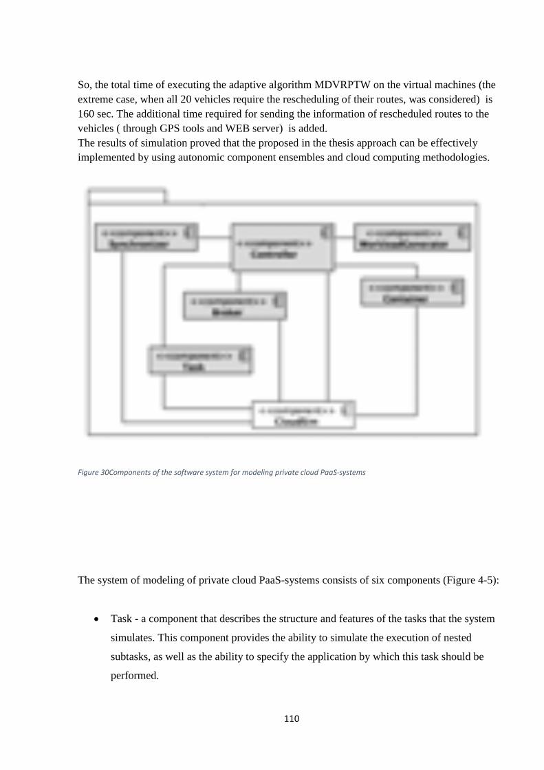
110

So, the total time of executing the adaptive algorithm MDVRPTW on the virtual machines (the extreme case, when all 20 vehicles require the rescheduling of their routes, was considered) is 160 sec. The additional time required for sending the information of rescheduled routes to the vehicles ( through GPS tools and WEB server) is added. The results of simulation proved that the proposed in the thesis approach can be effectively implemented by using autonomic component ensembles and cloud computing methodologies.

Figure 30Components of the software system for modeling private cloud PaaS-systems

The system of modeling of private cloud PaaS-systems consists of six components (Figure 4-5):

• Task - a component that describes the structure and features of the tasks that the system

simulates. This component provides the ability to simulate the execution of nested

subtasks, as well as the ability to specify the application by which this task should be

performed.

111

• Container - a component that provides the functionality of the virtual machine within the

simulation. Provides the ability to simulate the deployment of applications, as well as

managing their lifecycle.

• WorkloadGenerator - a component that generates real-time load during the simulation.

This component provides the periodic addition of tasks to the modeling subsystem of the

simulated system, which allows you to simulate a predictable dynamic load on the

system.

• Synchronizer - component that ensures correct modification of the simulated system

during the simulation run. During simulation, the need for synchronization arises when

simulating a spontaneous load, as well as using a decentralized approach to planning, in

which resource schedulers are responsible for resource scheduling

• Broker - a component that implements the management of the resources of the simulated

system during the simulation. The tasks of this component include the distribution of

virtual machines on the nodes available in the simulated system, the distribution of

applications by virtual machines, the distribution of tasks by applications.

• Controller - a component that prepares the essence of the simulated system based on the

content of the configuration file prepared by the user.

• Cloudlet: this component represents the application service whose complexity is modeled

in CloudSim in terms of the computational requirements.

• CloudCoordinator: this component manages the communication between other

CloudCoordinator services and brokers, and also monitor the internal state of a data

center which will be done periodically in terms of the simulation time.

112

Figure 31 Components CloudSim[45]

The main for modeling the cloud system is the configuration file of the model - JSON document,

which contains a detailed description of the hardware infrastructure of the simulated system, as

well as the simulation scenario. The configuration file consists of two blocks:

• datacenter - contains a description of the infrastructure of the system being

simulated;

• workload - description of the simulation scenario.

The datacenter block describes the physical nodes (hosts block), virtual machines (vms block),

task scheduling algorithms, and application distribution (block brokers). Each described physical

node in the hosts block has a number of attributes:

• quantity - the number of nodes with the described characteristics;

• ram - memory of the node;

• storage - available disk storage;

• bandwidth - network bandwidth;

• CPUs - a list of available processors with the processing power specified in

the millions of processor instructions per second (mips).

113

The description of virtual machines in the vms block has a structure similar to the description of

physical nodes:

• quantity - the number of virtual machines with the characteristics described;

• cpu - the number of required cores;

• size - the size of the image;

• ram - required RAM;

• bandwidth - network bandwidth;

• mips - the required processing power in millions of processor instructions per

second.

The brokers block specifies the paths to the files that contain the scheduling algorithms for tasks

and distribution of applications in the simulated cloud environment. The developed system of

modeling of private cloud PaaS-systems provides the possibility of implementing own

algorithms for managing tasks and distributing applications.

The description of the simulation scenario in the workload block contains a list of tasks for the

simulated system, the number of re-adding tasks to the queue and the time delay before re-

adding tasks. The task description has the following structure:

• quantity - number of tasks with the same description;

• length - the number of processor instructions required to complete the task;

• fileSize - the size of the job file in megabytes;

• outputSize - the size of the result of the task in megabytes;

• app - the application that should perform the task;

• subtasks - an optional block describing the list of tasks that will be added to

the queue after the simulation of the task of the owner is completed.

114

4.3 Chapter IV Summary

Application Of DEECo Framework To MDVRPTW Problem is reviewed and Cloud computing is

described this approaches we use for our dissertation. Payments Pay-as-you-go for consumed

resources of the Google Cloud Platform datacenter are on average 60% less for many compute

workloads than other clouds. Implementation of Autonomic Components Ensembles (ACE) on

Google Cloud Platform (and, in general, on other cloudproviders platforms) shifts most of the

costs from capital expenditures (or buying and installing servers, storage, networking, and related

infrastructure) to an operating expenses model, where customers pay only for usage of these types

of resources.

115

Conclusion and Future Works

As the main goal of MDVRP is reducing the distances and on the basis of reducing distances also

shortening total costs of whole travel, some effective heuristics should be applied to this given

problem. There exist multiple techniques of solving VRP and TSP in exact methods which are

described in this thesis. But with such methods optimal solutions cannot be obtained due too many

constrains and complexity of real life environment. Such constrains as human factor and traffic

congestions are not considered in most heuristics. Earlier in this thesis LNS and ALNS and their

extensions were briefly explained. Both methods have great potential, but anyway there not

enough for implementing of real world transportation problems. However, in general, this given

heuristics work well with partitioning decisions. A number of powerful metaheuristics as Tabu

search and genetic algorithm have also been proposed. But only by adopting and incorporating

many approaches and heuristics we can get desired results. In our dissertation we proposed

heuristics that can get close to optimal solutions. We believe that our approach can help in fields

of logistic applied to our country’s situation in this field.

In our thesis the following items have been studied and developed:

• Theoretical approach that considers uncertainty and stochastic nature of VRP real life

environment in transportation fields

• Mathematical models which define and forecast all of the parameters of the transport

network functioning, such as traffic intensity on all network elements, traffic volumes in

the public transport network, average traffic speeds congestion conditions (congestion

induced delays), have been proposed and developed.

• A set of algorithms and applied tools which combine the application of known algorithms

for searching optimal routes and usage of new technology of autonomous components

ensembles, has been developed. The developed program complex allows users to modify

promptly current routes based on local information and choose the most accessible routes

which reflect local real situation. The complex also allows users to modify routes in

simultaneous and parallel manner without the need to install expensive equipment and

software in vehicles.

• The modification of well-known algorithm ALNS which allows planning of partial routes

by autonomic components (on virtual machines) has been proposed and implemented.

116

• The JSprit framework for modification of the proposed algorithms was used. Based on Java

language this framework allows to conveniently describe and generate required solutions.

• To overcome the shortage of realistic and reliable ways of congestion period estimation

we have a tendency to use the MatSim large-scale agent-based simulation tool. This tool

has permitted us to compose and run complex simulation models that are very close to

the real-world situations.

• Implementation of DEECo model to create dynamic ensembles of vehicles and non-

congested route segments has been proposed and developed in the thesis.

• Extensive use of cloud computing framework allowed us to significantly reduce cost of

calculations; besides cloud computing framework is the most suitable and effective tools

for the methods proposed in the thesis.

The work is of a theoretical and experimental nature. New properties of various routing

problems are obtained, known mathematical models are modified and new mathematical

models are constructed, numerical methods of solution are developed. The developed

methods are implemented as a set of programs. They have shown their effectiveness and can

be used in solving practical problems of large dimension

117

118

References and Literature

1 ) Harnoor K. (2013) Review Paper on Multi-Depot Vehicle Routing Problem by International Journal of Scientific & Engineering Research, Volume 4, Issue 8, August-410 ISSN 2229-5518

2) https://txemainlogisticsworld.wordpress.com

3) Rajesh M, Surya Prakash S, and .Murari Lal M., Traveling Salesman Problem: An Overview of Applications, Formulations, and Solution Approaches 1Management Group, BITS-Pilani 2Department of Management Studies, Indian Institute of Technology Delhi, New Delhi 3Department of Mechanical Engineering, Malviya National Institute of Technology Jaipur, India)

4) Pisinger, D., & Røpke, S. (2010). Large Neighborhood Search. In M. Gendreau (Ed.), Handbook of Metaheuristics (2 ed., pp. 399-420). Springer.

5) Bard J.F., Huang L., Dror M. And Jaillet P. (1995) A branch and cut algorithm for the VRP with satellite facilities

6) Dantzig, G.B.; Fulkerson, D.R. & Johnson, S.M. (1954). Solution of a large-scale traveling salesman problem. Operations Research, Vol. 2, pp.393–410.

7) Martin, G.T. (1966). Solving the traveling salesman problem by integer programming. Working Paper, CEIR, New York.

8) Miliotis, P. (1978). Using cutting planes to solve the symmetric travelling salesman problem. Mathematical Programming, Vol. 15, pp. 177–188.

9) Gomory, R.E. (1963). An algorithm for integer solutions to linear programs. In: Graves RL & Wolfe P (eds). Recent Advances in Mathematical Programming. McGraw-Hill: New York, pp. 269–302.

10) Land, A.H. (1979). The solution of some 100-city traveling salesman problems. Technical report, London School of Economics, London.

11)Applegate, D.L., Bixby, R.E., Chv´atal, V. & Cook, W.J. (2003). Implementing the Dantzig– Fulkerson–Johnson algorithm for large scale traveling salesman problems. Math Program Ser B Vol. 97, pp. 91–153.

12)Applegate, D. L.; Bixby, R. E.; Chvátal, V. & Cook, W. J. (2006), The Traveling Salesman Problem: A Computational Study, Princeton University Press, ISBN 978-0-691-12993-8.

13) Applegate, D.L.; Bixby, R.E.; Chv´atal, V.; Cook, W.J.; Espinoza, D.G.; Goycoolea, M. & Helsgaun, K. (2009). Certification of an optimal TSP tour through 85900 cities. Operations Research Letters., Vol. 37, No. 1, pp. 11–15.

119

14) Laporte, G. & Nobert, Y. (1980). A cutting planes algorithm for the m-salesmen problem. Journal of the Operational Research Society, Vol. 31, pp.1017–23.

15) Arora, S. (1998). Polynomial Time Approximation Schemes for Euclidian Traveling Salesman and Other Geometric Problems, Journal of the ACM, Vol. 45, No. 5, September 1998, pp. 753-782.

16) Dorigo, M. & Gambardella, L.M. (1996). “Ant Colonies for the Traveling Salesman Problem”, University Libre de Bruxelles, Belgium.

17) Johnson D. S., Mcgeoch L. A., And Rothberg E. E.,(1996) ‘‘Asymptotic experimental analysis for the Held-Karp traveling salesman bound,’’ in ‘‘Proceedings 7th ACM SIAM Symp. on Discrete Algorithms,’’ Society for Industrial and Applied Mathematics, Philadelphia York,

18) Chepuri K ., Homem-de-Mello T. Solving the Vehicle Routing Problem with Stochastic Demands using the Cross Entropy Method Department of Industrial, Systems Engineering The Ohio State University, Columbus, OH, USA

19) de Boer, P.T. D.P. Kroese, S. Mannor, and R.Y. Rubinstein. (2005). “A Tutorial on the Cross-Entropy Method.” Annals Of Operations Research 134, 19–67.

20) Horni A, Nagel A,. Axhausen Kay W (2015) The Multi-Agent Transport Simulation MATSim 21) Xinjie Yu · Mitsuo Gen 2010 Introduction to Evolutionary Algorithms ISSN 1619‐5736 22) Bures T, Gerostathopoulos I, HnetynkaP, Keznik J, Kit M.,, Plasil1 F. 2013 DEECo – an Ensemble-Based Component System Technical report No. D3S-TR-2013-02, Version 1.0, February 2013. 23) Bures T, Gerostathopoulos I, HnetynkaP, Keznik J, Kit M.,, Plasil1 F. 2013 DEECo Computational Model – I Rima Al Ali 24) Jsprit - a Java based, open source toolkit for solving rich traveling salesman (TSP) and vehicle routing problems (VRP), from http://jsprit.github.io/

25) Prangishvili A, Shonia O, Rodonaia I, Merabiani A,. (2017) Adaptive Real-World Algorithm of Solving MDVRPTW (Multi Depots Vehicle Routing Planning with Time Windows) Problem. International Journal of Transportation Systems, 2, 1-6

26) Guner Ali R., Murat Alper, Ratna Babu Chinnam. (2012) Dynamic routing under recurrent and non-recurrent congestion using realtime ITS information, Computers & Operations Research 39 358–373

27). Kritzinger S. Doerner K.F., Ttricoire F., Hartl R.F.. (2015), Adaptive search techniques for problems in vehicle routing,Part 1: a survey. Yugoslav Journal of Operations Research 25 Number 1, 3–31

120

28) De Nicola R, Loreti M, Pugliese R., Tiezzi F. (2013)“SCEL- a Language for Autonomic Computing”. ASCENS project , Technical report, January

29) Prangishvili A., Shonia O., Rodonaia I., Mousa M.. (2014) Formal verification in autonomic-component ensembles, WSEAS / NAUN International Conferences, Salerno, Italy,

30). Rodonaia I., Merabiani A. (2016) Real-world applications of the vehicle routing problem in Georgia., Journal Technical Science & Technologies (JTST), is. (2) 41 -44 November,

31) Pillac, V., Gueret, Ch., & Medaglia, A. (2011). Dynamic Vehicle Routing Problems: State of the art and Prospects. Technical Report 10/4/AUTO.. HAL Id: hal-00623474, https://hal. archives-ouvertes.fr/hal-00623474,2011

32) Kok, A.L., Hans, E.W., & Schutten, J.M.J. (2013) Vehicle routing under time-dependent travel times: the impact of congestion avoidance. Operational Methods for Production and Logistics, University of Twente, P.O. Box 217, 7500AE, Enschede, Netherlands,.

33) Lutz, R. (2014). Adaptive Large Neighborhood Search. Bachelor thesis at Ulm University

34) http://searchcloudcomputing.techtarget.com/definition/cloud-computing

35) Gutin G. and Karapetyan. D. Local search heuristics for the multidimensional

assignment problem. In Proc. Golumbic Festschrift, volume 5420, pages 100–115. 2009.

36 ) Holland J.H. (1975)Adaptation in Natural and Artificial Systems. The University of Michigan Press,

37) De Jong K. ( 1975)An analysis of the behavior of a class of genetic adaptive systems. Doctoral dissertation. – University of Michigan, Ann Arbor. – University Microfilms No. 76-9381. –.

38) Agentenbasiertes Verkehrsmodell Vorarlberg Autoren: DDI(FH) Gernot Lenz, Dr. Christian Rudloff, Dr. Michael Ulm AIT Austrian Institute of Technology GmbH Mobility Department | Dynamic Transportation Systems

39) Avery S, Oswald T.; Colin M. MacLeod; Maclyn McCarty (1944-02-01). "Studies on the Chemical Nature of the Substance Inducing Transformation of Pneumococcal Types: Induction of Transformation by a Desoxyribonucleic Acid Fraction Isolated from Pneumococcus Type III". Journal of Experimental Medicine. 79 (2): 137–158. doi:10.1084/jem.79.2.137. PMC 2135445Freely accessible. PMID 19871359. Archived from the original on 7 October 2008. Retrieved 2008-09-29.

40) Bresciani P., Giorgini P., Giunchiglia F., Mylopoulos, J. and Perini. A. (2004): An Agent-Oriented Software Development Methodology. Autonomous Agents and Multi- Agent Systems. 8, 3, 2004.

121

41) Calheiros RN, Ranjan R, Beloglazov A, De Rose CA, Buyya R (2011). "CloudSim: a toolkit for modeling and simulation of cloud computing environments and evaluation of resource provisioning algorithms." . Software: Practice and Experience. 41 (1): 23–50.

42) Sá, Thiago Teixeira; Calheiros, Rodrigo N.; Gomes., Danielo G. (2014). "CloudReports: An Extensible Simulation Tool for Energy-Aware Cloud Computing Environments.". In Cloud Computing, Springer International Publishing: 127–142.

43) Gustedt, J. Experimental methodologies for large-scale systems: a survey / J. Gustedt, E. Jeannot, M. Quinson // Parallel Process. Lett. — World Scientific, 2009. — Vol. 19. — P. 399–418. 44) Jararweh, Y. TeachCloud (2012): a cloud computing educational toolkit / Y. Jararweh et al. // Int. J. Cloud Comput. 2012. — InderScience Publ.,. — Vol. 2. — P. 237–257. 45) http://cloud-simulation-frameworks.wikispaces.asu.edu 46) Rai R K, Balmer M., Rieser R. Axhausen Kay W. (2007) Capturing Human Activity Spaces: New Geometries · Transportation Research Record Journal of the Transportation Research Board 47) Lehu´ed´e F and P´eton´ Ecole O., An Adaptive Large Neighborhood Search for the Pickup and Delivery Problem with Transfers Renaud Masson, des Mines de Nantes/IRCCyN 4 rue Alfred Kastler, F-44307 Nantes, France 48) Solomon M. M.. (1987) Algorithms for the Vehicle Routing and Scheduling Problems with Time Window Constraints. Operations Research,35(2):254–265, 1987. 49) Desrosiers J., Dumas Y., Solomon M. M., and Soumis F.. (1995) Time constrained routing and scheduling. In M. O. Ball, T. L. Magnanti,C. L. Monma, and G. L. Nemhauser, editors, Handbooks in Operations Research and Management Science, chapter 8, pages 35–139. Elsevier Science Publishers, Amsterdam, The Netherlands,. 50) Br¨aysy O. and Gendreau M.( 2005). Vehicle routing problem with time windows, part I: Route construction and local search algorithms. Transportation Science, 39(1):104–118,. 51) Eberhardt S. P., Duad T., Kerns A., Brown T. X., Thakoor A. P., (1991) Competitive Neural Architecture for Hardware Solution to the Assignment Problem, Neural Network, 4(4), 431-442,. 52) Dyckhoff H., Scheithauer G., and Scheithauer J. (1997). Cutting and Packing (C&P). In M. Dell’Amico, F. Maffioli, and S. Martello, editors, Annotated Bibliographies in Combinatorial

122

Optimization. John Wiley & Sons, Chichester,. 53) Bertsimas D. J. and van Ryzin G. J..(1993) Stochastic and dynamic vehicle routing with general interarrival and service time distributions. Advances in Applied Probability, 25:947–978,. 54) Fuglestvedt J., Bernstein T., Myhre G. Rypdal K and Skeie R. (2008) Climate forcing from the transport sectors. Proceedings of the National Academy of Sciences, 105(2):454-458, 55) Lenstra J. and Rinnooy Kan H.. (1981) Complexity of vehicle routing and scheduling problems Networks, 11(2):221-227, 56) Golden B., Wasil E., Kelly J and Chao I. (1998) The Impact of Metaheuristics on solving the Vehicle Routing Problem: Algorithms Problem Sets and Computational Results. In T.G. Crainic and G Laporte, editors, Fleet Management and Logistics, Centre for research on Transportation pages 33-56 Springer US, 57) Altinel I.K. and Onkan T.(2005). A new enhancement of the Clarke and Wright savings heuristics for the capacitated vehicle problem Journal of the Operational Research Society, 56:954-961. 58) Toth P. and Tramontani A.(2008) An Integer linear programing local search of Capacitated Vehicle Routing Problems In B.Golden, S Raghavan E.Wasil, editors, The vehicle routing problem: Latest Advances and New Chalanges, volume 43 of Operations Research/Computer Science Interface, pages 143-169 Springer US, 59) Christofides N. and Beasley J (1984). The Period routing problem. Neworks, 14(2):237-256, 60) Potvin J., and Rousseau J.,(1993) A parallel route building algorithm for the vehicle routing and scheduling problem with time windows. European Journal of Operational research, 66(3):331-340,. 61) Vidal T., Crainic T., Gendraeu M., Lahrichi N. and Rei W. (2012)A hybrid genetic algorithm for multi-depot and perdiodic vehicle routing problems Operations Research, 60(3): 611-624, 62) Hadjiconstantinou E. and Baldacci R.. (1998) A Multi-Depot Vehicle Routing Problem arising in the utilities sector. Journal of the operational Research Sosiety, 49(12):1239-1248, 63) Dror M., Laporte G. and Truedeau P., (1994) Vehicle routing with split deliveries. Discrete Apllied Mathematics, 50 (3):239-254, 64) Gutin G., Yeo A. and Zverovich A., (2002), Traveling salesman should not be greedy: domination analysis of greedy-type heuristics for the TSP. Discrete Applied Mathematics 117 81-86.

123

65) Bang-Jensen J., Gutin G. and Yeo A. (2004), When the greedy algorithm fails. Discrete Optimization is. (1) 121-127. 66) Cormen, Leiserson, and Rivest (1990) Introduction to Algorithms, Chapter 17 "Greedy Algorithms" p. 329.

67) Cormen, Leiserson, Rivest, and Stein (2001) Introduction to Algorithms , Chapter 16 "Greedy Algorithms".

68) Lin, Shen; Kernighan, B. W. (1973). "An Effective Heuristic Algorithm for the Traveling-Salesman Problem". Operations Research. 21 (2): 498–516. doi:10.1287/opre.21.2.498. 69) K. Helsgaun .(2000) "An Effective Implementation of the Lin-Kernighan Traveling Salesman Heuristic". European Journal of Operational Research. 126 (1): 106–130. 70) Glover F. (1986) "Future Paths for Integer Programming and Links to Artificial Intelligence". Computers and Operations Research. 13 (5): 533–549 71) Khachaturyan, A.; Semenovskaya, S.; Vainshtein, (1979).. "Statistical-Thermodynamic Approach to Determination of Structure Amplitude Phases". Sov.Phys. Crystallography. 24 (5): 519–524. 72) Granville, V.; Krivanek, M.; Rasson, J.-P. (1994). "Simulated annealing: A proof of convergence". IEEE Transactions on Pattern Analysis and Machine Intelligence. 16 (6): 652–656. 73) Little, John D. C.; Murty, Katta G.; Sweeney, Dura W.; Karel, Caroline (1963). "An algorithm for the traveling salesman problem" . Operations Research. 11 (6): 972–989. 1963 74) Bader A, David A.; Hart, William E.; Phillips, Cynthia A. (2004). "Parallel Algorithm Design for Branch and Bound" (PDF). In Greenberg, H. J. Tutorials on Emerging Methodologies and Applications in Operations Research. Kluwer Academic Press. 75) Charon I., Hudry H. The noising methods. A survey. In: Ribeiro C. C., Hansen P. (1998.) Meta-heuristics: Advances and Trends in Local Search Paradigms for Optimization. Boston: Kluwer. Acad. Publ.,. P. 245–262. 76) Merabiani A. (2017) Application of DEECO Framework to MDVRPTW Problem. “Automated Control Systems” (Online-Journal) is. N1(23)

77) Shaw P. (1998) Using constraint programming and local search methods to solve vehicle routing problems. In CP-98 (Fourth International Conference on Principles and Practice of Constraint Programming), volume 1520 of Lecture Notes in “Computer Science”, pages 417–431,.