iot sensor swarm foragricultural microclimate measurement
TRANSCRIPT
IoT Sensor Swarm for AgriculturalMicroclimate Measurement
DIPLOMARBEIT
zur Erlangung des akademischen Grades
Diplom-Ingenieur
im Rahmen des Studiums
Technische Informatik
eingereicht von
Thomas Puchinger, BScMatrikelnummer 0928809
an der Fakultät für Informatik
der Technischen Universität Wien
Betreuung: Univ.Prof. Dipl.-Ing. Dr.rer.nat. Radu GrosuMitwirkung: Proj.Ass. Dipl.-Ing. BSc Christian Hirsch
Wien, 8. Dezember 2020Thomas Puchinger Radu Grosu
Technische Universität WienA-1040 Wien Karlsplatz 13 Tel. +43-1-58801-0 www.tuwien.at


IoT Sensor Swarm for AgriculturalMicroclimate Measurement
DIPLOMA THESIS
submitted in partial fulfillment of the requirements for the degree of
Diplom-Ingenieur
in
Computer Engineering
by
Thomas Puchinger, BScRegistration Number 0928809
to the Faculty of Informatics
at the TU Wien
Advisor: Univ.Prof. Dipl.-Ing. Dr.rer.nat. Radu GrosuAssistance: Proj.Ass. Dipl.-Ing. BSc Christian Hirsch
Vienna, 8th December, 2020Thomas Puchinger Radu Grosu
Technische Universität WienA-1040 Wien Karlsplatz 13 Tel. +43-1-58801-0 www.tuwien.at


Erklärung zur Verfassung derArbeit
Thomas Puchinger, BSc
Hiermit erkläre ich, dass ich diese Arbeit selbständig verfasst habe, dass ich die verwen-deten Quellen und Hilfsmittel vollständig angegeben habe und dass ich die Stellen derArbeit – einschließlich Tabellen, Karten und Abbildungen –, die anderen Werken oderdem Internet im Wortlaut oder dem Sinn nach entnommen sind, auf jeden Fall unterAngabe der Quelle als Entlehnung kenntlich gemacht habe.
Wien, 8. Dezember 2020Thomas Puchinger
v


Danksagung
Dem Leiter des Forschungsbereiches Cyber Physical Systems Univ.Prof. Dipl.-Ing. Dr. rernat. Radu Grosu gilt mein aufrichtiger Dank - für die Betreuung und Begutachtung dieserArbeit. Meinen KollegInnen der TU Wien, Dipl.-Ing. Christian Hirsch BSc, Dipl.-Ing.Michael Platzer und Ing. Leo Mayerhofer für ihren fachlichen Rat und ihre kompetenteUnterstützung, sowie Viktoria Vasalik, die sich mit ihrer Englischkompetenz eingebrachthat und mir bei teils schwierigen Übersetzungen zur Seite stand.
Für die mentale Unterstützung danke ich meiner Familie. Meiner Frau Tamara für dasGegenlesen der Thesis und ihren Rat sowie meinen Eltern für ihre Unterstützung, sodasses mir möglich war, meine Studien abzuschließen.
Stetige Motivation und fachliches Feedback waren mir eine große Stütze, danke hierfürfür die langjährige Freundschaft, Alexander, Bernhard und Christoph.
vii


Acknowledgements
A special “Thank you” to the Head of the Research Unit Cyber Physical Systems,Univ.Prof. Dipl.-Ing. Dr.rer.nat. Radu Grosu, for supervising this thesis. I am gratefulto my colleagues at the TU Wien, Dipl.-Ing. Christian Hirsch BSc, Dipl.-Ing. MichaelPlatzer and Ing. Leo Mayerhofer for their professional advice and competent support.Thanks to Viktoria Vasalik as well, who stood by my side with her language skills andhelped translate difficult phrases into English. I am grateful to my family for the mentalsupport, to my wife, Tamara, for reading my thesis and her constructive criticism and tomy parents, who helped me finish my studies.
Constant motivation and professional feedback were a great support for me, thanks forthe long friendship, Alexander, Bernhard and Christoph.
ix

Kurzfassung
Mit dem Internet verbundene vernetze Sensor Systeme, auch Internet of Things (IoT)genannt, haben sich in den letzten Jahren rasch weiterentwickelt. Dadurch sind viele neueAnwendungsfälle und Einsatzmöglichkeiten entstanden und sie entstehen kontinuierlich.Damit die heutige Landwirtschaft kostendeckend wirtschaften kann, wird es immernotwendiger, Agrarflächen noch genauer und verteilter zu messen. Grund hierfür sinddie steigenden Kosten für Löhne, Material und Verbrauchsmittel. Aufgrund des starkenWettbewerbes stagnieren jedoch die Marktpreise. Um die notwendigen Arbeitsschritte imPflanzenschutz genauer planen zu können, sind genaue Messwerte der Umwelt erforderlich.Zwei hierfür relevante Messwerte sind die Blattfeuchte und der Ultraviolet Radiation (UV)Wert. Ziel dieser Arbeit ist es, einen Prototyp zu entwickeln, der diese beiden Messwertesensorisch erfasst. Diese Messwerte sollen ins Internet übertragen werden, dazu sindder Entwurf und Aufbau eines entsprechenden Sensor Netzwerkes, auch Sensor Swarmgenannt, erforderlich. Während des gesamten Entwicklungsprozesses wird darauf geachtet,die Kosten für den Sensor so gering wie möglich und den Stromverbrauch niedrig zuhalten, um die Autarkheit des Sensors zu gewährleisten.
Der durchgeführte Feldtest zeigt, dass der selbst gebaute Sensor autark arbeiten kannund die Zuverlässigkeit bei mindestens 87 Prozent liegt. Die Kosten für einen Sensorliegen unter 150 e pro Stück und unterschreiten damit die Erwerbskosten kommerziellerhältlicher Produkte. Auch wenn vor einer potenziellen Markteinführung des Systemsnoch Hürden genommen werden müssten, konnte durch diese Arbeit nachgewiesen werden,dass das geschaffene Sensor Netzwerk sich auch in der Praxis bewährt hat.
xi

Abstract
Networked sensor systems connected to the Internet, also called Internet of Things (IoT),have rapidly developed in the past few years. This has created and is continuing tocreate many new applications and possible use cases. To enable today’s agriculturalorganizations to cover their costs, more accurate and distributed measurements of theagricultural land are necessary. The reason for this are the rising salaries and the risingcosts of materials and consumables. However, the market prices of agricultural productsare stagnating due to strong competition. To be able to plan the necessary steps in plantprotection more precisely, accurate measurements of the environment are required. Tworelevant measured values are leaf wetness and UV value. The aim of this thesis is todevelop a prototype that measures these two values. These measured values are to betransmitted to the Internet; to do this, a corresponding sensor network, also called sensorswarm, has to be designed and constructed. Throughout the development process, thecosts of the sensor and the power consumption are kept as low as possible to ensure theself-sufficiency of the sensor. The field test carried out shows that the self-built sensorcan operate autonomously and the reliability is at least 87 percent. The cost of a sensoris less than e150 per unit, which is less than the purchase cost of commercially availableproducts. Even if a potential market launch would prove difficult in the beginning, thisthesis establishes that the created sensor network has proven itself in practice.
xiii

Contents
Kurzfassung xi
Abstract xiii
Contents xv
1 Introduction 11.1 Problem Description and Motivation . . . . . . . . . . . . . . . . . . . . 11.2 Aim of This Work . . . . . . . . . . . . . . . . . . . . . . . . . . . . . 21.3 Methodological Approach . . . . . . . . . . . . . . . . . . . . . . . . . 31.4 Structure of This Work . . . . . . . . . . . . . . . . . . . . . . . . . . 3
2 State of the Art 52.1 Transmission Methods . . . . . . . . . . . . . . . . . . . . . . . . . . . 5
2.1.1 Network Topologies . . . . . . . . . . . . . . . . . . . . . . . . 62.1.2 Wired Network . . . . . . . . . . . . . . . . . . . . . . . . . . . 72.1.3 Wireless Network . . . . . . . . . . . . . . . . . . . . . . . . . . 8
2.2 OSI Model . . . . . . . . . . . . . . . . . . . . . . . . . . . . . . . . . . 82.3 Physical and Data Link Layer . . . . . . . . . . . . . . . . . . . . . . . 8
2.3.1 Institute of Electrical and Electronics Engineers (IEEE) 802.3 . 92.3.2 IEEE 802.15.4 . . . . . . . . . . . . . . . . . . . . . . . . . . . 9
2.4 Network Layer . . . . . . . . . . . . . . . . . . . . . . . . . . . . . . . 132.4.1 IPv6 over Low power Wireless Personal Area Network (6LoWPAN) 13
2.5 Transport Layer . . . . . . . . . . . . . . . . . . . . . . . . . . . . . . 142.6 Session, Presentation and Application Layer . . . . . . . . . . . . . . . 14
2.6.1 Hypertext Transfer Protocol (HTTP) . . . . . . . . . . . . . . 142.6.2 Constrained Application Protocol (CoAP) . . . . . . . . . . . . 152.6.3 Message Queuing Telemetry Transport (MQTT) . . . . . . . . 15
2.7 Wireless Technologies for IoT . . . . . . . . . . . . . . . . . . . . . . . 162.7.1 Thread . . . . . . . . . . . . . . . . . . . . . . . . . . . . . . . 16
OpenThread . . . . . . . . . . . . . . . . . . . . . . . . . . . . 19MbedOS . . . . . . . . . . . . . . . . . . . . . . . . . . . . . . . 19
2.7.2 Bluetooth . . . . . . . . . . . . . . . . . . . . . . . . . . . . . . 19
xv

Bluetooth Low Energy (BLE) . . . . . . . . . . . . . . . . . . . 192.7.3 Bluetooth Mesh . . . . . . . . . . . . . . . . . . . . . . . . . . . 20
2.8 Sensors for Microclimate Measurement . . . . . . . . . . . . . . . . . . . 212.8.1 Soil Moisture . . . . . . . . . . . . . . . . . . . . . . . . . . . . . 212.8.2 Leaf Wetness . . . . . . . . . . . . . . . . . . . . . . . . . . . . 232.8.3 UV Radiation . . . . . . . . . . . . . . . . . . . . . . . . . . . . 25
Change in Temperature (Bolometer) . . . . . . . . . . . . . . . 25External Photoelectric Effect . . . . . . . . . . . . . . . . . . . 25Internal Photoelectric Effect . . . . . . . . . . . . . . . . . . . . 26
2.9 Concepts for Microclimate In-Field Measurement . . . . . . . . . . . . 272.9.1 VitiMeteo Plasmopara . . . . . . . . . . . . . . . . . . . . . . . 272.9.2 Adcon . . . . . . . . . . . . . . . . . . . . . . . . . . . . . . . . 282.9.3 Metos . . . . . . . . . . . . . . . . . . . . . . . . . . . . . . . . 282.9.4 Davis . . . . . . . . . . . . . . . . . . . . . . . . . . . . . . . . 292.9.5 Libelium . . . . . . . . . . . . . . . . . . . . . . . . . . . . . . . 30
2.10 Microclimate Measurement With Satellites . . . . . . . . . . . . . . . 32
3 Requirements and Design Decision 353.1 Hardware Requirements . . . . . . . . . . . . . . . . . . . . . . . . . . 353.2 Software Requirements . . . . . . . . . . . . . . . . . . . . . . . . . . . 373.3 Measurement Requirements . . . . . . . . . . . . . . . . . . . . . . . . 373.4 Comparison . . . . . . . . . . . . . . . . . . . . . . . . . . . . . . . . . 373.5 Design Decision . . . . . . . . . . . . . . . . . . . . . . . . . . . . . . . 39
4 System Design 414.1 LWS . . . . . . . . . . . . . . . . . . . . . . . . . . . . . . . . . . . . . . 414.2 UV Sensor . . . . . . . . . . . . . . . . . . . . . . . . . . . . . . . . . . 454.3 Data Transmission . . . . . . . . . . . . . . . . . . . . . . . . . . . . . 46
4.3.1 Data Storage . . . . . . . . . . . . . . . . . . . . . . . . . . . . 504.4 System on Chip . . . . . . . . . . . . . . . . . . . . . . . . . . . . . . . . 514.5 Power Management . . . . . . . . . . . . . . . . . . . . . . . . . . . . . 52
4.5.1 Circuits for Power Management . . . . . . . . . . . . . . . . . . 53Variant 1: Dual Input Charger IC . . . . . . . . . . . . . . . . 54Variant 2: Power Mux With a Single Input Charger IC . . . . 54Variant 3: Single Input Charger IC . . . . . . . . . . . . . . . . 55
4.5.2 Design Decision . . . . . . . . . . . . . . . . . . . . . . . . . . . 564.5.3 Approximate Power Consumption . . . . . . . . . . . . . . . . 564.5.4 Batteries . . . . . . . . . . . . . . . . . . . . . . . . . . . . . . 584.5.5 Solar Panel Dimensioning . . . . . . . . . . . . . . . . . . . . . 59
4.6 2.4 GHz Antenna . . . . . . . . . . . . . . . . . . . . . . . . . . . . . . 60
5 Hardware Implementation 615.1 nRF52840 SoC Circuit . . . . . . . . . . . . . . . . . . . . . . . . . . . . 615.2 2.4 GHz Antenna . . . . . . . . . . . . . . . . . . . . . . . . . . . . . . . 61
5.3 Power Management . . . . . . . . . . . . . . . . . . . . . . . . . . . . . 635.3.1 Power Mux . . . . . . . . . . . . . . . . . . . . . . . . . . . . . 645.3.2 Battery Charger . . . . . . . . . . . . . . . . . . . . . . . . . . 65
5.4 Leaf Wetness Measurement . . . . . . . . . . . . . . . . . . . . . . . . 675.5 UV Measurement Circuit . . . . . . . . . . . . . . . . . . . . . . . . . 705.6 Finished Board . . . . . . . . . . . . . . . . . . . . . . . . . . . . . . . . 71
6 Software Implementation 736.1 Sensor Node . . . . . . . . . . . . . . . . . . . . . . . . . . . . . . . . . 73
6.1.1 Data Storage . . . . . . . . . . . . . . . . . . . . . . . . . . . . 746.1.2 Analog to Digital Converter (ADC) . . . . . . . . . . . . . . . 756.1.3 Inter-Integrated Circuit (I2C) . . . . . . . . . . . . . . . . . . . 756.1.4 Pulse Width Modulation (PWM) . . . . . . . . . . . . . . . . . 766.1.5 WDT . . . . . . . . . . . . . . . . . . . . . . . . . . . . . . . . 766.1.6 VEML6070 . . . . . . . . . . . . . . . . . . . . . . . . . . . . . 766.1.7 BQ25895 . . . . . . . . . . . . . . . . . . . . . . . . . . . . . . 766.1.8 Leaf Wetness State Machine . . . . . . . . . . . . . . . . . . . . 776.1.9 Main Program State Machines . . . . . . . . . . . . . . . . . . 78
6.2 Relay Node . . . . . . . . . . . . . . . . . . . . . . . . . . . . . . . . . 796.2.1 Data Storage . . . . . . . . . . . . . . . . . . . . . . . . . . . . 796.2.2 Bluetooth . . . . . . . . . . . . . . . . . . . . . . . . . . . . . . 806.2.3 State Machine . . . . . . . . . . . . . . . . . . . . . . . . . . . 80
6.3 Raspberry Pi as Fog Device . . . . . . . . . . . . . . . . . . . . . . . . 806.4 Time Synchronization . . . . . . . . . . . . . . . . . . . . . . . . . . . . 81
6.4.1 Forward Only Method . . . . . . . . . . . . . . . . . . . . . . . . 816.4.2 Relay Buffered Method . . . . . . . . . . . . . . . . . . . . . . . . 816.4.3 Fog Request Method . . . . . . . . . . . . . . . . . . . . . . . . 82
6.5 OpenThread Mesh Network . . . . . . . . . . . . . . . . . . . . . . . . 826.5.1 Commissioning . . . . . . . . . . . . . . . . . . . . . . . . . . . 826.5.2 CoAP . . . . . . . . . . . . . . . . . . . . . . . . . . . . . . . . 83
7 Validation 857.1 Leaf Wetness Sensor (LWS) Area Evaluation . . . . . . . . . . . . . . 85
7.1.1 Comparison of Different PCB Tracks . . . . . . . . . . . . . . . 857.1.2 Relationship of Leaf Wetness to Digital Value . . . . . . . . . . . 917.1.3 Calibration . . . . . . . . . . . . . . . . . . . . . . . . . . . . . . 917.1.4 Comparison to Existing Sensors . . . . . . . . . . . . . . . . . . 94
7.2 Antenna . . . . . . . . . . . . . . . . . . . . . . . . . . . . . . . . . . . 947.3 Power Management . . . . . . . . . . . . . . . . . . . . . . . . . . . . . 947.4 Expenditure on the Board . . . . . . . . . . . . . . . . . . . . . . . . . 987.5 Field Test . . . . . . . . . . . . . . . . . . . . . . . . . . . . . . . . . . 98
7.5.1 Power Consumption . . . . . . . . . . . . . . . . . . . . . . . . 997.5.2 Reliability . . . . . . . . . . . . . . . . . . . . . . . . . . . . . . 100
8 Conclusion 1038.1 Outlook and Further Tasks . . . . . . . . . . . . . . . . . . . . . . . . 103
8.1.1 Sensor Manufacturing . . . . . . . . . . . . . . . . . . . . . . . 1038.1.2 Power Consumption Optimization . . . . . . . . . . . . . . . . 1048.1.3 Increase Reliability . . . . . . . . . . . . . . . . . . . . . . . . . 104
9 Appendix 105
List of Figures 109Acronyms . . . . . . . . . . . . . . . . . . . . . . . . . . . . . . . . . . . . . 113
List of Tables 119
Bibliography 121

CHAPTER 1Introduction
This chapter describes the problem and explains the motivation behind the aim to buildan agricultural sensor swarm for microclimate measurements.
1.1 Problem Description and MotivationToday, the number of devices that are able to transfer data over networks keeps increasing[LL15]. This system of different devices that are connected together to share data is calledInternet of Things (IoT) and it is present, for example, in households, in the entertainmentand mobility sectors. The aim is to exchange data, e.g. weather measurements, in orderto make decisions, create statistical evaluations or to take remote actions. Such systemscan also be used in agriculture to provide farmers with measured data so that they canmake their spraying and irrigation systems more intelligent and can detect diseases easier[MPB+16]. The following parameters are relevant to disease detection in agriculturalmicroclimate systems [HRG18]:
• Temperature
• Humidity
• Solar radiation
• Color of the leaves and the berries
• Water content of the berries
• Raindrops on the berries
• Ripeness of the berries
1

1. Introduction
Table 1.1: Wavelengths of the different UV types.
Type low Value high ValueUltraviolet C (UVC) 200nm 280nmUltraviolet B (UVB) 280nm 320nmUltraviolet A (UVA) 320nm 400nm
visible light 400nm 750nm
The leaf wetness describes how wet or dry the surface of a leaf is. Based on this value, adisease warning system can alert the farmer to possible infections [MFP+16]. UltravioletRadiation (UV) is an electromagnetic radiation, which has too short a wavelength to beseen by humans. Artificial UV light can be created by mercury vapour lamps, back lightor UV Light Emitting Diodes (LEDs). Table 1.1 lists the different types of UV light andtheir respective wavelengths. The UV light affects the photosynthesis and is therefore ofinterest to the farmer [KBD+99]. First of all, these measured values are collected over aperiod of years and then models are created. Farmers are then provided with informationthat was obtained on the basis of these models and current measured values. Vitimeteo[Vit] is a model well known and much used by winemakers. It calculates the life cycle ofthe Plasmopara viticola, which is a disease of the grapevine [BKK+08] and can causesignificant economic damages.
1.2 Aim of This WorkTo create disease models, as much data as possible is needed. The aim of this work isto collect the data with the help of a sensor swarm. This swarm consists of a networkin which the sensors can exchange messages and are able to store the measurementson a server in the cloud. The sensors should be distributed on a field, vineyard ororchard where no infrastructure is given, i.e. there is no electricity, no buildings and noInternet connection via cable available. Therefore, outdoor installation must be possible.The swarm network should contain sensors that measure the leaf wetness and the UVradiation.
2

1.3. Methodological Approach
1.3 Methodological ApproachThe first step is to read the relevant literature and compare the prevailing transmissionmethods and protocols. Then we will compare the existing agricultural microclimatemeasurement systems with respect to the technical function of weather stations, LeafWetness Sensor (LWS) and UV sensors. Based on this comparison and our definedrequirements, we will choose an existing system or a combination of different systems, orwe will develop our own system from zero. Different data flows will be evaluated andcompared, this includes the testing of different transmission methods, e.g. Bluetooth andThread. The sensitivity of different LWSs will be evaluated, the best one then selected forthe prototypes. After finishing the hardware and software development of the prototypes,we will test them and solve problems that arise. After a problem-free indoor test, thesensors will be mounted in the field for testing. If problems occur, the tests will bestopped until the equipment is fixed. At the end of the tests, the collected data will beevaluated.
1.4 Structure of This WorkAfter the Introduction, Chapter Two gives an overview of state-of-the-art techniquesfor wired and wireless data transmission. In addition, existing systems and methodsfor measuring the values related to microclimate in agriculture are reviewed. ChapterThree specifies our requirements for an agricultural microclimate measurement systemand describes our resulting decision for an existing system, a combination of systems,or whether we will develop our own system from zero. Chapter Four describes thedesign of the system. Chapter Five explains the hardware and Chapter Six the softwareimplementation. In Chapter Seven we evaluate the measured data. Chapter Eightsummarizes the implementation, evaluation and the encountered problems. It alsopresents the results we have reached and future tasks.
3


CHAPTER 2State of the Art
This chapter presents existing methods to measure microclimate. Innovations of the pastfew years have improved the techniques and with the help of IoT sensor swarms, whichconsist of many individual sensors, measuring is more reliable [TGL+07]. The protocolsand standards to build such networks are constantly evolving [KK19]. Existing conceptsand standards for transmitting data over networks are studied and compared at thebeginning of this chapter.To simplify the usage of System on Chips (SoCs) in IoT applications, the manufacturersprovide chips with built-in wireless (e.g. Bluetooth Low Energy (BLE), Zigbee, Thread,802.15.4, Near Field Communication (NFC)) and wired technologies. They also providesoftware stacks for these mesh networks. This decreases the time necessary for thedevelopment of new devices for mesh networks. Unfortunately, most of the softwarestacks are closed-source, which means that the developer does not know what the codelooks like and cannot modify it either. To go around this problem, the developer coulduse one of different open-source Real Time Operating Systems (RTOSs).
2.1 Transmission Methods
In principle, there are three ways to transmit data: wired, wireless and optical. HimanshuJha studies and compares wired, wireless and optical networks in his Journal [Jha17].From this study we extracted the properties that are important for our agricultural sensornetwork and compared these in Table 2.1. For our purpose, throughput and latency arenot relevant - because the arrival of the data is not time-dependent. On the other hand,mobility is very important.
5

2. State of the Art
Table 2.1: Comparison of wired and wireless networks [Jha17].
Properties Wired Wireless OpticalLatency medium high low
Throughput medium low highMobility limited not limited limited
(a) (b) (c)
(d) (e) (f)
Figure 2.1: Different Network Topologies, where the lines illustrate the possible commu-nication paths. The connected nodes can build a Line (a), Mesh (b), Ring (c), Star (d),Bus (e) or a Tree (f).
2.1.1 Network Topologies
For the construction of sensor networks, there are different topologies available and theyare illustrated in Figure 2.1. K. Pandya [Pan13] describes the different topologies andtheir advantages and disadvantages, which are listed below.
Line: In this topology each node can have two neighbors at the most. It supports longdistances, but the disadvantage is that if one node fails, the whole chain is interrupted.
Mesh: In a Mesh it is possible that each node communicates with every other node.Therefore, the network can adapt its routing if a node fails. It also supports long distances,by building a chain. The disadvantages are that the routing through the network can getcomplex and that the setup and maintenance is more time-consuming than that of theother topologies.
Ring: In a Ring network each node has exactly two neighbors and therefore each nodecan be accessed from two sides. This is important if, for example, one path is damaged.The disadvantages are the expensive and difficult installation and the detection of afaulty node.
6

2.1. Transmission Methods
Table 2.2: Comparison of protocols that define the physical layer for wired networks.
Protocol Cable Speed TopologyEthernet Twisted Pair, Fiber 10 Mbps Bus, StarFast Ethernet Twisted Pair, Fiber 100 Mbps Star, Mesh1-Wire Twisted Pair 16.3 kbps BusRS-485 Twisted Pair 10 Mbps Bus
Star: In a Star topology all nodes in the network are connected to the central hub. Thishub is responsible for routing the data packets to the destination. The disadvantages arethat the central hub is a Single Point of Failure (SPOF) and that the reachable distanceis limited.
Bus: In a Bus topology a single cable is needed to connect all nodes. Therefore, it isreliable in small networks and requires the least amount of cable. To enlarge the network,only the bus cable has to be extended. The disadvantages are that the sending nodes caninterrupt each other and so they use a lot of bandwidth and each additional connectednode weakens the electric signal.
Tree: The Tree topology is a nested star topology. The hubs can have other hubsconnected to them. The installation of the network is well-ordered and thanks to this, afaulty node can be found by following the traces. The disadvantages are that a failure inthe central hub brings the whole network to a halt and more cabling is required comparedto the Bus topology.
2.1.2 Wired Network
In wired networks, information is transmitted through a solid medium, e.g. copperor glass fiber. To set up a wired network, the topology has to be known in advance.Wired networks are not prone to interferences, they support high speeds (up to 1 Gbit/s)and the possible distances are long [KM14]. In Table 2.2 different protocols for wirednetworks are compared. The Ethernet standard (IEEE 802.3) has many extensions, e.g.Fast Ethernet (IEEE 802.3u) [IEEb]. With the help of Shortest Path Bridging (SPF)[AAB+10], which is specified in IEEE 802.1aq, all routes in an Ethernet network canbe used. This way, a mesh network can be created. 1-Wire [Awt97] describes a serialprotocol from the company Dallas Semiconductor. It only needs data and a groundline. It is used, for example, in home automation [Ste16] and agriculture [Awt98] tomeasure temperature or humidity. RS-485 (EIA-485) [cco99] is defined by the ElectronicIndustries Alliance (EIA), the differential signaling over twisted pair cables improves therobustness towards interferences. Therefore, it can be used over long distances [cco99].
7

2. State of the Art
2.1.3 Wireless Network
In wireless communication, information is transmitted through electromagnetic waves.Wireless sensors can be added to, moved within and removed from the network with lesseffort than in the case of wired networks because there is no cabling necessary. Therefore,wireless sensor networks have recently been used in more and more applications [PDHM14].Standardization organizations are trying to avoid problems with interoperability betweenapplications, by defining unique standards.
These standards try to meet requirements of low power consumption, low latency, highreliability, scalability and security. Mostly, they define a unique Physical, Data Link,Network and Application Layer. Some important organizations and standards are pre-sented below.The Institute of Electrical and Electronics Engineers Standards Association (IEEE-SA)[IEEc] defines the Physical and Data Link Layer for the Institute of Electrical andElectronics Engineers (IEEE) 802.15.4, IEEE 802.15.1 (Bluetooth) and IEEE 802.11ah(WiFi). The Zigbee Alliance [Zig] is a group of companies that maintain and define theZigbee standard. Zigbee is based on IEEE 802.15.4, for low-power wireless networks.The Internet Engineering Task Force (IETF) [IETa] is a non-profit organization thatdefined IPv6 over Low power Wireless Personal Area Network (6LoWPAN).The Bluetooth Special Interest Group (SIG) [BLSb] developed and distributed Bluetooth.In comparison to IEEE, which is an organization, the SIG is a consortium of companiesthat are interested in the development and distribution of Bluetooth.
2.2 OSI Model
The Open System Interconnection (OSI) model [fSI94] represents an abstraction ofnetwork protocols, it is defined by the International Organization for Standardization(ISO). It defines 7 layers starting at the physical medium and ending with the applications.Each layer has its own area of responsibility and in between there are standardizedinterfaces. The aim is to simplify the communication and to support further development.Table 2.3 shows an overview of three stack examples and the corresponding protocols.Based on this, these technologies are analyzed and compared.
2.3 Physical and Data Link Layer
The physical layer is the lowest one and provides functionality for activating and deac-tivating physical connections. The data link layer controls access to the transmissionmedium and is responsible for reliable and error-free transmission.
8

2.3. Physical and Data Link Layer
Table 2.3: Stack examples according to the OSI model. Column (a) shows protocolsthat are used with Thread. The orange cells are fixed because they are defined in theThread standard. Column (b) shows protocols that are used with Ethernet. The bluecells are fixed because they are defined in the Ethernet standard. In the book [BS01] theBluetooth stack, which does not comply with the OSI model, is correlated with the OSILayers; this is shown in Column (c).
OSI Layer (a) Thread (b) Ethernet (c) Bluetooth
Application HTTP HTTP, FTP,DNS
Applications
RFCOMM
L2CAP
HCI
Link Man-ager
Link Con-troller
Baseband
Radio
Presentation SSL, TLS SSL, TLS
Session MQTT, CoAP PPTP
Transport UDP (DTLS) TCP (TLS),UDP (DTLS)
Network 6LoWPAN IP, ARP, ICMP
Data LinkIEEE 802.15.4
PhysicalLayer
IEEE 802.3
2.3.1 IEEE 802.3IEEE 802.3 is a standard for cable-based networks and has established itself as the mostimportant specification for Local Area Network (LAN) [IEEa]. Carrier Sense MultipleAccess (CSMA)/Collison Detection (CD) is used for communication. First, this algorithmlistens on the shared transmission medium whether it is free or not. A transmissionis only started, if it is available. Nonetheless, if a collision occurs, a retransmission isperformed after a random period of time. This process is carried out until the maximumspecified trials are exceeded, then an error is returned to the higher layers. For this, abus or a star topology can be used.
2.3.2 IEEE 802.15.4The IEEE 802.15.4 [IEE12] standard defines a protocol for Wireless Personal AreaNetworks (WPAN).
9

2. State of the Art
It describes the Physical and Data Link Layer of the OSI model. The main features are lowpower consumption, low costs, reliability and low latency, which are the main requirementsfor home automation (e.g. Zigbee) [GYYL09], industrial automation [CTGD09] andsmart cities [San14].As presented in Figure 2.2, the supported topologies are star and peer-to-peer networks.In a star topology the nodes can only communicate with the Personal Area Network (PAN)Coordinator, this limits the overall distance. In a peer-to-peer-network each node cancommunicate with every other node. There are special nodes that are able to route trafficthrough the network. Therefore, the overall distance can be increased. The differentnodes and their features are listed below:
Full Function Device (FFD): Has full functionality and can perform routing withthe help of routing tables, network coordination for one PAN at the most and can sendand receive data.
Reduced Function Device (RFD): Is an end device, typically a switch or a sensor.An RFD can only communicate with an FFD. Since it does not perform routing, it canturn off the radio transmission to save power.
PAN Coordinator: Is an FFD that manages the network.
The tasks that are performed by an FFD do not allow that the radio transmissionbe turned off. Therefore, the power consumption of an FFD node is higher than that ofan RFD.
The physical layer defines the operation of IEEE 802.15.4 on the 2.4GHz Industrial,Scientific and Medical (ISM) band. In addition, in some countries there are furtherfrequencies allowed, see Table 2.4 for details. The maximum range between two devicescould be 10 to 100 meters [KC14]. The Physical Layer is responsible for the followingfunctions:
• Sending and receiving packages;
• Enabling and disabling the radio transmission;
• Energy Detection (ED), it estimates the power of the received signal so that theData Link layer can avoid interference;
• Link Quality Indication (LQI);
• Clear Channel Assessment (CCA), it checks whether a channel is available.
10

2.3. Physical and Data Link Layer
Figure 2.2: Schematic of a star and peer-to-peer network topology supported by theIEEE 802.15.4 standard [ASA+18].
Table 2.4: IEEE 802.15.4 Frequency bands and channel details.
Frequency band[MHz]
868-868.6 902-928 2400
Region Europe America WorldwideChannels available 1 10 16Throughput [kbps] 20 40 250
11

2. State of the Art
IEEE 802.15.4 uses Direct Sequence Spread Spectrum (DSSS), a spread spectrum mod-ulation technique, which multiplies the data signal with a pseudo-random spreadingsequence. Its advantage is the reduction of overall signal interference.
The Data Link Layer controls the access to the channel. To avoid collisions, the CSMAwith Collison Avoidance (CA) algorithm is used. This measures the signal strengthfrom the antenna before transmitting and starts sending if the channel is unused. If thechannel is used, it waits for a random period of time and retries.There are two different modes: Beacon Enabled (BE) and Non-Beacon Enabled (NBE).
Beacon Enabled mode: In the BE mode the PAN Coordinator splits the channelinto so-called superframes, as illustrated in Figure 2.3. A superframe starts with a beaconthat is sent by the PAN Coordinator; the remaining time until the next superframe is sentand is split into an active an inactive period. The active period is divided into 16 timeslots, the first time slot is reserved for the beacon. The others contain the ContentionAccess Period, which is followed by the Contention Free Period. In the Contention AccessPeriod, nodes can send messages with CSMA with CA. In the Contention Free Period,Time Division Multiple Access (TDMA) is used to assign each node to a fixed time slot,which can be used for sending.
Time slots are assigned by the PAN Coordinator; if a node needs a time slot, it has toinform the PAN Coordinator in the Contention Access Period.The time between two beacons is specified with the Beacon Interval (BI), which iscalculated with the Formula 2.3. With the Beacon Order (BO), which can take valuesbetween 0 and 14, the duration between two beacons can be configured. The SuperframeDuration (SD) specifies the duration of the active superframe period and is calculatedwith Formula 2.5. Superframe Order (SO) configures the duration of the active periodand can take values between 0 and 14, but must be less than or equal to BO. Thissplits the superframe into an active and inactive period. If SO is 15, then there is noactive period after the beacon. The maximum Number of Superframe Slots (NSFS) is16. The default value for the Base Super Frame Duration (BSFD) is 60µs. The SymbolPeriod (SP) is defined for 2,4GHz with 16µs. This results in 2,4GHz in a length of asuperframe between 15ms and 246s [ASA+18].
0 ≤ BO ≤ 14 (2.1)α = NSFS ∗ BSFD ∗ SP (2.2)
BI = 2BO ∗ α (2.3)0 ≤ SO ≤ BO ≤ 14 (2.4)
SD = 2SO ∗ α (2.5)
12

2.4. Network Layer
Figure 2.3: The superframe structure of the BE Data Link mode of IEEE 802.15.4standard [ASA+18].
Non-Beacon Enabled mode: In the NBE mode the node checks before each sendwith CSMA/CA whether the channel is free. This mode needs no administration by thePAN Coordinator.
2.4 Network LayerThis layer is responsible for switching connections in the case of line-oriented transmissionand for forwarding packets in the case of packet-oriented transmission. The network layercontains the routing of packets.
2.4.1 6LoWPAN6LoWPAN stands for IPv6 over Low power Wireless Personal Area Network and isstandardized by IETF. It is designed for networks where Internet Protocol Version 6(IPv6) support is necessary, but the networks could not fulfill this requirement themselves.The first problem is that the IPv6 header is very large, it has a size of 40 Bytes. Asan example, IEEE 802.15.4 has a Maximum Transmission Unit (MTU) of 127 Bytes. Ifwe now subtract 25 Bytes for the Data Link Layer, another 21 Bytes for an optionalAdvanced Encryption Standard (AES)-Counter with CBC-MAC (CCM) encryption,another 40 Bytes for the IPv6 header and 8 Bytes for User Datagram Protocol (UDP),there are only 33 Bytes left for payload data.With the header compression of 6LoWPAN, the size needed for the IPv6 and UDP headercan be reduced to 7 bytes in the best case [IETc].
13

2. State of the Art
The second problem is that IPv6 claims a minimum MTU of 1280 Bytes, but IEEE802.15.4 supports only a maximum of 127 Bytes. To meet the requirements of IPv6regarding MTU, the 6LoWPAN Adaption Layer pretends a higher MTU to the upscaleOSI layers by fragmentation. It splits the packets and gives them to the Data Link Layerfor sending. Received packets are joined and then passed to the upper layer.Furthermore, 6LoWPAN manages IPv6 routing in mesh networks, normal IP routing isnot optimal because nodes can leave and rejoin somewhere else, for example.
2.5 Transport LayerThis layer enables the end-to-end communication. Transmission Control Protocol (TCP)[Staa] and UDP [Stab] are transport protocols, which define the exchange of informationbetween network components. TCP is connection-oriented and UDP is connectionless.
2.6 Session, Presentation and Application LayerThese layers include protocols, which exchange application specific data over the networkinfrastructure. A communication protocol is an agreement of two or more devices, onhow the data is transmitted. Models for this are Client/Server (Request/Response) andClient/Broker (Publish/Subscribe). They are located in the session, presentation or ap-plication layers of the OSI model. Hypertext Transfer Protocol (HTTP) is an applicationlayer protocol and is commonly used with TCP. It functions as a Request/Responseprotocol and is used in the world wide web. Constrained Application Protocol (CoAP)and Message Queuing Telemetry Transport (MQTT) are communication protocols forIoT devices, which are examined in the next sections. Table 2.5 shows a comparison ofCoAP, HTTP and MQTT.
2.6.1 HTTPHTTP is an application layer protocol and is defined by the IETF [IETa]. It usesTCP as default transport protocol and Transport Layer Security (TLS)/Secure SocketsLayer (SSL) for security [Ily13], thus it is a connection-oriented protocol. HTTP usesrequest and response to handle the exchange of data between client and server. HTTPsupports Representational State Transfer (REST), which defines constraints for thestyle of software architecture. Services that conform to the REST architecture provideinteroperability between computer systems. HTTP is predominantly used in the web.CoAP, which inter-operates with HTTP, was developed for IoT networks.
14

2.6. Session, Presentation and Application Layer
Table 2.5: Comparison of CoAP and MQTT [Nai17].
Criteria MQTT CoAP HTTPArchitecture Client/Broker Client/Server or
BrokerClient/Server
Abstraction Publish/Subscribe Request/Responseor Pub-lish/Subscribe
Request/Response
Semantics Connect, Discon-nect, Publish,Subscribe, Unsub-scribe, Close
Get, Post, Put,Delete
Get, Post, Head,Put, Patch, Op-tions, Connect,Delete
Standards OASIS IETF IETF and W3C[W3C]
Transport Protocol TCP UDP TCPSecurity TLS/SSL DTLS, IPSec TLS/SSL
2.6.2 CoAP
CoAP is defined by the IETF [IETa] in RFC7252 [IETd]. CoAP is a Client/Serverprotocol and supports Machine-to-Machine (M2M) communication and Multicast. Itis located in the session layer of the OSI model. Since CoAP is similar to HTTP, itis possible that a CoAP server communicates with a HTTP client and conversely, toaccomplish this, a CoAP to HTTP Proxy is needed. CoAP is based on the REST model.It is designed for low-power and lossy networks as they occur in IoT applications. Toaccomplish this, the aim of the design was to keep the message overhead as small aspossible. CoAP uses UDP, which is less reliable than TCP and therefore easier tomanage and with a smaller packet size. A. Paventhan et al. [SPS+12] utilized CoAP fora real-time monitoring agriculture sensor network.
2.6.3 MQTT
MQTT is a publish/subscribe communication protocol developed by Andy Stanford-Clarkfrom International Business Machines (IBM) and Arlen Nipper from Cirrus Link Solutions.Nowadays it is standardized by the Organization for the Advancement of StructuredInformation Standards (OASIS) [Cop]. MQTT clients can publish their messages toa broker (MQTT server) with a specified topic, which can be subscribed to by otherclients. If no client is subscribed to, the message is buffered for future subscriptions[Nai17]. Clients can subscribe to multiple topics. The subscription uses TCP as transportprotocol, so the communication between the clients and the broker is connection-oriented.To secure the transmission, TLS or SSL is used. MQTT is suitable for large networkswhere the nodes need to be monitored by a cloud server. Device-to-device communicationand multicast messages are not well-supported [Jaf14].
15

2. State of the Art
Table 2.6: Comparison of different Wireless Technologies.
Technology Range [m] Data rate[kbps]
Frequency[MHz]
Cellular Unlicensedband
Reference
Thread 30 250 2400 x [SKB18],[AGM+15]
WiFi 30-50 300k 2400 x [SKB18],[AGM+15]
Sigfox 3-50k 0.1 868 (Eu-rope)
x [PAM17]
LTE-M up to 15k 375 700-900 x [PAM17]NFC 0.01 21-400 13.56 x [SKB18],
[AGM+15]LoRa 3-15k 0.3-37.5 868, 915 x [PAM17]Bluetooth 10-100 800-2100 2400 x [SKB18],
[AGM+15]Zigbee 10-100 20-200 2400 x [SKB18],
[AGM+15]
2.7 Wireless Technologies for IoTThe wireless technologies for IoT networks should be able to save energy and dealwith interferences and loss of transmission. Thread, WiFi, Sigfox, LTE-M, NFC, LoRa,Bluetooth and Zigbee are used for IoT Sensor networks [AGM+15],[SKB18]. Table 2.6compares these technologies. Thread and Bluetooth will be explained in more detail inthe following subsections as these technologies are used in this work.
2.7.1 ThreadThread is a mesh networking protocol based on IEEE 802.15.4. It is supported bywell-known organizations, such as Google, Nest, Samsung, Nordic Semiconductors andSilicon Labs (for the full list of members see [Gro]). The protocol is reliable, has alow latency, is secure and cost-effective. It supports up to 250 devices [ASA+18]. Theprotocol defines the network and transport layer from the OSI model and consists of the6LoWPAN protocol and the UDP protocol. Therefore, IPv6 capability is well supportedand the devices can directly communicate over the Internet. Thread uses the DistanceVector Algorithm (DVA) to find the shortest path through the network. The completetraffic is secured with the TLS or DTLS. Each device that wants to join a Threadnetwork has to do a discovery scan first, in order to find a Router for commissioning.After that, one of two commissioning methods is used. The first choice is to put therequired commissioning information directly onto the device. The second one is to use asmart phone, tablet or the web to acknowledge the joining device.
16

2.7. Wireless Technologies for IoT
Figure 2.4 illustrates a typical thread mesh network with all different devices shown.Thread defines Full Thread Devices (FTD) and Minimal Thread Devices (MTD), whichcorrespond to FFD and RFD of IEEE 802.15.4. FTD and MTD can be further split intothe following devices:
• FTD: Never shuts down radio transmission and therefore has higher power con-sumption. It subscribes to all the routers’ multicast addresses and maintains IPv6address mapping.
– Router: Routes traffic through the network, on the basis of Internet Protocol(IP) routing tables, which are exchanged between routers. This way, eachrouter knows at any time the amount of hops it takes to get to a specificaddress. Up to 32 routers can be located in a network.
– Router Eligible End Device (REED): Can be upgraded to a router inorder to replace a faulty router, or if the REED is the only node in the vicinityof a new End Device that would want to join the network. Conversely, it canbe downgraded to an End Device if it has no children.
– Full End Device (FED): Cannot be upgraded to a router.– Thread Leader: Is dynamically elected and has to administrate the network,
especially the routers.– Border Router: Is the gateway between the thread network and other
Networks, for example the Internet.
• MTD: Does not listen on multicast traffic. It only forwards all messages to itsparent.
– Minimal End Device (MED): Radio transmission is always on, it doesnot need to synchronize with its parent to communicate.
– Sleepy End Device (SED): Can shut down the radio transmission to saveenergy and can therefore only communicate with its parent. If the SED issleeping, messages that belong to the SED are buffered by the parent.
The device starting the network chooses a 64-bit prefix, which is used for the wholethread network; the IPv6 addressing is defined in RFC4291 [IETb]. Each device thatjoins the network receives a unique 16-bit address. The high byte in the address specifiesthe router address and the low byte is a unique random number. The low bytes from therouter are set to zero. The scopes in a thread network are illustrated in Figure 2.5.
• Link Local - all devices reachable with one hop
• Mesh Local - all devices in the mesh network
• Global - all devices outside the network
17

2. State of the Art
Figure 2.4: The mesh networking architecture of Thread [ASA+18].
Figure 2.5: Scopes of a Thread network [IETe]
18

2.7. Wireless Technologies for IoT
Two open-source implementations of the Thread specification are OpenThread by Googleand MbedOS by ARM.
OpenThread
OpenThread [Goo] is an open-source implementation of Thread by Google. It provides aCoAP client and server as well as a Network Coprocessor (NCP).
Most of the SoC producers, for example Nordic Semicondutor or Silicon Labs, integrateOpenThread in their software stacks.
MbedOS
MbedOS [Lim] is an open-source RTOS for IoT devices and is developed by ARM andits technology partners. With the MbedOS, certified by the Thread Group, Thread isfully supported.
2.7.2 BluetoothBluetooth was designed to be a wireless alternative to serial communication (RS232). Thelower layers are specified in IEEE 802.15.1. Since the versions 1.1 (IEEE 802.15.1-2002)and 1.2 (IEEE 802.15.2-2005), the Bluetooth standard has evolved independently. TheBluetooth SIG [BLSb] is a consortium of companies that are interested in the developmentand distribution of Bluetooth. Before a new product with Bluetooth enters the market,the SIG checks it against the standard qualifications. The purpose of these checksand qualifications is to guarantee interoperability and to enforce compliance with thespecifications [Gup13]. Physically, Bluetooth operates between 2.4GHz and 2.485GHz,which is in the unlicensed ISM Band and it divides the bandwidth into 79 channels,where each channel has a width of 1 MHz. Bluetooth uses Frequency Hopping SpreadSpectrum (FHSS), which switches about 1600 times per second to a random channel,which is only known by the transmitter and the receiver.
In a channel, messages are transmitted by using Gaussian Frequency Shift Keying (GFSK).The Bluetooth stack does not follow the OSI model. Figure 2.6 depicts different standardswith their channels and compares them in the 2.4GHz band.
BLE
BLE was introduced in the Bluetooth 4.0 specification. The Bluetooth 4.0 specificationallows devices to implement BLE, classic Bluetooth or both. The aim was to reducepower consumption, so the throughput was decreased and the bandwidth was split into40 channels, where each channel has a width of 2MHz. Due to this, BLE is not downwardcompatible with the so-called classic Bluetooth. As with classic Bluetooth, GFSKand FHSS are used to transmit data. BLE devices are detected through broadcastingadvertising packets. The advertisement channels are presented in Figure 2.6b. A deviceperiodically sends advertising packets on one of these advertisement channels.
19

2. State of the Art
Figure 2.6: BR/EDR (a), BLE (b), IEEE 802.15.4 (c) and IEEE 802.11 (d, WLAN)sharing 2.4GHz frequency band [ASA+18]
2.7.3 Bluetooth MeshBluetooth Mesh is a mesh networking technology based on BLE. It was defined bythe Bluetooth SIG in 2014 and revised in 2017. The mesh network capabilities wereintroduced to increase the range and redundancy. BLE Mesh can be used on all deviceswith version 4.1 or higher [BLSa]. The components of a BLE mesh network are:
Relay Node: Forwards received messages, a maximum number of 127 hops is allowed.
Proxy Node: Provides an interface between a BLE mesh and BLE devices that haveno mesh stack.
Friend Node: Buffers messages for low-power nodes and sends the messages to thenodes when they request it. It consumes more power than the low-power node.
20
2.8. Sensors for Microclimate Measurement
Low-power Node: Since the friend nodes buffer messages for low-power nodes, it cango into a deep sleep mode and reduce the power consumption.
To reduce complexity, flooding is used instead of routing. This means that messages arere-transmitted by the relay nodes, except when the message is already in the cache ofthe relay node, which means that this message has been recently forwarded.
2.8 Sensors for Microclimate MeasurementIn the following part, existing methods and products for measuring microclimate inagricultural applications are presented and reviewed. Different environmental factors areof interest in a microclimate [HRG18]. This thesis focusses on two of them: UV radiationand leaf wetness. State-of-the-art techniques to measure UV radiation and leaf wetnessfrom the year 2019 are studied below. Soil moisture sensors are examined first becausethere are similarities to the way leaf wetness is measured.
2.8.1 Soil MoistureA soil moisture sensor measures the proportion of water in the soil. This is an importantmeasurement for research and prediction of climate [MLS12]. A specific application isthe control of irrigation based on soil moisture [SBV+19]. Technologies that measure soilmoisture are:
TDT and Time Domain Reflectometry (TDR) Time Domain Transmission(TDT) measures the propagation time, which is the time it takes the electromagneticsignal to travel from one end of the line to the other [Wil11]. This can be done in a closedor looped circuit. TDR analyses the reflection of an electromagnetic signal in a line. Thevalue of dielectric permittivity depends on the wetness of the soil and thus changes thepropagation behavior of the signal in the line. This allows to draw a conclusion aboutthe soil moisture. It is independent of temperature, texture and salinity. The high priceis its disadvantage [JVR+19].
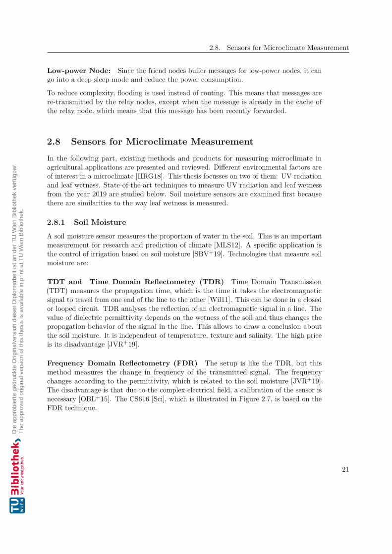
Frequency Domain Reflectometry (FDR) The setup is like the TDR, but thismethod measures the change in frequency of the transmitted signal. The frequencychanges according to the permittivity, which is related to the soil moisture [JVR+19].The disadvantage is that due to the complex electrical field, a calibration of the sensor isnecessary [OBL+15]. The CS616 [Sci], which is illustrated in Figure 2.7, is based on theFDR technique.
21

2. State of the Art
Figure 2.7: The CS616 [Sci] is a product from Campbell Scientific and is based on theFDR technique.
Figure 2.8: Resistor-based soil moisture sensor board from Sparkfun [Elea].
Soil Resistivity This method measures the resistance between two electrodes that areput in the soil. The moister the soil is, the lower the resistance is [CCC51]. The responsetime and the relatively high level of precision are advantages. Disadvantages are thenecessary calibration and the unstableness of it [FJ94]. Sparkfun sells a resistor-basedboard [Elea], shown in Figure 2.8.
Heidi Mittelbach et al. [MLS12] compare in her journal different soil moisture sensortypes and come to the conclusion that low-cost sensors, if they are calibrated, are a goodalternative to the expensive TDR sensors.
22

2.8. Sensors for Microclimate Measurement
(a) (b)
Figure 2.9: Schematic of resistor and capacitive measurement method. a) shows theschematic cut through the PCB for the resistor-based measurement and b) for thecapacitive-based measurement.
2.8.2 Leaf WetnessAn LWS emulates a leaf, by assuming that the wetness on the sensor is the same as onthe leaf. The correct emulation of a leaf depends on various factors, e.g. the color of thesensor [SMG04]. Ghobakhlou et al. compare [GAS15] different sensors and describe twomethods to measure the wetness on the emulated leaf. One method is to measure theelectrical resistance on a surface on which the Printed Circuit Board (PCB) tracks arenot protected by a solder mask as they have to be in direct contact with the water. Incase of the second method the PCB tracks are coated with a solder mask and the changein capacitance is measured. The solder mask is an additional protection for the sensorand it does not influence the measurement of the capacitance.
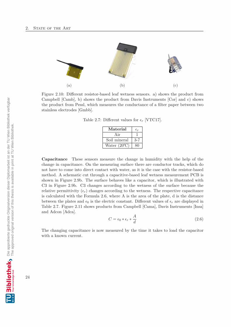
Leaf Resistivity The measuring surface consists of adjacent conductor tracks. Thesetracks are not protected by a solder mask because the water has to be in direct contact withthe copper from the tracks. If moisture hits this surface, the resistance changes becausea wet area conducts better than a dry one. A schematic cut through a resistor-based leafwetness measurement PCB is presented in Figure 2.9a. Products from Campbell [Camb],Davis Instruments [Cor] and Pessl Instruments [Gmbb] are shown in Figure 2.10.
23
2. State of the Art
(a) (b) (c)
Figure 2.10: Different resistor-based leaf wetness sensors. a) shows the product fromCampbell [Camb], b) shows the product from Davis Instruments [Cor] and c) showsthe product from Pessl, which measures the conductance of a filter paper between twostainless electrodes [Gmbb].
Table 2.7: Different values for r [VTC17].
Material r
Air 1Soil mineral 3-7Water (20℃) 80
Capacitance These sensors measure the change in humidity with the help of thechange in capacitance. On the measuring surface there are conductor tracks, which donot have to come into direct contact with water, as it is the case with the resistor-basedmethod. A schematic cut through a capacitive-based leaf wetness measurement PCB isshown in Figure 2.9b. The surface behaves like a capacitor, which is illustrated withC3 in Figure 2.9b. C3 changes according to the wetness of the surface because therelative permittivity ( r) changes according to the wetness. The respective capacitanceis calculated with the Formula 2.6, where A is the area of the plate, d is the distancebetween the plates and 0 is the electric constant. Different values of r are displayed inTable 2.7. Figure 2.11 shows products from Campbell [Cama], Davis Instruments [Insa]and Adcon [Adca].
C = 0 ∗ r ∗ A
d(2.6)
The changing capacitance is now measured by the time it takes to load the capacitorwith a known current.
24

2.8. Sensors for Microclimate Measurement
(a) (b) (c)
Figure 2.11: Different capacitive-based leaf wetness sensors. a) shows the product fromCampbell [Cama], b) shows the product from Davis Instruments [Insa] and c) shows theproduct from Adcon [Adca].
2.8.3 UV RadiationUV radiation is an electromagnetic radiation. It has too short a wavelength to be seen byhumans and is emitted by the sun. Artificial sources are Mercury-vapor lamps, Black lightlamps and UV- light emitting diodes [Dif02]. The electromagnetic spectrum of UV isdivided into three ranges, UVA, UVB and UVC; the corresponding wavelengths are shownin Table 1.1. UV is measured in watt per square meter. UV can be harmful to humans atcertain intensity [LGL+]. Therefore, the World Health Organization (WHO) introducedthe UV Index (UVI) for a better handling of the intensity. Plants use photosynthesis toconvert light energy into chemical energy [Ann92]. Therefore, UV radiation is importantfor plant growth, so the measurement is helpful for analyzing plant diseases [Hol02].
The following techniques are available to measure the UV value [Her13]:
Change in Temperature (Bolometer)
A Bolometer consists of a temperature-dependent electrical resistance, an absorptiveelement and a thermal reservoir. Radiation on the absorptive element causes a change intemperature, which can be measured with the help of the associated change in resistance.Bolometers have a response time of milliseconds [Dif13].
External Photoelectric Effect
The emission of electrons from the metal surface, when it is irradiated with radiation, iscalled external photoelectric effect. The Photomultiplier uses this effect and tubes tomeasure radiation [HP07].
25

2. State of the Art
Figure 2.12: Break out board for the VEML6075 by Sparkfun [Eleb].
Internal Photoelectric Effect
The internal photoelectric effect does not emit electrons like the external one. If the metalsurface is irradiated with radiation, it excites electrons to higher bands, namely from thevalence band to the conduction band. This results in a photo current on the p-n junctionor p-i-n junction. This effect is used in Photoresistors, Photodiodes, Phototransistorsand Charge-coupled Device (CCD)/Complementary metal-oxide-semiconductor (CMOS)detectors [Her13].
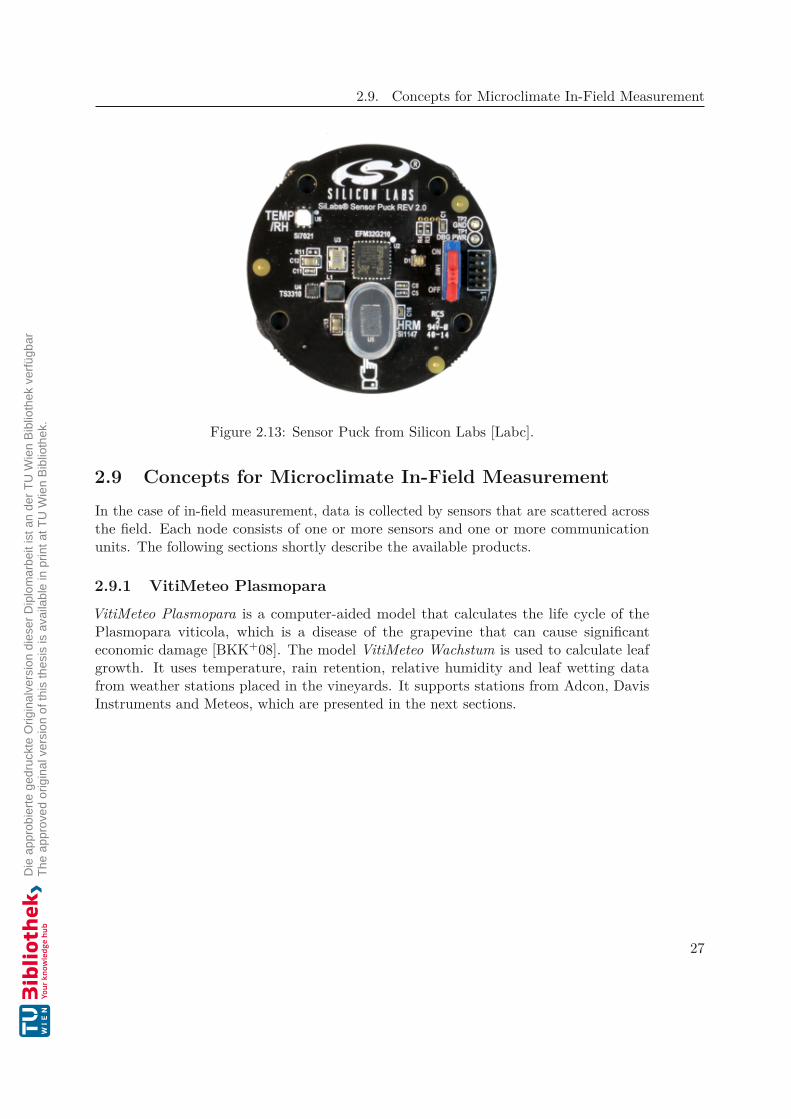
In IoT development, UV sensors can be bought on break out boards for evaluationpurposes. Two examples are the VEML6075 break out board from Sparkfun and theSensor-Puck from Silicon Labs. Sparkfun offers a break out board [Eleb] that containsall the necessary components for the VEML6075 to function correctly and also headerpins for connection. The board is displayed in Figure 2.12. The VEML6075 measuresUVA and UVB with photo diodes. The communication is managed by Inter-IntegratedCircuit (I2C), which is a two-wire serial data bus. Silicon Labs Sensor-Puck [Labc] is anenvironmental and biometric sensor board, which measures UV light with the Si1114xoptical sensor with the help of photo diodes. The Sensor-Puck is shown in Figure 2.13.It also includes a humidity and temperature sensor. The board can be supplied by a coincell battery. The EFM32 microcontroller is responsible for the collection and transmissionof measurement data via Bluetooth.
26
2.9. Concepts for Microclimate In-Field Measurement
Figure 2.13: Sensor Puck from Silicon Labs [Labc].
2.9 Concepts for Microclimate In-Field MeasurementIn the case of in-field measurement, data is collected by sensors that are scattered acrossthe field. Each node consists of one or more sensors and one or more communicationunits. The following sections shortly describe the available products.
2.9.1 VitiMeteo PlasmoparaVitiMeteo Plasmopara is a computer-aided model that calculates the life cycle of thePlasmopara viticola, which is a disease of the grapevine that can cause significanteconomic damage [BKK+08]. The model VitiMeteo Wachstum is used to calculate leafgrowth. It uses temperature, rain retention, relative humidity and leaf wetting datafrom weather stations placed in the vineyards. It supports stations from Adcon, DavisInstruments and Meteos, which are presented in the next sections.
27

2. State of the Art
Figure 2.14: Adcon Weather Station [Adcb]. a) is the main part called ADCON RTU.
2.9.2 AdconAdcon is a company with headquarters in Klosterneuburg, Austria. It offers sensors fortemperature, relative humidity, rain gauge, soil moisture, leaf wetness, wind directionand wind speed [Adcb]. The main part of the weather station is the ADCON RTUshown in Figure 2.14a). It is responsible for storing the data, the battery managementand for the transmission of data via radio. Supported radio technologies are GlobalSystem for Mobile Communications (GSM), General Packet Radio Service (GPRS),Universal Mobile Telecommunications System (UMTS). Data can also be transmittedvia Ultra-High-Frequency (UHF) signals. With the latest version, which is the series 6,Bluetooth can also be used to transmit data or to update the firmware.
2.9.3 MetosMetos is a company from Weiz, Austria. It offers sensors to measure leaf wetness,rain gauge, soil moisture and leaf temperature. Data is transmitted wirelessly viaLong Range Wide Area Network (LoRaWAN), GPRS, Enhanced Data Rates for GSMEvolution (Edge), UMTS or WiFi in a range of about 300 to 400 meters in a star topology.Data can also be transmitted over wire with Recommended Standard 232 (RS232). Themeasurements are stored on a cloud server. Figure 2.15 depicts the iMetos imt300, whichcontains sensors to measure temperature, humidity, rain gauge, soil moisture, leaf wetness,wind direction and wind speed.
28

2.9. Concepts for Microclimate In-Field Measurement
Figure 2.15: Metos Weather Station imt300 [Gmba].
2.9.4 DavisDavis is a California-based company that sells products for reliable weather monitoring.They offer weather stations for private, agriculture and safety-related measurements suchas windstorms and tsunamis. Their product portfolio contains all kinds of sensors forenvironment measurement. The EnviroMonitor [Insb] is a self-healing, reliable meshnetwork of environmental sensor nodes. Figure 2.16 shows an overview of the proposedsolution. The EnviroMonitor Gateway can collect data from up to 25 nodes. Dependingon the environmental conditions, the distance between nodes can be up to 1200 meters.Each node can connect up to 4 different sensors. The data is transmitted in the meshnetwork on a license-free band, e.g. in Europe 868.0 - 868.6MHz. The nodes are peeredwith the gateway and configured via Bluetooth. The gateway sends the data through thecellular network, e.g. Second generation mobile network (2G) or Third generation mobilenetwork (3G), to the Davis cloud server that is connected to the Internet. A standaloneweather station, which is additionally sold by Davis, e.g. the GroWeather (illustrated inFigure 2.16), can also be connected by a wire to the gateway. Nodes and gateways arepowered by a battery that is recharged with a solar panel. The gateway’s battery is a6V gel cell battery with 12Ah of capacity. It consumes about 25mA up to 1A. This way,the gateway can run for a minimum of 12h and a maximum of 20 days without charging.The node is powered by four D-cells or one lithium-ion battery (3,6V - 3,7V and about3000mAh) and typically consumes 12mA. This way, the node can run for 5 days withoutcharging. The company suggests using a 3W solar panel for charging. If the batteryvoltage is getting too low, the customer will be notified by email or a push message inthe mobile app.
29

2. State of the Art
Figure 2.16: Schematic structure of the EnviroMonitor mesh network [Insb].
Table 2.8: Costs of the Davis Instruments EnviroMonitor [Insb].
Type one-off costs[$] annual costs for 15-minute interval[$]
Gateway 795 220Node 395 30Sum 1180 250
In the manual the producer claims a runtime of multiple years under optimal conditions.Problems could arise if the solar panel is shaded (by vegetation, snow or dirt) or if it isturned away from the sun. The price of an EnviroMonitor Node is $395 and that of thegateway is $795. For an update interval of 15 minutes, the yearly cost for the gateway is$220 and for one node it is $30. This means that the customer gets new data every 15minutes; the storage is supplied by Davis Instruments. In Table 2.8 the overall costs forone year with prices as per October 2019 are listed.
2.9.5 Libelium
Libelium is a Spanish company that offers different solutions for IoT. It has two mainproduct lines. One is based on a development board called Waspmote, which is a hardwareboard with various built-in features for IoT devices. The second line is the WaspmotePlug & Sense, which is a commercial product containing the Waspmote board withdifferent sensors connected to it.
30

2.9. Concepts for Microclimate In-Field Measurement
(a) (b) (c)
Figure 2.17: Waspmote and Waspmote Addons [Lib]. a) shows the hardware boardWaspmote, b) shows the Waspmote 802.15.4 radio board, and c) shows the WaspmoteAgriculture Sensor board, with different sensors.
Waspmote The hardware board shown in Figure 2.17a contains an ATmega1281 mi-crocontroller and interfaces to connect different sensors and radio boards. The supportedradio technologies are 802.15.4 (radio board shown in Figure 2.17b), LoRaWAN, WiFi,Fourth generation mobile network (4G) and Bluetooth. The company offers open-sourceSoftware Development Kits (SDKs) and Application-Programming-Interfaces (APIs).They support peer-to-peer, star and mesh topologies. For the mesh topology, DigiMesh[Inca] with its own radio board is used. Sensor boards are available for different use cases,e.g. for agriculture measurements, gas measurement, flood protection and smart parking[Lib]. The Waspmote consumes 17mA while active, whereas the power consumptiondecreases to 7µA in hibernate mode. Supported battery voltages range from 3.3V to4.2V. The battery is charged with a solar panel or Universal Serial Bus (USB). TheWaspmote hardware board with the 802.15.4 radio board costs about e240 and a sensorabout e75.
31

2. State of the Art
(a) (b)
Figure 2.18: Ready-to-use products from Libelium [Lib]. a) shows the Waspmote Plug &Sense and b) shows the Meshlium 4.0.
Waspmote Plug & Sense The Waspmote Plug & Sense is a ready-to-use productand comes with an IP65 waterproof enclosure, which is depicted in Figure 2.18a. Externaldevices, such as sensor probes, batteries, solar panels or USBs can be plugged in easily.Inside, the Waspmote and the radio board are installed, depending on the technologyused.
Meshlium The Meshlium, presented in Figure 2.18b, is a gateway from the sensornetwork to the Internet. It receives data from the sensor nodes over different radiotechnologies and sends it over a cellular connection to a cloud server connected to theInternet. Specification:
• CPU: 1GHz
• RAM: 2GB
• SSD: 16GB
• OS: Linux, based on kernel 3.16
• Consumption: 15W, but it heavily depends on the number of activated radios
2.10 Microclimate Measurement With SatellitesEarth Observation Satellites (EOS) are obtaining information about the earth’s surface.They operate in an altitude of about 36000km. The satellite data can be used to assessthe canopy surface (e.g. detect the presence of weeds) or the canopy structure (e.g.measure crop height), and it can also help in decision making (by e.g. predicting yields)[ahd19]. Mark Jarman describes in his reviews [ahd19] available satellite technologies foragricultural applications. He also gives an overview of the usability of some products.
32

2.10. Microclimate Measurement With Satellites
Two companies offering analysis of satellite or drone images to farmers are Descartes-Labs and FarmShots. DescartesLabs [Labb] offers the recognition of valuable data fromsatellite images. Their methodology is to construct models of real-world processes thatare fed with relevant input (e.g. satellite imagery). FarmShots [Sho] offers the analysisof satellite and drone images.
33


CHAPTER 3Requirements and Design
Decision
This chapter focuses on the hardware and software requirements that are necessaryto build a sensor network for agricultural microclimate measurement. Based on thesespecifications and the state of the art, which was looked at in the previous chapter, wewill decide on the design later on.
3.1 Hardware RequirementsIn this section the hardware requirements for the sensor nodes are defined. These devicesare installed outdoors to measure the microclimate and should be as flexible as possible.In order to achieve this, the following features must be considered:
• Outdoor Usage Since the aim is to measure the agricultural microclimate, thesensor nodes have to be placed in the fields, vineyards or orchard. Therefore, theyhave to be constructed to be able to tackle different environmental conditions (e.g.heat, cold, humidity) without suffering damages.
• Size The nodes should fit into trees and walls of grapevine leaves. The leaf wetnesssensor area should imitate the size of a half-grown leaf. We took the leaf ofthe Grüner Veltliner as a reference, which is about 7x7cm in size [Bau08]. Theremaining part of the sensor must not exceed 10x10cm, otherwise it could influencethe foliage growth.
• Easy Installation Since a swarm consist of many sensors, the mounting and setupshould be easy and fast. Due to necessary mechanical work steps, such as vinecutting, it may be necessary to demount some sensors annually. The process shouldnot take more than 10 minutes for a sensor.
35

3. Requirements and Design Decision
• Extension After the initial configuration of the network, it should also be possibleto add new sensor nodes.
• Self-Sufficiency The sensor nodes should be energetically self-sufficient. Thismeans that the sensors generate the energy they require by themselves as best aspossible.
• Price The currently available products, which were already presented in Chapter2, are in no case available for less than e1100 per node. In order to enable smallerfarms to buy a sensor network, we tried to keep the price below that of the alreadyexisting products. This means that the price of ten sensors and one relay nodeshould not exceed e1100.
• Different Power Sources It should be possible to supply the device with differentpower sources, e.g. USB, Solar, Battery, power supply.
• Battery Power For the periods of time where no sunlight is available, the batterymay provide the energy for the sensor. We assume that no sunlight is availablefor at least 12 hours on any given day. This means that the battery must be ableto supply power for at least 12 hours. The aim is to provide more capacity thanneeded. The gateway itself can be connected to the power grid and therefore doesnot need a battery.
• Solar It is one of the available power sources to load the battery and power thesystem. The solar panel should minimize the need to change batteries. The size ofthe solar panel should be dimensioned so that it can fully charge the battery duringone day. Attention should also be paid to the solar radiation of the test region thatis located in Austria, in the state of Lower Austria, in the region called "Kremstal".
• Wireless Connectivity It should be used to transmit the data to the gatewayand further to the Internet, without the need of installing wires. This way, theadaption and setup of a wireless sensor network takes less time than in the case ofa wired one. The sensors should therefore use a wireless connection, on the otherhand the gateway can be connected with a cable to the Internet. The disadvantagesare the higher power consumption of wireless sending and the susceptibility tointerferences [YKX+17].
36

3.2. Software Requirements
3.2 Software RequirementsIn this section the software requirements for the sensor nodes are defined.
• Mesh Network In order to transmit the measurement data to a cloud serverconnected to the Internet via a gateway, a reliable and self-healing network isnecessary. As discussed in 2.1 a mesh network is the best choice for this purpose.
• State Of Charge (SOC) The battery voltage should be monitored for optimizingthe energy consumption and for sending an alert if the battery is low.
• Extension It has to be possible to add new sensor nodes to the network.
3.3 Measurement RequirementsIn this section we specify the requirements for the values to be measured. The followingmain criteria must be taken into account:
• UV It is essential for photosynthesis and UV measurement also helps in the analysisof plant diseases [Hol02]. UVC is blocked by the ozone layer and is not importantfor our measurement [SSS+06]. The sensor should thus measure UVA and UVB.
• Leaf Wetness The Leaf Wetness Duration (LWD) is an important variable fordisease-development and disease-warning systems [Mon13]. Therefore, the leafwetness should be measured.
• Vicinity The sensor should be installed near the target objects, otherwise themeasurement results could be falsified. For example, if a leaf casts a shadow over asensor, the leaf is in a different "environmental state" than the sensor that shouldimitate it.
• Synchronization It is important that the sensors record measured values at aboutthe same time, to enable a comparison of the data. The reference to the globaltime is then established via the node, which has an Internet connection.
• Frequency The interval for taking a measurement should be adjustable accordingto the type of value that should be processed, the location (e.g. vineyard or orchard)and the available storage space in the sensor.
3.4 ComparisonIn the following section we compare the existing solutions, which were presented inChapter 2. All the products are suitable for outdoor usage, have wireless connectivityand optimized power consumption, are battery-powered and extensible with new sensors.All the nodes can be programmed Over The Air (OTA).
37

3.R
equirements
andD
esignD
ecision
Table 3.1: Comparison of existing solutions.
Properties Waspmote WaspmotePlug&Sense
Adcon Metos Davis
Leaf Wetness Sen-sorUV Sensor UVA and UVB UVA and UVB UVA UVA and UVB UVAMesh capabilities × ×Size without sen-sors
73.5 x 51 mm 85 x 122 mm 160 x 60 mm 410 x 130 mm 210 x 280 mm
Price gateway [e] 1500 1500 not needed not needed about 795Price node [e] 240 1025 1700 about 3000 about 395Var. price node [e] 75 per sensor 34 per sensor 4G, 10GB about
10 monthly4G, 10GB about10 monthly
250 monthly forone node
Supported proto-cols
802.15.4, Lo-RaWAN, WiFi,4G, BLE
802.15.4, Lo-RaWAN, WiFi,4G, BLE
2G/3G or 4G/LTE GSM, GPRS,EDGE, HSDPA,CDMA, UMTS,Satellit, WiFi,LoRa
GSM, UMTS
Open Source not all not all × × ×
38

3.5. Design Decision
3.5 Design DecisionAdcon and Metos are not able to build a mesh network, they only support mobile cellularnetworks. Therefore, each node comes with monthly costs for a Subscriber IdentityModule (SIM) card to get a cellular connection. Since the aim is to place more than 10sensors in one field, this is not an economical solution. Furthermore, the costs of theAdcon and Metos sensors exceed the previously defined budget.Davis Instruments supports mesh networks with their own closed software on a license-freeband. The price for the gateway is high (about e795), but we would need only one, so itis affordable. But the high costs of buying one node and the additional monthly costs forevery node to store the data on their servers exceed the previously defined budget.The Waspmote Plug&Sense would be the best solution for our needs, but the costs alsoexceed the previously defined budget. The Waspmote would be a good starting pointto develop further sensors. Unfortunately, it has a lot of extensions that we don’t needbut cannot be deselected at purchase either. So this option also exceeds our previouslydefined budget.Based on the literature survey and the analysis of existing solutions, we decide to developour own board. It will only contain the mesh functionality and we will be able to use itas a model for further sensors in IoT applications. In the next chapter we compare andselect the components for the sensors and also choose a transmission technique.
39


CHAPTER 4System Design
In this chapter we list and compare possible solutions and products - that we build fromself-developed hardware and software - that can fulfill the specific requirements. Afterthis, we select the appropriate components based on the requirements, product researchand the literature survey.
4.1 LWSAn LWS measures the moisture on a leaf by imitating it. The requirements for the LWSare robustness, reliability and longevity. Therefore, we choose the capacitive measurementmethod, which was discussed earlier in Section 2.8.2. The goal is to develop a board withhigh sensitivity to measure leaf wetness. To do this, three boards with different PCBlayouts should be designed; Figure 4.1 provides an illustration. We will compare theboards in Chapter 7. Each of these boards changes its capacity relative to the moistureon the surface to be measured. We are not interested in measuring the exact capacity inFarad, but in getting a value related to the wetness, e.g. 0 indicates not wet and 100means wet. Three ways to measure the change in capacity are:
Difference Method A capacitor is unloaded and the voltage is measured at twodifferent known time points [Dja19]. With Equation 4.1 we can calculate the value ofthe capacitance. In Figure 4.2a the circuit and in Figure 4.2b the discharge curve isillustrated. This method is mainly used in multimeters.
C = t2 − t1
R ∗ ln(U1U2
)(4.1)
41

4. System Design
(a) (b) (c)
Figure 4.1: Different conductor thicknesses to test the moisture sensitivity. a) shows thewetness area with large tracks, b) shows the wetness area with medium tracks and c)shows the wetness area with small tracks.
R C
V
(a) Discharge circuit.
U
(0,0) t
U1
t1
U2
t2
(b) Discharge curve.
Figure 4.2: Capacitance measurement with the difference method.
Capacitive to Digital Converter A Capacitive to Digital Converter (CDC) is anIntegrated Circuit (IC) that measures the capacitance and is mainly used in touch-screens,humidity sensing or liquid level sensing devices and pressure measurement [Nin12]. Forexample, the AD7746 [Dev], schematically shown in Figure 4.3, measures the capacitancewith switching capacitor technology. It contains a known and fixed excitation voltage,reference voltage and an internal reference capacitance. The converted value from theSigma-Delta modulator represents the ratio between the sensed capacitance and thereference capacitance. Different CDCs are compared in Table 4.1.
42

4.1. LWS
Figure 4.3: CDC Simplified Block Diagram of the Analog Devices AD7746 [Dev].
Table 4.1: Comparison of CDC.
Price [e](09/2019)
Size [mm] Accuracy[fF]
Range [pF] Supply Volt-age [V]
AD7746 12 5 x 6 4 ±4 2.7 - 5.25FDC1004 5 3 x 3 0.5 ±15 3.3LC717A00AJ 1.96 8 x 6.4 0.04 ±8 2.6 - 5.5
Capacitance Measurement Using Low Pass Filter With the help of a low passfilter, the change in capacitance can be measured [RSPAM19]. A low pass filter passessignals with frequencies lower than the cutoff frequency (e.g. f13db in Figure 4.4) andweakens signals with higher frequencies. This is illustrated in the Bode diagram 4.4. Thecutoff frequency can be calculated with Equation 4.3. A circuit for a first order low passfilter consists of a resistor and a capacitor. This is illustrated in Figure 4.5.
G = 20 log Uout
Uin(4.2)
f3dB = 12πRC
(4.3)
From Equation 4.3 we can see that if the capacitance C changes, the cutoff frequencychanges. If we feed our input Uin with a rectangular signal with a fixed frequency fin
(e.g. 1MHz), the output voltage is weakened according to the capacitance. This behavioris illustrated in Figure 4.6, in the time domain for a 1nF (C1) and a 3nF (C2) capacity.These values were taken based on a measurement from a capacitance sensor in wet(C2) and dry (C1) states. The resistor was set to 330Ω. The input voltage was set to3.2V because this will be the supply voltage. The voltage curve over the time whenthe capacitor is charging can be calculated with Equation 4.4, the discharging can becalculated with Equation 4.5.
43

4. System Design
102 103 104 105 106 107 108
−60
−40
−20
0
f13db
f23db
fin
f [Hz]
G[d
B]
Bode diagram
Figure 4.4: Bode diagram of a first order low pass filter. The green line with cutofffrequency (f13db) shows the damping of the input signal with a big capacitance and theblue line (f23db) for a smaller one. The frequency of the input signal is 1MHz ( fin).
R
CUin Uout
Figure 4.5: Low pass filter circuit.
Figure 4.4 shows the Bode diagram of this behavior, where fin is fixed at 1MHz. Thegreen line illustrates the damping of the input signal with a big capacitance and the blueline for a smaller one. For the high capacitance (wet area) and for the small capacitance(dry area), the input signal is damped by -20dB per decade.
uc(t) = U0 ∗ (1 − e−t
R∗C ) (4.4)
uc(t) = U0 ∗ e−t
R∗C (4.5)
We are choosing the capacitance measurement using a low pass filter because the compo-nent, consisting of a resistor and a capacitor, cost €0.2 at Mouser in 2019 and this priceis lower than that of a CDC.
44

4.2. UV Sensor
0 0.2 0.4 0.6 0.8 1
0
1
2
3
t [µs]
U(t
)[V
]
UC1UC2Uin
Figure 4.6: Capacitor charging and discharging curves in steady state. C1=1nF (dryleaf) and C2=3nF (wet leaf)
Table 4.2: Comparison of UV sensor ICs
Product Price [e](09/2019)
Size [mm] Range [nm] I2C Supply Volt-age [V]
Si1133 1.48 2 x 2 280-400(only UV-Index)
1.62 - 3.6
VEML6070 2.36 2.35 x 1.8 320-400 1.7 - 5.5VEML6075 2.7 (End of
life)8 x 6.4 280-400 1.7 - 3.6
AS7341 8.24 3.1 x 2 350 - 1000 1.8
4.2 UV Sensor
The UV sensor should measure UVA (320-400nm) and UVB (280-320nm). In Table 4.2different UV Sensors are compared. Unfortunately, the Si1133 does not directly measureUV, it only performs UV Index approximation based on the light level. The VEML6070and VEML6075 have a light sensor to measure the UV spectrum. The VEML6075would be the best choice because it measures UVA and UVB, but it is an end-of-lifeproduct. The VEML6070 measures only UVA. The AS7341 does not measure the fullUVA spectrum. So we are choosing the VEML6070.
45

4. System Design
Table 4.3: Comparison of Bluetooth Mesh and Thread Mesh network [MLPP16].
Properties Bluetooth Mesh ThreadRouting techniques Flooding Routing and floodingAmount of connectednodes
Low High
Range Low Low6LoWPAN support
4.3 Data TransmissionIn the following section we examine different possibilities to transmit data from the sensornodes to the cloud. These data transmission opportunities can be implemented withoutchanging the hardware, only the software needs to be adapted accordingly. Figure 4.7depicts the schematic design of the transmission network and its layers. In the firstregion, the sensor nodes are connected with a mesh network, this is called the sensorswarm. Based on Table 4.3, we choose Thread as protocol for the mesh network becauseof the lower power consumption of the routing technique [MRC+17], which is one of ourdiscussed requirements in Section 3.1. Each node forwards received messages that donot belong to themselves to all other reachable nodes with the flooding technique. Therouting technology determines the routes of the messages in advance. This is done withthe help of routing tables. In the fog layer, data is collected from the mesh network oversome gateway and is then forwarded to the cloud. The fog layer contains devices that cancommunicate with the mesh network and have an Internet connection, e.g. a smartphone,a quadrocopter or a Raspberry Pi. Since smartphones [SWA13] and the Raspberry Pi[Upt19] have Bluetooth built in, this is used to communicate with devices in the meshnetwork. The sensors that operate as a gateway and that are called relay nodes need toimplement Thread and Bluetooth. The Internet connection can be established via cableor the cellular network. Nodes in the fog layer have higher computation power and morestorage. Therefore, they can set actions based on the data. In the cloud region the datais stored on a cloud server connected to the Internet.
Figure 4.8 illustrates different transmission possibilities. They will be implemented inChapter 6 and compared in Chapter 7.
46

4.3. Data Transmission
Figure 4.7: Schematic design of the sensor network.
47

4. System Design
• In variant 4.8a, called Forward Only Method, messages are sent periodically by eachsensor. The relay node forwards these messages immediately to a connected fognode. If no fog node is available, the message is lost. On the one hand this is thedisadvantage of this variant, on the other hand an advantage is that no buffer isneeded.
• In variant 4.8b, called Relay Buffered Method, messages are sent periodically byeach sensor. The relay node buffers the data until a data request from the fog nodearrives. After that, it forwards all buffered data to the fog node and clears thebuffer. Response technique is used as communication protocol. The disadvantage isthat the buffer of the relay node is related to the number of sensors in the network.Therefore, the number of sensors in the network cannot be increased withoutconsidering the remaining free buffer space of the relay node. The advantage isthat the fog node does not have to be connected to the network all the time.
• In variant 4.8c, called Fog Request Method, each sensor buffers the measured datauntil a data request from the relay node arrives. After that, each notified sensorsends its data to the relay, which then forwards it to the fog node. Responsetechnique is used as communication protocol. The disadvantage is that each sensorneeds a buffer to store the sensor values and a time synchronization. The advantageis that if a sensor loses the connection to the network, the measurement values donot get lost because they are stored locally.
The Relay Buffered Method and the Fog Request Method are based on the request andresponse technique, which is not supported by MQTT (see Table 2.5). Therefore, CoAPis used as communication protocol.
48

4.3. Data Transmission
(a)
(b)
(c)
Figure 4.8: Different transmission possibilities. a) shows the Forward Only Method, b)shows the Relay Buffered Method and c) shows the Fog Request Method. The semicolon-separated list illustrates the following data: "ID of the sensor; Type of Measurement;Value; Time"
49

4. System Design
Table 4.4: Comparison of data storage consumption. The abbreviation for the pick-upinterval is PUI, MI stands for measurement interval, NS means number of sensors andSD stands for size of data. PUI and MI are measured in seconds and SD in bytes.
Variants Sensor Swarm [Byte] Relay node [Byte]
Forward Only Method 0 0
Relay Buffered Method 0 P UIMI ∗ SD ∗ NS
Fog Request Method P UIMI ∗ SD 0
4.3.1 Data StorageSince the available storage on the sensor nodes is limited, we have to calculate the needsand optimize the data collection in that way. We assume that the fog node (e.g. aRaspberry Pi) has unlimited storage. In the Forward Only Method, 4.8a, the sensorand relay node only need a buffer to store the measurement temporarily until it istransmitted to the fog node. In the Relay Buffered Method, 4.8b, the sensor needs abuffer to temporarily store the measurements until they are transmitted to the relaynode. The relay needs a buffer to store the measurement values from all sensors until thefog node collects it. In the Fog Request Method, 4.8c, each sensor stores the data untilit is collected from the relay node. The relay only needs a buffer to temporarily storethe measurement values until they are transmitted to the fog node. Table 4.4 presentsa comparison of these methods. The abbreviation for the pick-up interval is PUI, MIstands for measurement interval, NS means number of sensors and SD stands for sizeof data. PUI and MI are measured in seconds and SD in bytes. The leaf wetness cantake values between 0 and 100 units. Therefore, it is stored in a variable with a sizeof one byte, which can have a maximum value of 255. The UV value, according to thedata sheet of the VEML6070 [Sem19], has the size of two bytes. Two bytes are requiredto store the time of the measurement. This way, it is possible to store 45 days with aminute resolution and 18 hours with a second resolution. These two bytes are needed forthe leaf wetness and the UV measurement values if they have different recording times.In total, 5 bytes of memory are required for the data, which corresponds to the variableSD. Table 4.5 displays the results when we collect the data every week, set the numberof sensors to ten and the measurement interval to one minute.
50

4.4. System on Chip
Table 4.5: Comparison of data storage. Data storage (SD) is set to 5 bytes. The pick-upinterval (PUI) is set to one week. The measurement interval (MI) is set to one minuteand the number of sensors (NS) is set to ten.
Variants Sensor Swarm [Byte] Relay node [Byte]
Forward Only Method 0 0
Relay Buffered Method 0 7∗24∗60∗6060 ∗ 5 ∗ 10 = 504k
Fog Request Method 7∗24∗60∗6060 ∗ 5 = 50.4k 0
4.4 System on ChipA SoC is a chip that contains different ICs for different functionalities. A SoC can containa processor, a voltage regulator and different interfaces and components for storage (Flashor Random Access Memory (RAM)). The SoC is the main part of the sensor board andhas to fulfill the following requirements:
• Support BLE and 802.15.4 The hardware needs to support BLE and 802.15.4,this is necessary for the wireless transmission of the data.
• Serial Peripheral Interface (SPI) and I2C Necessary for the on-board com-munication with other ICs.
• Analog to Digital Converter (ADC) Necessary for converting the analogcapacitive leaf wetness value to a digital value.
• Minimum Flash As calculated in Table 4.5, the minimum free flash storage on arelay node has to be 504kB and on a sensor node 50.4kB.
• Bluetooth Stack A Bluetooth stack is software that implements the Bluetoothprotocol. If a Bluetooth stack is already provided by the SoC producer, thedevelopment of the transmission software takes less time because the Bluetoothstack does not have to be implemented.
• Thread Stack A Thread stack is software that implements the Thread protocol.If a Thread stack is already provided by the SoC producer, the development of thetransmission software takes less time because the Thread stack does not have to beimplemented.
51

4. System Design
Table 4.6: Comparison of SoCs.
Producer Silicon Labs Nordic Semi-conductor
Texas Instru-ments
ON Semicon-ductor
Part number EFR32MG12 nRF52840 CC1352P NCS36510MCU Core ARM Cortex
M4ARM CortexM4F
ARM CortexM4F
ARM CortexM3
Frequency[MHz]
40 64 48 32
Flash [kB] 1024 1024 256 640RAM [kB] 256 256 80 48ThreadBLE ×GPIO Pins 65 48 18 26Package Type BGA125 AQFN-72 VQFN48 QFN-40Energy con-sumption TX[mA] at 0dBm
8.5 4.8 7 7
Price (Mouser10/2019) [e]
10.36 5.45 9.32 5.63
Table 4.6 compares SoCs from Silicon Labs, Nordic Semiconductors, ON Semiconductorsand Texas Instruments. They all have I2C, SPI, Pulse Width Modulation (PWM) andan ADC. Based on Table 4.6 and the requirements, the nRF52840 is the best choicefor our project. The NCS36510 does not support Bluetooth and BLE and therefore itdoes not fulfill the transmission requirements for a relay node. The EFR32MG12 andthe CC1352P would also work well. However, the nRF52840 has a greater flash and alower price. So we decide to use the nRF52840.
4.5 Power ManagementThe power management is responsible that the system has always enough energy. Toensure this, a solar panel and a battery are installed on the device. Furthermore, USBcan be used as an optional third source. If USB is connected, this is the preferred choicefor the power source as it provides reliable power. Unlike the solar panel, which dependson sunlight. If a power source is connected, disconnected or exceeds the configuredmaximum or minimum voltage, a seamless switch to another power source should takeplace. Before comparing possible components for the power management, facts for laterdecision making are presented.
52

4.5. Power Management
Thermistor Thermistor is used to measures the temperature based on the resistancechange. It is needed to monitor the temperature of the battery during charging becausecold and hot batteries should not be charged fast [Ins18].
Voltage Proportional Current Control (VPCC)/Voltage Input Dynamic PowerManagement (VINDPM) It is a feature that regulates the consumed current bythe voltage. If, for example, a battery charger consumes too much current from asource, the voltage drops and the consumed current is reduced. The voltage threshold iscomponent-dependent and is either set to a fixed value or can be configured with I2C ora voltage divider.
Dynamic Power Path Management (DPPM) Manages and controls the flow ofthe current based on the voltage. If the input voltage drops under a defined threshold,the charging of the battery is throttled; if the voltage drops further, the charging isstopped and the battery is used to power the system. This is all done seamlessly so thatthe output is powered continuously.
Dynamic Power Management (DPM) Regulates the input voltage or the inputcurrent against a threshold by modifying the current consumption. It is more efficientthan using DPPM and the system voltage is always constant. But a voltage drop calledbrownout could crash the system.
Maximum Power Point Tracking (MPPT) Describes the way to get the maximumpower out of a solar cell. It is illustrated by a black line in Figure 4.11. The maximumpower from a source is obtained when the product of current and voltage is at itsmaximum. This is the case when the internal resistance of the source is equal to theload resistance. This operating point is commonly called Maximum Power Point (MPP)[PRSBR17].
Power Multiplexer Switches between input sources. The switch should be seamlessso that the system is continuously powered all the time. Our aim is to make sure thatthe power Multiplexer (mux) switches to the most reliable input source and preventsdamage through timely switching in the event of voltage peaks.
4.5.1 Circuits for Power ManagementIn the following sections, three possible power management designs are examined. Thecircuit that suits our needs best is then selected.
53

4. System Design
Figure 4.9: Schematic of the BQ2403x dual input charger IC from Texas Instruments[Ins14].
Figure 4.10: Schematic of the power mux TPS2121 connected to the battery chargerBQ25895. Both components are from Texas Instruments.
Variant 1: Dual Input Charger IC
A dual input charger IC manages two inputs to load the battery and to power the systemat the output pin. It uses Power Path Management (PPM) and predefined thresholds tochoose one of two inputs. The schematic of the BQ2403x, which is a dual input chargerIC from Texas Instruments, is shown in Figure 4.9. Table 4.7 compares the componentsavailable on the market. None of these ICs have dual input or MPPT. But they all haveDPPM.
Variant 2: Power Mux With a Single Input Charger IC
In this design a power mux switches one of two inputs to the battery charger IC. Figure4.10 shows the schematic. The battery charger IC needs only one input. Table 4.7 listsavailable products on the market. They all have DPPM and a Negative TemperatureCoefficient (NTC). Table 4.8 lists different power muxes.
54

4.5. Power Management
Table 4.7: Comparison of single and dual input charger ICs.
Products ComponentsPrice [e] Size [mm] VPCC[V]
MPPT Inputs
BQ25895 8 2.85 4.8 x 4.8 3.9 - 15.3 × 1FAN54063 8 2.5 2 x 2 3.5 - 4.5 × 1LTC4162 15 8,57 4 x 5 4.2 - 4.6 1MAX77818 11 5.08 3.6 x 3.6 4.3 - 4.5 × 1BQ24032 8 3.66 3.5 x 4.5 2.6 - 5 × 2BQ24161 10 3.7 2.8 x 2.8 4.2 - 4.7 × 2LTC4155 9 6 4 x 5 4.3 × 2FAN54511 9 4 4 x 5 - × 2
Table 4.8: Comparison of power muxes available on the market.
Products Components Price [e] Size [mm] OperationRange [V]
TPS2121 6 1.81 1.5 x 1.9 2.8 - 22FPF3042 5 1 1.96 x 1.76 4 - 12.4LTC4412 5 1.4 1.5 x 2.9 2.5 - 28
Variant 3: Single Input Charger IC
Here we only need the battery charger, the switching between battery and the inputvalue is performed by a Metal Oxide Semiconductor Field Effect Transistor (MOSFET).The cable from the solar panel is connected with a Direct Current (DC) jack to the board.If a solar panel is plugged into the DC jack, the second input source is mechanicallydisconnected by it. As soon as an input voltage is applied, the system is supplied withits power and the battery is charged. We can use the MCP73871 or one of the previouslydescribed single input charger ICs as battery charger.
55

4. System Design
4.5.2 Design DecisionThe problem with the dual input variant is that no product supports a solar cell very well.Figure 4.11 illustrates the origin of this problem. If we follow the orange line (markedwith 1) from the right, we see that at 0.5V the current rises. At roughly 0.45V we havethe MPP with 36mA and at about 0.4V the maximum current, which is 38mA, is reached.As soon as more than 38mA of current is drawn, the orange line for the voltage goestowards 0V. If a battery charger does not consider this voltage drop, it will abort theloading and continue it at a later time. This results in a non-stop charge and is thereforeless efficient than charging continuously at constant current. Therefore, we need a VPCCto regulate the current consumption. The blue line in Figure 4.11 shows the MPPT.
The curves in Figure 4.11 are for one diode, where the consumption is 0.5V, due to thep-n junction. To get a higher voltage, the diodes can be put in series. The different linesindicate how strong the illumination of the sun is. For example, the orange line (markedwith 1) at 38mA has the most illumination.
The BQ24032 has VPCC, but the voltage is limited to 5V, which is too low because asolar cell could have its MPPT at higher voltages, depending on the solar cells connectedin series.
The power mux and the single input charger IC variant do not have to deal with thisproblem because both use the single input charger ICs for loading, which supports VPCCwith higher voltages. The advantages of the variant with the power mux over the singleinput charger IC are low component costs, the over-voltage protection and the automaticswitch to another input. Therefore, we will choose this variant. We use the BQ25895 asa charger IC because of its high VPCC voltage. The LTC4162, which has MPPT, wouldalso meet our requirements, but is three times more expensive than the BQ25895.
To compensate for the lost efficiency due to not using MPPT, we use a larger solar panel.Since solar panels are available only in standard sizes, we can not order one which fitsexactly our calculation. Therefore, we take the next bigger standardized panel.
4.5.3 Approximate Power ConsumptionIn this section, the power consumption is calculated as an approximate value. This valueis needed to roughly calculate the size of the battery and the solar panel. First, we takethe current consumption of the nRF52840. The values in Table 4.9 were obtained fromthe data sheet. The ADC is used to convert the measured analog leaf wetness value toa digital value. The watchdog monitors the digital system to detect malfunctions. If afailure is detected, the watchdog can reset the system. The radio has to be in receivingmode the whole time, otherwise the mesh network loses its function and messages canget lost. Sleepy end devices could turn off the radio and therefore need less current, butwe are dimensioning the devices for the worst case, which is when the radio is poweredall the time.
56

4.5. Power Management
Figure 4.11: Solar Cell IV curve with MPP [Com06].
Table 4.9: Current consumption of nRF52840 [Sem16].
Radio receiving 6.53mAADC active 1.24mA
Watchdog active 3.1µA
Sum 7.77 mA
The current consumption of the BQ25895, if the battery is discharging, i.e. there is novoltage on VBUS, is 12µA. If the battery is charging, the BQ25895 consumes 3mA. TheTPS2121 consumes 300µA if one of the two inputs power the output. If none of theinputs are connected, the TPS2121 is on standby and consumes 15µA. For the overallconsumption in battery mode, we add the values as shown in Table 4.10. We get anoverall current consumption of 7.9mA, which tells us that we can operate our sensorfor about 5 days, with a 1,1Ah battery. This fits our requirement, which we defined inSection 3.
57

4. System Design
Table 4.10: Overall current consumption, in battery mode.
NRF52840 7.77mABQ25895 12µATPS2121 15µA
VEML6070 100µA
Sum 7.9mA
Table 4.11: Comparison of rechargeable batteries [Mor12].
Type SpecificEnergy[Wh/kg]
RechargeCycles
Life [years] Self-DischargeRate permonth
Price perWh [e](09/2019)
Lead-Acid 35-50 250-1000 5 up to 20% 0.19Nickel-Iron 50-60 2000 20 up to 40% 0.9Nickel-Cadmium
30-60 1000 to 50k 10-15 up to 15 % 2
Nickel-Metal-Hydride
60-80 300-600 2-5 up to 25% 1.25
Lithium-Ion
80-180 3000 5+ up to 10% 0.9
4.5.4 BatteriesBatteries convert chemical energy to electrical energy. The battery for the sensor boardshould store the produced surplus of the solar panel for times when solar energy cannotbe used. Therefore, it should be rechargeable, have a high lifetime, low self-discharge,low price per Watt hour (Wh) and low weight. The rounded-up power consumptionfrom Table 4.10 is 8mA. For 24 hours a minimum battery capacity of 192mAh is needed.Morris [Mor12] compares the different batteries. All batteries relevant for the sensordevice are summarized in Table 4.11. We defined in Chapter 3 a portable and smallsensor, so we need a light-weight battery. The Lithium-Ion is the best choice. It is cheapand has the lowest self-discharge rate. The battery has to be charged only once a day, sothe maximum number of recharge cycles will be reached in about 8 years. A rechargecycle indicates how many times the battery can be fully charged and discharged [Dav10].
58
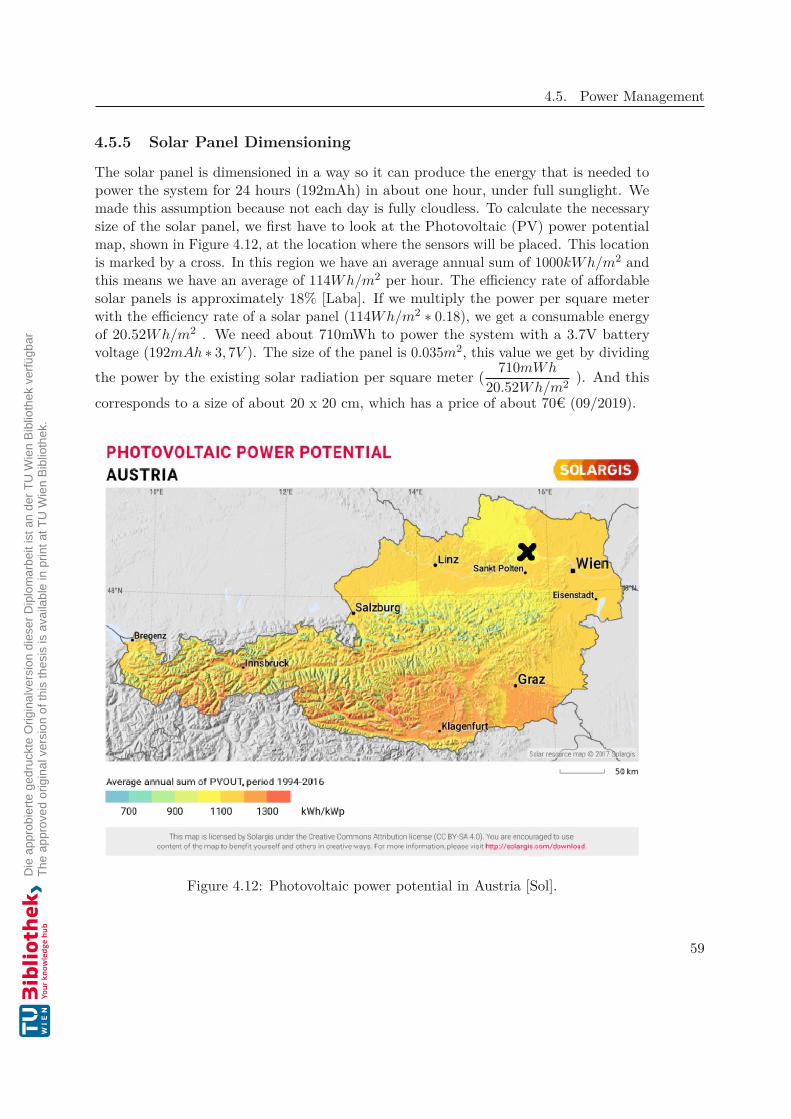
4.5. Power Management
4.5.5 Solar Panel Dimensioning
The solar panel is dimensioned in a way so it can produce the energy that is needed topower the system for 24 hours (192mAh) in about one hour, under full sunglight. Wemade this assumption because not each day is fully cloudless. To calculate the necessarysize of the solar panel, we first have to look at the Photovoltaic (PV) power potentialmap, shown in Figure 4.12, at the location where the sensors will be placed. This locationis marked by a cross. In this region we have an average annual sum of 1000kWh/m2 andthis means we have an average of 114Wh/m2 per hour. The efficiency rate of affordablesolar panels is approximately 18% [Laba]. If we multiply the power per square meterwith the efficiency rate of a solar panel (114Wh/m2 ∗ 0.18), we get a consumable energyof 20.52Wh/m2 . We need about 710mWh to power the system with a 3.7V batteryvoltage (192mAh ∗ 3, 7V ). The size of the panel is 0.035m2, this value we get by dividingthe power by the existing solar radiation per square meter ( 710mWh
20.52Wh/m2 ). And this
corresponds to a size of about 20 x 20 cm, which has a price of about 70€ (09/2019).
Figure 4.12: Photovoltaic power potential in Austria [Sol].
59

4. System Design
Table 4.12: Comparison of different antenna types [Aud08a].
Antenna Types Pros ConsPCB antenna
• Low cost
• Good performance ispossible
• Small size
• Difficult to design
• Potentially largersize at low frequen-cies
Chip antenna• Small size • Medium performance
• Medium cost
Whip antenna• Good performance • High cost
• Large size
4.6 2.4 GHz AntennaThe antenna is responsible for transmitting messages wirelessly. We can use a SurfaceMounted Device (SMD) antenna, a whip antenna or a PCB antenna. The SMD antennais a chip that includes the antenna. The whip antenna is an external antenna and isconnected with a SubMiniature version A (SMA) connector [Sol18]. In the PCB variantthe antenna is printed onto the PCB [Aud08b]. Andersen compares these antenna typesin his paper [Aud08a], his results are presented in Table 4.12. Based on this, we arechoosing the PCB antenna because of its low cost, good performance and small size.
Our further design decisions are:
• Capacitance measurement with a low pass filter to measure leaf wetness
• VEML6070 for UV measurement
• BQ25895 as charger IC for power management
• TPS2121 as power mux
• PCB antenna to provide wireless connection to the sensor network
60

CHAPTER 5Hardware Implementation
This chapter describes the hardware design. First, a schematic for each circuit part ofthe board is designed. In this schematic the components are wired according to thedatasheets. After that, the PCB layout is created. In this layout the components areplaced on the board and wires are routed. We used the open-source program KiCad[KiC] for making the schematic and designing the PCB.
5.1 nRF52840 SoC CircuitThe nRF52840 is produced by Nordic Semiconductor and is used as a computation unit.The programming is done with the help of the Serial Wire Debug (SWD) interface. Thewiring is done as described in the datasheet [Sem16]. The nRF52840 uses an external32MHz crystal and provides several clock signals. The internal RC oscillator or anexternal crystal oscillator can be used as low-frequency clock source (32.768kHz). Thelow frequency could also be synthesized from the higher clock source. We are using anexternal crystal oscillator, due to its higher accuracy [Sem16].
5.2 2.4 GHz AntennaIn section 4.6 we have decided to choose the PCB antenna. Now we are able to design ourown antenna, which is only possible with good simulation tools and a spectrum analyzer.Or we could choose a freely provided design that has already been tested and optimized.Texas Instruments is providing such a design and we decided to use it [Aud08b]. In thereference design a copper thickness of 35µm and FR4 substrate are used. Figure 5.1illustrates the antenna dimensions and Table 5.1 lists the antenna dimensions.
61

5. Hardware Implementation
Figure 5.1: Antenna dimensions [Aud08b].
Table 5.1: Antenna dimensions [Aud08b].
Type Length [mm]L1 3.94L2 2.7L3 5.0L4 2.64L5 2.0L6 4.9W1 0.9W2 0.5D1 0.5D2 0.3D3 0.3D4 0.5D5 1.4D6 1.7
The nRF52840 has a single-ended antenna output, which means that the BalancedUnbalanced Network (BALUN) is already on the chip. As shown in Figure 5.2, amatching network between the antenna and the RF pin is needed. It is necessary tomatch the antenna impedance to 50Ω [Sem16].
62

5.3. Power Management
Figure 5.2: Matching network of the antenna.
Figure 5.3: Schematic power flow.
5.3 Power Management
In the following section the implementation of the power management is studied. Figure5.3 illustrates the schematic power flow. The nRF52840 has two stages. In the first stagewe can choose between a Buck regulator (DC/DC) or a Low Dropout Regulator (LDO)by setting the register Reg0. After the first stage, up to 25mA can be drawn for externaldevices, in our case, e.g. for the VEML6070. In the second stage we have to choosebetween a DC/DC or a LDO by setting the register Reg1. The DC/DC consumes lesspower than the LDO, but it needs an external LC filter, which consist of two components(inductor and capacitor). We are choosing the DC/DC for both stages, therefore we need4 external components.
63

5. Hardware Implementation
5.3.1 Power MuxFigure 5.4 shows the schematic of TPS2121 power mux [Ins19]. It is configured in the waythat IN1 is preferred over IN2. IN1 can be connected to a USB port. IN2 is connectedto a solar panel. To accomplish this, we have to short the CP2 pin and connect avoltage divider to the PR1 pin. The values for the resistors illustrated in Figure 5.5a arecalculated with Equation 5.1. The internal reference voltage VP R1 is 1.06V. The voltageof IN1 (VIN1) is set to 3.22V, so this input is preferred when the voltage is higher. Theoptimal value for R2 is 5kΩ and for R1 it is 10.2kΩ.
VP R1 = VIN1 ∗ R2R1 + R2
(5.1)
The TPS2121 has an over-voltage protection, which can be configured by external resistors.If the voltage exceeds 14V, the input source is switched from IN1 to IN2. To make surethat this happens, we have chosen resistors that could handle that. Figure 5.5b illustratesthe chosen voltage divider. To find the correct values for the resistors, we use Equation5.2 and set VIN1 to 14V and VOV 1 to 1.06V, which is the internal reference voltage. Theresistors that fit best and are deliverable are 63.4kΩ for R3 and 5kΩ for R4. We gothrough these same steps with the over-voltage protection on the second input source.
VOV 1 = VIN1 ∗ R4R4 + R3
(5.2)
According to the datasheet [Ins19] with the resistor R5, the input current limit can beconfigured. With Equation 5.3 we get a resistor value of 21.5kΩ for an input limit of4.5A.
ILM = 71.5R0.9
ILM
(5.3)
64

5.3. Power Management
Figure 5.4: Schematic of the TPS2121 power mux.
5.3.2 Battery ChargerThe BQ25895 by Texas Instruments is an I2C-controlled single-cell battery charger [Ins18],its schematic is shown in Figure 5.6. The wiring was performed by the componentsspecified in the datasheet. On the open drain STAT pin, a LED is connected to displaythe state of charging; it is switched off if no charging process takes place. SCL and SDAare for the I2C communication, the SCL pin is needed for the timing signal and the SDApin is for the data. With this the configuration and information exchange between thenRF52840 and the battery charger is done. The OTG pin is set to ground because theboost mode is not necessary. The ILIM pin is disabled because the configuration is doneby I2C.
65

5. Hardware Implementation
(a) (b) (c)
Figure 5.5: Configuration of TPS2121. a) shows the voltage divider for the input sourcepriority, b) shows the voltage divider for the over voltage protection on VIN1 and c)shows the voltage divider for the over voltage protection on VIN2.
Figure 5.6: Schematic of the BQ25895 battery charger.
66

5.4. Leaf Wetness Measurement
Figure 5.7: Capacitance leaf wetness measurement circuit.
5.4 Leaf Wetness Measurement
In the following section the values for the components of the leaf wetness measurementcircuit are determined. Figure 5.7 depicts the whole circuit. J6 is the capacitive sensorarea. The EXCITATION pin is fed with a PWM signal. Figures 5.7a and 5.7b show howthe output signal is rectified. Figure 5.7a shows how the discharging voltage is measuredand Figure 5.7b shows this for charging voltage. For the measurement values we take thedifference of both values to achieve a higher range of sensitivity.
The SENSE_HIGH and SENSE_LOW Pin are converted to a digital value by the ADCfrom the nRF52840. The ADC has a resolution of 12 bit and is able to divide the inputvoltage range, which is in our case 0V to 3.2V, into 4096 values [Sem16]. Because thenumber of values is limited, we have to calculate R17 in a way that the voltage rangebetween the dry and wet state is the largest. To get the optimal value of the resistorR17, we first have to calculate the capacitance of the measurement area in dry and wetstate. The capacitance C of the measurement area can be calculated with Equations 5.4to 5.8 for the inter-digital capacitor [AM12]. K(x) is the complete elliptic integral of thefirst kind.
67

5. Hardware Implementation
(a) (b) (c)
Figure 5.8: LWS boards with dimensions for the calculations. a) shows the wetnessarea with large tracks, b) shows the wetness area with medium tracks and c) shows thewetness area with small tracks.
As described in Section 4.1, three different leaf wetness boards are designed and compared.The boards with the dimensions for the calculation are presented in Figure 5.8 and alsolisted in Table 5.3, where they are abbreviated small, medium and large. Figure 5.9schematically displays the parameters necessary for the calculations and Table 5.2 liststhe values, which are the same for all three boards.
C = CUC(N − 1)L (5.4)
CUC = C1 + C2 + C3 (5.5)
C1 + C3 = 0( 1 + 32 )(K(
√1 − k2)
K(k) ) (5.6)
C2 = 0 2h
a(5.7)
k = a
b(5.8)
68

5.4. Leaf Wetness Measurement
Figure 5.9: (a) Top view (b) Cut through view [AM12].
Table 5.2: Common parameters for the capacitor calculation.
Parameters Value DescriptionL 40mm length of a probe0 8.854 ∗ 10−12 electric constant, permittivity of vacuum1 1 relative permittivity of air1 80 relative permittivity of water at 20◦ Celsius2, 3 5.4 relative permittivity of FR4
h 35µm thickness of PCB track
Table 5.3: Distinctive parameters for the capacitor calculation for each board.
Parameters large medium small Descriptiona [mm] 2 1 0.4 clearance between PCB tracksb [mm] 5 2.6 1.3 distance between the PCB tracks
from the middle pointN 9 20 40 Number of unit cells
In order to find the best value for R17, we calculate the charging curve with Equation4.4. In this calculation we combine different resistor values from Table E6 with differentcapacity values for Cair and Cwater from Table 5.4. The E series specify standard resistorvalues to simplify manufacturing, handling and purchasing. It is defined in the DIN EN60063 [DIN15]. The voltage U0 is set to 3.2V and the time t is fixed for the calculation at0.5µs. This is the switching point of the input rectangle, which has a frequency of 1MHz,which is illustrated in Figure 4.6. 1MHz was chosen because it is the highest frequencythat can be generated by the nRF52840.
69

5. Hardware Implementation
Table 5.4: Results of the capacitance calculation for the three different boards.
Capacitance large medium smallCair [nF] 0.015 0.035 0.08Cwater [nF] 0.2 0.45 1.01
2.2 4.7 12 22
0
1
2
3
R [kΩ]
Uc(t
)[V
]
Cair
Cwater
Difference
(a)
2.2 4.7 12 22
0
1
2
3
R [kΩ]
Uc(t
)[V
]Cair
Cwater
Difference
(b)
2.2 4.7 12 22
0
1
2
3
R [kΩ]
Uc(t
)[V
]
Cair
Cwater
Difference
(c)
Figure 5.10: Capacitor charging voltage differences for resistor values from the E6 table.a) shows it for the large tracks, b) shows it for the medium tracks and c) shows it for thesmall tracks.
We take the resistance where the voltage difference is the greatest. This is demonstratedin Figure 5.10. Our tests reveal that the optimal value is 12kΩ for the large tracks, 4.7kΩfor the medium tracks and 2.2kΩ for the small tracks. These values are chosen becausethe difference in voltage and in capacity after a charge cycle between the dry and wetstate is the greatest. As there are now more values between the dry and wet state, themeasuring range becomes finer.
5.5 UV Measurement CircuitThe VEML6070[Sem19] is used to measure the UV value. Figure 5.11 shows the schematicof the VEML6070. The ACK, SDA and SCL pins are connected to the nRF52840, theother values of the components are taken from the datasheet [Sem19]. The IC cannotbe protected from environmental impacts like rain or sun, so the wiring contacts areprotected by epoxy resin.
70

5.6. Finished Board
Figure 5.11: Schematic of the VEML6070 circuit.
5.6 Finished BoardFigure 5.12 illustrates the finished PCB layout of the board. A plastic case, shownin Figure 5.13b, is used to protect the electronics from environmental influences. Thewetness area and the VEML6070 are not protected by this case. The mounting is donethrough the mounting holes with rope clamps [dp] shown in Figure 5.13a.
71

5. Hardware Implementation
Figure 5.12: PCB layout of the finished board.
(a) (b)
Figure 5.13: a) shows the rope clamp to mount the sensor board [dp] and b) shows thecase.
72

CHAPTER 6Software Implementation
This chapter describes the programming of the sensors, the relay node and the RaspberryPi, which operates as the fog node. The program for the nRF52840 is written in theprogramming language C. There are two ways to put the program into the memoryof the nRF52840 [Sem20]. The first option is to do it with the help of the nRF52840Development Kit (DK) [Sem20], which is connected to the PC via USB. The self-designedboard is connected with the DK over the SWD pins. Nordic provides a Graphical UserInterface (GUI) and a console program called nrfjprog [Sem], which uses the SEGGERJ-LINK program [LLC]. The second possibility is to use the program OpenOCD [Deb18]and an SWD Programmer with USB interface. The Raspberry Pi is running the RaspberryPi Operating System and is executing a python script.
6.1 Sensor NodeThe sensor node is responsible for collecting, storing and transmitting the measurementdata. In this section, we first examine the data storage and the configurations, whichare managed by the software. Then we describe the state machine for the softwarecomponents.
73

6. Software Implementation
Figure 6.1: Ring buffer, where the write pointer indicates the next position to be writteninto the memory and the send pointer indicates the value that is transmitted next.
6.1.1 Data Storage
The data storage uses a ring buffer to handle the measurement values. Figure 6.1 showsthe ring buffer for the 2-byte UV values. This example can store 8 values. The writepointer indicates the next position that is going to be written in the memory and the sendpointer indicates the value that is transmitted next. The ring buffer is necessary becausethe size of the data packets is limited and should be kept low to avoid fragmentation.Thread has a minimum payload of 63 bytes, while 6LoWPAN [Incb] and CoAP togetherneed a minimum of 4 bytes of overhead [IETd]. This leaves a maximum size of 59bytes for a packet. The transmission of values is then independent of the collection ofmeasurements.
Figure 6.2 displays the memory layout of the nRF52840. The flash has a size of 1024kB.The size of the bootloader settings, the Master Boot Record (MBR) parameter storage,the bootloader, the softdevice and the MBR are taken from the Nordic libraries [Sem18a].After the compilation of the source code, the size of the application can be determinedand it is 354kB. The Application Data has a size of about 90kB. Therefore, the free spaceis 492kB and the sensor node with Fog Request Method (6.4b) can store up to 98400values if one value has a size of 5 bytes, according to Section 4.3.1.
74

6.1. Sensor Node
Figure 6.2: Memory layout for the nRF52840, with a flash size of 1024kB.
6.1.2 ADC
The ADC converts the analog measured wetness value to a digital one. The internalreference voltage of 0.6V is used and the single ended mode is activated. The gain factorof the input is set to 1/16 and the acquisition time to 10µs. The burst mode is disabled.
6.1.3 I2C
The I2C bus technology is used to communicate with the BQ25895 and the VEML6070.The speed is set to 400kbps.
75
6. Software Implementation
6.1.4 PWMThe PWM is needed for the excitation of the leaf wetness area. The nRF52840 hasa built-in module to generate up to 4 independent PWM signals with programmablefrequency. We are using channel 0, a base clock of 16MHz (prescaler of 1), an up counterwith a top value of 8. If the value 8 is reached, then the counter is reset to zero. Thisresults in a PWM signal with 50 percent duty cycle and a time period of 1µs, whichresults in a frequency of 1MHz. In order to get the optimal duty cycle and frequency forthe wetness measurement, some duty cycles are tested and compared in Chapter 7.
6.1.5 WDTThe Watchdog Timer (WDT) offers a protection against application lockup. It is acounter that decrements a specified register. If the value in the register reaches zero, thewatchdog resets the system. So the CPU has to periodically set the watchdog register tothe starting value. The nRF52840 has a WDT module built in, which we use in defaultconfiguration.
6.1.6 VEML6070The VEML6070 is configured over I2C, it has one slave address for writing (0x70) andtwo slave addresses for reading (0x73 and 0x71). First, the initial value of 0x06 has to besent to the write address. Second, the configuration can be sent to the write address,which includes the disabling of the acknowledge signal, an integration time of 500ms andthe disabling of the shutdown mode. The 2-byte UV value is split into two 1-byte parts,which can be retrieved with the two slave read addresses.
6.1.7 BQ25895The BQ25895 can be configured and the status information can be read over I2C. Wecan choose between a continuous battery voltage ADC or a discrete one. For reading thebattery voltage in an interval of minutes, it is more efficient to use the discrete optionbecause the continuous one converts a new value each second. For loading the batterywith the solar panel, we have to set FORCE_VINDPM to 1 and the VINDPM thresholdto 4.2V. Otherwise, the BQ25895 uses a relative VINDPM threshold, which can lead tothe problem described in Section 4.5.2.
76

6.1. Sensor Node
Figure 6.3: State machine to get a wetness value.
6.1.8 Leaf Wetness State Machine
A state machine is used to abstract a program flow, it can only be in one of a finitenumber of states. To illustrate it, a graph can be used in which the nodes describethe state of the program. The arrows indicate the possible transitions from one stateto another and their conditions or assignments. Figure 6.3 depicts the state machine,with which we get a wetness value from the sensor area. The PWM is started in thestart_pwm state and it is stopped in the stop_pwm state. This works because the PWMsignal is only needed during the capture of a leaf wetness measurement. The PWM isconfigured as described in Section 6.1.4. This configuration is done in the initial part ofthe main program, which is shown in Figure 6.4a and 6.4b. The states set_SENSE_ENand clear_SENSE_EN are setting and clearing the SENSE_EN pin to high (3.2V)and low (0V). The state ADC_read converts the analog value of the measurement toa digital value. If i is zero, the SENSE_HIGH pin value is used and if i is one, theSENSE_LOW pin value. The value is written into the variable x on position i. Beforeand after converting the value, SENSE_TIME, which is set to a value between 1µs and20µs, has to wait before going to the next state. After reading the high and low value ofthe measurement, the state return subtracts the low value from the high value and storesit for later transmission.
77

6. Software Implementation
(a) (b)
Figure 6.4: State machines of the main program for the sensor nodes. a) shows theForward Only Method and the Relay Buffered Method and b) shows the Fog RequestMethod.
6.1.9 Main Program State Machines
Figure 6.4a shows the state machine of the main program for the Forward Only Method(Figure 4.8a) and Relay Buffered Method (Figure 4.8b). In the initial state the ADC, theI2C, the VEML6070, the BQ25895 and the PWM are configured. The send_wetness statereceives a new wetness value, which is done with the state machine in Figure 6.3. Thesend_uv state collects the UV value from the VEML6070 over I2C. The send_BattVoltstate collects the battery voltage from the BQ25895. Then the values are sent overThread to the relay node. After one minute, the outgoing transition from the wait stateis taken. This interval for taking a measurement is configurable. The other transitionsare used as soon as the execution of the state is finished.
Figure 6.4b shows the state machine of the main program for the Fog Request Method(Figure 4.8c). In the initial state the ADC, the I2C, the VEML6070, the BQ25895 andthe PWM are configured. The states store_wetness, store_uv and store_BattVolt collectthe measured values but the data is not sent immediately. It is stored in a ring buffer. Ifthe ring buffer is full, the counter is set to zero again and the values at the beginning ofthe ring buffer are overwritten, even if they have not been sent yet. The other optionwould be to keep the values and avoid adding new ones. In this case measured values arelost. The number of values that can be stored is described in section 6.1.1. If the nodereceives a get data request, it sends all values to the relay node and sets the counter tozero.
78

6.2. Relay Node
6.2 Relay NodeThe relay node can be a sensor node with additional functions or an independent device.Its main task is to receive the messages from the sensor nodes in the Thread networkand then forward them over Bluetooth to the fog node devices. For that task the relaynode needs to implement Thread and Bluetooth, which are provided by Nordic. We canchoose between a switched multiprotocol and a dynamic multiprotocol [Sem18b]. In thecase of the switched version only one protocol is active and because of that we could missa request, so we choose the dynamic one, where multiple protocols are active at the sametime. The disadvantage of the switched protocol is that the switching has to be done atthe right time, because if, for example, the relay node is currently connected to the BLEnetwork and a sensor in the Thread network sends something, this message is lost. Inthe dynamic multiprotocol the disadvantage is that the throughput of one protocol canbe lower because of the sharing of the radio.
6.2.1 Data StorageIn the case of Forward Only Method (Figure 6.4a) and the Fog Request Method (Figure6.4b), the relay node forwards the received measurement data from the Thread networkimmediately to the fog node device. Therefore, the data does not need to be stored. Buta transmit ring buffer for temporarily storing the data is necessary because the maximumpacket size of Bluetooth and Thread differs. The Nordic BLE stack supports 20 bytesby default for a notification characteristic [Sem18c]. And as described in Section 6.1.1,Thread with CoAP packages can have a size of 59 bytes.
However, in the Relay Buffered Method (Figure 6.4a) the measurement data are storedon the relay node until a fog node collects it. A ring buffer, as described in Section 6.1.1,is used to store the data. The relay node uses 357kB for the application and the resultingfree space is 489kB. Therefore, the relay node can store 97800 measurements, providedone value has a size of 5 bytes, according to Section 4.3.1. These values are valid onlyfor the relay node and without the capability to measure values since the size of theapplication of the sensor node has to be added.
79

6. Software Implementation
Table 6.1: Data packet that is sent with BLE to the subscribed fog device.
Data Byte 0 - 7 8 9 10 11 12 13 14 15 16 17 18 19Values ID Value1 Time1 Value2 Time2 Value3 Time3
6.2.2 BluetoothTo get the measurement data, the fog device has to subscribe to one of the three BLEcharacteristics. The base Universally Unique Identifier (UUID) is set to a custom valueof 128 bit, the service UUID is set to 0xF00D. The characteristic UUID for the wetness is0xBEEF, for the UV value it is 0xDEEF and for the battery voltage value it is 0xFEEF.The data packet that is sent from one of the characteristics to the fog device is shown inTable 6.1. The NID is a unique number assigned to the sensor node in the whole threadnetwork. The ID is composed of the NID and the last 6 bytes of the IPv6 address of thesensor node. The measurement values and the according measurement time are 4 byteslarge.
6.2.3 State MachineThe state machine for the relay node for the Forward Only Method (Figure 6.4a) isshown in Figure 6.5a. In the initial state the BLE stack, the watchdog and the BLEcharacteristics are initialized. If a message is now received over the Thread network anda BLE device is subscribed to the characteristics, the message is forwarded, otherwisethe message is discarded.
Figure 6.5b shows the state machine for the Relay Buffered Method (Figure 6.4a). In theinitial state the BLE stack, the watchdog and the BLE characteristics are initialized. Ifnow a message is received over the Thread network, the state is changed to store_valueand the value is stored in the ring buffer. After that, it is checked whether the buffer isfull. If it is, the counter is set to zero and the oldest values are overwritten. Anotheroption would be to keep the old values and discard the new value. As soon as a BLEdevice subscribes to the characteristics, the data from the ring buffer is sent to it.
The state machine of the Fog Request Method (Figure 6.4b) is shown in Figure 6.5c. Inthe initial state the BLE stack, the watchdog and the BLE characteristics are initialized.If now a data request is sent from a subscribed BLE device, a received data request issent to all members of the Thread network. After that, each sensor node sends its datato the relay, which then forwards it to the BLE device.
6.3 Raspberry Pi as Fog DeviceThe Raspberry Pi is used as fog device to collect the data from the Thread network overBLE to store it or to send it to a cloud server. We used Python [Fou] as programminglanguage to write a program that subscribes to the BLE characteristics from the relaynode. GattLib [LA16] is a library that offers functions to communicate with BLE devices.
80

6.4. Time Synchronization
Table 6.2: Example of a time stamp calculation for five measurement values. Thecalculation is done by the Raspberry Pi and is based on the RTC and the time stampfrom the NTP. The outcome are time stamps for each measurement value.
Value RTC Data collection Calculated DescriptionTimestamp [s] Timestamp [s]
2 0 1597568384 1597568380 = 1597568384 – 43 1 1597568384 1597568381 = 1597568384 – 35 2 1597568384 1597568382 = 1597568384 – 27 3 1597568384 1597568383 = 1597568384 – 15 4 1597568384 1597568384 = 1597568384 – 0
For testing the Thread network, the data is stored on the Raspberry Pi in a CommaSeparated Values (CSV) file.
6.4 Time SynchronizationA time stamp must be assigned to each measured value in order to enable comparisonsand correlations for later processing of the data. The sensor nodes and the relay nodeshave a Real Time Counter (RTC), which, e.g. increments a counter every minute. Foreach taken measurement the current RTC value is stored. The Raspberry Pi has anInternet connection and can get the current time over a Network Time Protocol (NTP)server. Therefore, the Raspberry Pi is responsible for assigning each received measurementvalue a current time stamp. With this and the RTC value, we can calculate the currenttime stamp of each measurement value. Depending on the variant used, the assignmentprocedure is different; the differences are discussed below.
6.4.1 Forward Only MethodIn this variant the measurement values are immediately forwarded by the relay node tothe Raspberry Pi, which marks each received value with a time stamp taken from anNTP server.
6.4.2 Relay Buffered MethodIn this variant the relay node has an RTC, which increments a register at configuredtime steps. For each received measurement data, the current value from the RTC isstored. If the data is collected by the Raspberry Pi, it stores the current time stampfrom the NTP. After the transmission, the RTC register is reset to zero. So each dataset at the Raspberry Pi has a tuple of 3 values: the measured value, the RTC when themeasurement was taken and the time stamp. With the time stamp and the RTC values,we can calculate the time point of each measurement, by subtracting the highest RTCvalue from the time stamp of the lowest RTC value. An example is shown in Table 6.2.
81
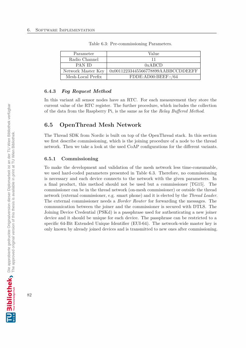
6. Software Implementation
Table 6.3: Pre-commissioning Parameters.
Parameter ValueRadio Channel 11
PAN ID 0xABCDNetwork Master Key 0x00112233445566778899AABBCCDDEEFF
Mesh-Local Prefix FDDE:AD00:BEEF::/64
6.4.3 Fog Request MethodIn this variant all sensor nodes have an RTC. For each measurement they store thecurrent value of the RTC register. The further procedure, which includes the collectionof the data from the Raspberry Pi, is the same as for the Relay Buffered Method.
6.5 OpenThread Mesh NetworkThe Thread SDK from Nordic is built on top of the OpenThread stack. In this sectionwe first describe commissioning, which is the joining procedure of a node to the threadnetwork. Then we take a look at the used CoAP configurations for the different variants.
6.5.1 CommissioningTo make the development and validation of the mesh network less time-consumable,we used hard-coded parameters presented in Table 6.3. Therefore, no commissioningis necessary and each device connects to the network with the given parameters. Ina final product, this method should not be used but a commissioner [TG15]. Thecommissioner can be in the thread network (on-mesh commissioner) or outside the threadnetwork (external commissioner, e.g. smart phone) and it is elected by the Thread Leader.The external commissioner needs a Border Router for forwarding the messages. Thecommunication between the joiner and the commissioner is secured with DTLS. TheJoining Device Credential (PSKd) is a passphrase used for authenticating a new joinerdevice and it should be unique for each device. The passphrase can be restricted to aspecific 64-Bit Extended Unique Identifier (EUI-64). The network-wide master key isonly known by already joined devices and is transmitted to new ones after commissioning.
82

6.5. OpenThread Mesh Network
Table 6.4: Data packet that is sent with CoAP over the Thread network.
Data Byte 0 1 2 3 4 5 6 7 8 9 10 11 12Values NID Value1 Time1 Value2 Time2 Value3 Time3
6.5.2 CoAPThe CoAP protocol is used to manage the transmission of the measurement data. TheCoAP server waits for messages on specific resources and the CoAP client can sendmessages to these resources. We defined three resources: raindrop for the leaf wetness, uvfor the UV and BatteryVoltage for battery voltage. For all variants the relay node has theCoAP server functionality. It is possible to have more than one relay node and thereforemore than one CoAP server. For all variants the sensor nodes send multicast messagesto the CoAP servers. In Fog Request Method (Figure 6.4b) the sensor nodes implementa CoAP server for receiving the get data request. After they received the request, theysend the data like in Forward Only Method and Relay Buffered Method. The data that issent is grouped as shown in Table 6.4. The NID is a unique identifier of the sensors inthe network. The measurement value and the according time are 4 bytes large.
83

6. Software Implementation
(a)
(b)
(c)
Figure 6.5: State machines for the relay node of a) Forward Only Method, b) RelayBuffered Method and c) Fog Request Method.84

CHAPTER 7Validation
The aim of this chapter is to evaluate the self-designed sensors against different criteria.First, the LWS is evaluated and calibrated. After that, the antenna is tested and thepower consumption is examined. Finally, the reliability of the measurements of thesensors in the field tests is revealed. For this purpose, the sensors were mounted in thefield, just as they would be used in a real-life use case.
7.1 LWS Area EvaluationIn this section the LWS is evaluated. This is necessary in order to assign the actual andpossible leaf wetness values to an ADC value.
7.1.1 Comparison of Different PCB TracksIn order to select the most sensitive and separable sensor area for the leaf wetnessmeasurement, the sensors have been tested under different circumstances. Parametersthat have been variated are the frequency of the PWM signal, its duty cycle and the sensetime, which is the time to wait between setting the SENSE_EN to high and taking thefirst measurement value. The sensor surface to be tested is connected to the measuringdevice with a 15cm long cable. The measurement was performed for 4 different wetnessstates: dry, wetted, wet and sprayed. In the dry condition there is no water on thesurface. In the wetted state, half of the area is covered with water and in the wet state,water covers the full area. In the sprayed condition, water was sprayed on the surface, sothere are about 15 small drops on the surface. In Figure 7.1 to 7.4 the results of taking 31samples in an interval of 5 minutes are presented for different parameters and conditions.Each of these measurements was taken for the wetness area with small, medium andlarge PCB tracks. Figure 7.1 b) to 7.4 b) shows the ADC value of the high and lowmeasurements and Figure 7.1 a) to 7.4 a) shows the difference of the high and low value.
85

7. Validation
Table 7.1: Used parameters for comparing different PCB tracks.
Reference PWM frequency [MHz] Duty cycle [%] Sense time [µs]Measurement1 1 25 20Measurement2 0.2 25 20Measurement3 1 50 20Measurement4 1 75 20
Table 7.2: Comparison of the difference from the mean values for different PCB tracks.
Reference PCB Track Difference of the mean valueDry-Sprayed Sprayed-Wetted Wetted-Wet
small 127 114 30medium 121 139 34Measurement1
large 59 198 56small 37 170 148
medium 50 110 110Measurement2large 39 5 145small 124 282 139
medium 219 139 139Measurement3large 33 192 144small 209 271 178
medium 252 164 164Measurement4large 52 183 179
Subtracting the low value from the high value increases the difference between themeasurement values of the different wetness conditions and therefore enables betterseparability. Table 7.1 shows the parameters used for the comparison. For the PWMfrequency 1MHz was chosen because it is the highest frequency which can be generatedby the nRF52840 and the circuit was calculated for this condition. For testing purposesthe frequency was set to 200kHz. Under this circumstance, the separability shown inFigure 7.2 is worse than for 1MHz because it is not possible to make an exact boundarybetween the different wet conditions. To find the best duty cycle, we compared three ofthem. Table 7.2 shows the differences in the mean values of the neighboring moisturestates (Dry-Sprayed, Sprayed-Wetted and Wetted-Wet). A high value in Table 7.2 standsfor a good separability between two wetness states. We want the value for all three states(Dry-Sprayed, Sprayed-Wetted and Wetted-Wet) to be as high as possible. The bestseparability of the different wetness conditions was achieved with a duty cycle of 75%and the small PCB tracks shown in Figure 7.4. The according mean values are markedgreen in Table 7.2.
86

7.1. LWS Area Evaluation
0 10 20 300
200
400
600
800
1,000
Samples
AD
Cva
lue
smal
l
dry wettedwet sprayed
0 10 20 300
200
400
600
800
1,000
Samples
AD
Cva
lue
med
ium
0 10 20 300
200
400
600
800
1,000
Samples
AD
Cva
lue
larg
e
(a)
0 10 20 300
200
400
600
800
1,000
SamplesA
DC
valu
esm
all
0 10 20 300
200
400
600
800
1,000
Samples
AD
Cva
lue
med
ium
0 10 20 300
200
400
600
800
1,000
Samples
AD
Cva
lue
larg
e
(b)
Figure 7.1: Measurement1 for a PWM frequency of 1MHz, a duty cycle of 25% and asense time of 20µs. a) shows the difference of high and low values and b) shows the highand low values of the ADC
87

7. Validation
0 10 20 300
200
400
600
800
1,000
Samples
AD
Cva
lue
smal
ldry wettedwet sprayed
0 10 20 300
200
400
600
800
1,000
Samples
AD
Cva
lue
med
ium
0 10 20 300
200
400
600
800
1,000
Samples
AD
Cva
lue
larg
e
(a)
0 10 20 300
200
400
600
800
1,000
Samples
AD
Cva
lue
smal
l
0 10 20 300
200
400
600
800
1,000
Samples
AD
Cva
lue
med
ium
0 10 20 300
200
400
600
800
1,000
Samples
AD
Cva
lue
larg
e
(b)
Figure 7.2: Measurement2 for a PWM frequency of 200kHz, a duty cycle of 25% and asense time of 20µs. a) shows the difference of high and low values and b) shows the highand low values of the ADC
88

7.1. LWS Area Evaluation
0 10 20 300
200
400
600
800
1,000
Samples
AD
Cva
lue
smal
l
dry wettedwet sprayed
0 10 20 300
200
400
600
800
1,000
Samples
AD
Cva
lue
med
ium
0 10 20 300
200
400
600
800
1,000
Samples
AD
Cva
lue
larg
e
(a)
0 10 20 300
200
400
600
800
1,000
SamplesA
DC
valu
esm
all
0 10 20 300
200
400
600
800
1,000
Samples
AD
Cva
lue
med
ium
0 10 20 300
200
400
600
800
1,000
Samples
AD
Cva
lue
larg
e
(b)
Figure 7.3: Measurement3 for a PWM frequency of 1MHz, a duty cycle of 50% and asense time of 20µs. a) shows the difference of high and low values and b) shows the highand low values of the ADC
89

7. Validation
0 10 20 300
200
400
600
800
1,000
Samples
AD
Cva
lue
smal
ldry wettedwet sprayed
0 10 20 300
200
400
600
800
1,000
Samples
AD
Cva
lue
med
ium
0 10 20 300
200
400
600
800
1,000
Samples
AD
Cva
lue
larg
e
(a)
0 10 20 300
200
400
600
800
1,000
Samples
AD
Cva
lue
smal
l
0 10 20 300
200
400
600
800
1,000
Samples
AD
Cva
lue
med
ium
0 10 20 300
200
400
600
800
1,000
Samples
AD
Cva
lue
larg
e
(b)
Figure 7.4: Measurement4 for a PWM frequency of 1MHz, a duty cycle of 75% and asense time of 20µs. a) shows the difference of high and low values and b) shows the highand low values of the ADC.
90

7.1. LWS Area Evaluation
Table 7.3: Measurement values of the sensor area.
x (ADC value) y (Area) leaf wetness [%]750 0 0650 1 10560 2 20460 3 30420 4 40396 5 50370 6 60349 7 70330 8 80307 9 90269 10 100
7.1.2 Relationship of Leaf Wetness to Digital ValueIn this section we assign a leaf wetness value to a digital value by dividing the sensorsurface into 10 areas of equal size, which were successively covered with water. 0 standsfor no water coverage, between 0 and 1 is the first area, between 1 and 2 is the second areaand so on. The measured value when flooding the first area gives us the value for a 10percent leaf wetness. If we cover the areas one and two, we get the value for a 20 percentleaf wetness. We carry out this measurement until all areas are covered and we reachthe value for a 100 percent leaf wetness. Figure 7.5a illustrates the subdivision of thesensor area for the measurement and Figure 7.5b displays the results. From the resultingcurve we see that the line is not linear. Therefore, we make a linear approximationthat is illustrated in Figure 7.5b. In order to obtain the percentage leaf wetness y fora measured ADC value x, we have to look for the two closest known measuring points(x0, y0) and (x1, y1) from Table 7.3. This procedure is sketched in Figure 7.5b. At theend, we calculate y with the help of equation 7.1.
y = y0(x1 − x) + y1(x − x0)x1 − x0
(7.1)
7.1.3 CalibrationCalibration is necessary if the sensors measure different values for the same environmentalconditions. To determine the deviation between the sensors, 50 measurements were takenfrom four sensors at one-minute intervals for the three states dry, wetted and wet. Theresults are illustrated with box plots in Figure 7.6. To calibrate the sensor, we calculatethe deviation of the median from the reference values in Table 7.3. Each measured valueof the sensor must be corrected by this value. The values to be corrected for the foursensors are presented in Table 7.4.
91

7. Validation
(a)
300 500 7000
5
10
ADC value
Are
asy
x
(x0, y0)
(x1, y1)
(b)
Figure 7.5: Measurement to assign a leaf wetness value to a digital value. a) shows thesubdivision of the sensor area and b) shows the measurement result for the wetted areas.
Table 7.4: Deviation from the reference values for different sensors.
sensor correctionvalue
0 -761 -492 -313 -49
92

7.1. LWS Area Evaluation
0 200 400 600 800 1,000
Sensor 0
Sensor 1
Sensor 2
Sensor 3
(a)
0 200 400 600 800 1,000
Sensor 0
Sensor 1
Sensor 2
Sensor 3
(b)
0 200 400 600 800 1,000
Sensor 0
Sensor 1
Sensor 2
Sensor 3
(c)
Figure 7.6: Box plots for the dry (a), wetted (b) and wet (c) states for the leaf wetnessmeasurement for four sensors.
93

7. Validation
7.1.4 Comparison to Existing SensorsA. Ghobakhlou et al. [GAS15] compare 6 different leaf wetness sensors in his paper,these are Hobby Boards LWS, Campell Scientific 237-L, Decagon Devices LWS, PesslInstruments LWS, Painted Hobby Boards and Painted Campbell 237. To compare oursensors with these 6 sensors, two measurements were made over two days. At first, wecompare the surfaces of our sensor and a real leaf. For this, we simultaneously put thesame amount of water on both surfaces. Second, we measure how long it takes for thesetwo surfaces to dry up. Finally, we have to different periods of time, one for the leaf andone for our sensor. The difference between these two time measurements is 11 minutesand is compared with the other 6 sensors in Figure 7.7. As you can see in Figure 7.7, thesensor built by the author takes as long as the other sensors to dry.
The second measurement compares the measured value of the sensor with the visualobservation of actual wetness on the sensor surface. For this purpose, we wet the sensorand measure the time it takes the sensor surface to dry and the time it takes the measuredvalue to signal a dry surface again. The difference between these two time measurementsis 39 minutes and is compared with the other 6 sensors in Figure 7.7. As you can see inFigure 7.7, the sensor built by the author needs the most time to measure a dry surfaceagain.
7.2 AntennaThe amplitude over the distance of the antenna is measured as shown in Figure 7.8a.For the measurement the nRF Connect software is provided by Nordic. Figure 7.8billustrates the result, the sensor board is placed at different distances away from the nRFUSB Dongle, which is used for the measurement. The z value was fixed at 0.5m. Thefree space path loss behaves as planned in Section 5.2 and corresponds to the referencedesign.
7.3 Power ManagementIn this section the power management is examined under real-life conditions. The solarpanel has a size of about 20 x 20 cm and for the battery a capacity of 1.1Ah was chosen.Under full sunlight the battery was charged in about 1 hour. In Figure 7.10 the PVcharging current under full sunlight is shown. The charging behavior is the same asdescribed in the datasheet of the BQ25895 [Ins18]. The solar panel was placed in a waythat no object can cast a shadow on it. Figure 7.9a shows the solar panel voltage over aperiod of 24 hours and Figure 7.9b shows the battery voltage. For loading the battery aminimum of 4.2V of solar panel voltage is required, this was configured in Section 6.1.7.The measurements were taken in winter in three different weather settings defined bythe International Commission on Illumination (CIE) [CIE]: overcast sky, cloudy sky andclear sky.
94

7.3. Power Management
Hobby
Boards
Campb
ell23
7
Decago
nPess
l
Painted
Hobby
Boards
Painted
Campb
ell23
7
own sen
sor−60−50−40−30−20−10
0102030405060
Mea
nD
elay
[Min
utes
]
Visual observation vs real leavesVisual observation vs sensor reading
Figure 7.7: Comparison of own sensor dry-off against 6 sensor results from A. Ghobakhlouet al. [GAS15].
As we can see from the voltage curve in Figure 7.9a, it is not possible to load on anovercast day and in the other two cases, only at noon because at this point the sun light ishighest and therefore the voltage is higher than 4.2V. The battery voltage measurementhas the precondition that in all cases the battery voltage is the same at the beginning ofthe measurement. The minimum battery voltage is 3.3V and the maximal is 4.2V. Whenthe sky is overcast, the battery voltage decreases by about 9 percent, when the sky iscloudy, it stays the same and when the sky is clear, the voltage increases by about 9percent.
95

7. Validation
(a)
0 5 10 15 20
−80
−60
−40
−20
Distance [m]
Am
plitu
de[d
Bm]
(b)
Figure 7.8: a) shows the setup for the measurement of the amplitude of the antenna andb) shows the result.
0 10 200
2
4
6
Time of day [h]
Sola
rpa
nelv
olta
ge[V
]
Overcast skyCloudy skyClear sky
(a)
0 10 20
3.75
3.8
3.85
3.9
Time of day [h]
Batt
ery
volta
ge[V
]
(b)
Figure 7.9: Solar panel a) and battery b) voltages for different weather conditions.
96

7.3. Power Management
0 1,000 2,000 3,000 4,000
200
400
600
800
Seconds [s]
Cur
rent
[mA
]
Figure 7.10: PV charging current under full sunlight.
97

7. Validation
Table 7.5: Price table of the components for one sensor and relay board.
Type Price [e](09/2019) SellerCapacitors 5.34
From Mouser [Mou]
Resistors 1.9Inductors 0.72Diodes 1.14Crystals 2.02nRF52840 5.45BQ25895 2.85TPS2121 1.81VEML6070 2.36Case 100mmx60mm 6.15Other components 7.34PCB Board 5.9 From JLCPCB [JLC]Assembly 5 Cost estimate from 7pcb
[7PC]9W solar panel 71.75 From Sparkfun [Spa]Battery 1.1Ah 9.04Summary 131.49
7.4 Expenditure on the Board
Table 7.5 lists the prices for the components of a sensor and their sellers. The assemblyis based on a cost estimate because for the small number of 5 prototypes hand solderingis cheaper. The minimum quantity for the listed assembly price is 24 boards and thecomponents must be purchased from the assembler. The total cost of about e131 doesnot meet our requirement of e110, which we have set in Chapter 3.1. But our sensor isstill cheaper than the least inexpensive Waspmote for 240e, which we have compared inChapter 2.
7.5 Field Test
For the field test four sensors were mounted outdoors. The aim was to test the wholenetwork as shown in Figure 4.7. The recorded measured values were the power consump-tion of the relay and sensor node and the reliability of the leaf wetness, UV and batteryvoltage data. Figure 7.11a shows schematically the distances between the sensors. Figure7.11b shows a picture of a mounted sensor in the vineyard, without the case, the solarpanel and the battery installed.
98

7.5. Field Test
(a) (b)
Figure 7.11: Field test setup. a) shows the schematic representation of the deployment ofthe sensors in the field and b) shows the photo of a mounted sensor node in a vineyard.
7.5.1 Power ConsumptionThe used ampere for the sensor and relay node for the three different variants are shownin Figure 7.12. The measurements were taken over a time period of one hour. The sensornodes have taken one measurement every minute.
Forward Only Method The resulting average consumption is 15mA for the sensornode because the data is transmitted every minute immediately after taking the mea-surement and it needs more energy for that process. The relay node consumes 36mA,which is due to the permanent active Bluetooth connection. This is necessary becausethe relay node forwards received data immediately to the fog node.
Relay Buffered Method For this method the fog node collects the data every fiveminutes. Therefore, the relay node has to buffer five measurements for each sensor. Inaverage the sensor node consumes 14.3mA and the relay node 34.5mA. The Bluetoothconnection is active every five minutes.
Fog Request Method For this method the fog node collects the data every five minutes.Therefore, the Bluetooth and Thread connections are only active every five minutes. Inaverage the sensor node consumes 12mA and the relay node 34.5mA.
99

7. Validation
Table 7.6: Comparison of power consumption of our sensor to already existing systems,which were discussed in Chapter 2.
System Node Consumption [mA] Relay/Gateway Consumption [mA]Davis Instruments 12 25
Libelium 17 270Own 15 36
On the one hand the power consumption of the relay node of the Relay Buffered Methodand the Fog Request Method is the same because in both variants they manage the sametasks related to the receiving and sending of the data. On the other hand the sensor nodefor the Relay Buffered Method consumes more power because it sends the data everyminute, whereas for the Fog Request Method the data is sent only every five minutes.
In Chapter 2 we compared existing measurement systems and discussed their powerconsumption. The gateway of the Davis Instruments EnviroMonitor mesh networkconsumes a minimum of 25mA and the node 12mA. The system from Libelium includesthe Waspmote Plug & Sense, which consumes 17mA in the on state and 30µA in thesleep state. The Meshlium consumes 270mA. In Table 7.6 these values are compared tothe power consumption of our sensor with the Forward Only Method. Our sensor nodeconsumes in the on state as much current as other systems. It does not yet have a sleepstate because in a thread network only a certain number of nodes are allowed to go tosleep to prevent the network from being destroyed and this requires further investigationsinto the software implementation. The relay node of our system needs more power thanthat of Davis Instruments but less than the one from Libelium. Our relay node needsthis amount of power because it is waiting for incoming connections from Bluetooth andthe Thread network.
7.5.2 ReliabilityThe reliability of the sensors was measured over a period of two days. Four sensors wereconfigured, so one sensor value is recorded every minute. After that, it was checkedwhether the sensor data arrived correctly at the Raspberry Pi. The percentage evaluationof this measurement for the three different variants is shown in Figure 7.13. Since Threaduses UDP for transmitting data, which is connectionless and non-reliable, data could getlost. For each measurement type there is a separate CoAP resource, these are transmittedseparately. Therefore, it can happen that, e.g. only the UV measurement value is lost ata certain time but leaf wetness and battery voltage reach their destination.
100

7.5. Field Test
Forward Only Method
Relay BufferedMethod
Fog Request Method10
15
20
25
30
35
Con
sum
ptio
n[m
A]
Relay nodeSensor node
Figure 7.12: Average power consumption of the relay and sensor nodes for the threedifferent transmission variants.
Forward Only Method The resulting reliability for the leaf wetness and UV mea-surement is 94%. For the battery voltage measurement it is 90%. With the ForwardOnly Method the thread network is more reliable because the data is sent directly to thefog node after each measurement. In this case the network has smaller intervals betweendata transfers, so the routes in the network and the roles of the nodes remain the samefor a longer time. Since this method is centralized, it is very bad for reliability if a centralnode like the relay node or the fog device fails because all data is lost. But this did nothappen during the test period.
Relay Buffered Method For this method the reliability for the leaf wetness is 87%,for the UV it is 91% and for the battery voltage measurement it is 90%. With thismethod data can be lost if the fog device does not fetch the data from the relay node intime and therefore the ring buffer overflows. In addition, as in the Forward Only Method,data can get lost in the network.
Fog Request Method For this method the reliability for the leaf wetness is 92.4%,for the UV it is 89% and for the battery voltage measurement it is 88.1%. With thismethod, as with Relay Buffered Method, data can get lost if the fog device does not fetchthe data from the sensor nodes in time. Since each sensor stores its own data, it is lesslikely that the buffer will overflow because there is more storage space available.
101

7. Validation
Forward Only Method
Relay BufferedMethod
Fog Request Method86
88
90
92
94
Rel
iabi
lity
[%]
Leaf wetnessUV
Battery voltage
Figure 7.13: Percentage reliability of sensor data from four sensors over a period of 2days.
102
CHAPTER 8Conclusion
The aim of this thesis was to build an IoT sensor swarm for agricultural microclimatemeasurement. For this purpose, a prototype was built to measure the leaf wetness andUV radiation and it was tested for range, reliability and power consumption. The leafwetness sensor imitates a leaf and measures the wetness on the sensor surface withthe help of the change in capacitance. Three leaf wetness areas with different PCBtracks were compared. For transmitting the data, a mesh network was used and threepossible transmission methods were evaluated. The power consumption is as good aswith commercially available products. Nevertheless, there is still and always room forimprovement, also in connection with reliability.
8.1 Outlook and Further Tasks
With this work several aspects were identified that can be improved to get a higher mea-surement reliability and consume less power. The following points should be consideredin further research.
8.1.1 Sensor Manufacturing
The manufacturing of the sensors includes the steps: PCB manufacturing, PCB assembly,ordering all components and end testing. The equipment needed to manufacture thesensors and the companies that can take over steps from the manufacturing shouldalready be analyzed and compared before the start of the development. This has to bedone in order to avoid shortlisting products in the beginning that cannot be assembledlater in the process. In our case, the placement, soldering and testing of the nRF52840should be done by a professional company.
103

8. Conclusion
8.1.2 Power Consumption OptimizationThe power consumption of the sensor node can be further reduced by improving thesource code. This could be done by, for example, compressing the measurement data todecrease the necessary payload when transmitting. This has to be evaluated further bycomparing the necessary power for compression versus the transmission power. Anotherpossibility is to define certain nodes in the thread network as sleepy end devices. Asleepy end device turns off the radio for a predefined time. Afterwards it switches intosleep mode. Each sleepy end device needs a parent which buffers the messages whenit is sleeping. Therefore, a sleeping mode is not intended for the parent. Only a smallnumber of nodes in a thread network can go to sleep because the others have to keep thenetwork running. However, an overall concept of the network to be built up is neededto use the maximum number of sleepy end devices. Another possibility to minimize thepower consumption is to increase the measuring interval.
8.1.3 Increase ReliabilityThe reliability of the measured values can be improved by using check sums duringtransmission. Since Thread uses UDP for transmitting data, which is connectionless andnon-reliable, data could get lost. Further data loss can occur if a sensor runs out of powerand the data is not stored in a non-volatile memory. To prevent the non-volatile memoryfrom overflowing, in addition to the internal flash memory of the nRF52840, an externalflash can be installed. Another aspect to mention is, if the fog node misses any data, itcould request a re-transmission from the sensor or the relay node.
104

CHAPTER 9Appendix
This appendix includes the full schematic of the sensor board.
105

9. Appendix
Figure 9.1: Schematic for the nRF52840.
106

Figure 9.2: Schematic for the leaf wetness measurement.
107

9. Appendix
Figure 9.3: Schematic for the power management.
108

List of Figures
2.1 Different Network Topologies, where the lines illustrate the possible communi-cation paths. The connected nodes can build a Line (a), Mesh (b), Ring (c),Star (d), Bus (e) or a Tree (f). . . . . . . . . . . . . . . . . . . . . . . . . 6
2.2 Schematic of a star and peer-to-peer network topology supported by the IEEE802.15.4 standard [ASA+18]. . . . . . . . . . . . . . . . . . . . . . . . . . . 11
2.3 The superframe structure of the BE Data Link mode of IEEE 802.15.4 standard[ASA+18]. . . . . . . . . . . . . . . . . . . . . . . . . . . . . . . . . . . . . 13
2.4 The mesh networking architecture of Thread [ASA+18]. . . . . . . . . . . 182.5 Scopes of a Thread network [IETe] . . . . . . . . . . . . . . . . . . . . . . 182.6 BR/EDR (a), BLE (b), IEEE 802.15.4 (c) and IEEE 802.11 (d, WLAN)
sharing 2.4GHz frequency band [ASA+18] . . . . . . . . . . . . . . . . . . 202.7 The CS616 [Sci] is a product from Campbell Scientific and is based on the
FDR technique. . . . . . . . . . . . . . . . . . . . . . . . . . . . . . . . . . 222.8 Resistor-based soil moisture sensor board from Sparkfun [Elea]. . . . . . . 222.9 Schematic of resistor and capacitive measurement method. a) shows the
schematic cut through the PCB for the resistor-based measurement and b)for the capacitive-based measurement. . . . . . . . . . . . . . . . . . . . . 23
2.10 Different resistor-based leaf wetness sensors. a) shows the product fromCampbell [Camb], b) shows the product from Davis Instruments [Cor] andc) shows the product from Pessl, which measures the conductance of a filterpaper between two stainless electrodes [Gmbb]. . . . . . . . . . . . . . . 24
2.11 Different capacitive-based leaf wetness sensors. a) shows the product fromCampbell [Cama], b) shows the product from Davis Instruments [Insa] and c)shows the product from Adcon [Adca]. . . . . . . . . . . . . . . . . . . . 25
2.12 Break out board for the VEML6075 by Sparkfun [Eleb]. . . . . . . . . . . 262.13 Sensor Puck from Silicon Labs [Labc]. . . . . . . . . . . . . . . . . . . . . 272.14 Adcon Weather Station [Adcb]. a) is the main part called ADCON RTU. 282.15 Metos Weather Station imt300 [Gmba]. . . . . . . . . . . . . . . . . . . . 292.16 Schematic structure of the EnviroMonitor mesh network [Insb]. . . . . . . 302.17 Waspmote and Waspmote Addons [Lib]. a) shows the hardware board Wasp-
mote, b) shows the Waspmote 802.15.4 radio board, and c) shows the Wasp-mote Agriculture Sensor board, with different sensors. . . . . . . . . . . . . 31
109

2.18 Ready-to-use products from Libelium [Lib]. a) shows the Waspmote Plug &Sense and b) shows the Meshlium 4.0. . . . . . . . . . . . . . . . . . . . . 32
4.1 Different conductor thicknesses to test the moisture sensitivity. a) shows thewetness area with large tracks, b) shows the wetness area with medium tracksand c) shows the wetness area with small tracks. . . . . . . . . . . . . . . 42
4.2 Capacitance measurement with the difference method. . . . . . . . . . . . 424.3 CDC Simplified Block Diagram of the Analog Devices AD7746 [Dev]. . . 434.4 Bode diagram of a first order low pass filter. The green line with cutoff
frequency (f13db) shows the damping of the input signal with a big capacitanceand the blue line (f23db) for a smaller one. The frequency of the input signalis 1MHz ( fin). . . . . . . . . . . . . . . . . . . . . . . . . . . . . . . . . . 44
4.5 Low pass filter circuit. . . . . . . . . . . . . . . . . . . . . . . . . . . . . . 444.6 Capacitor charging and discharging curves in steady state. C1=1nF (dry leaf)
and C2=3nF (wet leaf) . . . . . . . . . . . . . . . . . . . . . . . . . . . . . 454.7 Schematic design of the sensor network. . . . . . . . . . . . . . . . . . . . 474.8 Different transmission possibilities. a) shows the Forward Only Method, b)
shows the Relay Buffered Method and c) shows the Fog Request Method. Thesemicolon-separated list illustrates the following data: "ID of the sensor; Typeof Measurement; Value; Time" . . . . . . . . . . . . . . . . . . . . . . . . 49
4.9 Schematic of the BQ2403x dual input charger IC from Texas Instruments[Ins14]. . . . . . . . . . . . . . . . . . . . . . . . . . . . . . . . . . . . . . 54
4.10 Schematic of the power mux TPS2121 connected to the battery chargerBQ25895. Both components are from Texas Instruments. . . . . . . . . . 54
4.11 Solar Cell IV curve with MPP [Com06]. . . . . . . . . . . . . . . . . . . . 574.12 Photovoltaic power potential in Austria [Sol]. . . . . . . . . . . . . . . . . 59
5.1 Antenna dimensions [Aud08b]. . . . . . . . . . . . . . . . . . . . . . . . . 625.2 Matching network of the antenna. . . . . . . . . . . . . . . . . . . . . . . 635.3 Schematic power flow. . . . . . . . . . . . . . . . . . . . . . . . . . . . . . 635.4 Schematic of the TPS2121 power mux. . . . . . . . . . . . . . . . . . . . . 655.5 Configuration of TPS2121. a) shows the voltage divider for the input source
priority, b) shows the voltage divider for the over voltage protection on VIN1and c) shows the voltage divider for the over voltage protection on VIN2. 66
5.6 Schematic of the BQ25895 battery charger. . . . . . . . . . . . . . . . . . 665.7 Capacitance leaf wetness measurement circuit. . . . . . . . . . . . . . . . 675.8 LWS boards with dimensions for the calculations. a) shows the wetness area
with large tracks, b) shows the wetness area with medium tracks and c) showsthe wetness area with small tracks. . . . . . . . . . . . . . . . . . . . . . . 68
5.9 (a) Top view (b) Cut through view [AM12]. . . . . . . . . . . . . . . . . . 695.10 Capacitor charging voltage differences for resistor values from the E6 table. a)
shows it for the large tracks, b) shows it for the medium tracks and c) showsit for the small tracks. . . . . . . . . . . . . . . . . . . . . . . . . . . . . . 70
5.11 Schematic of the VEML6070 circuit. . . . . . . . . . . . . . . . . . . . . . . 71
110

5.12 PCB layout of the finished board. . . . . . . . . . . . . . . . . . . . . . . 725.13 a) shows the rope clamp to mount the sensor board [dp] and b) shows the
case. . . . . . . . . . . . . . . . . . . . . . . . . . . . . . . . . . . . . . . . 72
6.1 Ring buffer, where the write pointer indicates the next position to be writteninto the memory and the send pointer indicates the value that is transmittednext. . . . . . . . . . . . . . . . . . . . . . . . . . . . . . . . . . . . . . . . 74
6.2 Memory layout for the nRF52840, with a flash size of 1024kB. . . . . . . 756.3 State machine to get a wetness value. . . . . . . . . . . . . . . . . . . . . 776.4 State machines of the main program for the sensor nodes. a) shows the
Forward Only Method and the Relay Buffered Method and b) shows the FogRequest Method. . . . . . . . . . . . . . . . . . . . . . . . . . . . . . . . . 78
6.5 State machines for the relay node of a) Forward Only Method, b) RelayBuffered Method and c) Fog Request Method. . . . . . . . . . . . . . . . . 84
7.1 Measurement1 for a PWM frequency of 1MHz, a duty cycle of 25% and asense time of 20µs. a) shows the difference of high and low values and b)shows the high and low values of the ADC . . . . . . . . . . . . . . . . . . 87
7.2 Measurement2 for a PWM frequency of 200kHz, a duty cycle of 25% and asense time of 20µs. a) shows the difference of high and low values and b)shows the high and low values of the ADC . . . . . . . . . . . . . . . . . . 88
7.3 Measurement3 for a PWM frequency of 1MHz, a duty cycle of 50% and asense time of 20µs. a) shows the difference of high and low values and b)shows the high and low values of the ADC . . . . . . . . . . . . . . . . . . 89
7.4 Measurement4 for a PWM frequency of 1MHz, a duty cycle of 75% and asense time of 20µs. a) shows the difference of high and low values and b)shows the high and low values of the ADC. . . . . . . . . . . . . . . . . . 90
7.5 Measurement to assign a leaf wetness value to a digital value. a) shows thesubdivision of the sensor area and b) shows the measurement result for thewetted areas. . . . . . . . . . . . . . . . . . . . . . . . . . . . . . . . . . . 92
7.6 Box plots for the dry (a), wetted (b) and wet (c) states for the leaf wetnessmeasurement for four sensors. . . . . . . . . . . . . . . . . . . . . . . . . . 93
7.7 Comparison of own sensor dry-off against 6 sensor results from A. Ghobakhlouet al. [GAS15]. . . . . . . . . . . . . . . . . . . . . . . . . . . . . . . . . . 95
7.8 a) shows the setup for the measurement of the amplitude of the antenna andb) shows the result. . . . . . . . . . . . . . . . . . . . . . . . . . . . . . . 96
7.9 Solar panel a) and battery b) voltages for different weather conditions. . . 967.10 PV charging current under full sunlight. . . . . . . . . . . . . . . . . . . . 977.11 Field test setup. a) shows the schematic representation of the deployment of
the sensors in the field and b) shows the photo of a mounted sensor node in avineyard. . . . . . . . . . . . . . . . . . . . . . . . . . . . . . . . . . . . . 99
7.12 Average power consumption of the relay and sensor nodes for the three differenttransmission variants. . . . . . . . . . . . . . . . . . . . . . . . . . . . . . . 101
7.13 Percentage reliability of sensor data from four sensors over a period of 2 days. 102
111

9.1 Schematic for the nRF52840. . . . . . . . . . . . . . . . . . . . . . . . . . 1069.2 Schematic for the leaf wetness measurement. . . . . . . . . . . . . . . . . 1079.3 Schematic for the power management. . . . . . . . . . . . . . . . . . . . . 108
112

Acronyms
BLE Bluetooth Low Energy
NFC Near Field Communication
SoC System on Chip
RTOS Real Time Operating System
IoT Internet of Things
SPOF Single Point of Failure
OSI Open System Interconnection
ISO International Organization for Standardization
HTTP Hypertext Transfer Protocol
FTP File Transfer Protocol
DNS Domain Name System
SSL Secure Sockets Layer
TLS Transport Layer Security
MQTT Message Queuing Telemetry Transport
CoAP Constrained Application Protocol
PPTP Point to Point Tunneling Protocol
UDP User Datagram Protocol
DTLS Datagram Transport Layer Security
TCP Transmission Control Protocol
TLS Transport Layer Security
6LoWPAN IPv6 over Low power Wireless Personal Area Network
IEEE Institute of Electrical and Electronics Engineers
IP Internet Protocol
ARP Address Resolution Protocol
ICMP Internet Control Message Protocol
113

RFCOMM Radio Frequency Communication
SDP Service Discovery Protocol
L2CAP Logical Link Control and Adaptation Protocol
HCI Host Controller Interface
SPF Shortest Path Bridging
EIA Electronic Industries Alliance
SIG Bluetooth Special Interest Group
IETF Internet Engineering Task Force
IEEE-SA Institute of Electrical and Electronics Engineers Standards Association
IPv6 Internet Protocol Version 6
MTU Maximum Transmission Unit
AES Advanced Encryption Standard
CCM Counter with CBC-MAC
WPAN Wireless Personal Area Networks
PAN Personal Area Network
FFD Full Function Device
RFD Reduced Function Device
ISM Industrial, Scientific and Medical
LQI Link Quality Indication
CCA Clear Channel Assessment
ED Energy Detection
DSSS Direct Sequence Spread Spectrum
CSMA Carrier Sense Multiple Access
CA Collison Avoidance
CD Collison Detection
BE Beacon Enabled
NBE Non-Beacon Enabled
114

CAP Contention Access Period
CFP Contention Free Period
TDMA Time Division Multiple Access
BI Beacon Interval
BO Beacon Order
SD Superframe Duration
SO Superframe Order
NSFS Number of Superframe Slots
BSFD Base Super Frame Duration
SP Symbol Period
DVA Distance Vector Algorithm
FTD Full Thread Devices
MTD Minimal Thread Devices
REED Router Eligible End Device
FED Full End Device
MED Minimal End Device
SED Sleepy End Device
NCP Network Coprocessor
GFSK Gaussian Frequency Shift Keying
FHSS Frequency Hopping Spread Spectrum
REST Representational State Transfer
MQTT Message Queuing Telemetry Transport
IBM International Business Machines
OASIS Organization for the Advancement of Structured Information Standards
IPSec Internet Protocol Security
UVA Ultraviolet A
UVB Ultraviolet B
115
UVC Ultraviolet C
FDR Frequency Domain Reflectometry
TDT Time Domain Transmission
TDR Time Domain Reflectometry
UV Ultraviolet Radiation
I2C Inter-Integrated Circuit
PCB Printed Circuit Board
CCD Charge-coupled Device
CMOS Complementary metal-oxide-semiconductor
GSM Global System for Mobile Communications
GPRS General Packet Radio Service
UMTS Universal Mobile Telecommunications System
UHF Ultra-High-Frequency
LoRaWAN Long Range Wide Area Network
Edge Enhanced Data Rates for GSM Evolution
RS232 Recommended Standard 232
2G Second generation mobile network
3G Third generation mobile network
4G Fourth generation mobile network
SDK Software Development Kit
API Application-Programming-Interface
USB Universal Serial Bus
EOS Earth Observation Satellites
OTA Over The Air
SOC State Of Charge
LWD Leaf Wetness Duration
SIM Subscriber Identity Module
116

ADC Analog to Digital Converter
RAM Random Access Memory
IC Integrated Circuit
PWM Pulse Width Modulation
SPI Serial Peripheral Interface
MCU Microcontroller Unit
GPIO General Purpose Input Output
NTC Negative Temperature Coefficient
VPCC Voltage Proportional Current Control
VINDPM Voltage Input Dynamic Power Management
DPPM Dynamic Power Path Management
DPM Dynamic Power Management
MPPT Maximum Power Point Tracking
MPP Maximum Power Point
PPM Power Path Management
mux Multiplexer
Mux Multiplexer
MOSFET Metal Oxide Semiconductor Field Effect Transistor
DC Direct Current
PV Photovoltaic
LWS Leaf Wetness Sensor
CDC Capacitive to Digital Converter
Wh Watt hour
LED Light Emitting Diode
SWD Serial Wire Debug
LDO Low Dropout Regulator
SMD Surface Mounted Device
117

SMA SubMiniature version A
BALUN Balanced Unbalanced Network
DK Development Kit
GUI Graphical User Interface
MBR Master Boot Record
WDT Watchdog Timer
UUID Universally Unique Identifier
RPI Raspberry Pi
CSV Comma Separated Values
RTC Real Time Counter
NTP Network Time Protocol
EUI-64 64-Bit Extended Unique Identifier
CIE International Commission on Illumination
M2M Machine-to-Machine
LAN Local Area Network
WHO World Health Organization
DC/DC Buck regulator
118

List of Tables
1.1 Wavelengths of the different UV types. . . . . . . . . . . . . . . . . . . . . 2
2.1 Comparison of wired and wireless networks [Jha17]. . . . . . . . . . . . . 62.2 Comparison of protocols that define the physical layer for wired networks. 72.3 Stack examples according to the OSI model. Column (a) shows protocols that
are used with Thread. The orange cells are fixed because they are defined inthe Thread standard. Column (b) shows protocols that are used with Ethernet.The blue cells are fixed because they are defined in the Ethernet standard. Inthe book [BS01] the Bluetooth stack, which does not comply with the OSImodel, is correlated with the OSI Layers; this is shown in Column (c). . 9
2.4 IEEE 802.15.4 Frequency bands and channel details. . . . . . . . . . . . . . 112.5 Comparison of CoAP and MQTT [Nai17]. . . . . . . . . . . . . . . . . . . 152.6 Comparison of different Wireless Technologies. . . . . . . . . . . . . . . . 162.7 Different values for r [VTC17]. . . . . . . . . . . . . . . . . . . . . . . . . 242.8 Costs of the Davis Instruments EnviroMonitor [Insb]. . . . . . . . . . . . 30
3.1 Comparison of existing solutions. . . . . . . . . . . . . . . . . . . . . . . . 38
4.1 Comparison of CDC. . . . . . . . . . . . . . . . . . . . . . . . . . . . . . 434.2 Comparison of UV sensor ICs . . . . . . . . . . . . . . . . . . . . . . . . 454.3 Comparison of Bluetooth Mesh and Thread Mesh network [MLPP16]. . . 464.4 Comparison of data storage consumption. The abbreviation for the pick-up
interval is PUI, MI stands for measurement interval, NS means number ofsensors and SD stands for size of data. PUI and MI are measured in secondsand SD in bytes. . . . . . . . . . . . . . . . . . . . . . . . . . . . . . . . . 50
4.5 Comparison of data storage. Data storage (SD) is set to 5 bytes. The pick-upinterval (PUI) is set to one week. The measurement interval (MI) is set toone minute and the number of sensors (NS) is set to ten. . . . . . . . . . . 51
4.6 Comparison of SoCs. . . . . . . . . . . . . . . . . . . . . . . . . . . . . . . 524.7 Comparison of single and dual input charger ICs. . . . . . . . . . . . . . . 554.8 Comparison of power muxes available on the market. . . . . . . . . . . . . 554.9 Current consumption of nRF52840 [Sem16]. . . . . . . . . . . . . . . . . . 574.10 Overall current consumption, in battery mode. . . . . . . . . . . . . . . . 584.11 Comparison of rechargeable batteries [Mor12]. . . . . . . . . . . . . . . . . 58
119

4.12 Comparison of different antenna types [Aud08a]. . . . . . . . . . . . . . . 60
5.1 Antenna dimensions [Aud08b]. . . . . . . . . . . . . . . . . . . . . . . . . 625.2 Common parameters for the capacitor calculation. . . . . . . . . . . . . . 695.3 Distinctive parameters for the capacitor calculation for each board. . . . . 695.4 Results of the capacitance calculation for the three different boards. . . . 70
6.1 Data packet that is sent with BLE to the subscribed fog device. . . . . . . 806.2 Example of a time stamp calculation for five measurement values. The
calculation is done by the Raspberry Pi and is based on the RTC and the timestamp from the NTP. The outcome are time stamps for each measurementvalue. . . . . . . . . . . . . . . . . . . . . . . . . . . . . . . . . . . . . . . . 81
6.3 Pre-commissioning Parameters. . . . . . . . . . . . . . . . . . . . . . . . . 826.4 Data packet that is sent with CoAP over the Thread network. . . . . . . 83
7.1 Used parameters for comparing different PCB tracks. . . . . . . . . . . . 867.2 Comparison of the difference from the mean values for different PCB tracks. 867.3 Measurement values of the sensor area. . . . . . . . . . . . . . . . . . . . . . 917.4 Deviation from the reference values for different sensors. . . . . . . . . . 927.5 Price table of the components for one sensor and relay board. . . . . . . . 987.6 Comparison of power consumption of our sensor to already existing systems,
which were discussed in Chapter 2. . . . . . . . . . . . . . . . . . . . . . . 100
120

Bibliography
[7PC] 7PCB. 7pcb, a pcb assembler. URL: https://www.7pcb.com/. [Online;last accessed: 2019-09-05].
[AAB+10] D. Allan, P. Ashwood-Smith, N. Bragg, J. Farkas, D. Fedyk, M. Ouellete,M. Seaman, and P. Unbehagen. Shortest path bridging: Efficient control oflarger ethernet networks. IEEE Communications Magazine, 48(10):128–135,October 2010.
[Adca] Adcon. Adcon capacitive leaf wetness sensor. URL:https://www.adcon.com/products/sensors-284/wet-leaf-wetness-sensor-1759/. [Online; last accessed: 2019-09-05].
[Adcb] Adcon. Adcon weather station for agriculture. URL: https://www.adcon.com/solutions/precision-farming-99/. [Online; last ac-cessed: 2019-09-05].
[AGM+15] A. Al-Fuqaha, M. Guizani, M. Mohammadi, M. Aledhari, and M. Ayyash.Internet of things: A survey on enabling technologies, protocols, and appli-cations. IEEE Communications Surveys Tutorials, 17(4):2347–2376, 2015.
[ahd19] ahdb. Satellites for agriculture. URL: https://ahdb.org.uk/knowledge-library/satellites-for-agriculture, 2019. [On-line; last accessed: 2019-09-05].
[AM12] N. Angkawisittpan and T. Manasri. Determination of sugar content in sugarsolutions using interdigital capacitor sensor. Measurement Science Review,12:8–13, 03 2012.
[Ann92] S. Ann. Ultraviolet radiation and plants: Burning questions. The Plant cell,4:1353–1358, 12 1992.
[ASA+18] N. Ali, R. Saleem, P. Angelina, G. Mesut, and D. Behnam. Low-powerwireless for the internet of things: Standards and applications. IEEE Access,PP:1–1, 11 2018.
121

[Aud08a] A. Audun. Selecting antennas for low-power wireless applications. URL:http://www.ti.com/lit/an/slyt296/slyt296.pdf, 2008. [On-line; last accessed: 2019-09-05].
[Aud08b] A. Audun. Small size 2.4 ghz pcb antenna. URL: http://www.ti.com/lit/an/swra117d/swra117d.pdf, 2008. [Online; last accessed: 2019-09-05].
[Awt97] D. Awtrey. Transmitting data and power over a one-wire bus. AppliedSensing Technology, 1997.
[Awt98] D. Awtrey. The 1-wire weather station. SENS(PETERBOROUGH, NH),15(6):34, 1998.
[Bau08] K. Bauer. Weinbau. AV-Fachbuch. Österreichischer Agrarverlag, 2008.
[BKK+08] G. Bleyer, H.H. Kassemeyer, R. Krause, O. Viret, and W. Siegfried. „vitime-teo plasmopara“ – prognosemodell zur bekämpfung von plasmopara viticola(rebenperonospora) im weinbau. Gesunde Pflanzen, 60:91–100, 09 2008.
[BLSa] BLSIG. Bluetooth low energy mesh faq. URL: https://www.bluetooth.com/bluetooth-technology/topology-options/le-mesh/mesh-faq/. [Online; last accessed: 2019-09-05].
[BLSb] BLSIG. Bluetooth special interest group. URL: https://www.bluetooth.com. [Online; last accessed: 2019-09-05].
[BS01] J. Bray and C. F. Sturman. Bluetooth 1.1: Connect without cables, 2nd edi-tion. URL: http://www.informit.com/articles/article.aspx?p=27591&seqNum=5, 2001. [Online; last accessed: 2019-09-05].
[Cama] Campbell. Campbell scientific capacitive leaf wetness sensor. URL: https://www.campbellsci.com/lws. [Online; last accessed: 2019-09-05].
[Camb] Campbell. Campbell scientific resistor based leaf wetness sensor. URL:https://www.campbellsci.com/237-l. [Online; last accessed: 2019-09-05].
[CCC51] D. Croney, J. D. Coleman, and E. W. H. Currer. The electrical resistancemethod of measuring soil moisture. British Journal of Applied Physics,2(4):85–91, apr 1951.
[cco99] ccontrols. Understanding eia-485 networks. Springer 1999 - theExtension, 1,1999. [Online; last accessed: 2019-09-05].
[CIE] CIE. International commission on illumination . URL: http://cie.co.at/. [Online; last accessed: 2019-09-05].
122

[Com06] Wikimedia Commons. Solar cell iv curve with mp.URL: https://commons.wikimedia.org/wiki/File:Solar-Cell-IV-curve-with-MPP.png, 2006. [Online; last ac-cessed: 2019-09-05].
[Cop] R. Coppen. Oasis. URL: https://www.oasis-open.org/committees/tc_home.php?wg_abbrev=mqtt. [Online; last accessed:2019-09-05].
[Cor] Davis Instruments Corporation. Davis instruments resistor based leaf wet-ness sensor. URL: https://www.davisinstruments.com/product/leaf-wetness-sensor-vantage-pro-and-vantage-pro2/. [On-line; last accessed: 2019-09-05].
[CTGD09] F. Chen, T. Talanis, R. German, and F. Dressler. Real-time enabled ieee802.15.4 sensor networks in industrial automation. IEEE InternationalSymposium on Industrial Embedded Systems., pages 136–139, 2009.
[Dav10] A. Davide. Battery Management Systems for Large Lithium Ion BatteryPacks. EBL-Schweitzer. Artech House, 2010.
[Deb18] Open On-Chip Debugger. Open on-chip debugger. URL: http://openocd.org/, 2018. [Online; last accessed: 2019-09-05].
[Dev] Analog Devices. Analog devices ad7746, 24-bit, 2 channel capacitanceto digital converter. URL: https://www.analog.com/en/products/ad7746.html. [Online; last accessed: 2019-09-05].
[Dif02] B. L. Diffey. Sources and measurement of ultraviolet radiation. Methods,28(1):4 – 13, 2002.
[Dif13] B.L. Diffey. Radiation Measurement in Photobiology. Elsevier Science, 2013.
[DIN15] DIN. Preferred number series for resistors and capacitors (iec 60063:2015).URL: https://www.beuth.de/de/norm/din-en-60063/240741276, 2015. [Online; last accessed: 2019-09-05].
[Dja19] W. Djatmiko. Capacitance measurements system using rc circuit. KnESocial Sciences, 3:603, 03 2019.
[dp] dq pp. Mounting rope clamp. URL: http://dq-pp.com/stainless-steel-bolt-clip-from-pieces-p-6994.html. [On-line; last accessed: 2019-09-05].
[Elea] SparkFun Electronics. Sparkfun soil moisture board. URL: https://www.sparkfun.com/products/13322. [Online; last accessed: 2019-09-05].
123

[Eleb] SparkFun Electronics. Veml6075 break out board. URL: https://www.sparkfun.com/products/15089. [Online; last accessed: 2019-09-05].
[FJ94] Z. Fedro and X. Jiannong. Soil moisture sensors 1. Bulletin292, 1994.
[Fou] Python Software Foundation. Python programming language. URL: https://www.python.org/. [Online; last accessed: 2019-09-05].
[fSI94] International Organization for Standardization (ISO). Information tech-nology - open systems interconnection - basic reference model: The basicmodel. ISO/IEC 7498-1, 1994.
[GAS15] A. Ghobakhlou, F. Amir, and P. Sallis. Leaf wetness sensors - a comparativeanalysis. In 9th International Conference on Sensing Technology (ICST),pages 420–424, 12 2015.
[Gmba] Pessl Instruments GmbH. imetos weather station for agriculture. URL:http://metos.at/de/imetos33/. [Online; last accessed: 2019-09-05].
[Gmbb] Pessl Instruments GmbH. Metos pessl instruments resistor based leaf wet-ness sensor. URL: https://metos.at/portfolio/leaf-wetness/.[Online; last accessed: 2019-09-05].
[Goo] Google. Open thread. URL: https://openthread.io/. [Online; lastaccessed: 2019-09-05].
[Gro] Thread Group. Thread group. URL: https://www.threadgroup.org/thread-group#OurMembers. [Online; last accessed: 2019-09-05].
[Gup13] N. Gupta. Inside Bluetooth Low Energy. Artech House Remote SensingLibrary. Artech House, 2013.
[GYYL09] K. Gill, S.-H. Yang, F. Yao, and X. Lu. A zigbee-based home automationsystem. IEEE Trans. Consum. Electron, 55:422–430, 2009.
[Her13] K.H. Hermann. Der Photoeffekt: Grundlagen der Strahlungsmessung.Vieweg+Teubner Verlag, 2013.
[Hol02] F. Hollósy. Effects of ultraviolet radiation on plant cells. Micron, 33(2):179– 197, 2002.
[HP07] K.K. Hamamatsu Photonics. PHOTOMULTIPLIER TUBES Basics andApplications. Hamamatsu Photonics K.K. Electron Tube Division, 2007.
[HRG18] C. Hirsch, M. Redl, and R. Grosu. Towards an agricultural iot-infrastructurefor micro-climate measurements. Talk: Workshop on Smart Farming, Porto,Portugal, 2018.
124

[IEEa] IEEE. Ieee 802.3. URL: http://www.ieee802.org/3/. [Online; lastaccessed: 2019-09-05].
[IEEb] IEEE. Ieee 802.3-2018 - ieee standard for ethernet. URL: https://standards.ieee.org/standard/802_3-2018.html. [Online; lastaccessed: 2019-09-05].
[IEEc] IEEE. IEEE standard association. URL: http://standards.ieee.org.[Online; last accessed: 2019-09-05].
[IEE12] IEEE Standard for Local and Metropolitan Area Networks—Part 15.4:Low-Rate Wireless Personal Area Networks (LR-WPANs) Amendment 1:MAC Sublayer, IEEE standard 802.15.4e-2012 (amendment to ieee standard802.15.4-2011). pages 1–225, 2012.
[IETa] IETF. The internet engineering task force (IETF). URL: https://www.ietf.org. [Online; last accessed: 2019-09-05].
[IETb] IETF. Rfc4291. URL: https://tools.ietf.org/html/rfc4291.[Online; last accessed: 2019-09-05].
[IETc] IETF. Rfc6282. URL: https://tools.ietf.org/html/rfc6282.[Online; last accessed: 2019-09-05].
[IETd] IETF. Rfc7252. URL: https://tools.ietf.org/html/rfc7252.[Online; last accessed: 2019-09-05].
[IETe] IETF. Thread scope. URL: https://openthread.io/guides/thread-primer/ipv6-addressing. [Online; last accessed: 2019-09-05].
[Ily13] G. Ilya. Making the web faster with http 2.0. Communications of the ACM,56(12):42–49, December 2013.
[Inca] Digi International Inc. Digimesh. URL: https://www.digi.com/products/tag/digimesh. [Online; last accessed: 2019-09-05].
[Incb] Silicon Laboratories Inc. Thread mesh network performance. URL: https://www.silabs.com/documents/login/application-notes/an1141-thread-mesh-network-performance.pdf. [Online; lastaccessed: 2019-09-05].
[Insa] Davis Instruments. Davis instruments capacitive leaf wetness sensor. URL:https://www.davisinstruments.com/. [Online; last accessed: 2019-09-05].
125

[Insb] Davis Instruments. Enviromonitor. URL:https://www.davisinstruments.com/solution/enviromonitor-affordable-field-monitoring-system/.[Online; last accessed: 2019-09-05].
[Ins14] Texas Instruments. Bq2403x. URL: http://www.ti.com/lit/ds/symlink/bq24038.pdf?keyMatch=BQ2403X&tisearch=Search-EN-everything, 2014. [Online; last accessed: 2019-09-05].
[Ins18] Texas Instruments. Datasheet of the bq25895 i2c controlled single cell 5-afast charger with maxchargetm for high input voltage and adjustable voltage3.1-a boost operation. URL: http://www.ti.com/lit/ds/symlink/bq25895.pdf, 2018. [Online; last accessed: 2019-09-05].
[Ins19] Texas Instruments. Datasheet of the tps212x 2.8-v to 22-v priority powermux with seamless switchover. URL: http://www.ti.com/lit/ds/symlink/tps2120.pdf, 2019. [Online; last accessed: 2019-09-05].
[Jaf14] T. Jaffey. Mqtt and coap, iot protocols. URL: https://www.eclipse.org/community/eclipse_newsletter/2014/february/article2.php, 2014. [Online; last accessed: 2019-09-05].
[Jha17] H. Jha. A study and comparison of wired, wireless and optical networks.5:13109 – 13128, 2017.
[JLC] JLCPCB. Jlcpcb, a pcb manufacturer. URL: https://jlcpcb.com/.[Online; last accessed: 2019-09-05].
[JVR+19] P. Jitender, C. Vivek, P. Rishi, C. Sushabhan, M. Ranjan, M. Raj Gaurav,and K. Adesh. A review: Soil moisture estimation using different tech-niques. In Intelligent Communication, Control and Devices, pages 105–111,Singapore, 2019. Springer Singapore.
[KBD+99] U. Karsten, K. Bischof, H. Dieter, H. Tüg, and C. Wiencke. The effect ofultraviolet radiation on photosynthesis and ultraviolet-absorbing substancesin the endemic arctic macroalga devaleraea ramentacea (rhodophyta). Phys-iologia Plantarum, 105:58 – 66, 01 1999.
[KC14] P. Karunakar and A. Chitneni. A comparative study of wireless protocols:Bluetooth, uwb, zigbee, and wi-fi. Advance in Electronic and ElectricEngineering, 4:655–662, 09 2014.
[KiC] KiCad. Kicad eda, a cross platform and open source electronics design au-tomation suite. URL: https://kicad-pcb.org/. [Online; last accessed:2019-09-05].
126

[KK19] A. Khanna and S. Kaur. Evolution of internet of things (iot) and itssignificant impact in the field of precision agriculture. Computers andElectronics in Agriculture, 157:218 – 231, 2019.
[KM14] N. Kaur and S. Monga. Comparisons of wired and wireless networks: areview. International Journal of Advanced Engineering Technology, 5(2):34 –35, 2014.
[LA16] D. Lechner and O. Aceña. Gattlib, python library to use the gatt protocol forbluetooth le devices. URL: https://github.com/ev3dev/gattlib,2016. [Online; last accessed: 2019-09-05].
[Laba] National Renewable Energy Laboratory. Solar cell efficiency. URL: https://pvdpc.nrel.gov/. [Online; last accessed: 2019-09-05].
[Labb] Descartes Labs. Descartes labs. URL: https://www.descarteslabs.com/. [Online; last accessed: 2019-09-05].
[Labc] Silicon Labs. Sensor puck. URL: https://www.silabs.com/products/development-tools/sensors/environmental-biometric-sensor-puck-starter-kit. [Online;last accessed: 2019-09-05].
[LGL+] J.D. Longstreth, F.R. de Gruijl, J.C. van der Leun, M. L Kripke, andY. Takizawa. Effects of increased solar ultraviolet radiation on humanhealth. Ambio, 24.
[Lib] Libelium. Libelium waspmote. URL: http://www.libelium.com/products/waspmote/. [Online; last accessed: 2019-09-05].
[Lim] Arm Limited. Mbedos. URL: https://os.mbed.com/docs/mbed-os/v5.14/reference/thread-tech.html. [Online; last accessed: 2019-09-05].
[LL15] I. Lee and K. Lee. The internet of things (iot): Applications, investments,and challenges for enterprises. Business Horizons, 58(4):431 – 440, 2015.
[LLC] SEGGER Microcontroller Systems LLC. Segger j-link. URL: https://www.segger.com/products/debug-probes/j-link/. [Online; lastaccessed: 2019-09-05].
[MFP+16] V. Montone, C.W. Fraisse, N.A. Peres, P.C. Sentelhas, M. Gleason, M. Ellis,and G. Schnabel. Evaluation of leaf wetness duration models for operationaluse in strawberry disease-warning systems in four us states. InternationalJournal of Biometeorology, 60(11):1761–1774, Nov 2016.
127

[MLPP16] J. Morales, N. A. Lopez, J. Parado, and J. Pasaoa. A comparative study ofthread against zigbee, z-wave, bluetooth, and wi-fi as a home-automationnetworking protocol., 11 2016.
[MLS12] H. Mittelbach, I. Lehner, and S. I. Seneviratne. Comparison of four soilmoisture sensor types under field conditions in switzerland. Journal ofHydrology, 430-431:39 – 49, 2012.
[Mon13] V.O. Montone. Leaf Wetness Duration Modeling and Spatialization toOptimize Fungicide Application in Strawberry Production Systems. Universityof Florida Digital Collections. University of Florida, 2013.
[Mor12] M. Morris. Comparison of rechargeable battery technologies. ASME EarlyCareer Technical Journal, 11:148–155, 11 2012.
[Mou] Mouser. Mouser, a electronic component seller. URL: https://www.mouser.at/. [Online; last accessed: 2019-09-05].
[MPB+16] B. Milija, S. Petar, K. Bozo, Ð. Slobodan, and P. Tomo. A private iot cloudplatform for precision agriculture and ecological monitoring. Computers andElectronics in Agriculture, 140:255 – 265, 06 2016.
[MRC+17] Y. Murillo, B. Reynders, A. Chiumento, S. Malik, P. Crombez, and S. Pollin.Bluetooth now or low energy: Should ble mesh become a flooding or connec-tion oriented network? In 2017 IEEE 28th Annual International Symposiumon Personal, Indoor, and Mobile Radio Communications (PIMRC), pages1–6, 2017.
[Nai17] N. Naik. Choice of effective messaging protocols for iot systems: Mqtt,coap, amqp and http. In 2017 IEEE International Systems EngineeringSymposium (ISSE), pages 1–7, Oct 2017.
[Nin12] J. Ning. Adi capacitance-to-digital converter tech-nology in healthcare applications. URL: https://www.analog.com/en/analog-dialogue/articles/capacitance-to-digital-converter-technology-healthcare.html, 2012. [Online; last accessed: 2019-09-05].
[OBL+15] R. Ojo, P. R. Bullock, J. L’Heureux, Powers, H.J. McNairn, and A. Pacheco.Calibration and evaluation of a frequency domain reflectometry sensor forreal-time soil moisture monitoring. The Soil Science Society of America,Inc., 2015.
[PAM17] N. Poursafar, M. E. E. Alahi, and S. Mukhopadhyay. Long-range wirelesstechnologies for iot applications: A review. In 2017 Eleventh InternationalConference on Sensing Technology (ICST), pages 1–6, 2017.
128

[Pan13] K. Pandya. Network structure or topology. International Journal of AdvanceResearch in Computer Science and Management Studies, 1:22 – 27, 2013.
[PDHM14] R. Priyanka, S. K. Deep, C. Hakima, and B. Marie. Wireless sensor networks:a survey on recent developments and potential synergies. The Journal ofSupercomputing, 68(1):1 – 48, 2014.
[PRSBR17] J. Prasanth Ram, T. Sudhakar Babu, and N. Rajasekar. A comprehensivereview on solar pv maximum power point tracking techniques. Renewableand Sustainable Energy Reviews, 67:826 – 847, 2017.
[RSPAM19] A. K. Rêgo Segundo, E. Pinto, G. Almeida, and P. Monteiro. Capacitiveimpedance measurement: Dual-frequency approach. Sensors, 06 2019.
[San14] L. Sanchez. Smartsantander: Iot experimentation over a smart city testbed.Computer Networks, 61:217–238, 2014.
[SBV+19] A. Singh, A. Bhardwaj, CL. Verma, VK. Mishra, A. Singh, S. Arora,N. Sharma, and R. Ojha. Soil moisture sensing techniques for schedulingirrigation. Journal of Soil Salinity and Water Quality, 11(1):68 – 76, 2019.
[Sci] Campbell Scientific. Cs616 capacitive soil measurement board. URL:https://www.campbellsci.de/cs616-reflectometer. [Online;last accessed: 2019-09-05].
[Sem] Nordic Semiconductor. Nordic nrfjprog. URL: https://www.nordicsemi.com/Software-and-tools/Development-Tools/nRF-Command-Line-Tools. [Online; last accessed: 2020-11-22].
[Sem16] Nordic Semiconductor. Datasheet of the nrf52840. URL: https://infocenter.nordicsemi.com/pdf/nRF52840_OPS_v0.5.pdf,2016. [Online; last accessed: 2019-09-05].
[Sem18a] Nordic Semiconductor. Nordic memory layout libraries. URL: https://infocenter.nordicsemi.com/index.jsp?topic=%2Fcom.nordic.infocenter.sdk5.v15.2.0%2Flib_bootloader.html,2018. [Online; last accessed: 2019-09-05].
[Sem18b] Nordic Semiconductor. Nordic multiprotocol.URL: https://www.nordicsemi.com/Products/Low-power-short-range-wireless/Multiprotocol, 2018. [On-line; last accessed: 2019-09-05].
[Sem18c] Nordic Semiconductor. Nordic softdevice s140. URL: https://infocenter.nordicsemi.com/pdf/S140_SDS_v1.1.pdf, 2018.[Online; last accessed: 2019-09-05].
129

[Sem19] Vishay Semiconductors. Datasheet of the veml6070 uva light sensor with i2cinterface. URL: https://www.vishay.com/docs/84277/veml6070.pdf, 2019. [Online; last accessed: 2019-09-05].
[Sem20] Nordic Semicondutor. nrf52840 development kit. URL: https://infocenter.nordicsemi.com/index.jsp?topic=%2Fug_nrf52840_dk%2FUG%2Fnrf52840_DK%2Fgetting_started.html,2020. [Online; last accessed: 2020-11-22].
[Sho] Farm Shots. Farm shots. URL: http://farmshots.com/. [Online; lastaccessed: 2019-09-05].
[SKB18] S. Sen, J. Koo, and S. Bagchi. Trifecta: Security, energy efficiency, andcommunication capacity comparison for wireless iot devices. IEEE InternetComputing, 22(1):74–81, 2018.
[SMG04] P. Sentelhas, J.E.B.A. Monteiro, and T.J. Gillespie. Electronic leaf wet-ness duration sensor: Why it should be painted. International journal ofbiometeorology, 48:202–5, 06 2004.
[Sol] Solargis. Solargis map for austria. URL: https://solargis.com/maps-and-gis-data/download/austria. [Online; last accessed:2019-09-05].
[Sol18] Low Power Radio Solutions. 2.4ghz compressed stubby / whip an-tenna. URL: https://lprs.co.uk/assets/files/downloads/ant-ss24g-antenna-datasheet-v1.5.pdf, 2018. [Online; last ac-cessed: 2019-09-05].
[Spa] Sparkfun. Sparkfun, a electronic component seller. URL: https://www.sparkfun.com/. [Online; last accessed: 2019-09-05].
[SPS+12] B. Sameer, A. Paventhan, A. Salkrishna, V. Gayathri, and R. N.Mohan.Leveraging coap towards monitoring agriculture sensor network. WirelessCommunication and Sensor Networks, 12 2012.
[SSS+06] C. Sicora, A. Szilárd, L. Sass, E. Turcsányi, Z. Máté, and I. Vass. UV-Band UV-A Radiation Effects on Photosynthesis at the Molecular Level, pages121–135. 07 2006.
[Staa] RFC Internet Standard. Transmission control protocol. URL: https://tools.ietf.org/html/rfc793. [Online; last accessed: 2019-09-05].
[Stab] RFC Internet Standard. User datagram protocol. URL: https://tools.ietf.org/html/rfc768. [Online; last accessed: 2019-09-05].
[Ste16] H. Stefan. Heimautomation mit knx, dali, 1-wire und co. RheinwerkComputing, 2016.
130

[SWA13] M. Shiraz, Md. Whaiduzzaman, and G. Abdullah. A study on anatomyof smartphone. Journal of Computer Communication and Collaboration,1:24–31, 06 2013.
[TG15] Inc Thread Group. Thread commissioning. URL: https://www.threadgroup.org/Portals/0/documents/support/CommissioningWhitePaper_658_2.pdf, 2015. [Online; last accessed:2019-09-05].
[TGL+07] F. Tang, M. Guo, M. Li, Y. Yang, D. Zhang, and Y. Wang. Wirelessmesh sensor networks in pervasive environment: a reliable architecture androuting protocol. In 2007 International Conference on Parallel ProcessingWorkshops (ICPPW 2007), pages 72–72, Sep. 2007.
[Upt19] E. Upton. Raspberry pi specification. URL: https://www.raspberrypi.org/blog/raspberry-pi-4-on-sale-now-from-35/, 2019. [On-line; last accessed: 2019-09-05].
[Vit] Vitimeteo. Vitimeteo - forecasting models, weather data and monitoring forviticulture. URL: https://www.vitimeteo.at/. [Online; last accessed:2019-09-05].
[VTC17] P. Vosoughi, P. Taylor, and H. Ceylan. Impacts of internal curing on theperformance of concrete materials in the laboratory and the field. INTRANSPROJECT REPORTS, 11 2017.
[W3C] World Wide Web Consortium W3C. W3c - http. URL: https://www.w3.org/Protocols/. [Online; last accessed: 2019-09-05].
[Wil11] B. Will. Time domain transmission sensors for soil moisture measurements.In Proceedings of the 19th Telecommunications Forum (TELFOR), pages16–19, 2011.
[YKX+17] Y. Liu, K. Tong, X. Qiu, Y. Liu, and X. Ding. Wireless mesh networks in iotnetworks. In 2017 International Workshop on Electromagnetics: Applicationsand Student Innovation Competition, pages 183–185, May 2017.
[Zig] ZigBee. ZigBee. URL: http://www.zigbee.org. [Online; last accessed:2019-09-05].
131