iot latency and power consumption -...

IoT Latency and Power consumption

PAPER WITHIN Computer Science

AUTHOR: Alexander Lagerqvist, Tejas Lakshminarayana

TUTOR: Rob Day

JÖNKÖPING 2018-05-07

Measuring the performance impact of MQTT and CoAP

This exam work has been carried out at the School of Engineering in Jönköping

in the subject area computer science. The work is a part of the two-year

university diploma of the Master of Science program.

The authors take full responsibility for opinions, conclusions and findings

presented.

Examiner: Anders Adlemo

Supervisor: Rob Day

Scope: 30 credits (second cycle)

Date: 2018-05-07

2

Summary

The purpose of this thesis is to investigate the impact on latency and power consumption of certain usage environments for selected communication protocols that have been designed for resource constrained usage. The research questions in this thesis is based on the findings in Lindén report “A latency comparison of IoT protocols in MES” and seeks to answer the following:

1. ”How does MQTT impact the latency and power consumption on a constrained device?” 2. ”How does CoAP impact the latency and power consumption on a constrained device?” 3. ”How does usage environment influence the latency for MQTT and CoAP?”

This thesis only seeks to explore concepts and usage environments related to wireless sensor networks, internet of things and constrained devices. The experiments have been carried out on a ESP WROOM 32 Core board V2 applying MQTT and CoAP as the communication protocols.

The overall research method used in this thesis is the experimental research design proposed by Wohlin et al. Experiments have been created to support or disprove hypotheses which are formulated to answer the research questions. The experiments were conducted in test environments, which mimic a real-life wireless sensor network environment. The process is thoroughly recorded to further increase the traceability of this thesis. This decision was made due to a comment Boyle et al. made about the problems with real-life experiments about the wireless communication-based research domain. Where Boyle et al. states that there is “insufficient knowledge” available for the research community.

The MQTT related latency experiments showed that QoS level 0 had the lowest latency of all the QoS levels. However, the results also showed that QoS 1 and 2 almost had an identical latency. The CoAP related latency experiments did not indicate any obvious trends. The results from the power consumption related experiments were inconclusive since the data was incomplete.

The usage environment related experiments yielded conclusive results. The data showed that there was a small variation in the latency impact across the various usage environments. Furthermore, the data suggest that CoAP and MQTT had lower latencies in a high signal strength environment compared to a lower signal strength environment. However, it is not clear if there were any unknown factors influencing the results.

Keywords

Internet of things, IoT, Wireless sensor networks, WSN, Constrained devices, MQTT, CoAP, Latency, Power consumption, Experiment

3

Acknowledgements

The authors of this thesis would like to express their gratitude towards the people who contributed to this thesis. Rob Day – For providing invaluable feedback, suggestions and mentoring throughout the thesis. Joakim Gustafsson – For providing invaluable feedback and suggestions about the experiment phase and helping the authors to setup the experiment environment. Sergio Lara – For providing feedback and suggestions about the research problem as well as domain expertise.

4

List of abbreviations

AMQP - Advanced Message Queuing Protocol

BLE - Bluetooth Low Energy

CoAP - Constrained Application Protocol

ESP 32 - ESP WROOM 32 Core board V2

GPIO - General-purpose input/output

HTTP - Hypertext Transfer Protocol

IETF - Internet Engineering Task Force

IoT - Internet of Things

lwIP - lightweight Internet Protocol

MES - Manufacturing Execution System

Mote - Sensor node

MQTT - Message Queue Telemetry Transport

ms - milliseconds

mV - millivolt

NTP - Network Time Protocol

QoS - Quality of Service

REST - Representational State Transfer

Sink, hub - Gateway

SNTP - Simple Network Time Protocol

TCP - Transmission Control Protocol

UDP - User Datagram Protocol

WSN - Wireless Sensor Network

5

Glossary

Communication protocol – A communication protocol is a software technology that enable or influence data communication of a device.

Constrained Device – A constrained device (also known as a resource constrained device) is a device that is limited in terms of energy, computational power, memory or storage capabilities. A constrained device may use sleep mode (low-energy mode) to decrease its power consumption.

Connectivity performance – Connectivity performance is an umbrella term that describes the impact on quality aspects that is related to a communication or a message transaction, these aspects involve latency, throughput, error rate, package loss and jitter. This thesis is focused on the latency aspect of connectivity performance.

Power consumption – Power consumption means the amount of electrical power used for an activity or period, for an electricity powered device.

Gateway – The gateway is the hub in a WSN, which receives data from one or more sensor nodes. The purpose of a gateway is to relay the data to a service or server that is outside of the WSN’s network.

Latency – Latency is used to describe the delay from when a message is sent and when it is received.

Message – A message is a package of data that is going to be sent in a message transaction.

Message transaction – Message transaction is a communication between two devices, which involves the sending and reception of messages or packages.

Message size – Message size (also known as payload size) describe the size of a data package (a message) that is being sent to a device.

Payload – Payload is a synonym for message.

Sensor node – A sensor node is a device which has one or more sensors on it. The sensor node sends its data to the gateway.

Usage environment – A usage environment describes the environment in which a device is deployed in and the variables of the environment. Usage environment can describe: the interference, signal strength, moisture, temperature and such for the environment it describes. In this thesis, usage environments are used as a variable for the experiments.

Wi-Fi module – A Wi-Fi module is an addon or an integrated part on a Wi-Fi capable device which receives and transmit signals or data through Wi-Fi.

6

Wireless sensor network – Wireless sensor network is a collection of sensors nodes that relays or receives data (wirelessly) to and from a centralized hub (gateway), which sends data to a service or server via the internet.

7

Contents

1 Introduction ............................................................................ 11

1.1 BACKGROUND ....................................................................................................................... 11

1.2 PURPOSE AND RESEARCH QUESTIONS..................................................................................... 13

1.3 DELIMITATIONS ..................................................................................................................... 14

1.4 OUTLINE ................................................................................................................................ 14

2 Contextual Framework .......................................................... 16

2.1 TECHNICAL FRAMEWORK ...................................................................................................... 16

2.1.1 IEEE 802.11 (Wi-Fi).................................................................................................. 16

2.1.2 Message Queue Telemetry Transport (MQTT) ....................................................... 17

2.1.3 Constrained Application Protocol (CoAP) ............................................................... 19

2.1.4 Advanced Message Queuing Protocol (AMQP) ....................................................... 19

2.1.5 Extensible Messaging and Presence Protocol (XMPP) .......................................... 20

2.2 THEORETICAL FRAMEWORK .................................................................................................. 20

2.2.1 Connectivity performance ........................................................................................ 21

2.2.2 Electrical power theory ............................................................................................. 21

2.2.3 Related research ........................................................................................................ 22

2.2.4 Real-life versus simulated experiments ................................................................... 23

3 Research Method .................................................................... 24

3.1 LINK BETWEEN RESEARCH QUESTIONS AND METHOD............................................................. 24

3.2 EXPERIMENTAL RESEARCH DESIGN ........................................................................................ 25

3.2.1 Find topic .................................................................................................................. 28

3.2.2 Background research ............................................................................................... 28

3.2.3 Spike research goal .................................................................................................. 28

3.2.4 Formulate research questions ................................................................................. 28

3.2.5 Explore research designs and data collection methods ......................................... 28

3.2.6 Experiment scoping ................................................................................................. 28

3.2.7 Experiment planning ............................................................................................... 30

3.2.8 Experiment operation ............................................................................................... 31

3.2.9 Experiment analysis and interpretation .................................................................. 32

3.2.10 Presentation and packaging ..................................................................................... 32

4 Implementation ...................................................................... 33

8

4.1 WORK FLOW .......................................................................................................................... 33

4.2 HYPOTHESIS FORMULATION................................................................................................... 34

4.2.1 Research question 1 .................................................................................................. 34



4.3 EXPERIMENT DESIGN OVERVIEW ............................................................................................ 37

4.3.1 Experiment scope ...................................................................................................... 37

4.3.2 Experiment environment ......................................................................................... 37

4.3.3 Variables .................................................................................................................... 39

4.3.4 Design of experiments ............................................................................................. 40

4.3.5 Experiment treatments ............................................................................................. 44

4.3.6 Instrumentation ........................................................................................................ 46

4.3.7 Validity evaluation .................................................................................................... 49

4.4 EXPERIMENT PREPARATION ................................................................................................... 50

4.4.1 CombiQ setup ............................................................................................................50

4.4.2 Apartment setup ....................................................................................................... 54

5 Findings and analysis ............................................................... 56

5.1 FINDINGS ............................................................................................................................... 56

5.1.1 Latency findings ........................................................................................................ 56

5.1.2 Power consumption findings .................................................................................... 61

5.2 ANALYSIS .............................................................................................................................. 62

5.2.1 Latency analysis ........................................................................................................ 62

5.2.2 Hypothesis 1 .............................................................................................................. 65

5.2.3 Hypothesis 3 .............................................................................................................. 66

5.2.4 Hypothesis 5 .............................................................................................................. 66

6 Discussion and conclusions .................................................... 67

6.1 DISCUSSION OF METHOD ........................................................................................................ 67

6.1.1 Experimental research design .................................................................................. 67

6.1.2 Validity and reliability of the research .................................................................... 68

6.2 DISCUSSION OF FINDINGS ....................................................................................................... 68

6.2.1 RQ1 ............................................................................................................................. 69

6.2.2 RQ2 ............................................................................................................................ 69

6.2.3 RQ3 ............................................................................................................................ 69

6.3 CONCLUSIONS ........................................................................................................................ 70

6.4 FUTURE WORK ....................................................................................................................... 70

7 References ............................................................................... 72

9

8 Appendices .............................................................................. 74

8.1 CODE ..................................................................................................................................... 75

8.1.1 MQTT sensor node latency code .............................................................................. 75

8.1.2 MQTT sensor node energy code ............................................................................... 78

8.1.3 CoAP sensor node latency code ............................................................................... 80

8.1.4 CoAP sensor node energy code ............................................................................... 83

8.2 RAW DATA ............................................................................................................................. 85

8.2.1 Latency (ms) MQTT QoS level 0 CombiQ ............................................................... 85


8.2.3 Latency (ms) MQTT QoS level 2 CombiQ................................................................ 87

8.2.4 Latency (ms) MQTT QoS level 0 Apartment .......................................................... 88

8.2.5 Latency (ms) MQTT QoS level 1 Apartment ........................................................... 89


8.2.7 Latency (ms) CoAP CombiQ ..................................................................................... 91

8.2.8 Latency (ms) CoAP Apartment ................................................................................ 92

8.3 OSCILLOSCOPE DATA ............................................................................................................. 93

8.3.1 Electrical potential findings for MQTT QoS 0 ......................................................... 93



8.3.4 Electrical potential findings for CoAP ..................................................................... 99

10

Figures

Figure 1 Different IEEE 802.11 standards [9], slide 8 ................................................................. 16 Figure 2 Wi-Fi network [9], slide 13 ............................................................................................. 17 Figure 3 MQTT topology [15] ........................................................................................................ 18 Figure 4 AMQP messaging topology [19] .................................................................................... 20 Figure 5 Wohlin et al. [25] experiment process, page 77 ............................................................. 26 Figure 6 Research design based on Wohlin et al. experiment process ....................................... 27 Figure 7 Real-life WSN system..................................................................................................... 38 Figure 8 Experiment system ......................................................................................................... 39 Figure 9 Power experiment setup ................................................................................................. 44 Figure 10 CombiQ latency setup ................................................................................................... 51 Figure 11 CombiQ power setup ..................................................................................................... 52 Figure 12 CombiQ Wi-Fi Signals ................................................................................................... 53 Figure 13 Apartment latency setup ............................................................................................... 54 Figure 14 Apartment Wi-Fi signals ............................................................................................... 55 Figure 15 Data Flow Latency ......................................................................................................... 56 Figure 16 Data flow power consumption ...................................................................................... 61 Figure 17 MQTT Latency - Apartment .......................................................................................... 63 Figure 18 MQTT Latency - CombiQ .............................................................................................. 63 Figure 19 MQTT Latency - Both .................................................................................................... 64 Figure 20 CoAP Latency - Both ..................................................................................................... 65 Figure 21 MQTT QoS 0 1.000 ms ................................................................................................. 93 Figure 22 MQTT QoS 0, 500.0 ms ................................................................................................ 94 Figure 23 MQTT QoS 1, 1.000 ms ................................................................................................. 95 Figure 24 MQTT QoS 1, 500.0 ms ................................................................................................ 96 Figure 25 MQTT QoS 2, 1.000 ms ................................................................................................ 97 Figure 26 MQTT QoS 2, 500.0 ms ............................................................................................... 98 Figure 27 CoAP, 1.000 ms ............................................................................................................. 99 Figure 28 CoAP, 500.0 ms .......................................................................................................... 100

Tables

Table 1 Advantages / Weaknesses of Sensor node hardware ...................................................... 41 Table 2 Flash settings for Arduino IDE ........................................................................................ 42 Table 3 Power consumption hardware ......................................................................................... 44 Table 4 Latency experiments ........................................................................................................ 45 Table 5 Power consumption measurements ................................................................................ 46 Table 6 CombiQ raw ping results .................................................................................................. 53 Table 7 Apartment raw ping results .............................................................................................. 55 Table 8 CombiQ MQTT QoS 0 Latency ........................................................................................ 57 Table 9 CombiQ MQTT QoS 1 Latency ......................................................................................... 57 Table 10 CombiQ MQTT QoS 2 Latency ....................................................................................... 58 Table 11 Average MQTT latency for CombiQ ............................................................................... 58 Table 12 Apartment MQTT QoS 0 Latency .................................................................................. 59 Table 13 Apartment MQTT QoS 1 Latency .................................................................................. 59 Table 14 Apartment MQTT QoS 2 Latency .................................................................................. 59 Table 15 Average MQTT Latency for apartment .......................................................................... 59 Table 16 CombiQ CoAP Latency .................................................................................................. 60 Table 17 Apartment CoAP Latency .............................................................................................. 60 Table 18 Raw MQTT QoS 0 CombiQ Latency ............................................................................. 85 Table 19 Raw MQTT QoS 1 CombiQ Latency ............................................................................. 86 Table 20 Raw MQTT QoS 2 CombiQ Latency .............................................................................. 87 Table 21 Raw MQTT QoS 0 Apartment Latency ......................................................................... 88 Table 22 Raw MQTT QoS 1 Apartment Latency ......................................................................... 89 Table 23 Raw MQTT QoS 2 Apartment Latency ........................................................................ 90 Table 24 Raw CoAP CombiQ Latency ........................................................................................... 91 Table 25 Raw CoAP Apartment Latency ...................................................................................... 92

11

1 Introduction

The purpose of this chapter is to present the research domain, problem, questions, limitation and the outline for the report to the reader.

1.1 Background

What does the future hold for humanity? This is indeed an interesting question that sparks the inner curiosity of our species. In our wildest of dreams, could we have imagined self-driving cars, smart medicines, self-coordinating machines or entire cities consisting of machines that works together regardless of their size? From the looks of things, we are almost there, but we could always ask ourselves, what concepts or technologies have contributed to making these dreams real? Amongst other things, we can say the internet, wireless communication technologies and embedded systems have brought humanity closer to these dreams. While each concept and technology have a purpose, they can be combined with other technologies to open up unimaginable possibilities. Such as the Internet of Things.

Internet of Things (IoT from now on) is a relatively new concept that can simply be described as a collection of inter-working devices that are working towards a common goal. During recent years the IoT market has been growing steadily and it will continue to grow according to two reports made by Ericsson and Cisco respectively [1] [2]. The reports claim that the amount of machine-to-machine connections will grow from 4.9 billion in 2015 to 12.2 billion in 2020.

The IoT has opened for a lot of opportunities within its application of machine-to-machine interfacing thanks to its autonomous, cheap and inconspicuous nature which makes it more feasible to deploy in droves or in remote locations without needing any supervision. Of course, while there are benefits to IoT implementations, there are some drawbacks. These implementations can make an IoT implementation less suitable. For example, for the IoT devices to be cheap and small, they must be designed rather sparingly, by only having just enough resources to perform their task. One infrastructure implementation that has benefited from the IoT rise is the wireless sensor networks implementation [3]. Small sensors are deployed in various areas and provide sensory data from these locations and their usage can be applied in other services such as monitoring of agriculture, habitat, climate, etc [4].

Wireless Sensor Network (WSN from now on) was mentioned as an infrastructure implementation that has benefitted from IoT [3]. A WSN can be defined as a cluster of sensors which relay information to each other or to a central point. The main gist of these sensor networks is that they consist of small individual computers that work as sensors nodes (even called motes). These sensor nodes consist of individual sensors that collect data independently from any other system and communicate only towards the sensor node. The data from the sensor node is then sent to a gateway (even called hub or a sink) which collects the data from other sensor nodes and sends it via the internet to a server which hosts a service that allows clients to access that information.

Depending on how these machines are used, a varying amount of processing power might be required for them to perform their task. For example, the sensors which are connected to the sensor node might be required to be active for months without

12

any means to be recharged, or the sensors may be configured to send a lot of data to the gateway and they can even be requested on demand via a service. The devices in a WSN can be different from each other even if the purpose of the device is the same as another device in the network. However, for the devices to be cheap and small they are usually designed with the minimum hardware specification required to carry out its task.

To realize a WSN, a communication protocol is needed, this communication protocol should be able to send information to the sensor node or the gateway. Luckily there are a plethora of WSN or constrained device viable communication protocols to choose from, each of which have their own strengths and weaknesses, and they may be used together with other communication protocols to achieve a more energy efficient behavior for the sensor nodes in a WSN.

A communication protocol is a software concept or a technology that influences or controls how message transmissions (exchanging of messages) are handled for a device. This may include the handling of incoming and outgoing messages. Communication protocol is a very broad and general term as it can include a lot of different functionalities which depend on the purpose of the communication protocol in question. However, a communication protocol’s area of operation is always within the networking and communication scope. Because of this, software applications are usually required to use more than one communication protocol to fully enable its networking capabilities. However, as mentioned earlier, communication protocols can be used together with other communication protocols to form a suit of protocols (communication protocol suit) that gives the necessary functionality for a software to fulfill its purpose or to acquire the desired behavior.

So, why do communication protocols matter for WSN's as well as IoT? Well, since IoT and WSN entails a network of inter working smart devices which are different in more ways than just shape and size (such as storage, memory and processing capabilities just to mention a few), the same thing can also be said about their purpose in the bigger picture. Because of this, different communication protocols or combinations of which might be better suited for the given purpose compared to others. This unveils an interesting problem, since communication protocols are designed for a purpose, such as sending small messages, big messages or messages in a continuous data stream, and in various environments, one might consider how these communication protocols would perform in different usage environments. This raises the question: How do communication protocols perform in situations which the protocols are not designed for? However, there is little research exploring this matter. While there is a lot of research done in terms of power consumption and connectivity performance for hardware level protocols such as ZigBee, Wi-Fi and BLE, there are also a few reports on higher-level protocols (transport layer and up) designed for constrained devices such as MQTT, MQTT-S, CoAP and more [5] [6]. However, there is lacking research related to higher level protocols connectivity performance and power consumption which focuses on various usages environments and their impact on the connectivity performance and power consumption. Therefore, it would be interesting to investigate the connectivity performance as well as the power consumption impact that various usage environments have on a constrained device. This would allow project managers (or software architects) of software projects that involves constrained devices in various usages scenarios to make a well-informed choice of constrained communication

13

protocol by selecting the protocol that has the most suitable tradeoff for the project and for the intended usages of the device.

This thesis is being made in collaboration with CombiQ AB in Jönköping. CombiQ AB is a technology-focused company that develop and produce IoT systems. Their role is to provide equipment, supervision and suggestions which aim to increase the research validity of the project. On the completion of the research, the company will get a greater understanding of the communication protocols connectivity performance and power consumption in various usage environment, which hopefully will help them in future projects. The authors of this research will gain supervision and useful insight from industry seniors which may be of helpful when reviewing the experiments as well as the results.

1.2 Purpose and research questions

The purpose of this thesis is to investigate how latency and power consumption are influenced by MQTT and CoAP protocols. Additionally, this thesis seeks to answer how the usage environment impact the latency for MQTT and CoAP.

Currently, there is not a lot of research on the latency and power consumption impact of MQTT on constrained devices. However, recently Lindén [7] explored how the latency is measured for MQTT and AMQP in a cloud to sensor node scenario. Lindén’s [7] research shows that AMQP's latency increases more than MQTT for higher message sizes. Lindén’s research also shows that the latency for MQTT's quality of service levels impacts the latency as well.

However, it would be interesting to see if MQTT has this behavior for smaller messages as well, and in a sensor node to gateway scenario. Additionally, it would be interesting to examine how the quality of service levels for MQTT would impact the power consumption since higher quality of service levels usually entails more acknowledgement messages between the device and its destination, which in turn means that the device must transmit and receive more messages. Therefore, the following research question is defined:

RQ1: ”How does MQTT impact latency and power consumption on a constrained device?”

In the “future work” section of Lindén's [7] research, it is stated that similar research should be done for other communication protocols as well, it would be interesting to examine how CoAP influences the latency and power consumption. Therefore, the following research question is defined:

RQ2: ”How does CoAP impact latency and power consumption on a constrained device?”

Lindén [7] states in his research that it is unlikely that the protocols themselves will have an impact on the latency, but it is more likely that the network and the implementation of the protocol that will have an impact on the latency. However, according to Boyle et al. [8] there is insufficient knowledge when it comes to validating experiments performed in real-life settings for network communication-based research. Given this, it would be interesting to see how the latency is influenced by the usage environment where the gateway and sensor node is deployed in. Therefore, the following research question is defined:

14

RQ3: ”How does usage environment influence the latency for MQTT and CoAP?”

1.3 Delimitations

This thesis will be limited to only using CoAP and MQTT for the latency and power consumption for the measurements. Other communication protocols that are related to the WSN, IoT and resource constrained context will be described in the technical framework section for the sake of completeness. However, they will not be used in the experiments, since they are beyond the scope of this research.

The only radio frequency transmitter that will be used is Wi-Fi. The reason for this decision is time and technological constraints. Additionally, this has the unintended effect that it also to limits the complexity of the thesis, since conducting experiments on other radio frequency transmitters requires additional code and increases the amount of experiments that needs to be performed.

The only connectivity performance aspect this thesis focuses on is latency. This is done to make the experiments more manageable, but also to stay within the scope of the thesis.

The power consumption related measurements will only be carried out in the CombiQ usage environment. This is due to the poor portability of the oscilloscope and the power supply used in the experiments.

This study is limited to 2 usage environments where variables will not be considered as fully changeable variables, but they will be recorded to increase the transparency of the overall thesis. The first usage environment being an apartment where the sensor node has a clear view of the router and gateway and second usage environment being at CombiQ, where the router is obscured from the sensor node and gateway.

Lastly, the Wireshark data may contain sensitive information and therefore it will only be used as a reference but not shared.

1.4 Outline

The report contains 5 chapters and is structured in such a way that all the necessary information about a subject is explained before the subject in question is used in this thesis.

The first chapter (this chapter), Introduction, outlines the background, research objective, research questions and scope of the research, so that the reader is acquainted with the overall goal of the research and the content of in this research.

The second chapter, Contextual framework, describes the subjects used or otherwise covered in this research. The purpose of this chapter is to clarify the subjects used in this report to the reader, so they can understand the underlying core theories applied.

The third chapter, Research Method, describes and motivate the general workflow of this thesis as well as the choice of research method. The overall research method will be explained so the reader can fully understand it.

15

The fourth chapter, Implementation, describes how the research method was applied, hypotheses and the experiment design.

The fifth chapter, Findings and analysis, describes and analyses the results gathered from the experiments.

The Sixth chapter, Discussion and conclusion, discusses how suitable the research method was for the research problem. Additionally, it also features a discussion of the conclusions, as well as future work chapter.

16

2 Contextual Framework

The goal of this chapter is to accustom the reader with the concepts and technologies used in this thesis, which will help the reader to understand how certain technologies or concepts are applied in this thesis.

2.1 Technical Framework

This section describes the technical aspects of this report. Like how a technology functions.

2.1.1 IEEE 802.11 (Wi-Fi)

Wi-Fi is a technology for the wireless local area network with devices based on the IEEE 802.11 standards. IEEE 802.11 uses media access control protocol called carrier sense multiple access with collision avoidance (CSMA/CA).

Wi-Fi uses radio waves to provide high speed internet and communications. Wi-Fi provides a wireless connection between the sender and receiver, and the communication is carried out by radio frequency technology. However, to do this the network needs an access point. The main job of an access point, according to Jarlhal, is to broadcast the wireless signal that the system or Wi-Fi compatible computer can detect and “tune” into [9].

Through time, there have been a lot of IEEE 802.11 standards, each of which with their own characteristic as seen in Figure 1.

Figure 1 Different IEEE 802.11 standards [9], slide 8

For instance, IEEE 802.11n offers a throughput of hundreds of megabits per second, which is suitable for file transfer, but it uses too much energy to be suitable for IoT applications. The frequency of a Wi-Fi network is between 2.4GHZ and 5GHZ bands. The range of a Wi-Fi network is approximately 50m. Latest 802.11ac is providing data rates of 500Mbs to 1Gbs.

17

Figure 2 Wi-Fi network [9], slide 13

Wi-Fi networks are always protected, and the users need to have a password for WPA2, which stands for “Wi-Fi protected access” and the “2” signals that it is the second generation of WPA. The security feature in these Wi-Fi networks are that they are encrypted, which is called Advanced Encryption Standard (AES) where the data is encrypted as it is transmitted from one device to another. In wireless network the main concern to be considered is the security, so the data can safely be transmitted to the receiver. Basic Wi-Fi security techniques are:

1. WEP – Wired Equivalent Privacy 2. WPA – Wi-Fi Protected Access. 3. WPA2 – Wi-Fi Protected Access 2nd generation.

An important feature in Wi-Fi is backward compatibility, this allows newer devices to connect to older routers.

2.1.2 Message Queue Telemetry Transport (MQTT)

Message Queue Telemetry Transport (MQTT from now on) is a publish-subscribe-based application level protocol that is specialized in lightweight machine-to-machine communication. MQTT is, like CoAP, suitable for constrained devices. However, MQTT is designed to be used in slow performing networks where the bandwidth is limited, latency is high or the network connection is unreliable [10] [11].

18

The publish-subscribe-model used in MQTT enables transmission of sensor data to other devices, and since MQTT keeps the connection open, the client and the server can send the data at any time, which makes this technology suitable for real-time data transfer. Additionally, since this protocol is based on TCP, it also has data loss prevention measurements which provide a simple and reliable data transfer [12] [13], which also increases the quality of the data transfer.

There are two roles in a MQTT network, them being: client and broker. The broker is responsible for routing the published data to the correct subscriber. The clients on the other hand are responsible for collecting and publishing the data to the broker. Furthermore, a client can be subscribed to multiple topics and when a client publish data to a topic with subscribers attached to it, the published data will go to the broker which then routes this data to the subscribers of this topic [14]. A visualization of a MQTT network can be seen in Figure 3.

MQTT can utilize three levels of service-level agreements or quality of service (QoS from now on) to further increase the robustness of the service [10] [15]. These QoS levels are:

1. QoS level 0 2. QoS level 1 3. QoS level 2

QoS level 0 is a fire and forget setting. Where the protocol does not care if the message was received or not and thus, does not request any additional information regarding the message reception.

QoS level 1 is used when the publisher wants to be sure that the message is delivered at least once to the subscribers. The difference between QoS level 0 and

Figure 3 MQTT topology [15]

19

1 is that the broker responds with a PUBACK which is a publish acknowledgement message that is sent back to the publisher.

QoS level 2 on the other hand, ensures that the published messages are delivered only once. Compared to the previous QoS levels, QoS level 2 send three acknowledgement messages before the transaction is considered complete, one from the broker (A PUBREC; publish received) when the published message reaches the broker, one from the client (or publisher) that acknowledges the PUBREC, and an additional message from the publisher (PUBREL; publish release) that tells the broker that the data has been discarded and lastly a transaction completion message from the broker (PUBCOMP; publish complete).

According to Yassein et al. [6], MQTT seems to outperform CoAP in terms of throughput and latency in high traffic networks. Yassein et al. [6] also mentions that MQTT has a high sampling rate as well as high latency.

2.1.3 Constrained Application Protocol (CoAP)

Constrained Application Protocol (CoAP from now on) is a REST and UDP based, application level protocol that enable devices to communicate with each other over the internet as well as within a local network, where CoAP networks follows a client-server model as well as a request-response interaction model.

CoAP utilizes HTTP methods (such as GET, POST, PUT and DELETE) to transmit and receive data [14], where the requester (usually a client) requests a resource from the responder (usually a server). However, compared to other REST based communication protocols, CoAP specializes in constrained devices and is designed to have a low overhead as well as being simple to use and work with [16].

According to Yassein et al. [6], CoAP has problems with high latency, bad packet delivery and being unable to use complex data types and can result in high resource usage.

2.1.4 Advanced Message Queuing Protocol (AMQP)

Advanced Message Queuing Protocol (AMQP from now on) can be described as an application layer protocol that is designed to support many different messaging applications and communication patterns. AMQP can also provide quality of service settings as well as message brokering capabilities [17].

The messaging broker capabilities in AMQP allows message routing using exchanges, queues and binding [17] [18] as seen in Figure 4.

20

Figure 4 AMQP messaging topology [19]

Exchange receives messages from the client via the network wire level protocol and route messages to the queue.

Message Queues receives a message from the client or the exchange and stores it.

Binding defines rules and relationships specifying how the exchange and message queue should interact.

AMQP model provides:

1. Interoperability. 2. A control over the quality of service. 3. Complete configuration of server.

AMQP is an advancing open standard protocol for Message Oriented Middleware (MOM). It provides a wide range of features like messaging, including reliable queuing between client and server, topic-based publish-and-subscribe, flexible routing of data, transactions, and security [20].

2.1.5 Extensible Messaging and Presence Protocol (XMPP)

Extensible Messaging and Presence Protocol (XMPP from now on) is an application layer communication protocol that allows for near-real-time structured data exchange between devices in a network as well as presence detection [21] [22]. XMPP follows a client-server model that can both utilize a publish-subscribe and request-response interaction model [6]. The advantages of XMPP is being described as a flexible, extensible and secure communication protocol (just to name a few). Additionally, XMPP is standardized by the IETF in RFC 6120 [22].

2.2 Theoretical Framework

This section is dedicated to explain theoretical concepts which are used in or related to this thesis.

21

2.2.1 Connectivity performance

Connectivity performance (also known as communication performance and quality of a service) is an umbrella term that describes the impact on quality aspects that is related to a communication or message transaction. These aspects involve latency, throughput, error rate, package loss and jitter. These quality aspects will be described below for the sake of completeness.

The latency quality aspect describes how long it takes for a message or a package to reach its destination.

Throughput describes capacity of which messages can be sent.

Error rate describes how many of the total messages sent to the target device remained intact and useable.

Package loss describes the number of packages that were not received by the target device.

Jitter describes the variance in the delivery delay (latency) for a set of packages.

While connectivity performance describes the impact on these quality aspects, it is also important to understand that the “impact” can be influenced from multiple sources, as well as influencing other aspects that is not directly related to the connectivity performance per se. For example, high package loss or otherwise high error rate can cause high latency, since the message or package needs to be resent, thusly, increasing the time until the package or message transaction is considered complete. This can also impact the power consumption for the sender device as it might need to be active for longer than what is necessary or handle this package loss situation, but also indirectly increase the power consumption because the device is not going to sleep mode.

To improve the connectivity performance, some communication protocols or protocol stacks can include functionality that ensures that messages are at least received once. This usually entails acknowledgement messages that act as handshakes between the sender and receiver (for example, MQTT and its QoS levels). This makes sure that the package or message is received by the target device, but it also allows the sender to know whether the package has been received. However, these additional acknowledgement messages might increase the latency between two devices as they might be required to confirm the delivery of those packages or messages before the connection or communication can be considered complete.

2.2.2 Electrical power theory

This sub-section contains theoretical concepts that are related to power, where concepts as electrical power, electrical current, electrical potential, electrical resistance and power consumption are described in their own paragraph.

22

2.2.2.1 Electrical power

Electrical power is measured in Watt. In a circuit, electrical power (P; Watt) can be expressed as electrical current (I; amperes) multiplied with electrical potential (V; volts) or as:

𝑃 = 𝐼 ∗ 𝑉

2.2.2.2 Electrical current

Electrical current is measured in Ampere and it describes the electric charge in circuits. Using Ohm’s law, the electrical current (I; Amperes) can be expressed as electric potential (V; Volts) divided with the resistance (R; Ω) or as:

𝐼 = 𝑉/𝑅

2.2.2.3 Electrical potential

Electrical potential is measured in Volts and it describes the amount of energy used per unit of distance or between two reference points in a circuit. Electrical potential (V; Volts) can be expressed as electrical current (I; Amperes) multiplied with the resistance (R; Ω) or simply as:

𝑉 = 𝐼 ∗ 𝑅

2.2.2.4 Electrical resistance

Electrical resistance is measured in Ohm (Ω) and it describes the resistance for a circuit. Using Ohm’s law the electrical resistance (R; Ω) can be described as electrical potential (V; Volts) divided with the electrical current (I; Amperes) or as:

𝑅 = 𝑉/I

2.2.2.5 Power consumption

According to Müller [23], power consumption (ETotal; Watt/hour) can be expressed as the integral for an electrical power function (P(t); Watt). Where TStart and TEnd determines the start and end of a period. Müller suggest the following formula:

𝐸𝑇𝑜𝑡𝑎𝑙 = ∫ 𝑃(𝑡)

𝑇 𝑒𝑛𝑑

𝑇 𝑠𝑡𝑎𝑟𝑡

𝑑𝑡

2.2.3 Related research

In Lindén’s report “A latency comparison of IoT protocols in MES” [7] he measures and compares the latency between MQTT (and its QoS levels) and AMQP in a MES (Manufacturing Execution System) cloud environment. Lindén’s results show that AQMP latency increases as the payload size increases. The results also show that MQTT with QoS 1 has lower latency than MQTT with QoS 2, compared to AMQP it was shown that MQTT had lower latency than AMQP for bigger payloads. However, Lindén [7] states in the discussion chapter that the latency was virtually identical at smaller payloads, regardless of the protocol in question.

23

In the end of the report, Lindén [7] points out that it is unlikely that the protocols themselves have an impact on the latency but rather the network and implementation. Furthermore, Lindén [7] states that other IoT protocols should be investigated as well.

2.2.4 Real-life versus simulated experiments

Two recent reports have been found that discuss the state of experimentation in the wireless communication and power consumption field, these being “Performance evaluation methods in ad hoc and wireless sensor networks: a literature study” by Papadopoulos et al. [24] and “Energy-Efficient Communication in Wireless Networks” by Boyle et al. [8].

In Papadopoulos et al. [24] literature study, they examine the overall quality of the research done in the area of wireless sensor networks and energy performance, where the validity, reliability and repeatability aspects of the studies were examined. In Papadopoulos et al. [24] research, the studies were segmented into different categories. These categories described whether the experiments were performed via network simulators or as real-life experiments. The results from this study showed that experiments done via network simulators had a much higher reliability and repeatability than the ones done via real-life experiments. Papadopoulos et al. [24] conclude that simulators have higher reproducibility and make the validation process easier, faster and less expensive than real-life experiments. Furthermore, Papadopoulos et al. [24] states that simulations can be verified by anyone.

Boyle et al. [8] describe in their research that its “extremely difficult” to validate or otherwise evaluate the energy performance in a comparatively manner for protocol stacks. Boyle et al. [8] continue by stating that the use of simulator and non-standard test facilities contribute to this problem, especially since the protocol stacks might be unfairly compared, even if the experiment treatments are balanced. To improve the validation and evaluation aspects in this field Boyle et al. [8] suggest the use of standard simulation and test-bed configurations, which would form a sort of benchmark which would make the evaluation process easier since experiments have more things in common. Boyle et al. [8] state in response to Papadopoulos et al. that:

“there is insufficient knowledge available for a majority of the community when it comes to trialling experiments on real‐world facilities such that they can be trustworthy, reproducible and thus independently verifiable.” - Boyle et al. [8], Chapter 4.3 § 2

Given this statement, it seems like a reasonable explanation for the poor quality of the real-life experiments, as detailed by Papadopoulos et al. [24] in their research.

All things considered, it is important to be very observative when performing experiments in this field. This is also important when considering what research method or data collection technique should be used. Papadopoulos et al. and Boyle et al. research work give some good insights over some potential weaknesses real-life experimentation might have when doing research in the wireless communication field.

24

3 Research Method

The goal of this chapter is to describe and motivate the general work process. In this chapter the research method will be described and motivated.

3.1 Link between research questions and method

To answer the research questions of this thesis, it is important to consider how the questions should be answered and what empirical data would be needed. This is important when considering what research design and data collection should be used to answer the questions.

The first research question, ”How does MQTT impact latency and power consumption on a constrained device?”, requires quantitative empirical (primary or secondary) data that describes the latency and power consumption impact MQTT have on a constrained device. However, since MQTT have QoS settings that influences the amount of acknowledgement messages sent, it would be interesting to see how this behavior influences the latency and power consumption of MQTT.

The second research question, ”How does CoAP impact latency and power consumption on a constrained device?”, similar to the first research question, requires quantitative empirical data that describes the latency and power consumption impact CoAP have on a constrained device. However, since CoAP is a UDP based protocol and lack any QoS levels, it is unsuitable to compare to MQTT as they are different from each other. Therefore, it is important that they are not compared to each other in the analysis, as it would be difficult to know if it is the TCP part of MQTT that impact the latency or power consumption.

The third and last research question, ”How does usage environment influence the latency for MQTT and CoAP?”, requires quantitative empirical data that describes the latency impact MQTT and CoAP have on a constrained device in different environments where the Wi-Fi signal strength is varying. This data can be acquired, while answering the first and second research question. However, the data needs to be collected from at least two different environments.

To find answers to our research questions, it is necessary to obtain the aforementioned data. However, there are several ways to obtain the data. Wohlin et al. book ”Experimentation in software engineering” [25] give insight in what research method as well as data techniques are suitable for the task. For example, by performing a literature review where already existing data from other theses is used or reviewed to answer the research questions. But, this approach requires the data to exist in the first place, and if that data exist, it must be related to the data which it is being compared to (with respect to the goal of the thesis) in some ways [25]. However, if the desired data does not exist, the researcher may need to devise a plan for obtaining such data.

In general, this can be done through experiments, surveys and case studies. Of course, there are no real silver bullets when it comes to selecting a data collection technique, since some techniques might be more favorable than others, depending on the goals or entities the studies intend to involve.

25

Experiments can be suitable for both human-oriented as well as technology-oriented research, where the experiment can be a true, quasi, natural, field or controlled experiment, depending on what is suitable for the research goal [25].

Surveys, just like experiments, also come in several types or designs which have their own purpose. The key difference between experiments and surveys is that survey methods are more suitable for obtaining data that requires human interaction (people-oriented research) [25].

Case studies on the other hand, can utilize all data collection methods deemed necessary, which can strengthen the scientific reasoning by utilizing triangulation (obtaining data from multiple methods). Case studies, just like the other methods mentioned, come in many types and designs which, again, have their own purposes. Such as exploratory, illustrative, cumulative and critical instance case studies [25]. However, case studies are mostly suitable for research questions that handles a specific case that requires deep knowledge to be answered or handles problems that are hard to understand or define.

Out of the methods explained here, case study seems like a compatible choice for this thesis. However, not so much for the goal of this thesis since the goal is more focused on a cause and effect relationship rather than being focused on a specific case or an event. Furthermore, since this thesis is more concerned with providing quantitative data about the latency and power consumption impact communication protocols (such as MQTT and CoAP) have on a constrained device, it seems more logical to analyze the interaction between the code and the machine involved. Therefore, out of the 3 methods, experiments seem like the most suitable method as it fits the goal of the thesis better and it provides more control over the data collection process [25], which may be helpful when answering the third research question.

3.2 Experimental research design

This thesis has used and extended the experiment process described in the ”Experimentation in software engineering” book by Wohlin et al. [25]. The reason why Wohlin et al. experiment process was selected is because it was deemed the most suitable and robust for the data collection method for the purpose of this study.

Wohlin et al. [25] experiment process consists of 5 steps that guide the researcher through the research process, where the process in question requires an experiment idea. Wohlin et al. process ends with a report that describes the key points of the research. Wohlin et al. experiment process can be seen in Figure 5.

26

Figure 5 Wohlin et al. [25] experiment process, page 77

While Wohlin et al. experiment process seems robust, it still requires an experiment idea as a pre-requisite for the overall process. Therefore, it was decided to extend Wohlin et al. process by adding 5 steps in the beginning of the process to make it reflect how the authors conducted their work and how this pre-requisite was attained. The overall extended process can be seen in Figure 6, where the blue tinted boxes are part of Wohlin et al. [25] process and the yellow boxes are the activities added to make this process more suitable for this thesis.

27

Figure 6 Research design based on Wohlin et al. experiment process

As seen in Figure 6, it consists of 11 activities, where the first 5 steps involve the discovery of the research problem and questions as well as deciding on what research methods should be used to answer these questions. The remaining 6 steps (step 6 – 11) is from Wohlin et al. [25] process (as seen in Figure 5) and is related to the experiments themselves and how it should be conducted.

These activities will be explained in their appropriate sections where sub-section 3.2.6 to 3.2.10 describe an abridged version of Wohlin et al. research activities.

Wohlin et al. [25] state that it is important to understand that these activities, as well as their sub-activities, does not necessarily need to be executed in a linear fashion (or to that of a waterfall mentality). Especially since new knowledge or problems could be unveiled as the researcher work with the process, which can make some earlier designs, goals and other actions obsolete, trivial or impossible to conduct.

28

3.2.1 Find topic

This activity is focused on finding research topics as well as exploring research domains.

The reasoning behind adding this activity as a part of the process is because it is a common activity that the researcher is involved in when trying to find a suitable research domain, but it also helps the researcher to see intersecting research domains which can be helpful when doing the background research.

3.2.2 Background research

The purpose of this activity is to help the researchers understand the research domain better but also to help them to find a suitable research problem.

This activity usually involves learning about the domain (be it process, technology or human focused research) and to find the state of the art in this domain which also allows the researcher to better understand the limits of the domain and where the research can be done. This also help the researcher selecting a research method.

3.2.3 Spike research goal

The prerequisites for this activity is that a research objective, goal or problem has been identified, which will then be spiked (declared as the main reason for this research) in this activity. When the research goal has been spiked it should be considered as the main goal or purpose of the research. The overall goal of this activity helps the researchers to keep the thesis focused as well as defining the scope.

3.2.4 Formulate research questions

When the research goal or problem is defined, one or several research questions (as well as sub research questions) can then be defined to further focus the study, but also to assist the researcher to segment the research problem if it is hard to understand or rather complex.

3.2.5 Explore research designs and data collection methods

When the research questions, goals and problems have been outlined and understood, the data collection method and research design can be decided upon. When deciding on a research design or a data collection method, it is necessary to consider what kind of empirical data is needed to answer the research questions as well as what research designs may be suitable for the goal of the research. In this activity the researchers reflect upon what data is necessary to answer the research questions and how this data can be acquired.

3.2.6 Experiment scoping

According to Wohlin research process, this research activity explores the scope of the experiments (not to be confused with the scope of the overall research). This involves: deciding upon what is supposed to be the unit of analysis, the purpose of the experiment, from what perspective these experiments are performed, what

29

aspect the experiments are focusing on, what perspective the experiments are trying to relate to and the context of the experiment and the research.

To achieve this, Wohlin et al. [25] suggests a template that will help researchers scoping their experiments. This template looks like this:

”

Analyze <Object(s) of study>

For the purpose of <Purpose>

with respect to their <Quality focus>

from the perspective of the <Perspective>

in the context of <Context>.

” – Wohlin et al. [25], page 85

For the sake of clarity each scoping entity from the template is listed and described below based on how it is described in Wohlin et al. [25].

Object(s) of study

This determines what should be studied, be it a product, process, model, metric or theory. Determining what should be studied will help the researchers to design their experiments within the scope of the research.

Purpose

The purpose details what the experiments are trying to achieve on the object of study. Such as to characterize, monitor, evaluate, predict, control or change something about the object of study.

Quality Focus

The quality focus is related to the purpose in the sense that the researchers usually wants to have a focus to the purpose. It can be considered as the quality requirements. Examples of quality focus could be effectiveness, cost, reliability, maintainability, portability, etc.

Perspective

The perspective explains the viewpoint or actors (i.e. professional or researcher) this research has. This is defined to give a better understanding about the quality focus in question, as its details can greatly depend on the actors involved. For example, some quality focuses have different meanings when it comes to different perspectives, like reliability for a user versus a developer.

Context

30

Defining the context gives an understanding on how the research is performed and by whom. The context helps the readers to understand the limits of the project but also where the researchers come from which can help the readers to understand the scope better, but also how the research will be conducted.

When all these entities are defined, they will act as the base foundation for the planning activity.

3.2.7 Experiment planning

According to Wohlin research process, the goal of this activity is to create a plan for how the research goal can be achieved, where the plan usually follows the scope of the research. Thus, it is necessary to decide upon what kind of experiments will be conducted, what hypotheses will be tested, which variables will be used for the experiments, which subjects will be used, how the experiments will involve the variables and subjects, how the desired or effect data will be collected or measured and lastly if there are any validity concerns with the proposed plan and how these concerns can be acted upon.

Wohlin et al. [25] divides the planning activity into 7 sub activities where each sub-activity handles certain aspects of the experiment planning. These sub-activities are:

Context selection

The goal of this sub-activity is to decide on what type of experiment will be performed. For example, is it done off-line or on-line, by students or professionals, does it handle toy problems (unrealistic or uncommon problems) or real problems and if the experiments are done for a general or specific problem. The context can also describe how general the experiments seeks to be.

Hypothesis formulation

The goal of this sub-activity is to formulate a hypothesis or several hypotheses that can be supported or disproven by the collected data.

Wohlin et al. [25] suggest that a hypothesis can be thought as the formal definition for an experiment. Formulating hypotheses is important as they will be the foundation for the experiment design, since they describe the conditions and actors or objects in relation to the research goal or problem.

Variables selection

In this sub-activity the dependent and independent variables are selected taking both the hypothesis as well as the goal of the research. Selecting good variables is important since it can make the results clearer and strengthen the analysis, where bad variables can lead to unclear or misleading results.

Subject selection

The goal of this sub-activity is to determine what samples (or subjects) are most suited for the overall goal of the research. The researcher decides on the sampling

31

size, sample population and the sampling techniques to be used when performing the experiments.

Experiment design

The goal of this sub-activity is produce a preliminary experiment design which is based on the conclusions made in the previous sub-activities. This design is thought of as the results of these conclusions and should be designed to either support or disprove the hypotheses with respect to the variables used, the subjects included and in the given context with as high validity as seen fit. A good experiment design can also strengthen the analysis by removing possible anomalies or unwanted behavior that could impact the experiments.

Instrumentation

The goal of this sub-activity is to decide on what objects will be used in the experiment, what procedure (guidelines) these objects will follow and how the data collection will be performed as well describing what is required for the data collection to work with respect to the selected variables.

Validity evaluation

The goal of this sub-activity is to identify and prevent threats to the validity that might come with the experiment design.

3.2.8 Experiment operation

In Wohlin research process, the experiment operation is carried out when the planning for the experiments has reached a certain maturity level. This activity is dedicated to the overall operation of the experiments, where this activity has 3 sub-activities that handles the experiment preparation, execution and data validation.

Preparation

The preparation sub-activity is where the researcher setup the experimental environment, gather the subjects or objects used in the experiment and by preparing the instruments. When the experiment setup is sufficiently prepared the researcher can proceed to execute the experiment.

Execution

The execution sub-activity can simply be described as performing the experiments as well as the data collection according to the plan. When the data has been collected the researcher can proceed to perform the data validation.

Data validation

The goal of this sub-activity is to make sure that the collected data is valid, since the data that has been collected can contain a lot of anomalies that might not seem as reasonable output for the experiment. This can be caused by a lot of things. By checking the data, the researcher can detect potential problems or inconsistencies with the experiment setup and perform corrective actions to fix these errors.

32

3.2.9 Experiment analysis and interpretation

In Wohlin research process, when the experiment data has been acquired it can then be analyzed to find casual relationships in the collected data as well as giving a statement on the given hypothesis. Depending on the type of data (be it quantitative or qualitative) some analysis techniques are more suited than others as well as ways of present the analyzed data. This activity has 3 sub-activities which handle the descriptive aspect of the gathered data, data set reduction and lastly hypothesis testing.

Descriptive statistics

The goal of this sub-activity is to consider what data should be displayed and how the data should be visualized, so that any conclusions and significant results are visible for both the researcher and the readers of this paper.

Data set reduction

The goal of this sub-activity is to handle potential outliers or anomalies found within the data set. An outlier can either be removed or kept for the analysis depending on the goal of the research. Some outliers can impact how the results are perceived if, for example, the average is used to explain an element in the data set, since an overall high data value can devalue the effect of the average and thus make the conclusion misleading or incorrect.

Hypothesis testing

The goal of this sub-activity can simply be described as deciding if the hypothesis is supported or disproven and how valid this conclusion is depending on the goal as well as the context of the research considering, also the design of the experiments.

3.2.10 Presentation and packaging

According to Wohlin et al. the goal of this activity is to structure the report which contains the findings and conclusions as well as the implementation of the research so that the content within is appropriate for its intended readers.

33

4 Implementation

This chapter describe how the research method is applied, hypotheses and experiment design used for the experiments.

4.1 Work flow

This section is dedicated to describing how the research method was applied. This is done by mapping the overall activities to the chapters of this study.

The first activity, find topic was carried out by exploring trending topics within the software engineering and information technology discipline. The topic was selected by observing technology focused news websites and from the authors (of this study) own experience. Where IoT was selected as the overall topic of the study. The topic went through multiple iterations from being focused on IoT to performance aspects of constrained device communication. This iteration is a result of the background research activity. The results from this activity are the basis for the content within chapter 1 as well as the theme for the whole study.

The second activity, background research was carried out by finding the state of the art (or current problems) in relation to the topic. This was done by searching for literature related to the topic. Where Google scholar, DiVA portal, ACM digital library and IEEE Xplore digital library were used as the search engines for the literature. Additionally, the snowballing method was used to find other literature. The results from this activity are the basis for section 1.1 and 2.2.

The third and fourth activity, spike research goal and formulate research question was done as a result from the background research activity, where the problem domain has been explored and the current problems have been raised by other researchers. This lead to the research goal being focused on power consumption and latency aspects related to network communication of a constrained device. Where research questions were formed to handle these performance aspects. The results from these activities are shown in section 1.2.

The fifth activity, explore research designs and data collection methods, was carried out by examining the research questions and research problem on how to best answer it. The research designs were selected by reading about research methods and their suitability in research method focused books, like Wohlin et al [25]. It was decided to extend Wohlin’s research process. The result from this activity is shown in chapter 3, where section 3.1 describe and motivate the choice of research designs. Section 3.2 describes Wohlin et al. research process as well as the extended research process.

The sixth activity, experiment scoping, was carried out by mapping the purpose and research goal to the template provided by Wohlin et al. This limited the scope of the study and the experiments, which also focused experiment purpose to be focused on latency connectivity performance aspect. The results from this activity is shown in section 1.2 and 1.3, but also in sub-section 4.3.1 where the template is used to describe the experiment scope.

The seventh activity, experiment planning, was carried out by creating hypotheses and conducting prototype experiments. The hypotheses were created with respect to the

34

experiment scope, purpose of the study and previous research. The prototype experiments tested the limitations of the hardware, sites, radio frequency transmitters, communication protocols and code frameworks so it was clear if the experiments should be conducted on that that setup. This activity resulted the content seen within section 4.2 and 4.3. Section 4.3 list and describe how the experiments were conducted.

The eight activity, experiment operation, was carried out by readying the environments for the experiments where Wi-Fi signal strength was collected from the environments (this was done in parallel with the previous activity) and was carried out by executing the experiment plan that was created in the previous activity. After this was done the clients, brokers and servers were setup and then the experiments are carried out. The Wi-Fi signal is recorded in section 4.4 for each of the environments and the results from the experiments can be found in the findings section 5.1.

The ninth activity, experiment analysis and interpretation, was carried out by examine the data collected from the previous activity where the validity evaluation as described in sub-section 4.3.6 was used to improve the result. The results from the analysis is shown in the section 5.1.2 and the conclusion in chapter 6.

The last activity, presentation and packaging, was carried out throughout the study.

4.2 Hypothesis formulation

This section is dedicated to describing the hypotheses as well as motivating why these hypotheses has been formulated.

4.2.1 Research question 1

For the first research question, ”How does MQTT impact latency and power consumption on a constrained device?”, two hypotheses are defined to handle the latency and power consumption impact aspect for MQTT.

4.2.1.1 Hypothesis 1

To understand how MQTT and its QoS levels influences the latency, the following hypothesis is defined:

H1: "Using Higher QoS levels in MQTT should result in a higher latency since there are more messages sent before the message transaction is considered complete"

This hypothesis is based on the results seen in Lindén’s [7] research, where the results show that the latency is higher for higher QoS levels. The hypothesis is defined to test if the observation seen in Lindén’s [7] research applies to lower message sizes as well, and in a sensor node to gateway scenario.

For the hypothesis to be supported, the experiments should clearly show that the QoS levels increase the latency, regardless of what message sizes are used. However, for the hypothesis to be disproven the experiment results need to show that the QoS levels do not increase or have an impact on the latency at all.

35

Regardless if the hypothesis is supported or disproven, the result will still be able to answer the first research question. For instance, if the hypothesis is supported it would imply that the QoS levels for MQTT increases the latency. If the hypothesis is not supported (disproven) it would imply that higher QoS levels does not increase the latency for smaller message sizes, which also answers the latency aspect of the first research question.


To understand how MQTT and its QoS levels influences the power consumption aspect of the first research question, the following hypothesis is formulated:

H2: ”Using a higher QoS level in MQTT should result in more power being used on a sensor node, since it is required to transmit and receive additional messages which in turn requires the Wi-Fi module to be reactivated”

This hypothesis is not based on any previous research, as it assumes that the Wi-fi module consumes power whenever it is receiving or transmitting data, and since MQTT’s QoS levels increase the amount of acknowledgement messages sent per message transaction, it would require the Wi-fi module to be activated more often. Therefore, an assumption could be made that MQTT’s power consumption should increase as the QoS levels increase, since the Wi-Fi module on the sensor node is forced to send and receive additional acknowledge messages.

For this hypothesis to be supported, the experiment results should clearly show that the Wi-Fi module consumes more power because of the acknowledgement messages MQTT creates. However, for this hypothesis to be disproven, the experiment results should not show an increase in power consumption.

Regardless if the second hypothesis is supported or not, it will give the researcher some insight in how the power consumption is influenced by MQTT and possibly by the QoS levels as well on a constrained device, which could still be used to answer the first research question.


To answer the second research question, ”How does CoAP impact latency and power consumption on a constrained device?”, the following two hypotheses are defined to handle the latency and power consumption impact aspect for CoAP.


To understand how CoAP influences the latency, the following hypothesis is formulated:

H3: “Using higher message sizes for a CoAP message transaction should result in higher latency, compared to if a lower message size were used”

This hypothesis is not based on any previous research, it is however, a continuation of Lindén’s [7] research, where a different communication protocol (such as CoAP) is used instead of the TCP protocols (MQTT and AMQP) used in his research. However, it is important to mention that Lindén used larger message sizes than this

36

study intend to use. This hypothesis is defined to test an assumption that larger message sizes increases the latency.

For this hypothesis to be supported, the experiment results should show that CoAP’s latency follows a growing trend as the message sizes increases. For it to be disproven, the experiment result should show an unstable trend.

If the hypothesis is supported, it would imply that CoAP’s latency follows a similar trend to that shown in Lindén’s [7] research. However, if the hypothesis is disproven it could imply that other factors could have an impact on the latency or that CoAP follows a different latency trend. In any case, the experiment results are still valid to describe CoAP’s latency impact and thus answer the second research question.


To understand how CoAP influences the power consumption, the following hypothesis is formulated:

H4: “If CoAP does not use any acknowledgement messages in the message transaction, the Wi-Fi module should only need to be activate once per message transaction. This should result in a low power consumption, since the Wi-Fi module only need send one message”

Like H2, this hypothesis is not based on any previous research, but builds on the assumption that the Wi-Fi module consumes more power if it is required to send additional messages, and if the CoAP message transaction does not use any acknowledgement messages, the Wi-Fi module should only be activated twice per message transaction.

For this hypothesis to be supported, the power consumption related experiment results need to clearly show that there is one power signature for the message transaction. However, for it to be disproven, the results need to show that that there are more power signatures for CoAP.

The results of these experiments would give an understanding of how CoAP influences power consumption for a constrained device.


To answer the third and last research question, ”How does usage environment influence the latency for MQTT and CoAP?”, the following hypothesis is formulated:


To understand how usage environment impact the latency for MQTT and CoAP in a sensor node to gateway scenario, the following hypothesis is formulated:

H5: “Sensor nodes and gateways deployed in a usage environment where the signal strength is lower should have higher latency than usage environments with higher signal strength”

This hypothesis is not based on any previous research. However, it is partially based on a comment Boyle et al. [8] made in response to Papadopoulos et al.’s research, where Boyle et al. stated that there was insufficient knowledge when it came to

37

“trialing” experiment results in real-life environments. Also, this hypothesis assumes that Wi-Fi signal strength can influence the latency.

For this hypothesis to be supported, the results from the experiments need to clearly show that higher signal strength has lower latency compared to usage environment with lower signal strength. For the hypothesis to be disproven, the signal strength should have no impact on the latency or that there are cases where the latency is better for the lower signal strengths.

The results of these experiments would give an understanding about how the usage environment influences the latency for a constrained device.

4.3 Experiment design overview

This section will describe the design of the experiments as well as the reasoning behind various decisions. This section will also specify experiment environment, variables used for the experiment, design choices made, which experiments were conducted and where, software used for the experiments and how the data is collected from the experiments.

4.3.1 Experiment scope

Using the template Wohlin et al suggested to scope the experiments, the following result was achieved:

Analyzing MQTT and CoAP for the purpose of evaluating them with respect to their influence on the latency and power consumption from the perspective of an embedded systems developer in the context of constrained devices used in wireless sensor networks.

This will set focus the experiments to evaluating the influence MQTT and CoAP have on the latency and power consumption for constrained devices.

4.3.2 Experiment environment

This sub-section is dedicated to describing the experiment environment, where it will be conducted, the system that it will be conducted on and how a real-life system differs from the experimental system.

As mentioned in the background chapter, the scope of this thesis is related to IoT, WSN and constrained devices, therefore the experiment environment should reflect this scope to make it more genuine. Of course, Wohlin et al. [25] states that a context can involve a real system or problem as well as toy system or problems, meaning that a problem can either be a real problem faced by the industry or an unnatural problem which may or may not occur in real-life situation.

This thesis is focused on a real-life context. However, while this context is rather young and is still growing, there are still unexplored applications for these kinds of systems, therefore a toy context can be used to explore how these systems performs in those contexts and potentially inspire new ideas about how these systems may be used.

To achieve a real-life context, the following things can be done:

38

• Using common protocols which are used in this context or protocols which are suited for this context.

• Using devices which are used in this context or have similar characteristics to devices used in this context.

• These devices should have a similar or equal behavior to the ones in the real-life scope.

• These devices should be deployed in a similar environment to that of a real environment.

A WSN IoT constrained devices context is visualized in Figure 7

Figure 7 Real-life WSN system

This system contains a lot of components which are working together to provide a service to neighboring components. For example, the sensor node or nodes sends data to the gateway and is then sent to (or gets requested by) a server or a service

39

which then is accessed by a client or another service via an interface (be it via API or GUI). However, for the research questions of this thesis, it is not necessary to implement a system as complex as this one, especially since the experiments in this kind of system will only take place between the gateway and the sensor node. Thus, making implementation of other components in this system superfluous. Therefore, the following system will be used to represent the real-life system.

Figure 8 Experiment system

The proposed experimental system will mainly focus on the communication between the gateway and the sensor node. In this system the senor node and its sensors are one unit, where the gateway and the server are handled on the same unit as well. Additionally, this system will be deployed in two environments (See Sub-section 4.4.1 and 4.4.2) to make the analysis more contrasted but also reduce potential anomalies that might occur in one environment, which, ultimately, could impact the analysis.

4.3.3 Variables

As mentioned in section 3.1, the dependent variables should describe the latency as well as the power consumption, the following dependent variables are defined:

• Latency; time it takes for a message to be received; measured in

milliseconds (ms)

40

• Power consumption; measured in Watt/hours (Wh)

There are a few independent variables that can be gathered from the experiment system. There are independent variables which are related to the usage environment of the devices as well as some that are related to sensor node (or rather its software).

The independent variables that are related to the sensor nodes software are:

• Communication protocol in use; MQTT and CoAP

• Quality of Service level used; QoS 0,1 and 2

• Data package size; 4 – 120; measured in Bytes

The independent variables that are related to the experimental environment are:

• Wi-Fi signal strength of the environment; measured in dBm

• Wi-Fi signal interference; an interpretive value that is defined by the

amount of Wi-Fi networks in the vicinity.

4.3.4 Design of experiments

Before any treatments could be made, a pre-study (prototype) application as well as the environment had to be built. This sub-section will explain the hardware, development environment, latency measuring methods and measuring apparatuses chosen for the experiments. The goal of this sub-section is to give the reader a better understanding of the reasons for selecting the applied hardware.

4.3.4.1 Sensor node selection

When selecting the sensor node, it is important that it represents an ultra-low power device. Therefore, the choice was either an ESP WROOM 32 Core board V2 (referred to as the ESP32) and a Raspberry Pi 3B. These two apparatuses were selected out of availability.

Before any conclusion could be made whether the ESP32 or the Raspberry Pi should be used as the sensor node, it was necessary to consider what potential advantages and weaknesses the ESP 32 and Raspberry Pi 3B could have. The findings are listed in Table 1.

41

Factor ESP WROOM 32 CORE

BOARD V2

Raspberry Pi 3B

Likeness to a constrained

device

+ Represents a constrained

device

+ Capable of running with

only 3.3 Volts

- Not a constrained device.

- Not capable of running

with only 3.3 Volts

Power measuring difficulty + Measuring the power

should be more

manageable.

- Hard to measure the

power consumption due to

noise

Programming language - One or limited amount of

programming languages

can be used

+ Any programming

language can be used.

Community support - Could be hard to find

libraries/code for the

communication protocols

- Community is smaller

since the product is

relatively new.

+Bigger community

+More available

libraries/code to use

Table 1 Advantages / Weaknesses of Sensor node hardware

Given these advantages and weaknesses, Raspberry Pi 3 B might seem as the most suitable device to be used as a sensor node. However, upon deeper investigation it was determined that measuring the power consumption for the Raspberry Pi 3 B will be difficult due to all the noise that will be in the recorded data since the Raspberry Pi will have a lot of sub processes running in the background due to the operating system. This will make it harder to distinguish what piece of code (or activity) is causing the current spikes.

The ESP 32 on the other hand only needs to run the code and any essential drivers it may have, which should make it much easier to find the power consumption footprints the code may have on the device. Additionally, the ESP 32 have a few MQTT and CoAP libraries with examples (for both client and server) which eliminated many of the weaknesses it had. Given all this, the ESP 32 was ultimately chosen to be used as the sensor node hardware.

4.3.4.2 Gateway selection

There were a few alternatives for the gateway hardware, them being: another ESP 32, Raspberry Pi 3B or a laptop. However, unlike the sensor node, the gateway is not really the focus of the experiment and therefore the selection criteria were

42

focused on controllability, ease of use and convenience instead of how similar it is to a constrained device. Therefore, it was decided to use a laptop with Windows 7 instead of the ESP32 and Raspberry Pi 3B as it was easier to work with.

Selecting software for the gateway (broker and a server) was rather straight forward for both MQTT and CoAP, the selection criterion used was: ”What works out of the box for Windows 7”.

For MQTT, Mosquitto (version 1.4.11) was used as broker software.

As for CoAP, Californium (version 1.0.5) was used as the CoAP server, where Eclipse Mars 2 (release 9.5.2) with Maven (version 1.5.0) was used to develop as well as to run the server with the desired end points.

4.3.4.3 Development environment for ESP 32

The ESP 32 was programmed via a serial port using Arduino IDE (1.8.4) with the ESP32 Library (version 1.0) which was installed on a laptop using Windows 7 (which is the same laptop used for the gateway).

The MQTT library used for the experiments was ”MQTT library for Arduino” (version 2.1.4) by Joël Gähwiler [26].

The CoAP library used for the experiments was ”CoAP Simple Library” (version 1.3.7) by Hirotaka [27].

The following flash settings were used for the ESP32:

Flash Setting Value

Board Esp32 Dev Module

Flash Mode QIO

Flash Frequency 40 MHz

Flash Size 4 MB (32MB)

Upload Speed 115200

Core Debug Level Verbose

Table 2 Flash settings for Arduino IDE

4.3.4.4 Measuring latency

There are two methods for measuring the latency. The first method is to measure the time it takes for the message to be fully received by the broker or server. The second method measures the latency when it sends a message and retrieving the very same message back from the server or broker.

The first latency measuring method would represent a real-life scenario more fairly than the latter method since the latter involves sending an additional message back

43

to the device. This also means that the device itself must implement methods which handles the reception of data, which may impact the results by adding additional latency. However, while measuring the time it takes for the messages to be received by the gateway is better. It is also harder as it would require the device to be time synchronized down to microseconds (since the network latency is measured in milliseconds).

This could be achieved with NTP (network time protocol) or SNTP (Simple NTP). However, the accuracy is not always guaranteed. Furthermore, the ESP32 does not store the date time (unless the developer specifies where it should be stored) which added further difficulties. Time synchronization between two devices would be preferred since it would produce more accurate results. However, due to the difficulty of getting an accurate time synchronization, the latter method is chosen due to its simplicity as well as controllability.

Therefore, it was decided to measure how long it takes for a message to be published and received by measuring how many microseconds it takes for the sensor node to publish or send a message to a broker or server endpoint and then to receive it back. This method cannot truly determine the latency from a sensor node to gateway perspective, since the message being sent back to the sensor node adds an additional message to the message chain.

4.3.4.5 Measuring power consumption

There were two devices which could be used to measure the power consumption, an oscilloscope and a Silicon labs development kit. In terms of functionality, both were sufficient for the task, both could export the data in various formats (such as an image file or a .csv file) and they could measure low power signatures. The difference between them is that the Silicon labs development kit is more portable (with the size of a smartphone) and easier to setup thanks to the simplicity studio software that it can be used with.

While creating prototype experiments, it was detected that, when the ESP32's Wi-Fi module was activated it used more than 100 mV. This made it nearly impossible to measure the power consumption using Silicon labs development kit as it would only display 95 mV at max. Additionally, the Silicon labs development kit had reduction measures integrated into the card itself as well as being configured for these low power emissions whereas the oscilloscope needs have other measurements implemented to compensate for this. Thus, the experiment setup seen in Figure 9 was conceived for the power measurements.

44

Figure 9 Power experiment setup

The proposed setup uses the following hardware for its components, as seen in Table 3

Component Hardware

Power supply BST PSD30/3B

Sensor node ESP WROOM 32 Core board V2

Resistor 1 Ω Resistor

Probe 10:1 Agilent 10073C

Oscilloscope Agilent Technologies Infinivision MSO 7032A, 250 MHz, 2 GSa/s

Table 3 Power consumption hardware

4.3.5 Experiment treatments

This sub-section will describe what experiments are going to be performed as well as what treatments these experiments will have for the latency and power consumption measurements.

45

The latency experiments are listed in Table 4.

Communication protocol

Message Size (Bytes)

MQTT QoS 0 MQTT QoS 1 MQTT QoS 2 CoAP

4 Y Y Y Y

16 Y Y Y Y

32 N N N Y

48 Y Y Y N

92 Y Y Y N

120 Y Y Y N

Table 4 Latency experiments

The reason for excluding the 32 Byte message size for MQTT were done to minimize the amount of experiments done on MQTT as the 32 Byte message was just introduced for CoAP. This makes it harder to make a just comparison between MQTT and CoAP, as well as making it more difficult to understand how the message size impacts the latency for CoAP.

The reason behind excluding message size 48 to 120 Bytes for CoAP is because of technical limitations of the CoAP library used for the sensor node as it refused to send any messages at those sizes.

However, since the latter issue is not related to the scope of the project and the latter issue cannot be fixed with in the time span of this thesis, there is not much that can be done about this except including this problem in the discussion.

These experiments were carried out in two separate sites (usage environments). The first site is at CombiQ where the router is obscured behind a wall. The second site is in an apartment where the sensor nodes (as well as the gateway) have a clear view of the router. Both usage environments have similar interference (See Figure 12 and Figure 14). However, the apartment usage environment has better signal strength (See Figure 12 and Figure 14).

46

The power consumption experiments are listed in Table 5.


CoAP MQTT QoS 0 MQTT QoS 1 MQTT QoS 2

16 Y Y Y Y

Table 5 Power consumption measurements

The power consumption experiments were only performed on one message size as well as in one usage environment. The reason for using only one message size was that some actions were needed to switch experiments. It requires that the sensor node is unplugged from the test environment, re-flashed and then plugged into the test environment again, which would had consumed a lot of time. The reason why the power consumption measurements were only performed at CombiQ had to do with the limited portability of the oscilloscope and the power unit (See Figure 9).

4.3.6 Instrumentation

This section is divided into three parts. First being experiment objects which details the hardware and software used for the experimentation. Second, the guidelines which describes the instructions that the experiment objects perform. Lastly, the measurement part, which describes how the data will be collected from the experiments.

4.3.6.1 Experiment objects

The experimental system has two major hardware components: The sensor node and the gateway.

An ESP WROOM 32 Core board V2 (Development Board) was used as the hardware for the sensor node.

A laptop with Windows 7 was used as gateway for the sensor node Mosquitto and Californium were used as gateway software for MQTT and CoAP respectively.

4.3.6.2 Guidelines

This paragraph will describe the procedure of the experiments.

Sensor node

The code used for the sensor node is designed to follow this guideline, regardless of communication protocol. The reason this is to make the treatments as balanced as possible for both communication protocols as well as making error checking easier. The overall experiment guideline (procedure) for the sensor node looks like this:

47

1. Initialize the Wi-Fi component and configure it so the sensor node has

access to the network.

2. Initialize the communication protocol specific methods and sub-routines

and define the gateway.

3. Start main application loop.

4. Do communication protocol specific sub-routine.

5. Send a pre-defined message to the gateway.

6. Repeat step 4 and 5 50 times.

The code used in the experiments can be found in section 8.1. The code can be described as such:

Firstly, the Wi-Fi component is initialized so the sensor node is connected to the same network as the gateway. Then the callbacks are defined and set for the communication protocol for that particular experiment so the messages from the gateway can be received and acted upon from a code perspective.

After that, the communication protocol is initialized which then starts the application loop. Inside the loop where the program checks the communication protocol loop (a sub-routine) which is responsible for receiving messages as well as checking the connection with the gateway.

Right after the communication protocol loop the application will then check if one second has passed since the last message was sent. It will also check if 50 messages have not been sent. If both these conditions are met, and if there are not messages in transition, the same message will be resent to the gateway. The reason for using 50 messages is reducing outliers influence on the gathered result, which hopefully will make the result more valid and reliable as well as easier to treat against outliers. The reason for the 1 second delay between each message being sent is to ensure the sub-routines are not competing for resources which could cause delays.

Furthermore, the message size and QoS level (where it is applicable) is manually set by the researcher. This is done to minimize the potential footprint a sub-routine could have on the sensor node. The code used for the power consumption does not have message limit due to how the power consumption was measured.

48

Gateway

Like the sensor nodes, the gateways were also designed to follow the guideline regardless of what software the gateway runs. The gateway guideline can be described as follows:

1. Start gateway software

2. Listen for messages

3. Send the same message back

4. Repeat step 2-3 until the experiment is completed.

The gateway, in terms of MQTT, is rather simple, the MQTT Mosquitto broker is started and the sensor node subscribes to the topic which it publishes to. This facilitates that the message is sent back to the sensor node whenever it is fully received.

The CoAP gateway on the other hand needed some additional code to its endpoint, mainly one piece of code that tells the CoAP server to send the received data as a response where the CoAP endpoint uses the PUT HTTP method.

4.3.6.3 Measurements

There are two main measurements in this research, the latency (message transaction time between a gateway and a sensor node) and the power consumption of the device.

Latency

The latency is measured in microseconds and on the sensor node itself using the micros() command.

This is done by measuring the TsB (Timestamp Beginning; When the message has been sent) and TsE (Timestamp End; When the sensor node has received the same message from the gateway). After TsB and TsE has been set the delta between them will be calculated (TsE – TsB) to get the time it takes to publish and then to receive the message.

The results are then printed into the serial using the Serial.write() command. The data is then collected manually from Arduino IDE's serial monitor which then gets inserted into an excel sheet where the data is converted to milliseconds. The min, average, max and standard deviation is then calculated.

Power consumption

The power consumption is measured in Watt and is collected using an oscilloscope.

The oscilloscopes then measure the falling slope trigger (at 250 mV) which displays current spikes at a 1 ms interval as well as a 1000 ms interval, the current spikes indicate when the device engage the Wi-Fi module.

49

This data is then collected from the oscilloscope in the form of a graph representing the electric potential. The graph is then converted to a power graph by using the formulas in sub-section 2.2.2. After that, the integral is calculated for the graph with a period of 1000 ms.

Converting the electric potential graph to a power graph is carried out by the following formula: 𝑃(𝑡) = 𝑉(𝑡)2. Since the resistance (R) for the circuit is 1 Ω (see Table 3) and 𝐼 = 𝑉/𝑅, the electrical current can be expressed as 𝐼 = 𝑉/1, thus 𝑃 = 𝐼 ∗ 𝑉 = 𝑉 ∗ 𝑉/1 = 𝑉2.

If the function of the power graph is too complex to be identified, the integral can be calculated by identifying sub-functions and then calculate and sum the integrals for each of the sub-functions.

4.3.7 Validity evaluation

Some parts of the validity have already been discussed earlier in the experiment design overview section. However, it is necessary to consider other validity aspects for this experiment design. To strengthen the conclusion and the construct validity of the experiment design, additional control measures have been added to allow the researcher to properly understand the behavior of the collected data as well as seeing if a variable might influence the result. These control measurements or tools are Wireshark (version 2.4.2) and Wi-Fi Analyzer (version 3.10.5-L) and the ping command for Windows.

In this study, Wireshark is used to see the packages which are being sent from and received by the gateway (as well as what time the messages were received or sent), this helps the researcher find anomalies (such as package loss) which could impact the results.

The Wi-Fi analyzer allows the researcher to identify the number of Wi-Fi networks deployed in the area and get a grasp of their signal strengths. Based on this data the researcher to make an assessment of signal interference and signal strength, which may explain certain behaviors or trends indicated by the collected data.

The ping command is used to get an understanding of the signal strength as well as how the latency could look for a message. Additionally, the ping command can be used to detect how much the latency might differentiate thus helping the researcher asses if the latency is reasonable or not.

As described in the theoretical framework and by Papadopoulos et al. [24] conclusions, experiments within this field are not very replicable. The discussion suggested that this was due to the use of custom rigs as well as the research community lacking proper knowledge in this field. To alleviate this problem, it has been decided to only use consumer available (commercial) hardware for this study, which can be a benchmarking hardware for future or similar research, hopefully increasing replicability of the results, as the hardware (as well as measuring devices) are readily available to other researchers.

To increase validity of the analysis, two actions were taken. These being: criterion based elimination of data set entries and increased data set size. The overall goal of

50

these actions was to limit the impact outliers of on the analysis. These actions will be described below.

Criterion based elimination of data set entries involve the elimination of outliers, this action is inspired from the data set reduction section in Wohlin et al. research process [25]. Criterion based elimination of data set entries seeks to reduce the impact an outlier may have on the analysis since the outliers themselves may have a significant impact on the results when averaging is used. In this study, it was decided to exclude any latency results that exceeded 1000 ms, as these are considered an anomaly and they inflated the latency results. The 1000 ms limit is supposed to compliment the sending delay that was added to the code. Since any data package with a higher delay than the sending delay might cause the ESP 32 to use additional resources. This could cause computational delays since the ESP 32 might be busy with a different process which could influence the results.

Increased data set size involves acquiring more data to be used for the analysis. This is done by sending the same message 50 times. This action, along with the first action, reduces the impact outliers have on latency results since the effect of some the bigger outliers are diminished by the sheer number of data entries used in the analysis. Of course, this also means that sending more than 50 messages should produce better results. However, this also means that it takes longer for each experiment to be completed. The reason why the 50 messages was used as the message limit was because it was deemed the most suitable amount when considering how many experiments that needed to be executed and the completion time for all the experiments.

4.4 Experiment preparation

This section showcases the experiment setup and the usage environment description.

4.4.1 CombiQ setup

The experimental latency setup at CombiQ can be seen in Figure 10.

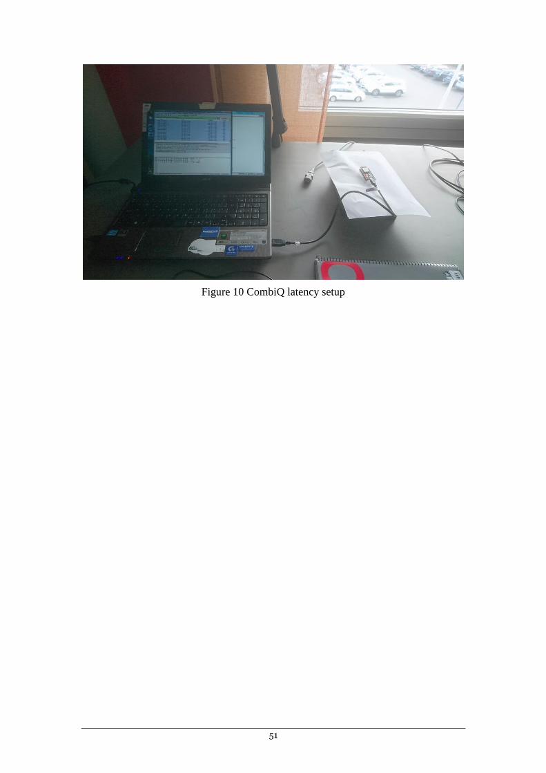
51

Figure 10 CombiQ latency setup

52

And for the power measurement setup, as seen in Figure 11.

Figure 11 CombiQ power setup

53

And the Wi-fi signals and signal strength as seen in Figure 12

Figure 12 CombiQ Wi-Fi Signals

The experiments at CombiQ were conducted in an environment where there were a lot of Wi-Fi networks. The Wi-Fi network used in the experiments are the upper red line seen in Figure 12, with a signal strength of -45 to -55 dBm.

While measuring the gateway to client latency using the ping command (where 50 messages with the size of 32 Bytes were sent). The results can be found in Table 6. However, it is worth mentioning that the high ping values were related to the stability of the network connection.

Min (ms) Avg (ms) Max (ms)

2 19 253

Table 6 CombiQ raw ping results

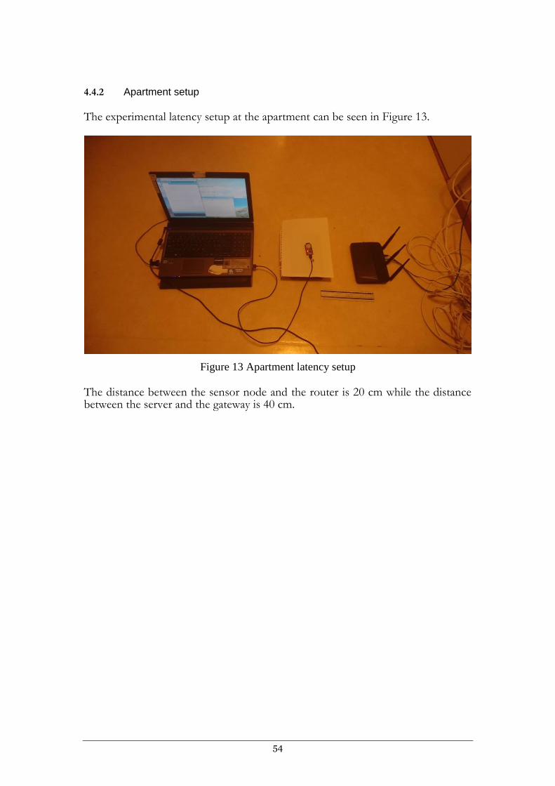
54

4.4.2 Apartment setup

The experimental latency setup at the apartment can be seen in Figure 13.

Figure 13 Apartment latency setup

The distance between the sensor node and the router is 20 cm while the distance between the server and the gateway is 40 cm.

55

Wi-Fi signals and signal strength as seen in Figure 14.

Figure 14 Apartment Wi-Fi signals

The experiments at apartment were conducted in an environment where there were a lot of Wi-Fi networks. The Wi-Fi network used in the experiments were the upper red line seen in Figure 14, with a signal strength of -30 to -40 dBm.

While measuring the gateway to client latency using the ping command (where 50 messages with the size of 32 Bytes were sent). The results of the ping command can be found in Table 7.

Min (ms) Avg (ms) Max (ms)

1 3 10

Table 7 Apartment raw ping results

56

5 Findings and analysis

This chapter will present the findings of the experiments as well as analysis of the collected data. The results will be shown in its own paragraph for each communication protocol as well as environment. The analysis of the findings will be described and the hypothesis will be tested.

5.1 Findings

In this section, the findings of all the experiments will be presented.

5.1.1 Latency findings

This section is dedicated to show the results of the latency measurements. The results presented here were processed and went through some data set reductions since some results contained anomalous data (i.e. data with a latency higher than 1000 ms) which impacted the calculated average significantly. This process is visualized in Figure 15.

The raw results from the latency experiments can be found in section 8.2 for the communication protocol, QoS level and the usage environment.

Figure 15 Data Flow Latency

57

5.1.1.1 Latency findings for CombiQ MQTT QoS 0

CombiQ MQTT QoS 0

Msg Size 4 Bytes 16 Bytes 48 Bytes 92 Bytes 120 Bytes

Min (ms) 14,8 16,0 8,5 6,5 5,7

Avg (ms) 30,9 27,5 14,9 22,7 24,8

Max (ms) 167,9 47,6 47,2 184,6 115,9

StD (ms) 26,2 8,1 7,9 24,4 17,1

Table 8 CombiQ MQTT QoS 0 Latency


CombiQ MQTT QoS 1


Min (ms) 1,1 2,3 5,7 10,2 12,9

Avg (ms) 152,9 151,7 144,4 154,8 159,2

Max (ms) 428,5 280,3 269,7 289,2 309,1

StD (ms) 88,6 73,2 74,5 77,9 72,8


58


CombiQ MQTT QoS 2


Min (ms) 17,0 19,0 27,2 29,3 43,0

Avg (ms) 142,5 151,1 163,8 159,5 157,5

Max (ms) 340,1 367,7 353,5 292,1 384,0

StD (ms) 84,3 85,2 79,5 77,1 76,6


5.1.1.4 Average MQTT latency for CombiQ

Average MQTT Latency for CombiQ (ms)

Message Size

QoS 4 Bytes 16 Bytes 48 Bytes 92 Bytes 120 Bytes

0 30,9 27,5 14,9 22,7 24,8

1 152,9 151,7 144,4 154,8 159,2

2 142,5 151,1 163,8 159,5 157,5

Table 11 Average MQTT latency for CombiQ

59

5.1.1.6 Latency findings for Apartment MQTT QoS 0

Apartment QoS 0


Min (ms) 3,1 4,3 7,7 12,3 15,1

Avg (ms) 6,1 6,5 10,7 19,3 28,9

Max (ms) 47,0 15,2 72,0 124,3 206,0

StD (ms) 7,5 2,6 9,0 22,7 34,7

Table 12 Apartment MQTT QoS 0 Latency


Apartment QoS 1


Min (ms) 3,0 4,1 7,7 15,7 17,7

Avg (ms) 129,4 121,9 141,9 149,2 141,5

Max (ms) 250,1 244,6 294,5 259,6 262,9

StD (ms) 69,5 68,4 76,1 72,5 73,0



Apartment QoS 2


Min (ms) 2,2 7,5 13,4 12,6 16,4

Avg (ms) 124,2 121,2 132,2 138,9 143,5

Max (ms) 241,5 239,9 354,4 257,1 255,1

StD (ms) 70,5 74,7 78,5 76,6 70,3


5.1.1.9 Average MQTT latency for apartment

Average MQTT Latency for Apartment (ms)

Message Size

QoS 4 Bytes 16 Bytes 48 Bytes 92 Bytes 120 Bytes

0 6,1 6,5 10,7 19,3 28,9

1 129,4 121,9 141,9 149,2 141,5

2 124,2 121,2 132,2 138,9 143,5

Table 15 Average MQTT Latency for apartment

60

5.1.1.10 Latency findings for CombiQ CoAP

CoAP Latency at CombiQ(ms)

Msg Size 4 Bytes 16 Bytes 32 Bytes

Min (ms) 2,1 1,9 2,1

Avg (ms) 33,2 12,5 39,7

Max (ms) 666,1 334,6 702,2

StD (ms) 111,6 47,3 124,6

Table 16 CombiQ CoAP Latency

5.1.1.11 Latency findings for Apartment CoAP

CoAP Latency at Apartment (ms)

Msg Size 4 Bytes 16 Bytes 32 Bytes

Min (ms) 3,1 3,4 3,6

Avg (ms) 19,5 13,8 27,1

Max (ms) 226,1 176,1 212,9

StD (ms) 43,7 24,6 50,8

Table 17 Apartment CoAP Latency

61

5.1.2 Power consumption findings

This section is dedicated to show the power consumption findings, where the results are shown as Watt on the graph. The overall data processing is visualized in Figure 16 but it is also explained in paragraph 4.3.6.3

Due to a problem with the data collection, only 10 ms (interval of 1 ms) was recorded for each communication protocol. This makes it impossible to draw any conclusions regarding the power consumption since calculating the power consumption requires the whole 1000 ms period. This will further be discussed in chapter 6. However, screen dumps of the current on the oscilloscope can be found in section 8.3.

Figure 16 Data flow power consumption

62

5.2 Analysis

This section is dedicated to the interpretation of the data shown in the findings chapter as well as the raw data found in section 8.2. The analysis will be conducted with respect to the hypotheses and will visualize the data to make it easier to understand. This section will interpret the latency results. Lastly, the results will be compared with the hypotheses.

The power consumption findings as well as hypothesis 2 and 4 (H2 and H4) will not be analysed due to the problems mentioned in sub-section 5.1.2. Therefore, hypothesis H2 and H4 are considered inconclusive due to the data being inadequate.

5.2.1 Latency analysis

The MQTT data will first be compared to each other and then site wise. CoAP on the other hand will be compared site wise as it did not have any varying QoS settings in our experiments.

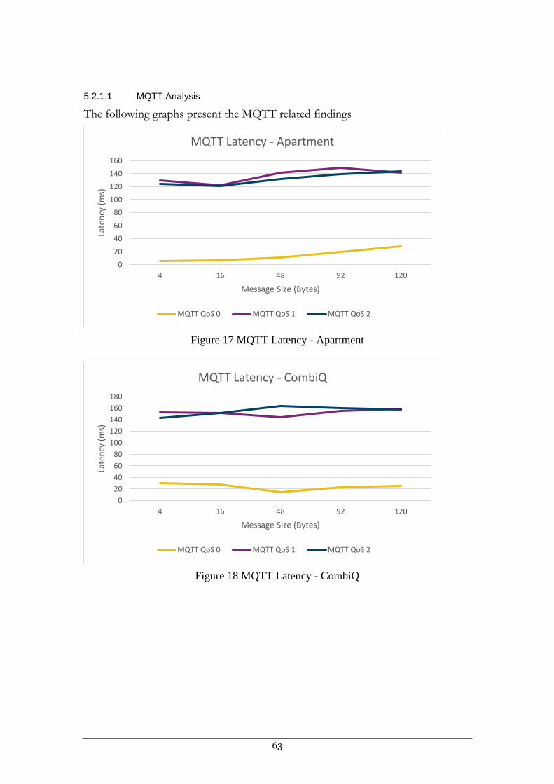
63

5.2.1.1 MQTT Analysis

The following graphs present the MQTT related findings

Figure 17 MQTT Latency - Apartment

Figure 18 MQTT Latency - CombiQ

0

20

40

60

80

100

120

140

160

4 16 48 92 120

Late

ncy

(m

s)


MQTT Latency - Apartment

MQTT QoS 0 MQTT QoS 1 MQTT QoS 2

0

20

40

60

80

100

120

140

160

180

4 16 48 92 120

Late

ncy

(m

s)


MQTT Latency - CombiQ

MQTT QoS 0 MQTT QoS 1 MQTT QoS 2

64

Figure 19 MQTT Latency - Both

The results for MQTT seems to suggest that the experiments done in the apartment have around 4 to 30 ms less latency on average than experiments carried out at CombiQ. However, this is only true for the higher QoS levels since the QoS level 0 experiment at the apartment for a message size of 120 Bytes had 4 ms higher latency than the same experiment carried out at CombiQ (see Figure 19)

As seen in the first two figures (See Figure 17, Figure 18), QoS level 1 and 2 did not seem to have a significant impact when compared to each other as they converged a lot. QoS level 0 on the other hand, had a much lower average latency than the higher QoS levels.

There was only one clear growth trend in these experiments, the apartment MQTT QoS 0 (Figure 17) experiments where the latency increased as the message size increased. However, compared to the other experiments done for MQTT, the results for this experiment could probably be coincidental since the other experiments shows a different growth pattern.

0

50

100

150

200

4 16 48 92 120

Late

ncy

(ms)


MQTT Latency - Both

MQTT QoS 0 A MQTT QoS 1 A MQTT QoS 2 A

MQTT QoS 0 C MQTT QoS 1 C MQTT QoS 2 C

65

5.2.1.2 CoAP Analysis

Figure 20 CoAP Latency - Both

The results for CoAP shows that the experiments done in the apartment have lower latency than the experiments at CombiQ. However, this is only true for message sizes 4 and 32 Bytes. The 16 Bytes message size experiment performed at CombiQ had a lower latency than the apartment counterpart.

It can also be stated that the growth trend is rather uncertain since it dips and rises. However, the experiments done at CombiQ seems to rise more sharply.

5.2.2 Hypothesis 1

The first hypothesis ” Using Higher QoS levels in MQTT should result in a higher latency since there are more messages sent before the message transaction is considered complete" is analyzed using the MQTT related findings as seen in Figure 17 ,Figure 18 and Figure 19.

While the results do not show that more message in the transaction equals longer latency, as seen in Figure 19, QoS level 1 and 2 have about the same latency (for the same site). The expected result was that QoS 2 should have higher latency than QoS 1 due to the additional messages, which would follow a similar pattern to Lindén’s [7] results. However, both MQTT with QoS level 0 and CoAP had much lower latency than MQTT QoS level 1 and 2 for both sites. Given this, the hypothesis (H1) cannot be considered supported by these experiments, due to the QoS level 1 and 2 latencies not being significantly different to each other (regardless of site). However, it can be said that the latency for MQTT is much lower when using QoS 0.

0

5

10

15

20

25

30

35

40

45

0 5 10 15 20 25 30 35

Late

ncy

(m

s)

Message Size(Bytes)

CoAP Latency Both

CoAP Apartment CoAP CombiQ

66

5.2.3 Hypothesis 3

The third hypothesis, “Using higher message sizes for a CoAP message transaction should result in higher latency, compared to if a lower message size were used”, is assessed with Figure 20, Table 16 and Table 17.

As seen in Figure 20, the latency for a 4 Bytes message is lower than the latency for a message of 32 Bytes for both sites. However, the results for message size 16 is much lower than message size 4 and 32 respectively, regardless of site. This mean that the hypothesis (H3) is not supported in this case.

5.2.4 Hypothesis 5

The fifth and last hypothesis, “Sensor nodes and gateways deployed in an usage environment where the signal strength is lower should have higher latency than usage environments with higher signal strength” , uses Figure 19 and Figure 20 to answer this hypothesis.

As described in the experiment preparation section 4.4, the CombiQ test environment corresponds to the usage environment with the lower signal strength (see Figure 12) and the apartment usage environment corresponds to the one with high signal strength (see Figure 14).

According to Figure 19, the latency results for the MQTT experiments done at the apartment almost certainly have a lower latency compared to the experiments performed at CombiQ. However, for MQTT QoS 0 the latency is a bit lower for a message size of 120 Bytes in CombiQ, this could be explained by anomalies in the data set or just by pure coincidence. Before making any assumptions, it would be wise to analyze the CoAP results to see if the data support or disprove this hypothesis.

The latency results for the CoAP experiments (Figure 20) show that the average latency is generally lower at the apartment compared to CombiQ. However, with the exception for the message size of 16 Bytes where CombiQ latency is just barely lower than the results gathered at the apartment.

Given the results, it can be said that MQTT’s and CoAP’s latency is generally lower in the apartment usage environment compared to the CombiQ usage environment. However, CoAP showed an inverted behavior where in CombiQ, the latency was generally lower than the latency measured in the apartment, for message size of 16 Bytes.

The hypothesis can be considered mostly supported when considering the MQTT results. However, according to the hypothesis description in paragraph 4.2.3.1, this hypothesis is not considered supported because of CoAP results.

67

6 Discussion and conclusions

The purpose of this chapter is to discuss the suitability of the general workflow, findings of the thesis and the conclusions drawn from the results and to look ahead and suggest future work. Firstly, a discussion whether the method and techniques used were suitable for the goal of the thesis will be held. After that the analyzed findings will be contrasted towards the research questions of the thesis. Lastly, the conclusions and future work will be described.

6.1 Discussion of method

6.1.1 Experimental research design

As mentioned in the research method chapter, this thesis used an experimental research design which was based on the experiment process described by Wohlin et al. [25]. The methods were used to validate hypotheses that describe how latency and power consumption is influenced by the usage environment as well as communication protocols.

The research method is suitable for the research purpose, as it gave the authors a lot of controllability when it came to the experiments. However, as mentioned by Wohlin et al. [25], the problems with the experiments are that they are time consuming, this was rather evident when planning and executing the experiments. This did lead to some rethinking regarding how the data should be collected, what the collected data would represent and how it would influence the overall goal of the thesis. In the end it can be said that the overall goal of this thesis remained the same.

This thesis did not fully answer its research questions. The power consumption and the data associated with was incomplete which made it impossible to clearly determine what the data is supposed to describe. This was at fault in the experiment planning and experiment execution as there were not enough time allocated to that aspect of the research. However, the applied experiment process (See Figure 6) could be more time efficient if the prototype experiments were conducted earlier in the process. Since it would double as a learning experience but also to discover what implementations can be used and how suitable they are. On the other hand, the latency data was complete and could be used in the analysis However, it did not yield any concrete answers to the latency related research questions because of poor reliability. This will be further discussed in sub-section 6.1.2

To conclude the discussion of the overall research design of this thesis, the authors think that the research design was suitable for the research goal. However, due to the time limitations there were parts in the thesis that did not get enough attention, which in the end, resulted in the first and second research question being partially answered. Furthermore, the research process could be improved by doing prototype experiments as early as possible in the process, and in parallel to other activities. This would allow the researcher to save time, since the researcher can explore and learn from the prototype experiments.

68

6.1.2 Validity and reliability of the research

This section is divided into 3 paragraphs that handle the internal and external validity as well as the reliability aspects of this thesis and the results within.

6.1.2.1 Internal validity

As mentioned in sub-section 4.3.7, this thesis used criterion based elimination of data set entries and increased data set size to make the analysis easier to perform.

These actions had a positive impact on the internal validity. The criterion based elimination did remove some outliers from the data set and the increased data set made it easier to see trends within the data. However, there is an inherent threat to the validity, which is related to the how the latency was measured, as mentioned in paragraph 4.3.4.4.

The latency measuring method used in this thesis cannot accurately determine the latency, since it uses a response message to calculate the time it takes for the message transaction to be considered complete. The main problem with this method is that it uses additional messages, which makes the latency results even more susceptible to propagation delays as well as signal strength variation. As mentioned earlier in paragraph 4.3.4.4, this could be solved if the time was synchronized between the sensor node and the gateway.

When it came to the usage environments, the authors did not have control over any eventual network instabilities that may have influenced the results. This caused the results to be less valid and reliable since it is not clear how much the network instabilities might have influenced the latency findings.

6.1.2.2 External validity

The design of this research can be applied to other communication protocols, sites and radio frequency transmitters. The analysis of the latency showed that the results themselves seemed to be similar. If the same experiment treatments were conducted at other sites that are alike it would have shown similar trends. However, it is important to mention that the experiments were not subjected to bandwidth limitations, which could influence latency.

6.1.2.3 Reliability

Given the results and the oscillation of the latency data (as seen in section 8.2) the results are not reliable. Additionally, if the sites are too different from the ones used in this thesis (for example if they have more interference) it would be unclear how the usage environment would influence the latency.

6.2 Discussion of findings

This section will contrast the analyzed findings and hypotheses with regards to the research questions.

69

6.2.1 RQ1

The first research question, ”How does MQTT impact latency and power consumption on a constrained device?”, have two related hypotheses (H1 and H2). This research question seeks to investigate how MQTT and its quality of service levels influence latency and power consumption.

Regarding the latency, the analysis and findings showed that MQTT with QoS level 0 had a much lower latency than MQTT with higher QoS levels (i.e. 1 and 2). The findings also showed, for the message sizes used, that the latency did not reliably increase as the message size increased, and instead seemed to not follow a pattern, except for MQTT QoS level 0 apartment experiment which showed a rising trend.

For the power consumption. The analysis could not be carried out because of an error with the data collection. The oscilloscope did only record the voltage for a 10 ms period which is not enough to draw any conclusions from. Since there is an uncertainty if oscilloscope managed to record whole message transaction during the 10 ms period. Especially when the latency results for QoS level 1 and 2 suggest that an average connection period (as well as latency) lasts around 140 to 160 ms (See Table 9 and Table 10).

To conclude this research question, the data suggest that MQTT’s QoS levels can influence the latency. However, the poor reliability of the data makes this unclear as the result could be influenced by an unknown factor. As for the power consumption, no conclusion could be made.

6.2.2 RQ2

The second research question, ”How does CoAP impact latency and power consumption on a constrained device?”, have two hypotheses related to it (H3 and H4). The goal of this research question is to investigate how CoAP influences the latency and power consumption.

For the latency, the analysis and findings showed that the latency for CoAP did not reliably increase as the message size increased, since there was a case (for both usage environments) where the latency was lower for a higher message size.

For the power consumption, hypothesis 4. The analysis could not be carried out and therefore no conclusions could be made about the power consumption.

Overall, no clear conclusions could be made from this research question and its findings.

6.2.3 RQ3

The third research question, ”How does usage environment influence the latency for MQTT and CoAP?”, have one hypothesis related to it (H5). The goal of this research question is to investigate how the usage environment influences MQTT and CoAP’s latency.

For MQTT, the data suggest that the usage environment has a small impact on the average latency, where the experiments performed at the apartment almost always

70

had lower latency than the experiments performed at CombiQ. However, there was one exception (MQTT with QoS level 0 for message size 120) where the CombiQ usage environment had lower latency than the MQTT usage environment.

For CoAP, like MQTT, the data suggested a small latency impact. The latency for CoAP was generally higher at CombiQ compared to the apartment. Additionally, there was one case (CoAP for message size of 16 Bytes) where the apartment latency was higher than the CombiQ latency.

This suggest that both MQTT and CoAP seems to perform better in the apartment usage environment (higher Wi-Fi signal strength).

6.3 Conclusions

So, to conclude this study, the results suggest that MQTT’s configuration can influence the latency at the cost of the quality of service. However, only between QoS 0 and 1 or QoS 0 and 2. The latency difference between QoS 1 and 2 did not have any obvious trends or behaviors at the given message sizes.

As for CoAP, its latency was seemingly unpredictable at the message sizes (i.e. up to 32 Bytes) used in this study. This made it harder to assess whether the latency would increase as the message size increased.

Lastly, the usage environment had a small impact on MQTT and CoAP latency, where usage environments with higher signal strength had lower latency than usage environments with lower signal strength.

Therefore, the configuration of the communication protocol as well as the usage environment where the device is deployed do influence the latency. However, it is not clear if there were any unknown factors influencing the results.

6.4 Future work

There are various areas of this work that could be improved and extended.

The power consumption aspect is one of them. The main problem with the power consumption is that the oscilloscope did not record the whole message transaction period. This could be fixed by using a different oscilloscope. A different path this could be carried out is to use a blue gecko card and simplicity studio to record the data. However, BLE, LoRaWAN or LTE-M would have to be used instead of Wi-Fi. After the data has been collected, the steps described in paragraph 4.3.6.3 and Figure 16 can be carried out and then the data can be analysed.

Additionally, if the power consumption data was correct. It would be hard to determine the cause and effect relationship between the code (or active task) and power increase. This would require some means of knowing whenever the code segment for the message transaction is executed. According to Joakim Gustafsson (See acknowledgements, page 3) from CombiQ, this can be achieved by using a digital probe together with an analogue probe, where the analogue probe is used to measure the overall power consumption and the digital probe is connected to a GPIO pin, which is activated whenever or before the publish/put command is executed and when the callback is executed. This method should produce a visible

71

line on the oscilloscope which shows when these commands are executed, which can help researchers identify the code and power relation.

Furthermore, this study can be extended (or repurposed) to utilize Bluetooth instead of Wi-Fi, for it to be more related to future trends within this area. As Bluetooth (specifically Bluetooth Low Energy) seem to have more interesting properties (in terms of power consumption). Additionally, different variables can be used such as distance between master and slave node which might impact other connectivity performance variables (such as error rate).

This thesis could be extended further by using a wider array of message sizes when doing the experiments. This may explain if the dips that occurred at 16 Bytes messages were caused by network instabilities.

Lastly, the latency related experiments could be performed at different sites to validate the claim that usage environments have impact on the connectivity performance or if the findings will be like the ones in this thesis.

72

7 References

[1] Ericsson, "Ericsson Mobility Report," June 2016. [Online]. Available: https://www.ericsson.com/res/docs/2016/ericsson-mobility-report-2016.pdf. [Accessed 3 April 2017].

[2] Cisco, "Cisco Visual Networking Index Predicts Near-Tripling of IP Traffic by 2020," Cisco, 7 June 2016. [Online]. Available: https://newsroom.cisco.com/press-release-content?type=press-release&articleId=1771211. [Accessed 21 November 2017].

[3] A. Flammini and E. Sisinni, “Wireless Sensor Networking in the Internet of Things and Cloud Computing Era,” in EUROSENSORS 2014, the XXVIII edition of the conference series, Brescia, 2014.

[4] M. F. Othman and K. Shazali, “Wireless Sensor Network Applications: A Study in Environment Monitoring System,” in International Symposium on Robotics and Intelligent Sensors 2012 (IRIS 2012), Engineering Procedia, 2012, pp. 1204-1210.

[5] OMA, "Constrained Application Protocol: CoAP Is IoT's 'Modern' Protocol," Open Mobile Alliance, 22 June 2016. [Online]. Available: http://openmobilealliance.org/in-the-news/constrained-application-protocol-coap-is-iots-modern-protocol. [Accessed 26 November 2017].

[6] M. B. Yassein, M. Q. Shatnawi and D. Al-zoubi, “Application layer protocols for the Internet of Things: A survey,” in International Conference on Engineering & MIS (ICEMIS), 2016.

[7] E. Lindén, “A latency comparison of IoT protocols in MES,” DiVA, 2017.

[8] D. Boyle, R. Kolcun and E. Yeatman, “Energy-Efficient Communication in Wireless Networks,” in ICT - Energy Concepts for Energy Efficiency and Sustainability, InTech, 2017.

[9] B. Jadhav, “Wireless technology - Wi-Fi,” 2013 May 2013. [Online]. Available: https://www.slideshare.net/mail2bhushan7/wireless-technology-wifi. [Accessed 23 November 2017].

[10] A. Banks and R. Gupta, “MQTT Version 3.1.1 Plus Errata 01,” 10 December 2015. [Online]. Available: http://docs.oasis-open.org/mqtt/mqtt/v3.1.1/errata01/os/mqtt-v3.1.1-errata01-os-complete.html. [Accessed 22 November 2017].

[11] "Frequently Asked Questions," [Online]. Available: http://mqtt.org/faq. [Accessed 19 April 2017].

[12] V. Lampkin, W. T. Leong, L. Olivera, S. Rawat, N. Subrahmanyam, R. Xiang, G. Kallas, N. Krishna, S. Fassman, M. Keen and D. Locke, Building Smarter Planet Solutions with MQTT and IBM WebSphere MQ Telemetry, IBM Redbooks, 2012.

[13] M. Kooijman, Building Wireless Sensor Networks Using Arduino, Packt Publishing, 2015.

[14] T. Jaffey, "MQTT and CoAP, IoT Protocols," February 2014. [Online]. Available: https://eclipse.org/community/eclipse_newsletter/2014/february/article2.php. [Accessed 19 April 2017].

[15] R. Webb, “A Brief, but Practical Introduction to the MQTT Protocol and its Application to IoT,” Zoetrope Limited, 23 Mars 2016. [Online]. Available: https://zoetrope.io/tech-blog/brief-practical-introduction-mqtt-protocol-and-its-application-iot. [Accessed 21 November 2017].

[16] C. Bormann and Z. Shelby, "Block-Wise Transfers in the Constrained Application Protocol (CoAP)," August 2016. [Online]. Available: https://www.rfc-editor.org/rfc/rfc7959.txt. [Accessed 19 April 2017].

[17] O. Tezer, “Digitalocean.com,” 23 December 2013. [Online]. Available: https://www.digitalocean.com/community/tutorials/an-advanced-message-queuing-protocol-amqp-walkthrough. [Accessed 21 November 2017].

[18] A. Piper, “Choosing Your Messaging Protocol: AMQP, MQTT, or STOMP,” VMware Inc., 19 February 2013. [Online]. Available:

73

https://blogs.vmware.com/vfabric/2013/02/choosing-your-messaging-protocol-amqp-mqtt-or-stomp.html. [Accessed 21 November 2017].

[19] Hacker News, “Clarifying AMQP | kellabyte,” 22 October 2012. [Online]. Available: https://www.tuicool.com/articles/fQnIni. [Accessed 2 December 2017].

[20] H. Subramoni, G. Marsh, S. Narravula, P. Lai and D. K. Panda, “Design and Evaluation of Benchmarks for Financial Applications using Advanced Message Queuing Protocol (AMQP) over InfiniBand,” Department of Computer Science and Engineering, The Ohio State University, 2008.

[21] P. Saint-Andre, "Extensible Messaging and Presence Protocol (XMPP): Core," March 2011. [Online]. Available: https://www.rfc-editor.org/rfc/rfc6120.txt. [Accessed 19 April 2017].

[22] "An Overview of XMPP," [Online]. Available: https://xmpp.org/about/technology-overview.html. [Accessed 19 April 2017].

[23] M. Müller, “Stack Exchange,” 29 May 2016. [Online]. Available: https://electronics.stackexchange.com/a/237027. [Accessed 10 April 2018].

[24] G. Z. Papadopoulos, K. Kritsis, A. Gallais, P. Chatzimisios and T. Noel, “Performance evaluation methods in ad hoc and wireless sensor networks: a literature study,” IEEE Communications Magazine, vol. 54, no. 1, pp. 122 - 128, 2016.

[25] C. Wohlin, P. Runeson, M. Höst, M. C. Ohlsson, B. Regnell and A. Wesslén, Experimentation in Software Engineering, Springer, 2012.

[26] J. Gähwiler, “Github,” 28 June 2017. [Online]. Available: https://github.com/256dpi/arduino-mqtt/blob/master/examples/ESP32DevelopmentBoard/ESP32DevelopmentBoard.ino. [Accessed 25 January 2018].

[27] H. Niisato, “Github,” 3 August 2017. [Online]. Available: https://github.com/hirotakaster/CoAP-simple-library/blob/master/examples/esp32/esp32.ino. [Accessed 25 January 2018].

74

8 Appendices

Appendice Content

8 Appendices .............................................................................. 74

8.1 CODE ..................................................................................................................................... 75

8.1.1 MQTT sensor node latency code .............................................................................. 75

8.1.2 MQTT sensor node energy code ............................................................................... 78

8.1.3 CoAP sensor node latency code ............................................................................... 80

8.1.4 CoAP sensor node energy code ............................................................................... 83

8.2 RAW DATA ............................................................................................................................. 85



8.2.3 Latency (ms) MQTT QoS level 2 CombiQ................................................................ 87


8.2.5 Latency (ms) MQTT QoS level 1 Apartment ........................................................... 89


8.2.7 Latency (ms) CoAP CombiQ ..................................................................................... 91

8.2.8 Latency (ms) CoAP Apartment ................................................................................ 92

8.3 OSCILLOSCOPE DATA ............................................................................................................. 93




8.3.4 Electrical potential findings for CoAP ..................................................................... 99

75

8.1 Code

8.1.1 MQTT sensor node latency code /* The MIT License (MIT) Copyright (c) 2015 Joël Gähwiler Permission is hereby granted, free of charge, to any person obtaining a copy of this software and associated documentation files (the "Software"), to deal in the Software without restriction, including without limitation the rights to use, copy, modify, merge, publish, distribute, sublicense, and/or sell copies of the Software, and to permit persons to whom the Software is furnished to do so, subject to the following conditions: The above copyright notice and this permission notice shall be included in all copies or substantial portions of the Software. THE SOFTWARE IS PROVIDED "AS IS", WITHOUT WARRANTY OF ANY KIND, EXPRESS OR IMPLIED, INCLUDING BUT NOT LIMITED TO THE WARRANTIES OF MERCHANTABILITY, FITNESS FOR A PARTICULAR PURPOSE AND NONINFRINGEMENT. IN NO EVENT SHALL THE AUTHORS OR COPYRIGHT HOLDERS BE LIABLE FOR ANY CLAIM, DAMAGES OR OTHER LIABILITY, WHETHER IN AN ACTION OF CONTRACT, TORT OR OTHERWISE, ARISING FROM, OUT OF OR IN CONNECTION WITH THE SOFTWARE OR THE USE OR OTHER DEALINGS IN THE SOFTWARE. */ /* * Originally based on Joël Gähwiler's ESP32 MQTT example * located here: https://github.com/256dpi/arduino-mqtt/blob/master/examples/ESP32DevelopmentBoard/ESP32DevelopmentBoard.ino * * Description of modifications: Repurposed the program to record how long time it takes * (in milli- and microseconds) for it to send a message till it gets a respones from the server. Also removed features that were not in use for the experiment. * Modifications/Additions By: Alexander Lagerqvist 2017-10-10 * */ #include <WiFi.h> #include <MQTTClient.h> const char ssid[] = "ssid"; const char pass[] = "password"; unsigned int TsB = 0; unsigned int TsE = 0; WiFiClient net; MQTTClient client; //Parameters for the networking part char* ipAddress = "xxx.xxx.xxx.xxx"; // Ip of the MQTT broker char* topic = "e"; // Name of the topic int qoslvl = 0; //Quality of service level, 0 - 2 int aMessages = 50; //how many messages will be sent. int i = 0; //counter //Payload settings

76

//Each payload is declared with +1 Byte, this is due to the null pointer that is included in each char array. This nullpointer is not sent in the message so ultimately the payload is still 4, 16 and etc. Bytes long. char payload[5] = "qwyx"; //char payload[17] = "qwyx,uiiosp,asdg"; //char payload[49] = "qwyx,uiiosp,asdg,gsgr,nrbb,wfkow,wfwwf,4232,3233"; //char payload[93] = "qwyx,uiiosp,asdg,gsgr,nrbb,wfkow,wfwwf,4232,3233,69gb,53f2,vkam2,jwen2,fj23h3,cn2i3,vleo2,12"; //char payload[121] = "qwyx,uiiosp,asdg,gsgr,nrbb,wfkow,wfwwf,4232,3233,69gb,3f2,vkam2,jwen2,fj23h3,cn2i3,vleo2,12fas,dfwff,vdsds,grwfwa,bfop"; unsigned long lastMillis = 0; void calcD(bool isVerbose) double DeltaTs = ((TsE - TsB) / 1000); double DeltaTs2 = DeltaTs / 2; if (isVerbose) Serial.print("TsE is: "); Serial.print(TsE); Serial.print("µs TsB is: "); Serial.print(TsB); Serial.print("µs Delta is: "); Serial.print(TsE - TsB); Serial.print("µs Exchange Latency is: "); Serial.print(DeltaTs); Serial.print(" ms Sending Latency is: "); Serial.print(DeltaTs2); Serial.print(" ms"); Serial.println(); else Serial.print(TsE); Serial.print(","); Serial.print(TsB); Serial.print(","); Serial.print(TsE - TsB); Serial.print(","); Serial.print(DeltaTs); Serial.print(","); Serial.print(DeltaTs2); Serial.println(); //Resets TsB and TsE so that the latency for the next package can be measured. TsB = 0; TsE = 0; void messageReceived(String &topic, String &payload) if (TsE == 0 && TsB != 0) TsE = micros(); calcD(false); else if (TsB != 0 && TsE != 0) calcD(false);

77

void setup() Serial.begin(115200); WiFi.begin(ssid, pass); Serial.println(strlen(payload)); client.begin(ipAddress, net); client.onMessage(messageReceived); connect(); void connect() Serial.print("checking wifi..."); while (WiFi.status() != WL_CONNECTED) Serial.print("."); delay(1000); Serial.print("\nconnecting..."); while (!client.connect("arduino", "try", "try")) Serial.print("."); delay(1000); Serial.println("\nconnected!"); client.subscribe(topic); void loop() client.loop(); if (!client.connected()) connect(); // publish a message roughly every second. if (millis() - lastMillis > 1000 && (i < aMessages)) lastMillis = millis(); //Checks if the Timestamp has any value if (TsB == 0) client.publish(topic, payload, false, qoslvl); TsB = micros(); i++;

78

8.1.2 MQTT sensor node energy code /* The MIT License (MIT) Copyright (c) 2015 Joël Gähwiler Permission is hereby granted, free of charge, to any person obtaining a copy of this software and associated documentation files (the "Software"), to deal in the Software without restriction, including without limitation the rights to use, copy, modify, merge, publish, distribute, sublicense, and/or sell copies of the Software, and to permit persons to whom the Software is furnished to do so, subject to the following conditions: The above copyright notice and this permission notice shall be included in all copies or substantial portions of the Software. THE SOFTWARE IS PROVIDED "AS IS", WITHOUT WARRANTY OF ANY KIND, EXPRESS OR IMPLIED, INCLUDING BUT NOT LIMITED TO THE WARRANTIES OF MERCHANTABILITY, FITNESS FOR A PARTICULAR PURPOSE AND NONINFRINGEMENT. IN NO EVENT SHALL THE AUTHORS OR COPYRIGHT HOLDERS BE LIABLE FOR ANY CLAIM, DAMAGES OR OTHER LIABILITY, WHETHER IN AN ACTION OF CONTRACT, TORT OR OTHERWISE, ARISING FROM, OUT OF OR IN CONNECTION WITH THE SOFTWARE OR THE USE OR OTHER DEALINGS IN THE SOFTWARE. */ /* * Originally based on Joël Gähwiler's ESP32 MQTT example * located here: https://github.com/256dpi/arduino-mqtt/blob/master/examples/ESP32DevelopmentBoard/ESP32DevelopmentBoard.ino * * Description of modifications: Repurposed the program to record how long time it takes * (in milli- and microseconds) for it to send a message till it gets a respones from the server. Also removed features that were not in use for the experiment. * Modifications/Additions By: Alexander Lagerqvist 2017-10-10 * */ #include <WiFi.h> #include <MQTTClient.h> const char ssid[] = "ss-id"; const char pass[] = "password"; WiFiClient net; MQTTClient client; //Parameters for the networking part char* ipAddress = "xxx.xxx.xx.xxx"; // Ip of the MQTT broker char* topic = "e"; // Name of the topic int qoslvl = 1; //Quality of service level, 0 - 2 //Payload settings //Each payload is declared with +1 Byte, this is due to the null pointer that is included in each char array. This nullpointer is not sent in the message so ultimately the payload is still 16 Bytes long. char payload[17] = "qwyx,uiiosp,asdg"; unsigned long lastMillis = 0;

79

void messageReceived(String &topic, String &payload) void setup() Serial.begin(115200); WiFi.begin(ssid, pass); Serial.println(strlen(payload)); client.begin(ipAddress, net); client.onMessage(messageReceived); connect(); void connect() Serial.print("checking wifi..."); while (WiFi.status() != WL_CONNECTED) Serial.print("."); delay(1000); Serial.print("\nconnecting..."); while (!client.connect("arduino", "try", "try")) Serial.print("."); delay(1000); Serial.println("\nconnected!"); client.subscribe(topic); void loop() client.loop(); if (!client.connected()) connect(); // publish a message roughly every second. if (millis() - lastMillis > 1000) lastMillis = millis(); //Checks if the Timestamp has any value client.publish(topic, payload, false, qoslvl);

80

8.1.3 CoAP sensor node latency code /* Copyright (c) 2018 Hirotaka Niisato This software is released under the MIT License. Permission is hereby granted, free of charge, to any person obtaining a copy of this software and associated documentation files (the "Software"), to deal in the Software without restriction, including without limitation the rights to use, copy, modify, merge, publish, distribute, sublicense, and/or sell copies of the Software, and to permit persons to whom the Software is furnished to do so, subject to the following conditions: The above copyright notice and this permission notice shall be included in all copies or substantial portions of the Software. THE SOFTWARE IS PROVIDED "AS IS", WITHOUT WARRANTY OF ANY KIND, EXPRESS OR IMPLIED, INCLUDING BUT NOT LIMITED TO THE WARRANTIES OF MERCHANTABILITY, FITNESS FOR A PARTICULAR PURPOSE AND NONINFRINGEMENT. IN NO EVENT SHALL THE AUTHORS OR COPYRIGHT HOLDERS BE LIABLE FOR ANY CLAIM, DAMAGES OR OTHER LIABILITY, WHETHER IN AN ACTION OF CONTRACT, TORT OR OTHERWISE, ARISING FROM, OUT OF OR IN CONNECTION WITH THE SOFTWARE OR THE USE OR OTHER DEALINGS IN THE SOFTWARE. */ /* * Originally based on Hirotaka's ESP32 CoAP example * located here: https://github.com/hirotakaster/CoAP-simple-library/blob/master/examples/esp32/esp32.ino * * Description of modifications: Repurposed the program to record how long time it takes * (in milli- and microseconds) for it to send a message till it gets a respones from the server. Also removed features that were not in use for the experiment. * Modifications/Additions By: Alexander Lagerqvist 2017-10-10 * */ #include <WiFi.h> #include <WiFiUdp.h> #include <coap.h> const char* ssid = "ssid"; const char* password = "password"; unsigned int TsB = 0; unsigned int TsE = 0; unsigned long lastMillis = 0; //Parameters for the PUT method IPAddress ipAddress = IPAddress(XXX, XXX, XXX, XXX); // Ip of the Californium/CoAP server int port = 5683; // the port char* uri = "e"; // Name of the resource identifier int aMessages = 50; //how many messages will be sent. int i = 0; //counter //Payload settings

81

//Each payload is declared with +1 Byte, this is due to the null pointer that is included in each char array. This nullpointer is not sent in the message so ultimately the payload is still 4, 16 and etc. Bytes long. char payload[5] = "qwyx"; //char payload[17] = "qwyx,uiiosp,asdg"; //char payload[35] = "qwyx,uiiosp,asdg,qwyx,uiiospde2gk1"; //char payload[49] = "qwyx,uiiosp,asdg,gsgr,nrbb,wfkow,wfwwf,4232,3233"; //char payload[93] = "qwyx,uiiosp,asdg,gsgr,nrbb,wfkow,wfwwf,4232,3233,69gb,53f2,vkam2,jwen2,fj23h3,cn2i3,vleo2,12"; //char payload[121] = "qwyx,uiiosp,asdg,gsgr,nrbb,wfkow,wfwwf,4232,3233,69gb,3f2,vkam2,jwen2,fj23h3,cn2i3,vleo2,12fas,dfwff,vdsds,grwfwa,bfop"; // CoAP client response callback void callback_response(CoapPacket &packet, IPAddress ip, int port); // UDP and CoAP class WiFiUDP udp; Coap coap(udp); // CoAP client response callback void callback_response(CoapPacket &packet, IPAddress ip, int port) if (TsE == 0 && TsB != 0) TsE = micros(); calcD(false); void calcD(bool isVerbose) float DeltaTs = ((TsE - TsB) / 1000); float DeltaTs2 = DeltaTs / 2; if (isVerbose) Serial.print("TsE is: "); Serial.print(TsE); Serial.print("µs TsB is: "); Serial.print(TsB); Serial.print("µs Delta is: "); Serial.print(TsE - TsB); Serial.print("µs Exchange Latency is: "); Serial.print(DeltaTs); Serial.print(" ms Sending Latency is: "); Serial.print(DeltaTs2); Serial.print(" ms"); Serial.println(); else Serial.print(TsE); Serial.print(","); Serial.print(TsB); Serial.print(","); Serial.print(TsE - TsB); Serial.print(","); Serial.print(DeltaTs); Serial.print(","); Serial.print(DeltaTs2); Serial.println();

82

//Resets TsB and TsE so that the latency for the next package can be measured. TsB = 0; TsE = 0; void setup() Serial.begin(115200); Serial.println(strlen(payload)); WiFi.begin(ssid, password); while (WiFi.status() != WL_CONNECTED) delay(500); Serial.print("."); Serial.println(""); Serial.println("WiFi connected"); Serial.println("IP address: "); Serial.println(WiFi.localIP()); //sets the response callback and starts the coap server/client coap.response(callback_response); coap.start(); void loop() coap.loop(); if (millis() - lastMillis > 1000 && (i < aMessages)) lastMillis = millis(); //Checks if the Timestamp has any value if (TsB == 0) coap.put(ipAddress, port, uri, payload); TsB = micros(); i++;

83

8.1.4 CoAP sensor node energy code /* Copyright (c) 2018 Hirotaka Niisato This software is released under the MIT License. Permission is hereby granted, free of charge, to any person obtaining a copy of this software and associated documentation files (the "Software"), to deal in the Software without restriction, including without limitation the rights to use, copy, modify, merge, publish, distribute, sublicense, and/or sell copies of the Software, and to permit persons to whom the Software is furnished to do so, subject to the following conditions: The above copyright notice and this permission notice shall be included in all copies or substantial portions of the Software. THE SOFTWARE IS PROVIDED "AS IS", WITHOUT WARRANTY OF ANY KIND, EXPRESS OR IMPLIED, INCLUDING BUT NOT LIMITED TO THE WARRANTIES OF MERCHANTABILITY, FITNESS FOR A PARTICULAR PURPOSE AND NONINFRINGEMENT. IN NO EVENT SHALL THE AUTHORS OR COPYRIGHT HOLDERS BE LIABLE FOR ANY CLAIM, DAMAGES OR OTHER LIABILITY, WHETHER IN AN ACTION OF CONTRACT, TORT OR OTHERWISE, ARISING FROM, OUT OF OR IN CONNECTION WITH THE SOFTWARE OR THE USE OR OTHER DEALINGS IN THE SOFTWARE. */ /* * Originally based on Hirotaka's ESP32 CoAP example * located here: https://github.com/hirotakaster/CoAP-simple-library/blob/master/examples/esp32/esp32.ino * * Description of modifications: Repurposed the program to record how long time it takes * (in milli- and microseconds) for it to send a message till it gets a respones from the server. Also removed features that were not in use for the experiment. * Modifications/Additions By: Alexander Lagerqvist 2017-10-10 * */ #include <WiFi.h> #include <WiFiUdp.h> #include <coap.h> const char* ssid = "ss-id"; const char* password = "password"; unsigned long lastMillis = 0; //Parameters for the PUT method IPAddress ipAddress = IPAddress(xxx, xxx, xx, xxx); // Ip of the Californium/CoAP server int port = 5683; // the port char* uri = "e"; // Name of the resource identifier //Payload settings //Each payload is declared with +1 Byte, this is due to the null pointer that is included in each char array. This nullpointer is not sent in the message so ultimately the payload is still 16 Bytes long. char payload[17] = "qwyx,uiiosp,asdg"; // CoAP client response callback void callback_response(CoapPacket &packet, IPAddress ip, int port);

84

// UDP and CoAP class WiFiUDP udp; Coap coap(udp); // CoAP client response callback void callback_response(CoapPacket &packet, IPAddress ip, int port) void setup() Serial.begin(115200); Serial.println(strlen(payload)); WiFi.begin(ssid, password); while (WiFi.status() != WL_CONNECTED) delay(500); Serial.print("."); Serial.println(""); Serial.println("WiFi connected"); Serial.println("IP address: "); Serial.println(WiFi.localIP()); //sets the response callback and starts the coap server/client coap.response(callback_response); coap.start(); void loop() coap.loop(); if (millis() - lastMillis > 1000) lastMillis = millis(); //Checks if the Timestamp has any value coap.put(ipAddress, port, uri, payload);

85

8.2 Raw data

8.2.1 Latency (ms) MQTT QoS level 0 CombiQ Message Size 4

Message Size 16

Message Size 48

Message Size 92

Message Size 120

20,967 39,21 10,52 6,472 5,725 22,309 22,07 19,428 16,821 19,298 18,623 19,677 47,195 14,605 18,937 17,681 29,95 9,51 16,118 17,77 19,649 31,73 9,485 15,853 20,677 32,837 18,375 20,864 26,048 28,289 31,619 15,952 10,323 22,423 26,743 23,975 37,178 8,486 17,994 18,214 52,277 40,463 16,061 14,532 20,297 30,845 38,27 9,597 22,078 17,671 46,499 25,086 22,281 25,022 22,265 20,057 45,274 10,246 19,865 17,298 36,325 24,955 15,347 17,142 17,199 56,592 22,832 15,398 17,529 19,809 20,295 19,135 10,235 13,783 29,022 16,461 18,55 11,324 22,84 33,252 24,371 18,356 10,183 19,47 23,596

128,326 26,581 16,48 17,549 15,86 25,367 37,143 14,814 19,529 21,127

167,949 23,067 8,789 28,633 19,873 19,953 23,223 12,171 21,733 81,982 29,467 24,947 9,037 17,385 17,229 17,643 1174,466 1196,926 14,606 115,919 24,733 19,593 11,394 17,111 18,497 16,867 2151,855 12,355 17,869 1468,793 14,808 24,992 9,503 17,207 15,95 23,597 1574,287 1532,414 17,019 22,62

1378,857 35,816 9,206 22,027 4027,604 27,905 30,814 11,566 18,044 23,143 19,395 29,984 36,077 17,157 19,924 19,383 24,142 18,341 14,95 17,209 21,421 29,569 9,681 14,233 22,756

23,204 32,507 9,928 18,035 20,348 21,672 25,698 34,095 40,623 22,166 26,218 41,518 22,712 20,949 26,103 29,406 27,667 21,98 13,965 22,588 27,488 30,137 9,927 28,186 19,225 24,854 47,633 11,808 14,852 21,765 42,132 21,132 14,759 14,993 21,103 21,709 19,197 13,161 1545,194 22,291 32,395 25,227 15,897 43,054 25,601 18,481 16,852 9,85 184,564 36,269

17,68 17,022 12,611 20,196 22,219 25,784 24,873 11,694 13,759 16,384 26,576 24,097 12,461 21,345 28,231 29,571 41,088 8,733 27,455 17,153

26,069 24,996 13,208 15,046 46,798 23,243 20,889 20,288 14,137 16,446 23,802 21,637 29,24 16,748 17,928 26,189 34,673 8,908 23,05 19,877

Table 18 Raw MQTT QoS 0 CombiQ Latency

86

8.2.2 Latency (ms) MQTT QoS level 1 CombiQ

Message Size 4

Message Size 16

Message Size 48

Message Size 92

Message Size 120

1,075 2,308 5,669 10,243 12,944

67,068 209,918 56,325 224,09 233,756

57,337 189,084 241,885 156,311 114,103

30,59 164,261 194,339 63,149 257,838

23,783 155,068 148,454 201,583 138,993

257,839 131,681 100,559 121,018 309,098

243,161 122,054 269,708 267,139 155,616

227,722 76,247 240,942 185,055 35,922

213,673 68,391 186,787 101,354 186,539

219,141 38,973 132,399 253,953 69,388

204,054 259,325 88,807 151,404 194,562

200,746 233,274 28,515 76,851 82,297

189,782 230,085 239,813 256,466 227,032

164,206 193,562 188,894 133,152 109,834

166,085 158,922 144,751 30,339 239,886

153,788 152,877 92,48 224,859 131,613

132,377 129,375 255,084 125,96 261,655

428,535 117,942 239,915 23,621 168,357

115,531 88,121 175,485 183,511 46,664

89,895 54,05 112,942 88,571 191,452

96,908 30,831 60,48 263,706 60,962

67,496 247,758 255,028 168,943 217,919

105,819 228,503 207,755 56,867 97,806

55,319 210,736 171,003 234,474 219,593

53,379 197,013 128,025 133,814 91,281

20,107 164,856 62,142 49,581 251,166

264,809 151,539 265,792 207,388 136,682

241,709 123,553 202,352 98,898 241,539

232,75 81,209 157,423 266,641 153,158

222,253 29,023 111,196 184,788 34,646

213,504 46,494 43,21 97,802 188,727

202,325 280,339 248,772 257,519 93,136

180,503 242,161 87,707 168,969 202,229

191,741 225,988 109,816 269,745 91,078

164,749 213,336 24,07 218,885 219,733

149,679 181,828 50,666 123,106 109,463

166,413 162,359 120,96 39,599 253,821

130,141 141,561 157,223 193,768 125,693

121,401 90,421 140,698 105,971 213,765

122,64 81,05 103,793 289,181 161,229

109,027 61,327 45,903 186,598 44,384

81,551 41,397 240,537 79,157 191,275

107,445 266,725 187,189 242,854 204,169

59,5 254,759 139,671 154,86 196,023

48,663 235,023 85,429 58,914 100,562

268,54 190,13 35,273 212,499 210,242

20,34 201,127 228,764 129,876 95,221

332,502 154,536 188,396 33,908 211,256

208,42 147,848 131,899 212,401 121,307

219,827 123,922 86,733 122,149 256,205


87

8.2.3 Latency (ms) MQTT QoS level 2 CombiQ Message Size 4

Message Size 16

Message Size 48

Message Size 92

Message Size 120

234,732 220,267 221,54 229,115 244,362

86,475 46,54 166,343 254,351 75,851

65,608 31,328 105,405 174,375 193,39

238,289 265,207 264,411 91,495 67,924

51,947 211,441 251,227 231,615 200,459

272,998 193,985 200,034 140,949 79,165

238,26 162,961 135,631 39,473 233,393

207,394 157,222 82,074 212,367 91,836

221,857 99,968 264,642 95,718 242,959

205,796 87,136 231,014 278,024 102,394

151,903 74,647 176,484 170,473 238,356

103,433 36,724 108,012 77,339 132,345

80,385 296,35 33,759 240,778 249,55

65,938 233,081 256,825 146,326 129,114

38,569 221,275 185,273 29,33 253,172

340,137 174,493 141,318 181,886 137,214

89,873 166,626 70,808 102,014 275,828

66,453 117,764 251,914 251,945 146,163

18,512 102,165 230,255 159,083 269,541

16,971 68,825 167,689 65,798 178,01

18,426 39,179 122,047 216,425 53,044

259,036 254,855 54,788 121,513 177,058

253,532 240,793 252,988 285,522 47,342

213,228 222,275 198,721 180,798 174,7

207,232 173,794 132,409 60,368 66,528

176,537 172,824 47,487 240,313 203,646

174,164 139,757 290,307 153,976 86,847

156,042 122,631 240,185 46,039 209,808

146,157 100,285 155,447 181,071 93,705

93,266 82,515 112,046 127,247 211,991

100,76 45,452 65,227 292,118 104,447

36,841 367,706 252,577 166,023 126,22

66,443 323,658 193,343 74,921 113,289

63,942 205,038 128,804 70,939 383,956

45,373 184,624 94,658 86,009 54,015

258,117 275,4 27,17 72,529 207,355

273,814 105,446 226,174 221,522 161,145

230,725 82,279 159,868 257,143 264,62

208,068 76,648 102,918 252,586 172,434

196,121 54,974 44,37 240,659 42,954

179,343 18,995 232,715 58,358 182,557

199,799 252,727 183,405 218,992 54,552

174,287 245,017 116,076 132,652 158,034

133,556 181,59 69,517 49,961 70,726

120,682 159,509 260,508 201,154 198,701

103,544 140,578 227,722 101,858 76,71

71,561 110,73 155,77 252,218 212,876

39,564 113,299 108,463 158,992 119,835

90,468 52,831 38,555 60,243 209,841

41,228 39,243 353,457 221,776 94,619


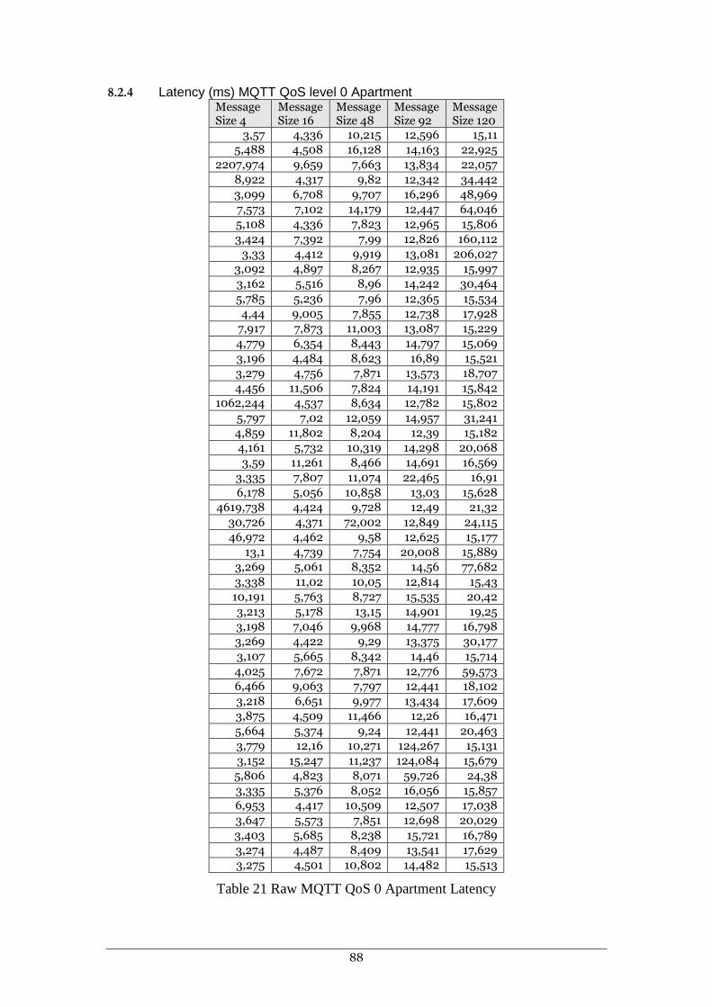
88

8.2.4 Latency (ms) MQTT QoS level 0 Apartment Message Size 4

Message Size 16

Message Size 48

Message Size 92

Message Size 120

3,57 4,336 10,215 12,596 15,11

5,488 4,508 16,128 14,163 22,925

2207,974 9,659 7,663 13,834 22,057

8,922 4,317 9,82 12,342 34,442

3,099 6,708 9,707 16,296 48,969

7,573 7,102 14,179 12,447 64,046

5,108 4,336 7,823 12,965 15,806

3,424 7,392 7,99 12,826 160,112

3,33 4,412 9,919 13,081 206,027

3,092 4,897 8,267 12,935 15,997

3,162 5,516 8,96 14,242 30,464

5,785 5,236 7,96 12,365 15,534

4,44 9,005 7,855 12,738 17,928

7,917 7,873 11,003 13,087 15,229

4,779 6,354 8,443 14,797 15,069

3,196 4,484 8,623 16,89 15,521

3,279 4,756 7,871 13,573 18,707

4,456 11,506 7,824 14,191 15,842

1062,244 4,537 8,634 12,782 15,802

5,797 7,02 12,059 14,957 31,241

4,859 11,802 8,204 12,39 15,182

4,161 5,732 10,319 14,298 20,068

3,59 11,261 8,466 14,691 16,569

3,335 7,807 11,074 22,465 16,91

6,178 5,056 10,858 13,03 15,628

4619,738 4,424 9,728 12,49 21,32

30,726 4,371 72,002 12,849 24,115

46,972 4,462 9,58 12,625 15,177

13,1 4,739 7,754 20,008 15,889

3,269 5,061 8,352 14,56 77,682

3,338 11,02 10,05 12,814 15,43

10,191 5,763 8,727 15,535 20,42

3,213 5,178 13,15 14,901 19,25

3,198 7,046 9,968 14,777 16,798

3,269 4,422 9,29 13,375 30,177

3,107 5,665 8,342 14,46 15,714

4,025 7,672 7,871 12,776 59,573

6,466 9,063 7,797 12,441 18,102

3,218 6,651 9,977 13,434 17,609

3,875 4,509 11,466 12,26 16,471

5,664 5,374 9,24 12,441 20,463

3,779 12,16 10,271 124,267 15,131

3,152 15,247 11,237 124,084 15,679

5,806 4,823 8,071 59,726 24,38

3,335 5,376 8,052 16,056 15,857

6,953 4,417 10,509 12,507 17,038

3,647 5,573 7,851 12,698 20,029

3,403 5,685 8,238 15,721 16,789

3,274 4,487 8,409 13,541 17,629

3,275 4,501 10,802 14,482 15,513

Table 21 Raw MQTT QoS 0 Apartment Latency

89


Message Size 16

Message Size 48

Message Size 92

Message Size 120

192,357 208,945 206,426 166,102 56,569

178,547 187,043 157,951 75,09 193,535

176,084 165,325 109,046 233,912 80,842

158,537 147,733 160,879 152,668 219,051

145,747 121,67 7,743 53,246 100,292

87,649 102,487 210,647 214,936 235,773

169,533 80,378 152,078 129,151 123,366

86,061 53,452 107,316 30,774 262,926

102,434 31,727 51,728 195,435 145,975

93,744 4,08 252,258 102,348 31,696

92,548 232,48 195,996 259,61 170,013

62,556 211,976 149,582 167,028 55,784

62,789 189,153 97,265 75,613 191,271

55,79 166,992 294,506 239,72 78,517

35,717 143,229 244,947 145,536 216,497

25,921 124,471 197,418 53,251 98,221

16,681 93,002 145,826 213,465 183,494

3,003 78,395 89,046 121,83 120,671

238,461 54,554 40,108 36,034 254,075

243,386 31,717 222,271 190,473 143,559

212,091 4,852 180,627 101,475 28,783

206,453 112,859 131,205 258,279 164,012

193,443 58,519 82,289 174,677 53,44

182,806 197,586 22,865 76,002 190,767

172,018 166,131 227,048 240,698 74,101

160,114 98,255 17,78 152,109 211,555

146,387 121,669 121,867 53,664 91,954

132,946 100,56 74,914 249,077 227,572

119,022 79,015 21,651 132,782 115,684

111,596 52,92 213,103 39,128 257,605

97,216 35,552 170,888 196,822 140,451

84,563 10,402 119,397 108,436 30,74

71,3 238,017 68,11 15,661 153,323

58,31 219,407 18,076 172,26 48,845

47,076 195,462 217,714 84,584 182,979

35,081 174,95 163,92 244,272 72,615

24,746 149,301 114,557 152,617 210,638

7,358 137,54 60,044 62,196 90,113

250,102 110,354 255,513 214,307 226,375

240,816 81,77 209,735 131,337 110,864

223,409 62,914 160,497 247,724 248,44

211,567 33,709 103,798 197,101 128,226

200,915 15,105 46,403 111,814 17,736

187,75 244,569 256,273 232,487 234,329

172,735 218,037 199,13 185,499 42,82

160,956 200,745 150,977 88,433 179,774

152,256 165,822 95,424 123,08 59,206

136,823 149,056 51,959 255,077 204,696

129,118 125,804 248,792 71,33 90,07

115,195 104,878 198,274 231,816 224,6


90


Message Size 16

Message Size 48

Message Size 92

Message Size 120

153,723 150,914 201,818 61,541 186,146

126,671 113,898 153,393 214,99 65,964

111,671 83,908 103,28 121,587 202,121

99,846 60,536 42,847 26,992 80,156

87,173 27,915 231,336 181,08 214,742

70,711 7,459 172,522 83,803 108,551

50,239 226,811 127,692 246,005 228,865

39,403 211,477 69,805 149,282 96,252

14,339 172,456 16,269 49,29 245,714

2,207 155,507 207,1 219,109 123,458

234,382 114,443 153,347 110,291 255,066

223,316 98,434 96,834 257,139 144,569

209,691 236,485 42,62 171,506 16,435

192,423 38,941 236,448 77,549 147,864

174,247 22,924 177,995 240,11 30,432

168,822 219,66 128,201 129,584 162,249

119,126 214,352 69,026 36,337 53,763

129,43 47,287 16,286 197,264 175,697

116,988 167,006 215,251 95,934 58,583

100,627 138,424 155,919 256,646 192,854

86,171 111,971 97,059 162,465 67,503

68,475 96,673 42,632 70,759 203,151

56,374 60,952 242,533 230,755 80,652

31,823 35,417 185,952 160,757 216,221

20,818 12,5 128,91 35,499 95,357

4,551 231,541 60,253 190,381 226,214

233,206 204,527 17,598 96,83 111,005

217,505 185,661 216,16 249,884 140,005

207,382 152,987 156,783 57,352 246,161

188,053 132,783 101,592 56,334 104,43

167,55 103,442 44,756 217,055 237,712

159,501 26,234 234,225 121,093 20,397

132,705 48,29 191,468 24,819 146,101

126,071 18,304 126,154 181,523 32,118

104,416 239,856 77,07 90,408 173,44

85,814 213,097 18,752 244,645 53,245

77,376 193,222 206,71 143,624 176,972

62,345 162,614 163,666 51,936 65,119

47,144 132,629 100,727 211,286 198,119

31,478 106,643 46,35 106,417 77,906

12,217 81,461 354,374 21,644 213,865

241,543 47,979 173,582 172,248 92,391

232,187 29,791 39,706 69,92 228,955

217,18 9,573 171,034 236,476 110,838

198,099 229 13,392 141,591 242,694

182,6 203,167 217,14 40,87 118,976

172,63 179,461 161,842 195,559 252,259

153,995 149,805 85,736 202,676 140,708

140,595 140,921 69,404 12,619 153,552

126,859 9,148 246,553 223,252 157,548


91

8.2.7 Latency (ms) CoAP CombiQ Message Size 4

Message Size 16

Message Size 32

666,116 1184,56 162,325

3,949 7,462 5,115

5,205 2,634 2,684

2,47 334,599 3,802

9,764 40,773 2,189

4,269 2,444 702,216

102,876 2,325 31,258

10,087 6,047 2,073

3,246 4,924 9,164

395,825 2,125 4,213

23,366 4,195 212,654

2,656 7,609 5,098

3,842 2,443 2,302

2,738 3,834 5,399

7,49 2,415 8,154

4,343 2,448 3,588

2,485 14,404 3,941

3,44 5,493 4,255

6,383 4,203 6,9

3,886 3,707 3,38

4,115 2,195 5,89

4,375 2,54 6,776

2,324 5,598 9,205

11,965 2,09 11,629

5,329 2,171 6,027

2,641 6,675 2,54

4,877 4,934 108,549

2,055 2,661 9,991

6,465 5,276 5,598

2,385 1,887 8,561

11,001 5,16 3,237

7,087 9,543 5,648

2,178 3,983 2,888

2,48 5,025 5,469

4,26 5,235 5,717

5,686 3,138 4,016

14,633 2,263 2,112

3,6 8,069 509,592

2,5 15,859 4,103

40,365 3,586 39,834

226,818 2,962 8,302

6,189 5,246 2,561

2,142 7,538 2,6

2,935 2,984 2,607

3,434 8,649 8,313

2,211 5,002 5,113

2,816 10,421 4,491

3,539 4,41 4,573

3,004 12,571 4,249

2,126 2,86 3,726

Table 24 Raw CoAP CombiQ Latency

92

8.2.8 Latency (ms) CoAP Apartment Message Size 4

Message Size 16

Message Size 32

215,73 176,104 192,099

5,745 4,534 9,905

4,611 4,462 5,757

5,868 8,975 7,19

7,708 4,266 5,773

17,247 19,75 12,096

4,588 5,487 6,736

10,445 4,381 13,095

3,763 8,932 12,405

11,731 14,989 12,571

3,286 19,468 7,583

7,566 3,491 9,847

12,583 10,968 5,968

5,667 4,217 3,562

11,815 7,301 4,666

6,616 7,431 19,639

8,599 3,544 15,905

5,535 22,748 5,221

15,221 13,867 7,917

4,449 31,901 10,422

4,097 8,261 8,508

15,637 8,709 9,819

3,55 3,468 10,552

7,497 6,816 6,082

5,462 6,415 11,977

10,765 5,766 212,916

4,979 23,645 132,275

23,248 11,738 167,673

5,638 17,596 90,091

3,773 4,048 10,769

21,549 9,215 150,382

21,415 6,771 6,414

16,574 22,362 6,097

3,491 7,678 11,498

226,083 23,48 6,439

5,843 4,674 5,756

14,992 35,219 26,605

92,16 3,382 7,874

5,798 4,766 15,471

39,668 12,631 9,743

9,604 7,116 4,28

10,632 20,997 5,702

4,5 5,545 3,83

12,901 10,056 8,574

4,058 5,323 5,453

9,752 9,08 6,603

3,091 4,649 8,828

3,893 5,198 20,428

3,456 8,473 6,522

10,569 10,81 8,776

Table 25 Raw CoAP Apartment Latency

93

8.3 Oscilloscope data

8.3.1 Electrical potential findings for MQTT QoS 0

Figure 21 MQTT QoS 0 1.000 ms

94

Figure 22 MQTT QoS 0, 500.0 ms

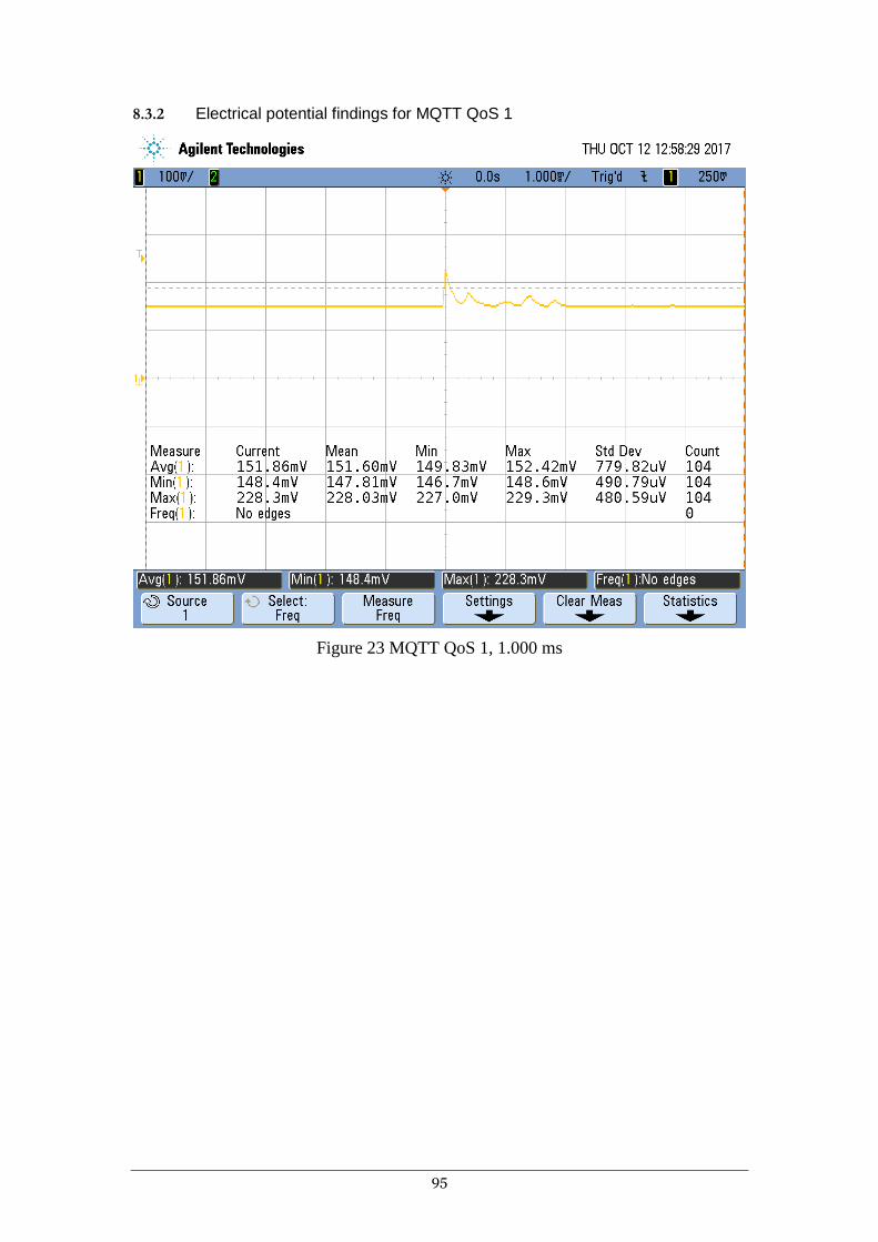
95



96


97



98


99

8.3.4 Electrical potential findings for CoAP

Figure 27 CoAP, 1.000 ms

100

Figure 28 CoAP, 500.0 ms

iot latency and power consumption -...

Documents