Ionization of Model Atomic Systems by

Periodic Forcings of Arbitrary Size

Joel L. Lebowitz

Departments of Mathematics and Physics

Rutgers University

(Joint work with O. Costin, R. Costin, A. Rokhlenko, C. Stucchio

and S. Tanveer)

1

Setting

We study the long time behavior of the solution of the Schrodinger

equation in d dimensions (in units such that ~ = 2m = 1),

i∂tψ(x, t) = [−∆ + V0(x) + V1(x, t)]ψ(x, t) (1)

Here, x ∈ Rd, t ≥ 0, V0(x) is a binding potential such

that H0 = −∆ + V0 has both bound and continuum states, and

V1(x, t) =∞∑

j=1

[

Ωj(x)eijωt + c.c

]

(2)

is a time-periodic potential. The initial condition, ψ(x,0) = ψ0(x) is

taken to be in L2(Rd).

2

Ionization

Our primary interest is whether the system ionizes under the in-

fluence of the forcing V1(x, t), as well as the rate of ionization if it

occurs. Ionization corresponds to delocalization of the wavefunction

as t → ∞. We say that the system, e.g. a Hydrogen atom, (fully)

ionizes if the probability of finding the electron in any bounded spa-

tial region B ⊂ Rd goes to zero as time becomes large, i.e.

P(BR, t) =

∫

|x|<R|ψ(x, t)|2dx→ 0, (3)

as t→ ∞.

3

The Floquet Connection

A simple way in which ionization may fail is the existence of a solution

of the Schrodinger equation in the form

ψ(t, x) = eiφtv(t, x) (4)

with φ ∈ R and υ ∈ L2([0,2π/ω] × Rd) time periodic. This leads to

the equation:

Kυ = φυ (5)

where

K = i∂

∂t− (−∆ + V0(x) + V1(x, t)) (6)

is the Floquet operator.(5) with 0 6= υ ∈ L2 means by definition,

that φ ∈ σd(K), the discrete spectrum of K.

4

Somewhat surprisingly, in all systems we studied σd(K) 6= ∅ is in fact

the only possibility for ionization to fail.

A proof of ionization then implies that K does not have any point, or

singular continuous, spectrum. This turns out to be a consequence

of the existence of an underlying compact operator formulation, the

operator being closely related to K.

Ionization is then expected generically since L2 solutions of the

Schrodinger equation of the special form (eiφtv) are unlikely. One

can also use phase space (entropy) arguments in favor of generic ion-

ization. Once the particle manages to escape into the “big world”

it will never return as is true for random perturbations (Pillet). Still,

mathematical physicists want proofs. We provide such proofs for

certain classes of systems and also find some nongeneric counterex-

amples.

5

Laplace space formulation

The propagator U(t, x) which solves the Schrodinger equation is

unitary and strongly differentiable in t. This implies that for

ψ0 ∈ L2(Rd), the Laplace transform

ψ(p, ·) :=∫ ∞

0ψ(t, ·)e−ptdt (7)

exists for p ∈ H, the right half complex plane, and the map p→ ψ is

L2 valued analytic for Re p > 0.

The Laplace transform converts the asymptotic problem (3) into an

analytical one involving the structure of singularities of ψ(p, x) for

Re p ≤ 0. In particular, ionization will occur if ψ(p, ·) has no poles

on the imaginary axis when V1 6= 0.

6

When V1 = 0 there will be poles of ψ at p = −iEn, En the eigenvalues

of the bound states of H0. As V1 is turned on these poles are

expected to move into the left complex plane, forming resonances.

This has in fact been proven rigorously for small enough

V1 = Ex cosωt when V0 is a dilation analytic potential, by various

authors.

In particular Sandro Graffi and Kenji Yajima proved this in 1983

for the Coloumb potential, V0 = −b/|x|, x ∈ R3.

This does not imply, however the absence of poles (resonances)

on the imaginary axis for finite strength V1. We rule this out in

the cases treated by using the Fredholm alternative on a suitable

compact operator. We also find some non-generic examples where

ionization fails.

7

Simple calculations show that ψ satisfies the equation

(H0 − ip)ψ(p, x) = −iψ0(x) −∑

jǫZ

Ωj(x)ψ(p− i, jω, x) (8)

Clearly (8) couples two values of p only if (p1 − p2) ∈ iωZ, and is

effectively an infinite systems of partial differential equations.

Setting

p = p1 + inω, with p1 ∈ C mod iω (9)

yn(p1, x) = ψ(p1 + inω, x) (10)

(8) now becomes an infinite set of second order equations

(H0 − ip1 + nω)yn = y0n −∑

j∈Z

Ωj(x)yn−j (11)

y0n = −iψ0δn,0

It is this system on which we carry out our analysis.

8

Examples: In all cases V1(x, t) = V1(x, t+2π/ω) has zero time aver-

age and there are no restrictions on ω > 0 or the strength of V1.

1. V0(x) = −2δ(x), V1(x, t) = η(t)δ(x), x ∈ R or

V1(x, t) = r [δ(x− a) + δ (x+ a)] sinωt

Result: ionization occurs generically but fails in some (explicit) cases

2. V0(x) = r0χD(x), V1(x, t) = r1χD(x) sinωt, D ⊂ Rd a compact

domain; χD characteristic function

3. V0(x) = −2δ(x), V1(x, t) = xE(t), x ∈ R

Result: ionization occurs when E(t) is a trigonometric polynomial

4. V0(x) = −b/|x|, x ∈ R3

Result: ionization occurs when V1(x, t) = Ω(|x|) cosωt, Ω is

compactly supported and positive.

9

Parametric perturbation of δ function

iψt =(

− ∂xx − 2δ(x) + δ(x)η(t))

ψ, xǫR

Spectrum of H0

• Discrete spectrum: one bound state ub(x) = e−|x| with energy

Eb = −ω0 = −1

• Continuous spectrum: E = k2 > 0 with generalized

eigenfunctions:

u(k, x) =1√2π

(

eikx − 1

1 + i|k|ei|kx|

)

10

We consider solutions of the Schrodinger equation with initial con-

ditions corresponding to the particle being in its bound state,

ψ(x,0) = ub(x)

We then expand ψ(x; t) into the complete set of eigenstates of H0,

ψ(x; t) = θ(t)ub(x) + ψ⊥

We find that ionization occurs if θ(t) → 0 as t → ∞.

The orthogonal component ψ⊥ will decay (as a power law) when

t→ ∞.

The next few slides show the nature of the decay of |θ(t)|2. For small

r the decay is essentially exponential with the exponent behaving like

r2n(ω) where n(ω) is the “number of photons” requuired for ioniza-

tion, in accord with Fermi’s “Golden rule” applied to perturbation

theory.

11

12

Figure 1: Decay probability versus time versus amplitude in simple model.

13

14

15

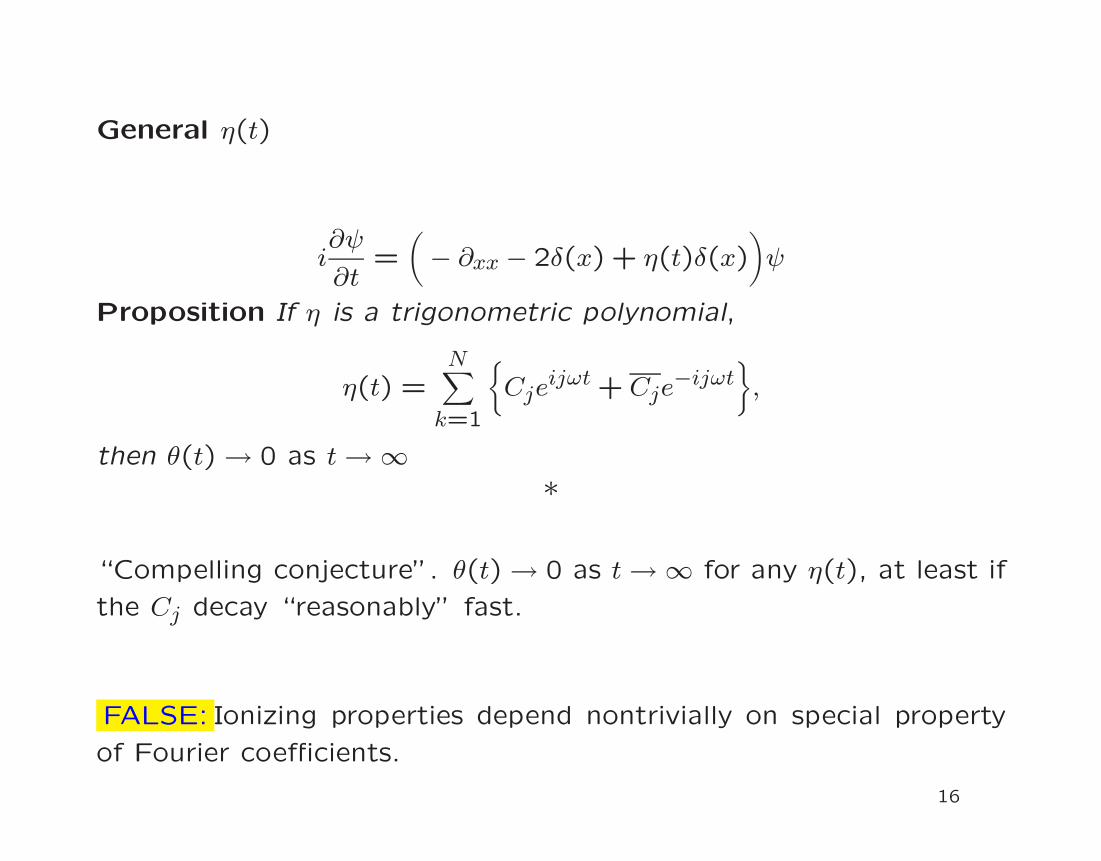
General η(t)

i∂ψ

∂t=

(

− ∂xx − 2δ(x) + η(t)δ(x)

)

ψ

Proposition If η is a trigonometric polynomial,

η(t) =N∑

k=1

Cjeijωt + Cje

−ijωt

,

then θ(t) → 0 as t→ ∞*

“Compelling conjecture”. θ(t) → 0 as t→ ∞ for any η(t), at least if

the Cj decay “reasonably” fast.

FALSE: Ionizing properties depend nontrivially on special property

of Fourier coefficients.

16

Consider a general periodic η(t)

η =∞∑

j=1

(

Cjeiωjt + C−je−iωjt

)

Genericity condition (g) The right shift operator T on l2(N) is

given by

T(C1, C2, ..., Cn, ...) = (C2, C3, ..., Cn+1, ...)

We say that C ∈ l2(N) is generic with respect to T if the Hilbert

space generated by all the translates of C contains the vector e1 =

(1,0,0, ...) (which is the kernel of T):

e1 ∈∞∨

n=0

TnC (g)

where the right side denotes the closure of the space generated by

the TnC with n ≥ 0. This condition is generically satisfied.

17

A simple example which fails (g) is,

η(t) = 2rλλ− cos(ωt)

1 + λ2 − 2λ cos(ωt)

for some λ ∈ (0,1). Here Cn = −rλn for n ≥ 1.

Theorem limt→∞

|θ(t)|=0, for all η satisfying (g)

Theorem For η with any ω, r there exists λ for which lim inft→∞

|θ(t)|>0.

1. There are infinitely many λ’s, accumulating at 1, such that

lim inft→∞

|θ(t)| > 0.

2. For large t, θ approaches a quasiperiodic function. Floquet

operator has a discrete spectrum, in this case.

3. This is nonperturbative. η(t) cannot be made arbitrarly small .

18

We have also investigated the case when

V0 = −δ(x), V1(x, t) = r [δ(x− a) + δ(x+ a)] sinωt

This also exhibits ”stabilization”. In fact one can find a two di-

mensional set of r, ω and a for which ionization fails. This is again

nonperturbative.

Surprise: Even when V0(x) = 0, so that there are no bound states,

we can find parameter values r, ω and a such that for an initial

ψ0 ∈ L2(R) the particle remain localized While this type of behavior

is probably peculiar to V1(x, t) consisting of delta functions there are

examples of systems with smooth V0 and V1 which fail to ionize. Still,

in this problem, proofs are necessary to convince even a ”reasonable”

person.

19

I describe now a very special model. Results are a bit more general.

Let χD(x) be the characteristic function of an arbitrary compact

set D in Rd, d=1,2,3. Set

V0(x) = r0χD(x), V1(x, t) = r1χD(x)sin(ωt)

Assume also that ψ0(x) = 0 for x ∈ D. Then

ψ(x, t) =∑

jǫZ

eijωthj(x, t) +∑

k=1

Pk(t)e−iσktFk(x, t),

with Imσk < 0 for all k. The Pk(t) are polynomials in t, and the

hj(x, t) have Borel summable power series in t−1/2 beginning with

t−3/2.

20

Dipole case in one dimension(O. Costin, JLL, C. Stucchio, RMP,

2008)

We consider the time evolution of a particle in one dimension gov-

erned by the Schrodinger equation with a delta function attractive

potential and a time-periodic dipole field:

i∂tψ(x, t) =

(

− ∂2

∂x2− 2δ(x)

)

ψ(x, t) +E(t)xψ(x, t)

ψ(x,0) = ψ0(x) ∈ L2(R)

This is a model used by physicists to study ionization. Our results

are the first ones (as far as we know) which actually prove ionization

for arbitrary strength fields.

21

Theorem 1. (Ionization) Suppose E(t) is a trigonometric polyno-

mial, i.e.

E(t) =N∑

n=1

(

Eneinωt + Ene

−inωt) .

Then for any ψ0(x) ∈ L2(R) ionization occurs, i.e.

limt→∞

∫ L

−L|ψ(x, t)|2dx = 0,∀L ∈ R

+

If ψ0(x) ∈ L1(R) ∩ L2(R), then the approach to zero is at least as

fast as t−1.

22

Theorem 2

Suppose ψ0(x) is compactly supported and in H1 and E(t) is smooth

and time periodic. Then, the solution ψ(x, t) can be uniquely (for

fixed M) decomposed as:

ψ(x, t) =M∑

k=0

nk∑

j=0

αk,jtje−iσktΦk,j(x, t) + ΨM(x, t)

The resonance energies σk satisfy ℑσk ≤ 0, and are ordered according

to ℑσk+1 ≤ ℑσk. The resonant states (φk,j(x, t)) are Gamow vectors

(generalized, if j > 0).

In the above expansion, we collect the M resonances with ℑσk clos-

est to zero, and M must be large enough so that we collect all

resonances σk with ℑσk = 0. The number of Gamow vectors (and

resonances) may be infinite, but we can only include finitely many

of them.

23

The remainder ΨM(x, t) has the following asymptotic expansion in

time:

ΨM(x, t) ∼∑

j∈Z

eijωt∞∑

n=1

Dj,n(x)t−n/2

This expansion is uniform on compact sets in x, but not in L2. In

general, Dj,n(x) is not in L2.

Uniqueness of the decomposition is defined relative to the analytic

structure of ψ(x, t): the Zak transform of ψ(x, t) has poles at σ = σk(with residues proportional to Φk,j(x, t)), while ΨM(x, t) has a Zak

transform that is analytic in the region σ : ℜσ ∈ (0, ω),ℑσ > ℑσM.The Zak transform is defined as follows.

24

Definition

Let f(t) = 0 for t < 0 and |f(t)| ≤ Ceαt for some α > 0. Then f(t) is

said to be Zak transformable. The Zak transform of f(t) is defined

(for ℑσ > α) by:

Z[f ](σ, t) =∑

j∈Z

eiσ(t+2πj/ω)f(t+ 2πj/ω)

We define y(σ, t) as the Zak transform of (essentially) the wave

function ψ(x, t) at x = c(t) where c′′(t) = 2E(t)

y(σ, t) is then given by:

y(σ, t) = [1 −K(σ)]−1y0(σ, t)

where y0(σ, t) is known, and K(σ) is a compact integral operator.

25

The poles of [1 − K(σ)]−1 correspond to the resonances σk in the

decomposition of ψ(x, t) while the φk,j(x, t) are related to the residues

at the poles of multiplicity j. They satisfy the equations,

(K − σk)φk,j = φk,j−1, φk,−1 = 0

with ’outgoing wave” or radiation boundary conditions: φk,0(x, t)

must behave like the Green’s function near |x| = ∞.

26

Coulomb systems in 3D (O. Costin, S. Tanveer, in preparation)

H = −∆ − b/r+ V (t, x) = HC + V, x ∈ R3, b > 0,

iψt = HCψ+ V (t, x)ψ; ψ(0, x) = ψ0(x) ∈ H1(R3)

where V (t, x) =∑∞j=1[Ωj(x)e

ijωt + c.c.]

Assumptions: Ωj(x), j ∈ Z have a common compact support, cho-

sen to be the ball B1 ⊂ R3 of radius 1, and∑

j∈Z (1 + |j|) ‖ Ωj ‖L2 (B1) <∞.

27

The homogeneous equation satisfied by the time Laplace transform

ψ(p, x) can be written (after some doctoring) as an infinite system

of second order equations (see slide 8)

(HC − ip1 + nω)wn = −∑

j∈Z

Ωj(x)wn−j,

where

p = p1 + inω, with p1 ∈ C mod iω.

28

Using rigorous WKB analysis of infinite systems of differential equa-

tions we show the following.

Theorem 1

For V (t, x) = 2Ω(r) sin(ωt−θ), with Ω(r) = 0 for r > 1, Ω(r) > 0 for

r ≤ 1 and Ω(r) ∈ C∞[0,1], σd(K) = ∅ and ionization always occurs.

Furthermore, if ψ0(x) is compactly supported and has only finitely

many spherical harmonics, then∫

B |ψ|2dx is O(t−5/3).

The proof, uses Theorems (2) and (3) and rigorous asymptotics of

wn as n→ −∞.

29

Theorem 2 Assuming spherical symmetry of the Ωj(x), ionization

occurs iff for all p1 ∈ iR, the homogeneous equation has only the

trivial solution wnn∈Z = 0 in the appropriate Hilbert space. This

is true iff σd(K) = ∅.

This extends results about absence of singular continuous spectrum

of the Floquet operator K, to this class of systems, with Coulombic

potential and spherical forcings of compact support.

30

Properties of Floquet bound states for general compactly

supported V (t, x).

Theorem 3 If there exists a nonzero solution of the homogeneous

equation, w ∈ H, then w has the further property

wn = χB1wn for all n < 0

with χA the characteristic function of the set A.

This makes the second order homogeneous system formally overde-

termined since the regularity of w in x imposes both Dirichlet and

Neumann conditions on ∂B1 for n < 0. Nontrivial solutions are not,

in general, expected to exist.

31

Remark

The results can be extended to systems with HC replaced by

HW = −∆− b/r+W (r)

where b may be zero and W (r) decays at least as fast as r−1−ǫ for

large r, W ∈ L∞(R3).

32

Outline of the ideas entering proof As in our previous work on

simpler systems, we rely on a modified Fredholm theory to prove

a dichotomy: either there are bound Floquet states, or the system

gets ionized. Mathematically the Coulomb potential introduces a

number of substantial difficulties compared to the potentials con-

sidered before due to its singular behavior at the origin and, more

importantly, its very slow decay at infinity.

The slow decay translates into potential-specific corrections at in-

finity and the asymptotic behavior in the far field of the resolvent

has to be calculated in detail The accumulation of eigenvalues of

increasing multiplicity at the top of the discrete spectrum of HC pro-

duces an essential singularity at zero of the Floquet resolvent. This

is responsible for the change in the large time asymptotic behavior

of the wave function, from t−3/2 to t−5/6.

33