ion transport through biological cell membranes: from...
TRANSCRIPT
Ion Transport through Biological Cell Membranes:
From Electro-Diffusion to Hodgkin−Huxley via a Quasi
Steady-State Approach
Viktoria R.T. Hsu
A dissertation submitted in partial fulfillment
of the requirements for the degree of
Doctor of Philosophy
University of Washington
2004
Program Authorized to Offer Degree: Applied Mathematics

University of Washington
Graduate School
This is to certify that I have examined this copy of a doctoral dissertation by
Viktoria R.T. Hsu
and have found that it is complete and satisfactory in all respects,
and that any and all revisions required by the final
examining committee have been made.
Chair of Supervisory Committee:
Hong Qian
Reading Committee:
Hong Qian
Mark Kot
David Perkel
Date:

In presenting this dissertation in partial fulfillment of the requirements for the Doc-
toral degree at the University of Washington, I agree that the Library shall make
its copies freely available for inspection. I further agree that extensive copying of
this dissertation is allowable only for scholarly purposes, consistent with “fair use” as
prescribed in the U.S. Copyright Law. Requests for copying or reproduction of this
dissertation may be referred to Bell and Howell Information and Learning, 300 North
Zeeb Road, Ann Arbor, MI 48106-1346, to whom the author has granted “the right
to reproduce and sell (a) copies of the manuscript in microform and/or (b) printed
copies of the manuscript made from microform.”
Signature
Date

University of Washington
Abstract
Ion Transport through Biological Cell Membranes:
From Electro-Diffusion to Hodgkin−Huxley via a Quasi Steady-State
Approach
by Viktoria R.T. Hsu
Chair of Supervisory Committee:
Professor Hong QianApplied Mathematics
Biological cells in tissue are in close proximity to neighboring cells and share a rela-
tively small external environment. Ion concentrations in and the size of this external
space vary significantly during conditions such as epileptic seizures or heart attacks.
Hodgkin−Huxley-type models to date incorporate variable internal concentrations
but static cell volume and external concentrations. In this sense, more accurate math-
ematical models of cells in tissue are needed. We extend current Hodgkin−Huxley-
type models toward a mathematical model of a single-cell micro-environment incor-
porating variable external concentrations and variable cell volume. Variable external
concentrations require a finite volume of the external compartment. Thus, mass con-
servation and electroneutrality need to hold for the entire, finite-volume system. This
means, in particular, that a phenomenological approach neglecting electroneutrality
may not be adopted, if we want a more physically grounded representation of the
ionic fluxes and cross-membrane potential than current Hodgkin−Huxley-type mod-
els offer. The development of our model addresses this issue in detail.

TABLE OF CONTENTS
List of Figures v
List of Tables viii
Chapter 1: Review of Neuron Modeling 1
1.1 The Brain and its Neurons . . . . . . . . . . . . . . . . . . . . . . . . 1
1.1.1 Anatomic Structure of the Human Brain . . . . . . . . . . . . 1
1.1.2 The Hippocampus . . . . . . . . . . . . . . . . . . . . . . . . 3
1.1.3 Neuron and Glia Cells . . . . . . . . . . . . . . . . . . . . . . 3
1.2 Signaling and the Role of Ionic Species . . . . . . . . . . . . . . . . . 7
1.2.1 Inhibition versus Excitation . . . . . . . . . . . . . . . . . . . 7
1.2.2 Ion Species and Their Relevance . . . . . . . . . . . . . . . . . 9
1.2.3 Important Ion Species in Detail . . . . . . . . . . . . . . . . . 11
1.3 Introduction to Hodgkin−Huxley Theory . . . . . . . . . . . . . . . 15
1.3.1 The Classic Hodgkin−Huxley Model . . . . . . . . . . . . . . 16
1.3.2 An Overview of Mathematical Neuron Models . . . . . . . . . 20
1.4 Limitations of Current Models in Tissue Modeling . . . . . . . . . . 25
1.4.1 Reflection on Problems with Current Models . . . . . . . . . . 26
1.5 Toward Biophysically Consistent Tissue Modeling . . . . . . . . . . . 28
Chapter 2: Ion Transport by Electro-Diffusion 32
2.1 Setup and Assumptions for Simulating Electro-Diffusion and Poisson
Equations . . . . . . . . . . . . . . . . . . . . . . . . . . . . . . . . . 33
i
2.1.1 Flux Conditions for Impermeant Species . . . . . . . . . . . . 37
2.1.2 Boundary Conditions for the Electrostatic Potential . . . . . . 38
2.2 The Quasi Steady-State Approximation (QSSA) and Relaxation Times
to Donnan Equilibrium . . . . . . . . . . . . . . . . . . . . . . . . . . 41
2.2.1 Spatially Constant Bulk Concentrations . . . . . . . . . . . . 43
2.2.2 Membrane Region at Steady-State . . . . . . . . . . . . . . . 43
2.2.3 QSSA for Relaxation to Donnan Equilibrium . . . . . . . . . . 44
2.2.4 Relaxation Times . . . . . . . . . . . . . . . . . . . . . . . . . 45
2.2.5 Comparison of Analytic and Numeric Approximations . . . . . 46
2.3 Analytic Equilibrium Solutions to the 1D Electro-Diffusion System . 47
2.3.1 Boundary Conditions at Donnan Equilibrium . . . . . . . . . 51
2.3.2 Equilibrium Solution With Valency j=-2 in the System . . . . 56
2.3.3 Equilibrium Solution Without Valency j=-2 in the System . . 62
Chapter 3: Dynamic Approach to Donnan Equilibrium 66
3.1 Numeric Solution of Transient Electro-Diffusion System . . . . . . . 66
3.1.1 Discretization of the Domain . . . . . . . . . . . . . . . . . . . 67
3.1.2 Solving Poisson’s Equation . . . . . . . . . . . . . . . . . . . . 68
3.1.3 Flux Densities from Electro-Diffusion Equations . . . . . . . . 70
3.1.4 Updating Concentrations by Various Solution Schemes . . . . 71
3.1.5 Time-Step Restrictions and Numeric Diffusion . . . . . . . . . 74
3.2 Numeric Solution of the Steady-State Problem Using an “Almost-
Newton” Method . . . . . . . . . . . . . . . . . . . . . . . . . . . . . 76
3.2.1 Full Newton Method. . . . . . . . . . . . . . . . . . . . . . . . 79
3.2.2 Gummel Method. . . . . . . . . . . . . . . . . . . . . . . . . . 80
3.2.3 Almost-Newton Method. . . . . . . . . . . . . . . . . . . . . . 83
3.2.4 Comparison of Iterative Methods. . . . . . . . . . . . . . . . . 85
ii
3.3 Numeric Simulation of the Quasi Steady-State Approximation . . . . 91
3.3.1 Implementation of the QSSA . . . . . . . . . . . . . . . . . . 92
3.3.2 Dynamics of PDE Compared to Approximation of Dynamics
by QSSA . . . . . . . . . . . . . . . . . . . . . . . . . . . . . . 93
3.4 Summary of Results . . . . . . . . . . . . . . . . . . . . . . . . . . . 94
Chapter 4: From QSSA to the classic Hodgkin−Huxley model 99
4.1 Adjusting to end-of-membrane impermeability . . . . . . . . . . . . . 99
4.2 Constant field approximation of the QSSA . . . . . . . . . . . . . . . 101
4.2.1 Derivation of the constant field approximation (CFA) . . . . 102
4.2.2 Numerical comparison of QSSA and CFA . . . . . . . . . . . . 106
4.3 Linearization of the QSSA: the HH-plk Model . . . . . . . . . . . . . 120
4.4 Dynamic approach to the equilibrium of a cell . . . . . . . . . . . . . 122
4.5 Sustaining the living state of a cell . . . . . . . . . . . . . . . . . . . 130
4.5.1 Simple model for ion pump currents . . . . . . . . . . . . . . 131
4.5.2 Numerical simulations and results . . . . . . . . . . . . . . . 133
4.6 Summary of Results . . . . . . . . . . . . . . . . . . . . . . . . . . . 138
Chapter 5: Conclusions and Future Work 141
5.1 Future Work . . . . . . . . . . . . . . . . . . . . . . . . . . . . . . . . 143
Glossary 145
Bibliography 147
Appendix A: Dynamic Equations for Volume Change 156
A.1 Cell volume and cell surface area . . . . . . . . . . . . . . . . . . . . 156
A.1.1 Elastic cell membrane . . . . . . . . . . . . . . . . . . . . . . 158
A.1.2 Cell membrane with constant surface area . . . . . . . . . . . 159
iii
A.2 Cell volume dynamics . . . . . . . . . . . . . . . . . . . . . . . . . . . 162
A.3 Concentration dynamics . . . . . . . . . . . . . . . . . . . . . . . . . 163
Appendix B: Modeling Sophisticated Channels and Active Transport165
B.1 Channels and Pumps in the CFA framework . . . . . . . . . . . . . . 165
B.1.1 Diffusion coefficients in lipid membrane . . . . . . . . . . . . . 166
B.1.2 Diffusion coefficients in solute filled pores . . . . . . . . . . . . 168
B.1.3 Pump fluxes . . . . . . . . . . . . . . . . . . . . . . . . . . . . 171
B.1.4 Calcium sensitivity . . . . . . . . . . . . . . . . . . . . . . . . 172
B.1.5 Volume dynamics via flux of water . . . . . . . . . . . . . . . 174
B.2 Including source terms in the QSSA . . . . . . . . . . . . . . . . . . . 176
Appendix C: Epilepsy: An Introduction 180
C.1 Pathology and Medical Treatment . . . . . . . . . . . . . . . . . . . . 181
C.2 Definition of Epilepsy in Vivo . . . . . . . . . . . . . . . . . . . . . . 183
C.3 Definition of Epilepsy in Vitro . . . . . . . . . . . . . . . . . . . . . . 187
C.4 Relevant Knowledge About Epileptic Neuron . . . . . . . . . . . . . . 188
C.5 Nonlinear Dynamics and Epilepsy . . . . . . . . . . . . . . . . . . . . 190
Appendix D: Integrals of Equilibrium Solutions 192
D.1 Integrals in case of a mono-valent system . . . . . . . . . . . . . . . . 194
D.2 Integrals in case no valency j = −2 is present . . . . . . . . . . . . . 195
D.3 Integrals in case valency j = −2 is present and u1 6= u2 . . . . . . . . 197
iv
LIST OF FIGURES
1.1 Lobes of the human brain. . . . . . . . . . . . . . . . . . . . . . . . . 2
1.2 Limbic system of the human brain. . . . . . . . . . . . . . . . . . . . 2
1.3 Hippocampal slice preparation. . . . . . . . . . . . . . . . . . . . . . 4
1.4 Pyramidal neuron and Purkinje cell. . . . . . . . . . . . . . . . . . . 5
1.5 A neuron cell and its components. . . . . . . . . . . . . . . . . . . . . 6
1.6 Flow of information along different types of neurons. . . . . . . . . . 6
1.7 Signal following stimulus for non-excitable and excitable cell. . . . . . 8
1.8 Coupling circuit of inhibitory and excitatory neuron. . . . . . . . . . 9
1.9 Sodium and potassium channels shape the action potential. . . . . . . 10
1.10 Schematic of leaky capacitor. . . . . . . . . . . . . . . . . . . . . . . 17
1.11 Fast-slow phase-plane, flow directions. . . . . . . . . . . . . . . . . . 19
1.12 Fast-slow phase-plane, sub-threshold stimulus. . . . . . . . . . . . . . 20
1.13 Fast-slow phase-plane, super-threshold stimulus. . . . . . . . . . . . . 21
2.1 A cell and its environment. . . . . . . . . . . . . . . . . . . . . . . . . 35
2.2 Domain in 1D, zero flux at mid-membrane. . . . . . . . . . . . . . . . 39
2.3 Chart of charge-carrier transport in various backgrounds. . . . . . . . 40
2.4 Comparison of PDE to approximation with relaxation constant. . . . 47
3.1 Discretized, mathematical domain. . . . . . . . . . . . . . . . . . . . 68
3.2 Grid refinement at equilibrium. . . . . . . . . . . . . . . . . . . . . . 86
3.3 Number of iterations needed for convergence of MG, FN, and AN. . . 87
3.4 Maximum absolute residual for MG, FN and AN. . . . . . . . . . . . 88
v

3.5 Estimate of absolute relative error in for MG, FN and AN. . . . . . . 89
3.6 QSSA vs. PDE initialized with piecewise constant initial condition. . 95
3.7 QSSA and PDE initialized at non-equilibrium steady-state. . . . . . . 96
3.8 QSSA and PDE initialized at far-from-equilibrium steady-state. . . . 97
4.1 Domain for end of membrane impermeability. . . . . . . . . . . . . . 100
4.2 Steady-state concentration profiles, no protein. . . . . . . . . . . . . . 108
4.3 steady-state and CFA potential profiles, no protein. . . . . . . . . . . 109
4.4 Steady-state and equilibrium bulk profiles, no protein. . . . . . . . . . 109
4.5 Error in equilibrium potential profiles at steady-state, no protein. . . 110
4.6 Steady-state concentration profiles, protein internal bulk. . . . . . . . 112
4.7 Steady-state and CFA potential profiles, protein internal bulk. . . . . 113
4.8 Steady-state and eqlb. bulk profiles, protein internal bulk. . . . . . . 113
4.9 Error in eqlb. potential profiles at steady-state, protein internal bulk. 114
4.10 Steady-state concentration profiles, protein both bulks. . . . . . . . . 116
4.11 Steady-state and CFA potential profiles, protein both bulks. . . . . . 117
4.12 Steady-state and equilibrium bulk profiles, protein both bulks. . . . . 117
4.13 Error in equilibrium potential profiles at steady-state, protein both bulks.118
4.14 To death: Concentration dynamics. . . . . . . . . . . . . . . . . . . . 124
4.15 To death: Current density dynamics. . . . . . . . . . . . . . . . . . . 125
4.16 To death: Potential dynamics. . . . . . . . . . . . . . . . . . . . . . . 126
4.17 To death: Measure for EN self-regulation. . . . . . . . . . . . . . . . 128
4.18 To death: Rel. measure for EN self-regulation. . . . . . . . . . . . . . 129
4.19 Resting state of HH maintained by CFA and HHplk. . . . . . . . . . 133
4.20 Relative measure for EN self-regulation at rest. . . . . . . . . . . . . 134
4.21 Action potential by CFA, HHplk, and classic HH models. . . . . . . . 135
4.22 Current densities for action potential by CFA, HHplk, and classic HH. 136
vi
4.23 Relative measure of EN self-regulation during an action potential. . . 137
A.1 Schema of cell with elastic membrane surface area. . . . . . . . . . . 157
A.2 Schema of cell with constant membrane surface area. . . . . . . . . . 160
C.1 Routine and epileptic EEG. . . . . . . . . . . . . . . . . . . . . . . . 185
vii
LIST OF TABLES
2.1 Appropriate sign combinations according to the net charge in each
region of the domain. . . . . . . . . . . . . . . . . . . . . . . . . . . . 58
B.1 Permeability coefficients for membrane of human erythrocyte. . . . . 167
B.2 Equivalent conductivities. . . . . . . . . . . . . . . . . . . . . . . . . 170
viii
ACKNOWLEDGMENTS
The author expresses her sincere appreciation to her thesis advisor, Hong Qian,
for supporting an idea outside of his primary interests and for helping to form this
idea into something exciting and meaningful. This work would not have been possible
without him.
The author further expresses her appreciation to her thesis advising committee
consisting of Hong Qian, Mark Kot, David Perkel, Nathan Kutz, and Loyce Adams
for their qualified advice, patience, and dedicated personal support in all matters.
Special thanks are also extended to Bob O’Malley and to John Chadam for their
friendly support, helpful advice, and interest in the author’s personal and academic
where-abouts.
The author expresses her gratitude to the GK-12 outreach program under NSF
grant number DGE-0086280, to the Departments of Mathematics and Applied Math-
ematics at the University of Washington, to the German National Merit Scholarship
Foundation (Studienstiftung des deutschen Volkes, e.V.), in particular, to Dr. Strub-
Rottgerding, and to the Fachbereich 11 Mathematik at the Universitat-GH Duisburg,
in particular, professors Eberhard, Freiling, Schreckenberg,and Torner for their in-
valuable contributions to her professional development and their financial support
during her time as a graduate student.
ix

DEDICATION
Fur meine Familie, insbesondere
meine Eltern, Großeltern und Ingrid “Ingi” Sobbing,
fur deren Unterstutzung meine Worte nicht ausreichen.
For my husband, Terry,
for making sure that I eat my veggies and
for every other detail that does not fit onto this page.
To my friends in the new and the old world,
who have provided me with an unbeatable support system.
Fur Hartmut Kranenberg, der als Erster
ernsthaft vorschlug ich solle Mathematik studieren.
x
1
Chapter 1
REVIEW OF NEURON MODELING
Before introducing existing, deterministic neuron models in section 1.3, we should
understand some basic properties of the brain and its cells, known as neurons. Thus,
a broad introduction to the anatomic structure of the human brain and its neurons is
given in section 1.1 and an overview of basic signaling principles and their underlying
mechanisms is provided in section 1.2. Current, Hodgkin−Huxley-type mathematical
neuron models are introduced on this foundation in section 1.3.
In the second part of this introductory chapter, the limitations of current neuron
models with respect to “in tissue” modeling are discussed in section 1.4 and followed
by a proposal for overcoming these limitations in section 1.5. As such, section 1.5
serves as an outline for the remainder of this dissertation.
1.1 The Brain and its Neurons
1.1.1 Anatomic Structure of the Human Brain
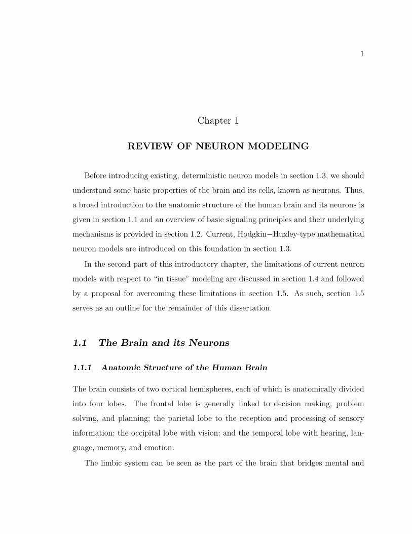
The brain consists of two cortical hemispheres, each of which is anatomically divided
into four lobes. The frontal lobe is generally linked to decision making, problem
solving, and planning; the parietal lobe to the reception and processing of sensory
information; the occipital lobe with vision; and the temporal lobe with hearing, lan-
guage, memory, and emotion.
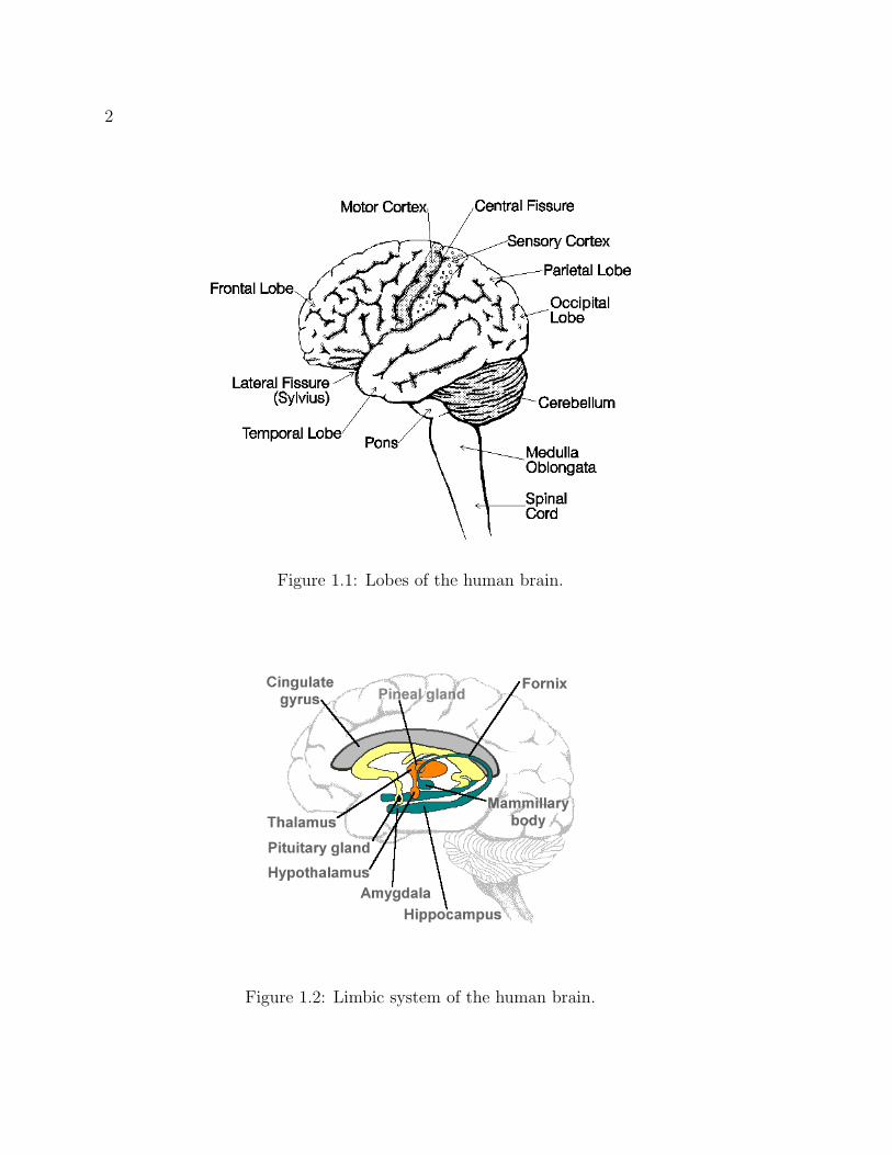
The limbic system can be seen as the part of the brain that bridges mental and
2
Figure 1.1: Lobes of the human brain.
Figure 1.2: Limbic system of the human brain.
3
physical states, as it is located between the cortex and the mid-brain. Although the
sensory and motor regions link the central nervous system (brain and spinal cord)
with the body, the activity of the limbic system allows the brain to regulate and alter
the body’s internal environment by means of hormonal and other controls. The limbic
system also allows cognition, senses, and physical reactions to join together in every-
day experience and to be retained in various forms of memory. The hippocampus,
in particular, is believed to play a crucial role in the formation and retaining of long
term memory. It is located along the cores of the temporal lobes and is the subject of
many studies. Its structure and function will be given more attention in the following
section.
1.1.2 The Hippocampus
The hippocampus has a relatively simple morphological structure compared to other
regions of the brain. For example, the cortex has six distinct and functionally differ-
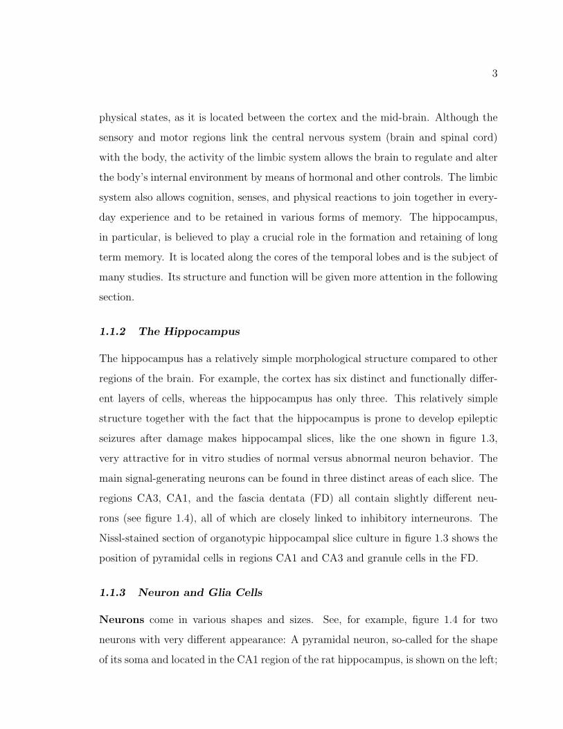
ent layers of cells, whereas the hippocampus has only three. This relatively simple
structure together with the fact that the hippocampus is prone to develop epileptic
seizures after damage makes hippocampal slices, like the one shown in figure 1.3,
very attractive for in vitro studies of normal versus abnormal neuron behavior. The
main signal-generating neurons can be found in three distinct areas of each slice. The
regions CA3, CA1, and the fascia dentata (FD) all contain slightly different neu-
rons (see figure 1.4), all of which are closely linked to inhibitory interneurons. The
Nissl-stained section of organotypic hippocampal slice culture in figure 1.3 shows the
position of pyramidal cells in regions CA1 and CA3 and granule cells in the FD.
1.1.3 Neuron and Glia Cells
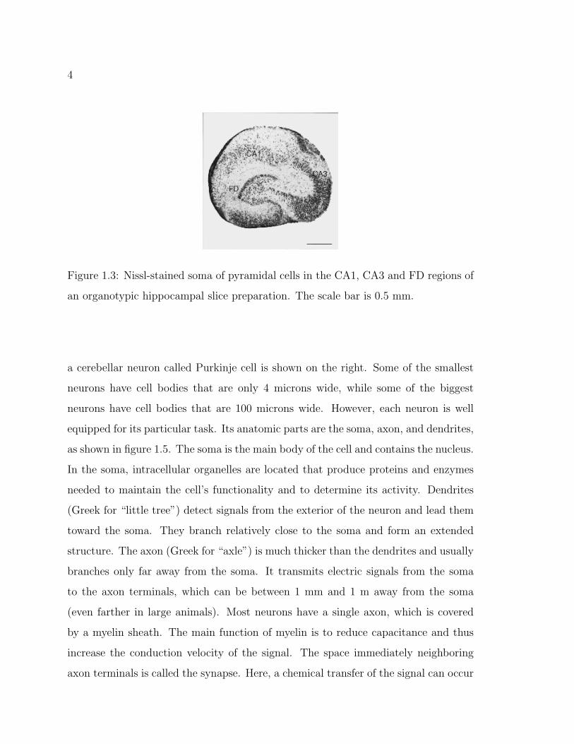
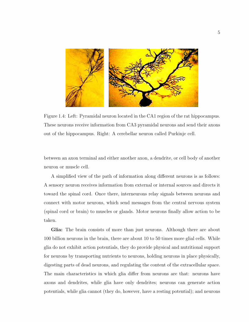
Neurons come in various shapes and sizes. See, for example, figure 1.4 for two
neurons with very different appearance: A pyramidal neuron, so-called for the shape
of its soma and located in the CA1 region of the rat hippocampus, is shown on the left;
4
Figure 1.3: Nissl-stained soma of pyramidal cells in the CA1, CA3 and FD regions of
an organotypic hippocampal slice preparation. The scale bar is 0.5 mm.
a cerebellar neuron called Purkinje cell is shown on the right. Some of the smallest
neurons have cell bodies that are only 4 microns wide, while some of the biggest
neurons have cell bodies that are 100 microns wide. However, each neuron is well
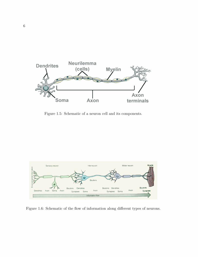
equipped for its particular task. Its anatomic parts are the soma, axon, and dendrites,
as shown in figure 1.5. The soma is the main body of the cell and contains the nucleus.
In the soma, intracellular organelles are located that produce proteins and enzymes
needed to maintain the cell’s functionality and to determine its activity. Dendrites
(Greek for “little tree”) detect signals from the exterior of the neuron and lead them
toward the soma. They branch relatively close to the soma and form an extended
structure. The axon (Greek for “axle”) is much thicker than the dendrites and usually
branches only far away from the soma. It transmits electric signals from the soma
to the axon terminals, which can be between 1 mm and 1 m away from the soma
(even farther in large animals). Most neurons have a single axon, which is covered
by a myelin sheath. The main function of myelin is to reduce capacitance and thus
increase the conduction velocity of the signal. The space immediately neighboring
axon terminals is called the synapse. Here, a chemical transfer of the signal can occur
5
Figure 1.4: Left: Pyramidal neuron located in the CA1 region of the rat hippocampus.
These neurons receive information from CA3 pyramidal neurons and send their axons
out of the hippocampus. Right: A cerebellar neuron called Purkinje cell.
between an axon terminal and either another axon, a dendrite, or cell body of another
neuron or muscle cell.
A simplified view of the path of information along different neurons is as follows:
A sensory neuron receives information from external or internal sources and directs it
toward the spinal cord. Once there, interneurons relay signals between neurons and
connect with motor neurons, which send messages from the central nervous system
(spinal cord or brain) to muscles or glands. Motor neurons finally allow action to be
taken.
Glia: The brain consists of more than just neurons. Although there are about
100 billion neurons in the brain, there are about 10 to 50 times more glial cells. While
glia do not exhibit action potentials, they do provide physical and nutritional support
for neurons by transporting nutrients to neurons, holding neurons in place physically,
digesting parts of dead neurons, and regulating the content of the extracellular space.
The main characteristics in which glia differ from neurons are that: neurons have
axons and dendrites, while glia have only dendrites; neurons can generate action
potentials, while glia cannot (they do, however, have a resting potential); and neurons
6
Figure 1.5: Schematic of a neuron cell and its components.
Figure 1.6: Schematic of the flow of information along different types of neurons.
7
have chemical synapses using neurotransmitters, while glia do not have any chemical
synapses.
1.2 Signaling and the Role of Ionic Species
1.2.1 Inhibition versus Excitation
Two important and very basic features of communication between neurons are inhi-
bition and excitation. In fact, excitability is what distinguishes neurons and muscle
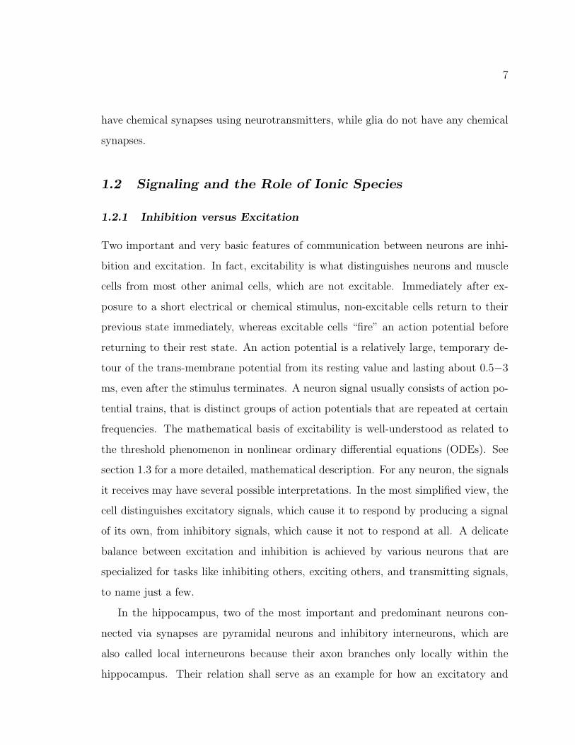
cells from most other animal cells, which are not excitable. Immediately after ex-
posure to a short electrical or chemical stimulus, non-excitable cells return to their
previous state immediately, whereas excitable cells “fire” an action potential before
returning to their rest state. An action potential is a relatively large, temporary de-
tour of the trans-membrane potential from its resting value and lasting about 0.5−3
ms, even after the stimulus terminates. A neuron signal usually consists of action po-
tential trains, that is distinct groups of action potentials that are repeated at certain
frequencies. The mathematical basis of excitability is well-understood as related to
the threshold phenomenon in nonlinear ordinary differential equations (ODEs). See
section 1.3 for a more detailed, mathematical description. For any neuron, the signals
it receives may have several possible interpretations. In the most simplified view, the
cell distinguishes excitatory signals, which cause it to respond by producing a signal
of its own, from inhibitory signals, which cause it not to respond at all. A delicate
balance between excitation and inhibition is achieved by various neurons that are
specialized for tasks like inhibiting others, exciting others, and transmitting signals,
to name just a few.
In the hippocampus, two of the most important and predominant neurons con-
nected via synapses are pyramidal neurons and inhibitory interneurons, which are
also called local interneurons because their axon branches only locally within the
hippocampus. Their relation shall serve as an example for how an excitatory and
8
Figure 1.7: Voltage vs. time; trans-membrane voltage returns to resting value imme-
diately following a stimulus for a non-excitable cell but exhibits a large detour from
the resting state (action potential) for an excitable cell before returning to the resting
value.
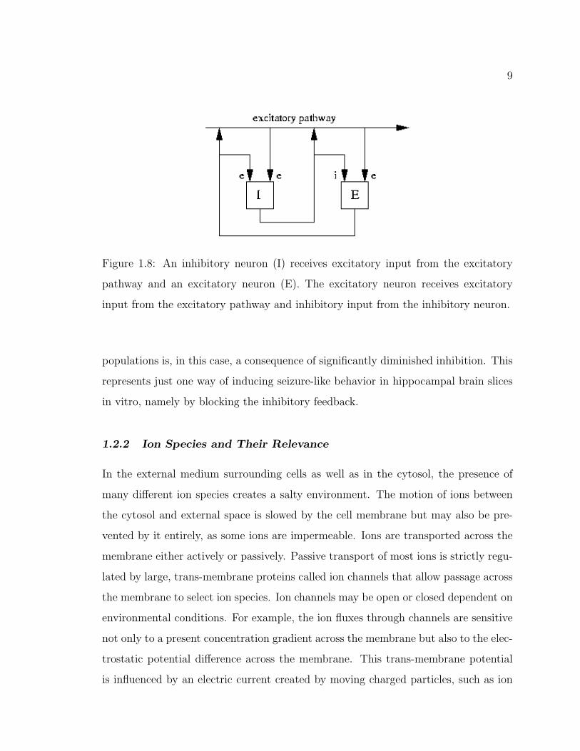
inhibitory balance is believed to function in the most basic way (see figure 1.8 for
a schematic). Each type of neuron receives two different input signals and produces
one output signal. For both cell types, one input signal originates from the excitatory
pathway, which may be viewed as a collective signal from the surrounding tissue.
The second input comes from the output of the other neuron type. This output,
as just indicated, is connected to the input of its counterpart but also contributes
to the excitatory pathway. As its name indicates, the excitatory pathway excites
both types of cells, such that the inhibitory neuron is excited by both of its inputs,
whereas the pyramidal neuron is excited by the excitatory pathway and inhibited by
the interneuron. Hence, the more excited the pyramidal cell is, the more inhibition it
will ultimately receive from the interneuron. The damage of inhibitory interneurons
is thus believed to enable the occurrence of hyper-excited signals of the pyramidal
neurons.
The inhibitory interneurons of the hippocampus seem, in fact, particularly sensi-
tive to damage by trauma, such that the resulting hyper-excited response of pyramidal
9
Figure 1.8: An inhibitory neuron (I) receives excitatory input from the excitatory
pathway and an excitatory neuron (E). The excitatory neuron receives excitatory
input from the excitatory pathway and inhibitory input from the inhibitory neuron.
populations is, in this case, a consequence of significantly diminished inhibition. This
represents just one way of inducing seizure-like behavior in hippocampal brain slices
in vitro, namely by blocking the inhibitory feedback.
1.2.2 Ion Species and Their Relevance
In the external medium surrounding cells as well as in the cytosol, the presence of
many different ion species creates a salty environment. The motion of ions between
the cytosol and external space is slowed by the cell membrane but may also be pre-
vented by it entirely, as some ions are impermeable. Ions are transported across the
membrane either actively or passively. Passive transport of most ions is strictly regu-
lated by large, trans-membrane proteins called ion channels that allow passage across
the membrane to select ion species. Ion channels may be open or closed dependent on
environmental conditions. For example, the ion fluxes through channels are sensitive
not only to a present concentration gradient across the membrane but also to the elec-
trostatic potential difference across the membrane. This trans-membrane potential
is influenced by an electric current created by moving charged particles, such as ion
10
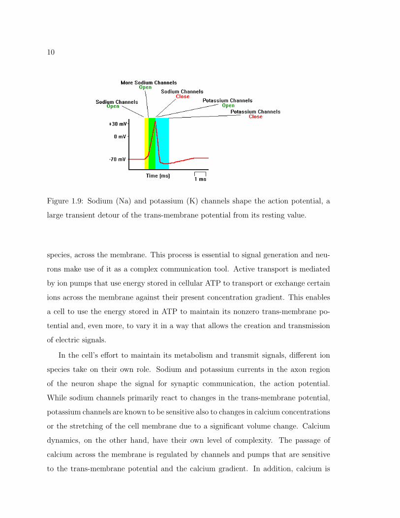
Figure 1.9: Sodium (Na) and potassium (K) channels shape the action potential, a
large transient detour of the trans-membrane potential from its resting value.
species, across the membrane. This process is essential to signal generation and neu-
rons make use of it as a complex communication tool. Active transport is mediated
by ion pumps that use energy stored in cellular ATP to transport or exchange certain
ions across the membrane against their present concentration gradient. This enables
a cell to use the energy stored in ATP to maintain its nonzero trans-membrane po-
tential and, even more, to vary it in a way that allows the creation and transmission
of electric signals.
In the cell’s effort to maintain its metabolism and transmit signals, different ion
species take on their own role. Sodium and potassium currents in the axon region
of the neuron shape the signal for synaptic communication, the action potential.
While sodium channels primarily react to changes in the trans-membrane potential,
potassium channels are known to be sensitive also to changes in calcium concentrations
or the stretching of the cell membrane due to a significant volume change. Calcium
dynamics, on the other hand, have their own level of complexity. The passage of
calcium across the membrane is regulated by channels and pumps that are sensitive
to the trans-membrane potential and the calcium gradient. In addition, calcium is
11
highly buffered in several separate compartments inside the cytosol, one of which is
called the endoplasmic reticulum (ER). The uptake into and release from the ER are
regulated by additional calcium pumps and channels.
Neurons maintain and regulate all these processes to maintain a stable volume
and to transmit information efficiently and effectively. It is clear that, for modeling
purposes, the large number of currents and ion species must be restricted. Therefore,
the most important problem for modeling at this time is to choose which currents
or ionic species to neglect. Two main criteria help decide which ion species and
currents to include: First, currents should be modeled that play a big role in the
transmission of signals and those closely related to them. Second, currents should be
excluded for which there is very little experimental data and for which no mechanisms
are known. Some of the transport mediators, ion species, and their corresponding
currents considered important in neurons will be introduced in more detail in the
following section.
1.2.3 Important Ion Species in Detail
Channels, Pumps, and Transporters
Channels, pumps, and transporters are complex proteins embedded in the cell mem-
brane that allow and control the movement of ion species across the membrane. They
can assume an open or closed state depending on the trans-membrane potential, con-
centration gradients, or other cellular messengers. Whereas channels generally medi-
ate transport for either one ion species or all ion species at once, transporters pass
at least two different species through the membrane. More specifically, transporters
exchange well-defined ratios of specific ion species such that one kind moves from the
inside to the outside while the other kind moves from the outside to the inside of
the cell. Further, two main types of transport are distinguished: Passive transport
due to electro-chemical gradients and active transport against such gradients at the
12
expense of energy. Passive transport occurs through selective or non-selective ion
channels or gradient-driven transporters. Some transporters also support the cell’s
active transport system by working as ion exchange pumps and using ATP to move
ions against a present electro-chemical gradient. More active transport is mediated
by plasma membrane pumps, which pump a single ion species against its chemical
gradient.
Some pumps and transporters are predominantly present in certain types of neu-
rons. In addition, pumps and transporters are often distributed differently in the
soma and dendritic regions of any given cell. This makes it hard to understand how
exactly the regulation of trans-membrane potential and volume work, especially since
different cell types have different morphological features, functions, and characteris-
tics in the network. However, membrane pumps working against chemical gradients
maintain the cell’s trans-membrane potential and play a significant role in keeping
the cell volume stable. In the latter function, they are supported by impermeant ions,
mentioned below.
Examples of transporters are electrogenic Na-K pumps in glia (3 Na out for each
2 K in), the gradient-driven Na-Ca exchanger (3 Na in for each 1 Ca out), and the
gradient-driven Na-K-Cl co-transporter in glia (1 Na in for each 1 K in and 2 Cl in).
There is literally any combination of Na-K-Ca-Cl transport present in human cells
and, in addition, some transporters move H (protons) or HCO3 (bicarbonate), which
influence the pH of the cell and its milieu. This has also been hypothesized to be
important in the regulation of trans-membrane potential and cell volume, however,
not much experimental data is available to date.
Potassium Channels
Potassium (K) channels operate according to two main mechanisms: Calcium (Ca)
sensitivity and voltage sensitivity. Because the cell maintains internal K high com-
pared to external K, these channels mostly leak K from the cytosol. Easily a dozen
13
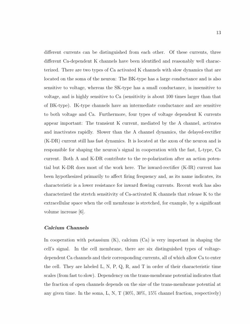
different currents can be distinguished from each other. Of these currents, three
different Ca-dependent K channels have been identified and reasonably well charac-
terized. There are two types of Ca activated K channels with slow dynamics that are
located on the soma of the neuron: The BK-type has a large conductance and is also
sensitive to voltage, whereas the SK-type has a small conductance, is insensitive to
voltage, and is highly sensitive to Ca (sensitivity is about 100 times larger than that
of BK-type). IK-type channels have an intermediate conductance and are sensitive
to both voltage and Ca. Furthermore, four types of voltage dependent K currents
appear important: The transient K current, mediated by the A channel, activates
and inactivates rapidly. Slower than the A channel dynamics, the delayed-rectifier
(K-DR) current still has fast dynamics. It is located at the axon of the neuron and is
responsible for shaping the neuron’s signal in cooperation with the fast, L-type, Ca
current. Both A and K-DR contribute to the re-polarization after an action poten-
tial but K-DR does most of the work here. The inward-rectifier (K-IR) current has
been hypothesized primarily to affect firing frequency and, as its name indicates, its
characteristic is a lower resistance for inward flowing currents. Recent work has also
characterized the stretch sensitivity of Ca-activated K channels that release K to the
extracellular space when the cell membrane is stretched, for example, by a significant
volume increase [6].
Calcium Channels
In cooperation with potassium (K), calcium (Ca) is very important in shaping the
cell’s signal. In the cell membrane, there are six distinguished types of voltage-
dependent Ca channels and their corresponding currents, all of which allow Ca to enter
the cell. They are labeled L, N, P, Q, R, and T in order of their characteristic time
scales (from fast to slow). Dependency on the trans-membrane potential indicates that
the fraction of open channels depends on the size of the trans-membrane potential at
any given time. In the soma, L, N, T (30%, 30%, 15% channel fraction, respectively)
14
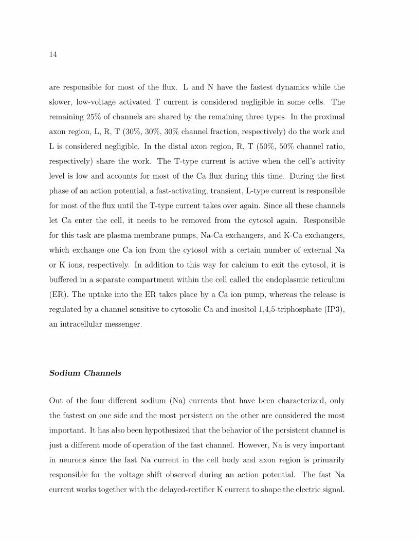
are responsible for most of the flux. L and N have the fastest dynamics while the
slower, low-voltage activated T current is considered negligible in some cells. The
remaining 25% of channels are shared by the remaining three types. In the proximal
axon region, L, R, T (30%, 30%, 30% channel fraction, respectively) do the work and
L is considered negligible. In the distal axon region, R, T (50%, 50% channel ratio,
respectively) share the work. The T-type current is active when the cell’s activity
level is low and accounts for most of the Ca flux during this time. During the first
phase of an action potential, a fast-activating, transient, L-type current is responsible
for most of the flux until the T-type current takes over again. Since all these channels
let Ca enter the cell, it needs to be removed from the cytosol again. Responsible
for this task are plasma membrane pumps, Na-Ca exchangers, and K-Ca exchangers,
which exchange one Ca ion from the cytosol with a certain number of external Na
or K ions, respectively. In addition to this way for calcium to exit the cytosol, it is
buffered in a separate compartment within the cell called the endoplasmic reticulum
(ER). The uptake into the ER takes place by a Ca ion pump, whereas the release is
regulated by a channel sensitive to cytosolic Ca and inositol 1,4,5-triphosphate (IP3),
an intracellular messenger.
Sodium Channels
Out of the four different sodium (Na) currents that have been characterized, only
the fastest on one side and the most persistent on the other are considered the most
important. It has also been hypothesized that the behavior of the persistent channel is
just a different mode of operation of the fast channel. However, Na is very important
in neurons since the fast Na current in the cell body and axon region is primarily
responsible for the voltage shift observed during an action potential. The fast Na
current works together with the delayed-rectifier K current to shape the electric signal.
15
Chloride Channels
Chloride (Cl) is particularly important in its role as a permeable anion. There is
good evidence for a Cl pump but not much data is available on other Cl currents. Cl
is used in some models to ensure electro-neutrality on either side of the membrane
and is often assumed to be distributed passively. Otherwise, it tends to be neglected
entirely in most mathematical models.
Impermeant Ions
Impermeant ions inside the cell are important in supporting the ion pumps and trans-
porters responsible for active ion transport and help maintain and regulate the cell
volume and the electrostatic potential difference across the membrane. Impermeant
ions influence the osmolarity of the cytosol (and hence volume regulation), affect the
membrane resting potential (and hence potential regulation), and may be assembled
and dissembled by enzymes in the cytosol. Some impermeant ions are proteins. The
easiest case study including impermeant ions on one side of a semipermeable mem-
brane is probably that of Donnan equilibrium, which will be treated in detail in section
2.3.
1.3 Introduction to Hodgkin−Huxley Theory
Amazingly, most of today’s neuron models are still based on Hodgkin and Huxley’s
Nobel prize-winning, classic work in 1956. The key assumption in deriving the model
equations is that the cell membrane behaves like a physical device and, more specif-
ically, like a leaky capacitor. The dynamic change of the trans-membrane potential
is thus governed by the net electric current across the cell membrane. Various ionic
currents contribute to the net electric current, each of which obeys Ohm’s law with
varying conductances. Another main assumption in the model setup is that the cell
volume and extracellular concentrations remain constant at all times. These assump-
16
tions are appropriate for the fit and comparison of the model to data from in vitro
slice preparations because here, a single neuron or small population of neurons is
infused with a nourishing solution that essentially provides a constant environment.
This is not surprizing, since the original Hodgkin−Huxley model was based on and fit
to data from squid giant axon. Further, cells or slices are given time to adjust their
volume to the new, fixed environment before measurements begin and their volumes
do not change noticeably from then onward.
The classic Hodgkin−Huxley (HH) model includes four equations: One for the
trans-membrane potential and three for gating variables, two of which govern the
sodium (Na) conductance and one of which governs the potassium (K) conductance.
The individual gating variables are often thought of as proportional to the opening
or closing probabilities of specific subunits of ion channels. Their parameters were fit
by Hodgkin and Huxley to original, measured data from a squid giant axon that was
dissected from the animal.
Today, the usual approach is to model the trans-membrane potential difference, the
gating variables, and to further include the dynamics of intracellular concentrations
of sodium (Na), potassium (K), calcium (Ca), and sometimes chloride (Cl) but rarely
all of them at the same time. Chloride, when considered, is mostly used to enforce
electro-neutrality in the bulk. Simplifications, in which the fastest gating variables are
set to their steady-state values or some of the ion currents are excluded, are common.
An important observation to make at this point is that the form of the model equations
is readily assumed and fit to existing data without considering electro-physiological
principles.
1.3.1 The Classic Hodgkin−Huxley Model
The classic Hodgkin−Huxley approach models the cell membrane as a leaky capacitor
(see figure 1.10). The currents leaking through the membrane are governed by Ohm’s
laws with varying conductances and represent the various ionic currents through se-
17
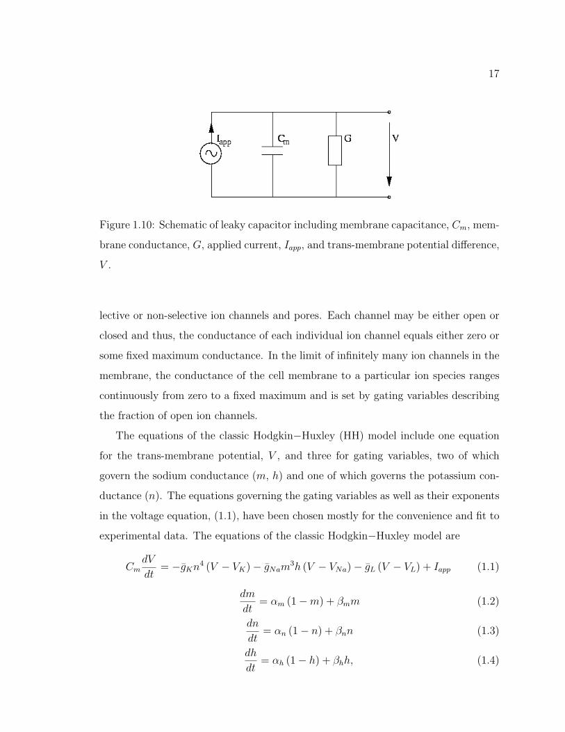
Figure 1.10: Schematic of leaky capacitor including membrane capacitance, Cm, mem-
brane conductance, G, applied current, Iapp, and trans-membrane potential difference,
V .
lective or non-selective ion channels and pores. Each channel may be either open or
closed and thus, the conductance of each individual ion channel equals either zero or
some fixed maximum conductance. In the limit of infinitely many ion channels in the
membrane, the conductance of the cell membrane to a particular ion species ranges
continuously from zero to a fixed maximum and is set by gating variables describing
the fraction of open ion channels.
The equations of the classic Hodgkin−Huxley (HH) model include one equation
for the trans-membrane potential, V , and three for gating variables, two of which
govern the sodium conductance (m, h) and one of which governs the potassium con-
ductance (n). The equations governing the gating variables as well as their exponents
in the voltage equation, (1.1), have been chosen mostly for the convenience and fit to
experimental data. The equations of the classic Hodgkin−Huxley model are
CmdV
dt= −gKn4 (V − VK)− gNam
3h (V − VNa)− gL (V − VL) + Iapp (1.1)
dm
dt= αm (1−m) + βmm (1.2)
dn
dt= αn (1− n) + βnn (1.3)
dh
dt= αh (1− h) + βhh, (1.4)
18
where αx and βx, for x ∈ m, n, h, are the following functions of v = V − V∞, the
difference of the trans-membrane potential from the resting potential:
αm = 0.1 25−v
exp( 25−v10 )−1
βm = 4exp(− v
18
)αn = 0.07exp
(− v
20
)βn = 1
exp( 30−v10 )+1
αh = 0.01 10−v
exp( 10−v10 )−1
βh = 0.125exp(− v
80
).
Defining the new functions x∞ and τx for x ∈ m, n, h according to
x∞ =αx
αx + βx
and τx =1
αx + βx
(1.5)
allows us to write the original gating equations, (1.2) through (1.4), in a more intuitive
form, namely (1.6) through (1.8), which demonstrates that each gating variable x ∈
m, n, h decays to its voltage dependent steady-state, x∞, with a voltage dependent
time constant, τx:
τm (v)dm
dt= m∞ (v)−m (1.6)
τn (v)dn
dt= n∞ (v)− n (1.7)
τh (v)dh
dt= h∞ (v)− h. (1.8)
The Slow-Fast Phase-Plane
To better understand the mechanism underlying the excitability and threshold be-
havior of the Hodgkin−Huxley model, we shall consider the slow-fast phase-plane
associated with (1.1) through (1.4).
Since the trans-membrane voltage is what we desire to understand and depends on
all fast and slow gating variables, it shall be the fast variable in the fast-slow phase-
plane. The dynamics of the gating variable m are much faster than the dynamics of
n or h. Thus, m is approximated by its voltage-dependent steady-state, m∞. The
dynamics of n and h occur on a slower time scale and, according to an observation
19
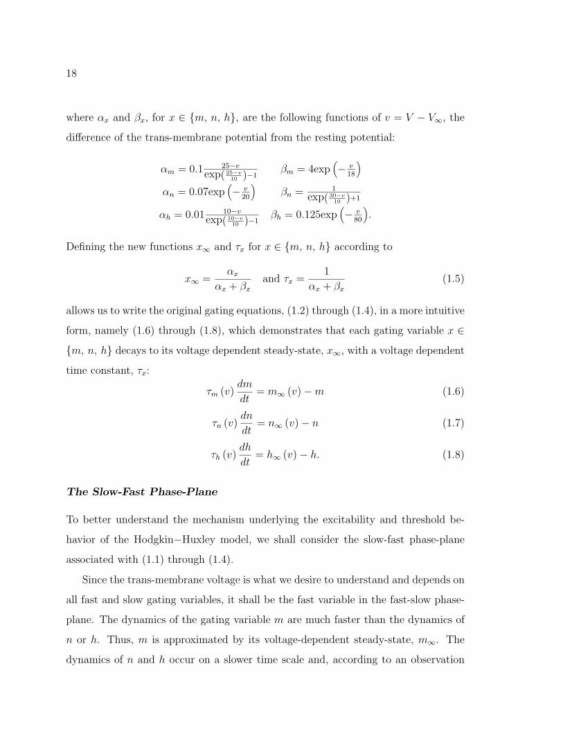
Figure 1.11: Nullclines and flow directions in the fast-slow phase-plane.
by FitzHugh, n + h ≈ 0.8. This allows us to eliminate h. The fast-slow variables are
V and n and satisfy
CmdV
dt= −gKn4 (V − VK)− gNam
3∞ (0.8− n) (V − VNa)− gL (V − VL) + Iapp (1.9)
dn
dt= αn (1− n) + βnn. (1.10)
Qualitatively, the nullcline on which dVdt
= 0 has the shape of a cubic in V and the
nullcline on which dndt
= 0 has the shape of a linear function. Figure 1.11 shows the
qualitative flow directions across the nullclines in the fast-slow phase-plane.
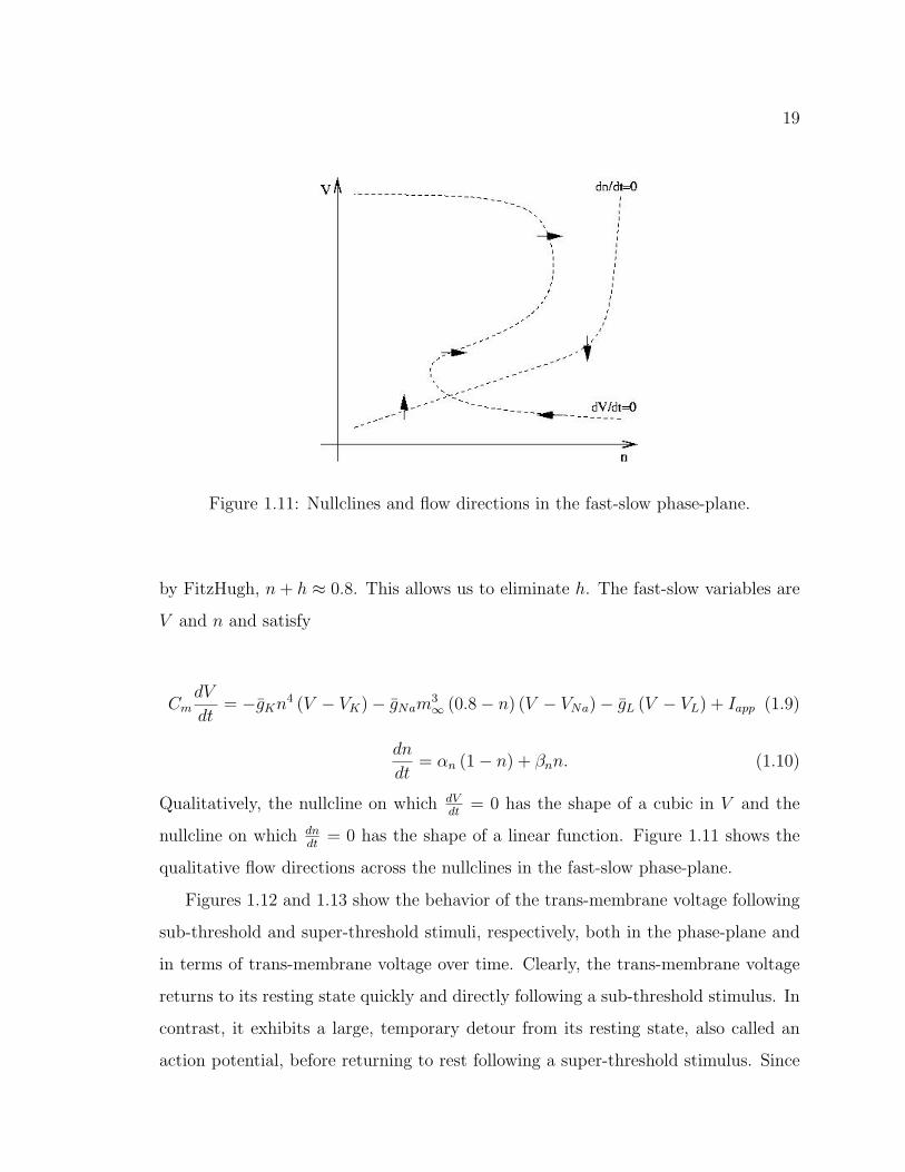
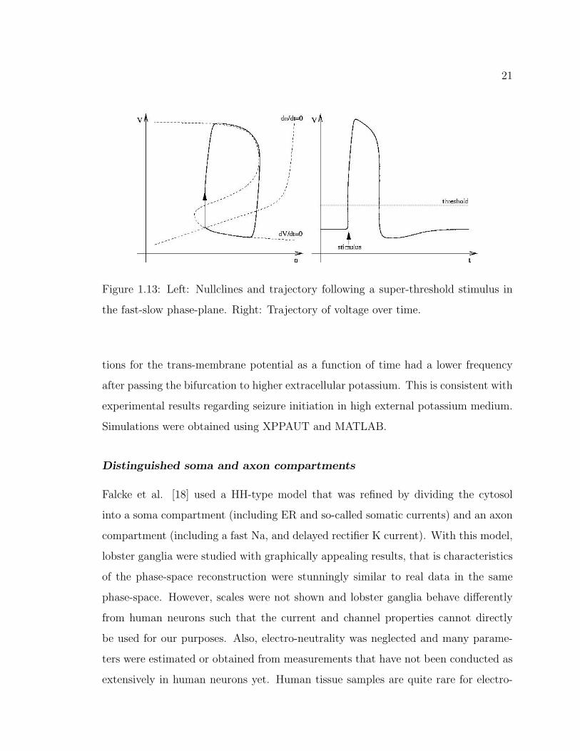
Figures 1.12 and 1.13 show the behavior of the trans-membrane voltage following
sub-threshold and super-threshold stimuli, respectively, both in the phase-plane and
in terms of trans-membrane voltage over time. Clearly, the trans-membrane voltage
returns to its resting state quickly and directly following a sub-threshold stimulus. In
contrast, it exhibits a large, temporary detour from its resting state, also called an
action potential, before returning to rest following a super-threshold stimulus. Since
20
Figure 1.12: Left: Nullclines and trajectory following a sub-threshold stimulus in the
fast-slow phase-plane. Right: Trajectory of voltage over time.
the dynamics of V are much faster than those of n, any motions in the V -direction
are much faster than those in the n-direction. As a result, any trajectory approaches
the nullcline on which dVdt
= 0 very quickly and spends most of its time close to it.
1.3.2 An Overview of Mathematical Neuron Models
HH-type double cycle burster
One particularly interesting HH-type model is the one by Shorten and Wall [73] based
on the work of Jacobsson [34, 54, 55] and LeBeau et al. [43, 44]. It exhibits bursting
behavior, in which the transition does not take place from a steady-state to a limit
cycle but between two different limit cycles. However, it does not include sodium or
chloride, which implies that it entirely neglects any treatment of electro-neutrality.
Furthermore, all extracellular concentrations are constant. Not shown here, a pre-
liminary numerical bifurcation study of the steady-states of the model with respect
to the external potassium concentration found a sub-critical (hard) Hopf bifurcation
within the physiologically relevant potassium range. Corresponding numerical solu-
21
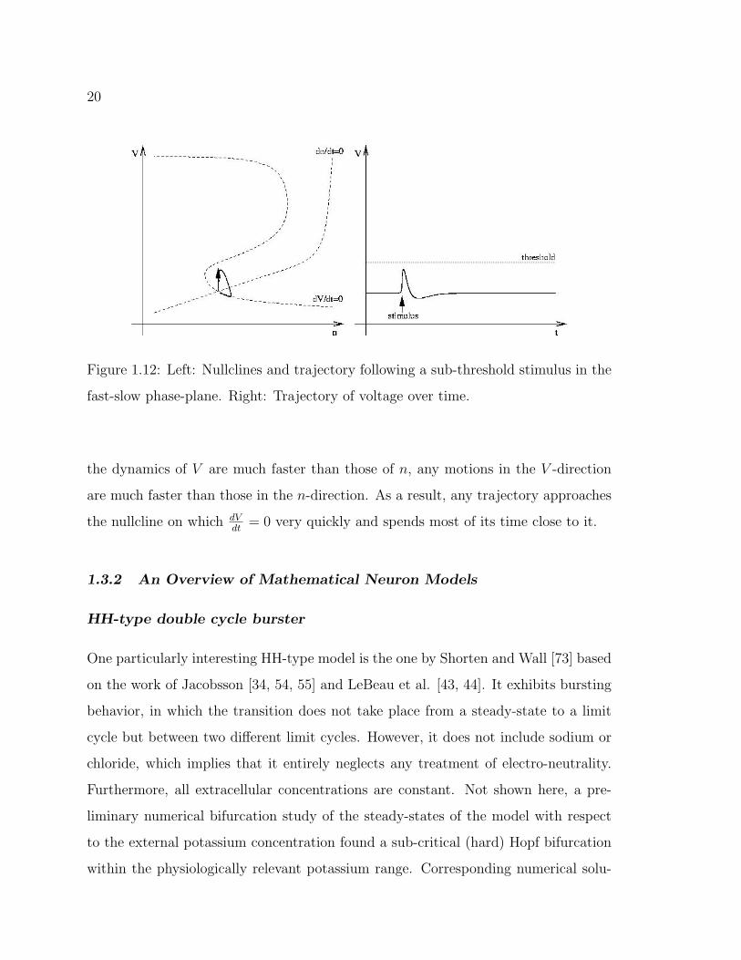
Figure 1.13: Left: Nullclines and trajectory following a super-threshold stimulus in
the fast-slow phase-plane. Right: Trajectory of voltage over time.
tions for the trans-membrane potential as a function of time had a lower frequency
after passing the bifurcation to higher extracellular potassium. This is consistent with
experimental results regarding seizure initiation in high external potassium medium.
Simulations were obtained using XPPAUT and MATLAB.
Distinguished soma and axon compartments
Falcke et al. [18] used a HH-type model that was refined by dividing the cytosol
into a soma compartment (including ER and so-called somatic currents) and an axon
compartment (including a fast Na, and delayed rectifier K current). With this model,
lobster ganglia were studied with graphically appealing results, that is characteristics
of the phase-space reconstruction were stunningly similar to real data in the same
phase-space. However, scales were not shown and lobster ganglia behave differently
from human neurons such that the current and channel properties cannot directly
be used for our purposes. Also, electro-neutrality was neglected and many parame-
ters were estimated or obtained from measurements that have not been conducted as
extensively in human neurons yet. Human tissue samples are quite rare for electro-
22
physiologists and thus, many of the relevant parameters from human tissue are not
known to date. Another possible reason for this lack of data is that those parame-
ters are no uniform properties of “human neuron” but instead take on a relatively
wide range of values within one kind of neuron as well as in different kinds of neurons
(personal correspondence with Dan Cook, Phil Schwartzkroin). Therefore, this model
cannot successfully be used for human neuron, at least at present.
Keener&Sneyd / Hoppensteadt&Peskin (KS/HP)
Consider a simple cell volume-control steady-state model: Na, K, and Cl are dis-
tributed by passive transport and only a Na-K pump is added for active transport.
Water flow due to osmotic pressure on the membrane is modeled using a mechanical
flow resistance of the membrane to water, the trans-membrane potential is related to
charges on the membrane, and ionic currents are governed by a set of Ohm’s laws with
linear current-voltage relations (chapter 2 in [36]). Further, trapped ions inside the
cell are taken into account in terms of their electric as well as osmotic effects. While
this dynamic formalism provides a correct picture of the membrane potential, we shall
see in section 4.5 that it, in its dynamic form, does not model ion transport accurately.
In the following, all dynamics are abandoned, the membrane charge (and in HP, [28],
but not in KS, [36], the direct osmotic effect of the trapped ions) is neglected, electro-
neutrality of interior and exterior compartments is imposed, and all fluxes are set to
zero. The steady-state volume of the cell is studied in relation to the pump rate and
the permeabilities of the membrane to K and Na. The HP/KS approach is purposely
kept simple and is designed to address the stability and qualitative dependence, but
not the dynamics, of the steady-state volume on model parameters. Thus, for its lack
of dynamics, this model is not suited to our goals as is. However, when modeling cell
volume dynamics, we may adopt a similar treatment of the osmotic forces that cause
the passage of water across the membrane.
23
Tracking net-charge versus tracking net-current
Work by Rudy et. al. [30] supports the view that maintaining electroneutrality in the
bulk is an important issue with current models for ion transport and trans-membrane
potential dynamics. The authors investigate whether long-term drifts occur when the
trans-membrane potential is determined from (a) the net-charge in the Debye layer
close to the membrane surface (“algebraic” method) or (b) a Hodgkin−Huxley-type
voltage equation that tracks the net-current across the membrane from an initial con-
dition onward (“differential” method). No difference between the dynamics produced
in both cases is found. The authors establish that long-term drifts in variables are,
among other possibilities, the result of a non-conservative implementation of stimuli.
When ions carried by the stimulus current are taken into account, the algebraic and
differential methods yield identical results. This is expected, since we show in subsec-
tion 4.2.1 for a system obeying mass-conservation that, with the use of appropriate
parameters, (a) and (b) are equivalent.
Debye layer distinguished from bulk space
Yet another approach has been taken by Genet & Costalat [21]. They used results
of Grahame [23], who conducted a theoretical study of the electrostatic properties of
the double layer (Debye layer) near the cell membrane for a circular cell bathed in
an infinite medium. Based on Grahame’s work, they developed a model analogous
to the one of Jacobsson [34], except for the addition of Boltzmann dynamics between
the bulk and the region close to the membrane on either side of a charged membrane.
The transition of ions across the membrane is assumed to only take place from one
part of the electric double layer to the other and to be much slower than the transition
of water across the membrane. The membrane is assumed to bear a fixed amount of
surface charges, which implies a direct relation of membrane surface charge density
and cell volume. However, a correct representation of the trans-membrane potential
24
based on present ion concentrations is neglected entirely. Using this model, the effects
of membrane surface charges onto the electro-osmotic regulation in the cell are inves-
tigated. Besides defining a relation of external Ca and Na pump rates, the study also
finds the steady-state more stable and supporting a larger cell volume in the presence
of surface charges accumulated at a charged membrane, compared to the case of an
uncharged membrane.
Numerical study of neural connectivity
In simulations of huge neuron populations, an external concentration may be used as
a coupling variable. The main interest of such studies tends to lie not in the electro-
physiologically consistent modeling of a single neuron within a population but instead
in the qualitative influence of coupling parameters between different groups of neuron
populations onto their own activity and onto its spread through the population. Such
simulations are too complicated for analytical treatment or study, do not seek electro-
physiological consistency, and shall thus not be considered here. (see, e.g., [42]).
Diffusion-type PDE model of spreading depression
Spreading depression consists of slowly moving waves of membrane depolarization and
prolonged depression of EEG activity in the brain and is accompanied by ionic con-
centration changes lasting up to two minutes. It is widely believed to cause migraine-
with-aura. Since many of the same processes are involved on a cellular level, spreading
depression can be considered related to epilepsy in that sense. In terms of the obser-
vations in EEG, one might think of the two as opposites. Shapiro [70] developed a
computational model for the spread of depression waves in neural tissue based on a
macroscopic electro-diffusion equation that incorporates the effects of gap junctions
and osmotic forces. As a PDE model, it also incorporates intracellular voltage and
concentration gradients. Bulk electro-neutrality is assumed and the volume at each
time step is set to its steady-state value in simulations. This model does not seek
25
electro-physiological consistency and is too complex for the analytic study of relations
between its parameters or variables.
Stefan problem for ion transport across elastic membrane
This approach of Rubinstein & Geiman [20, 65] only considers passive transport of
non-electrolytes across a deformable, semi-permeable membrane. Its curvature is as-
sumed to influence the thickness of the membrane, and the derived equations are
applied to the swelling of muscle fiber. First, a plane-parallel model of the fiber is
studied and then a cylindrical one. Assuming a preferred direction of flow, the model
reduces to one dimension. In another approach, called the “pure diffusion approxima-
tion” by the authors, all convective terms due to strong discontinuities are neglected
and so is the diffusion flux induced by the moving boundary itself. This model fo-
cuses on the interactions between the deformable membrane and the transport across
it and thus lacks electrically charged particles and their active transport across the
membrane, properties critical to our approach.
1.4 Limitations of Current Models in Tissue Modeling
Hodgkin−Huxley-type models have been used to successfully model individual neu-
rons, groups of neurons, as well as the interactions between multiple groups of neurons.
As relative computing times decrease, efficient simulations of mathematical models
become more detailed and, as such, more powerful in their quantitative accuracy of
predictions. This has made mathematical simulations an attractive, non-invasive, and
relatively cheap tool in assisting the formulation of hypotheses, the prediction of their
accuracy, and thus the design of experiments that ultimately test those hypotheses.
In contrast to expensive and invasive animal models, a natural extension to current
neuron models is thus enabling them to model a cell within its natural, resident,
and live tissue with quantitative accuracy. Cells in tissue are closely surrounded by
26
other cells, sharing with them a relatively small external environment. Under certain
conditions, the ion concentrations in the external environment as well as the external
volume fraction can undergo relatively large temporal detours from their normal val-
ues. Therefore, a suitable model for cells in tissue may not assume a cell with fixed
volume immersed in a constant environment, as is the case for Hodgkin−Huxley-type
models. An extended mathematical model including the features of dynamic external
concentrations and cell volume will contribute to the better understanding of cells in
tissue and is not restricted to neural tissue in its applicability.
Considering finite internal and external media for an individual cell and its imme-
diate environment leads to the question of mass conservation and, more importantly,
electro-neutrality. In many approaches using fixed interstitial concentrations, electro-
neutrality is either neglected entirely or enforced externally, as described in 1.3.2.
However, neither is appropriate when working with a finite medium.
1.4.1 Reflection on Problems with Current Models
As pointed out previously, most of the models briefly described in 1.3.2 do not con-
sider a variable volume or variable external concentrations. The Keener and Sneyd
approach [36] is purposely kept simple and is designed to address the stability and
qualitative dependence, but not the dynamics, of the steady-state volume on the pump
rate and membrane permeabilities. In this model of cell volume-control and ionic dy-
namics, the full equations give an equilibrium distribution of various ions in the two
compartments without satisfying electro-neutrality. In other words, the stationary
solution is inconsistent with the Donnan equilibrium for bulk ionic concentrations.
This problem stems from the existence of a boundary layer, also known as electric
double layer or Debye layer, in which the electro-neutrality condition is not valid.
Outside this layer, in the bulk, it can be shown that electro-neutrality is rigorously
met, consistent with the fact that separating a pair of charges into a macroscopic
distance is energetically impossible in the given setting. Hence, while the expression
27
for the trans-membrane potential in this model is valid for the double layer, it is
not valid for the bulk, where another equation has to be introduced. More precisely,
the net charges on either side of the membrane are both extremely small but their
difference cannot be neglected in the double layer. Nevertheless, electro-neutrality is
enforced in Keener and Sneyd’s model without setting the trans-membrane potential
to zero, which should be the first consequence of this approximation. A by-product
of this discrepancy is that, after the dynamic model is reduced to a static model,
no one trans-membrane potential can be found that satisfies all their equations for
physiologically reasonable parameter values. The condition needed to obtain a con-
sistent result is to set the charges on the present impermeant ions to zero, causing
the loss of the electrical effect of these molecules. However, even then, the trans-
membrane potential equals zero only if the pump rate equals zero. This is a major
difficulty of this formalism, since at this point electro-neutrality contradicts its valid-
ity in the non-electro-neutral double layer. Further, a constant, zero trans-membrane
potential indicates that the steady-state corresponding to a dead cell is being investi-
gated, which is not the steady-state supported by the full, dynamic model equations.
Thus, this model cannot be used if one is interested in the accurate, inter-dependent,
dynamic description of the cell volume and trans-membrane potential.
The model of Genet & Costalat [21] is also mostly interested in the steady-state
and uses an inadequate relation of ion concentrations and trans-membrane potential.
Furthermore, due to Grahame’s theory [23], it is valid for a spherical cell, which is
rather different from the appearance of neurons. Shapiro’s model [70] is a compu-
tational model that does not allow analytical treatment and, finally, Rubinstein’s
model [20, 65] does not consider the exchange of electrolytes across the membrane
and neglects any convective terms. This implies that the solution does not exhibit a
boundary layer. Especially this latter simplification cannot be upheld in an accurate,
electro-diffusion type setting. In general, in some of the described models, chloride
is used to maintain electro-neutrality in the bulk, whereas others do not include any
28
anion species and hence totally neglect the question of electro-neutrality. This seems
contradictory since, from an energetic point of view, it is impossible to separate a
pair of charges in the given setting.
Intuition says that there must be a fundamental difference between assuming
electro-neutrality or not doing so and that this is clearly a discrepancy which should
be pursued and understood. In pursuit of the fundamental question about the reason-
ableness of the assumption of electro-neutrality, the expected result is that either one
of these two approaches is found fundamentally wrong, or both of them are related
in a way to be characterized.
1.5 Toward Biophysically Consistent Tissue Modeling
Modeling a cell in tissue requires one to accurately model charge-carrier transport
between two compartments with finite volume. Here, accuracy is to be understood
in the sense of biophysical consistency and implies, for example, that charges cannot
accumulate in free solution. Instead of improving an existing model in a heuristic
way by, for example, forcing the existing Hodgkin−Huxley model to maintain electro-
neutrality in bulk solution, I pursue a more theoretical approach by seeking to develop
a model, based on the fundamental physical chemistry of ion movement, that naturally
captures the characteristics of charge-carrier transport.
To achieve this goal, I investigate the problem of bulk electro-neutrality during pas-
sive charge-carrier transport in a self-imposed electric field across a thin, lipid mem-
brane. Under assumptions of uniformity and homogeneity, this process is described
mathematically by an electro-diffusion system in 1D, a highly nonlinear system of par-
tial differential equations (PDEs). An explicit solution for the electro-diffusion system
does not exist and, even though it is a well-defined problem in applied mathematics,
computing its solutions numerically is not trivial, either.
In the course of this dissertation, three consecutive approximations of the 1D
29
electro-diffusion system are developed: The first, formal, mathematical approximation
is a quasi steady-state approximation (QSSA) and constitutes the most fundamental
model of electro-diffusion. It is based solely on the relative sizes of physical parameters
of the system. The second, constant field approximation (CFA) of the electro-diffusion
system applies a GHK-like constant field assumption to the QSSA and thus constitutes
a more physical model of electro-diffusion. A constant electric field throughout the
membrane region of the domain implies that the membrane region is locally electro-
neutral, while any local net charge accumulates at its boundaries. The CFA is most
fundamentally different from the classic HH-GHK model found in literature in that
it incorporates conditions of mass conservation and is derived mathematically from
an electro-diffusion system. The third, Hodgkin−Huxley pump-leak approximation
(HH-plk) of the electro-diffusion system is a linearization of the QSSA with respect
to the trans-membrane potential that contains HH-type ohmic fluxes. This simplest
model of electro-diffusion is equivalent to a combination of (a) a HH model for the
trans-membrane potential with (b) a so-called pump-leak model for the concentration
dynamics and (c) conditions of mass conservation. Previous approaches have resulted
in models similar to this one but none of them has incorporated all the aspects
required for our problem. In addition, our analysis provides a concrete, mathematical
justification for the HH-plk model.
In chapter 2, analytic work on the electro-diffusion system is presented: The setup
and assumptions for the 1D electro-diffusion system are introduced, the formal quasi
steady-state approximation (QSSA) is developed, and a relaxation time to equilibrium
derived. Also, analytic equilibrium solutions are computed for systems containing
various combinations of valencies. In chapter 3, the validity of the QSSA is demon-
strated numerically: I discuss the numerical method chosen to simulate the transient
dynamics of the electro-diffusion system and develop an almost-Newton, iterative
method to solve for the steady-state of the electro-diffusion system. The QSSA is
implemented by incorporating the almost-Newton steady-state solver into a dynamic
30
updating scheme. Results of the QSSA are compared to the fully transient approach
of the electro-diffusion system to Donnan equilibrium for three sets of initial condi-
tions. In chapter 4, the QSSA is connected with the classic Hodgkin−Huxley theory:
The models resulting from the constant field approximation (CFA) and linearization
(HH-plk) of the QSSA are introduced and compared to the QSSA in the case of a
dying cell. CFA and HH-plk are then compared to the classic Hodgkin−Huxley model
in case of a living cell. Chapter 5 contains a summary and discussion of results and
an outlook toward future work motivated by those results.
It would be nice if, for completeness, the QSSA could be compared to the classic
Hodgkin−Huxley model in the case of a living cell. This would require the presence
of active ion transport to maintain homeostasis, and thus the incorporation of source
terms into the steady-state solver. See section B.2 for the derivation of equations
for a modified, almost-Newton steady-state solver that includes source terms from
space-dependent but concentration-independent sources. Solving the semiconductor-
device equations, that is the Poisson−Nernst−Planck system in the presence of highly
nonlinear source terms, has caused problems with stiffness as reported, for example,
by Ringhofer and Korman [62, 39]. Thus, the convergence of my modified method
may be expected to be stiff, especially if the source terms represent point sources. It
may therefore not provide an efficient means of simulating its corresponding, modified
quasi steady-state approximation. Obtaining results from the modified steady-state
solver is not essential to our conclusions and shall thus be left as a future challenge.
This dissertation demonstrates that the QSSA provides the most rigorous and
most accurate model of electro-diffusion and that, in its current state, the QSSA
lacks efficiency and the ability to incorporate active ion transport, which are essential
to simulating the living state of a cell. The CFA provides a reasonably accurate model
of electro-diffusion in the sense that it provides good approximations of flux densities
and trans-membrane potential and, most importantly, in that it self-regulates bulk
electro-neutrality. It is also capable of efficiently incorporating active ion transport
31
and thus of simulating the living state of a cell. The HH-plk model provides a good
approximation of the trans-membrane potential and is capable of efficiently simulating
the living state of a cell. However, it does not match flux densities closely and thus
does not self-regulate bulk electro-neutrality very well. Therefore, the CFA emerges as
an efficient and accurate means of modeling the ion transport and potential difference
across lipid membranes that separate two finite compartments from each other.

32
Chapter 2
ION TRANSPORT BY ELECTRO-DIFFUSION
Ion transport has been modeled in various media and on various scales of size
using different mathematical approaches. One of the most fundamental continuum
models for the motion of charged particles, or rather the time evolution of particle
density distributions, is a nonlinear system of partial differential equations (PDEs)
often called the electro-diffusion system. These equations describe particle diffusion
in a particle-created electrostatic field and consist of an electro-diffusion equation
for each particle-type in the system and a single, coupling Poisson equation for the
electrostatic field.
The best understood phenomenon in this context is probably the classic Donnan
equilibrium. The principle of Donnan exclusion arises in many physical, chemical,
and biological systems involving electrically charged particles [10]. Its applications
span semiconductors, colloid-chemistry, nanofiltration, ion-exchange membranes, and
the pulp and paper industry to name just a few. The Donnan equilibrium is estab-
lished in a closed system of ionic species with a semi-permeable membrane separating
two compartments from each other. At least one ionic species is impermeant to
the membrane. The elementary theory to compute the equilibrium concentrations
in and the electrical potential difference between the compartments assumes electro-
neutrality in each compartment and salt equilibrium of the permeant species [16]. A
more accurate, rigorous theory for Donnan equilibrium considers a system of electro-
diffusion and Poisson equations for particle concentrations and electrostatic poten-
tial, respectively, whose equilibrium solution yields the Donnan equilibrium [64, 22].
Alternatively, the equilibrium of the PDE system can be described by a single, time-
33
independent equation for the electrostatic potential. This equation is also known as
the Poisson−Boltzmann equation and has found many applications in molecular bi-
ology in recent years [27]. For a large class of applications with realistic geometric
settings, the equilibrium solution is nearly constant in each of the compartments but
exhibits a thin boundary layer near the location of the membrane with a sharp tran-
sition of variables from their internal to their external values. The solutions far away
from the boundary layer are consistent with the classic Donnan equilibrium [64].
The electro-diffusion equations shall be investigated in detail in the following sec-
tions. In particular, simplifying assumptions are discussed that allow the application
of these equations to ion transport across thin, lipid membranes. Furthermore, ap-
propriate boundary conditions are discussed for the time-dependent PDE model, the
steady-state problem, and equilibrium. Because of the complexity of the system, ex-
plicit, analytic solutions are neither available for the transient equations nor for the
steady-state problem. However, an estimate for the exponential time-scale for the ap-
proach of the system to Donnan equilibrium is determined in section 2.2 and analytic
equilibrium solutions are derived in section 2.3 for cases in which the largest valency
is ±2.
2.1 Setup and Assumptions for Simulating Electro-Diffusion
and Poisson Equations
This section attempts to give an overview of the issues involved and approaches taken
in numerically simulating the fully transient electro-diffusion system. For a detailed
treatment of the numerics see section 3.1. The electro-diffusion equations describing
particle diffusion in a particle-created electrostatic field, also called the semiconductor-
device equations, are, in their most general form,
∂ci
∂t= ∇ · [Di (∇ci + zi∇ϕ ci) + Si] (2.1)
34
∇ · (ε∇ϕ) +∑
i
zici = −N, (2.2)
where subscripts i indicate that a quantity is specific to ionic species i, concentrations
are denoted by c, diffusion coefficients by D, valencies by z, source terms by S, and
fixed space-charges within the medium by N . ϕ is the normalized, electrostatic poten-
tial and ε a small, non-dimensional quantity proportional to the dielectric coefficient
of the medium. In particular,
ϕ = − FV
R0Tand (2.3)
ε =ε0εrR0T
δ2c F 2, (2.4)
where V is absolute voltage, F is Faraday’s constant, R0 is the universal gas constant,
T is absolute temperature, ε0 is the dielectric in vacuum, εr > 1 is the relative
dielectric coefficient, c is a characteristic concentration, and δ a characteristic length
scale of the system. We will subsequently refer to ε as the dielectric coefficient. Note
that valencies, z, are integer and that the diffusion and dielectric coefficients, D and
ε, are generally space dependent.
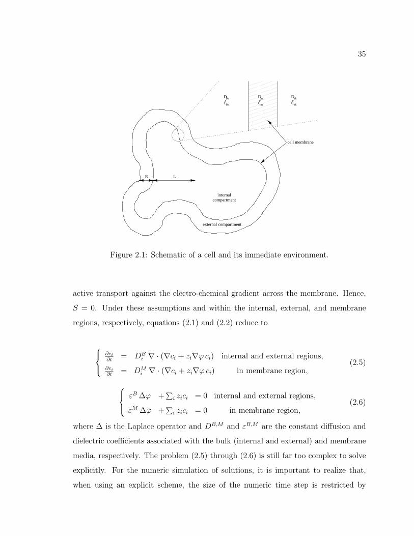
To introduce simplifying assumptions that make sense in the case of ion trans-
port across thin, lipid membranes, consider figure 2.1, showing a schematic of a cell
and its immediate environment. The characteristic length scales, L and R, of the
internal and external space are large compared to the finite width of the membrane
separating the compartments. As a first approximation and for lack of otherwise
detailed information, it certainly makes sense to assume that the internal, external,
and membrane spaces are filled with uniform, homogeneous material. As a result, the
diffusion and dielectric coefficients, D and ε, are piecewise constant. We shall further
assume that the internal, external, and membrane media are neutral, that is they
contain the charged ionic particles governed by (2.1) but do not contain any fixed
space charges. Thus, N = 0. Investigating the passive transport of ions across the
lipid membrane, we shall further neglect any source terms due to chemical reactions or
35
D D D
m
m bk
bk
bk
bk
external compartment
R L
internal compartment
cell membrane
Figure 2.1: Schematic of a cell and its immediate environment.
active transport against the electro-chemical gradient across the membrane. Hence,
S = 0. Under these assumptions and within the internal, external, and membrane
regions, respectively, equations (2.1) and (2.2) reduce to
∂ci
∂t= DB
i ∇ · (∇ci + zi∇ϕ ci) internal and external regions,
∂ci
∂t= DM
i ∇ · (∇ci + zi∇ϕ ci) in membrane region,(2.5)
εB ∆ϕ +∑
i zici = 0 internal and external regions,
εM ∆ϕ +∑
i zici = 0 in membrane region,(2.6)
where ∆ is the Laplace operator and DB,M and εB,M are the constant diffusion and
dielectric coefficients associated with the bulk (internal and external) and membrane
media, respectively. The problem (2.5) through (2.6) is still far too complex to solve
explicitly. For the numeric simulation of solutions, it is important to realize that,
when using an explicit scheme, the size of the numeric time step is restricted by
36
∆t ≤ ∆x2
max(D), a quantity that is proportional to the inverse of the largest diffusion
coefficient in the problem (see section 3.1). The diffusion coefficients in the internal
and external bulk regions are, in fact, about three orders of magnitude larger than
the diffusion coefficients in the membrane region and thus, the problem is much more
time intensive to solve in the bulk regions. On the other hand side, our interest
lies not so much in the fast dynamics of ion species in the bulk regions but much
rather in the relatively slow dynamics of ion species crossing the membrane region
from one bulk region into the other. In order to compute numeric solutions within
a reasonable time-frame, we shall approximate both, the internal and external, bulk
compartments as well mixed and equilibrated within themselves on the time scale on
which the dynamics of ionic species passing the membrane region are observed. As a
result, the internal and external bulk concentrations are constant and we may focus
on the dynamics in the membrane region. We shall see in subsection 2.1.1 that this
assumption requires a careful choice of remaining conditions. Assuming further that
the membrane has a uniform width, say m, allows us to consider the problem in 1D
and focus on the membrane region. Equations (2.5) through (2.6) reduce to
∂ci
∂t= Di
∂
∂x
(∂ci
∂x+ zi
∂ϕ
∂xci
)(2.7)
ε∂2ϕ
∂x2+∑
i
zici = 0 (2.8)
for x ∈[−m
2; m
2
], where D and ε are the diffusion and dielectric coefficients associ-
ated with the membrane medium. The bulk concentrations, c (−L) and c (R), are
the boundary conditions for (2.7) and are updated via ordinary differential equations
involving the compartment volumes and flux densities across the membrane bound-
aries at ±m2. The latter ensures zero-flux out of the system boundaries and thus mass
conservation and charge conservation in the entire system.
37
2.1.1 Flux Conditions for Impermeant Species
In addition to zero-flux conditions at the system boundaries, zero-flux conditions also
need to be met within the domain by any ion species impermeant to the membrane.
At any location within the domain at which zero flux is enforced for some species there
forms a Debye layer. Each side of this double boundary layer is of order O (√
ε), and
in it local electro-neutrality is not met. Instead, a non-zero concentration gradient
and electrostatic potential gradient coexist. Zero-flux conditions at both ends of the
membrane, x = −m2
and x = m2, are the obvious physical conditions and give rise
to a Debye layer with one side of each double layer in a bulk region. Thus, ion
concentrations are not constant in a thin part of the bulk region, which contradicts
my previous assumption that ion concentrations are constant throughout the bulk. In
section 4.1, where zero-flux conditions at both ends of the membrane are used, the bulk
concentrations away from the Debye layer are approximated by their average values
throughout the internal or external compartments. These average values include the
average over each Debye layer and are appropriate to use there, considering that the
size of each Debye layer is much less than the size of the bulk compartment.
When simulating the fully transient electro-diffusion system, using average values
is not approriate. Thus, to save computation time and comply with constant bulk
concentrations here, we need a single zero-flux condition at mid-membrane, x = 0. In
this case, the Debye double layer lies to either side of the location x = 0 within the
membrane. Bulk concentrations are constant and locally electro-neutral, consistent
with the previous assumption and provided that half the width of the membrane is
less than the width of the boundary layer, m2≤√
ε. For convenience, we shall assume
in the following that m2
=√
ε. In other words, the mathematical boundary layer is
filled with membrane medium. For appropriate parameter values, this results in a
membrane width of about 26 to 76 A, about 0.5 to 1.5 times the width of a biological
cell membrane. In particular, the width of the double boundary layer is
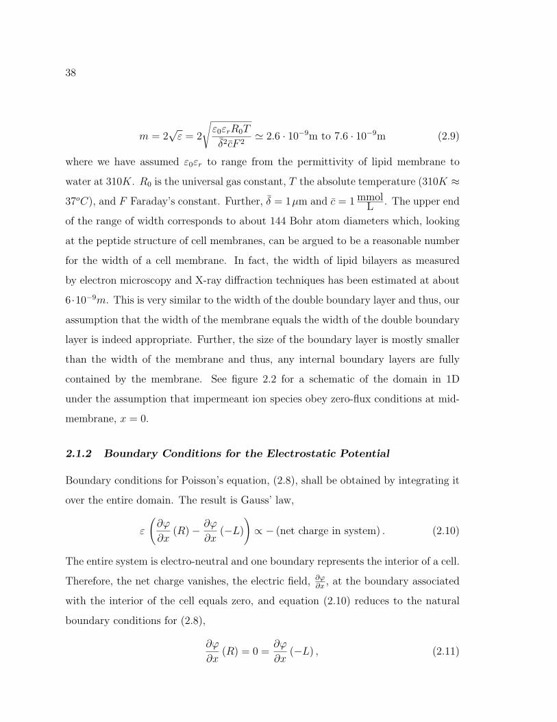
38
m = 2√
ε = 2
√ε0εrR0T
δ2cF 2' 2.6 · 10−9m to 7.6 · 10−9m (2.9)
where we have assumed ε0εr to range from the permittivity of lipid membrane to
water at 310K. R0 is the universal gas constant, T the absolute temperature (310K ≈
37oC), and F Faraday’s constant. Further, δ = 1µm and c = 1 mmolL . The upper end
of the range of width corresponds to about 144 Bohr atom diameters which, looking
at the peptide structure of cell membranes, can be argued to be a reasonable number
for the width of a cell membrane. In fact, the width of lipid bilayers as measured
by electron microscopy and X-ray diffraction techniques has been estimated at about
6 ·10−9m. This is very similar to the width of the double boundary layer and thus, our
assumption that the width of the membrane equals the width of the double boundary
layer is indeed appropriate. Further, the size of the boundary layer is mostly smaller
than the width of the membrane and thus, any internal boundary layers are fully
contained by the membrane. See figure 2.2 for a schematic of the domain in 1D
under the assumption that impermeant ion species obey zero-flux conditions at mid-
membrane, x = 0.
2.1.2 Boundary Conditions for the Electrostatic Potential
Boundary conditions for Poisson’s equation, (2.8), shall be obtained by integrating it
over the entire domain. The result is Gauss’ law,
ε
(∂ϕ
∂x(R)− ∂ϕ
∂x(−L)
)∝ − (net charge in system) . (2.10)
The entire system is electro-neutral and one boundary represents the interior of a cell.
Therefore, the net charge vanishes, the electric field, ∂ϕ∂x
, at the boundary associated
with the interior of the cell equals zero, and equation (2.10) reduces to the natural
boundary conditions for (2.8),
∂ϕ
∂x(R) = 0 =
∂ϕ
∂x(−L) , (2.11)
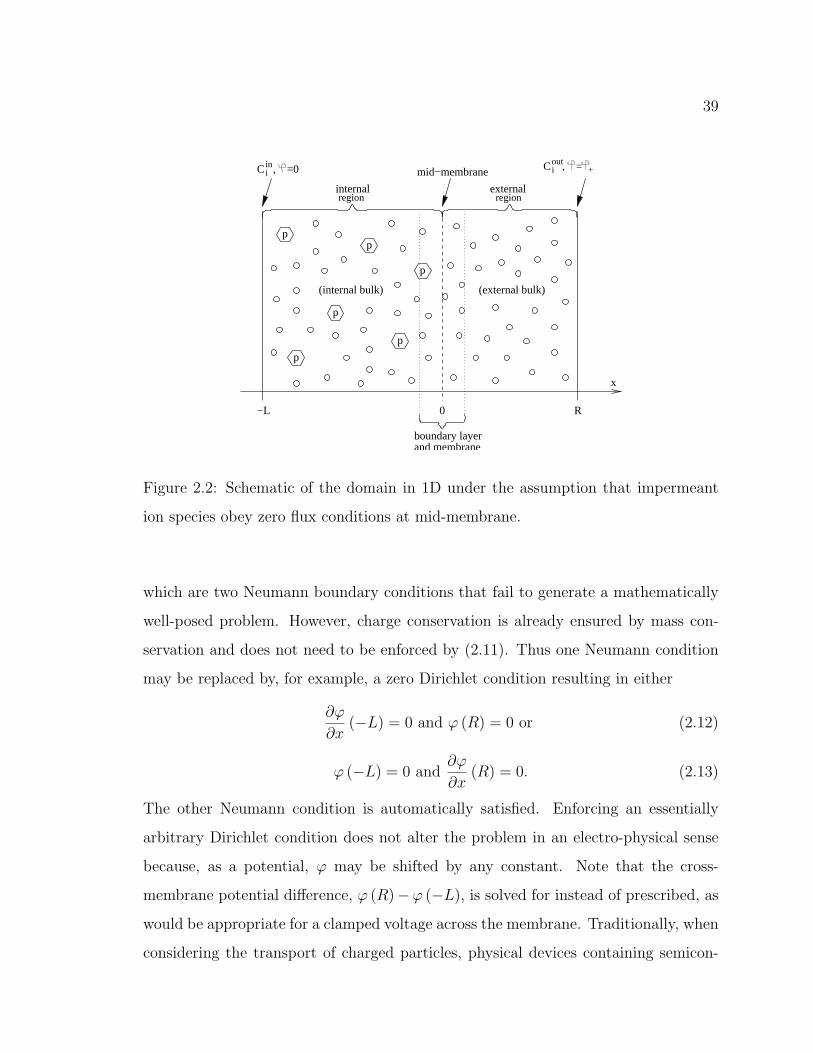
39
and membrane
region region
−L 0 R
x
p
p
p
p
p
p
C , =0iin C , =i
out+mid−membrane
boundary layer
(internal bulk) (external bulk)
internal external
Figure 2.2: Schematic of the domain in 1D under the assumption that impermeant
ion species obey zero flux conditions at mid-membrane.
which are two Neumann boundary conditions that fail to generate a mathematically
well-posed problem. However, charge conservation is already ensured by mass con-
servation and does not need to be enforced by (2.11). Thus one Neumann condition
may be replaced by, for example, a zero Dirichlet condition resulting in either
∂ϕ
∂x(−L) = 0 and ϕ (R) = 0 or (2.12)
ϕ (−L) = 0 and∂ϕ
∂x(R) = 0. (2.13)
The other Neumann condition is automatically satisfied. Enforcing an essentially
arbitrary Dirichlet condition does not alter the problem in an electro-physical sense
because, as a potential, ϕ may be shifted by any constant. Note that the cross-
membrane potential difference, ϕ (R)−ϕ (−L), is solved for instead of prescribed, as
would be appropriate for a clamped voltage across the membrane. Traditionally, when
considering the transport of charged particles, physical devices containing semicon-
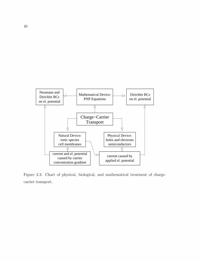
40
Mathematical Device:PNP Equations
Dirichlet BCson el. potential
Neumann andDirichlet BCson el. potential
Charge−CarrierTransport
Physical Device:holes and electrons
semiconductors
Natural Device:ionic species
cell membranes
current and el. potentialcaused by carrier
concentration gradient applied el. potentialcurrent caused by
Figure 2.3: Chart of physical, biological, and mathematical treatment of charge-
carrier transport.
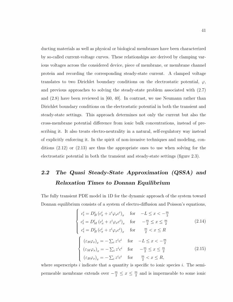
41
ducting materials as well as physical or biological membranes have been characterized
by so-called current-voltage curves. These relationships are derived by clamping var-
ious voltages across the considered device, piece of membrane, or membrane channel
protein and recording the corresponding steady-state current. A clamped voltage
translates to two Dirichlet boundary conditions on the electrostatic potential, ϕ,
and previous approaches to solving the steady-state problem associated with (2.7)
and (2.8) have been reviewed in [60, 40]. In contrast, we use Neumann rather than
Dirichlet boundary conditions on the electrostatic potential in both the transient and
steady-state settings. This approach determines not only the current but also the
cross-membrane potential difference from ionic bulk concentrations, instead of pre-
scribing it. It also treats electro-neutrality in a natural, self-regulatory way instead
of explicitly enforcing it. In the spirit of non-invasive techniques and modeling, con-
ditions (2.12) or (2.13) are thus the appropriate ones to use when solving for the
electrostatic potential in both the transient and steady-state settings (figure 2.3).
2.2 The Quasi Steady-State Approximation (QSSA) and
Relaxation Times to Donnan Equilibrium
The fully transient PDE model in 1D for the dynamic approach of the system toward
Donnan equilibrium consists of a system of electro-diffusion and Poisson’s equations,cit = Di
B (cix + ziϕxc
i)x for −L ≤ x < −m2
cit = Di
M (cix + ziϕxc
i)x for −m2≤ x ≤ m
2
cit = Di
B (cix + ziϕxc
i)x for m2
< x ≤ R
(2.14)
(εBϕx)x = −∑i z
ici for −L ≤ x < −m2
(εMϕx)x = −∑i zici for −m
2≤ x ≤ m
2
(εBϕx)x = −∑i zici for m
2< x ≤ R,
(2.15)
where superscripts i indicate that a quantity is specific to ionic species i. The semi-
permeable membrane extends over −m2≤ x ≤ m
2and is impermeable to some ionic

42
species at its midpoint, x = 0. We denote concentrations by c, diffusion coefficients
by DB in bulk solution and by DM in membrane, valencies by z, and the normalized,
electrostatic potential by ϕ. It is understood that the natural length scales of each
compartment are R− m2
= vout
Aand L− m
2= vin
A, where vin,out denote the volumes of
the compartments and A is the surface area of the semi-permeable membrane.
The uniqueness of the solution to this system of PDEs has been investigated in the
past. Rubinstein [63] discovered that, by enforcing local electro-neutrality, there are
multiple steady-states to the problem. However, recent studies have shown that, with-
out the artificial enforcement of local electro-neutrality, there is a unique steady-state
corresponding to any potential difference across the semi-permeable membrane [57, 9].
In a comparison between the cable equation and a Poisson−Nernst−Planck (PNP)
model, Leonetti [46] also concluded that the assumption of local electro-neutrality is
not suitable for studying the electric behavior of biological membranes. He demon-
strates this in the “negative differential conductance” regime and further develops
his bio-membrane electro-diffusive model based on PNP in terms of a set of jump
conditions for the electric field across dielectric material boundaries. The model is
concerned with the spatial propagation of action potentials in an excitable membrane
and does not address ion transport across membranes based upon PNP.
This section is structured as follows: Based upon the assumption that maxi (DiM)
mini (DiB), in subsection 2.2.1 we establish that the concentrations in bulk solution
are spatially constant to leading order. In subsection 2.2.2, we derive ODEs govern-
ing the dynamics of bulk concentrations. Under the assumption that m2 R ≤ L,
we establish that, to leading order, the membrane region is at steady-state. At this
point, we have reached a quasi steady-state approximation (QSSA) of the original
PDE system. We state the equations defining this QSSA in subsection 2.2.3. We fur-
ther analytically determine a relaxation time and demonstrate that it yields a good
approximation of the dynamic approach to Donnan equilibrium. The analytic expres-
sion for the relaxation time provides an explicit, testable, a priori prediction based

43
solely on physical parameters of the system.
2.2.1 Spatially Constant Bulk Concentrations
We assume in the following that maxi (DiM) mini (D
iB). Rescaling space by x = 2x
m
and time by t =(
2m
)2Dmin
M t, where DminM = mini (D
iM), we obtain
σi
Bcit = (ci
x + ziϕxci)x for −2L
m≤ x < −1
σiMci
t = (cix + ziϕxc
i)x for −1 ≤ x ≤ 1
σiBci
t = (cix + ziϕxc
i)x for 1 < x ≤ 2Rm
,
(2.16)
in which σiM =
DminM
DiM
= O (1) and σiB =
DminM
DiB 1. This clearly indicates the presence
of two different time scales in the bulk and membrane regions of the domain. To
observe the relatively slower time scales, we may, as a first approximation, neglect
the small terms σiBci
t and approximate the dynamics by0 = (ci
x + ziϕxci)x for −2L
m≤ x < −1
σiMci
t = (cix + ziϕxc
i)x for −1 ≤ x ≤ 1
0 = (cix + ziϕxc
i)x for 1 < x ≤ 2Rm
,
(2.17)
which implies in turn thatci (t, x) = ci
in for −2Lm≤ x < −1
σiMci
t = (cix + ziϕxc
i)x for −1 ≤ x ≤ 1
ci (t, x) = ciout for 1 < x ≤ 2R
m.
(2.18)
Thus, the dynamics in t, as shown in (2.18), describe the relaxation of the membrane
region to the steady-state associated with the current bulk concentrations, ciin,out.
2.2.2 Membrane Region at Steady-State
Since bulk concentrations are at steady state on the time scale on which t changes,
we expect them to change with respect to a relatively slower time scale. To obtain
44
dynamics for the bulk concentrations, we track the total mass by integrating over
each bulk compartment,
d
dt
∫ −1
− 2Lm
ci (t, x) dx =(
2L
m− 1
)dci
in
dt=
1
σiM
(cix + ziϕxc
i)∣∣∣
x=−1. (2.19)
The same approach applies to the external compartment. The dynamics of the bulk
concentrations, ciin,out, are now governed by a set of ODEs and, in the following, we
assume that 1 2Rm≤ 2L
m. Rescaling time once more by τ = t
σmaxM ( 2R
m−1)
, where
σmaxM = maxi (σ
iM) = 1, we obtain
γiin
dciin
dτ= (ci
x + ziϕxci)|x=−1
γiMci
τ = (cix + ziϕxc
i)x for −1 ≤ x ≤ 1
γiout
dciout
dτ= − (ci
x + ziϕxci)|x=1 ,
(2.20)
where γiout =
σiM
σmaxM
= O (1), γiin =
σiM( 2L
m−1)
σmaxM ( 2R
m−1)
= O (1), and γiM =
σiM
σmaxM ( 2R
m−1)
1.
Again, we observe the presence of two different time scales. In particular, the time
scale on which the bulk concentrations change is much slower than the time scale on
which a steady-state is approached in the membrane region. To observe the slow time
scale on which the bulk regions interact, which is also the macroscopic time scale on
which the Donnan equilibrium is approached, we neglect the small terms γiMci
τ and
approximate the dynamics byγi
indci
in
dτ= (ci
x + ziϕxci)|x=−1
0 = (cix + ziϕxc
i)x for −1 ≤ x ≤ 1
γiout
dciout
dτ= − (ci
x + ziϕxci)|x=1 .
(2.21)
With this approximation, the membrane region is at steady-state while the bulk
concentrations change according to ODEs in time, τ .
2.2.3 QSSA for Relaxation to Donnan Equilibrium
With the membrane region at steady-state, species permeant to the membrane obey
PDEs that, in 1D, reduce to ODEs in space. The ODEs to be solved and their solution
45
for the concentration profiles of permeant species in the membrane region are
cix + ziϕxc
i =cioute
ziϕ(1) − ciineziϕ(−1)∫ 1
−1 eziϕ(x)dx= const. for − 1 ≤ x ≤ 1 or (2.22)
ci (x) = e−ziϕ(x) ciineziϕ(−1)
∫ 1x eziϕ(x)dx + ci
outeziϕ(1)
∫ x−1 eziϕ(x)dx∫ 1
−1 eziϕ(x)dx, (2.23)
while species impermeant to the membrane have Boltzmann densities,
cix + ziϕxc
i = 0 for − 1 ≤ x ≤ 1 or (2.24)
ci (x) =
ciinezi(ϕ(−1)−ϕ(x)) for − 1 ≤ x < 0
cioute
zi(ϕ(1)−ϕ(x)) for 0 < x ≤ 1 .(2.25)
(2.23) and (2.25) are to be satisfied together with Poisson’s equation, (2.15). For
details on the numeric solution of this highly nonlinear steady-state problem see
section 3.2. A set of ODEs in time governs the dynamics of the bulk concentrations,
ci (x) = ciin for −2L
m≤ x < −1 and ci (x) = ci
out for 1 < x ≤ 2Rm
, namely
γiin
dciin
dτ=
cioute
ziϕ(1) − ciineziϕ(−1)∫ 1
−1 eziϕ(x)dx(2.26)
γiout
dciout
dτ= −ci
outeziϕ(1) − ci
ineziϕ(−1)∫ 1−1 eziϕ(x)dx
, (2.27)
where γiout =
σiM
σmaxM
and γiin =
σiM( 2L
m−1)
σmaxM ( 2R
m−1)
.
2.2.4 Relaxation Times
The time scale on which the dynamics of (2.26) and (2.27) occur is O (1). Therefore,
we expect that reconnecting the time τ with the original time t delivers an estimate
for the relaxation time to Donnan equilibrium. In particular,
τ = αt with α =Dmin
M
m2
(R− m
2
) (2.28)
and we approximate the dynamic approach to Donnan equilibrium of the bulk con-
centrations by
ciin (t) = ci
in (∞)−(ciin (∞)− ci
in (0))
e−αt (2.29)

46
ciout (t) = ci
out (∞)−(ciout (∞)− ci
out (0))
e−αt , (2.30)
where ciin,out (0) are the initial bulk concentrations, and ci
in,out (∞) are the final bulk
concentrations at Donnan equilibrium.
The two characteristic quantities defining the relaxation time are, first, the small-
est, most restrictive, membrane diffusion coefficient determining the size of the flux
densities across the membrane and, second, the size of the smaller one of the two
compartments, since its concentrations change more rapidly due to a particular flux
density than the ones in the larger compartment.
2.2.5 Comparison of Analytic and Numeric Approximations
In simulating a particular system, we assume internal and external volumes corre-
sponding in size to a biological cell and its immediate external environment. We use
a membrane of thickness 76 Awith relatively large surface area compared to the vol-
ume it encloses. Species present in the system are sodium (Na), chloride (Cl), and a
large protein species that is impermeant to the membrane at x = 0 and carries one
negative elementary charge.
We demonstrate that the approach of bulk concentrations to Donnan equilib-
rium is approximated well by the exponential with analytically determined relaxation
time, (2.29) and (2.30). We do this by initializing the the full PDE at the far-from-
equilibrium, piecewise constant initial conditions, ci (x) = ciin for −L ≤ x < 0 and
ci (x) = ciout for 0 < x ≤ R, and computing both approaches over 100 s. We show
in figure 2.4 the dynamics of bulk concentrations determined by the fully transient
model and the exponential relaxation approximations, (2.29) and (2.30), on both
logarithmic and linear time scales.
The approximations agree well with the numeric solution of the PDE. Since the
relaxation time to Donnan equilibrium is solely based on physical parameters associ-
ated with the Donnan system, we can, a priori, predict the time duration from any
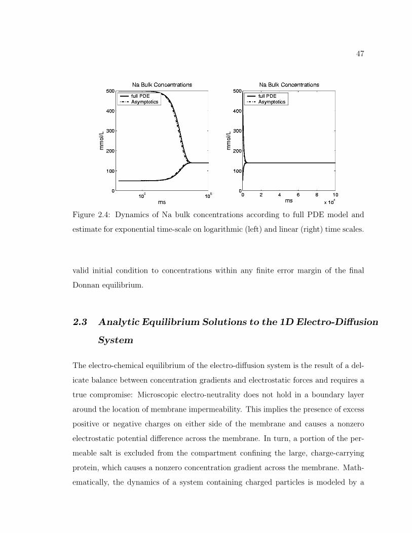
47
Figure 2.4: Dynamics of Na bulk concentrations according to full PDE model and
estimate for exponential time-scale on logarithmic (left) and linear (right) time scales.
valid initial condition to concentrations within any finite error margin of the final
Donnan equilibrium.
2.3 Analytic Equilibrium Solutions to the 1D Electro-Diffusion
System
The electro-chemical equilibrium of the electro-diffusion system is the result of a del-
icate balance between concentration gradients and electrostatic forces and requires a
true compromise: Microscopic electro-neutrality does not hold in a boundary layer
around the location of membrane impermeability. This implies the presence of excess
positive or negative charges on either side of the membrane and causes a nonzero
electrostatic potential difference across the membrane. In turn, a portion of the per-
meable salt is excluded from the compartment confining the large, charge-carrying
protein, which causes a nonzero concentration gradient across the membrane. Math-
ematically, the dynamics of a system containing charged particles is modeled by a
48
system of electro-diffusion and Poisson equations,
∂ci
∂t= ∇ · [Di (∇ci + zici∇ϕ)] (2.31)
∇ · (ε∇ϕ) +∑
i
zici = 0, (2.32)
where a subscript i indicates that a quantity is specific to particle species i, ion species
concentrations are denoted by c, diffusion coefficients by D, species’ valencies by z, the
non-dimensional electrostatic potential by ϕ, and a small, non-dimensional parameter
related to the dielectric coefficient by ε. Using the continuity equation,
∂ci
∂t= −∇ · Ji , (2.33)
in which J denotes flux density, allows us to integrate (2.31) once and replace it by
Nernst−Planck’s equation,
− Ji = Di (∇ci + zici∇ϕ) . (2.34)
At electro-chemical equilibrium Ji = 0 and we can integrate (2.34). The resulting
relationship between concentrations and electrostatic potential is Boltzmann’s law,
∇c · ezϕ + c · z∇ϕ · ezϕ = 0
c (x) ezϕ(x) = c (x0) ezϕ(x0) . (2.35)
When substituted into Poisson’s equation, (2.32), Boltzmann’s law yields the famous
Poisson−Boltzmann equation, a second order, nonlinear partial differential equation
for the electrostatic potential,
∇ · (ε∇ϕ) = −∑
i
zici (x0) exp (−zi (ϕ− ϕ (x0))) , (2.36)
which can be solved explicitly for simple valency constellations in a few select ge-
ometries. We consider a finite-volume, two-compartment system of charges in which
49
the compartments are separated by a thin, homogeneous, semi-permeable, lipid mem-
brane. The membrane has finite width, m, and is impermeable to any confined species
at its mid-point. The dielectric, ε, is piecewise constant with one value valid in free
solution and one in lipid membrane. The diffusion coefficient, D, is assumed piecewise
constant and much larger in free solution than in the membrane. As a result, each of
the compartments equilibrates within itself on a much faster time scale than the one
on which the two compartments interact with each other through the membrane.
In this setting, it is sensible to focus on a region close to mid-membrane and
consider the problem in 1D. A more specific, reasonable definition of “close to mid-
membrane” has to emerge from the problem parameters defining the width of the
membrane as well as the width of the mathematical boundary layer at equilibrium.
In the following, we consider the domain L ≤ x ≤ R for −L = R = m2
> 0 and
mid-membrane located at x = 0. In 1D and for constant diffusion coefficient, D, and
dielectric, ε, the electro-diffusion and Poisson’s equations reduce to
∂ci
∂t= Di
∂
∂x
(∂ci
∂x+ zi
∂ϕ
∂xci
)(2.37)
ε∂2ϕ
∂x2= −
∑i
zici . (2.38)
Using the continuity equation allows to integrate (2.37) once, and we obtain the 1D
version of Nernst−Planck’s equation,
− Ji
Di
=∂ci
∂x+ zi
∂ϕ
∂xci . (2.39)
At equilibrium, Ji = 0 yields Boltzmann’s law, also (2.35),
ci (x) exp (ziϕ (x)) = ci (x0) exp (ziϕ (x0)) , (2.40)
which, in connection with Poisson’s equation, (2.38), leads to the 1D Poisson−Boltzmann
equation,
50
εd2ϕ
dx2= −
∑i
zici (x0) exp (−zi (ϕ− ϕ (x0))) . (2.41)
In 1D, the Poisson−Boltzmann equation is an ordinary differential equation and can
be solved explicitly for various valency combinations of species. Multiplying by dϕdx
yields a first integral to (2.41),
εdϕ
dx· d2ϕ
dx2= −
∑i
ci (x0) zidϕ
dxexp (−zi (ϕ− ϕ (x0))) (2.42)
ε
2
(dϕ
dx
)2
− ε
2
(dϕ
dx(x0)
)2
=∑
i
ci (x0) [exp (−zi (ϕ− ϕ (x0)))− 1] . (2.43)
Choosing x0 = L or x0 = R, the locations of internal or external bulk boundary con-
ditions, it is clear that the electrostatic field there vanishes, dϕdx
(x0) = 0, and that bulk
regions are electro-neutral,∑
i zici (x0) = 0. The actual values of the bulk concentra-
tions are determined from the total mass in the system, as treated in subsection 2.3.1.
Before proceeding, the following notation shall be introduced to combine species of
the same valency:
αx0j =
∑all i
zi = j
ci (x0) . (2.44)
Equation (2.43) may now be written as
ε
2
(dϕ
dx
)2
=
∑i ci (L)
[e−zi(ϕ−ϕ(L)) − 1
]for L < x < 0
∑i ci (R)
[e−zi(ϕ−ϕ(R)) − 1
]for 0 < x < R
(2.45)
ε
2
(dϕ
dx
)2
=
∑j αL
j
[e−j(ϕ−ϕ(L)) − 1
]for L < x < 0
∑j αR
j
[e−j(ϕ−ϕ(R)) − 1
]for 0 < x < R,
(2.46)
51
where the sum is now formed over all valencies, j, in the system rather than individual
species, i. The substitution u = eϕ−ϕ(x0) implies dϕ = duu
and dudx
> 0 ⇔ dϕdx
> 0 and
thus, equation (2.46) becomes
ε
2
(1
u· du
dx
)2
=
∑j αL
j (u−j − 1) for L < x < 0
∑j αR
j (u−j − 1) for 0 < x < R
, and (2.47)
±√
ε
2
du
dx=
√u2∑
j αLj (u−j − 1) for L < x < 0 and ± du
dx> 0
√u2∑
j αRj (u−j − 1) for 0 < x < R and ± du
dx> 0
. (2.48)
In subsections 2.3.2 and 2.3.3, explicit solutions to the separable equation (2.48) shall
be derived for all cases in which valencies are integer and range from −2 to 2, that
is all valencies j ∈ −2;−1; 1; 2. In general, equation (2.48) is solved by a hyper-
elliptic integral that represents an implicit rather than explicit solution. However,
in the cases considered here, the corresponding hyper-elliptic integral can be solved
elegantly and explicitly by factoring the radicand.
2.3.1 Boundary Conditions at Donnan Equilibrium
Before pursuing the details of solving equation (2.48), the correct boundary conditions
shall be derived from the total mass in the system. We need to distinguish between
trapped and permeant species and introduce the following, modified alpha-notation:
αxj =
∑all i
zi = j
ci (x) τxj =
∑trapped i
zi = j
ci (x) αxj = αx
j − τxj . (2.49)
Further, denote the average internal and external concentrations of permeant species
with valency j by αin,outj and that of impermeant species with valency j by τ in,out
j .
52
These values can easily be obtained from any initial condition. Boltzmann’s law
relating the internal and external bulk concentrations of permeant species becomes
αRj ejϕ(R) = αL
j ejϕ(L) (2.50)
for each valency, j, in the system. Mass conservation is correctly formulated as
vinαinj + voutα
outj = (vin − (−L) A) αL
j + A∫ 0
LαL
j e−j(ϕ(x)−ϕ(L))dx + ... (2.51)
... + (vout −RA) αRj + A
∫ R
0αR
j e−j(ϕ(x)−ϕ(R))dx,
where ϕ (x) is the equilibrium profile of the electrostatic potential. Thus, the accurate
solution of the equilibrium problem requires one to solve for the potential profile
and boundary conditions simultaneously. To avoid discretized representations of the
integral in (2.51), it would also be desirable to have explicit expressions for those
integrals available. It is, in fact, possible to obtain analytic expressions for the above
integrals, which are derived and listed in appendix D. For practical purposes and
considering that −L, R vin,out
A, mass conservation may be approximated to high
accuracy by
vinαinj + voutα
outj = vinα
Lj + voutα
Rj . (2.52)
This implies, in particular, that
vinαinj + voutα
outj = vinα
Lj + voutα
Rj
τ inj = τL
j (2.53)
τ outj = τR
j ,
and bulk electro-neutrality gives
∑j
jαLj = −
∑j
jτLj (2.54)
53
∑j
jαRj = −
∑j
jτRj (2.55)
for the internal and external bulk, respectively. Given values αin,outj and τ in,out
j such
that the entire system is electro-neutral and requiring, for example, that the internal
bulk is electro-neutral implies, according to equation (2.52), that the external bulk is
electro-neutral. Thus, only one of the two bulk-electro-neutrality conditions provides
new information. The system to be solved for the boundary conditions, αL,Rj , and the
cross-membrane potential difference, ∆ϕ = ϕ (R)− ϕ (L), is
0 = αRj − αL
j e−j∆ϕ, (2.56)
−∑j
jτ inj =
∑j
jαLj , and (2.57)
vinαinj + voutα
outj = vinα
Lj + voutα
Rj . (2.58)
Alternatively, the system can be expressed as one single, highly nonlinear equation,
(2.59), for the cross-membrane potential, ∆ϕ. Substituting (2.56) into (2.58), solving
the latter for αLj , and substituting the resulting expression for αL
j into (2.57) yields
−∑j
jτ inj =
∑j
jvinα
inj + voutα
outj
vin + voute−j∆ϕ. (2.59)
It will also be required to obtain ∆ϕL = ϕ (0) − ϕ (L) and ∆ϕR = ϕ (0) − ϕ (R)
as parameters for the explicit solution on each side of the domain. Given ∆ϕ, then
∆ϕR = ∆ϕL−∆ϕ and only one equation is needed to determine ∆ϕL. This equation
results from the continuity and smoothness of ϕ at x = 0 and equation (2.46) at x = 0
yields
∑j
αLj
(e−j∆ϕL − 1
)=∑j
αRj
(e−j∆ϕR − 1
)or (2.60)
0 =∑j
αLj
(e−j∆ϕL − 1
)− αR
j
(e−j(∆ϕL−∆ϕ) − 1
), (2.61)
a polynomial equation for e∆ϕL .
54
Example 1: Donnan Exclusion for the Monovalent System
In case of a monovalent system, the only valencies in the system are j = ±1. Substi-
tuting equation (2.56) into (2.57) yields a quadratic for e∆ϕ:
−(τ in1 − τ in
−1
)= αR
1 e∆ϕ − αR−1e
−∆ϕ (2.62)
0 = αR1
(e∆ϕ
)2+(τ in1 − τ in
−1
)e∆ϕ − αR
−1 (2.63)
(e∆ϕ
)1,2
=−(τ in1 − τ in
−1
)±√
(τ in1 − τ in
−1)2+ 4αR
1 αR−1
2αR1
. (2.64)
Since e∆ϕ > 0, the root corresponding to the plus sign is the correct one and
e∆ϕ =−(τ in1 − τ in
−1
)+√
(τ in1 − τ in
−1)2+ 4αR
1 αR−1
2αR1
. (2.65)
For a relatively small amount of trapped net charge, that is∣∣∣τ in
1 − τ in−1
∣∣∣ √αR
1 αR−1, the
quadratic term may be neglected, and the internal, permeant species concentrations
are approximated by
αL1 = αR
1 e∆ϕ = −τ in1 − τ in
−1
2+
√√√√(τ in1 − τ in
−1
2
)2
+ αR1 αR
−1 (2.66)
≈ −τ in1 − τ in
−1
2+√
αR1 αR
−1. (2.67)
When trapped net charges are present in the internal region, the concentrations of
the internal, permeant species are depleted by approximately half the concentration
of those trapped net charges. This is known as the famous Donnan exclusion.
Example 2: Boundary Conditions for the Monovalent System
In case of a monovalent system, the only valencies in the system are j = ±1, thus
equation (2.59) is a quadratic for W = e∆ϕ. For convenience, the abbreviations
Tin,out = τ in,out1 − τ in,out
−1 and Aj = vinαinj + voutα
outj shall be used. Then,
55
− Tin =A1
vin + voutW−1− A−1
vin + voutWand (2.68)
− Tin
(vin + voutW
−1)
(vin + voutW ) = A1 (vin + voutW )− A−1
(vin + voutW
−1).
(2.69)
Collecting terms of the same power of W , the resulting standard quadratic is
0 = AW 2 + BW + C, where (2.70)
A = A1vout + Tinvinvout ,
B =(A1 − A−1
)vin + Tin
(v2
in + v2out
), (2.71)
C = −A−1vout + Tinvinvout , and
W1,2 =−B ±
√B2 − 4AC
2A. (2.72)
It is reasonable to assume that less mass is trapped in the internal compartment
than there is mass of valencies 1 or −1 in the entire system, that is A1 > Tinvin and
A−1 > Tinvin. Therefore, A > 0, C < 0, and the sign of B is undetermined. W has
to be positive, so the root corresponding to the plus sign is the correct one to choose.
After some algebra to simplify, we obtain
W =1
2vout
(A1 + Tinvin
) − [(A1 − A−1
)vin + Tin
(v2
in + v2out
)](2.73)
+
√[(A1 + A−1
)vin + Tin (v2
in − v2out)
]2− 4A−1
(A1 + Tinvin
)(v2
in − v2out)
.
In case vin = vout,
W =−(A1 − A−1
)vin − Tin (v2
in + v2out) +
(A1 + A−1
)vin
2vout
(A1 + Tinvin
)
56
=2vinA−1 − 2Tinv
2in
2vout
(A1 + Tinvin
) (2.74)
=A−1 − Tinvin
A1 + Tinvin
=A1 + Toutvout
A1 + Tinvin
,
where we have used that A1 − A−1 = − (Tinvin + Toutvout). The relative sizes of the
amounts of internally and externally trapped net charges to the amount of permeant
mass in the system are clearly and intricately related to the cross-membrane potential.
When no trapped species are present, it is easy to see that the trivial equilibrium with
∆ϕ = 0 results.
2.3.2 Equilibrium Solution With Valency j=-2 in the System
Since equation (2.48) is essentially the same in both regions of the domain, the su-
perscripts L, R are dropped from the alpha-notation and it is understood that results
are restricted to their respective sides of the domain. When all considered valencies
are present in the system,
±√
ε
2
du
dx=√
u2 [α−2 (u2 − 1) + α−1 (u− 1) + α1 (u−1 − 1) + α2 (u−2 − 1)] , (2.75)
±√
ε
2
du
dx=√
α−2u4 + α−1u3 − (α−2 + α−1 + α1 + α2) u2 + α1u + α2 , (2.76)
for ±dudx
> 0. It is easily verified that u = 1 is a root of the radicand in (2.76).
Performing a polynomial division of the radicand by the factor u− 1 yields
α−2u4 + α−1u
3 − (α−2 + α−1 + α1 + α2) u2 + α1u + α2 =
(u− 1) (α−2u3 + (α−2 + α−1) u2 − (α1 + α2) u− α2) .
(2.77)
57
Bulk electro-neutrality implies 2α−2 + α−1 = 2α2 + α1 and thus, the second factor in
(2.77) also has u = 1 as a root. Performing a second polynomial division and taking
the electro-neutrality condition into account, the original radicand may be written as
α−2u4 + α−1u
3 − (α−2 + α−1 + α1 + α2) u2 + α1u + α2 =
(u− 1)2 (α−2u2 + (2α−2 + α−1) u + α2) .
(2.78)
The last factor in (2.78) is quadratic in u and has roots at u = u1,2. The original
radicand may thus be expressed as
α−2u4 + α−1u
3 − (α−2 + α−1 + α1 + α2) u2 + α1u + α2 =
α−2 (u− 1)2 (u− u1) (u− u2) , where(2.79)
u1,2 =1
2α−2
[− (2α−2 + α−1)±
√(2α−2 + α−1)
2 − 4α−2α2
]≤ 0. (2.80)
Equation (2.76) now reduces to
±√
ε
2
du
dx=√
α−2 |u− 1|√
(u− u1) (u− u2) , (2.81)
±√
2α−2
εdx =
du
|u− 1|√
(u− u1) (u− u2), (2.82)
for ±dudx
> 0. To simplify the absolute value and case distinction, recall that dudx
>
0 ⇔ dϕdx
> 0 and that the sign of dϕdx
is determined by Gauss’ law through the sign of
the net charge in the considered region. Applying Gauss’ law to the internal region
and recalling that dϕdx
(L) = 0,
ε
(∂ϕ
∂x(0)− ∂ϕ
∂x(L)
)∝ − (internal net charge) , (2.83)
ε∂ϕ
∂x(0) ∝ − (internal net charge) . (2.84)
Analogously, for the external region and dϕdx
(R) = 0,
ε
(∂ϕ
∂x(R)− ∂ϕ
∂x(0)
)∝ − (external net charge) , (2.85)
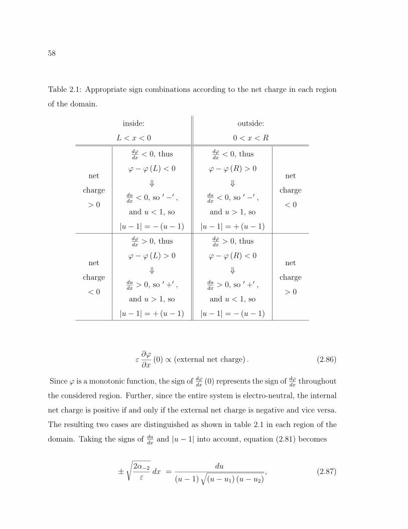
58
Table 2.1: Appropriate sign combinations according to the net charge in each region
of the domain.
inside:
L < x < 0
outside:
0 < x < R
net
charge
> 0
dϕdx
< 0, thus
ϕ− ϕ (L) < 0
⇓dudx
< 0, so ′ −′ ,
and u < 1, so
|u− 1| = − (u− 1)
dϕdx
< 0, thus
ϕ− ϕ (R) > 0
⇓dudx
< 0, so ′ −′ ,
and u > 1, so
|u− 1| = + (u− 1)
net
charge
< 0
net
charge
< 0
dϕdx
> 0, thus
ϕ− ϕ (L) > 0
⇓dudx
> 0, so ′ +′ ,
and u > 1, so
|u− 1| = + (u− 1)
dϕdx
> 0, thus
ϕ− ϕ (R) < 0
⇓dudx
> 0, so ′ +′ ,
and u < 1, so
|u− 1| = − (u− 1)
net
charge
> 0
ε∂ϕ
∂x(0) ∝ (external net charge) . (2.86)
Since ϕ is a monotonic function, the sign of dϕdx
(0) represents the sign of dϕdx
throughout
the considered region. Further, since the entire system is electro-neutral, the internal
net charge is positive if and only if the external net charge is negative and vice versa.
The resulting two cases are distinguished as shown in table 2.1 in each region of the
domain. Taking the signs of dudx
and |u− 1| into account, equation (2.81) becomes
±√
2α−2
εdx =
du
(u− 1)√
(u− u1) (u− u2), (2.87)
59
where now the positive sign is valid in the internal region and the negative sign in the
external region of the domain. Integrating both sides of (2.87) from x = 0 outward,
denoting u0 = u (0), and u = u (x),
±∫ x
0
√2α−2
εdx =
∫ u
u0
du
(u− 1)√
(u− u1) (u− u2), (2.88)
±√
2α−2
εx =
1√cln
(u−1)
(u0−1)·
(2
√c(u0−u1)(u0−u2)+2c+b(u0−1)
)(
2√
c(u−u1)(u−u2)+2c+b(u−1)
) for u1 6= u2
1√cln[
(u−1)
(u0−1)· (2c+b(u0−1))
(2c+b(u−1))
]for u1 = u2
,
(2.89)
where b = (1− u1) + (1− u2), c = (1− u1) (1− u2), and u1 = u2 ⇔ 4α−2α2 =
(2α−2 + α−1)2. Solving each case for u explicitly yields a quadratic equation for
u1 6= u2 and a linear equation for u1 = u2. Note that ±√
2α−2
εx < 0 for all L < x < R
and make use of the following notation:
σ =
+√
2cα−2
εfor L < x < 0
−√
2cα−2
εfor 0 < x < R
(2.90)
L (u) =
u−1
2√
c(u−u1)(u−u2)+2c+b(u−1)for u1 6= u2
u−12c+b(u−1)
for u1 = u2
(2.91)
Λ (x) = L (u0) exp (σx) . (2.92)
Then u is a solution of
Λ (x) = L (u) . (2.93)
60
Explicit Solution in Case u1 6= u2:
In case u1 6= u2, equation (2.93) is a quadratic equation for u,
Λ =u− 1
2√
c (u− u1) (u− u2) + 2c + b (u− 1)(2.94)
(2√
c (u− u1) (u− u2) + 2c + b (u− 1))
Λ = u− 1 (2.95)
2Λ√
c (u− u1) (u− u2) = (u− 1)− (2c + b (u− 1)) Λ (2.96)
2Λ√
c (u− u1) (u− u2) = (u− 1) (1− bΛ)− 2cΛ (2.97)
2√
c (u− u1) (u− u2) = (u− 1)(Λ−1 − b
)− 2c (2.98)
4c (u− u1) (u− u2) =
(u− 1)2 (Λ−1 − b)2 − 4c (u− 1) (Λ−1 − b) + 4c2
(2.99)
4c (u2 − (u1 + u2) u + u1u2) =
(u2 − 2u + 1) (Λ−1 − b)2 − 4c (u− 1) (Λ−1 − b) + 4c2.
(2.100)
Collecting terms proportional to the powers of u yields a standard quadratic,
0 = Au2 −Bu + C, where (2.101)
A =(Λ−1 − b
)2− 4c
B = 2(Λ−1 − b
)2+ 4c
(Λ−1 − b
)− 4c (u1 + u2) (2.102)
C =((
Λ−1 − b)
+ 2c)2− 4cu1u2 , and
u =B ±
√B2 − 4AC
2A. (2.103)
61
Using that u1 + u2 = 2− b and u1u2 = 1− b + c, we can simplify B and C:
B = 2(Λ−1 − b
)2+ 4c
(Λ−1 − b
)− 4c (2− b)
= 2((
Λ−1 − b)2− 4c
)+ 4c
((Λ−1 − b
)+ b
)(2.104)
= 2A + 4cΛ−1 and
C =[(
Λ−1 − b)
+ 2c]2− 4c (1− b + c)
=(Λ−1 − b
)2+ 4c
(Λ−1 − b
)+ 4c2 − 4c (1− b + c) (2.105)
=(Λ−1 − b
)2− 4c + 4cΛ−1
= A + 4cΛ−1.
The relations (2.104) and (2.105) are used to simplify the term B2 − 4AC:
B2 − 4AC =(2A + 4cΛ−1
)2− 4AC
= 4A2 + 16cΛ−1A + 16c2Λ−2 − 4AC (2.106)
= 16c2Λ−2 + 4A(A + 4cΛ−1 − C
)= 16c2Λ−2.
With these simplifications, the two possible solutions for u are
u =2A + 4cΛ−1 ±
√16c2Λ−2
2A. (2.107)
The solution related to the negative sign is the trivial solution, u (x) = 1. Therefore,
the other root is selected and the explicit equilibrium solution can be written in the
following, equivalent forms:
u = 1 +4cΛ−1
A
62
= 1 +4cΛ−1
(Λ−1 − b)2 − 4c(2.108)
= 1 +4cΛ
(1− bΛ)2 − 4cΛ2.
Explicit Solution in Case u1 = u2:
In case u1 = u2, equation (2.93) is a linear equation for u, namely
Λ =u− 1
2c + b (u− 1)(2.109)
(2c + b (u− 1)) Λ = u− 1 (2.110)
2cΛ = (u− 1) (1− bΛ) . (2.111)
The explicit solution may thus be written in the following, equivalent forms:
u = 1 +2c
Λ−1 − b(2.112)
= 1 +2cΛ
1− bΛ.
2.3.3 Equilibrium Solution Without Valency j=-2 in the System
Since equation (2.48) is essentially the same in both regions of the domain, the su-
perscripts L, R are dropped from the alpha-notation and it is understood that results
are restricted to their respective sides of the domain. When any of the considered
valencies except j = −2 are present in the system, then
±√
ε
2
du
dx=√
u2 [α−1 (u− 1) + α1 (u−1 − 1) + α2 (u−2 − 1)] , (2.113)
±√
ε
2
du
dx=√
α−1u3 − (α−2 + α−1 + α1 + α2) u2 + α1u + α2 , (2.114)
63
for ±dudx
> 0. It is easily verified that u = 1 is a root of the radicand in (2.114).
Performing a polynomial division of the radicand by the factor u− 1 yields
α−1u3 − (α−2 + α−1 + α1 + α2) u2 + α1u + α2 =
(u− 1) (α−1u2 − (α1 + α2) u− α2) .
(2.115)
The last factor in (2.115) is quadratic in u, has one root at u = 1 because 2α2 + α1 =
α−1, and the other root at u = u2. The original radicand may thus be expressed as
α−1u3 − (α−2 + α−1 + α1 + α2) u2 + α1u + α2 =
α−1 (u− 1)2 (u− u2) , where(2.116)
u2 =−α2
α1 + 2α2
≤ 0. (2.117)
Equation (2.114) now reduces to
±√
ε
2
du
dx=√
α−1 |u− 1|√
u− u2 , (2.118)
±√
2α−1
εdx =
du
|u− 1|√
u− u2
, (2.119)
for ±dudx
> 0. The table in subsection 2.3.2 is valid in this case, too, and the absolute
value and case distinction are reduced accordingly. Equation (2.119) becomes
±√
2α−1
εdx =
du
(u− 1)√
u− u2
, (2.120)
where the positive sign is valid in the internal region and the negative sign in the
external region of the domain. Integrating both sides of (2.120) from x = 0 outward,
denoting u0 = u (0), and u = u (x),
±∫ x
0
√2α−1
εdx =
∫ u
u0
du
(u− 1)√
u− u2
, (2.121)
64
±√
2α−1
εx =
1√1− u2
ln
(√
u− u2 −√
1− u2
)(√
u− u2 +√
1− u2
) ·(√
u0 − u2 +√
1− u2
)(√
u0 − u2 −√
1− u2
) . (2.122)
Solving for u explicitly yields a quadratic equation. Note that ±√
2α−1
εx < 0 for all
L < x < R and make use of the following notation:
σ =
+√
2(1−u2)α−1
εfor L < x < 0
−√
2(1−u2)α−1
εfor 0 < x < R
(2.123)
L (u) =
√u− u2 −
√1− u2√
u− u2 +√
1− u2
(2.124)
Λ (x) = L (u0) exp (σx) . (2.125)
Then u is a solution of
Λ (x) = L (u) . (2.126)
To obtain an explicit solution for u in the considered case, the quadratic equation,
(2.126), is solved:
Λ =
√u− u2 −
√1− u2√
u− u2 +√
1− u2
(2.127)
(√u− u2 +
√1− u2
)Λ =
√u− u2 −
√1− u2 (2.128)
√u− u2 (Λ− 1) = −
√1− u2 (Λ + 1) (2.129)
√u− u2 =
√1− u2
1 + Λ
1− Λ(2.130)
65
u = u2 + (1− u2)(
1 + Λ
1− Λ
)2
. (2.131)
In the special case of only monovalent species (valencies ±1) in the system, u2 = 0
and solution (2.131) reduces to
u =(
1 + Λ
1− Λ
)2
. (2.132)
66
Chapter 3
DYNAMIC APPROACH TO DONNAN EQUILIBRIUM
It shall be verified numerically in this chapter, for the example of the dynamic
approach to Donnan equilibrium, that the transient electro-diffusion system is ap-
proximated well by quasi steady-state dynamics. Since the electro-diffusion system
is much more efficiently simulated in case of mid-membrane impermeability (see also
section 2.1), this chapter shall be restricted to this setting. The numeric simulation
of the transient, nonlinear electro-diffusion equations is addressed in section 3.1. This
is followed, in section 3.2, by the numeric solution of the steady-state problem as-
sociated with the quasi steady-state approximation (QSSA). Section 3.3 treats the
implementation of the quasi steady-state approximation and compares its dynamics
to the dynamics of the fully transient system. Results are summarized in section 3.4.
3.1 Numeric Solution of Transient Electro-Diffusion System
As discussed in section 2.1, the internal and external bulk concentrations, c (−L) and
c (R), are assumed constant and we focus on the dynamics in the membrane region
in 1D. The width of the membrane is m = 2√
ε, that is the mathematical boundary
layer is filled with membrane medium. Recall the electro-diffusion system to be solved
in 1D,
∂ci
∂t= Di
∂
∂x
(∂ci
∂x+ zi
∂ϕ
∂xci
)(3.1)
ε∂2ϕ
∂x2+∑
i
zici = 0, (3.2)
67
for x ∈[−m
2; m
2
], where D and ε are the diffusion and dielectric coefficients associ-
ated with the membrane medium. The bulk concentrations, c (−L) and c (R), are
the boundary conditions for (3.1) and are updated via ordinary differential equations
involving the compartment volumes and flux densities across the membrane bound-
aries at ±m2. The latter ensures zero-flux out of the system boundaries and thus mass
conservation and charge conservation in the entire system. In addition to zero-flux
conditions at the system boundaries, impermeant ion species obey zero-flux conditions
at mid-membrane, x = 0. Boundary conditions (2.13) are used on the electrostatic
potential,
ϕ (−L) = 0 and∂ϕ
∂x(R) = 0. (3.3)
It is because of the additional zero-flux boundary conditions for impermeant species
within the domain that we are not able to use any of the, otherwise available, standard
packages for the numeric simulation of partial differential equations. None of the
standard packages investigated allows the specification of such additional boundary
conditions. Therefore, in the following, the discretization of the mathematical domain
and various finite-difference methods for solving (3.1) and (3.2) numerically shall be
introduced and discussed.
3.1.1 Discretization of the Domain
The mathematical domain is subdivided uniformly and variables are assigned and
indexed as shown in figure 3.1. It is understood that the natural length scales of
each compartment are R − m2
= vout
Aand L − m
2= vin
A, where vin,out denote the
volumes of compartments and A is the surface area of the semi-permeable membrane.
The domain is, in particular, divided into equal sub-intervals by uniformly spaced
interfaces. At the center of each sub-interval there lies a node. With an even number,
N , of nodes in the discretization lying within the membrane region, the distance
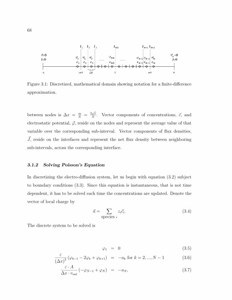
68
Figure 3.1: Discretized, mathematical domain showing notation for a finite-difference
approximation.
between nodes is ∆x = mN
= 2√
εN
. Vector components of concentrations, ~c, and
electrostatic potential, ~ϕ, reside on the nodes and represent the average value of that
variable over the corresponding sub-interval. Vector components of flux densities,
~J , reside on the interfaces and represent the net flux density between neighboring
sub-intervals, across the corresponding interface.
3.1.2 Solving Poisson’s Equation
In discretizing the electro-diffusion system, let us begin with equation (3.2) subject
to boundary conditions (3.3). Since this equation is instantaneous, that is not time
dependent, it has to be solved each time the concentrations are updated. Denote the
vector of local charge by
~a =∑
species i
zi~ci. (3.4)
The discrete system to be solved is
ϕ1 = 0 (3.5)
ε
(∆x)2 (ϕk−1 − 2ϕk + ϕk+1) = −ak for k = 2, ..., N − 1 (3.6)
ε · A∆x · vout
(−ϕN−1 + ϕN) = −aN , (3.7)
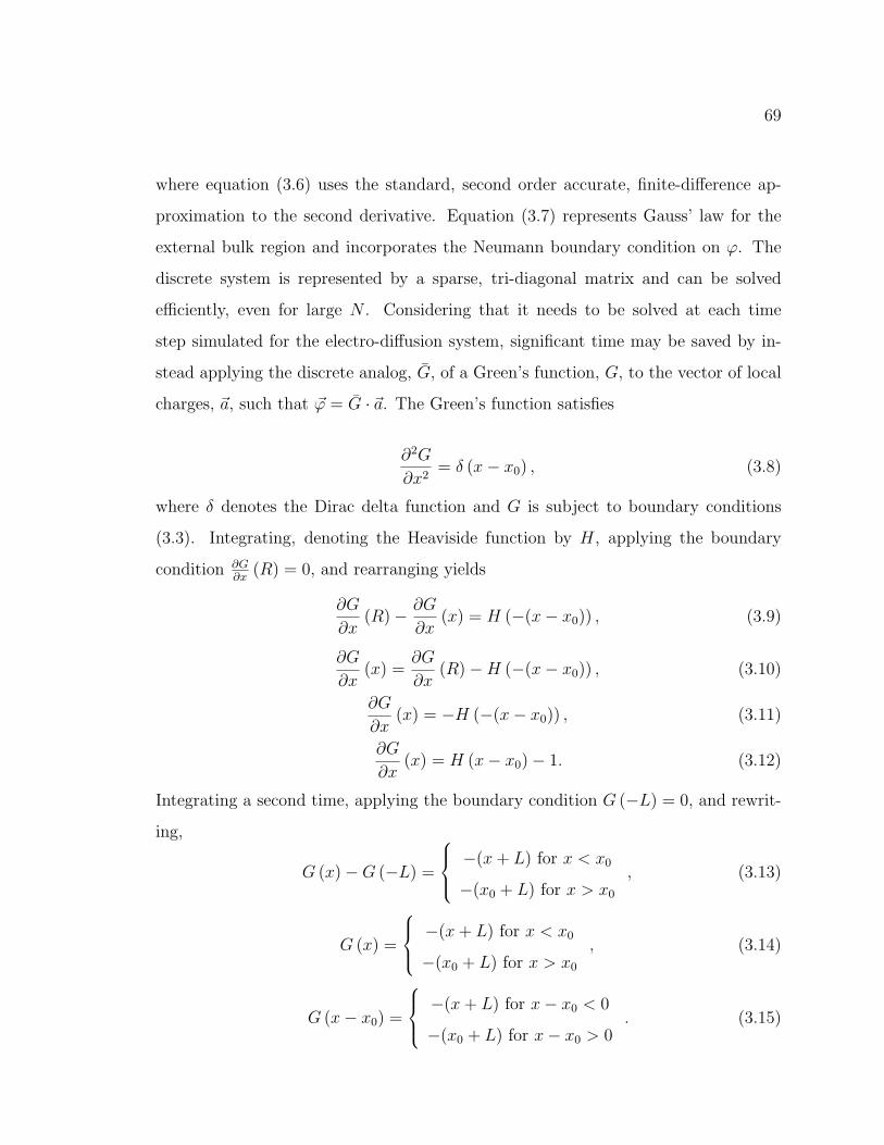
69
where equation (3.6) uses the standard, second order accurate, finite-difference ap-
proximation to the second derivative. Equation (3.7) represents Gauss’ law for the
external bulk region and incorporates the Neumann boundary condition on ϕ. The
discrete system is represented by a sparse, tri-diagonal matrix and can be solved
efficiently, even for large N . Considering that it needs to be solved at each time
step simulated for the electro-diffusion system, significant time may be saved by in-
stead applying the discrete analog, G, of a Green’s function, G, to the vector of local
charges, ~a, such that ~ϕ = G · ~a. The Green’s function satisfies
∂2G
∂x2= δ (x− x0) , (3.8)
where δ denotes the Dirac delta function and G is subject to boundary conditions
(3.3). Integrating, denoting the Heaviside function by H, applying the boundary
condition ∂G∂x
(R) = 0, and rearranging yields
∂G
∂x(R)− ∂G
∂x(x) = H (−(x− x0)) , (3.9)
∂G
∂x(x) =
∂G
∂x(R)−H (−(x− x0)) , (3.10)
∂G
∂x(x) = −H (−(x− x0)) , (3.11)
∂G
∂x(x) = H (x− x0)− 1. (3.12)
Integrating a second time, applying the boundary condition G (−L) = 0, and rewrit-
ing,
G (x)−G (−L) =
−(x + L) for x < x0
−(x0 + L) for x > x0
, (3.13)
G (x) =
−(x + L) for x < x0
−(x0 + L) for x > x0
, (3.14)
G (x− x0) =
−(x + L) for x− x0 < 0
−(x0 + L) for x− x0 > 0. (3.15)
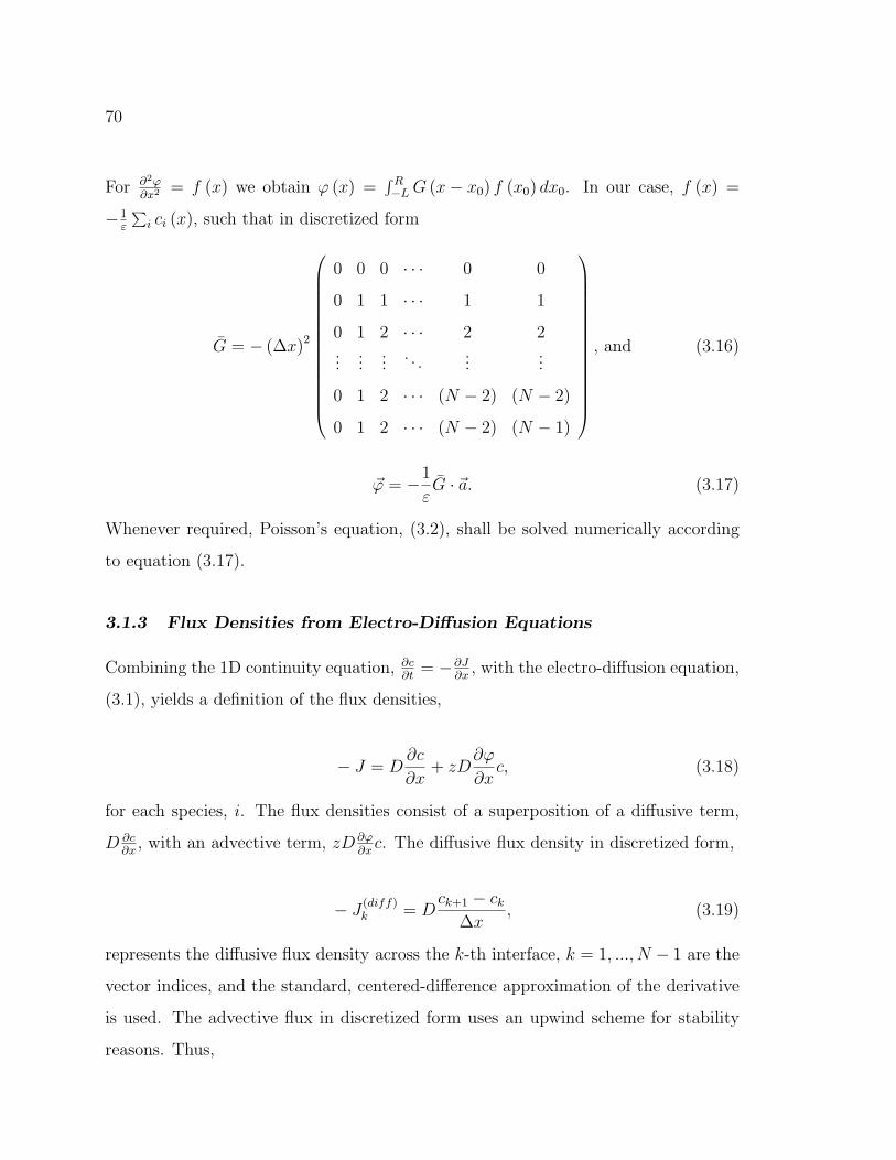
70
For ∂2ϕ∂x2 = f (x) we obtain ϕ (x) =
∫ R−L G (x− x0) f (x0) dx0. In our case, f (x) =
−1ε
∑i ci (x), such that in discretized form
G = − (∆x)2
0 0 0 · · · 0 0
0 1 1 · · · 1 1
0 1 2 · · · 2 2...
......
. . ....
...
0 1 2 · · · (N − 2) (N − 2)
0 1 2 · · · (N − 2) (N − 1)
, and (3.16)
~ϕ = −1
εG · ~a. (3.17)
Whenever required, Poisson’s equation, (3.2), shall be solved numerically according
to equation (3.17).
3.1.3 Flux Densities from Electro-Diffusion Equations
Combining the 1D continuity equation, ∂c∂t
= −∂J∂x
, with the electro-diffusion equation,
(3.1), yields a definition of the flux densities,
− J = D∂c
∂x+ zD
∂ϕ
∂xc, (3.18)
for each species, i. The flux densities consist of a superposition of a diffusive term,
D ∂c∂x
, with an advective term, zD ∂ϕ∂x
c. The diffusive flux density in discretized form,
− J(diff)k = D
ck+1 − ck
∆x, (3.19)
represents the diffusive flux density across the k-th interface, k = 1, ..., N − 1 are the
vector indices, and the standard, centered-difference approximation of the derivative
is used. The advective flux in discretized form uses an upwind scheme for stability
reasons. Thus,
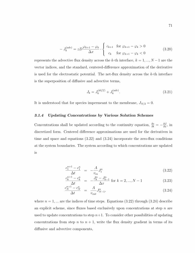
71
− J(adv)k = zD
ϕk+1 − ϕk
∆x·
ck+1 for ϕk+1 − ϕk > 0
ck for ϕk+1 − ϕk < 0(3.20)
represents the advective flux density across the k-th interface, k = 1, ..., N −1 are the
vector indices, and the standard, centered-difference approximation of the derivative
is used for the electrostatic potential. The net-flux density across the k-th interface
is the superposition of diffusive and advective terms,
Jk = J(diff)k + J
(adv)k . (3.21)
It is understood that for species impermeant to the membrane, JN/2 = 0.
3.1.4 Updating Concentrations by Various Solution Schemes
Concentrations shall be updated according to the continuity equation, ∂c∂t
= −∂J∂x
, in
discretized form. Centered difference approximations are used for the derivatives in
time and space and equations (3.22) and (3.24) incorporate the zero-flux conditions
at the system boundaries. The system according to which concentrations are updated
is
cn+11 − cn
1
∆t= − A
vin
Jn1 (3.22)
cn+1k − cn
k
∆t= −
Jnk − Jn
k−1
∆xfor k = 2, ..., N − 1 (3.23)
cn+1N − cn
N
∆t=
A
vout
JnN−1, (3.24)
where n = 1, ... are the indices of time steps. Equations (3.22) through (3.24) describe
an explicit scheme, since fluxes based exclusively upon concentrations at step n are
used to update concentrations to step n+1. To consider other possibilities of updating
concentrations from step n to n + 1, write the flux density gradient in terms of its
diffusive and advective components,
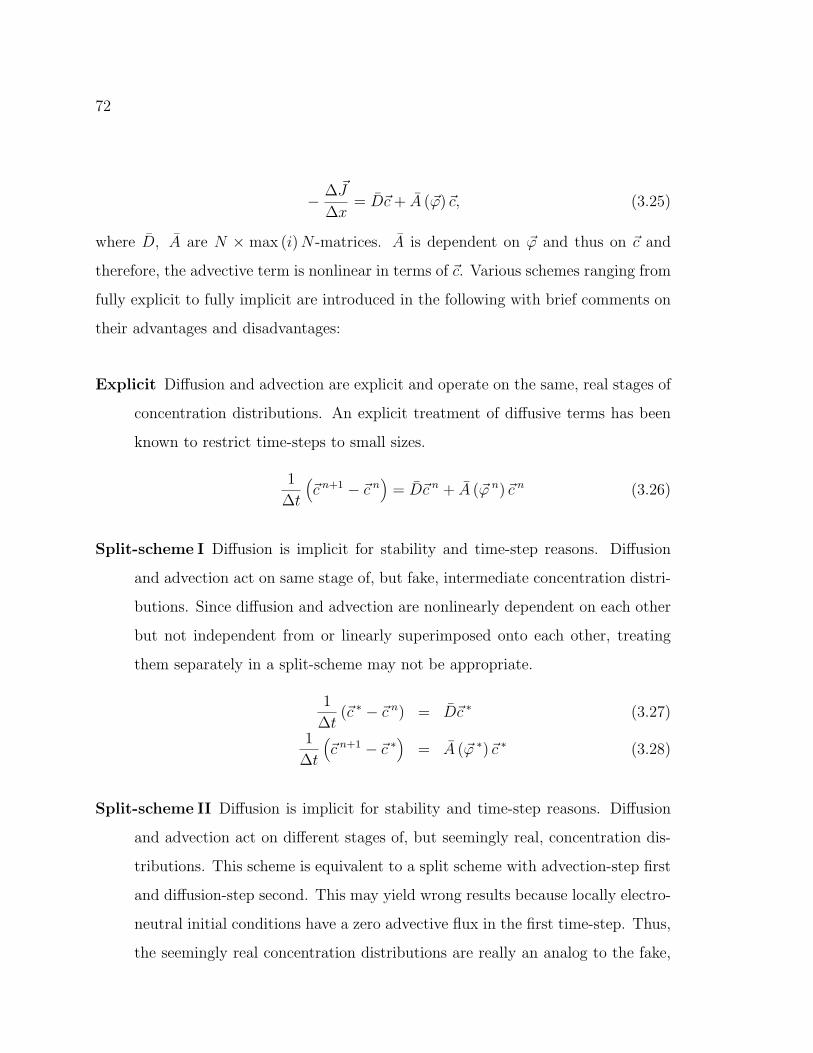
72
− ∆ ~J
∆x= D~c + A (~ϕ)~c, (3.25)
where D, A are N × max (i) N -matrices. A is dependent on ~ϕ and thus on ~c and
therefore, the advective term is nonlinear in terms of ~c. Various schemes ranging from
fully explicit to fully implicit are introduced in the following with brief comments on
their advantages and disadvantages:
Explicit Diffusion and advection are explicit and operate on the same, real stages of
concentration distributions. An explicit treatment of diffusive terms has been
known to restrict time-steps to small sizes.
1
∆t
(~c n+1 − ~c n
)= D~c n + A (~ϕ n)~c n (3.26)
Split-scheme I Diffusion is implicit for stability and time-step reasons. Diffusion
and advection act on same stage of, but fake, intermediate concentration distri-
butions. Since diffusion and advection are nonlinearly dependent on each other
but not independent from or linearly superimposed onto each other, treating
them separately in a split-scheme may not be appropriate.
1
∆t(~c ∗ − ~c n) = D~c ∗ (3.27)
1
∆t
(~c n+1 − ~c ∗
)= A (~ϕ ∗)~c ∗ (3.28)
Split-scheme II Diffusion is implicit for stability and time-step reasons. Diffusion
and advection act on different stages of, but seemingly real, concentration dis-
tributions. This scheme is equivalent to a split scheme with advection-step first
and diffusion-step second. This may yield wrong results because locally electro-
neutral initial conditions have a zero advective flux in the first time-step. Thus,
the seemingly real concentration distributions are really an analog to the fake,
73
half-step concentrations of split-scheme I. In addition, treating diffusion and
advection independently may not be appropriate, as outlined above.
1
∆t
(~c n+1 − ~c n
)= D~c n+1 + A (~ϕ n)~c n (3.29)
Semi-implicit This scheme is closest to an implicit scheme while each time step
is still solvable as a linear system. Diffusion and advection are implicit, while
the electrostatic potential is from the previous time-step. Thus, diffusion and
advection are not treated independently from each other. Conditions for time-
step restriction are not straight-forward but test runs suggest a much higher
efficiency than the explicit scheme.
1
∆t
(~c n+1 − ~c n
)= D~c n+1 + A (~ϕ n)~c n+1 (3.30)
Implicit This scheme is represented by a nonlinear system. While time-step restric-
tion is more simple compared to the semi-implicit scheme, the implicit scheme
requires a Newton-type iteration to be solved at each time-step.
1
∆t
(~c n+1 − ~c n
)= D~c n+1 + A
(~ϕ n+1
)~c n+1 (3.31)
We shall not use a split-scheme for our numerical simulations. This is due to concerns
of an inadequate separation of diffusion and advection when both processes are clearly
interdependent. While the semi-implicit scheme shows promise both in accuracy
and efficiency, the derivation of quality ensuring time-step restrictions is not straight
forward. The implicit scheme, in contrast, has relatively simple time-step restrictions
but its efficiency suffers by requiring a nonlinear system to be solved at each time-
step. Thus, the explicit scheme, solvable as a linear system with restrictive yet clear
guidelines for time-step selection, shall be used for our purposes.

74
3.1.5 Time-Step Restrictions and Numeric Diffusion
It is demonstrated next, that the explicit scheme is dominated by diffusion with
respect to its time-step restriction. Further, an estimate will be obtained for the size
of numeric diffusion introduced by the upwind scheme used to obtain the advective
flux. While providing much greater stability to the numeric solution process, the
upwind scheme is known to introduce a certain amount of artificial, numeric diffusion.
To obtain accurate results, the size of numeric diffusion needs to be much smaller than
the size of actual diffusion in the problem. Thus,
1
2
∣∣∣a∆x− a2∆t∣∣∣ D (3.32)
at every point in the discretized domain, where a =∣∣∣zD∆ϕ
∆x
∣∣∣ = D |z∆ϕ|∆x
, the local
advection velocity. The following constraints apply:
• diffusion: ∆t = α∆x2
2D(0 < α < 1),
• advection: ∆t = ν ∆xa
(ν < 1, and a = D |z∆ϕ|∆x
),
• numeric diffusion: 12|a∆x− a2∆t| D.
Suppose an explicit scheme is used and diffusion dictates the time step, then
α∆x2
2D< ν
∆x
a⇒ |z∆ϕ| < 2
ν
α, where ν, α < 1. (3.33)
For ν, α = 0.9, this implies |z∆ϕ| < 2. Consider a cross-membrane potential dif-
ference of −70 mV, that is a difference between the boundary values of ϕ of about
70/27 due to the non-dimensionalizing scaling, R0TF≈ 27 mV. The transition of the
electrostatic potential from its internal to its external value occurs effectively over
about one eighth of the domain, so that, in a monovalent system, |z∆ϕ|∆x
ranges from
0 to about (70/27)(N∆x/8)
. Considering a grid with N = 100 nodes implies 0 < |z∆ϕ| < 0.2.
75
Clearly, |z∆ϕ| < 2 and lies within the region in which diffusion dictates the time-step
restriction. It has hereby been demonstrated and is expected that diffusion dominates
the time-step restriction in actual simulations of the electro-diffusion system.
Regarding the numeric diffusion, it is desired that
a
2D|∆x− a∆t| 1 ⇒ |z∆ϕ|
2∆x
∣∣∣∣∣∆x−D|z∆ϕ|∆x
α∆x2
2D
∣∣∣∣∣ 1 (3.34)
⇒ 1
2|z∆ϕ|
∣∣∣∣1− α
2|z∆ϕ|
∣∣∣∣ 1. (3.35)
The expression in (3.35) represents the relative size of numeric to actual diffusion and
has roots at |z∆ϕ| = 0 and |z∆ϕ| = 2α. According to equation (3.33), |z∆ϕ| lies
between the two roots. The local maximum of, or worst case, numeric diffusion lies
at |z∆ϕ| = 1α
and equals
1
2α
∣∣∣∣1− 1
2
∣∣∣∣ = 1
4α, where
1
4α 1. (3.36)
To minimize the worst case numeric diffusion, one should pick α < 1 as large as
possible. One can, however, easily see that the worst case numeric diffusion equals
at least 25% of the true diffusion. For example, for α = 0.9, the worst case numeric
diffusion equals about 28% of the true diffusion.
This worst case scenario only provides an upper bound on numeric diffusion and
may not reflect the operating conditions for actual simulations. To obtain a more
meaningful and realistic estimate for the numeric diffusion in actual simulations, re-
consider a cross-membrane potential difference of −70 mV over a domain discretized
by N = 100 nodes. With α = 0.9, |z∆ϕ| < 0.2 does not reach 1α≈ 1.11, its value for
worst case numerical diffusion. Thus, the maximum numerical diffusion occurs at the
location in the domain where |z∆ϕ| = 0.2 and equals 12|z∆ϕ|
∣∣∣1− α2|z∆ϕ|
∣∣∣ ≈ 0.06,
approximately 6% of the true diffusion.
76
3.2 Numeric Solution of the Steady-State Problem Using
an “Almost-Newton” Method
In this section, the steady-state of a 1D electro-diffusion system, (3.37) and (3.38),
shall be solved numerically.
∂ci
∂t=
∂
∂x
(Di
∂ci
∂x+ ziDi
∂ϕ
∂xci
)(3.37)
∂
∂x
(ε∂ϕ
∂x
)= −
∑i
zici , (3.38)
where subscripts i indicate that a quantity is specific to ionic species i, c denotes par-
ticle concentrations, D diffusion coefficients, z valencies, ϕ the non-dimensionalized
electrostatic potential, and ε a non-dimensional quantity related to the dielectric of
the membrane. Our domain of interest is L ≤ x ≤ R, where R, − L > 0 and the
membrane midpoint lies at x = 0. Boundary conditions on particle concentrations
are
ci (L) = cLi and ci (R) = cR
i for all species i. (3.39)
Natural boundary conditions on the electrostatic potential are, as discussed in sub-
section 2.1.2, given by Gauss’ law,
ϕx (L) = 0 = ϕx (R) . (3.40)
In general, (3.40) does not define a mathematically well-posed problem but since the
electrostatic potential, ϕ, is only determined up to a constant, we may prescribe any
value, Φ, at one location, x0, such that ϕ (x0) = Φ. For convenience, Φ = 0 and
we obtain two sets of boundary conditions, each of which defines a mathematically
different but well-posed problem:
77
ϕ (L) = 0 and ϕx (R) = 0, (3.41)
ϕx (L) = 0 and ϕ (R) = 0. (3.42)
The respective other Neumann condition is automatically satisfied. The issues with
boundary conditions have been explored in subsection 2.1.2 and will be investigated
numerically in section 3.2. Next, flux densities, Ji, and concentration distributions,
ci, shall be derived as functions of the electrostatic potential, ϕ. From the continuity
equation, at steady-state∂ci
∂t= −∂Ji
∂x= 0 . (3.43)
Therefore, the flux density Ji (x) = Ji = const. and the electro-diffusion equation
reduces to Nernst−Planck’s equation,
− Ji
Di
=∂ci
∂x+ zi
∂ϕ
∂xci , (3.44)
a linear, ordinary differential equation (ODE) for the concentration distributions, ci.
Integrating equation (3.44) once yields
ci (x) eziϕ(x) = ci (x0) eziϕ(x0) − Ji
Di
∫ x
x0
eziϕ(s)ds. (3.45)
Continuity of the concentration profiles leads to an expression for the flux densities,
Ji, of species i that are permeant to the membrane,
Ji = −Dici (R) eziϕ(R) − ci (L) eziϕ(L)∫ R
L eziϕ(s)ds, (3.46)
in which the numerator is completely determined by a set of Dirichlet boundary
conditions but not by Neumann boundary conditions on the electrostatic potential.
Substituting equation (3.46) into (3.45) eliminates the flux density and we obtain
ci (x) = e−ziϕ(x) ci (L) eziϕ(L)∫ Rx eziϕ(s)ds + ci (R) eziϕ(R)
∫ xL eziϕ(s)ds∫ R
L eziϕ(s)ds, (3.47)
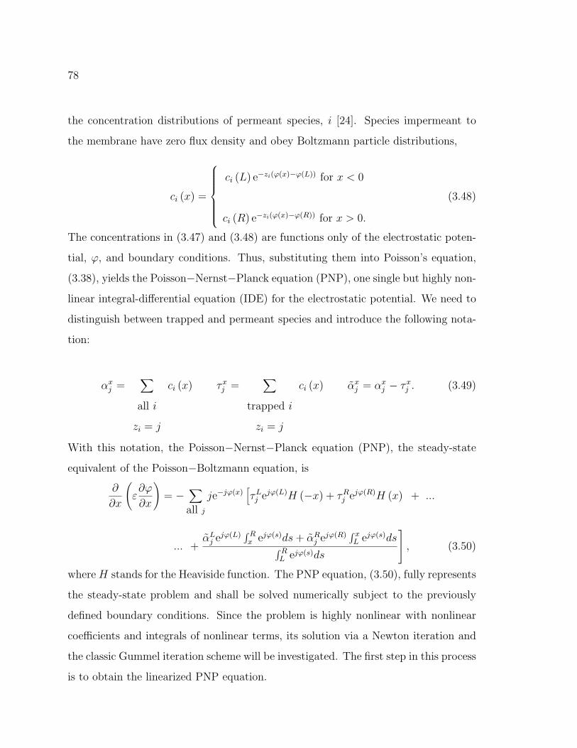
78
the concentration distributions of permeant species, i [24]. Species impermeant to
the membrane have zero flux density and obey Boltzmann particle distributions,
ci (x) =
ci (L) e−zi(ϕ(x)−ϕ(L)) for x < 0
ci (R) e−zi(ϕ(x)−ϕ(R)) for x > 0.
(3.48)
The concentrations in (3.47) and (3.48) are functions only of the electrostatic poten-
tial, ϕ, and boundary conditions. Thus, substituting them into Poisson’s equation,
(3.38), yields the Poisson−Nernst−Planck equation (PNP), one single but highly non-
linear integral-differential equation (IDE) for the electrostatic potential. We need to
distinguish between trapped and permeant species and introduce the following nota-
tion:
αxj =
∑all i
zi = j
ci (x) τxj =
∑trapped i
zi = j
ci (x) αxj = αx
j − τxj . (3.49)
With this notation, the Poisson−Nernst−Planck equation (PNP), the steady-state
equivalent of the Poisson−Boltzmann equation, is
∂
∂x
(ε∂ϕ
∂x
)= −
∑all j
je−jϕ(x)[τLj ejϕ(L)H (−x) + τR
j ejϕ(R)H (x) + ...
... +αL
j ejϕ(L)∫ Rx ejϕ(s)ds + αR
j ejϕ(R)∫ xL ejϕ(s)ds∫ R
L ejϕ(s)ds
, (3.50)
where H stands for the Heaviside function. The PNP equation, (3.50), fully represents
the steady-state problem and shall be solved numerically subject to the previously
defined boundary conditions. Since the problem is highly nonlinear with nonlinear
coefficients and integrals of nonlinear terms, its solution via a Newton iteration and
the classic Gummel iteration scheme will be investigated. The first step in this process
is to obtain the linearized PNP equation.
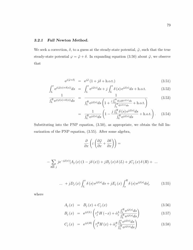
79
3.2.1 Full Newton Method.
We seek a correction, δ, to a guess at the steady-state potential, ϕ, such that the true
steady-state potential ϕ = ϕ + δ. In expanding equation (3.50) about ϕ, we observe
that
ej(ϕ+δ) = ejϕ (1 + jδ + h.o.t.) (3.51)∫ x
Lej(ϕ(s)+δ(s))ds =
∫ x
Lejϕ(s)ds + j
∫ x
Lδ (s) ejϕ(s)ds + h.o.t. (3.52)
1∫ RL ej(ϕ(s)+δ(s))ds
=1∫ R
L ejϕ(s)ds
(1 +
j∫ R
Lδ(s)ejϕ(s)ds∫ R
Lejϕ(s)ds
+ h.o.t.
) (3.53)
=1∫ R
L ejϕ(s)ds
(1− j
∫ RL δ (s) ejϕ(s)ds∫ R
L ejϕ(s)ds+ h.o.t.
). (3.54)
Substituting into the PNP equation, (3.50), as appropriate, we obtain the full lin-
earization of the PNP equation, (3.55). After some algebra,
∂
∂x
(ε
(∂ϕ
∂x+
∂δ
∂x
))=
−∑all j
je−jϕ(x)[Aj (x) (1− jδ (x)) + jBj (x) δ (L) + jCj (x) δ (R) + ...
... + jDj (x)∫ x
Lδ (s) ejϕ(s)ds + jEj (x)
∫ R
xδ (s) ejϕ(s)ds], (3.55)
where
Aj (x) = Bj (x) + Cj (x) (3.56)
Bj (x) = ejϕ(L)
(τLj H (−x) + αL
j
∫ Rx ejϕ(s)ds∫ RL ejϕ(s)ds
)(3.57)
Cj (x) = ejϕ(R)
(τRj H (x) + αR
j
∫ xL ejϕ(s)ds∫ RL ejϕ(s)ds
)(3.58)
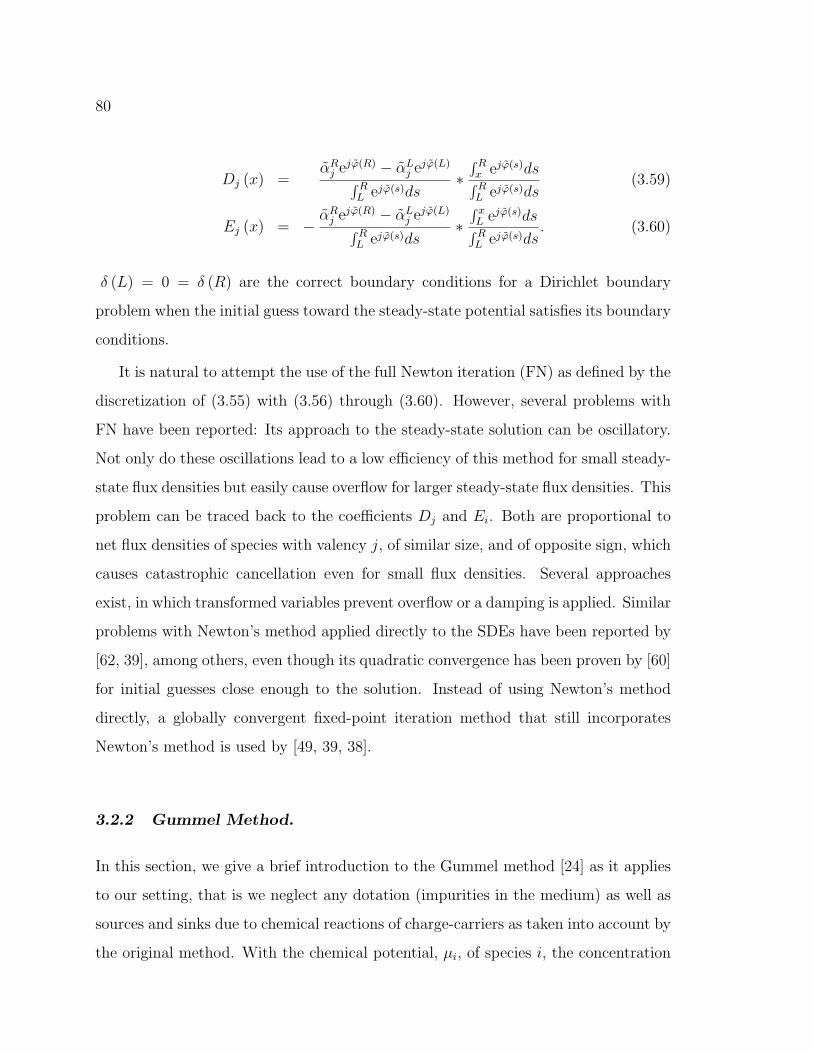
80
Dj (x) =αR
j ejϕ(R) − αLj ejϕ(L)∫ R
L ejϕ(s)ds∗∫ Rx ejϕ(s)ds∫ RL ejϕ(s)ds
(3.59)
Ej (x) = −αR
j ejϕ(R) − αLj ejϕ(L)∫ R
L ejϕ(s)ds∗∫ xL ejϕ(s)ds∫ RL ejϕ(s)ds
. (3.60)
δ (L) = 0 = δ (R) are the correct boundary conditions for a Dirichlet boundary
problem when the initial guess toward the steady-state potential satisfies its boundary
conditions.
It is natural to attempt the use of the full Newton iteration (FN) as defined by the
discretization of (3.55) with (3.56) through (3.60). However, several problems with
FN have been reported: Its approach to the steady-state solution can be oscillatory.
Not only do these oscillations lead to a low efficiency of this method for small steady-
state flux densities but easily cause overflow for larger steady-state flux densities. This
problem can be traced back to the coefficients Dj and Ei. Both are proportional to
net flux densities of species with valency j, of similar size, and of opposite sign, which
causes catastrophic cancellation even for small flux densities. Several approaches
exist, in which transformed variables prevent overflow or a damping is applied. Similar
problems with Newton’s method applied directly to the SDEs have been reported by
[62, 39], among others, even though its quadratic convergence has been proven by [60]
for initial guesses close enough to the solution. Instead of using Newton’s method
directly, a globally convergent fixed-point iteration method that still incorporates
Newton’s method is used by [49, 39, 38].
3.2.2 Gummel Method.
In this section, we give a brief introduction to the Gummel method [24] as it applies
to our setting, that is we neglect any dotation (impurities in the medium) as well as
sources and sinks due to chemical reactions of charge-carriers as taken into account by
the original method. With the chemical potential, µi, of species i, the concentration
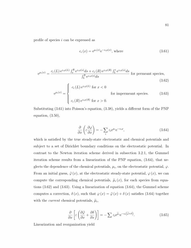
81
profile of species i can be expressed as
ci (x) = eµi(x)e−ziϕ(x), where (3.61)
eµi(x) =ci (L) eziϕ(L)
∫ Rx eziϕ(s)ds + ci (R) eziϕ(R)
∫ xL eziϕ(s)ds∫ R
L eziϕ(s)dsfor permeant species,
(3.62)
eµi(x) =
ci (L) eziϕ(L) for x < 0
ci (R) eziϕ(R) for x > 0.
for impermeant species. (3.63)
Substituting (3.61) into Poisson’s equation, (3.38), yields a different form of the PNP
equation, (3.50),
∂
∂x
(ε∂ϕ
∂x
)= −
∑i
zieµie−ziϕ, (3.64)
which is satisfied by the true steady-state electrostatic and chemical potentials and
subject to a set of Dirichlet boundary conditions on the electrostatic potential. In
contrast to the Newton iteration scheme derived in subsection 3.2.1, the Gummel
iteration scheme results from a linearization of the PNP equation, (3.64), that ne-
glects the dependence of the chemical potentials, µi, on the electrostatic potential, ϕ.
From an initial guess, ϕ (x), at the electrostatic steady-state potential, ϕ (x), we can
compute the corresponding chemical potentials, µi (x), for each species from equa-
tions (3.62) and (3.63). Using a linearization of equation (3.64), the Gummel scheme
computes a correction, δ (x), such that ϕ (x) = ϕ (x) + δ (x) satisfies (3.64) together
with the current chemical potentials, µi,
∂
∂x
[ε
(∂ϕ
∂x+
∂δ
∂x
)]= −
∑zie
µie−zi(ϕ+δ). (3.65)
Linearization and reorganization yield

82
∂
∂x
(ε∂δ
∂x
)−(∑
z2i e
µie−ziϕ)δ = − ∂
∂x
(ε∂ϕ
∂x
)−∑
zieµie−ziϕ, (3.66)
a linear differential equation for δ that satisfies zero boundary conditions, provided the
initial guess for the electro-static potential satisfies its Dirichlet boundary conditions.
Discretizing equation (3.66), solving the resulting system for δ, and taking ϕ = ϕ + δ
as the next guess at the steady-state potential creates an iterative method, namely
the Gummel method [24].
The dependence of the chemical potentials, µi, on ϕ throughout the domain has
been entirely neglected when linearizing (3.64). Due to this neglect, a difference
between the full Newton and Gummel schemes is expected and shall be explored. It
is easily verified that, for Dj (x) = 0 = Ej (x) and δ (L) = 0 = δ (R), the full Newton
method, as defined by (3.55), reduces to the equation defining the Gummel method,
(3.66). In other terms, the classic Gummel method is defined by (3.55) with coefficient
(3.56) only and Bj (x) through Ej (x) replaced by zero. The resulting discretization
is sparse, tri-diagonal, and thus efficiently solved. Because both Dj (x) and Ej (x) are
proportional to the net flux density of particle species with valency j, their neglect
may eliminate problems due to catastrophic cancellation as encountered by the full
Newton scheme. However, if flux densities become large, important contributions by
terms containing Dj (x) and Ej (x) are neglected and the Gummel method is expected
to converge less efficiently.
As a modified Gummel method (MG), we propose the method closest to the
original Gummel method that is capable of solving equation (3.64) subject to the
Dirichlet-Neumann boundary conditions, (3.41) or (3.42). That is, the modified
Gummel method is defined by (3.55) with coefficients (3.56) through (3.58) and
Dj (x) and Ej (x) replaced by zero. The resulting discretization is sparse, almost
tri-diagonal, thus efficiently solved, and encounters the same potential problems as
the original Gummel method.
It is, a priori, not clear whether the Gummel or modified Gummel method should
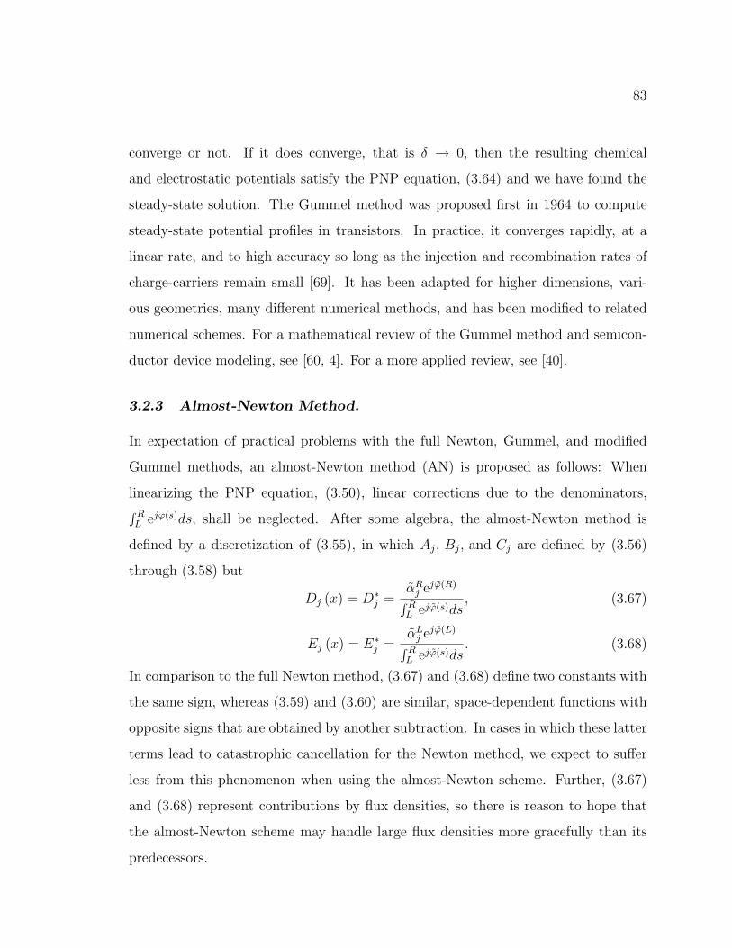
83
converge or not. If it does converge, that is δ → 0, then the resulting chemical
and electrostatic potentials satisfy the PNP equation, (3.64) and we have found the
steady-state solution. The Gummel method was proposed first in 1964 to compute
steady-state potential profiles in transistors. In practice, it converges rapidly, at a
linear rate, and to high accuracy so long as the injection and recombination rates of
charge-carriers remain small [69]. It has been adapted for higher dimensions, vari-
ous geometries, many different numerical methods, and has been modified to related
numerical schemes. For a mathematical review of the Gummel method and semicon-
ductor device modeling, see [60, 4]. For a more applied review, see [40].
3.2.3 Almost-Newton Method.
In expectation of practical problems with the full Newton, Gummel, and modified
Gummel methods, an almost-Newton method (AN) is proposed as follows: When
linearizing the PNP equation, (3.50), linear corrections due to the denominators,∫ RL ejϕ(s)ds, shall be neglected. After some algebra, the almost-Newton method is
defined by a discretization of (3.55), in which Aj, Bj, and Cj are defined by (3.56)
through (3.58) but
Dj (x) = D∗j =
αRj ejϕ(R)∫ R
L ejϕ(s)ds, (3.67)
Ej (x) = E∗j =
αLj ejϕ(L)∫ R
L ejϕ(s)ds. (3.68)
In comparison to the full Newton method, (3.67) and (3.68) define two constants with
the same sign, whereas (3.59) and (3.60) are similar, space-dependent functions with
opposite signs that are obtained by another subtraction. In cases in which these latter
terms lead to catastrophic cancellation for the Newton method, we expect to suffer
less from this phenomenon when using the almost-Newton scheme. Further, (3.67)
and (3.68) represent contributions by flux densities, so there is reason to hope that
the almost-Newton scheme may handle large flux densities more gracefully than its
predecessors.
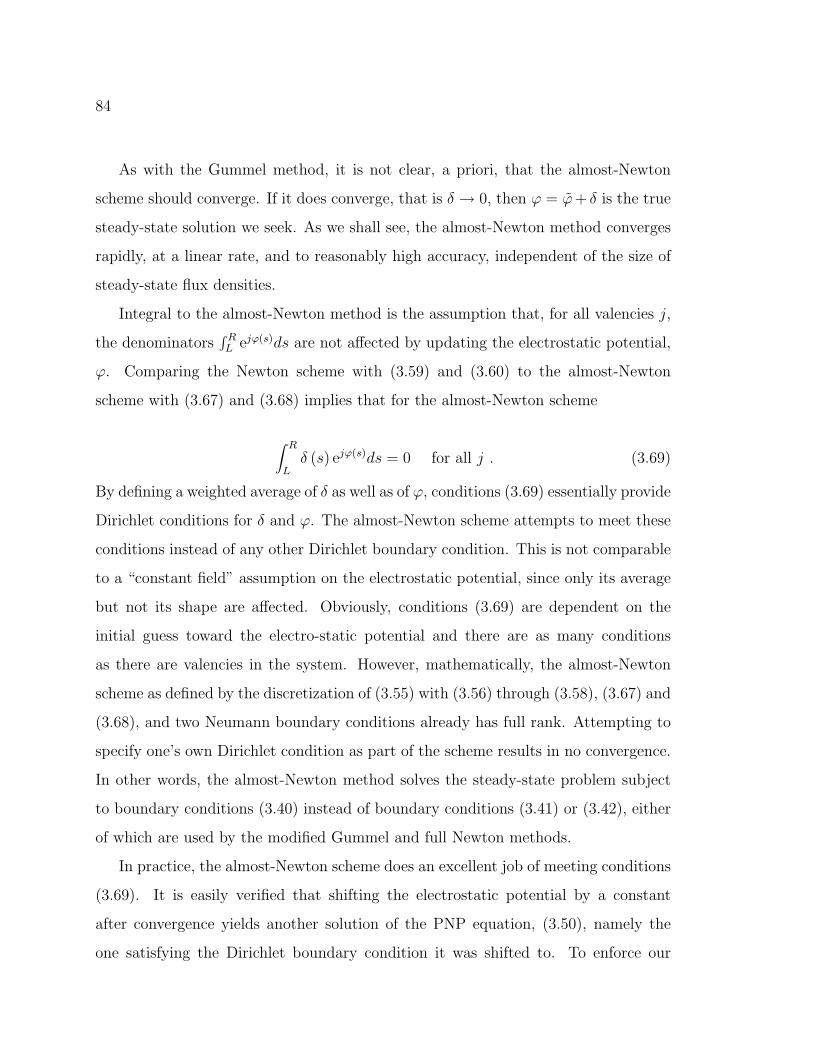
84
As with the Gummel method, it is not clear, a priori, that the almost-Newton
scheme should converge. If it does converge, that is δ → 0, then ϕ = ϕ+ δ is the true
steady-state solution we seek. As we shall see, the almost-Newton method converges
rapidly, at a linear rate, and to reasonably high accuracy, independent of the size of
steady-state flux densities.
Integral to the almost-Newton method is the assumption that, for all valencies j,
the denominators∫ RL ejϕ(s)ds are not affected by updating the electrostatic potential,
ϕ. Comparing the Newton scheme with (3.59) and (3.60) to the almost-Newton
scheme with (3.67) and (3.68) implies that for the almost-Newton scheme
∫ R
Lδ (s) ejϕ(s)ds = 0 for all j . (3.69)
By defining a weighted average of δ as well as of ϕ, conditions (3.69) essentially provide
Dirichlet conditions for δ and ϕ. The almost-Newton scheme attempts to meet these
conditions instead of any other Dirichlet boundary condition. This is not comparable
to a “constant field” assumption on the electrostatic potential, since only its average
but not its shape are affected. Obviously, conditions (3.69) are dependent on the
initial guess toward the electro-static potential and there are as many conditions
as there are valencies in the system. However, mathematically, the almost-Newton
scheme as defined by the discretization of (3.55) with (3.56) through (3.58), (3.67) and
(3.68), and two Neumann boundary conditions already has full rank. Attempting to
specify one’s own Dirichlet condition as part of the scheme results in no convergence.
In other words, the almost-Newton method solves the steady-state problem subject
to boundary conditions (3.40) instead of boundary conditions (3.41) or (3.42), either
of which are used by the modified Gummel and full Newton methods.
In practice, the almost-Newton scheme does an excellent job of meeting conditions
(3.69). It is easily verified that shifting the electrostatic potential by a constant
after convergence yields another solution of the PNP equation, (3.50), namely the
one satisfying the Dirichlet boundary condition it was shifted to. To enforce our
85
Dirichlet condition of choice when using the almost-Newton method, we thus shift
the electrostatic potential by the appropriate constant after convergence.
3.2.4 Comparison of Iterative Methods.
We consider a monovalent case, in which the system contains ions of sodium (Na),
chloride (Cl), and a large protein (P). The protein carries one negative elementary
charge and is confined by the semi-permeable membrane to the left (internal) side of
the domain at a concentration of 1 mmol/L. Different steady-states are investigated
by keeping the total mass in the system fixed and keeping bulk compartments electro-
neutral while varying the internal Cl concentration. In particular, we hold the internal
Cl bulk concentration at different values ranging from 20 mmol/L to 170 mmol/L. As a
result of keeping the total mass constant in the bulk of the system, the external Cl bulk
concentration ranges from 620 mmol/L to 20 mmol/L and the flux densities relative
to their respective diffusion coefficients range from -80 fmol/µm4 to 20 fmol/µm4.
Na concentrations in the bulk are fixed at values ensuring bulk electro-neutrality.
For all shown computations, the initial guess toward the electrostatic potential is
ϕ (x) = 0. We compare all three methods, modified Gummel (MG), full Newton (FN),
and almost-Newton (AN), with respect to their accuracy and number of iteration steps
they need to converge. In cases where no analytic solution is available, the solution
obtained by FN subject to boundary conditions (3.42) is used as reference.
The most important performance indicator to observe is the error in the numeri-
cal solutions. At equilibrium, we compute errors directly from an available analytic
solution. In figure 3.2, we show the results of a grid-refinement study of MG, AN,
and FN at equilibrium. In particular, we show on the left of figure 3.2 the absolute
relative error in the cross-membrane potential difference, ϕ (R) − ϕ (L), at conver-
gence of MG, FN, and AN. At any given resolution, all three methods commit very
similar errors which, in fact, cannot be distinguished by the naked eye. From a
closer investigation not shown here, we find that a resolution of about 100 grid points

86
Figure 3.2: Various grid resolutions at equilibrium. Left: Absolute value of relative
error in cross-membrane potential difference. Right: Maximum absolute residual.
throughout the domain is optimal for all methods in the sense that for smaller as well
as higher resolutions, a larger error is committed. This phenomenon is well known
in numerical analysis: While the larger error below 100 grid points is dominated by
the discretization error, the error increase beyond 100 grid points is dominated by
round-off error.
Another important indicator for how well each method approximates the solution
of the PNP equation, (3.50), is its residual. On the right of figure 3.2, we show
further results of the grid-refinement study at equilibrium for MG, AN, and FN. In
particular, we show the maximum absolute size of the residual at convergence of each
method. The residual of MG is almost the same as that of FN. The residual of AN is
consistently larger than that of FN but small enough to consider a solution obtained
by AN a solution of the PNP equation, (3.50). This does not come as a surprise
because AN uses an approximation of the true Jacobian of the system to solve the
problem and thus, can only approach the true solution within the space accessible to
this approximation.
Next, we compare MG, FN, and AN with respect to the number of iteration steps
they need to converge. We explore various steady-states as characterized by their
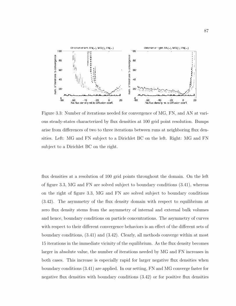
87
Figure 3.3: Number of iterations needed for convergence of MG, FN, and AN at vari-
ous steady-states characterized by flux densities at 100 grid point resolution. Bumps
arise from differences of two to three iterations between runs at neighboring flux den-
sities. Left: MG and FN subject to a Dirichlet BC on the left. Right: MG and FN
subject to a Dirichlet BC on the right.
flux densities at a resolution of 100 grid points throughout the domain. On the left
of figure 3.3, MG and FN are solved subject to boundary conditions (3.41), whereas
on the right of figure 3.3, MG and FN are solved subject to boundary conditions
(3.42). The asymmetry of the flux density domain with respect to equilibrium at
zero flux density stems from the asymmetry of internal and external bulk volumes
and hence, boundary conditions on particle concentrations. The asymmetry of curves
with respect to their different convergence behaviors is an effect of the different sets of
boundary conditions, (3.41) and (3.42). Clearly, all methods converge within at most
15 iterations in the immediate vicinity of the equilibrium. As the flux density becomes
larger in absolute value, the number of iterations needed by MG and FN increases in
both cases. This increase is especially rapid for larger negative flux densities when
boundary conditions (3.41) are applied. In our setting, FN and MG converge faster for
negative flux densities with boundary conditions (3.42) or for positive flux densities
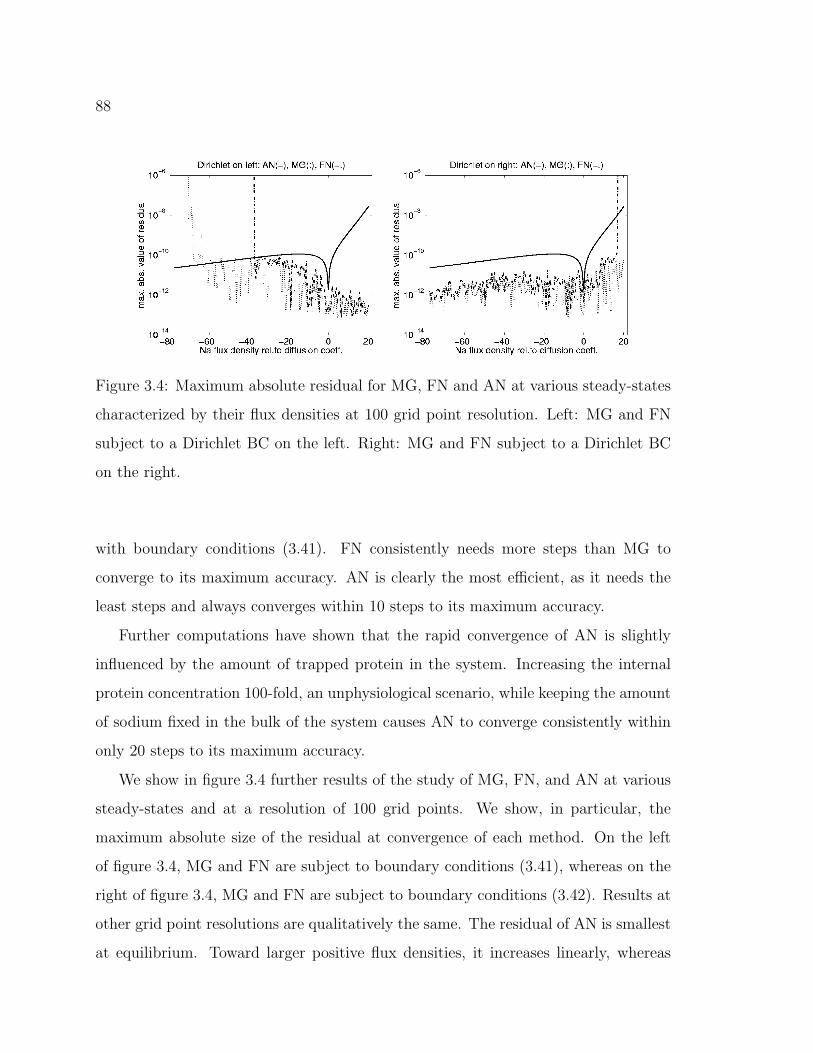
88
Figure 3.4: Maximum absolute residual for MG, FN and AN at various steady-states
characterized by their flux densities at 100 grid point resolution. Left: MG and FN
subject to a Dirichlet BC on the left. Right: MG and FN subject to a Dirichlet BC
on the right.
with boundary conditions (3.41). FN consistently needs more steps than MG to
converge to its maximum accuracy. AN is clearly the most efficient, as it needs the
least steps and always converges within 10 steps to its maximum accuracy.
Further computations have shown that the rapid convergence of AN is slightly
influenced by the amount of trapped protein in the system. Increasing the internal
protein concentration 100-fold, an unphysiological scenario, while keeping the amount
of sodium fixed in the bulk of the system causes AN to converge consistently within
only 20 steps to its maximum accuracy.
We show in figure 3.4 further results of the study of MG, FN, and AN at various
steady-states and at a resolution of 100 grid points. We show, in particular, the
maximum absolute size of the residual at convergence of each method. On the left
of figure 3.4, MG and FN are subject to boundary conditions (3.41), whereas on the
right of figure 3.4, MG and FN are subject to boundary conditions (3.42). Results at
other grid point resolutions are qualitatively the same. The residual of AN is smallest
at equilibrium. Toward larger positive flux densities, it increases linearly, whereas
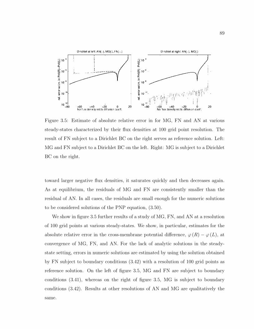
89
Figure 3.5: Estimate of absolute relative error in for MG, FN and AN at various
steady-states characterized by their flux densities at 100 grid point resolution. The
result of FN subject to a Dirichlet BC on the right serves as reference solution. Left:
MG and FN subject to a Dirichlet BC on the left. Right: MG is subject to a Dirichlet
BC on the right.
toward larger negative flux densities, it saturates quickly and then decreases again.
As at equilibrium, the residuals of MG and FN are consistently smaller than the
residual of AN. In all cases, the residuals are small enough for the numeric solutions
to be considered solutions of the PNP equation, (3.50).
We show in figure 3.5 further results of a study of MG, FN, and AN at a resolution
of 100 grid points at various steady-states. We show, in particular, estimates for the
absolute relative error in the cross-membrane potential difference, ϕ (R) − ϕ (L), at
convergence of MG, FN, and AN. For the lack of analytic solutions in the steady-
state setting, errors in numeric solutions are estimated by using the solution obtained
by FN subject to boundary conditions (3.42) with a resolution of 100 grid points as
reference solution. On the left of figure 3.5, MG and FN are subject to boundary
conditions (3.41), whereas on the right of figure 3.5, MG is subject to boundary
conditions (3.42). Results at other resolutions of AN and MG are qualitatively the
same.
90
From both plots in figure 3.5, we see that, given a set of boundary conditions,
MG and FN compute almost the same potential difference across the domain. This
is expected because FN and MG solve the same mathematical problem. As seen on
the left of figure 3.5, potential differences computed with boundary conditions (3.41)
show a relative difference of about O (10−6) to the reference for larger negative flux
densities. This is the same as the accuracy observed at equilibrium for the considered
resolution (figure 3.2) and may thus serve as an estimate for the accuracy of MG and
FN for larger negative flux densities. For larger positive flux densities, the error MG
and FN commit to the reference increases almost linearly from O (10−6) to O (10−4),
and may serve as an estimate for the accuracy of MG and FN for larger positive flux
densities. With boundary conditions (3.41), AN is consistently closer to the reference
solution than MG or FN and thus lies in between their solutions subject to the two
arbitrary sets of boundary conditions, (3.41) and (3.42). Given these considerations,
AN is concluded to be at least as accurate as MG or FN.
Another advantage of AN over MG and FN besides its rapid convergence and com-
parable accuracy is that there is no ambiguity in the choice of boundary conditions.
AN solves the PNP equation, (3.50), subject to the initially derived, natural set of
boundary conditions, (3.40), based upon Gauss’ law. This set of boundary conditions
usually does not lead to a mathematically well-posed problem for lack of a Dirichlet
condition. It can only be used successfully when applying a method like AN that pro-
vides its own Dirichlet condition. When solving (3.50) with MG or FN, the conditions
(3.40) need to be replaced by either (3.41) or (3.42) to define a well-posed problem.
However, all three sets of conditions define problems which are mathematically dif-
ferent from each other, and therefore difficult to compare. More importantly, when
using MG or FN with mathematically appropriate boundary conditions, a slightly
different problem is solved compared to the one that was originally intended to be
solved. Further, the efficient use of either MG or FN requires a means of predicting
a method’s preferred boundary condition. This seems easy in our current setting but
91
may become complicated with more species and valencies involved, especially with
multiple trapped protein species. For all the above reasons, AN shall be used for
solving (3.50) subject to (3.40) and for doing so efficiently.
3.3 Numeric Simulation of the Quasi Steady-State Approx-
imation
Consider the well-posed system of PDEs (3.70) with differential operators L1,2, and
small parameter ε 1 after normalization and non-dimensionalization,
εxt = L1 (x, y)
yt = L2 (x, y) .(3.70)
The relatively slow dynamics of y may be approximated by neglecting the small term
εxt in (3.70), obtaining
0 = L1 (x, y)
yt = L2 (x, y) .(3.71)
This is equivalent to assuming that x has reached its steady state associated with
y. While y obeys its dynamics governed by L2, x passes through its corresponding,
consecutive steady-states. Since the original problem is well-posed, the first equation
in (3.71) can be solved for x while treating y as a parameter. The result should
technically be x = l1 (y), such that y obeys the quasi steady-state approximation
(QSSA),
yt = L2 (l1 (y) , y) . (3.72)
However, problems may arise if l1 (y) is multi-valued. One then needs criteria by
which to decide which one of multiple states x is appropriate to choose. It is also
often not possible to solve for x in terms of y explicitly. In this latter case, one
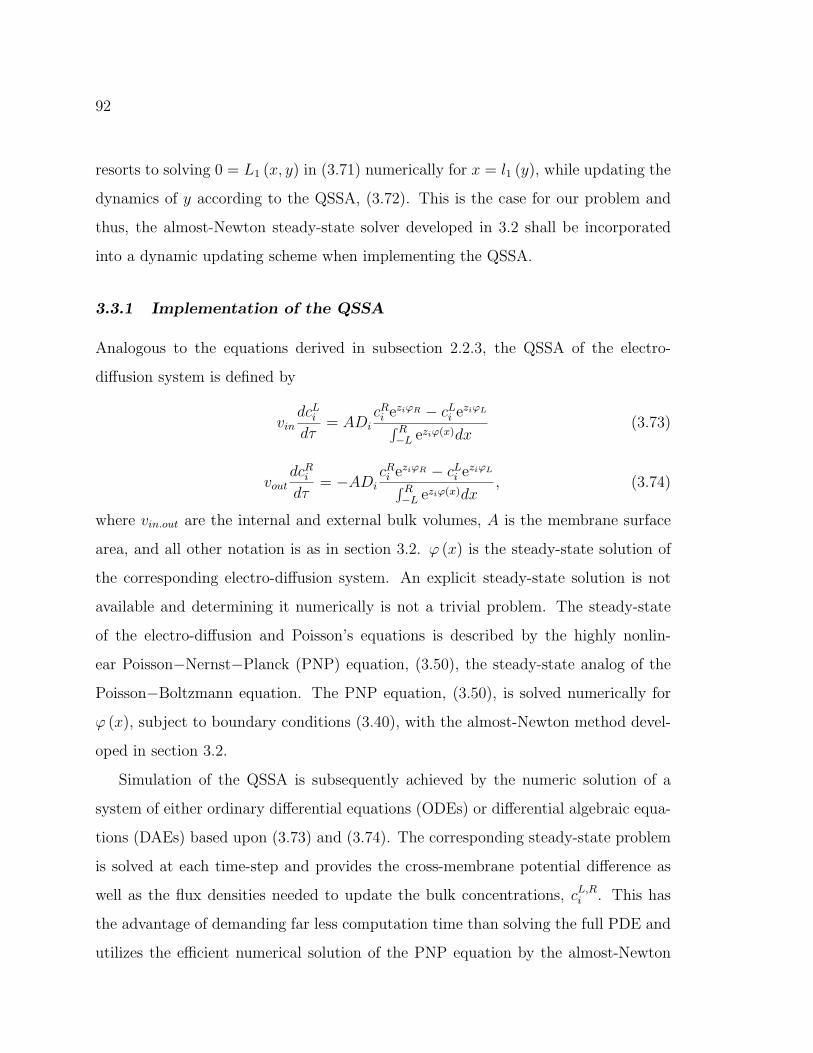
92
resorts to solving 0 = L1 (x, y) in (3.71) numerically for x = l1 (y), while updating the
dynamics of y according to the QSSA, (3.72). This is the case for our problem and
thus, the almost-Newton steady-state solver developed in 3.2 shall be incorporated
into a dynamic updating scheme when implementing the QSSA.
3.3.1 Implementation of the QSSA
Analogous to the equations derived in subsection 2.2.3, the QSSA of the electro-
diffusion system is defined by
vindcL
i
dτ= ADi
cRi eziϕR − cL
i eziϕL∫ R−L eziϕ(x)dx
(3.73)
voutdcR
i
dτ= −ADi
cRi eziϕR − cL
i eziϕL∫ R−L eziϕ(x)dx
, (3.74)
where vin.out are the internal and external bulk volumes, A is the membrane surface
area, and all other notation is as in section 3.2. ϕ (x) is the steady-state solution of
the corresponding electro-diffusion system. An explicit steady-state solution is not
available and determining it numerically is not a trivial problem. The steady-state
of the electro-diffusion and Poisson’s equations is described by the highly nonlin-
ear Poisson−Nernst−Planck (PNP) equation, (3.50), the steady-state analog of the
Poisson−Boltzmann equation. The PNP equation, (3.50), is solved numerically for
ϕ (x), subject to boundary conditions (3.40), with the almost-Newton method devel-
oped in section 3.2.
Simulation of the QSSA is subsequently achieved by the numeric solution of a
system of either ordinary differential equations (ODEs) or differential algebraic equa-
tions (DAEs) based upon (3.73) and (3.74). The corresponding steady-state problem
is solved at each time-step and provides the cross-membrane potential difference as
well as the flux densities needed to update the bulk concentrations, cL,Ri . This has
the advantage of demanding far less computation time than solving the full PDE and
utilizes the efficient numerical solution of the PNP equation by the almost-Newton
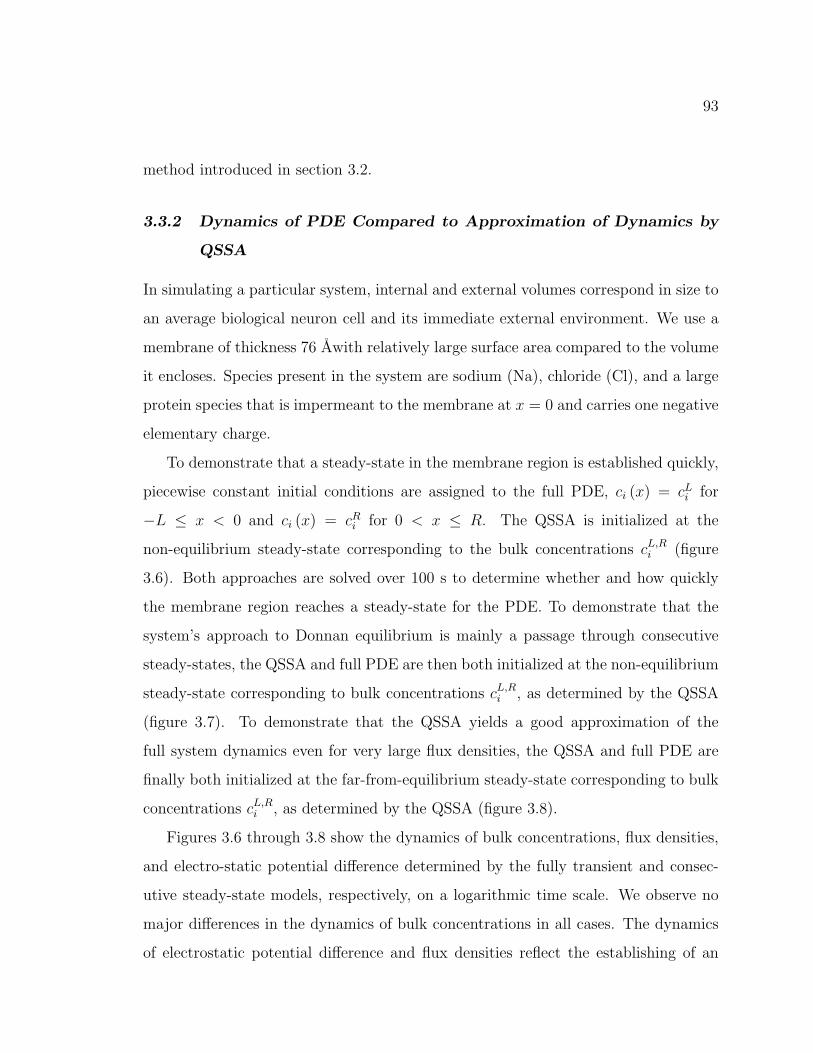
93
method introduced in section 3.2.
3.3.2 Dynamics of PDE Compared to Approximation of Dynamics by
QSSA
In simulating a particular system, internal and external volumes correspond in size to
an average biological neuron cell and its immediate external environment. We use a
membrane of thickness 76 Awith relatively large surface area compared to the volume
it encloses. Species present in the system are sodium (Na), chloride (Cl), and a large
protein species that is impermeant to the membrane at x = 0 and carries one negative
elementary charge.
To demonstrate that a steady-state in the membrane region is established quickly,
piecewise constant initial conditions are assigned to the full PDE, ci (x) = cLi for
−L ≤ x < 0 and ci (x) = cRi for 0 < x ≤ R. The QSSA is initialized at the
non-equilibrium steady-state corresponding to the bulk concentrations cL,Ri (figure
3.6). Both approaches are solved over 100 s to determine whether and how quickly
the membrane region reaches a steady-state for the PDE. To demonstrate that the
system’s approach to Donnan equilibrium is mainly a passage through consecutive
steady-states, the QSSA and full PDE are then both initialized at the non-equilibrium
steady-state corresponding to bulk concentrations cL,Ri , as determined by the QSSA
(figure 3.7). To demonstrate that the QSSA yields a good approximation of the
full system dynamics even for very large flux densities, the QSSA and full PDE are
finally both initialized at the far-from-equilibrium steady-state corresponding to bulk
concentrations cL,Ri , as determined by the QSSA (figure 3.8).
Figures 3.6 through 3.8 show the dynamics of bulk concentrations, flux densities,
and electro-static potential difference determined by the fully transient and consec-
utive steady-state models, respectively, on a logarithmic time scale. We observe no
major differences in the dynamics of bulk concentrations in all cases. The dynamics
of electrostatic potential difference and flux densities reflect the establishing of an
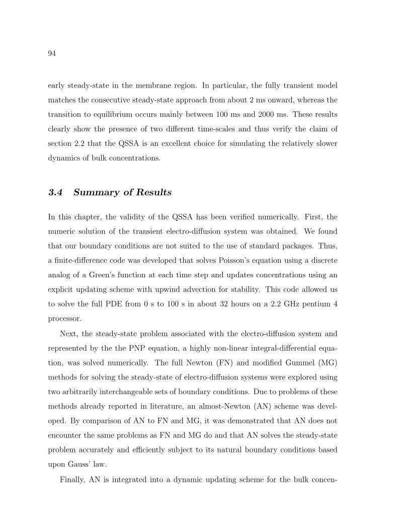
94
early steady-state in the membrane region. In particular, the fully transient model
matches the consecutive steady-state approach from about 2 ms onward, whereas the
transition to equilibrium occurs mainly between 100 ms and 2000 ms. These results
clearly show the presence of two different time-scales and thus verify the claim of
section 2.2 that the QSSA is an excellent choice for simulating the relatively slower
dynamics of bulk concentrations.
3.4 Summary of Results
In this chapter, the validity of the QSSA has been verified numerically. First, the
numeric solution of the transient electro-diffusion system was obtained. We found
that our boundary conditions are not suited to the use of standard packages. Thus,
a finite-difference code was developed that solves Poisson’s equation using a discrete
analog of a Green’s function at each time step and updates concentrations using an
explicit updating scheme with upwind advection for stability. This code allowed us
to solve the full PDE from 0 s to 100 s in about 32 hours on a 2.2 GHz pentium 4
processor.
Next, the steady-state problem associated with the electro-diffusion system and
represented by the the PNP equation, a highly non-linear integral-differential equa-
tion, was solved numerically. The full Newton (FN) and modified Gummel (MG)
methods for solving the steady-state of electro-diffusion systems were explored using
two arbitrarily interchangeable sets of boundary conditions. Due to problems of these
methods already reported in literature, an almost-Newton (AN) scheme was devel-
oped. By comparison of AN to FN and MG, it was demonstrated that AN does not
encounter the same problems as FN and MG do and that AN solves the steady-state
problem accurately and efficiently subject to its natural boundary conditions based
upon Gauss’ law.
Finally, AN is integrated into a dynamic updating scheme for the bulk concen-
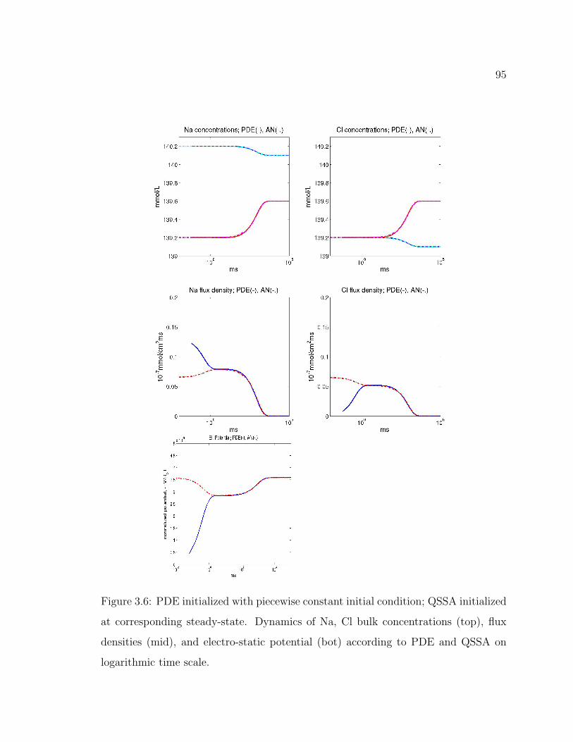
95
Figure 3.6: PDE initialized with piecewise constant initial condition; QSSA initialized
at corresponding steady-state. Dynamics of Na, Cl bulk concentrations (top), flux
densities (mid), and electro-static potential (bot) according to PDE and QSSA on
logarithmic time scale.
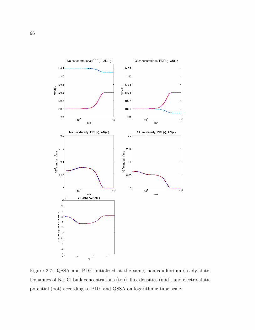
96
Figure 3.7: QSSA and PDE initialized at the same, non-equilibrium steady-state.
Dynamics of Na, Cl bulk concentrations (top), flux densities (mid), and electro-static
potential (bot) according to PDE and QSSA on logarithmic time scale.

97
Figure 3.8: QSSA and PDE initialized at the same, far-from-equilibrium steady-state.
Dynamics of Na, Cl bulk concentrations (top), flux densities (mid), and electro-static
potential (bot) according to PDE and QSSA on logarithmic time scale.
98
trations to implement the quasi steady-state approximation (QSSA) of the electro-
diffusion system. This code allowed us to simulate the QSSA from 0 s to 100 s in
about 10 minutes on a 2.2 GHz pentium 4 processor. It was demonstrated for three
sets of initial conditions that a separation of time scales occurs as claimed and that
the dynamics of the QSSA compare well with those of the transient PDE. Clearly, the
implementation of the QSSA provides not only an accurate but also a highly efficient
means of approximating the dynamics of our electro-diffusion system.
99
Chapter 4
FROM QSSA TO THE CLASSIC HODGKIN−HUXLEY
MODEL
In subsection 2.1.1, the location of zero flux for impermeant species was discussed
and put at mid-membrane, x = 0. This allowed results of the quasi steady-state
approximation (QSSA) to be compared to corresponding results of the fully transient
electro-diffusion system at a reasonable expense of computing time. It is my goal
in this chapter to compare the QSSA, which requires a steady-state problem to be
solved at each time step, to two approximations of the QSSA that are described
by systems of ordinary differential equations (ODEs). The first approximation of
the QSSA results from applying a GHK-like constant field assumption (CFA) to the
electro-static potential. The second approximation of the QSSA is its linearization
with respect to the electro-static potential that results in a Hodgkin−Huxley-like
model (HHplk).
Throughout this chapter, to be able to compare the QSSA to the CFA model, we
adopt the option discarded in subsection 2.1.1 that puts the zero-flux conditions for
impermeant species at the membrane boundaries, x = ±m2.
4.1 Adjusting to end-of-membrane impermeability
Enforcing zero-flux conditions on impermeant species at both ends of the membrane
results in the formation of a pair of boundary layers about each location of zero-flux,
x = ±m2. For each pair, one boundary layer lies in the membrane region and the other
one in the bulk. It is understood that all boundary layers have to be included in the
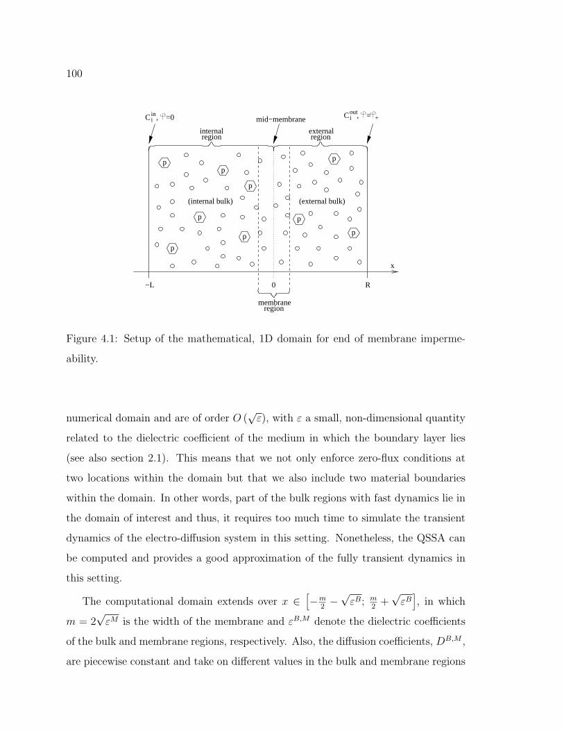
100
region regionexternalinternal
membraneregion
−L 0 R
x
p
p
p
p
p
C , =0iin C , =i
out+mid−membrane
p
(internal bulk) (external bulk)
p
p
p
Figure 4.1: Setup of the mathematical, 1D domain for end of membrane imperme-
ability.
numerical domain and are of order O (√
ε), with ε a small, non-dimensional quantity
related to the dielectric coefficient of the medium in which the boundary layer lies
(see also section 2.1). This means that we not only enforce zero-flux conditions at
two locations within the domain but that we also include two material boundaries
within the domain. In other words, part of the bulk regions with fast dynamics lie in
the domain of interest and thus, it requires too much time to simulate the transient
dynamics of the electro-diffusion system in this setting. Nonetheless, the QSSA can
be computed and provides a good approximation of the fully transient dynamics in
this setting.
The computational domain extends over x ∈[−m
2−√
εB; m2
+√
εB], in which
m = 2√
εM is the width of the membrane and εB,M denote the dielectric coefficients
of the bulk and membrane regions, respectively. Also, the diffusion coefficients, DB,M ,
are piecewise constant and take on different values in the bulk and membrane regions
101
of the domain, respectively. Due to the fast dynamics in the bulk, the ion concentra-
tions at each end of the computational domain are ci (−L) and ci (R) for species i,
the constant bulk concentrations.
It is a well-known property of the electric field, ∇ϕ, that the normal component of
the dielectric displacement, ε∇ϕ, is continuous across dielectric material boundaries.
Thus,
εB dϕ
dx
(−m
2
−)= εM dϕ
dx
(−m
2
+)
(4.1)
εM dϕ
dx
(m
2
−)= εB dϕ
dx
(m
2
+)
. (4.2)
It is straightforward to adjust the QSSA for mid-membrane impermeability (QSSA-
mid) to the QSSA for end-of-membrane impermeability (QSSA-end) by implementing
the above changes. QSSA-end converges as quickly as QSSA-mid to its maximum
accuracy. On the other hand, the estimated accuracy to which QSSA-end converges is
lower than that of QSSA-mid. This is somewhat expected since QSSA-end deals with
large discontinuities of piecewise constant parameters within the domain, whereas
QSSA-mid deals only with constant parameters throughout its domain.
4.2 Constant field approximation of the QSSA
In the setting of end-of-membrane impermeability, any local net-charge accumulates
close to the material boundaries at x = ±m2. Since the entire two-compartment
system is electro-neutral, the net-charge around x = −m2
balances the net-charge
around x = m2. Consider the 1D Poisson equation in the form of Gauss’ law,
εdϕ
dx(x) = −
∫ x
L
∑i
zici (s) ds , (4.3)
102
where L = −m2−√
εB, the left end of the computational domain, and recall that, with
net electro-neutral bulk, dϕdx
(L) = 0. According to (4.3), the electric field, dϕdx
, at some
place x away from loci of charge accumulation is approximately constant and propor-
tional to the net-charge accumulated between L and x. Combining these observations
with system electro-neutrality implies that the electric field is approximately zero in
both bulk regions and proportional to the net-charge around x = m2
in the membrane
region of the domain. Assuming the charge accumulations around x = ±m2
occupy
relatively narrow pieces of the domain implies a piecewise linear approximation of the
electro-static potential.
Furthermore, since εM εB, any net-charge has a much larger effect on the
electric field in the membrane region than in the bulk region. Thus, it is expected
that the electro-static potential in the membrane region of the domain contributes
most to the cross-membrane potential difference. Its linear approximation should
therefore provide a qualitatively as well as quantitatively reasonable approximation
of both the electro-static potential profile and cross-membrane potential difference.
4.2.1 Derivation of the constant field approximation (CFA)
Let L = −m2−√
εB and R = m2
+√
εB be the ends of the computational domain.
Given net electro-neutral boundary values for ion concentrations of species i, ci (L)
and ci (R), the steady-state potential corresponding to the QSSA satisfy the PNP
equation, (3.50), which is equivalent to Poisson’s equation,
d
dx
(εdϕ
dx
)= −
∑i
zici , (4.4)
with the steady-state concentrations of permeant species,
ci (x) = e−ziϕ(x) ci (L) eziϕ(L)∫ Rx eziϕ(s)ds + ci (R) eziϕ(R)
∫ xL eziϕ(s)ds∫ R
L eziϕ(s)ds, (4.5)
and with impermeant species obeying Boltzmann particle distributions,
103
ci (x) =
ci (L) e−zi(ϕ(x)−ϕ(L)) for x < 0
ci (R) e−zi(ϕ(x)−ϕ(R)) for x > 0.
(4.6)
Our interest lies in the constant field approximation (CFA) of the electro-static po-
tential, ϕ, and flux densities, Ji, of permeant species,
Ji = −Dici (R) eziϕ(R) − ci (L) eziϕ(L)∫ R
L eziϕ(s)ds. (4.7)
According to (4.4),
εdϕ
dx(x) = −
∫ x
L
∑i
zici (s) ds , (4.8)
As a result, the electric field in the bulks and at mid-membrane can be expressed as
εBAcdϕ
dx(L) = 0 , (4.9)
εMAcdϕ
dx(0) = −vin
∑i
zicini , (4.10)
εBAcdϕ
dx(R) = −vin
∑i
zicini − vout
∑i
zicouti = 0 , (4.11)
where cin,outi denotes the average internal or external concentration of species i, Ac is
the membrane surface area, and vin,out are the volumes to either side of mid-membrane.
The corresponding CFA uses
dϕ
dx(x) =
0 , for x < −m
2
− vin
εMAc
∑i zic
ini , for − m
2≤ x ≤ m
2
0 , for m2
< x
(4.12)
to define the electro-static potential ϕ (x)− ϕ (L) =∫ xL
dϕds
ds, that is
104
ϕ (x)− ϕ (L) =
0 , for x < −m
2
−(x + m
2
)vin
εMAc
∑i zic
ini , for − m
2≤ x ≤ m
2
−m vin
εMAc
∑i zic
ini , for m
2< x .
(4.13)
In particular, the cross-membrane potential
ϕ (R)− ϕ (L) = ∆ϕ = −m vin
εMAc
∑i
zicini . (4.14)
With the such defined electro-static potential, the integral in the expression defining
the flux density, (4.7), can be computed and the flux density according to the CFA
can be written as
Ji = −Dizi (ϕ (R)− ϕ (L))
m· ci (R) eziϕ(R) − ci (L) eziϕ(L)
eziϕ(R) − eziϕ(L)(4.15)
= −Dizi∆ϕ
m· ci (R) ezi∆ϕ − ci (L)
ezi∆ϕ − 1(4.16)
= DiziFV
mR0T· ci (R) e
−ziFVR0T − ci (L)
e−zi
FVR0T − 1
(4.17)
≈ DiziFV
mR0T· cout
i e−zi
FVR0T − cin
i
e−zi
FVR0T − 1
, (4.18)
where we have approximated the true bulk concentrations by the average concentra-
tion in each compartment and
∆ϕ = − FV
R0T= −m vin
εMAc
∑i
zicini , (4.19)
with the absolute cross-membrane voltage, V , Faraday’s constant, F , the universal gas
constant, R0, and absolute temperature, T . It is understood that concentrations are
updated according to the continuity equation and mass conservation. The equations
describing the dynamics according to the CFA model are, in summary,
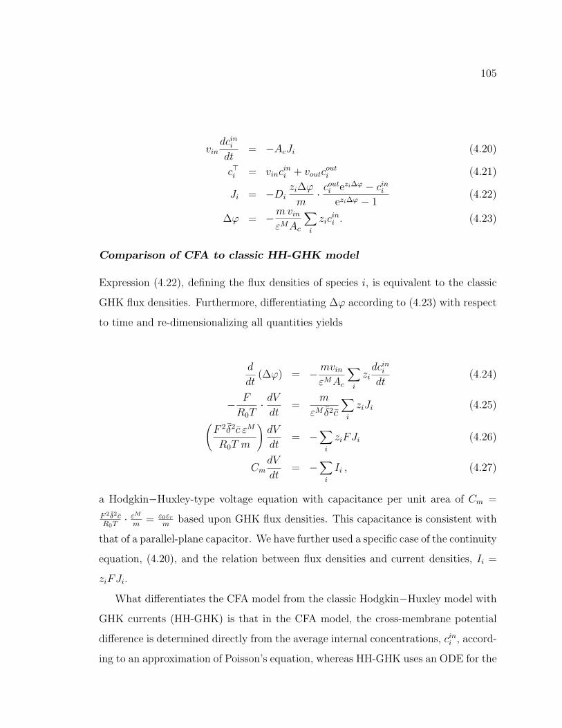
105
vindcin
i
dt= −AcJi (4.20)
c>i = vincini + voutc
outi (4.21)
Ji = −Dizi∆ϕ
m· cout
i ezi∆ϕ − cini
ezi∆ϕ − 1(4.22)
∆ϕ = −m vin
εMAc
∑i
zicini . (4.23)
Comparison of CFA to classic HH-GHK model
Expression (4.22), defining the flux densities of species i, is equivalent to the classic
GHK flux densities. Furthermore, differentiating ∆ϕ according to (4.23) with respect
to time and re-dimensionalizing all quantities yields
d
dt(∆ϕ) = −mvin
εMAc
∑i
zidcin
i
dt(4.24)
− F
R0T· dV
dt=
m
εM δ2c
∑i
ziJi (4.25)(F 2δ2c εM
R0T m
)dV
dt= −
∑i
ziFJi (4.26)
CmdV
dt= −
∑i
Ii , (4.27)
a Hodgkin−Huxley-type voltage equation with capacitance per unit area of Cm =
F 2δ2cR0T
· εM
m= ε0εr
mbased upon GHK flux densities. This capacitance is consistent with
that of a parallel-plane capacitor. We have further used a specific case of the continuity
equation, (4.20), and the relation between flux densities and current densities, Ii =
ziFJi.
What differentiates the CFA model from the classic Hodgkin−Huxley model with
GHK currents (HH-GHK) is that in the CFA model, the cross-membrane potential
difference is determined directly from the average internal concentrations, cini , accord-
ing to an approximation of Poisson’s equation, whereas HH-GHK uses an ODE for the
106
cross-membrane voltage based upon the current-voltage relationship in a model circuit
that includes a capacitor and multiple conductances (see also figure 1.10). Thus, the
CFA requires its bulk concentrations to be net electro-neutral and its average internal
concentrations to be close to net electro-neutral, whereas HH-GHK does not require
or consider electro-neutrality. Furthermore, the CFA models a closed, finite-volume,
two-compartment system in which concentrations obey conditions of mass conserva-
tion, whereas HH-GHK describes an open system, in which the concentrations of at
least one of the compartments are infinitely well-buffered.
The fact that the CFA matches the voltage equation of HH-GHK only confirms
the good intuition of its developers and formally connects their model to electro-
diffusion. The issue of active and passive transport across the membrane shall be
discussed in more detail in section 4.4, where active transport is added to the, so far
passive, CFA model. Another question that remains to be verified is how appropriate
the assumption of constant field really is, and shall be addressed in the following
subsection.
4.2.2 Numerical comparison of QSSA and CFA
To study the basic properties of the QSSA in the setting of end-of-membrane im-
permeability (QSSA-end) and to investigate the appropriateness of the constant field
assumption, we consider three far-from-equilibrium steady-states. All three steady-
states have high external sodium (Na), high internal potassium (K), and chloride
(Cl) to maintain bulk electro-neutrality. In addition, the second steady-state has a
trapped protein species in the internal bulk, and the third steady-state has a trapped
protein species in both the internal and external bulk. Whenever present, the trapped
protein species (P) carries one negative elementary charge.
We show the concentration profiles of Na, K, and Cl computed by QSSA-end
in all three cases. We further compare the potential profiles computed by QSSA-
end and CFA and show the relative error in the potential profile computed by the
107
CFA. Due to the fast dynamics in the bulk regions of the computational domain,
it is expected that the bulk regions at steady-state are close to equilibrated within
themselves. To verify this claim, we show the potential profiles in the bulk regions of
the domain as computed by QSSA-end and at equilibrium of the bulk regions. We
further show the relative error in the equilibrium potential profiles in all three regions
of the computational domain.
Case 1: No trapped protein species in the system
In case of no trapped protein species in the system, the concentration profiles of Na,
K, and Cl are continuous (figure 4.2). Traversing the domain from left to right, the
profiles are close to constant in the internal bulk until, close to the internal membrane
boundary at x = −m2, species carrying positive charge are deflected upward and
species carrying negative charge are deflected downward. From the internal to the
external membrane boundary at x = m2, concentration profiles transition from their
values at the internal to the external membrane boundary. Once there, the profiles
relax quickly to their constant external bulk values. In particular, species carrying
positive charge relax in an increasing way, whereas species carrying negative charges
relax in a decreasing way to the external bulk concentrations. It is easy to verify
from Boltzmann’s law that the direction of deflection depends both on the sign of the
cross-membrane potential difference and the sign of charges carried by the considered
species.
Boltzmann’s law relates concentration and potential profiles at equilibrium and
may only be used here since the bulk regions of the domain at steady-state are close
to equilibrium. This is demonstrated in figure 4.4, showing the potential profiles at
far-from-equilibrium steady-state and at the corresponding equilibrium in the bulk
regions of the domain. Both profiles match so well that they cannot be distinguished
by the naked eye. Thus, we show the relative error between the steady-state po-
tential profiles and their corresponding equilibrium potential profiles according to
108
Figure 4.2: Far-from-equilibrium steady-state concentration profiles without any
trapped protein species in the system. (Na (top), K (mid), Cl (bot)).
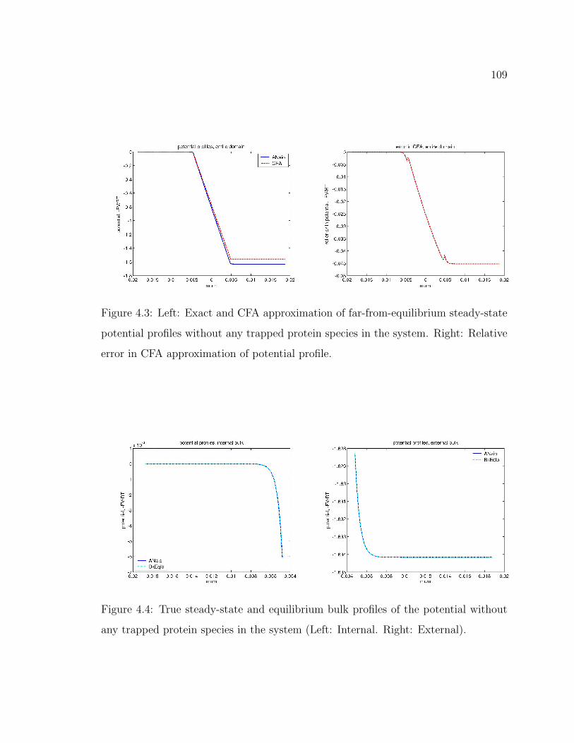
109
Figure 4.3: Left: Exact and CFA approximation of far-from-equilibrium steady-state
potential profiles without any trapped protein species in the system. Right: Relative
error in CFA approximation of potential profile.
Figure 4.4: True steady-state and equilibrium bulk profiles of the potential without
any trapped protein species in the system (Left: Internal. Right: External).

110
Figure 4.5: Relative error in equilibrium potential profiles at far-from-equilibrium
steady-state without any trapped protein species in the system. (Internal bulk (top),
membrane (mid), external bulk (bot)).
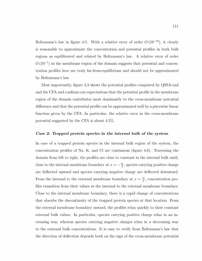
111
Boltzmann’s law in figure 4.5. With a relative error of order O (10−10), it clearly
is reasonable to approximate the concentration and potential profiles in both bulk
regions as equilibrated and related by Boltzmann’s law. A relative error of order
O (10−1) in the membrane region of the domain suggests that potential and concen-
tration profiles here are truly far-from-equilibrium and should not be approximated
by Boltzmann’s law.
Most importantly, figure 4.3 shows the potential profiles computed by QSSA-end
and the CFA and confirms our expectations that the potential profile in the membrane
region of the domain contributes most dominantly to the cross-membrane potential
difference and that the potential profile can be approximated well by a piecewise linear
function given by the CFA. In particular, the relative error in the cross-membrane
potential suggested by the CFA is about 4.5%.
Case 2: Trapped protein species in the internal bulk of the system
In case of a trapped protein species in the internal bulk region of the system, the
concentration profiles of Na, K, and Cl are continuous (figure 4.6). Traversing the
domain from left to right, the profiles are close to constant in the internal bulk until,
close to the internal membrane boundary at x = −m2, species carrying positive charge
are deflected upward and species carrying negative charge are deflected downward.
From the internal to the external membrane boundary at x = m2, concentration pro-
files transition from their values at the internal to the external membrane boundary.
Close to the internal membrane boundary, there is a rapid change of concentrations
that absorbs the discontinuity of the trapped protein species at that location. From
the external membrane boundary onward, the profiles relax quickly to their constant
external bulk values. In particular, species carrying positive charge relax in an in-
creasing way, whereas species carrying negative charges relax in a decreasing way
to the external bulk concentrations. It is easy to verify from Boltzmann’s law that
the direction of deflection depends both on the sign of the cross-membrane potential
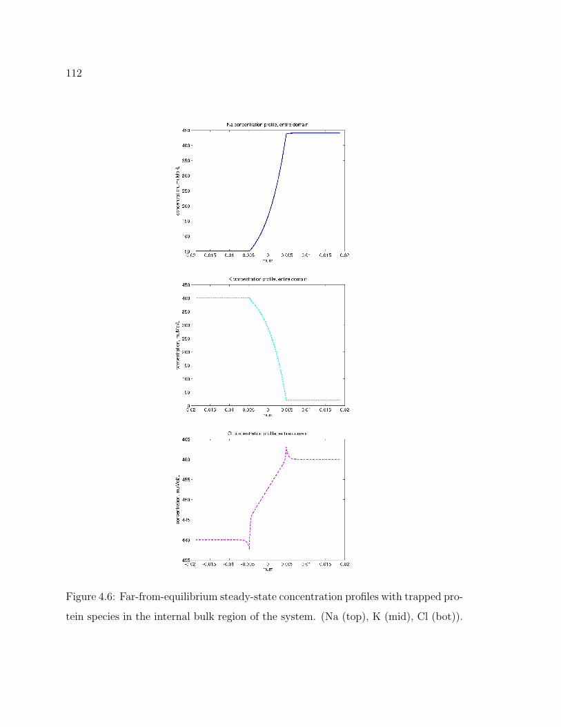
112
Figure 4.6: Far-from-equilibrium steady-state concentration profiles with trapped pro-
tein species in the internal bulk region of the system. (Na (top), K (mid), Cl (bot)).
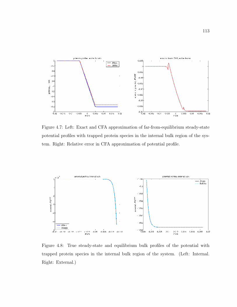
113
Figure 4.7: Left: Exact and CFA approximation of far-from-equilibrium steady-state
potential profiles with trapped protein species in the internal bulk region of the sys-
tem. Right: Relative error in CFA approximation of potential profile.
Figure 4.8: True steady-state and equilibrium bulk profiles of the potential with
trapped protein species in the internal bulk region of the system. (Left: Internal.
Right: External.)
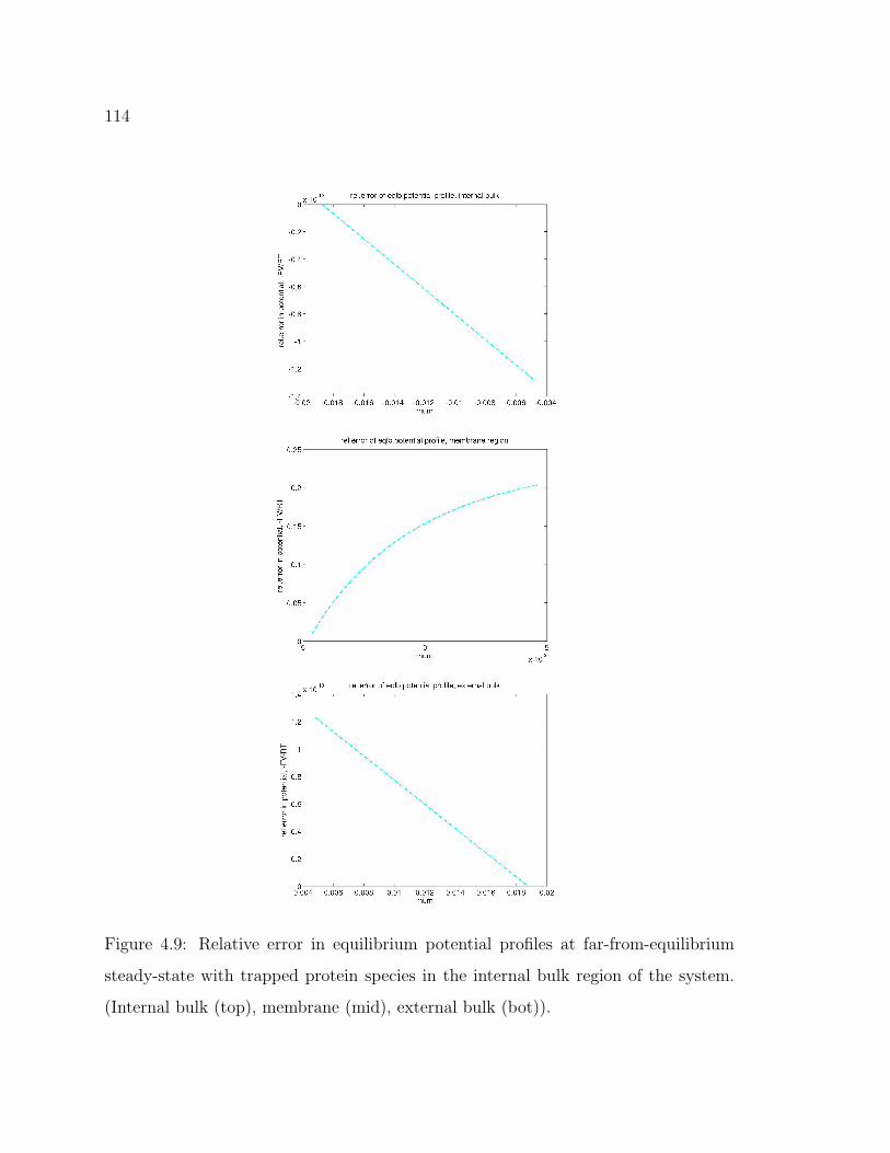
114
Figure 4.9: Relative error in equilibrium potential profiles at far-from-equilibrium
steady-state with trapped protein species in the internal bulk region of the system.
(Internal bulk (top), membrane (mid), external bulk (bot)).
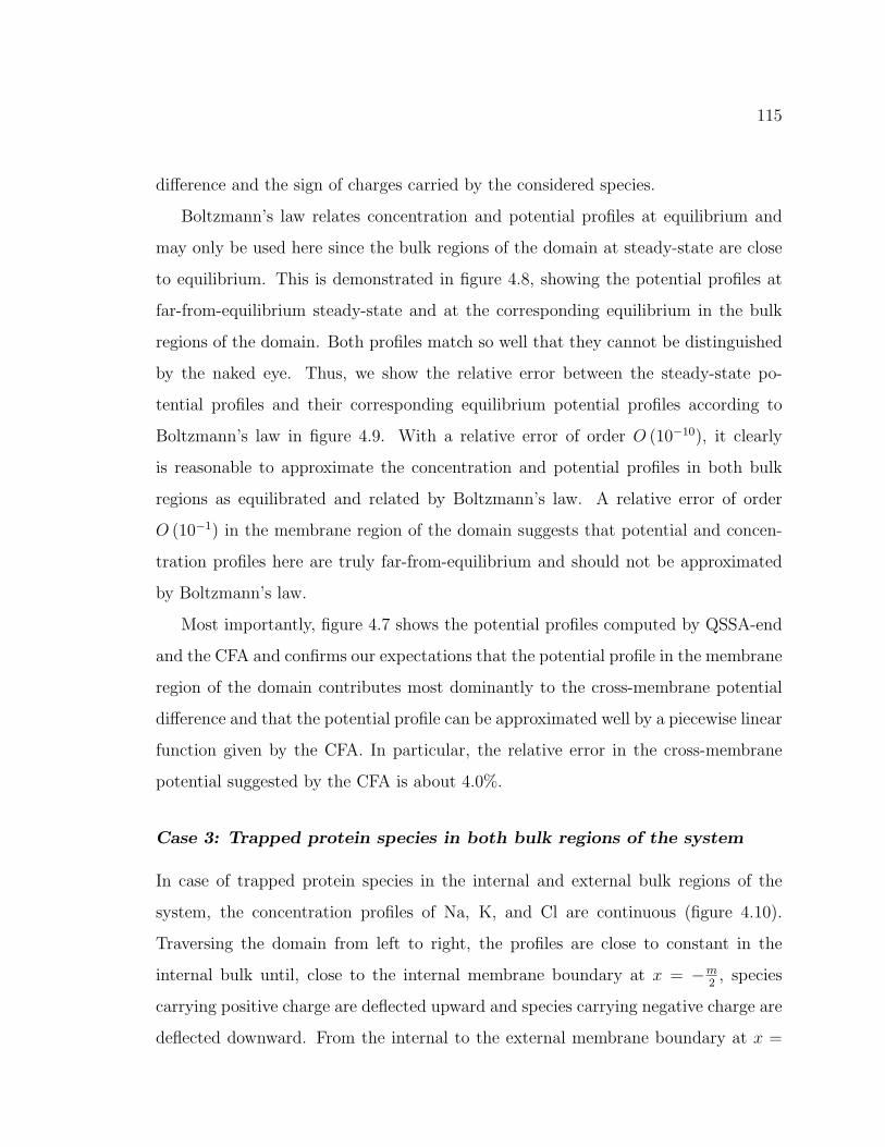
115
difference and the sign of charges carried by the considered species.
Boltzmann’s law relates concentration and potential profiles at equilibrium and
may only be used here since the bulk regions of the domain at steady-state are close
to equilibrium. This is demonstrated in figure 4.8, showing the potential profiles at
far-from-equilibrium steady-state and at the corresponding equilibrium in the bulk
regions of the domain. Both profiles match so well that they cannot be distinguished
by the naked eye. Thus, we show the relative error between the steady-state po-
tential profiles and their corresponding equilibrium potential profiles according to
Boltzmann’s law in figure 4.9. With a relative error of order O (10−10), it clearly
is reasonable to approximate the concentration and potential profiles in both bulk
regions as equilibrated and related by Boltzmann’s law. A relative error of order
O (10−1) in the membrane region of the domain suggests that potential and concen-
tration profiles here are truly far-from-equilibrium and should not be approximated
by Boltzmann’s law.
Most importantly, figure 4.7 shows the potential profiles computed by QSSA-end
and the CFA and confirms our expectations that the potential profile in the membrane
region of the domain contributes most dominantly to the cross-membrane potential
difference and that the potential profile can be approximated well by a piecewise linear
function given by the CFA. In particular, the relative error in the cross-membrane
potential suggested by the CFA is about 4.0%.
Case 3: Trapped protein species in both bulk regions of the system
In case of trapped protein species in the internal and external bulk regions of the
system, the concentration profiles of Na, K, and Cl are continuous (figure 4.10).
Traversing the domain from left to right, the profiles are close to constant in the
internal bulk until, close to the internal membrane boundary at x = −m2, species
carrying positive charge are deflected upward and species carrying negative charge are
deflected downward. From the internal to the external membrane boundary at x =
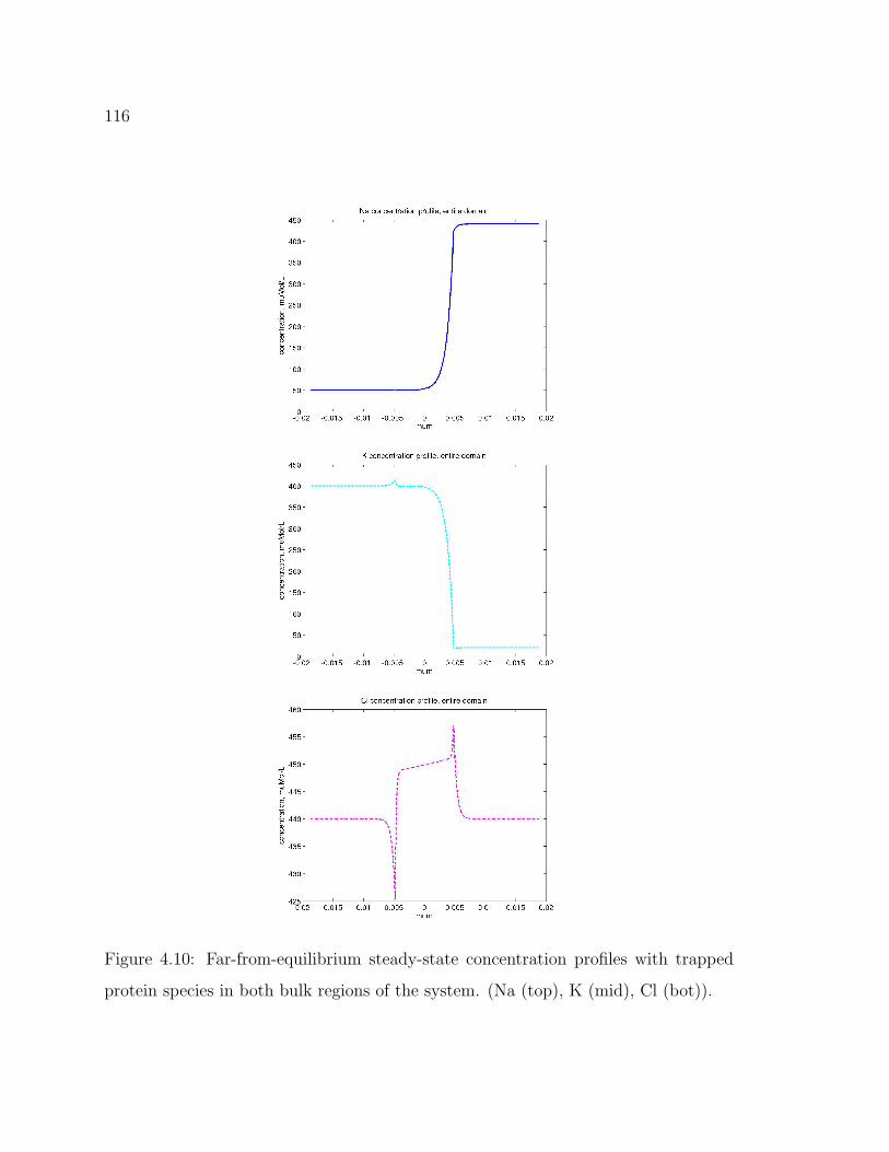
116
Figure 4.10: Far-from-equilibrium steady-state concentration profiles with trapped
protein species in both bulk regions of the system. (Na (top), K (mid), Cl (bot)).
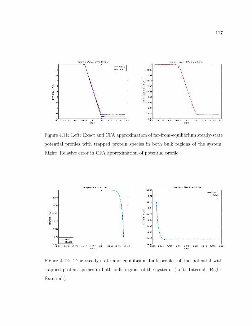
117
Figure 4.11: Left: Exact and CFA approximation of far-from-equilibrium steady-state
potential profiles with trapped protein species in both bulk regions of the system.
Right: Relative error in CFA approximation of potential profile.
Figure 4.12: True steady-state and equilibrium bulk profiles of the potential with
trapped protein species in both bulk regions of the system. (Left: Internal. Right:
External.)
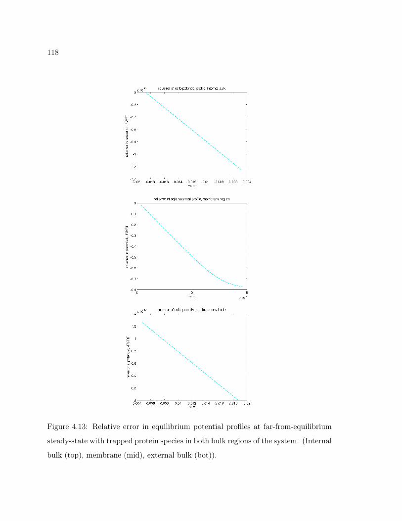
118
Figure 4.13: Relative error in equilibrium potential profiles at far-from-equilibrium
steady-state with trapped protein species in both bulk regions of the system. (Internal
bulk (top), membrane (mid), external bulk (bot)).

119
m2, concentration profiles transition from their values at the internal to the external
membrane boundary. Close to the internal and external membrane boundaries, there
is a rapid change of concentrations that absorbs the discontinuities of the trapped
protein species at those locations. From the external membrane boundary onward,
the profiles relax quickly to their constant external bulk values. In particular, species
carrying positive charge relax in an increasing way, whereas species carrying negative
charges relax in a decreasing way to the external bulk concentrations. It is easy to
verify from Boltzmann’s law that the direction of deflection depends both on the
sign of the cross-membrane potential difference and the sign of charges carried by the
considered species.
Boltzmann’s law relates concentration and potential profiles at equilibrium and
may only be used here since the bulk regions of the domain at steady-state are close
to equilibrium. This is demonstrated in figure 4.12, showing the potential profiles at
far-from-equilibrium steady-state and at the corresponding equilibrium in the bulk
regions of the domain. Both profiles match so well that they cannot be distinguished
by the naked eye. Thus, we show the relative error between the steady-state po-
tential profiles and their corresponding equilibrium potential profiles according to
Boltzmann’s law in figure 4.13. With a relative error of order O (10−10), it clearly
is reasonable to approximate the concentration and potential profiles in both bulk
regions as equilibrated and related by Boltzmann’s law. A relative error of order
O (10−1) in the membrane region of the domain suggests that potential and concen-
tration profiles here are truly far-from-equilibrium and should not be approximated
by Boltzmann’s law.
Most importantly, figure 4.11 shows the potential profiles computed by QSSA-end
and the CFA and confirms our expectations that the potential profile in the mem-
brane region of the domain contributes dominantly to the cross-membrane potential
difference and that the potential profile can be approximated well by a piecewise lin-
ear function given by the CFA. In particular, the relative error in the cross-membrane
120
potential suggested by the CFA is about 4.6%.
4.3 Linearization of the QSSA: the HH-plk Model
The second approximation of the QSSA is its linearization with respect to the electro-
static potential that results in a Hodgkin−Huxley-type model (HHplk). According
to the QSSA,
− Ji = Di
(dci
dx+ zi
dϕ
dxci
)= const. , (4.28)
with the diffusion coefficient of species i in membrane medium, Di. Thus, in partic-
ular,
− Ji = −Ji (0) = Di
(dci
dx(0) + zi
dϕ
dx(0) ci (0)
)(4.29)
= Dici (0)
(dci
dx(0)
ci (0)+ zi
dϕ
dx(0)
)(4.30)
= Dici (0)
(d (ln ci)
dx(0) + zi
dϕ
dx(0)
)(4.31)
≈ Dici (0)
m
(ln
ci (R)
ci (L)+ zi (ϕ (R)− ϕ (L))
). (4.32)
With previous notation and re-dimensionalizing, this flux density may be converted
into a current density, Ii, and may be written as
Ii = ziFJi ≈ −ziFDici (0)
m
(ln
ci (R)
ci (L)+ zi (ϕ (R)− ϕ (L))
)(4.33)
= −ziF δ2 Dici (0)
m
(ln
ci (R)
ci (L)− zi
FV
R0T
)(4.34)
=z2
i F2δ2Dici (0)
R0T m
(V − R0T
ziFln
ci (R)
ci (L)
)(4.35)
= gi
(V − V NP
i
). (4.36)
121
V NPi denotes the Nernst potential and gi denotes the conductance per unit area for
species i. Clearly,
V NPi =
R0T
ziFln
ci (R)
ci (L)(4.37)
≈ R0T
ziFln
couti
cini
and (4.38)
gi =z2
i F2δ2Dici (0)
R0T m. (4.39)
The cross-membrane potential difference, ∆ϕ, obeys the same equation as in the CFA,
(4.14), consistent with a Hodgkin−Huxley-type voltage equation with capacitance per
unit area of
Cm =F 2δ2c
R0T· εM
m=
ε0εr
m. (4.40)
The equations describing the dynamics of the HHplk model are, in summary,
vindcin
i
dt= −AcJi (4.41)
c>i = vincini + voutc
outi (4.42)
Ji =1
ziFIi =
1
ziFgi
(V − V NP
i
)(4.43)
V =m vinR0T
εMAcF
∑i
zicini (4.44)
V NPi =
R0T
ziFln
couti
cini
. (4.45)
Comparison of HHplk model to the classic HH model
What differentiates the HHplk model from the classic Hodgkin−Huxley (HH) model
is that in the HHplk model, the cross-membrane potential difference is determined
directly from the average internal concentrations, cini , according to an approximation
of Poisson’s equation, whereas HH uses an ODE for the cross-membrane voltage based
122
upon the current-voltage relationship in a model circuit that includes a capacitor and
multiple conductances (see also figure 1.10). Thus, the HHplk model requires its
bulk concentrations to be net electro-neutral and its average internal and external
concentrations to be close to net electro-neutral, whereas the HH model does not
require or consider electro-neutrality. Furthermore, HHplk models a closed, finite-
volume, two-compartment system in which concentrations obey conditions of mass
conservation, whereas HH describes an open system, in which the concentrations
are infinitely well-buffered. The, so far passive, currents in HHplk depend on the
Nernst potential which in turn depends on the dynamically evolving average bulk
concentrations, whereas HH does not distinguish between active and passive currents.
Instead, both are empirically captured by the so-called reversal potential, a system
parameter specific to each ion species. The issue of active and passive transport across
the membrane shall be discussed in more detail in section 4.4, where active transport
is added to the, so far passive, CFA and HHplk models.
4.4 Dynamic approach to the equilibrium of a cell
After deriving two different approximations of the QSSA-end in sections 4.2 and 4.3
and confirming in subsection 4.2.2 that the CFA approximates the QSSA-end well
at various far-from-equilibrium steady-states, we now compare the dynamics by the
QSSA-end, CFA, and HHplk models. For this purpose, we consider a cell with HH-
type, gated ion channels but no ion pumps that actively transport ions against their
electro-chemical gradient and thereby maintain homeostasis. It is understood that the
diffusion coefficients in the QSSA-end and CFA based models and the conductances in
the HHplk based model include gating terms and that the dynamic equations defining
each model are enhanced by the classic HH gating dynamics, (see subsection 1.3.1).
The system containing Na, K, and Cl is initialized at a far-from-equilibrium steady-
state close to the natural resting state of the cell. Since active transport is lacking,
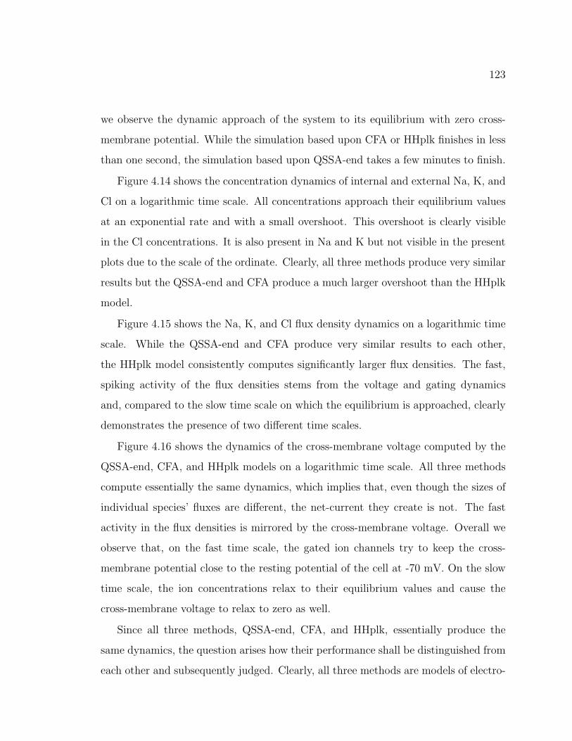
123
we observe the dynamic approach of the system to its equilibrium with zero cross-
membrane potential. While the simulation based upon CFA or HHplk finishes in less
than one second, the simulation based upon QSSA-end takes a few minutes to finish.
Figure 4.14 shows the concentration dynamics of internal and external Na, K, and
Cl on a logarithmic time scale. All concentrations approach their equilibrium values
at an exponential rate and with a small overshoot. This overshoot is clearly visible
in the Cl concentrations. It is also present in Na and K but not visible in the present
plots due to the scale of the ordinate. Clearly, all three methods produce very similar
results but the QSSA-end and CFA produce a much larger overshoot than the HHplk
model.
Figure 4.15 shows the Na, K, and Cl flux density dynamics on a logarithmic time
scale. While the QSSA-end and CFA produce very similar results to each other,
the HHplk model consistently computes significantly larger flux densities. The fast,
spiking activity of the flux densities stems from the voltage and gating dynamics
and, compared to the slow time scale on which the equilibrium is approached, clearly
demonstrates the presence of two different time scales.
Figure 4.16 shows the dynamics of the cross-membrane voltage computed by the
QSSA-end, CFA, and HHplk models on a logarithmic time scale. All three methods
compute essentially the same dynamics, which implies that, even though the sizes of
individual species’ fluxes are different, the net-current they create is not. The fast
activity in the flux densities is mirrored by the cross-membrane voltage. Overall we
observe that, on the fast time scale, the gated ion channels try to keep the cross-
membrane potential close to the resting potential of the cell at -70 mV. On the slow
time scale, the ion concentrations relax to their equilibrium values and cause the
cross-membrane voltage to relax to zero as well.
Since all three methods, QSSA-end, CFA, and HHplk, essentially produce the
same dynamics, the question arises how their performance shall be distinguished from
each other and subsequently judged. Clearly, all three methods are models of electro-
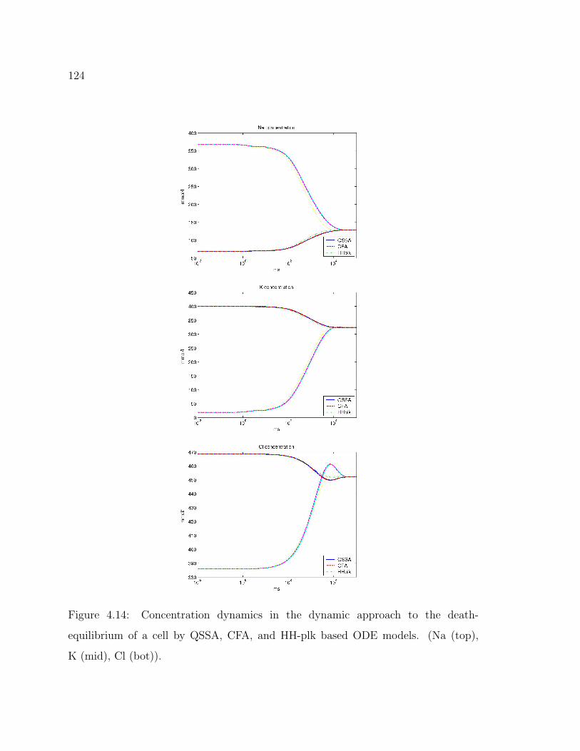
124
Figure 4.14: Concentration dynamics in the dynamic approach to the death-
equilibrium of a cell by QSSA, CFA, and HH-plk based ODE models. (Na (top),
K (mid), Cl (bot)).
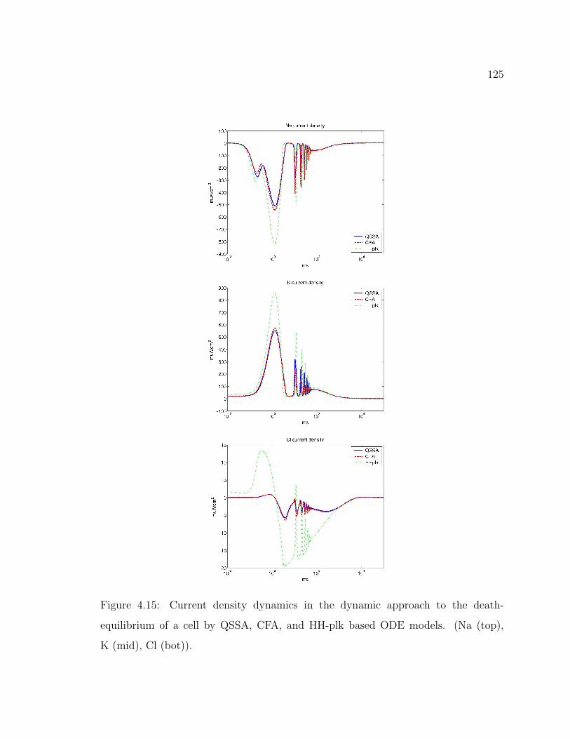
125
Figure 4.15: Current density dynamics in the dynamic approach to the death-
equilibrium of a cell by QSSA, CFA, and HH-plk based ODE models. (Na (top),
K (mid), Cl (bot)).
126
Figure 4.16: Cross-membrane potential dynamics in the dynamic approach to the
death equilibrium of a cell by QSSA, CFA, and HH-plk based ODE models.
diffusion and thus, a measure is desired that indicates how well the intricate processes
underlying electro-diffusion are approximated by each method. The maintenance of
electro-neutrality in each of the compartments has been an issue throughout this
work. In this spirit, note that according to the electro-diffusion equation,
− zidϕ
dxci =
dci
dx+
Ji
Di
(4.46)
and reconsider Poisson’s equation,
d
dx
(εdϕ
dx
)= −
∑i
zici (4.47)(εdϕ
dx
)d
dx
(εdϕ
dx
)= −ε
∑i
zidϕ
dxci (4.48)
d
dx
1
2
(εdϕ
dx
)2 = ε
∑i
dci
dx+
Ji
Di
(4.49)
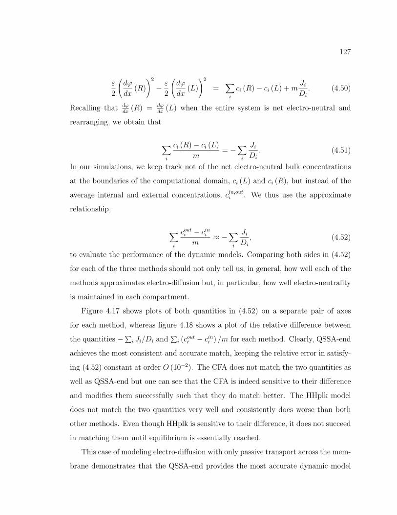
127
ε
2
(dϕ
dx(R)
)2
− ε
2
(dϕ
dx(L)
)2
=∑
i
ci (R)− ci (L) + mJi
Di
. (4.50)
Recalling that dϕdx
(R) = dϕdx
(L) when the entire system is net electro-neutral and
rearranging, we obtain that
∑i
ci (R)− ci (L)
m= −
∑i
Ji
Di
. (4.51)
In our simulations, we keep track not of the net electro-neutral bulk concentrations
at the boundaries of the computational domain, ci (L) and ci (R), but instead of the
average internal and external concentrations, cin,outi . We thus use the approximate
relationship,
∑i
couti − cin
i
m≈ −
∑i
Ji
Di
, (4.52)
to evaluate the performance of the dynamic models. Comparing both sides in (4.52)
for each of the three methods should not only tell us, in general, how well each of the
methods approximates electro-diffusion but, in particular, how well electro-neutrality
is maintained in each compartment.
Figure 4.17 shows plots of both quantities in (4.52) on a separate pair of axes
for each method, whereas figure 4.18 shows a plot of the relative difference between
the quantities −∑i Ji/Di and∑
i (couti − cin
i ) /m for each method. Clearly, QSSA-end
achieves the most consistent and accurate match, keeping the relative error in satisfy-
ing (4.52) constant at order O (10−2). The CFA does not match the two quantities as
well as QSSA-end but one can see that the CFA is indeed sensitive to their difference
and modifies them successfully such that they do match better. The HHplk model
does not match the two quantities very well and consistently does worse than both
other methods. Even though HHplk is sensitive to their difference, it does not succeed
in matching them until equilibrium is essentially reached.
This case of modeling electro-diffusion with only passive transport across the mem-
brane demonstrates that the QSSA-end provides the most accurate dynamic model
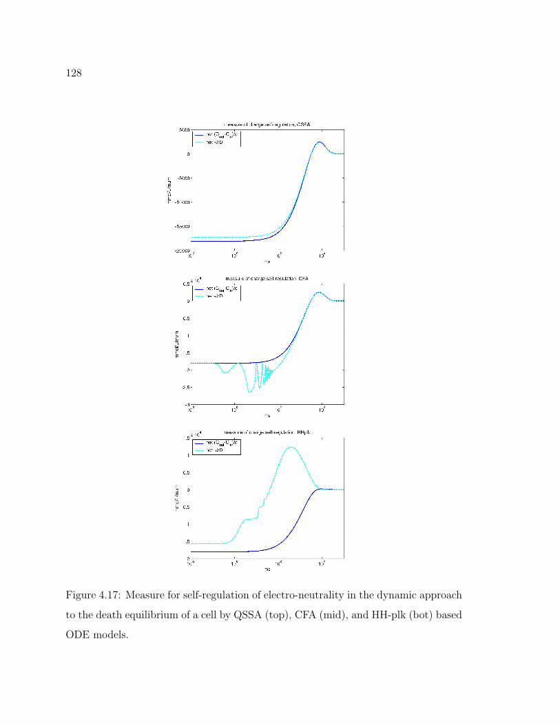
128
Figure 4.17: Measure for self-regulation of electro-neutrality in the dynamic approach
to the death equilibrium of a cell by QSSA (top), CFA (mid), and HH-plk (bot) based
ODE models.
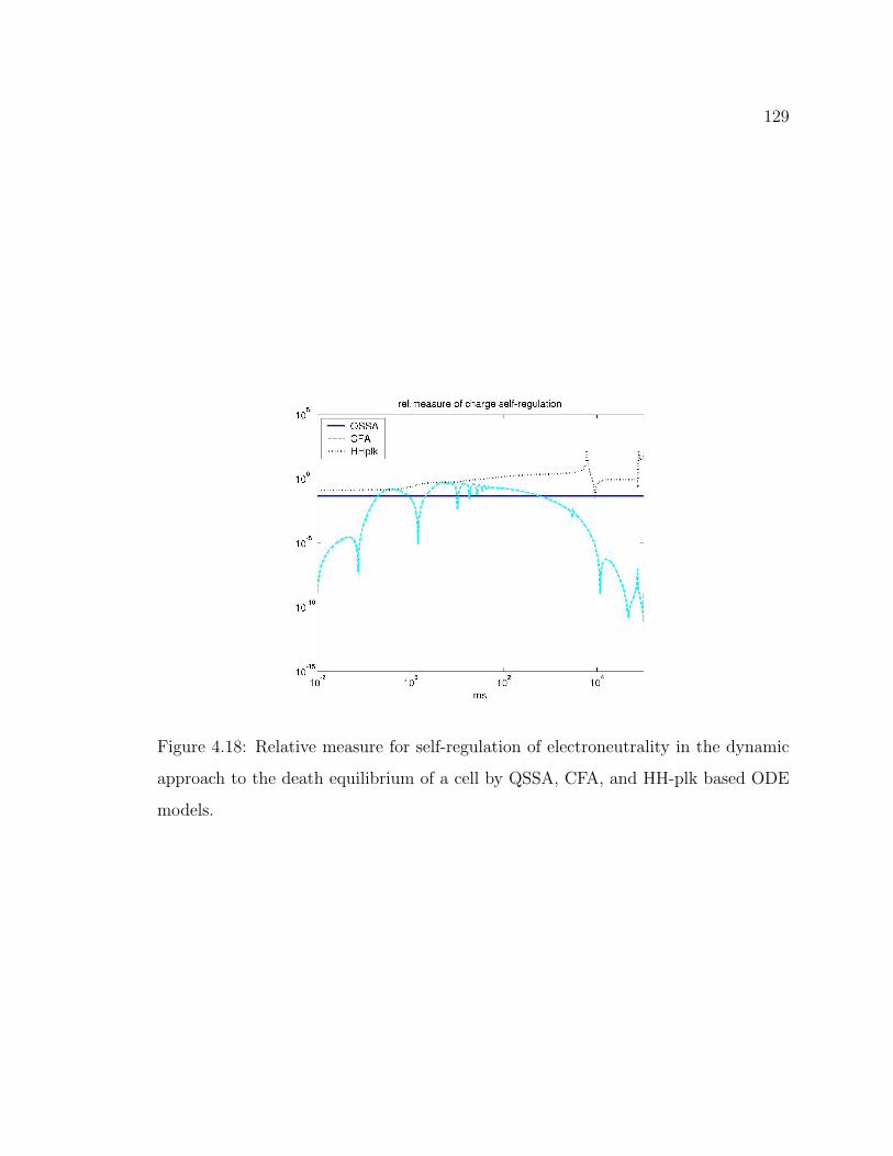
129
Figure 4.18: Relative measure for self-regulation of electroneutrality in the dynamic
approach to the death equilibrium of a cell by QSSA, CFA, and HH-plk based ODE
models.
130
of electro-diffusion. It also demonstrates that the CFA provides a reasonably accu-
rate model of electro-diffusion by actively maintaining electro-neutrality in the bulk.
In addition, as a pure ODE model, CFA is easily adjusted to incorporate active ion
transport against electro-chemical gradients. Even though QSSA-end takes a few
minutes to run, it is worth using when its improved accuracy is desired. However, it
does require a steady-state problem to be solved at each time step and is not easily
adjusted to include active ion transport against electro-chemical gradients. QSSA-end
is, in this sense, restricted to the case of electro-diffusion with only passive transport
across the membrane.
4.5 Sustaining the living state of a cell
In the following, CFA and HHplk shall be updated to incorporate active ion transport
against electro-chemical gradients. This will enable both models to maintain home-
ostasis and thus, to be compared to the classic Hodgkin−Huxley model. Including
active transport in QSSA-end means to include sources and sinks in the computa-
tional domain, that is an entirely different steady-state problem needs to be solved.
Furthermore, if source contributions represent point-sources or -sinks, the adjusted
problem is expected to be stiff so that the steady-state solver may converge slowly. In
this case, the steady-state solver in the adjusted QSSA-end would not be efficient as
part of a dynamic simulation. Incorporating sources and sinks in the computational
domain as result of active ion transport shall thus not be considered here but instead
be left as a future challenge. See section B.2 for the equations defining an adjusted
steady-state solver that incorporates source contributions from space-dependent but
concentration-independent sources.
In subsection 4.5.1, a simple model of ion pump fluxes responsible for maintaining
certain concentration gradients associated with homeostasis is introduced. In subsec-
tion 4.5.2, it is demonstrated that CFA and HHplk are able to maintain a steady-state
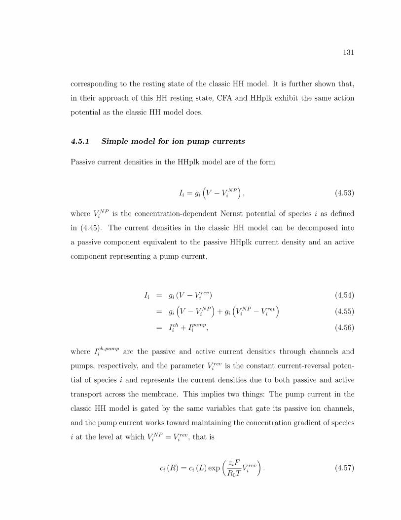
131
corresponding to the resting state of the classic HH model. It is further shown that,
in their approach of this HH resting state, CFA and HHplk exhibit the same action
potential as the classic HH model does.
4.5.1 Simple model for ion pump currents
Passive current densities in the HHplk model are of the form
Ii = gi
(V − V NP
i
), (4.53)
where V NPi is the concentration-dependent Nernst potential of species i as defined
in (4.45). The current densities in the classic HH model can be decomposed into
a passive component equivalent to the passive HHplk current density and an active
component representing a pump current,
Ii = gi (V − V revi ) (4.54)
= gi
(V − V NP
i
)+ gi
(V NP
i − V revi
)(4.55)
= Ichi + Ipump
i , (4.56)
where Ich,pumpi are the passive and active current densities through channels and
pumps, respectively, and the parameter V revi is the constant current-reversal poten-
tial of species i and represents the current densities due to both passive and active
transport across the membrane. This implies two things: The pump current in the
classic HH model is gated by the same variables that gate its passive ion channels,
and the pump current works toward maintaining the concentration gradient of species
i at the level at which V NPi = V rev
i , that is
ci (R) = ci (L) exp(
ziF
R0TV rev
i
). (4.57)
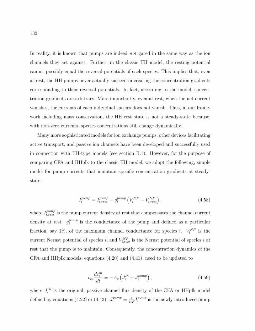
132
In reality, it is known that pumps are indeed not gated in the same way as the ion
channels they act against. Further, in the classic HH model, the resting potential
cannot possibly equal the reversal potentials of each species. This implies that, even
at rest, the HH pumps never actually succeed in creating the concentration gradients
corresponding to their reversal potentials. In fact, according to the model, concen-
tration gradients are arbitrary. More importantly, even at rest, when the net current
vanishes, the currents of each individual species does not vanish. Thus, in our frame-
work including mass conservation, the HH rest state is not a steady-state because,
with non-zero currents, species concentrations still change dynamically.
Many more sophisticated models for ion exchange pumps, other devices facilitating
active transport, and passive ion channels have been developed and successfully used
in connection with HH-type models (see section B.1). However, for the purpose of
comparing CFA and HHplk to the classic HH model, we adopt the following, simple
model for pump currents that maintain specific concentration gradients at steady-
state:
Ipumpi = Ipump
i,rest − gpumpi
(V NP
i − V NPi,rest
), (4.58)
where Ipumpi,rest is the pump current density at rest that compensates the channel current
density at rest. gpumpi is the conductance of the pump and defined as a particular
fraction, say 1%, of the maximum channel conductance for species i. V NPi is the
current Nernst potential of species i, and V NPi,rest is the Nernst potential of species i at
rest that the pump is to maintain. Consequently, the concentration dynamics of the
CFA and HHplk models, equations (4.20) and (4.41), need to be updated to
vindcin
i
dt= −Ac
(J ch
i + Jpumpi
), (4.59)
where J chi is the original, passive channel flux density of the CFA or HHplk model
defined by equations (4.22) or (4.43). Jpumpi = 1
ziFIpumpi is the newly introduced pump
133
Figure 4.19: Resting state of HH at -70 mV is maintained by CFA and HHplk (left).
Net currents do not vanish for HH and thus, for example, Na concentrations are
maintained by CFA and HHplk but blow up over time for HH (right).
flux density for species i and is defined through (4.58).
4.5.2 Numerical simulations and results
To be able to compare the CFA and HHplk models to the classic HH model, it is un-
derstood that the diffusion and dielectric coefficients have to match the conductances
and capacitance according to (4.39) and (4.40) and that the gating variables from the
classic HH model along with their dynamics are used in all three models. We further
set the steady-state concentrations of Na, K, and Cl at physiologically reasonable
levels that result in a cross-membrane potential of -70 mV, the resting potential of
the classic HH model. We then define the resulting Nernst potentials, channel fluxes,
and pump fluxes for each species at rest. This defines all parameters needed to run
all models and ensures that the CFA, HHplk, and classic HH models share not only
dynamic parameters but also a corresponding steady-state.
To demonstrate that all three models maintain the same resting state, we initialize
all models at rest. Figure 4.19 shows the constant resting potential maintained at
134
Figure 4.20: Relative measure for self-regulation of bulk electro-neutrality by the
CFA, HHplk, and classic HH models at rest. The downward spike in the HH model
is produced by a crossing of the two quantities whose relative difference is shown.
-70 mV. The lines created by CFA, HHplk and HH cannot be distinguished from
each other by the naked eye. Computing the relative error of all methods, not shown
here, demonstrates that HH and HHplk match -70 mV to machine precision and that
the relative error in CFA is of order O (10−11). Figure 4.19 also shows that CFA
and HHplk maintain the Na ion concentrations at their steady-state levels, whereas
Na concentrations blow up for HH as a result of its non-vanishing Na net currents.
Dynamics of K and Cl are qualitatively the same.
Figure 4.20 shows the relative difference between the quantities −∑i Ji/Di and∑i (c
outi − cin
i ) /m, a performance measure defined by equation (4.52) that indicates
how well electro-neutrality is maintained in the bulk compartments. Recall that equa-
tion (4.52) describes an approximate relationship that best fits its exact counterpart
at small cross-membrane potentials, that is when little net charge is accumulated at
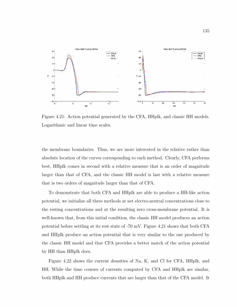
135
Figure 4.21: Action potential generated by the CFA, HHplk, and classic HH models.
Logarithmic and linear time scales.
the membrane boundaries. Thus, we are more interested in the relative rather than
absolute location of the curves corresponding to each method. Clearly, CFA performs
best, HHplk comes in second with a relative measure that is an order of magnitude
larger than that of CFA, and the classic HH model is last with a relative measure
that is two orders of magnitude larger than that of CFA.
To demonstrate that both CFA and HHplk are able to produce a HH-like action
potential, we initialize all three methods at net electro-neutral concentrations close to
the resting concentrations and at the resulting zero cross-membrane potential. It is
well-known that, from this initial condition, the classic HH model produces an action
potential before settling at its rest state of -70 mV. Figure 4.21 shows that both CFA
and HHplk produce an action potential that is very similar to the one produced by
the classic HH model and that CFA provides a better match of the action potential
by HH than HHplk does.
Figure 4.22 shows the current densities of Na, K, and Cl for CFA, HHplk, and
HH. While the time courses of currents computed by CFA and HHplk are similar,
both HHplk and HH produce currents that are larger than that of the CFA model. It

136
Figure 4.22: Current densities of Na (top), K (mid), and Cl (bot) that shape the
action potential produced by the CFA, HHplk, and classic HH models.
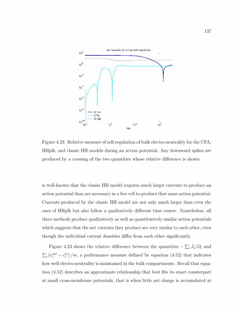
137
Figure 4.23: Relative measure of self-regulation of bulk electro-neutrality for the CFA,
HHplk, and classic HH models during an action potential. Any downward spikes are
produced by a crossing of the two quantities whose relative difference is shown.
is well-known that the classic HH model requires much larger currents to produce an
action potential than are necessary in a live cell to produce that same action potential.
Currents produced by the classic HH model are not only much larger than even the
ones of HHplk but also follow a qualitatively different time course. Nonetheless, all
three methods produce qualitatively as well as quantitatively similar action potentials
which suggests that the net currents they produce are very similar to each other, even
though the individual current densities differ from each other significantly.
Figure 4.23 shows the relative difference between the quantities −∑i Ji/Di and∑i (c
outi − cin
i ) /m, a performance measure defined by equation (4.52) that indicates
how well electro-neutrality is maintained in the bulk compartments. Recall that equa-
tion (4.52) describes an approximate relationship that best fits its exact counterpart
at small cross-membrane potentials, that is when little net charge is accumulated at
138
the membrane boundaries. Thus, we are more interested in the relative rather than
absolute location of the curves corresponding to each method. Clearly, CFA performs
best, HHplk comes in second with a relative measure that is about an order of magni-
tude larger than that of CFA, and the classic HH model is last with a relative measure
that is closer to two orders of magnitude larger than that of CFA.
4.6 Summary of Results
We have adjusted the quasi steady-state approximation (QSSA) of electro-diffusion
from the setting of mid-membrane impermeability to the more realistic setting of
end-of-membrane impermeability. In this setting, species impermeable to the mem-
brane cannot enter the membrane at all and the computational domain has to include
parts of the internal and external bulk regions, in which small amounts of net charge
accumulate. The full electro-diffusion system is not efficiently solved due to the fast
dynamics in the bulk which has thus not been attempted here. Instead, we trust that
the QSSA for end-of-membrane impermeability (QSSA-end) approximates individual
steady-states and the dynamics of the full electro-diffusion system well. Then, two
different approximations of the QSSA-end are derived.
The first approximation of QSSA-end, based on a constant field approximation
(CFA), yields a piecewise linear approximation of the electro-static potential and
GHK-like flux densities. The CFA is demonstrated to match the potential profile of
the QSSA-end reasonably well. Further, its cross-membrane potential is consistent
with a HH-like voltage equation, even though it is not derived from an electric model
circuit but instead determined directly from the net charge accumulated around one
of the membrane boundaries. The most important difference between the CFA and
the classic HH-GHK model is that CFA is formally derived from electro-diffusion,
obeys mass conservation, and determines the cross-membrane potential directly from
the average internal or external concentrations, whereas HH-GHK models an open
139
system with no mass conservation that determines its cross-membrane potential from
the current-voltage relationship in an electric model circuit. As a result, CFA is
sensitive to charges accumulating in either compartment. It actively self-regulates
bulk electro-neutrality, whereas HH-GHK does not. The second approximation of
QSSA-end, based on a linearization of QSSA-end, yields the HHplk model, which is
equivalent to a combination of classic HH and pump-leak models that are additionally
subject to mass conservation conditions.
The CFA and HHplk models derived from electro-diffusion incorporate no active
transport at this point that would allow them to maintain their concentration gra-
dients at levels associated with homeostasis. Thus, the dynamics of the CFA and
HHplk models are compared to the dynamics of QSSA-end for the approach to equi-
librium of a cell with gated ion channels but no active transport that would allow it
to maintain homeostasis. All models produce similar results for the cross-membrane
potential, ion fluxes, and concentration dynamics. In order to distinguish the quality
of those results more clearly, we have developed a measure that indicates not only how
well electro-diffusion is modeled but, in particular, how well each method maintains
electro-neutrality in the bulk of the compartments. Based on this measure, QSSA-end
provides the most accurate dynamic model of electro-diffusion but requires a steady-
state problem to be solved at each time step. CFA provides a reasonably accurate
and highly efficient model of electro-diffusion. While bulk electro-neutrality is not
maintained as well as by QSSA-end, CFA is clearly sensitive to charges accumulating
in the bulk, successfully adjusts them to achieve a better result, and is described only
by a system of ODEs. HHplk is also described only by a system of ODEs and effi-
ciently solved but is much less sensitive to charges accumulating in bulk. In summary,
QSSA-end provides the most accurate model, whereas CFA provides a very efficient
and reasonably accurate model of passive electro-diffusion.
In moving toward modeling a live cell with passive and active transport that
maintains homeostasis naturally, active transport in the form of pump fluxes was
140
incorporated into CFA and HHplk. Incorporating active transport in the QSSA-end
would mean solving an entirely different steady-state problem at each time step and
was not attempted here. Instead, classic HH fluxes were decomposed into their active
and passive components, and a related but more simple and consistent model of pump
fluxes was adopted and incorporated into the CFA and HHplk models. The dynamics
of the CFA, HHplk, and classic HH models were compared to each other for the
dynamic approach to rest from a nearby state with zero cross-membrane potential. All
three models have exhibited almost the same action potential before settling at their
common resting state. This suggests that the net current produced by all methods is
almost the same, even though the individual species’ fluxes are quite different from
each other. The classic HH model produces much larger fluxes that also follow a
qualitatively different time course than the ones of either CFA or HHplk. While the
fluxes produced by HHplk follow qualitatively the same time course as the ones by
CFA do, the fluxes by HHplk are larger. Comparing the three methods based on the
measure of self-regulation of bulk electro-neutrality, CFA clearly emerges as the most
accurate model. The efficiencies of CFA, HHplk, and classic HH are comparable. In
summary, CFA provides the most accurate model of both cross-membrane potential
and ion transport between a living cell and its finite environment.
141
Chapter 5
CONCLUSIONS AND FUTURE WORK
In chapter 1, I have given an introduction to the anatomy and function of the
brain and to various models of neurons and membrane transport, including the classic
Hodgkin−Huxley (HH) ODE model for neuron signal generation. I have discussed
the applicability of available models to in tissue modeling of cells, in which a cell is
interacting with its relatively small, finite environment instead of being bathed in an
infinitely well-buffered medium. The latter is assumed in most HH-type models and
causes problems when, as is critical in a finite environment, bulk electro-neutrality
needs to be maintained. Thus, the need for a physio-chemically consistent model for
ion transport and electric signal generation was established.
In chapter 2, I have studied electro-diffusion as a fundamental and physio-chemically
consistent model of the electro-static potential during passive ion transport across a
thin, lipid membrane. Under the assumptions of uniformity, homogeneity, and that
the compartments on either side of the membrane are large compared to the space
occupied by membrane medium, the problem was reduced to 1D. In the following,
I discussed the issues involved in solving the fully transient electro-diffusion system,
a system of nonlinearly coupled PDEs, numerically. Then, a quasi steady-state ap-
proximation (QSSA) of electro-diffusion was derived as a model for the dynamics of
electro-diffusion and based on the existence of two separate time-scales. Further, an
estimate for the time constant of the exponential approach of an electro-diffusion sys-
tem to its equilibrium was derived and shown to provide an accurate, a priori predic-
tion of the dynamic approach to equilibrium. Finally, analytic equilibrium solutions
of the electro-diffusion system were computed for various constellations of valencies
142
in the system. In summary, I have presented all analytic work that is relevant to my
goals and directly related to the highly nonlinear electro-diffusion system.
In chapter 3, numeric solution schemes for the fully transient electro-diffusion
system and its QSSA were discussed and developed. I have verified the existence
of a fast and slow time-scale by demonstrating numerically that the fully transient
electro-diffusion system enters consecutive steady-state dynamics on a very fast time-
scale. Thus, the QSSA provides an accurate model of electro-diffusion on the slower
time-scale on which the two compartments interact through the membrane.
In chapter 4, two different approximations of the QSSA were derived. These
approximations were motivated by the fact that, when simulating dynamics based on
the QSSA, a steady-state problem has to be solved at each time step and that thus,
a more efficient model consisting of just ODEs is desirable. The first approximation
of the QSSA was based on a constant field approximation (CFA) of the electro-
static potential, whereas the second approximation results from a linearization of the
QSSA and yields a combination of a HH-type with a pump-leak model (HHplk). In
contrast to previous models that incorporate these same assumptions, CFA and HHplk
determine the cross-membrane potential directly from the net-charge accumulated
near the membrane boundaries in either compartment instead of an electric model
circuit. Further, CFA and HHplk are subject to mass conservation conditions.
The dynamics of CFA and HHplk were compared to the dynamics of the QSSA
in the absence of active transport against electro-chemical gradients. Since all three
methods produced qualitatively and quantitatively similar results, I have developed
a measure that indicates not only how well electro-diffusion is modeled but, in par-
ticular, how well bulk electro-neutrality is maintained by each method. According to
this measure, the QSSA provides the most accurate model and CFA provides a more
efficient and reasonably accurate model of passive electro-diffusion, whereas HHplk is
not very successful in self-regulating bulk electro-neutrality. Thus, CFA is a candidate
for replacing QSSA with an accurate, more efficiently solved, and thus more desirable
143
model of electro-diffusion.
In moving toward modeling a live cell with passive and active transport that
maintains homeostasis naturally, I have incorporate active transport in the form of
pump fluxes into CFA and HHplk. Incorporating active transport in the QSSA would
mean solving an entirely different steady-state problem at each time step and was
not attempted here. Instead, classic HH fluxes were decomposed into their active and
passive components, and a related but more simple and consistent model of pump
fluxes was adopted and incorporated into the CFA and HHplk models. The dynamics
of the CFA, HHplk, and classic HH models were compared to each other for the
dynamic approach to rest from a nearby state with zero cross-membrane potential.
All three models produced essentially the same action potential. Based upon the
measure for self-regulation of bulk electro-neutrality, CFA clearly emerged as the
most accurate model for cross-membrane potential and ion transport in terms of its
physio-chemical consistency.
In summary, CFA provides an efficient means to accurately model the interactions
between two compartments with finite volume across a thin, lipid membrane. It is
thus uniquely qualified to model the ion transport and potential difference across
membranes of cells that interact with a relatively small external environment, as is
the case for cells in tissue.
5.1 Future Work
In future work, one might address the following:
1. Conduct a full analysis of the CFA model including the location and stability
of steady-states as well as bursting dynamics in various parameter regimes.
2. Include more sophisticated ion channels for Na and K, add Ca ions and their
buffering, and use more accurate descriptions of active pump fluxes in the CFA
144
(see section B.1).
3. Incorporate energetics into the CFA cell model by, for example, including ATP-
sensitive, and ATP-consuming, pumps and transporters.
4. Modify the CFA to accommodate volume dynamics (see appendix A) and study
whether and how the qualitative behavior of its solutions changes.
5. Incorporate active ion transport in the QSSA by including space-dependent but
concentration-independent source distributions in the electro-diffusion equation
(see section B.2).
6. Characterize the transient, pseudo steady-state in the approach to Donnan equi-
librium, which establishes on the order of ms and persists for some tens of ms
(compare section 3.3). We expect to utilize an energetic framework.
7. Study two neighboring cells with volume dynamics that share an external envi-
ronment with the goal to distinguish between cell-cell interactions through gap
junctions versus other ephaptic means.
8. Move toward tissue modeling by deriving equations that model networks of CFA
cells and thus represent pieces of tissue.
145
GLOSSARY
ACTION POTENTIAL: Relatively large transient detour of the cross-membrane po-
tential difference from its resting state. Threshold phenomenon fundamental to
synaptic signaling.
AXON: Signaling cable of the neuron cell. Long, little branched outgrowth from
the soma ending in axon terminals at chemical synapses.
BACK-UP: Copy of a file to be used when catastrophe strikes the original. People
who make no back-ups deserve no sympathy.
CENTRAL NERVOUS SYSTEM: Brain and spinal cord.
CORTEX: Also, cerebral cortex. The layer of gray matter covering most of the
surface of the brain.
CYTOSOLIC: Located in or having to do with the main internal compartment of
a cell.
DENDRITES: Signal detecting “antennae” of the neuron cell. Strongly branched
outgrowth leading stimuli toward the soma.
DONNAN EQUILIBRIUM: Equilibrium of a two-compartment system containing charged
particles, in which some particles are confined to one of the compartments. First
explored in detail by Donnan.
EPILEPSY: Any one of about 20 symptomatically classified forms of a complex
neural disease, collectively referred to as epilepsy.
146
EQUILIBRIUM: Steady-state with zero flux, or so-called “detailed balance”. Char-
acteristic of a closed system.
GAP JUNCTION: Trans-membrane protein that conjoins two neighboring neurons
and enables direct interaction between these cells’ cytosols.
GHK: Abbreviation: Goldman, Hodgkin and Katz.
INTERSTITIAL: Located in or having to do with the space by which cells in tissue
are separated from each other.
NEURON: Highly specialized cell of the nervous system that actively utilizes vari-
ations in its cross-membrane potential difference for signaling purposes.
HH: Abbreviation: Hodgkin and Huxley.
LOBE: Anatomically defined component of the brain, e.g., temporal lobe.
QSSA: Abbreviation: Quasi steady-state approximation.
SOMA: Main body of a neuron cell containing the cell nucleus and cell organelles.
STEADY-STATE: State at which the rate of change of system variables vanishes.
Steady-states with non-zero flux can only be maintained while expending energy,
and hence are characteristic of open systems.
SYNAPSE: Space between axon terminals and their downstream signaling targets.
TEMPORAL LOBE: The lobe of the brain located near the temples. Its main func-
tion is the formation and retaining of memory.
147
BIBLIOGRAPHY
[1] Amit, D.J. Modeling Brain Function. Cambridge University Press, New York.
(1989)
[2] Amster P. and Pinnau R. Convergent iterative schemes for a non-isentropic hy-
drodynamic model for semiconductors. Z. Angew. Math. Mech. 82: 559−566.
(2002)
[3] Babloyantz A. and Destexhe A. Low dimensional chaos in an instance of epilepsy.
Proc. Natl. Acad. Sci. USA 83: 3513−3517. (1986)
[4] Bach K.H., Dirks H.K., Meinerzhagen B., et al. A new nonlinear relaxation
scheme for solving semiconductor-device equations. IEEE T. Comput. Aid. D.
10: 1175-1186. (1991)
[5] Baker G.L. and Gollub, J.P. Chaotic Dynamics: An Introduction. 2nd Ed., Cam-
bridge University Press, New York. (1996)
[6] Baraban S.C., Bellingham M.C., Berger A.J. and Schwartzkroin P.A. Osmolarity
modulates K+ channel function on rat hippocampal interneurons but not CA1
pyramidal neurons. J. of Physiol. 498.3: 679−689. (1997)
[7] Barcilon V. Ion flow through narrow membrane channels: part I. SIAM J. Appl.
Math. 52: 1391−1404. (1992)
[8] Barcilon V., Chen D.-P., Eisenberg R.S. Ion flow through narrow membrane
channels: part II. SIAM J. Appl. Math. 52: 1405−1425. (1992)
148
[9] Barcilon V., Chen D.-P., Eisenberg R.S. and Jerome J.W. Qualitative properties
of steady-state Poisson−Nernst−Planck systems: perturbation and simulation
study. SIAM J. Appl. Math. 57: 631−648. (1997)
[10] Barrow G.M. Physical Chemistry. 4th Ed., McGraw-Hill, New York. (1979)
[11] Buzsaki G. and Chrobak J.J. Temporal structure in spatially organized neuronal
ensembles: a role for interneuronal networks. Current Opinion in Neurobiol. 5:
504−510. (1995)
[12] Casdagli M.C., Iasemidis L.D., Savit R.S., Gilmore R.L., Roper S.N. and Sackel-
lares J.C. Non-linearity in invasive EEG recordings from patients with temporal
lobe epilepsy. Electroencephalography and clinical Neurophysiol. 102: 98−105.
(1997)
[13] Draguhn A., Traub R.D., Schmitz D. and Jefferys J.G. Electrical coupling un-
derlies high frequency oscillations in the hippocampus in vitro. Nature 394:
189−192. (1998)
[14] Eckmann J.-P., Kamphorst S.O., Ruelle D. and Ciliberto S. Liapunov exponents
from time series. Phys. Rev. A. 34: 4971−4979. (1986)
[15] Eisenberg B. Ionic channels in biological membranes − electrostatic analysis of
a natural nanotube. Contemp. Phys. 39: 447−466. (1998)
[16] Eisenberg H. Biological Macromolecules and Polyelectrolytes in Solution. Claren-
don, Oxford. (1976)
[17] Eisenberg R.S. From structure to function in open ionic channels. J. Membrane
Biol. 171: 1−24. (1999)
149
[18] Falcke M., Huerta R., Rabinovich M.I., Abarbanel H.D.I., Elson R.C. and Selver-
ston A.I. Modeling observed chaotic oscillations in bursting neurons: the role of
calcium dynamics and IP3. Biol. Cybern. 82: 517−527. (2000)
[19] Frank G.W., Lookman T., Nerenberg M.A.H., Essex C., Lemieux J. and Blume
W. Chaotic time series analysis of epileptic seizures. Physica D 46: 427−438.
(1990)
[20] Geiman H.M. and Rubinstein L. Passive transfer of low-molecular nonelectrolytes
across deformable semipermeable membranes - II: dynamics of a single muscle
fiber swelling and shrinking and related changes of the T-System tubule form.
Bull. Math. Biol. 36: 379−401. (1974)
[21] Genet S. and Costalat R. The role of membrane electrostatics in the regulation
of cell volume and ion concentrations. J. of Biol. Sys. 7: 255−284. (1999)
[22] Gillespie D. and Eisenberg R.S. Modified donnan potentials for ion transport
through biological ion channels. Phys. Rev. E. 63: 061902 (2001)
[23] Grahame D.C. The electrical double layer and the theory of electrocapillarity.
Chem. Rev. 41: 441−501. (1947)
[24] Gummel H.K. A self-consistent iterative scheme for one-dimensional steady state
transistor calculations. IEEE Transactions on Electron Devices 11: 455−465.
(1964)
[25] Hochman D.W. and Schwartzkroin P.A. Chloride-cotransport blockade desyn-
chronizes neuronal discharge in the “epileptic” hippocampal slice. J. Neurophys-
iol. 83: 406−417. (2000)
150
[26] Hochman D.W., D’Ambrosio R., Janigro D. and Schwartzkroin P.A. Extracel-
lular chloride and the maintenance of spontaneous epileptiform activity in rat
hippocampal slices. J. Neurphysiol. 81: 49−59. (1999)
[27] Honig B. and Nicholls A. Classical electrostatics in biology and chemistry. Science
268: 1144-1149. (1995)
[28] Hoppenstead F.C. and Peskin C.S. Mathematics in Medicine and the Life Sci-
ences. Springer-Verlag, New York. (1991)
[29] Hsu V. Almost-Newton method for large flux steady-state of 1D
Poisson−Nernst−Planck equations. (submitted for publication).
[30] Hund T.J., Kucera J.P., Otani N.F. and Rudy Y. Ionic charge conservation and
long-term steady state in the Luo-Rudy dynamic cell model. Biophys. J. 81:
3324−3331. (2001)
[31] Iasemidis L.D. and Sackellares J.C. Chaos theory and epilepsy. The Neuroscien-
tists 2: 118−126. (1996)
[32] Iasemidis L.D., Sackellares J.C., Zaveri H.P. and Williams W.J. (1990) Phase
space topography and the Lyapunov exponent of electrocorticograms in partial
seizures. Brain Topography 2: 187−201.
[33] Iasemidis L.D., Principe J.C., Czaplewski J.M. Gilmore R.L., Roper S.N. and
Sackellares J.C. Spatiotemporal Transitions to Epileptic Seizures: A Nonlinear
Dynamical Analysis of Scalp and Intracranial EEG Recordings. Spatiotemporal
Models in Biological and Artificial Systems, IOS Press (1997)
[34] Jacobsson E. Interactions of cell volume, membrane potential, and membrane
transport parameters. A. J. Physiol. 238: C196−C206. (1980)
151
[35] Kantz H. and Schreiber T. Nonlinear Time Series Analysis. Cambridge Univer-
sity Press, New York. (1997)
[36] Keener J. and Sneyd J. Mathematical Physiology. Springer-Verlag, New York.
(1998)
[37] Kelso J.A., Ding M.-Z. and Schoner G. Dynamic pattern formation: a primer.
In “Principles of Organization in Organisms”, pp. 397−439, Eds. J. Mittenthal
and A. Baskin, Addition-Wesley. (1992)
[38] Kerr D.C. and Mayergoyz I.D. 3-D device simulation using intelligent solution
method. VLSI Des. 6: 267−272. (1998)
[39] Korman C.E. and Mayergoyz I.D. A globally convergent algorithm for the so-
lution of the steady-state semiconductor-device equations. J. Appl. Phys. 68:
1324−1334. (1990)
[40] Kosina H., Langer E. and Selberherr S. Device modeling for the 1990s. Microelectr
J. 26: 217−233. (1995)
[41] Kuffler S.W., Nicholls J.G. and Martin A.R. From Neuron to Brain. 2nd Ed.,
Sinauer Pub., Sunderland, MA. (1984)
[42] Larter R., Speelman B. and Worth R.M. A coupled ordinary differential equation
lattice model for the simulation of epileptic seizures. Chaos 9. (1999)
[43] LeBeau A.P., Robson A.B., McKinnon A.E., Donald R.A. and Sneyd J. Gener-
ation of action potentials in a mathematical model of corticotrophs. Biophys. J.
73: 1263−1275. (1997)
[44] LeBeau A.P., Robson A.B., McKinnon A.E. and Sneyd J. Analysis of a reduced
model of corticotroph action potentials. J. Theor. Biol. 192: 319−339. (1998)
152
[45] Lehnertz K. and Elger C.E. Spatio-temporal dynamics of the primary epilepto-
genic area in temporal lobe epilepsy characterized by neuronal complexity loss.
Electroencephalography and clinical Neurophysiol. 95: 108−117. (1995)
[46] Leonetti M. On biomembrane electrodiffusive models. Eur. Phys. J. B. 2:
325−340. (1998)
[47] Li Z. and Hopfield J.J. Olfactory bulb and its neural oscillatory processing. Biol.
Cyber. 61: 379−392. (1989)
[48] Martinerie J., Adam C., Le van Quyen M., Baulac M., Clemenceau S., Renault
B. and Varela F.J. Epileptic seizures can be anticipated by nonlinear analysis.
Nature Medicine 4: 1173−1176. (1998)
[49] Mayergoyz I.D. Solution of the nonlinear Poisson equation of semiconductor-
device theory. J Appl. Phys. 59: 195−199. (1986)
[50] McBain C.J., Traynelis S.F. and Dingledine R. Regional variation of extracellular
space in the hippocampus. Science 249: 674−677. (1990)
[51] Milton J. and Jung P. Epilepsy as a Dynamic Disease. Springer-Verlag. (2003)
[52] Murray J.D. Mathematical Biology. Springer-Verlag. (1993)
[53] Niedermeyer E. and Lopez da Silva F. Electroencephalography: Basic Principles,
Clinical Applications, and Related Fields. Williams & Wilkins, Baltimore. (1999)
[54] Novotny J. and Jacobsson E. Computational studies of ion-water flux coupling
in the airway epithelium. I. construction of model. Am. J. Physiol. 270 (Cell
Physiol. 39): C1751−C1763. (1996)
153
[55] Novotny J. and Jacobsson E. Computational studies of ion-water flux coupling in
the airway epithelium. II. role of specific transport mechanisms. Am. J. Physiol.
270 (Cell Physiol. 39): C1764−C1772. (1996)
[56] Packard N.H., Crutchfield J.P., Farmer J.D. and Shaw R.S. Geometry from a
time series. Phys. Rev. Lett. 45: 712−716. (1980)
[57] Park J.-H., Jerome J.W. Qualitative properties of steady-state Poisson-Nernst-
Planck systems: mathematical study. SIAM J. Appl. Math. 57: 609−630. (1997)
[58] Petersen C.C., Malenk R.C., Nicoll R.A., and Hopfield J.J. All-or-none potenti-
ation at Ca3-Ca1 synapses. Proc. Natl. Acad. Sci. USA 95: 4732−4737. (1998)
[59] Pijn J.P.M., Velis D.N., van der Heyden M.J., DeGoede J., van Veelen C.W.M.
and Lopes da Silva F.H. Nonlinear dynamics of epileptic seizures on basis of
intracranial EEG recordings. Brain Topography 9: 249−270. (1997)
[60] Pinnau R. A review on the quantum drift diffusion model. Transport Theor. Stat.
31: 367−395. (2002)
[61] Ringhofer C. and Schmeiser C. An approximate Newton method for the solu-
tion of the basic semiconductor-device equations. SIAM J. Numer. Anal. 26:
507−516. (1989)
[62] Ringhofer C. and Schmeiser C. A modified Gummel method for the basic
semiconductor-device equations. IEEE T. Comput. Aid. D. 7: 251−253. (1988)
[63] Rubinstein I. Multiple steady states in one-dimensional electrodiffusion with local
electroneutrality. SIAM J. Appl. Math. 47: 1076−1093.
[64] Rubinstein I. Electro-Diffusion of Ions. SIAM Studies in Applied Mathematics,
Vol. 11., SIAM, Philadelphia. (1990)
154
[65] Rubinstein L. Passive transfer of low-molecular nonelectrolytes across deformable
semipermeable membranes - I: equations of convective-diffusion transfer of non-
electrolytes across deformable membranes of large curvature. Bull. Math. Biol.
36: 365−377. (1974)
[66] Ruelle D. Chaotic Evolution and Strange Attractors. Cambridge University Press,
New York. (1989)
[67] Schwartzkroin P.A. Origins of the epileptic state. Epilepsia 38: 853−858. (1997)
[68] Schwartzkroin P.A., Baraban S.C. and Hochman D.W. Osmolarity, ionic flux,
and changes in brain excitability. Epilepsy Research 32: 275−285. (1998)
[69] Selberherr S. Analysis and Simulation of Semiconductor Devices. Springer-
Verlag. (1984)
[70] Shapiro B.E. Osmotic forces and gap junctions in spreading depression: a com-
putational model. J. Comp. Neurosci. 10: 99−120. (2001)
[71] Shorten P.R., LeBeau A.P., Robson A.B., McKinnon A.E. and Wall D.J.N. A
role of the endoplasmic reticulum in a mathematical model of corticotroph action
potentials. Technical Report 173: 1−21, University of Canterbury, New Zealand.
(1999)
[72] Shorten P.R., Robson A.B., McKinnon A.E. and Wall D.J.N. The inward recti-
fier in a model of corticotroph electrical activity. Technical Report 185: 1−22,
University of Canterbury, New Zealand. (1999)
[73] Shorten P.R. and Wall D.J.N. A Hodgkin-Huxley model exhibiting bursting os-
cillations. B. Math. Biol. 62: 695−715. (2000)
155
[74] Silva C., Pimentel I.R., Andrade A., Foreid J.P., Ducla-Soares E. Brain Topog-
raphy 11: 201−209. (1999)
[75] Traub R.D., Miles R. and Wong R.K. Modeling of the origin of rhythmic popu-
lation oscillation in the hippocampal slice. Science 243: 1319−1325. (1989)
[76] Traub R.D. and Miles R. Neuronal Networks of the Hippocampus. Cambridge
University Press, New York. (1991)
[77] Traub R.D., Borck C., Colling S.B. and Jefferys J.G.R. On the structure of ictal
events in vitro. Epilepsia 37: 879−891. (1996)
[78] Traynelis S.F. and Dingledine R. Role of extracellular space in hyperosmotic
suppression of potassium-induced electrographic seizures. J. Neurophysiol. 61:
927−938. (1989)
[79] Tong H. Non-Linear Time Series: A Dynamical System Approach. Oxford Univ.
Press, London. (1990)
[80] Weber B., Lehnertz K., Elger C.E. and Wieser H.G. Neurnal complexity loss in
interictal EEG recorded with foramen ovale electrodes predicts side of primary
epileptogenic area in temporal lobe epilepsy: a replication study. Epilepsia 39:
922−927. (1998)
[81] Whittington M.A., Traub R.D., Faulkner H.J., Stanford I.M. and Jefferys J.G.R.
Recurrent excitatory postsynaptic potentials induced by synchronized fast corti-
cal oscillations. Proc. Natl. Acad. Sci. USA 94: 12198−12203. (1997)
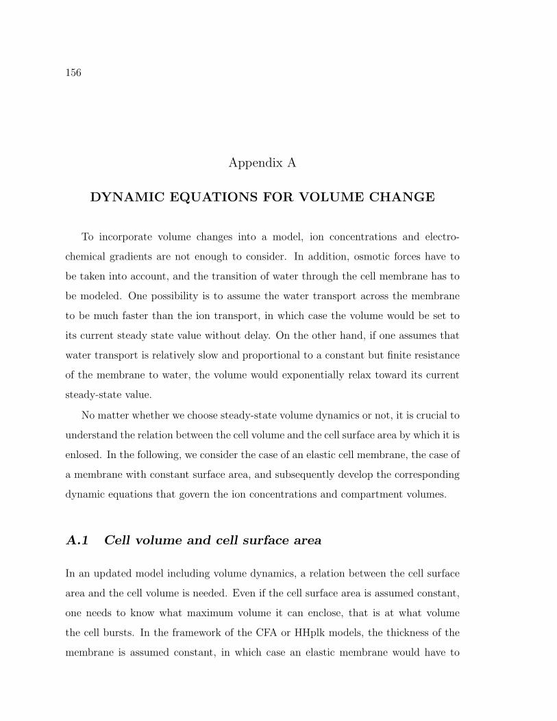
156
Appendix A
DYNAMIC EQUATIONS FOR VOLUME CHANGE
To incorporate volume changes into a model, ion concentrations and electro-
chemical gradients are not enough to consider. In addition, osmotic forces have to
be taken into account, and the transition of water through the cell membrane has to
be modeled. One possibility is to assume the water transport across the membrane
to be much faster than the ion transport, in which case the volume would be set to
its current steady state value without delay. On the other hand, if one assumes that
water transport is relatively slow and proportional to a constant but finite resistance
of the membrane to water, the volume would exponentially relax toward its current
steady-state value.
No matter whether we choose steady-state volume dynamics or not, it is crucial to
understand the relation between the cell volume and the cell surface area by which it is
enlosed. In the following, we consider the case of an elastic cell membrane, the case of
a membrane with constant surface area, and subsequently develop the corresponding
dynamic equations that govern the ion concentrations and compartment volumes.
A.1 Cell volume and cell surface area
In an updated model including volume dynamics, a relation between the cell surface
area and the cell volume is needed. Even if the cell surface area is assumed constant,
one needs to know what maximum volume it can enclose, that is at what volume
the cell bursts. In the framework of the CFA or HHplk models, the thickness of the
membrane is assumed constant, in which case an elastic membrane would have to
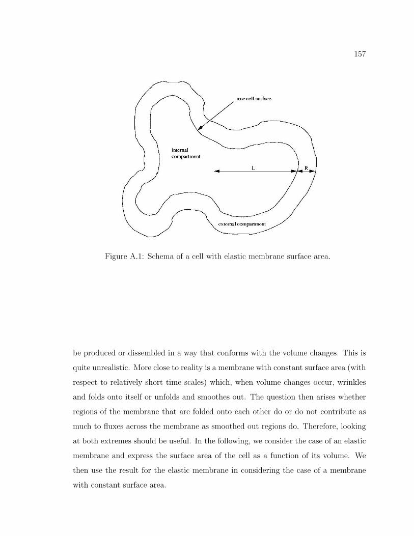
157
Figure A.1: Schema of a cell with elastic membrane surface area.
be produced or dissembled in a way that conforms with the volume changes. This is
quite unrealistic. More close to reality is a membrane with constant surface area (with
respect to relatively short time scales) which, when volume changes occur, wrinkles
and folds onto itself or unfolds and smoothes out. The question then arises whether
regions of the membrane that are folded onto each other do or do not contribute as
much to fluxes across the membrane as smoothed out regions do. Therefore, looking
at both extremes should be useful. In the following, we consider the case of an elastic
membrane and express the surface area of the cell as a function of its volume. We
then use the result for the elastic membrane in considering the case of a membrane
with constant surface area.
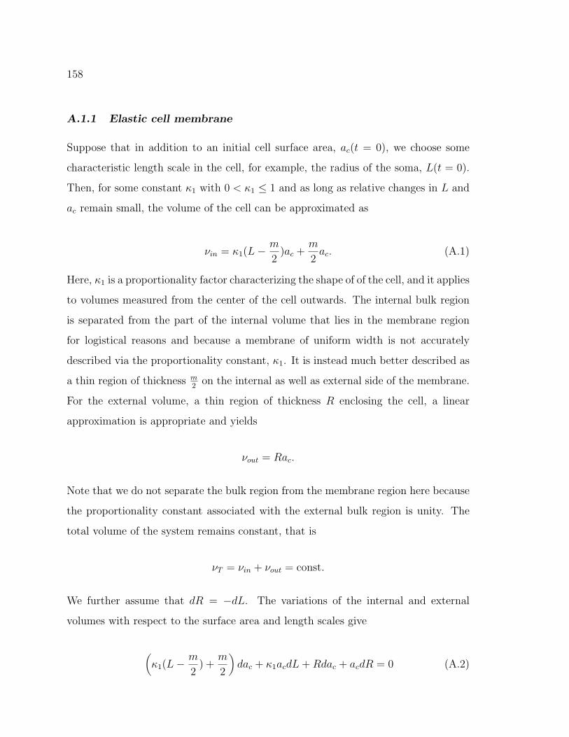
158
A.1.1 Elastic cell membrane
Suppose that in addition to an initial cell surface area, ac(t = 0), we choose some
characteristic length scale in the cell, for example, the radius of the soma, L(t = 0).
Then, for some constant κ1 with 0 < κ1 ≤ 1 and as long as relative changes in L and
ac remain small, the volume of the cell can be approximated as
νin = κ1(L−m
2)ac +
m
2ac. (A.1)
Here, κ1 is a proportionality factor characterizing the shape of of the cell, and it applies
to volumes measured from the center of the cell outwards. The internal bulk region
is separated from the part of the internal volume that lies in the membrane region
for logistical reasons and because a membrane of uniform width is not accurately
described via the proportionality constant, κ1. It is instead much better described as
a thin region of thickness m2
on the internal as well as external side of the membrane.
For the external volume, a thin region of thickness R enclosing the cell, a linear
approximation is appropriate and yields
νout = Rac.
Note that we do not separate the bulk region from the membrane region here because
the proportionality constant associated with the external bulk region is unity. The
total volume of the system remains constant, that is
νT = νin + νout = const.
We further assume that dR = −dL. The variations of the internal and external
volumes with respect to the surface area and length scales give
(κ1(L−
m
2) +
m
2
)dac + κ1acdL + Rdac + acdR = 0 (A.2)
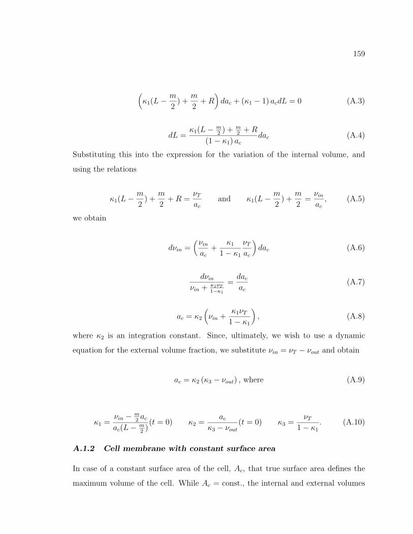
159
(κ1(L−
m
2) +
m
2+ R
)dac + (κ1 − 1) acdL = 0 (A.3)
dL =κ1(L− m
2) + m
2+ R
(1− κ1) ac
dac (A.4)
Substituting this into the expression for the variation of the internal volume, and
using the relations
κ1(L−m
2) +
m
2+ R =
νT
ac
and κ1(L−m
2) +
m
2=
νin
ac
, (A.5)
we obtain
dνin =(
νin
ac
+κ1
1− κ1
νT
ac
)dac (A.6)
dνin
νin + κ1νT
1−κ1
=dac
ac
(A.7)
ac = κ2
(νin +
κ1νT
1− κ1
), (A.8)
where κ2 is an integration constant. Since, ultimately, we wish to use a dynamic
equation for the external volume fraction, we substitute νin = νT − νout and obtain
ac = κ2 (κ3 − νout) , where (A.9)
κ1 =νin − m
2ac
ac(L− m2)(t = 0) κ2 =
ac
κ3 − νout
(t = 0) κ3 =νT
1− κ1
. (A.10)
A.1.2 Cell membrane with constant surface area
In case of a constant surface area of the cell, Ac, that true surface area defines the
maximum volume of the cell. While Ac = const., the internal and external volumes
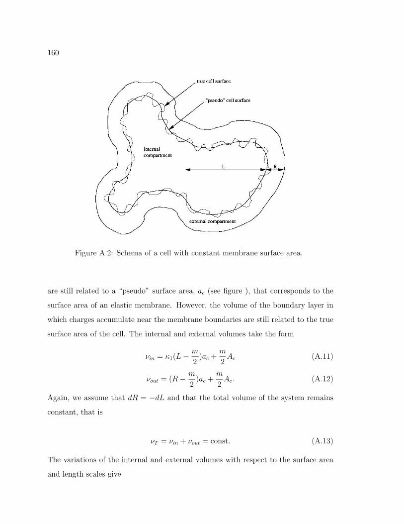
160
Figure A.2: Schema of a cell with constant membrane surface area.
are still related to a “pseudo” surface area, ac (see figure ), that corresponds to the
surface area of an elastic membrane. However, the volume of the boundary layer in
which charges accumulate near the membrane boundaries are still related to the true
surface area of the cell. The internal and external volumes take the form
νin = κ1(L−m
2)ac +
m
2Ac (A.11)
νout = (R− m
2)ac +
m
2Ac. (A.12)
Again, we assume that dR = −dL and that the total volume of the system remains
constant, that is
νT = νin + νout = const. (A.13)
The variations of the internal and external volumes with respect to the surface area
and length scales give
161
κ1(L−m
2)dac + κ1acdL + (R− m
2)dac + acdR = 0 (A.14)
(κ1(L−
m
2) + R− m
2
)dac + (κ1 − 1) acdL = 0 (A.15)
dL =κ1(L− m
2) + R− m
2
(1− κ1) ac
dac (A.16)
Substituting this into the expression for the variation of the internal volume and using
that
κ1(L−m
2) + R− m
2=
νT − 2m2Ac
ac
and κ1(L−m
2) =
νin − m2Ac
ac
(A.17)
we obtain
dνin =
(νin − m
2Ac
ac
+κ1
1− κ1
νT − 2m2Ac
ac
)dac (A.18)
dνin
νin + κ1νT
1−κ1− m
2Ac
1+κ1
1−κ1
=dac
ac
(A.19)
ac = κ2
(νin +
κ1νT
1− κ1
− m
2Ac
1 + κ1
1− κ1
), (A.20)
where κ2 is an integration constant. Since, ultimately, we wish to use a dynamic
equation for the external volume fraction, we substitute νin = νT − νout and obtain
ac = κ2 (κ3 − νout) , where (A.21)
κ1 =νin − m
2Ac
ac(L− m2)(t = 0) κ2 =
ac
κ3 − νout
(t = 0) κ3 =νT
1− κ1
− m
2Ac
1 + κ1
1− κ1
(A.22)
162
One could choose ac(t = 0) = Ac but this would imply that the initial volume was the
maximum volume. One should much rather choose all initial values from characteristic
measurements of appropriate cells and define the total volume and constants, κ1,2,3,
as far as possible. Recall that κ1,3 are dependent on Ac. Afterwards, decide on a
maximum volume of the cell, for example, relative to the total volume, and define by
it the constant surface area by solving Ac = κ2
(κ3(Ac)− ν
(min)out
)for Ac.
A.2 Cell volume dynamics
The volume of a cell changes due to the passage of water from one side of its membrane
to the other. This migration of water is driven by an osmotic pressure gradient across
the membrane, which in turn is caused by a difference in osmolar (total particle)
concentrations from one side of the membrane to the other. In sufficiently dilute
systems, the osmotic pressure is directly proportional to the osmolar concentration
gradient across the membrane, that is
d
dtνout = G0
∑i
couti − cin
i , (A.23)
where cin,outi denote the average internal and external concentrations of species i,
respectively. Any trapped species are included in the summation. The proportionality
factor, G0, is related to the permeability of the cell membrane to water, and dependent
on the cell surface area. For a detailed derivation of the exact form of G0, please refer
to section B.1 on the incorporation of HH-style fluxes and pumps. Meanwhile, we
state that in the case of a constant surface area of the cell, Ac,
d
dtνout =
Ac
ηHH2O
(∑i
couti − cin
i
)(A.24)
and in the case of an elastic membrane,
163
d
dtνout =
κ2
ηHH2O (κ3 − νout)
(∑i
couti − cin
i
), (A.25)
where HH2O is the permeability of the membrane to water per unit width, η is a
conversion factor for units, and κ2,3 are integration constants that arise when the
elastic membrane surface area is expressed in terms of the volume it encloses.
A.3 Concentration dynamics
From any given set of internal concentrations, cini , and cell volume, vin, we can now
define the external concentrations, couti , and volume, vout, the cross-membrane po-
tential, ∆ϕ = − FVR0T
, the net flux densities, Ji, and the pseudo cell surface area, ac.
To obtain ODEs in time for the bulk concentrations that take volume changes into
account, we begin with a particular version of the continuity equation,
d
dt
(vinc
ini
)= −AcJi , (A.26)
where the boundary corresponding to the left end of the domain satisfies a zero flux
condition, ensuring mass conservation. Ac denotes the true cell surface area and may
be constant or, in the case of an elastic cell membrane, may equal the pseudo cell
surface area, ac. Note that this implies that, at this point, all regions of the cell
surface area contribute equally to the flux across it, even when regions of a constant
membrane surface that are folded onto each other. Using the product rule, we obtain
dvin
dt· cin
i + vin ·dcin
i
dt= −AcJi (A.27)
vin ·dcin
i
dt= −AcJi −
dvin
dt· cin
i (A.28)
vin ·dcin
i
dt= −AcJi +
dvout
dt· cin
i , (A.29)
where we have used that dvin
dt= −dvout
dt. dvout
dtis given by (A.24) in case of constant
cell surface area and by (A.25) in case of and elastic cell membrane. Recall that Ac

164
denotes the true cell surface area and may be constant or, in the case of an elastic
cell membrane, may equal the pseudo cell surface area, ac.
165
Appendix B
MODELING SOPHISTICATED CHANNELS AND
ACTIVE TRANSPORT
Any living cell employs an intricate machinery of proteins embedded in its mem-
brane that maintains ion concentrations within preferred ranges and, in particular,
far away from equilibrium. In order to observe any of the dynamics of the cross-
membrane potential typical for neurons, we have to incorporate models for the fluxes
through certain parts of the cell’s protein machinery.
B.1 Channels and Pumps in the CFA framework
There is a large literature on ion pump and ion channel fluxes in HH-style models.
To make use of this rich source, our goal is to establish how any HH-style flux can be
incorporated into the model framework of the CFA. The issue here is not to match
HH-type conductances with diffusion coefficients, this was done in section 4.3, but
rather how to move toward using biophysically relevant and consistent parameters
instead of parameters that were fit to data after assuming a form of the solution.
Making this transition is important in determining whether a model has taken into
account the components necessary for a good, qualitative and quantitative prediction.
We begin by considering diffusive fluxes, distinguish two cases, and consider both of
them consecutively:
1. The membrane is a lipid bilayer, in which case we need a diffusion constant
valid inside a cell membrane. This will be the case for leak fluxes through the
membrane.
166
2. We treat a channel through the membrane as a solute-filled pore. In this case,
we need a diffusion constant valid in a solute-filled pore across which there is a
potential difference.
B.1.1 Diffusion coefficients in lipid membrane
In this section, based on cell membrane permeabilities to various ion species, we define
diffusion constants valid throughout the membrane. Since the passive, diffusive fluxes
through cell membrane are not related to ion channels, we are looking at leak fluxes,
which the CFA defines via a GHK-type equation.
From the physical point of view, the diffusion in the internal and external com-
partments is very fast compared to the diffusion through the membrane. Therefore,
the diffusion through the region formed by boundary layer and membrane combined
is limited by the diffusion through the membrane. An “effective” diffusion constant
describing the diffusion through any external boundary layer and membrane would
therefore approximately equal the diffusion constant for lipid membrane and involve
the true width of the lipid membrane.
From a mathematical point of view, we have assumed that the width of the mem-
brane equals the width of any internal boundary layers. It was demonstrated in
subsection 2.1.1 that the width of the boundary layer is very similar to the true width
of the lipid membrane. Therefore, the effective diffusion constant from physical con-
siderations is approximately the same as the one from mathematical considerations.
In introductory literature of biochemistry, we find measurements of permeability
coefficients, Hi, for human erythrocyte membrane for various ionic species, i. Their
values express a diffusion constant per unit width of membrane and are given in units
of ms
in table B.1.1. The units of the diffusion constant, [Di] = m2
s. By using the
width of the boundary layer as width of the cell membrane as established elsewhere,
we can define the diffusion constants in CFA by
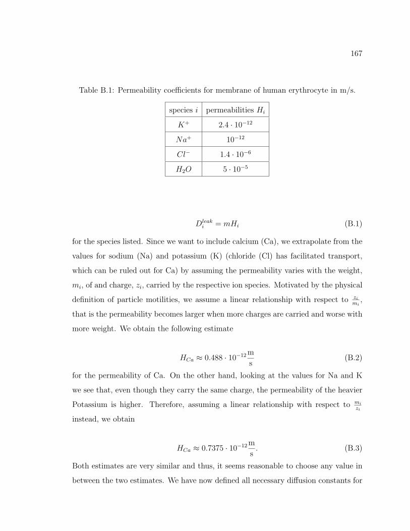
167
Table B.1: Permeability coefficients for membrane of human erythrocyte in m/s.
species i permeabilities Hi
K+ 2.4 · 10−12
Na+ 10−12
Cl− 1.4 · 10−6
H2O 5 · 10−5
Dleaki = mHi (B.1)
for the species listed. Since we want to include calcium (Ca), we extrapolate from the
values for sodium (Na) and potassium (K) (chloride (Cl) has facilitated transport,
which can be ruled out for Ca) by assuming the permeability varies with the weight,
mi, of and charge, zi, carried by the respective ion species. Motivated by the physical
definition of particle motilities, we assume a linear relationship with respect to zi
mi,
that is the permeability becomes larger when more charges are carried and worse with
more weight. We obtain the following estimate
HCa ≈ 0.488 · 10−12 m
s(B.2)
for the permeability of Ca. On the other hand, looking at the values for Na and K
we see that, even though they carry the same charge, the permeability of the heavier
Potassium is higher. Therefore, assuming a linear relationship with respect to mi
zi
instead, we obtain
HCa ≈ 0.7375 · 10−12 m
s. (B.3)
Both estimates are very similar and thus, it seems reasonable to choose any value in
between the two estimates. We have now defined all necessary diffusion constants for
168
the purpose of computing leak fluxes. Furthermore, we have a value for the permeabil-
ity of a lipid membrane to water, which allows us to determine the proportionality
coefficient, G0, in the ODE governing volume changes (see appendix A). The leak
fluxes through the cell membrane are defined in CFA by a GHK-type equation,
J leaki = −Dleak
i
zi∆ϕ
m· cout
i ezi∆ϕ − cini
ezi∆ϕ − 1, (B.4)
where cin,outi denote the average internal and external concentrations of species i and
∆ϕ is the cross-membrane potential difference.
B.1.2 Diffusion coefficients in solute filled pores
In this section, we use a linear current voltage relationship that is valid in a sig-
nificantly dilute electrolyte solution. Using this relationship, we define the diffusion
coefficient for an electrolyte filled pore in the cell membrane, across which there is a
non-zero potential difference. This approach may be justified by considering that the
total flux across the pore due to a concentration gradient and an electro-static poten-
tial gradient is related to both gradients by the same diffusion constant. Therefore,
we assume that the value obtained for the case of just a potential gradient can also
be used for the case of both a potential and a concentration gradient. After it has
been computed, the diffusion coefficient for an electrolyte filled pore is related to the
maximum flux through a particular type of ion channel via the generalized GHK-type
equation, and the appropriate gating variables lead to the average channel flux.
Consider an ion channel as a solute filled pore of length m = 2√
ε. Further, suppose
that, in case of a constant membrane surface area, the fraction of the membrane
surface occupied by the considered type of channels is Achan
Ac. For a significantly dilute
system, the conductivity, G, of a region of electrolyte of the above dimensions linearly
relates a current, I, in units of Ampere to a potential difference, U , in units of Volt
across the pore,
169
I = GU.
In our case, the absolute current is I = ziFAcJi for ion species i, the absolute potential
difference is U = −R0TF
∆ϕ, and the conductivity with respect to ion species i is
G = ΓiciAchan
m, (B.5)
where ci is the (supposedly homogeneous) concentration of species i in the channel
pore and Γi is called the “equivalent conductivity” for species i and is given in units
of m2
Ωmol. Substituting the expressions for I, U , and G into the linear relationship, and
solving for the flux density, Ji, in units of molm2s
consistent with our model fluxes, we
obtain
Ji = −ΓiAchanR0T
ziF 2Ac
ci∆ϕ
m. (B.6)
Comparing (B.6) with the ionic flux of species i with valency zi and concentration ci
due to a local electric field ∇ϕ,
Ji = −ziDici∇ϕ (B.7)
≈ −ziDici∆ϕ
m. (B.8)
Comparing (B.6) and (B.8), we find that the appropriate diffusion constant, which
is related to the flux of species i through channels of the considered type when all
channels are open, is
Dchani =
ΓiAchanR0T
z2i F
2Ac
. (B.9)
We have neglected in this derivation that, in addition to a potential gradient across
the pore, we also have a concentration gradient. However, in case of a non-negligible
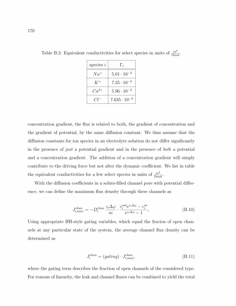
170
Table B.2: Equivalent conductivities for select species in units of m2
Ωmol.
species i Γi
Na+ 5.01 · 10−3
K+ 7.35 · 10−3
Ca2+ 5.96 · 10−3
Cl− 7.635 · 10−3
concentration gradient, the flux is related to both, the gradient of concentration and
the gradient of potential, by the same diffusion constant. We thus assume that the
diffusion constants for ion species in an electrolyte solution do not differ significantly
in the presence of just a potential gradient and in the presence of both a potential
and a concentration gradient. The addition of a concentration gradient will simply
contribute to the driving force but not alter the dynamic coefficient. We list in table
the equivalent conductivities for a few select species in units of m2
Ωmol.
With the diffusion coefficients in a solute-filled channel pore with potential differ-
ence, we can define the maximum flux density through these channels as
J chani,max = −Dchan
i
zi∆ϕ
m· cout
i ezi∆ϕ − cini
ezi∆ϕ − 1, (B.10)
Using appropriate HH-style gating variables, which equal the fracion of open chan-
nels at any particular state of the system, the average channel flux density can be
determined as
J chani = (gating) · J chan
i,max, (B.11)
where the gating term describes the fraction of open channels of the considered type.
For reasons of linearity, the leak and channel fluxes can be combined to yield the total
171
passive flux density of species i,
Jpassi = J leak
i + J chani = −
(Dleak
i + (gating) ·Dchani
) zi∆ϕ
m· cout
i ezi∆ϕ − cini
ezi∆ϕ − 1. (B.12)
Note that in the presence of multiple channel types for one species, the individual
channel flux densities may simply be superimposed an yield
Jpassi = −
(Dleak
i +∑k
(gating)chan k ·Dchan ki
)zi∆ϕ
m· cout
i ezi∆ϕ − cini
ezi∆ϕ − 1. (B.13)
B.1.3 Pump fluxes
Channel as well as leak fluxes are passive, that is they flow down their electro-chemical
gradient. In the following, we consider active pump fluxes, which correspond to
the transported of species across the cell membrane against their electro-chemical
gradient. In literature, pump fluxes have most simply been modeled by sigmoidal
functions. For example, Murray [52], Falcke et al. [18], and Shorten and Wall [73] use
Jpump = ± σ1cn
cn + σn2
(B.14)
for various pump and exchanger fluxes. Here, σ1 is the maximum capacity of the
pump, σ2 is the concentration at which the pump works at half capacity, c is the
concentration of an ion species in the compartment from which it is expelled, and the
sign indicates whether a species is expelled from the internal or external compartment.
The Hill coefficient, n, is usually and integer ranging from 1 to 4, is determined by fit
to data, and indicates the sensitivity of the pump to the concentration, c. As a rule
of thumb, one can say that the larger the Hill coefficient, the steeper the response of
the pump.
If pump fluxes of sigmoidal type are in units of mols
, that is particles per unit time,
they can be converted to flux densities by simply dividing them by the membrane
172
surface area, Ac, or by redefining σ1 = σ1
Ac. The resulting pump flux density for species
i has the same form as in (B.14). If pump fluxes of sigmoidal type are instead in units
of molm3s
, that is concentration per unit time, they can be converted to flux densities by
multiplying by the volume of the compartment from which they expel a species and
by dividing by the membrane surface area, Ac. The simplest way to implement this
is to redefine σ1 = νσ1
Ac, for an appropriate volume, ν, and the pump flux takes the
same form as in (B.14).
A problem potentially arises when the model includes compartments whose vol-
umes vary with time. Multiplying a flux in units of concentration per unit time by a
volume defines a flux in units of particles per unit time. However, the HH-type model
from which the flux originates relies on fixed volumes, that is the related particle
flux may only be valid for this one, particular, fixed volume. The question remains
whether, for relatively small volume changes, one should use a fixed volume (initial
volume) as a conversion factor or whether the use of the true, time dependent, volume
is more appropriate. Once this difficulty is overcome, the net flux density of species
i,
JTi = Jpass
i + Jpumpi = J leak
i + J chani + Jpump
i . (B.15)
The total flux of particles of species i from the internal to the external compartment
is simply AcJTi , which is responsible for concentration dynamics.
B.1.4 Calcium sensitivity
Calcium (Ca) plays an important role in intra- and inter-cellular signaling and has
been linked to the synchronization of cell networks, cicadian rhythms, and more [52].
Thus, it is not surprising that Ca has a significant influence on some concentration-
dependent ion fluxes, such as the one through the Ca-dependent K channel. It also
participates in its own regulation by a feedback mechanism called Ca-induced Ca
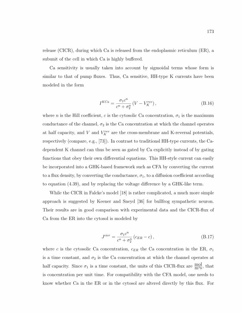
173
release (CICR), during which Ca is released from the endoplasmic reticulum (ER), a
subunit of the cell in which Ca is highly buffered.
Ca sensitivity is usually taken into account by sigmoidal terms whose form is
similar to that of pump fluxes. Thus, Ca sensitive, HH-type K currents have been
modeled in the form
IKCa =σ1c
n
cn + σn2
(V − V revK ) , (B.16)
where n is the Hill coefficient, c is the cytosolic Ca concentration, σ1 is the maximum
conductance of the channel, σ2 is the Ca concentration at which the channel operates
at half capacity, and V and V revK are the cross-membrane and K-reversal potentials,
respectively (compare, e.g., [73]). In contrast to traditionsl HH-type currents, the Ca-
dependent K channel can thus be seen as gated by Ca explicitly instead of by gating
functions that obey their own differential equations. This HH-style current can easily
be incorporated into a GHK-based framework such as CFA by converting the current
to a flux density, by converting the conductance, σ1, to a diffusion coefficient according
to equation (4.39), and by replacing the voltage difference by a GHK-like term.
While the CICR in Falcke’s model [18] is rather complicated, a much more simple
approach is suggested by Keener and Sneyd [36] for bullfrog sympathetic neuron.
Their results are in good comparison with experimental data and the CICR-flux of
Ca from the ER into the cytosol is modeled by
J cicr =σ1c
n
cn + σn2
(cER − c) , (B.17)
where c is the cytosolic Ca concentration, cER the Ca concentration in the ER, σ1
is a time constant, and σ2 is the Ca concentration at which the channel operates at
half capacity. Since σ1 is a time constant, the units of this CICR-flux are molm3s , that
is concentration per unit time. For compatibility with the CFA model, one needs to
know whether Ca in the ER or in the cytosol are altered directly by this flux. For

174
example, if cytosolic Ca is affected directly, then
dc
dt= J cicr and (B.18)
dcER
dt= − vin
vER
J cicr, (B.19)
where vin and vcicr denote the cytosolic and ER volumes, respectively. CICR is,
however, not solely dependent on Ca concentrations but also mediated by high- and
low-voltage activated channels and by channels sensitive to IP3, a secondary messen-
ger. Working against its gradient, Ca is also continuously expelled from the cytosol
by ion pumps that transport Ca into the ER or out of the cell. The latter is, among
other means, achieved by the Na-Ca exchanger, which exploits the Na gradient to
“lift” Ca out of the cytosol. We shall not explore CICR any further since there is a
large literature on it and attempting to give a concise overview would be inappropriate
within the frame of this work.
B.1.5 Volume dynamics via flux of water
The volume of a cell changes due to the passage of water from one side of its membrane
to the other. This migration of water is driven by an osmotic pressure gradient across
the membrane, which in turn is caused by a difference in osmolar (total particle)
concentrations from one side of the membrane to the other. In sufficiently dilute
systems, the osmotic pressure is directly proportional to the osmolar concentration
gradient across the membrane.
We assume in the following that the osmotic pressure difference across the mem-
brane is the sole driving force behind the flux of water across the membrane. Thus,
the rate of change of volume is directly proportional to the osmolar concentration
difference across the membrane and boundary layer. Due to the assumed proportion-
ality, we describe the flux of water through the membrane as a diffusion-type process
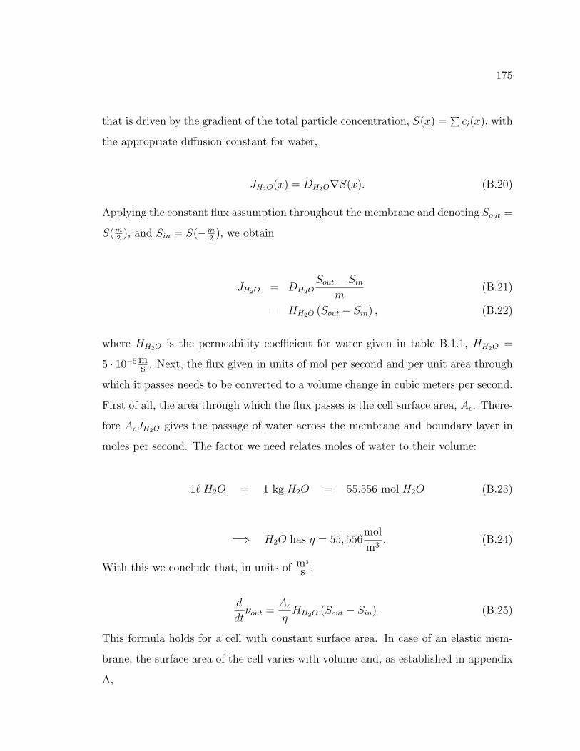
175
that is driven by the gradient of the total particle concentration, S(x) =∑
ci(x), with
the appropriate diffusion constant for water,
JH2O(x) = DH2O∇S(x). (B.20)
Applying the constant flux assumption throughout the membrane and denoting Sout =
S(m2), and Sin = S(−m
2), we obtain
JH2O = DH2OSout − Sin
m(B.21)
= HH2O (Sout − Sin) , (B.22)
where HH2O is the permeability coefficient for water given in table B.1.1, HH2O =
5 · 10−5 ms . Next, the flux given in units of mol per second and per unit area through
which it passes needs to be converted to a volume change in cubic meters per second.
First of all, the area through which the flux passes is the cell surface area, Ac. There-
fore AcJH2O gives the passage of water across the membrane and boundary layer in
moles per second. The factor we need relates moles of water to their volume:
1` H2O = 1 kg H2O = 55.556 mol H2O (B.23)
=⇒ H2O has η = 55, 556mol
m3. (B.24)
With this we conclude that, in units of m3
s ,
d
dtνout =
Ac
ηHH2O (Sout − Sin) . (B.25)
This formula holds for a cell with constant surface area. In case of an elastic mem-
brane, the surface area of the cell varies with volume and, as established in appendix
A,
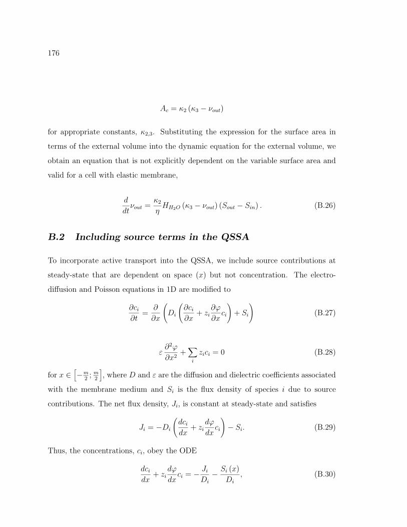
176
Ac = κ2 (κ3 − νout)
for appropriate constants, κ2,3. Substituting the expression for the surface area in
terms of the external volume into the dynamic equation for the external volume, we
obtain an equation that is not explicitly dependent on the variable surface area and
valid for a cell with elastic membrane,
d
dtνout =
κ2
ηHH2O (κ3 − νout) (Sout − Sin) . (B.26)
B.2 Including source terms in the QSSA
To incorporate active transport into the QSSA, we include source contributions at
steady-state that are dependent on space (x) but not concentration. The electro-
diffusion and Poisson equations in 1D are modified to
∂ci
∂t=
∂
∂x
(Di
(∂ci
∂x+ zi
∂ϕ
∂xci
)+ Si
)(B.27)
ε∂2ϕ
∂x2+∑
i
zici = 0 (B.28)
for x ∈[−m
2; m
2
], where D and ε are the diffusion and dielectric coefficients associated
with the membrane medium and Si is the flux density of species i due to source
contributions. The net flux density, Ji, is constant at steady-state and satisfies
Ji = −Di
(dci
dx+ zi
dϕ
dxci
)− Si. (B.29)
Thus, the concentrations, ci, obey the ODE
dci
dx+ zi
dϕ
dxci = − Ji
Di
− Si (x)
Di
, (B.30)
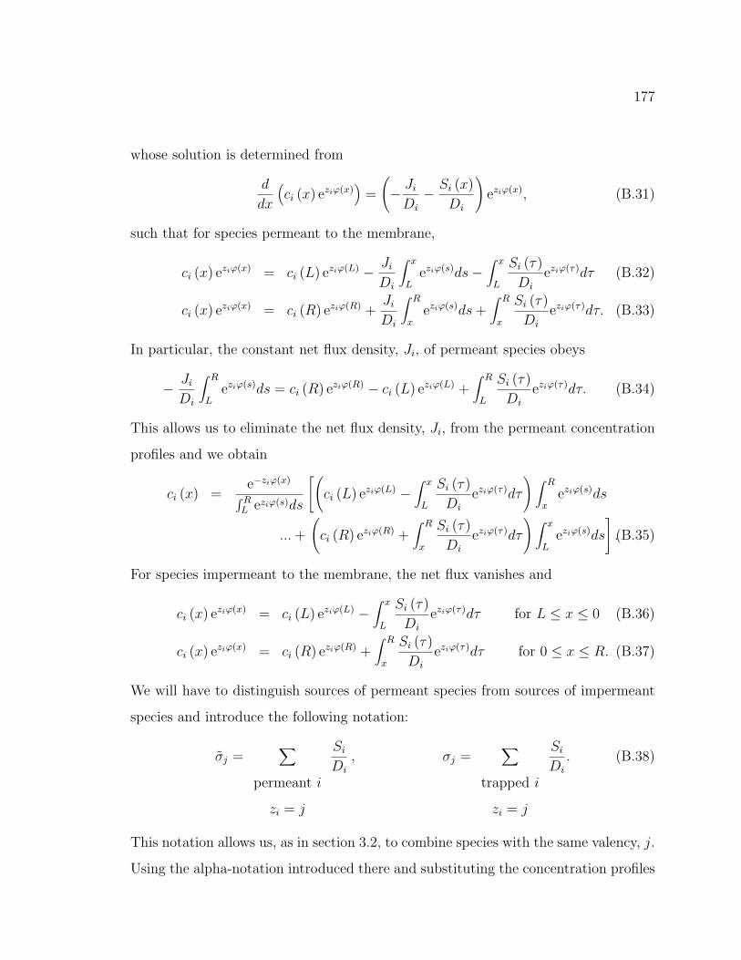
177
whose solution is determined from
d
dx
(ci (x) eziϕ(x)
)=
(− Ji
Di
− Si (x)
Di
)eziϕ(x), (B.31)
such that for species permeant to the membrane,
ci (x) eziϕ(x) = ci (L) eziϕ(L) − Ji
Di
∫ x
Leziϕ(s)ds−
∫ x
L
Si (τ)
Di
eziϕ(τ)dτ (B.32)
ci (x) eziϕ(x) = ci (R) eziϕ(R) +Ji
Di
∫ R
xeziϕ(s)ds +
∫ R
x
Si (τ)
Di
eziϕ(τ)dτ. (B.33)
In particular, the constant net flux density, Ji, of permeant species obeys
− Ji
Di
∫ R
Leziϕ(s)ds = ci (R) eziϕ(R) − ci (L) eziϕ(L) +
∫ R
L
Si (τ)
Di
eziϕ(τ)dτ. (B.34)
This allows us to eliminate the net flux density, Ji, from the permeant concentration
profiles and we obtain
ci (x) =e−ziϕ(x)∫ R
L eziϕ(s)ds
[(ci (L) eziϕ(L) −
∫ x
L
Si (τ)
Di
eziϕ(τ)dτ
)∫ R
xeziϕ(s)ds
... +
(ci (R) eziϕ(R) +
∫ R
x
Si (τ)
Di
eziϕ(τ)dτ
)∫ x
Leziϕ(s)ds
].(B.35)
For species impermeant to the membrane, the net flux vanishes and
ci (x) eziϕ(x) = ci (L) eziϕ(L) −∫ x
L
Si (τ)
Di
eziϕ(τ)dτ for L ≤ x ≤ 0 (B.36)
ci (x) eziϕ(x) = ci (R) eziϕ(R) +∫ R
x
Si (τ)
Di
eziϕ(τ)dτ for 0 ≤ x ≤ R. (B.37)
We will have to distinguish sources of permeant species from sources of impermeant
species and introduce the following notation:
σj =∑
permeant i
zi = j
Si
Di
, σj =∑
trapped i
zi = j
Si
Di
. (B.38)
This notation allows us, as in section 3.2, to combine species with the same valency, j.
Using the alpha-notation introduced there and substituting the concentration profiles
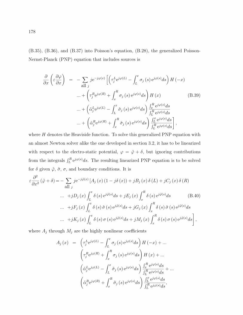
178
(B.35), (B.36), and (B.37) into Poisson’s equation, (B.28), the generalized Poisson-
Nernst-Planck (PNP) equation that includes sources is
∂
∂x
(ε∂ϕ
∂x
)= −
∑all j
je−jϕ(x)[(
τLj ejϕ(L) −
∫ x
Lσj (s) ejϕ(s)ds
)H (−x)
... +
(τRj ejϕ(R) +
∫ R
xσj (s) ejϕ(s)ds
)H (x) (B.39)
... +(αL
j ejϕ(L) −∫ x
Lσj (s) ejϕ(s)ds
) ∫ Rx ejϕ(s)ds∫ RL ejϕ(s)ds
... +
(αR
j ejϕ(R) +∫ R
xσj (s) ejϕ(s)ds
) ∫ xL ejϕ(s)ds∫ RL ejϕ(s)ds
],
where H denotes the Heaviside function. To solve this generalized PNP equation with
an almost Newton solver alike the one developed in section 3.2, it has to be linearized
with respect to the electro-static potential, ϕ = ϕ + δ, but ignoring contributions
from the integrals∫ RL ejϕ(s)ds. The resulting linearized PNP equation is to be solved
for δ given ϕ, σ, σ, and boundary conditions. It is
ε∂2
∂x2(ϕ + δ) =−
∑all j
je−jϕ(x) [Aj (x) (1− jδ (x)) + jBj (x) δ (L) + jCj (x) δ (R)
... +jDj (x)∫ x
Lδ (s) ejϕ(s)ds + jEj (x)
∫ R
xδ (s) ejϕ(s)ds (B.40)
... +jFj (x)∫ x
Lδ (s) σ (s) ejϕ(s)ds + jGj (x)
∫ R
xδ (s) σ (s) ejϕ(s)ds
... +jKj (x)∫ x
Lδ (s) σ (s) ejϕ(s)ds + jMj (x)
∫ R
xδ (s) σ (s) ejϕ(s)ds
],
where Aj through Mj are the highly nonlinear coefficients
Aj (x) =(τLj ejϕ(L) −
∫ x
Lσj (s) ejϕ(s)ds
)H (−x) + ...(
τRj ejϕ(R) +
∫ R
xσj (s) ejϕ(s)ds
)H (x) + ...
(αL
j ejϕ(L) −∫ x
Lσj (s) ejϕ(s)ds
) ∫ Rx ejϕ(s)ds∫ RL ejϕ(s)ds
+ ...(αR
j ejϕ(R) +∫ R
xσj (s) ejϕ(s)ds
) ∫ xL ejϕ(s)ds∫ RL ejϕ(s)ds
,
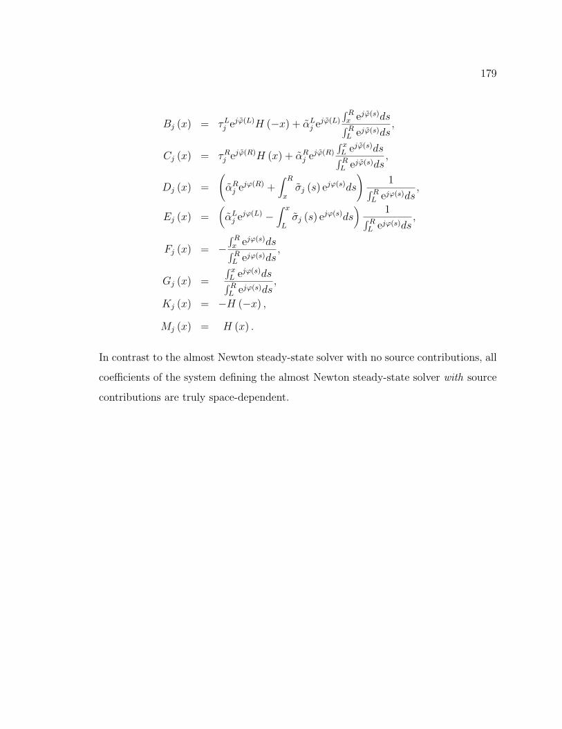
179
Bj (x) = τLj ejϕ(L)H (−x) + αL
j ejϕ(L)
∫ Rx ejϕ(s)ds∫ RL ejϕ(s)ds
,
Cj (x) = τRj ejϕ(R)H (x) + αR
j ejϕ(R)
∫ xL ejϕ(s)ds∫ RL ejϕ(s)ds
,
Dj (x) =
(αR
j ejϕ(R) +∫ R
xσj (s) ejϕ(s)ds
)1∫ R
L ejϕ(s)ds,
Ej (x) =(αL
j ejϕ(L) −∫ x
Lσj (s) ejϕ(s)ds
)1∫ R
L ejϕ(s)ds,
Fj (x) = −∫ Rx ejϕ(s)ds∫ RL ejϕ(s)ds
,
Gj (x) =
∫ xL ejϕ(s)ds∫ RL ejϕ(s)ds
,
Kj (x) = −H (−x) ,
Mj (x) = H (x) .
In contrast to the almost Newton steady-state solver with no source contributions, all
coefficients of the system defining the almost Newton steady-state solver with source
contributions are truly space-dependent.
180
Appendix C
EPILEPSY: AN INTRODUCTION
Epilepsy is a common neurological disorder. About 1% of humans are afflicted
by intermittently recurring seizures that, to this day, can at most be treated symp-
tomatically. The major difficulty lies in anticipating a seizure such that its occurrence
can be prevented. Clinical diagnosis, monitoring, and evaluation of the disease in a
patient is based on visual inspection of electroencephalogram (EEG) from scalp or
intra-cranial electrodes. Abundant clinical data is available from this source. On a
cellular level, hyper-synchronous, epileptic neural responses can be obtained by e.g.
enhancing synaptic excitability or enabling direct electrical field interactions between
neighboring soma. This suggests a more physical, rather than biological, basis of the
disorder. See [51] for an excellent overview of epilepsy, its pathology, and treatment
including the mathematical methods involved.
There exists a large literature on the physiological characterization and mathemat-
ical modeling of neural responses. Groundbreaking work was done by Hodgkin and
Huxley, who modeled dynamics of the potential difference across a membrane with
capacitance, and used current-voltage relations according to Ohm’s law, but with
varying conductances. Model equations for various ionic currents were based upon
the physiological knowledge of ion channels and plasma pumps in cell membranes at
the time and were fit to data from giant squid axon. Most of today’s literature is
closely related to this work and its assumptions.
For example, most Hodgkin and Huxley-type models today assume a cell with
fixed volume to be bathed in an infinitely buffered environment, causing volume and
interstitial concentrations not to change dynamically. This is appropriate for the
181
comparison and fit of data to in vitro slice studies since there, a thin slice of tissue
is bathed in a nourishing solution essentially fixing the cells’ environments. How-
ever, literature on epileptic neuron suggests that not only the dynamics of membrane
potential and cytosolic concentrations are of importance but also the dynamics of
interstitial concentrations and cell volume. A mathematical model including those
features will contribute to the understanding of the underlying mechanisms of epilep-
tic seizures and is a step toward being able to predict and prevent them. Therefore, a
suitable model for epileptic neuron cannot assume a cell with fixed volume immersed
in an infinite medium, as is the case for Hodgkin and Huxley.
C.1 Pathology and Medical Treatment
Epilepsy is the collective term for more than twenty different types of seizure disorders.
About 1% of humans are afflicted by recurring seizures, more than 2 million people
in the US. For half of the affected people, this common neurological condition starts
in childhood and many children just “grow out of it” before reaching adulthood. In
adults, epilepsy may have persisted from childhood or be the result of a head injury,
often caused by a car accident. The treatment of epilepsy to date does not result in
the complete restoration of a patient’s health but is restricted to reducing the visible
symptoms.
Seizure disorders take on several forms, depending upon where in the brain the
malfunction takes place, and how much of the total system is involved. Most people
think of generalized tonic clonic seizures when they hear the word “epilepsy”. In this
type of seizure, a person undergoes convulsions lasting a total of two to five minutes
with complete loss of consciousness and muscle spasms. On the other hand, absence
seizures appear as a blank stare and last for only a few seconds. Partial seizures
produce involuntary movements of an arm or a leg, distorted sensations, or a period
of automatic movement during which awareness is blurred or completely absent.
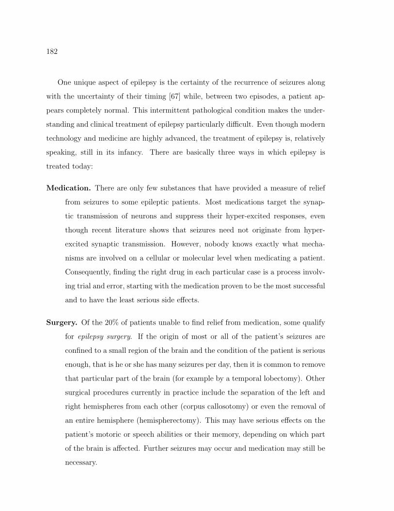
182
One unique aspect of epilepsy is the certainty of the recurrence of seizures along
with the uncertainty of their timing [67] while, between two episodes, a patient ap-
pears completely normal. This intermittent pathological condition makes the under-
standing and clinical treatment of epilepsy particularly difficult. Even though modern
technology and medicine are highly advanced, the treatment of epilepsy is, relatively
speaking, still in its infancy. There are basically three ways in which epilepsy is
treated today:
Medication. There are only few substances that have provided a measure of relief
from seizures to some epileptic patients. Most medications target the synap-
tic transmission of neurons and suppress their hyper-excited responses, even
though recent literature shows that seizures need not originate from hyper-
excited synaptic transmission. However, nobody knows exactly what mecha-
nisms are involved on a cellular or molecular level when medicating a patient.
Consequently, finding the right drug in each particular case is a process involv-
ing trial and error, starting with the medication proven to be the most successful
and to have the least serious side effects.
Surgery. Of the 20% of patients unable to find relief from medication, some qualify
for epilepsy surgery. If the origin of most or all of the patient’s seizures are
confined to a small region of the brain and the condition of the patient is serious
enough, that is he or she has many seizures per day, then it is common to remove
that particular part of the brain (for example by a temporal lobectomy). Other
surgical procedures currently in practice include the separation of the left and
right hemispheres from each other (corpus callosotomy) or even the removal of
an entire hemisphere (hemispherectomy). This may have serious effects on the
patient’s motoric or speech abilities or their memory, depending on which part
of the brain is affected. Further seizures may occur and medication may still be
necessary.
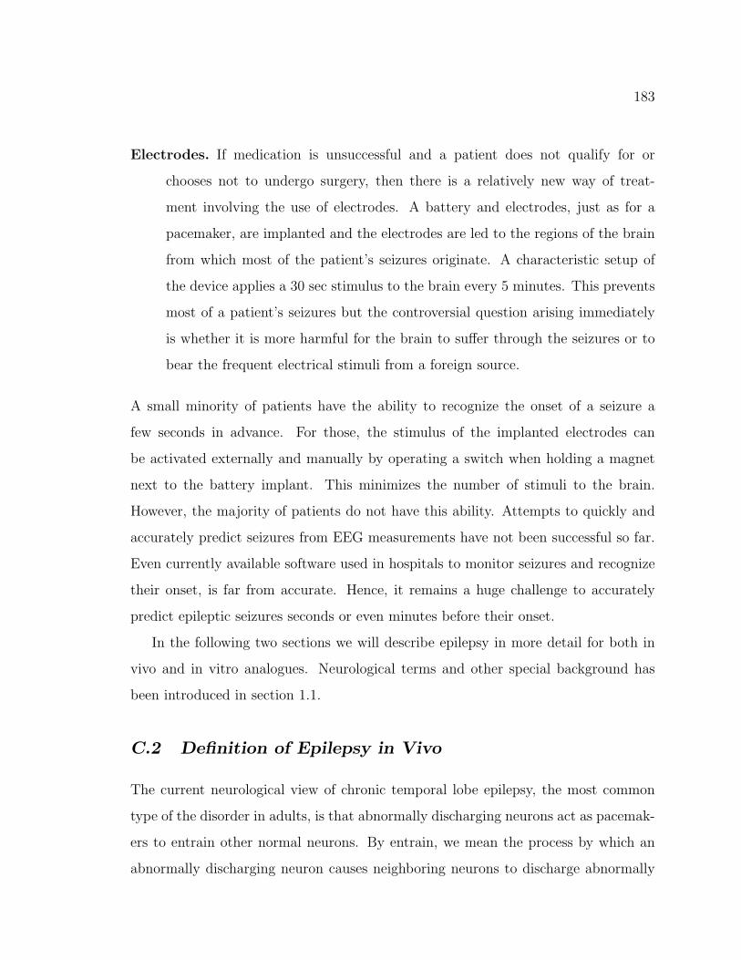
183
Electrodes. If medication is unsuccessful and a patient does not qualify for or
chooses not to undergo surgery, then there is a relatively new way of treat-
ment involving the use of electrodes. A battery and electrodes, just as for a
pacemaker, are implanted and the electrodes are led to the regions of the brain
from which most of the patient’s seizures originate. A characteristic setup of
the device applies a 30 sec stimulus to the brain every 5 minutes. This prevents
most of a patient’s seizures but the controversial question arising immediately
is whether it is more harmful for the brain to suffer through the seizures or to
bear the frequent electrical stimuli from a foreign source.
A small minority of patients have the ability to recognize the onset of a seizure a
few seconds in advance. For those, the stimulus of the implanted electrodes can
be activated externally and manually by operating a switch when holding a magnet
next to the battery implant. This minimizes the number of stimuli to the brain.
However, the majority of patients do not have this ability. Attempts to quickly and
accurately predict seizures from EEG measurements have not been successful so far.
Even currently available software used in hospitals to monitor seizures and recognize
their onset, is far from accurate. Hence, it remains a huge challenge to accurately
predict epileptic seizures seconds or even minutes before their onset.
In the following two sections we will describe epilepsy in more detail for both in
vivo and in vitro analogues. Neurological terms and other special background has
been introduced in section 1.1.
C.2 Definition of Epilepsy in Vivo
The current neurological view of chronic temporal lobe epilepsy, the most common
type of the disorder in adults, is that abnormally discharging neurons act as pacemak-
ers to entrain other normal neurons. By entrain, we mean the process by which an
abnormally discharging neuron causes neighboring neurons to discharge abnormally
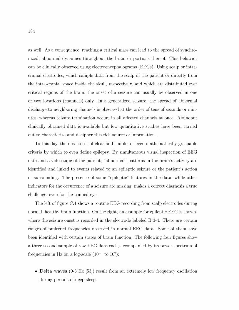
184
as well. As a consequence, reaching a critical mass can lead to the spread of synchro-
nized, abnormal dynamics throughout the brain or portions thereof. This behavior
can be clinically observed using electroencephalograms (EEGs). Using scalp or intra-
cranial electrodes, which sample data from the scalp of the patient or directly from
the intra-cranial space inside the skull, respectively, and which are distributed over
critical regions of the brain, the onset of a seizure can usually be observed in one
or two locations (channels) only. In a generalized seizure, the spread of abnormal
discharge to neighboring channels is observed at the order of tens of seconds or min-
utes, whereas seizure termination occurs in all affected channels at once. Abundant
clinically obtained data is available but few quantitative studies have been carried
out to characterize and decipher this rich source of information.
To this day, there is no set of clear and simple, or even mathematically graspable
criteria by which to even define epilepsy. By simultaneous visual inspection of EEG
data and a video tape of the patient, “abnormal” patterns in the brain’s activity are
identified and linked to events related to an epileptic seizure or the patient’s action
or surrounding. The presence of some “epileptic” features in the data, while other
indicators for the occurrence of a seizure are missing, makes a correct diagnosis a true
challenge, even for the trained eye.
The left of figure C.1 shows a routine EEG recording from scalp electrodes during
normal, healthy brain function. On the right, an example for epileptic EEG is shown,
where the seizure onset is recorded in the electrode labeled B 3-4. There are certain
ranges of preferred frequencies observed in normal EEG data. Some of them have
been identified with certain states of brain function. The following four figures show
a three second sample of raw EEG data each, accompanied by its power spectrum of
frequencies in Hz on a log-scale (10−1 to 102):
• Delta waves (0-3 Hz [53]) result from an extremely low frequency oscillation
during periods of deep sleep.
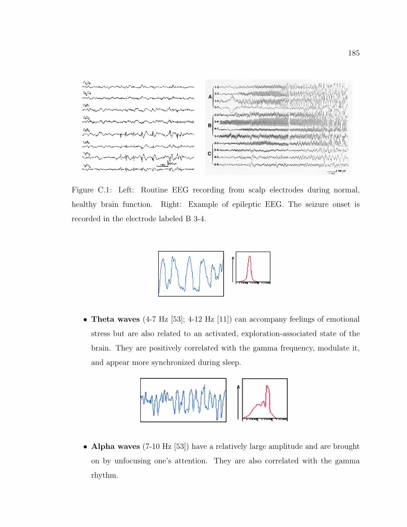
185
Figure C.1: Left: Routine EEG recording from scalp electrodes during normal,
healthy brain function. Right: Example of epileptic EEG. The seizure onset is
recorded in the electrode labeled B 3-4.
• Theta waves (4-7 Hz [53]; 4-12 Hz [11]) can accompany feelings of emotional
stress but are also related to an activated, exploration-associated state of the
brain. They are positively correlated with the gamma frequency, modulate it,
and appear more synchronized during sleep.
• Alpha waves (7-10 Hz [53]) have a relatively large amplitude and are brought
on by unfocusing one’s attention. They are also correlated with the gamma
rhythm.
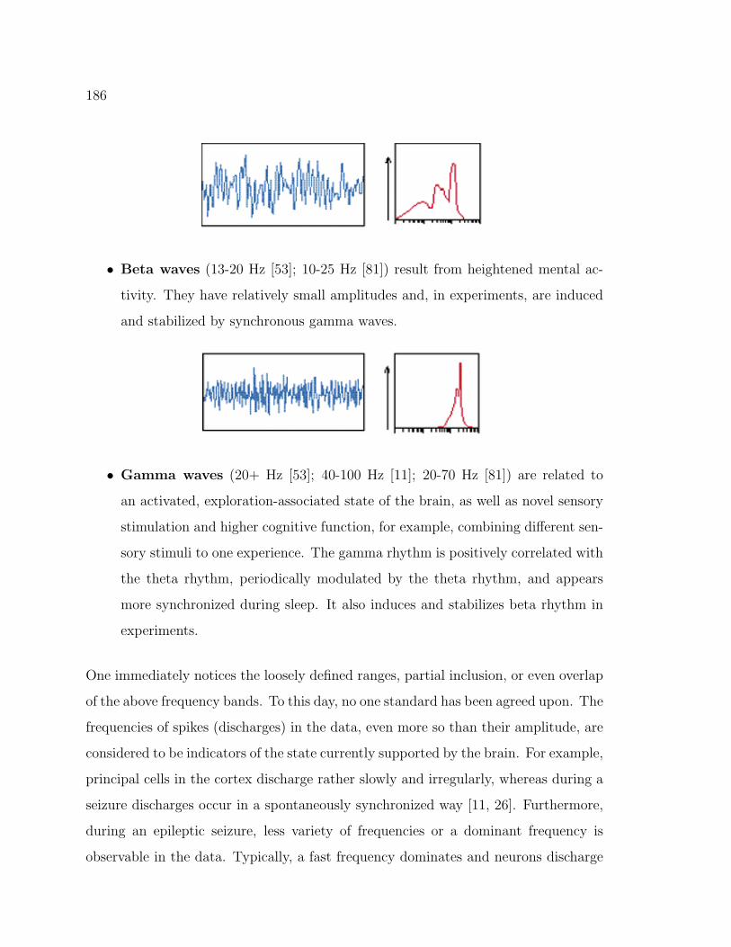
186
• Beta waves (13-20 Hz [53]; 10-25 Hz [81]) result from heightened mental ac-
tivity. They have relatively small amplitudes and, in experiments, are induced
and stabilized by synchronous gamma waves.
• Gamma waves (20+ Hz [53]; 40-100 Hz [11]; 20-70 Hz [81]) are related to
an activated, exploration-associated state of the brain, as well as novel sensory
stimulation and higher cognitive function, for example, combining different sen-
sory stimuli to one experience. The gamma rhythm is positively correlated with
the theta rhythm, periodically modulated by the theta rhythm, and appears
more synchronized during sleep. It also induces and stabilizes beta rhythm in
experiments.
One immediately notices the loosely defined ranges, partial inclusion, or even overlap
of the above frequency bands. To this day, no one standard has been agreed upon. The
frequencies of spikes (discharges) in the data, even more so than their amplitude, are
considered to be indicators of the state currently supported by the brain. For example,
principal cells in the cortex discharge rather slowly and irregularly, whereas during a
seizure discharges occur in a spontaneously synchronized way [11, 26]. Furthermore,
during an epileptic seizure, less variety of frequencies or a dominant frequency is
observable in the data. Typically, a fast frequency dominates and neurons discharge
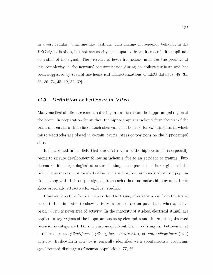
187
in a very regular, “machine like” fashion. This change of frequency behavior in the
EEG signal is often, but not necessarily, accompanied by an increase in its amplitude
or a shift of the signal. The presence of fewer frequencies indicates the presence of
less complexity in the neurons’ communication during an epileptic seizure and has
been suggested by several mathematical characterizations of EEG data [67, 48, 31,
33, 80, 74, 45, 12, 59, 32].
C.3 Definition of Epilepsy in Vitro
Many medical studies are conducted using brain slices from the hippocampal region of
the brain. In preparation for studies, the hippocampus is isolated from the rest of the
brain and cut into thin slices. Each slice can then be used for experiments, in which
micro electrodes are placed in certain, crucial areas or positions on the hippocampal
slice.
It is accepted in the field that the CA1 region of the hippocampus is especially
prone to seizure development following ischemia due to an accident or trauma. Fur-
thermore, its morphological structure is simple compared to other regions of the
brain. This makes it particularly easy to distinguish certain kinds of neuron popula-
tions, along with their output signals, from each other and makes hippocampal brain
slices especially attractive for epilepsy studies.
However, it is true for brain slices that the tissue, after separation from the brain,
needs to be stimulated to show activity in form of action potentials, whereas a live
brain in situ is never free of activity. In the majority of studies, electrical stimuli are
applied to key regions of the hippocampus using electrodes and the resulting observed
behavior is categorized. For our purposes, it is sufficient to distinguish between what
is referred to as epileptiform (epilepsy-like, seizure-like), or non-epileptiform (etc.)
activity. Epileptiform activity is generally identified with spontaneously occurring,
synchronized discharges of neuron populations [77, 26].
188
The two main purposes of cell-cell signaling are to cause excitatory or inhibitory
effects on the downstream target. One of the easiest ways to induce epileptiform
behavior in brain slices is to disable the inhibitory feedback control for certain types
of neurons, which then exhibit hyper-excited responses to given stimuli. However,
seizure-like behavior in brain slices can be induced in a variety of ways, only few
of which are linked to synaptic inhibition. In fact, it has been shown that hyper-
synchronous epileptiform activity can be dissociated from hyper-excited neural re-
sponses. In other words, spontaneous epileptiform activity can be maintained in
brain slices without interfering with the cells’ synaptic excitability. Instead, the al-
ternative pathway for seizure development lies in the direct interaction of cells at their
soma, mediated by gap-junctions and involving direct electrical field interactions [26].
This seems to suggest a more physical, rather than biological, basis for epileptiform
activity.
Even though different pathways to epileptiform behavior have been discovered in a
variety of preparations, the characteristics of seizure-like activity are very similar. In
other words, different initial causes lead to the same, common result. One might stip-
ulate that, for each of these cases, the chains of causal events eventually merge, such
that the events in the immediate vicinity of the common event (seizure) are roughly
the same. Hence, it has been suggested that the fundamental events leading to seizure
initiation and termination might also be similar [78]. However, since stimulation in
brain slices occurs artificially and communicative pathways are severely restricted, it
remains a question how closely the results obtained from brain slices can be related
to the behavior of cells which are still part of the connected tissue.
C.4 Relevant Knowledge About Epileptic Neuron
Looking at seizure disorders in particular, provides us with more criteria about what
processes might be important to include. Having studied the special conditions and
189
symptoms of epilepsy especially at the cellular level, we find the following points
particularly relevant:
The CA1 region of the hippocampus is especially prone to seizure development
following ischemia. Regional variation in cell density in the hippocampus has been
linked to this weakness [50], which implies that cell density or relative cell volume may
be key factors in seizure disorders. Further, it has been observed that neurons swell
during activity and extrude potassium to the extracellular space. Since the neurons
are active in a way often described as “machine-like” during epileptic seizures, one
can imagine that potassium extrusion happens to an extreme extent. This implies
that, in addition to cell volume, potassium may also be one of our key players. In
fact, numerous independent studies [6, 50, 68, 78, 26, 25] have shown that
1. Potassium concentration in the extracellular space increases more than 3-fold
during seizures (or seizure-like activity in brain slices). More precisely, a normal
extracellular level of K is about 3 mM, whereas during seizures levels of up to
10 mM can be reached.
2. Seizure-like activity is induced more easily in brain slices after having bathed
them in high potassium medium with concentrations comparable to those ob-
served during seizures. In other words, significantly less of a seizure triggering
substance is needed to induce seizure-like activity in high potassium medium.
3. Bathing neurons in high potassium media also induces significant swelling of
the cells. In particular, a 10% decrease in osmolarity of the extracellular space,
which is well within physiological range, lead to a 47% or 55% increase in volume
of pyramidal or inter-neuron cells, respectively.
4. Any seizure or seizure-like activity is terminated immediately when a diuretic
is applied to reduce the cell volume. This has been demonstrated in both brain
slices and living animals alike.
190
5. Treating neurons in the CA1 region of the hippocampus with low extracellular
chloride medium while they are showing seizure-like activity desynchronizes
their discharges within minutes, even if high K is present.
6. Blocking the gradient driven Na-K-Cl co-transporter that transports Cl into
and Na and K out of the cell, abolishes epileptiform activity in the CA1 region
of hippocampal slices by desynchronizing population discharges.
For all the above reasons, understanding the causal relationships between the cell
volume, extracellular K concentration, possibly extracellular Cl concentration, and
seizure-like activity would mean a big step toward improving the understanding of
epileptic seizures.
C.5 Nonlinear Dynamics and Epilepsy
Several studies in neuronal network modeling [75, 47, 13] and analysis of clinical
epileptic EEGs have pointed out a possible framework for understanding the inter-
mittency of epilepsy [3, 19, 31, 48] based on the recent development in the field of
nonlinear dynamics [37]. The most important implication of the idea is that the brain
is a dynamical system (e.g., neuronal activities changing with time) with nonlinearity.
It is known that a nonlinear system can exhibit several characteristically differ-
ent behaviors dependent on the initial state of the system and subtle differences in
its parameters. For a linear system, the dynamic behavior of two slightly different
initial conditions will keep being slightly different, that is “small causes lead to small
effects”. However, the presence of unpredictability in the deterministic but nonlinear
dynamical system causes initially neighboring states to diverge exponentially fast as
the system evolves forward in time. The Lyapunov exponent is a quantitative index
for characterizing this behavior. A deterministic equation can, in this sense, gener-
ate seemingly random data without any noise input. This is known as “chaos” [5].
191
A significant consequence of this view is that although EEG data can be seemingly
stochastic, it could possibly be characterized by a rather simple and deterministic
mathematical model.
There are many models of single neurons or neuron populations, their analytical
treatments, and, even more so, their numerical simulations. They help explain the
way neuron populations communicate, are made to fit experimental data, provide help
in understanding specific diseases on a cellular level by motivating new studies, and
possibly help in developing new treatments. One key question that remains regarding
the connection of dynamical systems to epilepsy is whether an episode is a temporary
detour from otherwise healthy brain dynamics, or whether it is an intermittently
reappearing symptom of unhealthy brain dynamics. This is an important distinction:
The first case implies that both, healthy and epileptic, brain dynamics are modeled
by the same dynamical system, whereas the second case implies that healthy brain
dynamics are modeled by a qualitatively different dynamical system from epileptic
dynamics.
192
Appendix D
INTEGRALS OF EQUILIBRIUM SOLUTIONS
Boltzmann’s law is valid at equilibrium and, for example, in the internal compart-
ment
ci (x) eziϕ(x) = cLi eziϕ(L). (D.1)
Thus, the exact expression describing the mass of species i in the internal compart-
ment is correctly formulated as
vincini = (vin − LAc) cL
i + Ac
∫ 0
LcLi e−zi(ϕ(x)−ϕ(L))dx (D.2)
and explicit expressions for the integrals of exp (−zi (ϕ (x)− ϕ (x0))) for x0 ∈ L, R
would be desirable to have at hand. We shall recall the equilibrium solutions derived
in section 2.3 for systems containing species carrying any of the valencies ±1 and ±2:
When the valency j = −2 is present in the system, we make use of the following
notation:
u1,2 =1
2α−2
[− (2α−2 + α−1)±
√(2α−2 + α−1)
2 − 4α−2α2
]≤ 0 (D.3)
b = (1− u1) + (1− u2) , and c = (1− u1) (1− u2) (D.4)
σ =
+√
2cα−2
εfor L < x < 0
−√
2cα−2
εfor 0 < x < R
(D.5)
193
L (u) =
u−1
2√
c(u−u1)(u−u2)+2c+b(u−1)for u1 6= u2
u−12c+b(u−1)
for u1 = u2
(D.6)
Λ (x) = L (u0) exp (σx) . (D.7)
In case u1 6= u2, the explicit equilibrium solution, u (x) = exp (ϕ (x)− ϕ (x0)) for
x0 ∈ L, R, can be written as:
u = 1 +4cΛ
(1− bΛ)2 − 4cΛ2, (D.8)
whereas in case u1 = u2, the explicit solution, u (x) = exp (ϕ (x)− ϕ (x0)) for x0 ∈
L, R, may be written as:
u = 1 +2cΛ
1− bΛ. (D.9)
When the valency j = −2 is not present in the system, we make use of the following
notation:
u2 =−α2
α1 + 2α2
≤ 0. (D.10)
σ =
+√
2(1−u2)α−1
εfor L < x < 0
−√
2(1−u2)α−1
εfor 0 < x < R
(D.11)
L (u) =
√u− u2 −
√1− u2√
u− u2 +√
1− u2
(D.12)
Λ (x) = L (u0) exp (σx) . (D.13)
The explicit solution, u (x) = exp (ϕ (x)− ϕ (x0)) for x0 ∈ L, R, may then be
written as:
u = u2 + (1− u2)(
1 + Λ
1− Λ
)2
. (D.14)
194
In the special case of only monovalent species (valencies ±1) in the system, u2 = 0
and solution (D.14) reduces to
u =(
1 + Λ
1− Λ
)2
. (D.15)
In order to describe the mass in either compartment or in the entire system, we derive
integrals of u−zi (x) = exp (−zi (ϕ (x)− ϕ (x0))) for x0 ∈ L, R and appropriate
valencies, zi. Since
dΛ = σΛ dx, (D.16)
a change of variables from x to Λ, such that∫
u dx = 1σ
∫u ·Λ−1dΛ, and decomposing
each solution into its partial fractions allows us to obtain expressions for the desired
integrals by simply computing and combining integrals of rational functions.
D.1 Integrals in case of a mono-valent system
Consider first the integral of u (x) = exp (ϕ (x)− ϕ (x0)) for x0 ∈ L, R. We shall
return later to computing the integral of u−1 (x) = exp (− (ϕ (x)− ϕ (x0))). Decom-
posing the solution to the mono-valent system yields
u =(
1 + Λ
1− Λ
)2
(D.17)
=1
(1− Λ)2 + 2Λ
(1− Λ)2 +Λ2
(1− Λ)2 (D.18)
and
uΛ−1 =1
Λ (1− Λ)2 +2
(1− Λ)2 +Λ
(1− Λ)2 (D.19)
=1
Λ+
4
(1− Λ)2 . (D.20)
The integrals, of which∫
u dx =∫
u · Λ−1dΛ is composed, are∫ 1
ΛdΛ = lnΛ (D.21)∫ 1
(1− Λ)2dΛ =1
1− Λ(D.22)
195
and so ∫ x2
x1
u dx =1
σ
[lnΛ +
4
1− Λ
]∣∣∣∣Λ(x2)
Λ(x1). (D.23)
To compute the integral of u−1 (x) = exp (− (ϕ (x)− ϕ (x0))), we decompose
u−1 =(
1− Λ
1 + Λ
)2
(D.24)
=1
(1 + Λ)2 − 2Λ
(1 + Λ)2 +Λ2
(1 + Λ)2 (D.25)
and
u−1Λ−1 =1
Λ (1 + Λ)2 −2
(1 + Λ)2 +Λ
(1 + Λ)2 (D.26)
=1
Λ− 4
(1 + Λ)2 . (D.27)
The integrals, of which∫
u−1 dx =∫
u−1 · Λ−1dΛ is composed, are∫ 1
ΛdΛ = lnΛ (D.28)∫ 1
(1 + Λ)2dΛ =−1
1 + Λ(D.29)
and so ∫ x2
x1
u−1dx =1
σ
[lnΛ +
4
1 + Λ
]∣∣∣∣Λ(x2)
Λ(x1). (D.30)
D.2 Integrals in case no valency j = −2 is present
Consider first the integral of u (x) = exp (ϕ (x)− ϕ (x0)) for x0 ∈ L, R. We shall
return later to computing the integrals of u−1 (x) = exp (− (ϕ (x)− ϕ (x0))) and
u2 (x) = exp (2 (ϕ (x)− ϕ (x0))). Note that, in case no valency of +2 is present,
the results of this section reduce to the results of section D.1. Decomposing the
solution yields
u = u2 + (1− u2)(
1 + Λ
1− Λ
)2
(D.31)
= u2 + (1− u2)
(1
(1− Λ)2 + 2Λ
(1− Λ)2 +Λ2
(1− Λ)2
), (D.32)
196
for which we may reuse the results of section D.1 and obtain∫ x2
x1
u dx =1
σ
[lnΛ + (1− u2)
4
1− Λ
]∣∣∣∣Λ(x2)
Λ(x1). (D.33)
Computing the integral of u−1 (x) = exp (− (ϕ (x)− ϕ (x0))) is not as trivial. Decom-
posing the inverse of u yields
u−1 =1
u2 + (1− u2)(
1+Λ1−Λ
)2 (D.34)
=(1− Λ)2
u2 (1− Λ)2 + (1− u2) (1 + Λ)2 (D.35)
=(1− Λ)2
(1 + Λ)2 − 4u2Λ(D.36)
=Λ2 − 2Λ + 1
Λ2 + (2− 4u2) Λ + 1(D.37)
and thus
u−1Λ−1 =1
Λ (Λ2 + (2− 4u2) Λ + 1)+
Λ2 − 2Λ
Λ2 + (2− 4u2) Λ + 1(D.38)
=1
Λ− (1− u2)
4
(Λ2 + (2− 4u2) Λ + 1). (D.39)
The quantity
∆ = 4− (2− 4u2)2 = 16u2 (1− u2) < 0 (D.40)
and thus the integrals, of which∫
u−1 dx =∫
u−1 · Λ−1dΛ is composed, are
∫ 1
ΛdΛ = lnΛ (D.41)
∫ dΛ
Λ2 + (2− 4u2) Λ + 1=
1
4√
(−u2) (1− u2)ln
Λ +(√−u2 −
√1− u2
)2
Λ +(√−u2 +
√1− u2
)2
.(D.42)
Finally,
∫ x2
x1
u−1dx =1
σ
lnΛ−√
1− u2
−u2
ln
Λ +(√−u2 −
√1− u2
)2
Λ +(√−u2 +
√1− u2
)2
∣∣∣∣∣∣∣Λ(x2)
Λ(x1)
. (D.43)
197
To compute the integral of u2 (x) = exp (− (ϕ (x)− ϕ (x0))), we decompose u2, that
is
u2 =
(u2 + (1− u2)
(1 + Λ
1− Λ
)2)2
(D.44)
=
(1 + (1− u2)
4Λ
(1− Λ)2
)2
(D.45)
= 1 + (1− u2)8Λ
(1− Λ)2 + (1− u2)2 16Λ2
(1− Λ)4 (D.46)
For the first two terms we can reuse results from section D.1, whereas for the third
term we need the integral
∫ Λ dΛ
(1− Λ)4 =−1
2 (1− Λ)2 +1
3 (1− Λ)3 . (D.47)
Combining results, we obtain the final integral needed in this case,∫ x2
x1
u2dx =1
σ
[lnΛ +
8 (1− u2)
(1− Λ)+−16 (1− u2)
2
2 (1− Λ)2 +16 (1− u2)
2
3 (1− Λ)3
]∣∣∣∣∣Λ(x2)
Λ(x1)
. (D.48)
D.3 Integrals in case valency j = −2 is present and u1 6= u2
Consider first the integral of u (x) = exp (ϕ (x)− ϕ (x0)) for x0 ∈ L, R. We shall
return later to computing the integrals of u−1 (x) = exp (− (ϕ (x)− ϕ (x0))), u2 (x) =
exp (2 (ϕ (x)− ϕ (x0))), and u−2 (x) = exp (−2 (ϕ (x)− ϕ (x0))). Decomposing the
solution yields
u = 1 +4cΛ
(1− bΛ)2 − 4cΛ2(D.49)
= 1 +4cΛ
(1− (4c + b) Λ) (1− (4c− b) Λ). (D.50)
The integrals we need to compute∫
u dx = 1σ
∫u · Λ−1dΛ are∫ 1
ΛdΛ = lnΛ (D.51)∫ dΛ
(1− (4c + b) Λ) (1− (4c− b) Λ)=
1
2bln
(1− (4c− b) Λ
1− (4c + b) Λ
)(D.52)

198
and thus, the integral of u in this case is
∫ x2
x1
u dx =1
σ
[lnΛ +
2c
bln
(1− (4c− b) Λ
1− (4c + b) Λ
)]∣∣∣∣∣Λ(x2)
Λ(x1)
. (D.53)
To obtain the integral of u−1, we rewrite
u−1 =1
1 + 4cΛ(1−bΛ)2−4cΛ2
(D.54)
=(1− bΛ)2 − 4cΛ2
(1− bΛ)2 − 4cΛ2 + 4cΛ(D.55)
= 1− 4cΛ
(b2 − 4c) Λ2 + 2 (2c− b) Λ + 1(D.56)
= 1− 4cΛ
(b2 − 4c) (Λ− Λ1) (Λ− Λ2), (D.57)
where
Λ1,2 =2 (2c− b)±
√−∆
2 (b2 − 4c)(D.58)
= −
(√(−u1) (1− u2)±
√(−u2) (1− u1)
)2
(u1 − u2)2 < 0 (D.59)
−∆ = 16u1u2 (1− u1) (1− u2) > 0 (D.60)
b2 − 4c = ((1− u1)− (1− u2))2 = (u1 − u2)
2 (D.61)
2c− b = (−u1) (1− u2) + (−u2) (1− u1) (D.62)
2 (2c− b)±√−∆ = 2
(√(−u1) (1− u2)±
√(−u2) (1− u1)
)2
. (D.63)
The integral needed to compute∫
u−1 dx =∫
u−1 · Λ−1dΛ is
∫ dΛ
(Λ− Λ1) (Λ− Λ2)=
1
Λ1 − Λ2
ln(
Λ− Λ1
Λ− Λ2
), (D.64)
so that ∫ x2
x1
u−1dx =1
σ
[lnΛ +
2c√−∆ (b2 − 4c)
ln(
Λ− Λ1
Λ− Λ2
)]∣∣∣∣∣Λ(x2)
Λ(x1)
. (D.65)
To compute the integrals of u2, we rewrite
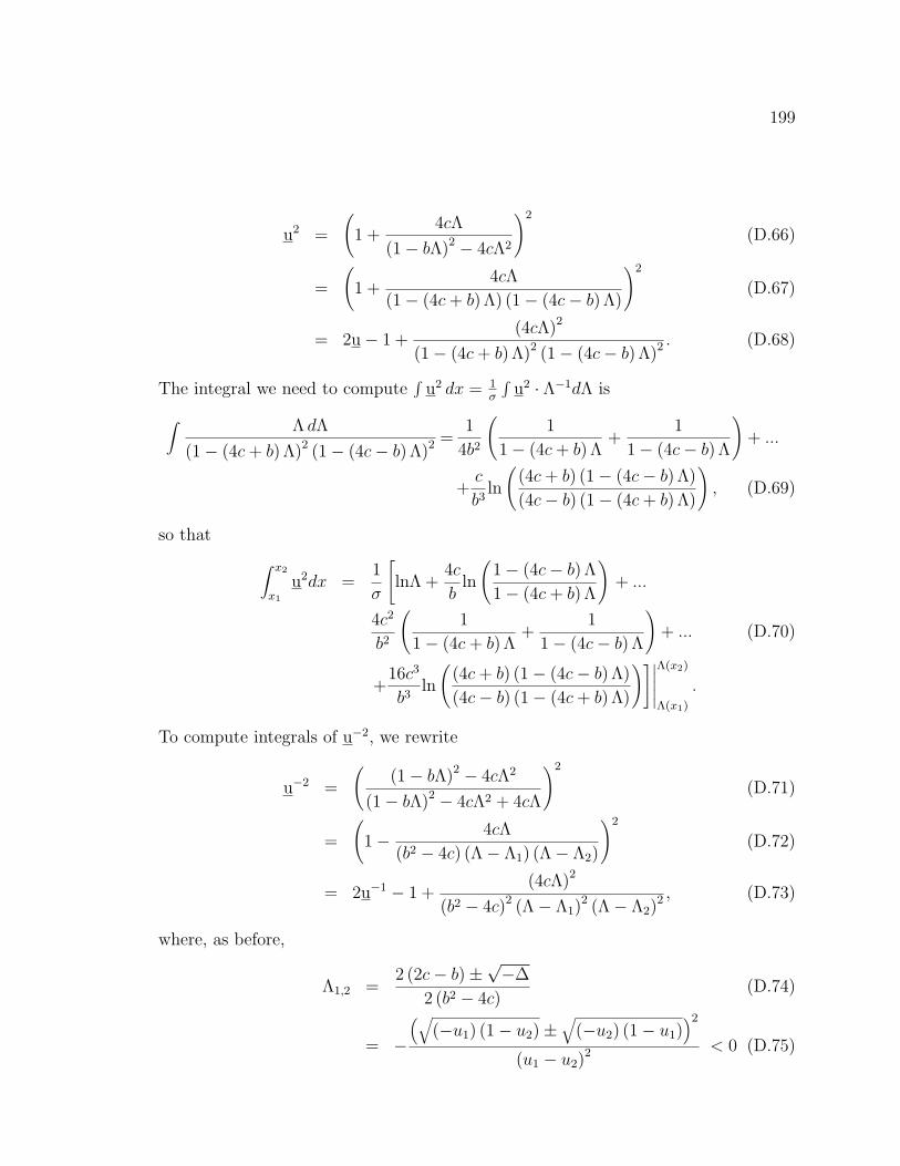
199
u2 =
(1 +
4cΛ
(1− bΛ)2 − 4cΛ2
)2
(D.66)
=
(1 +
4cΛ
(1− (4c + b) Λ) (1− (4c− b) Λ)
)2
(D.67)
= 2u− 1 +(4cΛ)2
(1− (4c + b) Λ)2 (1− (4c− b) Λ)2 . (D.68)
The integral we need to compute∫
u2 dx = 1σ
∫u2 · Λ−1dΛ is
∫ Λ dΛ
(1− (4c + b) Λ)2 (1− (4c− b) Λ)2 =1
4b2
(1
1− (4c + b) Λ+
1
1− (4c− b) Λ
)+ ...
+c
b3ln
((4c + b) (1− (4c− b) Λ)
(4c− b) (1− (4c + b) Λ)
), (D.69)
so that ∫ x2
x1
u2dx =1
σ
[lnΛ +
4c
bln
(1− (4c− b) Λ
1− (4c + b) Λ
)+ ...
4c2
b2
(1
1− (4c + b) Λ+
1
1− (4c− b) Λ
)+ ... (D.70)
+16c3
b3ln
((4c + b) (1− (4c− b) Λ)
(4c− b) (1− (4c + b) Λ)
)]∣∣∣∣∣Λ(x2)
Λ(x1)
.
To compute integrals of u−2, we rewrite
u−2 =
((1− bΛ)2 − 4cΛ2
(1− bΛ)2 − 4cΛ2 + 4cΛ
)2
(D.71)
=
(1− 4cΛ
(b2 − 4c) (Λ− Λ1) (Λ− Λ2)
)2
(D.72)
= 2u−1 − 1 +(4cΛ)2
(b2 − 4c)2 (Λ− Λ1)2 (Λ− Λ2)
2 , (D.73)
where, as before,
Λ1,2 =2 (2c− b)±
√−∆
2 (b2 − 4c)(D.74)
= −
(√(−u1) (1− u2)±
√(−u2) (1− u1)
)2
(u1 − u2)2 < 0 (D.75)

200
−∆ = 16u1u2 (1− u1) (1− u2) > 0 (D.76)
b2 − 4c = ((1− u1)− (1− u2))2 = (u1 − u2)
2 (D.77)
2c− b = (−u1) (1− u2) + (−u2) (1− u1) (D.78)
2 (2c− b)±√−∆ = 2
(√(−u1) (1− u2)±
√(−u2) (1− u1)
)2
. (D.79)
The integral we need to compute∫
u−2dx = 1σ
∫u−2 · Λ−1dΛ is
∫ Λ dΛ
(b2 − 4c)2 (Λ− Λ1)2 (Λ− Λ2)
2 =1
−∆
(−Λ1
(Λ− Λ1)+
−Λ2
(Λ− Λ2)
)+ ...
+(2c− b)√−∆
3 ln(
Λ− Λ1
Λ− Λ2
), (D.80)
so that
∫ x2
x1
u−2dx =1
σ
[lnΛ +
4c√−∆ (b2 − 4c)
ln(
Λ− Λ1
Λ− Λ2
)+ ... (D.81)
+16c2
−∆
(−Λ1
(Λ− Λ1)+
−Λ2
(Λ− Λ2)
)+ ... (D.82)
+16c2 (2c− b)√−∆
3 ln(
Λ− Λ1
Λ− Λ2
)]∣∣∣∣∣Λ(x2)
Λ(x1)
. (D.83)
201
VITA
Viktoria R.T. Krupp was born of Viktor A. and Gisela T. (Krause) Krupp in
Dusseldorf, Germany. After finishing Highschool with majors in Mathematics and
Chemistry, she took up studies in Technomathematik at the Gerhard Mercator Uni-
versitat-GH Duisburg from 1994 to 1997. A member of the prestigeous German
National Merit Scholarship Foundation (Studienstiftung des deutschen Volkes, e.V.)
from 1995 through 2000, she transferred to the University of Washington Graduate
School in 1997. In the Department of Applied Mathematics, she earned a Master of
Science in 1999, continued the study of Mathematical Biology with her advisor, Hong
Qian, and received the departmental Boeing Award of Excellence in 2002. After her
graduation with a Doctor of Philosophy in Applied Mathematics, Viktoria is excited
to continue and extend her work while holding a research position with Jim Keener
and Aaron Fogleson at the University of Utah.
Viktoria met her husband, Terry Hsu of Seattle, while Salsa dancing in 1998, they
were married in 2001, and Viktoria’s last name changed from Krupp to Hsu (spoken
“shoe”). To date, the most original comment about this name change has to be
accounted to Bard Ermentrout: At their first meeting, he pointed out that “this shoe
doesn’t fit.” Besides dancing, the couple enjoys music, cooking and eating good food,
their two cats, swimming, and a variety of outdoor activities.