ion multi-nose structures observed by cluster in the inner

HAL Id: hal-00330112https://hal.archives-ouvertes.fr/hal-00330112

Submitted on 1 Feb 2007

HAL is a multi-disciplinary open accessarchive for the deposit and dissemination of sci-entific research documents, whether they are pub-lished or not. The documents may come fromteaching and research institutions in France orabroad, or from public or private research centers.

L’archive ouverte pluridisciplinaire HAL, estdestinée au dépôt et à la diffusion de documentsscientifiques de niveau recherche, publiés ou non,émanant des établissements d’enseignement et derecherche français ou étrangers, des laboratoirespublics ou privés.

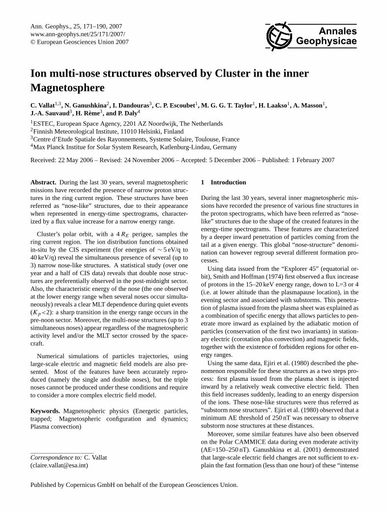
Ion multi-nose structures observed by Cluster in theinner Magnetosphere

C. Vallat, N. Ganushkina, I. Dandouras, C. P. Escoubet, M. G. G. T. Taylor,H. Laakso, A. Masson, J.-A. Sauvaud, H. Rème, P. Daly

To cite this version:C. Vallat, N. Ganushkina, I. Dandouras, C. P. Escoubet, M. G. G. T. Taylor, et al.. Ion multi-nose structures observed by Cluster in the inner Magnetosphere. Annales Geophysicae, EuropeanGeosciences Union, 2007, 25 (1), pp.171-190. <hal-00330112>

https://hal.archives-ouvertes.fr/hal-00330112

https://hal.archives-ouvertes.fr

Ann. Geophys., 25, 171–190, 2007www.ann-geophys.net/25/171/2007/© European Geosciences Union 2007

AnnalesGeophysicae

Ion multi-nose structures observed by Cluster in the innerMagnetosphere

C. Vallat1,3, N. Ganushkina2, I. Dandouras3, C. P. Escoubet1, M. G. G. T. Taylor 1, H. Laakso1, A. Masson1,J.-A. Sauvaud3, H. Reme3, and P. Daly4

1ESTEC, European Space Agency, 2201 AZ Noordwijk, The Netherlands2Finnish Meteorological Institute, 11010 Helsinki, Finland3Centre d’Etude Spatiale des Rayonnements, Systeme Solaire, Toulouse, France4Max Planck Institue for Solar System Research, Katlenburg-Lindau, Germany

Received: 22 May 2006 – Revised: 24 November 2006 – Accepted: 5 December 2006 – Published: 1 February 2007

Abstract. During the last 30 years, several magnetosphericmissions have recorded the presence of narrow proton struc-tures in the ring current region. These structures have beenreferred as “nose-like” structures, due to their appearancewhen represented in energy-time spectrograms, character-ized by a flux value increase for a narrow energy range.

Cluster’s polar orbit, with a 4RE perigee, samples thering current region. The ion distribution functions obtainedin-situ by the CIS experiment (for energies of∼ 5 eV/q to40 keV/q) reveal the simultaneous presence of several (up to3) narrow nose-like structures. A statistical study (over oneyear and a half of CIS data) reveals that double nose struc-tures are preferentially observed in the post-midnight sector.Also, the characteristic energy of the nose (the one observedat the lower energy range when several noses occur simulta-neously) reveals a clear MLT dependence during quiet events(Kp<2): a sharp transition in the energy range occurs in thepre-noon sector. Moreover, the multi-nose structures (up to 3simultaneous noses) appear regardless of the magnetosphericactivity level and/or the MLT sector crossed by the space-craft.

Numerical simulations of particles trajectories, usinglarge-scale electric and magnetic field models are also pre-sented. Most of the features have been accurately repro-duced (namely the single and double noses), but the triplenoses cannot be produced under these conditions and requireto consider a more complex electric field model.

Keywords. Magnetospheric physics (Energetic particles,trapped; Magnetospheric configuration and dynamics;Plasma convection)

Correspondence to:C. Vallat([email protected])

1 Introduction

During the last 30 years, several inner magnetospheric mis-sions have recorded the presence of various fine structures inthe proton spectrograms, which have been referred as “nose-like” structures due to the shape of the created features in theenergy-time spectrograms. These features are characterizedby a deeper inward penetration of particles coming from thetail at a given energy. This global “nose-structure” denomi-nation can however regroup several different formation pro-cesses.

Using data issued from the “Explorer 45” (equatorial or-bit), Smith and Hoffman (1974) first observed a flux increaseof protons in the 15–20 keV energy range, down to L=3 or 4(i.e. at lower altitude than the plasmapause location), in theevening sector and associated with substorms. This penetra-tion of plasma issued from the plasma sheet was explained asa combination of specific energy that allows particles to pen-etrate more inward as explained by the adiabatic motion ofparticles (conservation of the first two invariants) in station-ary electric (corotation plus convection) and magnetic fields,together with the existence of forbidden regions for other en-ergy ranges.

Using the same data, Ejiri et al. (1980) described the phe-nomenon responsible for these structures as a two steps pro-cess: first plasma issued from the plasma sheet is injectedinward by a relatively weak convective electric field. Thenthis field increases suddenly, leading to an energy dispersionof the ions. These nose-like structures were thus referred as“substorm nose structures”. Ejiri et al. (1980) observed that aminimum AE threshold of 250 nT was necessary to observesubstorm nose structures at these distances.

Moreover, some similar features have also been observedon the Polar CAMMICE data during even moderate activity(AE=150–250 nT). Ganushkina et al. (2001) demonstratedthat large-scale electric field changes are not sufficient to ex-plain the fast formation (less than one hour) of these “intense

Published by Copernicus GmbH on behalf of the European Geosciences Union.

172 C. Vallat et al.: Ion multi-nose structures

nose events”, as named by the authors. They showed that lo-cal pulses in the electric field (up to 4 mV/m) associated withsubstorm dipolarization are necessary to explain such rapidformation time and radial location of the observed features.

Some nose-shaped structures were observed by Akebonoat altitudes up to 10 000 km. Shirai et al. (1997) interpretedthem in terms of mono-energetic ion drop off. These gaps,which appear at about 10 keV, were observed over a wide lati-tudinal range at almost constant energy. This gap comes usu-ally together with a simultaneous gap at lower energy, driv-ing to the creation of another type of nose-like structure, usu-ally at lower energy ranges than the substorm nose structures(i.e. below 10 keV). Moreover, these structures (that will bereferred in the following as “stationary nose structures”) ap-pear regardless of the magnetospheric activity level. Usingan ion drift trajectory model, Shirai et al. (1997) were able toreproduce such structures, and showed that they are the con-sequence of the open/close character of the particle orbits:at the Akebono location, corotation electric field is sufficientto close the orbit (around the Earth) of low energy particleswhich are drifting eastward. Also, the magnetic field gradientis strong enough to close the orbits of high energy particleswhich are drifting westward. As a consequence, for these en-ergies, particles are not continuously supplied from the tailregion. However, particles with intermediate energies are onopen orbits (neither corotational field nor magnetic field gra-dient permit to close their orbits around the Earth), creatingthe nose structures observed on the Akebono data.

Earlier on, Lennartsson et al. (1979), by analyzing ISEE-1data, demonstrated that in the morning sector the ion velocitydistribution was presenting a hole for a given energy range.This hole was explained in terms of the very long time ofresidence of particles with a given energy, for which the elec-tric field action (leading to an eastward drift of protons) andthe magnetic field action (leading to a westward drift of pro-tons) are antagonistic and almost compensate each other. Thedrastically decreased drift velocity of this population createsa spectral gap in some sectors of the magnetosphere, knownalso as “stagnation dip”.

More recently, Kovrazhkin et al. (1999) listed the differ-ent types of gaps observed on the ION spectrograms on-board the INTERBALL spacecraft: the one described byShirai et al. (1997) on Akebono data and the one describedby Lennartsson et al. (1979), corresponding to the very longtime of azimuthal drift of particles for a given energy.

Double nose structures (referred in the following as “splitnose”), as seen in the morning sector by the ION exper-iment onboard Interball-2, were studied by Buzulukova etal. (2003). They are interpreted by the authors as the resultof a superposition in the spectrograms of a single stationarynose (Shirai et al., 1997) together with the gap described andanalyzed by Lennartsson et al. (1979). This gap, which wasobserved in the morning and pre-morning sector, is createdat energies within the nose energy range, leading to a split ofthe stationary nose into two parts.

Polar also recorded multi bands (more than 2) of ions. Thisled to several interpretations: on one hand Li et al. (2000)explained it as the result of ion drift echoes following an in-crease of the convection electric field. Particles are injecteddeeply inward, following the electric field increase, and theystart to disperse, high energy particles drifting faster aroundthe Earth than low energy ones, their population superpos-ing the slower one locally. On the other hand, Ebihara etal. (2004) interpreted this feature as the result of two com-bined processes: a change in the convection electric field to-gether with a change in the distribution function of the sourceto explain the low energy particles features. They showedthat a change in the convection electric field can move thenose energy range to higher or lower energies, leading to thesimultaneous observation of the “old” nose (created beforethe convection electric field change) together with a new one.

This variety of structures, presenting roughly the same sig-natures on the energy-time spectrograms issued from severalmissions, are thus thought to have different origins and toappear at restricted locations and under specific activity con-ditions. Their frequency of appearance is however still underquestion, as well as the dominant mechanisms involved intheir formation.

Recent data obtained onboard the Cluster spacecraft by theCODIF/CIS ion mass spectrometers reveal also the presenceof different types of nose structures, for any MLT sector ormagnetospheric activity level. Here we present a statisti-cal study based on about 163 perigee passes of the Clusterspacecraft, aiming to extract the main characteristics of thesefeatures and to determine where they appear preferentially.Then, using numerical modeling, we try to understand themain process(es) responsible for the creation of such struc-tures, and what are the most influent parameters on the struc-ture’s shape. After a brief reminder concerning the Clustermission and its onboard plasma experiments (Sect. 2), wepresent CIS observations of single and multi-nose structuresobserved at different MLT locations (Sect. 3). Then, basedon more than one year and a half of data, a statistical studyover 163 Cluster perigee passes is presented (Sect. 4). Fi-nally, particle trajectory tracing is performed to understandthe main mechanisms involved in the structures formation,and the influence of magnetic and large scale electric fieldschanges on the structures observed (Sect. 5).

2 Instrumentation

2.1 Cluster

The Cluster mission is composed of four spacecraft launchedon closely spaced elliptical polar orbits, with a perigee atabout 4RE and apogee at about 19.6RE (Escoubet et al.,2001). This allows Cluster to cross the ring current regionfrom South to North during every perigee pass, and to ob-tain its latitudinal profile (Vallat et al., 2005). Moreover, due

Ann. Geophys., 25, 171–190, 2007 www.ann-geophys.net/25/171/2007/

C. Vallat et al.: Ion multi-nose structures 173

to the annual precession of its orbit, Cluster is crossing theequator at all MLT ranges over a year, allowing an equatorialpicture of the ring current at the Cluster’s perigee distance.

2.2 CIS

The Cluster Ion Spectrometry (CIS) experiment on boardCluster, which consists of the two complementary spec-trometers HIA and CODIF, provides the three-dimensionalion distributions with one spacecraft spin (4 s) time resolu-tion (Reme et al., 2001). The mass-resolving spectrometerCODIF provides the ionic composition of the plasma for themajor magnetospheric species (H+, He+, He++ and O+),from the thermal energy to about∼40 keV/e, covering thusa large part of the ring current energy range (Williams et al.,1987). HIA does not offer mass discrimination but has a bet-ter angular resolution (∼5.6◦) that is adequate for ion beamand solar wind measurements.

2.3 RAPID

At higher energies, the RAPID spectrometer (Research withAdaptive Particle Imaging Detectors) permits the detectionof suprathermal plasma distributions of electrons (from∼20to ∼400 keV) and ions (∼30 keV/nucleon to∼1500 keV)(Wilken et al., 2001). As a consequence, Cluster is capa-ble of sampling the entire ring current energy range duringits perigee pass (Williams et al., 1987).

3 Cluster observations

3.1 22 February 2002: single nose

During the 22 February 2002 perigee pass, Cluster is com-ing from the Southern lobe through the plasma sheet into thering current region. TheDst index of−6 nT reveals a verylow ring current activity during the Cluster equatorial cross-ing, at∼00:00 MLT. The AE index remains between 100 nTand 250 nT during the 10 h prior to the event. Cluster SC4data are presented in Fig. 1. This figure represents, fromtop to bottom: the RAPID proton flux (between 27.6 and1107 keV, with a data gap occurring just before the perigeepass), the proton spectrogram in particle flux units as mea-sured by CODIF, the pitch angle distribution of protons forthe∼0 to 10 keV energy range, the O+ spectrogram in fluxunits and the O+ pitch angle distribution for the∼0 to 10 keVenergy range. L-shells values, radial distance and invariantlatitudes are shown at the bottom of the figure. The red ar-row indicates the equatorial crossing.

Arriving from the Southern lobe, Cluster 4 encountersa boundary at 14:28 UT, characterizing its entry into thenear Earth plasma sheet. The proton population observedby CODIF has an isotropic distribution function. How-ever, at 14:50 UT, once Cluster arrives at lower latitudes

(|Ilat|=68.9◦, Southern hemisphere), a field aligned popula-tion appears, characterizing ion beams up-flowing from theionosphere and remaining until 14:58 UT (|Ilat|=67.4◦).

After 14:50 UT, RAPID is observing the smooth entranceof the spacecraft in the ring current, starting from lower en-ergy particles (around 30 keV) and extending up at all energyranges from 14:58 UT. Please note that for this event RAPIDdata were no longer available when approaching the equator.

After 15:30 UT, an ion gap is present from 19 keV andabove in the CODIF spectrogram, which extends to the lowerenergies with decreasing latitude of the spacecraft. This gappersists down to the equatorial plane both in the Southernand Northern hemispheres. A gap at lower energy ranges(from thermal energies up to 5.5 keV) appears abruptly at15:39 UT (|Ilat|=61.6◦). These two simultaneous gaps resultin the nose structure in the CODIF spectrogram, whose en-ergy is situated between 5.7 and 7.2 keV. The gap is also vis-ible by RAPID, characterized by a decrease in the flux in the27–68 keV channel as the spacecraft approaches the equato-rial plane. After the traversal of the equatorial plane in theNorthern hemisphere, the nose structure is still observed.

The main boundaries (i.e. lobe/near Earth plasma sheetand near Earth plasma sheet/ring current) are also observedin the O+ spectrograms. Moreover, up-flowing ions issuedfrom the ionosphere are seen in the spectrograms (14:50 to14:58 UT,|Ilat| between 68.9◦ and 67.4◦, respectively) andpresent an inverted “V” structure. Once inside the Plasmas-phere region (deduced from the CODIF-RPA data, see Sect. 7and Fig. 13), a nose structure is also observed for O+, withan energy range between 5.7 and 9.5 keV. Unfortunately, thereduced energy resolution of the O+ data does not allow us tounambiguously determine if both populations (O+ and H+)

present the nose structure at exactly the same energy. How-ever, both spectrograms (H+ and O+) have a similar appear-ance.

3.2 21 November 2001: “double” nose

The 21 November 2001 perigee pass occurs in the morningsector (MLT∼07:00), and reveals a somehow different fea-ture than the 22 February 2002 one. TheDst index of−12 nTcharacterizes the low activity level of the ring current, but theAE index reveals some substorm activity previous to the pass(4 to 14 h before, not shown). Cluster data are presented inFig. 2. Approaching from the Southern lobe, Cluster crossesthe dayside boundary layer at 19:09 UT (MLT∼8.5). Thisregion is characterized by a relatively isotropic distributionof ions (seen from∼19:30 UT) with energies of a few keVto a few tens of keV, and a density<5 cm−3.

At about 20:30 UT,|Ilat|=72◦, the spacecraft enter thering current region, signified by the appearance of trapped(α∼90◦)>10 keV ions. We note that the trapped populationis not obvious in the pitch angle plot of Fig. 2 due to thebroad energy range. By examining the RAPID proton data,we note that the low energy part of the ring current appears

www.ann-geophys.net/25/171/2007/ Ann. Geophys., 25, 171–190, 2007


Inv. Lat. 75.3 67.7 61.6 64.7 72.3

0-1

0 k

eV

0-1

0 k

eV

9

7

5

3

Fig. 1. SC4 particles data for the 22 February 2002 event. From top to bottom: RAPID proton flux in flux units, CIS/CODIF proton fluxin flux units, the proton pitch angle distribution in flux units for the 0–10 keV energy range, the O+ flux in flux unit, the O+ pitch angledistribution in flux unit for the 0 to 10 keV energy range and the L-shell values crossed by the spacecraft. Radial distance inRE and invariantlatitudes are indicated at the bottom of the plot. Red arrow indicated the equator crossing.

first, followed by an increase of the fluxes at higher energyranges as Cluster crosses lower L-shells. Near the Equa-tor, the maximum of the flux is observed within the 95.4 to168.7 keV energy channel of the RAPID instrument. SinceWilliams et al. (1987) stated that 90% of the ring current iscarried by particles with energy from 15 to 250 keV, this fluxmaximum is characteristic of this population. It is also worthnoting that, along the Cluster path and for the overall ringcurrent energy range (from 10 keV to 500 keV), lower en-ergy particle fluxes peak at higher L-shells. This has alreadybeen observed by AMPTE/CCE/CHEM at all MLT sectorsand for energies above 20 keV (Milillo et al., 2001).

At lower energies (i.e. below 10 keV), several popu-lations seem to emerge: on the one hand, down to|Ilat|=63◦ (21:17 UT, Southern Hemisphere) and|Ilat|=60.5◦

(22:17 UT, Northern Hemisphere), very narrow structures areseen at low energies (up to 1 keV), presenting a butterfly pitchangle distribution (not shown).

On the other hand, a trapped population co-exists atmedium energies (between 1.5 and 7 keV), which forms anose-like structure at low L-shells, centered around 3.8 keVand stationary between the inbound and the outbound ofthe Cluster orbit. Above this energy, another stationarynose-like structure appears around 16 keV, extending downto |Ilat|=62.6◦ (21:18 UT). These two noses co-exist locally.However, the equatorial edge of the lower energy nose is sit-uated at lower latitudes.

The gap separating the two noses persists throughoutthe perigee pass, from|Ilat|=69.9◦ in the Southern Hemi-sphere (20:40 UT) to|Ilat|=70.4◦ in the Northern Hemi-sphere (23:13 UT), its characteristic energy increasing withdecreasing latitude.

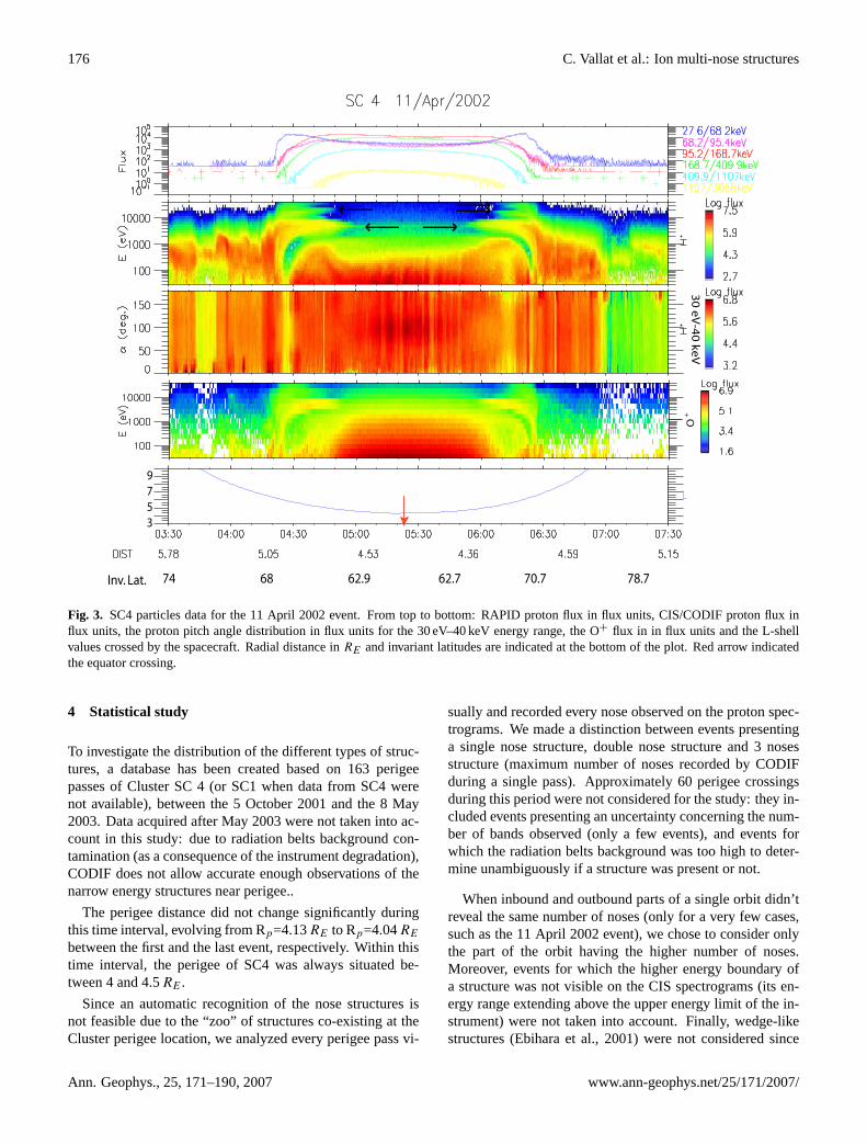
3.3 11 April 2002: “triple” nose

Multi noses structures are also evident in the CODIF spectro-grams during several Cluster perigee passes. Data for the 11April 2002 perigee pass (MLT∼21:00) are shown in Fig. 3.



Inv. lat. 84.7 77.7 66.4 60.5 69 80

30

eV

-40

ke

V

9

7

5

3

Fig. 2. SC4 particles data for the 21 November 2001 event. From top to bottom: RAPID proton flux in flux units, CIS/CODIF proton flux influx units, the proton pitch angle distribution in flux units for the 30 eV–40 keV energy range and the L-shell values crossed by the spacecraft.Radial distance inRE and invariant latitudes are indicated at the bottom of the plot. Red arrow indicated the equator crossing.

This event also takes place during a very quiet period, witha positiveDst index during more than two days precedingthe equatorial crossing by the spacecraft (Dst=21 nT duringthe crossing). TheKp index, always below 2 during the 12 hprior to this event, confirms these quiet magnetosphere con-ditions.

Initially in the magnetosheath, Cluster crosses the bound-ary layer before entering the ring current region at about04:14 UT (|Ilat|=67.2◦, Southern Hemisphere).

At energies higher than 3 keV, several nose structures areobserved simultaneously: at least two during the inboundpart of the orbit and three during the outbound (shown bythe black arrows).

The poleward edges of the two inbound noses start at|Ilat|=66.4◦ (Southern hemisphere, 04:21 UT), with thelower energy nose penetrating deeper (Lmin=4.63 for the nosecentered around 5 keV and Lmin=4.9 for the one centeredaround 18 keV). During the outbound part of the orbit, athird nose structure is detected at even higher energy (about26 keV), albeit with a dispersion looking smaller than the

other noses (however at those latitudes, this corresponds toa dispersion between Lmin=5.64 and Lmax=6.22).

In spite of a higher level of background in the O+ spectro-grams in the radiation belts (due to the longer time of flightof the O+ in the detection system), the first nose structure(characteristic energy below 10 keV) is also seen in the oxy-gen data. A second nose is present at higher energy duringthe inbound (between 15 and 20 keV) but no other nose isdetected for this population. However, since the energy dis-crimination is not as good for oxygen as for protons (16 en-ergy steps for O+, 31 for H+), it is possible that such narrowenergy structures are not resolved in the O+.

These three events, in spite of the similar activity of themagnetosphere and the same radial location of the spacecraft,are presenting strongly different features, i.e. single, doubleor triple nose structures.



Inv. Lat. 74 68 62.9 62.7 70.7 78.7

30

eV

-40

ke

V

9

7

5

3

O+

Fig. 3. SC4 particles data for the 11 April 2002 event. From top to bottom: RAPID proton flux in flux units, CIS/CODIF proton flux influx units, the proton pitch angle distribution in flux units for the 30 eV–40 keV energy range, the O+ flux in in flux units and the L-shellvalues crossed by the spacecraft. Radial distance inRE and invariant latitudes are indicated at the bottom of the plot. Red arrow indicatedthe equator crossing.

4 Statistical study

To investigate the distribution of the different types of struc-tures, a database has been created based on 163 perigeepasses of Cluster SC 4 (or SC1 when data from SC4 werenot available), between the 5 October 2001 and the 8 May2003. Data acquired after May 2003 were not taken into ac-count in this study: due to radiation belts background con-tamination (as a consequence of the instrument degradation),CODIF does not allow accurate enough observations of thenarrow energy structures near perigee..

The perigee distance did not change significantly duringthis time interval, evolving from Rp=4.13RE to Rp=4.04RE

between the first and the last event, respectively. Within thistime interval, the perigee of SC4 was always situated be-tween 4 and 4.5RE .

Since an automatic recognition of the nose structures isnot feasible due to the “zoo” of structures co-existing at theCluster perigee location, we analyzed every perigee pass vi-

sually and recorded every nose observed on the proton spec-trograms. We made a distinction between events presentinga single nose structure, double nose structure and 3 nosesstructure (maximum number of noses recorded by CODIFduring a single pass). Approximately 60 perigee crossingsduring this period were not considered for the study: they in-cluded events presenting an uncertainty concerning the num-ber of bands observed (only a few events), and events forwhich the radiation belts background was too high to deter-mine unambiguously if a structure was present or not.

When inbound and outbound parts of a single orbit didn’treveal the same number of noses (only for a very few cases,such as the 11 April 2002 event), we chose to consider onlythe part of the orbit having the higher number of noses.Moreover, events for which the higher energy boundary ofa structure was not visible on the CIS spectrograms (its en-ergy range extending above the upper energy limit of the in-strument) were not taken into account. Finally, wedge-likestructures (Ebihara et al., 2001) were not considered since



their characteristic energy, together with the structure theyare forming on the spectrograms, is somehow different fromthe nose ones (see Yamauchi et al., 2006).

For each of the 163 events the number of noses, their char-acteristic energy and the MLT sector crossed by the space-craft has been noted. Moreover, theKp andDst indices as-sociated to each event have also been listed. Over the 163perigee passes listed, 49 were not revealing any nose struc-ture, 71 were presenting a single nose structure, 40 were pre-senting a double nose structure and only 3 events revealedthree simultaneous noses.

4.1 Normalized occurrence of the numbers of simultaneousstructures (0, 1, 2 and 3) for various (Kp, MLT) couples

Figure 4 presents the normalized occurrence of the number ofenergy structures perKp index range. A distinction has beenmade between events presenting no nose structure (yellow),one nose (cyan), two noses (purple) or three noses structures(red).

Without further analysis, it already appears that for highactivity levels, the lack of nose seem to be the most fre-quent case. This can be understood since during high activityperiods (several successive substorms for example) freshlyinjected particles can hide the previously formed stationarynose structures.

During low and moderate activity periods, single nosestructures appear preferentially, but double nose is also of-ten observed.

Figure 5 presents the normalized occurrence of the num-ber of energy structures perKp index range, separatelyfor each of the four quadrants of the Magnetosphere (fromMLT=00:00 to 06:00, from MLT=06:00 to 12:00, fromMLT=12:00 to 18:00 and from MLT=18:00 to 00:00). Thenormalization is made over the number of passes per quad-rant and perKp range.

These plots reveal the overall changing distribution of thenumber of noses observed in the CODIF spectrograms withrespect to the MLT sector crossed by the spacecraft. Duringlow activity periods, double noses structures seem to occurfrequently, especially in the post-midnight and morning sec-tors.

Events for which CODIF recorded 3 noses remain excep-tional and no statistics can be made concerning this type offeature.

Concerning high activity events (Kp>4), zero and sin-gle nose structures are predominant. Nevertheless, the poorstatistics available for this kind of event is especially bad inthe 06:00–12:00 and 12:00–18:00 MLT sectors (dayside). Asa consequence, no conclusion can be made per MLT sector.

4.2 Characteristic energy of the nose vs. MLT

Figure 6 shows the mean energy of the nose structure (atits equatorial edge) for each of the 163 perigee passes, as

All MLT:

Normalized occurence of structure per Kp

0

10

20

30

40

50

60

0-1 2-3 4-6

Kp range

%

no nose

1 nose

2 noses

3 noses

Fig. 4. Normalized occurrence of the number of structures perKp

values.

a function of the MLT sector crossed by Cluster. When sev-eral nose structures occur simultaneously, the associated en-ergies are plotted, i.e. colored marks are used to distinguishthe lowest energy range nose (blue marks), the second one(pink squares) and the third one (yellow triangles) observedby CODIF. Some inaccuracies on the energy determinationcan occur since the energy resolution of the instrument is av-eraged over the mean energy of each energy bin.

Some remarks emerge:

This is the first time that multi-nose structures are ob-served over such a wide MLT range. Moreover, threesimultaneous noses are also observed occasionally in theevening sector (the few events presenting such structures aresituated in the 21:00–04:00 MLT sector).

In this plot (all activity levels included), we do not seeany clear relationship between the nose energy and the MLTsector where they are observed. However, if we make a dis-tinction between quiet events (i.e. withKp index up to 1) anddisturbed ones, we get the results shown in Figs. 7 and 8.

Even if the statistics are much more reduced, this quietevent selection (Fig. 7) presents a clearer trend of the energy-MLT dependence:

Focusing on the energy range of the first nose-like struc-ture (blue marks), we clearly observe an MLT dependenceof this characteristic energy range with the nose energy de-creasing from∼15 keV down to∼1 keV, counterclockwisefrom the pre noon sector (around MLT∼10:00).

Using a linear fit for the lower energy noses (see Fig. 7),we can deduce a relation between the energy of the nose andthe MLT sector:

E(keV) = −0.3276× MLT10 + 14.975 (1a)

and MLT10=MLT in hours in the dusk half sector (fromMLT=10 to MLT=24), and MLT10=MLT+24 otherwise. Thecorrelation coefficient is, in that case,r2=0.6339. A similartrend is also seen in the pink marks, representing the energyrange of the higher energy nose (when observed).



(a)

MLT= 12-18: Normalized occurence of structures

per Kp

0

20

40

60

80

100

120

0-1 2-3 4-6

Kp range

%

no nose

1 nose

2 noses

(c)

MLT=18-24: Normalized occurence of structures

per Kp

0

10

20

30

40

50

60

70

80

90

0-1 2-3 4-6

Kp range

%

no nose

1 nose

2 noses

3 noses

(b)

MLT=6-12: Normalized occurence of structures

per Kp

0

10

20

30

40

50

60

70

0-1 2-3 4-6

Kp range

%

no nose

1 nose

2 noses

(d)

MLT=0 to 6:

Normalized occurence of structures per Kp

0

10

20

30

40

50

60

70

0-1 2-3 4-6

Kp range

%

no nose

1 nose

2 noses

3 noses

Fig. 5. Normalized occurrence of structure type per (MLT,Kp) couples:(a) Upper left: MLT=12:00 to 18:00(b) Lower left: MLT=18:00 to 00:00(c) Upper right: MLT=06:00 to 12:00(d) Lower right: MLT=00:00 to 06:00

all Kp

0

5

10

15

20

25

30

35

10 13 16 19 22 01 04 07 10

MLT

En

erg

y (

keV

)

1st

2d

3d

Fig. 6. Characteristic energy of each nose-like structure observed byCODIF, as a function of the MLT sector crossed by Cluster. Bluemarks represent, when occurring, the nose observed at the lowerenergy range, whereas pink marks (resp. yellow) represent charac-teristic energies of the second (resp. third) nose-like structure.

Another way to show the data is to plot log (ENOSE) withrespect to MLT10, with ENOSE in eV :

log(ENOSE) = −0.0228× MLT10 + 4.3552 (1b)

Quiet periods Kp<2

0

5

10

15

20

25

30

35

10 13 16 19 22 01 04 07 10

MLT

En

erg

y (

keV

)

1st

2d

3d

Fig. 7. Characteristic energy of each nose structure vs. MLT, forKp=0 and 1.

with r2=0.5678 (plot not shown). However, during more ac-tive events (i.e.Kp=2 or 3, see Fig. 8), we do not observea trend for the lower energy nose as clear as for more quietevents (see Fig. 7). Even if the same global trend seems to bepresent, secondary trends are observed locally, especially inthe evening (21:00-00:00) and morning (06:00–12:00) sec-tors (see Fig. 8).



2<Kp<4

0

5

10

15

20

25

30

35

10 13 16 19 22 01 04 07 10

MLT

En

erg

y (

ke

V)

1st

2d

3d

Fig. 8. Characteristic energy of each nose structure vs. MLT, forKp=2 and 3.

In the morning sector, two trends appear for the lowestenergy nose: characteristic energy of the nose is found below5 keV for some events, whereas high energy is also foundin that sector, above 15 keV. This energy transition occursroughly in the same MLT sector that the one observed duringquiet events (Fig. 7), but this transition seems to occur over awider MLT range, i.e. from MLT∼05:00 to MLT∼09:00.

We also note the lack of double nose structures in thestatistics for the 21:00 to 01:00 MLT sector. However, char-acteristic energies vary a lot from one event to the other,reaching values from 5 keV up to 22 keV.

4.3 Characteristic energies of the lowest energy nose (foreach perigee pass), as a function of MLT andKp

Figure 9 shows the energy range of the nose as a function ofMLT and Kp. For events presenting a multi-nose structure,only the lowest energy nose has been considered.

Figure 9 reveals that, even if no linear relationship existsbetween the nose energy and theKp index, high energy nosestructures (i.e. above 15 keV) are only observed during dis-turbed periods (Kp>2). The variability of the nose energy isparticularly clear in the evening (MLT=20:00 to 00:00) andmorning (MLT=06:00 to 11:00) sectors.

5 Discussion about Cluster data

5.1 22 February 2002

The 22 February 2002 event presents a clear single nosestructure in the proton spectrogram at the Cluster location.Considering that the plasma source is situated in the mag-netotail, nose structures, if due to energy dispersion, are ex-pected to be more difficult to observe in the midnight sec-tor, where the time dispersion is shorter than for other MLTsectors (Ejiri et al., 1980). Considering the relatively quietmagnetospheric activity level for this event, as well as thestationarity of the structure between the inbound and the out-

Characteristic energy of the first nose as a function of MLT

and Kp

0

5

10

15

20

25

30

35

10 13 16 19 22 01 04 07 10

MLT

En

erg

y (

keV

)

Kp=0

Kp=1

Kp=2

Kp=3

Kp=4

Kp=5

Fig. 9. Characteristic energy of the low energy nose structure vs.MLT, for different Kp values.

bound leg of the Cluster orbit and the typical energy rangeof the observed nose structure (i.e. 6.45 keV in average), thisfeature seems to be related to the stationary nose structuresdescribed in previous papers (Shirai et al., 1997).

The nose structure is also seen in the O+ spectrogram. Inaddition, an inverted “V” structure is observed at higher lat-itude and at low energies (up to 3 keV, Fig. 1). This type offeature has been reported previously (Maggiolo et al., 2006)and was interpreted as the result of local acceleration of theplasma issued from the polar cap.

5.2 21 November 2001

The 21 November 2001 event presents a more complex struc-ture, characterized by some ion dispersed structures at lowenergy together with two simultaneous noses like structuresat higher energies. The type of dispersion recorded at lowenergy has already been observed previously, and has beenreferred as a “wedge-like” dispersion type (Ebihara et al.,2001; Yamauchi et al., 2006). Ebihara et al. (2001) haveinterpreted these sub-keV structures as the result of temporaland spatial variations in the source region of ions.

At higher energy, the two noses are separated by a gapwhich persists over a wide latitudinal range, its energy in-creasing with decreasing latitude. To explain this gap ap-pearance, let’s consider the ion drift velocity. This latter canbe expressed as the sum of four terms:

vd = (((R × �) × B) × B)/B2 + E × B/B2

+(W⊥B × ∇B)/qB3 + (2W//rc × B)/qRcB2 (2)

whereW⊥=12mv2 is the particle perpendicular kinetic en-

ergy,R the position of the particle,� the angular velocity ofthe Earth’s rotation,Rc the radius of curvature andrc a unitvector outward from the center of curvature.

The two first terms represent the influence of the co-rotational and the convection electric field respectively,whereas the last two terms are characterizing the influence ofthe magnetic field gradient and curvature respectively. The



terms due to the electric field are independent of the parti-cle charge and energy and lead to an eastward drift for boththe electron and the ion populations. The terms due to themagnetic field configuration are charge dependent and causean eastward drift for electrons and a westward drift for ions.Moreover, since these two terms are energy dependent, it caneasily be understood that for a limited energy range of ions,the two sets of terms (i.e. electric field and magnetic fieldinfluence) are in conflict and almost compensate each other,causing a strong decrease of the drift velocity for this partic-ular energy range. This will lead to the creation of a gap (or“stagnation dip”) at this energy.

At altitudes below 3RE , these gaps appeared between 2to 4 keV in the Interball-2/ION spectrograms, in the morningand dayside sector (Buzulukova et al., 2003). Kovrazhkin etal. (1999) have studied the energy range of this gap as a func-tion of the MLT sector. They demonstrated that the energy ofthe gap was increasing with decreasing magnetic local time.In the morning sector they have shown that Egap was appear-ing between∼5 and 8 keV for|Ilat|∼65◦, consistently withthe one observed by CODIF during this event.

Using a drift loss model, Jordanova et al. (1999) calculatedthe proton spectra along the Polar orbit and demonstrated thatthe ion gap observed by Polar was also the consequence ofthe small azimuthal velocity of particles for a given energyrange. Their simulations revealed that at low latitude andat L=4.5, the energy of the gap was centered at E∼6 keV inthe post-noon sector, i.e. slightly above the energy range ofthe one recorded by CODIF for the 21 November 2001 event(morning sector). This gap energy range evolution with re-spect to the magnetic local time is consistent with the resultsof Kovrazhkin et al. (1999).

As a consequence, a possible reasons for the appearanceof this double nose on the CODIF spectrogram could be thesuperposition of a single nose structure together with the gapdue to the large time of drift (with energy within the noseenergy range). This would lead to a split of the single noseinto two noses.

5.3 11 April 2002

The 11 April 2002 event presents 2 noses during the inboundand 3 noses during the outbound part of the orbit. Thisstructure asymmetry is probably a direct consequence of theorbit asymmetry with respect to the tilted magnetic dipolerather than the consequence of a substorm injection, sinceno activity is recorded during this time interval. Because ofthis asymmetry, we cannot be certain whether the third nosestructure exists on the inbound section of the orbit, due to theupper energy limit of the CODIF instrument and the broadresolution of the lowest RAPID channel, which is not ade-quate to detect such narrow structures.

5.4 Statistics

The statistics made over more than 160 perigee passes ofCluster has revealed a clear dependence of the activity levelwith the number of noses seen in the CODIF spectrograms,single nose being the most frequent feature during low activ-ity periods, whereas no nose is preferentially observed withincreasing activity levels.

Ganushkina et al. (2000) have done a statistical studybased on 396 traversals of the inner magnetosphere by Po-lar. Using the MICS experiment onboard Polar, they listed,as a function of the geomagnetic activity (based on theKp

index), the number of intense nose events recorded by the in-strument. It appeared that nose structures are more frequentwhenKp=3, the normalized occurrence decreasing linearlywith decreasingKp. HigherKp values being less frequent,the trend becomes less clear afterKp=3. The disagreementbetween our results is mainly explained by the energy thresh-old differences between both CODIF and MICS instruments:while CODIF records particles with energy as low as a feweV, MICS lower threshold is about 10 keV. As a consequence,most of the noses structures observed by CODIF forKp=0and 1 (see Fig. 6) cannot be detected by MICS. On thecontrary, since the upper energy threshold of MICS reaches200 keV, a large portion of the intense nose structures arenot seen by CODIF, whose energy detection goes only up to40 keV. Moreover, since the nose appears generally at higherenergy with increasing activity level (see Fig. 9), the differ-ence between Cluster and the Polar data can be explained.

Finally, Ganushkina et al. (2000) have added a selec-tion criterion based on the flux values to determine intensenose structures. They only considered as nose the structurespresenting flux values above 106 (cm2 s sr keV)−1, whereasCODIF reveals nose structures with smaller fluxes. As a con-sequence, and if we assume that the absolute flux values in-crease with increasing activity, it is not surprising that thenumber of intense events increases with increasingKp, andthat the flux threshold defined by Ganushkina et al. (2001) ismore often reached during more active periods.

Our Fig. 5 reveals the most frequent occurrence of doublenose structures in the post-midnight and morning sector, dur-ing low activity periods. However, if we assume that doublenoses are often the consequence of a single nose split (i.e.similar to the interpretations by Buzulukova et al., 2003),this kind of distribution can be easily understood. Neverthe-less, the split nose structure can only take place under somespecific conditions, i.e. when the gap resulting from the en-hanced time of residence has enough time to form and whereit can be formed. According to Buzulukova et al. (2003),this corresponds to the pre-morning and dayside sector ofthe magnetosphere. However, theses structures are also seenin the evening sector by CODIF, where they cannot be ex-plained by the split nose theory, since the spacecraft locationis too close to the source region to allow the creation of suchgaps in that sector. Several interpretations could explain the



presence of double nose in that sector. First, variations in theazimuthal location of the source: the drift path of particlesfrom the source to the evening sector would be longer, lead-ing to the creation of a gap, and hence split nose in that sec-tor. They could also be due to a change of the global electricfield, affecting the nose energy, and leading to the appear-ance of a nose at different energy, coexisting locally with theone previous to the change (Ebihara et al., 2004). Finally, amodification of the ionospheric conductivity could also leadto a new distribution of the current closure, thus affecting theresulting electric field (Fok et al., 2001). This can lead totwisted paths of particles (Fok et al., 2003), and thus to theappearance of split nose structures in that sector.

It is also worth noting that single nose structures can ap-pear in the morning sector without being necessarily accom-panied by this type of gap, since this latter has a formationtime of ∼15 h (Kovrazhkin et al., 1999). Thus, the creationof such a gap should require quiet conditions for at least 15 h.

Figures 6, 7 and 8 point out the clear dependence of thenose energy range with respect to the MLT sector crossed byCluster during low activity periods (Fig. 7): there is a gen-eral decrease of the nose energy with respect to MLT, start-ing from about MLT=10:00, counterclockwise. If we assumethat all double nose structures are the consequence of a splitnose effect, the energy recorded by CODIF for the lowestnose will not necessarily represent the mean energy of thestationary nose. As a consequence, and since we note a lackof double nose structures in the afternoon sector (i.e. rightafter the transition), a possible explanation for this pre-noondiscontinuity could be the appearance in that sector of the gapdue to the long time of drift (Buzulukova et al., 2003). Thiscould artificially create a lower energy nose in the morningsector.

Particle trajectories simulations have been performed byKovrazkhin et al. (1999) for different latitudes. They haveshown that for a given latitude, the energy of the gapis decreasing with increasing MLT (from MLT=04:00 toMLT=20:00) as a result of the longer eastward transport oflow energy particles. They also showed that with decreas-ing latitude, the energy of the gap was increasing for a givenMLT and the gap was present over a wider range of MLT,as the result of the comparatively larger eastward orientedE×B drift. The CODIF data do not agree with this study(at least for quiet events), since the gap energy recorded byCODIF is regularly decreasing from the pre-noon rather thanfrom the post-midnight sector. The afternoon and eveningsectors are anyway consistent with the simulations presentedby Kovrazhkin et al. (1999), and the overall higher energiesof the gaps observed by CODIF for a given MLT could bethe consequence of the lower latitude of observations. How-ever, simulations made by Kovrazhkin et al. fit pretty wellwith the more disturbed events observations made by CODIF,where the nose energy starts to decrease from MLT∼04:00,as calculated by the authors. One explanation to this discrep-ancy between CIS observations and Kovrazhkin et al. (1999)

model for quiet events could be the azimuthal location ofthe source. If the source location is azimuthally shifted,the MLT location of the gap for a given energy should alsobe shifted (in the simplest case of stationary magnetosphereconditions). If the source is situated in the morning sectorrather than near midnight, the gap created by the longer timedrift should appear at different MLT.

Other studies have also successfully demonstrated thepresence of particle source in the morning sector. Studyingthe wedge-like dispersion structures by CODIF, Yamauchi etal. (2006) demonstrated that the wedge-like structures pre-senting a large energy range (up to 10 keV) are formed in themorning sector (07:00–08:00 MLT).

Milillo et al. (2001), using AMPTE/CCE/CHEM data, de-veloped an empirical model describing the average perpen-dicular proton population fluxes in the equatorial inner mag-netosphere. This flux has been described by a multi paramet-ric function. One parameter, namely COAG2B , describes thebasic ion flux at intermediate energy (from 5 to 60 keV) dur-ing quiet magnetospheric activity (AE<100 nT). COAG2B isenergy and MLT dependent. Its dependence with respect toMLT follows (see Fig. 9 of the Milillo et al. (2001) paper):

COAG2B = −(0.0318± 0.0008) × h + (3.66± 0.02)

With h=MLT−24n, n=0,1.This relation is very similar to the relation (1b) we present

in Sect. 4.2, COAG2B following the same trend as thelog(ENOSE) recorded by CODIF. Both relations reveal the ex-istence of a discontinuity of the nose energy in the daysidesector. This discontinuity at noon was explained by Mililloet al. (2003) as the consequence of a gap created in that sec-tor, within the energy range of the considered population(5–60 keV). However, using AMPTE/CCE data, Milillo etal. (2001) positioned the discontinuity around MLT=12:00,whereas Cluster observed it around MLT=10:00. A possibleexplanation of this azimuthal shift between the two datasetscould be the different Sun activity level during these two pe-riods. Whereas AMPTE/CCE data were recorded close tosolar minimum, the Cluster data were recorded close to Solarmaximum. As a consequence, the modification of the solaractivity could lead to a global change of the convection elec-tric field in the inner Magnetosphere and therefore affect theazimuthal position of the structure formed by the ions.

Our Fig. 9 shows that high energy noses are usually ob-served only during disturbed periods. However, there is alack of clear correlation betweenKp index and nose energy.To explain this, we should notice that all events (i.e. eventspresenting single, double and triple noses) have been consid-ered here. As a consequence, no distinction has been madebetween single and split nose structures. Moreover, changingthe location of the particle source can affect the nose energy:if the source is moving, the nose energy can change from oneevent to the other without necessarily having a differentKp

value.



Following these results, some questions emerge:

– How can we explain the different azimuthal position ofthe sharp nose energy range transition (from the noonsector to the morning sector) with increasing activity?

– What process is responsible for the appearance of dou-ble and triple noses, especially in the evening sector andduring quiet times?

– How is the shape and energy of the nose affected bychanges in the electric field, the magnetic field and theparticle source distribution?

6 Simulations

To investigate some of these issues, we simulate particle tra-jectories in the inner magnetosphere using large scale mag-netic and electric field models. Our goal is to reproduce someof the most salient nose features observed by CODIF, in orderto better understand their formation process and from theirshape, to deduce more about the large scale electric field andthe particle source location and evolution. Our model is aforward particle trajectory tracing. Protons with 90–60 degpitch angles are traced under the conservation of the first andsecond adiabatic invariants in time-dependent magnetic andelectric fields (Ganushkina et al., 2005).

The particle source distribution have been defined eitheras a Maxwellian distribution function (situated at R=8RE ,with an MLT location between 05:00 and 19:00 MLT inthe equatorial plane) or as a Kappa-like distribution function(R=7RE , 05:00–19:00 MLT in the equatorial plane). TheKappa-distribution is defined as (Christon et al., 1989):

f (E) = n(m

2πkE0)3/2 Ŵ(k + 1)

Ŵ(k − 1/2)

(1 +E

kE0)−(k+1)

Heren is the particle number density,m is the particle mass,E0=kBT (1−3/

2k) is the particle energy at the peak of thedistribution, kB=1.3807.10−23 J/K is the Boltzmann con-stant, T=1/3(T//+2T⊥), Ŵ is the Gamma function:

Ŵ(k) = (k − 1)!

with k=5 in our calculations.The number density n and perpendicular and parallel tem-

perature estimates were obtained using data from the MPAinstrument (Bame et al., 1993) onboard the Los Alamos(LANL) geostationary satellites measuring ions in the energyrange 0.1–40 keV. The number density and perpendicular andparallel temperatures were then deduced from measurementsobtained within 4 h of local time around midnight. Valueswere averaged when more than one spacecraft were simulta-neously in the same region. When no satellite was in the mid-night sector, the data were interpolated linearly. These valueswere then used as time-dependent boundary conditions.

In the model, we assume an empty magnetosphere beforethe particle injection, since we wish to study the structure(s)produced by injected particles from the plasma sheet undergiven electric and magnetic fields. The particles drift velocityis computed as a combination of the velocity due to theE×B

drift and the bounce-averaged velocity due to magnetic drifts.The distribution function at the next time step is obtained as-suming conservation of the distribution function along thedynamic trajectory of particles (Liouville theorem), but tak-ing into account the losses caused by charge-exchange. Thecharge-exchange cross-section is obtained from (Janev andSmith, 1993) and the number density of neutrals from thethermospheric model MSISE 90 (Hedin, 1991). The time oftracing has been set up to 17 h.

The electric field used in our simulations is aKp depen-dent large-scale Volland-Stern electric field model (Volland,1973; Stern, 1975).

The Volland Stern (Volland, 1973; Stern, 1975) electricfield potential8conv is given by:

8conv = ALγ sin(φ − φ0)

whereγ is the shielding factor,φ the magnetic local time andφ0 is the offset angle from the dawn-dusk meridian. ForA,which determines the convection electric field intensity, weuse aKp-dependent function defined by Maynard and Chen(1975):

A =0.045

(1 − 0.159Kp + 0.0093K2p)3

kV/R2E

whereγ =2 andφ0=0. TheKp values used in the model werethe observed ones.

Together with this electric field model, a TSY89 (Tsyga-nenko, 1989) magnetic field model was used.

In our approach, we used the Volland Stern model as de-fined in the equatorial plane, in which we performed our 2-Dparticle trajectory simulations. We then projected the cal-culated fluxes along the Cluster trajectory, off the equatorialplane (for the same L-shell and MLT), assuming flux conser-vation. To get even more reliable data, we limited the sim-ulated particle fluxes to the corresponding equatorial pitchangle range of particles observed by CODIF at high lati-tudes. Since the instrument measures particles with pitch an-gles centered mostly around 90◦ all along the pass, we needto calculate the corresponding equatorial pitch angleαmin ofthe particles presenting a 90◦ pitch angle at higher latitudes.In the case of the 22 February 2002 perigee passes we getαmin=30◦.

These simulated fluxes were then directly compared to thefluxes measured by Cluster.

6.1 Single nose: 22 February 2002 (15:00–17:00 UT)

As described in Sect. 3.1, a single nose was recorded byCODIF the 22 February 2002, with a characteristic energy at



L 6.9 5 4.3 4.8 6.6

Ilat67.7 63.3 61.3 62.8 67.1

Figure 10

(a)

(b)

(c)

22 February 2002

Fig. 10. Real and simulated spectra (17 h of tracing, same flux scale for each panel) for the 22 February 2002 using different parametersmodels:(a) Observed spectrogram by CODIF/SC4;(b) Simulations under a Volland-Stern electric field and TSY89 magnetic field model,bothKp dependents, LANL MPA data as source inputs and assuming a Kappa-like distribution;(c) Same as (b) but assuming a Maxwelliandistribution function. The color scale has been defined to be the same in all three panels.

perigee of about 6.5 keV. Simulation results for the 22 Febru-ary 2002 event have been presented in Fig. 10.

From top to bottom, the figure presents the H+ spectro-gram as recorded by CODIF (panel a), the results of the sim-ulation using LANL data as input and a Kappa-like sourcedistribution function under a Volland-Stern electric field anda TSY89 magnetic field, bothKp dependent (panel b).Panel (c) shows the same simulation conditions but using aMaxwell-like distribution function. All three panels are plot-ted using the same flux scale to allow direct comparisons.

Looking at the simulation results, it appears that nosestructure can be formed under a global large scale electricfield. However, a large part of the particles recorded byCODIF does not appear on the simulated spectra. More-over, the simulated nose energy range is slightly above theobserved one and its energy width is much wider. By com-paring panel (b) and (c) of Fig. 10, it seems that, when usinga Volland-Stern electric field model, the distribution functionof the source plays a crucial role in the features observed atthe Cluster location.

The two simulations show very different flux values. Us-ing a Kappa like distribution function in the simulations

(panel b) allows a better fit of the CODIF data, quantitativelyas well as qualitatively. Panel (c) (using a Maxwellian likedistribution function) reveals nose flux values more than oneorder of magnitude lower than panel (b).

However, even if the LANL/MPA data allows a better esti-mate of the source parameters, no local time dependence canbe deduced concerning the source distribution.

Lack of low energy particles and the sharp flux transition

At very low energies (up to∼150 eV for protons), Clusterdata reveal the presence of a large flux of particles. How-ever, the low energy particles penetration to low L-shells, aswell as the sharp flux transition observed by CODIF at 15:39(inbound) and at 16:21 (outbound) do not appear on the sim-ulated spectrograms.

6.2 Split nose: 21 November 2001 (21:00–23:00 UT)

Figure 11 presents the same simulation results than Fig. 10but for the 21 November 2001 event. The double nose (or“split nose”) can be reproduced by using a large scale electric



L 6.2 4.4 4.1 5.0 7.8

Ilat 66.4 61.7 60.5 63.5 69

(a)

(b)

(c)

21 November 2001

21:00 21:30 22:00 22:30 23:00

E (

eV

)

10000

1000

100

log flux

6.8

5.6

4.4

3.2

Fig. 11. Same as Fig. 10 but for the 21 November 2001 event.

field model. Panel (b) does not show the high energy noseonly because of the flux scale used in the plot. By using adifferent scale, the high energy peak appears on the spectro-gram, even if very low in flux (not shown). The lowest en-ergy nose appears clearly, presenting comparable flux values(panel b). The maxwellian distribution function of the sourceshows a higher flux for the high energy nose (panel c), even iffluxes are at least 1.5 orders of magnitude lower than the ob-served ones. The gap is present at∼15 keV, i.e. comparableto the one recorded by CODIF.

The low energy part of the spectra (i.e. below 300 eV) isnot reproduced by the simulations. However, our simula-tions show that the high energy particles observed by CODIF(from ∼10 to∼40 keV) as well as medium energy particles(below 10 keV) can be issued from a single injection (andaren’t necessarily a trapped population issued from a previ-ous injection).

6.3 Multi- nose: 11 April 2002 (04:00–07:00 UT)

Results of the simulations for the 11 April 2002 multi-noseevent are presented in Fig. 12.

Influence of the model

By examining Fig. 12, it appears clearly that none of thesimulations is able to reproduce the multi nose structure ob-served by CODIF. As a consequence, we can conclude thatthis kind of structure is not a direct consequence of a changein the large scale electric field.

7 Discussion about the simulations

7.1 22 February 2002 event

The nose structure reproduced by the model for the 22 Febru-ary 2002 event is consistent with the theory of the stationarynose structure formation (Shirai et al., 1997). However, com-parison with Cluster data reveals that the simulated nose en-ergy range is slightly above the observed one and its energywidth is much wider. Moreover, the poleward edge of thenose is much sharper than the simulated one, especially forthe lower energy boundary of the structure.

7.2 Influence of the source parameters

To understand the influence of the source distribution onthe nose energy range and width, we replace the LANL



(a)

(b)

(c)

L 6.1 4.8 4.5 5.1 7.1

Ilat 66.1 62.9 61.8 63.6 68

11 April 2002

04:30 05:00 05:30 06:00 06:30

04:30 05:00 05:30 06:00 06:30

Fig. 12. Same as Fig. 10 but for the 11 April 2002 event.

parameters by using constant source parameters (temperatureand density). By studying the influence of a change in one ofthe source parameters (i.e. density, temperature, distributionfunction. . . ), we are able to conclude that increasing the den-sity of the source results in a flux increase and increasing theaveraged temperature of the source results in a flux decreaseat the nose location. As a consequence, changes in the sourceparameters could affect the nose energy.

7.3 Role of the plasmasphere

To better understand the disagreement between CODIF ob-servations and simulations in the lower energy part of thespectrogram, we should consider the role of the plasmas-phere. During this event, CODIF onboard SC1 and SC3 arerunning in RPA mode. The RPA mode (“Retarding Poten-tial Analyzer”) allows more accurate measurements in theabout 0.7 to 25 eV/q energy range (Dandouras et al., 2005).As a consequence, CODIF SC1 and SC3 can detect ther-mal plasma and the exact timing of the plasmapause bound-ary layer crossing by Cluster. Since during this event theinter-spacecraft separation did not exceed 250 km, we canassume, as a first approach, that the plasmapause boundarylayer crossing occurs at almost the same time for the fourspacecraft. SC3 shows a clear plasmapause boundary layer

crossing at 15:39 UT (Fig. 13), almost simultaneously withthe sharp transition seen in the SC4 proton spectrogram at theplasma sheet energies. We can thus conclude that this abruptenergetic particle flux decrease could be the consequence ofCoulomb collision processes (Jordanova et al., 1996), whichwas not considered in our model. Jordanova et al. (1996)showed that this loss process is important for low energyparticles (below 10 keV) and can lead to particle diffusion,together with a subsequent buildup of the low energy elec-tron population. This process can lead to an “erosion” ofthe nose structure, narrowing its energy range. Since thisprocess was not considered in our model, the larger than ob-served nose energy range can, at least partially, be explained.The outbound plasmapause boundary layer crossing does notexactly match with the sharp transition observed on space-craft 4. However, since this boundary is not as clear as forthe inbound (several steps are observed within a short time),it becomes difficult to compare spacecraft 3 RPA data withspacecraft 4 normal mode data. It has to be noted that a non-uniform local time distribution function could also affect thenose energy observed by CODIF and explain partially whysimulated nose does not present the same exact energy thanthe observed one.



15:15 15:30 15:45 16:00 16:15 16:30 16:45

15:15 15:30 15:45 16:00 16:15 16:30 16:45

RPA mode

Normal mode

Fig. 13. SC3 and SC 4 CIS/CODIF proton spectrograms in flux units for the 22 February 2002 event. SC 3 and SC 4 GSE coordinates areindicated below each spectrogram. CODIF SC 3 is running in RPA mode (detection of particles with energy up to∼30 eV) whereas CODIFSC 4 is running in normal mode (detection of particles with energy from∼25 eV up to∼40 keV).

7.4 Double nose structure creation during the 21 November2001 event

Even if the split nose can be roughly reproduced by using aglobal large scale electric field, some discrepancies with thedata still remain: on the one hand, a large part of the low en-ergy population is missing. The reason responsible for suchlack of particles is mainly due to the assumption of an emptymagnetosphere at the beginning of the simulation. Moreover,our model considers the plasma sheet as the only particlesource. However, the ionosphere can be an important sourceof particles in the inner Magnetosphere (Daglis et al., 1999;Bouhram et al., 2004), and acceleration mechanisms can acton the ionospheric ions to raise the particles from∼1 eV totens of keV. Since the ionosphere hasn’t been considered inthe model, it is expected that part of the observed particleswith energy below tens of keV will not be present on thesimulation results. The existence of field aligned (resp. antifield aligned) particle populations (H+ and O+) at low ener-gies (below 200 eV) in the ring current region has been alsostudied by Vallat et al. (2004). This upwelling population isissued from the ionosphere and observed inside the ring cur-rent region. The large amount of field aligned particles inthat region points out the importance of the ionosphere as asource of low energy particles at the Cluster perigee location.

7.5 Physical processes responsible for the creation ofmulti-nose structures: 11 April 2002 case

The simulation conditions are able to reproduce the low-est energy nose (below 10 keV), even if the simulation re-sults seems to position the nose equatorial edge at lower L-shell than observed, leading to a wider energy range of thenose along the spacecraft orbit track. Based on Explorer 45data, which revealed that the observed nose location was situ-ated at higher L-shell than expected by calculations, Cowley(1976) argues that the strong pitch angle diffusion processesoccurring in that region might limit the inward penetrationof particles. Since this loss process hasn’t been consideredin our model, this could explain why under a Volland Sternelectric field model, the calculated nose location appears tobe situated automatically at smaller L-shells than the obser-vations.

1. Low energy population

A portion of the low energy population recorded by CODIF(below 1 keV) can be reproduced by using the Volland-Sternelectric field model, even if the scale used in Fig. 12 does notallow to see it clearly (except partially in panel b).



2. Multi-nose not reproduced by the model

Multi ion bands have already been recorded in the past. Mea-surements from CAMMICE/MICS and TIMAS on the Polarsatellite have shown multiple discrete energy peaks in theion energy spectra, over a large range of L-shells (from 3to 8) and energy (a few keV up to hundreds of keV). Li etal. (2000) have interpreted these features as the result of atime-of-flight effect of the particle’s drift around the Earth,i.e. ion drift echoes which can be injected from the plas-masheet by a single propagating time-varying field associ-ated with substorm dipolarization. Li et al. (2000) have beenable to reproduce the shape of these bands by introducingin their model an electromagnetic pulse emitted by the sub-storm associated dipolarization. However, this interpretationis unlikely to explain the bands observed by CODIF on the11 April 2002, since no dipolarization signature is observedduring the 8 h prior to the event (AE index very low).

Using a realistic electric and magnetic field model (withsolar wind data as input), Ebihara et al. (2004) simulated thesame event as Li et al. (2000). They were thus able to con-clude that these bands were most likely to be produced bytwo combined process, i.e. a change in the large scale con-vection electric field (for particles with energy>3 keV) andchange(s) in the distribution function (e.g. decrease in thenumber density) in the near Earth magnetotail (for<3 keVprotons). According to Ebihara et al. (2004), a change inthe electric field leads to the drift of the stagnation point (i.e.where the sum of the ion drift velocities is zero), and a satel-lite placed on the closed orbit will detect the gap periodically.This theory is able to explain the substructures observed dur-ing the 21 November 2001 event, for which substructures arethe result of large scale electric field changes. However, us-ing a realistic large scale electric field model, our simulationscouldn’t reproduce the bands observed by CODIF during the11 April 2002 event. As a consequence, the interpretationmade by Ebihara et al. (2004) is unlikely to explain CODIFstructures in that case. Moreover, using real LANL/MPAdata as input in our model, no change in the source distribu-tion function was able to explain the creation of low energystructures.

Sheldon et al. (1998) also recorded multi-nose structureson the CEPPAD/IPS data, and they interpreted these bands asthe superposition of a nose structure at∼90 keV and a fieldaligned beam at∼40 keV, which would be issued from theionosphere and driven to the magnetosphere under the paral-lel electric field created by the nose ions. However, all bandsrecorded by CODIF during the 11 April 2002 event present apitch angle distribution centered on 90◦, not consistent withthe interpretation of Sheldon et al. (1998) of a field alignedpopulation issued from the ionosphere.

The three bands observed during the outbound part of theorbit could also be the consequence of resonant interactionswith local waves, leading to the appearance of gaps at spe-

cific energy. However, the Cluster in-situ data do not revealany wave activity (O. Santolik, private communication).

It has to be noted that, since the electric field depends onthe closure of the partial ring current through the ionosphere,a change in the ionospheric conductivity can modify the elec-tric field pattern and thus drive to a twisted drift path of theparticle in the ring current region (Fok et al., 2003). Consid-ering that our simulations do not use a self consistent electricfield model (i.e. where the electric field created by the clo-sure of the partial ring current through the ionosphere is takeninto account), we can conclude that triple nose structures aremost probably due to the electric field configuration and toits temporal changes with respect to the ring current closure.Further study checking the validity of this assumption shouldbe published in the future.

8 Conclusions

In this paper we present a study of the narrow energy struc-tures observed in the ion spectrograms at medium energies(between 5 and 30 keV) by Cluster/CODIF at 4RE , and theirmain characteristics were deduced from a statistical study(163 perigee passes of Cluster). Forward particle trajectorymodeling has then been performed to understand the mainprocesse(s) involved in the formation of those structures.

We can summarize the main results of this paper withinthe several points below:

– The detailed analysis of CODIF spectrograms duringCluster perigee pass revealed that several different typesof structures are observed at 4RE by CODIF.

– Stationary nose structures are formed by particlesissued from the plasmasheet and are the result ofparticle drift under a global large scale electric field.

– Some gaps can be created within the nose energyrange as the result of the antagonistic electric andmagnetic field actions, which can drastically reducethe particle drift velocity at this particular energyrange. This leads to the creation of double (or rathersplit) nose features.

– Multi-nose structures (i.e. more than 2) are also ob-served occasionally by CODIF.

The populations creating these structures are issued from dif-ferent regions: the ionosphere appears as an important sourcefor low energy particles observed at the Cluster perigee loca-tion. The plasmasphere population seems to play a role inscattering particles with energies below∼10 keV.

– The statistical study based on more than 160 perigeepasses of Cluster (more than one year of data) pointedout the relative distribution of each type of feature asa function of the spacecraft position and the magneticactivity level:



– Single stationary nose structures (stable betweenthe inbound and the outbound part of the Clusterorbit) are the predominant feature observed at 4RE

(within the energy range∼0 to 40 keV) during lowactivity periods, except in the morning sector where“split nose” (as the consequence of a third gap cre-ation) becomes the most frequent feature.

– Double noses are also observed unexpectedly in theevening sector, and the most probable reason(s) fortheir presence in this MLT sector is a post-midnightlocation of the source and/or a change in the electricfield leading to a twisting drift path of particles.

– The energy range of the first nose (lowest en-ergy one) is decreasing linearly from∼15 keV to∼1 keV, counterclockwise, from the pre-noon MLTsector. This is probably due to the appearance ofthe split nose at MLT∼10:00, which creates this ar-tificial jump of the nose energy range in that sector.

– During very active events, the lack of nose structurewas the most frequent feature recorded by CODIF.

– Finally, particle trajectory simulations have been per-formed, aiming to understand the physical processes re-sponsible for the appearance of such features. Resultsof these simulations pointed out that:

– Single and split noses can be reproduced by a modelusing a simple large scale electric field.

– However, the extremity of the single nose appearsin the simulation results at lower L-shell than ob-served by Cluster. This can be the consequenceof pitch angle diffusion processes occurring in themagnetosphere and which are not taken into ac-count in the model.

– The parameters influencing the energy of the noseare the plasmasheet density and temperature. TheMLT distribution of the source is also of prime im-portance.

– Simulation results reveal weaker fluxes than theones observed (especially at low energy, i.e. below∼1 keV), mainly due to the fact than the ionospherehaven’t been considered in the model. The iono-sphere seems to be a non negligible particle sourcefor low energy ions (22 February 2002).

– The plasma source responsible for the nose forma-tion has an MLT dependence that cannot be totallydeduced by the LANL spacecraft data. However, itseems that the MLT location of the source is morelikely situated in the post-midnight sector ratherthan around MLT=00:00.

– Model using a Volland-Stern electric field and aKappa-like distribution function of the source is themost likely to reproduce the flux values observed byCODIF.

– However, multi-nose structures (i.e. more than two)cannot be reproduced by using a simple large scaleelectric field. A self consistent electric field modelshould be considered in the future to better under-stand the electric field pattern in that region.

Future particle drift trajectory simulations will have to con-sider additional particle sources (ionosphere) as well as ad-ditional loss process (Coulomb interactions) to better repro-duce the low energy part of the CODIF spectrograms. Thecomputations will also have to consider a self consistent elec-tric field model to provide a more precise electric field patternin this region in order to reproduce the multi-nose structuresobserved by Cluster.

Acknowledgements.TheKp index was provided by the World datacenter for Geomagnetism, Kyoto. The authors are indebted toM. Thomsen who provided us the LANLA/MPA data and theythank O. Santolik for his fruitful comments concerning the Clus-ter WEC data interpretation.

Topical Editor I. A. Daglis thanks A. Milillo and another refereefor their help in evaluating this paper.

References

Bame, S. J., McComas, D. J., Thomsen, M. F., et al.: Magneto-spheric Plasma Analyzer for Spacecraft with Constrained Re-sources, Rev. Sci. Instr., 64, 1026–1033, 1993.

Bouhram, M., Klecker, B., Miyake, W., Reme, H., Sauvaud, J. -A.,Malingre, M., Kistler, L., and Blagau, A.: On the altitude de-pendence of transversely heated O distributions in the cusp/cleft,Ann. Geophys., 22, 1787–1798, 2004,http://www.ann-geophys.net/22/1787/2004/.

Buzulukova, N. Yu., Kovrazhkin, R. A., Glazunov, A. L., Sauvaud,J.-A., Ganushkina, N. Yu, and Pulkkinen, T. I.: Stationary NoseStructure of protons in the Inner Magnetosphere: observationsby the Ion Instrument onboard the Interball-2 Satellite and Mod-eling, Cosmic Res., 41(1), 3–12, 2003.

Christon, S. P., Williams, D. J., Mitchell, D. G., Frank, L. A., andHuang, C. Y.: Spectral characteristics of plasma sheet ion andelectron populations during undisturbed geomagnetic conditions,J. Geophys. Res., 94(A10), 13 409–13 424, 1989.

Cowley, S. W. H.: Energy transport and diffusion, in: Physics ofSolar Planetary environments, edited by: Williams, D. J., p. 585–607, AGU, Washington, D. C., 1976.

Daglis, I. A. and Thorne, R. M.: The terrestrial Ring Current: Ori-gin, Formation and Decay, Rev. Geophys., 37, 407, 1999.

Dandouras, I., Pierrard, V. , Goldstein, J., Vallat, C., Parks, G. K.,Reme, H., Gouillart, C., Sevestre, F., McCarthy, M., Kistler,L. M., Klecker, B., Korth, A., Bavassano-Cattaneo, M. B., Es-coubet, P., and Masson, A.: Multipoint observations of ionicstructures in the Plasmasphere by CLUSTER-CIS and compar-isons with IMAGE-EUV observations and with Model Simula-tions, AGU Monograph: Inner Magnetosphere Interactions: NewPerspectives from Imaging, 159, 23–53, doi:10.1029/159GM03,2005.

Ebihara, Y., Yamauchi, M., Nilsson, H., Lundin, R., and Ejiri, M.:Wedge-like dispersion of sub-keV ions in the dayside magneto-sphere: Particle simulation and Viking observation, J. Geophys.


http://www.ann-geophys.net/22/1787/2004/


Res., 106(A12), 29 571–29 584, doi:10.1029/2000JA000227,2001.

Ebihara, Y., Ejiri, M., Nilsson, H., Sandahl, I., Grande, M., Fen-nell, J. F., Roeder, J. L., Weimer, D. R., and Fritz, T. A.: Mul-tiple discrete-energy ion features in the inner magnetosphere: 9February 1998 event, Ann. Geophys., 22, 1297–1304, 2004,http://www.ann-geophys.net/22/1297/2004/.

Ejiri, M., Hoffman, R. A., and Smith, P. H.: Energetic particle pene-trations into the inner magnetosphere, J. Geophys. Res., 85, 653–663, 1980.

Escoubet, C. P., Fehringer, M., and Goldstein, M.: The Cluster mis-sion, Ann. Geophys., 19, 1197–1200, 2001,http://www.ann-geophys.net/19/1197/2001/.

Fok, M. C., Wolf, R. A., Spiro, R. W., and Moore, T. E.: Com-prehensive computational model of the Earth’s ring current, J.Geophys. Res., 106(A5), 8417–8424, 2001.

Fok, M. C., Moore, T. E., Wilson, G. R., Perez, J. D., Zhang, X.X., Brandt, P. C., Mitchell, D. G., Roelof, E. C., Jahn, J.-M.,Pollock, C. J., and Wolf, R. A.: Global ENA image simulations,Space Sci. Rev., 109, 77–103, 2003.

Ganushkina, N. Yu., Pulkkinen, T. I., Sergeev, V. A., Kubyshkina,M. V., Baker, D. N., Turner, N. E., Grande, M., Kellett, B., Fen-nell, J., Roeder, J., Sauvaud, J.-A., Fritz, T. A.: Entry of plasmasheet particles into the inner magnetosphere as observed byPolar/CAMMICE, J. Geophys. Res., 105(A11), 25 205–25 220,2000.

Ganushkina, N. Y., Pulkkinen, T. I., Bashkirov, V. F., Baker, D. N.,and Li, X.: Formation of intense nose structures, Geophys. Res.Lett., 28(3), 491–494, 2001.

Ganushkina, N. Yu, Pulkkinen, T. I., and Fritz, T.: Role ofsubstorm-associated impulsive electric fields in the ring currentdevelopment during storms, Ann. Geophys. Res., 23, 579–591,2005.

Hedin, A. E.: Extension of the MSIS thermosphere model into mid-dle and lower atmosphere, J. Geophys. Res., 96, 1159–1172,1991.

Janev, R. K. and Smith, J. J.: Cross sections for collisions processesof hydrogen atoms with electrons, protons, and multiply-chargedions, Atomic and Plasma Materials Interaction Data for Fusion,Int. At. Energ. Agency, 4, 78–79, 1993.

Jordanova, V. K., Kistler, L. M., Kozyra, J. U., Khazanov, G. V.,and Nagy, A. F.: Collisional Losses of the Ring Current Ions, J.Geophys. Res., 101, 111–126, 1996.

Jordanova, V. K., Farrugia, C. J., Quinn, J. M., Torbert, R. B.,Borovsky, J. E., Sheldon, R. B., and Peterson, W. K.: Simula-tion of off-equatorial ring current ion spectra measured by Polarfor a moderate storm at solar minimum, J. Geophys. Res., 104,429–436, 1999.

Kovrazhkin, R., Sauvaud, J.-A., and Delcourt, D.: Interball-Auroralobservations of the 0.1–12 keV ion gaps in the diffuse auroralzone, Ann. Geophys., 17, 734–742, 1999,http://www.ann-geophys.net/17/734/1999/.

Lennartsson, W., Shelley, E. G., Sharp, R. D., Johnson, R. G., andBalsiger, H.: Some initial ISEE-1 results on the ring current com-position and dynamics during the magnetic storm of December11, 1977, Geophys. Res. Lett., 6(6), 483–486, 1979.

Li, X., Baker, D. N., Temerin, M., Peterson, W. K., and Fennel,J. F.: Multiple discrete energy ion features in the inner mag-netosphere: Observations and Simulations, Geophys. Res. Lett.,

27(10), 1447–1450, 2000.Maggiolo, R., Sauvaud, J.-A., Fontaine, D., Teste, A., Grigorenko,

E., Balogh, A., Fazakerley, A., Paschmann, G., and Reme, H.:A multi-satellite study of Accelerated Ionospheric Ion BeamsAbove The Polar Cap, Ann. Geophys., 24, 1665–1684, 2006,http://www.ann-geophys.net/24/1665/2006/.

Maynard, N. C. and Chen, A. J.: Isolated cold plasma regions: Ob-servations and their relation to possible production mechanisms,J. Geophys. Res., 80, 1009–1013, 1975.

Milillo, A., Orsini, S., and Daglis, I. A.: Empirical modelof proton fluxes in the equatorial inner magnetosphere:Development, J. Geophys. Res., 106(A11), 25 713–25 730,doi:10.1029/2000JA900158, 2001.

Milillo, A., Orsini, S., Delcourt, D. C., Mura, A., Massetti, S.,De Angelis, E., and Ebihara, Y.: Empirical Model of pro-ton fluxes in the equatorial inner magnetosphere: 2. Prop-erties and Applications, J. Geophys. Res., 108(A5), 1165,doi:10.1029/2002JA009581, 2003.

Reme, H., Aoustin, C., Bosqued, J. M., Dandouras, I., Lavraud,B., Sauvaud, J. A., Barthe, A., Bouyssou, J., Camus, Th., Coeur-Joly, O., Cros, A., Cuvilo, J., Ducay, F., Garbarowitz, Y., Medale,J. L., Penou, E., Perrier, H., Romefort, D., Rouzaud, J., Vallat,C., et al.: First multispacecraft ion measurements in and near theEarth’s magnetosphere with the identical Cluster ion spectrome-try (CIS) experiment, Ann. Geophys., 1303–1354, 2001.

Sheldon, R. B., Spence, H. E., and Fennel, J. F.: Observation ofthe 40 keV field aligned ion beams, Geophys. Res. Lett., 25(10),1617–1620, 1998.

Shirai, H., Maezawa, K., Fujimoto, M., Mukai, T., Saito, Y., andKaya, N.: Monoenergetic ion drop-off in the inner magneto-sphere, J. Geophys. Res., 102, 19 873–19 882, 1997.

Smith, P. H. and Hoffman, R. A.: Direct observation in the duskhours of the characteristics of the storm time ring current parti-cles during the beginning of magnetic storms, J. Geophys. Res.,79, 966–971, 1974.

Stern, D. P.: The motion of a proton in the equatorial magneto-sphere, J. Geophys. Res., 80, 595–599, 1975.

Tsyganenko, N. A.: A magnetospheric magnetic field model with awarped tail plasma sheet, Planet. Space Sci., 37, 5–20, 1989.

Vallat, C., Dandouras, I., C:son Brandt, P., Mitchell, D. G.,Roelof, E. C., deMajistre, R., Reme, H., Sauvaud, J.-A., Kistler,L., Mouikis, C., Dunlop, M., and Balogh, A.: First compar-isons of local ion measurements in the inner magnetospherewith ENA magnetospheric image inversions: Cluster-CIS andIMAGE-HENA observations, J. Geophys. Res., 109, A04213,doi:10.1029/2003JA010224, 2004.

Vallat, C., Dandouras, I., Dunlop, M., Balogh, A., Lucek, E., Parks,G., Wilber, M., Roelof, E. C., and Reme, H.: First use of thecurlometer technique in the ring current using multi-spacecraftCLUSTER-FGM data: 3-D mapping of the inner magnetospherecurrents, Ann. Geophys., 23, 1849–1865, 2005,http://www.ann-geophys.net/23/1849/2005/.

Volland, H.: a semiempirical model of large scale magnetosphericelectric field, J. Geophys. Res., 78, 171–180, 1973.

Williams, D. J.: Ring Current and Radiations Belts, Rev. Geophys.,25(3), 570–578, 1987.

Wilken, B., Daly, P. W., Mall, U., Aarsnes, K., Baker, D. N., Belian,R. D., Blake, J. B., Borg, H., Buchner, J., Carter, M., Fennell, J.F., Friedel, R., Fritz, T. A., Gliem, F., Grande, M., Kecskemety,








K., Kettmann, G., Korth, A., Livi, S., McKenna-Lawlor, S. Mur-sula, K., Nikutowski, B., Perry, C. H., Pu, Z. Y., Roeder, J.,Reeves, G. D., Sarris, E. T., Sandahl, I., Søraas, F., Woch, J.,and Zong, Q.-G.: First results from the RAPID imaging ener-getic particle spectrometer on board Cluster, Ann. Geophys., 19,1355–1366, 2001,http://www.ann-geophys.net/19/1355/2001/.

Yamauchi, M., Brandt, P. C., Ebihara, Y., Dandouras, I., Nilsson,H., Lundin, R., Reme, H., Vallat, C., Lindquvist, P.-A., Balogh,A., and Daly, P. W.: Source location of the wedge-like dispersedring current in the morning sector during a substorm, J. Geophys.Res., 111, A11S09, doi:10.1029/2006JA011621, 2006.



ion multi-nose structures observed by cluster in the inner

Documents