ion energy distributions in collisionless and collisional

Ion Energy Distributions in Collisionless and Collisional, Capacitive RF Sheath

by

Ying Wang

A dissertation submitted in partial satisfaction of the

requirements for the degree of

Doctor of Philosophy

in

Engineering - Nuclear Engineering

in the

Graduate Division

of the

University of California, Berkeley

Committee in charge:

Professor John P. Verboncoeur, ChairProfessor Michael A. Lieberman

Professor Jasmina Vujic

Fall 2012


Copyright 2012by

Ying Wang

1

Abstract


by

Ying Wang

Doctor of Philosophy in Engineering - Nuclear Engineering

University of California, Berkeley

Professor John P. Verboncoeur, Chair

Capacitively driven radio frequency (rf) discharges are commonly used for plasma-assistedmaterial processing. Because of the significant difference in the mobility of electrons andions, a thin layer of sheath is always established at the boundary, which separates the dis-charge into two regions: quasi-neutral bulk plasma and positively charged sheath. Withinthe sheath, ions are accelerated by electric fields and therefore, bombard the electrode withsignificant energies. The ion energy distribution (IED) on the substrate is essentially im-portant in the optimization of discharge operations. For plasmas sources typically operatedat higher densities and lower pressures, the ion motion in the rf sheath is mainly collision-less since the ion mean free path is much larger than the sheath width. At high operatingpressures and large sheath voltage drops, the sheaths are typically collisional.

A fast and simple model consisting of a series of computational steps is of great valueto predict the plasma parameters and IEDs, given the control parameters of the discharge.Respective models for IEDs in collisionless and collisional capacitive rf sheaths are developedin this dissertation, based on the sheath models developed in late 1980s. Both models donot rely on any intermediate parameters from simulation or experimental results and onlytake a few seconds (collisionless) or minutes (collisional) to get the final IEDs. Ion-neutralcharge exchange reactions are considered for collisional rf sheaths. Energy dependent ionmean free path is taken into account. Particle-in-cell (PIC) simulations are used to verifythe previous sheath models and the IED models.

The PIC code OOPD1, being developed with a powerful capability as the developmentof the collisional IED model goes on, is introduced in this dissertation. Comparisons withXPDP1 are presented, which confirms OOPD1 as a trustable, friendly, and extensible sim-ulation tool to observe the rf discharges.

i

To Mao Dan

ii

Contents

List of Figures iv

List of Tables vi

1 Introduction to IEDs in Capacitive RF Sheath 11.1 Introduction . . . . . . . . . . . . . . . . . . . . . . . . . . . . . . . . . . . . 11.2 Motivation . . . . . . . . . . . . . . . . . . . . . . . . . . . . . . . . . . . . . 21.3 Previous Work . . . . . . . . . . . . . . . . . . . . . . . . . . . . . . . . . . 31.4 Dissertation Overview . . . . . . . . . . . . . . . . . . . . . . . . . . . . . . 5

2 Simulation Models 62.1 XPDP1 . . . . . . . . . . . . . . . . . . . . . . . . . . . . . . . . . . . . . . 72.2 OOPD1 . . . . . . . . . . . . . . . . . . . . . . . . . . . . . . . . . . . . . . 72.3 Code Comparison . . . . . . . . . . . . . . . . . . . . . . . . . . . . . . . . . 8

2.3.1 Input file . . . . . . . . . . . . . . . . . . . . . . . . . . . . . . . . . . 82.3.2 Speed . . . . . . . . . . . . . . . . . . . . . . . . . . . . . . . . . . . 92.3.3 Example . . . . . . . . . . . . . . . . . . . . . . . . . . . . . . . . . . 9

3 Model of Collisionless Ion Energy Distributions 113.1 Introduction . . . . . . . . . . . . . . . . . . . . . . . . . . . . . . . . . . . . 113.2 Collisionless Sheath Model . . . . . . . . . . . . . . . . . . . . . . . . . . . . 123.3 Collisionless IED Model . . . . . . . . . . . . . . . . . . . . . . . . . . . . . 123.4 Example . . . . . . . . . . . . . . . . . . . . . . . . . . . . . . . . . . . . . . 123.5 PIC Simulation . . . . . . . . . . . . . . . . . . . . . . . . . . . . . . . . . . 153.6 Results and Discussions . . . . . . . . . . . . . . . . . . . . . . . . . . . . . 153.7 Summary . . . . . . . . . . . . . . . . . . . . . . . . . . . . . . . . . . . . . 17

4 Collisional Sheath Model with Energy Dependent λi 244.1 Introduction . . . . . . . . . . . . . . . . . . . . . . . . . . . . . . . . . . . . 244.2 Basic Equations . . . . . . . . . . . . . . . . . . . . . . . . . . . . . . . . . . 244.3 Sheath Capacitance . . . . . . . . . . . . . . . . . . . . . . . . . . . . . . . . 34

iii

4.4 Sheath Conductance . . . . . . . . . . . . . . . . . . . . . . . . . . . . . . . 364.5 Example . . . . . . . . . . . . . . . . . . . . . . . . . . . . . . . . . . . . . . 374.6 Summary . . . . . . . . . . . . . . . . . . . . . . . . . . . . . . . . . . . . . 37

5 IEDs in Collisional, Capacitive RF Sheath 395.1 Introduction . . . . . . . . . . . . . . . . . . . . . . . . . . . . . . . . . . . . 395.2 Collisional, Capacitive RF Sheath Model . . . . . . . . . . . . . . . . . . . . 41

5.2.1 Example . . . . . . . . . . . . . . . . . . . . . . . . . . . . . . . . . . 415.3 Collisional IED Model . . . . . . . . . . . . . . . . . . . . . . . . . . . . . . 42

5.3.1 Limitation . . . . . . . . . . . . . . . . . . . . . . . . . . . . . . . . . 425.3.2 Scheme . . . . . . . . . . . . . . . . . . . . . . . . . . . . . . . . . . 435.3.3 Example . . . . . . . . . . . . . . . . . . . . . . . . . . . . . . . . . . 435.3.4 Normalization . . . . . . . . . . . . . . . . . . . . . . . . . . . . . . . 485.3.5 Notes . . . . . . . . . . . . . . . . . . . . . . . . . . . . . . . . . . . 48

5.4 PIC Simulation . . . . . . . . . . . . . . . . . . . . . . . . . . . . . . . . . . 505.4.1 Verification of Collisional RF Sheath Model by PIC . . . . . . . . . . 515.4.2 PIC Results of Collisional IEDs . . . . . . . . . . . . . . . . . . . . . 545.4.3 Comparisons between theory and PIC . . . . . . . . . . . . . . . . . 58

5.5 Summary . . . . . . . . . . . . . . . . . . . . . . . . . . . . . . . . . . . . . 625.6 Future Work . . . . . . . . . . . . . . . . . . . . . . . . . . . . . . . . . . . . 62

6 Conclusion and Future Work 636.1 Conclusion . . . . . . . . . . . . . . . . . . . . . . . . . . . . . . . . . . . . . 636.2 Future Work . . . . . . . . . . . . . . . . . . . . . . . . . . . . . . . . . . . . 64

iv

List of Figures

1.1 Theory Model . . . . . . . . . . . . . . . . . . . . . . . . . . . . . . . . . . . 3

2.1 Flow schematic for the PIC scheme. . . . . . . . . . . . . . . . . . . . . . . . 72.2 IEDs from XPDP1 and OOPD1 for a single frequency driven capacitive discharge 102.3 IEDs from XPDP1 and OOPD1 for a dual-frequency driven capacitive discharge 10

3.1 Scheme for Alan Wu’s semianalytical IED model . . . . . . . . . . . . . . . . 163.2 PIC time-averaged temperatures for Vrf = 500V at 13.56 MHz . . . . . . . . 183.3 PIC time-averaged densities for Vrf = 500V at 13.56 MHz . . . . . . . . . . 183.4 Theoretical, semianalytical, and PIC IEDs for Vrf = 500V at 13.56 MHz . . 193.5 Theoretical, semianalytical, and PIC IEDs for Irf = 2.05A at 13.56 MHz . . 193.6 Theoretical IEDs for current-driven (top) and voltage-driven (bottom) dis-

charges at 13.56 MHz . . . . . . . . . . . . . . . . . . . . . . . . . . . . . . . 203.7 PIC IEDs for current-driven (top) and voltage-driven (bottom) discharges at

13.56 MHz . . . . . . . . . . . . . . . . . . . . . . . . . . . . . . . . . . . . . 203.8 Theoretical IEDs for Vrf = 500V at 6.78, 13.56, 27.12, and 40 MHz, respectively 213.9 PIC IEDs for Vrf = 500V at 6.78, 13.56, 27.12, and 40 MHz, respectively . . 21

4.1 H/H0 versus H0 for varying b . . . . . . . . . . . . . . . . . . . . . . . . . . 274.2 H/H0 versus b . . . . . . . . . . . . . . . . . . . . . . . . . . . . . . . . . . . 284.3 Normalized position versus phase for varying b . . . . . . . . . . . . . . . . . 294.4 Normalized Csm versus b . . . . . . . . . . . . . . . . . . . . . . . . . . . . . 294.5 Cs0 versus b . . . . . . . . . . . . . . . . . . . . . . . . . . . . . . . . . . . . 304.6 Normalized dc electric field versus position for varying b . . . . . . . . . . . . 314.7 Normalized ion density ni/n0 versus position for varying b . . . . . . . . . . 314.8 Normalized dc potential Φ/Te versus position for varying b . . . . . . . . . . 324.9 Normalized CV versus b . . . . . . . . . . . . . . . . . . . . . . . . . . . . . 334.10 Normalized sheath voltage versus phase for varying b . . . . . . . . . . . . . 354.11 Normalized CV m versus b . . . . . . . . . . . . . . . . . . . . . . . . . . . . . 35

5.1 Ion mean free path λi vs. ion velocity . . . . . . . . . . . . . . . . . . . . . . 405.2 IED from theory at Vrf = 176 V with various energy dependence of λi over v 49

v

5.3 Collisional IED from theory at Vrf = 176 V with various energy dependenceof λi over v . . . . . . . . . . . . . . . . . . . . . . . . . . . . . . . . . . . . 50

5.4 IED from theory at Vrf = 500 V with various energy dependence of λi over v 515.5 Sheath width vs. time . . . . . . . . . . . . . . . . . . . . . . . . . . . . . . 525.6 Magnitude of sheath width vs. frequency . . . . . . . . . . . . . . . . . . . . 525.7 Sheath voltage vs. time . . . . . . . . . . . . . . . . . . . . . . . . . . . . . . 535.8 Magnitude of sheath voltage vs. frequency . . . . . . . . . . . . . . . . . . . 535.9 Time-averaged temperature vs. position . . . . . . . . . . . . . . . . . . . . 545.10 Time-averaged potential vs. position . . . . . . . . . . . . . . . . . . . . . . 555.11 Time-averaged density vs. position . . . . . . . . . . . . . . . . . . . . . . . 555.12 IED from PIC at Vrf = 176 V with f =81 MHz . . . . . . . . . . . . . . . . 565.13 IEDs from PIC at Vrf = 500 V with f =13.56 and 27.12 MHz . . . . . . . . 565.14 IED from PIC with different cutoff energies of fast neutrals ε . . . . . . . . . 575.15 IED from PIC with/out ion-neutral elastic scattering collisions . . . . . . . . 585.16 IADs within sheath, from PIC . . . . . . . . . . . . . . . . . . . . . . . . . . 595.17 IEDs within sheath, from PIC . . . . . . . . . . . . . . . . . . . . . . . . . . 595.18 IEDs from theory and PIC at Vrf = 176V . . . . . . . . . . . . . . . . . . . 605.19 IEDs from theory and PIC at Vrf = 500V . . . . . . . . . . . . . . . . . . . 605.20 IEDs from theory and PIC with a constant λi . . . . . . . . . . . . . . . . . 615.21 IEDs from theory and PIC with an energy dependent λi . . . . . . . . . . . 61

vi

List of Tables

2.1 Speed Comparison of XPDP1 and OOPD1 w/o XGrafix . . . . . . . . . . . 9

3.1 Theoretical and Simulation Discharge Parameters . . . . . . . . . . . . . . . 23

4.1 Coefficients of Fourier Series Expansion of V (t) for Varying b . . . . . . . . . 384.2 Some Parameters for Varying b . . . . . . . . . . . . . . . . . . . . . . . . . 38

vii

Acknowledgments

I’ve had a great time at Berkeley during my PhD program. I would not have had such anice experience without the help and support from you:

Thank you, Professor Verboncoeur. You gave me the opportunity of studying at UCBerkeley. I still remember your words six years ago saying that ”studying at UC Berkeley isa once-in-a-life-time opportunity”. At the very end of the program, I’m completely convincedby you. When I was worried about my slow progress at the beginning, you comforted me,saying ”there’s always a learning curve, for anyone, for anything. You’re doing a good job.”Thank you for introducing me to Professor Lieberman to take on this interesting project.Thank you for all these years co-advising me with Professor Lieberman, continuing guidingme through a weekly Skype meeting even after you move to Michigan. Thank you for alwaysbeing there whenever I gave a talk on a conference. With you nodding your head, I was lessnervous and more confident. Every time I would hear you say, ”Ying, that was a very nicetalk!” Every time I would respond, ”Really? I was so nervous...” I guess from all these years’experience, you must have found out that I’m not a confident person as you are. You’vetried all the ways to help me establish my confidence. Thank you.

Thank you, Professor Lieberman. I’ve learned a lot from you. You started to learn C++at your 70’s. Now I’m using the code updated by you with the new programming skills youachieved. I don’t know if I can be as hard working and curious as you when I’m at your age.I want to be someone like you. But it’s way too difficult for me as I can imagine. You’veno idea how much effects you’ve had on me. This is not only about your research attitude,creative ideas, sharp and precise minds, but also about how to be a good person with anhonorable personality. I’m lucky to be your student.

Thank you, Professor Vujic. Thank you for serving as the committee member for myqualifying exam and dissertation. Thank you for sharing your personal experience of fightingwith life as an adorable mother, a successful professor. Thank you for financially supportingme when our research funding ran out. Thank you for hooding me at the graduation ceremo-ny. Thank you for understanding me as a mother and providing me with all the convenience,out of my expectation. Thank you for being so considerate and supportive. I would ratherlike to have gotten to know you earlier.

Thank you, Professor Lichtenberg for being on my qualifying exam committee.Thank you, Lisa. You’re my best student services adviser. Whenever I have questions,

you have the answers. ”Go talk to Lisa. She must know!” I cannot remember how manytimes I entered your office with concerns and anxieties, then left with a smile.

Thank you, Alan, my friend. Thank you for your good work on the project. It’s mypleasure to take it over. Thank you for setting up my laptop, installing all the programs,and providing useful information whenever I run into computer problems.

Thank you, Professor Leung and Professor Bibber. Thank you for helping me on my jobhunting.

viii

Xiexie, Mama, Baba, Jiejie. Nimen shi zui ai wo de ren. Xiexie nimen dui wo he Maodande guanxin zhaogu. Wo ai nimen!

1

Chapter 1

Introduction to IEDs in CapacitiveRF Sheath

1.1 Introduction

Capacitive rf discharges are widely used in the fabrication of integrated circuits (IC) andplasma processes such as thin film deposition and surface modification. In these discharges,an rf voltage is applied to the driving electrode. Due to the big difference in mass, the mobileelectrons respond to the instantaneous electric fields produced by the rf driving voltage, whilethe massive ions respond only to the time-averaged electric fields. This gives a picture ofelectrons oscillating back and forth within the positive space charge cloud of the ions, whichcreates sheath regions near each electrode as electrons are lost to the electrodes. Within thesheath, the positive charge exceeds the negative charge, with the excess charge producing astrong electric field within the sheath, pointing from the bulk plasma to the electrode. Asions flowing out of the bulk plasma enter the sheath zone with an initial velocity equal tothe Bohm presheath velocity uB = (eTe/M)1/2, they get accelerated by the sheath fields andpick up high energies as they traverse across the sheath. Here, Te is the electron temperature(in volts) and M is the ion mass. The final energy that they carry to the electrode, knownas the ion bombardment energy, plays an important role in determining the ion etch rates,selectivity and damage control in processing plasmas.

Within a collsionless sheath where the ion mean free path is much larger than the sheathwidth, ions are continuously accelerated by the sheath field. Ions pick up energies as theyenter the plasma-sheath edge and bombard the substrate with an energy distribution ofa bimodal shape. At low frequencies (τion/τrf << 1), the ions cross the sheath in a smallfraction of an rf cycle. Here, τion is the time an ion takes to traverse the sheath and τrf is the rfperiod. The phase of the rf cycle at which ions enter the sheath determines their bombardingenergy. In this case, the IED is broad and bimodal, with the two peaks corresponding tothe minimum and maximum of the sheath drops. At high frequencies (τion/τrf >> 1), it

CHAPTER 1. INTRODUCTION TO IEDS IN CAPACITIVE RF SHEATH 2

takes the ions many rf cycles to cross the sheath. As a result, the ions respond only to thetime-averaged sheath voltage. The effect of phase at which they enter the sheath is small.In this case, the IED is still bimodal, but much narrower. As τion/τrf increases, the twopeaks approach each other and may not be resolved [4, 11, 14, 15]. During the past 40 years,collisionless sheath models in single-frequency capacitive discharges have been developed [2,29, 9, 30, 23], and the sheath dynamics at various frequencies have been studied [34, 31].

Within a collisional sheath where the ion mean free path is much smaller than the sheathwidth, ions have collisions with neutrals through charge exchange, elastic scattering andother reactions. Primary ions, defined as those ions entering the sheath edge from the bulkplasma, lose their energies through ion-neutral collisions. Secondary ions are created withinthe sheath and accelerated toward the substrate, also losing energy via collisions. Therefore,a large spread of the IED is observed with multiple peaks at low energies [43, 44, 24, 26, 28,16, 5].

It is known as a crucial limit of capacitive rf discharges that the ion bombarding fluxΓi = n0uB (n0 is the number density of ions at the presheath-sheath edge) and bombardingenergy Ei cannot be controlled independently, with a single frequency drive. Because of theion flux conservation within the sheath, as ions being accelerated towards the substrate, theirnumber density decreases with increasing velocity. After 1990, dual-frequency dischargeshave drawn much attention due to their independent control of the ion bombarding fluxes Γi

and ion bombarding energies Ei at the substrates. Analytical [33] and semi-analytical [45]models were developed to better understand the mechanics in multi-frequency capacitivedischarges. Numerical calculations and simulations have also been used [19, 8, 12, 45].Although this dissertation only covers the single frequency drive, with a clear and betterunderstanding of the sheath dynamics in a single frequency capacitively driven discharge,the work may be extended to dual- and multi-frequency as needed.

1.2 Motivation

Once a complete set of control parameters is given, for example, the power source (rf fre-quency f , driving voltage Vrf or current Irf ), the feedstock gas type, pressure p, and thegeometry (the distance between electrodes L and the area of the electrodes A), the stateof the discharge is specified, with the remaining plasma and circuit parameters determinedas functions of the control parameters, among which the ion energy distribution (IED) isespecially crucial. A diagram of the system is shown in Fig. 1.1.

Various models have been developed to calculate the IEDs in a single frequency rf sheath,for which either experimental results are needed as the input parameters of their models, orthe sheath response from simulations is required. A simple and fast model which does notrely on any intermediate plasma parameters is lacking. This dissertation aims at developingsimple and fast models consisting of series of computational steps to accurately predict IEDsfrom the control parameters. Since the IED is essentially determined by the sheath response,


Figure 1.1: Theory Model

it is necessary to establish the relationship between the control parameters and the sheathresponse. Given the cost of time and money required by experiments and simulations, it isvaluable to develop simple and fast models to better understand the physics of the dischargeand more accurately predict the IED. The control parameters of the discharge are the onlyinput parameters required by the models presented in this dissertation.

1.3 Previous Work

Many studies have been done in the past 40 years regarding the single frequency capacitivedischarges. Some of the earlier works include [2, 38, 18, 21, 37, 22, 43, 44, 40, 35, 7, 1, 28, 6].More recent works include [20, 46, 25, 16, 5]. Due to the complexity of the rf sheath dynam-ics, most of the calculations of IEDs rely on numerical methods. A complete self-consistentanalytical model is quite complicated, even in the simplest plane-parallel geometry. Analyt-ical expressions for IEDs are rare and only can be obtained by making various simplifyingassumptions and limiting approximations. Among these studies, references [2, 6, 16, 5] cal-culate the IEDs by approximate analytical models. Numerical integration of the equations ofmotion [43, 44, 26, 38, 29, 7], Monte Carlo simulations [24, 18, 37, 1, 28] and particle-in-cell(PIC) simulations [40, 35, 36] have also been used to calculate the IEDs. Although moststudies have been for argon, the IEDs in other gases such as oxygen and hydrogen have alsobeen studied with more complex chemical reactions [3, 32, 27]. Comprehensive reviews of


the research on IEDs are presented in references [17, 10].The studies in this dissertation are primarily based on the previous work of Lieberman’s

collsionless and collisional rf sheath models [21, 22] and Benoit-Cattin’s collisionless IEDmodel [2]. The collisionless sheath model gives an analytical, self-consistent solution for thecollisionless rf sheath driven by a single frequency source. Given the control parametersof the discharge, the rf frequency f , driving voltage Vrf or current Irf , the feedstock gastype, pressure p, and the geometry, this model provides a full set of expressions for thetime-averaged ion and electron densities, electric field, and potential within the sheath.This model also provides the estimations of other plasma parameters such as sheath width,electron temperature, dissipated power, and mean ion bombarding energy, those of whichare crucial parameters needed to predict the IED. Similarly, the later developed collisionalsheath model provides a full set of expressions and estimations for the plasma parametersfor the collisional rf sheath, driven by a single frequency source. The key assumption is thatthe ion motion is collisional, with the ion mean free path a constant within the sheath. Thenonlinear oscillation motion of the electron sheath boundary and the nonlinear oscillatingsheath voltage can be obtained by this analytical, self-consistent collisional rf sheath model.These two sheath models establish the relation between the control parameters and plasmaparameters.

To calculate the IEDs, the sheath response is required to estimate the energies that ionspick up as they cross the sheath. Benoit-Cattin’s collisionless IED model solves this problemin the high frequency regime (τion/τrf >> 1). This model gives analytical expressions forthe spread of ion bombarding energy and the IED by assuming a constant sheath width,a uniform sheath electric field, a sinusoidal sheath voltage, and zero initial ion velocity atthe plasma-sheath boundary. It is found that the energy spread is directly proportional toτrf/τion.

Ref.[45] provides a semi-analytical solution of the IED for multi-frequency capacitive rfdischarges. With the time-varying functions of sheath response, sheath width and sheathvoltage provided by particle-in-cell simulations, this model gives a fast and simple methodof calculating IEDs based on a linear transfer function that relates the time-varying sheathvoltage to the time-varying ion energy response at the surface. The transfer function, deter-mined by τrf/τion, acts as a filter that filters out the effects of the fast varying sheath fieldon ions based on the fact that massive ions cannot respond to the instantaneous sheath fieldas the mobile electrons do. With this method, the IED in collisionless rf sheaths for bothlow- and high-frequency regimes can be obtained and understood straightforwardly. Theestimation of IEDs at high-frequency regime agrees with Benoit-Cattin’s collisionless IEDmodel according to our verification.


1.4 Dissertation Overview

This dissertation consists of three topics. The introduction is given in Chapter 1. In Chapter2, the particle-in-cell (PIC) codes used to verify the theoretical models are briefly introduced.As two PIC codes have been used as the research progresses, a comparison of the codeperformance is presented.

Chapter 3 covers the IED model for a collisionless rf sheath. The collisionless sheathmodel is introduced. An example is shown to explain how this collisionless sheath modelworks. PIC simulations are run to verify the sheath model. By combining the sheath modelwith Benoit-Cattin’s collisionless IED model, a fast computational process of predicting theIED from the initial control parameters is given and verified by PIC simulations.

In Chapter 4, a collisional sheath model with energy dependent ion mean free path λi

is developed, as an updated alternative of the model with constant λi in Ref.[22]. A factorof b is introduced to express the energy dependence of λi (or cross section σ), with b = 0standing for the constant λi case. A full set of expressions and estimations for the plasmaparameters for the collisional rf sheath, driven by a single frequency source is given withvarying λi.

In Chapter 5, a collisional IED model is developed to predict the IED in a collisional rfsheath, driven by a single frequency source. Ion-neutral charge exchange collisions are takeninto account in the model. The energy dependent ion mean free path, time-varying sheathvoltage and the oscillation motion of sheath width is considered. PIC simulations are usedto verify the collisional sheath model and the IED model.

Finally, Chapter 6 gives the conclusions and suggestions for future work. Theoreticalmodels are needed to estimate NEDs and NADs.

6

Chapter 2

Simulation Models

The simulations are based on planar one dimensional particle-in-cell (PIC) codes XPDP1[42] and OOPD1, with Monte-Carlo collision methods. XPDP1 is available from Universityof California at Berkeley Plasma Theory and Simulation Group (PTSG) web site at http://ptsg.eecs.berkeley.edu. OOPD1 is not released to the public yet.

A flow schematic for the PIC scheme is shown in Fig. 2.1[41]. Starting from initial con-ditions, particle and field values are advanced sequentially in time. The particle equationsof motion are advanced one time step, using fields interpolated from the discrete grid tothe continuous particle locations. Next, particle boundary conditions such as absorption areapplied. The Monte Carlo collision (MCC) scheme is applied for electron-neutral collisions[39]. Source terms, charge density ρ and current density J for the field equations are accu-mulated from the continuous particle locations to the discrete mesh locations. The fields arethen advanced one time step, and the time step loop starts over again. For more informationabout PIC simulations, please go to Ref. [41].

The cell size △x, and time step △t, must be determined from Debye length λD, and theplasma frequency ωp, respectively, for accuracy and stability: △x < λD = (ϵ0Te/en)

1/2 and(△t)−1 ≫ ωp = (e2n/ϵ0m)1/2. Here ϵ0 is the permitivity of free space, e is the elementarycharge, and m is the mass of the lightest species (electrons). Violation of these conditionswill result in inaccurate and possibly unstable solutions.

In this dissertation, XPDP1 is used to simulate the collisionless sheath, and OOPD1 isused to simulate the collisional sheath. The choice of the codes is simply based on theiravailability as the models are being developed. Both codes are electrostatic, having one spa-tial dimension, three velocity components (1d3v), and provide a self-consistent, fully kineticrepresentation of general plasmas. Both codes run on Unix workstations with X-Windows,and PC’s with an X-Windows emulator. The PIC method enables the codes to employthe fundamental equations without much approximation, with a statistical representationof general distribution functions in phase space. Therefore, most of the physics is retained,including the nonlinear effects, and space charge and other collective effects.

Although two dimensional and three dimensional PIC codes are available for use, we

CHAPTER 2. SIMULATION MODELS 7

Figure 2.1: Flow schematic for the PIC scheme.

keep our research within the one dimensional domain in order to get a simple and clearunderstanding of the basic physics in the sheath.

2.1 XPDP1

XPDP1 is a member from the XPDx1 series family, together with XPDP1, XPDC1, XPDS1referring to planar, cylindrical, and spherical geometries, respectively. The code compileswith standard C compilers and requires X-Windows libraries. The user specify the charac-teristics of the bounded plasma and the external circuit system through an input file. Byspecifying diagnostics at run time, the user views the output as the simulation proceeds inreal-time. Code development for XPDP1 has stopped for many years.

2.2 OOPD1

OOPD1 is an object oriented plasma device one dimensional PIC code. The code compileswith standard C++ compilers. OOPD1 is considered as a more unified and extensiblereplacement for the previous PTSG suite of one dimensional PIC codes- the XPDx1 family.It is now being developed with powerful capability. The code is able to simulate the planar,cylindrical, and spherical coordinate systems with an improved user interface. The input fileis in a more organized structure. More input parameters are able to be specified throughthe input file easily. It enables the control and specification of the diagnostics through theinput file. During the past three years, OOPD1 has been under fast development. It hasbecome our best choice among the PTSG PIC codes to investigate the rf sheath.


2.3 Code Comparison

The earlier work of this dissertation on the collisionless IED model was done by XPDP1. AsOOPD1 is being developed with powerful capability, the later work on the collisional IEDmodel was done by OOPD1. The motivation of switching the work from XPDP1 to OOPD1is primarily based on the following advantages of OOPD1:

⋄ Ease of switching from planar geometry to cylindrical or spherical geometries.OOPD1 is a unified replacement for the previous PTSG suite of C 1d PIC codes: XPDP1, X-PDC1, XPDS1, each of which is written for a separate coordinate system planar, cylindrical,and spherical, respectively.

⋄ This allows easy switching from symmetric to asymmetric (unequal electrode areas)systems.With a better structure of the input file and more flexibility of setting the input parameters,OOPD1 can easily deal with asymmetric systems.

⋄ Ease of switching to new gas mixtures.XPDP1 can only deal with three or fewer species. For OOPD1, users can include as manyspecies as wanted. OOPD1 provides a clear and easy-control input structure to clarify eachspecies in the input file. This capability enables OOPD1 to study new gas mixtures such asoxygen and argon mixed with oxygen, etc.

⋄ Ease of adding fast neutral collisions, etc.The energy and angular distribution functions of fast neutrals, NEDs and NADs are alsoimportant in plasma processing. With the flexible control of species and reactions, OOPD1opens the door to investigating the distributions of fast neutrals on the substrate.

In a word, OOPD1 has more friendly user interface and more flexibility in applying themodels to rf discharges in industry, making it a perfect tool for our studies.

2.3.1 Input file

OOPD1 has better input structure. A typical input file consists of sections of variables,species, circuit, reactions, diagnostic control, and species loading. Each species is statedclearly in the section of species with its name, charge, mass, the reaction label, and thenumber of physical particles per computer particle. The driving source is stated in thecircuit section. The section of reactions states the reactions that the simulation considers,which provides the capability of estimating the effects of each reaction by turning on or offa specific reaction. Users can easily control the diagnostics that are of interest to observethrough the diagnostic control section in the input file before the simulation starts to run.Furthermore, more advantageous than XPDP1 which can only have 3 sinusoidal rf sources,OOPD1 can simulate any driving source in any form with any number of driven sources byan arbitrary timefunction.


XPDP1 OOPD1No XGrafix 182.01 s 437.19 s

With XGrafix Updated Each Time Step 215.91 s 719.85 sWith XGrafix Updated Every 16 Time Steps 215.54 s 715.91 s

Table 2.1: Speed Comparison of XPDP1 and OOPD1 w/o XGrafix

2.3.2 Speed

A single frequency, voltage driven planar rf discharge in argon is simulated by XPDP1 andOOPD1 with Vrf = 176 V, frf = 81 MHz, L = 0.024 m, A = 5.03× 10−3 m2, at 20 mTorr.Each case runs for 4096 time steps (4 rf periods), with 1000 cells, 108 physical particlesper computer particle, and a time step of 1.2 × 10−11 s. It is found that XPDP1 runs 2-3times as fast as OOPD1. The speeds of the two codes are approximately at the same level,which makes OOPD1 acceptable for further research. Details of the comparison on speed isillustrated in Table 2.1.

2.3.3 Example

The same cases are simulated by XPDP1 and OOPD1 for both single frequency and dual-frequency driven capacitive discharges, with results shown in Fig. 2.2 and Fig. 2.3, respec-tively. The control parameters used are: Vrf = 176 V, frf = 81 MHz, L = 2.4 cm,A = 50.3 cm2, p = 20 mTorr for the single frequency case; Vh = 400 V, fh = 64 MHz,Vl = 800 V, fl = 2 MHz, L = 3 cm, A = 0.5 m2, p = 30 mTorr for the dual-frequency case,with h and l in the subscripts referring to high frequency and low frequency, respectively. Itis shown that OOPD1 gives the same accuracy of IEDs as XPDP1 in both cases.


0 20 40 60 80 1000.00

0.01

0.02

0.03

0.04

0.05

0.06

0.07

0.08

IED

(1

/eV

)

Ion Energy (eV)

OOPD1

XPDP1

Figure 2.2: IEDs from XPDP1 and OOPD1 for a single frequency driven capacitive discharge

0 200 400 600 8000.000

0.001

0.002

0.003

0.004

IED

(1

/eV

)

Ion Energy (eV)

OOPD1

XPDP1

Figure 2.3: IEDs from XPDP1 and OOPD1 for a dual-frequency driven capacitive discharge

11

Chapter 3

Model of Collisionless Ion EnergyDistributions

3.1 Introduction

For decades, considerable effects have been made to accurately control the IEDs at thesubstrates in capacitive discharges. However, most studies of IEDs rely on numerical methodsdue to the complexity of rf sheath dynamics. A fast way of predicting the IEDs is requiredand a simple analytical model is desired to help understand the dynamics in the rf sheath. Insome commercial applications, capacitive rf discharges are operated at high density and lowpressure in which the ion mean free path is much larger than the sheath width; therefore, theion motion in the sheath can be considered collisionless. The collisionless sheath dischargemodel in Ref.[22] starts with the control parameters. The model gives a good estimation ofthe plasma parameters such as plasma density, electron temperature, dissipated power, andaverage ion bombarding energy. By combining this model with Benoit-Cattin’s collisionlessIED model in Ref. [2], which can predict the IEDs analytically with some plasma parametersspecified, we have developed a method consisting of a series of simple computational stepsthat result in accurate IEDs for collisionless rf sheaths given the control parameters. PICsimulations are used to verify our model. Section 3.2 describes the analytical model forhigh voltage rf capacitive discharges in collisionless sheaths. Section 3.3 briefly explain howBenoit-Cattin’s model is used in our collisionless sheath discharge model. In Section 3.4, avoltage-driven case is given as an example to show how to use this global model to obtainthe plasma parameters and the IED on the substrate from the control parameters. A briefdescription of PIC simulations is given in section 3.5. In section 3.6, we compare the resultsof PIC simulations with our analytical model. Discussions and conclusions are presented. Abrief summary is given in the final section.

CHAPTER 3. MODEL OF COLLISIONLESS ION ENERGY DISTRIBUTIONS 12

3.2 Collisionless Sheath Model

In 1988, a simple self-consistent analytical model of collisionless rf sheath was developed[21]. Given the control parameters of the capacitive rf discharge, this model obtains expres-sions for the time-average ion and electron densities, electric field, and potential within thesheath. The nonlinear oscillation motion of the electron sheath boundary and the nonlinearoscillating sheath voltage is also obtained. The solution is given under the assumptions asfollows: (1) The ion motion within the sheath is collisionless; the ions only respond to thetime-average electric field. (2) The electrons are inertialess and respond to the instanta-neous electric field; the electron sheath oscillates between a maximum thickness of sm anda minimum thickness of a few Debye lengths from the electrode surfaces. More details aredescribed in Ref. [23].

3.3 Collisionless IED Model

A detailed evaluation of the ion energy distributions (IEDs) can be obtained by employingan analytical model developed by Benoit-Cattin and Bernard [2]. In the model, they assumea constant sheath width s, a sinusoidal sheath voltage Vs(t) = V s + Vs sinωt, zero initial ionvelocity at the plasma-sheath boundary, and a Child-Langmuir space-charge sheath electricfield. The model is valid in the high-frequency regime (τion/τrf ≫ 1), where the ions mainlyrespond to the time-averaged , instead of the instantaneous sheath voltage. Here τrf = 2π/ωis the rf period, and τion is the time an ion takes to traverse the sheath, which can beestimated as τion = 3s/(2eV s/M)1/2. The expressions for the IED f(E) and the energyspread △Ei are

f(E) =dn

dE=

2nt

ω△Ei

[1− 4

(△Ei)2

(E − eV s

)2]−1/2

(3.1)

and

△Ei =2eVs

ωs

(2eV s

M

)1/2

=3eVs

π

(τrfτion

)(3.2)

where nt is the number of ions entering the sheath per unit time.

3.4 Example

We take a simple case to illustrate how the volume-averaged particle and energy balancesfor the collisionless sheath model works. We examine a capacitive discharge driven by avoltage source V (t) = Vrf cos(2πft) under pressure p in argon, with f the driving frequency,ω = 2πf the circular frequency, L the distance between electrodes, and A the area of theelectrodes. The input parameters are: Vrf = 500 V, f = 13.56 MHz, p = 3 mTorr, l = 0.1 m,and A = 0.1 m2.


Start with an estimate of the ion sheath thickness sm ≈ 0.01 m, which is obtained fromsimulations and is a nominal value for low-pressure capacitive discharges. Using λi = 1/330p(p in Torr, λi in cm) at 300K, the ion mean free path in the sheath is λi = 0.01 m. The bulkplasma length, including the presheath regions, d ≈ l − 2sm = 0.08 m, and λi/d = 0.125,which is in the intermediate mean free path regime, in which the plasma density is relativelyflat in the center. The ratio between the edge density ns and center density n0 is given by[23]

hl ≡ns

n0

≈ 0.86

(3 +

d

2λi

)−1/2

(3.3)

which gives ns/n0 = 0.325. It is assumed that all the particles entering the sheath are lostto the wall. We determine the electron temperature Te from particle balance by equatingthe total surface particle loss to the total volume ionization and obtain a relation as follows:

2nsuB(Te) = Kiz(Te)n0ngd (3.4)

with ng the gas density. The explicit Te dependences of the ionization rate constant Kiz andthe Bohm ion loss velocity uB = (eTe/M)1/2 are assumed known. A Maxwellian electronenergy distribution function (EEDF) is assumed in order to calculate the rate constantbased on the measured cross sections in Ref. [39]. Solving Eq. (3.4) yields Te ≈ 3.3 V anduB ≈ 2.8× 103 m/s. The collisional energy loss per electron-ion pair created, εc, which is Te

dependent as well, is also obtained: εc ≈ 64 V [13].Adding to this the kinetic energy loss per electron lost from the plasma with ε′e ≈ 7.2Te,

we get εc+ε′e ≈ 88 V. The electron-neutral collision frequency is νm ≈ Kelng ≈ 1.4×107 s−1,with Kel given by the electron-neutral elastic scattering rate coefficient. Then the electronohmic heating power per unit area can be determined as [23]

Sohm ≈ 2.8× 10−17ω2V1/21 [W/m2] (3.5)

where V1 is the fundamental rf voltage amplitude across a single sheath.For the stochastic heating power per unit area of a single sheath, we similarly obtain

Sstoc ≈ 1.6× 10−17ω2V1 [W/m2] (3.6)

As the voltage drop across the bulk plasma is relatively small at low pressures, we letV1 ≈ Vab1/2, where Vab1 is the fundamental rf voltage amplitude applied to the electrodes.In our case, Vab1 = 500 V and therefore V1 ≈ 250 V. The time-averaged sheath voltage V ,which is also the ion kinetic energy per ion hitting the electrode, εi, is given by [23]

εi = V ≈ 0.83V1 (3.7)

Then we have V ≈ 207.5 V.


If the system is driven by a sinusoidal current source, the roles of current and voltagesources can be switched according to the capacitive sheath relation [23]

J1 ≈ 1.23ωϵ0sm

V1 (3.8)

where J1 is the fundamental component of the current density.The total power absorbed per unit area is found as [23]

Sabs = 2ensuB(V + εc + ε′e) (3.9)

From the electron power balance equation

Se = Sohm + 2Sstoc = 2ensuB(εc + ε′e) (3.10)

where Sohm + 2Sstoc is the electron power absorbed per unit area, we get

Sabs ≈(Sohm + 2Sstoc

)(1 +

εiεc + ε′e

)(3.11)

Substituting the value of V1 to the expressions of Sohm and Sstoc, we find for this examplethat Sohm ≈ 3.25 W/m2 and Sstoc ≈ 31.2 W/m2. Therefore, Sabs ≈ 220 W/m2.

From the electron power balance equation, we get ns ≈ 8.3 × 1014 m−3. Since ns/n0 ≈0.325, we have n0 ≈ 2.5× 1015 m−3.

The ion current density is obtained from the Bohm flux at the plasma sheath edge whereni = ns from the Child law for the rf sheath,

Ji = ensuB = Kiϵ0

(2e

M

)1/2 V3/2

s2m(3.12)

where Ki = 200/243 ≈ 0.82. We get Ji ≈ 0.38 A/m2 and sm ≈ 0.0113 m, which agrees withour initial estimate of the sheath width.

This example here has clearly shown that the collisionless sheath model is an analyticaland self-consistent global model. Table 3.1 shows a set of theoretical parameters for differentcases with p = 3 mTorr, L = 0.1 m, and A = 0.1 m2. In the first four rows, the voltagesource amplitude of 500 V is fixed and the rf frequency is varied from 6.78, 13.56, 27.12, and40 MHz, respectively. In the fifth and sixth rows, the voltage source amplitude is shifted by±10% based on the case in the second row. The last three rows present the current-drivencases at 13.56 MHz with Irf = 2.05 A as the benchmark and the other two shifted from thesource amplitude by ±10%.


3.5 PIC Simulation

The simulations in this chapter are performed using a one-dimensional particle-in-cell codeXPDP1 [42]. Ion-neutral and neutral-neutral collisions are not considered here.

We use a time step △t = 7.2 × 10−11 s, which gives △t ≈ 0.1ω−1p , with ωp the plasma

frequency. We use a cell size △x = 2 × 10−4 m with 500 cells and L = 0.1 m, which gives△x ≈ 0.5λD, with λD the Debye length. The number of particles represented by a computerparticle NP2C (we use NP2C = 1e8 for most cases) needs to be adjusted so that the detailedbimodal IED can be resolved statistically (the number of particles per cell is about 200),while the simulation cost (for example: time to reach a steady state) is acceptable (twodays).

3.6 Results and Discussions

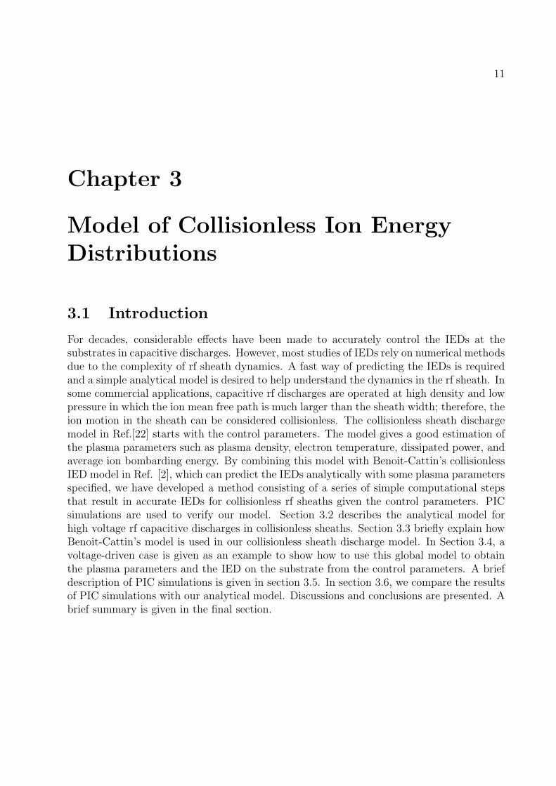
A semianalytical model [45] can be employed to estimate the IED. Figure 3.1 shows thescheme of this model. Besides the control parameters from the tool measurements, thismodel needs the sheath response from PIC simulations. The sheath voltage Vs(t) (bluedash curve in the upper figure) is collected for a few rf periods from the PIC simulationafter steady state. Fourier transforming Vs(t), we get Vs(f) (blue dash curve in the lowerfigure), where f is the frequency. Applying a filter α(f) to Vs(f) (getting the black curvein the lower figure) and doing an inverse Fourier transform, we get the voltage seen by ionsVi(t) (black curve in the upper figure). In Ref. [45], the filter function was chosen to beα(f) = [(c2πfτion)

q + 1]−1/q with c = 0.3 × 2π and q = 5. Since the IED within a certainsmall energy interval is proportional to the total time for Vi(t) to lie within that energyinterval, Vi(t) is converted into an IED as f(Ei) ∝ |dVi/dt|−1. This model is capable ofdealing with both single and multiple- frequency driven rf sheaths, so long as the ion transittime τion ≪ 1/f .

Figures 3.2 and 3.3 show the time-averaged temperature and number density for ions(dashed line) and electrons (solid line) for Vrf = 500 V at 13.56 MHz, with other controlparameters remaining the same. The averaging time is eight rf periods. A fairly MaxwellianEEDF is observed. The sheath region can be identified from the sharp drop of the numberdensities and the position where the time-averaged ion and electron number densities branch,suggesting the maximum position of the oscillating sheath edge, or the ion sheath width sm.To recognize the sheath edge in simulations, the sheath edge is determined by the positionat which the ratio of simultaneous electron and ion number densities reaches 0.8. Thisfactor is a reasonable value considering the unavoidable non-physical noise caused by thesimulations, which is still able to reveal the physical definition of the sheath edge, where thecharge neutrality is violated. Besides, the time-averaged values obtained over thousands ofrf periods have reduced the effects of simulation noise by square root of the number of timesin the average. A ratio of 0.6, instead of 0.8 was also used to determine the sheath edge.


Figure 3.1: Scheme for Alan Wu’s semianalytical IED model

A negligible difference, less than 5 %, in the ion sheath width was observed. The sheathwidth, temperatures and number densities of ions and electrons, and the ion flux found bysimulations agree very well with the theoretical values of the analytical model (shown inTable 3.1).

Figure 3.4 presents the IEDs for Vrf = 500 V at 13.56 MHz, obtained from the theoreticalmodel (solid), semianalytical model (dashed) and PIC simulation (dot-dashed). The IEDsfor a current-driven case Irf = 2.05 A are shown in Fig. 3.5. Both the semianalytical andPIC IEDs have a shift of about −20 V compared to the voltage-driven case.

To investigate the sensitivities of the current- and voltage-driven sources on the IEDs,we take the 13.56 MHz, Vrf = 500 V and Irf = 2.05 A cases as benchmarks. We shift thesources by a ±10% amplitude and observe the corresponding effects the IEDs would presenttheoretically (shown in Fig. 3.6), and in PIC simulations (shown in Fig. 3.7). A ±10% shiftis observed for theoretical IEDs for the voltage-driven cases (shown in Fig. 3.6 on bottom),while the current-driven cases show a larger shift, ± 12.5% with the same 10% variationof the source amplitude. For the IEDs from PIC simulations, the current-driven cases alsoshow larger shifts, ± 12%, given that the peak ion bombarding energy is about 20 V lowerthan that for the corresponding voltage-driven case.

The difference of the sensitivities of the IEDs to current or voltage sources can be well-


explained by the theoretical model, as follows: With the same shift of the source, the shiftof the IED is determined by the shift of the sheath voltage V1. For the voltage-drivendischarge, V1 ∝ Vrf , the source voltage. For the current-driven discharge, with Sstoc ≫ Sohm,substituting Eq. (3.6) into Eq. (3.10) yields ns ∝ V1. Using this in the Child law Eq. (3.12)

gives sm ∝ V1/41 . Using this in Eq. (3.8) gives V1 ∝ J

4/31 . Hence, a 10% shift in J1 produces

a 13.3% shift in V1. In other words, IEDs are less sensitive to voltage-driven sources than tocurrent-driven sources under the same conditions.

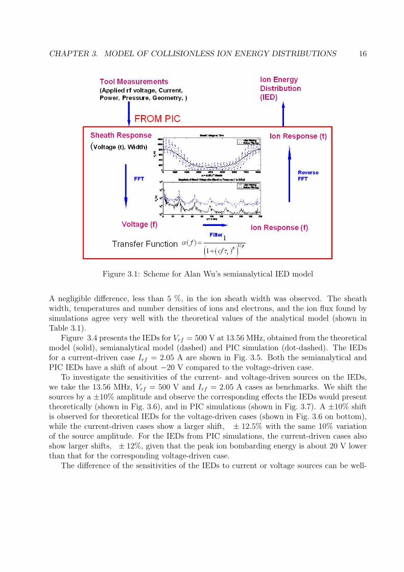
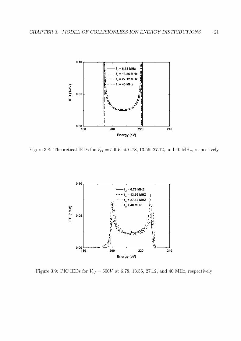
Finally, we investigate the effects of the rf frequency on the IED for a fixed rf voltage-driven source amplitude. Four cases are examined: 6.78 MHz, 13.56 MHz, 27.12 MHz, and40 MHz. Both results from theories (shown in Fig. 3.8) and PIC simulations (shown inFig. 3.9) show a surprising independence of the IEDs on the rf frequency. From Eq. (3.2) wecan see, for a fixed source amplitude, that the ion energy spread △Ei is determined by theproduct of the sheath width sm and the rf frequency. Varying the rf frequency changes thedischarge steady states accordingly, with completely different electron temperature, numberdensities, etc, as shown in Table 3.1. Substituting Eq. (3.6) into Eq. (3.10) shows thatns ∝ ω2 at fixed voltage. Substituting this into the Child law Eq. (3.12) yields sm ∝ ω−1.Hence the product smω=const at fixed source voltage. Hence we find that no matter howthe frequency varies, the ion energy spread given in Eq. (3.2) remains unchanged. This isseen in Table 3.1; we see that when the frequency doubles, the sheath width halves. Thevalue of ωsm hardly varies, which implies an unchanged IED. Equation (3.2) shows that△Ei is inversely proportional to τion/τrf , which is about 2.2 for all the frequencies. For thecases we examined, the ions respond to an average sheath voltage and τrf/τion becomes thecrucial parameter in determining the shape of the IEDs. An unchanged τion/τrf results inthe independence of IEDs on the rf frequencies.

To sum up, the model provides full calculations of inside-plasma parameters including themean ion bombarding energy with the external control factors (pressure, discharge length,rf voltage or current, and frequency) given.

3.7 Summary

A global model for high voltage rf capacitive discharges in the collisionless sheath regimeis developed. Our model requires only specification of the control parameters, not relyingon intermediate parameters from simulations or experimental measurement. Convincinglyverified by PIC simulations, this model is able to rapidly predict the plasma parameters andthe IEDs. It is a good tool for in-depth understanding of the basic physics of capacitivedischarges in the collisionless sheath regime. It is found that for the same variations of rfsource amplitudes, larger voltage shifts are expected in the IEDs for current-driven thanvoltage-driven cases. We also find that for a fixed rf voltage-driven source amplitude, theIEDs show a surprising independence on the rf frequencies. Our model gives a fast way ofexploring the physics of these plasma processing discharges. The capability of verifying the


0.00 0.02 0.04 0.06 0.08 0.10

0

1

2

3

4

Tim

e-a

ve

rag

ed

Te

mp

era

ture

(V

)

Position (m)

Ti

Te

Figure 3.2: PIC time-averaged temperatures for Vrf = 500V at 13.56 MHz

0.00 0.02 0.04 0.06 0.08 0.10

0.00E+000

1.00E+015

2.00E+015

3.00E+015

Tim

e-a

ve

rag

ed

De

nsity (

m-3)

Position (x)

Time-averaged ion density

Time-averaged electron density

Figure 3.3: PIC time-averaged densities for Vrf = 500V at 13.56 MHz


160 180 200 220 240 2600.0

0.1

0.2

IED

(1/e

V)

Energy (eV)

Theoretical Semianalytical PIC

Figure 3.4: Theoretical, semianalytical, and PIC IEDs for Vrf = 500V at 13.56 MHz

160 180 200 220 240 2600.0

0.1

0.2

IED

(1/e

V)

Energy (eV)

Theoretical Semianalytical PIC

Figure 3.5: Theoretical, semianalytical, and PIC IEDs for Irf = 2.05A at 13.56 MHz


140 160 180 200 220 240 2600.00

0.05

0.10

140 160 180 200 220 240 2600.00

0.05

0.10

Energy (eV)

IED

(1/e

V)

Irf = 1.85 A Irf = 2.05 A Irf = 2.26 A

Energy (eV)

IED

(1/e

V)

Vrf = 450 V Vrf = 500 V Vrf = 550 V

Figure 3.6: Theoretical IEDs for current-driven (top) and voltage-driven (bottom) dischargesat 13.56 MHz

140 160 180 200 220 240 2600.00

0.05

0.10140 160 180 200 220 240 260

0.00

0.05

0.10

IED

(1/e

V)

Energy (eV)

Vrf = 450 V Vrf = 500 V Vrf = 550 V

Energy (eV)

IED

(1/e

V)

Irf = 1.85 A Irf = 2.05 A Irf = 2.26 A

Figure 3.7: PIC IEDs for current-driven (top) and voltage-driven (bottom) discharges at13.56 MHz


180 200 220 2400.00

0.05

0.10

IED

(1/e

V)

Energy (eV)

frf = 6.78 MHz frf = 13.56 MHz frf = 27.12 MHz frf = 40 MHz

Figure 3.8: Theoretical IEDs for Vrf = 500V at 6.78, 13.56, 27.12, and 40 MHz, respectively

180 200 220 2400.00

0.05

0.10

IED

(1/e

V)

Energy (eV)

frf = 6.78 MHZ frf = 13.56 MHZ frf = 27.12 MHZ frf = 40 MHZ

Figure 3.9: PIC IEDs for Vrf = 500V at 6.78, 13.56, 27.12, and 40 MHz, respectively


model by PIC simulations on a highly accurate level suggests that the model can be extendedto investigate multifrequency capacitive discharges, the collisional sheath regime, and otherinteresting topics in plasma processing.


Table 3.1: Theoretical and Simulation Discharge Parameters

Vrf , Irf f Te TePIC εc sm n0 n0PIC ns Γ ΓPIC εi △Ei

500 V 6.78 3.57 3.56 59 0.0218 6.0E14 6.12E14 2.14E14 6.28E17 6.39E17 208 27.4500 V 13.56 3.31 3.30 64 0.0113 2.52E15 2.56E15 8.30E14 2.34E18 2.39E18 208 26.4500 V 27.12 3.20 3.16 67 0.0057 1.03E16 1.06E16 3.26E15 9.05E18 9.17E18 208 26.2500 V 40 3.17 3.14 67 0.0036 2.25E16 2.30E16 7.05E15 1.95E19 1.98E19 208 25.9450 V 13.56 3.30 3.30 64 0.0110 2.28E15 2.30E15 7.48E14 2.11E18 2.15E18 187 23.2550 V 13.56 3.31 3.30 64 0.0116 2.76E15 2.82E15 9.11E14 2.57E18 2.62E18 228 29.81.85 A 13.56 3.30 3.23 64 0.0110 2.22E15 2.30E15 7.28E14 2.05E18 2.09E18 182 22.42.05 A 13.56 3.31 3.24 64 0.0113 2.52E15 2.60E15 8.30E14 2.34E18 2.39E18 207 26.42.26 A 13.56 3.31 3.24 64 0.0116 2.83E15 2.93E15 9.34E14 2.64E18 2.69E18 234 30.8

Vrf , Irf - source in V, A; f - rf frequency in MHz; Te - electron temperature in V; εc -collisional energy loss per electron-ion pair created in V; sm - sheath width in m; n0 -number density at the center in m−3; ns - number density at the sheath edge in m−3; Γ -ion flux in the sheath in m−2s−1; εi - ion energy hitting the electrode in V; △Ei - ion energyspread in V; PIC in the subscript denotes the discharge parameters by simulations.

24

Chapter 4

Collisional Sheath Model with EnergyDependent λi

4.1 Introduction

In most of the existing collisional sheath models, the ion mean free path λi is a constant.For a typical capacitive rf discharge, the energy that ions pick up as they traverse acrossthe sheath can range from zero to hundreds of volts. The cross section, or the collisionalprobability of the ion-neutral charge exchange reactions highly differs with such a wide energyrange of ions. It is necessary to take into account the energy dependence of λi in order toachieve accurate estimation of the plasma parameters within the sheath. The work in thischapter is based on Lieberman’s collisional sheath model[22], with an energy dependent ionmean free path in the form of λi = λ0(vi/v0)

b. Here, λ0 is defined as the ion mean freepath at a reference velocity v0. This updated collisional sheath model gives an analytical,self-consistent solution for a collisional sheath driven by a sinusoidal, RF current source. Thebasic equations and derivations are presented in Section 4.2. The effective sheath capacitanceand conductance is determined in Section 4.3 and 4.4. We give an example in Section 4.5,showing some important plasma parameters for varying energy dependence of the ion meanfree path. By setting the factor of b to zero, the model can reproduce the results in Ref.[22].A brief summary is given in the final section.

4.2 Basic Equations

The derivations are based on Ref.[21, 22]. The Maxwell equation for the instantaneous electricfield E(x, t) within the sheath is

∂E

∂x=

e

ϵ0ni(x), s(t) < x

= 0, s(t) > x. (4.1)

CHAPTER 4. COLLISIONAL SHEATH MODEL WITH ENERGY DEPENDENT λI 25

Here, s(t) is the distance from the ion-sheath boundary at x = 0 to the electron-sheathedge. ϕ is defined as: s(t) = x for ωt = ±ϕ.

The equations for the time-average electric field E(x) and potential Φ(x) are:

dE

dx=

e

ϵ0(ni(x)− ne(x)) (4.2)

dΦ

dx= −E (4.3)

The equation for the electron-sheath motion is obtained by equating the displacementcurrent to the conduction current at the electron-sheath edge:

−eni(s)ds

dt= −J0 sinωt (4.4)

We integrate Eq. 4.1 to obtain

E =e

ϵ0

∫ x

sni(ζ)dζ, s(t) < x

= 0, s(t) > x. (4.5)

We integrate Eq. 4.4 to obtain

e

ϵ0

∫ s

0ni(ζ)dζ =

J0ϵ0ω

(1− cosωt) (4.6)

where we have chosen the integration constant so that s(t) = 0 at ωt = 0. From Eq. 4.5 andEq. 4.6 we obtain

E(x, ωt) =e

ϵ0

∫ x

0ni(ζ)dζ −

J0ϵ0ω

(1− cosωt), s(t) < x

= 0, s(t) > x. (4.7)

Inserting Eq. 4.6 with s = x, ωt = ϕ into Eq. 4.7 we obtain the instantaneous and time-average electric fields:

E(x, ωt) =J0ϵ0ω

(cosωt− cosϕ), s(t) < x

= 0, s(t) > x. (4.8)

and

E =J0

ϵ0ωπ(sinϕ− ϕ cosϕ) (4.9)


The ion particle conservation equation is,

nivi = n0uB (4.10)

The ion momentum conservation equations for collisionless and collisional rf sheaths are,respectively,

1

2Mv2i =

1

2u2B − eΦ (4.11)

vi = µiE =2eλi

πMviE (4.12)

Here, µi is the mobility and E is the time-averaged electric field. By assuming λi =λ0(vi/v0)

b, with λ0 the ion mean free path at reference ion velocity v0 at ion temperatureTi = 0.05 V , we have Eq. 4.12 modified for the energy dependent λi as follows:

vi =2eλ0

(viv0

)bπMvi

E (4.13)

Therefore, we have

v2−bi =

2eλ0v−b0

πME (4.14)

By substituting vi in Eq. 4.10 with the above expression, we get

ni = n0uB

(2eλ0E

πMv−b0

)− 12−b

(4.15)

For a constant λi, b = 0. By setting b = 0 in Eq. 4.15, we obtain the same expression ofni as in Ref.[22].

Inserting Eq. 4.15 into Eq. 4.4 with s = x, ωt = ϕ, we obtain

dϕ

dx=

uB

s0

(πM

2eλ0

) 12−b

vb

2−b

0

1

E1

2−b sinϕ(4.16)

wheres0 = J0/(eωn0) (4.17)

is an effective oscillation amplitude.Again, by setting b = 0 in Eq. 4.16, we obtain the same expression of dϕ/dx as in Ref.[22]

for a constant λi in a collisional rf sheath.Inserting Eq. 4.9 into Eq. 4.16 and integrating, we obtain

x

s0= H

∫ ϕ

0(sin ζ − ζ cos ζ)

12−b sin ζdζ (4.18)


0 50 1000

1

2

3

4

5

H/H0

H0

b = 0 b = 0.1 b = 0.2 b = 0.3 b = 0.4

Figure 4.1: H/H0 versus H0 for varying b

where

H =

(2λ0s0π2

e2n0

ϵ0M

) 12−b

v− b

2−b

0

(M

eTe

)1/2

(4.19)

By setting b = 0 in Eq. 4.19, we obtain

H0 =

(2λ0s0π2λ2

D

)1/2

(4.20)

with λD = (ϵ0Te/en0)1/2, the same as in Ref.[22] for a constant λi in a collisional rf sheath.

The effects of b on the value of H are shown in Fig. 4.1. As we will see from the laterderivation, H is a factor that appears in almost all the expressions of the important plasmaparameters. The discrepancy of H (the energy dependent λi case) from H0 (the constant λi

case) gets larger as the value of H0 increases. It is also shown very clearly in Fig. 4.2 thatthis discrepancy increases with b. Therefore, for the collisional rf discharges with a high H0,it is required to consider the energy dependence of λi. Making the simplifying assumptionof a constant λi would achieve inaccurate results.

Comparing Eq. 4.19 with Eq. 4.20, we get

H = H2

2−b

0

(uB

v0

) b2−b

(4.21)

Setting x = s(t) and ϕ = ωt in Eq. 4.18, we obtain the nonlinear oscillation motionof the electron sheath, which is shown in Fig. 4.3 with x normalized by H (top) and H0


0.0 0.2 0.4

1.0

1.5

2.0

H/H

0

b

Figure 4.2: H/H0 versus b

(bottom), respectively. As we can see from Eq. 4.18, H behaves the same for the energydependent λi case as H0 does for the constant λi case in Ref.[22]. The effects of b on x comefrom two parts: H and the integrand (b in the exponent). The top plot with x normalizedby H shows that the effects of b in the integrand is very small. This implies that, byonly updating the value of H from the constant λi case while keeping the integrand (also baffected) remaining unchanged in Eq. 4.18, it is convenient and appropriate to obtain x forthe energy dependent λi case from the constant λi case. From the bottom plot in Fig. 4.3we can also see the necessity of considering λi as an energy dependent function.

Setting s = sm at ϕ = π in Eq. 4.18, we obtain the ion-sheath thickness as a functionof b numerically. Define the coefficients Csm and C ′

sm: sm = CsmH0s0 = C ′smHs0, with

Csm = C ′sm = Csm0 for b = 0. The normalized Csm (bottom) and C ′

sm (top) for varyingb are shown in Fig. 4.4. The ion-sheath thickness in the collisional sheaths for an energydependent λi is listed in Eq. 4.22 for various b values, with b = 0 representing the case for aconstant λi [22].

sm = 1.92H0s0 = 1.92Hs0, b = 0

= 2.16H0s0 = 1.93Hs0, b = 0.1

= 2.46H0s0 = 1.95Hs0, b = 0.2

= 2.84H0s0 = 1.97Hs0, b = 0.3

= 3.35H0s0 = 1.99Hs0, b = 0.4. (4.22)


0

1

2

0.00 1.57 3.14

0.00 1.57 3.140

1

2

3

4

x/(Hs0)

b =0 b = 0.1 b = 0.2 b = 0.3 b = 0.4

x/(H0s0)

Figure 4.3: Normalized position versus phase for varying b

1.000

1.025

1.0500.0 0.2 0.4

0.0 0.2 0.41.0

1.2

1.4

1.6

1.8

Csm

'/Csm

0

Csm

/Csm

0

b

Figure 4.4: Normalized Csm versus b


0.0 0.2 0.4

0.8

1.0

1.2

Cs0

b

Figure 4.5: Cs0 versus b

For a given discharge, H0 is a constant, whileH is variable, dependent on the value of b. Inother words, choosing different energy dependences of ion-neutral mean free path (differentb) will result in different relations of the ion-sheath thickness, which, for a self-consistentmodel, will result in different plasma parameters.

Substituting Eq. 4.19 in the above expression for sm and solving for s0, we obtain

s0 = 1.10λ2/3D s2/3m /λ

1/30 , b = 0

= 1.02λ2/3D s2/3m /λ

1/30 , b = 0.1

= 0.93λ2/3D s2/3m /λ

1/30 , b = 0.2

= 0.85λ2/3D s2/3m /λ

1/30 , b = 0.3

= 0.76λ2/3D s2/3m /λ

1/30 , b = 0.4. (4.23)

Define the coefficient Cs0: s0 = Cs0λ2/3D s2/3m /λ

1/30 . Cs0 for varying b is plotted in Fig. 4.5.

The time-average electric field is given by Eq. 4.9 with ϕ(x) obtained from Eq. 4.16. E forvarying b is plotted in Fig. 4.6. The ion density ni(x) in Eq. 4.15 for varying b is plotted inFig. 4.7.

The time-average potential is found by inserting Eq. 4.9 into Eq. 4.3 and integrating,which yields

Φ = − J0πϵ0ω

∫ ϕ


dx

dζdζ (4.24)

Using Eq. 4.16 along with Eq. 4.9 and Eq. 4.17 in Eq. 4.24, we obtain


0.00 0.01 0.020

1

2

3

4

E/(en0s0/ )

x (m)

b = 0 b = 0.1 b = 0.2 b = 0.3 b = 0.4

Figure 4.6: Normalized dc electric field versus position for varying b

0.00 0.01 0.020

1

2

n i/n0

x (m)

b = 0 b = 0.1 b = 0.2 b = 0.3 b = 0.4

Figure 4.7: Normalized ion density ni/n0 versus position for varying b


0.00 0.01 0.020

200

400

Nor

mal

ized

dc

pote

ntia

l -/T

e

x (m)

b = 0 b = 0.1 b = 0.2 b = 0.3 b = 0.4

Figure 4.8: Normalized dc potential Φ/Te versus position for varying b

Φ

Te

= −H

π

s20λ2D

∫ ϕ


3−b2−b sin ζdζ (4.25)

The total dc voltage across the sheath can be obtained by setting ϕ = π and Φ = −V in Eq.4.25 and evaluating the integral numerically, which is shown in Fig. 4.8.

The total dc voltage across the sheath is related to the dc ion current and the ion sheaththickness by an expression in the form of Child’s law:

Ji = Kϵ0

(2e

M

)1/2 V 3/2

s2m(4.26)

where Ji = en0uB is the dc ion current and V = −Φ(ϕ = π) is the voltage across the sheath.Setting ϕ = π and Φ = −V in Eq. 4.25 and evaluating the integral numerically, we obtainV for different values of b:

V

Te

= 3.15H0

π

s20λ2D

= 3.15H

π

s20λ2D

, b = 0

= 3.58H0

π

s20λ2D

= 3.21H

π

s20λ2D

, b = 0.1

= 4.12H0

π

s20λ2D

= 3.27H

π

s20λ2D

, b = 0.2


1.00

1.05

1.100.0 0.2 0.4

0.0 0.2 0.41.0

1.5

2.0

CV'/C

V0

CV/C

V0

b

Figure 4.9: Normalized CV versus b

= 4.83H0

π

s20λ2D

= 3.34H

π

s20λ2D

, b = 0.3

= 5.77H0

π

s20λ2D

= 3.43H

π

s20λ2D

, b = 0.4. (4.27)

Define the coefficients CV and C ′V :

VTe

= CVH0

π

s20λ2D= C ′

VHπ

s20λ2D, with CV = C ′

V = CV 0 at b = 0.

The normalized CV and C ′V for varying b is plotted in Fig. 4.9.

Using Eq. 4.19 and Eq. 4.17 in Eq. 4.27 and the definitions for λD and Ji, we obtainEq. 4.26 with

K = π3/2/21/2(Csm/(CVCs0))3/2(λ0/sm)

1/2 (4.28)

For collisionless ion motion in the sheath [21], the self-consistent result is Kf = 0.82. Forcollisional ion motion with the energy dependent λi, we get

K = 1.62(λ0/sm)1/2, b = 0

= 1.79(λ0/sm)1/2, b = 0.1

= 2.03(λ0/sm)1/2, b = 0.2

= 2.27(λ0/sm)1/2, b = 0.3

= 2.63(λ0/sm)1/2, b = 0.4. (4.29)


4.3 Sheath Capacitance

Integrating Eq. 4.8 with respect to x, we obtain the instantaneous voltage from the plasmato the electrode across the sheath:

V (t) =∫ sm

sE(x, t)dx. (4.30)

Changing variables from x to ϕ and using Eq. 4.8, we obtain

V (t) =J0ϵ0ω

∫ π

ωt(cosωt− cosϕ)

dx

dϕdϕ. (4.31)

Using Eq. 4.9 and Eq. 4.16 to evaluate dx/dϕ in Eq. 4.31 we obtain, for 0 < ωt < π,

V (t) =(en0s

20/ϵ0

)H∫ π

ωt(cosωt− cosϕ) (sinϕ− ϕ cosϕ)

12−b sinϕdϕ. (4.32)

V (t) is an even, periodic function of ωt with period 2π. For −π < ωt < π, V (t) is givenby the right hand side of Eq. 4.32 with ωt replaced by −ωt. Figure 4.10 shows the sheathvoltage versus ωt normalized with H (top) and H0, respectively for varying b. The peakvalue of V (t) occurs at ωt = 0:

V (0) = 2.50H0(en0s20/ϵ0) = 2.50H(en0s

20/ϵ0), b = 0

= 2.83H0(en0s20/ϵ0) = 2.54H(en0s

20/ϵ0), b = 0.1

= 3.25H0(en0s20/ϵ0) = 2.58H(en0s

20/ϵ0), b = 0.2

= 3.80H0(en0s20/ϵ0) = 2.63H(en0s

20/ϵ0), b = 0.3

= 4.52H0(en0s20/ϵ0) = 2.68H(en0s

20/ϵ0), b = 0.4. (4.33)

By setting V (0) = C ′V mH(en0s

20/ϵ0) = CV mH0(en0s

20/ϵ0), with CV m = CV m0 at b = 0, we

plot the normalized coefficient in the peak sheath voltage C ′V m/CV m0 and CV m/CV m0 versus

b in Fig. 4.11. Expanding V (t) in a Fourier series

V (t) =∞∑k=0

Vk cos kωt (4.34)

for b = 0, we obtain the same result as in Ref.[22]:

V0 = V = 1.00H(en0s20/ϵ0),

V1 = 1.28H(en0s20/ϵ0),

V2 = 0.25H(en0s20/ϵ0),

V3 = −0.034H(en0s20/ϵ0). (4.35)


0

1

2

30.00 1.57 3.14

0.00 1.57 3.140

1

2

3

4

5

V/H*(0/e2n

0s

02)

b = 0 b = 0.1 b = 0.2 b = 0.3 b = 0.4

V/H0*(

0/e2n

0s

02)

t

Figure 4.10: Normalized sheath voltage versus phase for varying b

1.00

1.05

1.100.0 0.2 0.4

0.0 0.2 0.41.0

1.5

2.0

CV

m'/C

Vm

0

CV

m/C

Vm

0

b

Figure 4.11: Normalized CV m versus b


Results for varying b are shown in Table 4.1.The effective capacitance per unit area is defined from the relation

−J0 sinωt = C ′s

d

dt(V1 cosωt) (4.36)

. Using Eq. 4.17 along with the relation of sm = C ′smHs0 and V1 = C ′

1H(en0s20/ϵ0), we get

C ′s =

C ′sm

C ′1

ϵ0sm

(4.37)

with C ′s = 1.52ϵ0/sm for b = 0 and C ′

s = 1.44ϵ0/sm for b = 0.4. The value of the coefficientin this relation decreases as b increases. For collisionless ion motion in the sheath [21], thecoefficient is 1.23.

4.4 Sheath Conductance

Follow the procedure in Ref.[22] to calculate the sheath conductance in a collisional sheathwith varying b. The expression of the sheath velocity us = ds/dt is generalized as

us = u0H(sinϕ− ϕ cosϕ)1/(2−b) sinϕ (4.38)

Here, u0 is the amplitude of the oscillation velocity of the plasma electrons u0(t) at theion-sheath edge x = 0, nsus = u0n0 sinϕ. The dc power transferred to the electrons per unitarea is given by S = 4mΓsn

−10 ⟨(us − u0)usns⟩ϕ. Here, Γs is the electron-flux incident on the

ion-sheath edge. For a Maxwellian distribution, Γs = 14n0ue with ue = (8eTe/πm)1/2 the

mean electron speed. Doing the substitution in S, we obtain

S = Hmn0ueu20⟨(sinϕ− ϕcosϕ)1/(2−b) sinϕ2⟩ϕ (4.39)

Set S = C ′SHmn0ueu

20, we get C ′

S for varying b: C ′S = 0.491, 0.493, 0.496, 0.5, 0.503

for b = 0, 0.1, 0.2, 0.3, 0.4, respectively. The effective surface conductance per unit area isdefined

G′s =

J20

2S(4.40)

where J0 = en0u0.Taking Eq. 4.39 into Eq. 4.40 we obtain

G′s =

1

2C ′SH

(e2n0

mue

)(4.41)

Using Eq. 4.21, Eq. 4.20, and s0 = Cs0λ2/3D s2/3m /λ

1/30 , we obtain

H =(2Cs0

π2

) 12−b

(λ0smλ2D

) 23(2−b) (uB

v0

) b2−b

(4.42)


For b = 0, the coefficient(2Cs0

π2

) 12−b in Eq. 4.42 is 0.47. This result agrees with the constant

ion mean free path case (see Eq. 38, [22]).Using Eq. 4.42 and Eq. 4.41 we then obtain

G′s =

1

2C ′S

(π2

2Cs0

) 12−b ( v0

uB

) b2−b

(λ2D

λ0sm

) 23(2−b)

(e2n0

mue

)(4.43)

As we can see from the above derivations that, the expressions of the plasma parametersfor an energy dependent λi case, for example, the oscillating sheath edge x and the sheathvoltage V , can be updated from the constant λi case [22] by two procedures: modifyingH using Eq. 4.21; adding the b related power to the integrand, as shown in Eq. 4.18 forthe oscillating sheath motion and Eq. 4.32 for the sheath voltage. The effect of b on themodification of H is always large, as the primary b-effect carrier; while the other carrier, bin the integrand, can be negligible for some parameters (i.e., sheath motion) and preferablyretained (i.e., sheath voltage).

4.5 Example

As an example, we choose J0 = 32 A/m2, p = 40 mTorr, ω = 2π× 13.56 MHz, Te = 2.5 eV,n0 = 8.5 × 1014 m−3, and M = 40 amu (i.e., argon). J0 is the amplitude of the rf currentdensity passing through the sheath; n0 is the plasma density at the ion-sheath edge. Thenwe obtain λD = 4.03× 10−3 m, uB = 2.44× 103 m/s, ue = 1.06× 106 m/s, Ji = 0.33 A/m2,s0 = 2.76 × 10−3 m, v0 = 4.89 × 102 m/s, and λ0 = 7.58 × 10−4 m. ue is the mean electronspeed; Ji is the dc ion current; s0 is the effective oscillation amplitude; λ0 is the reference ionmean free path at the reference velocity v0 (at Ti = 0.05 eV). For varying b, some parametersare shown in Table 4.2. As the value of b increases, λi within the sheath gets larger, whichis more closer to a collisionless sheath case. As shown in the change of C ′

s and G′s for the

increasing b, the sheath capacitance and conductance decreases.

4.6 Summary

An updated analytical, self-consistent model for collisional, capacitive RF sheaths with theenergy dependent ion mean free path λi is developed, based on the model in Ref. [22] with aconstant ion mean free path. The effects of the energy dependence of the ion mean free pathare studied for various plasma parameters within the sheath. A simple method of generalizingthe model with the constant λi to one with the energy dependent λi is demonstrated. Bysetting the energy dependence term b to zero (a constant λi), this model is successfullyrestored to the model in Ref. [22].


Table 4.1: Coefficients of Fourier Series Expansion of V (t) for Varying bVk = C ′

kH(en0s20/ϵ0) = CkH0(en0s

20/ϵ0)

b C ′0 C ′

1 C ′2 C ′

3

0 1.00 1.28 0.25 -0.0340.1 1.02 1.30 0.25 -0.0350.2 1.04 1.33 0.25 -0.0370.3 1.06 1.35 0.25 -0.0390.4 1.09 1.38 0.25 -0.041

b C0 C1 C2 C3

0 1.00 1.28 0.25 -0.0340.1 1.14 1.46 0.28 -0.0390.2 1.31 1.67 0.31 -0.0470.3 1.54 1.96 0.36 -0.0570.4 1.84 2.33 0.42 -0.070

Table 4.2: Some Parameters for Varying b

b H sm V K V (0) V1 V2 V3 C ′s G′

s S Si

0 1.61 0.86 190 0.48 473 242 47.3 -6.43 0.15 1.43E-3 3.6E-3 6.3E-30.1 1.80 0.96 216 0.50 535 276 53.0 -7.38 0.14 1.27E-3 4.0E-3 7.2E-30.2 2.04 1.10 248 0.53 615 316 58.7 -8.89 0.12 1.12E-3 4.6E-3 8.2E-30.3 2.33 1.27 291 0.56 719 371 68.1 -10.8 0.10 9.70E-4 5.3E-3 9.7E-30.4 2.72 1.49 348 0.59 855 441 79.5 -13.2 0.087 8.26E-4 6.2E-3 1.2E-2

sm - ion sheath thickness in cm; V - dc voltage across the sheath in V; K - coefficient inChild’s law (Eq. 4.26); V (0) - peak value of sheath voltage in V; V1, V2, and V3 - first,

second, and third harmonic of sheath voltage in V; C ′s - sheath capacitance in pF/cm2; G′

s

- sheath conductance in S/cm2; S - average power transferred to electrons per unit area inW/cm2; Si - dc ion power flux incident on electrode in W/cm2.

39

Chapter 5

IEDs in Collisional, Capacitive RFSheath

5.1 Introduction

At high operating pressures, the rf sheaths are typically collisional with the ion mean freepath much smaller than the sheath width. While traversing the sheath, ions have collisionswith neutrals. Through an ion-neutral charge exchange collision, the ion is neutralized bypicking up a unit charge from the neutral, and cannot be accelerated by electric field anymore. The neutral loses a negative unit charge and becomes a secondary ion, with an initialenergy of order the thermal energy of the background gas. The secondary ion then getsaccelerated by the electric field. The final kinetic energy that an ion can carry to the substrateis smaller than the sheath voltage drop. Instead, their bombarding energy is determined bythe position where their last collision takes place. The ion-neutral elastic scattering alsocontributes to the spread of the IED, as the kinetic energy that the primary ion carriesgets redistributed angularly. During these processes, the electron-sheath edge is oscillatingback and forth. Secondary ions generated by ion-neutral charge exchange collisions maybe created within the space-charge region (between the instantaneous sheath edge and theelectrode surface) or within the zero electric field region. Ions born within the space-chargeregion are accelerated immediately by the electric field in the sheath, while those born withinthe zero electri field region remain at rest until the oscillating sheath passes by. These ionsexperience a delay in their movement towards the electrode, which makes multiple peaksin the final IED. Due to ion-neutral collisions, combined with the effects of the oscillatingsheath, the IED is broad and has multiple peaks at low energies.

The ion mean free path λi = 1/ngσ is a characteristic parameter in evaluating thecollisional degree within the sheath. Here, ng is the number density of neutrals, and σis the cross section of the ion-neutral collision. Most of the existing models and numericalcalculations of collisional rf sheaths assume λi is a constant, in order to simplify the problem.

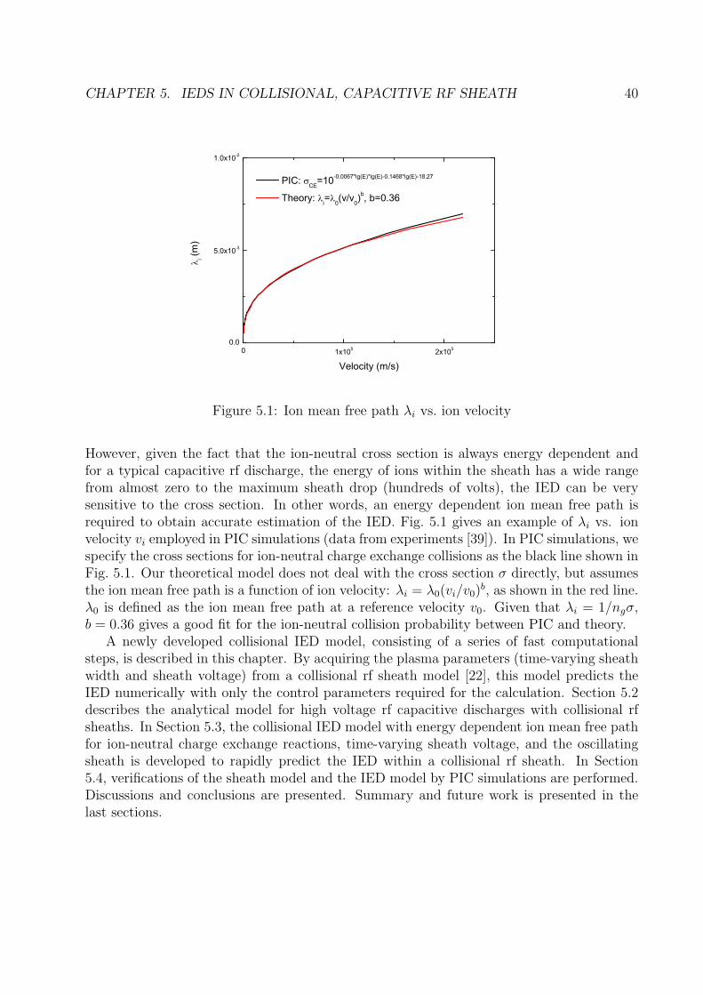
CHAPTER 5. IEDS IN COLLISIONAL, CAPACITIVE RF SHEATH 40

0 1x105 2x1050.0

5.0x10-3

1.0x10-2

i (m)

Velocity (m/s)

PIC: CE=10-0.0067*lg(E)*lg(E)-0.1468*lg(E)-18.27

Theory: i= 0(v/v0)b, b=0.36

Figure 5.1: Ion mean free path λi vs. ion velocity

However, given the fact that the ion-neutral cross section is always energy dependent andfor a typical capacitive rf discharge, the energy of ions within the sheath has a wide rangefrom almost zero to the maximum sheath drop (hundreds of volts), the IED can be verysensitive to the cross section. In other words, an energy dependent ion mean free path isrequired to obtain accurate estimation of the IED. Fig. 5.1 gives an example of λi vs. ionvelocity vi employed in PIC simulations (data from experiments [39]). In PIC simulations, wespecify the cross sections for ion-neutral charge exchange collisions as the black line shown inFig. 5.1. Our theoretical model does not deal with the cross section σ directly, but assumesthe ion mean free path is a function of ion velocity: λi = λ0(vi/v0)

b, as shown in the red line.λ0 is defined as the ion mean free path at a reference velocity v0. Given that λi = 1/ngσ,b = 0.36 gives a good fit for the ion-neutral collision probability between PIC and theory.

A newly developed collisional IED model, consisting of a series of fast computationalsteps, is described in this chapter. By acquiring the plasma parameters (time-varying sheathwidth and sheath voltage) from a collisional rf sheath model [22], this model predicts theIED numerically with only the control parameters required for the calculation. Section 5.2describes the analytical model for high voltage rf capacitive discharges with collisional rfsheaths. In Section 5.3, the collisional IED model with energy dependent ion mean free pathfor ion-neutral charge exchange reactions, time-varying sheath voltage, and the oscillatingsheath is developed to rapidly predict the IED within a collisional rf sheath. In Section5.4, verifications of the sheath model and the IED model by PIC simulations are performed.Discussions and conclusions are presented. Summary and future work is presented in thelast sections.


5.2 Collisional, Capacitive RF Sheath Model

In 1989, a simple analytical model of a collisional rf sheath was developed [22]. This modelprovides a self-consistent solution for the dynamics of a high-voltage, capacitive rf sheathdriven by a sinusoidal current source. The ion motion is collisional, with the ion meanfree path λi a constant within the sheath. It is assumed that the ions only respond to thetime-averaged electric field, while the electrons respond to the instantaneous electric field.The ions enter the sheath with a Bohm velocity uB = (eTe/M)1/2, with Te the electrontemperature (in Volts). Given the control parameters of a capacitive rf discharge, this modelgives the time-averaged electric field and potential within the sheath, the nonlinear oscillationof the electron sheath boundary, and the nonlinear oscillating sheath voltage.

5.2.1 Example

Here is an example to explain how this collisional rf sheath model works to obtain the plasmaparameters needed by the IED model. The capacitive rf discharge is driven by a singlefrequency voltage source V (t) = Vrf cos(2πft) under pressure p in argon. The distancebetween electrodes is l and the area of the electrodes is A. The parameters used here are asfollows: Vrf = 176 V, f = 81 MHz, p = 20 mTorr, l = 0.024 m, and A = 5.03 × 10−3 m2.Ions are weakly collisional, with sheath width / ion mean free path sm/λ0 ∼ 1.1, ion transittime across sheath / rf period τion/τrf ∼ 10.

Starting with an estimate of the ion sheath thickness sm ≈ 0.0017 m, and using λi =1/330p (p in Torr, λ in cm) at 300K, the ion mean free path in the sheath is λi = 0.0015 m.The plasma length d ≈ l − 2sm = 0.0206 m. λi/d = 0.0736, which is in the intermediatemean free path regime. The ratio between the edge density and center density is given by

hl ≡ns

n0

≈ 0.86(3 +d

2λi

)−1/2 (5.1)

We have ns/n0 = 0.2747. From 1ngdeff

= 2ngd

ns

n0where ng = 3.3 × 1016p (p in Torr, ng

in cm−3), we get ngdeff = 2.47 × 1019 (in m−2). Solving the particle balance usingFig. 10.1 (Te versus ngdeff for Maxwellian electrons in argon), or numerically, using therate coefficient of reaction 2 in Table 3.3 in Ref. [23], we find Te ≈ 2.8 V. This givesuB = (eTe/M)1/2 ≈ 2.59× 103 m/s. Introduce a coefficient H,

H = (2λis0π2λ2

D

)1/2 (5.2)

where s0 = J1/(eωns), J1 is given by

J1 ≈ 1.52ωϵVrf

2

1

sm(5.3)


The sheath voltage can be written as a Fourier series

Vs(t) =∞∑k=0

Vk cos(kωt) (5.4)

with V0 = V = 1.00H(enss20/ϵ), V1 = 1.28H(enss

20/ϵ), V2 = 0.25H(enss

20/ϵ), V3 = −0.034H(enss

20/ϵ).

The higher harmonics (s > 3) are small and discarded.From Figure 3.17 (εc versus Te) in Ref. [23] where εc is the collisional energy loss per

electron-ion pair created, we get εc ≈ 60 V and εc+ε′e ≈ 80 V, where ε′e is the kinetic energylost per electron lost from the plasma with ε′e ≈ 7.2Te. Estimating νm ≈ Kelng with Kel

given by the rate coefficient of reaction 1 in Table 3.3, we get νm ≈ 6.6× 107 s−1. Then theelectron ohmic heating power per unit area can be obtained by

Sohm ≈

1.73m2e

ns

n0ϵ0ω

2νmT1/2e V

1/21 d if λi ≥ ( Ti

Te)d

1.73m2e

ns

n0ϵ0ω

2νmT1/2e V

1/21

2βln tan(π

4+ βd

4) if λi ≤ ( Ti

Te)d

(5.5)

where cos(βd/2) = ns/n0, V1 is the fundamental rf voltage amplitude across a single sheath.For our parameters, λi ≥ ( Ti

Te)d. Therefore, we obtain Sohm ≈ 63.25 W/m2. For the

stochastic heating power per unit area,

Sstoc ≈ 0.61(m

e)1/2ϵ0ω

2T 1/2e V1 if ωsm ≤ ve (5.6)

We get Sstoc ≈ 449.25 W/m2. Similar to the derivation procedure in the collisionless model,we get ns ≈ 1.58 × 1016 m−3, n0 ≈ 5.74 × 1016 m−3, Ji ≈ 6.00 A/m2, sm ≈ 0.0016 m(very close to the assumed value 0.0017 m), Sabs ≈ 1785.3 W/m2, P = Sabs × A = 8.98 W.The fundamental current density is J1 ≈ 353 A/m2. We have H ≈ 2.94, V ≈ 69.51 V,V1 ≈ 88.97 V, V2 ≈ 17.38 V, V3 ≈ −2.36 V. The averaged ion-bombarding energy εi ≈0.62V λi/sm = 38.03 V. It is noted that V /V1 ≈ 0.78, which agrees with the equation(11.2.56) in Ref. [23].

5.3 Collisional IED Model

5.3.1 Limitation

In this model, electrons are inertialess and respond to the instantaneous electric field; ionsrespond to the time averaged electric field. This model requires: ωpe >> ωrf >> 1/τion.Here, ωpe is the electron plasma frequency, ωrf is the rf frequency, and τion is the ion transittime across one single sheath.

This collisional IED model takes into account ion-neutral charge exchange collisions.Elastic scattering between ions and neutrals is not considered here. The ion-neutral meanfree path is energy dependent, with λi = λ0(v/v0)

b, where λ0 is the ion mean free path


at a reference ion velocity v0 corresponding to an ion temperature Ti = 0.05 V. We useλ0 = 1/(330p) in cm, p in Torr. b is the adjustable power in the λi−v relation, which revealsthe dependence of the charge exchange cross section on energy. For example, b = 0 gives aconstant ion mean free path; the cross section data originally used in OOPD1 gives b = 0.36.The sheath voltage is time-varying, Vs(t) = Vs + Vs sin(ωrf t). Vs is the time averaged sheathvoltage over an rf period. Vs is the amplitude of the oscillating part of sheath voltage.ωrf = 2πf , with f the rf frequency.

In this section, the sheath width s(t) is assumed to be a constant with s(t) = sm,which means that the sheath is not oscillating. In fact, the sheath is oscillating between amaximum thickness of sm and a minimum thickness of a few Debye lengths λDe from theelectrode surface, as we will discuss in a subsequent section.

An expression for the oscillating sheath s(t) is given in Ref. [16]. In their model, ionmotion within the sheath is assumed to be weakly collisional, ion mean free path λi >> sm,and the analysis is restricted to charge exchange collisions.

5.3.2 Scheme

We assume that a constant flux of ions coming from the bulk plasma enters the plasma-sheath edge at x = 0 at Bohm velocity uB; ions are considered as two groups: the uncollidedgroup and the collided group. The uncollided ions bombard the electrode with the totalsheath voltage that they can pick up as they enter the plasma-sheath edge. Ions havingcharge exchange collisions within the sheath pick up the cold neutrals energy Tn and, as thesecondary ions, are accelerated towards the electrode. The energy they take to the electrodeis determined by their last charge exchange collision.

In our model, IEDs contributed from the uncollided and the collided ions are calculatedseparately. The uncollided IED is calculated from Benoit-Cattin’s model[2], which can beconsidered as a collisionless sheath case. The collided IED is calculated from our IED model.Then the two parts of IEDs are combined through normalization of the total IED.

5.3.3 Example

Constant λi, constant Vs

In this case, λi = λ0, Vs(t) = Vs.Let G0 be the flux of ions (ions / m2s) entering the plasma-sheath edge at x = 0. The

total flux that hits the electrode at x = sm without having a collision is

Γ0 = G0e−sm/λ0 (5.7)

Now let Γi(x) be the flux of ions having at least i collisions within the sheath.


Here, the concept of differential flux Γ′i(x) is used. For example, Γ′

1(x) is the flux of ionshaving at least one collision within the sheath. It is known that,

dΓ1(x) = Γ0(x)ngσdx (5.8)

where ng is the neutral density, σ is the cross section of charge exchange collisions, and Γ0(x)is the flux of ions that do not have collisions before x. dΓ1(x) shows the increase of flux ofthe ions that have their first collision at x. Setting λ0 =

1ngσ

, we have

dΓ1(x) = Γ0(x)1

λ0

dx (5.9)

Since dΓ0(x) = −Γ0(x)1λ0dx, we have Γ0(x) = G0e

−x/λ0 . With the initial condition

Γ0 = G0 at x = 0, we get Γ0(x) = G0e−x/λ0 . Therefore, we have

dΓ1 = G0e−x/λ0

1

λ0

dx (5.10)

Thus,

Γ′1(x) =

dΓ1

dx=

1

λ0

G0e−x/λ0 (5.11)

Integrating this differential flux from x = 0 to x = sm yields the total ion flux at theelectrode that has had at least one collision within the sheath.

With the expression of Γ′1(x), we can get Γ′

2(x), Γ′3(x), etc. in a similar way as shown in

the following: Consider a position ξ within the sheath. Γ′1(ξ)dξ, which is dΓ1(ξ), shows the

increase of the flux of ions lying between position ξ and ξ + dξ. These ions have their firstcollision at ξ. This also shows the contribution of the ions transferring from the no-collisiongroup to the at-least-one-collision group.

We have

dΓ2(x) = Γ′2(x)dx =

∫ x

0Γ′1(ξ)

1

λ0

e−(x−ξ)/λ0dξdx (5.12)

Here, Γ′1(ξ)dξ · 1

λ0·dx is the typical expression of ions having collisions between x and x+dx

with 1λ0

as the ’cross section part’ ′ngσ′. The integration is from 0 to x because only when the

first collision happens before x do these ions contribute to dΓ2(x). e−(x−ξ)/λ0 represents the

probability that, after these ions have their first collision at ξ, they don’t have any collisionagain from ξ to x until they reach the position x and have their second collision at x.

Note that we always use dΓ2(x), not Γ2(x). This is because dΓ2(x) shows the changeof the flux of an ion group. Ions that have at least one collision include those having oneand more than one collisions. To move to the question of how many ions have at least twocollisions, we only need to count how many ions that have only one collision have anothercollision. It’s not necessary to count the ions that have already had more than one collision,since this group will surely contribute to the at-least-two-collision group.


The above explanation is to help clarify the following relation between differential fluxand ion energy distribution function. dΓi(x) is the differential flux of ions that have exact icollisions in the sheath, not the ’at-least-i-collision’.

To extend the above equation to the i-th collision differential flux, we have

Γ′i(x) =

∫ x

0Γ′i−1(ξ)

1

λ0

e−(x−ξ)/λ0dξ (5.13)

If at position x, dΓi(x) (which is also Γ′i(x)dx) ions that just have their i-th collision at

x don’t have any collision until they hit the electrode (implying a factor of e−(s−x)/λ), theenergy they will carry to the electrode is what they obtain from being accelerated by theelectric field from x to the electrode.

Γ′i(x)dxe

−(sm−x)/λ0 = −fi(E)dE (5.14)

The index i in fi identifies the contribution of ions having i collisions in the sheath to theIED at the electrode.

For this simple case with constant ion mean free path λ0 and constant sheath voltage Vs,the IED can be obtained analytically by summing up fi:

f(E) =G0smλ0Vs

exp(−smE

λ0Vs

)+G0 exp

(−smλ0

)δ(E − Vs) (5.15)

The first and second terms on the right side of the equation represent the contributionto the IED of the collided ions and uncollided ions, respectively. With the time varyingsheath voltage considered, the second term for the uncollided IED will be expanded from amonoenergetic δ function to a bimodal energy spread function. The corresponding expressionof the uncollided IED from our model with a constant λi and time varying sheath voltageVs(t) = Vs + Vs sin(ωt) agrees with the expression of fE in Benoit-Cattion’s model [2].

It should be noted that, in the above derivation, we use λi to stand for the ion-neutralmean free path for charge exchange reactions. However, if we consider λi as a function ofenergy, λi = λ0(v/v0)

b, λ in the above equations should be specified carefully. Take Eq. 5.13for example. λ in 1

λis the ion mean free path when the ion-neutral charge exchange reaction

takes place at position x, while the λ in e−(x−ξ)/λ is the ion mean free path between ξ and xwhere ions don’t have collisions. In Eq. 5.14, λ in e−(sm−x)/λ is the ion mean free path betweenx and sm. We need to distinguish λ if λ is considered as energy dependent. While movingtoward the electrode, ions are accelerated and having collisions all the way. The varyingenergy implies a varying ion mean free path, which determines the collisional probabilityas ions cross the sheath. Therefore, in a general case with energy dependent ion mean freepath, we need to obtain the expression of the IED numerically.

Energy dependent λi, time varying Vs

For a more general case of energy dependent ion mean free path λi and time varying sheathvoltage Vs, we assume λi = λ0(v/v0)

b, Vs(t) = Vs + Vs sin(ωrf t). Differing from the constant


λi case, energy conservation is needed for the energy dependent λi case to establish therelation between λi and Vs. Since Vs is time varying, discretization of Vs in time is needed toreflect the effects of the phase at which ions enter the plasma-sheath edge. In other words,by discretizing Vs in time, we are able to treat each discretized Vs as a constant and do thecalculation in the same way as above for the constant Vs case.

It should be noted that the voltage that ions can actually feel and respond to becomesVi(t) = Vs + αVs sin(ωrf t). The averaged sheath voltage felt by ions does not change, butthe amplitude of the oscillating sheath voltage shrinks by a factor of α. Here, α is the filterfunction in Ref.[45], α(f) = [(c2πfτion)

q + 1]−1/q with c = 0.3× 2π and q = 5.The uncollided ions carry the full voltage Vi(t) to the electrode, the value of which is

determined by the phase at which ions enter the plasma-sheath edge. The cases we considerin this model deal with τion >> Trf , with Trf an rf period. It takes a few rf periods for ionsto cross the sheath. By doing an average of Vi over one rf period, we neglect the variation ofVi while the ions cross the sheath and take the value of Vi when ions first enter the plasma-sheath edge as the final energy they carry to the electrode. The same consideration of Vi(t)is applied to the collided ions.

The differential flux in a general expression is as follows:

Γ′i(x) =

∫ x

0

1

λi

Γ′i−1(ξ)e

−∫ x

ξ1λi

dηdξ (5.16)

The relation between differential flux and ion energy distribution function is as follows:

Γ′i(x)dxe

−∫ sm

x1λi

dη= −fi(E(x))dE (5.17)

To get a better understanding of Eq. 5.16 and Eq. 5.17, we consider the expression ofλ(x) for different cases.

(1) uncollided ionsThe ion velocity is given by energy conservation

1

2Mv2 =

eVi

smx+

1

2Mu2

B (5.18)

Here the Bohm velocity term is added to the initial energy conservation relation to accountfor the initial ion energy. Because of this correction of energy conservation, the expressionof mean free path is corrected correspondingly as follows:

λ(x) = λ0

(2eVi

Mv20sm

)b/2 (x+

Mu2Bsm

2eVi

)b/2

(5.19)

Setting EuB= 1

2Mu2

B, since uB =√eTe/M , we have EuB

= eTe/2. Setting δ =(EuB

eVi

)sm,

Cλ = λ0

(eVi

EuBsm

)b/2

, and substituting in the above equation, we get


λ(x) = Cλ(x+ δ)b/2 (5.20)

With these corrections, Eq. 5.9 should be

dΓ1(x) = Γ0(x)1

Cλ(x+ δ)b/2dx (5.21)

Γ0(x) should also be corrected to

Γ0(x) = G0e−∫ x

01

λ(ξ)dξ (5.22)

with λ(ξ) = Cλ(ξ + δ)b/2. Therefore,

Γ′1(x) =

G0

Cλ(x+ δ)b/2e− 1

Cλ(1−b/2)((x+δ)1−b/2−δ1−b/2) (5.23)

(2) collided ionsWhen ions have charge exchange reactions with neutrals, they pick up the kinetic energy

of the background neutrals eTn. Therefore, the correction of energy conservation for collidedions should be eTn = 0.026 eV instead of EuB

.The ion velocity is given by energy conservation

1

2Mv2(x) =

eVi

sm(x− ξ) + eTn (5.24)

where ξ is the position of the ion collision before it reaches the position x. We get

λ(x) = Cλ(x− ξ + δ′)b/2 (5.25)

with δ′ =(Tn

Vi

)sm.

Similarly, Eq. 5.13 should be corrected as

Γ′i(x) =

∫ x

0Γ′i−1(ξ)

1

Cλ(x− ξ + δ′)b/2e− 1

Cλ(1−b/2)((x−ξ+δ′)1−b/2−δ′1−b/2)dξ (5.26)

Using Eq. 5.23 and Eq. 5.26 we can get all the differential fluxes.To get the IED, we also need to correct Eq. 5.14. The energy conservation should be

1

2Mv2(ξ) =

eVi

sm(ξ − x) + eTn (5.27)

with x < ξ < s. Therefore, λ in Eq. 5.14 should be

λ(ξ) = Cλ(ξ − x+ δ′)b/2 (5.28)

We have

Γ′i(x)dxe

− 1Cλ(1−b/2)((sm+δ′)1−b/2−(x+δ′)1−b/2) = −fi(E)dE (5.29)


5.3.4 Normalization

To normalize the total IEDs from both the uncollided and collided ions, we adjust thecoefficient in the IED expression f(E) in Benoit-Cattin’s model. The probability of ionshaving at least one collision within the sheath, pc, can be obtained by our model. Thus,1 − pc should be the sum of the contribution of uncollided ions to the IED out of the totalnormalized IED. With the expression of f(E) for the uncollided ions in Benoit-Cattin’smodel, we do the integral of f(E) and let the integral equal to 1 − pc, then we know whatconstant coefficient in f(E) should be used. The total IED has been normalized throughthis procedure.

The contribution by uncollided ions to the IED can be obtained analytically by Benoit-Cattin’s collisionless IED model[2]:

f(E) = (1− pc)2

π∆E

[1− 4

(∆E)2(E − Vs)

2

](5.30)

with ∆E = 3Vs

π

(τrfτion

), and ion transit time across sheath τion = 3s/(2eVs/M)1/2.

The combination of IEDs contributed by uncollided and collided ions gives the final IED.

5.3.5 Notes

The sheath voltage Vs(t) is discretized over half of an rf period, with nt the number of discretegrids. Note, here we discretize Vs(t) over half of an rf period (π/2, 3/2π), not an entire rfperiod, based on the fact that the behaviors of ions over the two halves of the rf periods aresymmetric. Since V s(t) increases with time in (π/2, 3/2π), discretization of IEDs over halfof an rf period (π/2, 3/2π) eliminates the sorting procedure required in normalizing the totalIEDs. In other words, this is numerically preferred: when integrating the IEDs over energy,the sum can be done in a simple way.

The sheath width sm is discretized differently in [0, x1] and [x1, sm]. Here x1 is theposition corresponding to the ion bombarding energy Vs − ∆E/2, and sm is the positioncorresponding to the ion bombarding energy Vs + ∆E/2. ∆E is the energy width of theuncollided IEDs in Benoit-Cattin’s model.

Collided ions bombard the electrode with energy ranging from zero to Vi(t), with Vi(t)varying from Vs−∆E/2 to Vs+∆E/2. Here Vi(t) is the time-varying sheath voltage felt by theions, which can be obtained by applying a filter α to the sheath voltage Vs(t). For example, ifVs(t) = Vs+ Vs sin(ωrf t), then Vi(t) = Vs+αVs sin(ωrf t). The averaged sheath voltage felt byions does not change, but the amplitude of the oscillating sheath voltage shrinks by a factorof α. Here, α = 1/(1 + (cfrfτion)

q)1/q, with c = 2/3π, q = 2, τion = 3s/(2eVs/M)1/2. s is theaverage sheath width[30, 45]. In Ref. [45], c = 0.3× 2π is used in the semianalytical modelin order to achieve a good agreement with PIC simulation results. Actually, the theoreticalvalue of c should be 2π/3, through which the uncollided IED obtained from this filter model


0 50 1000.0

0.1

0.2

Nor

mal

ized

IED

(1/e

V)

Energy (eV)

b = 0 b = 0.25 b = 0.5 b = 1

176 V / 81 MHz

Figure 5.2: IED from theory at Vrf = 176 V with various energy dependence of λi over v

[45] agrees exactly with the IED in Benoit-Cattin’s collisionless IED model [2], with the sameIED spread and the same bimodal peaks.

For a discrete Vi, the IEDs contributed by the collided ions at this discrete time grid showa distribution over (0, Vi). The sum of all the discrete distributions over (0, Vi), with Vi fromVs−∆E/2 to Vs+∆E/2, makes the IEDs contributed by collided ions. We use a larger sizestep dx over (0, Vs−∆E/2) and smaller size step dx1 over (Vs−∆E/2,Vs+∆E/2) in orderto resolve the detailed IEDs and minimize the calculation cost.

The maximum number of charge exchange collisions considered in the model can beadjusted by the value of i. The choice of i can be roughly estimated from the ratio of sheathwidth sm over ion mean free path λ0.

The plasma parameters used in the code as the known values are obtained from thecollisional sheath model [22], with a constant ion mean free path. The parameters employedhere include: sheath width sm, average sheath voltage Vs and amplitude of the oscillatingsheath voltage Vs, and electron temperature Te.

Differing from Benoit-Cattin’s model that ions enter the sheath with zero initial velocity,in our model ions enter the sheath at Bohm velocity uB. The secondary ions generated fromcharge exchange collisions have an initial kinetic energy eTn, given by the cold neutrals atrest. These two corrections on the energy conservation relation of ions are necessary eitherfrom the aspect of revealing the true physics, or from the aspect of eliminating the possiblesingularity problem caused by a zero initial velocity.

Figure 5.2 shows the IEDs estimated by the collisional IED model at Vrf = 176 V,frf = 81 MHz, with various energy dependences of λi on velocity v. The black curve of


0 30 600.00

0.01

0.02

Nor

mal

ized

IED

(1/e

V)

Energy (eV)

b = 0 b = 0.25 b = 0.5 b = 1

176 V / 81 MHz

Figure 5.3: Collisional IED from theory at Vrf = 176 V with various energy dependence ofλi over v

b = 0 is for constant λi, while the green curve of b = 1 represents a larger ion mean freepath, which implies a less collisional sheath. As the value of b increases, λi increases, thereforethe bimodal collisionless IED becomes more dominant since fewer ions have collisions as theycross the sheath. Details of the collisional part of the IEDs shown in Fig. 5.3 indicate thatnot only the absolute value of the collisional IEDs decreases as b increases, but also thetrend of the curves changes: decreasing with ion bombarding energy E for smaller b, andincreasing with E for larger b.

Another example of Vrf = 500 V at frf = 13.56 MHz is shown in Fig. 5.4. This caseis more collisional than the Vrf = 176 V case. The results yield the same conclusion withthe weakly collisional case of Vrf = 176 V referring to the effects of energy dependence of λi

on the IED. The change exhibited in the collisional IEDs with various values of b, for bothcases, confirms that it is valuable and necessary to consider λi as energy dependent whendeveloping theoretical models and doing numerical calculations in collisional rf sheaths.

5.4 PIC Simulation

OOPD1 is used to verify the sheath model in Ref. [22] and the IED model in collisional rfsheaths.


0 100 2000.00

0.04

0.08500 V / 13.56 MHz

Nor

mal

ized

IED

(1/e

V)

Energy (eV)

b = 0 b = 0.25 b = 0.5 b = 1

Figure 5.4: IED from theory at Vrf = 500 V with various energy dependence of λi over v

5.4.1 Verification of Collisional RF Sheath Model by PIC

The diagnostic of the sheath width in OOPD1 displays the oscillating sheath edge simultane-ously. The sheath edge is defined at the position at which the ratio of time-averaged electrondensity over ion density reaches 0.8. The use of time-averaged densities and ne/ni < 1 ismainly due to the noisy oscillating sheath in the PIC simulation, as shown in Fig. 5.5. Doinga fast Fourier transform (FFT) on s(t) in Fig. 5.5, we obtain the sheath width in frequencydomain in Fig. 5.6. The first harmonic of the sheath width s(t) is clearly shown with a peakat frf = 81 MHz.

Similarly, the diagnostic of the sheath voltage in OOPD1 displays the potential at plasma-sheath edge simultaneously. The sheath voltage Vs in time and frequency domains is shownin Fig. 5.7 and Fig. 5.8, respectively. The voltage driven capacitively coupled dischargesexhibit a smoother sheath voltage, as shown in Fig. 5.7, while the current driven case willpresent a noisy sheath voltage with more harmonics. In all the existing theoretical models,including the collisionless and collisional rf sheath models [21, 22], Benoit-Cattin’s collsionlessIED model [2] and our IED models, only the first harmonic component of the sheath widthand sheath voltage is assumed, with the secondary and higher harmonics discarded. Modelsin [21, 22] provide the method of choosing the amplitude of the first harmonic of s(t) andVs(t), verified well by PIC simulations.

Figures 5.9, 5.10, and 5.11 present the time-averaged temperatures, potential, andnumber densities, respectively for Vrf = 176 V with f = 81 MHz at 20 mTorr. The inputparameters required by the IED model, such as electron temperature Te, time-averaged


0 0.2 0.4 0.6 0.8 1 1.2

x 10−7

0

0.5

1

1.5

2

2.5

3x 10

−3

Time (s)

LHS

she

ath

wid

th (

m)

Figure 5.5: Sheath width vs. time

0 0.5 1 1.5 2 2.5 3 3.5 4

x 108

0

0.5

1

1.5

2

2.5

3

3.5x 10

−3

Frequency (Hz)

Mag

nitu

de o

f LH

S s

heat

h w

idth

(m

)

Figure 5.6: Magnitude of sheath width vs. frequency


0 0.2 0.4 0.6 0.8 1 1.2

x 10−7

0

20

40

60

80

100

120

140

160

180

200

Time (s)

LHS

she

ath

volta

ge (

V)

Figure 5.7: Sheath voltage vs. time

0 0.5 1 1.5 2 2.5 3 3.5 4

x 108

0

20

40

60

80

100

120

140

160

Frequency (Hz)

Mag

nitu

de o

f LH

S s

heat

h vo

ltage

(V

)

Figure 5.8: Magnitude of sheath voltage vs. frequency


0.000 0.004 0.008 0.012 0.016 0.020 0.0240

1

2

3

4

5

6

Tim

e-a

ve

rag

ed

Te

mp

era

ture

(V

)

Position (m)

Ti

Te

Figure 5.9: Time-averaged temperature vs. position

sheath voltage Vs, and number density at plasma-sheath edge ns, which are theoreticallycalculated by the collisional sheath model [22], are verified to be in good agreement withtheory through these diagnostics in PIC simulations. It is shown in Fig. 5.11 that a largepre-sheath region exists before the number densities of electrons and ions branch. Withinthe sheath, the densities decrease gradually from the plasma-sheath edge to the electrode,which indicates that a homogeneous sheath model is far from an accurate estimation ofthe dynamics in the sheath. A collisional sheath model with densities satisfying the Child-Langmuir law can improve the model of the sheath dynamics.

Figure 5.12 shows the IED from PIC for Vrf = 176 V with f = 81 MHz at 20 mTorr.As shown in the figure, this is a weakly collisional case, with only a small fraction of ionsundergoing ion-neutral collisions. The high peak near the time-averaged sheath voltage iscontributed by ions having no collisions within the sheath, together with ions that have theirlast collisions very near the plasma-sheath edge.

5.4.2 PIC Results of Collisional IEDs

Figure 5.13 shows the IEDs from PIC at Vrf = 500 V with frf =13.56 MHz (red) and27.12 MHz (black). With a fixed rf driving voltage, as the rf frequency doubles, the sheathwidth halves correspondingly. Therefore, the ions for 13.56 MHz case undergo more collisions


0.000 0.004 0.008 0.012 0.016 0.020 0.0240

20

40

60

80

100

Tim

e-a

ve

rag

ed

Po

ten

tia

l (V

)

Position (m)

Figure 5.10: Time-averaged potential vs. position

0.000 0.004 0.008 0.012 0.016 0.020 0.0240.00E+000

1.00E+016

2.00E+016

3.00E+016

4.00E+016

5.00E+016

Tim

e-a

ve

rag

ed

De

nsity (

m-3)

Position (m)

Time-average ion density

Time-average electron density

Figure 5.11: Time-averaged density vs. position


0 20 40 60 80 100 120-1.00E+010

0.00E+000

1.00E+010

2.00E+010

3.00E+010

4.00E+010

5.00E+010

IED

(1

/eV

)

Energy (eV)

Figure 5.12: IED from PIC at Vrf = 176 V with f =81 MHz

0 100 2000.000

0.005

0.010

0.015

Nor

mal

ized

IED

(1/e

V)

Energy (eV)

13.56 MHz 27.12 MHz

500 V / PIC

Figure 5.13: IEDs from PIC at Vrf = 500 V with f =13.56 and 27.12 MHz


0 100 2000.000

0.006

0.012

IED

(1/e

V)

Energy (eV)

cutoff = 2 eV cutoff = 5 eV

Figure 5.14: IED from PIC with different cutoff energies of fast neutrals ε

within the sheath, which explains the high peak in the IED for the 27.12 MHz case while the13.56 MHz case exhibits more contributions from the collided ions in the low energy regime.Although the driving frequency varies, the ratio of ion transit time over the rf period τion/τrfremains the same, which determines the number of peaks in the low energy regime in the IED.Therefore, the same number of peaks in the low energy regime contributed by collided ionsis observed for both rf driving frequencies. This conclusion, also observed in the collisionlessIED model and explained by Benoit-Cattin’s IED model[2], can apply to a collisional sheathas well.

In PIC simulations, fast neutrals are specified as a separate particle group to investigatethe behavior of fast neutrals. Given the fact that there are numerous background neutrals inthe discharge, a cutoff energy is chosen to distinguish the fast neutrals from the backgroundneutrals. A lower cutoff energy requires more computational resources in PIC simulations.Figure 5.14 shows the IEDs for Vrf = 500 V at frf = 13.56 MHz with different cutoff energiesof fast neutrals. PIC results show that a 5 eV cutoff energy gives as good a description of theIEDs as a 2 eV cutoff energy does, while saving nearly half of the computational time. Weuse the 5 eV cutoff energy for all the related observations in this thesis. Obviously, differenceswill be seen in the neutral energy distribution (NED) with different cutoff energies for fastneutrals. Since our IED model does not take into account the ion-neutral elastic scattering,the ion-neutral elastic scattering collisions are turned off in PIC simulations in order to moreaccurately verify our IED model. A comparison of IEDs from PIC with and without ion-neutral elastic scattering considered is made. Results are shown in Fig. 5.15. The high peaksof IEDs contributed by the uncollided ions within the sheath are reduced by the ion-neutral


0 100 2000.000

0.006

0.012

IED

(1/e

V)

Energy (eV)

no ion-neutral elastic scattering with ion-neutral elastic scattering

Figure 5.15: IED from PIC with/out ion-neutral elastic scattering collisions

elastic scattering collisions. Higher collisional IEDs are observed in the low energy regimewith the elastic scattering considered, as expected. A slight shift of the multiple peaks dueto elastic scattering is observed as well. Ion angular distributions (IADs) within the sheathare shown in Fig. 5.16. At the center of bulk plasma, the IAD is primarily isotropic. Withinthe sheath, ions are accelerated by the electric field towards the electrode. Therefore, theIADs are highly directed to the electrode within the sheath. The closer the observationposition is to the electrode, the more directed are the ions to the electrode by the electricfield. IEDs within the sheath suggest that the total energy spread ∆E is proportional to thedistance from the plasma-sheath edge, as shown in Fig. 5.17.

5.4.3 Comparisons between theory and PIC

Results from theory and PIC are compared. The IEDs from theory (red) and PIC (black)are shown in Fig. 5.18 for Vrf = 176 V, frf = 81 MHz. Results show a good agreement ofthe energy spread in collisionless IED regime between theory and PIC. Another example ofVrf = 500 V is given in Fig. 5.19. As we can see from the figure, the maximum bombardingenergy and the energy spread of the collisionless IED agrees well between theory and PIC.Due to the limitation of constant sheath width in our model, no multiple peaks are seen inthe low energy regime. Figures 5.20 and 5.21 show the IEDs from theory and PIC with aconstant λi and an energy dependent λi (b = 1), respectively. Results show good agreementbetween theory and PIC with respect to the energy spread and the peak position.


0.0000 0.7854 1.57080

10

20

IAD

center 5/6 sm to electrode 1/2 sm to electrode 1/3 sm to electrode 1/6 sm to electrode electrode

Figure 5.16: IADs within sheath, from PIC

Figure 5.17: IEDs within sheath, from PIC


0 50 1000.0

0.1

0.2

176 V / 81 MHz

Nor

mal

ized

IED

(1/e

V)

Energy (eV)

PIC Theory

Figure 5.18: IEDs from theory and PIC at Vrf = 176V

0 100 2000.000

0.005

0.010

Nor

mal

ized

IED

(1/e

V)

Energy (eV)

PIC Theory

500 V / 13.56 MHz

Figure 5.19: IEDs from theory and PIC at Vrf = 500V


0 100 2000.00

0.03

0.06

IED

(1/e

V)

Energy (eV)

Theory b=0 PIC no ES

Figure 5.20: IEDs from theory and PIC with a constant λi

0 100 2000.00

0.03

0.06

IED

(1/e

V)

Energy (eV)

Theory b=1 PIC no ES

Figure 5.21: IEDs from theory and PIC with an energy dependent λi


5.5 Summary

A collisional IED model is developed with energy dependent ion-neutral charge exchangecollisions, time-varying sheath voltage, and oscillating sheath. A collisional sheath model isused to calculate the plasma parameters required by the IED model. PIC simulations arerun to verify the theory, finding good agreement, excluding the multiple peaks in the lowenergy regime, due to the limitation of the IED model.

5.6 Future Work

The collisional sheath model is developed under the assumption of a constant ion mean freepath λi. With the energy dependence of λi taken into account, it is necessary and valuable toredo the collisional sheath model. This also provides another perspective to the calculationof IEDs. An updated sheath model in a collisional rf sheath with energy dependent ion meanfree path, combined with Wencong Chen’s collisional IED model [5], would probably makethe accurate estimation of the IEDs achievable.

63

Chapter 6

Conclusion and Future Work

6.1 Conclusion

In this dissertation, the collisionless sheath model [21] and the collisional sheath model witha constant ion mean free path [22] is verified by PIC simulations with good agreement, forcapacitive rf discharges. The sheath models estimate the input plasma parameters neededby the IED models. A collisional sheath model with the energy-dependent ion mean freepath is developed. Effects of the dependence on the plasma parameters are investigated,showing that the plasma parameters are sensitive to the energy dependence of the ion meanfree path, in other words, the cross section. A constant ion mean free path, as assumed inmost of the existing models, is not accurate in studying the sheath dynamics and predictingthe IED. An energy-dependent ion mean free path is required in the collisional rf sheathmodeling.

The IED models, both for collisionless and collisional rf sheaths, are developed. A fastcomputational method of predicting the IEDs in collisionless and collisional rf sheaths isachieved. Combined with the sheath models which provides the needed plasma parametersfor the IED models, the IEDs are obtained with only the control parameters (rf drivingvoltage or current, driving frequency, pressure, gas type, geometry) given, not relying onany intermediate parameters from experiments and simulations. PIC simulations are usedto verify the IED models and find good agreement with the models.

The PIC code OOPD1 is introduced with powerful capability, fast speed, and user-friendly input. Neutral energy and angular distributions (NEDs and NADs) in collisional,capacitive rf sheaths are observed by OOPD1.

Fast theoretical models are valuable in plasma processing, especially when dealing withplasma behaviors within the sheath where it is difficult to measure the parameters in experi-ments. Although PIC simulations are fast compared to the experiments, a few days or weeksmay be the normal computational cost. By using PIC simulations to verify the theory, oneis able to study capacitive rf sheaths with some simple and fast theoretical models, which

CHAPTER 6. CONCLUSION AND FUTURE WORK 64

provides the capability of understanding the physics of the sheath dynamics.

6.2 Future Work

The collisional IED model developed in this dissertation takes into account the ion-neutralcharge exchange collisions. The ion-neutral elastic scattering collisions are not considered.Models including both ion-neutral reactions will predict the IEDs more accurately.

Although the oscillating sheath is included in the collisional IED model, with the sheathwidth discretized in time to reflect the oscillation, its effects on the IEDs are taken as an av-erage. The motion of ions within the sheath does not respond to the oscillating motion of thesheath. This limitation makes the collisional IED model unable to show the multiple peaksin the IEDs at the low energies. Using the collisional sheath model with energy dependention mean free path, described in Chapter 4, together with Wencong Chen’s collisional IEDmodel [5], an accurate estimation of the IEDs may be achievable, with the multiple peaksclearly shown at the low energies.

The development of theoretical models for predicting the IADs, NEDs, and NADs incollisional rf sheaths are needed.

65

Bibliography

[1] M. S. Barnes, J. C. Forster, and J. H. Keller. In: IEEE Trans. Plasma Sci. 19 (1991),p. 240.

[2] P. Benoit-Cattin and L.-C. Bernard. In: J. Appl. Phys. 39 (1968), p. 5723.

[3] F. X. Bronold et al. In: J. Phys. D: Appl. Phys. 40 (2007), p. 6583.

[4] C. Charles, R. W. Boswell, and R. K. Porteous. In: J. Vac. Sci. Technol. A 10 (1992),p. 398.

[5] W. C. Chen et al. In: Appl. Phys. Lett. 94 (2009), p. 211503.

[6] R. T. Farouki, S. Hamaguchi, and M. Dalvie. In: Phys. Rev. A 45 (1992), p. 5913.

[7] D. Field et al. In: J. Appl. Phys. 70 (1991), p. 82.

[8] V. Georgieva, A. Bogaerts, and R. Gijbels. In: Phys. Rev. E 69 (2004), p. 026406.

[9] V. A. Godyak and N. Sternberg. In: Phys. Rev. A 42 (1990), p. 2299.

[10] W. J. Goedheer. In: Plasma Sources Sci. Technol. 9 (2000), pp. 507–516.

[11] R. A. Gottscho. In: J. Vac. Sci. Technol. B 11 (1993), p. 1884.

[12] Z. Q. Guan, Z. L. Dai, and Y. N. Wang. In: Phys. Plasmas 12 (2005), p. 123502.

[13] J. T. Gudmundsson. Notes on the electron excitation rate coefficients for argon andoxygen discharge. Tech. rep. RH-21. University of Iceland, 2002.

[14] W. M. Holber and J. Forster. In: J. Vac. Sci. Technol. A 8 (1990), p. 3720.

[15] J. Hopwood. In: Appl. Phys. Lett. 62 (1993), p. 940.

[16] D. Israel and K.-U. Riemann. In: J. Appl. Phys. 99 (2006), p. 093303.

[17] E. Kawamura et al. In: Plasma Sources Sci. Technol. 8 (1999), R45–R64.

[18] M. J. Kushner. In: J. Appl. Phys. 58 (1985), p. 4024.

[19] J. K. Lee et al. In: IEEE Trans. Plasma Sci. 32 (1 2004), p. 47.

[20] Y. D. Lee et al. In: Phys. Plasmas 7 (2000), p. 766.

[21] M. A. Lieberman. In: IEEE Trans. Plasma Sci. 16 (1988), p. 638.

BIBLIOGRAPHY 66

[22] M. A. Lieberman. In: IEEE Trans. Plasma Sci. 17 (1989), p. 338.

[23] M. A. Lieberman and A. J. Lichtenberg. 2nd ed. New York: Wiley, 2005. Chap. 11.

[24] J. Liu, G. L. Huppert, and H. H. Sawin. In: J. Apply. Phys. 68 (1990), p. 3916.

[25] Z.-L. Liu and X.-B. Jing ang K.-L. Yao. In: J. Phys. D 38 (2005), p. 1899.

[26] A. Manenschijn and W. J. Goedheer. In: J. Appl. Phys. 69 (1991), p. 2923.

[27] K. Matyash et al. In: Contrib. Plasma Phys. 47 (2007), p. 595.

[28] P. W. May, D. Field, and D. F. Klemperer. In: J. Appl. Phys. 71 (1992), p. 3721.

[29] A. Metze, D. W. Ernie, and H. J. Oskam. In: J. Appl. Phys. 65 (1989), p. 993.

[30] P. A. Miller and M. E. Riley. In: J. Appl. Phys. 82 (1997), p. 3689.

[31] D. S. Nikandrov and L. D. Tsendin. In: Tech. Phys. Lett. 32 (2006), p. 719.

[32] D. O’Connell et al. In: Phys. Plasmas 14 (2007), p. 103510.

[33] M. Olevanov et al. In: Phys. Rev. E 78 (2008), p. 026404.

[34] T. Panagopoulos and D. J. Economou. In: J. Appl. Phys. 85 (1999), p. 3435.

[35] M. Surendra and D. B. Graves. In: IEEE Trans. Plasma Sci. 19 (1991), p. 144.

[36] Yoshinori Takao et al. In: Jpn. J. Appl. Phys. 50 (2011), 08JC02.

[37] B. E. Thompson, H. H. Sawin, and D. Fischer. In: J. Appl. Phys. 63 (1988), p. 2241.

[38] R. T. C. Tsui. In: Phys. Rev. (1968), p. 168.

[39] V. Vahedi and M. Surendra. In: Comput. Phys. Commun. 87 (1995), p. 179.

[40] D. Vender and R. W. Boswell. In: IEEE Trans. Plasma Sci. 18 (1990), p. 725.

[41] J. P. Verboncoeur. In: Plasma Phys. Control. Fusion 47 (2005), A231.

[42] J. P. Verboncoeur et al. In: J. Comput. Phys. 104 (1993), p. 321.

[43] C. Wild and P. Koidl. In: Appl. Phys. Lett. 54 (1989), p. 505.

[44] C. Wild and P. Koidl. In: J. Appl. Phys. 69 (1990), p. 2909.

[45] Alan C. F. Wu, M. A. Lieberman, and J. P. Verboncoeur. In: J. Appl. Phys. 101 (2007),p. 056105.

[46] N. Xiang and F. L. Waelbroeck. In: Phys. Plasmas 12 (2005), p. 033505.

ion energy distributions in collisionless and collisional

Documents