BIOAUTOMATION, 2009, 13 (3), 1-14

1

Invited Paper Comparison of IDP and LJ Optimization Procedure for Establishing the Optimal Control of a Nonisothermal Fedbatch Reactor Rein Luus Department of Chemical Engineering, University of Toronto 200 College St., Toronto, ON M5S 3E5, Canada E-mail: rein.luus@utoronto.ca Received: September 13, 2009 Accepted: September 24, 2009 Published: October 14, 2009 Abstract: Optimal control of a nonisothermal fedbatch reactor with heat removal constraint is used as a test problem for comparing iterative dynamic programming (IDP) and Luus-Jaakola (LJ) optimization procedure. Although there are only two control variables, the feed rate and the temperature, the heat production rate constraint makes the optimal control problem very difficult. Therefore, the problem is reformulated by using rate of heat production instead of temperature as the second control variable. To parametrize the optimal control problem, the time interval is divided into P time stages of constant length, and piecewise constant control is used at each time stage. For small values of P , both optimization procedures are almost equivalent. However, when is increased beyond 20, IDP becomes more efficient. Keywords: Nonisothermal fedbatch reactor, Iterative dynamic programming, LJ optimization, Global optimization, Inequality state constraints, Equality constraints.

Introduction Development of suitable optimization procedures for biotechnological processes is important, since obtaining the global optimum may be very difficult [34]. Much effort has been directed towards establishing optimal control policies for fedbatch reactors. Even when the fedbatch reactor is isothermal, the difficulty in obtaining accurately the optimal control policy is due to the low sensitivity of the feed rate on the profit function and the existence of numerous local optima [3, 8, 13]. Nevertheless, successful results were obtained with iterative dynamic programming (IDP) [3, 13], and with the use of Luus-Jaakola (LJ) optimization procedure [19, 25] with three different models of fed-batch reactors by Luus and Hennessy [24]. LJ optimization procedure which uses random sampling points and region contraction to make the search more intensive as iterations proceed is easy to program and to use, as is shown in the listing of the entire computer program consisting of only 50 lines of FORTRAN code [7]. LJ optimization procedure was first shown to be a useful means of solving several difficult nonlinear optimal control problems [1]. Liao and Luus [5] compared the LJ optimization procedure to genetic algorithm (GA), and found that for typical chemical engineering problems, LJ optimization procedure performed considerably better than GA. Recently, Luus [16] introduced a line search into the LJ optimization procedure which improved the convergence rate substantially for typical optimization problems. Several studies have shown that, for numerous optimal control problems, iterative dynamic programming is considerably better than LJ optimization procedure [3, 14]. Now, with the improvements that have been recently made to the LJ optimization procedure [21, 22], it will

BIOAUTOMATION, 2009, 13 (3), 1-14

2

be most interesting to compare these methods for establishing the optimal control policy for a nonisothermal fedbatch reactor. Srinivasan et al. [33] introduced a model of a nonisothermal fedbatch reactor and provided a control policy which was thought to be optimal. However, Schlegel and Marquardt [32] showed that the control policy could be improved to provide a 2% increase in the reported yield. Their results were confirmed by Luus [20] by using IDP. The goal of this paper is to compare LJ optimization procedure and IDP in establishing the optimal control policy for this nonisothermal fedbatch reactor. Problem formulation The nonisothermal fedbatch reactor as modeled by Srinivasan et al. [33] involves the

exothermic reaction DCBAkk 21→→+ . It is required to determine the optimal temperature

profile and the feed rate to maximize the yield CVc , where V denotes the volume and Cc is the concentration of the desired species C , in a given batch time ft , so that the heat removal capacity of the reactor would not be exceeded. The equations describing the reactor are:

Bcxkdtdx

111 = − (1)

)(= 2122 xxk

dtdx

− (2)

Fdtdx =3 (3)

where AVcx =1 moles of A , )(=2 CA ccVx + moles of A and C combined, and Vx =3 is the volume (literes) of the liquid in the reactor, F is the feed rate (l⋅h-1), and

( ) 313 /28.831520= xxxcB −+ is the concentration of B (mol⋅l-1). The initial state is

1]10[10=(0)Tx (4) and the rate constants are

⎟⎟⎠

⎞⎜⎜⎝

⎛+×−273.15)8.31(106.0exp4=

3

1 Tk (5)

⎟⎟⎠

⎞⎜⎜⎝

⎛+×−273.15)8.31(102.0exp800=

4

2 Tk (6)

where T is the temperature ( 0 C). The reactions are exothermic, where the heat produced (J/h) by the reaction is

)(105103= 1224

114 xxkcxkQ B −×+× (7)

The constraints are:

10 ≤≤ F (8) 5020 ≤≤ T (9)

BIOAUTOMATION, 2009, 13 (3), 1-14

3

1.1<0 3 ≤x (10) 5101.5×≤Q (11)

The optimal control problem is to choose F and T in the time interval 0 ≤ t < tf to maximize, at the batch time 0.5=ft h, the yield of the desired product (mol):

)()(= 12 ff txtxI − (12) Eq. (11) is a difficult inequality constraint since Q is a function of both the state vector x and the control vector u. The problem, as stated, is very difficult to solve when the time interval is divided into P time stages and piecewise constant control is used for the temperature. To simplify the establishment of optimal control let us reformulate the problem where heat generation instead of temperature is used for the second control variable, as suggested by Luus [20]. Thus, instead of choosing F and T as control variables, we choose as control variables:

Fu =1 (13) Qu =2 (14)

so that the upper constraint on Q can be handled more simply by the clipping technique. The temperature T is calculated readily by solving numerically Eq. (7) by Newton's method [11, 13]. We divide the time interval [0, tf] into P time stages each of equal length and use piecewise constant control at each time stage. Although stages of varying length provide more accurate switching and slightly better results, here, for simplicity, we keep all the stages the same length. For optimization, we wish to compare the use of IDP and LJ optimization procedure for different values of P. For clarity, here we outline the algorithms. Algorithm for IDP Let us consider the general problem, where we wish to choose the m-dimensional control vector u in the time interval [0, tf] to maximize the performance index I that is an explicit function of the n-dimensional state x at the final time x(tf ):

))((= ftI xΦ (15) subject to the mathematical model

(0)),,(= xuxfxdtd given (16)

the constraints on the control variables

mjbua jjj ,2,1,=, L≤≤ (17) and the general inequality constraints for state and control in the form

kii ,2,1,=0,),( L≤uxψ (18) for the entire time interval.

BIOAUTOMATION, 2009, 13 (3), 1-14

4

To deal with general inequality constraints on the state, we follow the penalty function approach [6], with a small change. Instead of difference equations, we use differential equations as suggested by Mekarapiruk and Luus [30] to construct the penalty functions. We therefore introduce k state constraint variables through the differential equations

⎩⎨⎧ ≤+

0>),(),(0),(0

=uxuxux

ii

iin

ifif

dtdx

ψψψ

(19)

for i = 1, 2, …, k with the initial condition kix in ,2,1,=0,=(0) L+ (20)

At the final time tf, )( fin tx + therefore gives the total violation of the ith inequality constraint integrated over time. The advantage of using differential equations is that sometimes a violation may occur for a short time inside a time stage, and such a violation may go by unnoticed with the difference equation approach where the violations are checked only at the ends of the time stages. Now we choose the augmented performance index to be maximized as

)(=1=

fini

k

itxIJ +∑− θ (21)

where 0>iθ are penalty function factors for the inequality state constraints. The given time interval is divided into P time stages of constant length, and we consider the case where the control is kept constant in each time interval. Although different control parametrizations, such as piecewise linear, could be used, if P is sufficiently large, then good approximation can be obtained with the use of piecewise constant control [15]. The algorithm for IDP then becomes as follows:

1. Choose the number of time stages P , the number of grid points N , the number of allowable values for control R at each grid point, the region contraction factor γ used after every iteration, the region restoration factor η , initial values for the control, the initial region sizes, the number of iterations to be used in every pass, and the number of passes. Each time stage is of length =t∆ Pt f / .

2. By choosing N values for control around the best available control inside the allowed region, integrate Eqs. (16) and (19) from t = 0 to t = tf to generate N trajectories. The N values for x at the beginning of each time stage make up the N grid points at each stage.

3. Starting at stage P , corresponding to the time tt f ∆− , for each grid point generate R sets of values for control:

)()(=)( * PPP jj rDuu + (22)

where D is an mm× diagonal matrix with different random numbers between 1− and +1 along the diagonal; )(* Pju is the best value for control obtained for that particular grid point in the previous iteration. Integrate Eq. (16) and (19) from

ttt f ∆−= to ftt = once with each of the R allowable values for control to yield )( ftx so that the performance index can be evaluated. Compare the R values of the

BIOAUTOMATION, 2009, 13 (3), 1-14

5

augmented performance index and choose the control which gives the maximum value. The corresponding control and stage length are stored for use in step 4.

4. Step back to stage 1−P , corresponding to time ttt f ∆− 2= . For each grid point generate R allowable sets of control. Integrate Eqs. (16) and (19) from ttt f ∆− 2= to ttt f ∆−= once with each of the R sets. To continue integration, choose the control from step 3 that corresponds to the grid point that is closest to the x at

ttt f ∆−= . Now compare the R values of the augmented performance index and store in memory the control policy that yields the maximum value.

5. Step back to stage 2−P , and continue the procedure in the previous step. Continue this stage-by-stage process until stage 1 corresponding to 0=t with the given initial state as the grid point is reached. Make the comparison of the R values of the augmented performance index to give the best control for this stage. We now have the best control policy for each stage in the sense of maximizing the performance index from the allowable choices.

6. In preparation for the next iteration, reduce the size of the allowable regions

Pkkk jj ,...2,1,=),(=)(1 rr γ+ (23)

where γ is the region reduction factor and j is the iteration index. Use the best control policy from step 5 as the midpoint for the next iteration.

7. Increment the iteration index j by 1 and go to step 2 to generate another set of grid points. Continue for the specified number of iterations.

8. Increment the pass number index by 1, set the iteration index j to 1, and restore the region sizes to η times the region sizes used at the beginning of the pass, or choose the region sizes from the amount that the corresponding variables have changed, and go to step 2. Continue for the specified number of passes, and examine the results.

Clipping technique is used to handle the control constraints given in Eq. (17): If jj au < , then

ju is put equal to ja ; if jj bu > , then ju is put equal to jb . In step 2, in generating the grid points, the suggestion in [2, 31] is used where the values for control are generated at random inside the region. This method has been found to be especially useful for the optimal control of fedbatch reactors [17]. Although IDP cannot guarantee obtaining the global optimum from any starting value for control [23], it has been found especially useful in the study of oscillatory systems [18]. For some systems the computations can be carried out fast enough to enable its use for on-line control [18, 27]. Algorithm for LJ optimization procedure with line search The search is carried out in mP-dimensional space, where m is the number of control variables and P is the number of time stages. The suggested algorithm for LJ optimization procedure consists of the following steps:

1. Choose a number of random sets of points R in the mP-dimensional space and calculate

BIOAUTOMATION, 2009, 13 (3), 1-14

6

Pkkkk j ,...1,=),()(=)( )(* Druu + (24)

where )(* ku is the best value (or initial value at start) of )(ku , )()( kjr is the region size vector at the j th iteration ( 1=j at start) at time step k and D is a diagonal matrix with diagonal elements chosen at random between –1 and +1.

2. The feasibility of each point with respect to Equation (17) is ensured by using the clipping technique. The feasibility with respect to Equation (18) is handled by penalty functions as with IDP by using the augmented performance index. After testing R points, replace u* by the best value of u.

3. An iteration is defined by Steps 1 and 2. At the end of iteration j reduce the size of the region r by a factor γ through

Pkkk jj ,...1,=),(=)( )(1)( rr γ+ (25)

where γ is the region reduction factor such as 0.95. This procedure is continued for N iterations which make up a pass.

4. For the next few passes restore the region size to a fraction η (such as 0.90) of its value at the beginning of the previous pass.

5. After a few passes, at the beginning of pass 1+q , use the region size as determined from the amount that the variable has changed as suggested by Luus [10]:

mikukukr qi

qii ...,1,2,=|,)()(=|)( )*(1)*( −− (26)

If the value of )(kri is less than ε then )(kri is replaced by ε to prevent the region from collapsing. Initially ε is chosen to be of reasonable size, such as 310− .

6. If the performance index has not been improved by more than ε in 3 passes, then ε is reduced in size by a factor such as 0.9.

7. Once ε reaches a very low value such as 1110− , or if the maximum number of passes has been reached, the iterations are stopped and the results are analyzed.

To incorporate the line search, after q passes, we carry out the search in the direction

Pkkkk qq ...,1,=),()(=)( 1)*()*( −−uud (27) to provide the best u* for the subsequent pass. Further details on the use of line search is available elsewhere [16, 21, 22]. Numerical results All computations were done in double precision using WATCOM Fortran 77 compiler version 9.5 on an AMD Athlon/3800 (2.4 GHz) personal computer, which is about 1.5 times faster than Pentium 4/2.4GHz computer. To obtain accurate integration, the IMSL subroutine DVERK [4] was used with a local error tolerance of 810− . For each value of Qu =2 , Eq. (7) is solved numerically to yield T very accurately inside the integration subroutine by using Newton's method [11, 13]. This approach of solving algebraic equations has been found very useful in optimization [12, 28]. However, the resulting T may violate the temperature constraint in Eq. (9). Thus, we introduce the state variable 4x which is

BIOAUTOMATION, 2009, 13 (3), 1-14

7

initially chosen to be zero, and

⎪⎩

⎪⎨

⎧

≤≤−−

5020if020<if2050>if50

=4

TTTTT

dtdx (28)

If there is no constraint violation, then 4x remains zero and whenever the temperature constraint is violated, then a positive value is assigned to the derivative causing 4x to become positive. Then )(4 ftx is incorporated as a penalty into an augmented performance index in efforts to drive it to zero. The value of )(4 ftx shows the extent to which the constraint has been violated, and methods can be used to reduce the violation to a negligible amount. This method has been found to be effective in dealing with state constraints [30]. It is expected that for maximum yield, the volume should be at its maximum value, so the upper limit in Eq. (10) is treated as an equality constraint at the final time t = tf. This assumption is later verified through sensitivity analysis. We therefore choose the augmented performance index to be maximized as

)(])1.1)([()]()([= 422

13112 ffff txstxtxtxJ θθ −−−−− (29) The penalty function factors 1θ and 2θ are positive and sufficiently large to provide convergence and avoid constraint violation; the shifting term 1s is put equal to zero initially, unless refined runs are made, and is updated after every pass according to

1.1))((= 311

1 −−+f

qq txss (30) where q is the pass number. The use of shifting terms to deal with equality constraints in optimization was first proposed in [9] for steady state optimization and used successfully in IDP [29], and is discussed in some detail in [13, 26, 29]. An interesting aspect of the shifting term is that, upon convergence, it gives the sensitivity information. At the final converged value, 12θ− 1s gives the sensitivity of the performance index to the violation of the volume constraint. Thus if 1s is negative, then increasing the volume beyond 1.1 liters will increase the performance index, and will confirm our expectation of getting the maximum yield when the volume reaches its maximum allowed value. For a large range of problems that have been tried, it has been found that there is a wide range over which the penalty function factors may be chosen, so here each penalty function factor was assigned a value of 1000. For a fair comparison, the conditions for both IDP and LJ optimization procedure were chosen to be the same. The initial values for the control variables for each time stage were taken in the middle of the constraints, namely 0.5 and 5100.75× , respectively. The initial region sizes were taken as 0.2 and 5100.2× , respectively. The region contraction factor 0.95=γ was used with the region restoration factor of .0.90=η For each pass, 10 iterations were used, and a maximum of 100 passes were allowed. For comparison, we chose three different values of .P For each value of P, with IDP we performed 15 runs by using grid points: N = 1, 3, 5, 7, 9 for different number of random

BIOAUTOMATION, 2009, 13 (3), 1-14

8

points: 15, 25, and 35. For LJ optimization procedure we performed 15 runs by using 3 numbers of random points and five different seed numbers for random number generation. The results with 10=P time stages are shown for IDP in Table 1, and for LJ in Table 2.

Table 1. Performance index I as a function of the number of grid points N and the number of random points R used at each time stage obtained by IDP

with P = 10 time stages of equal length Performance index, I Number of grid points, N R = 15 R = 25 R = 35

1 1.78614 1.93035 1.83790 3 2.03402 2.04404 2.04723 5 2.04014 2.04526 2.04722 7 2.04737 2.04889 2.04686 9 2.04702 2.04736 2.04903

Table 2. Performance index I as a function of the number of random points R

used at each time stage obtained by LJ optimization with P = 10 time stages of equal length for 5 different seed numbers for random numbers

Performance index, I Case number R = 200 R = 500 R = 1000 1 1.74588 1.95912 2.04686 2 1.98646 1.96182 2.04944 3 1.92026 2.04350 2.04903 4 1.72800 1.93686 2.04834 5 1.84723 2.04245 2.04895

It is noted that with IDP, there is not much difference whether 25 or 35 random points are used, but it is necessary to use more than one grid point at each stage to get a reasonable value for the performance index. The best value of the performance index obtained is 2.0490=I and in 11 instances values greater than 2.04 were obtained. With LJ the results are dependent on the number of random points and the seed number used for generation of random numbers. However, the use of 1000 points gives a very consistent result with different seed numbers. The best value obtained is 2.0494=I , which is marginally better than obtained with IDP. In 7 instances values greater than 2.04 were obtained. It is interesting to note that when fewer than 1000 random points were used, the results were dependent very much on the seed used for the random number generator. Here only 100 passes were allowed, so complete convergence was not obtained in some cases. The effect of the choice of seeds for the random number generator have been analyzed in greater detail elsewhere [22]. The shifting term 1s was not obtained accurately, but was always negative and in the range – 0.0036 to – 0.0057. The negative value shows that the use of equality constraint for 3x at ft was justified. The total computation time for Table 1 was 55 min and for Table 2, 38 min, so less computational effort was used with LJ optimization procedure than with IDP. The results with P = 20 time stages are shown in Tables 3 and 4.

BIOAUTOMATION, 2009, 13 (3), 1-14

9

Table 3. Performance index I as a function of the number of grid points N and the number of random points R used at each time stage obtained by IDP

with 20=P time stages of equal length Performance index, I Number of grid points, N R = 15 R = 25 R = 35

1 1.81185 1.88378 1.82034 3 2.02905 2.02172 2.01745 5 2.01719 2.04376 2.04422 7 2.04715 2.04835 2.04735 9 2.03784 2.04909 2.04656

Table 4. Performance index I as a function of the number of random points R

used at each time stage obtained by LJ optimization with 20=P time stages of equal length for 5 different seed numbers for random numbers

Performance index, I Case number R = 1000 R = 2000 R = 4000 1 1.91351 1.94502 1.91245 2 1.97800 1.66239 1.82326 3 2.04672 1.97529 2.05006 4 1.81121 2.00742 1.84335 5 1.77972 2.01556 2.04722

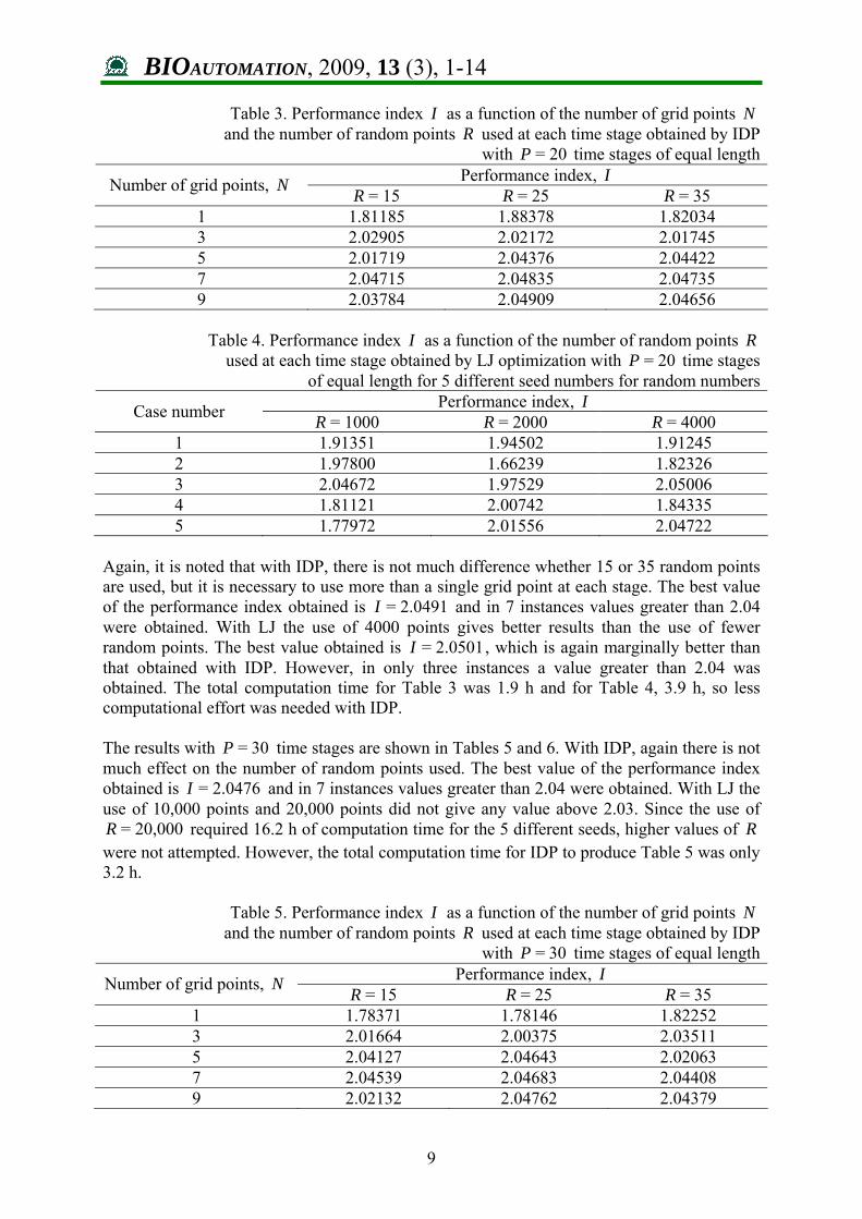
Again, it is noted that with IDP, there is not much difference whether 15 or 35 random points are used, but it is necessary to use more than a single grid point at each stage. The best value of the performance index obtained is 2.0491=I and in 7 instances values greater than 2.04 were obtained. With LJ the use of 4000 points gives better results than the use of fewer random points. The best value obtained is 2.0501=I , which is again marginally better than that obtained with IDP. However, in only three instances a value greater than 2.04 was obtained. The total computation time for Table 3 was 1.9 h and for Table 4, 3.9 h, so less computational effort was needed with IDP. The results with 30=P time stages are shown in Tables 5 and 6. With IDP, again there is not much effect on the number of random points used. The best value of the performance index obtained is 2.0476=I and in 7 instances values greater than 2.04 were obtained. With LJ the use of 10,000 points and 20,000 points did not give any value above 2.03. Since the use of

20,000=R required 16.2 h of computation time for the 5 different seeds, higher values of R were not attempted. However, the total computation time for IDP to produce Table 5 was only 3.2 h.

Table 5. Performance index I as a function of the number of grid points N

and the number of random points R used at each time stage obtained by IDP with 30=P time stages of equal length

Performance index, I Number of grid points, N R = 15 R = 25 R = 35 1 1.78371 1.78146 1.82252 3 2.01664 2.00375 2.03511 5 2.04127 2.04643 2.02063 7 2.04539 2.04683 2.04408 9 2.02132 2.04762 2.04379

BIOAUTOMATION, 2009, 13 (3), 1-14

10

Table 6. Performance index I as a function of the number of random points R used at each time stage obtained by LJ optimization with 30=P time stages

of equal length for 5 different seed numbers for random numbers Performance index, I Case number R = 10000 R = 20000

1 2.02505 2.00530 2 1.86531 1.74982 3 1.95178 1.81786 4 1.97720 1.81047 5 1.97572 1.94522

By using the control policy giving the best result from Table 5, with the corresponding shifting term 0.00436=1 −s as an initial value, a refined run was made with IDP with 25=R . The best value for the performance index 2.05223=I was obtained with P = 30. The optimal control policies are shown in Fig. 1 and Fig. 2, and the corresponding temperature profile is shown in Fig. 3. It is interesting to note the jagged portion of the temperature profile after 0.3=t h. The jags are due to temperature rise during the short time intervals in which the heat generation is kept constant. The best control policy for 30=P and the shifting term were used as initial values for a run with 60=P time stages. The performance index is improved slightly to 2.05243=I . The resulting optimal control policies are shown in Fig. 4 and Fig. 5. The corresponding temperature profile in Fig. 6 shows smaller jags because the time intervals when the heat generation is constant after 0.34=t h are smaller. The use of 120=P time stages yields

2.05253=I and reduces the size of the jags even further as is shown in Fig. 7 and Fig. 8. This value of the performance index is very close to the optimal value 2.0527 reported in the literature [20, 32].

Fig. 1 Optimal feed rate policy with the use

of 30=P time stages of equal length; 2.05223=I

Fig. 2 Optimal heat generation with 30=P

time stages of equal length; 2.05223=I

BIOAUTOMATION, 2009, 13 (3), 1-14

11

Fig. 3 Optimal temperature profile with the use of 30=P time stages of equal

length; 2.05223=I

Fig. 4 Optimal feed rate policy with the use of

60=P time stages of equal length; 2.05243=I

Fig. 5 Optimal heat generation with 60=P

time stages of equal length; 2.05243=I

Fig. 6 Optimal temperature profile with the use of 60=P time stages of equal length;

2.05243=I

BIOAUTOMATION, 2009, 13 (3), 1-14

12

Fig. 7 Optimal heat generation with 120=P

time stages of equal length; 2.05253=I

Fig. 8 Optimal temperature profile with the use of 120=P time stages of equal length;

2.05253=I Conclusions LJ optimization procedure compares very well to IDP in solving the nonisothermal fedbatch optimal control problem. As the number of time stages P is increased, the LJ optimization procedure requires the use of a larger number of random points. However, with IDP the number of random points can be kept small since the search remains in a 2-dimensional space. When the number of time stages is increased to 30, IDP becomes considerably more useful in establishing the optimal control policy. From the jags in the temperature profiles, it is seen that the use of piecewise constant control for heat generation may not be most appropriate, and better results could be obtained by using piecewise linear control for heat generation and piecewise constant control for the feed rate. Since LJ optimization procedure is very easy to program, it is well suited for this type of parametrization. References 1. Bojkov B., R. Hansel, R. Luus (1993). Application of Direct Search Optimization to

Optimal Control Problems, Hungarian J. Industrial Chemistry, 21, 177-185. 2. Fikar M., A. M. Latifi, F. Fournier, Y. Creff (1998). Application of Iterative Dynamic

Programming to Optimal Control of a Distillation Column, Canadian J. Chemical Engineering, 76, 1110-1117.

3. Hartig F., F. J. Keil, R. Luus (1995). Comparison of Optimization Methods for a Fed-batch Reactor, Hungarian J. Industrial Chemistry, 23, 141-148.

4. Hull, T. E., W. D. Enright, K. R. Jackson (1976). User Guide to DVERK − A Subroutine for Solving Nonstiff ODE's, Report 100, Department of Computer Science, University of Toronto, Canada.

5. Liao B., R. Luus (2005). Comparison of the Luus-Jaakola Optimization Procedure and the Genetic Algorithm, Engineering Optimization, 37, 381-398.

BIOAUTOMATION, 2009, 13 (3), 1-14

13

6. Luus R. (1991). Application of Iterative Dynamic Programming to State Constrained Optimal Control Problems, Hungarian J. Industrial Chemistry, 19, 245-254.

7. Luus R. (1993). Optimization of Heat Exchanger Networks, Industrial and Engineering Chemistry Research, 32, 2633-2635.

8. Luus R. (1995). Sensitivity of Control Policy on Yield of a Fed-batch Reactor, Proc. IASTED International Conf. on Modelling and Simulation, Pittsburgh, PA, April 27-29, 224-226.

9. Luus R. (1996). Handling Difficult Equality Constraints in Direct Search Optimization, Hungarian J. Industrial Chemistry, 24, 285-290.

10. Luus R. (1998). Determination of Region Sizes for LJ Optimization Procedure, Hungarian J. Industrial Chemistry, 26, 281-286.

11. Luus R. (1999). Effective Solution Procedure for Systems of Nonlinear Algebraic Equations, Hungarian J. Industrial Chemistry, 27, 307-310.

12. Luus R. (2000). Handling Difficult Equality Constraints in Direct Search Optimization. Part 2, Hungarian J. Industrial Chemistry, 28, 211-215.

13. Luus R. (2000). Iterative Dynamic Programming, Chapman & Hall/CRC. 14. Luus R. (2002). Comparison of LJ Optimization Procedure and IDP in Solving Time

Optimal Control Problems, In: Luus, R. (Ed.), Recent Developments in Optimization and Optimal Control in Chemical Engineering, Research Signpost, Kerela, India, 253-275.

15. Luus R. (2006). Parametrization in Nonlinear Optimal Control Problems, Optimization, 55, 65-89.

16. Luus R. (2007). Use of Line Search in the Luus-Jaakola Optimization Procedure, Proc. Third IASTED International Conf. on Comp. Intelligence, Banff, Alberta, Canada, July 2-4, 128-135.

17. Luus R. (2007). Choosing Grid Points in Solving Singular Optimal Control Problems by Iterative Dynamic Programming, Proc. 10th IASTED International Conf. Intelligent Systems and Control, Cambridge, MA, USA, November 19-21, 425-433.

18. Luus R. (2008). Optimal Control of Oscillatory Systems by Iterative Dynamic Programming, J. Industrial and Management Optimization, 4, 1-15.

19. Luus R. (2009). Direct Search Luus-Jaakola Optimization Procedure, In: Floudas, C. A., P.M. Pardalos (Eds.), Encyclopedia of Optimization, 2nd edition, Springer, 735-739.

20. Luus R. (2009). Handling Inequality Constraints in Optimal Control by Problem Reformulation, Industrial and Engineering Chemistry Research, in press.

21. Luus R. (2009). Formulation and Illustration of Luus-Jaakola Optimization Procedure, In: Rangaiah, G. P. (Ed.), Stochastic Global Optimization: Techniques and Applications in Chemical Engineering, World Scientific, in press.

22. Luus R. (2009). Application of Luus-Jaakola Optimization Procedure to Model Reduction, Parameter Estimation and Optimal Control, In: Rangaiah, G. P. (Ed.), Stochastic Global Optimization: Techniques and Applications in Chemical Engineering, World Scientific, in press.

23. Luus R., M. Galli (1991). Multiplicity of Solutions in Using Dynamic Programming for Optimal Control, Hungarian J. Industrial Chemistry, 19, 55-62.

24. Luus R., D. Hennessy (1999). Optimization of Fed-batch Reactors by the Luus-Jaakola Optimization Procedure, Industrial and Engineering Chemistry Research, 38, 1948-1955.

25. Luus R., T. H. I. Jaakola (1973). Optimization by Direct Search and Systematic Reduction of the Size of Search Region, American Institute of Chemical Engineering J., 19, 760-766.

26. Luus R., W. Mekarapiruk, C. Storey (2001). Evaluation of Penalty Functions for Optimal Control, In: Yang, X, K.L. Teo, and L. Caccetta (Eds.), Optimization Methods and Applications, Kluwer Academic Publishers, 81-103.

BIOAUTOMATION, 2009, 13 (3), 1-14

14

27. Luus R., O. N. Okongwu (1999). Towards Practical Optimal Control of Batch Reactors, Chemical Engineering J., 75,1-9.

28. Luus R., K. Sabaliauskas, I. Harapyn (2006). Handling Inequality Constraints in Direct Search Optimization, Engineering Optimization, 38, 391-405.

29. Luus R., C. Storey (1997). Optimal Control of Final State Constrained Systems, In: Proc. IASTED Int. Conf. Modeling, Simulation and Optimization, Singapore, August 11-13, 245-249.

30. Mekarapiruk W., R. Luus (1997). Optimal Control of Inequality State Constrained Systems, Industrial and Engineering Chemistry Research, 36, 1686-1694.

31. Rusnak A., M. Fikar, M. A. Latifi, A. Meszaros (2001) Receding Horizon Iterative Dynamic Programming with Discrete Time Models, Computers and Chemical Engineering, 25, 161-167.

32. Schlegel M., W. Marquardt (2006). Detection and Exploitation of the Control Switching Structure in the Solution of Dynamic Optimization Problems, J. Process Control, 16, 275-290.

33. Srinivasan B., S. Palanki, D. Bonvin (2003). Dynamic Optimization of Batch Processes I. Characterization of the Nominal Solution, Computers and Chemical Engineering, 27, 1-26.

34. Stoyanov S. (2009). Analyses of Methods and Algorithms for Modelling and Optimization of Biotechnological Processes, Bioautomation, 13, 1-18.

Prof. Rein Luus, Ph.D., P.Eng.

e-mail: rein.luus@utoronto.ca

Rein Luus received Ph.D. degree in chemical engineering in 1964 and was offered the Sloan postdoctoral fellowship at Princeton University. In 1965 he started work in the Department of Chemical Engineering at University of Toronto, becoming Assistant Professor, Associate Professor in 1968, Professor in 1973 and Professor Emeritus since 2005. He is laureate of the Steacie Prize (1976), the ERCO Award in Chemical Engineering (1980) and other awards for his teaching competencies. He has served as a consultant for Canadian General Electric, Shell Canada, Milltronics, Imperial Oil, and Fiberglas. For 42

years he has guided about 20 master students and 10 Ph.D. students. He has published about 200 papers in scientific journals and refereed conference proceedings, five articles in the Encyclopedia of Optimization (Springer, 2009), and chapters in several books on optimization. He has developed several methods and algorithms for global optimization, as the well-known Luus – Jaakola (LJ) and Wang – Luus (WL) methods. Research interests: optimization, optimal process control, iterative dynamic programming, mathematical modeling, parameter estimation, model reduction, optimal control of oscillatory systems, stability and nonlinear analysis.