Supervisor: Martin Holmén Master Degree Project No. 2014:94 Graduate School

Master Degree Project in Finance

Investors’ Pursuit of Positive Skewness in Stock Returns An empirical study of the Skewness effect on market-to-book ratio

Amir Omed and Jiayin Song

Investors’ Pursuit of Positive Skewness in Stock Returns

- An Empirical Study of the Skewness Effect on Market-to-Book Ratio

Amir Omed and Jiayin Song1

School of Business, Economics and Law, University of Gothenburg

Master of Science in Finance – Spring 2014

Abstract

This paper finds that higher positive skewness in stocks’ return distribution may lead

to higher valuation in terms of market-to-book ratio. In addition, we find that this

relationship was not affected by the recent financial crisis in 2008. These inferences

remain qualitatively unchanged subject to robustness testing. We propose well-known

psychological biases as partial reasons for investors’ preference for positive skewness.

1 The authors would like to thank supervisor Martin Holmén for his inspiration and constructive criticism.

Table of Contents

1. INTRODUCTION 1

2. THEORY AND LITERATURE REVIEW 2

3. METHOD 3

3.1. HYPOTHESES DEVELOPMENT AND RESEARCH DESIGN 4 3.2. CHOSEN PRE- AND POST-CRISIS PERIOD 4 3.3. SAMPLE DESCRIPTION 5 3.4. DATA MANAGEMENT FOR DESCRIPTIVE STATISTICS 6 3.5. VARIABLES OF INTEREST 6 3.6. TEST FOR ROBUSTNESS 8

4. RESULTS 9

4.1. DESCRIPTIVE STATISTICS 9 FULL SAMPLE PERIOD 9 PRE- AND POST-CRISIS PERIOD 11 4.2. CROSS-SECTIONAL RESULTS 12 THE EFFECT OF EX ANTE SKEWNESS ON MARKET-TO-BOOK RATIO 12 SKEWNESS COEFFICIENT STABILITY FOR THE PRE- AND POST-CRISIS PERIODS 12 ROBUSTNESS 14 SUPPLEMENTARY FINDINGS 17

5. DISCUSSION 18

5.1. PREFERENCE FOR SKEWNESS 18 5.2. DESIRE FOR UPSIDE POTENTIAL 18 5.3. BEARING ADDITIONAL VOLATILITY 19 5.4. PSYCHOLOGICAL BIASES 19 5.5. THE RECENT FINANCIAL CRISIS 20

6. CONCLUSION 21

REFERENCES 22

APPENDIX 25

SPEARMAN CORRELATION ANALYSIS 25 SENSITIVITY ANALYSIS 26 TIME PERIOD TEST 26 CONTROL VARIABLE TEST 27 OTHER SENSITIVITY TESTS 29 WINSORIZATION 31

1

1. Introduction

The skewness in stocks’ return distribution, defined as the third moment of returns, quantifies to

what extent the distribution is asymmetric – compared to a normal distribution that is symmetric with

zero skewness. Positive skewness is intuitively thought of as a distribution with a longer right tail

with higher probability for extremely high gains. In contrast, negative skewness is a distribution with

a longer left tail with higher probability for extremely high losses.

In this paper, we conduct an empirical study on the impact of skewness in stocks’ return distributions

on their market-to-book ratios. In particular, we contribute to the existing literature by demonstrating

an important link between skewness preference and higher market price relative to firms’

fundamentals. Our results suggest that higher positive skewness may lead to higher market-to-book

valuation.

In addition, we compare two periods for a possible change in this relationship; the pre-crisis of 2008

versus the post-crisis period. Barone-Adesi et al. (2013) find that excessive optimism and

overconfidence are positively correlated, and therefore inflating asset prices in good times and

intensifying market crashes in bad times. They find that when these biases are strong, investors

believe that risk and return are negatively correlated. The 2008 crisis was a powerful chock to the

financial system and the real economy in many senses. It is therefore of high interest to investigate

any possible changes in investor preference after such a disruption. We further contribute to the

existing literature by investigating changes in preference for skewness after the financial crisis. We

find no evidence that would suggest any changes in the higher valuation investors apply to stocks

with positive skewness after the financial crisis of 2008. The results for our study remain

qualitatively unchanged after robustness testing. Although the financial system and the real economy

received a powerful shock, together with huge investor losses, the memory seems to be short.

Investors continue to pursue high gains with small probabilities by applying a premium to stocks

possessing these attributes.

We use our empirical results and earlier behavioral finance literature to present possible reasons for

the preference for skewness among investors and the higher valuation applied to stocks with these

attributes.

2

2. Theory and Literature Review

Prior literature suggests that investors prefer positively skewed stocks and thus apply a higher

valuation to them in terms of higher market-to-book ratios (glamour stocks2) than negatively, or less

positively, skewed stocks with lower market-to-book ratios (value stocks) (Zhang, 2013).

In particular, Zhang (2013) finds that the premium (discount) investors apply to glamour (value)

stocks is significantly correlated with the difference in return skewness. Zhang’s finding suggests a

partial explanation to the value/glamour-stock puzzle. This phenomenon, sometimes referred to as

the value/glamour anomaly, proposes that value stocks tend to outperform glamour stocks (Basu,

1977; Rosenberg et al., 1985; Fama and French, 1992). These findings challenge the predictions of

the efficient market hypothesis and the capital asset pricing model of Sharpe (1964) and Lintner

(1965). Earlier research try to explain this anomaly and conclude that investor mispricing plays a

major role (Lakonishok et al., 1994; La Porta, 1996; Piotroski, 2000), and that this correlation

between value stocks and its outperformance may be spurious (Kothari et al., 1995; Chan et al.,

1995), but can also have a partial explanation of investors bearing higher risk and transaction costs,

and thus be compensated for it (Fama and French, 1995; Berk et al., 1999; Zhang, 2005; Xing, 2008;

Penman and Reggiani, 2012).

The effect of skewness on asset pricing has been a topic for researchers for decades. 3 The

conventional asset pricing models, such as the capital asset pricing model, are one of the main

reasons to why this is a hot topic. These conventional models make no predictions of skewness effect

on asset pricing. Earlier papers investigate this matter and find that coskewness, defined as the

movement of stock return skewness with the skewness of a well-diversified asset portfolio, has an

impact on asset pricing, albeit with mixed results (Friend and Westerfield, 1980; Harvey and

Siddique, 2000; Hung et al., 2004; Post et al., 2008).

In the area of behavioral finance linked to investor preference for positively skewed stocks, Barberis

and Huang (2008) analyze an equilibrium asset pricing model based on the cumulative prospect

theory from Kahneman and Tversky (1992). They conclude that in their equilibrium model,

idiosyncratic stock return skewness is priced. More positively skewed stocks earn lower average

returns, all else held constant. Similarly, Mitton and Vorkink (2007) develop a one-period model of

2 The notation ”glamour” is widely used in academic literature to describe stocks with higher valuation. It is also sometimes referred to as ”growth” stocks. A “value” stock refers to stocks with lower valuation. 3 Research on skewness dates back at least to Rubinstein (1973) and Kraus and Litzenberger (1976, 1983).

3

investor asset holdings where investors have heterogeneous preference for skewness and find that the

apparent mean-variance inefficiency of underdiversified investors can be largely explained by the

fact that investors sacrifice mean-variance efficiency for higher skewness exposure. Brunnermeier et

al. (2007) argue that investor preference for positively skewed stocks can be explained by that

humans want to believe in what makes them happy and want to make good decisions that may lead

to good outcomes in the future. Brunnermeier et al. (2007) argue further that investors care about

expected future utility flows and are therefore happier if they overestimate the probabilities of such

states in which their investments pay off well – even though such optimism would lead to suboptimal

decision-making and lower levels of utility on average ex post. Earlier research also links the

observed investor preference for positively skewed stocks to lotteries, which is highly positively

skewed, and to betting on races where long-shots have lower expected returns than favorites (Zhang

2005).

Most recently in the investigation of correlation between higher moments and asset pricing is from

Zhang (2013) who provides an alternative view in a risk-reward analysis by also investigating the

skewness of stock returns. Earlier research is conducted on the correlation between skewness and

returns, as well as between coskewness and returns, but with the market-to-book ratio as a control

variable. The effect of market-to-book ratio is fixed to determine the impact of skewness on returns.

Zhang (2013) takes it one step further and examines the effect of skewness on market-to-book ratio

and concludes that it indeed exists a significant correlation between these two.

3. Method

Our paper expands on Zhang (2013) and first examines the relationship between market-to-book

ratio and skewness, and in addition test whether this relationship has changed between two periods;

2003-2007 and 2008-2012 – the pre- and post-crisis.4 We begin with investigating whether investors

apply a higher market-to-book ratio on positively skewed stocks. A comparison is then made

between the pre- and post-crisis to see if this behavior has changed. Defining an exact date for when

the crisis started is ambiguous, but as we use a total of ten-year period we believe that the bias, if

such exists, will be small. Despite this belief, we perform a sensitivity analysis with different time

periods to investigate whether the results change. Previous research has been conducted on firms

listed in the U.S, while our data is from firms listed in Sweden. Albeit a larger universe of stocks is

4 Refer to our argument for this chosen period under the “Chosen Pre- and Post-Crisis” subsection.

4

available in the U.S., we choose to focus on our home market, which has a sufficiently large sample.

We estimate cross-sectional time series regression, i.e. panel data, with fixed effects.5

3.1. Hypotheses Development and Research Design

We establish two hypotheses to base our research design on. The first refers to the overall

relationship between market-to-book ratio and skewness, and the second to the comparison between

the pre- and post-crisis periods.

H1: Stocks with high positive skewness in their return distributions have a higher market-to-book

ratio compared to stocks with a lower skewness.

If investors have preference for positively skewed stocks and thus apply a higher valuation to them,

investors could use this information as part of their decision-making when investing. Any useful

information in investing behavior and preference could improve return predictability and perhaps

shed light on the relationship between return and higher moment risks.

H2: The 2008 financial crisis did have a significant impact, positively or negatively, on the

relationship between skewness of stocks’ return distribution and their market-to-book ratios.

Any disruption between a possible relationship between skewness and market-to-book ratio would

provide valuable knowledge of future crisis’ impact on investing behavior. Barone-Adesi et al.

(2013) find that excessive optimism and overconfidence are positively correlated, and therefore

inflating asset prices in good times and intensifying market crashes in bad times. In addition, they

find that when these biases are strong, investors believe that risk and return are negatively correlated.

By examining this relationship, we may be able to conclude if investors have a short memory of bad

‘episodes’ and if the memory of the 2008 shock has been forgotten or diminished in terms of

preferences for skewness.

3.2. Chosen Pre- and Post-Crisis Period

To determine an exact date for when the financial crisis started is somewhat ambiguous. On 9 August

2007, BNP Paribas announced that it was ceasing activity in three hedge funds that specialized in US

mortgage debt. This moment was one of the first eye openers to the fact that there were tens of

5 Fixed effects regression is used when controlling for omitted variables that may differ between entities, in our case firms, but are constant over time. With help of these fixed effects, we can estimate the changes in the coefficients of our independent variables over time. (Greene, 2011)

5

trillions of dollars worth of derivatives with a doubtful current market value. This led to a domino

effect of banks and investors being more restrictive in their actions. It was not until Lehman Brothers

was allowed to go bankrupt by the U.S. government on 15 September 2008 that the stock markets

reacted rapidly6. Based on these events, we choose the start of the post-crisis period as 1 January

2008 to 31 December 2012, and the pre-crisis as 1 January 2003 to 31 December 2007. However, we

perform a sensitivity analysis for two additional time periods to mitigate any possible time period

bias. The alternative time periods are 2003-2008 versus 2009-2012, and 2003-2006 versus 2007-

2012.

3.3. Sample Description

The data is from Bloomberg and is based on 233 stocks that are or have been listed on the NASDAQ

OMX Stockholm Exchange7 for at least two years at any time during the period 1 January 2003 to 31

December 2012. We include 50 stocks that have been delisted due to various reasons, such as buy-

outs and bankruptcies, in order to mitigate a possible survivorship bias.

We arrange a list of requirements for the firms that need to be fulfilled in order to clean the data

before running any tests. Our first requirement is that the firms must have a calendar year as fiscal

year, i.e. year-end report at 31 December. All other firms are excluded. Next, we drop firms with

negative shareholder’s equity, i.e. book value, since such a company, theoretically, would be

bankrupt, and thus not have any obvious interpretation (Brown et al. 2007). This would also lead to a

negative market-to-book ratio. An alternative approach would be to only drop the negative

observations and not the entire firm. However, this would lead to the question; what do we replace

the negative value with? If last known positive value would be used, the data would be tweaked and

a potential upward bias would occur. Next requirement is that we only keep non-financial firms

motivated by the financial sector’s accounting standards and high leverage, which cannot be

compared to non-financial firms. Next, we only include one of the stock’s share class; e.g. for Volvo

A and B; we use the most liquid share class, which is often the class B share with some exemptions.

Lastly, we correct for outliers by winsorizing at the top and bottom 5%.8

6 See for instance “Global Financial Crisis: five key stages 2007-2011” by Larry Elliott (2012), editor at The Guardian. 7 The stocks covered are listed on the Small, Mid and Large Cap lists. 8 Note that this is not equivalent to simply excluding the outliers; instead we replace the extreme values with the values closest to them. We do not winsorize stock returns, as this would hugely impact our research on skewness.

6

3.4. Data Management for Descriptive Statistics

In this part, we separate the stocks into three groups and present descriptive statistics for skewness,

kurtosis and volatility for the three groups. We sort the market-to-book ratio of all stocks from

highest to lowest. Firms in the top three deciles are classified as “High M-B”, while firms in the

bottom three deciles are classified as “Low M-B”, and with the remaining placed into “Median M-

B”. Descriptive statistics are based on daily excess returns defined as raw return less market index

OMXSPI return. The purpose of using excess return instead of raw return for the descriptive

statistics is to control for the influence of volatility. Zhang (2013) calculates excess return with two

different methods. The first approach is based on raw return less market index return and the second

one as beta-adjusted return. The results remain qualitatively unchanged.

3.5. Variables of Interest

We define “M-B” as the market-to-book ratio and use it as our dependent variable. We follow

Zhang’s (2013) approach with a discrepancy between the date for book value and market value. We

retrieve book values from 31 December Y1 and market value from the last trading day of April in

Y2. The reason for this discrepancy is due to incorporation of information of the book value of

31 December, i.e. the release of their financial reports can take up to four months. Furthermore, we

cannot use companies that do not have calendar year as fiscal year.9 “SIZE” is the natural logarithm

of sales for calendar year Y1. “LEV” is the Company’s leverage ratio defined as debt-to-total assets

where we use values from 31 December Y1 – consistent with “SIZE. “MOM” is the momentum

effect, the last twelve months’ yearly return preceding the last trading day of April Y2. This variable

is included since it may be correlated with the skewness and kurtosis (see for instance Chang,

Christoffersen and Jacobs 2009; Fama and French 1993). “Ex ante SKEW” is the daily stock return’s

skewness, the third moment of returns, for the preceding twelve months before last trading day of

April Y2. The following formula is used for calculating skewness

𝑆𝑘𝑒𝑤𝑛𝑒𝑠𝑠 = 𝑛 ∑ (𝑥𝑖 − �̄�)3𝑛

𝑖=1

�(𝑛 − 1)(𝑛 − 2)�𝑠3

9 Assume Company A has fiscal year-end at 30 August. If we use market value for four months after this date, i.e. 31 January the following year, we use market value at different dates for the different companies. This would lead to inconsistent measurement of our data points. The alternative would be to use the market value from 30 April, i.e. consistent market value dates, but would have the issue of the following quarterly report after 30 August already being published, which would result in the market value incorporating a later known book value than our data point. Thus, we need to exclude companies with non-calendar years as fiscal years.

7

where 𝑥𝑖 is the daily stock return, �̄� is the sample mean, 𝑛 is the number of observations, and 𝑠 is the

sample standard deviation. “Ex post SKEW” is the following twelve months after the last trading day

of April in Y2. We assume that investors’ skewness expectation is unbiased, such that the actual ex

post return skewness approximates the expected return skewness in our sample, on average. Actual

skewness at t+1 is approximately equal to average expected skewness at time t (Zhang 2013). The

same assumption is made for “Ex post STDV” and “Ex post KURT”. “Ex ante STDV” is the stock

return’s standard deviation, commonly referred to as volatility or the second moment of returns, for

the preceding twelve months before the last trading day of April in Y2. The following formula is

used for calculating standard deviation

𝑆𝑡𝑎𝑛𝑑𝑎𝑟𝑑 𝐷𝑒𝑣𝑖𝑎𝑡𝑖𝑜𝑛 = �∑ (𝑥𝑖 − �̄�)2𝑛𝑖=1

(𝑛 − 1)

where 𝑥𝑖 is the daily stock return, �̄� is the sample mean and 𝑛 is the number of observations. “Ex

post STDV” is the stock return’s standard deviation for the following twelve months after the last

trading day of April in Y2. “Ex ante KURT” is the stock return’s kurtosis10, the fourth moment of

returns, for the preceding twelve months before the last trading day of April in Y2. The following

formula is used for calculating kurtosis

𝐾𝑢𝑟𝑡𝑜𝑠𝑖𝑠 =𝑛(𝑛 + 1)

(𝑛 − 1)(𝑛 − 2)(𝑛 − 3)∑ (𝑥𝑖 − �̄�)4𝑛𝑖=1

𝑠4−

3(𝑛 − 1)2

(𝑛 − 2)(𝑛 − 3)

where 𝑥𝑖 is the daily stock return, �̄� is the sample mean, 𝑛 is the number of observations, and 𝑠 is the

sample standard deviation. “Ex post KURT” is the stock return’s kurtosis for the following twelve

months after the last trading day of April in Y2. In addition, standard deviation, skewness and

kurtosis are also calculated based on excess return – defined as raw daily return less market index

OMSPI daily return. These variables are denoted as its original name plus E in the end, e.g. “Ex ante

SKEW_E”. Where lags are used, we denote those variables with “L1” in the beginning of the

variable name for lag one. “GSALES” is the growth rate in sales for calendar year Y1 over Y0. To

summarize, our main model will be conducted as follows.

𝑀𝐵𝑖,𝑡 = 𝛽0 + 𝛽1𝑆𝐼𝑍𝐸𝑖,𝑡 + 𝛽2𝐿𝐸𝑉𝑖,𝑡 + 𝛽3𝐸𝑥 𝐴𝑛𝑡𝑒 𝑆𝐾𝐸𝑊𝑖,𝑡 + 𝛽4𝐸𝑥 𝐴𝑛𝑡𝑒 𝐾𝑈𝑅𝑇𝑖,𝑡 + 𝛽5𝐸𝑥 𝐴𝑛𝑡𝑒 𝑆𝑇𝐷𝑉𝑖,𝑡 + 𝜀𝑖,𝑡

10 Kurtosis is a measure of whether the data is peaked or flat relative to a normal distribution. Datasets with high kurtosis tend to have a sharp peak and decline quickly. Low kurtosis datasets have a flat top and decline more slowly.

8

where 𝑀𝐵𝑖,𝑡 is the market-to-book ratio for observation i=1,…,n, and time t=2003,…,2012. SIZE is

the log of total sales, LEV is debt-to-total assets, Ex Ante SKEW, KURT and STDV are the

skewness, kurtosis and standard deviation for the last twelve months return. 𝜀𝑖,𝑡 is the error term.

3.6. Test for Robustness

A Hausman specification test is conducted for our cross-sectional regression to choose between

random and fixed effects (Hausman, 1978). This test evaluates the significance of an estimator of

fixed effects versus an estimator of random effects. Moreover, we test for heteroskedasticity in our

panel data with a two-step Generalized Least Squares (GLS) estimation. The first step includes one

model that corrects for heteroskedasticity and one that does not. These two estimators are tested

against each other with the Likelihood ratio. We investigate serial correlation in our panel data model

with the help of a Wooldridge (2002) test. We correct for serial correlation in one model but not for

heteroskedasticity to compare the results with our main model with heteroskedasticity-consistent

standard errors. In all other models throughout this report, we use heteroskedasticity-consistent

standard errors. To continue our analysis of serial correlation, we add the first lag of Ex ante SKEW,

namely L1.Ex ante SKEW, combined with Ex ante SKEW, KURT and STDV. To further test these

lags, we replace Ex ante SKEW, KURT and STDV with only their first lags.

Additionally, we only use Ex post values in a separate model; Ex post SKEW, KURT and STDV. Ex

post is equivalent to the lead of Ex ante. The fit of the models is tested with Bayesian Information

Criteria (BIC). The investigation of serial correlation is finalized by adding the first lag of the

dependent variable M-B to one of our models.

In the presence of possible multicollinearity, the estimators are still Best Linear Unbiased Estimators

(BLUE), but the variance could be inflated. We investigate any severe multicollinearity with a

simple correlation matrix.

Spurious correlation will affect our results when SIZE is defined as the market capitalization as this

variable is the numerator of our dependent variable, M-B. Any relationship will merely be a

mechanical correlation without any useful interpretation and thus makes the results biased.

Additionally, defining leverage as debt-to-equity results in a similar issue with equity, which is the

denominator of M-B. These issues are diminished by defining SIZE as log of total sales and by

defining LEV as debt-to-total assets. However, regarding LEV, we exclude it in one model to see if

leverage has a strong impact on the coefficient of skewness.

9

Regarding the intercept in our regression models, it should not be interpreted in any useful manner as

we run a fixed effects model. The intercept is arbitrarily chosen by STATA and works only as a

constraint on the fixed effects system. Consequently, we choose to omit them from our output tables.

To compare the two periods’ skewness coefficient, and to see if these two coefficients differ

significantly from each other, we perform a Chow test, a parameter instability test. This test is

repeated using two alternative time period breaks.11

Lastly, the most crucial assumption of regression models is discussed – namely the correlation

between the regressors and the error term and thus a potential omitted variable bias. A violation of

this assumption would bias our results considerably. To prove this assumption is difficult, if not

impossible in most cases. A common and popular approach is to use fixed effects. The positive

aspect of using fixed effects is that it controls for omitted variables that do not change over time. The

negative aspect is that it reduces possible important signal from the data.

4. Results

4.1. Descriptive Statistics

Full Sample Period

An average M-B ratio of 4.89 is found for “High M-B”, 2.47 for “Median M-B”, and 1.27 for “Low

M-B”. The groups’ respective skewness statistics based on excess return are reported in Table I.

Table I: Descriptive Statistics of Skewness for Each M-B Group

Full Sample Period – 2003-2012

N Mean Median Std. Dev.

Low M-B 70 0.358 0.287 0.410

Median M-B 92 0.536 0.439 0.472

High M-B 70 0.558 0.446 0.498 Table I: This table reports descriptive statistics; mean, median and standard deviation for skewness based on excess return, for the full sample period 2003-2012. “Low M-B” consists of the bottom three deciles of the stocks’ market-to-book ratios. “High

M-B” consists of the top three deciles, and the remaining four deciles are placed in “Median M-B”.

11First alternative time periods are 2003-2008 vs. 2009-2012 and the second one being 2003-2006 vs. 2007-2012 used as part of our sensitivity analysis. We use 2003-2007 vs. 2008-2012 as main time periods throughout our report.

10

Stocks with higher market-to-book ratios have a higher skewness compared to stocks with lower

market-to-book ratios. The skewness difference is more distinctive between “Low M-B” and “High

M-B”. The sample median and mean differs noticeably due to high extreme values shifting the mean.

Table II: Pearson Correlation Matrix Based On Excess Return M-B Ex ante

SKEW_E Ex ante

KURT_E Ex ante

STDV_E Ex ante SKEW_E 0.19*** - - -

Ex ante KURT_E 0.14*** 0.41*** - -

Ex ante STDV_E 0.01 0.34*** 0.35*** -

Table II: This table reports Pearson correlation coefficient estimations for the full sample period. “_E” denotes that the variables are based on excess return. ***, ** and * show significance levels for p<0.01, p<0.05 and

p<0.1, respectively.

To further test the relationship between market-to-book ratio and skewness, Pearson12 correlation

coefficients are presented (Table II). The coefficient between skewness and market-to-book is 0.19

and significant at a one per cent significance level.

Graph I shows a simple linear prediction of skewness on market-to-book ratio with 95% confidence

interval. An apparent positive slope exists between these two variables - higher skewness is

positively correlated with higher market-to-book ratio.

Graph I: Linear Prediction with Skewness on Market-to-Book Ratio

Graph I: Linear prediction of skewness on market-to-book ratio with confidence interval plots. Skewness is based on

excess return.

12 Spearman correlation matrix has been conducted as well; please see Appendix, Table X.

11

Pre- and Post-Crisis Period

To test the consistency of the relationship between skewness and market-to-book before and after the

financial crisis, we examine this relationship between two periods, 2003-2007 and 2008-2012. The

significance of correlation remains and linear prediction generates similar results.

Table III: Descriptive Statistics of Skewness for Each M-B Group

Pre-Crisis Period – 2003-2007

N Mean Median Std. Dev.

Low M-B 53 0.387 0.296 0.494

Median M-B 79 0.584 0.493 0.533

High M-B 55 0.658 0.543 0.613 Table III: This table reports descriptive statistics; mean, median and standard deviation for skewness based on excess return,

for the pre-crisis period 2003-2007. “Low M-B” consists of the bottom three deciles of the stocks’ market-to-book ratios. “High M-B” consists of the top three deciles, and the remaining four deciles are placed in “Median M-B”.

The pre-crisis period shows a similar pattern of relationship between the three groups. However, the

difference in skewness between “Low M-B” and “High M-B” is more noticeable for the pre-crisis

period compared to the full period presented earlier. For the “High M-B” group in the full period,

median skewness value is 0.446 compared to the corresponding number of 0.543 for the pre-crisis

period. The “Low M-B” group has a median value of 0.287 and 0.296 for the full sample period and

the pre-crisis period, respectively.

Table IV: Descriptive Statistics of Skewness for Each M-B Group

Post-Crisis Period – 2008-2012

N Mean Median Std. Dev.

Low M-B 70 0.338 0.294 0.504

Median M-B 87 0.537 0.463 0.517

High M-B 64 0.510 0.362 0.613 Table IV: This table reports descriptive statistics; mean, median and standard deviation for skewness based on excess return, for the post-crisis period 2008-2012. “Low M-B” consists of the bottom three deciles of the stocks’ market-to-book ratios.

“High M-B” consists of the top three deciles, and the remaining four deciles are placed in “Median M-B”.

The post-crisis period shows a disconnection in the pattern for the three groups. The median

skewness value for “High M-B” is lower than “Median M-B”. Their difference is diminished if

12

comparing mean values. The “High M-B”, “Median M-B” and “Low M-B” show median skewness

values of 0.362, 0.463 and 0.294, respectively. This pattern disconnection is not consistent with

neither the full sample period nor the pre-crisis period, nor is it consistent with Zhang’s (2013)

empirical findings. The median skewness for “High M-B” in the post-crisis period, 0.362, is

considerably lower than the corresponding number for the pre-crisis period, 0.543. During and after

the crisis, the positive skewness decreased most noticeably for higher valued stocks – there were less

extreme high gains in this group.

4.2. Cross-Sectional Results

Results reported under the “Descriptive Statistics” section indicate that firms with different market-

to-book ratios have different skewness in their stock returns. In particular, higher positive skewness

is associated with higher market-to-book ratio. In this part, we focus on examining if skewness has

an effect on market-to-book ratio and control for a set of variables of interest.

The Effect of Ex Ante Skewness on Market-to-Book Ratio

Our main model is regressed on market-to-book ratio (M-B), with log of sales (SIZE) debt-to-total

assets (LEV) and last twelve months skewness, kurtosis and standard deviation based on raw returns

(Ex ante SKEW, Ex ante KURT and Ex ante STDV, respectively) as independent variables using

fixed effects panel data model.

All variables show significant results at the one per cent significance level, with the exception of

kurtosis, presented under Table V. Skewness shows a positive significant coefficient of 0.26 for the

full period. Higher skewness leads to higher market-to-book. This is consistent with our first

hypothesis.

Skewness Coefficient Stability for the Pre- and Post-Crisis Periods

Table V shows a difference in the skewness coefficient between the pre- and post-crisis with a

coefficient of 0.31 and 0.27, respectively. Results show a significant skewness coefficient at the one

per cent level for all three periods; pre-, post and full period. The coefficients for standard deviation

and leverage are significant at the one per cent significance level for all three periods. The log of

sales shows an insignificant and positive coefficient for the pre-crisis period, which is in

contradiction with the full sample period and the post-period, and with a considerably higher

standard error of 0.26.

13

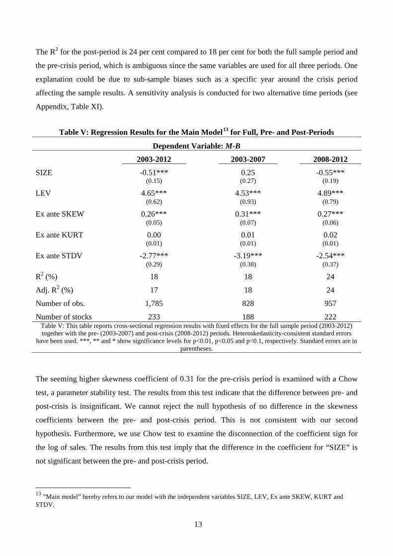
The R2 for the post-period is 24 per cent compared to 18 per cent for both the full sample period and

the pre-crisis period, which is ambiguous since the same variables are used for all three periods. One

explanation could be due to sub-sample biases such as a specific year around the crisis period

affecting the sample results. A sensitivity analysis is conducted for two alternative time periods (see

Appendix, Table XI).

Table V: Regression Results for the Main Model13 for Full, Pre- and Post-Periods

Dependent Variable: M-B

2003-2012 2003-2007 2008-2012

SIZE -0.51*** 0.25 -0.55*** (0.15) (0.27) (0.19)

LEV 4.65*** 4.53*** 4.89*** (0.62) (0.93) (0.79)

Ex ante SKEW 0.26*** 0.31*** 0.27*** (0.05) (0.07) (0.06)

Ex ante KURT 0.00 0.01 0.02 (0.01) (0.01) (0.01)

Ex ante STDV -2.77*** -3.19*** -2.54*** (0.29) (0.38) (0.37)

R2 (%) 18 18 24

Adj. R2 (%) 17 18 24

Number of obs. 1,785 828 957

Number of stocks 233 188 222 Table V: This table reports cross-sectional regression results with fixed effects for the full sample period (2003-2012) together with the pre- (2003-2007) and post-crisis (2008-2012) periods. Heteroskedasticity-consistent standard errors

have been used. ***, ** and * show significance levels for p<0.01, p<0.05 and p<0.1, respectively. Standard errors are in parentheses.

The seeming higher skewness coefficient of 0.31 for the pre-crisis period is examined with a Chow

test, a parameter stability test. The results from this test indicate that the difference between pre- and

post-crisis is insignificant. We cannot reject the null hypothesis of no difference in the skewness

coefficients between the pre- and post-crisis period. This is not consistent with our second

hypothesis. Furthermore, we use Chow test to examine the disconnection of the coefficient sign for

the log of sales. The results from this test imply that the difference in the coefficient for “SIZE” is

not significant between the pre- and post-crisis period.

13 ”Main model” hereby refers to our model with the independent variables SIZE, LEV, Ex ante SKEW, KURT and STDV.

14

Robustness

The Hausman specification test suggests that fixed effects best suits our model compared to random

effects.

The two-step GLS heteroskedasticity test shows that there is presence of heteroskedasticity in our

panel data, which is why we use heteroskedasticity-consistent standard errors across all models. The

results from the Wooldridge test indicate the presence of serial correlation in our main model. A

correction was made for this serial correlation but the results remain identical compared to our main

model with heteroskedasticity-consistent standard errors. This implies that running our model with

heteroskedasticity-consistent standard errors in a fixed effects model corrects for serial correlation as

well as heteroskedasticity. The remaining models use heteroskedasticity-consistent standard errors.

Table VI: Regression Results including Lags Dependent Variable: M-B

Model I Model II Model III

SIZE -0.51*** -0.62*** -0.68*** (0.15) (0.16) (0.13)

LEV 4.65*** 4.64*** 4.05*** (0.62) (0.71) (0.64)

Ex ante SKEW 0.26*** 0.24*** 0.31*** (0.50) (0.50) (0.50)

Ex ante KURT 0.00 0.00 0.00 (0.01) (0.01) (0.01)

Ex ante STDV -2.77*** -1.93*** -1.80*** (0.29) (0.33) (0.32)

L1.Ex ante SKEW 0.12** (0.05)

L1.M-B 0.29*** (0.04)

R2 (%) 18 16 25 Adj. R2 (%) 17 15 24 Number of obs. 1,785 1,552 1,554 Number of stocks 233 226 226

Table VI: This table reports cross-sectional regression results with fixed effects for the full sample period 2003-2012. “L1.” denotes the first lag of the variable. Model I is our main model. Model II has the first lag of

Ex ante SKEW included. Model III has the first lag of the dependent variable M-B included. Heteroskedasticity-consistent standard errors have been used. ***, ** and * show significance levels for

p<0.01, p<0.05 and p<0.1, respectively. Standard errors are in parentheses.

15

Including the skewness lag does not change the qualitative results with the significant positive

coefficient intact (Table VI, model II). When adding the first lag of the dependent variable M-B, the

qualitative results do not change (Table VI, model III).

Table VII: Regression Results Including Lags Dependent Variable: M-B Model I Model II SIZE -0.51*** -0.60***

(0.15) (0.13)

LEV 4.65*** 4.15*** (0.62) (0.66)

Ex ante SKEW 0.26*** (0.05)

Ex ante KURT 0.00 (0.01)

Ex ante STDV -2.77*** (0.29)

L1.Ex ante SKEW 0.10* (0.05)

L1.Ex ante KURT 0.00 (0.01)

L1.Ex ante STDV -0.37 (0.30)

R2 (%) 18 12 Adj. R2 (%) 17 12 Number of obs. 1,785 1,564 Number of stocks 233 227

Table VII: This table reports cross-sectional regression results with fixed effects. Model I is our main model. Model II replaces ex ante values with the first lag of it - denoted with “L1.”. Heteroskedasticity-

consistent standard errors have been used. ***, ** and * show significance levels for p<0.01, p<0.05 and p<0.1, respectively. Standard errors are in parentheses.

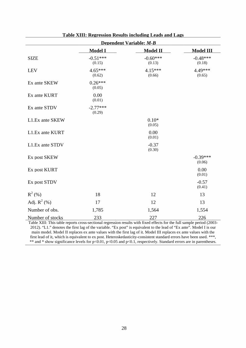
When only lags are included, replacing the ex ante values, the coefficient of skewness is significant

and positive at a ten per cent significance level (Table VII, model II). However, when only post

values are used, the coefficient of skewness is negative and significant at a one per cent significance

level, which contradicts earlier research (Zhang, 2013) (Appendix, Table XIII, model III). This

inconsistency could be due to the reason that investors’ expected skewness is not equal to actual

skewness for the following twelve months, i.e. Ex post SKEW. Investors may have difficulties to

forecast skewness, which supports the positive coefficients of Ex ante SKEW and its first lag. As Ex

ante SKEW and the first lag are historical, investors are aware of it. However, for Ex post SKEW, it

16

is an assumption of investors’ expected skewness being equal to actual Ex post SKEW. Our

conclusion is that Ex post SKEW serves as a poor indicator for the relationship between

contemporaneous skewness and market-to-book ratio.

The two models (Table VII, model I and II) are concluded with the Bayesian Information Criteria,

which suggests that using only Ex ante values fits the data better (Model I).

Table VIII: Pearson14 Correlation Matrix Based on Raw Returns M-B SIZE LEV Ex ante

SKEW Ex ante KURT

Ex ante STDV

MOM

SIZE -0.16*** - - - - - - LEV -0.05* 0.47*** - - - - - Ex ante SKEW 0.15*** -0.37*** -0.18*** - - - - Ex ante KURT 0.12*** -0.29*** -0.11*** 0.50*** - - - Ex ante STDV 0.02 -0.42*** -0.19*** 0.35*** 0.33*** - - MOM 0.35*** -0.02 -0.02 0.30*** 0.04 -0.24*** -

Table VIII: This table reports Pearson correlation coefficient estimations for the full sample period (2003-2012). All variables are based on raw returns. ***, ** and * show significance levels for p<0.01, p<0.05 and p<0.1, respectively.

As we see in Table VIII, we do not find a high correlation between any of the variables that would

suggest strong multicollinearity. The highest correlation is 0.50 between Ex ante KURT and Ex ante

SKEW, which is not surprising as the correlation between the second, third and fourth moments

should be high due to its fundamental properties.

The correlation of MOM with Ex ante SKEW is 0.30, as MOM is the last twelve months’ return and

skewness is based on the daily returns for the same period. The regression results change

considerably when MOM is included in our main model. If included, skewness has a negative

significant coefficient, which again contradicts earlier research of the positive correlation between

skewness and market-to-book ratio. There is an apparent mechanical correlation between M-B and

MOM since the change in “M” in M-B, price, equals the return, which by definition is MOM. The

correlation coefficient between M-B and MOM is 0.35 (Table VIII). To better understand this bias

from the momentum effect, or return effect, we run a single model with only MOM as independent

variable. The results for this simple regression show a R2 of 20% and a t-value of nearly, which

could indicate a spurious correlation. Additionally, we run a regression with only MOM and Ex post

SKEW on M-B. Both of these variables are highly significant with the biased negative coefficient of

Ex post SKEW and the high t-value for MOM intact. Evidently, the inclusion of the momentum

effect could distort any economical relationship between skewness and market-to-book.

14 The corresponding Spearman correlation matrix can be found in the Appendix, Table XI.

17

When excess return is used instead of raw return in our main model, the results remain significant

and the qualitative results remain unchanged (see Appendix, Table XIV). If leverage is excluded

from our main model, the results still remain qualitatively unchanged (see Appendix, Table XII).

When adding growth in sales GSALES as an extra control variable to our main model, the results

remain qualitatively unchanged. The coefficient of growth in sales is significant and positive. Higher

growth in sales associates with higher market-to-book ratio. When we redefine the pre- and post-

crisis period15 as part of our sensitivity analysis, the Chow tests remain insignificant (see Appendix,

Table XI)

Supplementary Findings

Our empirical results show a significant positive coefficient of 4.65 for leverage, LEV. Increasing

leverage associates with higher market-to-book. Firms use leverage as part of their financing of

growth, and an increase of leverage can potentially generate higher earnings for shareholders.

However, investors are also aware that excessive leverage coincides with higher default risk. It is

important to note that part of this coefficient has to do with the mechanical correlation between

leverage and market-to-book. We regress our main model without leverage to diminish any possible

biases due to this mechanical correlation. The positive significant coefficient of skewness remains

intact.

The negative significant coefficient of standard deviation, Ex ante STDV, is not surprising as

investors consider beta, and hence volatility, when valuing stocks, which is in line with conventional

economic theory. Higher volatility associates with a lower market-to-book ratio.

The coefficient of kurtosis, Ex ante KURT, exhibits no significance, which is consistent with the

findings of Ang et al. (2006).

The negative significant coefficient of sales, i.e. SIZE, may seem strange at a first glance. However,

if we refer to firms in terms of size groups, for example the largest 30 firms on the OMXSPI list, the

stocks in this group consists of firms with long history, high sales, and are usually in a mature state.

Mature firms, so-called value stocks, have lower expectations in terms of growth from investors and

thus a lower market-to-book ratio. In contrast, smaller firms may have higher growth expectations, in

general, and therefore higher market-to-book ratio. Siegel (2002) argues that investors do not expect

excessive returns from value stocks, but instead prefer long-term stability. 15 First and main time periods are 2003-2007 vs. 2008-2012, second is 2003-2008 vs. 2009-2012 with the last one being 2003-2006 vs. 2007-2012.

18

5. Discussion

Our findings of a positive effect of skewness on market-to-book ratio, suggested by our empirical

results, support earlier findings of existing literature that idiosyncratic stock return skewness is

indeed priced (Barberis and Huang, 2008). In this section, we analyze this effect and discuss its

possible sources from a behavioral finance perspective.

5.1. Preference for Skewness

Under cumulative prospect theory, suggested by Tversky and Kahneman (1992), investors tend to

overweigh the probability tails of wealth distributions – similar to that of lotteries or highly skewed

stock returns. Barberis and Huang (2008)’s study concludes that in an economy with such investors,

skewed securities become over-priced and earn a negative excess return.

To a certain extent, cumulative prospect theory explains this effect, namely that investors prefer

stocks with more positively skewed return distributions and are willing to pay a premium for the

opportunity to gain a high return, albeit with a small probability (Stoll and Curly, 1970, pp.318-319).

This paid premium might represent investors’ premium valuation for such small probability due to

their subjective preferences for positive skewness.

5.2. Desire for Upside Potential

Zhang (2013) concludes that the market-to-book ratio reflects a firm’s upside potential relative to its

downside risk. We further claim that investors’ preference for positive skewness also reflects the

statement that investors value a firm’s upside potential more noticeably than its downside risk, which

has been confirmed by Shefrin and Stateman (2002) and Polkovnichenko (2004). Investors’ desire

for an upside potential is a driving factor for their skewness preference.

We claim that the desire for upside potential deviates from a fully rational valuation. Nevertheless,

this behavior is driven by investors’ personal beliefs that companies they invest in are likely to have

a bright future. Brunnermeier et al. (2007) conclude that investor preference for positively skewed

stocks can be explained by the belief in an outcome that makes them happy. Therefore, investors

subjectively choose to make decisions that lead to good outcomes in the future.

19

5.3. Bearing Additional Volatility

In line with Campbell (1987) and Glosten et al (1993), Guedhami and Sy (2005) find a negative

partial relationship between conditional market variance and market excess return. Accordingly they

(Guedhami and Sy, 2005) argue that this controversial negative risk-return relationship “may

partly stem from the omission of the conditional skewness”. This supports that higher skewness

plays a fundamental role in asset-pricing and should not be omitted.

Mitton and Vorkink (2007)’s empirical findings suggest that “underdiversified investors intentionally

trade off mean-variance efficiency to obtain skewness”. Put differently, underdiversified investors

choose stocks that will increase the skewness of their portfolio at the price of bearing additional

volatility. These findings give further support for the positive correlation between market-to-book

and skewness as investors voluntarily pay a premium for excessive skewness. This premium might

represent the cost of additional volatility investors take on for having positively skewed stocks in

their underdiversified portfolio.

5.4. Psychological Biases

Additionally, Mitton and Vorkink (2007)’s empirical findings demonstrate that demography

characteristics also play a role in skewness preference. “Investors who are younger, male, and less

affluent are most likely to have a stronger preferences for skewness”. Certain demographic

characteristics account partially for investors’ skewness preference. For instance, their empirical

results reveal that males hold relatively high skewed portfolios, which is consistent with Barber and

Odean (2001)’s argument that males possess higher overconfidence and thus affecting their

investment behavior.

Therefore, we propose that there might be a link between skewness preference and overconfidence

among investors. Stocks with higher positive skewness have relatively high volatility, statistically,

however, overconfidence leads to underestimation of volatility. By underestimating volatility,

investors are more likely to prefer positive skewness, despite the fact that the volatility of such stocks

is high.

Brunnermeier et al. (2007) argue that investors care about expected future utility flows and are

therefore happier if they overestimate the probabilities of such states in which their investments pay

off well, even though such optimism would lead to suboptimal decision-making and lower levels of

utility ex post, on average.

20

To summarize, investors’ psychological biases, such as overconfidence and excessive optimism, lead

to irrational behavior that creates a gap between security prices and fundamental values. In our

instance, investors may misprice/overvalue certain positively skewed stocks relative to the book

value.

5.5. The Recent Financial Crisis

The actual shock of the recent financial crisis occurred during a short time horizon. Albeit with huge

losses, it is still not comparable with the Great Depression of 1929 in terms of the severance of their

consequences on the general people’s state of mind. The U.S. stock market barely moved even 20

years after the crash. Therefore, it may be too naive to believe that investors will adjust their attitudes

or change behaviors as a result of such a short-term shock.

The misinformation effect, a human bias that diminishes the accuracy of memories after post-event

information, can be applied to the crisis. During the crisis, financially, investors were hurt severely

and a first step towards recovering would be to weaken the memories from these losses. Investors

will always seek for high returns with small probabilities. If skewness preferences among humans

would not exist, lottery companies would be bankrupt.

Our empirical results prove the consistency of this persistent correlation; the 2008 financial crisis did

not have an impact on the significance of the positive effect skewness has on market-to-book ratio.

21

6. Conclusion

This paper finds that higher positive skewness in stocks’ return distribution may lead to higher

valuation in terms of market-to-book ratio. In addition, we find that this relationship was not affected

by the recent financial crisis in 2008. These inferences remain qualitatively unchanged subject to

robustness testing. These findings imply that investors pursue high returns with small probabilities

and apply a higher valuation to stocks with such return distributions. In contrast, stocks with less

positively skewed, or negatively skewed, return distributions have a lower market-to-book ratio. As

partial reasons for investors’ preference for positive skewness, we propose that investors may

possess possible psychological biases influencing this behavior. A parallel is drawn to the preference

among lottery players, overconfidence, and excessive optimism of future, subjectively chosen, good

states.

22

References

Ang, A., Hodrick, R., Xing, Y. and Zhang, X. 2006. The cross-section of volatility and expected

returns. Journal of Finance, 61: 259–99.

Barber, B. M. and Odean, T. 2001. Trading is hazardous to your wealth: The common stock

investment performance of individual investors. Journal of Finance, 55: 773-806.

Barberis, N., and Huang, M. 2008. Stocks and lotteries: The implications of probability weighting for

security prices. American Economic Review, 98: 2066–2100.

Barone-Adesi, G., Mancini, L. and Shefrin, H. 2013. A tale of two investors: Estimating optimism

and overconfidence. Social Science Research Network [Electronic]. Available

at: http://ssrn.com/abstract=2060983 [31 January 2014].

Basu, S. 1977. Investment performance of common stocks in relation to their price earnings ratios: A

test of the efficient market hypothesis. Journal of Finance, 32: 663–682.

Berk, J., Green, R. and Naik, V. 1999. Optimal investment, growth options, and security returns.

Journal of Finance, 54: 1553–1607.

Brown, S., Lajbcygier, P. and Li B. 2007. Going negative: What to do with negative book equity

stocks. Social Science Research Network [Electronic]. Available at

SSRN: http://ssrn.com/abstract=1142649 [29 March 2014].

Brunnermeier, M., Gollier, C. and Parker, J. 2007. Optimal beliefs, asset prices, and the preference

for skewed returns. American Economic Review Papers and Proceedings, 97: 159–165.

Campbell, J. Y. 1987. Stock returns and the term structure. Journal of Financial Economics, 18:

373–399.

Chan, L., Jegadeesh, N. and Lakonishok, J. 1995. Evaluating the performance of value versus

glamour stocks–The impact of selection bias. Journal of Financial Economics, 38: 269–296.

Chang, B. Y., Christoffersen, P. and Jacobs, K. 2009. Market skewness risk and the cross-section of

stock returns. Journal of Financial Economics, 107 (1): 46–68

Elliott, L. 2012. Global financial crisis: five key stages 2007-2011. The Guardian, 9 May 2012.

Available at http://www.guardian.co.uk/business/2011/aug/07/global-financial-crisis-key-

stages [29 March 2014].

Fama, E. and French, K. 1992. The cross-section of expected stock returns. Journal of Finance, 47:

427–465.

Fama, E. and French, K. 1993. Common risk factors in the returns on stocks and bonds. Journal of

Financial Economics, 33: 3–56.

23

Fama, E. and French, K. 1995. Size and book-to-market factors in earnings and returns. Journal of

Finance, 50: 131–155.

Friend, I., and Westerfield, R. 1980. Coskewness and capital asset pricing. Journal of Finance, 35:

897–913.

Guedhami, O. and Sy, O. 2005. Does conditional market skewness resolve the puzzling

market risk-return relationship? The Quarterly Review of Economics and Finance, 45:

582–598

Glosten, L. R., Jagannathan, R., and Runkle, D. E. 1993. On the relation between the expected value

and the volatility of the nominal excess return on stocks. Journal of Finance, 48: 1779–1801.

Greene, W. 2011. Fixed effects vector decomposition: A magical solution to the problem of time

invariant variables in fixed effects models? Political Analysis, 19 (2): 135-146.

Harvey, C., and Siddique, A. 2000. Conditional skewness in asset pricing tests. Journal of Finance,

55: 1263–1295.

Hausman, J. A., 1978. Specification tests in econometrics. Econometrica, 46 (6): 1251-1271.

Hung, D., Shackleton, M. and Xu, X. 2004. CAPM, higher co-moment and factor models of UK

stock returns. Journal of Business Finance and Accounting, 31: 87–112.

Kahneman, D., and Tversky, A. 1979. Prospect theory of decisions under risk. Econometrica, 47:

263–291.

Kothari, S. P., Shanken, J. and Sloan, R. 1995. Another look at the cross-section of expected stock

returns. Journal of Finance, 50: 185–224.

Kraus, A., and Litzenberger, R. 1976. Skewness preference and the valuation of risk assets. Journal

of Finance, 31: 1085–1100.

La Porta, R. 1996. Expectations and the cross-section of stock returns. Journal of Finance, 51: 1751–

1742.

Lakonishok, J., Shleifer, A. and Vishny, R. 1994. Contrarian investment, extrapolation, and risk.

Journal of Finance, 49: 1541–1578.

Lintner, J. 1965. The valuation of risk assets and the selection of risky investments in stock

portfolios and capital budgets. Review of Economics and Statistics, 47: 13–37.

Mitton, T. and Vorkink, K. 2007. Equilibrium underdiversification and the preference for skewness.

Review of Financial Studies, 20: 1255–1288.

Penman, S. and Reggiani, F. 2012. Returns to buying earnings and book value: Accounting for

growth. Review of Accounting Studies.

24

Piotroski, J. 2000. Value investing: The use of historical financial statement information to separate

winners and losers. Journal of Accounting Research, 38: 1–41.

Polkovnichenko, V. 2004. Household portfolio diversification: A case for rank-dependent

preferences. Review of Financial Studies.

Post, R., Vliet, P. and Levy, H. 2008. Risk aversion and skewness preference. Journal of Banking

and Finance, 32: 1178–1187.

Rosenberg, B., Reid, K. and Lanstein, R. 1985. Persuasive evidence of market inefficiency. Journal

of Portfolio Management, 11: 9–17.

Rubinstein, M. 1973. The fundamental theory of parameter-preference security valuation. Journal of

Financial and Quantitative Analysis, 8: 61–69.

Seigel, J. 2002. Stocks for the Long Run: The Definitive Guide to Financial Market Returns and

Long-Term Investment Strategies, 3rd edition, New York: McGraw Hill Professional.

Sharpe, W. 1964. Capital asset prices: A theory of market equilibrium under conditions of risk.

Journal of Finance, 19: 425–442.

Shefrin, H. and Stateman, M. 2002. Behavioral portfolio theory. Journal of Financial and

Quantitative Analysis, 35: 127-151.

Stoll, H. R. and Curly, A. J. 1970. Small business and the new issues market for equities. Journal of

Financial Quantitative Analysis, 16: 318-319.

Wooldridge, J. M. 2002. Econometric Analysis of Cross Section and Panel Data, Cambridge: MIT

Press.

Xing, Y. 2008. Interpreting the value effect through the q-theory: An empirical investigation. Review

of Financial Studies, 21: 1767–1795.

Zhang, L. 2005. The value premium. Journal of Finance, 60: 67–104.

Zhang, X. 2013. Book-to-market ratio and skewness of stock returns. The Accounting Review, 88 (6):

2213–2240.

25

Appendix

Spearman Correlation Analysis

Table IX: Spearman Correlation Matrix Based on Excess Returns M-B Ex ante

SKEW_E Ex ante

KURT_E Ex ante

STDV_E Ex ante SKEW_E 0.1411* - - - Ex ante KURT_E 0.0703* 0.3621* - - Ex ante STDV_E -0.1143* 0.2910* 0.2886* -

Table IX: This table reports Spearman correlation coefficient based on excess return. * shows significance level for p<0.05.

Table X: Spearman Correlation Matrix Based on Raw Returns M-B SIZE LEV Ex ante

SKEW Ex ante KURT

Ex ante STDV

MOM

SIZE -0.0759* - - - - - - LEV -0.0597* 0.4678* - - - - - Ex ante SKEW 0.0846* -0.3549* -0.1686* - - - - Ex ante KURT 0.0429* -0.3392* -0.1318* 0.3846* - - - Ex ante STDV -0.0847* -0.4062* -0.1842* 0.3126* 0.2704* - - MOM 0.3863* 0.0151 -0.0071 0.2585* 0.0041 -0.3317* - Table X: This table reports Spearman correlation coefficient estimations based on raw returns. * shows significance level for p<0.05.

26

Sensitivity Analysis

Time Period Test

Regarding the chosen time period, we perform a sensitivity analysis with different time periods to

diminish any potential time period bias. These time periods, however, are not five years, as we do

not want to include 2002 – a year with a substantial decline in the stock markets. We run our main

model for 2003-2006 and 2007-2012 together with 2003-2008 and 2009-2012.

Table XI: Regression Results for Alternative Time Periods

Dependent Variable: M-B

2003-2006 2007-2012 2003-2008 2009-2012

SIZE -0.13 -0.83*** -0.09 -0.61*** (0.29) (0.21) (0.23) (0.23)

LEV 5.59*** 4.42*** 4.07*** 4.70*** (0.88) (0.79) (0.80) (0.94)

Ex ante SKEW 0.36*** 0.21*** 0.30*** 0.30*** (0.07) (0.06) (0.06) (0.08)

Ex ante KURT 0.02** 0.01 0.00 0.02 (0.01) (0.01) (0.01) (0.01)

Ex ante STDV -3.95*** -2.84*** -2.94*** -2.51*** (0.37) (0.38) (0.36) (0.38)

R2 (%) 30 20 14 26

Adj. R2 (%) 30 20 14 26

Number of obs. 653 1,132 1,018 767

Number of stocks 178 225 206 211 Table XI: This table reports cross-sectional regression results with fixed effects for the sensitivity analysis models with pre- and post-crisis periods as 2003-2006 vs. 2007-2012 and 2003-2008 vs. 2009-2012. Heteroskedasticity-consistent standard errors have been used. ***, ** and * show significance levels for p<0.01, p<0.05 and p<0.1, respectively. Standard errors

are in parentheses.

Ex ante SKEW remains its significance, however, 2003-2006 as pre period has higher coefficient

than the main model (0.31), which could due to the reason that by including year 2007 into the post

period, results shown by the pre-period is less ‘noisy’. As of August 2007, it was already accounted

as the active phase of the crisis. This could also explain the higher R2 (30%) in the same period. In

addition, SIZE loses its significance in both pre-periods.

27

Control Variable Test

Table XII: Regression Results including Growth of Sales and Excluding Leverage

Dependent Variable: M-B Model I Model II Model III SIZE -0.51*** -0.56*** -0.42***

(0.15) (0.15) (0.15)

LEV 4.65*** 4.58*** (0.62) (0.62)

Ex ante SKEW 0.26*** 0.25*** 0.28*** (0.05) (0.05) (0.05)

Ex ante KURT 0.00 0.01 0.01 (0.01) (0.01) (0.01)

Ex ante STDV -2.77*** -2.81*** -2.49*** (0.29) (0.29) (0.32)

GSALES 0.40*** (0.13)

R2 (%) 18 18 9

Adj. R2 (%) 17 18 9

Number of obs. 1,785 1,785 1,785

Number of stocks 233 233 233 Table XII: This table reports cross-sectional regression results with fixed effects. Model I is our main model. Model

II includes growth of sales. Model III is the main model but excluding leverage. Heteroskedasticity-consistent standard errors have been used. ***, ** and * show significance levels for p<0.01, p<0.05 and p<0.1, respectively.

Standard errors are in parentheses.

The results do not show significant changes compared with the main model; however, excluding

LEV significantly decreases R-square of the corresponding model.

28

Table XIII: Regression Results including Leads and Lags Dependent Variable: M-B Model I Model II Model III SIZE -0.51*** -0.60*** -0.48***

(0.15) (0.13) (0.18)

LEV 4.65*** 4.15*** 4.49*** (0.62) (0.66) (0.65)

Ex ante SKEW 0.26*** (0.05)

Ex ante KURT 0.00 (0.01)

Ex ante STDV -2.77*** (0.29)

L1.Ex ante SKEW 0.10* (0.05)

L1.Ex ante KURT 0.00 (0.01)

L1.Ex ante STDV -0.37 (0.30)

Ex post SKEW -0.39*** (0.06)

Ex post KURT 0.00 (0.01)

Ex post STDV -0.57 (0.41)

R2 (%) 18 12 13 Adj. R2 (%) 17 12 13 Number of obs. 1,785 1,564 1,554 Number of stocks 233 227 226 Table XIII: This table reports cross-sectional regression results with fixed effects for the full sample period (2003-2012). “L1.” denotes the first lag of the variable. “Ex post” is equivalent to the lead of “Ex ante”. Model I is our main model. Model II replaces ex ante values with the first lag of it. Model III replaces ex ante values with the

first lead of it, which is equivalent to ex post. Heteroskedasticity-consistent standard errors have been used. ***, ** and * show significance levels for p<0.01, p<0.05 and p<0.1, respectively. Standard errors are in parentheses.

29

Other Sensitivity Tests

Table XIV: Regression Results Based on Excess Return Dependent Variable: M-B Model I Model II SIZE -0.51*** -0.57***

(0.15) (0.15)

LEV 4.65*** 4.84*** (0.62) (0.61)

Ex ante SKEW 0.26*** (0.05)

Ex ante KURT 0.00 (0.01)

Ex ante STDV -2.77*** (0.29)

Ex ante SKEW_E 0.31*** (0.04)

Ex ante KURT_E 0.01** (0.01)

Ex ante STDV_E -3.48*** (0.30)

R2 (%) 18 21 Adj. R2 (%) 17 21 Number of obs. 1,785 1,785 Number of stocks 233 233

Table XIV: This table reports cross-sectional regression results with fixed effects. Model I is our main model. Model II is our main model based on excess return. “_E” denotes that the variable is based on

excess return. Heteroskedasticity-consistent standard errors have been used. ***, ** and * show significance levels for p<0.01, p<0.05 and p<0.1, respectively. Standard errors are in parentheses.

30

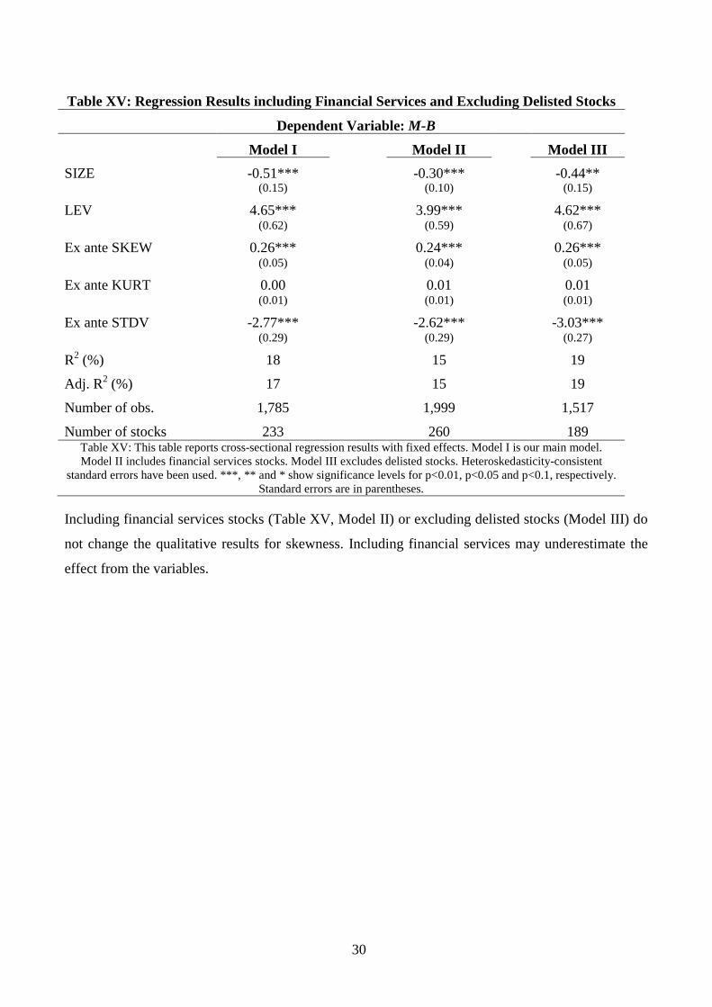
Table XV: Regression Results including Financial Services and Excluding Delisted Stocks

Dependent Variable: M-B Model I Model II Model III SIZE -0.51*** -0.30*** -0.44**

(0.15) (0.10) (0.15)

LEV 4.65*** 3.99*** 4.62*** (0.62) (0.59) (0.67)

Ex ante SKEW 0.26*** 0.24*** 0.26*** (0.05) (0.04) (0.05)

Ex ante KURT 0.00 0.01 0.01 (0.01) (0.01) (0.01)

Ex ante STDV -2.77*** -2.62*** -3.03*** (0.29) (0.29) (0.27)

R2 (%) 18 15 19

Adj. R2 (%) 17 15 19

Number of obs. 1,785 1,999 1,517

Number of stocks 233 260 189 Table XV: This table reports cross-sectional regression results with fixed effects. Model I is our main model. Model II includes financial services stocks. Model III excludes delisted stocks. Heteroskedasticity-consistent

standard errors have been used. ***, ** and * show significance levels for p<0.01, p<0.05 and p<0.1, respectively. Standard errors are in parentheses.

Including financial services stocks (Table XV, Model II) or excluding delisted stocks (Model III) do

not change the qualitative results for skewness. Including financial services may underestimate the

effect from the variables.

31

Winsorization

Graph II: Density Graph for Winsorized Skewness

Graph II: Density graphs for skewness (non-winsorized), skewness winsorized at 5% and 10% fraction, respectively.