investor sentiment and the cross-section of stock...
TRANSCRIPT

THE JOURNAL OF FINANCE • VOL. LXI, NO. 4 • AUGUST 2006
Investor Sentiment and the Cross-Sectionof Stock Returns
MALCOLM BAKER and JEFFREY WURGLER∗
ABSTRACT
We study how investor sentiment affects the cross-section of stock returns. We pre-
dict that a wave of investor sentiment has larger effects on securities whose valua-
tions are highly subjective and difficult to arbitrage. Consistent with this prediction,
we find that when beginning-of-period proxies for sentiment are low, subsequent re-
turns are relatively high for small stocks, young stocks, high volatility stocks, un-
profitable stocks, non-dividend-paying stocks, extreme growth stocks, and distressed
stocks. When sentiment is high, on the other hand, these categories of stock earn
relatively low subsequent returns.
CLASSICAL FINANCE THEORY LEAVES NO ROLE FOR INVESTOR SENTIMENT. Rather, thistheory argues that competition among rational investors, who diversify to opti-mize the statistical properties of their portfolios, will lead to an equilibrium inwhich prices equal the rationally discounted value of expected cash flows, andin which the cross-section of expected returns depends only on the cross-sectionof systematic risks.1 Even if some investors are irrational, classical theory ar-gues, their demands are offset by arbitrageurs and thus have no significantimpact on prices.
In this paper, we present evidence that investor sentiment may have signifi-cant effects on the cross-section of stock prices. We start with simple theoreticalpredictions. Because a mispricing is the result of an uninformed demand shockin the presence of a binding arbitrage constraint, we predict that a broad-based wave of sentiment has cross-sectional effects (that is, does not simplyraise or lower all prices equally) when sentiment-based demands or arbitrage
∗Baker is at the Harvard Business School and National Bureau of Economic Research; Wurgler
is at the NYU Stern School of Business and the National Bureau of Economic Research. We thank
an anonymous referee, Rob Stambaugh (the editor), Ned Elton, Wayne Ferson, Xavier Gabaix,
Marty Gruber, Lisa Kramer, Owen Lamont, Martin Lettau, Anthony Lynch, Jay Shanken, Meir
Statman, Sheridan Titman, and Jeremy Stein for helpful comments, as well as participants of
conferences or seminars at Baruch College, Boston College, the Chicago Quantitative Alliance,
Emory University, the Federal Reserve Bank of New York, Harvard University, Indiana University,
Michigan State University, NBER, the Norwegian School of Economics and Business, Norwegian
School of Management, New York University, Stockholm School of Economics, Tulane University,
the University of Amsterdam, the University of British Columbia, the University of Illinois, the
University of Kentucky, the University of Michigan, the University of Notre Dame, the University
of Texas, and the University of Wisconsin. We gratefully acknowledge financial support from the
Q Group and the Division of Research of the Harvard Business School.1 See Gomes, Kogan, and Zhang (2003) for a recent model in this tradition.
1645

1646 The Journal of Finance
constraints vary across stocks. In practice, these two distinct channels lead toquite similar predictions because stocks that are likely to be most sensitive tospeculative demand, those with highly subjective valuations, also tend to bethe riskiest and costliest to arbitrage. Concretely, then, theory suggests twodistinct channels through which the shares of certain firms—newer, smaller,more volatile, unprofitable, non-dividend paying, distressed or with extremegrowth potential, and firms with analogous characteristics—are likely to bemore affected by shifts in investor sentiment.
To investigate this prediction empirically, and to get a more tangible sense ofthe intrinsically elusive concept of investor sentiment, we start with a summaryof the rises and falls in U.S. market sentiment from 1961 through the Internetbubble. This summary is based on anecdotal accounts and thus by its naturecan only be a suggestive, ex post characterization of fluctuations in sentiment.Nonetheless, its basic message appears broadly consistent with our theoreticalpredictions and suggests that more rigorous tests are warranted.
Our main empirical approach is as follows. Because cross-sectional patternsof sentiment-driven mispricing would be difficult to identify directly, we ex-amine whether cross-sectional predictability patterns in stock returns dependupon proxies for beginning-of-period sentiment. For example, low future returnson young firms relative to old firms, conditional on high values for proxies forbeginning-of-period sentiment, would be consistent with the ex ante relativeovervaluation of young firms. As usual, we are mindful of the joint hypothesisproblem that any predictability patterns we find actually reflect compensationfor systematic risks.
The first step is to gather proxies for investor sentiment that we can use astime-series conditioning variables. Since there are no perfect and/or uncontro-versial proxies for investor sentiment, our approach is necessarily practical.Specifically, we consider a number of proxies suggested in recent work andform a composite sentiment index based on their first principal component. Toreduce the likelihood that these proxies are connected to systematic risk, wealso form an index based on sentiment proxies that have been orthogonalized toseveral macroeconomic conditions. The sentiment indexes visibly line up withhistorical accounts of bubbles and crashes.
We then test how the cross-section of subsequent stock returns varies withbeginning-of-period sentiment. Using monthly stock returns between 1963 and2001, we start by forming equal-weighted decile portfolios based on several firmcharacteristics. (Our theory predicts, and the empirical results confirm, thatlarge firms will be less affected by sentiment, and hence value weighting willtend to obscure the relevant patterns.) We then look for patterns in the averagereturns across deciles conditional upon the beginning-of-period level of senti-ment. We find that when sentiment is low (below sample average), small stocksearn particularly high subsequent returns, but when sentiment is high (aboveaverage), there is no size effect at all. Conditional patterns are even sharperwhen we sort on other firm characteristics. When sentiment is low, subsequentreturns are higher on very young (newly listed) stocks than older stocks, high-return volatility than low-return volatility stocks, unprofitable stocks thanprofitable ones, and nonpayers than dividend payers. When sentiment is high,

Investor Sentiment and the Cross-Section of Stock Returns 1647
these patterns completely reverse. In other words, several characteristics thatdo not have any unconditional predictive power actually display sign-flippingpredictive ability, in the hypothesized directions, once one conditions on senti-ment. These are our most striking findings. Although earlier data are not asrich, some of these patterns are also apparent in a sample that covers 1935through 1961.
The sorts also suggest that sentiment affects extreme growth and distressedfirms in similar ways. Note that when stocks are sorted into deciles by salesgrowth, book-to-market, or external financing activity, growth and distressfirms tend to lie at opposing extremes, with more “stable” firms in the middledeciles. We find that when sentiment is low, the subsequent returns on stocks atboth extremes are especially high relative to their unconditional average, whilestocks in the middle deciles are less affected by sentiment. (The result is notstatistically significant for book-to-market, however.) This U-shaped patternin the conditional difference is also broadly consistent with theoretical pre-dictions: both extreme growth and distressed firms have relatively subjectivevaluations and are relatively hard to arbitrage, and so they should be expectedto be most affected by sentiment. Again, note that this intriguing conditionalpattern would be averaged away in an unconditional study.
We then consider a regression approach, which allows us to control for co-movement in size and book-to-market-sorted stocks using the Fama-French(1993) factors. We use the sentiment indexes to forecast the returns of varioushigh-minus-low portfolios (in terms of sensitivity to sentiment). Not surpris-ingly, given that our decile portfolios are equal-weighted and several of thecharacteristics we examine are correlated with size, the inclusion of SMB asa control tends to reduce the magnitude of the predictability, although somepredictive power generally remains.
We then turn to the classical alternative explanation, namely, that they sim-ply reflect a complex pattern of compensation for systematic risk. This expla-nation would account for the predictability evidence by either time variationin rational, market-wide risk premia or time variation in the cross-sectionalpattern of risk, that is, beta loadings. Further tests cast doubt on these hy-potheses. We test the second possibility directly and find no link between thepatterns in predictability and patterns in betas with market returns or con-sumption growth. If risk is not changing over time, then the first possibilityrequires not just time variation in risk premia, but also changes in sign. Putsimply, it would require that in half of our sample period (when sentiment isrelatively low), older, less volatile, profitable, and/or dividend-paying firms ac-tually require a risk premium over very young, highly volatile, unprofitable,and/or nonpayers. This is counterintuitive. Other aspects of the results alsosuggest that systematic risk is not a complete explanation.
The results challenge the classical view of the cross-section of stock pricesand, in doing so, build on several recent themes. First, the results complementearlier work that shows sentiment helps to explain the time series of returns(Kothari and Shanken (1997), Neal and Wheatley (1998), Shiller (1981, 2000),Baker and Wurgler (2000)). Campbell and Cochrane (2000), Wachter (2000),Lettau and Ludvigson (2001), and Menzly, Santos, and Veronesi (2004) examine

1648 The Journal of Finance
the effects of conditional systematic risks; here we condition on investor sen-timent. Daniel and Titman (1997) test a characteristics-based model for thecross-section of expected returns; we extend their specification into a condi-tional characteristics-based model. Shleifer (2000) surveys early work on sen-timent and limited arbitrage, two key ingredients here. Barberis and Shleifer(2003), Barberis, Shleifer, and Wurgler (2005), and Peng and Xiong (2004) dis-cuss category-level trading, and Fama and French (1993) document comove-ment of stocks of similar sizes and book-to-market ratios; uninformed demandshocks for categories of stocks with similar characteristics are central to ourresults. Finally, we extend and unify known relationships among sentiment,IPOs, and small stock returns (Lee, Shleifer, and Thaler (1991), Swaminathan(1996), Neal and Wheatley (1998)).
Section I discusses theoretical predictions. Section II provides a qualitativehistory of recent speculative episodes. Section III describes our empirical hy-potheses and data, and Section IV presents the main empirical tests. Section Vconcludes.
I. Theoretical Effects of Sentiment on the Cross-Section
A mispricing is the result of both an uninformed demand shock and a limiton arbitrage. One can therefore think of two distinct channels through whichinvestor sentiment, as defined more precisely below, might affect the cross-section of stock prices. In the first channel, sentimental demand shocks varyin the cross-section, while arbitrage limits are constant. In the second, thedifficulty of arbitrage varies across stocks but sentiment is generic. We discussthese in turn.
A. Cross-Sectional Variation in Sentiment
One possible definition of investor sentiment is the propensity to speculate.2
Under this definition, sentiment drives the relative demand for speculativeinvestments, and therefore causes cross-sectional effects even if arbitrage forcesare the same across stocks.
What makes some stocks more vulnerable to broad shifts in the propensityto speculate? We suggest that the main factor is the subjectivity of their valu-ations. For instance, consider a canonical young, unprofitable, extreme growthstock. The lack of an earnings history combined with the presence of appar-ently unlimited growth opportunities allows unsophisticated investors to de-fend, with equal plausibility, a wide spectrum of valuations, from much too lowto much too high, as suits their sentiment. During a bubble period, when thepropensity to speculate is high, this profile of characteristics also allows invest-ment bankers (or swindlers) to further argue for the high end of valuations. Bycontrast, the value of a firm with a long earnings history, tangible assets, and
2 Aghion and Stein (2004) develop a model with both rational expectations and bounded ratio-
nality in which investors periodically emphasize growth over profitability. While the emphasis is
on the corporate and macroeconomic effects, the bounded-rationality version of the model offers
some similar predictions for the cross-section of returns.

Investor Sentiment and the Cross-Section of Stock Returns 1649
stable dividends is much less subjective, and thus its stock is likely to be lessaffected by fluctuations in the propensity to speculate.3
While the above channel suggests how variation in the propensity to spec-ulate may generally affect the cross-section, it does not take a stand on howsentimental investors actually choose stocks. We suggest that they simply de-mand stocks that have the bundle of salient characteristics that is compatiblewith their sentiment.4 That is, investors with a low propensity to speculate maydemand profitable, dividend-paying stocks not because profitability and divi-dends are correlated with some unobservable firm property that defines safetyto the investor, but precisely because the salient characteristics “profitability”and “dividends” are essentially taken to define safety.5 Likewise, the salientcharacteristics “no earnings,” “young age,” and “no dividends” mark the stockas speculative. Casual observation suggests that such an investment processmay be a more accurate description of how typical investors pick stocks thanthe process outlined by Markowitz (1959), in which investors view individualsecurities purely in terms of their statistical properties.
B. Cross-Sectional Variation in Arbitrage
One might also define investor sentiment as optimism or pessimism aboutstocks in general. Indiscriminate waves of sentiment still affect the cross-section, however, if arbitrage forces are relatively weaker in a subset of stocks.
This channel is better understood than the cross-sectional variation in senti-ment channel. A body of theoretical and empirical research shows that arbitragetends to be particularly risky and costly for young, small, unprofitable, extremegrowth, or distressed stocks. First, their high idiosyncratic risk makes relative-value arbitrage especially risky (Wurgler and Zhuravskaya (2002)). Moreover,such stocks tend to be more costly to trade (Amihud and Mendelsohn (1986))and particularly expensive, sometimes impossible, to sell short (D’Avolio (2002),Geczy, Musto, and Reed (2002), Jones and Lamont (2002), Duffie, Garleanu, and
3 The favorite-longshot bias in racetrack betting is a static illustration of the notion that investors
with a high propensity to speculate (racetrack bettors) have a relatively high demand for the most
speculative bets (longshots have the most negative expected returns; see Hausch and Ziemba
(1995)).4 The idea that investors view securities as a vector of salient characteristics borrows from
Lancaster (1966, 1971), who views consumer demand theory from the perspective that the utility
of a consumer good (e.g, oranges) derives from more primitive characteristics (fiber and vitamin C).5 The implications of categorization for finance are explored by Baker and Wurgler (2003),
Barberis and Shleifer (2003), Barberis, Shleifer, and Wurgler (2005), Greenwood and Sosner (2003),
and Peng and Xiong (2004). Note that if investors infer category membership from salient char-
acteristics (some psychologists propose that category membership is determined by the presence
of defining or characteristic features, see, for example, Smith, Shoben, and Rips (1974)), then
sentiment-driven demand will be directly connected to characteristics even if sentimental investors
undertake an intervening process of categorization and trade entirely at the category level. It is
also empirically convenient to boil key investment categories down into vectors of stable and mea-
surable characteristics: One can use the same empirical framework to study episodes such as the
late 1960s growth stocks bubble and the Internet bubble. In other words, the term “Internet bub-
ble” is interesting, but it does not make for a useful or testable theory. The key is to examine the
recurring underlying characteristics.

1650 The Journal of Finance
Pedersen (2002), Lamont and Thaler (2003), Mitchell, Pulvino, and Stafford(2002)). Further, their lower liquidity also exposes would-be arbitrageurs topredatory attacks (Brunnermeier and Pedersen (2005)).
The key point of this discussion is that, in practice, the same stocks that arethe hardest to arbitrage also tend to be the most difficult to value. While forexpositional purposes we have outlined the two channels separately, they arelikely to have overlapping effects. This may make them difficult to distinguishempirically; however, it only strengthens our predictions about what region ofthe cross-section is most affected by sentiment. Indeed, the two channels can re-inforce each other. For example, the fact that investors can convince themselvesof a wide range of valuations in some regions of the cross-section generates anoise-trader risk that further deters short-horizon arbitrageurs (De Long et al.(1990), Shleifer and Vishny (1997)).6
II. An Anecdotal History of Investor Sentiment, 1961–2002
Here we briefly summarize the most prominent U.S. stock market bubblesbetween 1961 and 2002 (matching the period of our main data). The reader ea-ger to see results may skip this section, but it is useful for three reasons. First,despite great interest in the effects of investor sentiment, the academic litera-ture does not contain even the most basic ex post characterization of most of therecent speculative episodes. Second, a knowledge of the rough timing of theseepisodes allows us to make a preliminary judgment about the accuracy of thequantitative proxies for sentiment that we develop later. Third, the discussionsheds some initial, albeit anecdotal, light on the plausibility of our theoreticalpredictions.
We distill our brief history of sentiment from several sources. Kindleberger(2001) draws general lessons from bubbles and crashes over the past few hun-dred years, while Brown (1991), Dreman (1979), Graham (1973), Malkiel (1990,1999), Shiller (2000), and Siegel (1998) focus more specifically on recent U.S.stock market episodes. We take each of these accounts with a grain of salt, andemphasize only those themes that appear repeatedly.
We start in 1961, a year that Graham (1973), Malkiel (1990) and Brown(1991) note as characterized by a high demand for small, young, growth stocks;Dreman (1979, p. 70) confirms their accounts. For instance, Malkiel writes ofa “new-issue mania” that was concentrated on new “tronics” firms. “ . . . Thetronics boom came back to earth in 1962. The tailspin started early in the yearand exploded in a horrendous selling wave . . . Growth stocks took the brunt ofthe decline, falling much further than the general market” (p. 54–57).
The next major bubble developed in 1967 and 1968. Brown writes that“scores of franchisers, computer firms, and mobile home manufactures seemed
6 We do not incorporate the equilibrium prediction of DeLong et al. (1990), namely that securities
with more exposure to sentiment have higher unconditional expected returns. Elton, Gruber, and
Busse (1998) argue that expected returns are not higher on stocks that have higher sensitivities
to the closed-end fund discount. However, Brown et al. (2003) argue that exposure to a sentiment
factor constructed from daily mutual fund flows is a priced factor in the United States and Japan.
Investor Sentiment and the Cross-Section of Stock Returns 1651
to promise overnight wealth . . . . [while] quality was pretty much forgotten”(p. 90). Malkiel and Dreman also note this pattern of a focus on firms withstrong earnings growth or potential and an avoidance of “the major industrialgiants, ‘buggywhip companies,’ as they were sometimes contemptuously called”(Dreman 1979, p. 74–75). Another characteristic apparently out of favor wasdividends. According to the New York Times, “during the speculative marketof the late 1960s many brokers told customers that it didn’t matter whether acompany paid a dividend—just so long as its stock kept going up” (9/13/1976).But “after 1968, as it became clear that capital losses were possible, investorscame to value dividends” (10/7/1999). In summarizing the performance of stocksfrom the end of 1968 through August 1971, Graham (1973) writes: “[our] com-parative results undoubtedly reflect the tendency of smaller issues of inferiorquality to be relatively overvalued in bull markets, and not only to suffer moreserious declines than the stronger issues in the ensuing price collapse, but alsoto delay their full recovery—in many cases indefinitely” (p. 212).
Anecdotal accounts invariably describe the early 1970s as a bear market,with sentiment at a low level. However, a set of established, large, stable, con-sistently profitable stocks known as the “nifty fifty” enjoyed notably high val-uations. Brown (1991), Malkiel (1990), and Siegel (1998) each highlight thisepisode. Siegel writes, “All of these stocks had proven growth records, contin-ual increases in dividends . . . and high market capitalization” (p. 106). Note thatthis speculative episode is a mirror image of those described above (and below).That is, the bubbles associated with high sentiment periods centered on small,young, unprofitable growth stocks, whereas the nifty fifty episode appears tobe a bubble in a set of firms with an opposite set of characteristics (old, large,and continuous earnings and dividend growth) that happened in a period of lowsentiment.
The late 1970s through mid 1980s are described as a period of generallyhigh sentiment, perhaps associated with Reagan-era optimism. This periodwitnessed a series of speculative episodes. Dreman describes a bubble in gam-bling issues in 1977 and 1978. Ritter (1984) studies the hot-issue market of1980, and finds greater initial returns on IPOs of natural resource start-upsthan on large, mature, profitable offerings. Of 1983, Malkiel (p. 74–75) writesthat “the high-technology new-issue boom of the first half of 1983 was an al-most perfect replica of the 1960’s episodes . . . The bubble appears to have burstearly in the second half of 1983 . . . the carnage in the small company and new-issue markets was truly catastrophic.” Brown confirms this account. Of themid 1980s, Malkiel writes that “What electronics was to the 1960s, biotech-nology became to the 1980s . . . . new issues of biotech companies were eagerlygobbled up . . . . having positive sales and earnings was actually considered adrawback” (p. 77–79). But by 1987 and 1988, “market sentiment had changedfrom an acceptance of an exciting story . . . to a desire to stay closer to earth withlow-multiple stocks that actually pay dividends” (p. 79).
The late 1990s bubble in technology stocks is familiar. By all accounts, in-vestor sentiment was broadly high before the bubble started to burst in 2000.Cochrane (2003) and Ofek and Richardson (2002) offer ex post perspectives on
1652 The Journal of Finance
the bubble, while Asness et al. (2000) and Chan, Karceski, and Lakonishok(2000) were arguing even before the crash that late 1990s growth stockvaluations were difficult to ascribe to rationally expected earnings growth.Malkiel draws parallels to episodes in the 1960s, 1970s, and 1980s, and Shiller(2000) draws parallels to the late 1920s. As in earlier speculative episodes thatoccurred in high sentiment periods, demand for dividend payers seems to havebeen low (New York Times, 1/6/1998). Ljungqvist and Wilhelm (2003) find that80% of the 1999 and 2000 IPO cohorts had negative earnings per share andthat the median age of 1999 IPOs was 4 years. This contrasts with an averageage of over 9 years just prior to the emergence of the bubble, and of over 12years by 2001 and 2002 (Ritter (2003)).
These anecdotes suggest some regular patterns in the effect of investor senti-ment on the cross-section. For instance, canonical extreme growth stocks seemto be especially prone to bubbles (and subsequent crashes), consistent with theobservation that they are more appealing to speculators and optimists and atthe same time hard to arbitrage. The “nifty fifty” bubble is a notable excep-tion, but anecdotal accounts suggest that this bubble occurred during a periodof broadly low sentiment, so it may still be consistent with the cross-sectionalprediction that an increase in sentiment increases the relative price of thosestocks that are the most subjective to value and the hardest to arbitrage. Wenow turn to formal tests of this prediction.
III. Empirical Approach and Data
A. Empirical Approach
Theory and historical anecdote both suggest that sentiment may cause sys-tematic patterns of mispricing. Because mispricing is hard to identify directly,however, our approach is to look for systematic patterns of mispricing correc-tion. For example, a pattern in which returns on young and unprofitable growthfirms are (on average) especially low when beginning-of-period sentiment is es-timated to be high may represent the correction of a bubble in growth stocks.
Specifically, to identify sentiment-driven changes in cross-sectional pre-dictability patterns, we need to control for two more basic effects, namely, thegeneric impact of investor sentiment on all stocks and the generic impact ofcharacteristics across all time periods. Thus, we organize our analysis looselyaround the following predictive specification:
Et−1[Rit] = a + a1Tt−1 + b′1xit−1 + b′
2Tt−1xit−1, (1)
where i indexes firms, t denotes time, x is a vector of characteristics, and T is aproxy for sentiment. The coefficient a1 picks up the generic effect of sentiment,and the vector b1 the generic effect of characteristics. Our interest centers onb2. The null is that b2 equals zero or, more precisely, that any nonzero effect isrational compensation for systematic risk. The alternative is that b2 is nonzeroand reveals cross-sectional patterns in sentiment-driven mispricing. We callEquation (1) a “conditional characteristics model” because it adds conditionalterms to the characteristics model of Daniel and Titman (1997).

Investor Sentiment and the Cross-Section of Stock Returns 1653
B. Characteristics and Returns
The firm-level data are from the merged CRSP-Compustat database. Thesample includes all common stock (share codes 10 and 11) between 1962 through2001. Following Fama and French (1992), we match accounting data for fiscalyear-ends in calendar year t − 1 to (monthly) returns from July t through Junet + 1, and we use their variable definitions when possible.
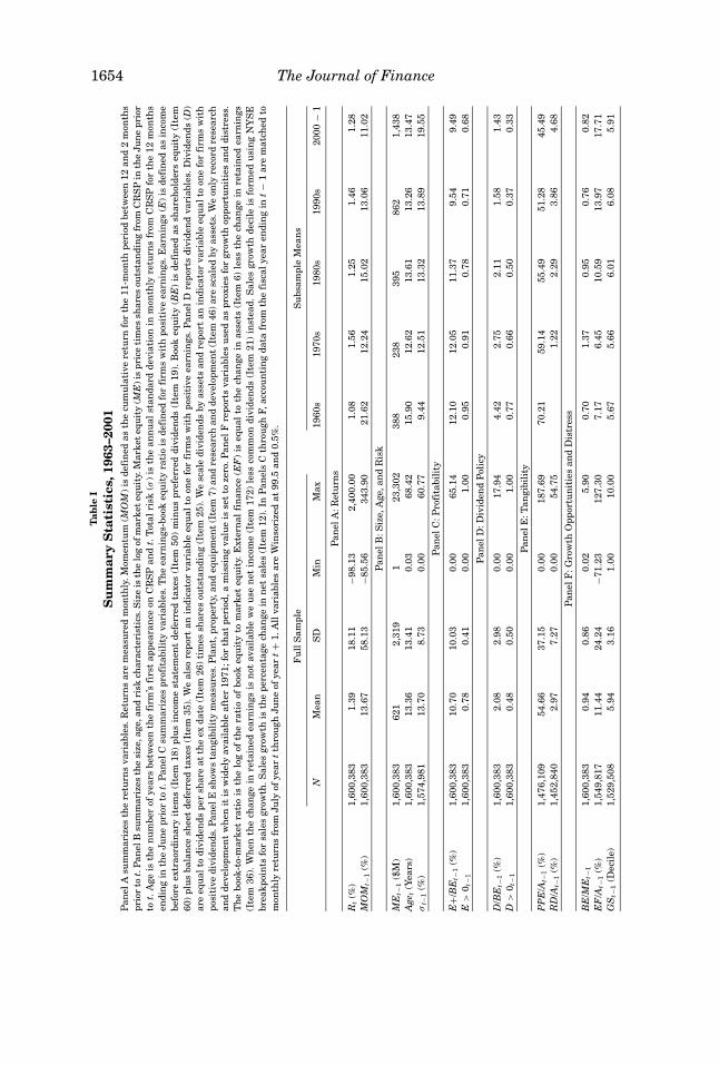
Table I shows summary statistics. Panel A summarizes returns variables.Following common practice, we define momentum, MOM, as the cumulativeraw return for the 11-month period from 12 through 2 months prior to theobservation return. Because momentum is not mentioned as a salient charac-teristic in historical anecdote, and theory does not suggest a direct connectionbetween momentum and the difficulty of valuation or arbitrage, we use mo-mentum merely as a control variable to understand the independence of ourresults from known mispricing patterns.
The remaining panels summarize the firm and security characteristics thatwe consider. The previous sections’ discussions point us directly to several vari-ables. To that list, we add a few more characteristics that, by introspection,seem likely to be salient to investors. Overall, we roughly group characteristicsas pertaining to firm size and age, profitability, dividends, asset tangibility, andgrowth opportunities and/or distress.
Size and age characteristics include market equity, ME, from June of yeart, measured as price times shares outstanding from CRSP. We match ME tomonthly returns from July of year t through June of year t + 1. Firm age, Age,is the number of years since the firm’s first appearance on CRSP, measured tothe nearest month,7 and Sigma is the standard deviation of monthly returnsover the 12 months ending in June of year t. If there are at least nine returnsavailable to estimate it, Sigma is then matched to monthly returns from Julyof year t through June of year t + 1. While historical anecdote does not identifystock volatility itself as a salient characteristic, prior work argues that it islikely to be a good proxy for the difficulty of both valuation and arbitrage.
Profitability characteristics include the return on equity, E+/BE, which ispositive for profitable firms and zero for unprofitable firms. Earnings (E) isincome before extraordinary items (Item 18) plus income statement deferredtaxes (Item 50) minus preferred dividends (Item 19), if earnings are positive;book equity (BE) is shareholders equity (Item 60) plus balance sheet deferredtaxes (Item 35). The profitability dummy variable E > 0 takes the value onefor profitable firms and zero for unprofitable firms.
Dividend characteristics include dividends to equity, D/BE, which is divi-dends per share at the ex date (Item 26) times Compustat shares outstanding(Item 25) divided by book equity. The dividend payer dummy D > 0 takes thevalue one for firms with positive dividends per share by the ex date. The declinenoted by Fama and French (2001) in the percentage of firms that pay dividendsis apparent.
7 Barry and Brown (1984) use the more accurate term “period of listing.” A large number of firms
appear on CRSP for the first time in December 1972, when Nasdaq coverage begins. Excluding these
firms from our analyses of age does not change any of our inferences.
1654 The Journal of FinanceT
able
I
Su
mm
ary
Sta
tist
ics,
1963
–200
1P
an
el
Asu
mm
ari
zes
the
retu
rns
va
ria
ble
s.R
etu
rns
are
mea
sure
dm
on
thly
.M
om
en
tum
(MO
M)
isd
efi
ned
as
the
cum
ula
tive
retu
rnfo
rth
e1
1-m
on
thp
eri
od
betw
een
12
an
d2
mon
ths
pri
or
tot.
Pa
nel
Bsu
mm
ari
zes
the
size
,a
ge,a
nd
risk
cha
ract
eri
stic
s.S
ize
isth
elo
gof
ma
rket
eq
uit
y.M
ark
et
eq
uit
y(M
E)
isp
rice
tim
es
sha
res
ou
tsta
nd
ing
from
CR
SP
inth
eJu
ne
pri
or
tot.
Age
isth
en
um
ber
of
yea
rsb
etw
een
the
firm
’sfi
rst
ap
pea
ran
ceon
CR
SP
an
dt.
Tota
lri
sk(σ
)is
the
an
nu
al
sta
nd
ard
devia
tion
inm
on
thly
retu
rns
from
CR
SP
for
the
12
mon
ths
en
din
gin
the
Ju
ne
pri
or
tot.
Pa
nel
Csu
mm
ari
zes
pro
fita
bil
ity
va
ria
ble
s.T
he
ea
rnin
gs-
book
eq
uit
yra
tio
isd
efi
ned
for
firm
sw
ith
posi
tive
ea
rnin
gs.
Ea
rnin
gs
(E)
isd
efi
ned
as
inco
me
befo
reextr
aord
ina
ryit
em
s(I
tem
18
)p
lus
inco
me
sta
tem
en
td
efe
rred
taxes
(Ite
m5
0)
min
us
pre
ferr
ed
div
iden
ds
(Ite
m1
9).
Book
eq
uit
y(B
E)
isd
efi
ned
as
sha
reh
old
ers
eq
uit
y(I
tem
60
)p
lus
ba
lan
cesh
eet
defe
rred
taxes
(Ite
m3
5).
We
als
ore
port
an
ind
ica
tor
va
ria
ble
eq
ua
lto
on
efo
rfi
rms
wit
hp
osi
tive
ea
rnin
gs.
Pa
nel
Dre
port
sd
ivid
en
dva
ria
ble
s.D
ivid
en
ds
(D)
are
eq
ua
lto
div
iden
ds
per
sha
rea
tth
eex
da
te(I
tem
26
)ti
mes
sha
res
ou
tsta
nd
ing
(Ite
m2
5).
We
sca
led
ivid
en
ds
by
ass
ets
an
dre
port
an
ind
ica
tor
va
ria
ble
eq
ua
lto
on
efo
rfi
rms
wit
h
posi
tive
div
iden
ds.
Pa
nel
Esh
ow
sta
ngib
ilit
ym
ea
sure
s.P
lan
t,p
rop
ert
y,a
nd
eq
uip
men
t(I
tem
7)
an
dre
sea
rch
an
dd
evelo
pm
en
t(I
tem
46
)a
resc
ale
db
ya
ssets
.W
eon
lyre
cord
rese
arc
h
an
dd
evelo
pm
en
tw
hen
itis
wid
ely
ava
ila
ble
aft
er
19
71
;fo
rth
at
peri
od
,a
mis
sin
gva
lue
isse
tto
zero
.P
an
el
Fre
port
sva
ria
ble
su
sed
as
pro
xie
sfo
rgro
wth
op
port
un
itie
sa
nd
dis
tress
.
Th
eb
ook
-to-m
ark
et
rati
ois
the
log
of
the
rati
oof
book
eq
uit
yto
ma
rket
eq
uit
y.E
xte
rna
lfi
na
nce
(EF
)is
eq
ua
lto
the
cha
nge
ina
ssets
(Ite
m6
)le
ssth
ech
an
ge
inre
tain
ed
ea
rnin
gs
(Ite
m3
6).
Wh
en
the
cha
nge
inre
tain
ed
ea
rnin
gs
isn
ot
ava
ila
ble
we
use
net
inco
me
(Ite
m1
72
)le
ssco
mm
on
div
iden
ds
(Ite
m2
1)
inst
ea
d.
Sa
les
gro
wth
deci
leis
form
ed
usi
ng
NY
SE
bre
ak
poin
tsfo
rsa
les
gro
wth
.S
ale
sgro
wth
isth
ep
erc
en
tage
cha
nge
inn
et
sale
s(I
tem
12
).In
Pa
nels
Cth
rou
gh
F,
acc
ou
nti
ng
da
tafr
om
the
fisc
al
yea
ren
din
gin
t−
1a
rem
atc
hed
to
mon
thly
retu
rns
from
Ju
lyof
yea
rt
thro
ugh
Ju
ne
of
yea
rt+
1.
All
va
ria
ble
sa
reW
inso
rize
da
t9
9.5
an
d0
.5%
.
Fu
llS
am
ple
Su
bsa
mp
leM
ea
ns
NM
ea
nS
DM
inM
ax
19
60
s1
97
0s
19
80
s1
99
0s
20
00
−1
Pa
nel
A:
Retu
rns
Rt
(%)
1,6
00
,38
31
.39
18
.11
−98
.13
2,4
00
.00
1.0
81
.56
1.2
51
.46
1.2
8
MO
Mt−
1(%
)1
,60
0,3
83
13
.67
58
.13
−85
.56
34
3.9
02
1.6
21
2.2
41
5.0
21
3.0
61
1.0
2
Pa
nel
B:
Siz
e,
Age,
an
dR
isk
ME
t−1
($M
)1
,60
0,3
83
62
12
,31
91
23
,30
23
88
23
83
95
86
21
,43
8
Age
t(Y
ea
rs)
1,6
00
,38
31
3.3
61
3.4
10
.03
68
.42
15
.90
12
.62
13
.61
13
.26
13
.47
σt−
1(%
)1
,57
4,9
81
13
.70
8.7
30
.00
60
.77
9.4
41
2.5
11
3.3
21
3.8
91
9.5
5
Pa
nel
C:
Pro
fita
bil
ity
E+/
BE
t−1
(%)
1,6
00
,38
31
0.7
01
0.0
30
.00
65
.14
12
.10
12
.05
11
.37
9.5
49
.49
E>
0t−
11
,60
0,3
83
0.7
80
.41
0.0
01
.00
0.9
50
.91
0.7
80
.71
0.6
8
Pa
nel
D:
Div
iden
dP
oli
cy
D/B
Et−
1(%
)1
,60
0,3
83
2.0
82
.98
0.0
01
7.9
44
.42
2.7
52
.11
1.5
81
.43
D>
0t−
11
,60
0,3
83
0.4
80
.50
0.0
01
.00
0.7
70
.66
0.5
00
.37
0.3
3
Pa
nel
E:
Ta
ngib
ilit
y
PP
E/A
t−1
(%)
1,4
76
,10
95
4.6
63
7.1
50
.00
18
7.6
97
0.2
15
9.1
45
5.4
95
1.2
84
5.4
9
RD
/At−
1(%
)1
,45
2,8
40
2.9
77
.27
0.0
05
4.7
51
.22
2.2
93
.86
4.6
8
Pa
nel
F:
Gro
wth
Op
port
un
itie
sa
nd
Dis
tress
BE
/ME
t−1
1,6
00
,38
30
.94
0.8
60
.02
5.9
00
.70
1.3
70
.95
0.7
60
.82
EF
/At−
1(%
)1
,54
9,8
17
11
.44
24
.24
−71
.23
12
7.3
07
.17
6.4
51
0.5
91
3.9
71
7.7
1
GS
t−1
(Deci
le)
1,5
29
,50
85
.94
3.1
61
.00
10
.00
5.6
75
.66
6.0
16
.08
5.9
1
Investor Sentiment and the Cross-Section of Stock Returns 1655
The referee suggests that asset tangibility may proxy for the difficulty ofvaluation. Asset tangibility characteristics are measured by property, plantand equipment (Item 7) over assets, PPE/A, and research and developmentexpense over assets (Item 46), RD/A. One concern is the coverage of the R&Dvariable. We do not consider this variable prior to 1972, because the FinancialAccounting Standards Board did not require R&D to be expensed until 1974and Compustat coverage prior to 1972 is very poor. Also, even in recent yearsless than half of the sample reports positive R&D.
Characteristics indicating growth opportunities, distress, or both includebook-to-market equity, BE/ME, whose elements are defined above. Externalfinance, EF/A, is the change in assets (Item 6) minus the change in retainedearnings (Item 36) divided by assets. Sales growth (GS) is the change in net sales(Item 12) divided by prior-year net sales. Sales growth GS/10 is the decile of thefirm’s sales growth in the prior year relative to NYSE firms’ decile breakpoints.
As will become clear below, one must grasp the multidimensional nature ofthe growth and distress variables in order to understand how they interact withsentiment. In particular, book-to-market wears at least three hats: High valuesmay indicate distress; low values may indicate high growth opportunities; and,as a scaled-price variable, book-to-market is also a generic valuation indicatorthat varies with any source of mispricing or rational expected returns. Sim-ilarly, sales growth and external finance wear at least two hats: Low values(which are negative) may indicate distress, and high values may reflect growthopportunities. Further, to the extent that market timing motives drive externalfinance, EF/A also wears a third hat as a generic misvaluation indicator.
All explanatory variables are Winsorized each year at their 0.5 and 99.5 per-centiles. Finally, in Panels C through F, the accounting data for fiscal yearsending in calendar year t − 1 are matched to monthly returns from July of yeart through June of year t + 1.
C. Investor Sentiment
Prior work suggests a number of proxies for sentiment to use as time-seriesconditioning variables. There are no definitive or uncontroversial measures,however. We therefore form a composite index of sentiment that is based on thecommon variation in six underlying proxies for sentiment: the closed-end funddiscount, NYSE share turnover, the number and average first-day returns onIPOs, the equity share in new issues, and the dividend premium. The sentimentproxies are measured annually from 1962 to 2001. We first introduce eachproxy separately, and then discuss how they are formed into overall sentimentindexes.
The closed-end fund discount, CEFD, is the average difference between thenet asset values (NAV) of closed-end stock fund shares and their market prices.Prior work suggests that CEFD is inversely related to sentiment. Zweig (1973)uses it to forecast reversion in Dow Jones stocks, and Lee et al. (1991) arguethat sentiment is behind various features of closed-end fund discounts. Wetake the value-weighted average discount on closed-end stock funds for 1962
1656 The Journal of Finance
through 1993 from Neal and Wheatley (1998), for 1994 through 1998 fromCDA/Wiesenberger, and for 1999 through 2001 from turn-of-the-year issues ofthe Wall Street Journal.
NYSE share turnover is based on the ratio of reported share volume to av-erage shares listed from the NYSE Fact Book. Baker and Stein (2004) suggestthat turnover, or more generally liquidity, can serve as a sentiment index: In amarket with short-sales constraints, irrational investors participate, and thusadd liquidity, only when they are optimistic; hence, high liquidity is a symp-tom of overvaluation. Supporting this, Jones (2001) finds that high turnoverforecasts low market returns. Turnover displays an exponential, positive trendover our period and the May 1975 elimination of fixed commissions also has avisible effect. As a partial solution, we define TURN as the natural log of theraw turnover ratio, detrended by the 5-year moving average.
The IPO market is often viewed as sensitive to sentiment, with high first-day returns on IPOs cited as a measure of investor enthusiasm, and the lowidiosyncratic returns on IPOs often interpreted as a symptom of market timing(Stigler (1964), Ritter (1991)). We take the number of IPOs, NIPO, and theaverage first-day returns, RIPO, from Jay Ritter’s website, which updates thesample in Ibbotson, Sindelar, and Ritter (1994).
The share of equity issues in total equity and debt issues is another measure offinancing activity that may capture sentiment. Baker and Wurgler (2000) findthat high values of the equity share predict low market returns. The equityshare is defined as gross equity issuance divided by gross equity plus grosslong-term debt issuance using data from the Federal Reserve Bulletin.8
Our sixth and last sentiment proxy is the dividend premium, PD−ND, the logdifference of the average market-to-book ratios of payers and nonpayers. Bakerand Wurgler (2004) use this variable to proxy for relative investor demand fordividend-paying stocks. Given that payers are generally larger, more profitablefirms with weaker growth opportunities (Fama and French (2001)), the divi-dend premium may proxy for the relative demand for this correlated bundle ofcharacteristics.
Each sentiment proxy is likely to include a sentiment component as well asidiosyncratic, non-sentiment-related components. We use principal componentsanalysis to isolate the common component. Another issue in forming an indexis determining the relative timing of the variables—that is, if they exhibit lead-lag relationships, some variables may reflect a given shift in sentiment earlierthan others. For instance, Ibbotson and Jaffe (1975), Lowry and Schwert (2002),and Benveniste et al. (2003) find that IPO volume lags the first-day returns onIPOs. Perhaps sentiment is partly behind the high first-day returns, and thisattracts additional IPO volume with a lag. More generally, proxies that involvefirm supply responses (S and NIPO) can be expected to lag behind proxies
8 While they both reflect equity issues, the number of IPOs and the equity share have important
differences. The equity share includes seasoned offerings, predicts market returns, and scales by
total external finance to isolate the composition of finance from the level. On the other hand, the
IPO variables may better reflect demand for certain IPO-like regions of the cross-section that
theory and historical anecdote suggest are most sensitive to sentiment.

Investor Sentiment and the Cross-Section of Stock Returns 1657
that are based directly on investor demand or investor behavior (RIPO, PD−ND,TURN, and CEFD).
We form a composite index that captures the common component in the sixproxies and incorporates the fact that some variables take longer to reveal thesame sentiment.9 We start by estimating the first principal component of thesix proxies and their lags. This gives us a first-stage index with 12 loadings,one for each of the current and lagged proxies. We then compute the correla-tion between the first-stage index and the current and lagged values of eachof the proxies. Finally, we define SENTIMENT as the first principal compo-nent of the correlation matrix of six variables—each respective proxy’s lead orlag, whichever has higher correlation with the first-stage index—rescaling thecoefficients so that the index has unit variance.
This procedure leads to a parsimonious index
SENTIMENTt = −0.241CEFDt + 0.242TURNt−1 + 0.253NIPOt
+ 0.257RIPOt−1 + 0.112St − 0.283P D−NDt−1 , (2)
where each of the index components has first been standardized. The firstprincipal component explains 49% of the sample variance, so we conclude thatone factor captures much of the common variation. The correlation between the12-term first-stage index and the SENTIMENT index is 0.95, suggesting thatlittle information is lost in dropping the six terms with other time subscripts.
The SENTIMENT index has several appealing properties. First, each indi-vidual proxy enters with the expected sign. Second, all but one enters withthe expected timing; with the exception of CEFD, price and investor behaviorvariables lead firm supply variables. Third, the index irons out some extremeobservations. (The dividend premium and the first-day IPO returns reachedunprecedented levels in 1999, so for these proxies to work as individual predic-tors in the full sample, these levels must be matched exactly to extreme futurereturns.)
One might object to equation (2) as a measure of sentiment on the groundsthat the principal components analysis cannot distinguish between a commonsentiment component and a common business cycle component. For instance,the number of IPOs varies with the business cycle in part for entirely rationalreasons. We want to identify when the number of IPOs is high for no good reason.We therefore construct a second index that explicitly removes business cyclevariation from each of the proxies prior to the principal components analysis.
Specifically, we regress each of the six raw proxies on growth in the indus-trial production index (Federal Reserve Statistical Release G.17), growth inconsumer durables, nondurables, and services (all from BEA National IncomeAccounts Table 2.10), and a dummy variable for NBER recessions. The residu-als from these regressions, labeled with a superscript ⊥, may be cleaner proxiesfor investor sentiment. We form an index of the orthogonalized proxies followingthe same procedure as before. The resulting index is
9 See Brown and Cliff (2004) for a similar approach to extracting a sentiment factor from a set
of noisy proxies.
1658 The Journal of Finance
SENTIMENT ⊥t = −0.198CEFD⊥
t + 0.225TURN ⊥t−1 + 0.234 NIPO⊥
t
+ 0.263RIPO⊥t−1 + 0.211S ⊥
t − 0.243P D−ND,⊥t−1 . (3)
Here, the first principal component explains 53% of the sample variance of theorthogonalized variables. Moreover, only the first eigenvalue is above 1.00. Interms of the signs and the timing of the components, SENTIMENT⊥ retainsall of the appealing properties of SENTIMENT.
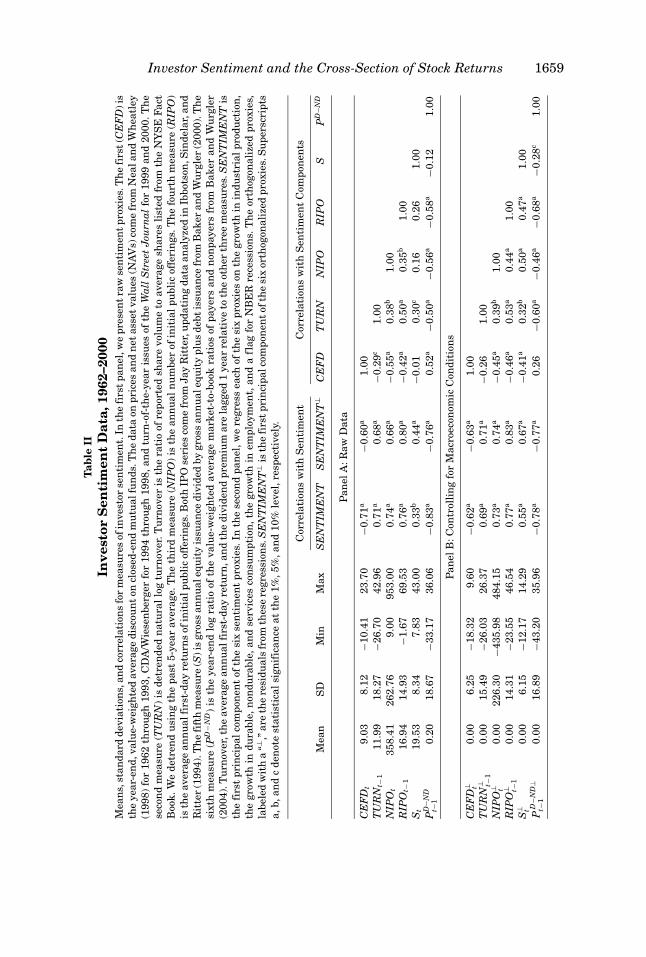
Table II summarizes and correlates the sentiment measures, and Figure 1plots them. The figure shows immediately that orthogonalizing to macro vari-ables is a second-order issue. It does not qualitatively affect any componentof the index or the overall index (see Panel E). Indeed, Table II suggests thaton balance the orthogonalized proxies are slightly more correlated with eachother than are the raw proxies. If the raw variables were driven by commonmacroeconomic conditions (that we failed to remove through orthogonalization)instead of common investor sentiment, one would expect the opposite. In anycase, to demonstrate robustness we present results for both indexes in our mainanalysis.
More importantly, Figure 1 shows that the sentiment measures roughly lineup with anecdotal accounts of fluctuations in sentiment. Most proxies pointto low sentiment in the first few years of the sample, after the 1961 crash ingrowth stocks. Specifically, the closed-end fund discount and dividend premiumare high, while turnover and equity issuance-related variables are low. Eachvariable identifies a spike in sentiment in 1968 and 1969, again matching anec-dotal accounts. Sentiment then tails off until, by the mid 1970s, it is low by mostmeasures (recall that for turnover this is confounded by deregulation). The late1970s through mid 1980s sees generally rising sentiment, and, according tothe composite index, sentiment has not dropped far below a medium level since1980. At the end of 1999, near the peak of the Internet bubble, sentiment is highby most proxies. Overall, SENTIMENT⊥ is positive for the years 1968–1970,1972, 1979–1987, 1994, 1996–1997, and 1999–2001. This correspondence withanecdotal accounts seems to confirm that the measures capture the intendedvariation.
There are other variables that one might reasonably wish to include in asentiment index. The main constraint is availability and consistent measure-ment over the 1962–2001 period. We have considered insider trading as a sen-timent measure. Unfortunately, a consistent series does not appear to be avail-able for the whole sample period. However, Nejat Seyhun shared with us hismonthly series, which spans 1975 to 1994, on the fraction of public firms withnet insider buying (as plotted in Seyhun (1998, p. 117)). Lakonishok and Lee(2001) study a similar series. We average Seyhun’s series across months toobtain an annual series. Over the overlapping 20-year period, insider buyinghas a significant negative correlation with both the raw and orthogonalizedsentiment indexes, and also correlates with the six underlying components asexpected.
Investor Sentiment and the Cross-Section of Stock Returns 1659
Tab
leII
Inve
stor
Sen
tim
ent
Dat
a,19
62–2
000
Mean
s,st
an
dard
devia
tion
s,an
dco
rrela
tion
sfo
rm
easu
res
ofin
vest
or
sen
tim
en
t.In
the
firs
tp
an
el,
we
pre
sen
tra
wse
nti
men
tp
roxie
s.T
he
firs
t(C
EF
D)is
the
year-
en
d,valu
e-w
eig
hte
davera
ge
dis
cou
nt
on
close
d-e
nd
mu
tualfu
nd
s.T
he
data
on
pri
ces
an
dn
et
ass
et
valu
es
(NA
Vs)
com
efr
om
Nealan
dW
heatl
ey
(1998)
for
1962
thro
ugh
1993,
CD
A/W
iese
nberg
er
for
1994
thro
ugh
1998,
an
dtu
rn-o
f-th
e-y
ear
issu
es
of
the
Wal
lS
tree
tJo
urn
alfo
r1999
an
d2000.
Th
e
seco
nd
measu
re(T
UR
N)
isd
etr
en
ded
natu
ral
log
turn
over.
Tu
rnover
isth
era
tio
of
rep
ort
ed
share
volu
me
toavera
ge
share
sli
sted
from
the
NY
SE
Fact
Book
.W
ed
etr
en
du
sin
gth
ep
ast
5-y
ear
avera
ge.T
he
thir
dm
easu
re(N
IPO
)is
the
an
nu
al
nu
mber
of
init
ial
pu
bli
coff
eri
ngs.
Th
efo
urt
hm
easu
re(R
IPO
)
isth
eavera
ge
an
nu
alfi
rst-
day
retu
rns
of
init
ialp
ubli
coff
eri
ngs.
Both
IPO
seri
es
com
efr
om
Jay
Rit
ter,
up
dati
ng
data
an
aly
zed
inIb
bots
on
,S
ind
ela
r,an
d
Rit
ter
(1994).
Th
efi
fth
measu
re(S
)is
gro
ssan
nu
alequ
ity
issu
an
ced
ivid
ed
by
gro
ssan
nu
alequ
ity
plu
sd
ebt
issu
an
cefr
om
Bak
er
an
dW
urg
ler
(2000).
Th
e
sixth
measu
re(P
D−N
D)
isth
eyear-
en
dlo
gra
tio
of
the
valu
e-w
eig
hte
davera
ge
mark
et-
to-b
ook
rati
os
of
payers
an
dn
on
payers
from
Bak
er
an
dW
urg
ler
(2004).
Tu
rnover,
the
avera
ge
an
nu
al
firs
t-d
ay
retu
rn,an
dth
ed
ivid
en
dp
rem
ium
are
lagged
1year
rela
tive
toth
eoth
er
thre
em
easu
res.
SE
NT
IME
NT
is
the
firs
tp
rin
cip
al
com
pon
en
tof
the
six
sen
tim
en
tp
roxie
s.In
the
seco
nd
pan
el,
we
regre
sseach
of
the
six
pro
xie
son
the
gro
wth
inin
du
stri
al
pro
du
ctio
n,
the
gro
wth
ind
ura
ble
,n
on
du
rable
,an
dse
rvic
es
con
sum
pti
on
,th
egro
wth
inem
plo
ym
en
t,an
da
flag
for
NB
ER
rece
ssio
ns.
Th
eort
hogon
ali
zed
pro
xie
s,
labele
dw
ith
a“⊥ ,
”are
the
resi
du
als
from
these
regre
ssio
ns.
SE
NT
IME
NT
⊥is
the
firs
tp
rin
cip
alco
mp
on
en
tofth
esi
xort
hogon
ali
zed
pro
xie
s.S
up
ers
crip
ts
a,b,an
dc
den
ote
stati
stic
al
sign
ific
an
ceat
the
1%
,5%
,an
d10%
level,
resp
ect
ively
.
Corr
ela
tion
sw
ith
Sen
tim
en
tC
orr
ela
tion
sw
ith
Sen
tim
en
tC
om
pon
en
ts
Mean
SD
Min
Max
SE
NT
IME
NT
SE
NT
IME
NT
⊥C
EF
DT
UR
NN
IPO
RIP
OS
PD
−ND
Pan
el
A:R
aw
Data
CE
FD
t9.0
38.1
2−1
0.4
123.7
0−0
.71
a−0
.60
a1.0
0
TU
RN
t−1
11.9
918.2
7−2
6.7
042.9
60.7
1a
0.6
8a
−0.2
9c
1.0
0
NIP
Ot
358.4
1262.7
69.0
0953.0
00.7
4a
0.6
6a
−0.5
5a
0.3
8b
1.0
0
RIP
Ot−
116.9
414.9
3−1
.67
69.5
30.7
6a
0.8
0a
−0.4
2a
0.5
0a
0.3
5b
1.0
0
St
19.5
38.3
47.8
343.0
00.3
3b
0.4
4a
−0.0
10.3
0c
0.1
60.2
61.0
0
PD
−ND
t−1
0.2
018.6
7−3
3.1
736.0
6−0
.83
a−0
.76
a0.5
2a
−0.5
0a
−0.5
6a
−0.5
8a
−0.1
21.0
0
Pan
el
B:C
on
troll
ing
for
Macr
oeco
nom
icC
on
dit
ion
s
CE
FD
⊥ t0.0
06.2
5−1
8.3
29.6
0−0
.62
a−0
.63
a1.0
0
TU
RN
⊥ t−1
0.0
015.4
9−2
6.0
326.3
70.6
9a
0.7
1a
−0.2
61.0
0
NIP
O⊥ t
0.0
0226.3
0−4
35.9
8484.1
50.7
3a
0.7
4a
−0.4
5a
0.3
9b
1.0
0
RIP
O⊥ t−
10.0
014.3
1−2
3.5
546.5
40.7
7a
0.8
3a
−0.4
6a
0.5
3a
0.4
4a
1.0
0
S⊥ t
0.0
06.1
5−1
2.1
714.2
90.5
5a
0.6
7a
−0.4
1a
0.3
2b
0.5
0a
0.4
7a
1.0
0
PD
−ND
⊥t−
10.0
016.8
9−4
3.2
035.9
6−0
.78
a−0
.77
a0.2
6−0
.60
a−0
.46
a−0
.68
a−0
.28
c1.0
0

1660 The Journal of Finance
Panel A. Closed-end fund discount %
-15
-10
-5
0
5
10
15
20
25
30
1962 1967 1972 1977 1982 1987 1992 1997
-20
-15
-10
-5
0
5
10
15
Panel B. Turnover %
-40
-30
-20
-10
0
10
20
30
40
50
1962 1967 1972 1977 1982 1987 1992 1997
-30
-20
-10
0
10
20
30
Panel C. Number of IPOs
0
200
400
600
800
1000
1200
1962 1967 1972 1977 1982 1987 1992 1997
-600
-400
-200
0
200
400
600
Panel D. Average first-day return
-10
0
10
20
30
40
50
60
70
80
1962 1967 1972 1977 1982 1987 1992 1997
-30
-20
-10
0
10
20
30
40
50
60
Panel E. Equity share in new issues
0
5
10
15
20
25
30
35
40
45
50
1962 1967 1972 1977 1982 1987 1992 1997
-15
-10
-5
0
5
10
15
20
Panel F. Dividend premium
-40
-30
-20
-10
0
10
20
30
40
1962 1967 1972 1977 1982 1987 1992 1997
-50
-40
-30
-20
-10
0
10
20
30
40
50
Panel E. Sentiment index (SENTIMENT)
-3.0
-2.0
-1.0
0.0
1.0
2.0
3.0
1962 1967 1972 1977 1982 1987 1992 1997
-3.0
-2.0
-1.0
0.0
1.0
2.0
3.0
Figure 1. Investor sentiment, 1962–2001. The first panel shows the year-end, value-weighted
average discount on closed-end mutual funds. The data on prices and net asset values (NAVs) come
from Neal and Wheatley (1998) for 1962 through 1993, CDA/Wiesenberger for 1994 through 1998,
and turn-of-the-year issues of the Wall Street Journal for 1999 through 2001. The second panel
shows detrended log turnover. Turnover is the ratio of reported share volume to average shares
listed from the NYSE Fact Book. We detrend using the past 5-year average. The third panel shows
the annual number of initial public offerings. The fourth panel shows the average annual first-day
returns of initial public offerings. Both series come from Jay Ritter, updating data analyzed in
Ibbotson, Sindelar, and Ritter (1994). The fifth panel shows gross annual equity issuance divided
by gross annual equity plus debt issuance from Baker and Wurgler (2000). The sixth panel shows
the year-end log ratio of the value-weighted average market-to-book ratios of payers and nonpayers
from Baker and Wurgler (2004). The solid line (left axis) is raw data. We regress each measure on the
growth in industrial production, the growth in durable, nondurable, and services consumption, the
growth in employment, and a flag for NBER recessions. The dashed line (right axis) is the residuals
from this regression. The solid (dashed) line in the final panel is a first principal component index of
the six raw (orthogonalized) measures. Both are standardized to have zero mean and unit variance.
In the index, turnover, the average annual first-day return, and the dividend premium are lagged
1 year relative to the other three measures, as discussed in the text.

Investor Sentiment and the Cross-Section of Stock Returns 1661
IV. Empirical Tests
A. Sorts
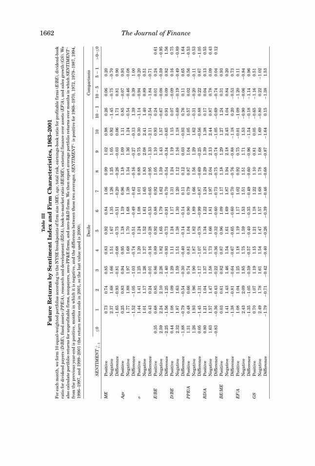
Table III looks for conditional characteristics effects in a simple, nonpara-metric way. We place each monthly return observation into a bin according tothe decile rank that a characteristic takes at the beginning of that month, andthen according to the level of SENTIMENT⊥ at the end of the previous calen-dar year. To keep the meaning of the deciles similar over time, we define thembased on NYSE firms. The trade-off is that there is not a uniform distribution offirms across bins in any given month. We compute the equal-weighted averagemonthly return for each bin and look for patterns. In particular, we identifytime-series changes in cross-sectional effects from the conditional difference ofaverage returns across deciles.
The first rows of Table III show the effect of size, as measured by ME, con-ditional on sentiment. These rows reveal that the size effect of Banz (1981)appears in low sentiment periods only. Specifically, Table III shows that whenSENTIMENT⊥ is negative, returns average 2.37% per month for the bottomME decile and 0.92 for the top decile. A similar pattern is apparent when con-ditioning on CEFD (not reported). A link between the size effect and closed-endfund discounts is also noted by Swaminathan (1996). This pattern is consistentwith some long-known results. Namely, the size effect is essentially a Januaryeffect (Keim (1983), Blume and Stambaugh (1983)), and the January effect, inturn, is stronger after a period of low returns (Reinganum (1983)), which is alsowhen sentiment is likely to be low.
As an aside, note that the average returns across the first two rows of Table IIIillustrate that subsequent returns tend to be higher, across most of the cross-section, when sentiment is low. This is consistent with prior results that theequity share and turnover, for example, forecast market returns. More gen-erally, it supports our premise that sentiment has broad effects, and so theexistence of richer patterns within the cross-section is not surprising.
The conditional cross-sectional effect of Age is striking. In general, in-vestors appear to demand young stocks when SENTIMENT⊥ is positive andprefer older stocks when sentiment is negative. For example, when senti-ment is pessimistic, top-decile Age firms return 0.54% per month less thanbottom-decile Age firms. However, they return 0.85% more when sentimentis optimistic. When sentiment is positive, the effect is concentrated in thevery youngest stocks, which are recent IPOs; when it is negative, the con-trast is between the bottom and top several deciles of age. Overall, there isa nearly monotonic effect in the conditional difference of returns. This re-sult is intriguing because Age has no unconditional effect.10 The strong con-ditional effects, of opposite sign, average out across high and low sentimentperiods.
10 This conclusion is in seeming contrast to Barry and Brown’s (1984) evidence of an uncondi-
tional negative period-of-listing effect; however, their sample excludes stocks listed for fewer than
61 months.
1662 The Journal of FinanceT
able
III
Fu
ture
Ret
urn
sb
yS
enti
men
tIn
dex
and
Fir
mC
har
acte
rist
ics,
1963
–200
1F
or
ea
chm
on
th,w
efo
rm1
0eq
ua
l-w
eig
hte
dp
ort
foli
os
acc
ord
ing
toth
eN
YS
Eb
rea
kp
oin
tsoffi
rmsi
ze(M
E),
age,
tota
lri
sk,ea
rnin
gs-
book
rati
ofo
rp
rofi
tab
lefi
rms
(E/B
E),
div
iden
d-b
ook
rati
ofo
rd
ivid
en
dp
ayers
(D/B
E),
fixed
ass
ets
(PP
E/A
),re
sea
rch
an
dd
evelo
pm
en
t(R
D/A
),b
ook
-to-m
ark
et
rati
o(B
E/M
E),
exte
rna
lfi
na
nce
over
ass
ets
(EF
/A),
an
dsa
les
gro
wth
(GS
).W
e
als
oca
lcu
late
port
foli
ore
turn
sfo
ru
np
rofi
tab
lefi
rms,
non
payers
,ze
ro-P
P&
Efi
rms,
an
dze
ro-R
&D
firm
s.W
eth
en
rep
ort
avera
ge
port
foli
ore
turn
sover
mon
ths
inw
hic
hS
EN
TIM
EN
T⊥
from
the
pre
vio
us
yea
r-en
dis
posi
tive,m
on
ths
inw
hic
hit
isn
ega
tive,a
nd
the
dif
fere
nce
betw
een
these
two
avera
ges.
SE
NT
IME
NT
⊥is
posi
tive
for
19
68
–1
97
0,1
97
2,1
97
9–
19
87
,1
99
4,
19
96
–1
99
7,
an
d1
99
9–
20
01
(th
ere
turn
seri
es
en
ds
in2
00
1,
soth
ela
stva
lue
use
dis
20
00
).
Deci
leC
om
pa
riso
ns
SE
NT
IME
NT
⊥ t−1
≤01
23
45
67
89
10
10
−1
10
−5
5−
1>
0–≤0
ME
Posi
tive
0.7
30
.74
0.8
50
.83
0.9
20
.84
1.0
60
.99
1.0
20
.98
0.2
60
.06
0.2
0
Nega
tive
2.3
71
.68
1.6
61
.51
1.6
71
.35
1.2
61
.25
1.0
50
.92
−1.4
5−0
.75
−0.7
0
Dif
fere
nce
−1.6
5−0
.93
−0.8
1−0
.68
−0.7
5−0
.51
−0.2
0−0
.26
−0.0
30
.06
1.7
10
.81
0.9
0
Age
Posi
tive
0.2
50
.83
0.9
40
.95
1.1
81
.19
0.9
61
.18
1.0
91
.11
0.8
5−0
.07
0.9
3
Nega
tive
1.7
71
.88
1.9
71
.68
1.7
01
.68
1.3
81
.34
1.3
61
.24
−0.5
4−0
.46
−0.0
8
Dif
fere
nce
−1.5
2−1
.05
−1.0
3−0
.74
−0.5
1−0
.49
−0.4
2−0
.16
−0.2
7−0
.13
1.3
90
.39
1.0
0
σP
osi
tive
1.4
41
.41
1.2
51
.20
1.2
41
.08
1.0
10
.88
0.7
50
.30
−1.1
4−0
.94
−0.2
0
Nega
tive
1.0
11
.17
1.2
61
.37
1.5
21
.61
1.6
51
.83
2.0
82
.41
1.4
00
.89
0.5
1
Dif
fere
nce
0.4
30
.24
−0.0
1−0
.16
−0.2
8−0
.53
−0.6
5−0
.95
−1.3
3−2
.11
−2.5
4−1
.84
−0.7
1
E/B
EP
osi
tive
0.3
50
.68
0.8
50
.86
0.8
90
.92
0.8
80
.92
1.0
51
.10
0.9
30
.24
0.0
10
.24
0.6
1
Nega
tive
2.5
92
.24
2.1
02
.26
1.8
21
.65
1.7
91
.62
1.5
91
.43
1.5
7−0
.67
−0.0
8−0
.59
−0.9
5
Dif
fere
nce
−2.2
5−1
.56
−1.2
5−1
.40
−0.9
3−0
.73
−0.9
1−0
.70
−0.5
4−0
.34
−0.6
50
.91
0.0
90
.82
1.5
6
D/B
EP
osi
tive
0.4
41
.08
1.0
91
.29
1.1
11
.24
1.1
71
.31
1.2
41
.19
1.1
50
.07
−0.0
90
.16
0.7
5
Nega
tive
2.3
21
.87
1.6
31
.59
1.5
11
.38
1.3
01
.20
1.1
21
.16
1.1
8−0
.69
−0.1
9−0
.49
−0.8
9
Dif
fere
nce
−1.8
8−0
.79
−0.5
4−0
.30
−0.4
0−0
.14
−0.1
40
.11
0.1
20
.03
−0.0
30
.76
0.1
10
.65
1.6
4
PP
E/A
Posi
tive
1.3
10
.48
0.6
60
.74
0.8
11
.04
0.9
00
.79
0.8
71
.04
1.0
50
.57
0.0
20
.56
−0.5
3
Nega
tive
1.2
61
.93
1.9
61
.90
1.8
71
.82
1.8
91
.66
1.5
61
.29
1.6
2−0
.31
−0.2
0−0
.11
0.5
3
Dif
fere
nce
0.0
5−1
.45
−1.3
1−1
.17
−1.0
7−0
.78
−0.9
9−0
.87
−0.6
9−0
.25
−0.5
60
.88
0.2
20
.67
−1.0
5
RD
/AP
osi
tive
0.8
01
.21
1.0
41
.37
1.3
71
.34
1.2
21
.24
1.2
91
.39
1.3
80
.17
0.0
40
.13
0.5
5
Nega
tive
1.6
31
.57
1.4
71
.58
1.7
31
.66
1.8
11
.97
2.0
42
.13
2.4
40
.87
0.7
80
.09
0.4
3
Dif
fere
nce
−0.8
3−0
.36
−0.4
3−0
.22
−0.3
6−0
.32
−0.6
0−0
.73
−0.7
5−0
.74
−1.0
5−0
.69
−0.7
40
.04
0.1
2
BE
/ME
Posi
tive
0.0
30
.61
0.8
20
.87
0.9
61
.09
1.1
71
.18
1.2
91
.27
1.2
40
.31
0.9
3
Nega
tive
1.4
11
.43
1.4
61
.54
1.6
11
.69
1.8
71
.94
2.1
82
.45
1.0
40
.84
0.2
0
Dif
fere
nce
−1.3
8−0
.81
−0.6
4−0
.67
−0.6
5−0
.60
−0.7
0−0
.76
−0.8
8−1
.18
0.2
0−0
.53
0.7
3
EF
/AP
osi
tive
1.0
81
.04
1.2
51
.18
1.1
91
.17
1.0
20
.92
0.7
5−0
.01
−1.0
9−1
.20
0.1
1
Nega
tive
2.4
32
.09
1.8
51
.75
1.5
91
.53
1.5
11
.51
1.7
11
.53
−0.9
0−0
.06
−0.8
4
Dif
fere
nce
−1.3
5−1
.05
−0.5
9−0
.57
−0.4
0−0
.35
−0.4
9−0
.60
−0.9
6−1
.54
−0.1
8−1
.14
0.9
6
GS
Posi
tive
0.7
01
.07
1.1
91
.15
1.2
11
.18
1.2
21
.10
0.8
10
.05
−0.6
5−1
.16
0.5
1
Nega
tive
2.4
91
.78
1.6
11
.54
1.4
71
.57
1.6
81
.78
1.6
81
.69
−0.8
00
.22
−1.0
2
Dif
fere
nce
−1.7
9−0
.71
−0.4
2−0
.40
−0.2
6−0
.39
−0.4
6−0
.68
−0.8
7−1
.64
0.1
5−1
.38
1.5
3
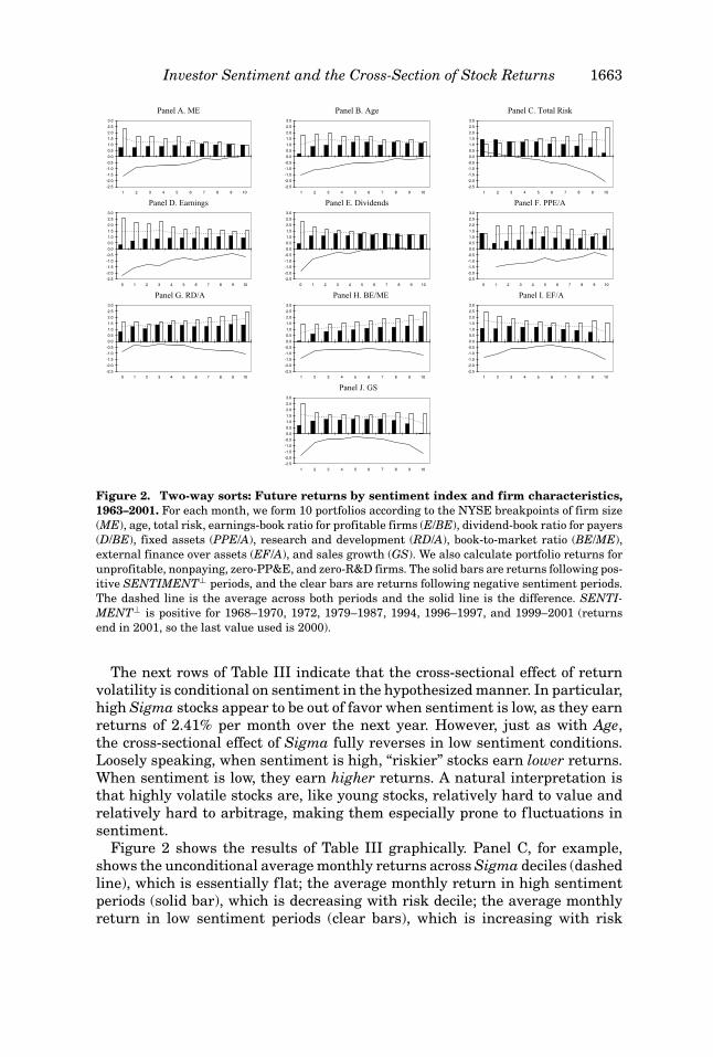
Investor Sentiment and the Cross-Section of Stock Returns 1663
Panel A. ME
-2.5
-2.0
-1.5
-1.0
-0.5
0.0
0.5
1.0
1.5
2.0
2.5
3.0
1 2 3 4 5 6 7 8 9 10
1
Panel B. Age
-2.5
-2.0
-1.5
-1.0
-0.5
0.0
0.5
1.0
1.5
2.0
2.5
3.0
1 2 3 4 5 6 7 8 9 10
Panel C. Total Risk
-2.5
-2.0
-1.5
-1.0
-0.5
0.0
0.5
1.0
1.5
2.0
2.5
3.0
1 2 3 4 5 6 7 8 9 10
Panel D. Earnings
-2.5
-2.0
-1.5
-1.0
-0.5
0.0
0.5
1.0
1.5
2.0
2.5
3.0
0 1 2 3 4 5 6 7 8 9 10
Panel E. Dividends
-2.5
-2.0
-1.5
-1.0
-0.5
0.0
0.5
1.0
1.5
2.0
2.5
3.0
0 1 2 3 4 5 6 7 8 9 10
Panel F. PPE/A
-2.5
-2.0
-1.5
-1.0
-0.5
0.0
0.5
1.0
1.5
2.0
2.5
3.0
0 1 2 3 4 5 6 7 8 9 10
Panel G. RD/A
-2.5
-2.0
-1.5
-1.0
-0.5
0.0
0.5
1.0
1.5
2.0
2.5
3.0
0 1 2 3 4 5 6 7 8 9 10
Panel H. BE/ME
-2.5
-2.0
-1.5
-1.0
-0.5
0.0
0.5
1.0
1.5
2.0
2.5
3.0
1 2 3 4 5 6 7 8 9 10
Panel I. EF/A
-2.5
-2.0
-1.5
-1.0
-0.5
0.0
0.5
1.0
1.5
2.0
2.5
3.0
1 2 3 4 5 6 7 8 9 10
Panel J. GS
-2.5
-2.0
-1.5
-1.0
-0.5
0.0
0.5
1.0
1.5
2.0
2.5
3.0
1 2 3 4 5 6 7 8 9 10
Figure 2. Two-way sorts: Future returns by sentiment index and firm characteristics,1963–2001. For each month, we form 10 portfolios according to the NYSE breakpoints of firm size
(ME), age, total risk, earnings-book ratio for profitable firms (E/BE), dividend-book ratio for payers
(D/BE), fixed assets (PPE/A), research and development (RD/A), book-to-market ratio (BE/ME),
external finance over assets (EF/A), and sales growth (GS). We also calculate portfolio returns for
unprofitable, nonpaying, zero-PP&E, and zero-R&D firms. The solid bars are returns following pos-
itive SENTIMENT⊥ periods, and the clear bars are returns following negative sentiment periods.
The dashed line is the average across both periods and the solid line is the difference. SENTI-MENT⊥ is positive for 1968–1970, 1972, 1979–1987, 1994, 1996–1997, and 1999–2001 (returns
end in 2001, so the last value used is 2000).
The next rows of Table III indicate that the cross-sectional effect of returnvolatility is conditional on sentiment in the hypothesized manner. In particular,high Sigma stocks appear to be out of favor when sentiment is low, as they earnreturns of 2.41% per month over the next year. However, just as with Age,the cross-sectional effect of Sigma fully reverses in low sentiment conditions.Loosely speaking, when sentiment is high, “riskier” stocks earn lower returns.When sentiment is low, they earn higher returns. A natural interpretation isthat highly volatile stocks are, like young stocks, relatively hard to value andrelatively hard to arbitrage, making them especially prone to fluctuations insentiment.
Figure 2 shows the results of Table III graphically. Panel C, for example,shows the unconditional average monthly returns across Sigma deciles (dashedline), which is essentially flat; the average monthly return in high sentimentperiods (solid bar), which is decreasing with risk decile; the average monthlyreturn in low sentiment periods (clear bars), which is increasing with risk

1664 The Journal of Finance
deciles; and the difference in conditional returns (solid line). The solid linesummarizes the difference in the relationship between Sigma and future re-turns across the two regimes and clearly illustrates that the future returns onhigh Sigma stocks are more sensitive to sentiment.
The next rows examine profitability and dividends. For average investors,perhaps the most salient comparisons are simply those between profitable andunprofitable (E < 0) firms and payers and nonpayers (D = 0). These contrastsare in the extreme right column, where we average returns across profitable(paying) firms and compare them to unprofitable (nonpaying) firms. Thesecharacteristics again display intriguing conditional sign-flip patterns. Whensentiment is positive, monthly returns over the next year are 0.61% higher onprofitable than unprofitable firms and 0.75% higher on payers than nonpayers.When it is negative, however, returns are 0.95% per month lower on profitablefirms and 0.89% lower on payers. The left column shows that these patternsare driven mostly by conditional variation in the returns of unprofitable andnonpaying firms, although there are also some differences across levels of div-idend payments and profitability. Again, this is consistent with unprofitable,nonpaying firms being generally harder both to value and to arbitrage, thusexposing them more to sentiment fluctuations.
The next two rows look at asset tangibility characteristics under the notionthat firms with less tangible assets may be more difficult to value. The patternshere are not so strong, but there is a suggestion that firms with more intangibleassets, as measured by less PPE/A, are more sensitive to fluctuations in senti-ment. (This pattern is only apparent within firms that report positive PPE/A.)The clearest pattern in RD/A is a modest unconditional effect in which higherRD/A firms earn higher returns.
The remaining variables—book-to-market, external finance, and salesgrowth—also display intriguing patterns. Most simply, running across rows,one can see that each of them has some unconditional explanatory power. Fu-ture returns are generally higher for high BE/ME stocks, low EF/A stocks, andlow GS decile stocks. The EF/A result is reminiscent of Loughran and Ritter(1995) and Spiess and Affleck-Graves (1995, 1999), while the GS result is sug-gested in Lakonishok, Shleifer, and Vishny (1994).
A closer look reveals that after controlling for these unconditional effects, aconditional pattern emerges. Specifically, there is a U-shaped pattern in theconditional difference. Consider the GS variable. The difference in returns onbottom-decile GS firms is −1.79% per month. For fifth-decile firms, the differ-ence is only −0.26% per month. But for tenth-decile firms, the difference isagain large, −1.64% per month. U-shaped patterns also appear in the condi-tional difference row for BE/ME and EF/A. The solid lines in Panels H–J ofFigure 2 show these “frowns” graphically. The figure illustrates why one mustcontrol for the strong unconditional effects in these variables in order to see theconditional effects.
Thus, in all three of these growth and distress variables, firms with extremevalues react more to sentiment than firms with middle values. What does

Investor Sentiment and the Cross-Section of Stock Returns 1665
the U reflect? It reflects the multidimensional nature of the growth and dis-tress variables. Consider GS. High-GS firms include high-flying growth firms,low-GS firms are often distressed firms with shrinking sales, and middle-GSfirms are steady, slow-growth firms. Thus, relative to firms in the middle deciles,firms with extreme values of GS are harder to value, and perhaps to arbitrage,and thus may be more sensitive to sentiment. Put differently, firms with ex-treme values of GS are likely to seem riskier, in a salient sense, than firmsin the middle. The same explanation may help to explain the U-shaped pat-terns in the conditional difference row of EF/A and BE/ME. There again, lowEF/A firms and high BE/ME firms include distressed firms, high EF/A and lowBE/ME firms include high-flyers, and the middle deciles tend to be populatedby the most “stable” firms.
In unreported results, we sort returns not just on positive and negative valuesof SENTIMENT⊥ but also on >1 and <−1 standard deviation values. Not sur-prisingly, conditioning on more extreme values of sentiment leads to strongerresults. We take more formal account of the continuous nature of the sentimentindexes in the next subsection. Also, for brevity, we omit sorts on SENTIMENT(the nonorthogonalized version), which give similar results. We present resultsfor both indexes in the next section. Finally, we have also sorted returns onpositive and negative SENTIMENT⊥, where positive and negative are definedrelative to a 10-year average. By requiring a 10-year history of sentiment, oneloses a little more than one-quarter of the sample. The results are qualitativelyidentical to those in Table III, although slightly weaker except for Age, whichis slightly stronger.
B. Predictive Regressions for Long–Short Portfolios
Another way to look for conditional characteristics effects is to use sentimentto forecast equal-weighted portfolios that are long on stocks with high values ofa characteristic and short on stocks with low values. Above we see that the aver-age payer, for example, earns higher returns than the average nonpayer whensentiment is high, so sentiment seems likely to forecast a long–short portfolioformed on dividend payment. But a regression approach allows us to conductformal significance tests, incorporate the continuous nature of the sentimentindexes, and determine which characteristics have conditional effects that aredistinct from well-known unconditional effects.
Table IV starts by plotting the average monthly returns on various long–shortportfolios over time. The first several rows show that, not surprisingly, long–short portfolios formed on size (SMB), age, volatility, profitability, dividendpayment, and (to a lesser extent) tangibility are typically highly correlated.Thus, a good question, which we address in subsequent tables, is whether theresults from the sorts are all part of the same pattern or are somewhat distinct.This question is also relevant given that our portfolios are equal-weighted. Bycontrolling for SMB in portfolio forecasting regressions, we can examine theextent to which the conditional predictability patterns are independent of size.
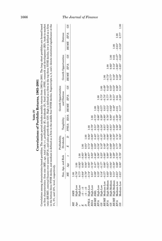
1666 The Journal of Finance
Tab
leIV
Cor
rela
tion
sof
Por
tfol
ioR
etu
rns,
1963
–200
1C
orr
ela
tion
sa
mon
gch
ara
cteri
stic
s-b
ase
dp
ort
foli
os.
Th
esa
mp
lep
eri
od
incl
ud
es
mon
thly
retu
rns
from
19
63
to2
00
1.T
he
lon
g–
short
port
foli
os
are
form
ed
ba
sed
on
firm
cha
ract
eri
stic
s:fi
rmsi
ze(M
E),
age,
tota
lri
sk(σ
),p
rofi
tab
ilit
y(E
),d
ivid
en
ds
(D),
fixed
ass
ets
(PP
E),
rese
arc
han
dd
evelo
pm
en
t(R
D),
book
-to-m
ark
et
rati
o(B
E/M
E),
exte
rna
lfi
na
nce
over
ass
ets
(EF
/A),
an
dsa
les
gro
wth
deci
le(G
S).
Hig
his
defi
ned
as
afi
rmin
the
top
thre
eN
YS
Ed
eci
les,
low
isd
efi
ned
as
afi
rm
inth
eb
ott
om
thre
eN
YS
Ed
eci
les,
an
dm
ed
ium
isd
efi
ned
as
afi
rmin
the
mid
dle
fou
rN
YS
Ed
eci
les.
Su
pers
crip
tsa,b,an
dc
den
ote
sta
tist
ica
lsi
gn
ific
an
ceat
the
1%
,5
%,a
nd
10
%,le
vel,
resp
ect
ively
.
Pro
fita
bil
ity,
Gro
wth
Op
port
un
itie
s
Siz
e,A
ge,an
dR
isk
Div
iden
ds
Tan
gib
ilit
ya
nd
Dis
tress
Gro
wth
Op
port
un
itie
sD
istr
ess
ME
Age
σE
DP
PE
/AR
D/A
BE
/ME
EF
/AG
SB
E/M
EE
F/A
GS
BE
/ME
EF
/AG
S
ME
SM
B1
.00
Age
Hig
h-L
ow
−0.7
8a
1.0
0
σH
igh
-Low
0.7
7a
−0.9
2a
1.0
0
E>
0–
<0
−0.6
4a
0.8
5a
−0.8
5a
1.0
0
D>
0–
=0−0
.76
a0
.94
a−0
.96
a0
.91
a1
.00
PP
E/A
Hig
h-L
ow
−0.7
4a
0.8
5a
−0.8
7a
0.7
1a
0.8
4a
1.0
0
RD
/AH
igh
-Low
0.6
1a
−0.7
8a
0.8
2a
−0.6
9a
−0.8
0a
−0.7
9a
1.0
0
BE
/ME
HM
L0
.09
a0
.47
a−0
.46
a0
.23
a0
.43
a0
.51
a−0
.73
a1
.00
EF
/AH
igh
-Low
0.3
3a
−0.5
5a
0.5
6a
−0.3
4a
−0.5
1a
−0.5
9a
0.6
6a
−0.6
5a
1.0
0
GS
Hig
h-L
ow
0.1
4a
−0.1
7a
0.2
3a
0.1
0b
−0.1
5a
−0.3
4a
0.2
9a
−0.5
7a
0.7
3a
1.0
0
BE
/ME
Med
ium
-Low
−0.3
7a
0.6
6a
−0.6
8a
0.4
8a
0.6
4a
0.6
1a
−0.8
0a
0.8
1a
−0.7
4a
−0.4
9a
1.0
0
EF
/AH
igh
-Med
ium
0.6
5a
−0.8
7a
0.9
0a
−0.7
6a
−0.8
8a
−0.8
3a
0.7
6a
−0.5
1a
0.7
7a
0.4
2a
−0.7
3a
1.0
0
GS
Hig
h-M
ed
ium
0.6
5a
−0.8
4a
0.8
8a
−0.6
9a
−0.8
6a
−0.8
1a
0.8
0a
−0.6
2a
0.7
8a
0.5
5a
−0.7
7a
0.9
2a
1.0
0
BE
/ME
Hig
h-M
ed
ium
0.3
1a
−0.3
0a
0.2
9a
−0.5
0a
−0.3
5a
−0.2
2a
−0.0
10
.40
a−0
.31
a−0
.53
a0
.16
a0
.14
a0
.03
1.0
0
EF
/AM
ed
ium
-Low
−0.6
1a
0.6
9a
−0.7
0a
0.7
7a
0.7
4a
0.5
6a
−0.3
9a
−0.0
10
.04
0.2
6a
0.2
3a
−0.6
0a
−0.4
7a
−0.6
1a
1.0
0
GS
Med
ium
-Low
−0.6
1a
0.8
0a
−0.7
9a
0.8
8a
0.8
3a
0.6
0a
−0.6
2a
0.1
7a
−0.2
0a
0.3
1a
0.4
2a
−0.6
5a
−0.6
3a
−0.5
3a
0.7
7a
1.0
0

Investor Sentiment and the Cross-Section of Stock Returns 1667
In the last several rows of Table IV, we break the growth and distress vari-ables into “high minus medium” and “medium minus low” portfolios. In the caseof the GS variable, for example, these portfolios are highly negatively correlatedwith each other, at −0.63, indicating that high and low GS firms actually movetogether relative to middle GS firms. Likewise, the correlation between “highminus medium” and “medium minus low” EF/A is −0.60. Thus, simple “highminus low” analyses of these variables would omit crucial aspects of the cross-section.
The question is whether sentiment can predict the various long–short port-folios analyzed in Table IV. We run regressions of the type11
RX it=High,t − RX it=Low,t = c + dSENTIMENTt−1 + uit. (4)
The dependent variable is the monthly return on a long–short portfolio, suchas SMB, and the monthly returns from January through December of t areregressed on the sentiment index that prevailed at the end of the prior year.We also distinguish novel predictability effects from well-known comovementusing the multivariate regression
RX it=High,t − RX it=Low,t = c + dSENTIMENTt−1 + βRMKTt + sSMBt
+ hHMLt + mUMDt + uit. (5)
The variable RMRF is the excess return of the value-weighted market overthe risk-free rate. The variable UMD is the return on high-momentum stocksminus the return on low-momentum stocks, where momentum is measuredover months [−12, −2]. As described in Fama and French (1993), SMB is thereturn on portfolios of small and big ME stocks that is separate from returns onHML, where HML is constructed to isolate the difference between high and lowBE/ME portfolios.12 We exclude SMB and HML from the right side when theyare the portfolios being forecast. Standard errors are bootstrapped to correctfor the bias induced if the autocorrelated sentiment index has innovations thatare correlated with innovations in portfolio returns, as in Stambaugh (1999).
Table V shows the results. The results provide formal support to our pre-liminary impressions from the sorts. In particular, the first panel shows thatwhen sentiment is high, returns on small, young, and high volatility firms arerelatively low over the coming year. The coefficient on sentiment diminishesonce we control for RMRF, SMB, HML, and UMD, but in most cases the signif-icance of the predictive effect does not depend on including or excluding thesecontrols. In terms of magnitudes, the coefficient for predicting SMB, for exam-ple, indicates that a one-unit increase in sentiment (which equals a one-SDincrease, because the indexes are standardized) is associated with a −0.40%lower monthly return on the small minus large portfolio.
11 Intuitively, in terms of equation (1), this amounts to a regression of (b1�X + b2Tt−1�X ) on sen-
timent proxies Tt−1, where �X is the difference between “high” and “low” levels of a characteristic.12 These portfolios are taken from Ken French’s website and are described there.

1668 The Journal of Finance
Table V also shows that the coefficients on SENTIMENT and SENTIMENT⊥
are very similar. Keep in mind that the coefficients on SENTIMENT⊥ are essen-tially the same as one would find from regressing long–short portfolio returnsdirectly on a raw sentiment index and controls for contemporaneous macroeco-nomic conditions—that is, regressing X on Z and using the residuals to predictY is equivalent to regressing Y on X and Z. The similarity of the results onSENTIMENT and SENTIMENT⊥ thus suggests that macroeconomic condi-tions play a minor role.
For profitability and dividend payment, we run regressions to predict thedifference between the profitable and paying portfolios and the unprofitableand nonpaying portfolios, respectively, because the sorts suggest that these arelikely to capture the main contrasts. The results show that sentiment indeedhas significant predictive power for these portfolios, with higher sentiment fore-casting relatively higher returns on payers and profitable firms. The patternsare little affected by controlling for RMRF, SMB, HML, and UMD.
As we find with the sorts, the tangibility characteristics do not exhibit strongconditional effects. Sentiment does have marginal predictive power for thePPE/A portfolio, with high sentiment associated with relatively low future re-turns on low PPE/A stocks, but this disappears after controlling for RMRF,SMB, HML, and UMD. The coefficients on the RD/A portfolio forecasts are notconsistent in sign or magnitude.
Also as we find with the sorts, the “growth and distress” variables do not havesimple monotonic relationships with sentiment. Panel D shows that sentimentdoes not predict simple high minus low portfolios formed on any of BE/ME,EF/A, or GS. However, Panels E and F show that when the multidimensionalnature of these variables is incorporated, there is much stronger evidence ofpredictive power. We separate extreme growth opportunities effects from dis-tress effects by constructing High, Medium, and Low portfolios based on thetop three, middle four, and bottom three NYSE decile breakpoints, respectively.
The results show that when sentiment is high, subsequent returns on bothlow and high sales growth firms are low relative to returns on medium growthfirms. This illustrates the U-shaped pattern in Table III in a different way,and shows that it is statistically significant. An equally significant U-shapedpattern is apparent with external finance; when sentiment is high, subsequentreturns on both low and high external finance firms are low relative to moretypical firms. In the case of BE/ME, however, although sentiment predicts thehigh minus medium and medium minus low portfolios with opposite signs,neither coefficient is reliably significant. This matches our inferences from thesorts, where we see that the U-shaped pattern in the conditional difference forBE/ME is somewhat weaker than for EF/A and GS.
Equations (4) and (5) offer a simple framework in which to address somerobustness issues. To test whether the results are driven by an overall trend,we include a post-1982 dummy in the regressions, with no change in inferencesfrom those in the last column of Table V. Also, the results are slightly strongerwhen returns from January and December are removed from the sample. This

Investor Sentiment and the Cross-Section of Stock Returns 1669
Tab
leV
Tim
eS
erie
sR
egre
ssio
ns
ofP
ortf
olio
Ret
urn
s,19
63to
2001
Regre
ssio
ns
of
lon
g–
short
port
foli
ore
turn
son
lagged
SE
NT
IME
NT
,th
em
ark
et
risk
pre
miu
m(R
MR
F),
the
Fa
ma
–F
ren
chfa
ctors
(HM
La
nd
SM
B),
an
da
mom
en
tum
fact
or
(UM
D).
RX
it=H
igh
,t−
RX
it=L
ow,t
=c
+d
SE
NT
IME
NT
t−1
+β
RM
RF
t+
sSM
Bt+
hH
ML
t+
mU
MD
t+
u t.
Th
esa
mp
lep
eri
od
incl
ud
es
mon
thly
retu
rns
from
19
63
to2
00
1.
Th
elo
ng–
short
port
foli
os
are
form
ed
ba
sed
on
firm
cha
ract
eri
stic
s(X
):fi
rmsi
ze
(ME
),ag
e,to
tal
risk
(σ),
pro
fita
bil
ity
(E),
div
iden
ds
(D),
fixed
ass
ets
(PP
E),
rese
arc
ha
nd
develo
pm
en
t(R
D),
book
-to-m
ark
et
rati
o(B
E/M
E),
exte
rna
l
fin
an
ceover
ass
ets
(EF
/A),
an
dsa
les
gro
wth
deci
le(G
S).
Hig
his
defi
ned
as
afi
rmin
the
top
thre
eN
YS
Ed
eci
les,
low
isd
efi
ned
as
afi
rmin
the
bott
om
thre
eN
YS
Ed
eci
les,
an
dm
ed
ium
isd
efi
ned
as
afi
rmin
the
mid
dle
fou
rN
YS
Ed
eci
les.
Avera
ge
mon
thly
retu
rns
are
ma
tch
ed
toS
EN
TIM
EN
Tfr
om
the
pre
vio
us
yea
r-en
d.S
EN
TIM
EN
T⊥
ind
ex
isb
ase
don
six
sen
tim
en
tp
roxie
sth
at
have
been
ort
hogon
ali
zed
togro
wth
inin
du
stri
al
pro
du
ctio
n,th
e
gro
wth
ind
ura
ble
,non
du
rab
le,a
nd
serv
ices
con
sum
pti
on
,th
egro
wth
inem
plo
ym
en
t,a
nd
afl
ag
for
NB
ER
rece
ssio
ns;
the
com
pon
en
tsofS
EN
TIM
EN
Ta
ren
ot
ort
hogon
ali
zed
.T
he
firs
ta
nd
thir
dse
tsofco
lum
ns
show
un
iva
ria
tere
gre
ssio
nre
sult
s,w
hil
eth
ese
con
da
nd
the
fou
rth
colu
mn
sin
clu
de
RM
RF
,
SM
B,H
ML
,an
dU
MD
as
con
trolva
ria
ble
s.S
MB
(HM
L)is
not
incl
ud
ed
as
aco
ntr
olva
ria
ble
wh
en
SM
B(H
ML
)is
the
dep
en
den
tva
ria
ble
.Boots
tra
pp
ed
p-va
lues
are
inb
rack
ets
.
SE
NT
IME
NT
t −1
SE
NT
IME
NT
⊥ t−1
Con
troll
ing
for
Con
troll
ing
for
RM
RF
,S
MB
,R
MR
F,
SM
B,
SE
NT
IME
NT
t −1
HM
L,
UM
DS
EN
TIM
EN
T⊥ t−
1H
ML
,U
MD
dp
(d)
dp
(d)
dp
(d)
dp
(d)
Pa
nel
A:
Siz
e,
Age,
an
dR
isk
ME
SM
B−0
.4[0
.04
]−0
.3[0
.08
]−0
.4[0
.06
]−0
.3[0
.15
]
Age
Hig
h-L
ow0
.5[0
.02
]0
.2[0
.08
]0
.5[0
.01
]0
.2[0
.04
]
σH
igh
-Low
−1.0
[0.0
1]
−0.5
[0.0
1]
−0.9
[0.0
0]
−0.4
[0.0
1]
Pa
nel
B:
Pro
fita
bil
ity
an
dD
ivid
en
dP
oli
cy
E>
0–<
00
.8[0
.00
]0
.5[0
.02
]0
.8[0
.00
]0
.4[0
.02
]
D>
0–
=0
0.8
[0.0
0]
0.4
[0.0
0]
0.8
[0.0
0]
0.4
[0.0
0]
(con
tin
ued
)
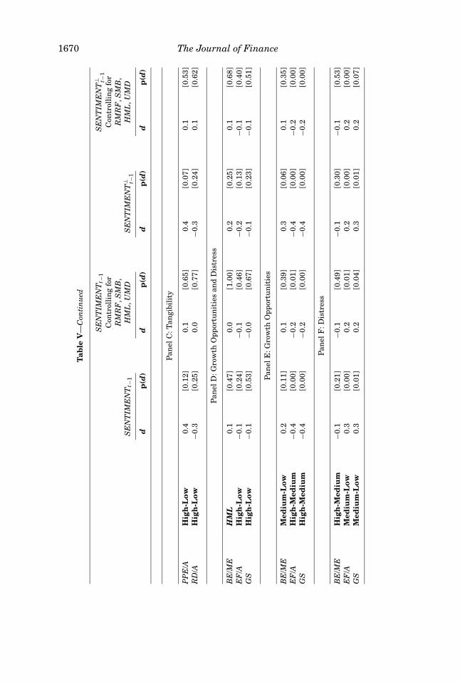
1670 The Journal of Finance
Tab
leV
—C
onti
nu
ed
SE
NT
IME
NT
t −1
SE
NT
IME
NT
⊥ t−1
Con
troll
ing
for
Con
troll
ing
for
RM
RF
,S
MB
,R
MR
F,
SM
B,
SE
NT
IME
NT
t −1
HM
L,
UM
DS
EN
TIM
EN
T⊥ t−
1H
ML
,U
MD
dp
(d)
dp
(d)
dp
(d)
dp
(d)
Pa
nel
C:
Ta
ngib
ilit
y
PP
E/A
Hig
h-L
ow0
.4[0
.12
]0
.1[0
.65
]0
.4[0
.07
]0
.1[0
.53
]
RD
/AH
igh
-Low
−0.3
[0.2
5]
0.0
[0.7
7]
−0.3
[0.2
4]
0.1
[0.6
2]
Pan
el
D:
Gro
wth
Op
port
un
itie
sa
nd
Dis
tress
BE
/ME
HM
L0
.1[0
.47
]0
.0[1
.00
]0
.2[0
.25
]0
.1[0
.68
]
EF
/AH
igh
-Low
−0.1
[0.2
4]
−0.1
[0.4
6]
−0.2
[0.1
3]
−0.1
[0.4
0]
GS
Hig
h-L
ow−0
.1[0
.53
]−0
.0[0
.67
]−0
.1[0
.23
]−0
.1[0
.51
]
Pa
nel
E:
Gro
wth
Op
port
un
itie
s
BE
/ME
Med
ium
-Low
0.2
[0.1
1]
0.1
[0.3
9]
0.3
[0.0
6]
0.1
[0.3
5]
EF
/AH
igh
-Med
ium
−0.4
[0.0
0]
−0.2
[0.0
1]
−0.4
[0.0
0]
−0.2
[0.0
0]
GS
Hig
h-M
ediu
m−0
.4[0
.00
]−0
.2[0
.00
]−0
.4[0
.00
]−0
.2[0
.00
]
Pa
nel
F:
Dis
tress
BE
/ME
Hig
h-M
ediu
m−0
.1[0
.21
]−0
.1[0
.49
]−0
.1[0
.30
]−0
.1[0
.53
]
EF
/AM
ediu
m-L
ow0
.3[0
.00
]0
.2[0
.01
]0
.2[0
.00
]0
.2[0
.00
]
GS
Med
ium
-Low
0.3
[0.0
1]
0.2
[0.0
4]
0.3
[0.0
1]
0.2
[0.0
7]

Investor Sentiment and the Cross-Section of Stock Returns 1671
indicates that tax-motivated trading and associated fluctuations in liquidityaround the turn of the year do not drive the main results. Further, our port-folios are equal-weighted. As mentioned previously, the purpose of this is thattheory predicts that small firms will be most affected by sentiment, and hencevalue weighting will obscure the relevant patterns. Yet by sorting on charac-teristics that are correlated with size, as several of our characteristics are, andthen equal-weighting these characteristics portfolios, one worries that we arejust picking up the size effect once again. By controlling for SMB in portfolioforecasting regressions, we can see that several of the conditional predictabilitypatterns are distinguishable from size, though as theory predicts the predictivecoefficient is attenuated. Finally, while we omit the results for brevity, the sixindividual sentiment components generally predict the portfolio returns withthe expected sign. The number of IPOs and the closed-end fund discount offerthe best individual performance, followed by the equity share, turnover, the av-erage first-day return, and the dividend premium. (Those results are reportedin the NBER working paper version of this paper.)
In summary, the regressions essentially confirm the significance of the pat-terns suggested in the sorts. When sentiment is high, future returns are rela-tively low for small firms, the youngest firms, firms with volatile stock returns,unprofitable firms, non-dividend-paying firms, high growth firms, and dis-tressed firms. And vice-versa. In general, the results support predictions thatsentiment has stronger effects on stocks that are hard to value and hard toarbitrage.
C. A Brief Look at Earlier Data
Reliable accounting information, especially on the sorts of firms most affectedby sentiment, is not easy to obtain for the pre-Compustat era. Some of oursentiment proxies also are not available. However, using CRSP data, we canperform a reduced set of tests over a longer period. Specifically, we form asentiment index from 1935 to 2001 using the first principal component of CEFD,S, and TURN, where TURN is lagged relative to the others, in the spirit ofequation (2).13 We also orthogonalize these sentiment proxies with respect toconsumption growth variables and NBER recessions (industrial production isnot available over the full period) to form an index in the spirit of equation (3).We use these indexes to forecast the return on SMB and long–short portfoliosformed on Age, Sigma, and dividend payer status.
The results are in Table VI. With the exception of the Age portfolio, forwhich the results are not significant, the results from the full 1935–2001 pe-riod and the “out-of-sample” 1935–1961 period are similar to those in more
13 The closed-end fund discount is first available in 1933 from Neal and Wheatley (1998):
“Wiesenberger’s survey has published end-of-year fund prices and net asset values since 1943.
Moreover, the first edition of the survey contains end-of-year data from 1933 to 1942.” Turnover
and the equity share in new issues are available in earlier years. None of our inferences in Panel
A of Table VI change when we use a longer sample period and a sentiment index based on these
two variables alone.
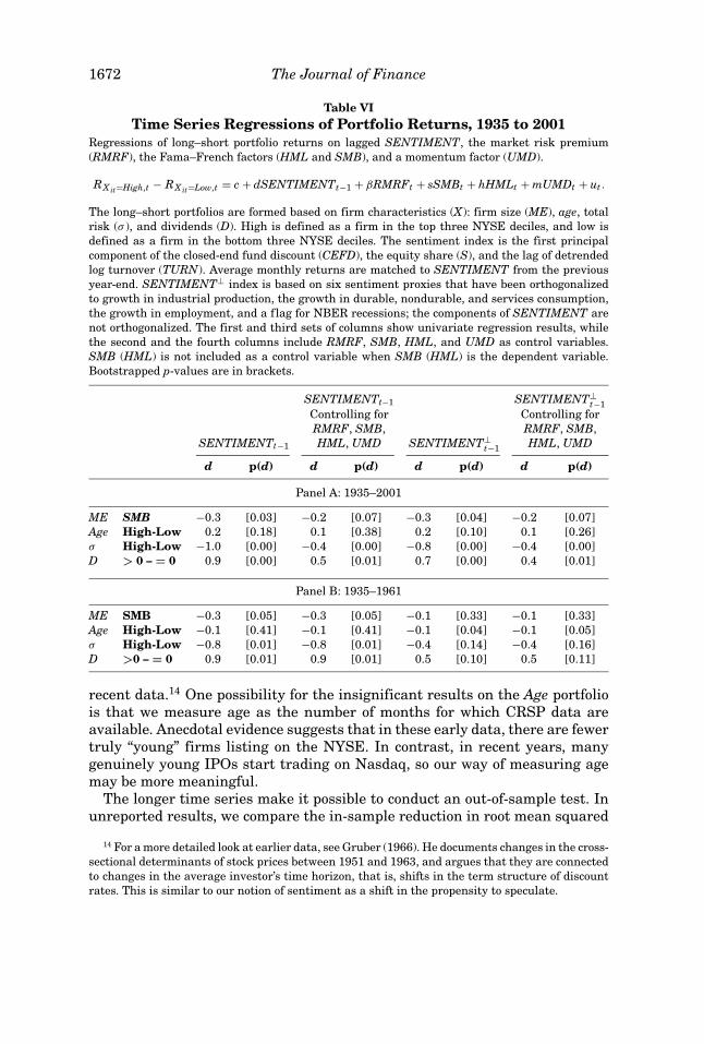
1672 The Journal of Finance
Table VITime Series Regressions of Portfolio Returns, 1935 to 2001
Regressions of long–short portfolio returns on lagged SENTIMENT, the market risk premium
(RMRF), the Fama–French factors (HML and SMB), and a momentum factor (UMD).
RX it=High,t − RX it=Low,t = c + dSENTIMENTt−1 + βRMRFt + sSMBt + hHMLt + mUMDt + ut .
The long–short portfolios are formed based on firm characteristics (X): firm size (ME), age, total
risk (σ ), and dividends (D). High is defined as a firm in the top three NYSE deciles, and low is
defined as a firm in the bottom three NYSE deciles. The sentiment index is the first principal
component of the closed-end fund discount (CEFD), the equity share (S), and the lag of detrended
log turnover (TURN). Average monthly returns are matched to SENTIMENT from the previous
year-end. SENTIMENT⊥ index is based on six sentiment proxies that have been orthogonalized
to growth in industrial production, the growth in durable, nondurable, and services consumption,
the growth in employment, and a flag for NBER recessions; the components of SENTIMENT are
not orthogonalized. The first and third sets of columns show univariate regression results, while
the second and the fourth columns include RMRF, SMB, HML, and UMD as control variables.
SMB (HML) is not included as a control variable when SMB (HML) is the dependent variable.
Bootstrapped p-values are in brackets.
SENTIMENTt−1 SENTIMENT⊥t−1
Controlling for Controlling for
RMRF, SMB, RMRF, SMB,
SENTIMENTt−1 HML, UMD SENTIMENT⊥t−1
HML, UMD
d p(d) d p(d) d p(d) d p(d)
Panel A: 1935–2001
ME SMB −0.3 [0.03] −0.2 [0.07] −0.3 [0.04] −0.2 [0.07]
Age High-Low 0.2 [0.18] 0.1 [0.38] 0.2 [0.10] 0.1 [0.26]
σ High-Low −1.0 [0.00] −0.4 [0.00] −0.8 [0.00] −0.4 [0.00]
D > 0 – = 0 0.9 [0.00] 0.5 [0.01] 0.7 [0.00] 0.4 [0.01]
Panel B: 1935–1961
ME SMB −0.3 [0.05] −0.3 [0.05] −0.1 [0.33] −0.1 [0.33]
Age High-Low −0.1 [0.41] −0.1 [0.41] −0.1 [0.04] −0.1 [0.05]
σ High-Low −0.8 [0.01] −0.8 [0.01] −0.4 [0.14] −0.4 [0.16]
D >0 – = 0 0.9 [0.01] 0.9 [0.01] 0.5 [0.10] 0.5 [0.11]
recent data.14 One possibility for the insignificant results on the Age portfoliois that we measure age as the number of months for which CRSP data areavailable. Anecdotal evidence suggests that in these early data, there are fewertruly “young” firms listing on the NYSE. In contrast, in recent years, manygenuinely young IPOs start trading on Nasdaq, so our way of measuring agemay be more meaningful.
The longer time series make it possible to conduct an out-of-sample test. Inunreported results, we compare the in-sample reduction in root mean squared
14 For a more detailed look at earlier data, see Gruber (1966). He documents changes in the cross-
sectional determinants of stock prices between 1951 and 1963, and argues that they are connected
to changes in the average investor’s time horizon, that is, shifts in the term structure of discount
rates. This is similar to our notion of sentiment as a shift in the propensity to speculate.

Investor Sentiment and the Cross-Section of Stock Returns 1673
error (RMSE) in Table VI to the reduction in RMSE that an investor mightsee using only past data. The results suggest that a substantial fraction of theportfolio predictability would have been “knowable” in advance. The exceptionsare the Age portfolio and the SMB portfolio in the post-1980 period (for whichthe in-sample predictive power for SMB is also modest). A table is available onrequest.
Together, the longer-sample results and the out-of-sample exercise rule outthe possibility that a spurious correlation is behind the main results. The factthat there are at least several fluctuations in sentiment, and the fact that thecross-sectional patterns tend to work in the predicted directions, cast furtherdoubt on that notion.
D. Systematic Risk
At face value, the conditional characteristics effects seem unlikely to becompensation for systematic risk. Among other considerations, the indexSENTIMENT⊥ is orthogonalized to macroeconomic conditions; the patternsmatch predictions about where sentiment should matter most; and the patternsline up with anecdotal accounts of bubbles and crashes. Intuitively, the sys-tematic risk explanation requires that older, profitable, less volatile, dividend-paying firms often require higher returns than younger, unprofitable, morevolatile, nonpaying firms, and are recognized as riskier in the relevant sense bythe marginal investor. While this proposition already seems counterintuitive,we attempt to rule it out more rigorously.
Systematic risk explanations come in two basic flavors. One is that the sys-tematic risks (beta loadings) of stocks with certain characteristics vary withthe sentiment proxies, despite our effort to isolate them from macroeconomicconditions. We investigate this directly in Table VII, where we ask whethersentiment coincides with time-variation in market betas in a way that couldat least qualitatively reconcile the earlier results with a conditional CAPM.Specifically, we predict returns on the characteristics portfolios
RX it=High,t − RX it=Low,t = c + dSENTIMENTt−1
+ β(e + fSENTIMENTt−1)RMRFt + uit. (6)
The time-varying betas story predicts that the composite coefficient βf , reportedin Table VII, has the same sign as the estimates of d in Table V. However, it turnsout that when the coefficient βf is significant, it is typically of the wrong sign.We obtain similar results when we replace RMRF by aggregate consumptiongrowth. A table is available upon request.
The second systematic risk story keeps stocks’ betas fixed, but allows the riskpremium to vary with sentiment, which means that the difference in requiredreturns between the high and low beta stocks varies in proportion. However,this story runs into trouble with the simple fact that the predicted effect ofseveral characteristics varies not just in magnitude over time, but also in sign.It would seem then that the bulk of the results do not reflect compensation forclassical systematic risks.
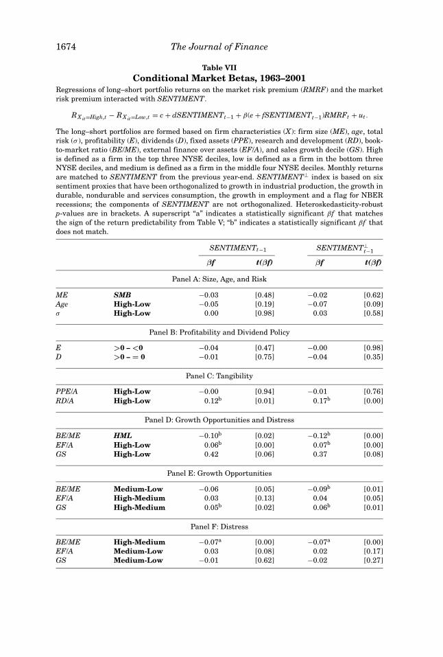
1674 The Journal of Finance
Table VIIConditional Market Betas, 1963–2001
Regressions of long–short portfolio returns on the market risk premium (RMRF) and the market
risk premium interacted with SENTIMENT.
RX it=High,t − RX it=Low,t = c + dSENTIMENTt−1 + β(e + fSENTIMENTt−1)RMRFt + ut .
The long–short portfolios are formed based on firm characteristics (X): firm size (ME), age, total
risk (σ ), profitability (E), dividends (D), fixed assets (PPE), research and development (RD), book-
to-market ratio (BE/ME), external finance over assets (EF/A), and sales growth decile (GS). High
is defined as a firm in the top three NYSE deciles, low is defined as a firm in the bottom three
NYSE deciles, and medium is defined as a firm in the middle four NYSE deciles. Monthly returns
are matched to SENTIMENT from the previous year-end. SENTIMENT⊥ index is based on six
sentiment proxies that have been orthogonalized to growth in industrial production, the growth in
durable, nondurable and services consumption, the growth in employment and a flag for NBER
recessions; the components of SENTIMENT are not orthogonalized. Heteroskedasticity-robust
p-values are in brackets. A superscript “a” indicates a statistically significant βf that matches
the sign of the return predictability from Table V; “b” indicates a statistically significant βf that
does not match.
SENTIMENTt−1 SENTIMENT⊥t−1
βf t(βf) βf t(βf)
Panel A: Size, Age, and Risk
ME SMB −0.03 [0.48] −0.02 [0.62]
Age High-Low −0.05 [0.19] −0.07 [0.09]
σ High-Low 0.00 [0.98] 0.03 [0.58]
Panel B: Profitability and Dividend Policy
E >0 – <0 −0.04 [0.47] −0.00 [0.98]
D >0 – = 0 −0.01 [0.75] −0.04 [0.35]
Panel C: Tangibility
PPE/A High-Low −0.00 [0.94] −0.01 [0.76]
RD/A High-Low 0.12b [0.01] 0.17b [0.00]
Panel D: Growth Opportunities and Distress
BE/ME HML −0.10b [0.02] −0.12b [0.00]
EF/A High-Low 0.06b [0.00] 0.07b [0.00]
GS High-Low 0.42 [0.06] 0.37 [0.08]
Panel E: Growth Opportunities
BE/ME Medium-Low −0.06 [0.05] −0.09b [0.01]
EF/A High-Medium 0.03 [0.13] 0.04 [0.05]
GS High-Medium 0.05b [0.02] 0.06b [0.01]
Panel F: Distress
BE/ME High-Medium −0.07a [0.00] −0.07a [0.00]
EF/A Medium-Low 0.03 [0.08] 0.02 [0.17]
GS Medium-Low −0.01 [0.62] −0.02 [0.27]

Investor Sentiment and the Cross-Section of Stock Returns 1675
E. Predictive Regressions for Earnings Announcement Returns
Our last test is whether there are conditional characteristics effects in thereturns around earnings announcements. La Porta et al. (1997) find that lowbook-to-market stocks have lower average returns at earnings announcementsthan high book-to-market stocks, suggesting systematic errors in earnings ex-pectations. Likewise, if errors in earnings expectations account for some of ourresults, we might expect that the average earnings announcement return onsmall, young, volatile, unprofitable, nonpaying, extreme growth, and/or distressstocks would tend to be inversely related to sentiment.
This methodology, while appealing at first glance, has only limited power todetect how expectational errors affect our results. That is, our results are drivenby the correlated correction of mispricing, but a firm’s announcement event re-turn picks up the expectational corrections that occur only to it alone, withinits own announcement window. An anecdote from Malkiel (1999) illustratesthe problem: “The music slowed drastically for the conglomerates on January19, 1968. On that day, the granddaddy of the conglomerates, Litton Industries,announced that earnings for the second quarter of that year would be sub-stantially less than forecast . . . . the announcement was greeted with disbeliefand shock. In the selling wave that followed, conglomerate stocks declined byroughly 40 percent . . . ” (p. 67). So although a study of announcement event re-turns captures the corrective effect of Litton Industries’ announcement on itsown stock, it picks up none of its broader effects, which appear to be importantto our main results. Nevertheless, an analysis of earnings announcements mayprovide a lower bound on the effect that sentiment-driven expectational errorshave on our results.
We gather quarterly earnings announcement dates from the merged CRSP-Compustat file. These dates are available beginning in January 1971. Thequarterly earnings announcement sample represents approximately 75% ofthe firm-quarters (firm-months) analyzed in the main tables, so coverage isfairly complete. For each firm-quarter observation, we compute the cumula-tive abnormal return over the value-weighted market index over trading days[−1, +1] around the report date. We then construct a quarterly series of averageannouncement effects for each characteristic decile, and attempt to predict itwith the composite sentiment index, that is,
CARX it=Decile,t = c + dSENTIMENT⊥t−1 + ut . (7)
Table VIII reports the coefficient estimates for each characteristic decile usingthe orthogonalized sentiment index. The results for the raw index are verysimilar.
Perhaps the most striking feature of Table VIII is that most coefficients arenegative, thus earnings announcement effects are in general lower followinghigh sentiment periods. A very crude comparison can be made between thecross-sectional patterns in Table VIII and those in Table III. In Table VIII, 12of the 104 coefficients are significant at the 5% level. In Table III, 9 of the 104estimated conditional differences are larger than 1.5% per month in absolute
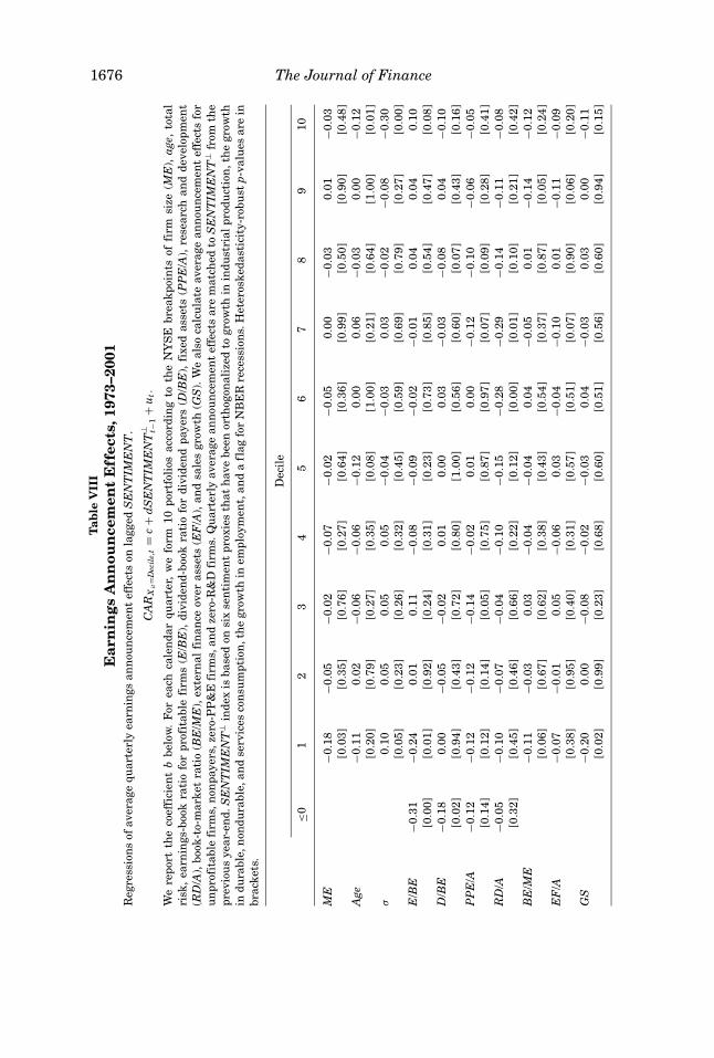
1676 The Journal of FinanceT
able
VII
IE
arn
ings
An
nou
nce
men
tE
ffec
ts,1
973–
2001
Regre
ssio
ns
of
avera
ge
qu
art
erl
yearn
ings
an
nou
nce
men
teff
ect
son
lagged
SE
NT
IME
NT
.
CA
RX
it=D
ecil
e,t=
c+
dS
EN
TIM
EN
T⊥ t−
1+
u t.
We
rep
ort
the
coeff
icie
nt
bbelo
w.
For
each
cale
nd
ar
qu
art
er,
we
form
10
port
foli
os
acc
ord
ing
toth
eN
YS
Ebre
ak
poin
tsof
firm
size
(ME
),ag
e,to
tal
risk
,earn
ings-
book
rati
ofo
rp
rofi
table
firm
s(E
/BE
),d
ivid
en
d-b
ook
rati
ofo
rd
ivid
en
dp
ayers
(D/B
E),
fixed
ass
ets
(PP
E/A
),re
searc
han
dd
evelo
pm
en
t
(RD
/A),
book
-to-m
ark
et
rati
o(B
E/M
E),
exte
rnal
fin
an
ceover
ass
ets
(EF
/A),
an
dsa
les
gro
wth
(GS
).W
eals
oca
lcu
late
avera
ge
an
nou
nce
men
teff
ect
sfo
r
un
pro
fita
ble
firm
s,n
on
payers
,ze
ro-P
P&
Efi
rms,
an
dze
ro-R
&D
firm
s.Q
uart
erl
yavera
ge
an
nou
nce
men
teff
ect
sare
matc
hed
toS
EN
TIM
EN
T⊥
from
the
pre
vio
us
year-
en
d.
SE
NT
IME
NT
⊥in
dex
isbase
don
six
sen
tim
en
tp
roxie
sth
at
have
been
ort
hogon
ali
zed
togro
wth
inin
du
stri
al
pro
du
ctio
n,
the
gro
wth
ind
ura
ble
,n
on
du
rable
,an
dse
rvic
es
con
sum
pti
on
,th
egro
wth
inem
plo
ym
en
t,an
da
flag
for
NB
ER
rece
ssio
ns.
Hete
rosk
ed
ast
icit
y-r
obu
stp-
valu
es
are
in
bra
ckets
.
Deci
le
≤01
23
45
67
89
10
ME
−0.1
8−0
.05
−0.0
2−0
.07
−0.0
2−0
.05
0.0
0−0
.03
0.0
1−0
.03
[0.0
3]
[0.3
5]
[0.7
6]
[0.2
7]
[0.6
4]
[0.3
6]
[0.9
9]
[0.5
0]
[0.9
0]
[0.4
8]
Age
−0.1
10.0
2−0
.06
−0.0
6−0
.12
0.0
00.0
6−0
.03
0.0
0−0
.12
[0.2
0]
[0.7
9]
[0.2
7]
[0.3
5]
[0. 0
8]
[1.0
0]
[0.2
1]
[0.6
4]
[1.0
0]
[0.0
1]
σ0.1
00.0
50.0
50.0
5−0
.04
−0.0
30.0
3−0
.02
−0.0
8−0
.30
[0.0
5]
[0.2
3]
[0.2
6]
[0.3
2]
[0.4
5]
[0.5
9]
[0.6
9]
[0.7
9]
[0.2
7]
[0.0
0]
E/B
E−0
.31
−0.2
40.0
10.1
1−0
.08
−0.0
9−0
.02
−0.0
10.0
40.0
40.1
0
[0.0
0]
[0.0
1]
[0.9
2]
[0.2
4]
[0.3
1]
[0.2
3]
[0.7
3]
[0.8
5]
[0.5
4]
[0.4
7]
[0.0
8]
D/B
E−0
.18
0.0
0−0
.05
−0.0
20.0
10.0
00.0
3−0
.03
−0.0
80.0
4−0
.10
[0.0
2]
[0.9
4]
[0.4
3]
[0.7
2]
[0.8
0]
[1.0
0]
[0.5
6]
[0.6
0]
[0.0
7]
[0.4
3]
[0.1
6]
PP
E/A
−0.1
2−0
.12
−0.1
2−0
. 14
−0.0
20.0
10.0
0−0
.12
−0.1
0−0
.06
−0.0
5
[0.1
4]
[0.1
2]
[0.1
4]
[0.0
5]
[0.7
5]
[0.8
7]
[0.9
7]
[0.0
7]
[0.0
9]
[0.2
8]
[0.4
1]
RD
/A−0
.05
−0.1
0−0
.07
−0.0
4−0
.10
−0.1
5−0
.28
−0.2
9−0
.14
−0.1
1−0
.08
[0.3
2]
[0.4
5]
[0.4
6]
[0.6
6]
[0.2
2]
[0.1
2]
[0.0
0]
[0.0
1]
[0.1
0]
[0.2
1]
[0.4
2]
BE
/ME
−0.1
1−0
.03
0.0
3−0
.04
−0.0
40.0
4−0
.05
0.0
1−0
.14
−0.1
2
[0.0
6]
[0.6
7]
[0.6
2]
[0.3
8]
[0.4
3]
[0.5
4]
[0.3
7]
[0.8
7]
[0.0
5]
[0.2
4]
EF
/A−0
.07
−0.0
10.0
5−0
.06
0.0
3−0
.04
−0.1
00.0
1−0
.11
−0.0
9
[0.3
8]
[0.9
5]
[0.4
0]
[0.3
1]
[0.5
7]
[0.5
1]
[0.0
7]
[0.9
0]
[0.0
6]
[0.2
0]
GS
−0.2
00.0
0−0
.08
−0.0
2−0
.03
0.0
4−0
.03
0.0
30.0
0−0
.11
[0.0
2]
[0.9
9]
[0.2
3]
[0.6
8]
[0.6
0]
[0.5
1]
[0.5
6]
[0.6
0]
[0.9
4]
[0.1
5]

Investor Sentiment and the Cross-Section of Stock Returns 1677
value. The intersection of the two tables’ “strong results” is six cells, and thesigns of the effects are congruent in all cases.
Overall, this suggests that some portion of the conditional characteristicseffects may reflect the correction of errors in earnings expectations. However,as noted above, this test is not powerful and provides only a lower bound on thecontribution of expectational errors.
V. Conclusion
In classical finance theory, investor sentiment does not play any role in thecross-section of stock prices, realized returns, or expected returns. This paperchallenges that view. We use simple theoretical arguments, historical accountsof speculative episodes, and most importantly a set of novel empirical resultsto demonstrate that investor sentiment, broadly defined, has significant cross-sectional effects.
Our main empirical finding is that the cross-section of future stock returnsis conditional on beginning-of-period proxies for sentiment. The patterns arerich but intuitive. When sentiment is estimated to be high, stocks that areattractive to optimists and speculators and at the same time unattractive toarbitrageurs—younger stocks, small stocks, unprofitable stocks, non-dividend-paying stocks, high volatility stocks, extreme growth stocks, and distressedstocks—tend to earn relatively low subsequent returns. Conditional on low sen-timent, however, these cross-sectional patterns attenuate or completely reverse.The most striking finding is that several firm characteristics that display nounconditional predictive power actually hide strong conditional patterns thatbecome visible only after conditioning on sentiment. We consider the classi-cal explanation that the results reflect compensation for systematic risks, butseveral aspects of the results are inconsistent with this explanation.
The results suggest several avenues for future work. In corporate finance,a better understanding of sentiment may shed light on patterns in securityissuance and the supply of firm characteristics that seem to be conditionallyrelevant to share price. In asset pricing, the results suggest that descriptivelyaccurate models of prices and expected returns need to incorporate a prominentrole for investor sentiment.
REFERENCESAghion, Philippe, and Jeremy Stein, 2004, Growth versus margins: The destabilizing consequences
of giving the stock market what it wants, Working paper, Harvard University.
Amihud, Yakov, and Haim Mendelson, 1986, Asset pricing and the bid-ask spread, Journal ofFinancial Economics 17, 223–249.
Asness, Clifford S., Jacques A. Friedman, Robert J. Krail, and John M. Liew, 2000, Style timing:
Value versus growth, Journal of Portfolio Management 26, 50–60.
Baker, Malcolm, and Jeremy Stein, 2004, Market liquidity as a sentiment indicator, Journal ofFinancial Markets 7, 271–299.
Baker, Malcolm, and Jeffrey Wurgler, 2000, The equity share in new issues and aggregate stock
returns, Journal of Finance 55, 2219–2257.
Baker, Malcolm, and Jeffrey Wurgler, 2004, A catering theory of dividends, Journal of Finance 59,
1125–1165.

1678 The Journal of Finance
Banz, Rolf, 1981, The relationship between return and market value of common stocks, Journal ofFinancial Economics 9, 3–18.
Barberis, Nicholas, and Andrei Shleifer, 2003, Style investing, Journal of Financial Economics 68,
161–199.
Barberis, Nicholas, Andrei Shleifer, and Jeffrey Wurgler, 2005, Comovement, Journal of FinancialEconomics 75, 283–318.
Barry, Christopher B., and Stephen J. Brown, 1984, Differential information and the small firm
effect, Journal of Financial Economics 13, 283–294.
Benveniste, Lawrence M., Alexander P. Ljungqvist, William J. Wilhelm, Jr., and Xiaoyun Yu, 2003,
Evidence of information spillovers in the production of investment banking services, Journalof Finance 58, 577–608.
Blume, Marshall, and Robert Stambaugh, 1983, Biases in computed returns: An application to the
size effect, Journal of Financial Economics 12, 387–404.
Brown, Gregory W., and Michael T. Cliff, 2004, Investor sentiment and the near-term stock market,
Journal of Empirical Finance 11, 1–27.
Brown, John Dennis, 1991, 101 Years on Wall Street (Prentice Hall, Englewood Cliffs, NJ).
Brown, Stephen J., William N. Goetzmann, Takato Hiraki, Noriyoshi Shiraishi, and Masahiro
Watanabe, 2003, Investor sentiment in Japanese and U.S. daily mutual fund flows, Working
paper, Yale University.
Brunnermeier, Markus, and Lasse Pedersen, 2005, Predatory trading, Journal of Finance 60, 1825–
1863.
Campbell, John Y., and John H. Cochrane, 2000, Explaining the poor performance of consumption-
based asset pricing models, Journal of Finance 55, 2863–2878.
Chan, Louis K.C., Jason Karceski, and Josef Lakonishok, 2000, New paradigm or same old hype in
equity investing? Financial Analysts Journal 56, 23–36.
Cochrane, John H., 2003, Stocks as money: Convenience yield and the tech-stock bubble, in William
C. Hunter, George G. Kaufman, and Michael Pomerleano, eds.: Asset Price Bubbles (MIT Press,
Cambridge).
D’Avolio, Gene, 2002, The market for borrowing stock, Journal of Financial Economics 66, 271–306.
Daniel, Kent, and Sheridan Titman, 1997, Evidence on the characteristics of cross-sectional vari-
ation in stock returns, Journal of Finance 46, 1739–1764.
De Long, J. Bradford, Andrei Shleifer, Lawrence H. Summers, and Robert Waldmann, 1990, Noise
trader risk in financial markets, Journal of Political Economy 98, 703–738.
Dreman, David, 1979, Contrarian Investment Strategy, Dreman Contrarian Group.
Duffie, Darrell, Nicolae Garleanu, and Lasse H. Pedersen, 2002, Securities lending, shorting, and
pricing, Journal of Financial Economics 66, 307–339.
Elton, Edwin J., Martin J. Gruber, and Jeffrey A. Busse, 1998, Do investors care about sentiment?,
Journal of Business 71, 477–500.
Fama, Eugene F., and Kenneth R. French, 1992, The cross-section of expected stock returns, Journalof Finance 47, 427–465.
Fama, Eugene F., and Kenneth R. French, 1993, Common risk factors in the returns on stocks and
bonds, Journal of Financial Economics 33, 3–56.
Fama, Eugene F., and Kenneth R. French, 2001, Disappearing dividends: Changing firm charac-
teristics or lower propensity to pay? Journal of Financial Economics 60, 3–44.
Geczy, Christopher C., David K. Musto, and Adam V. Reed, 2002, Stocks are special too: An analysis
of the equity lending market, Journal of Financial Economics 66, 241–269.
Gomes, Joao, Leonid Kogan, and Lu Zhang, 2003, Equilibrium cross section of returns, Journal ofPolitical Economy 111, 693–732.
Graham, Benjamin, 1973, The Intelligent Investor, 4th ed. (Harper & Row, Amsterdam).
Greenwood, Robin, and Nathan Sosner, 2003, Trade and the comovement of stock returns: Evidence
from Japan, Working paper, Harvard University.
Gruber, Martin J., 1966, The determinants of common stock prices, Ph.D. dissertation, Columbia
University.
Hausch, Donald, and William Ziemba, 1995, Efficiency of sports and lottery betting markets, In:
Handbooks in Operations Research and Management Science, Volume 9, Elsevier, New York,
NY.

Investor Sentiment and the Cross-Section of Stock Returns 1679
Ibbotson, Roger, and Jeffrey F. Jaffe, 1975, ‘Hot issue’ markets, Journal of Finance 30, 1027–1042.
Ibbotson, Roger, Jody Sindelar, and Jay Ritter, 1994, The market’s problems with the pricing of
initial public offerings, Journal of Applied Corporate Finance 7, 66–74.
Jones, Charles, 2001, A century of stock market liquidity and trading costs, Working paper,
Columbia University.
Jones, Charles, and Owen Lamont, 2002, Short sale constraints and stock returns, Journal ofFinancial Economics 66, 207–239.
Keim, Donald, 1983, Size-related anomalies and stock return seasonality: Further empirical evi-
dence, Journal of Financial Economics 12, 13–32.
Kothari, S. P., and Jay Shanken, 1997, Book-to-market, dividend yield, and expected market re-
turns: A time-series analysis, Journal of Financial Economics 44, 169–203.
Kindleberger, Charles, 2001, Manias, Panics, and Crashes (Wiley, New York).
La Porta, Rafael, Josef Lakonishok, Andrei Shleifer, and Robert W. Vishny, 1997, Good news for
value stocks: Further evidence on market efficiency, Journal of Finance 52, 859–874.
Lakonishok, Josef, and Inmoo Lee, 2001, Are insider trades informative?, Review of FinancialStudies 14, 79–111.
Lakonishok, Josef, Andrei Shleifer, and Robert W. Vishny, 1994, Contrarian investment, extrapo-
lation, and risk, Journal of Finance 49, 1541–1578.
Lamont, Owen A., and Richard H. Thaler, 2003, Can the market add and subtract? Mispricing and
tech stock carve-outs, Journal of Political Economy 111, 227–268.
Lancaster, Kelvin J., 1966, A new approach to consumer theory, Journal of Political Economy 74,
132–157.
Lancaster, Kelvin J., 1971, Consumer Demand: A New Approach (Columbia UP, New York).
Lee, Charles, Andrei Shleifer, and Richard H. Thaler, 1991, Investor sentiment and the closed-end
fund puzzle, Journal of Finance 46, 75–109.
Lettau, Martin, and Sydney Ludvigson, 2001, Resurrecting the (C)CAPM: A cross-sectional test
when risk premia are time-varying, Journal of Political Economy 109, 1238–1287.
Ljungqvist, Alexander, and William Wilhelm, 2003, IPO pricing in the dot-com bubble, Journal ofFinance 58, 723–752.
Loughran, Tim, and Jay Ritter, 1995, The new issues puzzle, Journal of Finance 50, 23–51.
Lowry, Michelle, and G. William Schwert, 2002, IPO market cycles: Bubbles or sequential learning?,
Journal of Finance 57, 1171–1200.
Malkiel, Burton, 1990, A Random Walk Down Wall Street (W.W. Norton, New York).
Malkiel, Burton, 1999, A Random Walk Down Wall Street (W.W. Norton, New York).
Markowitz, Harry, 1959, Portfolio Selection: Efficient Diversification of Investments (Wiley,
New York).
Menzly, Lior, Tano Santos, and Pietro Veronesi, 2004, Understanding predictability, Journal ofPolitical Economy 112, 1–47.
Mitchell, Mark L., Todd Pulvino, and Erik Stafford, 2002, Limited arbitrage and equity markets,
Journal of Finance 57, 551–584.
Neal, Robert, and Simon Wheatley, 1998, Do measures of investor sentiment predict stock returns,
Journal of Financial and Quantitative Analysis 34, 523–547.
Ofek, Eli, and Matthew Richardson, 2002, DotCom mania: The rise and fall of internet stocks,
Journal of Finance 58, 1113–1138.
Peng, Lin, and Wei Xiong, 2004, Limited attention and asset prices, Working paper, Princeton
University.
Reinganum, Marc R., 1983, The anomalous stock market behavior of small firms in January:
Empirical tests for tax-loss selling effects, Journal of Financial Economics 12, 89–104.
Ritter, Jay, 1984, The ‘hot issue’ market of 1980, The Journal of Business 57, 215–240.
Ritter, Jay, 1991, The long-run performance of initial public offerings, Journal of Finance 46, 3–27.
Ritter, Jay, 2003, Some factoids about the 2002 IPO market, Working paper, University of Florida.
Seyhun, H. Nejat, 1998, Investment Intelligence from Insider Trading (MIT Press, Cambridge).
Shiller, Robert J., 1981, Do stock prices move too much to be justified by subsequent changes in
dividends? American Economic Review 71, 421–436.
Shiller, Robert J., 2000, Irrational Exuberance (Princeton UP, Princeton).
Shleifer, Andrei, 2000, Inefficient Markets (Oxford UP, Oxford).

1680 The Journal of Finance
Shleifer, Andrei, and Robert W. Vishny, 1997, The limits of arbitrage, Journal of Finance 52, 35–55.
Siegel, Jeremy, 1998, Stocks for the Long Run (McGraw-Hill, New York).
Smith, E. E., E. J. Shoben, and L. J. Rips, 1974, Structure and process in semantic memory: A
featural model for semantic decisions, Psychological Review 81, 214–241.
Speiss, D. Katherine, and John Affleck-Graves, 1995, Underperformance in long-run stock returns
following seasoned equity offerings, Journal of Financial Economics 38, 243–267.
Spiess, Katherine, and John Affleck-Graves, 1999, The long-run performance of stock returns
following debt offerings, Journal of Financial Economics 54, 45–73.
Stambaugh, Robert F., 1999, Predictive regressions, Journal of Financial Economics 54, 375–421.
Stigler, George J., 1964, Public regulation of the securities markets, Journal of Business 37, 117–
142.
Swaminathan, Bhaskaran, 1996, Time-varying expected small firm returns and closed-end fund
discounts, Review of Financial Studies 9, 845–887.
Wachter, Jessica, 2000, Habit formation and the cross-section of asset returns, Chapter 4 of Ph.D.
dissertation, Harvard University.
Wurgler, Jeffrey, and Katia Zhuravskaya, 2002, Does arbitrage flatten demand curves for stocks?,
Journal of Business 75, 583–608.
Zweig, Martin E., 1973, An investor expectations stock price predictive model using closed-end
fund premiums, Journal of Finance 28, 67–87.