Copyright © 2010 by Daniel Bergstresser and Jeffrey Pontiff

Working papers are in draft form. This working paper is distributed for purposes of comment and discussion only. It may not be reproduced without permission of the copyright holder. Copies of working papers are available from the author.

Investment Taxation and Portfolio Performance Daniel Bergstresser Jeffrey Pontiff

Working Paper

10-084

Investment Taxation and Portfolio Performance1

Daniel Bergstresser Harvard Business School

Soldiers Field Boston, MA 02163

Tel: (617) 495-6169 Fax: (617) 496-5271

Email: dbergstresser@hbs.edu

Jeffrey Pontiff Wallace E. Carroll School of Management

Boston College 140 Commonwealth Avenue

Chestnut Hill, MA 02467-3808 Tel: (617) 552-6786 Fax: (617) 552-0431

Email: pontiff@bc.edu

March 15, 2010

Abstract

Taxes have a first-order impact on portfolio returns. Most research mistakenly assumes

that portfolios command similar tax burdens, or that tax burdens are proportional to dividend

yields. Portfolio strategies differ in the pace of capital gains realization. We use the federal tax

codes from 1926 through 2007 to construct the after-tax returns that individual investors,

corporations, and broker-dealers would have generated on a set of benchmark portfolios. For an

individual at the 99th income percentile, the effective tax rates on SMB and HML, respectively,

are 7 and 15 times greater than the tax rate on the market premium.

1 We thank seminar participants at Arizona State, Boston College, Barclays Global Investors, CRSP Forum, Darden, Harvard/MIT Public Finance seminar, HEC Montreal, NBER Public Economics Program Meeting, Northeastern University, Northwestern, Tilburg, Q-Group, UNC Tax Symposium, University of Amsterdam, University of Arizona, UT Dallas, University of Illinois, Western Finance Association, and William and Mary for helpful comments, as well as David Chapman, Bob Dammon, Joel Dickson, Dhammika Dharmapala, Wayne Ferson, Mike Gallmeyer, Bill Gentry, Clifford Holderness, Edie Hotchkiss, Louis Kaplow, Alan Marcus, Bob McDonald, Jim Poterba, Bill Sihler, Clemens Sialm, Chester Spatt, David Stein, Philip Strahan, and Scott Weisbenner. We thank Angela Chow, Jie He, Sonya Lai, and Karthik Krishnan for research assistance and the Division of Research and Faculty Development at HBS for support.

More than half of corporate equity in the United States is held in taxable accounts.2 Taxes

have a first-order effect on investors’ after-tax wealth accumulation. Investors face two types of

taxes: taxes on dividends and taxes on capital gains. Capital gains are taxed as investors realize

these gains and losses, rather than as the gains accrue. Investors enjoy some flexibility in timing

their capital gains realizations, although portfolio strategies impact this flexibility. Because

deferral reduces the economic burden of taxes, different strategies will impose different tax

burdens.

This paper constructs after-tax returns for benchmark portfolios used by both academics

and practitioners. Differences in tax burdens across these portfolios are driven by two factors.

The first factor is relatively familiar—the differences in dividend payout rates across the

strategies. The second is less familiar—the different patterns of capital gains realization and

deferral that the different portfolio strategies induce. This paper is the first comprehensive

investigation of the latter effect on portfolio performance.

Our main calculations assume realistic “smart” tax-realization strategies, with the

highest-basis shares of given companies sold before lower-basis shares. We show the impact of

taxation using a broad set of equities (all listings on the NYSE) over a long sample (1927–2007).

Instead of assuming static tax rates, our tax rates reflect the actual Federal and New York State

tax codes. Unlike the previous literature, our paper is able to uncover tax effects that are caused

by portfolio styles and by rules that determine index inclusion.

Our study has two main findings. First, we document after-tax portfolio performance.

Second, we show that the tax burden of a portfolio is related not only to the dividend yield, but

also to portfolio style. Portfolio style, by influencing the pattern of capital gains realization,

creates heterogeneity in an investor’s tax burden that is similar to the heterogeneity that stems

from differences in dividend yield.

The CRSP value-weighted index illustrates our results. The effective annual tax burden

on an investor at the 95th percentile of Adjusted Gross Income (AGI) over the period between

1927 and 2007 was 12.28 percent. An investor at the 99.5th percentile of income who was subject

to both federal and New York state taxation had an effective tax rate of 21.48%. Even with the

opportunity to defer the realization of capital gains, taxation has had a first-order impact on

wealth accumulation. 2 See Sialm (2009). This statistic underestimates the historical importance of equity taxation since personal tax-deferred accounts are a recent phenomena.

2

This tax impact can be compared to direct transactions costs, another drag on portfolio

performance that has received considerable attention in the finance literature. A tax-exempt

investor who holds the CRSP value-weighted index and faces a 2 percent round-trip transaction

cost suffers a loss equivalent to 10 basis points per year, whereas an investor paying taxes at

rates corresponding to the 95th percentile of income loses 120 basis points per year.

Although the tax disadvantage induced by high-dividend-yield stocks is well known (see,

for example, Litzenberger and Ramaswamy (1979)), the tax disadvantages associated with

capital gains realization have often been ignored. In general, deferring capital gains realization

lowers tax costs. Different portfolio styles vary in the extent to which they allow investors to

postpone accruing capital gains. Portfolio strategies that involve maintaining equal position

weights, investing in small firms, and investing in value stocks induce early capital gains

realizations. For example, stocks that start out small will often leave the portfolio by becoming

large. Because an investor maintaining a small-firm strategy will constantly sell firms that

become large, this strategy expedites capital gains realization. This creates a high capital gains

tax burden for taxable investors who follow these portfolio strategies.

On the other hand, portfolios where holdings are value weighted, portfolios of large

market capitalization stocks, and portfolios of growth stocks induce a lower capital gains tax

burden. An investor paying the taxes that prevailed at the 99.5th percentile of AGI would have

experienced an effective tax rate of 18.34 percent on a growth stock portfolio and a 26.02 percent

effective tax rate on a value portfolio. For size-based portfolios, the large capitalization firm

portfolio has a 17.81 percent effective tax rate and the small market capitalization portfolio has a

23.73 percent effective tax rate. The momentum portfolio forces high levels of short-term capital

gains realization and has an effective tax rate of 27.30 percent.

In contrast to one-period tax models such as Brennan (1970), which imply that tax

burdens are proportional to dividend yields, we find cases where portfolios with higher dividend

yields have lower tax burdens. Thus, dividend yields are not a sufficient statistic for tax burdens.

The style results carry over to the long-short portfolios that form the Fama-French three-

factor model. For an investor paying the tax rates that prevailed at the 99th percentile of income,

the effective tax rates associated with SMB and HML were, respectively, 7 times and 15 times

the effective tax rate on holding the market risk premium. Although these differences are large,

3

SMB and HML still generate positive after-tax returns, albeit not as extreme as those implied by

the tax-exempt version of the model proposed by Fama and French (1993).

The results documented in this paper are all partial equilibrium results. We take portfolio

strategies, pretax returns, and the structure of tax rates as given, and estimate the after-tax returns

enjoyed by taxpaying investors. We do not argue that all investors pay taxes, or directly present

evidence on the equilibrium impact of taxes on pre-tax returns.3 Our innovation is to consider

portfolios that have been used countless times by practitioners and academics under the tacit

assumption of no taxation, and to offer a precise estimate of these portfolios’ after-tax returns.

Our results have a number of practical implications. First, given the heterogeneity in the

baseline tax burdens for different portfolio strategies, it is appropriate to benchmark portfolio

managers against after-tax benchmarks. Appropriate after-tax benchmarks should consider the

capital gains realizations induced by the trading necessary to maintain a portfolio strategy.

Second, advice to investors about whether equity assets should be held inside or outside

of a tax-deferred account should consider the tax burden induced by different trading strategies.

With respect to tax-deferred retirement accounts, there is some evidence that portfolio managers

consider the tax status of their investors in determining capital gains realization policies. Sialm

and Starks (2009) find that portfolio managers with more defined contribution money appear to

run their funds in a less tax-efficient manner. Our results add to the literature on tax-deferred

retirement investing (see Shoven and Sialm, 2003) by suggesting that some investors should

consider the tax burdens induced by different equity trading strategies in determining whether to

hold particular assets inside of or outside of tax-deferred accounts.

Third, the trade-off theory of capital structure posits that optimal capital structure

balances the costs of financial distress versus the net benefit of corporate tax savings from

interest deductibility minus the costs of taxes incurred by equity investors (see Miller (1977) and

Bradley et al (1984).) Our results suggest that the equity tax cost for the marginal investor will

depend upon which portfolio strategy the marginal investor is following. While the literature has

focused in detail on the statutory tax rate of the marginal investor, our focus considers both

dividend taxation and the effective cost of capital gains taxation after deferral. If all investors

3 Domar and Musgrave (1944) note that it is possible for investors to mitigate capital gains taxation by engaging in risk shifting. This result requires a full offset of capital losses as well as capital gains being assessed on returns above the risk free rate, both of which are at odds with actual tax treatment. Our estimation allows us to consider more realistic offset provisions as well as actual capital gains tax treatment.

4

hold the CRSP value-weighted index in the long-run, and are taxed at the 99th percentile of AGI,

then our results would imply that the effective tax rate on equity is 15.8 percent.

I. Why Does Capital Gains Deferral Matter?

Investors can reduce the burden of capital gains taxes by deferring the realization of their

gains. Deferring capital gains allows investors to earn the extra return on the assets they would

have otherwise liquidated to pay taxes. A simple example, which follows from Chay, Choi, and

Pontiff (2006), illustrates the value of this option to defer the payment of capital gains taxes. Let

r denote the expected return from an asset, and t be the tax rate on realized capital gains.

Consider an investor with $1. If he realizes capital gains in every period, the investor’s expected

terminal wealth after n periods, Wreal, will be

nreal trW )1(1 .

This can be rewritten as

.)1(0

iin

ireal tri

nW

For an investor who defers realization, terminal wealth Wdef of the $1 investment will be

1)1()1( nndef rtrW

or

).1(0

tri

ntW in

idef

The expected value of the difference between these two strategies is

.)1()1(0

iin

irealdef ttri

ntWW

For n>1 and 0<t<1, this difference will be positive, and thus, deferring capital gains realization

will produce higher levels of expected wealth.

The discount rate of this strategy corresponds to the after-tax return that is associated

with realizing every period, r(1-t). Figure 1 shows the impact of the holding period length on the

net present value of capital gains deferral for a range of different values of the underlying

nominal tax rate, and for an assumed pre-tax return of 9.65% (the arithmetic average return of

our S & P index between 1926 and 2007.) The net present values associated with deferral are

substantial. If the capital gains rate is 25%, the decision to hold the stock for eight years, versus

5

realizing a gain every year, is equivalent to 10% of the current investment’s value. This option to

defer accrual of capital gains is at the heart of the analysis in the following sections.

(Insert Figure 1 here)

In many of our simulations, the bulk of the rebalancing occurs annually, since most of

our portfolios are based on characteristics that are determined once per year. Some events,

including delistings, IPOs, share issuance, share repurchases, and dividends, will cause some

month-to-month rebalancing. To the extent that month-to-month rebalancing induces realization

of short-term capital gains, our simulations use the appropriate short-term rate. Long-term and

short-term capital gains tax rates have generally diverged during our sample period. In our

simulations, the required portfolios are determined by the strategies (value-weighted, equal-

weighted, small-firm, large-firm, etc.) We account correctly for the tax basis of individual lots of

shares purchased, and apply the correct tax rate given the holding period observed for each lot of

shares purchased and sold. Most of the analysis in this paper considers the strategy (for long-only

portfolios) of selling highest-basis positions first. This does not create extra trading beyond the

trading required to maintain the simple strategies under consideration. Constantinides (1983,

1984) also considers a tax timing strategy of selling short-term losers and holding long-term

winners. Because this strategy generates trading and transactions costs, we do not use it for our

main simulations, although in Section IV.E we consider the impact of using this strategy.

While we do not consider tax-timing strategies designed to take advantage of the

differences in tax rates applied to long-term and short-term capital gains, our results do capture a

different part of the value transferred to investors through tax deferral. The ability to defer the

payment of taxes, and effectively earn a rate of return on accrued but unrealized capital gains

taxes, is quite large.

II. Constructing Tax Rates, 1927–2007

Our simulation results use two separate approaches to assess the effect of investment

taxation. One approach is to use the actual tax rates that investors were subject to between 1927

and 2007. Because we are interested in constructing portfolio returns enjoyed by investors at

different points in the income distribution, we collect data both on the structure of taxes over the

period, and on the income distribution.

6

The second approach is to assume a static tax environment that is based on the 2000 tax

code. For this approach, we also consider the 2000 tax rules that applied to broker-dealers and

corporations. During the year 2000, corporations were subject to a tax rate of 35% on realized

capital gains and interest. Corporations could exclude 70% of dividends from taxable income,

creating an effective dividend tax rate of 10.5%. Broker-dealers were subject to a 35% nominal

tax rate on capital gains, dividends, and interest received. Unlike individuals and corporations,

capital gains taxes were levied on broker-dealers’ realized and unrealized capital gains.

The different percentiles of the income distribution are taken from Piketty and Saez

(2003).4 Piketty and Saez present data on the level of income (defined as gross income,

excluding capital gains and before taxes) at the 90th, 99th, and 99.5th percentiles of income

distribution back to 1916. Their percentiles are measured in constant dollars; we use the CPI to

deflate these figures to current dollars. Because the Piketty-Saez series ends in 2005, the income

percentiles for the two most recent years are assumed to be equal (in real dollars) to those in

2005. Table I presents data on the income levels at different percentiles near the top of the

income distribution between 1925 and 2005. We use these marginal tax rates to assess the

investment tax cost for various investors at different percentiles of gross income.

(Insert Table I here)

Because stock ownership is concentrated among high-income households, we focus on

the top of the income distribution. Table II, based on data from the 2001 and 2004 Surveys of

Consumer Finances (SCF), demonstrates the concentration in the possession of stocks and

dividends. Our measures of equity holdings include only securities held outside of tax-deferred

accounts; assets held within IRA and 401(k) retirement savings plans would be excluded from

these measures. Indirectly-held equities are held through mutual funds. Table II shows a variety

of thresholds as well as the share of families who report Adjusted Gross Income (AGI) in excess

of each of these thresholds. The table also shows the share of directly-held equity and the share

of directly and indirectly-held equity reported by households above each AGI threshold, as well

as the share of dividends reported by households above each threshold. These results suggest that

in 2000 (the reference year for the 2001 SCF), the median family reported an AGI of between

$25,000 and $50,000. In that same year, the median dollar of direct stockholdings was held by a

4 The income-level data for the different percentiles of income have been periodically updated on Emmanuel Saez’s website, even after the original publication of the paper. See http://elsa.berkeley.edu/~saez/.

7

household with an AGI between $275,000 and $300,000. This is close to the $288,350

breakpoint between the region where income was taxed at a 36% rate and the region where the

marginal federal tax rate on income was 39.6%.

(Insert Table II here)

Including equities held indirectly through mutual funds creates a more egalitarian picture:

the median dollar of direct and indirect equity is held by a household reporting an AGI of

between $200,000 and $225,000. Dividends were even more evenly distributed in 2001: the

median dollar of dividends reported in the 2001 SCF was reported by a household with an AGI

of between $150,000 and $175,000. Dividends were still remarkably concentrated, however: the

household receiving the median dollar of dividends still reported more income than 95% of

households. In addition, the concentration of dividends among high-income investors increased

significantly between 2001 and 2004. This concentration is the reason for our focus on

calculating the after-tax returns for investors in the top decile of the income distribution.

We use a variety of sources to calculate income and capital gains tax rates at each of

these income percentiles in each year. Table III documents some of the changes to relevant

federal tax rates during our sample period. We calculate marginal tax rates separately for

dividends and for capital gains. In addition, we separately measure capital gains tax rates by

holding period, with holding periods of 1–5 months, 6–11 months, 12–17 months, 18–23 months,

2–5 years, 5–10 years, and more than 10 years, with each potentially being subject to a different

tax rate. These distinctions are necessary because of the changing structure of tax rates observed

over time.

(Insert Table III here)

For example, 1997 saw a special medium-term capital gains tax rate, distinct from the

short-term capital gains tax rate and the long-term capital gains tax rate, applied to the sale of

assets held for between 12 and 18 months. The period between 1934 and 1937 also saw a variety

of effective tax rates applied to capital gains on securities, with different rates for stocks held for

less than one year, less than two years, less than five years, less than 10 years, and for more than

10 years.

8

The source for our marginal federal tax rates for the period between 1926 and 1943 is the

1954 IRS Statistics of Income publication.5 These federal marginal tax rates reach a minimum in

1929, when the tax rate on income for investors at the 90th percentile of income was 0.5 percent.

The period of the maximum federal marginal tax rate varies across the income distribution, in a

pattern reflecting changes in the progressivity of the federal tax code at very high income levels.

The maximum overall marginal tax rate came in 1944, when the total federal tax rate on an

investor at the 99.99th percentile of income was 92 percent. In that year, however, the marginal

tax rate at the 99th percentile of income was 41 percent. The maximum tax rate at the 99th

percentile was 55 percent, reached in 1978. The maximum tax rate at the 99.5th percentile was 59

percent, reached in 1979 and 1980. In each of those years the marginal tax rate at the 99.99th

percentile was 70 percent.

The federal marginal tax rates between 1944 and 1987 come from Pechman’s (1987)

reference on American income taxes. Marginal federal tax rates in the period after 1987 are

derived from the IRS Instructions for Form 1040 for each of the years during that period.

Some of our calculations consider New York state tax. New York has consistently been

among the most populous states, and its residents are relatively wealthy. Among the other very

large states, California has higher marginal tax rates income and Texas and Florida have no state

income tax. Given the consistently large weight of New York in financial markets, using that

state’s tax rates to illustrate the impact of state-level taxation is appropriate.

New York state taxes were particularly high during the 1960s and 1970s, with tax rates

on dividends topping out at 15 percent from 1973 to 1978. Tax rates on capital gains during this

period were lower, with rates on long-term gains peaking at 9 percent during the same period.

For our assumed 99.5th percentile investor, tax rates have more recently fluctuated between 6.8

and 7.9 percent. Our simulations assume that New York state taxes are deductible from federal

income taxes.

Our main calculations assume that all capital losses in the portfolio can be used in the

current year. This can be a counterfactual assumption; capital losses can be used to offset capital

gains in the current year, and currently $3,000 worth of capital losses can be used to offset

ordinary income. In reality, capital losses that are realized, but that cannot be used to offset

5 Special thanks to Clemens Sialm for sending his copies of these data publications.

9

capital gains or ordinary income (because they exceed the limit of total capital gains, plus $3,000

in ordinary income), may be carried forward. Our assumption that capital losses can be used to

offset capital gains in the current year is appropriate for an investor who also has a separate large

portfolio on which capital gains are continuously being realized. In order to assess the sensitivity

of our results to the full-offset assumption, we also consider results in Section IV.E that only

allow net losses to be carried over to future periods.

III. Return Data

Our data on stock prices, splits, distributions, mergers, and delistings come from the

CRSP database. For distributions and delistings, we apply the appropriate tax rates for the given

hypothetical investor.

A. Constructing Portfolios

Portfolios are constructed on the basis of market equity, book-to-market ratio, and firms’

dividend policies. Book equity data for the period since 1962 come from Compustat, and

measures of book equity are constructed according to the procedures detailed in Davis, Fama,

and French (2000). For the period before Compustat coverage, book equity data come from the

U.S. Historical Book Equity data that are available on Ken French’s website.6

For the portfolios based on firm size, book-to-market, and momentum, decile cutoffs are

also taken from Ken French's data library. The portfolios are constructed based on the sample of

firms listed on the New York Stock Exchange. We focus on the value-weighted portfolios of

firms in the top and bottom quintiles. Firms are sorted into size quintiles based on their market

equity capitalization at the end of the most recently completed month of June. For the months of

July through December, firms are sorted into book-to-market quintiles based on their ratio of

book equity to market equity as of the end of the previous year. For the months of January

through June, firms are sorted into BE/ME breakpoints based on their level as of the next-to-last

December. Firms are placed in momentum quintiles based on stock performance between 12

months and two months earlier. For the market capitalization, book-to-market, and momentum

extreme quintile portfolios, each stock is weighted by its market capitalization; thus, some

6 http://mba.tuck.dartmouth.edu/pages/faculty/ken.french/data_library.html

10

rebalancing is needed for each month to reflect events such as distributions, share issuance, share

repurchases, and delistings. For the market capitalization and book-to-value portfolios, heavy

trading from the change in cut-off values is induced in the month of July. For the momentum

portfolios trading is more evenly dispersed across the calendar year.

Dividend-based portfolios are constructed based on firms' dividend policies in the most

recently completed years. Firms are allocated first to portfolios of dividend payers versus non-

dividend payers. Among dividend-paying firms, firms are broken down into firms whose

dividend policies in the previous year place them among the top half of dividend-paying firms

(in terms of the dividend payout ratio to lagged share price), and those whose dividend policies

place them among the bottom half of dividend-paying firms. The policy of assigning firms to

dividend-based portfolios based only on the information in subsequent years makes these

portfolios somewhat more trading-intensive than they would be if we constructed portfolios

based on longer patterns of dividend events. Again, each firm’s weight in each dividend portfolio

is proportional to its market capitalization.

Additional simulations are based on constructing a value-weighted portfolio of the NYSE

stocks (VWRET), and an equally-weighted portfolio of NYSE stocks. The VWRET portfolio

requires limited trading to maintain, and the average turnover for that portfolio is below 4

percent per year. The EWRET portfolio requires much more trading, with monthly rebalancing

to maintain equal weights on the stocks in the portfolio as their market prices fluctuates. Finally,

we run simulations with the stocks included in the S & P index. Because the S & P 500 was only

created in 1957, for the period before 1957 we use the S & P 90, the benchmark that was

superseded by the larger index. We refer to the entire series as the “S & P.”

B. Constructing Portfolio Returns

All portfolios include only stocks listed on the NYSE. This restriction eliminates drastic

portfolio changes when NASDAQ data enter the CRSP dataset. The analysis starts in June of

1927, with a portfolio of $100 in long positions and $100 in short positions. Focusing on the long

side, the $100 is allocated across the stocks, depending on the strategy chosen. For instance, if

the strategy chosen is a value-weighted portfolio of the smallest half of the shares in the market,

then the weights within this portfolio are set accordingly. All long portfolios are totally self-

financing; thus, all distributions are reinvested in the portfolio and all taxes are paid through a

11

partial liquidation of positions. We also consider strategies that involve both a long and a short

portfolio. For these strategies, the value of the short portfolio is re-adjusted every month to

equate to the long portfolio, causing the short portfolio to consume or generate cashflow.

The long portfolio’s value in July 1927 depends on the pattern of distributions, delistings,

and changes in price over the preceding month. The program that calculates the portfolio return

first accounts for all of these distributions and delistings, paying the appropriate taxes and

recording the amount of cash on hand after these distributions are made. Then, the appropriate

portfolio weights for the next month are chosen. These portfolio weights may be different from

the preceding month, if stocks have moved in to or out of the portfolio under consideration. For

instance, if we are analyzing the return to the small-firm strategy, and a firm moves beyond the

relevant market equity size breakpoint, then its weight starting in the month that it moves out of

the relevant group will be zero.

The long portfolio is reallocated according to the new desired portfolio weights.

Reallocation involves the realization of some capital gains or losses, since some stocks are being

purchased and some sold. The realization of capital gains, for a taxable investor, means that the

reallocation to the new desired portfolio weights imposes a new round of taxes in the simulation.

This round of taxes is in addition to the taxes that were involuntary, based on the distribution of

dividends and on capital gains realized through the removal of companies from the portfolio. In

our simulation, the taxes paid on these gains change the size of the portfolio in that month,

leading to a new round of capital gains realizations. These capital gains realizations, in turn,

create a new set of taxes. Our approach is to iterate three times down this path. Three iterations

bring us very close to the fixed point where the capital gains taxes that must be paid are precisely

payable given the cash taken from the portfolio from the net sale of stock.

The simulation routine keeps track of the basis of each of the shares in the portfolio,

adjusting the per-share basis as necessary for distributions and for corporate events such as stock

splits. To calculate the long-portfolio returns, the simulation routine preferentially liquidates the

high-basis shares, in order to defer the realization of capital gains. Section IV.E considers the

robustness of our findings to this assumption.

The simulation routine is also capable of considering long-short portfolios. Examples are

zero-investment portfolios such as the Fama-French SMB and HML portfolios. In each period

the size of the short portfolio is adjusted to equal the size of the long portfolio, through the sale

12

or purchase of the correct number of shares (keeping the appropriate portfolio weights). This

reallocation requires either an infusion or a withdrawal of cash. Adding cash to the short

portfolio is necessary when the value of the short portfolio has fallen relative to the value of the

long portfolio; we therefore consider the net cash added to the short portfolio, in each period, as

a measure of the performance of the long portfolio relative to the short.

The other difference in the short portfolio is the assumption we make about the tax basis

of the shares moved in to and out of the portfolio. We make the assumption that, as shares move

out of the portfolio, the low-basis shares are chosen. In contrast, the long-portfolio returns are

constructed assuming that the high-basis shares are liquidated first.

We assume that the capital gains rate that applies to the short portfolio is the same as the

rate that would apply to the position’s holding period. This treatment departs from stand-alone

taxation of short sales, for which all short sales are taxed as short-term gains. This treatment is

correct to the extent that the investor also holds a large long portfolio that includes long positions

in the shorted stocks. Thus, our tax rate assumption assumes that the investor holds the market

and deviates slightly with long-short portfolios, such that the net exposure remains long.

C. Portfolio Values, Liquidation Values, and Continuation Values

Calculating an after-tax return to a portfolio strategy requires an assumption about the

after-tax value of the capital gains that accrue but remain unrealized in the portfolio. Two polar

approaches are available. One approach is to construct a return based on the value of the stocks

held in the portfolio. This approach assumes a zero effective rate of taxation on the accrued but

undistributed capital gains in the portfolio. This assumption would be appropriate for an investor

who planned to pass the assets to heirs through an estate and thereby enjoy the step-up in capital

gains that occurs at death. An opposite approach would be to calculate in each month the value

of the cash that the investor would have after liquidating the portfolio and paying the appropriate

capital gains taxes on the accrued capital gains. This assumption is appropriate for an investor

with a very short horizon.

Approaches between these two polar cases calculate a value of the portfolio that assumes

that the effective tax rate on accrued but unrealized capital gains is lower than statutory rates but

higher than zero, due to the investor’s option to defer the realization of gains. Our results in the

13

sections that follow are based on a calculation of the “effective” value of the portfolio, which is

based on an assumption between these polar cases:

Effective value = Liquidation value + λ x (Nominal value – Liquidation value) (1)

“Nominal value” is still influenced by taxes since the portfolio is self-financed and capital gains

are paid when the portfolio is rebalanced. For each of these measures of the value (liquidation

value, nominal value, and effective value), a log long-return measure is constructed each month

as the change in the log of this measure. Our expression for “effective value” was originally

developed in Stein (1998). Stein stresses that λ is a function of beliefs about expected returns as

well as investor characteristics such as tax rates and expected investment horizons. Our

calculation is simplified by always setting λ=0.193. 0.193 is the value of capital gains deferral as

a fraction of capital gains taxes paid upon immediate liquidation. This estimate is constructed

using an assumed nominal capital gains tax rate of 28% and the Chay, Choi, and Pontiff (2006)

finding that one dollar of realized capital gains equates to 93¢ of unrealized gains7.

We have checked the robustness of our results to this assumption and have found

relatively minor sensitivity of our results to λ. For example, varying λ from 0 to 1 produces

estimates of annualized returns on long portfolios that vary by, at most, 15 basis points. For our

estimation, the choice of λ tends to be minor since we calculated continuously compounded

returns over a very long time period. Continuous compounding is largely unaffected by prices

over the intermediate periods.8 Thus, the return is affected primarily by the initial price, the final

price, and the stream of dividends. The impact of the final price is small relative to the high

present value that is associated with an 80-year stream of dividends.

We describe the returns to short portfolios as well as long-short portfolios. Unlike the

long portfolios, which are entirely self-financed, the short portfolios are subject to monthly cash

inflows and outflows, which reset the pre-tax short portfolio value to that of the long portfolio.

7 The drop-off-ratio of realized capital gains to unrealized price appreciation in Chay, Choi, and Pontiff (2006) is 0.93. For the marginal investor, this equates to

imp

cg

T

T

1

1 . Tcg is the nominal capital gains tax rate and Timp is the

implied capital gains tax rate, which considers the value of deferral. If the nominal rate is 28% a drop-off ratio of 0.93 implies that the implied capital gains tax rate is 22.58%, which is 19.36% lower than the nominal rate. 8 If Pt denotes the price of non-dividend-paying stock in period t, then the log return over n periods is ln(Pt+n/Pt), regardless of the value of prices between t and t+n.

14

The short-portfolio return is calculated as the difference of the log of the sum of the current

period’s cashflow to the portfolio and the current period’s effective value, minus the log of the

last period’s effective value.

For the long-short portfolio return, we first add the effective value of the long portfolio

with the cashflow generated from the short, and subtract from this the change in the short

portfolio’s effective value. We divide this measure by the last period’s effective value on the

long portfolio. We use the log of this ratio as our long-short return.

In addition to calculating measures of portfolio value and measures of returns, we can

also calculate a measure of the “capital gains overhang” for each portfolio. This overhang is the

normalized difference between the nominal value and the liquidation value:

Overhang = (Nominal value – Liquidation value)/Nominal value (2)

This overhang will increase as the share of accrued but unrealized capital gains in the portfolio

rises, and as the statutory capital gains tax rates rise. Over time, a strategy that successfully

defers realizing capital gains (thereby decreasing the present value of the tax burden) will create

a portfolio with a substantial overhang of unrealized capital gains.

Since we use continuously compounded (natural log) returns, a comparison between

returns for various strategies reveals the actual performance difference between the strategies.

Along these lines, for each tax level associated with each strategy, we compute an effective tax

rate, as well as an effective capital gains tax rate and an effective dividend tax rate. The effective

tax rate is computed by taking the difference between the log return of a tax-exempt investor and

the log return of a taxed investor, and then dividing that difference by the log return of the tax-

exempt investor. Thus, the effective tax rate measures the proportion of the tax exempt investor’s

performance that would have been consumed by taxes. The effective capital gains tax rate and

the effective dividend tax rate are calculated in a similar manner. For the effective capital gains

(dividend) tax rate, we calculate the log return of a taxable investor, under the assumption that

the investor is rebated all dividend (capital gains) taxes each period. We calculate the difference

between this return measure and the tax-exempt return, and divide by the tax-exempt return.

Since the performance differences between the tax-exempt and taxable investor are caused

entirely by either dividend or capital gains taxes, this measure calculates the actual impact of

15

these taxes on performance. In addition, since we measure the percentage difference of log

returns, the effective capital gains tax rate and the effective dividend tax rate do not add up to the

total relative tax cost. The small discrepancy is caused by a Fisher effect.

The interpretation of the effective capital gains and dividend tax rates is different from

the interpretation of the nominal capital gains and dividend tax rates. For example, the nominal

dividend tax rate tells us the incremental cost of receiving an extra dollar in dividend income,

whereas the effective dividend tax rate describes how dividend taxes diminish after-tax returns.

If a portfolio never pays a dividend, the effective dividend tax rate would be zero, despite the

fact that the nominal dividend tax rate is positive.

IV. Results

This section presents three different types of results. The first subsection (subsection

IV.A, and Table IV) investigates the impact of selecting the basis of shares to sell on the returns

to different portfolio strategies. These results illustrate both the impact of taxation on the returns

to the different strategies, and the impact of the assumption that investors optimize by selecting

high-basis shares for sale.

The next subsections (subsections IV.B–IV.F) describe the impact of taxation on the

returns to different benchmark portfolios. The tables in these subsections (Tables V–IX) have

two panels. The A panels in these tables report the actual after-tax returns an investor would

have received, assuming the investor paid taxes according to the federal tax code at the time. The

A panels provide a historical record of the actual after-tax performance of the investment

strategy. The effective tax rates that we calculate in the A panels are influenced by intertemporal

changes in the tax code. For example, a strategy that realizes capital gains in a time period where

nominal capital gains rates were low will have a lower historical effective tax rate than a strategy

that realizes gains after an increase in nominal rates. The B panels examine the after-tax returns

that investors would have earned under the counterfactual assumption that tax rates were fixed

throughout the period at the rates prevailing in 2000. To the extent that corporate managers

consider taxes in making decisions about dividends and share issuance, the results that use the

2000 rates will overstate effective tax rates.

Figure 2 provides an overview of our results. It compares pre-tax and after-tax returns for

an investor at the 99.5th percentile of income who was subject to both federal and New York

16

State taxation. The tax rates used in the simulations are the historically accurate rates. The figure

also compares returns for a hypothetical corporate investor who paid tax based on the tax rates

that prevailed in the year 2000. The (negative) slope of the line connecting the pre- and after-tax

returns for each strategy is proportional to the size of the wedge between pre-tax and after-tax

returns. For the pairings with more negative slopes, the size of this tax wedge has been greater.

The figure illustrates how different the effective taxation on different portfolios has been, even

for the same investor. There are some cases where a ranking of portfolios based on average pre-

tax returns does not map to the ranking based on after-tax returns. For example, for the

individual investor, the pre-tax return on the high dividend portfolio is higher than that of

EWRET, but the after-tax return is lower. For the corporate investor, although the pre-tax return

to the momentum portfolio is higher than the pre-tax return of the value portfolio, after-tax the

momentum portfolio has a slightly lower return.

(Insert Figure 2 here)

A. Fundamental Long Strategies

Table IV reports the after-tax returns to broad portfolios and portfolios that are

determined by dividend yields. The table also presents the after-tax returns to a strategy of

holding three-month treasury bills, our reference “risk-free” asset. Since dividend yields and

turnover influence strategy tax burdens, we present (in parentheses next to the name of each

portfolio) the annual dividend yield and annual turnover associated with the tax-exempt strategy

portfolio. For each portfolio, Table IV presents five different results. The first row of results

shows the average of the natural log of after-tax returns. The second row shows the average

percentage of overhang. The third and fourth rows detail the percentage of decrease in the return

that is attributable to, respectively, capital gains and dividends. The fifth row shows the total

effective tax rate.

(Insert Table IV here)

The portfolios described in Table IV span a range of dividend yields and turnover. The

no-dividend portfolio has a dividend yield of 0.56% annualized. This reflects companies that

paid no dividends in the previous year but initiated dividends in the current year. The highest-

dividend-yield portfolio is the high-dividend portfolio with an annualized yield of 5.46%. The

lowest-turnover portfolio is the CRSP value-weighted portfolio; this portfolio has an annualized

17

turnover of 3.98%. The highest-turnover portfolio is the CRSP equal-weighted portfolio, which

has an annualized turnover of 44.76%.

Panel A in Table IV shows that, historically, the Treasury bill is most tax disadvantaged.

Out of the equity portfolios, the high-dividend-yield portfolio is the most tax disadvantaged,

followed by the equal-weighted portfolio. The equal-weighted portfolio tends to have an

effective tax rate that is about 2% higher than those of the value-weighted and S & P portfolios,

despite the fact the equal-weighted portfolio has a dividend yield lower than both portfolios. A

similar (although less pronounced) result occurs in comparing the low-dividend portfolio with

both the S & P portfolio and the value-weighted portfolio. Although the low-dividend portfolio

has a slightly higher dividend yield than the other two portfolios, it enjoys a lower effective tax

rate for all levels of investor income. These findings contradict the common assumption that

dividend yields proxy for tax burden.

Figure 3 shows the growth over time in the portfolio values for four of the equal-

weighted portfolios. For each portfolio, the value in each period is calculated gross of an

overhang of capital gains taxes that would need to be paid upon portfolio liquidation. Figure 4

shows growth over time for three of the value-weighted market portfolios. By June of 2007, the

untaxed equal-weighted portfolio that started with $100 in 1927 is worth $1,843,000. The

untaxed value-weighted market portfolio was worth $252,000 by June of 2007.

(Insert Figure 3 here)

(Insert Figure 4 here)

Figure 5 illustrates the relative tax burdens of the equal-weighted and value-weighted

portfolios. For an investor paying tax rates prevailing at the 95th percentile of income, the equal-

weighted portfolio was worth $497,000, or 27 percent of the value of the untaxed portfolio. For

the 95th percentile investor in the value-weighted portfolio, the final portfolio value was 41

percent of the value of the untaxed value-weighted portfolio. At the higher tax rates prevailing at

the 99.5th percentile of income, the taxable investor in the equal-weighted portfolio ends with a

portfolio that is 14 percent the size of the untaxed equal-weighted portfolio; a taxable investor in

the value-weighted portfolio ends with a portfolio that is 27 percent the size of the untaxed

value-weighted portfolio. For an investor in the 99.5 AGI percentile who is also subject to New

York state tax, the respective relative value of the taxed equal- and value-weighted portfolios is

18

11 percent and 22 percent. Thus, over this 80 year period, the New York state taxation reduced

by half the total wealth accumulation of a taxable investor.

(Insert Figure 5 here)

For all portfolios other than the no-dividend portfolio, dividend taxation represents a

larger share of the total tax cost than capital gains taxes. The impact of capital gains taxation

varies much more widely across portfolios, however. In the case of the equally-weighted

portfolio, the impact of capital gains taxes is almost as large as the impact of dividend taxes.

The three dividend portfolios demonstrate the interaction between capital gains and

dividend tax burdens. Many studies have used dividend yield as a proxy for the tax cost of a

portfolio.9 Consistent with these studies, the no-dividend portfolio has the lowest tax burden of

the three dividend-based portfolios, followed by the low-dividend portfolio and then the high-

dividend portfolio. A dividend proxy for tax cost understates the tax burden in the case of the no-

dividend portfolio, since this portfolio has the highest capital gains cost. The high capital gains

cost comes because non-dividend payers that initiate dividend payments are likely to have price

appreciation in the initiation year. Since dividend initiation forces them out of the no-dividend

portfolio, the rebalancing induced by the maintenance of the no-dividend portfolio strategy leads

to higher capital gains realizations.

The dividend portfolios also display an interesting turnover pattern. The low-dividend

portfolio has a much lower effective capital gains tax rate than the no-dividend and high-

dividend portfolios. The low-dividend portfolio has effective capital gains tax rates that range

from one-tenth to one-half the rates of the other two portfolios. This finding is consistent with

the fact that the low-dividend portfolio has an annual turnover of 6.81 percent, while the other

portfolios have turnover levels of over 30 percent. We expect that these results are related to not

only turnover from one dividend portfolio to another, but also to turnover related to firm exit

from the NYSE universe. The overall message is that although creating dividend-sorted

portfolios may group stocks based on dividend tax burdens, capital gains burdens are affected by

the trading rules needed to maintain the dividend-based portfolios.

Although total effective tax increases with income level for both the S & P and the value-

weighted index, the highest income levels sometimes show a decrease in the portion of the tax

9 See, for instance, Litzenberger and Ramaswamy (1979).

19

rate attributable to capital gains taxes. This seemingly odd result is noticeable for many

portfolios that we consider. During our sample period, capital gains tax rates reached their

maximum levels at lower-income thresholds than dividend tax rates. Because of this, investors

with the very highest incomes re-invested a lower proportion of their portfolio dividends than

investors with somewhat lower incomes. In our simulations, lower dividend reinvestment

decreases the total value of future capital gains relative to the tax-exempt portfolio, creating a

crowding-out effect that reduces the measured effective capital gains tax rate.

These results indicate that the effective tax rate on accruing but unrealized capital gains

will depend on the investment strategy of the portfolio, even when the portfolio is being

managed in a tax-efficient way. Strategies such as the value-weighted strategy offer more ability

to defer capital gains, leading to a lower effective tax rate on accruing capital gains. Contrary to

this result, previous empirical work has often assumed a fixed effective tax rate on accruing

capital gains. For example, Bergstresser and Poterba (2002) apply a blanket effective tax rate of

10 percent to accruing capital gains in their calculation of after-tax mutual fund performance

measures.

While Panel A of Table IV calculates returns based on actual historical tax rates, Panel B

presents the returns that investors would have earned had the rates prevailing in 2000 applied

throughout the period. Both panels use the same realization rule—highest-basis positions are

sold first. The historical results in Panel A may result in unrealized gains being delayed until

realization in a tax regime that is either higher or lower. By holding tax rates constant through

time, Panel B’s results are not subject to contamination by idiosyncrasies in the historical pattern

of tax rates.

Using the individual tax rates from 2000 produces lower effective tax rates across the

board. The risk-free security continues to have the highest tax burden. The value-weighted index

is now more tax burdensome than the equal-weighted index, although the share attributed to

capital gains is still higher for the equal-weighted portfolio. Overall, the Panel B results are

similar to those for Panel A. One clear difference is that the effective tax rates using the 2000 tax

code produce tax effects that are less progressive than those under the historical code.

Panel B also considers how the 2000 tax code would have affected the portfolios held by

corporations and securities dealers. The advantage of lower dividend taxation for corporations is

apparent. With the exception of the no-dividend portfolio, the effective tax rate borne by

20

corporations holding the equity portfolios is substantially lower than the rate faced by

individuals. For this portfolio, the effective tax rate that corporations face is over 14 percent,

whereas individuals at all income levels face effective tax rates that are lower than 9 percent.

Broker-dealers bear the highest effective tax rates for equity portfolios. Their effective tax rates

on all of the equity portfolios tightly range from 29 percent to 32 percent, with the exception of

the no-dividend portfolio, which has a 22 percent effective rate.

B. Style Portfolios

Table V reports the after-tax return to value-weighted portfolios that use five different

investment styles, based on market capitalization, book-to-market, and return momentum. Based

on the historical tax rates presented in Panel A, the style portfolios are (roughly) sorted from

lowest to highest effective tax rates. The various portfolios exhibit substantial differences in

effective tax rates. For many levels of AGI, the highest-tax portfolio (momentum) has an

effective tax rate that is one and a half times that of the lowest-tax portfolio (large market

capitalization). The fact that winner stocks are sold in the value and small-firm portfolios is

associated with higher effective tax rates than the large and growth portfolios. The effective tax

rates on value and small portfolios are about 4–8 percentage points higher than large and growth.

Value portfolios are particularly tax disadvantaged since they are exposed to suboptimal capital

gains realization and high-dividend yields.

(Insert Table V here)

Similar to the findings in Table IV, dividend yields are an imperfect proxy for effective

tax rates. The small-firm portfolio has the lowest-dividend yield, despite the fact that its effective

tax rate is higher than the portfolios’ growth stocks and large stocks.

The momentum portfolio has the highest effective tax rates. This may be attributable to

the fact that they involve high turnover and that positions are often sold with short-term capital

gains, which carry a higher nominal rate than long-term gains.

Portfolios with higher average returns have higher effective tax rates. The effective tax

rates have the effect of decreasing after-tax heterogeneity—differences across portfolios in after-

tax returns tend to be less extreme than differences across portfolios in pre-tax returns. Thus,

studies that find cross-sectional return predictability, overstate cross-sectional return differences

for taxable investors. Despite this, taxation does not negate the differences in return levels: after

21

tax, the value portfolio still outperforms the growth portfolio and the small-firm portfolio still

outperforms the large-stock portfolio.

Panel A also reveals the progressivity that has prevailed in tax rates on high-income

taxpayers. Effective tax rates on federal-only taxpayers at the 99.5th percentile of income have

effective tax rates that are about 50 percent greater than those at the 95th percentile. Panel B

documents the differences assuming that the 2000 tax code held throughout the 1927–2007

period. In addition to individual investors, the panel also considers corporate investors and

broker-dealers. Although the general pattern remains, with small and value having the largest tax

burdens, the growth portfolio edges out the large-firm portfolio as having the lightest tax burden.

The 2000 tax code produces less extreme effective tax rates than using the actual tax rates over

1927–2007. For example, the effective tax rate for the 99.5th percentile AGI investor is only 10

to 20 percent greater than that of the 95th percentile investor. Similarly, using the 2000 tax code

mutes somewhat the differences in effective tax burdens between the portfolios with high and

low effective tax rates.

The effective tax rates associated with corporate investors exhibit more heterogeneity.

Like Panel A, they enjoy a low effective tax rate for the large capitalization portfolio. Their tax

rate on the momentum portfolio is more than three times the tax rate on the large firm portfolio.

Broker-dealers face the highest effective tax rates of all investors considered in Panel B. Because

broker-dealers face taxation on all realized and unrealized gains, their effective rates across

portfolios are similar in magnitude.

C. Long-Short Portfolios

Fama and French (1993) propose a multi-factor model of stock returns based on three

factors: the return of the value-weighted market index minus the risk-free rate (VWRET-RF), the

return of small minus big market capitalization stocks (SMB), and the return of high minus low

(HML) market-to-book stocks. The typical formulation of the Capital Asset Pricing Model

(CAPM) relies on a single market factor, VWRET-RF. The ability of the Fama-French three-

factor model to provide an improvement in explaining cross-sectional return variation depends

on the factors HML and SMB having non-zero return expectations.

We construct the after-tax performance for all three of the Fama-French factors. We

assume that purchases and sales on the short side of the portfolios generate capital gains taxes at

22

the rate that corresponds to the position’s holding period. This treatment is symmetrical to the

treatment of capital gains on the long side of the portfolio, although it is counter to IRS rules that

use the short-term capital gains rate for all short sales, regardless of the actual holding period.

Our decision to treat short sales is consistent with investors holding the value-weighted market

portfolio and picking exposure to SMB and HML, such that they are not net short. Thus, the

short side represents a lower exposure to positions that are already in the value-weighted

portfolio, and our estimation will tell us about the impact of making a tilt permutation from the

market portfolio toward value and/or small market capitalization. Our findings will be of

relevance to long-only investors.

The construction of the factors follows Fama and French (1993) identically. Table VI

reports the after-tax performance of these portfolio strategies. The broad results are consistent

with the long-only results in Tables IV and V. Panel A of Table VI presents results that use the

time-appropriate tax rates. The market premium portfolio commands low effective tax rates,

consistent with the benefit of going long the low-tax market portfolio while shorting the high-tax

risk-free rate. The most heavily taxed investor (at the 99.5th percentile of AGI and subject to both

federal and New York state tax) faces an effective tax rate of only 4.15 percent on this portfolio.

Both the SMB and HML portfolios face a higher effective tax rate than does the market premium

(VWRET-RF) portfolio. For an investor taxed at the 99th percentile of income, the effective tax

rate of the SMB portfolio is nearly 7 times that of the market premium (9.92/1.46). For this same

investor, the tax cost of HML is over 15 times that of the market premium. The differences

between the relative tax cost of the SMB portfolio and the HML portfolio have been less extreme

for the most highly-taxed investors.

(Insert Table VI here)

Despite the drastic effective tax rates that style factors command, SMB and HML still

have positive after-tax returns. Investment taxation reduces but does not negate the premia

associated with these factors.

Panel B of Table VI presents the returns that investors, corporations, and broker-dealers

would have earned had the 2000 income tax rates prevailed over the entire period. Again,

individual investors focusing on the SMB and HML portfolio strategies face much larger

effective tax rates than an investor limited to investing in the market risk premium, although the

magnitudes are less extreme than in Panel A. For all levels of AGI, the effective tax rates on

23

SMB and HML are about three times the rate of the market risk premium. Corporate investors

face higher effective rates on all three factors than individual investors, although the pattern is

very similar—the effective rates on SMB and HML are about three times the rate of the market

risk premium. Broker-dealers depart from these groups: although their effective tax rates on

SMB and HML are similar in magnitude to corporations, their effective tax rate on the market

risk premium is nearly identical to the other factors. This is because they cannot defer the

realization of accruing gains, even on portfolios that would offer the opportunity to do so. Thus,

for broker-dealers the relative return tradeoff between the three factors is almost identical to that

of a tax-exempt investor.

D. The Impact of Loss Treatment

The current U.S. tax code allows investors to deduct up to $3,000 per year in net realized

losses from their ordinary income. Any net loss in excess of $3,000 is carried forward to the next

year, where it may be used to offset realized capital gains. Net losses may be carried forward

indefinitely, until the death of the investor, at which point they expire with no value. Our

previous results assumed that realized losses immediately generate a positive cashflow equal to

the holding-period appropriate capital gains tax rate times the loss. This treatment generates

after-tax returns that correspond to incremental cashflows to an investor who holds other

securities that generate unlimited capital gains, for which losses on the examined portfolio may

be deducted.

In this section we consider a second approach for the use of losses. We carry forward

losses until they can be used to offset gains in the portfolio. This generates results that describe

the after-tax investment performance of an investor who holds a portfolio in isolation. In this

case, all realized losses are valuable only to the extent that they can be carried forward and used

to offset future realized gains. Each month long- and short-term realized gains are used to offset

long- and short-term realized losses. If losses are greater than gains, the loss is carried over to the

next month. Similar to the U.S. tax code (although on a monthly frequency), we preserve short-

term and long-term losses separately, and use short-term losses to offset short-term gains; and

long-term losses to offset long-term gains.

Carrying forward losses generally increases effective investment tax rates, relative to

using the losses immediately. Carrying forward losses is particularly disadvantageous for

24

portfolios that create short-term capital gains realization, since it increases the chance that a

short-term loss is used to offset a long-term gain, which is less valuable than offsetting a short-

term gain.

Table VII compares the historic effective investment tax rates for individuals at the 99th

percentile of AGI as well as the effective tax rates for individuals and corporations, assuming

that the 2000 tax code was in effect throughout our sample. For brevity, we focus on these three

tax rate assumptions. The pattern of results, in terms of the comparison of carrying forward

losses versus using them immediately, is similar for other tax rate assumptions.

(Insert Table VII here)

For all three of these specifications, the momentum portfolio generates the most dramatic

results. Using losses immediately dramatically reduces the effective tax rates on the momentum-

based portfolios. We attribute this result to the high frequency at which short-term capital losses

accrue in these portfolios; using the losses immediately has a large impact on the portfolios’

effective tax rates.

With respect to the non-momentum portfolios, in each case, carrying losses forward

produces higher effective tax rates than using losses immediately. Focusing on the results based

on the actual historical tax rates, the portfolios on which the carry-forward assumption has the

lightest impact (30 basis points of increased effective tax rates) are the lowest-turnover

portfolios—the S & P and the value-weighted index. The impact is more substantial on the

higher-turnover portfolios, with the small-firm portfolio experiencing an increase in effective tax

rates of over 4 percentage points. Using the 2000 tax code, portfolios with higher turnover have

larger effective tax rates, although the increase in tax rates is even larger than it is for the historic

results. These findings are consistent with the theoretical work of Ehling, Gallmeyer, Srivastava,

and Tompaidis (2009), who show in a two-asset setting that investor welfare is reduced when

losses are carried forward instead of being immediately realized.

E. The Impact of Basis Selection and Tax Timing

The findings in the previous sections incorporated the assumption that investors, when

selling shares of an individual holding, sell their highest-basis shares of that holding first. Given

the benefit of capital gain deferral, if tax rates are flat or declining this strategy leads to a lower

effective tax rate than employing a first-in/first-out strategies or applying a weighted-average

25

basis to all tranches of shares of an individual issuer. With more complicated patterns of tax

rates, the finance literature has not identified a strictly “optimal” strategy. To investigate the

impact of different basis-selection and loss-harvesting strategies, we consider four strategies that

differ in basis selection and tax-based loss harvesting.

We evaluate the importance of optimal selection of basis and the impact of tax trading by

comparing the performance of portfolios under four alternatives. To simplify, we ignore the IRS

wash-sale rule that revokes the use of a capital loss on a position that is immediately

repurchased. Table VIII presents the results of this exercise. The “sell lowest basis first, harvest

gains” column shows the results of simulations that sell the lowest-basis positions first, and

immediately liquidate and repurchase positions with a capital gain. We expect this strategy to be

extremely tax inefficient in that gains are being realized early, often at the short-term rate. Under

the “sell highest basis first” assumption, high-basis shares are sold first, but unlike the preceding

strategy, there is no tax-motivated trading. We expect this strategy to improve on the first

strategy. The next column shows the strategy employed throughout the rest of the paper, labeled

the “sell highest basis first” column. The last column presents results for portfolios for which

highest-basis positions are sold first, and all positions with a capital loss are sold immediately.

(Insert Table VIII here)

Table VIII presents the comparison of tax timing strategies for four portfolios: the S & P,

the growth portfolio, the small market capitalization portfolio, and the value portfolio. For all

portfolios, regardless of whether we focus on after-tax returns that use historic rates or the 2000

tax code, the ordering of tax benefits is consistent with our expectations. Selling the lowest basis

first and harvesting gains is the unequivocally worst strategy. Selling the lowest basis first is an

improvement. Preferentially selling the highest-basis shares offers a further improvement.

Selling the highest-basis shares first and harvesting losses is the unequivocally best strategy.

Across all portfolios, the percentage difference between the best and worst strategies ranges from

60% to almost 100% of the worst-strategy returns. In terms of percentage of increase in annual

returns, the extreme strategies exhibit return differences of 3% to 6%.

A comparison of extreme strategies overstates the value of tax timing because this

analysis ignores transactions costs other than taxes that would be incurred in the sale or purchase

of shares to harvest gains or losses. Basis selection, however, is a purely accounting decision for

reporting taxes to the IRS, and does not affect turnover. The two interior columns present returns

26

for specifications that involve no additional trading. The impact of basis selection is less

pronounced but still economically important. Preferentially selling the highest-basis positions

(instead of lowest basis positions) delivers portfolio returns that are between 22 and 33 basis

points higher per annum. This magnitude is slightly smaller than the findings of Dickson,

Shoven, and Sialm (2000), whose results imply a 40 basis point return advantage of selling

highest-basis positions over an average basis strategy.

The strategy “sell highest basis first, harvest losses” is similar to the “Policy 1” strategy

used by both Constantinides (1984) and Dammon, Dunn and Spatt (1989). Our results produce

much more dramatic benefits of tax timing than their results. For example, Constantinides

(1984), by assuming that all gains are realized in the final period, finds (depending on the

variance of the stocks in the portfolio) an advantage of tax timing between 2.6 and 7.5 basis

points per year.10 Dammon et al. (1989), by assuming that no capital gains are paid in the final

period, finds an advantage of tax timing between 28 and 66 basis points per year. With the 2000

tax code results, we find a 94 basis point advantage for the S & P (3.78 minus 2.74) and a huge

2.55 percentage point advantage for the small market capitalization portfolio. This finding is

likely attributable to two differences between our studies. First, the other papers study a 15-year

holding period, whereas we use the entire CRSP dataset. Second, they compare their results with

a stagnant buy-and-hold strategy whereas we compare our results with a dynamic strategy. Our

strategy compares portfolios that hold the exact same portfolios of stocks, differing only in the

realization of gains and losses. We think this provides more of an apples-to-apples comparison,

since a buy-and-hold portfolio has risk characteristics that differ greatly from those of a managed

portfolio.

V. Conclusion

Taxes have a profound impact on portfolio performance. For example, over the last 80

years, a taxpayer at the 99.5th percentile of income who invested in an equally-weighted portfolio

of NYSE stocks would have accumulated only 11% as much wealth as a tax-exempt investor

following the same portfolio strategy.

10 This estimate was computed by taking the natural log of the ratio of both portfolios and dividing by the number of years (15).

27

This paper calculates the after-tax performance of a number of benchmark investment

portfolios, and shows that capital gains tax-timing options induce variation in tax burdens that

are related to portfolio style. Specifically, equal-weighted portfolios, small-firm portfolios, and

value portfolios tend to have higher exposure to capital gains taxation, whereas value-weighted

portfolios, large-stock portfolios, and growth portfolios tend to have lower exposure to capital

gains taxation. These differences are driven by the patterns of trading induced by the

maintenance of these portfolio strategies. These tax costs partially erode the estimated return

premia associated with the SMB and HML portfolios.

This result has a wide variety of applications. Portfolio managers overseeing after-tax

investments should be benchmarked relative to tax-appropriate benchmarks. Investors choosing

portfolio allocations and locations should consider the style-induced heterogeneity of tax

burdens. Finally, research that focuses on the marginal investor in equities should consider not

just statutory tax rates but the combination of statutory tax rates and style-induced holding

periods.

28

References

Barclay, Michael J., Neil D. Pearson, and Michael S. Weisbach, 1998, “Open-end mutual funds

and capital gains taxes,” Journal of Financial Economics 49, 4-43.

Bergstresser, Daniel and James Poterba, 2002, “Do after-tax returns affect mutual fund inflows?”

Journal of Financial Economics 63, 381-414

Bradley, Michael, Gregg A. Jarrell, and E. Han Kim, 1984, “On the existence of an optimal

capital structure: Theory and evidence,” Journal of Finance 39:3, pp. 857-878.

Brennan, Michael J., 1970, “Taxes, market valuation, and corporate financial policy,” National

Tax Journal 23, 417–427.

Burman, Leonard E., 1999, The labyrinth of capital gains tax policy: A guide for the perplexed. Washington DC: The Brookings Institution.

Chay, J.B., Dosoung Choi, and Jeffrey Pontiff, 2006, “Market valuation of tax-timing options:

Evidence from capital gains distributions,” Journal of Finance 61, No. 2, 837–865.

Constantinides, George M., 1983, “Capital market equilibrium with personal tax,” Econometrica

51, 611–636.

Constantinides, George M., 1984, “Optimal stock trading with personal taxes: Implications for

prices and the abnormal January returns,” Journal of Financial Economics 13, 65–89.

Dammon, R., Dunn, K., and Spatt, C, 1989, “A Reexamination of the value of tax options,”

Review of Financial Studies 2, 341–372.

Davis, J., E. Fama, and French, K., 2000, “Characteristics, covariances, and average returns:

1929–1997,” Journal of Finance 55, 389–406.

29

Dickson, Joel M., John B. Shoven, and Clemens Sialm, 2000, “Tax Externalities of Equity

Mutual Funds,” National Tax Journal 53, no. 3, part 2, 607–628.

Domar, E.D., and Musgrave, R.A., 1944, “Proportional income taxation and risk-taking,”

Quarterly Journal of Economics 58, 388–422.

Ehling, Paul, Michael Gallmeyer, Sanjay Srivastava, and Stathis Tompaidis, 2009, “Portfolio

Choice with Capital Gain Taxation and the Limited Use of Losses,” working paper,

Texas A & M University.

Fama, E., and K. French, 1993, “Common Risk Factors in the Returns on Stocks and Bonds,”

Journal of Financial Economics 33, 3–56.

Internal Revenue Service, 1954 Statistics of Income (Washington, DC: U.S. Treasury

Department).

Litzenberger, R. and K. Ramaswamy, 1979, “The effect of personal taxes and dividends on

capital asset prices,” Journal of Financial Economics 7, 163–195.

Miller, Merton H., 1977, “Debt at taxes,” Journal of Finance 32:2, pp. 261-275.

Pechman, Joseph, 1987, Federal Tax Policy, Washington DC: Brookings Institution.

Piketty, Thomas and Emmanuel Saez, 2003, “Income inequality in the United States, 1913–

1998,” Quarterly Journal of Economics 118, 1–39.

Poterba, James M. and Weisbenner, Scott J. “Capital Gains Tax Rules, Tax-Loss Trading, and Turn-of-the-Year Returns.” Journal of Finance, 2001, 56(1), pp. 353-68.

Shackelford, D., 2000. Stock market reaction to capital gains tax changes: empirical evidence from the 1997 and 1998 tax acts. In: Poterba, J. (Ed.), Tax Policy and the Economy, Vol. 14. National Bureau of Economic Research, MIT Press, Cambridge, MA, pp.67–92.

30

Shoven, John, and Clemens Sialm, 2003, “Asset location in tax-deferred and conventional

savings accounts,” Journal of Public Economics 88, pp. 23-38.

Sialm, Clemens, 2009, “Tax changes and Asset Pricing,” American Economic Review 99:4, pp.

1356-1383.

Sialm, Clemens, and Laura Starks, 2009, “Mutual fund tax clienteles,” University of Texas,

McCombs Research Paper Series No. FIN-07-09.

Stein, David M., 1998 “Measuring and evaluating portfolio performance after taxes,” Journal of

Portfolio Management 24, No. 2 (Winter), 117–124.

Figure 2. Comparison of before- and after-federal tax returns for various portfolios. The dotted lines map before- and after-Federal and New York State tax returns that correspond to the appropriate tax rate for an investor with AGI at the 99.5 percentile. The solid lines map before- and after-federal tax returns for a corporation that is taxed in accordance with the 2000 tax code. Effective tax rates are higher for pairings with a more negative slope. Pre-Tax Return After-Tax Return 14.0 Momentum 14.0 13.8 13.8 13.6 13.6 13.4 13.4 13.2 13.2 13.0 13.0 12.8 12.8 12.6 Value 12.6 12.4 High Div 12.4 12.2 EWRET 12.2 12.0 Small 12.0 11.8 11.8 11.6 11.6 11.4 11.4 11.2 11.2 11.0 11.0 10.8 10.8 10.6 10.6 10.4 10.4 10.2 10.2 10.0 10.0 9.8 Low Div/VWRET 9.8 9.6 S & P 9.6 9.4 Large 9.4 9.2 9.2 9.0 9.0 8.8 Growth 8.8 8.6 8.6 8.4 8.4 8.2 8.2 8.0 No Div 8.0 7.8 7.8 7.6 7.6 7.4 7.4 7.2 7.2 7.0 7.0 6.8 6.8 6.6 6.6 6.4 6.4 6.2 VWRET-Rf 6.2 6.0 6.0 5.8 5.8 5.6 5.6 5.4 5.4 5.2 5.2 5.0 5.0 4.8 4.8 4.6 4.6 4.4 4.4 4.2 4.2 4.0 4.0 3.8 3.8 3.6 Rf/HML 3.6 3.4 3.4 3.2 3.2 3.0 3.0 2.8 2.8 2.6 2.6 2.4 2.4 2.2 SMB 2.2 2.0 2.0 1.8 1.8 1.6 1.6

1

10

100

1,000

10,000

100,000

1,000,000

10,000,000

1927

1932

1937

1942

1947

1952

1957

1962

1967

1972

1977

1982

1987

1992

1997

2002

2007

Dollar Va

lue

Year

Figure 3.  Equal‐Weighted Self‐Financed Portfolio Value

95th Percentile AGI

99.5th Percentile AGI

99.5th Percentile AGI + NY

Tax Exempt

1

10

100

1,000

10,000

100,000

1,000,000

10,000,000

1927

1932

1937

1942

1947

1952

1957

1962

1967

1972

1977

1982

1987

1992

1997

2002

2007

Dollar Va

lue

Year

Figure 4.  Value‐Weighted Self‐Financed Portfolio Value

95th Percentile AGI

99.5th Percentile AGI

99.5th Percentile AGI + NY

Tax Exempt

0.00

0.20

0.40

0.60

0.80

1.00

1.20

1.401927

1932

1937

1942

1947

1952

1957

1962

1967

1972

1977

1982

1987

1992

1997

2002

2007

Dollar Va

lue

Year

Figure 5.  Value of Self‐Financed Taxable Portfolios Relative to Tax‐Free Portfolios

EW 95.0th percentile AGI

EW 99.5th percentile AGI

EW 99.5th percentile AGI + NY

VW 95.0th percentile AGI

VW 99.5th percentile AGI

VW 99.5th percentile AGI + NY

Table I. Income Percentiles, 1925–2005, measured in 2000 dollars Year CPI

Adj. Income Percentiles in 2000 Dollars

Factor 95th 99th 99.5th

1925 9.86 35,107 84,772 133,296 1926 9.76 34,059 88,016 137,074 1927 9.95 34,930 90,013 139,501 1928 10.08 36,156 92,635 140,549 1929 10.08 35,783 93,212 141,408 1930 10.34 33,794 82,484 123,812 1931 11.33 32,777 74,729 110,152 1932 12.64 30,599 63,929 91,812 1933 13.31 28,102 62,184 89,323 1934 12.88 29,926 69,207 102,300 1935 12.56 32,904 72,540 106,916 1936 12.44 35,694 84,469 128,939 1937 12.01 35,625 84,458 129,458 1938 12.24 34,524 76,791 112,612 1939 12.41 38,703 84,011 123,701 1940 12.29 38,311 88,255 134,219 1941 11.70 41,539 96,381 149,724 1942 10.57 41,518 95,294 149,818 1943 9.97 45,285 101,798 160,607 1944 9.80 45,257 104,782 158,588 1945 9.58 44,856 111,865 171,054 1946 8.83 45,834 115,557 172,562 1947 7.72 41,805 103,859 153,757 1948 7.16 45,541 105,841 159,286 1949 7.23 46,375 102,007 151,059 1950 7.16 47,664 109,696 169,176 1951 6.64 48,240 112,813 163,618 1952 6.49 51,443 111,623 164,547 1953 6.44 52,916 112,143 161,222 1954 6.41 52,952 114,157 163,664 1955 6.43 57,888 119,965 171,144 1956 6.34 60,403 128,267 174,215 1957 6.12 61,267 126,950 174,446 1958 5.96 61,550 123,540 166,936 1959 5.91 66,041 131,822 185,339 1960 5.82 60,897 130,664 171,842 1961 5.76 66,683 134,693 167,999 1962 5.70 69,202 138,709 180,559 1963 5.63 72,208 140,356 182,815 1964 5.56 72,836 141,138 190,541 1965 5.46 76,540 143,784 199,261

Note: Data taken from Piketty and Saez (2001), Table A4, as updated by Emmanuel Saez as of March 2008. CPI adjustment factor is based on the CPI-U, taken from Bureau of Labor Statistics data.

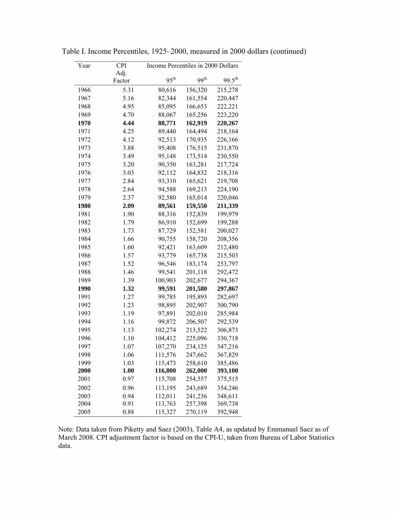
Table I. Income Percentiles, 1925–2000, measured in 2000 dollars (continued)

Year CPI Adj.

Income Percentiles in 2000 Dollars

Factor 95th 99th 99.5th

1966 5.31 80,616 156,320 215,278 1967 5.16 82,344 161,554 220,447 1968 4.95 85,095 166,653 222,221 1969 4.70 88,067 165,256 223,220 1970 4.44 88,771 162,919 220,267 1971 4.25 89,440 164,494 218,164 1972 4.12 92,513 170,935 226,166 1973 3.88 95,408 176,515 231,870 1974 3.49 95,148 173,514 230,550 1975 3.20 90,350 163,281 217,724 1976 3.03 92,112 164,832 218,316 1977 2.84 93,310 165,621 219,708 1978 2.64 94,588 169,213 224,190 1979 2.37 92,580 165,014 220,046 1980 2.09 89,561 159,550 211,339 1981 1.90 88,316 152,839 199,979 1982 1.79 86,910 152,699 199,288 1983 1.73 87,729 152,581 200,027 1984 1.66 90,755 158,720 208,356 1985 1.60 92,421 163,609 212,480 1986 1.57 93,779 165,738 215,503 1987 1.52 96,546 183,174 253,797 1988 1.46 99,541 201,118 292,472 1989 1.39 100,903 202,677 294,367 1990 1.32 99,591 201,580 297,867 1991 1.27 99,785 195,893 282,697 1992 1.23 98,895 202,907 300,790 1993 1.19 97,891 202,010 285,984 1994 1.16 99,872 206,507 292,539 1995 1.13 102,274 213,522 306,873 1996 1.10 104,412 225,096 330,718 1997 1.07 107,270 234,125 347,216 1998 1.06 111,576 247,662 367,829 1999 1.03 115,473 258,610 385,486 2000 1.00 116,800 262,000 393,100 2001 0.97 115,708 254,557 375,515

2002 0.96 113,195 243,689 354,246 2003 0.94 112,011 241,236 348,611 2004 0.91 113,763 257,398 369,738 2005 0.88 115,327 270,119 392,948

Note: Data taken from Piketty and Saez (2003), Table A4, as updated by Emmanuel Saez as of March 2008. CPI adjustment factor is based on the CPI-U, taken from Bureau of Labor Statistics data.

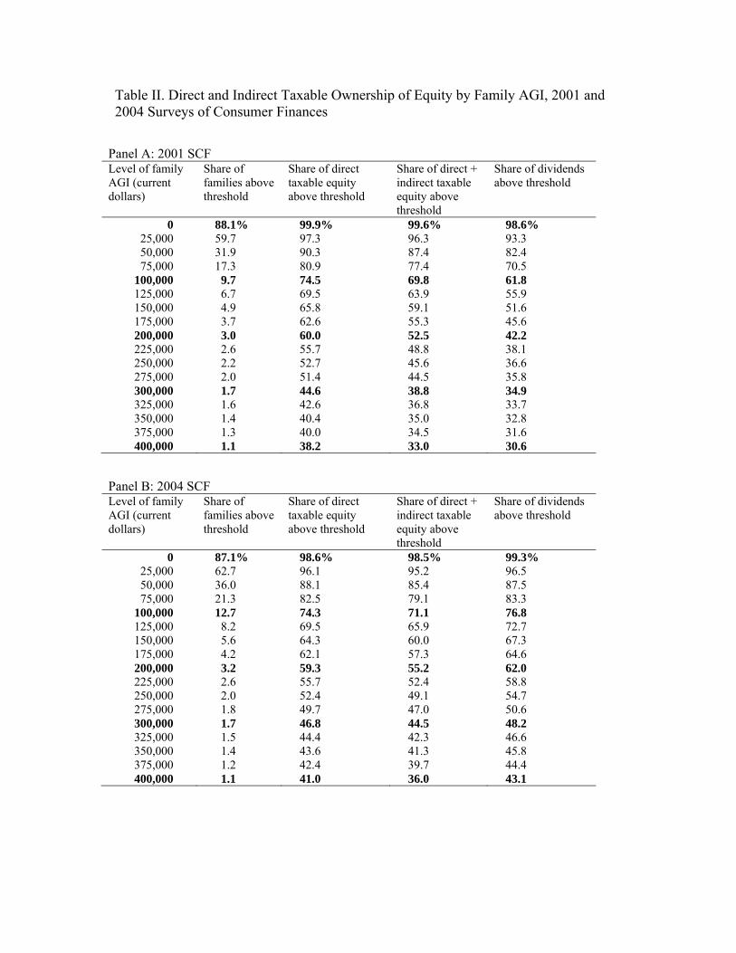
Table II. Direct and Indirect Taxable Ownership of Equity by Family AGI, 2001 and 2004 Surveys of Consumer Finances

Panel A: 2001 SCF Level of family AGI (current dollars)

Share of families above threshold

Share of direct taxable equity above threshold

Share of direct + indirect taxable equity above threshold

Share of dividends above threshold

0 88.1% 99.9% 99.6% 98.6% 25,000 59.7 97.3 96.3 93.3 50,000 31.9 90.3 87.4 82.4 75,000 17.3 80.9 77.4 70.5

100,000 9.7 74.5 69.8 61.8 125,000 6.7 69.5 63.9 55.9 150,000 4.9 65.8 59.1 51.6 175,000 3.7 62.6 55.3 45.6 200,000 3.0 60.0 52.5 42.2 225,000 2.6 55.7 48.8 38.1 250,000 2.2 52.7 45.6 36.6 275,000 2.0 51.4 44.5 35.8 300,000 1.7 44.6 38.8 34.9 325,000 1.6 42.6 36.8 33.7 350,000 1.4 40.4 35.0 32.8 375,000 1.3 40.0 34.5 31.6 400,000 1.1 38.2 33.0 30.6

Panel B: 2004 SCF Level of family AGI (current dollars)

Share of families above threshold

Share of direct taxable equity above threshold

Share of direct + indirect taxable equity above threshold

Share of dividends above threshold

0 87.1% 98.6% 98.5% 99.3% 25,000 62.7 96.1 95.2 96.5 50,000 36.0 88.1 85.4 87.5 75,000 21.3 82.5 79.1 83.3

100,000 12.7 74.3 71.1 76.8 125,000 8.2 69.5 65.9 72.7 150,000 5.6 64.3 60.0 67.3 175,000 4.2 62.1 57.3 64.6 200,000 3.2 59.3 55.2 62.0 225,000 2.6 55.7 52.4 58.8 250,000 2.0 52.4 49.1 54.7 275,000 1.8 49.7 47.0 50.6 300,000 1.7 46.8 44.5 48.2 325,000 1.5 44.4 42.3 46.6 350,000 1.4 43.6 41.3 45.8 375,000 1.2 42.4 39.7 44.4 400,000 1.1 41.0 36.0 43.1

Table III. Overview of Investment Tax Implications

This table summarizes the U.S. federal taxation of investment income for individual investors since 1927. Data from IRS Statistics of Income publications, from Burman (1999), from Poterba and Weisbenner (2003), Shackelford (2000) and Barclay, Holderness, and Sheehan (2003). From 1933 to 1941 capital gains taxes were assessed at ordinary income tax rates, with up to 50% (1938–1941) or 70% (1933–1937) of the capital gains excluded from income, depending on holding period. During 1997, a medium-term rate for holding periods of greater than 12 months and less than 18 months was temporarily instituted.

Panel A: 1927–1953

1927–1933 1934–1941 1942–1953

Max. Ordinary Income Rate

1927–1928: 25% 1929: 24% 1930: 25% 1931: 24% 1932: 42% 1933: 38%

1934: 43% 1935: 49% 1936–1937: 62% 1938: 47% 1939: 55% 1940: 60% 1941: 69%

1942–1943: 85% 1944: 92% 1945: 90% 1946–1947: 84.6% 1948–1949: 68.6% 1950: 68.25% 1951: 82% 1952–1953: 80%

Dividends

Ordinary income

Ordinary income

Ordinary income

Long-Term Capital Gain/Loss

12.5%

Ordinary income minus 1933–1937: 70% 1938–1941: 50%

Ordinary income minus 50%

Medium-Term Capital Gain/Loss

None

None

None

Short-Term Capital Gain/Loss

Ordinary income

Ordinary income

Ordinary income

Table III. Overview of Investment Tax Implications

Panel B: 1954–1996

1954–1969 1970–1986 1987–1996

Max. Ordinary Income Rate

1954–1963: 78% 1964: 68.5% 1965: 64% 1966–1967: 68% 1968: 74.175% 1969: 14.8%

1970: 71.75% 1971–1981: 70% 1982–1986: 50%

1987: 38.5% 1988–1990: 28% 1991–1992: 31% 1993: 36% 1994–1996: 39.6%

Dividends

Ordinary income

Ordinary income

Ordinary income

Long-Term Capital Gain/Loss

Ordinary income minus 50%

1970–1978: Ordinary income minus 50%

1979–1986: Ordinary income minus 60%

28% max.

Medium-Term Capital Gain/Loss

None

None

None

Short-Term Capital Gain/Loss

Ordinary income

Ordinary income

1987: Ordinary income 1988–1990: 28% max. 1991–1992: 31% max. 1993–1996: Ordinary income

Table III. Overview of Investment Tax Implications

Panel C: 1997–2007

1997 1998–2002 2003–2007

Max. Ordinary Income Rate

39.6%

1998–2001: 39.6% 2002: 38.6% 2003: 35%

35%

Dividends

Ordinary income

Ordinary income

Tax rates 5% and 15%

Long-Term Capital Gain/Loss

28% max. before or on May 6 20% max. after May 6

20% max 2001–2002: 20% or 18% for 5-year holding periods. 2003: 15% max

2003: 15% max

Medium-Term Capital Gain/Loss

28%

None

None

Short-Term Capital Gain/Loss

Ordinary income

Ordinary income

Ordinary income

Table IV, Panel A. Tax Impact of Long Strategies Using Time-Appropriate Tax Rates

Sample period is 6/1927–6/2007. Assumes investors have immediate use of net realized losses. Dividend yield and turnover correspond to the dividend yield and turnover of the portfolio of a tax-exempt investor. Return is the average annualized log return, which is computed by multiplying 12 times the log of Effective Value dividend by last month’s Effective Value, where Effective Value = Liquidation Value + 0.193*(Nominal Value – Liquidation Value). CG Effective Tax Rate is the percentage difference between the after-tax return and the return of a taxed portfolio that reinvests dividend taxes that would have otherwise been paid. Div Tax Cost is the percentage difference between the after-tax return and the return of a taxed portfolio that reinvests capital gains taxes that would have otherwise been paid. Effective Tax Rate is the percentage loss of taxable return relative to the tax-exempt return.

Strategy Tax Individual Income Level Percentile (dividend yield, turnover) Exempt 95 99 99.5 99.5+NY

S & P (3.91, 4.13)

After-tax Return 9.65 8.44 8.10 7.89 7.58 Avg Overhang 7.52 9.02 9.85 12.16 CG Effective Tax Rate 2.45 2.51 2.52 3.45 Div Effective Tax Rate 9.76 13.11 15.14 17.20 Total Effective Tax Rate 12.51 16.08 18.24 21.48

VWRET (3.90, 3.98)

After-tax Return 9.79 8.59 8.24 8.04 7.73 Avg Overhang 3.91 3.91 3.91 3.91 CG Effective Tax Rate 2.37 2.40 2.40 3.25 Div Effective Tax Rate 9.59 12.90 14.91 16.88 Total Effective Tax Rate 12.28 15.80 17.94 21.09

EWRET (3.57, 44.76)

After-tax Return 12.28 10.57 10.09 9.77 9.36 Avg Overhang 5.38 6.81 7.71 9.44 CG Effective Tax Rate 6.38 7.60 8.42 10.08 Div Effective Tax Rate 7.22 9.71 11.26 12.76 Total Effective Tax Rate 13.92 17.84 20.39 23.74

No Div (0.56, 31.50)

After-tax Return 7.98 7.17 7.04 6.89 6.64 Avg Overhang 3.60 4.26 4.73 5.78 CG Effective Tax Rate 8.82 9.75 11.19 13.95 Div Effective Tax Rate 1.32 1.94 2.38 3.13 Total Effective Tax Rate 10.17 11.74 13.64 16.73

Low Div (3.98, 6.81)

After-tax Return 9.78 8.58 8.24 8.03 7.73 Avg Overhang 3.99 3.99 3.99 3.99 CG Effective Tax Rate 2.18 2.03 2.00 2.67 Div Effective Tax Rate 9.73 13.08 15.09 17.09 Total Effective Tax Rate 12.26 15.70 17.87 20.95

High Div (5.46, 30.48)

After-tax Return 12.43 10.31 9.75 9.39 8.87 Avg Overhang 3.00 3.77 4.28 5.25 CG Effective Tax Rate 6.25 7.20 7.87 9.77 Div Effective Tax Rate 10.53 13.94 16.01 18.27 Total Effective Tax Rate 17.01 21.53 24.40 28.65

Risk-Free Bill

After-tax Return 3.68 2.52 2.22 2.08 1.87 Total Effective Tax Rate 31.56 39.58 43.55 49.20

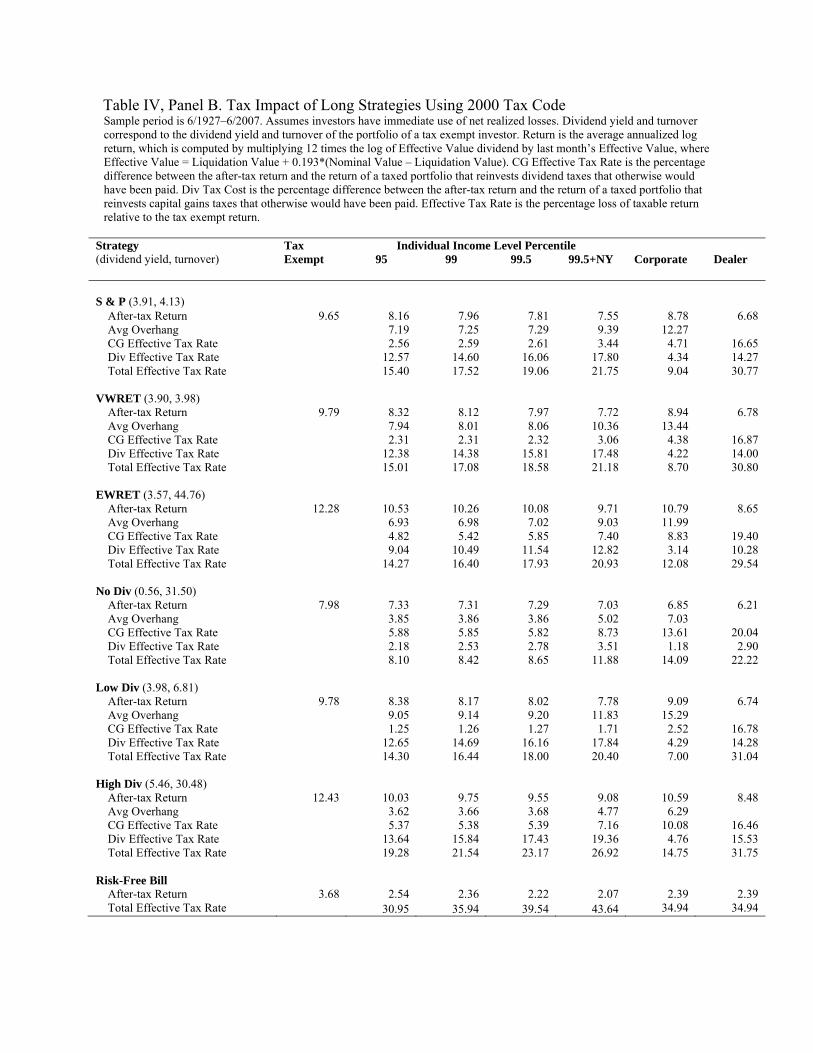
Table IV, Panel B. Tax Impact of Long Strategies Using 2000 Tax Code Sample period is 6/1927–6/2007. Assumes investors have immediate use of net realized losses. Dividend yield and turnover correspond to the dividend yield and turnover of the portfolio of a tax exempt investor. Return is the average annualized log return, which is computed by multiplying 12 times the log of Effective Value dividend by last month’s Effective Value, where Effective Value = Liquidation Value + 0.193*(Nominal Value – Liquidation Value). CG Effective Tax Rate is the percentage difference between the after-tax return and the return of a taxed portfolio that reinvests dividend taxes that otherwise would have been paid. Div Tax Cost is the percentage difference between the after-tax return and the return of a taxed portfolio that reinvests capital gains taxes that otherwise would have been paid. Effective Tax Rate is the percentage loss of taxable return relative to the tax exempt return.

Strategy Tax Individual Income Level Percentile (dividend yield, turnover) Exempt 95 99 99.5 99.5+NY Corporate Dealer

S & P (3.91, 4.13)

After-tax Return 9.65 8.16 7.96 7.81 7.55 8.78 6.68 Avg Overhang 7.19 7.25 7.29 9.39 12.27 CG Effective Tax Rate 2.56 2.59 2.61 3.44 4.71 16.65 Div Effective Tax Rate 12.57 14.60 16.06 17.80 4.34 14.27 Total Effective Tax Rate 15.40 17.52 19.06 21.75 9.04 30.77

VWRET (3.90, 3.98)

After-tax Return 9.79 8.32 8.12 7.97 7.72 8.94 6.78 Avg Overhang 7.94 8.01 8.06 10.36 13.44 CG Effective Tax Rate 2.31 2.31 2.32 3.06 4.38 16.87 Div Effective Tax Rate 12.38 14.38 15.81 17.48 4.22 14.00 Total Effective Tax Rate 15.01 17.08 18.58 21.18 8.70 30.80

EWRET (3.57, 44.76)

After-tax Return 12.28 10.53 10.26 10.08 9.71 10.79 8.65 Avg Overhang 6.93 6.98 7.02 9.03 11.99 CG Effective Tax Rate 4.82 5.42 5.85 7.40 8.83 19.40 Div Effective Tax Rate 9.04 10.49 11.54 12.82 3.14 10.28 Total Effective Tax Rate 14.27 16.40 17.93 20.93 12.08 29.54

No Div (0.56, 31.50)

After-tax Return 7.98 7.33 7.31 7.29 7.03 6.85 6.21 Avg Overhang 3.85 3.86 3.86 5.02 7.03 CG Effective Tax Rate 5.88 5.85 5.82 8.73 13.61 20.04 Div Effective Tax Rate 2.18 2.53 2.78 3.51 1.18 2.90 Total Effective Tax Rate 8.10 8.42 8.65 11.88 14.09 22.22

Low Div (3.98, 6.81)

After-tax Return 9.78 8.38 8.17 8.02 7.78 9.09 6.74 Avg Overhang 9.05 9.14 9.20 11.83 15.29 CG Effective Tax Rate 1.25 1.26 1.27 1.71 2.52 16.78 Div Effective Tax Rate 12.65 14.69 16.16 17.84 4.29 14.28 Total Effective Tax Rate 14.30 16.44 18.00 20.40 7.00 31.04

High Div (5.46, 30.48)

After-tax Return 12.43 10.03 9.75 9.55 9.08 10.59 8.48 Avg Overhang 3.62 3.66 3.68 4.77 6.29 CG Effective Tax Rate 5.37 5.38 5.39 7.16 10.08 16.46 Div Effective Tax Rate 13.64 15.84 17.43 19.36 4.76 15.53 Total Effective Tax Rate 19.28 21.54 23.17 26.92 14.75 31.75

Risk-Free Bill

After-tax Return 3.68 2.54 2.36 2.22 2.07 2.39 2.39 Total Effective Tax Rate 30.95 35.94 39.54 43.64 34.94 34.94

Table V, Panel A. Tax Impact of Style Strategies Using Time Appropriate Tax Rates

Sample period is 6/1927–6/2007. Assumes investors have immediate use of net realized losses. Dividend yield and turnover correspond to the dividend yield and turnover of the portfolio of a tax exempt investor. Return is the average annualized log return, which is computed by multiplying 12 times the log of Effective Value dividend by last month’s Effective Value, where Effective Value = Liquidation Value + 0.193*(Nominal Value – Liquidation Value). CG Effective Tax Rate is the percentage difference between the after-tax return and the return of a taxed portfolio that reinvests dividend taxes that otherwise would have been paid. Div Tax Cost is the percentage difference between the after-tax return and the return of a taxed portfolio that reinvests capital gains taxes that otherwise would have been paid. Effective Tax Rate is the percentage loss of taxable return relative to the tax exempt return.

Strategy Tax Individual Income Level Percentile (dividend yield, turnover) Exempt 95 99 99.5 99.5+NY

Large (3.92, 5.56)

After-tax Return 9.40 8.25 7.93 7.72 7.43 Avg Overhang 8.19 9.98 10.99 13.53 CG Effective Tax Rate 1.68 1.41 1.31 1.88 Div Effective Tax Rate 10.08 13.53 15.61 17.65 Total Effective Tax Rate 12.19 15.64 17.81 20.89

Growth (3.22, 18.27)

After-tax Return 8.86 7.72 7.43 7.23 6.93 Avg Overhang 6.77 8.42 9.42 11.51 CG Effective Tax Rate 4.32 4.33 4.51 5.76 Div Effective Tax Rate 8.05 10.99 12.83 14.50 Total Effective Tax Rate 12.84 16.10 18.34 21.71

Small (2.84, 40.13)

After-tax Return 11.97 10.00 9.47 9.13 8.66 Avg Overhang 0.23 0.30 0.48 0.55 CG Effective Tax Rate 10.02 12.21 13.64 16.36 Div Effective Tax Rate 6.48 8.61 9.96 11.36 Total Effective Tax Rate 16.52 20.88 23.73 27.66

Value (4.03, 43.24)

After-tax Return 12.63 10.31 9.72 9.35 8.85 Avg Overhang 1.95 2.40 2.75 3.29 CG Effective Tax Rate 9.17 10.90 12.02 14.20 Div Effective Tax Rate 9.01 11.85 13.59 15.06 Total Effective Tax Rate 18.37 23.05 26.02 29.92

Momentum (3.31, 365.36)

After-tax Return 14.04 11.40 10.68 10.21 9.64 Avg Overhang 1.72 2.17 2.43 2.76 CG Effective Tax Rate 13.35 16.49 18.62 21.48 Div Effective Tax Rate 5.36 7.30 8.48 9.59 Total Effective Tax Rate 18.81 23.94 27.30 31.32

Table V, Panel B. Tax Impact of Style Strategies Using 2000 Tax Code

Sample period is 6/1927–6/2007. Assumes investors have immediate use of net realized losses. Dividend yield and turnover correspond to the dividend yield and turnover of the portfolio of a tax exempt investor. Return is the average annualized log return, which is computed by multiplying 12 times the log of Effective Value dividend by last month’s Effective Value, where Effective Value = Liquidation Value + 0.193*(Nominal Value – Liquidation Value). CG Effective Tax Rate is the percentage difference between the after-tax return and the return of a taxed portfolio that reinvests dividend taxes that otherwise would have been paid. Div Tax Cost is the percentage difference between the after-tax return and the return of a taxed portfolio that reinvests capital gains taxes that otherwise would have been paid. Effective Tax Rate is the percentage loss of taxable return relative to the tax exempt return.

Strategy Tax Individual Income Level Percentile (dividend yield, turnover) Exempt 95 99 99.5 99.5+NY Corporate Dealer

Large (3.92, 5.56)

After-tax Return 9.40 8.07 7.87 7.72 7.50 8.79 6.50 Avg Overhang 8.97 9.05 9.11 11.72 15.17 CG Effective Tax Rate 0.69 0.70 0.70 1.05 1.89 16.24 Div Effective Tax Rate 12.97 15.07 16.57 18.28 4.39 14.63 Total Effective Tax Rate 14.08 16.28 17.87 20.21 6.49 30.87

Growth (3.22, 18.27)

After-tax Return 8.86 7.66 7.49 7.37 7.13 8.04 6.18 Avg Overhang 8.37 8.42 8.46 10.81 14.31 CG Effective Tax Rate 1.63 1.62 1.61 2.54 4.99 17.49 Div Effective Tax Rate 11.28 13.11 14.42 15.87 3.78 12.70 Total Effective Tax Rate 13.47 15.38 16.76 19.53 9.17 30.26

Small (2.84, 40.13)

After-tax Return 11.97 9.83 9.68 9.57 9.10 9.70 8.78 Avg Overhang -0.62 -0.62 -0.62 -0.53 -0.20 CG Effective Tax Rate 10.51 10.58 10.63 13.50 16.65 18.53 Div Effective Tax Rate 7.37 8.56 9.41 10.62 2.73 8.55 Total Effective Tax Rate 17.90 19.17 20.08 23.96 19.00 26.70

Value (4.03, 43.24)

After-tax Return 12.63 10.30 10.09 9.94 9.48 10.43 9.07 Avg Overhang 1.92 1.93 1.94 2.57 3.47 CG Effective Tax Rate 8.36 8.38 8.39 10.63 13.87 17.00 Div Effective Tax Rate 9.90 11.50 12.65 13.81 3.24 11.04 Total Effective Tax Rate 18.47 20.13 21.32 24.95 17.41 28.22

Momentum (3.31, 365.36)

After-tax Return 14.04 10.85 10.66 10.51 9.91 10.76 9.64 Avg Overhang 2.21 2.35 2.45 2.83 2.77 CG Effective Tax Rate 15.28 15.46 15.60 18.89 20.83 23.09 Div Effective Tax Rate 7.31 8.49 9.35 10.30 2.46 8.24 Total Effective Tax Rate 22.71 24.10 25.11 29.42 23.37 31.37

Table VI, Panel A. Tax Impact of Long-Short Strategies Using Time Appropriate Tax Rates

Sample period is 6/1927–6/2007. Assumes investors have immediate use of net realized losses. Return is the average annualized log return, which is computed by multiplying 12 times the log of Effective Value dividend by last month’s Effective Value, where Effective Value = Liquidation Value + 0.193*(Nominal Value – Liquidation Value). CG Effective Tax Rate is the percentage difference between the after-tax return and the return of a taxed portfolio that reinvests dividend taxes that otherwise would have been paid. Div Tax Cost is the percentage difference between the after-tax return and the return of a taxed portfolio that reinvests capital gains taxes that otherwise would have been paid. Effective Tax Rate is the percentage loss of taxable return relative to the tax exempt return.

Strategy Tax Individual Income Level Percentile (dividend yield, turnover) Exempt 95 99 99.5 99.5+NY

VWRET-Rf

Total Return 6.11 6.07 6.02 5.96 5.86 Long Return 9.79 8.59 8.24 8.04 7.73 Short Return 3.67 2.51 2.22 2.07 1.86 Long Turnover 3.98 4.20 4.26 4.30 4.35 Short Turnover CG Effective Tax Rate 3.79 3.83 3.82 5.18 Div Effective Tax Rate -3.64 -3.17 -2.34 -2.58

Effective Tax Rate 0.66 1.46 2.50 4.15 SMB

Total Return 2.11 1.97 1.90 1.84 1.77 Long Return 11.96 10.05 9.56 9.23 8.77 Short Return 10.47 8.48 7.96 7.64 7.17 Long Turnover 35.75 36.36 36.49 36.56 36.77 Short Turnover 17.92 17.86 17.76 17.70 17.57 CG Effective Tax Rate 13.32 18.62 22.14 26.66 Div Effective Tax Rate -6.59 -8.42 -9.13 -10.36

Effective Tax Rate 6.55 9.92 12.69 15.86 HML

Total Return 3.59 2.98 2.80 2.68 2.56 Long Return 12.76 10.49 9.93 9.55 9.06 Short Return 9.67 7.98 7.53 7.24 6.82 Long Turnover 42.79 43.43 43.57 43.64 43.77 Short Turnover 36.48 36.21 36.07 35.99 35.89 CG Effective Tax Rate 7.79 10.70 12.75 14.92 Div Effective Tax Rate 9.05 11.02 12.05 12.87 Effective Tax Rate 17.02 22.02 25.19 28.68

Table VI, Panel B. Tax Impact of Long-Short Strategies Using 2000 Tax Code

Sample period is 6/1927–6/2007. Assumes investors have immediate use of net realized losses. Return is the average annualized log return, which is computed by multiplying 12 times the log of Effective Value dividend by last month’s Effective Value, where Effective Value = Liquidation Value + 0.193*(Nominal Value – Liquidation Value). CG Effective Tax Rate is the percentage difference between the after-tax return and the return of a taxed portfolio that reinvests dividend taxes that otherwise would have been paid. Div Tax Cost is the percentage difference between the after-tax return and the return of a taxed portfolio that reinvests capital gains taxes that otherwise would have been paid. Effective Tax Rate is the percentage loss of taxable return relative to the tax exempt return.

Strategy Tax Individual Income Level Percentile Corporate Dealer

Exempt 95 99 99.5 99.5+NY

VWRET-Rf

Total Return 6.11 5.78 5.76 5.75 5.64 5.65 4.38

Long Return 9.79 8.32 8.12 7.97 7.72 8.94 6.78

Short Return 3.67 2.54 2.35 2.22 2.07 3.29 2.39 Long Turnover 3.98 4.25 4.29 4.32 4.36 4.15

Short Turnover

CG Effective Tax Rate 3.68 3.69 3.69 4.88 6.99 27.03

Div Effective Tax Rate 1.21 1.40 1.55 1.75 0.46 1.40

Effective Tax Rate 5.41 5.73 5.97 7.67 7.61 28.32

SMB

Total Return 2.11 1.81 1.82 1.83 1.78 1.60 1.49

Long Return 11.96 9.88 9.68 9.55 9.12 10.01 8.51

Short Return 10.47 8.18 7.97 7.81 7.36 8.29 7.29

Long Turnover 35.75 36.49 36.55 36.60 36.81 36.32 Short Turnover 17.92 17.68 17.67 17.67 17.49 17.36

CG Effective Tax Rate 21.16 21.71 22.10 25.72 26.58 37.14

Div Effective Tax Rate -6.92 -8.03 -8.84 -9.65 -2.26 -7.71

Effective Tax Rate 14.07 13.47 13.02 15.65 24.08 29.28

HML

Total Return 3.59 2.92 2.90 2.89 2.76 2.74 2.50

Long Return 12.76 10.47 10.26 10.11 9.65 10.57 9.07

Short Return 9.67 7.68 7.49 7.34 6.95 7.81 6.80

Long Turnover 42.79 43.51 43.58 43.63 43.74 43.31 Short Turnover 36.48 35.95 35.95 35.95 35.82 35.51

CG Effective Tax Rate 13.09 12.62 12.28 15.08 21.42 24.21

Div Effective Tax Rate 5.31 6.17 6.79 7.13 1.46 5.64

Effective Tax Rate 18.71 19.15 19.46 23.08 23.63 30.42

Table VII. Importance of Loss Realization Rules

Sample period is 6/1927–6/2007. Comparison of effective tax rates of portfolios depending on whether investors immediately use realized losses or whether losses are carried forward to future periods. Effective Tax Rate is the annualized percentage loss of taxable return relative to the tax-exempt return.

Strategy (dividend yield, turnover)

Effective Tax Rate—Carry Forward Losses (Effective Tax Rate—Use Losses Immediately)

[Difference]

99th Percentile Individual Corporate

Actual Code 2000 Code 2000 Code

S & P (3.91, 4.13)

16.37 (16.08) [0.29]

18.26 (17.52) [0.73]

10.21 (9.04) [1.17]

VWRET (3.90, 3.98)

16.06 (15.80) [0.26]

17.76 (17.08) [0.68]

9.78 (8.70) [1.08]

EWRET (3.57, 44.76)

18.93 (17.44) [1.08]

20.08 (16.04) [3.69]

17.08 (14.09) [5.00]

No Div (0.56, 31.50)

15.58 (11.74) [3.84]

16.51 (8.42) [8.09]

24.06 (14.41) [9.97]

Low Div (3.98, 6.81)

16.27 (15.70) [0.58]

18.12 (16.44) [1.68]

9.97 (7.00) [2.77]

High Div (5.46, 30.48)

22.66 (21.53) [1.13]

24.39 (21.54) [2.85]

18.45 (14.87) [3.70]

Large (3.92, 5.56)

16.51 (15.64) [0.87]

18.26 (16.28) [1.98]

9.62 (6.49) [3.14]

Growth (3.22, 18.27)

17.74 (16.10) [1.64]

19.65 (15.38) [4.27]

14.88 (9.17) [5.71]

Small (2.84, 40.13)

24.92 (20.88) [4.03]

25.75 (19.17) [6.58]

25.40 (19.00) [6.39]

Value (4.03, 43.24)

25.33 (23.05) [2.28]

24.84 (20.13) [4.71]

22.09 (17.41) [4.68]

Momentum (3.31, 365.36)

27.53 (23.94)

[3.59]

28.40 (24.10) [4.31]

27.44 (23.37) [4.07]

Table VIII. Tax Benefit of Basis Allocation and Tax-Timing Strategies

Sample period is 6/1927–6/2007. Assumes investors have immediate use of net realized losses. This table presents the returns and relative advantage of the various capital gains realization strategies for an investor with an adjusted gross income in the 99 percentile. The strategies, from left to right, correspond to least tax advantaged to most tax advantaged. Dividend yield and turnover correspond to the dividend yield and turnover of the portfolio of a tax exempt investor. The percentage benefit is calculated as the average log return of the optimal divided by the average log return of the suboptimal strategy, minus one. All returns are expressed as annualized by multiplying by 12. The optimal strategy is to sell the highest-basis shares first, and the suboptimal strategy is to sell the lowest-basis shares first.

Using Tax Rates That Correspond to the Return Period Using Tax Rates That Correspond to the 2000 Tax Code

Strategy (dividend yield, turnover)

Sell lowest basis first,

harvest gains

(1)

Sell lowest basis first

Sell highest basis first

Sell highest basis first,

harvest losses

Sell lowest basis first,

harvest gains

(1)

Sell lowest basis first

Sell highest basis first

Sell highest basis first,

harvest losses

S & P (3.91, 4.13) 5.83 7.97 8.24 8.67 5.43 7.74 7.96 8.91

Return minus strategy (1) return 2.14 2.41 2.84 2.31 2.53 3.48 % improvement above strategy (1) 36.71 41.33 48.71 42.54 46.59 64.09

Growth (3.22, 18.27) 5.09 7.21 7.43 7.95 4.95 7.22 7.49 8.23 Return minus strategy (1) return 2.45 2.68 3.30 2.27 2.54 3.28 % improvement above strategy (1) 53.80 59.00 72.52 45.86 51.31 66.26

Small (2.84, 40.13) 6.75 9.25 9.47 11.06 6.74 9.35 9.68 11.81 Return minus strategy (1) return 2.88 3.13 4.96 2.61 2.94 5.07 % improvement above strategy (1) 47.88 52.08 82.66 38.72 43.62 75.22

Value (4.03, 43.24) 7.36 9.52 9.72 10.81 7.50 9.79 10.09 11.59 Return minus strategy (1) return 2.50 2.72 3.99 2.29 2.59 4.09 % improvement above strategy (1) 37.79 41.14 60.31 30.53 34.53 54.53