Investment risk-sharing

A State-of-the-Art Report

Rami Chehab∗ and Catherine Donnelly†

https://risk-insight-lab.com/

Risk Insight Lab,Department of Actuarial Mathematics and Statistics,

Heriot-Watt University, Edinburgh, Scotland EH14 4AS

29 May 2018

This work was funded by the Actuarial Research Centre (ARC) of The Institute andFaculty of Actuaries (IFoA), UK.

Disclaimer: The views expressed in this publication are those of the authors and notnecessarily those of the IFoA. The IFoA do not endorse any of the views stated, norany claims or representations made in this publication and accept no responsibility orliability to any person for loss or damage suffered as a consequence of their placingreliance upon any view, claim or representation made in this publication. The informa-tion and expressions of opinion contained in this publication are not intended to be acomprehensive study, nor to provide actuarial advice or advice of any nature and shouldnot be treated as a substitute for specific advice concerning individual situations.

Please cite this report as: Chehab, R. and Donnelly, C. (2018). Investment risk-sharing: A State-of-the-Art Report. Technical report number 2, Risk Insight Lab,Heriot-Watt University, UK. https://risk-insight-lab.com/outputs/

∗R.Chehab@hw.ac.uk†C.Donnelly@hw.ac.uk

1

ForewordThe authors are part of the ARC research project “Minimising Longevity and Investment Riskwhile Optimising Future Pension Plans”. The goal is to develop new pension product designs thatkeep the customers’ needs at the forefront. As a first step, this report was written to familiarizethe project team with the existing knowledge on decumulation strategies.

The key question that we sought to answer is: “What structures in the pension arena havebeen proposed for investment risk-sharing?”. The structures cover participating policies (or with-profits contracts), defined benefit pension plans and collective defined contribution plans as wellas theoretical structures which have proposed in the literature.

Contents1 Executive summary 3

2 Introduction 4

3 Participating policies 53.1 Terminology . . . . . . . . . . . . . . . . . . . . . . . . . . . . . . . . . . . . . . . . 53.2 Financial market models . . . . . . . . . . . . . . . . . . . . . . . . . . . . . . . . . 63.3 Contracts with a minimum guarantee . . . . . . . . . . . . . . . . . . . . . . . . . 7

3.3.1 (Investment) return-based distribution . . . . . . . . . . . . . . . . . . . . . 73.3.2 Reserve-based distribution . . . . . . . . . . . . . . . . . . . . . . . . . . . . 93.3.3 An inter-generational contract with a minimum guarantee . . . . . . . . . . 123.3.4 Different frameworks for defining bankruptcy . . . . . . . . . . . . . . . . . 13

3.4 Contracts without a minimum guarantee . . . . . . . . . . . . . . . . . . . . . . . . 15

4 Funded, collective pension plans 234.1 Defined benefit (DB) plans . . . . . . . . . . . . . . . . . . . . . . . . . . . . . . . 234.2 Collective defined contribution (CDC) plans . . . . . . . . . . . . . . . . . . . . . . 244.3 Analyses of inter-generational risk-sharing in private pension plans . . . . . . . . . 24

5 Theoretical risk-sharing frameworks 275.1 Financial fairness and Pareto-efficiency . . . . . . . . . . . . . . . . . . . . . . . . . 27

5.1.1 One-period model . . . . . . . . . . . . . . . . . . . . . . . . . . . . . . . . 275.1.2 Multi-period model . . . . . . . . . . . . . . . . . . . . . . . . . . . . . . . . 28

6 Conclusion 34

2

1 Executive summaryInvestment risk-sharing is a means of sharing money among a collection of people, companiesand institutions. It can happen at a point in time or over a period of time. Here the focusis on investment risk-sharing in the context of saving and spending money for retirement. Themotivation for risk-sharing is to improve the welfare of the participants.

There is relatively little in the literature on different risk-sharing mechanisms. Much of it focuseson the analysis of collective schemes where the risk-sharing is enabled by a shared fund. Fundedpension schemes, where the shared fund is the entire fund, and participating policies, where theshared fund is a buffer account separate to individual customer accounts, fall under this category.

Participating policies are investment products which share investment returns among policyhold-ers. Many of them incorporate a minimum guaranteed return. They may include inter-generationalrisk-sharing between policyholders via a buffer account. Policyholders have individual accountsand, in the case of inter-temporal risk-sharing, may have a claim on a shared account called abuffer. However, many policies – as described in the literature – do not and it is the insurancecompany who is responsible for the buffer.

Collective defined contribution schemes allow for inter-generational risk-sharing. Defined benefitpension plans may include a small element of it. There are no individual account values or bufferaccount in funded pension schemes. Instead, the entire fund represents the totality of the members’claims on the fund. Collective defined contribution schemes are shown to be welfare-improving inseveral papers, compared to the members investing individually.

Several authors have solved for risk-sharing mechanism that share money among the participantsin a financially-fair and Pareto-efficient way. The motivations and set-ups of the authors can bedifferent, and they don’t all translate easily into the retirement context. The mechanisms arecurrently too abstract to be considered as useful in a practical setting. The rules for allocatingmoney are calculated from algorithms, which make them difficult to communicate. They rely onassigning a utility function to each agent in the risk-sharing system, which immediately makesthem quite abstract.

3

2 IntroductionInvestment risk-sharing is a means of sharing money among a collection of people, companies andinstitutions. It can happen at a point in time or over a period of time. Here the focus is oninvestment risk-sharing in the context of saving and spending money for retirement.

There are many structures for investment risk-sharing which are observed in practice. For exam-ple, there are products sold by insurance companies, called with-profits or participating policies.There are funded private pension schemes which are generally only open to employees of certaincompanies or industries. These pension schemes and products may share investment values indi-rectly over time among a group of people. However, they don’t all utilize investment risk-sharing.For many, the insurance company or the sponsoring employers alone assume the risk of meetingany guarantees. These structures are presented in Sections 3 and 4.

Where there is investment risk-sharing, a common feature is the existence of a buffer. For newentrants to a pension scheme, or new customers, the value of the buffer is a distorted reflectionof the previously experienced investment history. If returns have been good, the buffer should belarge. If returns have been poor, the buffer should be small and perhaps even negative. The bufferallows participants to access historical returns, for the time before they were participants, as wellas for the time during which they are participants.

The buffer is used to smooth the investment values of, or the income paid out to, the participants.If current investment returns are poor, money may be withdrawn from the buffer and distributedamong the current participants. If current returns are high, some of the return may be depositedin the buffer rather than being allocated to the current participants.

Inter-generational fairness is often mentioned in the context of risk-sharing schemes. It is oftennot considered explicitly when setting up a scheme. The rules for allocating values among membersdo not necessarily involve any consideration of inter-generational fairness.

One way of defining fairness is to have a contract which is financially fair at the outset, in thatthe expected discounted value of benefits received equals the discounted value of contributionspaid by the individual at the start of a contract or pension plan membership. On top of this,fairness could also mean that the risk faced by the individual of receiving less than their expectedor promised benefits is equal across all generations.

However, despite investment risk-sharing being relatively common, few methods of sharing re-turns incorporate explicitly a notion of inter-generational fairness. The closest are the Pareto-efficient and financially fair methods outlined in Section 5. However, it is difficult to see how themethods could be communicated and applied easily in practice.

Lots of economics papers have focused on studying whether risk-sharing is welfare-improving tosociety. For example, Beetsma et al. (2012) studied the feasibility and welfare consequences of afunded pension scheme, which has inter-generational risk-sharing, when participation is voluntary.Gollier (2008) also consider funded pension schemes which involved inter-generational risk-sharing.Both papers concluded that risk-sharing is indeed welfare-enhancing.

4

3 Participating policiesParticipating policies, also called with-profits policies, are the focus of this section. They areprimarily a long-term investment contract, as opposed to an insurance contract. The policyholderpays either a single premium at the initiation of the contract, or they pay regular premiums.The premiums are invested by the insurance company. From the policyholder’s perspective, thepremiums accumulate as a function of the underlying investment returns. Participating policiesare a common product in many countries.

There are two common features which are often seen in these contracts. One is a minimum guar-anteed interest rate at which the policyholder’s premium accumulates. The second is a smoothingof the returns granted on the premiums, which is enabled by a buffer.

The focus here is on the underlying mechanisms which allocate the invested monies amongpolicyholders. After introducing some basic terminology, participating policies which have beenstudied in the literature are described. Most of these policies are based on real-life contracts.A notable exception is the contract proposed by Goecke (2013). Although the policyholder canusually surrender the policy before its maturity date in exchange for a payment from the insurancecompany, this option has been ignored in the presentation. Similarly, any insurance benefits paidupon death or ill-health have also been excluded.

Not all of these contracts feature inter-generational risk-sharing. In spite of this, their structureis presented because they may help in proposing new risk-sharing structures which have similar,attractive features.

Few papers analyze specifically either the inter-generational risk-sharing aspect of participatingpolicies. Most papers consider the relationship between a single policyholder and the company.How much should the company charge the policyholder for the policy so that it is fair, i.e. theexpected benefits received by the policyholder are equal to the premiums paid? How much of thebuffer account and the investment returns should be received by the policyholder and how muchby the company?

3.1 Terminology

Customer account with value P

The customer account represents the minimum value paid to the policyholder at the maturity dateof the contract. The policyholder may receive exactly the value of the customer account, or theymay get an additional amount paid to them. The customer account is found on the liabilities sideof a balance sheet of an insurance company. Early surrender is ignored in this report.

The customer may receive a larger value than the customer account value, upon the maturityof their policy. The value of what the customer receives at the maturity time T is denoted L(T ).

Buffer with value B

The primary purpose of the buffer – also called the smoothing account, bonus account or collectivereserve – is to smooth investment returns for customers. It does not belong to a single customer butit belongs to the customers collectively and usually also the company. When investment returnsare poor, money is transferred from the buffer to the individual customer accounts. The oppositemay occur when investment returns are good: money is transferred from the individual customeraccounts to the buffer. Hence the buffer helps to reduce the fluctuations of the financial marketreturns on the customer accounts.

5

The buffer is the account that may enable risk-sharing between the customer and the company,and between the different generations of policyholders. Or it may the responsibility of the companyalone to make good any deficit in the buffer and there is no risk-sharing whatsoever.

Company account with value C

The company account or shareholders’ account, as its name suggests, is the account of the share-holders’ or owners’ of the insurance company that is providing the insurance contract. It is foundon the liability side of the insurance company balance sheet.

Not all of the contracts studied in the literature include a company account. However, wheneverthe insurance company provides guarantees and has a claim on the buffer, it should be understoodthat the buffer account incorporates the company account. Similarly, some of the contracts do notinclude a buffer but do have a company account.

Reference portfolio with value A

Investment return values used for crediting returns to the different accounts are calculated basedon the reference portfolio. The portfolio may represent the actual portfolio holdings backing thepolicy or it may not.

Unless stated otherwise, the initial value A(0) = P (0).

3.2 Financial market models

The most common continuous-time model applied in the literature, the Black-Scholes model, mod-els the price S0 of a risk-free bond as

S0(t) = S0(0)ert (1)

and the price S1 of a risky stock as

S1(t) = S1(0)e(µ−σ2/2)t+σW (t), (2)

at time t ≥ 0, in which the constant r is the risk-free rate of interest, the constant µ is the meanrate of return on the risky stock, the constant σ > 0 is the volatility of return on the risky stockand W is a standard Brownian motion. It is usually assumed that µ > r. The initial prices S0(0)and S1(0) are strictly positive constants.

The Black-Scholes model can easily be extended to include more assets and it is usually astraightforward extension of a derived result to allow for more assets. It is also possible to allowthe parameters r, µ and σ to become deterministic functions or non-trivial stochastic processes.

Due to its structure and properties, the Black-Scholes model is one of the simplest modelsunder which closed-form solutions can be found. Closed-form solutions are very useful. Thesensitivity of the solution to the various parameters can generally be much better understood, andunderstood more quickly, when dealing with a closed-form solution. Moreover, the solution in amore complicated model has often the same broad structure.

Contrast this to trying to understand a solution that is the numerical output of a very com-plicated econometric model, without having the guidance of a solution derived in a simple modellike the Black-Scholes model. There is no help as to what are the important parameters for thesolution. Doing sensitivity testing becomes a difficult task.

The Black-Scholes model is often criticized for not capturing well enough some observed featuresof actual stock-market returns. For example, the probability of extreme returns under the Black-Scholes model is too low, compared to the observed chance of very high or very low returns. It

6

assumes a constant volatility of returns and that returns are independent in non-overlapping timeperiods, which are not observed in practice.

Unless stated otherwise, the Black-Scholes model has been used as the financial market modelin the papers described.

3.3 Contracts with a minimum guarantee

Here participating policies which include a minimum guarantee are described. Effectively, thismeans that the policyholder’s premiums are guaranteed to accumulate at a minimum interest rateby the insurer.

To describe the contracts, the following three accounts are used for the descriptions: a referenceportfolio with value A, the customer account with value P and the buffer with value B. There mayalso be a company account with value C included, or it may be implicitly part of the value of thebuffer. The reference portfolio may be simply a reference index or it may represent the underlyingassets. The policyholder’s contract begins at time 0 and ends at integer time T > 0. Mortalityand surrender are ignored here.

The customer account value P increases at the random policy interest rate rP . The evolution ofrP depends on which contract is being considered. Note that the value of the customer account atthe maturity time T is not necessarily what is paid to the policyholder. To emphasize this point,denote by L(T ) the value of what is paid to the policyholder at the maturity time T .

The buffer is determined residually as

B(n) = A(n)− P (n)− C(n), for n = 1, 2, . . . , T − 1,

and, to allow for L(T ) > P (T ), set B(T ) = A(T )− L(T )− C(T ).

3.3.1 (Investment) return-based distribution

Return-based contracts allocate a return rP to the customer account that is calculated using theannual return of the reference portfolio and a minimum guaranteed interest rate rg. The generalidea is that a percentage of the investment return on the reference portfolio is granted on thecustomer account, subject to a minimum return equal to rg.

Haberman et al. (2003) and Bacinello (2001)

Haberman et al. (2003) consider three smoothing mechanisms in use in the UK.

• Arithmetic average of the last M time period returns, for a constant integer M ≥ 1. For afixed distribution ratio α ≥ 0, the policy interest rate at time n is calculated over the lastm = min{n,M} time periods as

rP (n) = max{rg, α

(1m

[A(n)

A(n− 1) + · · ·+ A(n−m+ 1)A(n−m)

]− 1)}

for n = 1, 2, . . . , T . The customer account value at integer time n ≥ 1 is

P (n) = P0

n∏k=1

(1 + rP (k)) .

Bacinello (2001) studies a similar Italian contract which has M := 1.

7

• Geometric average of the last M time period returns, for a constant integer M ≥ 1. For afixed distribution ratio α ≥ 0, the policy interest rate at time n is calculated over the lastm = min{n,M} time periods as

rP (n) = max{rg, α

((A(n)

A(n−m)

)1/m− 1)}

for n = 1, 2, . . . , T . The customer account value at integer time n is

P (n) = P0

n∏k=1

(1 + rP (k)) .

• Smoothed asset share. For a fixed distribution ratio α ≥ 0, the policy interest rate at time nis

rP (n) = max{rg, α

(A(n)

A(n− 1) − 1)}

,

for n = 1, 2, . . . , T . Here we are obliged to define the unsmoothed asset share (AS), whichaccumulates as

(AS)n = (AS)n−1 (1 + rP (n)) .

The customer account value at integer time n ≥ 1 is

P (n) = β(AS)n + (1− β)P (n− 1),

for a constant weighting factor β ∈ (0, 1).

For the three contracts considered by Haberman et al. (2003), the terminal payout to the policy-holder is

L(T ) = P (T ) + γmax {A(T )− P (T ), 0}

for a participation constant γ ∈ (0, 1). If we could set γ = 1 then the policyholder would receivemax {A(T ), P (T )} at the maturity date. In that case, the customer account value acts as aminimum payout. However, as γ < 1, the policyholder obtains less than the excess value ofthe reference portfolio over the customer account value. To whom does the residual value go? InHaberman et al. (2003), it is the company. The company has guaranteed the minimum annualreturn rg on the policy interest rate, and so it is the company who benefits from any asset out-performance over the customer account value.

Haberman et al. (2003) set the company’s account value to

C(T ) = A(T )− L(T ),

which implies that B(T ) = 0. Haberman et al. (2003) do not describe an explicit buffer. Thissuggests that there is no inter-generational risk-sharing and it is the company who bears anyinvestment risk resulting from the guarantees and smoothing mechanism, through the companyaccount.

The fair value of the contract is the single premium equal to the expected value of the discountedterminal payout P (T ) + γmax {A(T )− P (T ), 0}, calculated under a risk-neutral measure. Haber-man et al. (2003) study the parameter sensitivity of the fair value and other aspects of the threetypes of the contracts.

8

Miltersen and Persson (2003)

Miltersen and Persson (2003) analyze a policy which can model a Norwegian product launched in1998. Their analysis indicates that the Norwegian product is over-priced and they suggest thatmay be the reason the product was not a success. There are similar Danish and Dutch contracts.There is no risk-sharing in this contract as it is described. Instead, the company bears the riskof the investment return being insufficient to pay the minimum interest rate guaranteed on thepolicyholder’s premium.

For the analyzed policy, define the annual investment return process R(n) := A(n)/A(n−1)−1.This may not be the actual investment return achieved by the underlying assets. The customeraccount value is calculated at integer time n is

P (n) = P (n− 1) (1 + rg + αmax {R(n)− rg, 0})× P (n− 1),

with A0 = P0, the initial premium paid by the policyholder. If the investment return in year nsatisfies R(n) > rg, there is an excess monetary return (R(n)−rg)P (n−1). A specified fraction α ofthe excess return is credited to the customer account. Otherwise, if the return satisfies R(n) ≤ rg,there is no excess and the customer account is credited by the amount rgP (n− 1) only.

At the maturity time of the contract, the customer gets P (T ) and the value of the buffer accountif the latter is positive, i.e.

L(T ) = P (T ) + max{B(T ), 0}.

The company’s account value increases as

C(n) = C(n− 1) + βmax {R(n)− rg, 0} × P (n− 1),

with C(0) = 0. If there is an excess monetary return (R(n) − rg)P (n − 1), then the companyaccount is given a fraction β of this amount. Otherwise, if R(n) ≤ rg, there is no excess returnand nothing is credited to or deducted from the company account.

The bonus account is defined residually as B(n) = A(n)−P (n)−C(n). In particular, B(0) = 0.It is possible for the buffer account to have a negative value. For this policy, the company isresponsible for the buffer. The company must cover any deficit in the buffer account at thematurity date of the contract.

Miltersen and Persson (2003) calculate possible values for the triples (rg, α, β) which mean thata single premium is the fair price, under a Black-Scholes model like the one described in Section3.2.

3.3.2 Reserve-based distribution

For reserve-based contracts, returns are distributed to policyholders based on the security of thereserve, as represented by the buffer ratio. The buffer ratio is the size of the buffer B divided bythe customer account value P . There may be a target buffer ratio which must be exceeded beforereturns are paid to a customer account.

The general idea is that a percentage of the buffer ratio above the target buffer ratio is grantedon the customer account, subject to a minimum return equal to rg.

Grosen and Jorgensen (2000)

Grosen and Jorgensen (2000) analyze a reserve-based participating policy. For a target buffer ratioγ ≥ 0, the policy interest rate at integer time n is calculated as

rp (n) = max{rg, α

(B (n− 1)P (n− 1) − γ

)},

9

Figure 1: Taken from Grosen and Jorgensen (2000, Figure 2). The policy interest rate rp (n) isplotted against n, for n = 1, . . . , 20 for one simulated future. On the same chart, theunderlying investment return A(n)/A(n − 1) − 1 is shown. The minimum guaranteedinterest rate rg = 0.045. The target buffer ratio is γ = 0.1 and the initial value of thebuffer is 10% of the initial value of the policyholder’s account. The parameter α = 0.3.For the Black-Scholes model of the financial market, the risk-free interest rate r = 0.08,and the volatility of the risky stock price is 0.15.

for n = 1, 2, . . . , T . They suggest that a realistic range for the target buffer ratio is γ ∈ [0.1, 0.15]and for the parameter α ∈ [0.2, 0.3]. Figure 1 shows a possible development of the policy interestrate compared to the investment return. As a comparison, Figure 2 shows the same items from1983 to 1998 for one of Denmark’s life insurance company.

The customer account value at time n is

P (n) = P0

n∏k=1

(1 + rP (k)) .

In this contract, the maturity payment to the policyholder is L(T ) = P (T ). The buffer valueis determined as B(n) = A(n) − P (n). Grosen and Jorgensen (2000) do not model an inter-generational aspect of their reserve-based participating policy. Instead, they focus on an individualpolicy.

Hansen and Miltersen (2002)

Hansen and Miltersen (2002) apply a similar smoothing method to Grosen and Jorgensen (2000),and also use the Danish market as the backdrop. The main difference is that Hansen and Miltersen(2002) allow for fees to cover the minimum return guarantee. They consider two different ways ofcollecting the fees: a percentage of the customer’s savings or as a share of the buffer which is abovethe target buffer. In their model, the terminal payout to the customer is the sum of the customeraccount and the maximum of zero and the bonus account. Once again, a single cohort is studied.

10

Figure 2: Taken from Grosen and Jorgensen (2000, Figure 3). The chart shows the actual policyinterest rates given by the largest Danish life insurance company, Danica, in the period1983–1998. Also plotted is the tax-adjusted historical market return on a typical insti-tutional portfolio, which is invested 30% in the Danish stock market portfolio and 70%in an index of liquid, Danish mortgage-backed bonds.

Hansen and Miltersen (2002)

Hansen and Miltersen (2002) consider two customers, with the older customer having a higherminimum return guarantee than the younger customer. They find that, when the two policiesshare a bonus account, there is a re-distribution of wealth from the younger customer to the oldercustomer. They suggest that separate bonus accounts would eliminate the re-distribution.

Kling et al. (2007)

Kling et al. (2007) model a German participating policy, which is somewhat similar to Grosenand Jorgensen (2000). Again, the size of buffer ratio determines the bonus granted. However,it is calculated as B(n)/P (n) at time n, rather than based on the previous time period’s values,B(n−1)/P (n−1). As long as the buffer ratio stays within a specified range, the customer accountis credited with a fixed interest rate above the minimum guaranteed interest rate. If the bufferratio falls below the range, then the credited interest rate is reduced using a specified formula. Ifit rises above the range, the credited interest rate is increased using a slightly different formula.

The focus of Kling et al. (2007) is on the risk to the insurer. There is no company account inthe model, but the insurance company is in default if B(n) < 0 at any time n. A single cohort isstudied and there is no linkage with subsequent cohorts.

Analysis of some participating policies with a minimum guarantee

The default put option is defined as the expected risk-neutral discounted value of P (T ) − A(T ).Zemp (2011) calculates it for five contracts: Bacinello (2001), Grosen and Jorgensen (2000), Hansen

11

and Miltersen (2002), Kling et al. (2007) and the arithmetic average contract of Haberman et al.(2003). The default put option is a measure of risk for the insurance company. She finds thatthe contract analyzed by Bacinello (2001) is the most sensitive to changes in the underlying assetvolatility σ and the initial reserve B(0). The least sensitive to changes in the underlying assetvolatility are the contracts of Hansen and Miltersen (2002) and Kling et al. (2007), and the leastsensitive to changes in the initial reserve is the one studied by Grosen and Jorgensen (2000).

3.3.3 An inter-generational contract with a minimum guarantee

Døskeland and Nordahl (2008) investigate the financial impact of inter-generational risk-sharingon overlapping generations of policyholders. It is one of the few papers in the actuarial or financialliterature to do so. The risk-sharing is done via a shared buffer, which is empty when the firstgeneration joins. A cohort receives a fixed fraction of the buffer when their contract matures. Thecontract is motivated by the one studied by Miltersen and Persson (2003).

Their main result is that later cohorts have a higher expected risk-adjusted return than earliercohorts. The later generations benefit from a high difference between the risk-free interest rateand the minimum interest rate, high allocations to the bonus reserves and a conservative assetallocation. The opposite is true for earlier generations.

The liability side of the balance sheet is the sum of the company account (C), the buffer (B)and the customer account (P ). The company maintains the proportion of total liabilities in thecompany account (the equity) at a constant (1− α) at the end of each year, by either paying outdividends or injecting capital into the company account.

The hth generation of policyholders joins at integer time h and leaves at integer time h + T .The hth generation has a customer account value denoted by P (h). For n /∈ {h, h+ 1, . . . , h+ T},P (h)(n) = 0 since either the hth generation has not bought a policy yet or their policy has matured.The sum of the in-force policies is given by P . The customer account value of the hth generationat integer time n ∈ {h, h+ 1, . . . , h+ T} develops from the previous time period’s account valuesas follows.

P (h)(n) =

0,

for A(n) ≤h−1∑j=1

P j(n− 1) · (1 + rg)

A(n)−h−1∑j=1

P (j)(n− 1) · (1 + rg),

for 0 < A(n)−h−1∑j=1

P (j)(n− 1) · (1 + rg) ≤ P (h)(n− 1) · (1 + rg)

P (h)(n− 1) · (1 + rg),

forh∑j=1

P (j)(n− 1) · (1 + rg) < A(n) ≤ (P (n− 1) + C(n− 1)) (1 + rg) +B(n− 1)

P (h)(n− 1) · (1 + rg)

+P (h)(n− 1)P (n− 1) αδ(1− b) [A(n)− (P (n− 1) + C(n− 1))(1 + rg)−B(n− 1)] ,

for A(n) > (P (n− 1) + C(n− 1))(1 + rg) +B(n− 1).

The insurance company wishes to allocate a fixed annual rate rg first to in-force customer

12

accounts, next to the company account and finally, if there are sufficient assets, to give an additionalreturn on those two accounts. The earlier generations have priority.

For each generation h, there are four possible scenarios during the time that generation h’spolicies are in-force. Here, “increased” means “increased at the fixed annual rate rg”. The assetvalue is: (1) not enough to cover generation h’s customer account value, having been exhausted bycovering the increased value of earlier generations’ customer account values; (2) enough to coversome but not all of generation h’s increased customer account values; (3) enough to cover all ofgeneration h’s increased customer account values but no more; (4) enough to cover generationh’s increased customer account value and add additional money into the customer account. Thelast case occurs because the asset value covers all in-force generation’s increased customer accountvalues, the increased company account account and last period’s buffer account.

In the scenario of case (4) above, a fixed proportion b of the excess assets are allocated to thebuffer account. The remaining proportion is divided among the company account and the customeraccounts. The company account gets αδ, to compensate the shareholders for the risk of injectingcapital into the company account.

Note that the company would be declared bankrupt if the assets were not enough to cover thefixed rate increase on the customer account values. Døskeland and Nordahl (2008) assume thatthe company would then be re-capitalized, with the liabilities equal to the asset value just prior tore-capitalization.

At the maturity time h+ T of generation h’s contract, the payment to that generation is

L(h)(h+ T ) = P (h)(h+ T ) + pB(h+ T ) P (h)(h+ T )∑hj=max{h−T,1} P

(j)(h+ T ).

Thus, in addition to their individual customer account, the generation gets a proportion p×P (h)(h+T )/

∑hj=max{h−T,1} P

(j)(h+ T ) of the buffer on their policy’s maturity date.In the contract, earlier generations receive the full value of their customer account, including the

increase at the fixed rate rg, before later generations. The benefit security of the longest in-forcepolicyholders is prioritized over the others. Despite this, the results of Døskeland and Nordahl(2008) show that the more recent generations have a higher risk-adjusted return than the oldergenerations. This suggests that a bankruptcy event is unlikely to occur.

3.3.4 Different frameworks for defining bankruptcy

Orozco-Garcia and Schmeiser (ress) study inter-generational subsidies in participating policies.They do this in two frameworks: an accounting framework and a run-off framework. There aredifferent definitions of bankruptcy in the two frameworks. All policyholders have the same contractduration but they join at different times. The aim of Orozco-Garcia and Schmeiser (ress) is to seeif it is possible to have both fair premiums and the same level of default risk for every cohort ofpolicyholders. The single premium paid by a policyholder is considered to be fair if the differencebetween the present value of what the policyholder could receive from their contract (allowing fordefault events) and what they actually pay as their single premium is zero. The contract studiedis an extension of Grosen and Jorgensen (2002) (described in Section 3.3.2), extended from anindividual to a multi-cohort setting.

Broadly, in the accounting framework there is a bankruptcy event if the present value of liabilitiesexceeds that of the assets. This captures bankruptcy for most insurance company. The run-offframework would not declare bankruptcy in such a situation, but would continue paying out benefitsas long as the asset value was large enough to pay the benefits. It is closer to how public pensionsystems work. However, the company is not allowed to issue new policies during a run-off event.

13

Figure 3: Taken from Døskeland and Nordahl (2008, Figure 3). The plot shows the risk-adjustedreturn, namely the continuously-compounded annual return on each generation’s initialpremium, ln

(L(h)(h+ T )/P (h)(h)

)/T , over 80 generations who each purchase a 20-year

policy. The risk-free interest rate is 4%, the mean return on the risky stock is 8% andits volatility is 16%. The fixed annual rate rg = 0.02. The investment strategy is toinvest 20% of asset value in the risky stock and the remainder in a bond whose priceaccumulates at the risk-free interest rate. For the other parameters, α = 0.9, b = 0.3,p = 0.36 and δ = 0.9711 is chosen so that the contract is fairly priced. The values of thefull calibration are shown in Døskeland and Nordahl (2008, Table 4).

14

If a default event occurs, each policyholder receives a share of the assets which is proportionalto their customer account value, with the amount capped at their customer account value. Theloss experienced by a policyholder upon a default event occurring is then the difference betweentheir customer account value and that capped proportional share of the assets. The default riskof a policyholder is the value of a “default put option”, equal to the expected discounted value ofthe possible losses.

Orozco-Garcia and Schmeiser (ress) show that the run-off framework is advantageous for thelonger-in-force policyholders as they continue to be paid their benefits at the expense of the benefitsecurity of the shorter-in-force policyholders. The accounting framework penalizes all in-forcepolicyholders at an earlier stage. Orozco-Garcia and Schmeiser (ress) are able to determine riskmanagement strategies so that all contracts operating under the accounting framework face thesame amount of default risk. This is not possible under the run-off framework as the shorter-in-force policyholders always have a higher default risk than the longer-in-force policyholders. On thedownside for the accounting framework approach, the amount of default risk may be high and fairpricing may not be possible.

3.4 Contracts without a minimum guarantee

Here two contracts without a minimum guarantee are described. The contract proposed by Goecke(2013) is a novel one and not based on an real-world contract. The second is the accumulationphase of a Danish contract that is scrutinized by Guillen et al. (2006). Although the Danishcontract has no inter-generational risk-sharing and neither does it need to pose any financial riskto the company, it is included because it looks superficially like it may do: there is a buffer definedas part of the contract. However, there is no need for a buffer since a replicating strategy exists topay each policy’s maturity value.

Goecke (2013)

Goecke (2013) introduces a return-smoothing mechanism without any guarantees. There are onlythree accounts: the customer account and the buffer on the liability side, and the reference portfolioon the asset side. In this contract, the reference portfolio value represents the true value of theunderlying assets. He specifies rules to decide two things: how much to invest in equities and howmuch to declare as a return to the customers. He illustrates his rules in a simple setting and incontinuous time.

The broad idea is to set a long-term, strategic exposure to equity risk. The proportion of assetsthat is invested in equities is in line with the strategic exposure, but adjusted to allow for the sizeof the collective reserve relative to the customer account value. The return declared to customers isthe expected return on the investments, but similarly adjusted for the relative size of the collectivereserve.

Goecke (2013) applies the same Black-Scholes model that is detailed in Section 3.2. There is asingle investment strategy for the entire fund. Goecke (2013) studies a closed scheme; the customeraccount value changes only because of declared returns.

Suppose the pension fund invests a fraction β(t) in the risky stock at time t, for all t ≥ 0.Defining the volatility of return on assets

σ(t) := β(t)σ,

15

the usual market price of risk h = µ−rσ and the mean return on the asset portfolio

µ(t) := r + hσ(t)− 12σ

2(t),

the asset value at time t obtained by following the strategy implied by β can be expressed as

A(t) = A(0) exp(∫ t

0µ(s)ds+

∫ t

0σ(s)dW (s)

).

The return on the customer accounts is denoted by η(t) at time t. The total value V of thecustomer accounts is

V (t) = V (0) exp(∫ t

0η(s)ds

)at time t. Thus the return η declared to the customers is a continuously-compounded rate. It is adeterministic function, so that it changes with time.

The reserve ratio, which is a measure of the relative difference of the buffer to the customeraccount value, is

ρ(t) := ln(A(t)V (t)

).

A target reserve ratio ρtarget, a constant value, is fixed. The rules of the scheme adjust theinvestment strategy and the declared return on the customer accounts to try to get the reserveratio to the target reserve ratio. The dynamics of the reserve ratio are

dρ(t) = (µ(t)− η(t)) dt+ σ(t)dW (t).

Thus the instantaneous expected growth rate of the reserve ratio is the difference between theexpected return on the assets (albeit adjusted for risk) and the return declared on the customeraccounts. The volatility of the reserve ratio is the same volatility as that of the asset return.

Sufficient notation and definitions have now been introduced to define the operational rulesof the scheme in Goecke (2013). A long-term, strategic volatility of return on assets σ > 0 isset. It represents the desired, long-term exposure to investment risk. A risk exposure adjustmentparameter, a constant value a, is fixed. It adjusts the strategic volatility of return to allow for thedeviation of the actual reserve ratio from the target reserve ratio. The investment strategy rule isdefined by setting the volatility of return on assets to

σ(t) = σ + a (ρ(t)− ρtarget) .

The volatility of return on assets is called the risk exposure. From the above equation, the pro-portion of the reference portfolio value to invest in the risky stock at time t is

β(t) = σ + a (ρ(t)− ρtarget)σ

.

The size of the risk exposure adjustment parameter a affects the proportion invested in the riskystock. The higher the value of a, the greater the investment risk taken and hence the more that isinvested in the risky stock.

For the return on the customer accounts, a declaration adjustment parameter, a constant valueθ ≥ 0, is fixed. It can be interpreted as how quickly the reserve ratio “surpluses” or “deficits” arerectified. The value of θ adjusts the strategic volatility of return to allow for the deviation of theactual reserve ratio from the target reserve ratio.

The return on the customer accounts is determined as

η(t) = µ(t) + θ (ρ(t)− ρtarget) .

16

In words, the customer accounts are continuously credited by the mean return on the assets withan adjustment for how different the actual reserve ratio is to the target reserve ratio. The speedof the adjustment is governed by the parameter θ. The higher the value of θ, the more volatile arethe adjustments. For two different strategies, Figure 4 illustrates the values of the risk exposure,σ(t) against the return on the customer accounts, η(t), for five different possibles values of thereserve gap, ρ(t) := ρ(t)− ρtarget. A strategy corresponds to a triple (σ, a, θ).

Goecke (2013) finds that, compared to a constant-mix benchmark strategy, his proposed mech-anism gives a higher expected return on the customer accounts for a fixed standard deviation ofreturn, upon setting the risk exposure adjustment parameter a = 0 (Figures 5 and 6). A constant-mix investment strategy is one that is continuously rebalanced back to a constant proportion ofassets in the risky stock. As the time horizon increases, the expected return on the customeraccounts falls towards the constant-mix benchmark expected return, for a fixed standard devia-tion. Similarly, as the adjustment coefficient b increases, the expected return falls towards theconstant-mix benchmark expected return.

Setting the parameter a to a range of strictly positive values, he finds a similar result; hisproposed mechanism gives a higher expected return on the customer accounts for a fixed standarddeviation of return (Figure 7). As he notes, the distribution of the return on the customer accountsis no longer normal when a 6= 0.

Guillen et al. (2006)

Guillen et al. (2006) analyze the accumulation phase of a product sold in the Danish market. Itlooks similar to the return-based distribution contracts of Section 3.3.1. The customer account isfirst increased at a fixed interest rate rp (which can vary in time, but here it is assumed to beconstant for simplicity). Then a proportion α ∈ [0, 1] of the value of an investment index in excessof the increased customer account is added to the customer account. As before, P (n) denotes thecustomer account value and A(n) denotes the value of a specified reference portfolio at time n,with initial condition A(0) = P (0) a.s. The reference portfolio value may be different to the valueof the underlying investments.

The customer account at time n is

P (n) = (1 + rp)P (n− 1) + α [A(n)− (1 + rp)P (n− 1)] ,

assuming that a single premium P (0) has been paid at time 0 by the customer. The customer ispaid L(T ) = P (T ) at the maturity time T . No surrender is allowed before this time. Indeed, thevalue P (n) does not represent the market value at time n of the customer’s terminal payout.

Considering the evolution of the customer account above, the value of the last term on theright-hand side, α [A(n)− (1 + rp)P (n− 1)], can be negative, so the fixed interest rate rp is nota guaranteed return on the customer account. If the value is negative, this does not necessarilyrepresent a bankruptcy situation (unlike the contract of Døskeland and Nordahl 2008). The un-derlying asset value at time n is not necessarily equal to A(n); the company can invest to get adifferent return than the one implied by {A(n)}n∈{0,1,...,T}. Indeed, Guillen et al. (2006) showthat there exists a replicating investment strategy which exactly replicates the customer’s terminalpayout L(T ). The value of the replicating strategy is not given by A(n) at time n.

Although a buffer B(n) = A(n) − P (n) at time n is defined, it is redundant since a replicatingstrategy exists for each policyholder. While the contract looks superficially to be a risk-sharingcontract, it is not a risk-sharing contract due to the existence of a replicating strategy.

17

Figure 4: Taken from Goecke (2013, Figure 2). The figure illustrates the bonus declaration, η(t),and desired volatility of return, σ(t), for two different strategies. For both strategies,r := 0.03, h = 0.25 and the long-term strategic risk exposure σ := 0.05. The reserve gapρ(t) = ρ(t) − ρtarget. Strategy 1 is a pure liability management strategy, since a := 0.Therefore σ(t) = σ = 0.05. It does not adjust the strategic risk exposure as the reservegap varies. Only the return η(t) on the customer accounts changes with ρ(t). For Strategy1, η(t) = 0.04125 + 0.4ρ(t), for the chosen parameter θ := 0.4. The vertical line forStrategy 1 is a plot of the return on the customer accounts η = 0.04125+0.4ρ against therisk exposure σ = 0.05, for values ρ ∈ {−0.1,−0.05, 0,+0.05,+0.1}. Strategy 2 has thesame, long-term strategic risk exposure, σ = 0.05. The parameters a := 0.5 and θ := 0.2.The “day-to-day” risk exposure varies with the reserve gap: σ(t) = 0.05 + 0.5ρ(t). Thereturn on the customer accounts is less sensitive to changes in the reserve gap thanStrategy 1. For Strategy 2, η(t) = 0.03 + 0.25σ(t) − 0.5σ2(t) + 0.2ρ(t). The line forStrategy 2 is a plot of the return on the customer accounts η = 0.03+0.25σ−0.5σ2 +0.2ρagainst the risk exposure σ = 0.05 + 0.5ρ, for values ρ ∈ {−0.1,−0.05, 0,+0.05,+0.1}.

18

Figure 5: Taken from Goecke (2013, Figure 6A). For all strategies, the risk-free interest rate r :=0.03, the market price of risk h = 0.25 and the time horizon is 10 years. For therisk-sharing strategies which are represented by the non-solid lines, the parameters area := 0, the value of θ is as marked beside each line and the initial reserve gap is zero, i.e.ρ(0) = ρtarget. The value of σ is a variable. A constant-mix strategy, with a constantpercentage invested in the risky stock, is represented by the solid line. For the 10-yearannualized return on the customer accounts, η(10) := 1/10

∫ 100 η(t)dt, the non-solid lines

show how its expected value E(η(10)) = 0.03 + 0.25σ − 0.5σ2 varies against a functionof its standard deviation, for four different values of θ. Although its standard deviationis SD(η(10)) := σ/

√10 ·

√1− (1− e−10θ)(3− e−10θ)/(20θ), the horizontal axis shows√

10SD(η(10)) in order to eliminate the time dependence. The investment strategyunderlying the ‘const-mix-portfolio’ solid line has a standard deviation of return equalto σ/

√10. The solid line shows how the annualized return on the underlying strategy,

0.03 + 0.25σ − 0.5σ2, varies with the choice of σ (again, in order to eliminate the timedependence so that there is no need to choose a value for T for the constant-mix strategy).Note that the expected returns on the customer account (the four risk-sharing strategies)and the constant-mix investment strategy (solid line) are the same. It is the standarddeviations which are different. The risk-sharing strategies have a lower volatility foreach expected return value. For example, the line with squares representing θ = 0.1is E(η(10)) plotted against (approximately) 0.41σ whereas the constant-mix solid lineshows E(η(10)) plotted against σ.

19

Figure 6: Taken from Goecke (2013, Figure 6B). For all strategies, the risk-free interest rater := 0.03 and the market price of risk h = 0.25. For the risk-sharing strategies which arerepresented by the non-solid lines, the parameters are a := 0, the value of θ = 0.4, theinitial reserve gap is zero, i.e. ρ(0) = ρtarget and the time horizon is marked beside eachline. The value of σ is a variable. A constant-mix strategy, with a constant percentageinvested in the risky stock, is represented by the solid line. Its time horizon is irrelevantas, in this model, the annualized return and the square root of the time horizon multipliedby the standard deviation of return do not depend on the time horizon. For the T -yearannualized return on the customer accounts, η(T ) := 1/T

∫ T0 η(t)dt, the non-solid lines

show how its expected value E(η(T )) = 0.03 + 0.25σ − 0.5σ2 varies against a functionof its standard deviation, for four different values of T . Although its standard deviationis SD(η(T )) := σ/

√T ·√

1− (1− e−0.4T )(3− e−0.4T )/(0.8T ), the horizontal axis shows√TSD(η(T )) in order to eliminate the time dependence. The investment strategy un-

derlying the ‘const-mix-portfolio’ solid line has a standard deviation of return equal toσ/√T . The solid line shows how the annualized T -year return on the underlying strategy,

0.03+0.25σ−0.5σ2, varies with the choice of σ (again, in order to eliminate the time de-pendence so that there is no need to choose a value for T for the constant-mix strategy).Note that the expected returns on the customer account (the four risk-sharing strategies)and the constant-mix investment strategy (solid line) are the same. It is the standarddeviations which are different. The risk-sharing strategies have a lower volatility for eachexpected return value. For example, the line with squares representing T = 3 is E(η(T ))plotted against (approximately) 0.46σ whereas the constant-mix solid line shows E(η(T ))plotted against σ. For the longest time horizon, T = 30 years, the risk-return profile ofthe risk-sharing strategy is very similar to the constant-mix profile. As the time horizonshortens, the risk-sharing strategies show a lower volatility for a given value of expectedreturn.

20

Figure 7: Taken from Goecke (2013, Figure 7). For all strategies, the risk-free interest rate r :=0.03 and the market price of risk h = 0.25. For the risk-sharing strategies which arerepresented by the non-solid lines, the parameters are θ = 0.4, the initial reserve gapis zero, i.e. ρ(0) = ρtarget, the time horizon T = 5 years and the value of a is markedbeside each line. The value of σ is a variable. A constant-mix strategy, with a constantpercentage invested in the risky stock, is represented by the solid line. Its time horizonis irrelevant as, in this model, the annualized return and the square root of the timehorizon multiplied by the standard deviation of return do not depend on the time horizon.For the 5-year annualized return on the customer accounts, η(5) := 1/5

∫ 50 η(t)dt, the

non-solid lines show how its expected value E(η(5)) = 0.03 + 0.25σ − 0.5σ2f(a), wheref(a) can be deduced from Goecke (2013, Equation (18)), varies against a function ofits standard deviation, for four different values of a. Although its standard deviationis SD(η(5)) := σ/

√5 · g(a), where g(a) can be derived from Goecke (2013, Equation

(19)), the horizontal axis shows√

5SD(η(5)) in order to eliminate the time dependence.The investment strategy underlying the ‘const-mix-portfolio’ solid line has a standarddeviation of return equal to σ/

√T . The solid line shows how the annualized T -year

return on the underlying strategy, 0.03 + 0.25σ − 0.5σ2, varies with the choice of σ(again, in order to eliminate the time dependence so that there is no need to choose avalue for T for the constant-mix strategy). For the non-zero choices of a, the distributionof η(5) is not normal. The risk-sharing strategies have a lower volatility for each expectedreturn value compared to the constant-mix strategy.

21

Figure 8: Taken from Goecke (2013, Figure 8). For all strategies, the risk-free interest rate r := 0.03and the market price of risk h = 0.25. For the risk-sharing strategy which is representedby the smoother, blue line labelled “V (t)”, the parameters are a := 0, θ = 0.4, the initialreserve gap is zero, i.e. ρ(0) = ρtarget, the time horizon T = 30 years and σ = 0.2. Aconstant-mix strategy, with a constant percentage invested in the risky stock so that thevolatility of return is the same as the risk-sharing strategy’s σ = 0.2, is represented bythe black line labelled “CM(t)”. The lines show one particular future state of the worldover the 30 year time horizon. Although the risk-return profile of these strategies is verysimilar (as evidenced in Figure 6), the daily customer account values (V (t) line) fluctuateless than the daily asset values of the constant-mix strategy (CM(t) line).

22

4 Funded, collective pension plans

4.1 Defined benefit (DB) plans

Defined benefit (DB) plans are designed to pay a pension income and/or a lump-sum to its memberswhen they retire. They are usually offered to individuals through their workplace. Their employersponsors the pension plan, which is overseen by trustees. While both the active (i.e. non-retiredand haven’t left the scheme) members and the employer contribute to the scheme, the employerusually makes larger contributions per member. The interplay of a defined benefit pension planwith a statutory or industry-wide fund which may secure part or all of the benefits of insolventpension funds (for example, the UK’s Pension Protection Fund) is not considered here.

The surplus or deficit is calculated as the difference between the value of the assets and the valueof the liabilities. Periodically, the plan is valued and the contributions are adjusted to allow forany change in the cost of accruing benefits and the plan’s funding level. If there is a deficit thenthe employer is ultimately responsible for rectifying it. If the employer is unable to make good adeficit then the scheme will fail and the benefits accrued by the members may be reduced.

In the typical DB plan, the employer and the active members pay contributions towards both thecost of the accruing benefits and to rectify any deficit in the plan. Neither pensioners nor deferredpensioners – members who no longer work for the employer and who have not yet retired – areliable for further contributions. Individual members are typically asked to contribute the samepercentage of their salary, regardless of their age. Usually, the actual cost of accruing benefits islower for younger members than for older members. From the younger individual’s point-of-view,they are subsidizing the older member’s benefit if they are asked to contribute the same percentageof their salary. Nevertheless, since the employer usually pays the bulk of the contributions of eachmember, this is rarely a point of controversy for defined benefit members. The fact that onlycontributions can be adjusted to rectify deficits means that the employer and perhaps also theactive members bear most1 of the downside risk of scheme deficits.

Benefits are paid out to retired members. There may also be benefits paid to the partners anddependants of deceased members. A typical benefit is a lifetime income to the retirees. The annualincome paid is generally based on a formula, such as the number of years of service multiplied by2% multiplied by the salary of the member before retirement. It is common for the income to beincreased each year by the increase in price inflation. Another typical benefit is a lump-sum benefitpaid to each member upon their retirement, which may be in addition to or instead of a lifetimeincome.

In DB plans, the nominal income paid to retirees is not adjusted if there is a funding deficit orsurplus. However, if pension increases are discretionary then they may be withheld if, for example,the scheme is in deficit. Whether pensions increases are mandatory or discretionary will dependon the plan rules and the jurisdiction.

If the active members’ contributions are adjusted to allow for surpluses or deficits then thereis inter-generational risk-sharing in the DB plan. Otherwise, the sponsoring employer is entirelyresponsible for funding risks. There is no explicit buffer account as there is with participatingpolicies. Instead, the entire fund is equivalent to the totality of the customer accounts and thebuffer account of participating policies. The ratio of the value of the assets to the value of theliabilities – the funding ratio or funding level – may be taken as a measure of risk. There may bea target of keeping the funding ratio above some level to maintain the security of accrued benefits

1Since it is possible that the employer is unable to support the plan, there always remains abenefit risk to the deferred pensioners and pensioners.

23

and provide a cushion for future accruing benefits.

4.2 Collective defined contribution (CDC) plans

Collective defined contribution (CDC) plans can be thought of as DB plans without the guarantees.They promise but do not guarantee a benefit. If there is a deficit, then it is not the legal respon-sibility of the sponsoring employer to eliminate the deficit (although the employer could choose tomake additional contributions). Instead, the benefits can be reduced to try to restore the fundingratio to a desired level. For example, pensions increases may not be granted. In extreme cases,the nominal level of benefits may be cut, including benefits already in payment.

The rules for granting pension increases or cutting nominal pensions may be defined via thefunding ratio, via fixed rules. Pension increases may be granted on a sliding scale, from zeropension increases up to full indexation, depending on the funding ratio. Cutting nominal pensionamounts may also depend on the funding ratio. If the funding ratio subsequently increases to ahigh enough level, nominal pensions are restored to their original value and additional pensionincreases may be granted to compensate for previously lost indexation. It may be that the rulesare based on two funding ratios: one calculated using a liability value based on paying only thenominal pensions without any pension increases and a second calculated using a liability valuebased on paying only the nominal pensions with discretionary pension increases granted.

The inter-generational risk-sharing aspect of CDC plans comes from the possibility of bothcontributions and benefits being adjusted in response to funding risk. Bennett and Van Meerten(2018) provide a description of the legal and regulatory differences between UK DB plans, theirDutch equivalent and the Dutch CDC plans which have been in existence since 2004.

4.3 Analyses of inter-generational risk-sharing in private pension plans

Much of the academic literature shows that risk-sharing in funded pension plans has positive welfareimplications for the members. Most papers use a welfare approach to measure the attractivenessof different pension plans, using a constant relative risk aversion (CRRA) utility function.

Gollier (2008) finds that collective risk-sharing increases the expected return for each cohortand does not reduce the standard deviation of return. He analyzes the lump-sum benefits paid tomembers of a pension scheme. It is assumed that members contribute annually for 40 years to thescheme and at the end of the 40 years, they receive a lump-sum payment. Each retiring memberis replaced by a new one, so that there are always 40 cohorts actively contributing in the scheme.He considers two collective schemes, in which everyone contributes the same amount each year.

In the first collective risk-sharing scheme, Gollier (2008) maximizes the expected utility of theentire membership by optimally choosing how much to invest annually in a risky stock and howmuch to pay out to each retiring cohort. Compared to not being in a collective scheme but simplyfollowing the optimal investment strategy for an individual’s utility function, there is an increasein the certainty-equivalent annual return for each cohort of around 0.8%.

In the second collective risk-sharing scheme of Gollier (2008), a minimum return of zero isrequired for each cohort. His motivation for the constraint is to make the risk-sharing schemeattractive to all generations. Compared to not being in a collective scheme, there is an increase inthe certainty-equivalent annual return for each cohort of around 0.5%. This is slightly lower thanthe first collective scheme due to the solvency requirements of the minimum yield, which constrainsthe investment strategy.

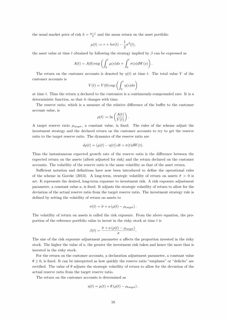
Cui et al. (2011) find similar results: inter-generational risk-sharing through collective, fundedpension plans is welfare-enhancing compared to investing without risk-sharing. Importantly, they

24

find that the anticipated expected welfare gain of a new cohort is not funded by existing or futurecohorts. A collective plan that allows both contributions and benefits to be adjusted in responseto the funding level produces more welfare gains than one which can adjust only contributions oronly benefits.

Cui et al. (2011) point out that the welfare-enhancing aspect of collective pension plans mustbe considered, and not jsut the market values. In their words (Cui et al., 2011, page 3),

The market valuation of [inter-generational risk-sharing] shows that the risk-sharingarrangement is a fair deal when the fund is initially 100% funded. In other words,the market value of funding surplus equals the market value of the deficits in thegenerational account of the entry cohort. However, the schemes with [inter-generationalrisk-sharing] are potentially welfare enhancing, and thus a positive-sum game in welfareterms. An agent joining an underfunded collective scheme is not necessarily worse offin welfare terms. It is possible for well-structured pension schemes to absorb fundingdeficits up to 10-20% by a combination of higher contributions and benefit cuts over anumber of years and still enhance the welfare for participants.

In the collective schemes analyzed by Cui et al. (2011), new members pay contributions whichare expected to fund each member’s pension in isolation. This avoids the plan becoming a Ponzischeme. Members contribute for 40 years and receive a benefit for 15 years. Mortality and earlywithdrawals are ignored, as is the distinction between the sponsoring employer and the activemembers. They analyze:

• A standard DB scheme in which only the contributions are adjusted in response to fundingrisks. Thus only the the sponsoring employer and the active members bear the investmentrisk.

• A CDC scheme in which only the benefits-in-payment are adjusted in response to fundingrisks. Thus only the retirees bear the investment risk.

• A CDC scheme in which both the benefits in payment and the contributions are adjustedin response to funding risks. Thus the sponsoring employer, the active members and theretirees bear the investment risk.

• An individual defined contribution (DC) scheme. The active members and the retirees beartheir own investment risk.

For the DB and CDC schemes, the adjustments to the contributions and benefits-in-payment aregiven by mathematical rules. The parameterization of the rules and the optimal investment andbenefit-in-payment strategy are determined for the first cohort, based on maximizing their expecteddiscounted utility of lifetime consumption. The optimal strategies and parameterizations are keptfor the subsequent cohorts, modulo any adjustments made in line with the rules. The individualDC scheme members follow the optimal investment and consumption strategy that maximizes theirown expected discounted utility of consumption.

Cui et al. (2011, Table 1) find that the CDC scheme in which both the benefits in paymentand the contributions can be adjusted is the most welfare-enhancing under a range of investorand market models. Welfare is measured by the certainty equivalent consumption. Either theindividual DC or the standard DB scheme are the next best, depending on the precise model used.The CDC scheme in which only the benefits-in-payment can be adjusted is the worst performingscheme.

25

Astrup Jensen and Nielsen (2016) consider how worse off is an investor if they invest collectivelycompared to investing on their own. They consider the double impact of being forced to followa suboptimal investment strategy – namely, the collective’s investment strategy rather than theirown, individually optimal investment strategy – and different terminal return-sharing mechanisms.

Specifically, they suppose that the members of a collective receive a share of the investment pro-ceeds that is proportional to their initial contribution. This may be sub-optimal for the individualsince they have different aversion to risk, as measured by different parameterizations of constantrelative risk aversion utility functions.

Although their paper does not directly consider risk-sharing mechanisms, their results are worthyof consideration. Potentially, some members of a collective risk-sharing scheme could be betteroff investing individually. For example, suppose a risk-averse member does not contribute muchinitially relative to the majority of risk-seeking investors. Further assuming that the collectiveinvestment strategy is heavily weighted towards the optimal investment strategy of the risk-seekers,then the risk-averse investor may be – for a utility perspective – far from their optimal, individualstrategy.

For a CDC plan with conditional indexation, similar to some Dutch CDC plans, Kleinow andSchumacher (2017) show that financial fairness is possible for each new cohort. They allow for asponsoring employer as one of the plan’s stakeholders. When the nominal funding ratio is low, i.e.the ratio of the assets to the value of the nominal benefits (excluding pension increases), the faircontributions paid by the new cohort are less than when the nominal funding ratio is high. Thisis because indexation is less likely when the nominal funding ratio is low. However, even when thecontributions from new cohorts are lower, the existing cohorts still benefit from risk-sharing.

Hoevenaars and Ponds (2008) value inter-generational wealth transfers as option prices in variousDB and CDC pension plans. Their focus is on the impact of strategic or structural changes in theschemes. For example switching to a more risky investment strategy results in a loss of value forolder members and a gain for younger members. A switch between a pension scheme targetingflexible contributions and fixed benefits to a scheme aiming for fixed contributions and flexiblebenefits. The latter switch involves a transfer of value from the older members of the schemeto the younger members. Chen et al. (2017) ask when members would leave a CDC scheme, ifparticipation if voluntary. They use option pricing techniques to answer their question. Theyfind that young members are more likely to stay in the scheme than older members; the value ofthe former’s ‘exit option’ is high due to the long time over which it may be exercised. However,assuming that each member has the same contribution rate regardless of their age, the value of eachyear’s pension accrual is much higher for older members than younger ones. This is an incentivefor older members to stay in the scheme.

Donnelly (2017) adjusts the mechanism of Goecke (2013) to a pension plan setting, where mem-bers can leave and join, and benefits are paid out from the plan’s assets. It is assumed thatcontribution rates are fixed.

She finds that the pension scheme – which is a type of CDC plan – reduces the volatility ofbenefits paid out to members, compared to a benchmark Defined Contribution plan. However,members must be prepared to accept reductions in their benefits as a consequence of the lack of asponsor; the asset-to-liability funding ratio is improved by benefit reductions and changes to theinvestment strategy rather than by additional contributions.

26

5 Theoretical risk-sharing frameworksInter-temporal risk-sharing is used to compensate for markets being incomplete. The incomplete-ness referred to in this context arises from the inability of individuals to be exposed to returnsand risks outside of their own lifespan. By inter-temporal risk-sharing through a buffer or similarmechanism, a new generation of customers purchasing a contract are exposed to risks that occurredbefore they bought their contract. This addresses part of the incompleteness but not all of it; oldgenerations whose contract has matured or who have died are not exposed to risks and returnswhich occur after their exit.

5.1 Financial fairness and Pareto-efficiency

A number of recent papers have targeted the question of operating a risk-sharing scheme in afinancially fair and Pareto-efficient way. In these papers, a risk-sharing scheme is defined througha combination of a collective investment decision and a rule for the allocation of investment returnsto the participants of the scheme.

Financial fairness means that the expected value of what an individual gets back from a contractshould be equal to what they put in. Pareto-efficiency looks at the utility of all the scheme’s mem-bers together. A group of contracts are Pareto-efficient if no individual’s utility can be improvedwithout reducing the utility of another individual in the scheme. One of the earliest papers toapply these two conditions in a one-period setting is Gale and Sobel (1979)2.

The authors on this topic must devote a lot of effort to show that a solution exists and, if possible,that the solution is unique. Rarely are they able to find an explicit solution for a particular example.Sometimes they can only characterize a solution and sometimes they can find an iterative algorithmto calculate the solution.

The conclusions of these papers differ when it comes to the solution of their stated problem. Thisis because the problems are different. Some consider only one time-period. Others are multi-periodset-ups, allowing agents to contribute to and receive payments from the risk-sharing scheme. Atwhat times do agents contribute to the scheme? When do agents receive payments out from thescheme? Are investment returns allowed for in the framework? The answers to these questions aredifferent in the models considered in the literature.

5.1.1 One-period model

Here the risk-sharing schemes of Pazdera et al. (2016) and Xia (2004) are presented. Both of themare defined in a one-period model. Thereofre, there is no need for a buffer: money is paid in attime 0 and it is all paid out at time 1.

Pazdera et al. (2016)

Pazdera et al. (2016) consider a group of n agents who wish to divide up the proceeds of acollective investment. The value of the collective investment at the end of the period are modelledby a random variable X. The rules for the division are decided in advance by applying financialfairness and Pareto-efficiency.

The collective investment and the allocation rule are together considered a risk-sharing scheme.A risk-sharing scheme defines a contingent claim payable to the ith agent as a function yi : (0,∞)→

2An earlier, now declassified, version by Gale can currently be found online at http://www.dtic.mil/dtic/tr/fulltext/u2/a047596.pdf.

27

(0,∞) of the end-period investment payoff, for each agent i = 1, . . . , n. In other words, agent 1receives y1(X) at time 1, agent 2 receives y2(X) at time 1, and so on. To ensure that no moreand no less than the investment proceeds are allocated to the agents, the functions must satisfy∑ni=1 yi(x) = x for all x > 0. Similarly, the collective investment proceeds must be positive, i.e.

X ≥ 0 .The agents contribute money to the scheme at the starting time, with the ith agent contributing

a constant amount wi > 0. Although agents assign the same probabilities to random events, theycan have different utility functions.

To define financial fairness, suppose that the expected value of the collective investment Xunder a risk-neutral measure Q equals the sum of the initial contributions, i.e. EQ(X) =

∑ni=1 wi.

Pazdera et al. (2016, Definition 2.1) define an allocation rule (y1, . . . , yn) to be financially fair ifthe expected value of what each agent receives from the collective investment proceeds equals theagent’s initial contribution, i.e. EQ(yi(X)) = wi for i = 1, . . . , n.

To define Pareto-efficiency, some notation is required. For a fixed integer M ≥ 1 and two vectorsa = (a1, a2, . . . , aM ) and b = (b1, b2, . . . , bM ), write a b if am ≥ bm for every m ∈ {1, . . . ,M}and there exists at least one m ∈ {1, . . . ,M} such that am > bm.

A collective risk X and an allocation rule yyy = (y1, . . . , yn) are together Pareto-efficient if theredoes not exist another collective investment proceeds X and allocation rule yyy = (y1, . . . , yn) suchthat (

EP(u1(y1(X)

)), . . . ,EP

(un(yn(X)

))) (EP (u1 (y1(X))) , . . . ,EP (un (yn(X)))) .

Pazdera et al. (2016, Theorem 3.4) are able to establish the existence and uniqueness of a Paretoefficient, financially fair risk-sharing scheme, as represented by the pair consisting of a collectiverisk X and an allocation rule yyy = (y1, . . . , yn). Importantly, they provide an iterative algorithm tocompute the risk-sharing scheme. Their examples are relatively abstract.

Xia (2004)

Xia (2004) considers a similar setting to Pazdera et al. (2016). A group of n agents wish to pooltheir money together to make a collective investment. The payoff of the investment is then dividedamong the agents. There are traded assets available for investment in the market.

Agent i has initial wealth wi > 0 and a utility function Ui. Agent i wishes to maximize theexpected utility of terminal wealth by choosing a suitable investment strategy. Assuming that theoptimal strategy exists, then the expected utility of terminal wealth is represented by ui(wi).

Now suppose that Agent i joins instead the risk-sharing group, for some i ∈ {1, . . . , n}. Theypay initially wi and receive a random payoff ξi ≥ 0 a.s. at the terminal time. In other words, theagent does not follow their own, individually optimal investment strategy. For Agent i to be atleast as well off with risk-sharing,

E (Ui (ξi)) ≥ ui(wi).

For the group of n agents to benefit from risk-sharing, the above inequality should be strict for atleast one agent. In other words, a Pareto-efficient solution is sought. Xia (2004) characterizes thesolution. However, as no explicit solutions are calculated as examples, it is difficult to see how toapply the characterization to a practically-orientated situation.

5.1.2 Multi-period model

Bao et al. (2017)

Bao et al. (2017) propose a framework for risk-sharing within a multi-period model. There are a

28

finite number of agents in the discrete-time model, and the risk-sharing finishes at a finite time.All cashflows occur at fixed times. The set-up is quite different to that of Pazdera et al. (2016).

The agents wish to share their risks, which are cashflows paid to the agents. The risks aremodelled by random variables which represent cashflows received by the system at the fixed times.There is a buffer which is used to spread the risks over the time horizon, through the payment ofcontingent claim to the agents at fixed times. Furthermore, returns are earned on the buffer. Thetotal value of the buffer and the agents’ cashflows received (the risks) is the money to be sharedamong the agents and the buffer.

The total contingent claims paid to the agents at each integer time and the value of the bufferat the terminal time are the decision variables. The random variable Bn represents the size of thebuffer at the nth time point and the random variable Pn is the total contingent claim paid out atthe nth time point as a consequence of the risk-sharing, for n = 1, . . . , N .

It is not required that the financial market is complete. Instead the agents simply have to agreeon a real-world probability measure P and a risk-neutral measure Q.

Exogenous elements of the system are investment returns on the buffer and the risks broughtinto the system by the agents. The random variable Xn represents the risk from the (n − 1)thto the nth time point (money paid into the system), and the random variable Rn is the randomaccumulation factor of the buffer from the (n− 1)th to the nth time point, for n = 1, . . . , N . Thepair (Xn, Rn) is independent of the pair (Xm, Rm), for n ≥ m, but the random variables Xn andRn can be dependent with known joint distribution, for n = 1, . . . , N . The information availableat the nth time point is the filtration Fn = σ{(X1, R1), . . . , (Xn, Rn)}, for n = 1, . . . , N .

For the system to be in balance, it must hold that at the nth time point that the buffer sizeequals the (n− 1)th buffer size increased by the accumulation factor Rn plus the risk Xn paid intothe system less the total contingent claim Pn paid out to the agents, i.e.

Bn + Pn = Xn +Bn−1Rn, for n = 1, 2, . . . , N.

A risk-sharing rule is a random vector (P1, P2, . . . , Pn, Bn) that satisfies the above constraint andsome technical conditions.

To impose the Pareto-efficiency condition, a utility function un is used to evaluate the worthof the contingent claim Pn paid at the nth time point, for each n. A potentially different utilityfunction up evaluates the worth of the final buffer size Bn.

According to Bao et al. (2017, Definition 3.1), a risk-sharing rule (P1, P2, . . . , Pn, Bn) is calledPareto-efficient if there does not exist another risk-sharing rule (P1, P2, . . . , PN , BN ) such that(

EP(u1(P1)),EP

(u2(P2)), . . . ,EP

(uN(PN)),EP

(up(BN)))

(EP (u1 (P1)) ,EP (u2 (P2)) , . . . ,EP (uN (Pn)) ,EP (up (Bn))) .

Furthermore, Bao et al. (2017, Theorem 3.2) show that for a Pareto-efficient risk-sharing rule,there exists positive constants θ1, . . . , θN , θp such that the rule maximizes the function

EP

(N∑n=1

θnun (Pn) + θpup (Bn))

over all possible risk-sharing rules. For any vector of positive constants θθθ = (θ1, . . . , θN , θp),they determine an explicit expression for the Pareto-efficient risk-sharing rule that corresponds toθθθ. There are infinitely many Pareto-efficient risk-sharing rules for {(Xn, Rn)}Nn=1. However, byrequiring financial fairness, the set can be reduced to a single risk-sharing rule.

Under financial fairness, the expected value of the payments to the agents at the nth time pointis equal to a constant, with a different constant for each time point. For example, the constant

29

could equal the expected value of the agents’ risk at the same time point or it could be set usingsome other method. Similarly, the expected value of the buffer at the last time point is equal to aconstant. Bao et al. (2017, Section 4) define a value profile as a vector of constants, representingthe expected value of the agents’ risk at each time point. The expected values are calculated underthe risk-neutral measure Q. The numerical value of each component may be restricted due totechnical conditions on the utility functions.

Given a value profile ννν = (ν1, ν2, . . . , νN , νp), a risk-sharing rule (P1, P2, . . . , Pn, Bn) is financiallyfair if

νn = EQ (Pn) , for n = 1, 2, . . . , N , and νp = EQ (Bn) ,

where expectations are under the risk-neutral measure Q. No discounting is applied.Bao et al. (2017, Theorem 5.1) prove that, given a value profile, there exists a Pareto-efficient,

financially fair risk-sharing rule which is unique. Furthermore, they have devised an iterativealgorithm to calculate the risk-sharing rule to within a desired error bound. As the authorsexplain, the system decides at each time point on how much to pay out (Pn at the nth time point)and how much to keep until the next time point (i.e. how much to place in the buffer at time n).

To illustrate the result of Bao et al. (2017), one of their numerical examples is outlined next.Suppose within a three-period model that there are three agents. Agent n enters at time n−1 andleaves at time n, for n = 1, 2, 3. At time n, Agent n pays the value of Xn into the system. Therandom variable Xn has the distribution

P [Xn = 0.8] = 0.4, P [Xn = 1.2] = 0.6

Q [Xn = 0.8] = 0.5, Q [Xn = 1.2] = 0.5

and receives the contingent claim Pn from the system. Note that EQ(Xn) = 1 and recall that thespecified risk-neutral measure Q is simply any risk-neutral measure that is agreed upon by theagents. The initial buffer size B0 = 1 and the investment returns are zero, so that Rn = 1 forn = 1, 2, 3. Thus the budget constraint that must be satisfied by a risk-sharing rule is

Bn = Bn−1 +Xn − Pn for n = 1, 2, 3.

The financial fairness constraints are

EQ(Pn) = EQ(Xn) = 1 and EQ(Bn) = B0.

Thus each agent should expect to get back what they put into the system. Similarly, the expectedterminal buffer should equal its initial value, so that – in terms of the expectation – the bufferis unchanged by the risk-sharing cashflows. Without requiring Pareto efficiency, it is clear thatsetting Xn := Pn for n = 1, 2, 3 would satisfy the financial fairness constraints.

Imposing Pareto-efficiency, in addition to financial fairness, results in the system developmentas shown in Figure 9. Each path in the tree represents a possible future state of the world, withinthe chosen multi-period model. The utility functions are un(x) := − 1

2x−2 for n = 1, 2, 3 (and

presumably also up(x) := − 12x−2, although the buffer’s utility function does not appear to be

defined in Bao et al. 2017, Section 7.1).Statistics on the mean and standard deviation of the contingent claim payments Pn made to

each agent is shown in Table 1. These are compared to the same statistics of the risks Xn whicheach agent would receive if they weren’t in the risk-sharing system. The statistics are calculatedunder the real-world measure P.

Under the risk-sharing system, the first two agents have the expected payments which are lowerthat what they would get without the system. The variability of the payment size is also lowered

30

B0 = 1

X1 = 0.8P1 = 0.9493B1 = 0.8507

X2 = 0.8P2 = 0.8801B2 = 0.7706

X3 = 0.8P3 = 0.7844B3 = 0.7862

X3 = 1.2P3 = 0.9844B3 = 0.9862

X2 = 1.2P2 = 1.0181B2 = 1.0326

X3 = 0.8P3 = 0.9167B3 = 0.9159

X3 = 1.2P3 = 1.1167B3 = 1.1159

X1 = 1.2P1 = 1.0507B1 = 1.1493

X2 = 0.8P2 = 0.9818B2 = 0.9675

X3 = 0.8P3 = 0.8832B3 = 0.8843

X3 = 1.2P3 = 1.0832B3 = 1.0843

X2 = 1.2P2 = 1.1197B2 = 1.2296

X3 = 0.8P3 = 1.0157B3 = 1.0139

X3 = 1.2P3 = 1.2157B3 = 1.2139

Figure 9: The Open-Ended Buffer example in Bao et al. (2017, Section 7.1). The values of Xn arethe payments into the system from the agents, the values Pn are the payments out ofthe system to the agents and the values Bn represent the size of the buffer, which staysin the system. Investment returns are zero and the agents have a power utility function.The Pareto efficient, financially fair risk-sharing rule is (P1, P2, P3, B3). The values of B3

are close to, but not exactly the same as, those shown in Bao et al. (2017, Table E.6).Here the intermediate and final buffer values are calculated from the budget equationsBn = Bn−1 + Xn − Pn. Otherwise, the values are copied from Bao et al. (2017, TablesE.3-E.5).

by risk-sharing. The risk-sharing system reduces the volatility of payments for the agents and theprice of this is a lower expected return, in absolute terms.

However, in relative terms, all of the agents get a higher expected return per unit of volatility ofpayment size. For example, for the contingent claim paid out at time 1, we have EP (P1) /sdP (P1) =20.335, compared to the same statistic for the payment into the system at time 1 (which is whatthe first agent would get if they didn’t join the risk-sharing system): EP (X1) /sdP (X1) = 5.307.

The last agent has a higher expected payment with the risk-sharing system than without it.However, they have a lower volatility of payment size. The last agent takes more risk, somethingthat is seen in other risk-sharing systems: the last generations have the highest expected returnand the highest volatility of return (Donnelly, 2017; Døskeland and Nordahl, 2008).

31

n EP (Pn) sdP (Pn) EP(Pn)sdP(Pn) EP (Xn) sdP (Xn) EP(Xn)

sdP(Xn)

1 1.010140 0.049676 20.335 1.040000 0.195959 5.3072 1.023884 0.083940 12.198 1.040000 0.195959 5.3073 1.043132 0.127110 8.207 1.040000 0.195959 5.307

Table 1: The Open-Ended Buffer example in Bao et al. (2017, Section 7.1). The values of Xn arethe payments into the system from the agents and the values Pn are the payments out ofthe system to the agents. Investment returns are zero and the agents have a power utilityfunction. The Pareto efficient, financially fair risk-sharing rule is (P1, P2, P3, B3). Thevalues of B3 are close to, but not exactly the same as, those shown in Bao et al. (2017,Table E.6). Here the statistics are calculated using the values of Xn and Pn displayedin Figure 9. They differ slightly from the statistics in Bao et al. (2017, Table 1), due torounding error differences.

Barrieu and Scandolo (2008)

Barrieu and Scandolo (2008) wish to determine the optimal risk exchange between exactly twoagents over many time periods. The idea is that the agents will receive random cashflows at times1, 2, . . . , N outside of the system. The agents will pay the cashflows received at time n into therisk-sharing system and, in return, get a cashflow from the system at the same time n. The rulesfor the allocation of the cashflows between the two agents are decided at time 0. Thus the totalcashflows paid into the system at each time n by the two agents is re-distributed between them attime n, according to the rules decided at time 0. No buffer account is needed. Agents’ preferencesare modelled by quite general preference functionals.

Barrieu and Scandolo (2008) extend Pareto-efficiency from the one period to the multi-periodsetting, and determine necessary and sufficient conditions for the Pareto-efficiency of an allocation.

As an illustration of their results, consider Agent A and Agent B over a two-period model(Barrieu and Scandolo, 2008, Section 5.3.1). The two agents have exponential-type utility functionsuk(x) = − exp (−γkx), for x ∈ R, where γk is the coefficient of risk aversion, for k ∈ {A,B}. Sucha utility function implies constant absolute risk aversion. For example, an individual acting underexponential utility would invest a constant amount in a risky stock in order to maximize theexpected value of the utility of their wealth at a fixed point in time.

Suppose that Agent k receives the random amount X1 at time 1 and X2 at time 2. The preferencefunctional of Agent k ∈ {A,B} is defined as

U (X1, X2) = E (uk(X1)) + βkE (uk(X2)) .

The constants βk > 0 can represent a preference for having money sooner rather than later.Suppose that the total amount of money received by both agents at time n is represented by the

random variable Xn, for n = 1, 2. The agents wish to share this money among themselves, so thatAgent A receives XA

n at time n = 1, 2. As all the money received at time n is re-allocated at timen, it follows that Agent B receives XB

n := Xn −XAn at time n = 1, 2.

The result of Barrieu and Scandolo (2008, Section 5.3.1), here slightly paraphrased, is that anallocation ((XA

1 , XB1 ), (XA

2 , XB2 )) is Pareto-efficient if and only if Agent A receives the allocation

XA1 = 1

γA + γB

(γBX1 + ln

(γBγA

)+ ln (λ)

)

32

at time 1 and the allocation

XA2 = 1

γA + γB

(γBX2 + ln

(βAβB

)+ ln

(γBγA

)+ ln (λ)

)at time 2, for a constant λ ∈ R. The constant λ is determined as the solution of

γA exp(−γAXA

1)

= λγB exp(−γBXB

1)

βAγA exp(−γAXA

2)

= λβBγB exp(−γBXB

2).

The above forms of XA1 and XA

2 imply that Agent B receives the allocation

XB1 = X1 −XA

1 = 1γA + γB

(γAX1 + ln

(γAγB

)− ln (λ)

)at time 1 and the allocation

XB2 = X2 −XA

2 = 1γA + γB

(γAX2 + ln

(βBβA

)+ ln

(γAγB

)− ln (λ)

)at time 2.

33

6 ConclusionVarious mechanisms through which risk-sharing takes place have been described. These rangefrom participating policies, to funded pension plans to theoretical frameworks. The risk-sharingmechanism is usually implicit: money is paid into the risk-sharing system, invested and then paidout following pre-determined rules which aren’t explicitly fair to each generation. The theoreticalframeworks which apply financial fairness and Pareto-efficiency are a notable exception.

In participating policies (Section 3) the risk-sharing is achieved through either a buffer account.The purpose of the buffer may be multi-purpose: in addition to risk-sharing across cohorts of poli-cyholders, it may also smooth returns over a single cohort’s policy duration and provide capital tosupport policy guarantees. Both the insurance company and the policyholders may have legitimateclaims on the buffer. It is difficult to tease out solely the inter-generational risk-sharing aspect inthose participating policies which include it. This is probably why there so few papers written onhe topic.

In funded pension plans (Section 4), the funding ratio may be used as an indirect measure of abuffer. There is no explicit buffer account. Several papers consider the impact of CDC schemes ondifferent generations, usually based on Dutch CDC schemes. The general consensus is that theyare welfare-improving, compared to investing individually. The framework is generally the same:use a simple Black-Scholes market model and assume that equal numbers of generations enter andexit the scheme at the start of each time period.

The theoretical frameworks described in Section 5 come closest to risk-sharing mechanisms whichare designed to be fair. However, it is hard to see how to apply them in practice in a pension savingand spending context. The rules for allocating money are calculated from algorithms, which makethem difficult to communicate. They rely on assigning a utility function to each agent in therisk-sharing system, which immediately makes them quite abstract.

34

ReferencesAstrup Jensen, B. and Nielsen, J. (2016). How Suboptimal Are Linear Sharing Rules? Annals of

Finance, 12(2):221–243.

Bacinello, A. (2001). Fair Pricing of Life Insurance Participating Policies with a Minimum InterestRate Guaranteed. ASTIN Bulletin, 31(02):275–297.

Bao, H., Ponds, E., and Schumacher, J. (2017). Multi-period risk sharing under financial fairness.Insurance: Mathematics and Economics, 72:49–66.

Barrieu, P. and Scandolo, G. (2008). General pareto optimal allocations and applications to multi-period risks. ASTIN Bulletin, 38(1):105–136.

Beetsma, R., Romp, W., and Vos, S. (2012). Voluntary participation and intergenerational risksharing in a funded pension system. European Economic Review, 56(6):1310–1324.

Bennett, P. and Van Meerten, H. (2018). Apples and oranges: a comparison of the key featuresof the legislative and regulatory framework for UK and Dutch defined benefit pension schemes(including Dutch CDC Schemes). Technical report, Pensions Institute, Cass Business School,City University London. Number PI-1803.

Chen, D., Beetsma, R., Broeders, D., and Pelsser, A. (2017). Sustainability of participation in col-lective pension schemes: An option pricing approach. Insurance: Mathematics and Economics,74:182–196.

Cui, J., De Jong, F., and Ponds, E. (2011). Intergenerational risk sharing within funded pensionschemes. Journal of Pension Economics and Finance, 10(1):1–29.

Donnelly, C. (2017). A discussion of a risk-sharing pension plan. Risks, 5(1):1–20. Article number12.

Døskeland, T. and Nordahl, H. (2008). Intergenerational effects of guaranteed pension contracts.The Geneva Risk and Insurance Review, 33(1):19–46.

Gale, D. and Sobel, J. (1979). Fair division of a random harvest: the finite case. In Green, J. R.and Scheinkman, J. A., editors, General Equilibrium, Growth, and Trade: Essays in Honor ofLionel McKenzie, pages 193–198. Academic Press, New York, USA.

Goecke, O. (2013). Pension saving schemes with return smoothing mechanism. Insurance: Math-ematics and Economics, 53(3):678–689.

Gollier, C. (2008). Intergenerational risk-sharing and risk-taking of a pension fund. Journal ofPublic Economics, 92(5):1463–1485.

Grosen, A. and Jorgensen, P. (2000). Fair valuation of life insurance liabilities: The impact ofinterest rate guarantees, surrender options, and bonus policies. Insurance: Mathematics andEconomics, 26(1):37–57.

Grosen, A. and Jorgensen, P. (2002). Life insurance liabilities at market value: An analysis ofinsolvency risk, bonus policy, and regulatory intervention rules in a barrier option framework.Journal of Risk and Insurance, 69(1):63–91.

35

Guillen, M., Jørgensen, P., and Nielsen, J. (2006). Return smoothing mechanisms in life andpension insurance: Path-dependent contingent claims. Insurance: Mathematics and Economics,38(2):229–252.

Haberman, S., Ballotta, L., and Wang, N. (2003). Modelling and Valuation of Guarantees inWith-Profit and Unitised With Profit Life Insurance Contracts. Technical report, Cass BusinessSchool, London. Working Paper Actuarial Research Paper No 146.

Hansen, M. and Miltersen, K. (2002). Minimum rate of return guarantees: The danish case.Scandinavian Actuarial Journal, 2002(4):280–318.

Hoevenaars, R. and Ponds, E. (2008). Valuation of intergenerational transfers in funded collectivepension schemes. Insurance: Mathematics and Economics, 42(2):578–593.

Kleinow, T. and Schumacher, J. (2017). Financial fairness and conditional indexation. Scandina-vian Actuarial Journal, 8:651–669.

Kling, A., Richter, A., and Ruß, J. (2007). The interaction of guarantees, surplus distribution, andasset allocation in with-profit life insurance policies. Insurance: Mathematics and Economics,40(1):164–178.

Miltersen, K. and Persson, S. (2003). Guaranteed investment contracts: Distributed and undis-tributed excess return. Scandinavian Actuarial Journal, 2003(4):257–279.

Orozco-Garcia, C. and Schmeiser, H. (in press). Is Fair Pricing Possible? An Analysis of Partici-pating Life Insurance Portfolios. Journal of Risk and Insurance.

Pazdera, J., Schumacher, J., and Werker, B. (2016). Cooperative investment in incomplete marketsunder financial fairness. Insurance: Mathematics and Economics, 71:394–406.

Xia, J. (2004). Multi-agent investment in incomplete markets. Finance and Stochastics, 8:241–259.

Zemp, A. (2011). Risk comparison of different bonus distribution approaches in participating lifeinsurance. Insurance: Mathematics and Economics, 49(2):249–264.

36