investment in production resource flexibility
TRANSCRIPT
Investment in Production Resource Flexibility: An empirical investigation of methods for planning under uncertainty
Elena Katok † MS&IS Department
Penn State University University Park, PA 16802
William Tarantino Center for Army Analysis
Fort Belvoir, VA [email protected]
Terry P. Harrison
MS&IS Department Penn State University
University Park, PA 16802 [email protected]
7 August 2001
† Corresponding author

-1-
Investment in Production Resource Flexibility: An empirical investigation of methods for planning under uncertainty
Elena Katok, William Tarantino and Terry P. Harrison
We examine several methods for evaluating resource acquisition decisions under uncertainty. Traditional methods may underestimate equipment benefit when part of this benefit comes from decision flexibility. We develop a new, practical method for resource planning under uncertainty, and show that this approach is more accurate than several commonly used methods. We successfully applied our approach to an investment problem faced by a major firm in the aviation information industry. Our recommendations were accepted and resulted in estimated annual savings in excess of $1 million (US).
Keywords: manufacturing flexibility, stochastic programming, and sampling
In recent years, many firms have found it increasingly important to invest substantially in
technology to maintain a competitive edge. Technological improvements often require superior
production methods, and some firms find themselves constantly evaluating opportunities for
investments in new production resources. These decisions can easily become crucial to survival in
a competitive market place. While essential to the well being of firms, production investment
decisions are extremely difficult because they involve planning under uncertainty. For example,
when a new production resource provides manufacturing flexibility, the benefit of this flexibility
can be easily underestimated. As Jordan and Graves [16] point out: “in capacity and flexibility
planning, investment costs for flexible operations are typically quantified; however, it is less
common to quantify the benefits because demand uncertainty is not explicitly considered by the
planners. Since flexibility is expensive, this typically results in decisions not to invest in it.”
The benefits of a new production resource can emerge in three ways:
1. Lower cost due to superior performance
2. Increased capacity
3. Increased decision flexibility.

-2-
The first two sources of benefit are fairly intuitive: cost savings may result if a new resource
provides a more efficient production process or introduces a new dedicated process. If a new
resource is added to the current production system at a particular stage, capacity at that stage may
increase. If that stage previously formed a bottleneck, the throughput of the entire system increases
(Goldratt and Cox [12]), potentially yielding cost savings. The third source of benefit comes from
increased decision flexibility (Benjaafar et al. [2]). Decision flexibility is the ability to postpone
decisions until more information is obtained. When a new production resource is added to the
current system, it can increase decision flexibility by either providing additional capacity where it is
needed, or by providing an additional routing for a part. To correctly estimate the impact of a
flexible resource, a model must include all three sources of benefit.
With this study we contribute to manufacturing flexibility planning research in three ways:
• We describe a new and better method that accurately accounts for all three sources
of flexibility benefit, and that is practical enough to be used for large and complex
real-world problems.
• We implement and use the new method to help with a real flexibility-planning
decision faced by Jeppesen Sanderson, Inc. (Jeppesen), a manufacturing company,
and generate annual savings in excess of $1 million.
• We clearly demonstrate, using the Jeppesen investment problem as a case study, how
other commonly used methods can consistently under-estimate the benefit of
flexibility.
This paper is organized as follows. First, we describe the problem and summarize relevant
literature in Section 1. In Section 2, we develop a formal mathematical model for flexibility
planning and show analytically that some commonly used methods generally under-value
flexibility. We also describe our new sampling-based optimization algorithm that assesses the
benefit of manufacturing flexibility more accurately than existing methods. In Section 3, we
-3-
describe the flexibility-planning problem faced by Jeppesen and the application of our method to
this problem. In Section 4 we demonstrate that alternative methods significantly under-estimate the
benefit of flexibility at Jeppesen. We discuss the impact of our work at Jeppesen in Section 5 and
summarize this work’s contributions in Section 6.
1. Problem Description
Flexibility planning has been studied extensively during the last decade, and here we do not
attempt to provide an exhaustive survey. For a summary of flexibility categories and measures see
Sethi and Sethi [21] or Gupta and Goyal [14]. Recent frameworks for flexibility planning span the
spectrum from qualitative and descriptive (Gerwin [11]), to purely theoretical (deGroote [8], van
Mieghem [28]), to empirical (Suarez et al. [25]), to managerial (Upton [27]).
Our view is that the problem of evaluating an investment in a new production resource in
general, and in a flexible resource in particular, consists of two parts. The first part is how to
accurately estimate the future benefits the new resource will generate (for example an uncertain
stream of cash flows). The second question is how to properly determine the value of these
benefits. In this paper, we focus on the first part: properly estimating the future benefits attributed
to an investment. A large decision analysis and real options pricing1 literature already addresses the
second question. Smith and Nau [24] show the circumstances under which the real options and the
decision analysis approaches are consistent.
Consider a problem setting where a manufacturing firm has an opportunity to improve its
production process by purchasing a new piece of equipment. While the cost of the new resource is
1 The idea behind the real option pricing approach is to apply finance methods for valuing put and call options to “real” projects. If one can construct a portfolio of financial instruments that exactly replicates the real project’s cash flows in every possible state of the world, the market value of this portfolio is the same as the value of the real project. See Smith and McCardle [23] for a detailed summary of real option pricing approach.

-4-
known, its real benefit is not. To find the true benefit of the new resource, we need to be able to
compare the performance of the resulting production system with and without the new resource.
We have two ways to do this comparison. We can try to model the systems either as it is
actually used or as it should be used. The first method can be achieved with a simulation model,
and the second with an optimization model (for example, stochastic programming). Examples of
the pure simulation approach include Azzone and Bertele [1], Suresh [26] and Das and
Nagendra [7]. Simulation models are conceptually easy to understand and implement, but they can
lead to sub-optimal results. Ramasesh and Jayakumar [20] take simulation one step further, by
using it to generate realizations of uncertain parameters that are then used as data in an optimization
model. We will say more about the Ramasesh and Jayakumar approach in Section 2.2.
Alternatively, optimization methods such as stochastic programming in theory yield optimal
solutions, but real-sized, multi-stage stochastic programming models with recourse are often
intractable. Examples of approaches based on stochastic programming include Sinha and Wei [22],
Gupta, Gerchak and Buzacott [13] and Fine and Freund [10]. Recently much work has been done
on developing approximation methods for certain classes of stochastic programming problems (see
Birge and Louveaux [3] and Infanger [15]).
Successful applications of stochastic programming include the work of Eppen, Martin and
Schrage [9] who developed a model for General Motors that uses a scenario approach to select the
type and level of production capacity. Mulvey, Gould and Morgan [19] describe an asset-and-
liability management system developed for Towers Perrin-Tillinghast that uses stochastic
programming to help its clients make major business decisions. Carino et al. [6] describe another
asset and liability management system developed for Frank Russell Company and The Yasuda Fire
and Marine Insurance Co., Ltd., to determine the optimal investment strategy.

-5-
The new method we describe here is an extension of the approach first described by Katok [17].
It combines optimization with sampling to approximate system performance under uncertainty.
The dynamics of the algorithm are consistent with decision-making practices shown to be superior
by Benjaafar et al. [2]. The new method is more intuitive and is easier to implement than stochastic
programming, and is more robust and general than pure simulation.
2. Model Development
To determine the benefit of investing in a new production resource, we wish to estimate the
additional cash flows that the new resource will generate. To accomplish this we model the current
system (without the new resource) to determine the base cash flows. We then model the system
with the new resource to determine the cash flows from the enhanced system. The difference
between the two sets of cash flows can be attributed to the new resource. If the value of these
additional cash flows (determined via decision analysis or real option pricing) exceeds the cost of
the new resource, the new resource is worth obtaining.
Theoretically, the proper way to determine the performance of a system under uncertainty is
with a multi-stage stochastic programming. The objective function value of this model represents
the system’s performance. Since such large problems are notoriously difficult to solve to
optimality, we develop approximate solutions. In the following sections we develop the stochastic
programming formulation (also called the recourse problem) of the resource acquisition decision.
2.1 Problem Formulation
We use the stochastic programming notation of Birge and Louveaux [3], where random
variables are denoted in bold. Consider a manufacturing firm that produces a set of products
{ }|1,p P=P � using a general assembly process. Each p ∈P represents either a finished product
or a sub-assembly. We can specify any type of bill of materials (BOM) structure by defining a set

-6-
pS (successors of p) for each product p to include immediate successors of p in the BOM. We also
let ,p jk be the number of units of p required to make one unit of j when pj ∈S . If p is an end-item,
p = ∅S . Let ΡΡΡΡ be the set of production resources. Since each p ∈P represents a product at a
particular production stage, we assume without loss of generality, that it needs to be processed only
by one resource at each stage, although there may be alternative ways to process a product at a
stage. Finally, let us assume that the model can be naturally decomposed into convenient time
blocks { }| 1, Jτ τ= =J l , in such a way that there are not “many” interactions among the time
blocks (ideally no interactions at all). Specifically, we assume that inventory cannot be carried
across time blocks. We also assume that backorders across time blocks are allowed, but the
interpretation of a backorder during the last period of a time block changes to unmet demand, so
there is never any backorder that has to be met in the first period of a time block. Each time block
τ ∈ J , in turn consists of time periods t τ∈ T . Therefore, the model can be decomposed into
separate multistage stochastic programs for each time block τ. We identify each period in the
model by a pair of indexes, ( ),t τ , representing the time period t of the time block τ. We introduce
the time block notation for convenience, and without loss of generality. If time horizon cannot be
broken into time blocks, we simply have a single time block in the problem. Since the Ramasesh
and Jayakumar [20] model requires the use of time blocks, we introduce them here, to ensure
consistency among models.
Let ,tpτd be the demand for the end items only (in period t of time block τ for product p) and
a random variable. When p is an intermediate item, , 0tpτ =d . If demand in period t is not filled, a
unit backorder cost ,tp
τλ is charged for the period. The processing time for product p on resource r
-7-
at time t of time block τ is ,,
tp ra τ , and we assume that processing times do not span multiple periods.
If a product does not need to be processed on a particular resource then ,, 0 ,t
p ra tτ τ= ∀ . Different
resources involve different operating requirements, so let rw be the cost of one unit of time on
resource r. Finally, each resource has ,trc τ units of capacity available at time t of time block τ.
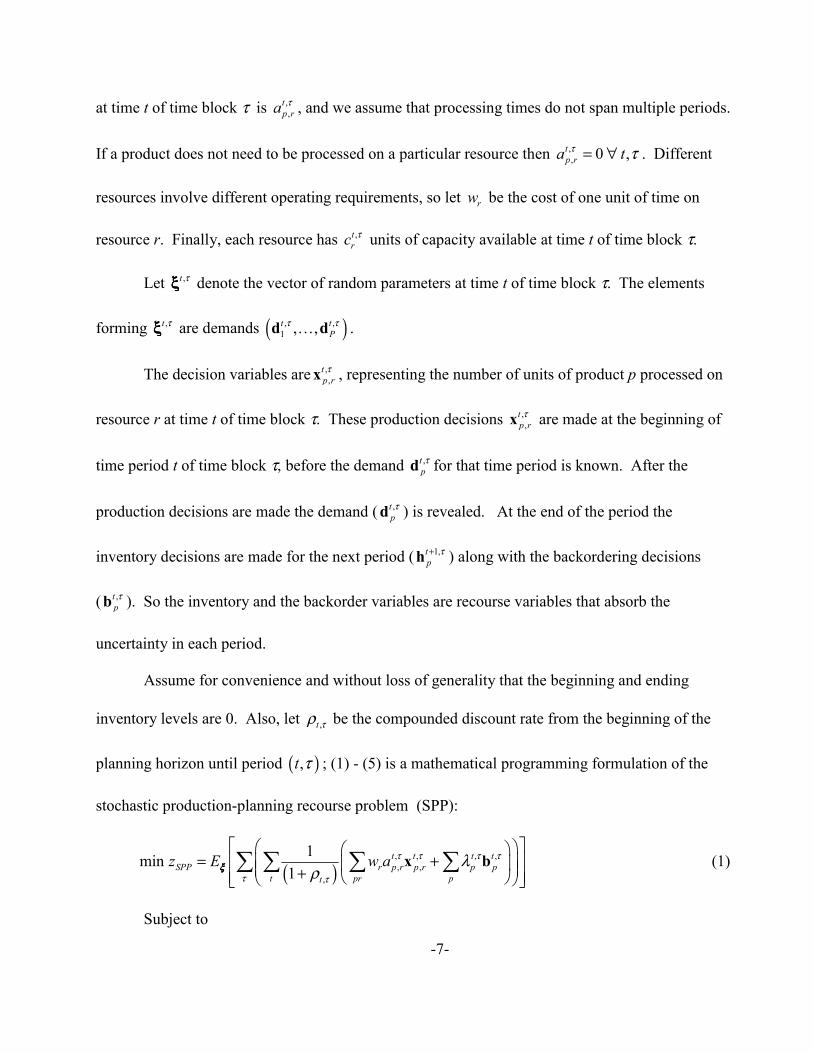
Let ,t τξξξξ denote the vector of random parameters at time t of time block τ. The elements
forming ,t τξξξξ are demands ( ), ,1 , ,t t
Pτ τd dl .
The decision variables are ,,
tp rτx , representing the number of units of product p processed on
resource r at time t of time block τ. These production decisions ,,
tp rτx are made at the beginning of
time period t of time block τ, before the demand ,tpτd for that time period is known. After the
production decisions are made the demand ( ,tpτd ) is revealed. At the end of the period the
inventory decisions are made for the next period ( 1,tp
τ+h ) along with the backordering decisions
( ,tpτb ). So the inventory and the backorder variables are recourse variables that absorb the
uncertainty in each period.
Assume for convenience and without loss of generality that the beginning and ending
inventory levels are 0. Also, let ,t τρ be the compounded discount rate from the beginning of the
planning horizon until period ( ),t τ ; (1) - (5) is a mathematical programming formulation of the
stochastic production-planning recourse problem (SPP):
( ), , , ,, ,
,
1min1
t t t tSPP r p r p r p p
t pr pt
z E w a τ τ τ τ
τ τ
λρ
= + +
∑ ∑ ∑ ∑x bξξξξ (1)
Subject to

-8-
, , , , , 1, 1,, , ,
,
0 , 1,p
t t t t t t tp p r p j j r p p p p
r r jk p tτ τ τ τ τ τ τ τ− +
∈
+ − − + − − = ∀ ≠∑ ∑S
h x x d b b h (2)
1, 1, 1, 1, 1, 2,, , ,
,
0 ,p
p p r p j j r p p pr r j
k pτ τ τ τ τ τ τ∈
+ − − + − = ∀∑ ∑S
h x x d b h (3)
, , ,, , , ,t t t
p r p r rp
a c r tτ τ τ τ≤ ∀∑ x (4)
, , ,,, , 0 , , ,t t t
p p r p p r tτ τ τ τ≥ ∀h x b (5)
Equation (1) is the objective function that minimizes the total expected discounted
production and backorder cost, with expectation taken with respect to the random vector ξξξξ.... If the
planning horizon is sufficiently long, we should include the inventory holding costs as well.
Equations (2) and (3) are the set of material balance constraints that ensures that no product is
processed until all its predecessors are available. Note that equation (3) is for the first period of a
time block, where backorder from the previous time block does not have to be met. Equation (4) is
the set of capacity constraints.
In practice, more simplistic procedures than stochastic programming are used to determine
the value of flexibility, and we review two such procedures in the next section. Sometimes simple
simulation-based methods do an adequate job, correctly approximating the benefit of flexible
resources; nevertheless, at times, as we will demonstrate, simplistic methods may systematically
underestimate the benefit of flexible equipment.
2.2 Alternative Methods
2.2.1 The “Wait and See” Model
If uncertainty can be approximated by a set of scenarios, then one way to determine the
value of flexibility is to solve the so-called “wait and see” problem (WS). If we let the individual

-9-
scenarios correspond to realizations of the random variable ξξξξ, then equations (6) - (10) can define
the optimization problem associated with one particular scenario ξξξξ.
( ) ( ), , , ,
,
1min1
t t t tr pr pr p p
t pr pt
z w a x bτ τ τ τ
τ τ
λρ
= + + ∑∑ ∑ ∑ξξξξ (6)
Subject to
, , , , , 1, 1,, , , 0 , 1,
p
t t t t t t tp p r p j j r p p p p
r r, j Sh x k x d b b h p tτ τ τ τ τ τ τ τ− +
∈
+ − − + − − = ∀ ≠∑ ∑ (7)
1, 1, 1, 1, 1, 2,, , , 0 ,
p
p p r p j j r p p pr r, j S
h x k x d b h pτ τ τ τ τ τ τ∈
+ − − + − = ∀∑ ∑ (8)
, , ,, , , ,t t t
p r p r rp
a x c r tτ τ τ τ≤ ∀∑ (9)
, , ,, 0 , , ,t t t
p p r ph ,x ,b p r tτ τ τ τ≥ ∀ (10)
Here all variables and parameters indexed by t and τ represent quantities in period t of time-block τ.
Denote an optimal solution to (6) - (10) as ( )*x ξξξξ (since the x variables uniquely determine
the h and the b variables), and the corresponding objective function value as ( )z ξξξξ . We can then
compute ( )WSz E z= ξξξξ ξξξξ , as the expected value of objective function values of deterministic sub-
problems corresponding to realizations of the random variables in all scenarios. This solution is
known in the literature as the “wait and see” solution (Birge and Louveaux [3]).
Computing ( )WSz E z= ξξξξ ξξξξ exactly is unlikely to be practical because the number of scenarios
can be extremely large. If this is the case, we must approximate ( )WSz E z= ξξξξ ξξξξ with a sample-mean
estimate of WSz . This is the approach we take for the empirical comparisons discussed in Section 4.

-10-
2.2.2 The Aggregate Model
A natural method to simplify computations of the optimal value of the objective function for
the deterministic production planning problem and establish a base line on the benefit of new
equipment is to consider an aggregate formulation (APP). This method is especially convenient
when random variables can be naturally separated into several time blocks, with not many
interactions among the time blocks. This is the Ramasesh and Jayakumar [20] approach. Eppen,
Martin and Schrage [9] use a similar approach, aggregating their capacity planning model
developed for General Motors into five yearly time blocks.
In the aggregate formulation, the planning horizon consists of time blocks,
{ }| 1, Jτ τ= =J � . We aggregate the products into end-items. In this case the set ΠΠΠΠ of products
includes end-items only, and the decision variables ,p rτx represent the number of units of the end-
item p processed on resource r during the time-block τ. We can measure the per unit requirement
of resource r by product p in time block τ , ,, ,
tp r q r
t qA a
τ
τ τ
∈= ∑∑
T where q was in the BOM for p in the
SPP model. The demand for product p is now the aggregate demand for the time block,
tp p
t τ
τ
∈= ∑D d
T. The capacity of resource r is the aggregate capacity for the time block, t
r rt
C cτ
τ
∈= ∑
T. If
capacity is insufficient to fill current time-block demand, the product is backordered, and pτB is the
total backorder of product p for time block τ. Note that the nature of backordering can be different
in APP than in SPP, since in APP backordering represents the unmet demand, while in SPP
backorders can be filled in subsequent periods. If we allow some demand at the end of a time block
to remain unmet in SPP, that unmet demand has the same meaning as pτB in APP. The backorder
cost pλ = ,tp
τλ when t is the last period in a time block τ . Since no inventory is carried across time
-11-
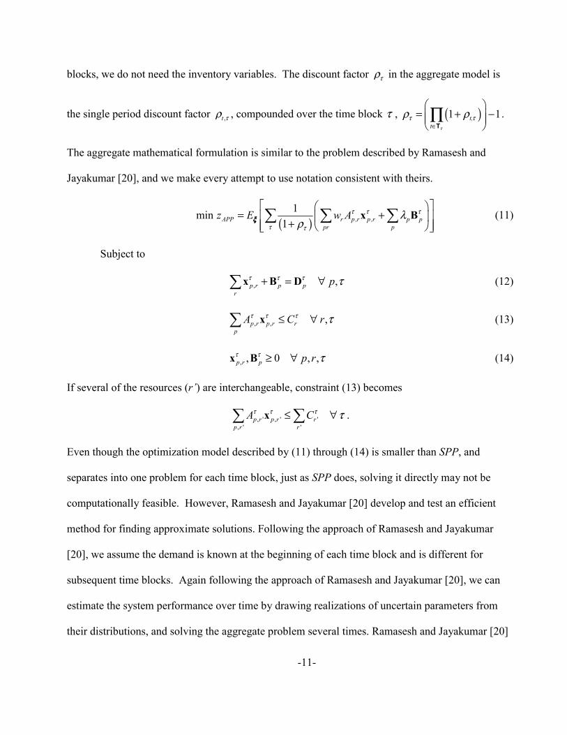
blocks, we do not need the inventory variables. The discount factor τρ in the aggregate model is
the single period discount factor ,t τρ , compounded over the time block τ , ( )1 1t,t τ
τ τρ ρ∈
= + − ∏
T.
The aggregate mathematical formulation is similar to the problem described by Ramasesh and
Jayakumar [20], and we make every attempt to use notation consistent with theirs.
( )
1min1APP r p ,r p ,r p p
pr pz E w Aτ τ τ
τ τ
λρ
= + +
∑ ∑ ∑x Bξξξξ (11)
Subject to
, ,p r p pr
pτ τ τ τ+ = ∀∑x B D (12)
, , ,p r p r rp
A C rτ τ τ τ≤ ∀∑ x (13)
, , 0 , ,p r p p rτ τ τ≥ ∀x B (14)
If several of the resources (r’) are interchangeable, constraint (13) becomes
, ' , ' ', ' '
p r p r rp r r
A Cτ τ τ τ≤ ∀∑ ∑x .
Even though the optimization model described by (11) through (14) is smaller than SPP, and
separates into one problem for each time block, just as SPP does, solving it directly may not be
computationally feasible. However, Ramasesh and Jayakumar [20] develop and test an efficient
method for finding approximate solutions. Following the approach of Ramasesh and Jayakumar
[20], we assume the demand is known at the beginning of each time block and is different for
subsequent time blocks. Again following the approach of Ramasesh and Jayakumar [20], we can
estimate the system performance over time by drawing realizations of uncertain parameters from
their distributions, and solving the aggregate problem several times. Ramasesh and Jayakumar [20]

-12-
show that this approach gives solutions very close to optimal solutions to the aggregate problem.
However, APP is a relaxation of SPP, and therefore zAPP is a lower bound on zSPP.
Now let us analyze APP’s estimates for the benefit of a flexible resource. First, let us say
that we have the base-line system consisting of a set of resources ΡΡΡΡ, and a new system, consisting of
a set of resources 'R , where { }' newr= ∪R R . Let ( ) ( ) ( )' 'APP APP APPV z z= −R R R represent the
APP estimate of the benefit of the new set of production resources{ }newr , and also let
( ) ( ) ( )' 'WS WS WSV z z= −R R R represent the WS estimate of the benefit of{ }newr . Recall that we
postulated that there are three sources of benefit of a resource: (1) lower production cost, (2)
capacity, and (3) decision flexibility. The problem APP considers the cost of operating a resource
(unlike the Ramasesh and Jayakumar [20] formulation that looks at the time rather than the cost), so
the portion of the new resource benefit due to any productivity improvement that results in lower
production cost is addressed by APP.
APP only partially accounts for benefit due to capacity. Problem APP has a capacity
constraint that preserves the aggregate capacity for the time block. It is possible, however, to
observe the aggregate capacity constraint while violating capacity constraints for single periods.
For example, if each day has eight hours of capacity, and the time block has two days, the aggregate
capacity constraint tells us that we cannot exceed the 16 hours capacity in a two-day period. But a
production plan requiring 10 hours on day 1 and 6 hours on day 2 is still aggregate-feasible,
although the plan exceeds day 1 capacity and allows an unrealistic shift of available hours. A
stronger capacity constraint would force the model to allocate hours properly and highlight the
benefits from having the additional capacity on days when it is required. Since APP has a weaker

-13-
capacity constraint than SPP, the benefit of the new resource due to capacity can be underestimated
because the model will not identify benefits on capacitated days.
When decisions are made in APP, all relevant time-block information is known. Benjaafar
et al. [2] show that decision flexibility provides no benefit if no relevant future information is
expected. This result implies that APP does not account for any benefit of the new resource due to
an increase in decision flexibility, but it does provide an approximation for the benefit from
efficiency gain and partial benefit from capacity gain. Similarly, ( ) ( )' 'WS APPV V−R R provides an
estimate for the gains from capacity not captured in ( )'APPV R . And most importantly,
( ) ( )' 'SPP WSV V−R R provides an estimate for the gains from decision flexibility.
2.3 The New Method
Both, APP and WS make a part of the SPP recourse problem into a deterministic problem
and then solve a sequence of deterministic problems with parameters representing realizations of
stochastic parameters. The solution to a problem where stochastic parameters are replaced with
their realizations is called a wait-and-see solution. Birge and Louveaux [3] (p. 140) prove that the
wait-and-see solution is a lower bound on the recourse problem solution (in our terminology,
WS SPPz z≤ ). Birge and Louveaux [3] also describe the notion of the expected result of using the
expected value solution (EEV) (p. 139). This is the expected system performance that results if, at
the beginning of the planning horizon, we solve a problem replacing all stochastic parameters with
their expected values and implement the solution. Birge and Louveaux [3] show that EEV is an
upper bound on the recourse problem solution zSPP, because, by construction, EEV is always a
feasible solution to the recourse problem. It turns out that typically, EEV is a weak upper bound.
Our goal is to develop an algorithm with a stronger upper bound on zSPP.

-14-
We begin by looking at the decision-making process under uncertainty. Benjaafar et al. [2]
postulate that there are two general approaches to “flow control decisions in manufacturing.” The
planning-based approach applies when a production plan is determined prior to the beginning of
production (at t = 0) and is rigidly adhered to. It is similar in flavor to the EEV solution. The real
time based, or opportunistic approach allows decision making to be “contemporaneous with action
implementations.” Decisions are made based on the state of the system, and no decision is
implemented until it has to be. Benjaafar et al. [2] show that “under conditions of uncertainty,
opportunism is superior to planning.”
To generate an upper bound on zSPP we apply the opportunistic decision making process and
use the rolling horizon strategy (see Bitran and Sarkar [4] and Bitran and Yanasse [5]). Under this
strategy, we solve a multi-period problem each period, but only implement first-period decisions
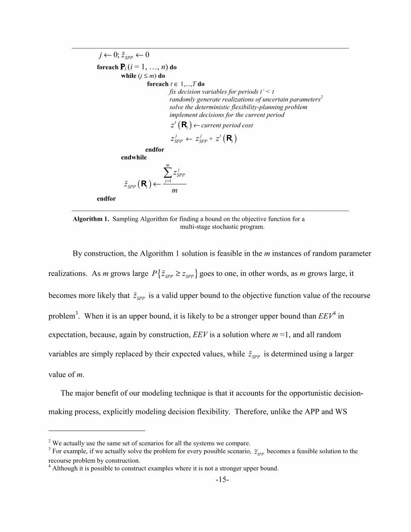
and keep track of the first period performance measures. Algorithm 1 formally outlines the method,
and the resulting process for estimating the performance of a production system under uncertainty.
We wish to estimate the difference in the total expected cost of operation over the T-period
planning horizon of n different systems with different sets of production resources. Let ΡΡΡΡi denote
the set of resources in the ith system under consideration. Let ( )tiz R be the cost during period t of a
system with resources ΡΡΡΡi. We estimate the objective function value of the recourse problem zSPP
with an estimate SPPzC by repeating the opportunistic decision-making task m times.
-15-
0; 0SPPj z← ←�
foreach ΡΡΡΡi (i = 1, …, n) do while (j ≤ m) do foreach t ∈ 1,...,T do
fix decision variables for periods t’ < t randomly generate realizations of uncertain parameters2
solve the deterministic flexibility-planning problem implement decisions for the current period
( )tiz R ← current period cost
jSPPz ← j
SPPz + ( )tiz R
endfor endwhile
( ) 1
mj
SPPj
SPP i
zz
m=←∑
RC
endfor
Algorithm 1. Sampling Algorithm for finding a bound on the objective function for a multi-stage stochastic program.
By construction, the Algorithm 1 solution is feasible in the m instances of random parameter
realizations. As m grows large { }SPP SPPP z z≥� goes to one, in other words, as m grows large, it
becomes more likely that SPPzC is a valid upper bound to the objective function value of the recourse
problem3. When it is an upper bound, it is likely to be a stronger upper bound than EEV4 in
expectation, because, again by construction, EEV is a solution where m =1, and all random
variables are simply replaced by their expected values, while SPPzC is determined using a larger
value of m.
The major benefit of our modeling technique is that it accounts for the opportunistic decision-
making process, explicitly modeling decision flexibility. Therefore, unlike the APP and WS
2 We actually use the same set of scenarios for all the systems we compare. 3 For example, if we actually solve the problem for every possible scenario, ~zSPP becomes a feasible solution to the recourse problem by construction. 4 Although it is possible to construct examples where it is not a stronger upper bound.

-16-
models, our new model will be less likely to under-estimate the benefit of a resource as much as
APP and WS when that resource provides decision flexibility.
3. Jeppesen Sanderson, Inc.
The applied portion of this work focuses on Jeppesen’s production system for flight manual
revision service. For a more complete description of Jeppesen see Katok, Tarantino and Tiedeman
[18]. Airway safety considerations dictate that all pilots on all flights must have a set of airport
maps, enroute charts, and other flight information for the area within a 200-mile radius of the
planned route. Flight information changes constantly, so this material must be updated regularly.
For example, about 75% of all charts are revised at least once annually, and many charts are
amended much more often. Enroute charts that cover large areas change on average four times a
year. A typical Jeppesen chart is shown in Figure 1.
Jeppesen usually configures its flight manuals by geographical area. Many pilots subscribe
to what Jeppesen refers to as the “Airway service;” however, many of Jeppesen’s large customers,
including major airlines such as United, American, and Delta and package delivery services such as
FedEx and UPS request special subscription packages. These special packages, called “Air Carrier
coverages,” can differ from standard coverages because they contain charts with special
information, a customized configuration of pages, or other specific features that a customer might
request. Jeppesen maintains over 200 different standard coverages and over 2,000 different tailored
coverages, made up of over 100,000 distinct images.

-17-
Figure 1. A typical Jeppesen chart
When critical aviation information changes (such as a runway at an airport is closed or
expanded), the change affects multiple Jeppesen charts. Typically, a change affects one airway
chart and several customized air carrier charts. When a chart is revised, Jeppesen issues a new
manual page to all customers subscribing to coverages containing this page within one week of the

-18-
change. Every week Jeppesen sends out between 3 and 25 million pages to over 300,000 different
customers. Some weeks over 1,500 images, affecting over 1,000 different coverages must be
altered. Figure 2 shows a diagram of the Jeppesen revision management and production process.
Aviation information
data
Is this data accurate and important?
STOP No
Imaging and printing
Machine Collating
Final Assembly
Image edited electronically
Shipping
Yes
Figure 2. Revision management and production process at Jeppesen.
When information regarding a possible change first reaches Jeppesen, a decision is made as
to whether this data is important or permanent enough to amend a chart. Some changes do not need
to be included on a chart. For example, a runway closing for 20 minutes on a particular day would
not require a revision (and will be handled with a ‘notam’). If a change to a chart is deemed
necessary, the first step of the process involves electronically editing the image file. Some
alterations are easy to make taking less than 5 minutes, while other changes can require as much as
8 hours of work. After an image file has been edited electronically, a new negative is printed. This
negative goes to the first step of the production process, imaging and printing, where it is stripped
onto a plate containing 21 negatives, the plate is printed, cut into individual sheets, and specially
bound. Sheets then go into the machine collating area, where they are collated into sections. Each
section contains up to 25 sheets that will eventually all go into the same coverage. At this point
large maps, called folds, are not included into sections, because collating machines cannot handle
folded material. Sections and folds go into the final assembly area, where prior to the
implementation of our work they were manually assembled into coverages and stuffed into

-19-
envelopes. Large boxes of envelopes go on to the shipping department. If a coverage completes
final assembly on time it is shipped using standard shipping services, but if it is late the service is
upgraded to overnight delivery.
Figure 3. The manual process
The bottleneck of the production process forms in final assembly, highlighted in Figure 2. Prior to
implementation of our work, in final assembly sections and folds were arranged and stuffed
manually, often by a large number of temporary employees. Figure 3 shows a photograph of a
typical Jeppesen assembly process. The use of temporary employees has several disadvantages for
Jeppesen. They are often unfamiliar with the work, and tend to be less productive and make more
mistakes than full-time employees. Jeppesen customers do not tolerate errors, so all errors are
detected and corrected at great expense prior to shipping. The availability of temperary employees
can also be unpredictable. Because of these problems, Jeppesen management wished to evaluate
the purchase of new, automated technology, called folder collator, for final assembly, and asked us
to help them with this decision. The dynamic and complex nature of the Jeppesen operating

-20-
environment makes properly determining the benefit of the new technology difficult, and hence the
application of our method well-warranted.
4. Empirical Comparisons
In this section we demonstrate how the three approaches to estimating the benefit of a
flexible resource can yield different results. Jeppesen operates on an 8-week revision cycle
involving three week-types with differing demand volumes: odd weeks have relatively low volume,
even weeks have medium volume, and eighth weeks have the highest volume. Over time, revision
characteristics in terms of overall volume (number of customers), the number of different
coverages, average volume, and coverage size in terms of both, folds and flats, have been evolving.
Figures 4a and 4b show historical trends in weekly revision for relevant dimensions since 1995.
Total Quantity: envelop count
0
20,000
40,000
60,000
80,000
100,000
120,000
140,000
1 17 33 49 65 81 97 113 129 145 161
Number of Different Coverages Revising
0
50
100
150
200
250
300
350
1 17 33 49 65 81 97 113 129 145 161

-21-
Average Quantity: customers per coverage
0
200
400
600
800
1,000
1,200
1,400
1,600
1,800
2,000
1 17 33 49 65 81 97 113 129 145 161
Average Number of Flats per Coverage
0
10
20
30
40
50
60
70
80
90
1 17 33 49 65 81 97 113 129 145 161
Average Number of Folds per Coverage
0
1
2
3
4
5
6
7
8
1 17 33 49 65 81 97 113 129 145 161
Figure 4a. Revision characteristics over time: Airway. The number of airway coverages revising increases significantly over time, while the average number of Airway customers per coverage declines, highlighting the fact that demand for customized products increases over time.

-22-
Total Quantity: envelop count
020,00040,00060,00080,000
100,000120,000140,000160,000180,000200,000
1 17 33 49 65 81 97 113 129 145 161
Number of Different Coverages Revising
0
200
400
600
800
1,000
1,200
1 17 33 49 65 81 97 113 129 145 161
Average Quantity: customers per coverage
0
50
100
150
200
250
1 17 33 49 65 81 97 113 129 145 161

-23-
Average Number of Flats per Coverage
0
10
20
30
40
50
60
70
1 17 33 49 65 81 97 113 129 145 161
Average Number of Folds per Coverage
0
2
4
6
8
10
12
1 17 33 49 65 81 97 113 129 145 161
Figure 4b. Revision characteristics over time: Air Carrier. The number of air carrier coverages revising is fairly steady over time, but the average number of flats and folds per coverage is growing. So Air Carrier coverages are becoming larger over time—airlines add information to their customized coverages.
As we mentioned earlier, Jeppesen has two types of customers: The Air Carrier customers,
including primarily airlines and package delivery services, subscribe to customized products, while
Airway customers subscribe to standard manuals, and include primarily corporate and private
pilots. Historically, there are a relatively small number of airway manuals, and each has a large
customer base. However, we see from Figure 4a that the number of airway coverages is increasing
dramatically, and average quantity per coverage is dropping. The number of air carrier coverages
(Figure 4b) is growing also, but much slower, and the average quantity seems fairly steady. Air
carrier coverages, however, are increasing in terms of the number of both, flat and folded charts.

-24-
When estimating the benefit of new technology for the future, it is important to forecast these
various trends into the future as accurately as possible.
The Jeppesen production problem is stochastic because production must begin before the
entire weekly demand is known. That is, when the production is scheduled, prior to the first day of
the week, the real demand is still a random variable. The precise moment the weekly demand is
finalized at Jeppesen is a matter of some debate. Jeppesen assigns official close dates, but they are
not always adhered to because Jeppesen goes to great lengths to accommodate its customers.
Therefore, for a good part of the week, demand is a moving target.
4.1 Modeling the Jeppesen Problem
In this section we recast the Jeppesen problem as a Stochastic Production-Planning
Recourse Problem (SPP). The set of products { }1p | , P=P m include all finished products, as well
as intermediate sub-assemblies. At Jeppesen, the notion of a “product” changes as the material
moves through the production system. In the printing area, and as far as printing vendors are
concerned, products are individual charts and folds. In machine collating area products are
sections, composed of groups of 25 or 36 flat charts. For final assembly, products are coverages.
The set pS defines the bill of materials (BOM) structure for product p, and Figure 5 shows the BOM
for Jeppesen revision products.
coverage
flat charts
folded charts sections
... ...
... ...
Figure 5. The BOM for Jeppesen revision products.

-25-
In general,
{ }{ }
when is a coveragewhen is a section or a fold
when is a flat chartp
pcoverages psections p
∅=
S
For Jeppesen 1pjk p, j= ∀ since coverages never contain multiple copies of charts. The set of
production resources { }1r | , R= mR includes four different types of printing presses, a bindery,
several outside printing vendors, two types of collating machines, manual assembly, the new folder
collator, and a fold-collating vendor. Capacities of those resources t ,rc τ are well-known at Jeppesen,
and are measured in hours a resource is available for operation during a particular day.
Jeppesen revision assembly planning is done on a weekly basis, with no major interactions
between weeks. Due to the airway community’s 8-week operating cycle, there are a large number
of charts scheduled to revise in intervals that are multiples of 8 weeks. So generally, every 8th week
Jeppesen faces a very large revision. Even weeks (weeks 2, 4 and 6 of each cycle) are medium-
sized, and odd weeks (weeks 1, 3, 5 and 7) are comparatively small. A one-week problem is a
complete planning problem because of the lack of interaction among weeks, so the set of time
blocks J for Jeppesen consists of a single one-week time block, running from Friday afternoon to
the following Friday morning. Revision information, however, is only partially known at the
beginning of the week, and changes every day, with the main information update occurring each
Monday, but minor updates occurring daily. So effectively each weekly time block is broken into
eight daily time periods t (where the Friday time periods are actually shorter than one day).
The backorder structure for the Jeppesen problem is very simple. If there is not enough
capacity to meet demand, the product is late. Late products incur a large penalty in the objective
function for each day of lateness. This penalty, t ,p
τλ represents not only the increased shipping
-26-
costs (because late products are automatically upgraded to overnight shipping) but also the loss of
good will. Although in practice a Jeppesen revision is occasionally late, lateness is generally
avoided at all costs, and only happens due to extraordinary circumstances (a machine break-down at
a critical time, or vendor error, for example). When t is the last period of a time block, t ,p
τλ actually
represents the cost of meeting the demand through outside vendor of last resort, so it is very high.
The demand t ,pτd exists only for coverages, and the demand for most coverages occurs on the
second Friday of the week (t = 8), but some coverages that have long shipping times, such as
Australian coverages, are due earlier (t = 6, for example).
To create a realistic sample of demand scenarios we used 173 weeks of demand data that
started on 6 January 1995 to estimate relevant attributes of the demand. System load depends on:
the total quantity demanded, number of different coverages, number of customers per coverage,
number of flats per coverage, and number of folds per coverage. Historical trends for those five
demand characteristics for Airway and Air Carrier are shown in Figures 4a and 4b, and we forecast
all of them to generate realistic demand scenarios. Figures 4a and 4b show that there is a clear
cyclical component to revision, and in most cases there is also a trend component. We fit a
forecasting model to the historical data, of the form in (15), using Ordinary Least Square (OLS)
estimate,
ˆ t
t
Load Intercept Trend time dummy variableEven even dummy variable Eight eighth dummy variable ε
= + × +× + × +
(15)
where time dummy variable is a week number starting with week 1 being 6 January 1995, even
dummy variable is 1 for revision cycle weeks 2, 4, 6, and 8, and eighth dummy variable is 1 for
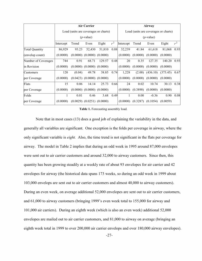
week 8. Table 1 shows the regression results for the five relevant demand attributes.
-27-
Air Carrier Airway
Load (units are coverages or charts) Load (units are coverages or charts)
(p-value) (p-value)
Intercept Trend Even Eight 2r Intercept Trend Even Eight 2r
Total Quantity 86,929 93.23 52,430 51,810 0.88 32,239 41.84 61,618 81,068 0.93
(envelop count) (0.0000) (0.0000) (0.0000) (0.0000) (0.0000) (0.0000) (0.0000) (0.0000)
Number of Coverages 744 0.91 68.71 129.57 0.48 20 0.35 127.35 140.20 0.93
in Revision (0.0000) (0.0000) (0.0000) (0.0000) (0.0000) (0.0000) (0.0000) (0.0000)
Customers 120 (0.04) 49.78 38.85 0.74 1,228 (2.00) (436.10) (373.45) 0.67
per Coverage (0.0000) (0.0423) (0.0000) (0.0000) (0.0000) (0.0000) (0.0000) (0.0000)
Flats 15 0.06 14.14 25.73 0.66 24 0.02 10.74 30.13 0.38
per Coverage (0.0000) (0.0000) (0.0000) (0.0000) (0.0000) (0.3890) (0.0000) (0.0000)
Folds 1 0.01 0.46 3.68 0.49 1 0.00 -0.36 0.90 0.08
per Coverage (0.0000) (0.0029) (0.0251) (0.0000) (0.0000) (0.3287) (0.1054) (0.0059)
Table 1. Forecasting assembly load.
Note that in most cases (13) does a good job of explaining the variability in the data, and
generally all variables are significant. One exception is the folds per coverage in airway, where the
only significant variable is eight. Also, the time trend is not significant in the flats per coverage for
airway. The model in Table 2 implies that during an odd week in 1995 around 87,000 envelopes
were sent out to air carrier customers and around 32,000 to airway customers. Since then, this
quantity has been growing steadily at a weekly rate of about 93 envelopes for air carrier and 42
envelopes for airway (the historical data spans 173 weeks, so during an odd week in 1999 about
103,000 envelops are sent out to air carrier customers and almost 40,000 to airway customers).
During an even week, on average additional 52,000 envelopes are sent out to air carrier customers,
and 61,000 to airway customers (bringing 1999’s even week total to 155,000 for airway and
101,000 air carriers). During an eighth week (which is also an even week) additional 52,000
envelopes are mailed out to air carrier customers, and 81,000 to airway on average (bringing an
eighth week total in 1999 to over 200,000 air carrier envelops and over 180,000 airway envelopes).

-28-
The forecasting model works in a similar way for all five dimensions, so the average number of
subscribers per coverage, for example, decreases from week to week. To generate a demand
scenario for a particular week we use estimates for expected values of the five demand attributes
and their standard errors, and draw a demand scenario from the resulting distribution.
Parameter rw represents the labor cost on resource r, and it is generally well known.
Unfortunately, accurate processing times for the resources t ,p ,ra τ were not as readily available. There
were “standard” processing rates, but they did not represent reality. The problem of determining
accurate processing times is interesting, because the time it takes to assemble a coverage, for
example, depends on several variables: coverage quantity, the number of sections, the number of
folds, and on whether a temporary or a permanent employee performs the work.
Using the manual assembly process as an example, we determined the total processing times
by systematically tracking actual processing and setup times for each coverage over a one week
period. We then fit the following model:
, 1 2 3p assembly p p p p pa folds sections dα β β β ε= + + + + (16)
where αp is the intercept term, foldsp represents the number of folds in coverage p, sectionsp
represents the number of sections in coverage p, dp represents the quantity of coverage p demanded,
and pε is an unobservable random error. Equation (16) gives us an approximation of the total time
in assembly. We fit the model using ordinary least squares. All coefficients were significant, and
the resulting r2 was 78.1%. We determined processing times for other resources using the same
method.
Estimating processing times with the new collator was a more difficult task because we did
not have the opportunity to observe the collator’s performance in the Jeppesen production
-29-
environment. Instead, a team of Jeppesen managers observed the collator’s performance at the
vendor’s site. They collected the production data that we ultimately used to estimate collator
processing times.
For the purpose of the tests, we assume inter-stage independence for the vector of random
parameters t ,τξξξξ . Although demand information at Jeppesen is updated daily, new information
significantly impacts planning only once, on Monday (t = 4) of every week. So a one-week
planning problem is a two stage stochastic model with recourse, where the initial plan is made on
Friday ( 1 1,tτ = = ), production starts and proceeds for three days, demand information is revised on
Monday ( 1 4,tτ = = ), and the plan is adjusted given the new information.
4.2 Comparative Results
To begin our empirical comparison of the three flexibility evaluation approaches, we picked
17 actual consecutive weeks (two complete 8-week cycles, and one additional week following the
second cycle): 21 August 1998 through 11 December 1998. The date 21 August 1998 is the Friday
of week 3, 28 August is the Friday of week 4, 4 September is the Friday of week 5, and so forth.
We had the actual data that went into the revision, and the sequence in which this data was
becoming available to the planning group.
We ran the three models on the 17 weeks of data, which involved solving 17 separate two-
stage stochastic problems. We modeled the current state of the system and the hypothetical system
configuration with the new folder-collator. To determine the benefit of the collator each week, we
take the difference of revision cost with and without the collator. Table 2 compares the SPP
estimates of collator benefit with those of APP and WS. All numbers are presented as percentage
difference with SPP. We estimate ( )SPPV 'R by running 30 replications of Algorithm 1 on a 2-stage
problem.

-30-
Week Percentage Deviation from SPP Date in Cycle WS APP 21-Aug 28-Aug
4-Sep 11-Sep 18-Sep 25-Sep
2-Oct 9-Oct
16-Oct 23-Oct 30-Oct 6-Nov
13-Nov 20-Nov 27-Nov
4-Dec 11-Dec
3 4 5 6 7 8 1 2 3 4 5 6 7 8 1 2 3
0.00 0.09 0.00 0.00 0.00 0.19 0.00
16.67 0.00 0.02 0.00
18.49 25.53 53.27 0.00 4.34 6.09
0.00 60.10 0.00 1.44 0.00
11.23 0.00
22.67 0.00
62.60 1.40
26.85 25.53 76.85 0.00
12.82 21.41
Table 2. Comparative system performance for 17 weeks.
We learn several things from Table 2. First, we see that in every case
( ) ( ) ( )' ' 'APP WS SPPV V V≤ ≤R R R
We also observe that in many of the weeks APP and WS models underestimate the benefit of the
collator relative to SPP. All three models give the same solution in several of the weeks. Those are
all small odd weeks, with low load.
Most of the savings from the collator are due to the two 8th weeks, since the 8th weeks are
the only weeks where internal capacity is insufficient to fulfill demand and an outside vendor is
used for fold assembly. The outside vendor is much more expensive than internal fold assembly,
even if overtime and temporary employees are used. With the new collator, the use of the outside
vendor can be avoided.

-31-
4.3 Estimating the Total Collator Impact
We now compare how the three models estimate the benefit of the new collator over the
three-year planning horizon. The previous section showed that the benefit of this resource increases
with system load.
We estimate the benefit of the collator by simulating the three-year Jeppesen production
environment, based on (15). In other words, we generated 156 weeks of demand consistent with
demand characteristics as presented in Table 1. Each week is a separate two-stage stochastic
model, and the SPP estimates were obtained for each week separately by running 30 replications of
Algorithm 1. Table 3 summarizes average weekly benefit estimates for all three models, along
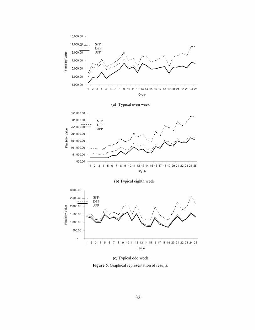
with their standard errors. Figure 6 presents our analysis graphically.
SPP WS APP
Week
Average weekly benefit ($)
(standard error)
Average weekly benefit
(standard error) Deviation from SPP
Average weekly benefit ($)
(standard error) Deviation from SPP
Odd 1,652.71 1,220.67 26.1% 1,164.69 29.5% 393.36 263.29 258.20 Eight 190,086.45 111,280.79 41.5% 88,343.54 53.5% 73,680.73 39,722.19 46,271.29 Even 7,357.41 5,450.43 25.9% 4,735.58 35.6% 1,542.56 884.53 1,344.10
Table 3. Summary of solution results for estimating collator benefit
In the odd week problems, WS and APP results are generally quite close because odd weeks
have low volume, on average, so capacity virtually never becomes an issue. Results look very
different in even and eighth weeks. We clearly see that WS and APP underestimate the benefit of
the collator relative to SPP. In even weeks, APP undervalues the collator by about 36% and WS by
26%. In eighth weeks, APP undervalues the collator by 54% and WS by 41%. In odd weeks, both
APP and WS undervalue the collator by about 26%. All of these differences are highly statistically
significant, using a two sample t-test assuming unequal variances.
-32-
1,000.00
3,000.00
5,000.00
7,000.00
9,000.00
11,000.00
13,000.00
1 2 3 4 5 6 7 8 9 10 11 12 13 14 15 16 17 18 19 20 21 22 23 24 25
Cycle
Flex
ibilit
y Va
lue
(a) Typical even week
1,000.00
51,000.00
101,000.00
151,000.00
201,000.00
251,000.00
301,000.00
351,000.00
1 2 3 4 5 6 7 8 9 10 11 12 13 14 15 16 17 18 19 20 21 22 23 24 25
Cycle
Flex
ibilit
y Va
lue
(b) Typical eighth week
-
500.00
1,000.00
1,500.00
2,000.00
2,500.00
3,000.00
1 2 3 4 5 6 7 8 9 10 11 12 13 14 15 16 17 18 19 20 21 22 23 24 25
Cycle
Flex
ibilit
y Va
lue
(c) Typical odd week
Figure 6. Graphical representation of results.
SPP DPP APP
SPP DPP APP
SPP DPP APP

-33-
Our analysis showed that the annual discounted savings a new collator will generate are
around $1.4 million. Jeppesen accepted our analysis and recommendation, and purchased the
collator in July 1998.
5. Collator Impact
The collator, referred to as “Longford” at Jeppesen, after its manufacturer, was custom-built
and delivered in late December 1998. Figure 7 shows the collator in action at Jeppesen. After an
initial training period, Jeppesen’s assembly area started using the collator on 6 January 1999. We
asked the assembly operations manager to systematically keep track of all work performed on the
collator, which he has accomplished. Table 4 summarizes this data for the period of 8 January 1999
through 21 May 1999, and compares the actual savings with savings forecasted by the three
alternate models.
We determine actual savings each week by considering that week’s entire revision and
determining which coverages should be assembled using the collator. We then compare the actual
cost of assemblying these coverages on the collator, and what it would have cost to manually
assemble them. The difference is in the column labeled “internal” in Table 4. On 8th weeks internal
capacity without the collator is not sufficient to meet the load, so a large number of folds would
have been assembled by an outside vendor. We use the vendor’s actual price schedule to determine
the outsourcing cost that would have been incurred if the collator was not available. This figure is
shown in the column labeled “external” in Table 4.

-34-
Actual Savings Forecasted Savings Week of Cycle Internal External Total APP WS SPP
08-Jan-99 6 477 477 2,657 5,145 5,86515-Jan-99 7 3,322 3,322 1,045 1,085 1,25122-Jan-99 8 2,959 134,728 137,687 28,537 56,365 92,81529-Jan-99 1 22 22 1,478 1,527 1,80105-Feb-99 2 402 402 4,076 6,378 7,17512-Feb-99 3 34 34 1,178 1,261 1,50519-Feb-99 4 661 661 2,572 4,825 5,41126-Feb-99 5 234 234 1,300 1,365 1,65005-Mar-99 6 4,178 4,178 3,537 5,316 6,10112-Mar-99 7 2,583 2,583 1,183 1,200 1,47819-Mar-99 8 7,425 89,679 97,104 28,888 60,521 100,34526-Mar-99 1 0 0 1,465 1,538 1,92802-Apr-99 2 2,021 2,021 4,086 5,559 6,55809-Apr-99 3 0 0 1,550 1,630 2,10416-Apr-99 4 2,647 2,647 4,912 6,334 7,59323-Apr-99 5 529 529 1,040 1,127 1,49530-Apr-99 6 3,854 3,854 6,406 7,314 8,97307-May-99 7 3,625 3,625 1,471 1,531 2,04314-May-99 8 10,317 82,808 93,125 27,737 53,555 93,17221-May-99 1 733 733 933 1,010 1,31628-May-99 2 841 841 4,915 5,640 7,13304-Jun-99 3 19,141 19,141 751 836 1,17311-Jun-99 4 3,130 3,130 5,409 5,815 7,52218-Jun-99 5 7,846 7,846 725 815 1,14225-Jun-99 6 1,582 1,582 4,005 4,541 5,73202-Jul-99 7 7,936 7,936 1,299 1,331 1,94309-Jul-99 8 6,994 68,529 75,523 27,542 51,905 90,72216-Jul-99 1 14,961 14,961 938 986 1,47823-Jul-99 2 6,758 6,758 6,310 6,294 8,19730-Jul-99 3 8,825 8,825 778 809 1,29506-Aug-99 4 0 0 5,901 5,889 7,94613-Aug-99 5 7,600 7,600 718 755 1,15120-Aug-99 6 340 340 4,891 4,843 6,64727-Aug-99 7 1,567 1,567 1,013 1,108 1,63503-Sep-99 8 8,615 72,560 81,175 27,394 69,216 115,58410-Sep-99 1 19,706 19,706 1,381 1,464 2,23917-Sep-99 2 3,909 3,909 4,968 4,937 6,98924-Sep-99 3 18,482 18,482 1,063 1,110 1,74701-Oct-99 4 3,415 3,415 5,317 5,286 7,58408-Oct-99 5 10,481 10,481 1,194 1,230 1,96615-Oct-99 6 4,874 4,874 5,552 5,517 8,16422-Oct-99 7 5,955 5,955 1,579 1,601 2,64029-Oct-99 8 13,510 72,820 86,330 46,190 75,388 120,83405-Nov-99 1 24,136 24,136 1,344 1,365 2,13012-Nov-99 2 24,180 24,180 3,915 3,842 5,60419-Nov-99 3 4,117 4,117 1,160 1,221 1,93926-Nov-99 4 3,223 3,223 5,350 5,321 7,89703-Dec-99 5 2,439 2,439 1,160 1,222 1,96110-Dec-99 6 361 361 5,413 5,372 8,32217-Dec-99 7 8,513 8,513 1,160 1,223 1,98424-Dec-99 8 13,542 78,761 92,303 46,984 84,510 132,95531-Dec-99 1 13,716 13,716 1,160 1,224 2,00607-Jan-00 2 7,623 7,623 5,681 5,667 8,836Total Savings to date: 323,862 599,885 923,748 356,556 587,723 929,812
Table 4. Savings and forecasts over the test period
The internal savings are due to lower cost, in terms of man-hours, for using the collator
instead of the manual assembly method, the increased capacity the collator provides, and increased
decision flexibility the collator offers. The vast majority of the savings, however, are “external,”

-35-
meaning that the collator allowed Jeppesen to bring much of the work in-house that was previously
sub-contracted out to a vendor. These “external” savings illustrate how the collator increased
Jeppesen’s volume flexibility. In an internal memo dated 14 May 1999, Paul Vaughn, the assembly
operations manager wrote: “The bottom line is that the Longford continues to meet expectations
and we are saving dollars!”
Figure 7. Collator in use at Jeppesen
The 53 weeks of data presented in Table 4 demonstrate that our new method for determining
equipment benefit (SPP) is much more accurate in forecasting actual savings than the other two
common methods. SPP estimates are determined by running 30 replications of Algorithm 1 for
each week’s problem, while APP and WS estimates are determined by solving corresponding
deterministic problems. Using a matched pair t-test, we cannot reject with the null hypothesis that

-36-
the SPP forecast and the actual data are the same (p-value = 0.4530). We can reject this null
hypothesis at 1% level for both, APP and WS forecasts (p-value = 0.0006 for APP and 0.0016 for
WS). The mean square error (MES) and bias measures tell the same story. MSE is 613,644,680 for
APP, 250,796,163 for WS and 172,665,224 for SPP. So clearly SPP provides the highest overall
quality forecast. The average bias is -10,661 for APP, -6,252 for WS and 216 for SPP, so both,
APP and WS significantly undervalue the collator, and SPP does not.
The APP model undervalues the Longford, particularly in high-volume 8th weeks in large
part because of aggregation. Since APP does not contain inventory variables to provide links across
periods, it is limited in its ability to properly model systems with limited capacity. But
disaggregating the APP model does not entirely address the problem, because even the
disaggregated model (WS) does not properly model decision flexibility. By increasing volume
flexibility at Jeppesen, the Longford gave management the ability to postpone finalizing production
plan for a few days, until demand becomes known with certainty. The reason our sampling-based
optimization algorithm captures such benefits, and the other two methods do not, is that our method
models how a production system responds to uncertainty.
6. Conclusions
We have demonstrated how some commonly used techniques for evaluating investment
decisions in new production resources can severely under-estimate the benefit of the resources
when the resources provide capacity and decision flexibility. Simple analysis techniques, however,
such as the one developed by Ramasesh and Jayakumar [20] provide a useful benchmark for
analyzing the problem. We see that a simple aggregate method provides a conservative estimate
and can systematically under-estimate the benefit of flexible equipment, sometimes quite
substantially. If a new technology can be justified using a simple conservative method no further

-37-
analysis is required. If, however, a conservative method cannot justify an investment in new
flexible equipment, it may be worthwhile to consider our method to determine the benefit of
flexible equipment more accurately. Naturally, our framework does not guarantee a perfect
estimate for the benefit of flexibility either. No model can systematically account for human error,
for example, so the SPP estimate is likely still a lower bound on the true collator benefit. It is,
however, a more accurate estimate than the two simpler methods, as our results demonstrate.
We applied our method to a real investment problem faced by Jeppesen Sanderson, Inc., the
major aviation information provider in the world. In July 1998, Jeppesen accepted our
recommendation to invest in a new piece of equipment, the Longford folder collator, for its final
assembly department. The Longford was built to Jeppesen specifications, and delivered in
December 1998. Between 6 January 1999 and 7 January 2000, the Longford has been used
consistently, including seven “8th weeks”, generating savings in excess of $900,000. Prior to our
work, the Jeppesen finance department had rejected the Longford proposal, estimating that it would
take six years to pay for itself. As a result of our work they subsequently reversed their decision.
As our model predicted, the Longford has paid for itself in less than six months. The management
was so pleased with this outcome that subsequently, in July 2000 they purchased a second Longford
collator.

-38-
References
[1] Azzone, G. and V. Bertele. 1989. “Measuring the economic effectiveness of flexible automation: a new approach.” International Journal of Production Research, Vol. 27, No. 5, pp. 735-746.
[2] Benjaafar, S., Morin, T. L. and J. Talavage. 1995. “The strategic value of flexibility in sequential decision making.” European Journal of Operational Research, Vol. 82, No. 3, pp. 438-457.
[3] Birge, J. R. and F. Louveaux. 1997. Introduction to Stochastic Programming, Springer Verlag, New York.
[4] Bitran, G. R. and D. Sarkar. 1988. “On upper bounds of sequential stochastic production planning problems.” European Journal of Operational Research, Vol. 34, No. 1, pp. 191-207.
[5] Bitran, G. R. and H. H. Yanasse. 1984. “Deterministic approximations to stochastic production problems.” Operations Research, Vol. 32, No. 2, pp. 999-1018.
[6] Carino, D. R., Kent, T., Myers, D. H., Stacy, C., Sylvanus, M., Turner, A. L., Watanabe, K. and W. T. Ziemba. 1994 “The Russell-Yasuda Kasai model: an asset/ liability model for a Japanese insurance company using multistage stochastic programming.” Interfaces, Vol. 24, No. 1, pp. 29-49.
[7] Das, S. and P. Nagendra. 1993. “Investigations into the impact of flexibility on manufacturing performance.” International Journal of Production Research, Vol. 31, No. 11, pp. 2337-2354.
[8] de Groote, X. 1994. “The Flexibility of Production Processes: A General Framework,” Management Science, Vol. 40, No. 7, pp. 933-945.
[9] Eppen, G. D., Martin, R. K and L. Schrage. 1989. “A scenario approach to capacity planning.” Operations Research, Vol. 37, No. 4, pp. 517-527.
[10] Fine, C. and R. Freund. 1990. “Optimal investment in product-flexible manufacturing capacity.” Management Science, Vol. 36, No. 4, pp. 449-466.
[11] Gerwin, D. 1993. “Manufacturing flexibility: a strategic perspective." Management Science, Vol. 39, No. 4, pp. 395-410.
[12] Goldratt, E. M. and J. Cox. 1992. The Goal. North River Press, Inc., Great Barrington.
[13] Gupta, D., Gerchak Y. and J. Buzacott. 1992. “The optimal mix of flexible and dedicated manufacturing capacities: Hedging against demand uncertainty.” International Journal of Production Economics, Vol. 28, No. 3, pp. 309-319.
[14] Gupta, Y. P. and S. Goyal. 1989. “Flexibility of manufacturing systems: concepts and measurements,” European Journal of Operational Research, Vol. 43, pp. 119-135.
[15] Infanger, G. 1993. Planning Under Uncertainty: Solving Large-Scale Stochastic Linear Programs. The Scientific Press.
[16] Jordan, W.C. and S. C. Graves. 1995. “Principles on the benefits of manufacturing process flexibility.” Management Science, Vol. 41, No. 4. pp. 577-594.

-39-
[17] Katok, E. 1996. “Planning manufacturing flexibility in an uncertain production environment: general framework and implementation.” Unpublished Ph.D. Dissertation, The Pennsylvania State University.
[18] Katok, E., Tarantino, W. and R. Tiedeman. 2001 “Flexibility Planning and Technology Management at Jeppesen Sanderson, Inc.” Interfaces, Vol. 31, No. 1, pp. 7-29.
[19] Mulvey, J.M., Gould, G. and C. Morgan. 2000. “An asset and liability management system for Towers Perrin-Tillinghast.” Interfaces, Vol. 30, No. 1, pp. 96-114.
[20] Ramasesh, R.V. and M. D. Jayakumar. 1997. “Inclusion of flexibility benefits in discounted cash flow analyses for investment evaluation: A simulation/optimization model.” European Journal of Operational Research, Vol. 102, pp. 124-141.
[21] Sethi, K.S. and S.P. Sethi. 1990. “Flexibility in manufacturing: a survey.” The International Journal of Flexible Manufacturing Systems, Vol. 2, pp. 289-328.
[22] Sinha, D. and J. Wei. 1992. “Stochastic analysis of flexible process choices.” European Journal of Operational Research, Vol. 60, No. 2, pp. 183-199.
[23] Smith, J.E. and K. F. McCardle. 1998. “Valuing oil properties: integrating options pricing and decision analysis approaches.” Operations Research, Vol. 46, No. 2, pp. 198-217.
[24] Smith, J.E. and R. F. Nau. 1995. “Valuing risky projects: option pricing theory and decision analysis.” Management Science, Vol. 41, No. 5, pp. 795-816.
[25] Suarez, F.F., Cusumano, M.A. and C. H. Fine. 1996. “An empirical study of manufacturing flexibility in printed circuit board assembly.” Operations Research, Vol. 44, No. 1, pp. 223-240.
[26] Suresh, N.C. 1990. “Towards an integrated evaluation of flexible automation investments.” International Journal of Production Research, Vol. 28, No. 9, pp. 309-319.
[27] Upton, D.M., 1994. “The management of manufacturing flexibility," California Management Review, Winter, pp. 72-89.
[28] van Mieghem, J.A. 1998. “Investment strategies for flexible resources.” Management Science, Vol. 44, No. 8, pp. 1071-1078.