1

Hochschule Neubrandenburg

Fachbereich Landschaftswissenschaften und Geomatik

Studiengang Geodäsie und Geoinformatik

Investigations to digitizing of the gyro oscillation

swing by a line camera

Master’s thesis

presented by: Yaroslav Lopatin

for obtaining the academic degree

"Master of Engineering" (M.Eng.)

Examiner: Prof. Dr.-Ing. Wilhelm Heger

Second Examiner: Prof. Dr. Tech. Sc Anatoliy Tserklevych

Submitted on: 02.07.2018

URN: nbn: de: gbv: 519-thesis 2018 - 0043 - 2

2

Declaration for the Master’s Thesis I confirm that this Master's thesis is my own work and I have documented all sources and material

used. This thesis was not previously presented to another examination board and has not been

published.

____________________________

____________________________

Place and date Signature

3

ANNOTATION

Yaroslav Lopatin

Investigations to digitizing of the gyro oscillation swing by a line camera

Studiengang Geodäsie und Geoinformatik

Hochschule Neubrandenburg

Neubrandenburg 2018

This Master thesis considers development of a software program for automation of a gyro

measurement process.

The master thesis includes the following sections:

1.Introduction

2. Methodology

3. Implementation

4. Conclusions

The result of this work is a programming software that allows to control the line camera and

calculate the necessary values for getting the azimuth value that can be used for automation of the

gyro measurement procedure.

This Master thesis contains 6 tables, 26 figures, 11 formulas, 3 appendixes.

Keywords: gyro, line camera, software, automation.

4

Table of content ABSTRACT............................................................................................................... 5

1. Introduction ............................................................................................................ 6

1.1 History.........................................................................................................................................6

1.2. Gyro measurement principles ..................................................................................................16

1.3 Existing gyros ...........................................................................................................................21

1.4 Reasons for new development ..................................................................................................30

2. Methodology .........................................................................................................31

2.1 Observation methods ................................................................................................................31

2.2 Objectives .................................................................................................................................35

2.3 Line camera...............................................................................................................................35

2.4 Control computer ......................................................................................................................40

2.5 Programming language .............................................................................................................42

3. Implementation ......................................................................................................44

3.1 Workflow ..................................................................................................................................44

3.2 Testing the program ..................................................................................................................53

Conclusions ...............................................................................................................54

References.................................................................................................................56

5

ABSTRACT

A method for digitizing of the gyro oscillations for automation of the gyro measurements

using a camera with a linear sensor camera and programming code is proposed in this work. Also it

analyzes the history of gyro designing from the invention to the modern automated devices.

The main goal of this work is to develop a technology for automatically determining the

position of a light source and further computation of the necessary data with the possibility of

application in a gyroscope. The accuracy of determining of principal values should be higher than

by manual procedure.

The working possibility of the line camera from Coptonix company was investigated, as

well as the possibility of its connection to a single board computer Raspberry Pi 3B for data

transmission and processing. The possibility of using the Python programming language for higher

tasks was tested.

The result of this work is the creation of software using the programming language Python,

which connects the user to the linear camera, records the necessary data, transfers them to the

client-computer and calculates the necessary values. For the convenience of using the program by

other users, the program is provided with GUI. The result of the program is a file with the extension

.xml, which contains data about measurements.

This technology was tested using a special facility that simulates the oscillation of the light

bar in the gyroscope. In the future, this technology can be implemented with a gyro model Gyromax

AK-2M, which will make it possible to automate this device, greatly simplifying the measurement

procedure and also increasing the accuracy of measurements due to the high accuracy of the linear

camera and eliminating the observer error.

6

1. Introduction

1.1 History

The word "gyroscope" can be translated as a "rotation observer". A gyroscope is a device

capable of responding to a change in the angles of the orientation of the body on which it is

mounted relative to the inertial reference frame. A term was first introduced by J. Foucault in his

report in 1852 in the French Academy of Sciences [1]. The report was dedicated to the methods of

experimental detection of the Earth’s rotation in the inertial space. This is the reason for the name

“gyroscope”.

Before the invention of the gyroscope, mankind used various methods of determining the

direction in space. For a long time, people orientate visually by remote objects, in particular, by the

Sun. Already in ancient times appeared the first instruments based on gravity: the plumb line and

the level. In the Middle Ages, a compass was invented in China, using the Earth’s magnetism. In

ancient Greece, astrolabes and other instruments based on the position of stars were created.

The gyroscope was invented by Johannes Bohnenberger and published the invention in 1817

[7]. The main part of the Bohnenberger gyro was a rotating massive ball in the cardan suspension.

In 1852 the French scientist Foucault improved the gyroscope and first used it as an instrument

showing a change in direction (in this case – the Earth). The advantage of the gyroscope over older

instruments was that it operated correctly in difficult conditions (poor visibility, jolting,

electromagnetic interference). However, the rotation of the gyroscope down due to the friction. In

the second half of the XIX century it was proposed to use an electric engine to accelerate and keep

the rotation of the gyroscope.

The development of gyroscopic technology has led to the fact that a very wide class of

instruments has been called that way, and now the term "gyroscope" is used to refer to devices

containing a material object that performs rapid periodic rotations.

In our time, not a single geodetic-mining work, no moving object, either a fishing boat or a

complex spacecraft, does not functioning without gyroscopic instruments. They are widely used in

navigation is seafaring, aircraft and astronautics. Most of the offshore sea vessels have a gyro

compass for driving control of the ship, some of them have gyrostabilizers. Gyroscope is necessary

for good automated controlling of missiles. All aircrafts are supplied with gyro devices, with the

help of which they receive reliable information for stabilization and navigation systems. For

example, an air horizon, a gyrovertical, a gyroscopic index of roll, pitch and yaw. Gyroscopes can

be either pointing instruments or autopilot sensors.

7

In addition to air and naval forces, gyroscopes are used in artillery and missile forces in the

army. Also gyroscopes serve to determine the azimuth of the orientated direction and are widely

used in surveying, geodesy, topography, mining, for orienting tunnels and mines. The main type of

gyroscope in this area is the gyrotheodolite, which uses the Foucault compass principle.

Gyrotheodolites have a high accuracy in measurements ranging from units of angular

minutes to several units of angular seconds. Even nowadays, when GPS equipment supersedes

optical geodetic devices, it is impossible to do without gyrotheodolites in some areas.

The history of the gyroscopic orientation method, which is very young compared to others,

dates back to the nineteenth century, when seafarers more often needed a more precise orientation

during the journey.

Before the invention of the gyroscope, mankind used various methods for determining the

direction in space. For a long time, people have been oriented towards in the distant objects, along

the Sun, the stars. In the Middle Ages, a compass was invented in China, using the Earth's magnetic

field. In Europe, there were created astrolabes and other instruments based on orientation relative to

the stars. In 1852 Foucault described a new device and called it a gyroscope. This device made it

possible to reproduce the inertial coordinate system and determine the direction of the Earth's

rotation axis. Seafarers did not always fully trust shipborne compasses. For example, cases were

known, when lightning struck the ship and both compasses on the ship turned out to be

"remagnetized". Compass readings were affected by magnetic anomalies and simply by ordinary

metal objects that happened to be near him. Unexpected decision was proposed by Foucault

himself. He proved: if the three-degree gyroscope is deprived of one degree of freedom, and the

remaining free axis of the cardan ring is installed vertically, then the axis of rotation of the flywheel

itself will come to the plane of the meridian. This will happen because it is in the plane of the

meridian, that the horizontal component of the Earth's rotation speed lies.

So, if a magnetic compass uses the earth's magnetic field for its work, then the gyroscopic

compass uses the effect of the Earth's rotation. But when the device was installed on the deck of the

ship, a strange phenomenon was discovered: the axis ceased to come to a stable position, it made

continuous chaotic oscillations in the horizontal plane. This was due to the pitching of the ship. The

gyroscope with three degrees of freedom carried relatively smoothly the rolling, keeping the

direction of the axis of rotation of the flywheel in the absolute space - this was known to many

scientists and engineers. But how to "tie" the axis of rotation of the flywheel to the plane of the

earth's meridian was unclear.

The good idea is to specifically cause the precession of the rotation axis of the flywheel,

forcing it to come into the plane of the meridian, and then, remaining in this plane, spinning along

8

with it in absolute space - first came to the head of the Dutch priest Maxim Gerrard Van den Bos. In

1886, he received a patent for an application entitled "New Ship Compass". The proposal of Van

den Bos was very simple. In the three-degree Foucault gyroscope, the center of mass coincided with

the point of intersection of the axes of the cardan suspension and the axis of the flywheel's own

rotation. Van den Bos suggested that the center of mass of the gyroscope be lowered somewhat

below the axis of the inner ring of the cardan suspension. This was the solution to the problem [8].

Little by little, through the efforts of many scientists, engineers and technologists,

gyroscopic instruments have been significantly improved. In the second half of the XIX century, it

was suggested to use an electric motor to accelerate and maintain the gyro's motion.

For the first time in practice, gyroscope was used in the 1880s by the Aubrey engineer to

stabilize the torpedo course. In the twentieth century, gyroscopes began to be used in airplanes,

rockets and submarines instead of the compass or with it [3].

To create gyroscopes of a modern type, it took more than a decade. In the twentieth century,

the accuracy in precise measurements has increased more and more. Not only the army and the

navy developed, but also coal mining, mining in general, transport, tunnels. Attempts were made to

develop a gyroscopic compass that could satisfy the needs of mine surveying to ensure the accuracy

of underground cross-cuts.

As in any industry, the inventors suffered many setbacks before creating a reliable and

convenient device. Immediately to design the ideal gyroscope was not possible. In addition, the

problem of the historical development of gyroscopic equipment is that initially when creating

gyroscopes other purposes were pursued. These were instruments primarily for the fleet and for the

army (mainly artillery). But thanks to the sailors, the surveyors got a gyrocompass and gyro-sextant,

and thanks to the artillerymen - a gyro-boussole. Elmer Sperry from US visited Europe many times

in the early 1900´s. He was taking ideas from German and other European companies, especially

from Anschütz for his own gyroscope inventions. His company was founded in 1910 and today still

on the market. In 1914 he won a price in Paris for a stabilized airplane flight. The WW I made him

a lot of contracts for torpedo, ship and airplane navigation/steering [9].

At the same time, in the USSR in the 1930s were also held researches on the creation of

gyrocompasses, and in 1936, the Leningrad Institute of Fine Mechanics (LITMO) in the Faculty of

Fine Mechanics and Optics has opened two new branches: navigation instruments and calculating

devices. There were developed prototypes of gyrocompass and gyro-boussole, but they proved to be

completely inapplicable in geodesy and mine surveying [10]. And only after the Second World

War, both countries - the USSR and Germany - returned to the idea of creating a "ground" gyro. In

the USSR, all the works were concentrated in the All-Union Scientific Research Mine Survey

9

Institute (VNIMI) under the direction of P.L. Ilyin [10], and in FRG similar work was carried out at

the Clausthal Mining Academy under the direction of Professor O. Rellensman [11].

Finally, in 1950, the Soviet mine surveyor gyrocompass M-1 was released. Approximately

at the same time in FRG independently constructed a similar device - the indicator of meridian

MW1 (Meridian Weiser). The creation of the first surveying gyroscopes marked the beginning of

the practical use of the method of gyroscopic orientation in geodesy and in mine surveying. This

was a big breakthrough not only in theory, but also in practice. After all, with the help of M-1, more

than fifty mines have been produced in the Donbas, Kryvyi Rih and Kuzbas. Scientists and

engineers began to work with renewed enthusiasm and for several years the engineers of both

countries developed and improved several models (M-3 and MUG-2, B2B), which were

subsequently used in practice. With their help, they found deviations in the orientation of some

mines. This concludes the first stage of the creation of gyroscopic instruments. And although they

had a number of drawbacks - cumbersomeness, a huge mass (about 500-600 kg), large energy costs,

but finally approved the belief in the gyroscopic method as a reliable method of geodetic and mine

surveying. The measurement time of M-3 model was approximately 30 minutes with accuracy of

1’15’’. MUG-2 model had measurement time of 29 minutes and accuracy of 1’30’’ [10].

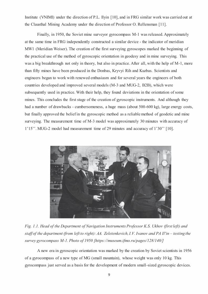
Fig. 1.1. Head of the Department of Navigation Instruments Professor K.S. Ukhov (first left) and

staff of the department (from left to right): AA. Zeletenkevich, I.V. Ivanov and PA Il'in – testing the

survey gyrocompass M-1. Photo of 1950 [https://museum.ifmo.ru/pages/128/140/]

A new era in gyroscopic orientation was marked by the creation by Soviet scientists in 1956

of a gyrocompass of a new type of MG (small mountain), whose weight was only 10 kg. This

gyrocompass just served as a basis for the development of modern small-sized gyroscopic devices.

10

The intermediate goal – to develop a portable and transportable device – was achieved. Such

a "light" gyrocompass made it possible to carry out measurements in inaccessible conditions. In

1957, was completed the work on the design of the first model of the device in explosion-proof

design - the mine surveyor gyrocompass MV1 (later - MV2). In a similar scheme, a portable

surveying gyrocompass in explosion-proof design MV2M with a semiconductor converter was

created. In Germany, in contrast to the USSR, during this period a gyrocompass with a torsion

suspension was developed. This design was very successful, as it ensured high accuracy and

productivity of gyroscopic azimuth measurement with low weight, dimensions and energy costs.

In 1957, the development of a model of a surveying gyro compass with torsion suspension

TV4 was completed. In 1958 the firm Fennel released torsion gyrotheodolite KT-1

(Kreiseltheodolit), and further - the advanced models of KT-2, MW10, MW7, MW50, MW77 and

gyro add-on TK-4, TK-5 [12]. Since the early 60's. in the USSR, began to design the torsion

gyrocompass too, which was released in 1963 under the brand MT1. In 1967, was completed the

work on a small-sized compass MW2, which is the first sample of an explosion-proof surveying

gyro compass with a torsion suspension of a sensitive element. Both models contributed to

achieving higher accuracy of gyroazimuth measurement, and MWT2 became the most widespread

surveying gyrocompass on for more than twenty years. MW2 was a device with an automatic

tracking system for the position of diversion points intended for autonomous determination of the

azimuth of the direction with an error of 30". At the same time, the time required for a single

definition of azimuth at four points of reversion was 20-30 minutes.

In the future, the designers worked on the improvement of portable gyrocompasses with a

torsion suspension: in 1970 a gyrocompass MTV4 was created, and in 1975 - the gyro-boussole, in

which all the components necessary for the work (the gyroblock, the measuring unit and the power

unit) were combined into one unit.

11

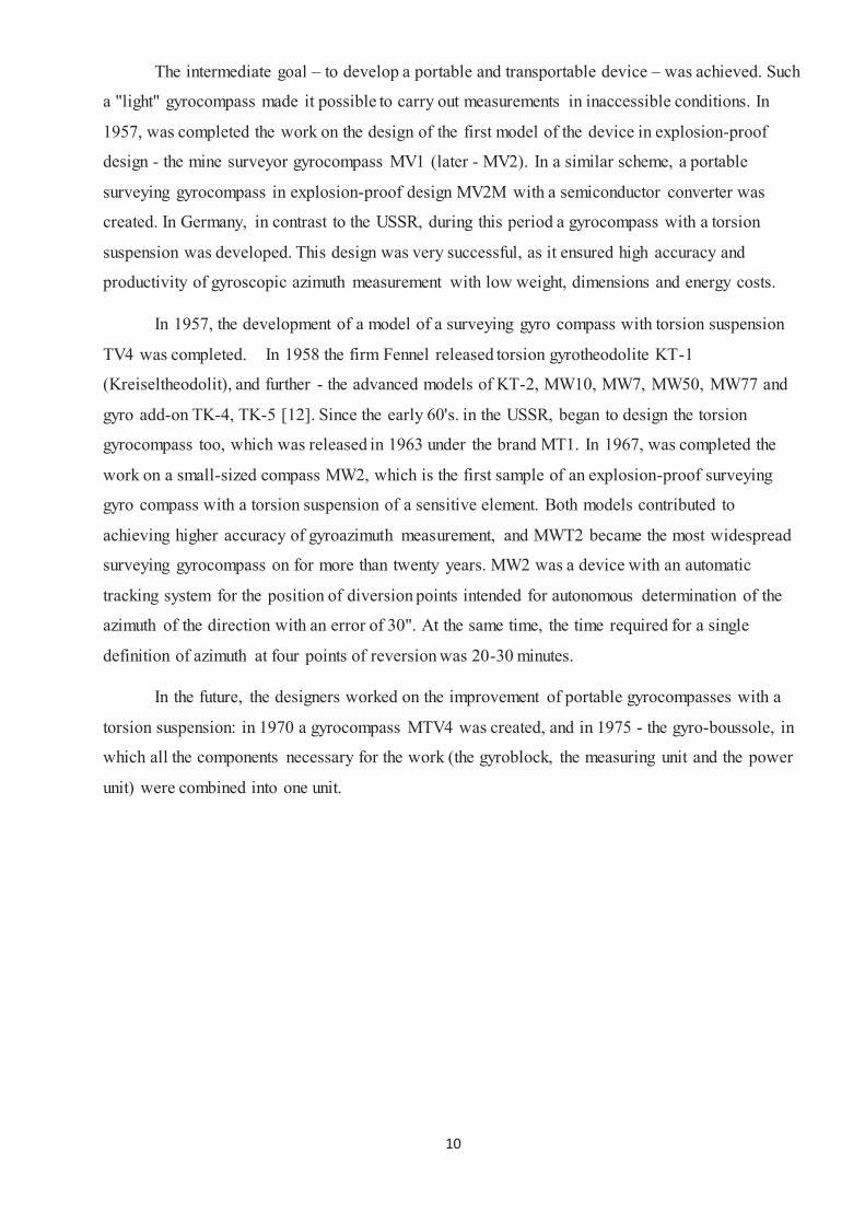
Fig. 1.2. Mine surveying gyrocompass MWT-2: 1 - measuring block; 2 - the gyroblock; 3 - a tripod;

4 - case; 5 - power supply unit (semiconductor converter and battery)

[http://biblioclub.ru/index.php?page=book&id=65325]

In the Soviet Union and the CMEA countries, the need for gyroscopic equipment increased:

new mines, metro stations were built in Moscow, Leningrad, Kiev, Minsk, railway tunnels, and

large hydro units. Missile troops and artillery also needed these devices. The world market for

geodetic and surveying equipment has also expanded rapidly. In 1959, the first model of the

operating ground artillery gyrocompass (under the cipher AG) and the first model of the geodesic

gyrocompass (gyrotheodolite GT-1, later GT-2) were created in the USSR on the basis of the mine

gyro compass MG. Soon specialists from Hungary started to develop gyrotheodolites, who in the

60's created the Gi-B1 gyrotheodolite, Gi-C1, Gi-C2 gyro and Gi-B2 gyrocompass. On the basis of

the latter, Hungarian engineers constructed the Gi-B21 gyrotheodolite, which has an automatic

fixation and the results of measurements on the light panel, and in 1978 - the gyrotheodolite Gi-

B2M, then Gi-B3. The Hungarian Optical and Mechanical Combine (MOM) was engaged in the

manufacture of devices. The Gi-B2M device consisted of three main units: the goniometer part, the

gyroscope and the power supply unit. The goniometric part - the modernized Te-B1 theodolite with

built-in autocollimation system - was designed to measure the angles and observe the points of

variation of the harmonic vibrations of the sensitive element. The sensor of the direction of the

meridian was a pendulum gyroscope with a torsion suspension of the sensitive element [10].

12

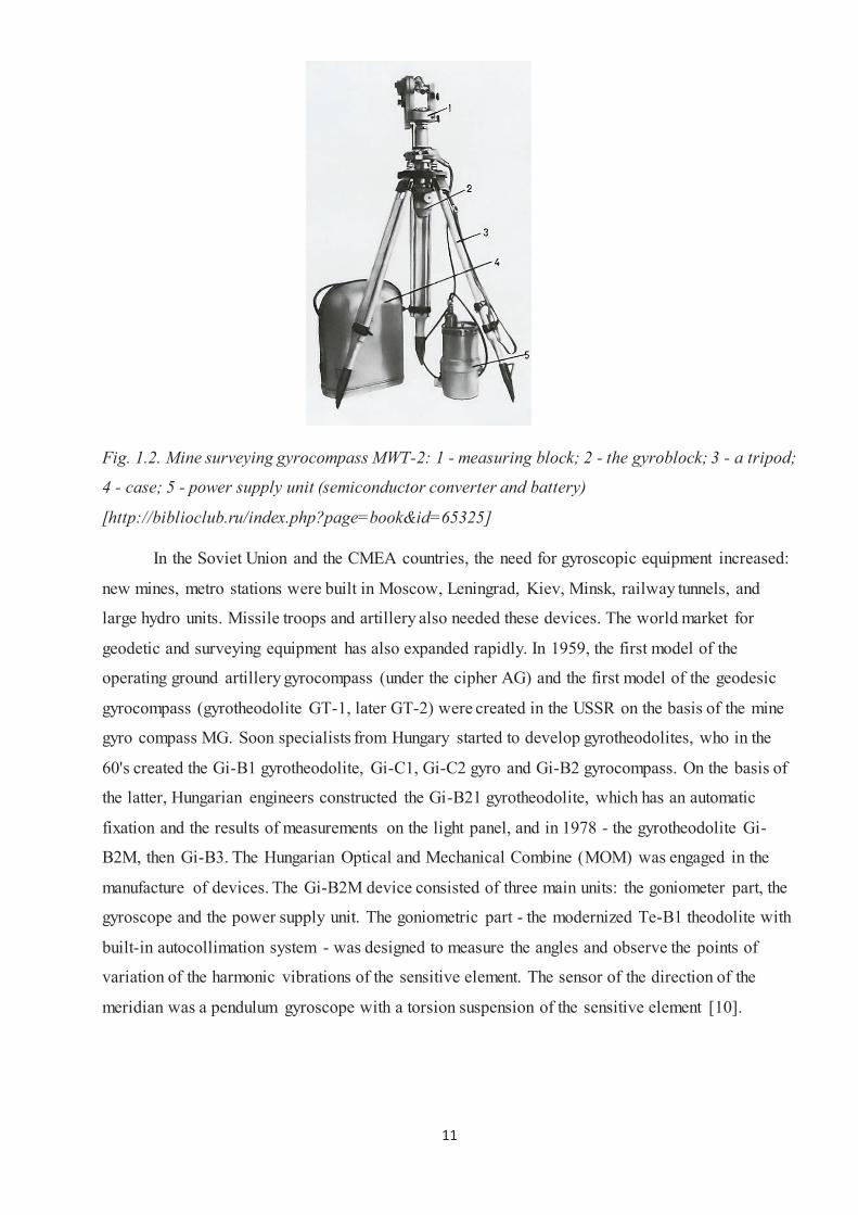
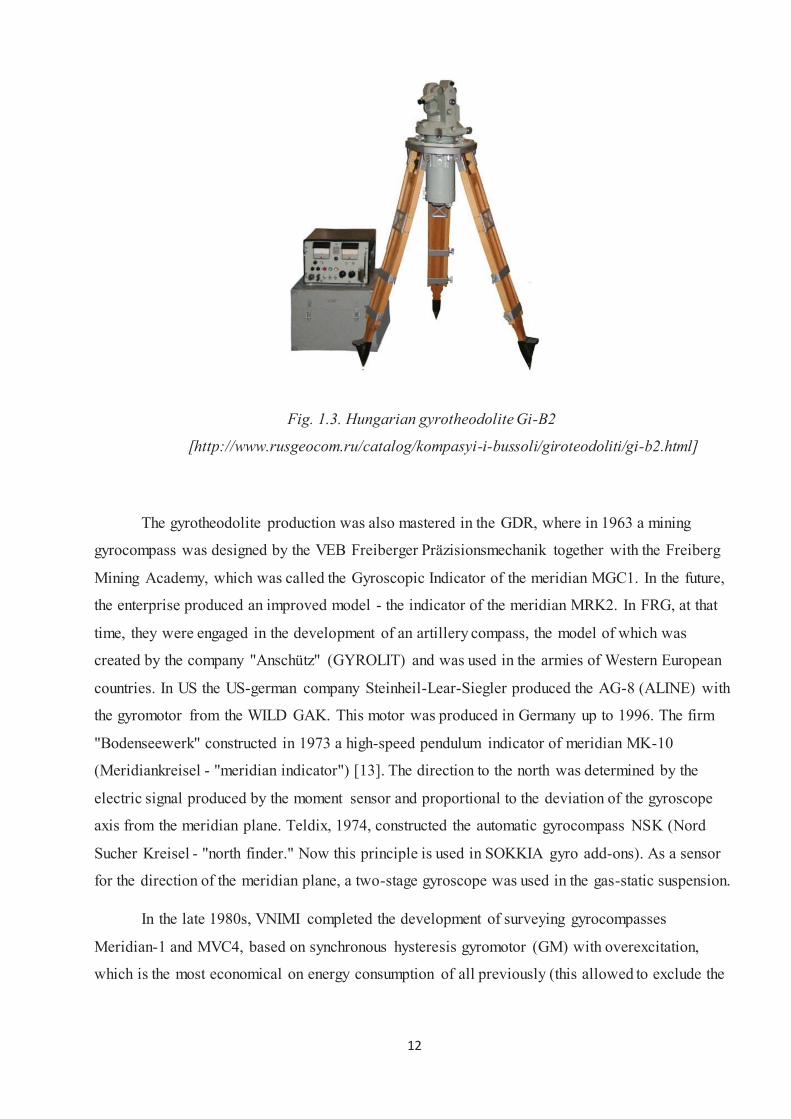
Fig. 1.3. Hungarian gyrotheodolite Gi-B2

[http://www.rusgeocom.ru/catalog/kompasyi-i-bussoli/giroteodoliti/gi-b2.html]

The gyrotheodolite production was also mastered in the GDR, where in 1963 a mining

gyrocompass was designed by the VEB Freiberger Präzisionsmechanik together with the Freiberg

Mining Academy, which was called the Gyroscopic Indicator of the meridian MGC1. In the future,

the enterprise produced an improved model - the indicator of the meridian MRK2. In FRG, at that

time, they were engaged in the development of an artillery compass, the model of which was

created by the company "Anschütz" (GYROLIT) and was used in the armies of Western European

countries. In US the US-german company Steinheil-Lear-Siegler produced the AG-8 (ALINE) with

the gyromotor from the WILD GAK. This motor was produced in Germany up to 1996. The firm

"Bodenseewerk" constructed in 1973 a high-speed pendulum indicator of meridian MK-10

(Meridiankreisel - "meridian indicator") [13]. The direction to the north was determined by the

electric signal produced by the moment sensor and proportional to the deviation of the gyroscope

axis from the meridian plane. Teldix, 1974, constructed the automatic gyrocompass NSK (Nord

Sucher Kreisel - "north finder." Now this principle is used in SOKKIA gyro add-ons). As a sensor

for the direction of the meridian plane, a two-stage gyroscope was used in the gas-static suspension.

In the late 1980s, VNIMI completed the development of surveying gyrocompasses

Meridian-1 and MVC4, based on synchronous hysteresis gyromotor (GM) with overexcitation,

which is the most economical on energy consumption of all previously (this allowed to exclude the

13

instrument correction of the gyrocompass and significantly increased the productivity of work on

gyroscopic orientation).

The first domestic explosion-proof gyrocompass, in which the process of determining the

gyroscopic azimuth of the oriented side was automated, was the surveying gyrocompass MVC4.

The gyroscopic azimuth in the device was calculated automatically by signals from the digital angle

sensor during one precessional oscillation period, and the result was displayed on a digital display.

But gyrocompasses MVTS4 and Meridian-1 were not produced serially.

It is also necessary to note the developments of Ukrainian scientists of the Kiev plant

"Arsenal" - automated high-precision gyro-theodolites of the GT and UGT series, which were used

to determine astronomical azimuths of reference directions in geodesy, construction, and in the

armed forces [2].

In the future, there was a need to improve and develop high-precision digital

gyrocompasses, which do not require a regular determination of the instrument offset on the one

hand, and the development of gyroscopes of technical accuracy, small size, that differ in the

simplicity of manufacture and operation, on the other. From this moment, the use of a modern

element base begins: a synchronous hysteresis gyro-motor with an end mirror surface, a

microprocessor for the processing of measurement information, a digital goniometer, etc. New

requirements are also imposed on the new instruments: high accuracy, minimum time spent on

measurements, simplicity and ease of maintenance. However, with the application of the satellite

system for determining the coordinates on the earth's surface (GPS) into all fields of activity, the

military immediately declined from gyroscopic developments, assessing the simplicity of GPS. This

led to a halt in developments in the civil sphere. The popularity of gyroorientation has dropped

significantly, gyro appliances have ceased to be used for ground operations, and accordingly - and

to release.

But for mine surveying work, the gyroscopic orientation method has remained the main and

reliable method, providing accuracy in underground conditions. Therefore, in our time, the

development of gyroscopic devices takes into account, first of all, the requirements of surveying

services. Gyro-instruments of technical accuracy with medium standard deviation of the azimuth

determination of the side 2-3' is applied in complex mining and geological conditions, including in

the orientation of mine excavations. With the help of gyrotheodolites with the standard deviation of

the determination of azimuth 3-10 " was done a cross-cut of a 50-kilometer tunnel under the English

Channel linking England with France [2].

The history of the development of the gyro equipment gradually evolved to its main goal -

the creation of such gyroscopic instruments that would provide reliability and accuracy in complex

14

underground conditions during mine surveying. Today, the main manufacturers of gyroscopic

instruments are Germany and Japan. In Japan, SOKKIYA produces gyro add-ons GP1, the

operating principle of which is based on the property of a suspended gyro pendulum to oscillate

with respect to the earth's meridian ("true northward"), which are caused by the rotation of the

Earth. This principle is called the North Seeking Gyroscope. The determination of the direction to

the north is made with the standard deviation = ± 20 "at latitudes up to 75 °. The weight of the set-

top box, which is mounted on top of the electronic theodolite or total station, is only 3.8 kg [14].

German company DMT, engaged in the production of gyro appliances, is known for the

creation of GYROMAT-2000 (and its advanced version GYROMAT-3000&5000) the "gold

standard" for geodetic-mining measurements during tunnel cross-cuts. Since entering the market to

this day, engineers around the world have called GYROMAT the best gyro, fully automated and

possessing excellent characteristics. None of the existing gyros created before did not provide such

accuracy and rapidity of measurements. The only disadvantage of this system is its price. From

1989 DMT produced a Gyrotheodolite (GYRO-STATION) for SOKKIA/Japan with an optical

adaptation between total station and gyroscope (all DMT gyros invented by Reinhard Schäfler) .

German company GMT (GeoMessTechnik) has created the technology GYROMAX.

GYROMAX AK-2M - gyroscopic add-on that works on the basis of electronic total stations of the

world's leading manufacturers of geodetic equipment - Leica, Topcon, Trimble, Zeiss and others.

Base of the system is the WILD-GAK motor and the GAK functional principle that was used also in

other German products.

The goal of this product is the replacement for the worldwide used GAK gyroscope with a mid-

accuracy (SAZI<20”) and low price.

Summarizing the above, it should be noted that modern gyroscopic equipment is

distinguished by high accuracy of measurements and convenience in use, modern instruments have

become many times smaller and lighter. At the moment, several dozens of devices have been

developed, with the help of which the gyroscopic orientation can be done in the most difficult

conditions. And while satellite technology is being used for surveying and navigation on the

surface, in mine surveying - in the construction of tunnels, mines, collectors and other underground

objects - without gyroscopes it’s impossible to do. After all, GPS just does not work underground.

In addition, some military are inclined to believe that GPS can refuse to work in case of military

action. Or the US as a global navigation system operator can significantly limit the use of signals

during the period of hostilities. And only with the help of gyroscopic devices, engineers will be able

to make tunneling, and the military will correctly calculate the direction [2].

15

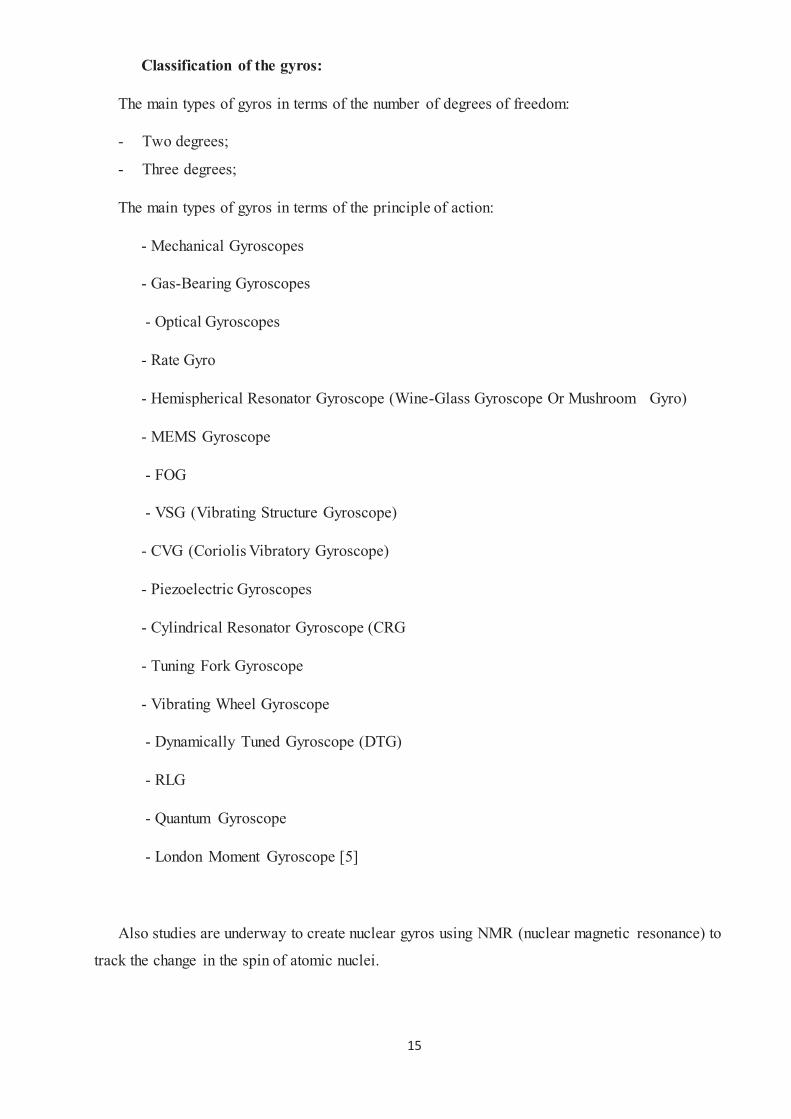
Classification of the gyros:

The main types of gyros in terms of the number of degrees of freedom:

- Two degrees;

- Three degrees;

The main types of gyros in terms of the principle of action:

- Mechanical Gyroscopes

- Gas-Bearing Gyroscopes

- Optical Gyroscopes

- Rate Gyro

- Hemispherical Resonator Gyroscope (Wine-Glass Gyroscope Or Mushroom Gyro)

- MEMS Gyroscope

- FOG

- VSG (Vibrating Structure Gyroscope)

- CVG (Coriolis Vibratory Gyroscope)

- Piezoelectric Gyroscopes

- Cylindrical Resonator Gyroscope (CRG

- Tuning Fork Gyroscope

- Vibrating Wheel Gyroscope

- Dynamically Tuned Gyroscope (DTG)

- RLG

- Quantum Gyroscope

- London Moment Gyroscope [5]

Also studies are underway to create nuclear gyros using NMR (nuclear magnetic resonance) to

track the change in the spin of atomic nuclei.

16

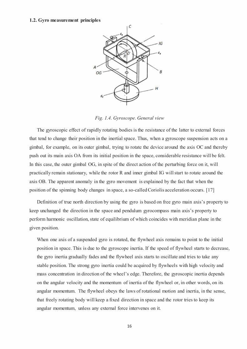
1.2. Gyro measurement principles

Fig. 1.4. Gyroscope. General view

The gyroscopic effect of rapidly rotating bodies is the resistance of the latter to external forces

that tend to change their position in the inertial space. Thus, when a gyroscope suspension acts on a

gimbal, for example, on its outer gimbal, trying to rotate the device around the axis OC and thereby

push out its main axis OA from its initial position in the space, considerable resistance will be felt.

In this case, the outer gimbal OG, in spite of the direct action of the perturbing force on it, will

practically remain stationary, while the rotor R and inner gimbal IG will start to rotate around the

axis OB. The apparent anomaly in the gyro movement is explained by the fact that when the

position of the spinning body changes in space, a so-called Coriolis acceleration occurs. [17]

Definition of true north direction by using the gyro is based on free gyro main axis’s property to

keep unchanged the direction in the space and pendulum gyrocompass main axis’s property to

perform harmonic oscillation, state of equilibrium of which coincides with meridian plane in the

given position.

When one axis of a suspended gyro is rotated, the flywheel axis remains to point to the initial

position in space. This is due to the gyroscope inertia. If the speed of flywheel starts to decrease,

the gyro inertia gradually fades and the flywheel axis starts to oscillate and tries to take any

stable position. The strong gyro inertia could be acquired by flywheels with high velocity and

mass concentration in direction of the wheel’s edge. Therefore, the gyroscopic inertia depends

on the angular velocity and the momentum of inertia of the flywheel or, in other words, on its

angular momentum. The flywheel obeys the laws of rotational motion and inertia, in the sense,

that freely rotating body will keep a fixed direction in space and the rotor tries to keep its

angular momentum, unless any external force intervenes on it.

17

But there is one exception: when the spin axis is oriented to the polar star, it doesn’t move

relative to the observer, because of the fact, that the axis is parallel to the Earth’s spin axis and

oriented to the Celestial poles.

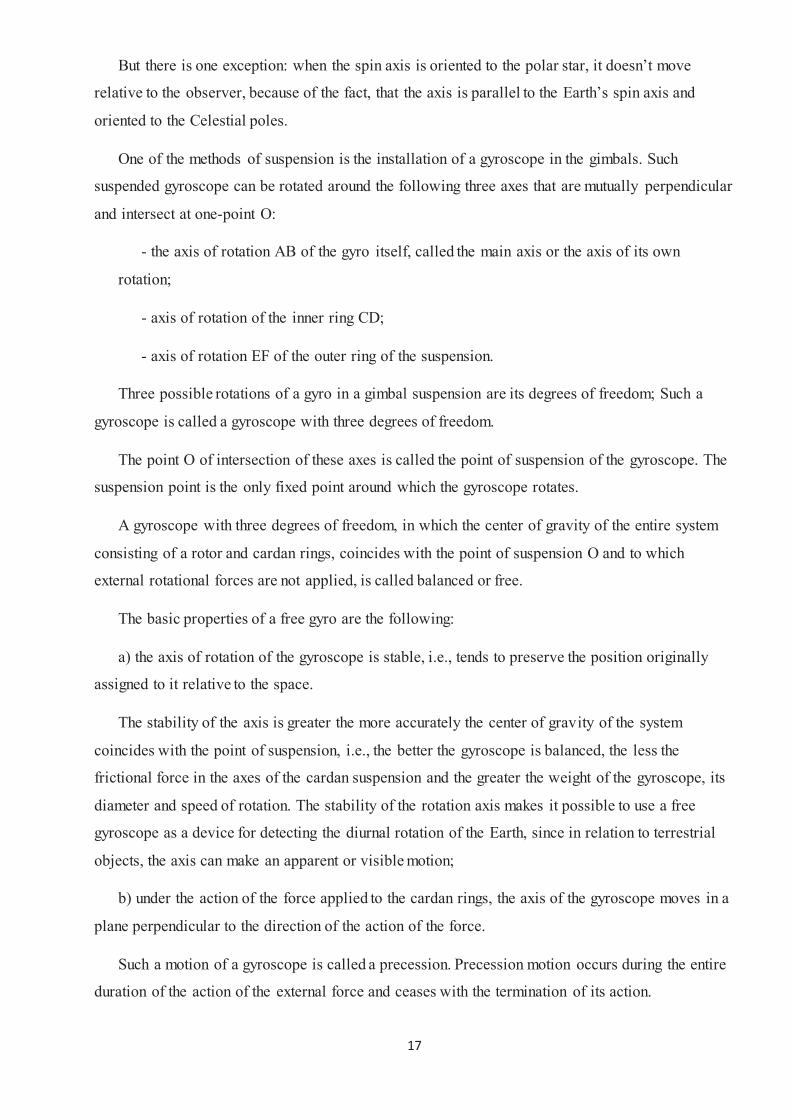
One of the methods of suspension is the installation of a gyroscope in the gimbals. Such

suspended gyroscope can be rotated around the following three axes that are mutually perpendicular

and intersect at one-point O:

- the axis of rotation AB of the gyro itself, called the main axis or the axis of its own

rotation;

- axis of rotation of the inner ring CD;

- axis of rotation EF of the outer ring of the suspension.

Three possible rotations of a gyro in a gimbal suspension are its degrees of freedom; Such a

gyroscope is called a gyroscope with three degrees of freedom.

The point O of intersection of these axes is called the point of suspension of the gyroscope. The

suspension point is the only fixed point around which the gyroscope rotates.

A gyroscope with three degrees of freedom, in which the center of gravity of the entire system

consisting of a rotor and cardan rings, coincides with the point of suspension O and to which

external rotational forces are not applied, is called balanced or free.

The basic properties of a free gyro are the following:

a) the axis of rotation of the gyroscope is stable, i.e., tends to preserve the position originally

assigned to it relative to the space.

The stability of the axis is greater the more accurately the center of gravity of the system

coincides with the point of suspension, i.e., the better the gyroscope is balanced, the less the

frictional force in the axes of the cardan suspension and the greater the weight of the gyroscope, its

diameter and speed of rotation. The stability of the rotation axis makes it possible to use a free

gyroscope as a device for detecting the diurnal rotation of the Earth, since in relation to terrestrial

objects, the axis can make an apparent or visible motion;

b) under the action of the force applied to the cardan rings, the axis of the gyroscope moves in a

plane perpendicular to the direction of the action of the force.

Such a motion of a gyroscope is called a precession. Precession motion occurs during the entire

duration of the action of the external force and ceases with the termination of its action.

18

For determining the direction of precession, use, for example, the rule of poles.

The gyro pole is the end of its main axis, from the direction of which the rotation is observed

going counter-clockwise. The pole of force is the end of the gyro axis, from the side of which the

action of the external force applied to it seems to take place counter-clockwise. The poles rule is

formulated as follows: when a torque of external force is applied to the gyroscope, the pole of the

gyroscope tends to the pole of force in the shortest way.

If the main axis of the free gyroscope is set in the plane of the meridian, then in time, due to the

rotation of the Earth, the axis will leave this plane, making a relatively visible movement.

The directional moment reaches its maximum value at the equator when the main axis of the

gyroscope is withdrawn from the meridian by 90 °. With increasing latitude, the directional moment

decreases and vanishes at the pole. Therefore, the gyrocompass cannot work at the pole. [17]

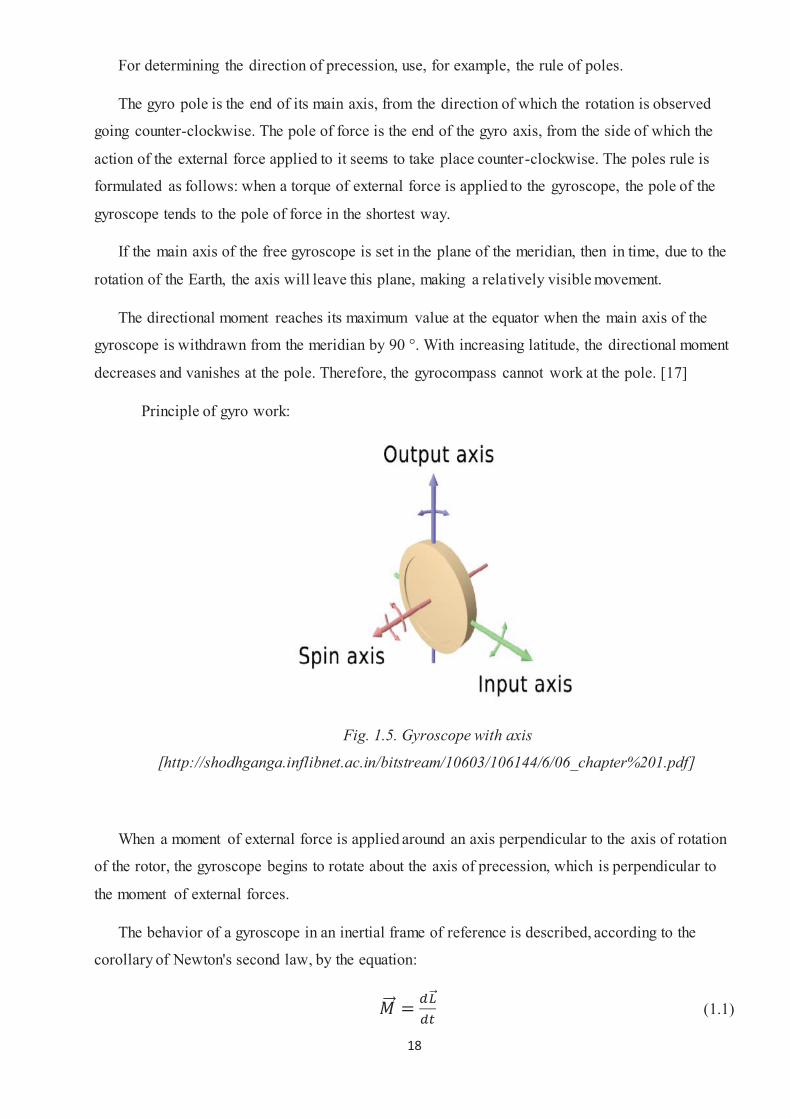
Principle of gyro work:

Fig. 1.5. Gyroscope with axis

[http://shodhganga.inflibnet.ac.in/bitstream/10603/106144/6/06_chapter%201.pdf]

When a moment of external force is applied around an axis perpendicular to the axis of rotation

of the rotor, the gyroscope begins to rotate about the axis of precession, which is perpendicular to

the moment of external forces.

The behavior of a gyroscope in an inertial frame of reference is described, according to the

corollary of Newton's second law, by the equation:

(1.1)

19

where the vectors and are, respectively, the moment of the force acting on the

gyroscope, and its angular momentum. [3]

The change in the angular momentum vector under the action of the moment of force is

possible not only in magnitude, but also in direction. In particular, the moment of force

applied perpendicular to the axis of rotation of the gyroscope, that is, perpendicular to , leads

to a motion perpendicular to both and , that is, to the phenomenon of precession. The

angular velocity of the precession of the gyroscope is determined by its angular momentum

and the moment of the applied force:

(1.2)

that is, is inversely proportional to the moment of the gyroscope rotor impulse, or, with

the rotor inertia moment unchanged, its rotation speed.

Simultaneously with the emergence of precession, according to the consequence of

Newton's third law, the gyroscope will act on the surrounding bodies by the moment of the

reaction, equal in magnitude and opposite in direction to the moment , applied to the

gyroscope. This reaction time is called the gyroscopic moment.

The same movement of the gyroscope can be interpreted differently if one uses a noninertial

reference frame connected with the rotor casing and introduces in it a fictitious inertia force, the

so-called Coriolis force. Thus, under the influence of the moment of external force, the

gyroscope will first rotate in the direction of the action of the external moment (nutational

throw). Each particle of the gyroscope will thus move with a portable angular velocity of

rotation due to the action of this moment. But the rotor of the gyroscope, in addition, itself

rotates, so each particle will have a relative speed. As a result, a Coriolis force arises that causes

the gyroscope to move in a direction perpendicular to the applied torque, that is, precession. [3]

20

Applications of north seeking gyros:

Gyro north finder is common directional instrument in this years, and pendulous gyroscope

has been widely used in the field of aviation, aerospace, detection, tunnels, military, etc. In

practical applications, such as missile without-relying fast launching, it needs that north -

seeking time is as short as possible under the premise of ensuring the accuracy. Therefore, it has

important application value how to achieve fast north seeking in a shorter swing process.

Application fields:

- Tunnel building

- Mining

- Topography

- Education at universities

- Military

21

1.3 Existing gyros

Sokkia X II

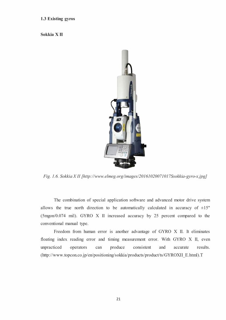
Fig. 1.6. Sokkia X II [http://www.elmeg.org/images/20161020071017Ssokkia-gyro-x.jpg]

The combination of special application software and advanced motor drive system

allows the true north direction to be automatically calculated in accuracy of ±15"

(5mgon/0.074 mil). GYRO X II increased accuracy by 25 percent compared to the

conventional manual type.

Freedom from human error is another advantage of GYRO X II. It eliminates

floating index reading error and timing measurement error. With GYRO X II, even

unpracticed operators can produce consistent and accurate results.

(http://www.topcon.co.jp/en/positioning/sokkia/products/product/ts/GYROXII_E.html).T

22

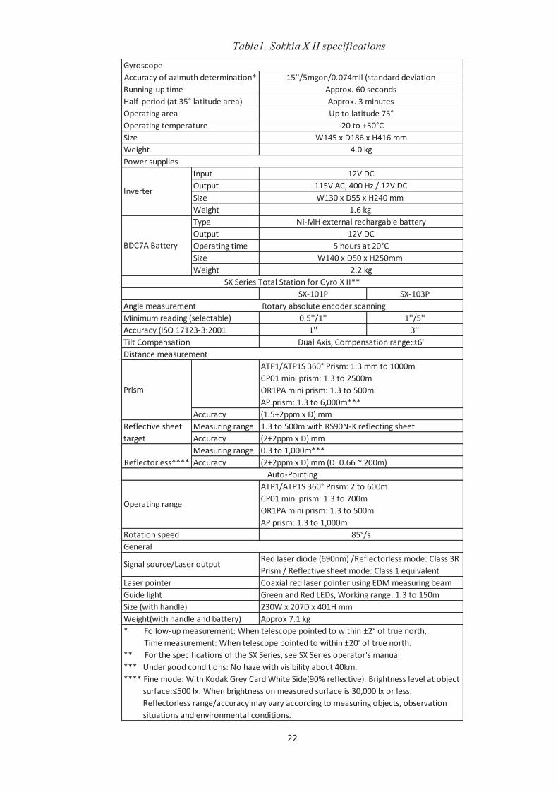
Table1. Sokkia X II specifications

InputOutputSizeWeightTypeOutputOperating timeSize Weight

SX-101P SX-103P

0.5''/1'' 1''/5''1'' 3''

AccuracyMeasuring rangeAccuracyMeasuring rangeAccuracy

* Follow-up measurement: When telescope pointed to within ±2° of true north, time Time measurement: When telescope pointed to within ±20' of true north. ** For the specifications of the SX Series, see SX Series operator's manual *** Under good conditions: No haze with visibility about 40km. **** Fine mode: With Kodak Grey Card White Side(90% reflective). Brightness level at object z surface:≤500 lx. When brightness on measured surface is 30,000 lx or less. z Reflectorless range/accuracy may vary according to measuring objects, observation z situations and environmental conditions.

Weight(with handle and battery)

Red laser diode (690nm) /Reflectorless mode: Class 3R Prism / Reflective sheet mode: Class 1 equivalentCoaxial red laser pointer using EDM measuring beamGreen and Red LEDs, Working range: 1.3 to 150m230W x 207D x 401H mmApprox 7.1 kg

General

Signal source/Laser output

Laser pointerGuide lightSize (with handle)

Auto-Pointing

Operating range

Rotation speed

ATP1/ATP1S 360° Prism: 2 to 600m CP01 mini prism: 1.3 to 700m OR1PA mini prism: 1.3 to 500m AP prism: 1.3 to 1,000m

85°/s

Reflective sheet target

Reflectorless****

1.3 to 500m with RS90N-K reflecting sheet(2+2ppm x D) mm0.3 to 1,000m***(2+2ppm x D) mm (D: 0.66 ~ 200m)

Tilt Compensation Dual Axis, Compensation range:±6'Distance measurement

Prism

ATP1/ATP1S 360° Prism: 1.3 mm to 1000m CP01 mini prism: 1.3 to 2500m OR1PA mini prism: 1.3 to 500m AP prism: 1.3 to 6,000m***(1.5+2ppm x D) mm

SX Series Total Station for Gyro X II**

Angle measurement Rotary absolute encoder scanningMinimum reading (selectable)Accuracy (ISO 17123-3:2001

BDC7A Battery

12V DC115V AC, 400 Hz / 12V DCW130 x D55 x H240 mm

1.6 kg Ni-MH external rechargable battery

12V DC5 hours at 20°C

W140 x D50 x H250mm 2.2 kg

Size W145 x D186 x H416 mm

Power supplies

Inverter

Operating areaOperating temperature

Approx. 3 minutesUp to latitude 75°

-20 to +50°C

Accuracy of azimuth determination* 15''/5mgon/0.074mil (standard deviationRunning-up time Approx. 60 secondsHalf-period (at 35° latitude area)

Gyroscope

Weight 4.0 kg

23

GTS-1 Automatic Gyroscope Total Station(BOIF)

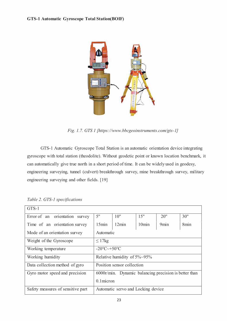
Fig. 1.7. GTS 1 [https://www.bbcgeoinstruments.com/gts-1]

GTS-1 Automatic Gyroscope Total Station is an automatic orientation device integrating

gyroscope with total station (theodolite). Without geodetic point or known location benchmark, it

can automatically give true north in a short period of time. It can be widely used in geodesy,

engineering surveying, tunnel (culvert) breakthrough survey, mine breakthrough survey, military

engineering surveying and other fields. [19]

Table 2. GTS-1 specifications

GTS-1

Error of an orientation survey 5'' 10'' 15'' 20'' 30''

Time of an orientation survey 15min 12min 10min 9min 8min

Mode of an orientation survey Automatic

Weight of the Gyroscope ≤ 17kg

Working temperature -20℃~+50℃

Working humidity Relative humidity of 5%~95%

Data collection method of gyro Position sensor collection

Gyro motor speed and precision 6000r/min. Dynamic balancing precision is better than

0.1micron

Safety measures of sensitive part Automatic servo and Locking device

24

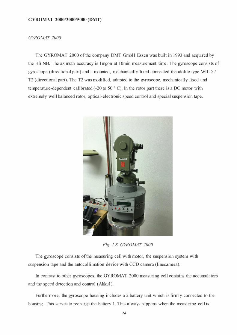
GYROMAT 2000/3000/5000 (DMT)

GYROMAT 2000

The GYROMAT 2000 of the company DMT GmbH Essen was built in 1993 and acquired by

the HS NB. The azimuth accuracy is 1mgon at 10min measurement time. The gyroscope consists of

gyroscope (directional part) and a mounted, mechanically fixed connected theodolite type WILD /

T2 (directional part). The T2 was modified, adapted to the gyroscope, mechanically fixed and

temperature-dependent calibrated (-20 to 50 ° C). In the rotor part there is a DC motor with

extremely well balanced rotor, optical-electronic speed control and special suspension tape.

Fig. 1.8. GYROMAT 2000

The gyroscope consists of the measuring cell with motor, the suspension system with

suspension tape and the autocollimation device with CCD camera (linecamera).

In contrast to other gyroscopes, the GYROMAT 2000 measuring cell contains the accumulators

and the speed detection and control (Akku1).

Furthermore, the gyroscope housing includes a 2 battery unit which is firmly connected to the

housing. This serves to recharge the battery 1. This always happens when the measuring cell is

25

locked. Here is also a big disadvantage of the system: the life of the battery is about 5 years. The

battery change requires a complete disassembly and thus high costs (about 25000 €).

Measuring principle:

The rotor is tied by the suspension above the center of gravity (suspension tape) heavy (rotary

pendulum). In contrast to his desire to maintain the orientation in space during the rotation of the

rotor (SPIN MODE), the gravity binding causes a torque. This depends on the width and depends

on the orientation to the meridian.

On the suspension tape, the gyroscope performs a weakly damped oscillation around the vertical

axis. This can be observed (visually, camera).

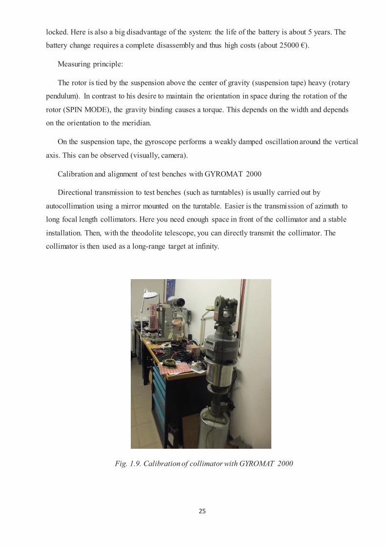
Calibration and alignment of test benches with GYROMAT 2000

Directional transmission to test benches (such as turntables) is usually carried out by

autocollimation using a mirror mounted on the turntable. Easier is the transmission of azimuth to

long focal length collimators. Here you need enough space in front of the collimator and a stable

installation. Then, with the theodolite telescope, you can directly transmit the collimator. The

collimator is then used as a long-range target at infinity.

Fig. 1.9. Calibration of collimator with GYROMAT 2000

26

GYROMAT 3000

The GYROMAT 3000 has accuracy of 1/1000th gon, which corresponds to a deviation in

arc of about 1.6 cm over a distance of one kilometer. The time needed for measuring a single

direction is about 10 minutes. This time can be reduced by applying two other survey programs

with reduced measuring accuracy. (https://www.dmt-group.com/products/geo-measuring-

systems/gyromat.html)

Table 3. GYROMAT 3000 specifications

Technical specifications

Measuring mods 1 2 3

Measuring accuracy in mgon * 1 10 5

Measuring time in minutes (approx.) 10 2 5

Measurements per battery charging 25 50 35

Operating temperature -20°C up to +50°C (-12°C up to +45°C calibrated)

Area of application Between 80° south latitude and 80° north latitude

Dimensions and weights

GYROMAT 5000(without theodolite) 11.5 kg, 215 mm centering diameter

Transport case Weight: 26 kg, (LxWxH) 460x460x800

Tripod Weight: 8 kg, 300 mm diameter

* Standard deviation (±1σ) under lab conditions in accordance with DIN 18723

27

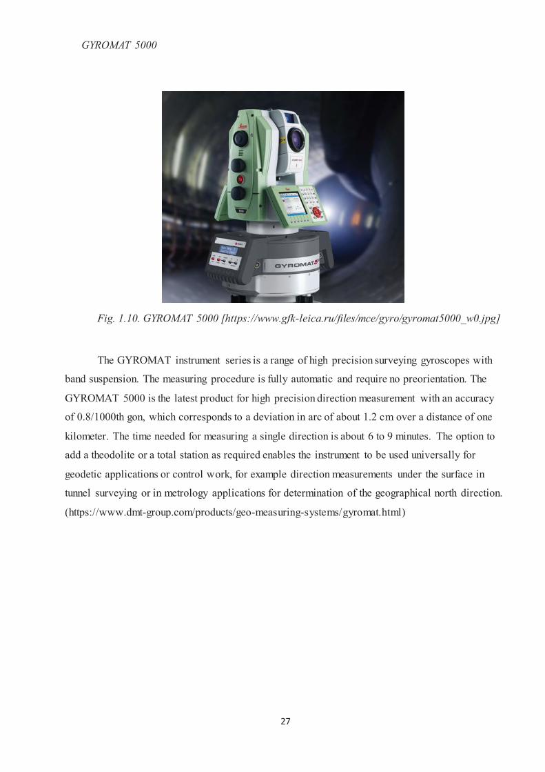
GYROMAT 5000

Fig. 1.10. GYROMAT 5000 [https://www.gfk-leica.ru/files/mce/gyro/gyromat5000_w0.jpg]

The GYROMAT instrument series is a range of high precision surveying gyroscopes with

band suspension. The measuring procedure is fully automatic and require no preorientation. The

GYROMAT 5000 is the latest product for high precision direction measurement with an accuracy

of 0.8/1000th gon, which corresponds to a deviation in arc of about 1.2 cm over a distance of one

kilometer. The time needed for measuring a single direction is about 6 to 9 minutes. The option to

add a theodolite or a total station as required enables the instrument to be used universally for

geodetic applications or control work, for example direction measurements under the surface in

tunnel surveying or in metrology applications for determination of the geographical north direction.

(https://www.dmt-group.com/products/geo-measuring-systems/gyromat.html)

28

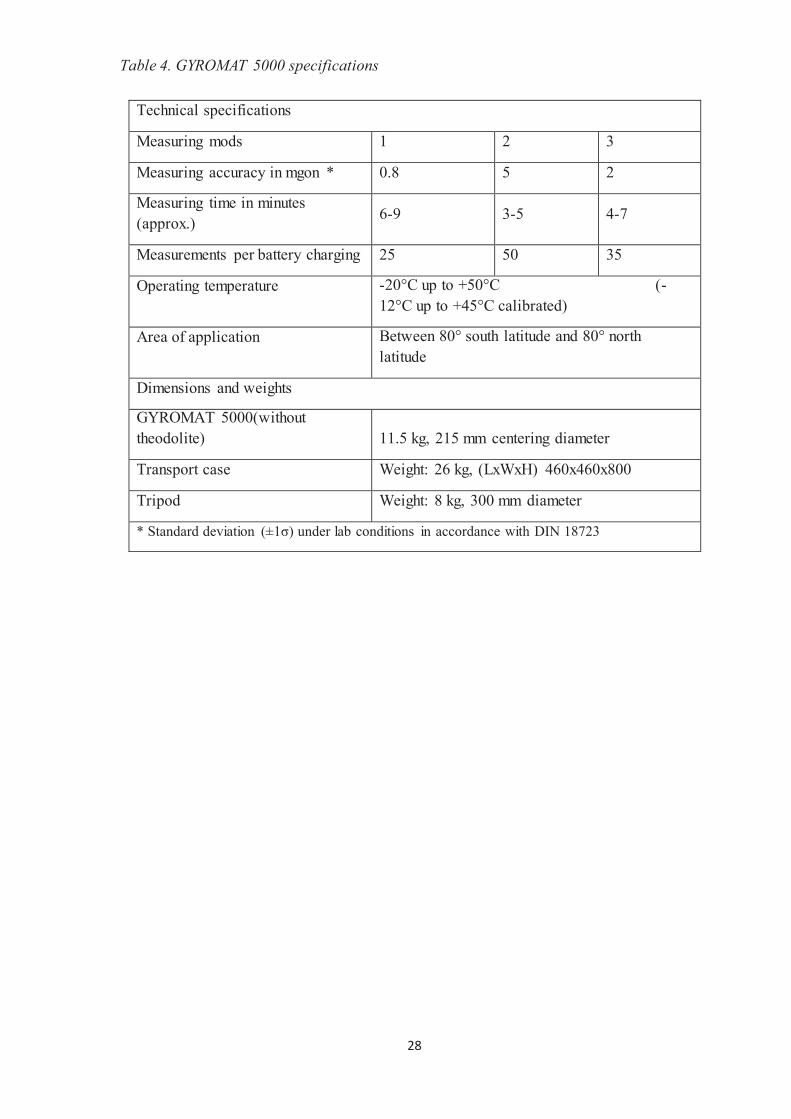
Table 4. GYROMAT 5000 specifications

Technical specifications

Measuring mods 1 2 3

Measuring accuracy in mgon * 0.8 5 2

Measuring time in minutes (approx.) 6-9 3-5 4-7

Measurements per battery charging 25 50 35

Operating temperature -20°C up to +50°C (-12°C up to +45°C calibrated)

Area of application Between 80° south latitude and 80° north latitude

Dimensions and weights

GYROMAT 5000(without theodolite) 11.5 kg, 215 mm centering diameter

Transport case Weight: 26 kg, (LxWxH) 460x460x800

Tripod Weight: 8 kg, 300 mm diameter

* Standard deviation (±1σ) under lab conditions in accordance with DIN 18723

29

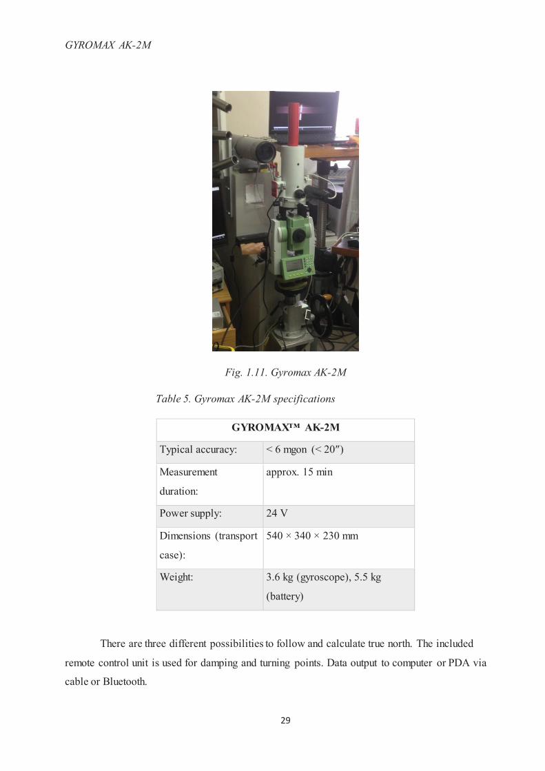
GYROMAX AK-2M

Fig. 1.11. Gyromax AK-2M

Table 5. Gyromax AK-2M specifications

GYROMAX™ AK-2M

Typical accuracy: < 6 mgon (< 20″)

Measurement

duration:

approx. 15 min

Power supply: 24 V

Dimensions (transport

case):

540 × 340 × 230 mm

Weight: 3.6 kg (gyroscope), 5.5 kg

(battery)

There are three different possibilities to follow and calculate true north. The included

remote control unit is used for damping and turning points. Data output to computer or PDA via

cable or Bluetooth.

30

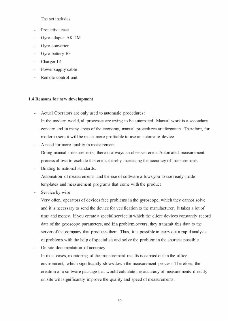
The set includes:

- Protective case

- Gyro adapter AK-2M

- Gyro converter

- Gyro battery B3

- Charger L4

- Power supply cable

- Remote control unit

1.4 Reasons for new development

- Actual Operators are only used to automatic procedures:

In the modern world, all processes are trying to be automated. Manual work is a secondary

concern and in many areas of the economy, manual procedures are forgotten. Therefore, for

modern users it will be much more profitable to use an automatic device

- A need for more quality in measurement

Doing manual measurements, there is always an observer error. Automated measurement

process allows to exclude this error, thereby increasing the accuracy of measurements

- Binding to national standards.

Automation of measurements and the use of software allows you to use ready-made

templates and measurement programs that come with the product

- Service by wire

Very often, operators of devices face problems in the gyroscope, which they cannot solve

and it is necessary to send the device for verification to the manufacturer. It takes a lot of

time and money. If you create a special service in which the client devices constantly record

data of the gyroscope parameters, and if a problem occurs, they transmit this data to the

server of the company that produces them. Thus, it is possible to carry out a rapid analysis

of problems with the help of specialists and solve the problem in the shortest possible

- On-site documentation of accuracy

In most cases, monitoring of the measurement results is carried out in the office

environment, which significantly slows down the measurement process. Therefore, the

creation of a software package that would calculate the accuracy of measurements directly

on site will significantly improve the quality and speed of measurements.

31

2. Methodology

2.1 Observation methods

According to [15], there are six methods of finding north using a suspended gyroscope. But

since this project is done for the Gyromax AK-2M model only the Pass-Through method is possible

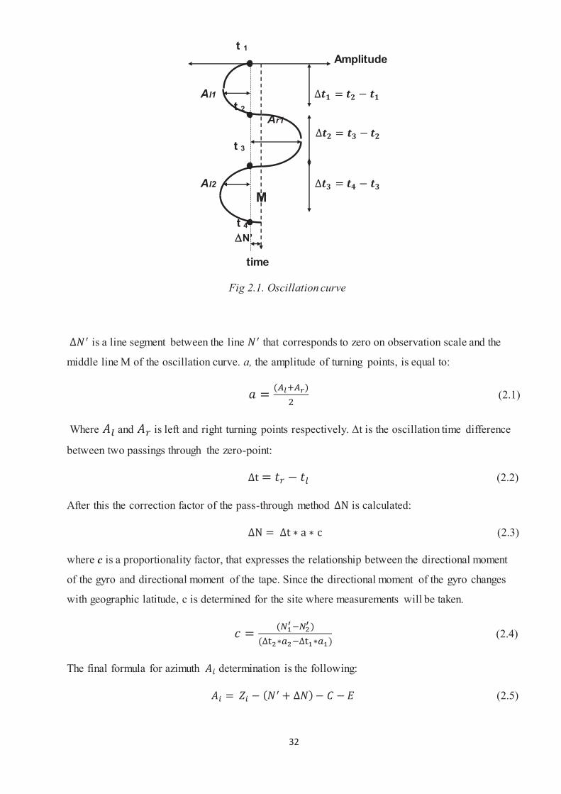
to perform with the line camera. Therefore, this method will be considered below. The oscillation

curve of the moving bar is shown in Fig. 2.1 as a function of time.

In this method, gyroscope has to be oriented to the north during the measurement process, that is

provided by pre-orientation procedure. Pre-orientation could be done by compass or by quick

defining of two turning points, one on the east from north, another on the west.

Before and after Pass Through measurement the tape-zero procedure has to be done. The

device should be turned off. With the released gyro, using the air brakes operator has to make the

light bar stay in the observation field. After damping the speed of light bar, operator records the

position of all turning points three times for each direction. After each procedure, aiming to the

target should be done twice.

The main measurement procedure is performed with the turned on gyro. After acceleration,

the gyro has to be released. The speed and position of the light bar can be regulated with air brakes.

As a rule, measurements are taken with the initial light bar moving from left to right. Each passing

of the light bar through the zero-point of the scale is marked with the timer. The positions of the

turning points are also recorded. After the measurement procedure gyro must be arrested and then

turned off.

32

t 1

Amplitude

Al1 t 2 Ar1 t 3 Al2 M t 4 N’ time Fig 2.1. Oscillation curve

is a line segment between the line that corresponds to zero on observation scale and the

middle line M of the oscillation curve. a, the amplitude of turning points, is equal to:

(2.1)

Where and is left and right turning points respectively. Δt is the oscillation time difference

between two passings through the zero-point:

(2.2)

After this the correction factor of the pass-through method is calculated:

(2.3)

where c is a proportionality factor, that expresses the relationship between the directional moment

of the gyro and directional moment of the tape. Since the directional moment of the gyro changes

with geographic latitude, с is determined for the site where measurements will be taken.

(2.4)

The final formula for azimuth determination is the following:

(2.5)

33

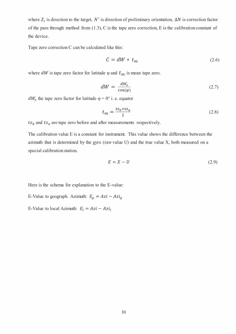
where is direction to the target, is direction of preliminary orientation, is correction factor

of the pass through method from (1.3), C is the tape zero correction, E is the calibration constant of

the device.

Tape zero correction C can be calculated like this:

(2.6)

where is tape zero factor for latitude φ and is mean tape zero.

(2.7)

the tape zero factor for latitude φ = 0° i. e. equator

(2.8)

and are tape zero before and after measurements respectively.

The calibration value E is a constant for instrument. This value shows the difference between the

azimuth that is determined by the gyro (raw value U) and the true value X, both measured on a

special calibration station.

(2.9)

Here is the schema for explanation to the E-value:

E-Value to geograph. Azimuth:

E-Value to local Azimuth:

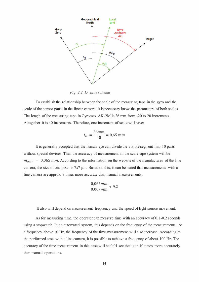
34

Fig. 2.2. E-value schema

To establish the relationship between the scale of the measuring tape in the gyro and the

scale of the sensor panel in the linear camera, it is necessary know the parameters of both scales.

The length of the measuring tape in Gyromax AK-2M is 26 mm from -20 to 20 increments.

Altogether it is 40 increments. Therefore, one increment of scale will have:

It is generally accepted that the human eye can divide the visible segment into 10 parts

without special devices. Then the accuracy of measurement in the scale tape system will be

. According to the information on the website of the manufacturer of the line

camera, the size of one pixel is 7x7 μm. Based on this, it can be stated that measurements with a

line camera are approx. 9 times more accurate than manual measurements:

It also will depend on measurement frequency and the speed of light source movement.

As for measuring time, the operator can measure time with an accuracy of 0.1-0.2 seconds

using a stopwatch. In an automated system, this depends on the frequency of the measurements. At

a frequency above 10 Hz, the frequency of the time measurement will also increase. According to

the performed tests with a line camera, it is possible to achieve a frequency of about 100 Hz. The

accuracy of the time measurement in this case will be 0.01 sec that is in 10 times more accurately

than manual operations.

35

2.2 Objectives

Nowadays, many types of gyroscopes require the user to read data manually, which can cause

the appearance of observer errors and increases the duration of measurements. If we consider

modern models of gyroscopes, in which there is the possibility of automatic measurements, then all

of them are in the highest price category and the purchase of which is beyond the means of many

companies. The main purpose of this work is the development of an automatic data reading system

with a gyro using a camera with a linear sensor with the ability to wirelessly transmit data. The cost

of developing of this system should not greatly affect on increasing in the cost of a gyro.

The main requirements for the system being developed are the following:

- The system must track the movement of the light strip and fix the position of the moment

when the strip changes direction or passes through the zero point of the scale.

- Compact size of the camera. The line camera must fit in the gyro housing and not interfere

with the operation of the remaining parts.

- Compactness of the control computer. The system should be small in size, which will facilitate

rapid transport and mobility measurements.

- Possibility of wireless data transmission

- The system should be easy to understand for an ordinary user. The number of operations

necessary to carry out measurements and transmit them must be minimized.

- Creation of a GUI on the receiving computer, which will output all necessary information

about the measurements and their processing.

2.3 Line camera

A linear photosensitive matrix is a semiconductor device that line-by-line converts the

optical image into an analog signal. There are two types of linear photosensitive matrices with

separate circuit configurations: CMOS and CCD matrices. Linear photosensitive matrices are

suitable for devices such as scan components for photocopiers, image and barcode scanners, single-

line scanning cameras used for visual studies (film, prints, textiles, etc.), grain sorters for color and

banknote recognition systems in bank terminals. [16]

36

Line scan applications

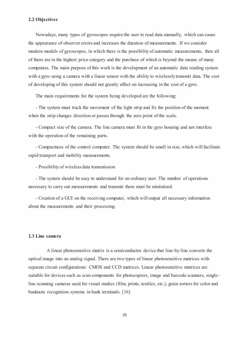
1) Web inspection

Line cameras are most effective when observing moving materials, in such industries as

paper production, printing, metallurgy, etc. Objects in such cases are immensely long and can be

accepted as infinitely long.

Fig. 2.3. Quality control of continuous product with line camera [https://www.stemmer-

imaging.com/media/cache/default_image_dialog/uploads/cameras/sis/gl/glossary-line-scan-

applications-1-en.JPG]

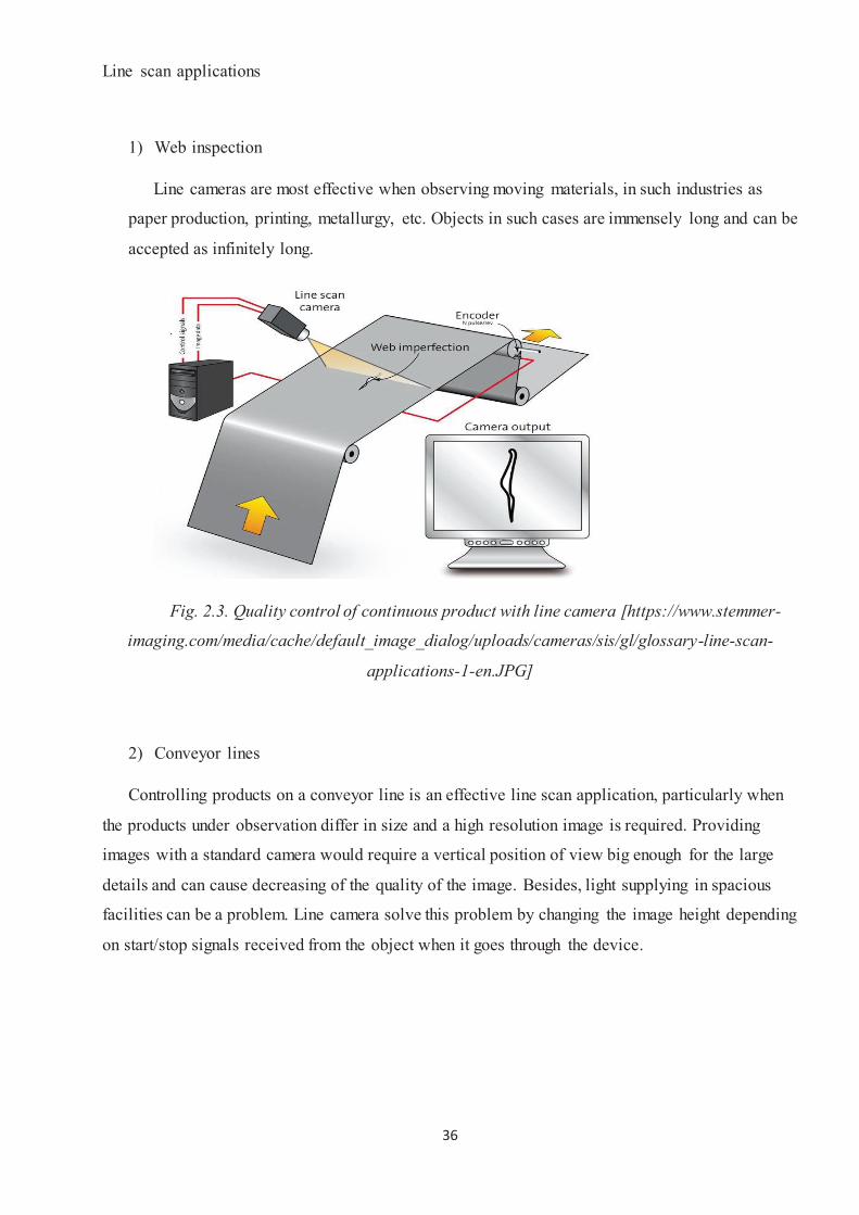
2) Conveyor lines

Controlling products on a conveyor line is an effective line scan application, particularly when

the products under observation differ in size and a high resolution image is required. Providing

images with a standard camera would require a vertical position of view big enough for the large

details and can cause decreasing of the quality of the image. Besides, light supplying in spacious

facilities can be a problem. Line camera solve this problem by changing the image height depending

on start/stop signals received from the object when it goes through the device.

37

Fig. 2.4. Inspection of objects on conveyor lines [https://www.stemmer-

imaging.com/media/cache/default_image_dialog/uploads/cameras/sis/gl/glossary-line-scan-

applications-2-en.JPG]

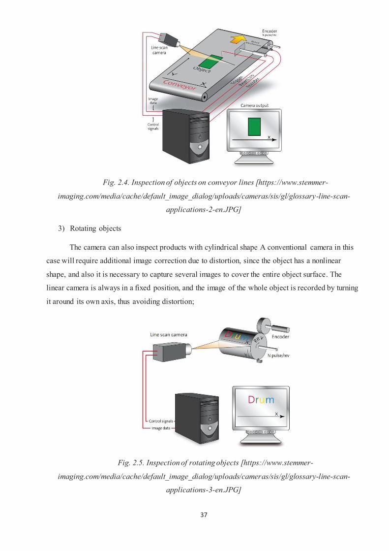
3) Rotating objects

The camera can also inspect products with cylindrical shape A conventional camera in this

case will require additional image correction due to distortion, since the object has a nonlinear

shape, and also it is necessary to capture several images to cover the entire object surface. The

linear camera is always in a fixed position, and the image of the whole object is recorded by turning

it around its own axis, thus avoiding distortion;

Fig. 2.5. Inspection of rotating objects [https://www.stemmer-

imaging.com/media/cache/default_image_dialog/uploads/cameras/sis/gl/glossary-line-scan-

applications-3-en.JPG]

38

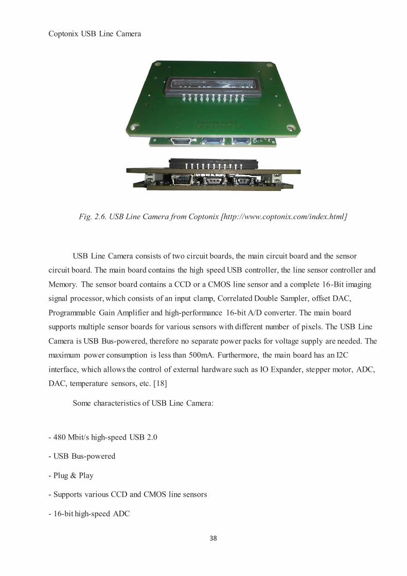
Coptonix USB Line Camera

Fig. 2.6. USB Line Camera from Coptonix [http://www.coptonix.com/index.html]

USB Line Camera consists of two circuit boards, the main circuit board and the sensor

circuit board. The main board contains the high speed USB controller, the line sensor controller and

Memory. The sensor board contains a CCD or a CMOS line sensor and a complete 16-Bit imaging

signal processor, which consists of an input clamp, Correlated Double Sampler, offset DAC,

Programmable Gain Amplifier and high-performance 16-bit A/D converter. The main board

supports multiple sensor boards for various sensors with different number of pixels. The USB Line

Camera is USB Bus-powered, therefore no separate power packs for voltage supply are needed. The

maximum power consumption is less than 500mA. Furthermore, the main board has an I2C

interface, which allows the control of external hardware such as IO Expander, stepper motor, ADC,

DAC, temperature sensors, etc. [18]

Some characteristics of USB Line Camera:

- 480 Mbit/s high-speed USB 2.0

- USB Bus-powered

- Plug & Play

- Supports various CCD and CMOS line sensors

- 16-bit high-speed ADC

39

- Correlated Double Sampler (CDS)

- 1~6x Programmable Gain, 64 increments

- ±300 mV Programmable Offset, 512 increments

- 2 programmable internal reference voltage 2V and 4V

- Trigger input

- 100kHz I2C-Master Interface

- Compact design 66 x 48 x 7.7 mm³ (without sensor)

- Integration time and frame rates are CCD/CMOS line sensor specific. [18]

The camera used for this job has a CMOS line sensor S12706 from the Hamamatsu company.

Table 6. Characteristics of the Hamamatsu sensor S12706

Sensor Type CMOS

Active pixel 4096

Pixel size [μm] 7 x 7

Min. Integration time [μs] 27

Sensivity [V/lx .s] 23

Dynamic Range 10000

Wavelength range [nm] 400-1000

Max. frame rate 440

The most important from the characteristics of sensor S12706 (Table 6) is CMOS

(complementary metal-oxide semiconductor) sensor type. In most CMOS devices, there are

several transistors at each pixel that amplify and move the charge using more traditional wires. The

CMOS approach is very flexible because each pixel can be read individually.

CMOS chips use traditional manufacturing processes to create the chip - the same processes

used to make most microprocessors. CMOS sensors, are more susceptible to noise, that other

sensors (e.g. CCD). Because each pixel on this sensor has several transistors located next to it, the

light sensitivity of a CMOS chip tends to be lower. Many of the photons hitting the chip hit the

40

transistors instead of the photodiode. CMOS traditionally consumes little power. Implementing a

sensor in CMOS yields a low-power sensor. [4]

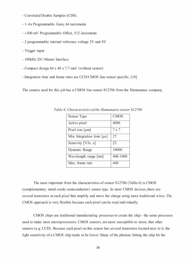
There are some important properties described in the manual for Hamamatsu sensor

S12706. For example, the spectral response at temperature 25 °С (Fig. 2.6).

The biggest value for relative sensitivity is in 625 nm wavelengths. This value is a

start point for the red spectral (620-750 wavelengths). Therefore, it is recommended to use a red

laser to improve the work of S12706 sensor.

Fig. 2.7. Spectral response for Hamamatsu sensor S12706

[https://www.coptonix.com/files/s12706_kmpd1146e.pdf]

2.4 Control computer

To perform automatic reading of gyro measurements, a man need a computer that meets the

following requirements:

1) The size of the computer board is quite compact, in order to adhere to the mobility and

speed of manipulations related to the connection of devices.

2) The cost of the device should not be high, since it is planned to supply gyroscopes with

computers.

3) The performance of the computer should be sufficient for a continuous and uninterrupted

process of data transmission and processing.

41

4) Support for a programming language that could provide communication with a line

camera, as well as carry out all necessary operations for processing and transmitting

received data.

5) Possibility of wireless data transmission.

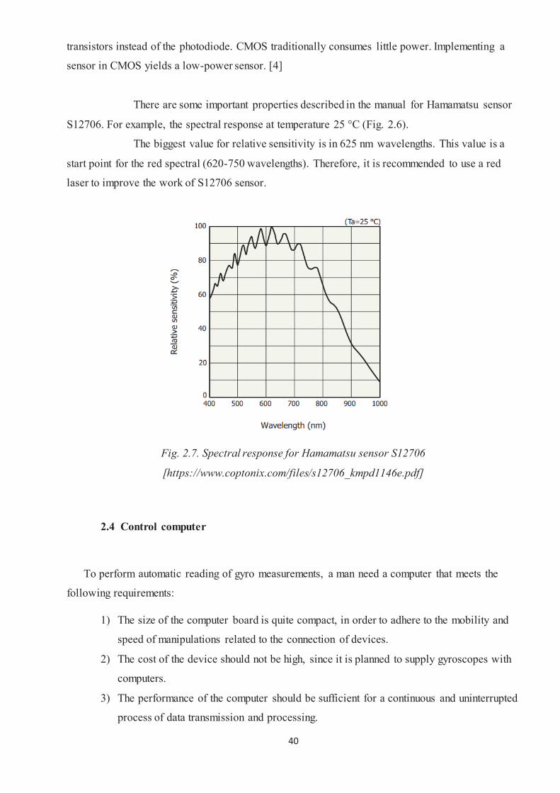
Based on the above requirements, a computer model Raspberry Pi 3B was chosen for this

research, and it fully meets these requirements. It is possible to connect a line camera to a computer

using a USB interface. Also there is an operating system with a graphical interface on the computer,

on which it is convenient to create the necessary programming code. It is a single-board computer

with wireless LAN and Bluetooth connections.

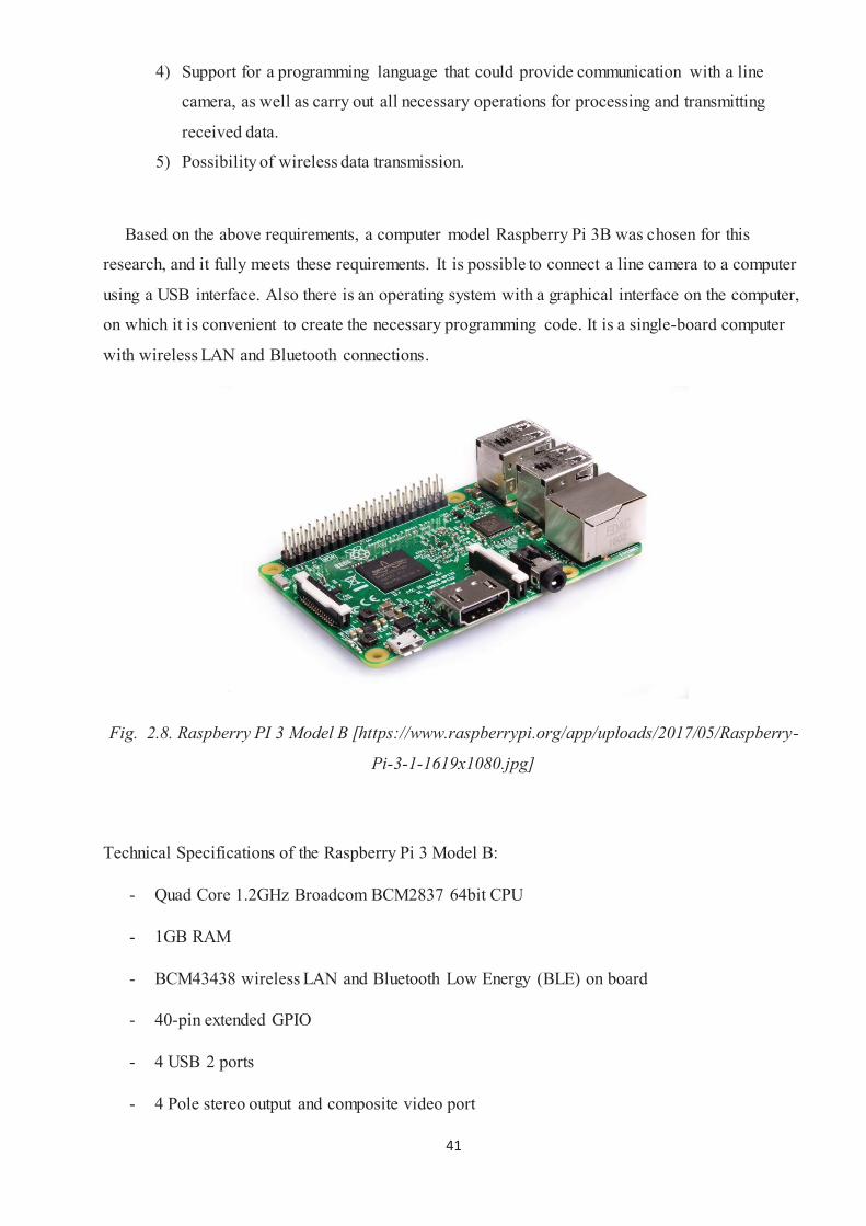
Fig. 2.8. Raspberry PI 3 Model B [https://www.raspberrypi.org/app/uploads/2017/05/Raspberry-

Pi-3-1-1619x1080.jpg]

Technical Specifications of the Raspberry Pi 3 Model B:

- Quad Core 1.2GHz Broadcom BCM2837 64bit CPU

- 1GB RAM

- BCM43438 wireless LAN and Bluetooth Low Energy (BLE) on board

- 40-pin extended GPIO

- 4 USB 2 ports

- 4 Pole stereo output and composite video port

42

- Full size HDMI

- CSI camera port for connecting a Raspberry Pi camera

- DSI display port for connecting a Raspberry Pi touchscreen display

- Micro SD port for loading your operating system and storing data

- Upgraded switched Micro USB power source up to 2.5A

2.5 Programming language

All programs and scripts were written in the Python 3 programming environment. This is a

high-level object-oriented programming language. High-level programming languages are designed

for the speed and convenience of using the programmer. The main feature of high-level languages is

abstraction, that is, the introduction of semantic constructions, which briefly describe such data

structures and operations on them, whose description on the machine code (or other low-level

programming language) is very long and difficult to understand. Object-oriented programming is

based on the presentation of the program in the form of a set of objects, each of which is an instance

of a certain class, and classes form an hierarchy of imitation. Also, one of the features of this

language is the support for dynamic typing, that is, the type of variable is determined only when

code execution.

Among the main advantages of Python should be:

• clean syntax (you must use indents to select blocks)

• portability of programs

• The standard distribution has a large number of useful modules

• The ability to use Python in dialog mode (useful function for experimenting and solving

simple tasks)

• convenient for solving mathematical problems (has tools for working with complex numbers,

can operate with integer numbers of arbitrary value, can be used as a powerful calculator in dialog

mode)

• open source (the ability to edit it by other users)

The tasks laid out in the programs are as follows:

• retrieving the data from line camera

43

• storing the data on web-service

• downloading the data from web-service

• detecting the pixels with highest light intensity

• finding the pixel, on which light changes its moving direction

• recording the timestamps of all measurements

• calculating all necessary values for azimuth computation

44

3. Implementation

3.1 Workflow

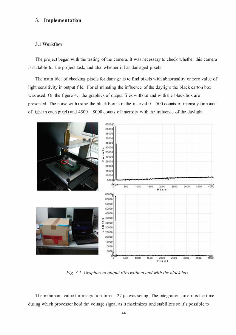
The project began with the testing of the camera. It was necessary to check whether this camera

is suitable for the project task, and also whether it has damaged pixels

The main idea of checking pixels for damage is to find pixels with abnormality or zero value of

light sensitivity in output file. For eliminating the influence of the daylight the black carton box

was used. On the figure 4.1 the graphics of output files without and with the black box are

presented. The noise with using the black box is in the interval 0 – 500 counts of intensity (amount

of light in each pixel) and 4500 – 8000 counts of intensity with the influence of the daylight.

Fig. 3.1. Graphics of output files without and with the black box

The minimum value for integration time – 27 μs was set up. The integration time it is the time

during which processor hold the voltage signal as it maximizes and stabilizes so it’s possible to

45

measure it. At the end of the integration time, processor “resets” the voltage back down to zero so

the sensor is ready for the next pulse.

With the black box the difference between maximum and minimum noise for every pixel was

on the average 200-300 counts of intensity (for 100 measurements in different time moments). The

value of counts of intensity varies from 0 to 65535 units, so the value 229 is only 0.35 %. Every

pixel had non zero value for 100 measurements. So there are no damage pixels. Because of each

pixel on a CMOS sensor has several transistors located next to it, every of 4096 pixels cannot has

the same characteristics. Many of the photons that hitting the chip, hit the transistors instead of the

photodiode.

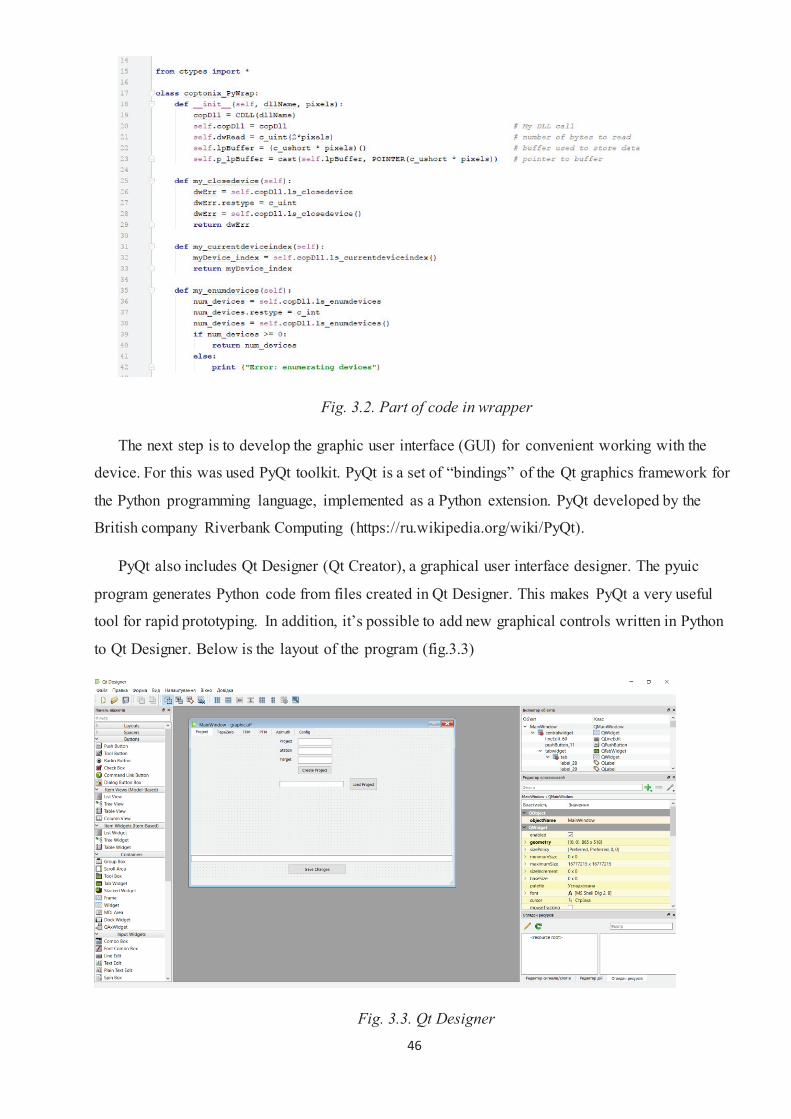
For this project were used programming language Python 3 and a part of code on C language,

which was written by camera producer. The important thing was to provide access to line-camera

using python code. Interaction with the camera is carried out using certain functions that are in a

special library file. Library is a collection of subroutines or classes used to develop software.

Libraries expose interfaces which clients of the library use to execute library routines

(https://en.wikipedia.org/wiki/Wrapper_library). But since there was only the library for C-

languages, a wrapper library was created. Wrapper libraries consist of a thin layer of code which

translates a library’s existing interface into a compatible interface. There is a foreign function

library in Python which allows to use C compatible data types and gives a possibility to call

functions in DLLs or shared libraries.

The class which has been used is a wrapper that allows the user to call the usblc32.dll Delphi

library from a Python code. All parameters passed into functions and classes in this module can be

regular pythonic types, and all return values are pythonic types as well. All type conversions are

carried out within the wrapper, for which the 'ctypes' module is internally used.

46

Fig. 3.2. Part of code in wrapper

The next step is to develop the graphic user interface (GUI) for convenient working with the

device. For this was used PyQt toolkit. PyQt is a set of “bindings” of the Qt graphics framework for

the Python programming language, implemented as a Python extension. PyQt developed by the

British company Riverbank Computing (https://ru.wikipedia.org/wiki/PyQt).

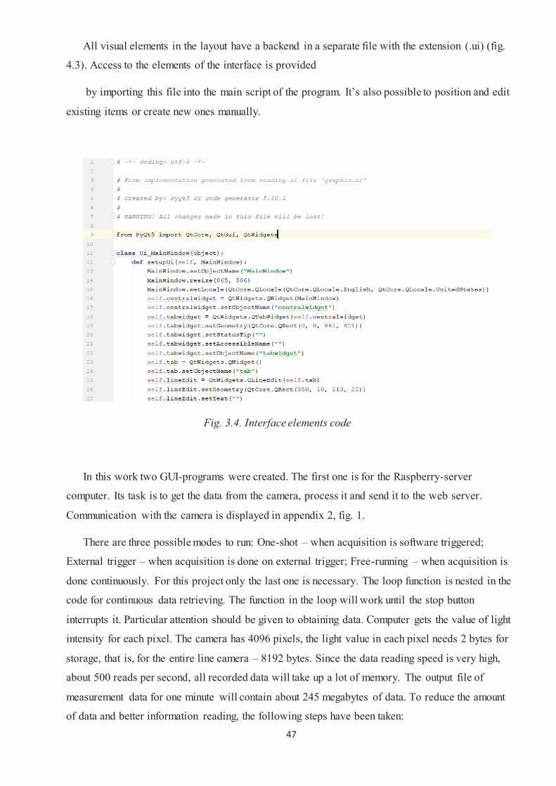
PyQt also includes Qt Designer (Qt Creator), a graphical user interface designer. The pyuic

program generates Python code from files created in Qt Designer. This makes PyQt a very useful

tool for rapid prototyping. In addition, it’s possible to add new graphical controls written in Python

to Qt Designer. Below is the layout of the program (fig.3.3)

Fig. 3.3. Qt Designer

47

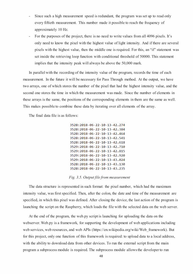
All visual elements in the layout have a backend in a separate file with the extension (.ui) (fig.

4.3). Access to the elements of the interface is provided

by importing this file into the main script of the program. It’s also possible to position and edit

existing items or create new ones manually.

Fig. 3.4. Interface elements code

In this work two GUI-programs were created. The first one is for the Raspberry-server

computer. Its task is to get the data from the camera, process it and send it to the web server.

Communication with the camera is displayed in appendix 2, fig. 1.

There are three possible modes to run: One-shot – when acquisition is software triggered;

External trigger – when acquisition is done on external trigger; Free-running – when acquisition is

done continuously. For this project only the last one is necessary. The loop function is nested in the

code for continuous data retrieving. The function in the loop will work until the stop button

interrupts it. Particular attention should be given to obtaining data. Computer gets the value of light

intensity for each pixel. The camera has 4096 pixels, the light value in each pixel needs 2 bytes for

storage, that is, for the entire line camera – 8192 bytes. Since the data reading speed is very high,

about 500 reads per second, all recorded data will take up a lot of memory. The output file of

measurement data for one minute will contain about 245 megabytes of data. To reduce the amount

of data and better information reading, the following steps have been taken:

48

- Since such a high measurement speed is redundant, the program was set up to read only

every fiftieth measurement. This number made it possible to reach the frequency of

approximately 10 Hz.

- For the purposes of the project, there is no need to write values from all 4096 pixels. It’s

only need to know the pixel with the highest value of light intensity. And if there are several

pixels with the highest value, then the middle one is required. For this, an “if” statement was

set inside the retrieving loop function with conditional threshold of 50000. This statement

implies that the intensity peak will always be above the 50,000 mark.

In parallel with the recording of the intensity value of the program, records the time of each

measurement. In the future it will be necessary for Pass Through method. At the output, we have

two arrays, one of which stores the number of the pixel that had the highest intensity value, and the

second one stores the time in which the measurement was made. Since the number of elements in

these arrays is the same, the positions of the corresponding elements in them are the same as well.

This makes possible to combine these data by iterating over all elements of the array.

The final data file is as follows:

Fig. 3.5. Output file from measurement

The data structure is represented in such format: the pixel number, which had the maximum

intensity value, was first specified. Then, after the colon, the date and time of the measurement are

specified, in which this pixel was defined. After closing the device, the last action of the program is

launching the script on the Raspberry, which loads the file with the selected data on the web server.

At the end of the program, the web.py script is launching for uploading the data on the

webserver. Web.py is a framework, for supporting the development of web applications including

web services, web resources, and web APIs (https://en.wikipedia.org/wiki/Web_framework). But

for this project, only one function of this framework is required: to upload data to a local address,

with the ability to download data from other devices. To run the external script from the main

program a subprocess module is required. The subprocess module allows the developer to run

49

program processes from Python. In other words, it’s possible to run applications and pass arguments

to them using the subprocess module.

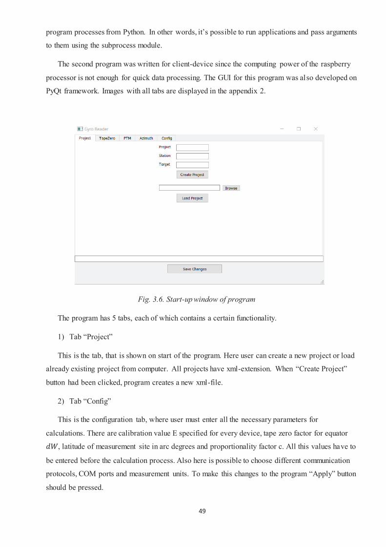
The second program was written for client-device since the computing power of the raspberry

processor is not enough for quick data processing. The GUI for this program was also developed on

PyQt framework. Images with all tabs are displayed in the appendix 2.

Fig. 3.6. Start-up window of program

The program has 5 tabs, each of which contains a certain functionality.

1) Tab “Project”

This is the tab, that is shown on start of the program. Here user can create a new project or load

already existing project from computer. All projects have xml-extension. When “Create Project”

button had been clicked, program creates a new xml-file.

2) Tab “Config”

This is the configuration tab, where user must enter all the necessary parameters for

calculations. There are calibration value E specified for every device, tape zero factor for equator

, latitude of measurement site in arc degrees and proportionality factor c. All this values have to

be entered before the calculation process. Also here is possible to choose different communication

protocols, COM ports and measurement units. To make this changes to the program “Apply” button

should be pressed.

50

3) Tab “Tape Zero”

Here user can calculate the tape zero before and after the measurement. The direction to the

target has to be entered here as well. User can switch between radio buttons “Before measure” and

“After measure” for the relevant procedures. There are three buttons. The “Download the data” is

responsible for downloading the data from web-server and storing it in text file. The “Compute”

button performs all necessary calculations to obtain tape zero. The flowchart with computation

algorithm of tape zero is displayed in appendix 1, fig 3. The “Z Measure” button sets the relevant

value equal to the value, that was entered in the field.

4) Tab “PTM”

All calculations of pass through method are done here. First, user has to download the data with

the self-titled button. This procedure is the same as in “Tape zero” tab. It is necessary to set

preliminary orientation angle before further calculations. In the upper-left corner of tab, there is a

field and self-titled button for this. The “Computation” button is responsible for calculations of the

pass through method. The flowchart with PTM computation algorithm is displayed in appendix 1,

fig 4. After pressing this button several values are displayed on the screen: the time of each passing

of light bar through zero-point of measuring scale, turning points, average value of correction

factors of the pass-through method and standard deviation of this value.

5) Tab “Azimuth”

This tab is for displaying the results of measurement and stores all necessary values. Here user

can see values of each element that was used in calculation.

After processing procedure user can save results of the measurement in the xml-file. The structure

of xml-file is displayed in appendix 3.

Algorithm of computation

The next step is to describe the process of detection of the turning points and zero-crossings.

First of all, program has to download data file from the web server, recognize the data structure and

extract all necessary information. For this, client computer has to know IP-address of raspberry

device. After this, program reads the data from web-server, decodes this text into UTF-8 format

(Unicode Transformation Format, 8 bit) and writes it to the text file on the running computer.

When the data file already stored on the client computer, it’s possible to start computation

process. The computation goes in the following order:

51

1) Tape zero before

2) Pass through method

3) Tape zero after

The first and the third procedures are the same, except the file, they are using. For each type of

measurement exists the different text files – for tape zero before, pass through and tape zero after.

The pass through computation procedure is similar to other two, but has additional zero-crossing

detection function.

After initialization of computation process, program call function named “extraction”. Here it

opens text file with the relevant data. The function iterates trough each line in file and appends them

to new array variable in string data type. If there’s some empty lines in the file, program skips it.

After this, the function splits each element in array on two new and appends each of them into the

separate arrays. The program separates data using special sign “ : ”. Everything that is before this

sign goes to one array, and the rest part after this sign to another. Also it’s necessary to transform

the time format to float type for further computations. This task is carried out by “gettime” sub-

function. It transforms hours, minutes, seconds into the seconds format with floating point. In the

end, “extraction” function returns either pixel or timestamp array depending on purpose.

Since the moving of light in real conditions will not be linear, it’s necessary to filter the pixel

consequence that represents the moving of light. For this a several filters were used. First filter

function detects if the neighboring pixels have the same value, and if filter finds it, one of the

elements will be removed from array as well as its time stamp. Second filter function detects

inconsistent elements in pixel array. The program checks every pixel and its left and right neighbor.

There are two cases of “invalid” pixels: if this pixel number is less than its two neighbors or on the

contrary – when the pixel number is greater. For example:

234, 235, 237, 239, 242, 240, 245, 246, 248, 250

387, 385, 382, 381, 379, 381, 379, 378, 376, 373

When array is filtered and has a smooth consequence it is ready for turning point detection.

The function “null_ones” converts the array of pixel numbers into array of “0” and “1”. If the

previous element of array is greater than the next one, function appends value “0” to the new array.

In case when the previous element is less than the next one, function appends value “1”. As a result,

we have a new array that looks like this:

…000000000011111…11111100000…0000001111…11111

52

Every element of this array corresponds to the pixel number in the pixel array. The final task

reduces to find the position of an element, that is not equal to the previous one. This is done by

“turning_points” function. The position of this element corresponds to the turning pixel. The

function appends to the new array only those pixels that are turning points. And the final task is to

return this pixel positions as a dictionary that has such keys as: “left1”, “right1”, “left2”, “right2”,

“left3” and “right3”, which correspond to consequence of tape zero turning points.

This algorithm also works for pass through method for finding turning pixels. The feature of

this method is that it is necessary to determine the time of crossing the middle pixel of the line

camera (that is 2048) by the light beam. There is a several possibilities how this time could be

detected. Since the size of the pixels is very small and the moving speed the light beam is relatively

high, the position of the light in the next moment could be located not in the next pixel. For

example:

2040, 2041, 2043, 2045, 2047, 2049, 2051, 2053, 2054

As you can see, there is no 2048 pixel. But the solution is to interpolate the neighboring

elements using the following condition: if the previous element is less than 2048 and the next

element is greater than 2048 then the time stamps of this pixels added together and divided by their

sum, i.e. by 2.

The other possibility is when there is one or more pixels with 2048 value. Then program

counts the amount of this pixels and finds the average time.

2040, 2041, 2043, 2045, 2048, 2048, 2051, 2053, 2054

The remaining calculations are made according to the formulas from the Section 2.

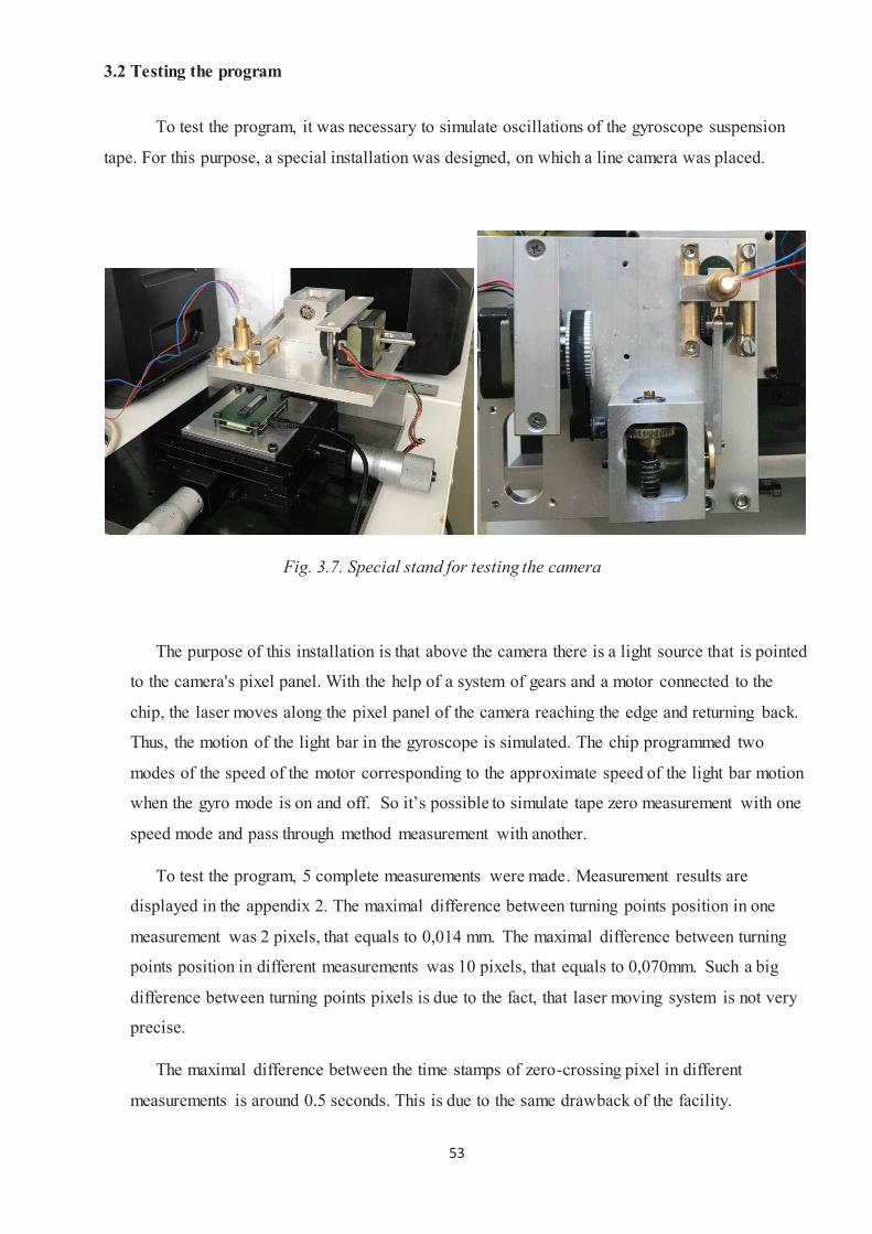
53

3.2 Testing the program

To test the program, it was necessary to simulate oscillations of the gyroscope suspension

tape. For this purpose, a special installation was designed, on which a line camera was placed.

Fig. 3.7. Special stand for testing the camera

The purpose of this installation is that above the camera there is a light source that is pointed

to the camera's pixel panel. With the help of a system of gears and a motor connected to the

chip, the laser moves along the pixel panel of the camera reaching the edge and returning back.

Thus, the motion of the light bar in the gyroscope is simulated. The chip programmed two

modes of the speed of the motor corresponding to the approximate speed of the light bar motion

when the gyro mode is on and off. So it’s possible to simulate tape zero measurement with one

speed mode and pass through method measurement with another.

To test the program, 5 complete measurements were made. Measurement results are

displayed in the appendix 2. The maximal difference between turning points position in one

measurement was 2 pixels, that equals to 0,014 mm. The maximal difference between turning

points position in different measurements was 10 pixels, that equals to 0,070mm. Such a big

difference between turning points pixels is due to the fact, that laser moving system is not very

precise.

The maximal difference between the time stamps of zero-crossing pixel in different

measurements is around 0.5 seconds. This is due to the same drawback of the facility.

54

Conclusions

During this investigation, the following was done:

1) Several Gyromax AK-2M gyros were calibrated on calibration stand for understanding the

features of the measurement process in non-automatized device. The calibration procedure included

a TPM measurement at five different tape-zero positions (0, +4, +8, -4, -8) and PTM measurement

to determine a c-value.

2) A GYROMAT 2000 gyro was used to check the azimuth of 2 collimators that are used for gyro

E-Value calibration.

3) A linear camera from Coptonix has been tested for use in Gyromax AK-2M gyros. The camera

pixels interpret the light that enters them as quantity units from 0 to 65535. Testing showed that the

camera is working properly, no damaged pixels were detected. Camera parameters meet project

requirements.

4) Software has been created for communicating with the camera, processing the data received from

it, and calculating the necessary values. Python programming language was used for this task. The

software is represented by two programs with a graphical interface. One of them developed on the

single-board computer Raspberry 3B and responsible for data acquisition, the other on the client

computer, that processes the data and makes computations. The software has user-friendly graphic

user interface which allows user to make all necessary operations. The end result of the program is

the xml-file with the results of measurements. Results of the measurements are indicated in the

appendix 3

5) A special installation for the simulation of gyro oscillation was created. Reproduction of the

oscillation process is carried out by means of a moving light source driven by a system of gears

connected to the motor. System has two speed modes for different measurement methods. It can be

used in further research.

The accuracy of measurements in automatic mode will depend on the frequency of the

measurements and the size of the pixels. If for manual measurements the accuracy of the amplitude

determination is around 0.1-0.2 scale increments, then for automatic measurement this value should

be less than 0.1 scale increment. For manual measurement of time accuracy is around 0.1-0.2 sec.,

so for automatic mode it supposed to be less than 0.1 sec., i. e. frequency of measurement should be

greater than 10 Hz. In practice, it’s possible to reach 100 Hz frequency. Summarizing all of the

above, it can be stated that the accuracy of the automatic measurement is 10 times higher than the

55

manual accuracy. It should also be noted that in automatic measurements, an observer error is

excluded. To implement this project for the AK-2M gyro, it is necessary to design a suitable size of

the line camera shape for installation in the housing of device.

56

References

[1] L. Foucault. Démonstration physique du mouvement de rotation de la terre au moyen du

pendula. C. r. hebd. séances Acad. sci. Paris, 32 (1851), pp. 135-138

[2] В. Ковтун, В. Хегер, И. Тревого, Л. Чаплинская // Геопрофиль. – 2010. – № 4. – С. 34–40

[3] Гироскоп.

https://ru.wikipedia.org/wiki/%D0%93%D0%B8%D1%80%D0%BE%D1%81%D0%BA%D0%BE

%D0%BF

[4] What is the difference between CCD and CMOS image sensors in a digital camera?

https://electronics.howstuffworks.com/cameras-photography/digital/question362.html

[5] Introduction. http://shodhganga.inflibnet.ac.in/bitstream/10603/106144/6/06_chapter%201.pdf

[6] WF Caspary - Applied Geodesy, 1987 – Springer

[7] Johann G. F. Bohnenberger «Beschreibung einer Maschine zur Erläuterung der Gesetze der

Umdrehung der Erde um ihre Axe, und der Veränderung der Lage der letzteren». 1817

[8] Шестов С. А «Гироскоп на земле, в небесах и на море.» – М: Знание, 1989 – С. 70

[9] "Elmer Sperry Dies. Famous Inventor". New York Times. June 17, 1930

[10] Голованов В.А. Гироскопическое ориентирование: Учеб. пособие / В.А. Голованов.

Санкт-Петербургский государственный горный институт. СПб, 2004. 92 с.

[11] Kreiselprobleme / Gyrodynamics: Symposion Celerina, 20. Bis 23. August 1962

[12] Воронков Н.Н. Гироскопическое ориентирование / Н.Н.Воронков, В.В.Кутырев,

Н.М.Ашимов. 2-е изд., перераб. и доп. М.: Недра, 1980. 296 с.

[13] Hendrik C. I. Grobler. Azimuth determination by gyroscope, 50 years later, has anything

changed? 16th international congress for mine surveying, Brisbane, Australia, 12-16 Sept 2016

[14] GPX Gyro Station. https://www.sokkia.com.sg/products/gyro/uploads/GPxX_Brochure.pdf

[15] Thomas, T.L.: The Six Methods of Finding North Using a Suspended Gyroscope.

Survey Review (26), pp. 225-235, 1982.

[16] Linear Image Sensors https://toshiba.semicon-storage.com/eu/product/sensor/linear-

sensor.html

[17] Gyroscope http://ed-thelen.org/Gyro-hcmut.html

57

[18] Coptonix Line camera https://www.coptonix.com/_en/html/usblinecamera.html

[19] GTS-1 https://www.bbcgeoinstruments.com/gts-1

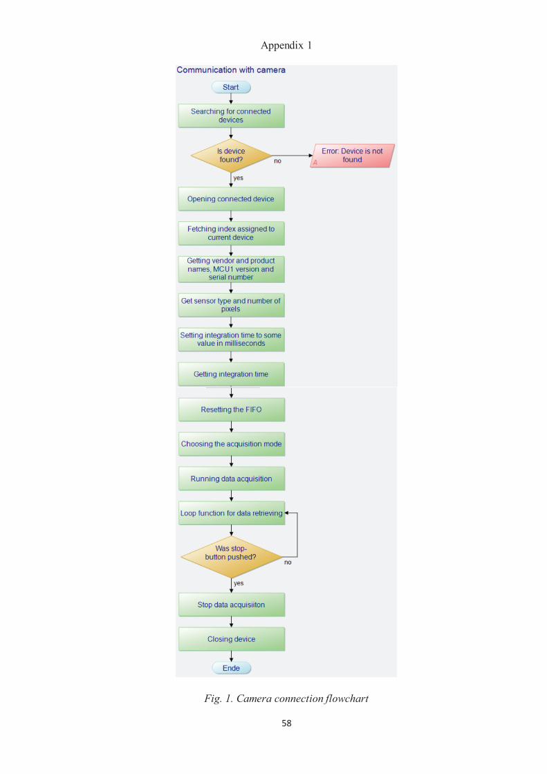
58

Appendix 1

Fig. 1. Camera connection flowchart

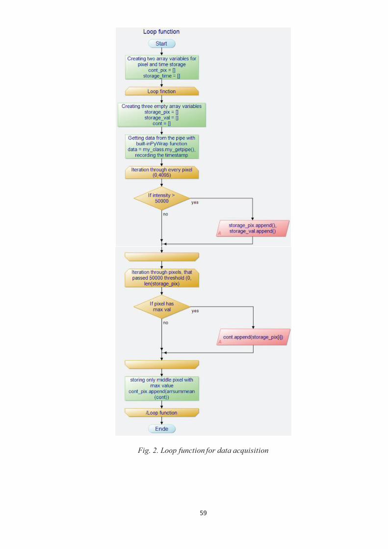
59

Fig. 2. Loop function for data acquisition

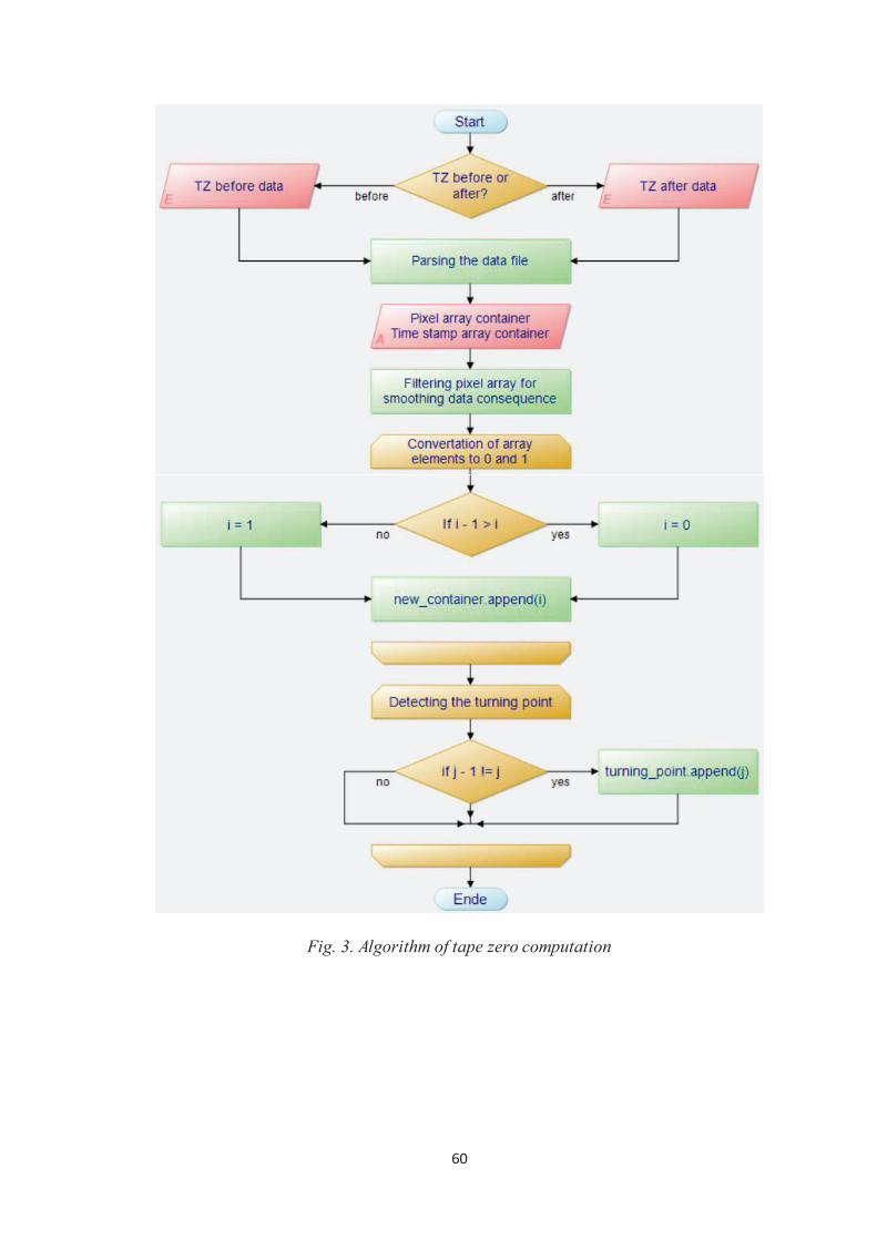
60

Fig. 3. Algorithm of tape zero computation

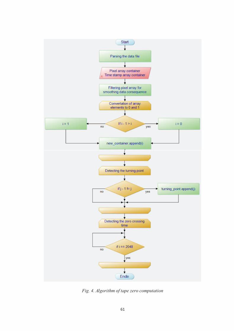
61

Fig. 4. Algorithm of tape zero computation

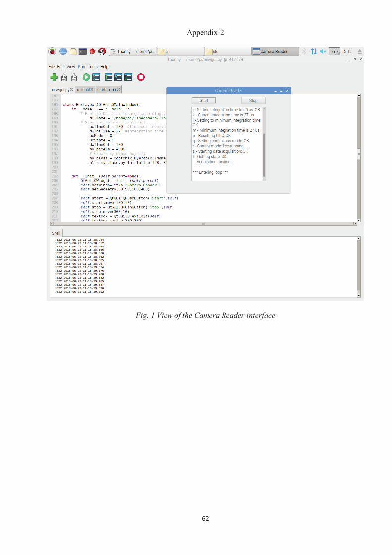
62

Appendix 2

Fig. 1 View of the Camera Reader interface

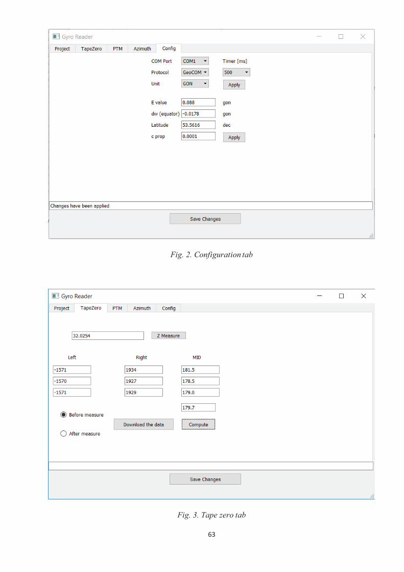
63

Fig. 2. Configuration tab

Fig. 3. Tape zero tab

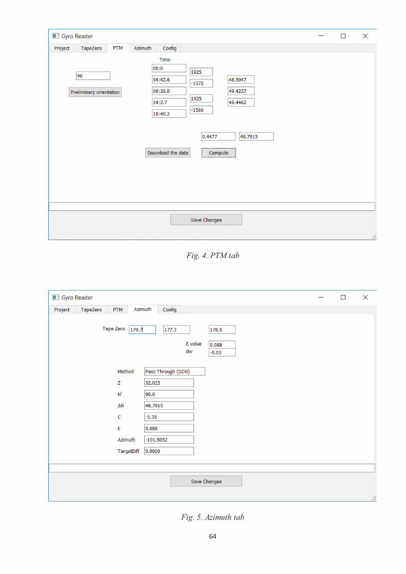
64

Fig. 4. PTM tab

Fig. 5. Azimuth tab

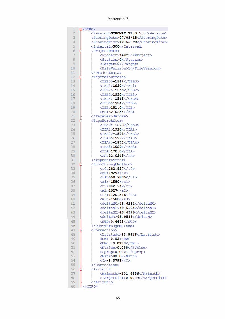
65

Appendix 3