investigations of micromixing - chalmers

Investigations of Micromixing - In Alfa Laval’s ART® Plate Reactors

Master of Science Thesis

ERIK TUNESTÅL Department of Chemical and Biological Engineering Division of Chemical Engineering CHALMERS UNIVERSITY OF TECHNOLOGY Gothenburg, Sweden, 2012

ii


Erik Tunestål © Erik Tunestål, 2012 Department of Chemical and Biological Engineering Chalmers University of Technology SE-412 96 Göteborg Sweden Telephone: +46 (0)31-772 1000 Supervisors: Magnus Lingvall, Alfa Laval and Linus Helming, Alfa Laval Examiner: Ronnie Andersson, Chalmers University of Technology Department of Chemical and Biological Engineering Göteborg, Sweden 2012

iii


ERIK TUNESTÅL Department of Chemical and Biological Engineering Chalmers University of Technology

Abstract This master thesis is investigating the mixing efficiency in Alfa Laval ART® Plate Reactors. The investigation has been performed in the reactor model called PR37, handling flow rates up to 32 l/h. Villermaux/Dushman method also known as Iodide-Iodate method is the method used to measure the segregation index and in the end the mixing time. A range of experiments has been performed and evaluated in order to characterise the behaviour of the reactor in the terms of mixing. The method has been confirmed to work for the ART® Plate Reactor series and with the right auxiliary equipment the whole series of ART® Plate Reactors could be evaluated. The mixing time for the reactor is highly dependent on the flow rate. When first using a flow rate which is half of the recommended and then increasing the flow rate to twice the recommended for PR37 3-12 the mixing time is decreased by more than 75%, when using a 100 µm nozzle. Compared to micromixers the ART® PR37 series performs well. In the comparison of mixing time versus pressure drop the performance is in the same region as for micromixers like IMM Caterpillar, T-mixers and tangential IMTEK. When considering the flow rate also and comparing the mixing time divided by the squared hydraulic diameter and Reynolds number the PR37 series outperforms most the micromixers, it is only the IMM Caterpillar which is in the region of the performance from PR37. Keywords: micromixing, continuous reactor, ART, plate reactor, mixing, iodide-iodate, Villermaux-Dushman

iv

Acknowledgements First of all I would like to thank my main supervisors at Alfa Laval, Magnus Lingvall and Linus Helming, for letting me perform this interesting Master Thesis at Alfa Laval Reactor Technology. I would also like to thank them for their support both with my questions and with the correspondence with other parts of the Alfa Laval. I would also like to thank the rest of the Alfa Laval Reactor Technology Department for making the thesis time an enjoyable period. Especially I would like to thank Kasper Höglund and Barry Johnson for their input and knowledge when discussing different parts of the project, and also an extra thank you to Barry for having me as a flat-mate during my Master Thesis. For the use of the spectrometer equipment I would like to thank Tania Irebo at Azpect Photonics in Södertälje. A special thanks is also sent to Frans Visscher at the Eindhoven University of Technology, he has rapid in response through e-mails and has provided information for the spectrometry set-up. Frans Visscher was also involved in the pre-study performed before this Master Thesis.

v

Table of contents Chalmers University of Technology ............................................................................... iii

Abstract ............................................................................................................................ iii

Acknowledgements ......................................................................................................... iv

Introduction ...................................................................................................................... 1

Mixing Phenomena and its Necessity in Chemical Reactors ........................................ 1

Chemical Reactors......................................................................................................... 1

Details of the ART® Plate Reactor .................................................................................. 3

The Reactor Plates ......................................................................................................... 3

ART® Plate Reactor 37 & LabPlate .......................................................................... 3

ART® Plate Reactor 49 ............................................................................................. 6

Previous micromixing studies .................................................................................... 6

The Goal of the Project ................................................................................................. 6

Experimental Methods ...................................................................................................... 8

Competing Chemical Reactions .................................................................................... 8

Diazo Coupling .......................................................................................................... 9

Villermaux-Dushman Reaction ............................................................................... 10

Villermaux-Dushman Test Reaction System .............................................................. 10

Reaction Kinetics ..................................................................................................... 10

Theoretical Mixing Time ......................................................................................... 12

Segregation Index Xs ............................................................................................... 12

Principle of Iodine Concentration Measurement ..................................................... 13

Calibration Curve for Spectrometer ..................................................................... 13

Micromixing Models ............................................................................................... 14

Interaction-by-exchange-with-mean (IEM) model ............................................... 16

Incorporation model ............................................................................................. 16

The Coalescence and Redispersion Model ........................................................... 16

Engulfment-deformation-diffusion (EDD) model ................................................ 17

Comments on mixing models ............................................................................... 17

Methodology ................................................................................................................... 18

Application of the Villermaux-Dushman test reaction system ................................... 18

Equipment benchmarking / Performance test of equipment ....................................... 19

Proposed experimental design ..................................................................................... 20

Tailoring reaction rates ............................................................................................ 21

Constructing the calibration curve for the spectrometer ............................................. 22

Experimental Setup ........................................................................................................ 24

The Spectrometer ........................................................................................................ 24

Limitations and time restrictions ................................................................................. 25

vi

The use of nozzle ..................................................................................................... 26

Data acquisition ........................................................................................................... 27

Results ............................................................................................................................ 28

The incomparable parameters ..................................................................................... 28

Absorbance .............................................................................................................. 28

Segregation index .................................................................................................... 29

Micromixing model ..................................................................................................... 29

Discussion ....................................................................................................................... 35

Reliability & Reproducibility ...................................................................................... 35

PR37 0.8-2.2 plate ................................................................................................... 35

Nozzle experiments .................................................................................................. 36

Characterisation and comparison ................................................................................ 36

Performance comparison of micromixers ................................................................ 36

A new adaptive procedure for using chemical probes to characterize mixing ........ 39

Comparison with batch reactors .............................................................................. 39

High-Throughput Microporous Tube-in-Tube Microchannel Reactor .................... 40

Pre-study .................................................................................................................. 41

Conclusions .................................................................................................................... 42

Recommendations ....................................................................................................... 42

Future investigations ...................................................................................................... 43

Bibliography ................................................................................................................... 44

Appendix A. Solution preparation ..................................................................................... I

Appendix B. Procedure for calibration ............................................................................. II

Appendix C. Spectrometer instructions .......................................................................... III

Appendix D. Calculations in Excel .................................................................................. V

Appendix E. Concentration ............................................................................................ VI

Appendix F. Absorbance graphs ................................................................................... VII

Appendix G. MatLAB-script for mixing time graph ..................................................... XII

vii

Table of Figures Figure 1. Different parts of a plate for the PR37 reactors. ............................................... 3

Figure 2. An assembled PR37 Reactor with a total of 10 plates. ..................................... 3

Figure 3. Picture of channel design for ART® PR37 and LabPlate plates, this example is the PR37 3-12. .............................................................................................................. 4 Figure 4. Inlet port PR37 0.8-2.2. ..................................................................................... 5 Figure 5. Inlet port PR37 3-12. ......................................................................................... 5 Figure 6. Inlet port PR37 12-46 ........................................................................................ 5 Figure 7. Illustration of the different ports on a plate. ...................................................... 5 Figure 8. Inlet of port 1, N1. ............................................................................................. 5 Figure 9. Inlet of port 2, N2 .............................................................................................. 5 Figure 10. Port inlet design, PR37 3-12 used for the illustration. .................................... 6

Figure 11. Typical concentration versus absorbance graph, image owned by Prof. Tom O'Haver , Professor Emeritus, The University of Maryland at College Park. ................ 14

Figure 12. Adjustment curve for flow meter from the gear pump ................................. 20

Figure 13. Calibration curve ........................................................................................... 23 Figure 14. Schematic over the experimental arrangement ............................................. 24

Figure 15. Typical absorbance spectrum for the iodide-iodate method ......................... 25

Figure 16. An example of vastly differing absorbance result......................................... 28

Figure 17. Measurement of the fluctuations within measurements of segregation index ........................................................................................................................................ 29

Figure 18. Generic image of mixing time calculation .................................................... 30

Figure 19. Mixing time vs. pressure drop, Main in -Main Out ...................................... 31

Figure 20. Mixing time vs. pressure drop, Acid in - Main Out ...................................... 31

Figure 21. Normalised mixing time versus Reynolds number, Port 1. .......................... 31

Figure 22. Mixing time versus energy dissipation, Port 1. ............................................. 32

Figure 23. Sketch of Dean vortices, picture from Palo Alto Research Center. .............. 33

Figure 24. Power regression curves and theoretical trend curves; inverse diffusion coefficients vs. Reynolds number ................................................................................... 33 Figure 25. Inverse diffusion coefficient versus Reynolds for PR37 3-12 plate. ............ 34

Figure 26. Comparative graph using data from (Falk and Commenge, 2010), mixing time versus energy dissipation. ....................................................................................... 37 Figure 27. Comparative graph to data from (Falk and Commenge, 2010), inverse diffusion coefficient versus Reynolds number. .............................................................. 38 Figure 28. Inversed diffusion coefficient versus Reynolds number for different secondary inlet types. ..................................................................................................... 38 Figure 29. Comparison with Assirelli on the base of Reynolds number ........................ 40

Figure 30. PR37 0.8-2.2, 0.5*Nominal, Port 1 .............................................................. VII Figure 31. PR37 0.8-2.2, 1*Nominal, Port 1 ................................................................. VII Figure 32. PR37 3-12, 0.5*Nominal, Port 1 ................................................................. VIII Figure 33. PR37 3-12, 0.5*Nominal, Port 2 ................................................................. VIII Figure 34. PR37 3-12, 1*Nominal, Port 1 .................................................................... VIII Figure 35. PR37 3-12, 1*Nominal, Port 2 ...................................................................... IX

Figure 36. PR37 3-12, 2*Nominal, Port 1. ..................................................................... IX

Figure 37. PR37 3-12, 2*Nominal, Port 2 ...................................................................... IX

Figure 38. PR37 12-46, 0.5*Nominal, Port 1. .................................................................. X

Figure 39. PR37 12-46, 1*Nominal, Port 1. ..................................................................... X

Figure 40. PR37 3-12, 0.5*Nominal, Port 1 and 2, Nozzle .............................................. X

Figure 41. PR37 3-12, 1*Nominal, Port 1 and 2, Nozzle ............................................... XI

Figure 42. PR37 3-12, 2*Nominal, Port 1 and 2, Nozzle ............................................... XI

viii

Table of Tables Table 1. Experimental methods for characterizing micromixing, (Aubin et al., 2010).... 8

Table 2. Estimated mixing times calculated from pressure drop data from 2008. ......... 18

Table 3. Flow rates needed for the buffer solution to achieve 0.2 m/s flow .................. 19

Table 4. Initial experimental design ............................................................................... 20 Table 5. Linear velocities using the general flow rates .................................................. 21 Table 6. Used volume and length for reactor characterization ....................................... 21

Table 7. Reaction time calculations from initial concentrations .................................... 22

Table 8. Mixing table and absorbance results for calibration curve ............................... 23

Table 9. The performed experiments during the project ................................................ 26

Table 10. Change in inlet velocity when using nozzle. .................................................. 26

Table 11. Absorbance data from the experiments .......................................................... 28

Table 12. Mixing time for the 16 different flow conditions ........................................... 30

Table 13. The micromixing results from the Assirelli study .......................................... 40

Table of Equations (1) ................................................................................................................................... 11

(2) ................................................................................................................................... 11

(3) ................................................................................................................................... 11

(4) ................................................................................................................................... 11

(5) ................................................................................................................................... 11

(6) ................................................................................................................................... 11

(7) ................................................................................................................................... 12

(8) ................................................................................................................................... 12

(9) ................................................................................................................................... 12

(10) ................................................................................................................................. 12

(11) ................................................................................................................................. 12

(12) ................................................................................................................................. 12

(13) ................................................................................................................................. 12

(14) ................................................................................................................................. 13

(15) ................................................................................................................................. 13

(16) ................................................................................................................................. 13

(17) ................................................................................................................................. 13

(18) ................................................................................................................................. 13

(19) ................................................................................................................................. 13

(20) ................................................................................................................................. 16

(21) ................................................................................................................................. 16

(22) ................................................................................................................................. 16

(23) ................................................................................................................................. 16

(24) ................................................................................................................................. 16

(25) ................................................................................................................................. 17

(26) ................................................................................................................................. 17

(27) ................................................................................................................................. 23

1

Introduction The goal of this project is to both find a method to characterize the Micromixing in Alfa Laval’s ART® Plate Reactors and to perform the characterization for some of the configurations within the ART® Plate Reactor series. The present section consists of two parts, an introduction to the concept of mixing and its importance for chemical reactors and the second part is introducing chemical reactors and the ART® Plate Reactor series.

Mixing Phenomena and its Necessity in Chemical Reactors In chemical reaction and thereby chemical reactors mixing is a fundamental unit operation, especially in industrial applications such as chemistry, pharmaceutical and polymers where a high yield is important (Habchi et al., 2011). Without mixing the different substances won’t come in contact with each other and no reaction occurs. Baldyga (Bałdyga and Bourne, 1999) and others (Fournier et al., 1996b); (Johnson and Prud'homme, 2003) have introduced the concept of dividing the mixing into three stages with different length scales of mixing. These three scales are macro-, meso- and micromixing, in turbulent mixing the turbulent energy is dissipated down from macro-scale mixing down to micromixing and ultimately down to laminar lamellae where molecular diffusion is the driving force. The macro-mixing is of the scale of the entire reactor, it is the simplest way to characterize a reactor. Despite the development of CFD codes residence time distribution experiments remains the standard way of characterizing complex flows (Villermaux, 1996). Meso-mixing is generally the scale of turbulent diffusion. The scale is fine respective to the system but coarse respective to micromixing e.g. the turbulent exchange between the feed and bulk near the inlet of a reactor with a fast reaction (Bałdyga and Pohorecki, 1995). Micromixing is the mixing which takes place on molecular scale, below the so called Batchelor scale. In this region it is laminar stretching which leads to interlacing of the laminar layers thereby increasing the mixing and reaction i.e. the mass transfer is dominated by molecular diffusion. (Habchi et al., 2011) The process can also be described as the viscous-convective deformation of fluid elements which, when the deformation is large enough, is followed by molecular diffusion. Micromixing is especially important for chemical processes with fast reaction kinetics (Guichardon et al., 2001). Chemical reactions occur on molecular level (Bałdyga and Pohorecki, 1995) and micromixing significantly affects the conversion and selectivity for fast and instantaneous reactions, both in laminar and turbulent flows. A higher mixing on the molecular scale will increase the interfacial area between the two phases massively i.e. more contacts being made (Aubin et al., 2010). The micromixing will, for fast reactions, affect various process parameters such as yield, reaction time, mass- and heat transfer. The mixing is most important if the system contains multiple reactions, if there are no side reactions the mixing only affects the reaction time. If side reactions are present poor mixing increases the probability of the side reactions occurring and lowers selectivity.

Chemical Reactors Traditionally the reactions for production of specialty chemicals, e.g. for the pharmaceutical industry, have taken place in stirred batch reactors. This has been the

2

case for both single and multiphase reactions. The tank reactors are familiar and numerous equations for prediction of power consumption and mass transfer exist. However they also have some significant drawbacks including scale-up, mixing and hold-up time if continuous. The scale-up from laboratory scale to production scale is always uncertain (Bouaifi et al., 2004). Especially the heat transfer will change in a scale-up and significantly change the yield of the reactions (Hendershot and Sarafinas, 2005). The ART® Plate Reactor proposes a solution to these problems in being an easily scalable continuous reactor. The ART® Plate Reactors are a reactor series with a large range of flows from 120 mL/h up to 1000 L/h and residence times from 4 seconds up to 25 minutes. This combined with very high heat transfer ability is making the ART® Plate Reactor series a feasible alternative for a wide range of applications, such as production of organic silica monomers. (AlfaLaval, 2005b, AlfaLaval, 2005c, AlfaLaval, 2005a)

3

Details of the ART® Plate Reactor At present the Alfa Laval ART Plate Reactor series consists of three commercially available reactor types. The ART Plate Reactor (PR) 37 which handles up to 10 plates and flows up to about 32 l/h. The ART LabPlate which is a downsized ART PR37 the difference is that the ART LabPlate only handles two plates and thereby smaller flows of up to 2.4 l/h with the benefit of being more cost efficient for these flows. The last type is the ART PR49 which is a larger scale up from the ART PR37. The ART PR49 has another type of mechanical construction, another assembly of plates and handles much higher flow rates, up to 1000 l/h. The ART PR49 is designed to be large enough to be used in commercial production, whereas the ART PR37 and LabPlate are primarily aimed for research & development and production in small scale.

The Reactor Plates The ART LabPlate is using the PR37 0.8-2.2 and PR37 3-12 plates with the same design as the ones used for PR37. The larger ART® PR49 has another frame design and significantly larger plates.

ART® Plate Reactor 37 & LabPlate The plates in the reactors consist of a process side and a utility side, illustrated in Figure 1. The plate consists of five different components. Number 1 is the process channel plate, this is the plate to which inlets and outlets for the process and utility are fitted, and the bottom side has a 2 mm deep channel to form the utility side, the channel is as wide as the entire plate. The utility side is also made turbulent using a turbulator plate, number 2. The utility pressure plate, number 3, seals the utility side and the process gasket, 4, and pressure plate, 5, does the same for the process side. When all the desired number of plates is assembled the stack is pressed together using tension rods forming a reactor seen in Figure 2.

Figure 1. Different parts of a plate for the PR37 reactors.

Figure 2. An assembled PR37 Reactor with a total of 10 plates.

The design characteristic of the ART Plate Reactors is the serpentine path which the process flow follows in the process channel plate. This path is also in an alternating sequence becoming wider and narrower. This induces stretching and contraction of the flow and also the serpentine path is creating vortices in the channel. These “chaotic” features of the design are creating a very good mixing, in laminar flow (Ehrfeld et al., 1999). Despite this chaotic behaviour of the channel the reactor has an excellent plug flow (AlfaLaval, 2005b).

4

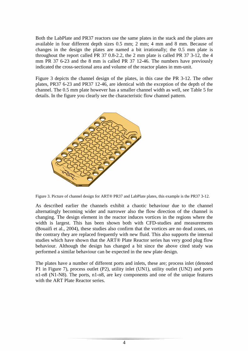
Both the LabPlate and PR37 reactors use the same plates in the stack and the plates are available in four different depth sizes 0.5 mm; 2 mm; 4 mm and 8 mm. Because of changes in the design the plates are named a bit irrationally; the 0.5 mm plate is throughout the report called PR 37 0.8-2.2, the 2 mm plate is called PR 37 3-12, the 4 mm PR 37 6-23 and the 8 mm is called PR 37 12-46. The numbers have previously indicated the cross-sectional area and volume of the reactor plates in mm-unit. Figure 3 depicts the channel design of the plates, in this case the PR 3-12. The other plates, PR37 6-23 and PR37 12-46, are identical with the exception of the depth of the channel. The 0.5 mm plate however has a smaller channel width as well, see Table 5 for details. In the figure you clearly see the characteristic flow channel pattern.

Figure 3. Picture of channel design for ART® PR37 and LabPlate plates, this example is the PR37 3-12.

As described earlier the channels exhibit a chaotic behaviour due to the channel alternatingly becoming wider and narrower also the flow direction of the channel is changing. The design element in the reactor induces vortices in the regions where the width is largest. This has been shown both with CFD-studies and measurements (Bouaifi et al., 2004), these studies also confirm that the vortices are no dead zones, on the contrary they are replaced frequently with new fluid. This also supports the internal studies which have shown that the ART® Plate Reactor series has very good plug flow behaviour. Although the design has changed a bit since the above cited study was performed a similar behaviour can be expected in the new plate design. The plates have a number of different ports and inlets, these are; process inlet (denoted P1 in Figure 7), process outlet (P2), utility inlet (UN1), utility outlet (UN2) and ports n1-n8 (N1-N8). The ports, n1-n8, are key components and one of the unique features with the ART Plate Reactor series.

5

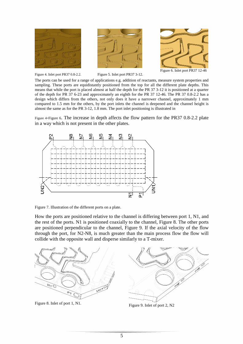
Figure 4. Inlet port PR37 0.8-2.2.

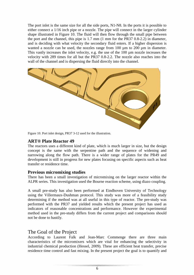
Figure 5. Inlet port PR37 3-12.

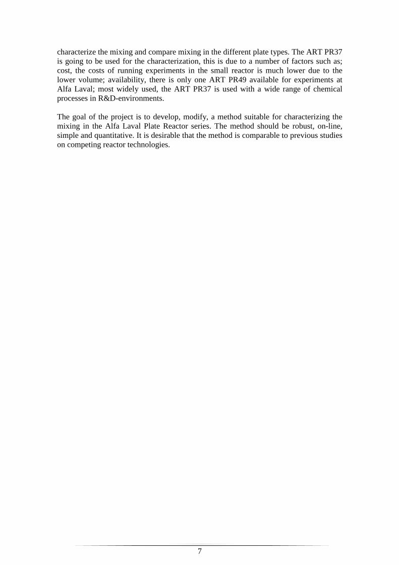
Figure 6. Inlet port PR37 12-46

The ports can be used for a range of applications e.g. addition of reactants, measure system properties and sampling. These ports are equidistantly positioned from the top for all the different plate depths. This means that while the port is placed almost at half the depth for the PR 37 3-12 it is positioned at a quarter of the depth for PR 37 6-23 and approximately an eighth for the PR 37 12-46. The PR 37 0.8-2.2 has a design which differs from the others, not only does it have a narrower channel, approximately 1 mm compared to 1.5 mm for the others, by the port inlets the channel is deepened and the channel height is almost the same as for the PR 3-12, 1.8 mm. The port inlet positioning is illustrated in

Figure 4-Figure 6. The increase in depth affects the flow pattern for the PR37 0.8-2.2 plate in a way which is not present in the other plates.

Figure 7. Illustration of the different ports on a plate.

How the ports are positioned relative to the channel is differing between port 1, N1, and the rest of the ports. N1 is positioned coaxially to the channel, Figure 8. The other ports are positioned perpendicular to the channel, Figure 9. If the axial velocity of the flow through the port, for N2-N8, is much greater than the main process flow the flow will collide with the opposite wall and disperse similarly to a T-mixer.

Figure 8. Inlet of port 1, N1.

Figure 9. Inlet of port 2, N2

6

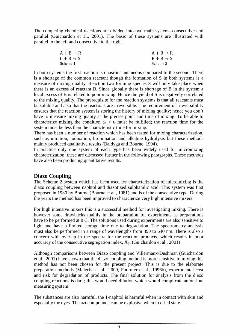
The port inlet is the same size for all the side ports, N1-N8. In the ports it is possible to either connect a 1/16 inch pipe or a nozzle. The pipe will connect in the larger cylinder shape illustrated in Figure 10. The fluid will then flow through the small pipe between the port and the channel, this pipe is 1.7 mm (1 mm for the PR37 0.8-2.2) in diameter, and is deciding with what velocity the secondary fluid enters. If a higher dispersion is wanted a nozzle can be used, the nozzles range from 100 µm to 200 µm in diameter. This vastly increases the inlet velocity, e.g. the use of the 100 µm nozzle increases the velocity with 289 times for all but the PR37 0.8-2.2. The nozzle also reaches into the wall of the channel and is dispersing the fluid directly into the channel.

Figure 10. Port inlet design, PR37 3-12 used for the illustration.

ART® Plate Reactor 49 The reactors uses a different kind of plate, which is much larger in size, but the design concept is the same with the serpentine path and the sequence of widening and narrowing along the flow path. There is a wider range of plates for the PR49 and development is still in progress for new plates focusing on specific aspects such as heat transfer or residence time.

Previous micromixing studies There has been a small investigation of micromixing on the larger reactor within the ALPR series. This investigation used the Bourne reaction scheme, using diazo coupling. A small pre-study has also been performed at Eindhoven University of Technology using the Villermaux-Dushman protocol. This study was more of a feasibility study determining if the method was at all useful in this type of reactor. The pre-study was performed with the PR37 and yielded results which the present project has used as indicators of reasonable concentrations and performance. However the experimental method used in the pre-study differs from the current project and comparisons should not be done to hastily.

The Goal of the Project According to Laurent Falk and Jean-Marc Commenge there are three main characteristics of the micromixers which are vital for enhancing the selectivity in industrial chemical production (Hessel, 2009). These are efficient heat transfer, precise residence time control and fast mixing. In the present project the goal is to quantify and

7

characterize the mixing and compare mixing in the different plate types. The ART PR37 is going to be used for the characterization, this is due to a number of factors such as; cost, the costs of running experiments in the small reactor is much lower due to the lower volume; availability, there is only one ART PR49 available for experiments at Alfa Laval; most widely used, the ART PR37 is used with a wide range of chemical processes in R&D-environments. The goal of the project is to develop, modify, a method suitable for characterizing the mixing in the Alfa Laval Plate Reactor series. The method should be robust, on-line, simple and quantitative. It is desirable that the method is comparable to previous studies on competing reactor technologies.

8

Experimental Methods Over the past 20 years since micro mixers became commercially available many papers and studies have been undertaken to quantify the potential gain of these micro mixers. Unfortunately though these gains have mostly been determined for specific reactions, only a fraction of the studies have been characterizing the micro mixing unit itself. (Commenge and Falk, 2011) The present project however is aiming for exactly that, a characterization of micromixing in the Alfa Laval ART® plate reactor series. The design of the ART® Plate Reactor imposes some restrictions on the choice of characterization method. Because the plates of the reactor are of metal no optical transparency to the reactor is available. In the survey of feasible methods emphasis has been put to the method being robust, simple and on-line. The experimental cost has also been a factor in the choice of method. Different methods have been examined in a literature survey and many methods have been identified unfortunately the majority of these methods require optical access, if not to the entire reactor at least to some specific places. In the present project no optical access to the reactor is available. A list of numerous methods and their corresponding prerequisites on the reactor are listed in Table 1 they have been more thoroughly investigated by Aubin (Aubin et al., 2010). The results from Aubin have been extended to include both consecutive and parallel chemical reactions. The method chosen for the present project is competitive chemical reactions, mainly because optical transparency is unavailable.

Table 1. Experimental methods for characterizing micromixing, (Aubin et al., 2010)

Method Resulting information Micro device requirements

Dilution of coloured dyes

Qualitative information on mixing quality Indirect approximation of mixing time

Transparent device or device with transparent viewing window

Dilution of fluorescent species

Qualitative information on mixing quality Indirect approximation of mixing time 3D concentration maps possible


Acid-base or pH indicator reactions



Reactions yielding coloured species



Competitive chemical reactions

Quantitative information on the yield of the secondary reaction. Mixing time calculated indirectly from concentration measurements.

No particular for off-line method. For on-line measurements using UV-Vis spectroscopy, measurement cell must be transparent.

Monitoring species concentrations

1-dimensional profiles or 2-dimensional maps of species concentration. Can identify the characteristic scale of fluid lamellae which can be related to mixing.

Either optically transparent for visible light or infrared.

Competing Chemical Reactions The method competing chemical reactions is one of three types under the classification reaction-based characterization. The other two are acid-base reactions and reactions yielding coloured species both of these requires optical access to the reactors (Aubin et al., 2010).

9

The competing chemical reactions are divided into two main systems consecutive and parallel (Guichardon et al., 2001). The basic of these systems are illustrated with parallel to the left and consecutive to the right. A + B → R C + B → S

Scheme 1

A + B → R R + B → S Scheme 2

In both systems the first reaction is quasi-instantaneous compared to the second. There is a shortage of the common reactant though the formation of S in both systems is a measure of mixing quality. Reaction two forming species S will only take place when there is an excess of reactant B. Since globally there is shortage of B in the system a local excess of B is related to poor mixing. Hence the yield of S is negatively correlated to the mixing quality. The prerequisite for the reaction systems is that all reactants must be soluble and also that the reactions are irreversible. The requirement of irreversibility ensures that the reaction system is storing the history of mixing quality; hence you don’t have to measure mixing quality at the precise point and time of mixing. To be able to characterize mixing the condition tm > tr must be fulfilled; the reaction time for the system must be less than the characteristic time for mixing. There has been a number of reaction which has been tested for mixing characterization, such as nitration, iodination, bromination and alkaline hydrolysis but these methods mainly produced qualitative results (Baldyga and Bourne, 1994). In practice only one system of each type has been widely used for micromixing characterization, these are discussed further in the following paragraphs. These methods have also been producing quantitative results.

Diazo Coupling The Scheme 2 system which has been used for characterization of micromixing is the diazo coupling between naphtol and diazotized sulphanilic acid. This system was first proposed in 1980 by Bourne (Bourne et al., 1981) and is of the consecutive type. During the years the method has been improved to characterize very high intensive mixers. For high intensive mixers this is a successful method for investigating mixing. There is however some drawbacks mainly in the preparation for experiments as preparations have to be performed at 0 C. The solutions used during experiments are also sensitive to light and have a limited storage time due to degradation. The spectrometry analysis must also be performed in a range of wavelengths from 390 to 640 nm. There is also a concern with overlap in the spectra for the reaction products, which results in poor accuracy of the consecutive segregation index, XS. (Guichardon et al., 2001) Although comparisons between Diazo coupling and Villermaux-Dushman (Guichardon et al., 2001) have shown that the diazo coupling method is more sensitive to mixing this method has not been chosen for the present project. This is due to the elaborate preparation methods (Malecha et al., 2009, Fournier et al., 1996b), experimental cost and risk for degradation of products. The final solution for analysis from the diazo coupling reactions is dark; this would need dilution which would complicate an on-line measuring system. The substances are also harmful, the 1-naphtol is harmful when in contact with skin and especially the eyes. The azocompounds can be explosive when in dried state.

10

Villermaux-Dushman Reaction The Villermaux-Dushman also known as iodide-iodate test reaction system is a system of the type described in Scheme 1. The first reaction is quasi-instantaneous and the reaction time of the second can be adjusted by the concentration of species C. This feature that you can adjust the reaction speed of the second reaction means that you can tailor the reaction system to make very local measurements or more global (Habchi et al., 2011). The iodide-iodate method is an easy method using common chemicals and normal operating conditions. It produces consistent results and comparing different reactors or operating conditions is possible using the same experimental setup. Quantitative comparisons, e.g. comparing experiments performed with different concentrations or volume ratios, cannot be made with this method (Malecha et al., 2009, Bourne, 2008) because the kinetics of the Dushman reaction are still not perfectly known under the experimental conditions which is required. But methods for overcoming this problem using a characteristic mixing time have been investigated and comparisons are possible within accuracy limits, according to (Falk and Commenge, 2010) an accuracy of more than 30% cannot be expected. Since the mixing time is relatively fast a good estimation can be achieved despite the accuracy limitation, it is sufficient with knowing that the mixing time is in the region of 0.1±0,03s. The Villermaux-Dushman method is suitable for making qualitative comparisons when the experimental conditions are constant. This makes it suitable for the present project since the main goal is to derive a method for comparing different plate designs and flow conditions. This means that the same ratio and concentrations can be used throughout the experimental series. Comparisons can also be made in-house with other types of reactors e.g. tubular reactors. The Villermaux-Dushman method has been chosen as test reaction for the present project.

Villermaux-Dushman Test Reaction System The reactions system is commonly used but there is no general method for setting up experiments. There are however a number of reports trying to formulate a stringent experimental setup for this method (Commenge and Falk, 2011, Guichardon et al., 2001, Fournier et al., 1996b). But there are always some parameters which have been specified specifically for the proposed methodology e.g. flow ratio and concentrations. One of those examples is the detailed approach proposed by Commenge and Falk which unfortunately is considered for reactors using the same flow rate in both the buffer- and acid stream, e.g. in T- and V-mixers. In the ART Plate Reactors it is not suitable to have the same flow rate in both process streams since this would yield a much higher pressure drop in the ports, since they have a smaller cross-sectional area. This pressure drop in itself would affect the mixing characteristics significantly. These variations and the debated kinetics, which will be discussed further later, make direct quantitative comparisons impossible.

Reaction Kinetics The Villermaux-Dushman test reaction system is based upon three different reactions. The first two reactions are part of a competitive reaction system. This reaction system is an acid-base neutralization ( i ) and an oxidation ( ii ). The oxidation reaction ( ii ) is called the Dushman reaction. The reactions are: �� + � ⇌ �� ( i )

11

5�� + �� + 6� ⇌ 3� + 3� ( ii ) The neutralization reaction ( i ) is quasi-instantaneous with respect to the Dushman reaction ( ii ). This vast difference in reaction time is the quality which makes this reaction system suitable for characterizing mixing. Using different concentrations of the chemicals the reaction rate of the second reaction ( ii ) can be tailored for the specific reactor system. The reaction kinetics for the Dushman reaction has been a major debate for the reaction system. Guichardon and Falk have performed a major kinetic study of the reaction (Guichardon et al., 2000) and the reaction expression they suggests is also the one used in the present project. The suggested reaction kinetics is: �� = �� (1)

The reaction expression in itself might not look too complicated, a five order reaction. The kinetics studies however show that the rate expression has a so called salt effect. The reaction constant is dependent upon the ionic strength, �. The expressions brought forward by Guichardon and Falk are: � < 0,166 : "#$%&'�( = 9,28105 − 3,664.� (2)

� > 0,166 : "#$%&'�(= 8,383 − 1,5112.� + 0,23689� (3)

� = 12 ∗ 1 2343

3 (4)

The ionic strength of the solution is determined by the concentration of each ion, c, and the charge of the ion, z, to the power of two. From the reaction kinetics of reaction ( ii ) and initial concentrations of the buffer solution and acid a reaction time for the ( ii ) reaction can be calculated, by dividing the stoichiometric concentration with the reaction rate.

56�� = 78 935 ��&; 3�� &; 12 ��&;'��(<=& (5)

The formed iodine, �, from the ( ii ) reaction further reacts into � � following the quasi-instantaneous equilibrium: � + �� ⇌ � � ( iii ) The equilibrium constant for this reaction is a function of temperature and defined by (Palmer et al., 1984);

"#$%& >? = @@@A + 7,355 − 2,575 "#$%& C, (6)

where KB is the equilibrium constant for reaction ( iii ) and T is the temperature in Kelvin. The kinetics of this reaction,( iii ), have been studied by (Ruasse et al., 1986) and the reaction rates of the reaction in water solution at 25 °C has been determined to:

12

�� = � �� − � �� (7)

,where � � = 5,6 × 10E " ∙ G#"�%H�% and � � = 7,5 × 10I H�%

Theoretical Mixing Time For the Villermaux-Dushman characterization the best sensitivity is achieved when 56�� ≈ 5Kwhere 5K is a characteristic time for mixing. In accordance with the protocol designed by Commenge and Falk (Commenge and Falk, 2011) an estimated mixing time can be calculated using the pressure drop. In mixing there is always a trade-off between pressure drop and mixing time (Kashid et al., 2011), faster mixing inevitably means higher pressure drop. Pressure drop measurements have been performed previously for the ART Plate Reactors. The measurements have been performed using water and the flow rate is ranging from zero to twice the nominal flow. The equations for estimating mixing time are: L = M ∗ NO

P ∗ Q (8)

5K = 0.15 ∗ L�&.S@, (9) where Q is the flow rate [m3/s], ∆P is pressure drop [Pa], ρ is density [kg/m3], V is the volume of reactor [m3] and ε is energy dissipation [W/kg]. The theoretical mixing time indicates how fast mixing to expect from the reactor. However this is not the only parameter deciding how fast the ( ii ) should be. If the reaction time is too short the experiments will only measure the mixing at the inlet. In this project it is the design and mixing efficiency of the channel which is the interesting parameter and how effective the nozzle at the inlet is.

Segregation Index Xs The segregation index is an index used to quantify the micromixing quality explicitly. The segregation index range from 0 to 1, where 1 means that the flow is totally segregated and 0 that perfect mixing has occurred. The values in between indicates partial mixing. The formula for segregation index is: TU = V

VAU (10)

V = 2W8XY + 8XZ[\8]_̂ = 2 `ab<'�� + �� (

`cd�e��& (11)

VAU = 6�� &6�� & + �� & (12)

TU = 2 `ab<'�� + �� (`cd�e��& × f1 + �� &6�� & g

(13)

The concentration of iodine, �, and triiodide ions, � �, are the unknowns in the equation for segregation index. The mass balance of iodine atoms combined with the equilibrium constant for reaction ( iii ) yields an equation system which decreases the degrees of freedom to one;

13

àb<�� = `hbiij6̂ ��&− àb< k5

3 '�� + �� ( + �� l (14)

>? = �� (15)

53 àb<�� + k8

3 àb<�� − `hbiij6&��&l ��+ �� àb<>? = 0

(16)

Principle of Iodine Concentration Measurement The concentration of iodine can be measured using spectrometry and the application of Lambert-Beer law. Lambert-Beer law states that the absorption, A, is proportional to the concentration of � �. The proportionality constant is a product of L, known as the molar extinction coefficient, and the path length of the spectrometer, l.

�� = mL" (17)

The absorption of � � is measured at a wavelength of 353 nm where the absorption is not affected by the other compounds in the solution. The second-order algebraic equation, (16), can be solved for the measured concentration of � �. From the solution XS can be calculated using equation (13). The segregation index is dependent upon the concentrations and flows used during the experiments; hence it is not possible to compare mixing quality using XS as a performance indicator.

Calibration Curve for Spectrometer When using an in-line flow cell there are a number of settings which are affecting the signal received in the graphs. The fact that it is possible to manipulate the absorption value means that it is not possible to use a generic value for the molar extinction coefficient. Measuring concentration from the spectrometer absorbance measurements requires a calibration curve. The calibration curve is determined using a number of solutions with differing, known, concentration of the current species, here � �. To prepare solutions of � � with determined concentration mixtures of � and >� in aqueous solution is required. The mixing of these two aqueous solutions will initiate the equilibrium reaction ( iii ). Rewriting the equation for the equilibrium constant (15) in terms of conversion of � (18) generates an equation with only the conversion unknown (19).

�� = TXYQXY��&Q<a< (18)

>? = �XZ[��XY��X[� =

noYpoY�oY�^pqrq's[noY(poY�oY�^

pqrqpto�o[�^[noYpoY�oY�^

pqrq=

uvqrq'%�u('vto�X[�^�voY�XY�û( ,

(19)

where TXYis the conversion of � and Qu is the volume of species X added to the total solution, hence Q<a< = QXY + QwX + Q]Yx.

14

The equilibrium constant can be calculated from (15) and the other variables in (19), except for the conversion are measured during the calibration procedure. From the calculated conversion the concentration of � � can be determined. Measuring the absorbance from a number of solutions containing various concentrations of � � a graph of absorbance versus concentration can be obtained. The graph should resemble Figure 11, where the Lambert-Beer law (17) is valid for the linear relation present up to a certain concentration.

Figure 11. Typical concentration versus absorbance graph, image owned by Prof. Tom O'Haver , Professor Emeritus, The University of Maryland at College Park.

During the experiments the measured absorbance must be within the Lambert-Beer range, otherwise it will not be possible to determine the concentration of� � accurately.

Micromixing Models In order to achieve a comparable parameter the segregation index must be converted into a characteristic mixing time. In order to determine a mixing time perfect knowledge including a full description of velocity and concentration should be needed. In reactive flows that would necessitate a resolution down to Batchelor scale, ~ several microns, for the description of stretching, diffusion and transport coupled with the reaction occurring (Falk and Commenge, 2010). For all but the very simplest geometries this is impossible to achieve. As an alternative solution many researches have proposed various phenomenological models to describe the mixing phenomena. They are based on different assumptions about the limiting processes in the mixing. Mixing can be described by a sequence of mixing mechanisms found in List 1 and List 2. This sequence differs for laminar and turbulent mixing and because of the chaotic nature of the ART Plate Reactor this reactor type could show behaviours from both laminar and turbulent mechanisms. The flow conditions for the current project is in the laminar or at most approaching the transitional region with Reynolds numbers up to 1700, using hydraulic diameter for rectangular conduits. List 1. The mechanism sequence for turbulent mixing:

1. Distributive mixing; large eddies move around and convect material. At macroscopic scale concentration is uniform. No mixing occurs on scale smaller than the size of eddies though.

2. Dispersive mixing; through turbulent shear the above eddies decrease in size and mixing occurs on a finer scale. At molecular scale still no mixing occurs.

15

3. Diffusive mixing; mixing due to the random motion of molecules. Becomes important when the structure is very fine since diffusion only occurs over short distances. The mixture becomes homogenous. The mass transfer and momentum transfer have

similar time scales (Kockmann, 2008). 5? ≈ 5w = 9yz;sY this relation

will be used to evaluate how well the results fit turbulent theory. The correlation between the Batchelor time scale and Kolmogorov time scale is equal when the Schmidt number is around 1000, e.g. for water.

List 2. The mechanisms for laminar mixing:

• Laminar shear; deformation of fluid elements due to relative motion between the fluids. The deformation will increase interfacial area and reduce the thickness of fluid element.

• Elongational or extensional flow; changes is the flow geometry accelerates and decelerates the flow, the effects are similar to the effects of laminar shear, but are induced by the geometry.

• Distributive mixing; reduction of the striation thickness due to stream-splitting and recombination effects in the geometry of the mixer.

• Molecular diffusion; as in turbulent mixing becomes important once striation thickness is short enough.

• Stresses in laminar flow; mixing taking place due to stresses exceeding the bonding force of agglomerates hence dissolving the agglomerates. This mechanism is present in solid-liquid systems.

(Bourne, 1997, Edwards, 1997) For turbulent mixing this sequence can occur successively or simultaneously (Baldyga and Bourne, 1994). In laminar mixing there is not a clear sequence of mixing as in the turbulent case, instead the different mechanisms are present in different types of laminar mixing equipment. There are a number of different proposed models for micromixing. The micromixing models can be divided into three categories; phenomenological, physical and detailed analytical. The detailed analytical type is the method of using detailed descriptions of the fluid dynamics to simulate the mixing using computational fluid dynamics (CFD). Since the ART Plate Reactor is a complex geometry a CFD solution for this project would require a lot of computational power and also license to computer software on this basis the method is excluded for the current project. Phenomenological models involve similar phenomena as the normal RTD models but on a finer scale, the phenomena are e.g. segregated zones and exchange of fluxes. From phenomenological models parameters characteristic for the system are not known a priori (Villermaux and Falk, 1994). The third category of models is physical models. These are based on physical processes in mixing. The models are simplifications of the real mixing process and the goal is that the parameters they are based upon can be independently defined from fluid dynamics or experimental measurements. The physical models validity is corresponding with the

16

assumptions made, the model allows a priori predictions as long as the parameters in the model can be estimated accurately.

Interaction-by-exchange-with-mean (IEM) model One of the phenomenological models is the interaction by exchange with the mean (IEM) model. The model which was proposed, independently, by (Villermaux and Devillon, 1972, Costa and Trevissoi, 1972, Harada et al., 1962) is based upon the assumption of points with uniform concentration and negligible mass interacts with the entire volume consisting of two types of points (the considered and the rest). The entire volume has the mean concentration2�̅. The interaction is linear following the expression: �K(2�̅ − 2�), (20)

where km is an exchange factor which is not easily defined but can be related to power consumed in agitating the fluid. An unsteady mass balance for the concentration at point ci is: ed|

e} = �K(2�̅ − 2�) + ~� , (21)

where � is the age of the point.

Incorporation model Fournier and his colleagues proposed a simple dilution-reaction model for estimating the mixing time (Fournier et al., 1996a). It has been developed and used widely because of its simplicity. The model is suitable for batch systems or plug-flow systems (Fournier et al., 1996a). The original model proposed by Fournier is: e��

e< = W�3%& − �3\ %�e�e< + ~3 , (22)

where �3 is the concentration of reactant j, �3%& the concentration of the surrounding liquid, ~3 the reaction term and g is a function for the mass exchange rate between the fluid parcels and surrounding liquid. The idea behind the model is that the second fluid, which has a much lower volume than the other, is divided into small aggregates. The agglomerates are invaded by the first fluid and the volume of the aggregate (containing both liquid 1 and 2) is increasing. The incorporation time, the time for when the liquid 2 has fully reacted with liquid 1, is equal to the micromixing time in this model. The mass exchange rate function, g, is dependent upon the incorporation mechanism. The incorporation flow could either be constant which means g(t) is a linear function (23) or the flow could be proportional to the aggregate volume resulting in an exponential relation (24).

$(5) = 1 + 55K

(23) $(5)= �� k 55Kl

(24)

The Coalescence and Redispersion Model Initially derived, by Rietema (1958), Harada (1962) and Curl (1963) cited in (Baldyga and Bourne, 1994), to describe the nature of droplets in a two-liquid phase system. It has since been adapted to simulate single-phase flows as well. The concept is that the

17

volume of the system is divided into a number of fluid elements of the same volume and sufficiently many to achieve separation of scales. The fluid elements can mix with each other by coalescence, perfect mixing on molecular scale and immediate redispersion. Using methods like e.g. the Monte Carlo process or probability density functions (pdf) the model can be simulated. The model can be used to determine both micro- and macromixing (Baldyga and Bourne, 1994). The IEM model is closely connected to this model and Harada even proposed the equation (21) to describe the coalescence and redispersion of reactive droplets (Harada et al., 1962) cited in (Baldyga and Bourne, 1994).

Engulfment-deformation-diffusion (EDD) model The EDD model utilizes all three mechanisms involved in micromixing. A reagent volume is incorporated, stretched and folded until the volume elements are of Batchelor scale where molecular diffusion is having an effect. The EDD model becomes quite complex and computationally advanced because it includes all three mechanisms. The method requires solution of equations like

�� + �(�, �)

�� = ��

�� + ��(�, �) (25)

These are coupled, non-linear, parabolic partial differential equation the equations must also be solved a number of times equal to the number of vortex generations needed to achieve complete micromixing. Baldyga and Bourne (Baldyga and Bourne, 1989) have

in the report showed that under certain circumstances, �2 ≪ 4000 �8� � 9= d�^d�^; ≫ 1,

the deformation and diffusion can be neglected. This simplifies the model significantly to a set of ordinary differential equations of the type:

ed|e} = �'⟨2�⟩ − 2�( + ~� , (26)

where E is an engulfment rate. The simplified model is consequentially called the engulfment model or E-model. Note the resemblance to the incorporation model, equation (22) with the exponential relation (24).

Comments on mixing models Though the models are based on different assumptions and principles many of them share the characteristic looks of the equations to be solved. But even though they may look similar equations (21) and (26) produce different results (Baldyga and Bourne, 1990) in this case because of how the mixed zone is handled. In the E-model it is growing with time, but in the IEM model the volume is always infinitely small. In the current project the reactor has a very good plug-flow which is why the incorporation model is chosen. The incorporation flow is said to be proportional to the aggregate volume, using (24). That the incorporation flow would be proportional seems to be the most logic assumption, that a larger volume faster incorporates more volume.

18

Methodology Following the theoretical background of the project which has been presented up until now the following sections will be describing how the experiments during this project have been performed. This includes the motivation behind experimental setup, equipment usage and limitations.

Application of the Villermaux-Dushman test reaction system As described in the theoretical section (8), (9), a theoretical mixing time can be calculated if the pressure drop is known for the reactor. The results from the estimation of mixing time for the different plates can be found in Table 2. As can be expected the mixing time varies with the flow rate. When the flow rate changes from half the nominal to twice the nominal the mixing time is decreased by a factor of five approximately. The pressure drop data is taken from studies performed in 2008 and the calculated mixing times is used as an indication of what mixing times to expect from the reactor. It should be noticed that the mixing time is more or less constant for all plates for the respective flow rates. Table 2. Estimated mixing times calculated from pressure drop data from 2008.

Plate Q [m3/s] ∆P [Pa] V [m3](incl. gasket) ε [W/kg] tm [s]

PR37 0.8-2.2 1,667E-07 N/A 3,53E-06 0,00 #DIV/0!

PR37 0.8-2.2 3,333E-07 N/A 3,53E-06 0,00 #DIV/0!

PR37 0.8-2.2 6,667E-07 N/A 3,53E-06 0,00 #DIV/0!

PR37 3-12 4,167E-07 5000 1,36E-05 0,15 0,348

PR37 3-12 8,333E-07 18000 1,36E-05 1,11 0,143

PR37 3-12 1,667E-06 52000 1,36E-05 6,39 0,065

PR37 6-23 8,333E-07 5000 2,49E-05 0,17 0,335

PR37 6-23 1,667E-06 13000 2,49E-05 0,87 0,160

PR37 6-23 3,333E-06 35000 2,49E-05 4,69 0,075

PR37 12-46 1,667E-06 5000 4,77E-05 0,17 0,329

PR37 12-46 3,333E-06 14000 4,77E-05 0,98 0,151

PR37 12-46 6,667E-06 41000 4,77E-05 5,73 0,068

The Villermaux-Dushman reaction should now be tailored regarding concentrations to have a reaction time which is in the region of the estimated reaction time, in order to achieve as high sensitivity as possible (Commenge and Falk, 2011). But at the same time it is not desired to have a too fast reaction, the reaction time must be sufficiently long to characterize the mixing within a major part of the reactor and not only the initial mixing at the inlet (Habchi et al., 2011). Deciding what reaction time the system is tailored to is a trade-off between characterizing the desired property and having the best sensitivity possible. Having a reaction time of 0.15 s in a plate which has an average residence time of 10 s would mean that you only investigate the mixing in 1.5% of the reactor. The aim of this project is instead to characterize the mixing in the channels of the reactor and aiming for approximately 10 % of the reactor. The risk with using these long reaction times for the second reaction is that the mixing characteristics of the reactor might be too good, perfect mixing might occur before the second reaction have had time to act. In this case the results from the spectrometer

19

would be the same as if perfect mixing occurred instantly. Also because the reaction time is larger than the expected mixing time the sensitivity is reduced.

Equipment benchmarking / Performance test of equipment From the experimental plan volumetric flows were given a benchmark of the pumps available was performed to see what volumetric flows where feasible. The pumps should be able to supply enough volumetric flow and be accurate also under the influence from back pressure. Using a needle valve, Swagelok SS-MPC-M-2-MH, the back pressure was increased to simulate the back pressure from the reactor during operation. Table 3. Flow rates needed for the buffer solution to achieve 0.2 m/s flow

Plate PR37 0.8-2.2

PR37 0.8-2.2

PR37 0.8-2.2

PR37 0.8-2.2

PR37 3-12

PR37 3-12

PR37 3-12

PR37 3-12

Flow [mL/min] 6,9 13,9 27,7 41,6 27,6 55,2 110,4 165,6

Plate PR37 6-23

PR37 6-23

PR37 6-23

PR37 6-23

PR37 12-46

PR37 12-46

PR37 12-46

PR37 12-46

Flow [mL/min] 51,6 103,2 206,4 309,6 99,6 199,2 398,4 597,6

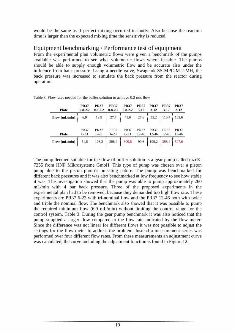
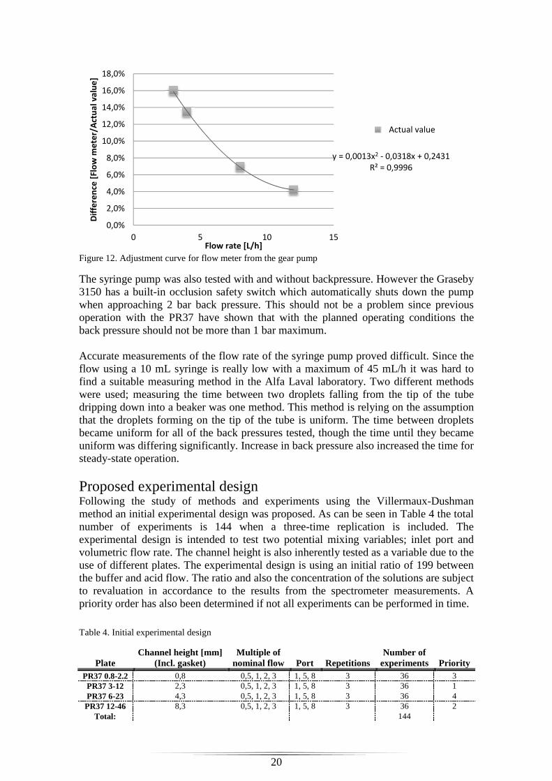
The pump deemed suitable for the flow of buffer solution is a gear pump called mzr®-7255 from HNP Mikrosysteme GmbH. This type of pump was chosen over a piston pump due to the piston pump’s pulsating nature. The pump was benchmarked for different back pressures and it was also benchmarked at low frequency to see how stable it was. The investigation showed that the pump was able to pump approximately 260 mL/min with 4 bar back pressure. Three of the proposed experiments in the experimental plan had to be removed, because they demanded too high flow rate. These experiments are PR37 6-23 with tri-nominal flow and the PR37 12-46 both with twice and triple the nominal flow. The benchmark also showed that it was possible to pump the required minimum flow (6.9 mL/min) without limiting the control range for the control system, Table 3. During the gear pump benchmark it was also noticed that the pump supplied a larger flow compared to the flow rate indicated by the flow meter. Since the difference was not linear for different flows it was not possible to adjust the settings for the flow meter to address the problem. Instead a measurement series was performed over four different flow rates. From these measurements an adjustment curve was calculated, the curve including the adjustment function is found in Figure 12.

20

Figure 12. Adjustment curve for flow meter from the gear pump

The syringe pump was also tested with and without backpressure. However the Graseby 3150 has a built-in occlusion safety switch which automatically shuts down the pump when approaching 2 bar back pressure. This should not be a problem since previous operation with the PR37 have shown that with the planned operating conditions the back pressure should not be more than 1 bar maximum. Accurate measurements of the flow rate of the syringe pump proved difficult. Since the flow using a 10 mL syringe is really low with a maximum of 45 mL/h it was hard to find a suitable measuring method in the Alfa Laval laboratory. Two different methods were used; measuring the time between two droplets falling from the tip of the tube dripping down into a beaker was one method. This method is relying on the assumption that the droplets forming on the tip of the tube is uniform. The time between droplets became uniform for all of the back pressures tested, though the time until they became uniform was differing significantly. Increase in back pressure also increased the time for steady-state operation.

Proposed experimental design Following the study of methods and experiments using the Villermaux-Dushman method an initial experimental design was proposed. As can be seen in Table 4 the total number of experiments is 144 when a three-time replication is included. The experimental design is intended to test two potential mixing variables; inlet port and volumetric flow rate. The channel height is also inherently tested as a variable due to the use of different plates. The experimental design is using an initial ratio of 199 between the buffer and acid flow. The ratio and also the concentration of the solutions are subject to revaluation in accordance to the results from the spectrometer measurements. A priority order has also been determined if not all experiments can be performed in time.

Table 4. Initial experimental design

Plate Channel height [mm]

(Incl. gasket) Multiple of

nominal flow Port Repetitions Number of

experiments Priority PR37 0.8-2.2 0,8 0,5, 1, 2, 3 1, 5, 8 3 36 3 PR37 3-12 2,3 0,5, 1, 2, 3 1, 5, 8 3 36 1 PR37 6-23 4,3 0,5, 1, 2, 3 1, 5, 8 3 36 4 PR37 12-46 8,3 0,5, 1, 2, 3 1, 5, 8 3 36 2

Total:

144

y = 0,0013x2 - 0,0318x + 0,2431

R² = 0,9996

0,0%

2,0%

4,0%

6,0%

8,0%

10,0%

12,0%

14,0%

16,0%

18,0%

0 5 10 15

Dif

fere

nce

[F

low

me

ter/

Act

ua

l v

alu

e]

Flow rate [L/h]

Actual value

21

In order to yield results which are comparable the proposed experiments are having the same axial velocity, for the nominal flow, for all the plates. The axial velocity is set to 0.2 m/s, this value is similar to the de facto value used by Alfa Laval Reactor technology department. The flow rate they use as nominal flow is supposed to have the axial velocity of 0.3 m/s, but the calculations in this project shows that the actual axial velocity is approximately 0.2 m/s for all but the smallest plate, PR37 0.8-2.2, where the velocity is close to 0.3 m/s. This difference is due to the changes in design and especially the design of the process gasket. See Appendix D for more details of the calculations. Table 5. Linear velocities using the general flow rates

Plate PR37 0.8-

2.2 PR37 3-

12 PR37 6-

23 PR37 12-

46

Nominal Flow [L/min] 0,02 0,05 0,1 0,2

Channel Height incl. gasket [m] 8,0E-04 2,3E-03 4,3E-03 8,3E-03

Maximum linear velocity

Min. Channel Cross sectional area [m2]

8,5E-07 3,0E-06 6,0E-06 1,2E-05

Min. Width [m] 1,1E-03 1,5E-03 1,5E-03 1,5E-03 Hydraulic diameter [m] 9,1E-04 1,8E-03 2,2E-03 2,5E-03

Maximum Linear velocity [m/s] 0,392 0,242 0,258 0,268

Minimum linear velocity

Max. Channel Cross sectional area [m2]

1,8E-06 6,0E-06 1,2E-05 2,4E-05

Max. Width [m] 2,3E-03 3,0E-03 3,0E-03 3,0E-03 Hydraulic diameter [m] 1,2E-03 2,6E-03 3,5E-03 4,4E-03

Minimum Linear velocity [m/s] 0,185 0,121 0,129 0,134

Mean Linear velocity [m/s] 0,289 0,181 0,194 0,200

Tailoring reaction rates As an axial length it was decided that 30 cm was suitable to be the reaction length. This length infers that approximately 10% of the total reactor is used for the characterization as can be seen in Table 6. When the flow rate is changed the reaction rate inevitably must be changed accordingly in order to keep the reaction length constant. Table 6 shows that the four different flow rates yield four corresponding desired reaction times. Table 6. Used volume and length for reactor characterization

Plate name Flow rate (ml/min)

Reaction Length (m)

Reaction time (s)

Reaction volume (ml)

Utilized % of Reactor

PR37 0.8-2.2 6,9283 0,3 3 0,346 9,82%

PR37 0.8-2.2 13,8566 0,3 1,5 0,346 9,82%

PR37 0.8-2.2 27,7132 0,3 0,75 0,346 9,82%

PR37 0.8-2.2 41,5698 0,3 0,50 0,346 9,82%

PR37 3-12 27,6 0,3 3 1,38 10,18%

PR37 3-12 55,2 0,3 1,5 1,38 10,18%

PR37 3-12 110,4 0,3 0,75 1,38 10,18%

PR37 3-12 165,6 0,3 0,50 1,38 10,18%

PR37 6-23 51,6 0,3 3 2,58 10,37%

PR37 6-23 103,2 0,3 1,5 2,58 10,37%

PR37 6-23 206,4 0,3 0,75 2,58 10,37%

PR37 12-46 99,6 0,3 3 4,98 10,44%

PR37 12-46 199,2 0,3 1,5 4,98 10,44%

22

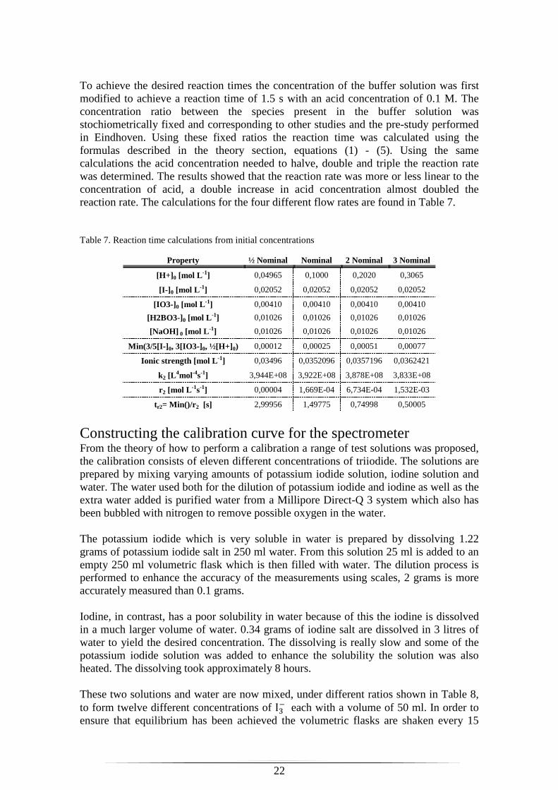
To achieve the desired reaction times the concentration of the buffer solution was first modified to achieve a reaction time of 1.5 s with an acid concentration of 0.1 M. The concentration ratio between the species present in the buffer solution was stochiometrically fixed and corresponding to other studies and the pre-study performed in Eindhoven. Using these fixed ratios the reaction time was calculated using the formulas described in the theory section, equations (1) - (5). Using the same calculations the acid concentration needed to halve, double and triple the reaction rate was determined. The results showed that the reaction rate was more or less linear to the concentration of acid, a double increase in acid concentration almost doubled the reaction rate. The calculations for the four different flow rates are found in Table 7. Table 7. Reaction time calculations from initial concentrations

Property ½ Nominal Nominal 2 Nominal 3 Nominal

[H+] 0 [mol L -1] 0,04965 0,1000 0,2020 0,3065

[I-] 0 [mol L -1] 0,02052 0,02052 0,02052 0,02052

[IO3-] 0 [mol L -1] 0,00410 0,00410 0,00410 0,00410

[H2BO3-]0 [mol L -1] 0,01026 0,01026 0,01026 0,01026

[NaOH] 0 [mol L -1] 0,01026 0,01026 0,01026 0,01026

Min(3/5[I-] 0, 3[IO3-]0, ½[H+]0) 0,00012 0,00025 0,00051 0,00077

Ionic strength [mol L -1] 0,03496 0,0352096 0,0357196 0,0362421

k2 [L4mol-4s-1] 3,944E+08 3,922E+08 3,878E+08 3,833E+08

r2 [mol L -1s-1] 0,00004 1,669E-04 6,734E-04 1,532E-03

tr2= Min()/r 2 [s] 2,99956 1,49775 0,74998 0,50005

Constructing the calibration curve for the spectrometer From the theory of how to perform a calibration a range of test solutions was proposed, the calibration consists of eleven different concentrations of triiodide. The solutions are prepared by mixing varying amounts of potassium iodide solution, iodine solution and water. The water used both for the dilution of potassium iodide and iodine as well as the extra water added is purified water from a Millipore Direct-Q 3 system which also has been bubbled with nitrogen to remove possible oxygen in the water. The potassium iodide which is very soluble in water is prepared by dissolving 1.22 grams of potassium iodide salt in 250 ml water. From this solution 25 ml is added to an empty 250 ml volumetric flask which is then filled with water. The dilution process is performed to enhance the accuracy of the measurements using scales, 2 grams is more accurately measured than 0.1 grams. Iodine, in contrast, has a poor solubility in water because of this the iodine is dissolved in a much larger volume of water. 0.34 grams of iodine salt are dissolved in 3 litres of water to yield the desired concentration. The dissolving is really slow and some of the potassium iodide solution was added to enhance the solubility the solution was also heated. The dissolving took approximately 8 hours. These two solutions and water are now mixed, under different ratios shown in Table 8, to form twelve different concentrations of I � each with a volume of 50 ml. In order to ensure that equilibrium has been achieved the volumetric flasks are shaken every 15

23

minutes for three hours. It is important that equilibrium has been achieved otherwise equation (6) is not valid. The concentration of I �is calculated using equations (18) and (19). This concentration of triiodide is now paired with the absorbance acquired from the spectrometer for the respective concentrations, column 4 and 5 in Table 8. Table 8. Mixing table and absorbance results for calibration curve

Volume of KI-solution [mL]

Volume of I2-solution [mL]

Volume of added water[mL]

Concentration of ��[mole/L] Absorbance

10 10 80 9,26E-06 0,070

20 10 70 1,49E-05 0,156

30 10 60 1,89E-05 0,183

10 40 50 3,99E-05 0,359

20 40 40 6,08E-05 0,533

30 40 30 7,61E-05 0,684

10 70 20 7,41E-05 0,604

20 70 10 1,08E-04 0,932

30 70 0 1,25E-04 0,090

In order to achieve the calibration curve the absorbance is plotted against the triiodide concentration. The graph can be found in Figure 13. As long as the absorbance has a linear correlation with the concentration the Lambert-Beer law is valid, it is this range we are interested and especially the slope of this linear relation. Using the curve fitting toolbox in MatLab® the slope of the curve is determined to 9826 L/mol. Also knowing the measuring length of the flow cell the molar extinction coefficient can be determined and used for other types of flow cells using the same spectrometer.

Figure 13. Calibration curve

For the purpose of the current project the slope value including flow cell is used since the same equipment will be used for the entire experiment series. The expression for calculating concentration of triiodide from absorbance is shown in equation (27). The linear regression was performed with the two points with the highest concentration as outliers.

�� = � ¡¢£�¤ , (27)

where abs is the absorbance measured and cI3 is the triiodide concentration in mol/l.

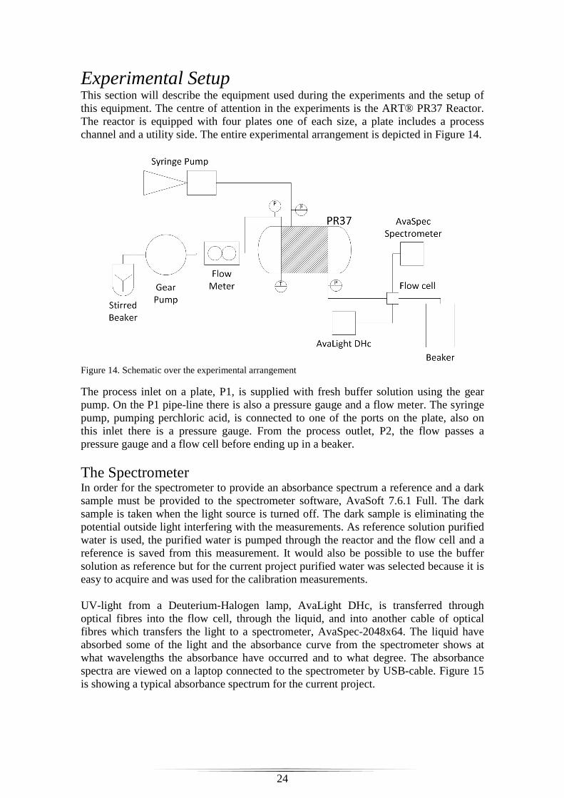
24

Experimental Setup This section will describe the equipment used during the experiments and the setup of this equipment. The centre of attention in the experiments is the ART® PR37 Reactor. The reactor is equipped with four plates one of each size, a plate includes a process channel and a utility side. The entire experimental arrangement is depicted in Figure 14.

Figure 14. Schematic over the experimental arrangement

The process inlet on a plate, P1, is supplied with fresh buffer solution using the gear pump. On the P1 pipe-line there is also a pressure gauge and a flow meter. The syringe pump, pumping perchloric acid, is connected to one of the ports on the plate, also on this inlet there is a pressure gauge. From the process outlet, P2, the flow passes a pressure gauge and a flow cell before ending up in a beaker.

The Spectrometer In order for the spectrometer to provide an absorbance spectrum a reference and a dark sample must be provided to the spectrometer software, AvaSoft 7.6.1 Full. The dark sample is taken when the light source is turned off. The dark sample is eliminating the potential outside light interfering with the measurements. As reference solution purified water is used, the purified water is pumped through the reactor and the flow cell and a reference is saved from this measurement. It would also be possible to use the buffer solution as reference but for the current project purified water was selected because it is easy to acquire and was used for the calibration measurements. UV-light from a Deuterium-Halogen lamp, AvaLight DHc, is transferred through optical fibres into the flow cell, through the liquid, and into another cable of optical fibres which transfers the light to a spectrometer, AvaSpec-2048x64. The liquid have absorbed some of the light and the absorbance curve from the spectrometer shows at what wavelengths the absorbance have occurred and to what degree. The absorbance spectra are viewed on a laptop connected to the spectrometer by USB-cable. Figure 15 is showing a typical absorbance spectrum for the current project.

25

Figure 15. Typical absorbance spectrum for the iodide-iodate method

During the first experiments there was problem in yielding data. Because the flow cell was initially mounted in a horizontal position there was a possibility that the flow was not large enough to entirely fill the flow cell resulting in air pockets disturbing the measurements. A small rebuild where the flow cell was positioned in a vertical state instead provided better data and clear tops in the absorbance spectra was observed. The tops were also corresponding to the expected wavelengths of 288 nm and 353 nm for triiodide ions and 248 nm for the iodide ion. The other species present in the buffer has absorbance outside the scope of the current spectrometer. Because there is less interference from other species at 353 nm this wavelength is used to measure the triiodide concentration. Using the calibration described earlier the absorbance can be converted into a concentration of� �. As described in the theory section the segregation index can be calculated when the triiodide concentration is known. The buffer solution for the experiments is of the same concentration for all experiments, the concentrations are presented in Table 7. These concentrations translate into a mass of each species to be added for each litre of buffer solution. Using the preparation scheme described in Appendix A the buffer solution was prepared, usually in batches of three litres. Preparation of the perchloric acid is performed using the instructions found in Appendix A. Depending on the flow rate the acid concentration has to be adjusted accordingly, as shown in Table 7.

Limitations and time restrictions When trying to perform the different experiments problem with too high pressure for certain flow rates occurred. This problem was indicated in the form that the occlusion safety feature on the syringe pump was activated and the pump shutdown automatically. Therefore the experiments with threefold nominal flow were deemed impossible to perform and cut from the experimental plan. Also for the smallest plate the pressure limitation applied to the flow rate of twice the nominal. For the experiments a number of chemicals were needed. Most of these were easy to acquire and had no limitation for use within Alfa Laval, however with boric acid this

26

was not the case. The procedure for getting approval to purchase and use boric acid dragged on for weeks and the available time for experiments was drastically decreased. In the light of this it was decided to limit the experimental plan further. This was done by cutting the PR37 6-23 plate experiments and also cutting the port 5 experiments. In addition the comparison of port 1 and 2 was only performed for the PR37 3-12 plate for these ports the use of a nozzle was also investigated. The use of nozzle was not included in the first experimental plan but was added now since it is a highly interesting variable and also the implementation in the experiments is quite easy and fast compared to shifting between plates. As described a number of experiments were cut from the experimental design and the experiments performed are listed in Table 9. Table 9. The performed experiments during the project

Plate name Plate depth Excl. gasket Port Nozzle

Flow rate Actual/Nominal

Maximum Reynolds

PR37 0.8-2.2 0,5 mm 1 No 0,5 139 PR37 0.8-2.2 0,5 mm 1 No 1 278 PR37 3-12 2 mm 1 No 0,5 276 PR37 3-12 2 mm 1 No 1 553 PR37 3-12 2 mm 1 No 2 1105 PR37 3-12 2 mm 2 No 0,5 276 PR37 3-12 2 mm 2 No 1 553 PR37 3-12 2 mm 2 No 2 1105 PR37 3-12 2 mm 1 100 µm 0,5 276 PR37 3-12 2 mm 1 100 µm 1 553 PR37 3-12 2 mm 1 100 µm 2 1105 PR37 3-12 2 mm 2 100 µm 0,5 276 PR37 3-12 2 mm 2 100 µm 1 553 PR37 3-12 2 mm 2 100 µm 2 1105 PR37 12-46 8 mm 1 No 0,5 387 PR37 12-46 8 mm 1 No 1 773

The use of nozzle Using a nozzle with a diameter of 100 microns will significantly increase the axial velocity of the acid flow. The axial flow velocity is increased by 289 times (100 times for the PR37 0.8-2.2). As can be seen in Table 10 the velocity ratio between the buffer solution and the acid solution is drastically changed with the use of the nozzle. This should increase the mixing of the fluids at the inlet. Table 10. Change in inlet velocity when using nozzle.

Type of inlet Plate Flow ratio Inlet diameters [m] Flow m3/s Velocity [m/s] Buffer/Acid

Velocity ratio

Port PR37 0.8-2.2 0,5 0,001 7,9E-07 0,00074 272,07 Nozzle PR37 0.8-2.2 0,5 0,0001 5,8E-10 0,07351 2,72

Port PR37 0.8-2.2 1 0,0017 1,2E-09 0,00051 393,14 Nozzle PR37 0.8-2.2 1 0,0001 1,2E-09 0,14702 1,36

Port PR37 3-12 0,5 0,0017 2,3E-09 0,00101 197,37 Nozzle PR37 3-12 0,5 0,0001 2,3E-09 0,29285 0,68

Port PR37 3-12 1 0,0017 4,6E-09 0,00203 98,69 Nozzle PR37 3-12 1 0,0001 4,6E-09 0,58569 0,34


Port PR37 12-46 0,5 0,0017 8,3E-09 0,00366 54,69 Nozzle PR37 12-46 0,5 0,0001 8,3E-09 1,05679 0,19


27

Data acquisition The pressure gauges, thermo element and flow meter are connected to a RMS-system, remote monitoring system. The RMS system is then connected to a desktop PC through USB cables, the signals are treated in the PC using a program called LabVIEW®, developed by National Instruments. Within the LabVIEW environment it is possible to log the data from the different instruments. The logging is started manually and produces a text file with tab-separated columns, one column for each input and also columns for timestamp and error messages. The data log files are after minor modification easily read by MatLab using the tdfread-function. The software for the spectrometer, AvaSoft 7.6.1 Full, has a built in function which logs the specified data, up to 8 different sets, to excel-files. During this experiment three different data sets were logged during the experiments; absorbance at 353 nm, complete absorbance spectrum and complete scope spectrum. The scope spectrum is an indication of how dense the solution is compared to the maximum capability of the spectrometer and software. In MatLab the excel files are easily imported using the xlsread-function. A basic instruction of how the spectrometer software is operated for the current project is found in Appendix C.

28

Results When all data has been imported into MatLab the data transformation can begin. The different data log files are investigated and the uninteresting data in the beginning and end is removed, i.e. the data before steady-state has been achieved. The absorbance graphs are found in Appendix F. The data treatment revealed that some of the experimental runs have yielded data which is vastly different from other experiments using the same setup, in these cases the data series with the differing result has been removed. Figure 16 illustrates one of these vastly differing absorbance results. The occurrence of these results is discussed further in the discussion section.

Figure 16. An example of vastly differing absorbance result

The incomparable parameters Through the concentration of triiodide the absorbance spectrum and segregation index are connected, the absorbance is needed to calculate the concentration of triiodide and thereby also the segregation index. Both these parameters are qualitative parameters meaning that they are not directly comparable between the different systems of concentrations and flow rates.

Absorbance The absorbance data is adjusted to only include the steady-state data and is then averaged over time. The absorbance measured for the different experiments is listed in Table 11. Table 11. Absorbance data from the experiments

Plate name Plate depth Excl. gasket Port

Flow rate Actual/Nominal

Replications

Average abs #1 #2 #3 #4

PR37 0.8-2.2 0,5 mm 1 0,5 0,059 0,052

0,056 PR37 0.8-2.2 0,5 mm 1 1 0,143 0,121 0,163 0,138 0,141 PR37 3-12 2 mm 1 0,5 0,218 0,209 0,220 - 0,216 PR37 3-12 2 mm 1 1 0,463 0,467 0,402 0,481 0,453 PR37 3-12 2 mm 1 2 0,760 0,767 0,792 - 0,773 PR37 3-12 2 mm 2 0,5 0,203 0,236 0,243 - 0,227 PR37 3-12 2 mm 2 1 0,389 0,356 0,471 0,481 0,424 PR37 3-12 2 mm 2 2 0,766 0,787 0,813 - 0,788 PR37 3-12 2 mm 1 - Nozzle 0,5 0,243 0,273 - - 0,258 PR37 3-12 2 mm 1 - Nozzle 1 0,093 0,109 - - 0,101 PR37 3-12 2 mm 1 - Nozzle 2 0,574 - - - 0,574 PR37 3-12 2 mm 2 - Nozzle 0,5 0,159 0,180 - - 0,169 PR37 3-12 2 mm 2 - Nozzle 1 0,330 0,350 - - 0,340 PR37 3-12 2 mm 2 - Nozzle 2 0,658 - - - 0,658 PR37 12-46 8 mm 1 0,5 0,258 0,268 0,302 - 0,276 PR37 12-46 8 mm 1 1 0,478 0,438 0,452 - 0,456

29

The absorbance data is not a suitable parameter for comparing the different plates and flow rates since the concentrations and flows differ, the absorbance has to be converted further. Comparing the absorbance to the calibration curve and the validity of the Lambert-Beer law it should be noted that the absorbance for experiments using twice the nominal flow is on the border of the validity for the Lambert-Beer law. The use of the Lambert-Beer estimation for absorbance exceeding its validity will overestimate the concentration hence overestimate the mixing time.

Segregation index The calculation of the segregation index is quite straight forward from what is described in the theory section. Using the logged data and equations (6), (13), (16) and (27) the segregation index is calculated. As can be seen in Figure 17 the results within each experimental run are a bit fluctuating. The setups which vary the most are varying ±15% however the majority of the results are within ±5% from the averaged value.

Figure 17. Measurement of the fluctuations within measurements of segregation index

Micromixing model The micromixing model chosen for the current project is the so called incorporation model. The reason is that this model is suitable for plug-flow environments and also simple to implement. Using the model a graph showing segregation index as a function of mixing time can be produced. The MatLab-code compiled for these calculations is included in Appendix G. The MatLab-code is basically solving the mass balance for a number of incorporation times, which for the incorporation model is equal to mixing time, each one is resulting in a segregation index. Solving the mass balance for a sufficiently large number of incorporation times yields a curve showing the relation between segregation index and mixing time. The appearance of that curve is dependent upon the flow rates and species concentration in the system which is why it has to be calculated for every type of system used in the project. Because of that the MatLab-script is compiled with four inlet variables; buffer flow rate, acid flow rate, acid concentration and segregation index. The segregation index is used to draw a straight line at the desired segregation index and facilitates a rapid determination of mixing time. The equation system which is solved in the end of the MatLab-script is the derivative of the concentration for each of the species, solving this system of equations for a specific range of mixing times yields a concentration vector from which a segregation index is calculated.

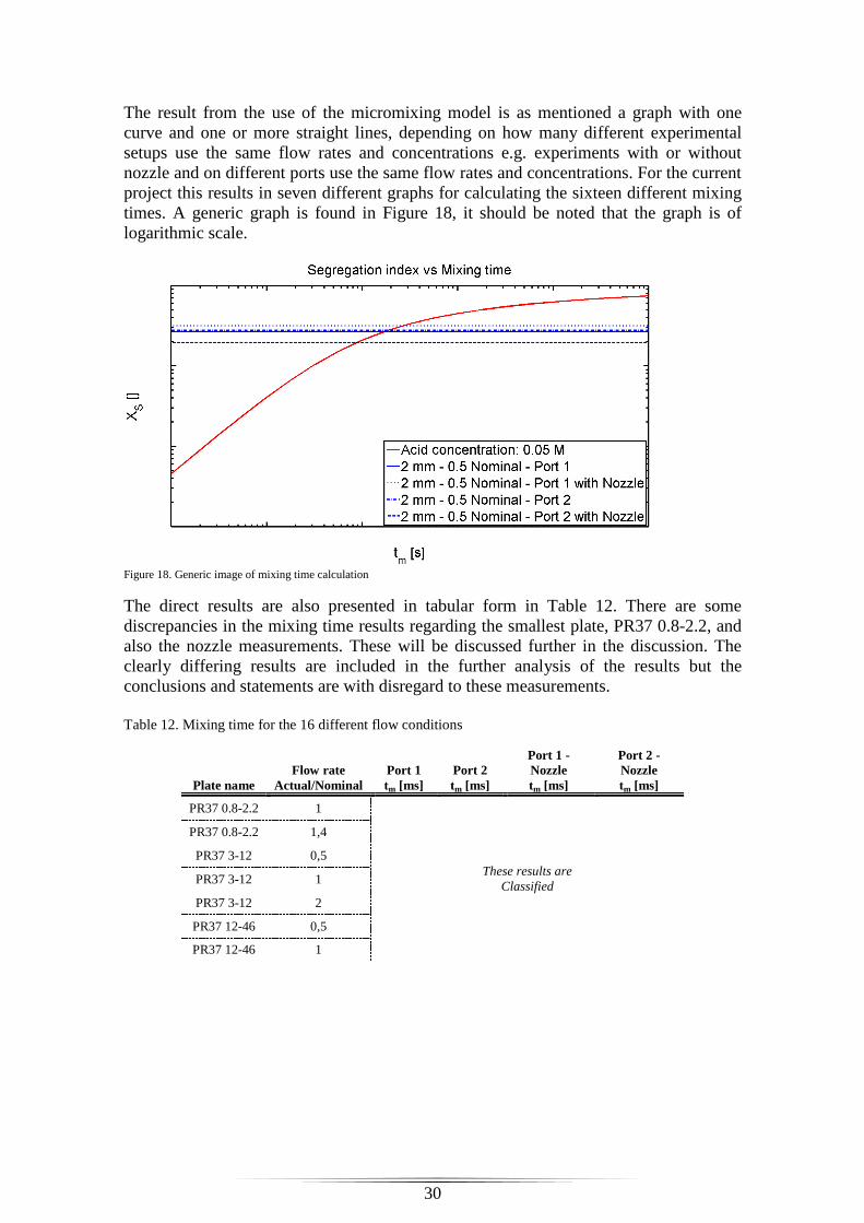
30

The result from the use of the micromixing model is as mentioned a graph with one curve and one or more straight lines, depending on how many different experimental setups use the same flow rates and concentrations e.g. experiments with or without nozzle and on different ports use the same flow rates and concentrations. For the current project this results in seven different graphs for calculating the sixteen different mixing times. A generic graph is found in Figure 18, it should be noted that the graph is of logarithmic scale.

Figure 18. Generic image of mixing time calculation

The direct results are also presented in tabular form in Table 12. There are some discrepancies in the mixing time results regarding the smallest plate, PR37 0.8-2.2, and also the nozzle measurements. These will be discussed further in the discussion. The clearly differing results are included in the further analysis of the results but the conclusions and statements are with disregard to these measurements. Table 12. Mixing time for the 16 different flow conditions

Plate name Flow rate

Actual/Nominal Port 1 tm [ms]

Port 2 tm [ms]

Port 1 - Nozzle tm [ms]

Port 2 - Nozzle tm [ms]

PR37 0.8-2.2 1

These results are Classified

PR37 0.8-2.2 1,4

PR37 3-12 0,5

PR37 3-12 1

PR37 3-12 2

PR37 12-46 0,5

PR37 12-46 1

31

Figure 19. Mixing time vs. pressure drop, Main in -Main Out

Figure 20. Mixing time vs. pressure drop, Acid in - Main Out

From Figure 19 and Figure 20 it can be seen that there is not much difference in the pressure between the inlets. It can also be seen that for the different types of flow rates, used ports and nozzles the trend is that the mixing time is decreasing with higher pressure drop. The effect of the increased pressure drop varies though. The mixing time is a direct measure of how fast the mixing is at the current conditions. In order to characterize the reactor the mixing time is compared to relevant parameters. For micromixers in general a comparative analysis has been performed by Falk and Commenge, (Falk and Commenge, 2010) the main parameters they compare reactors/mixers by is Reynolds number and energy dissipation. Energy dissipation is a measure of how large the pump effect is compared to the mixing performance, the classic “bang for the buck”-comparison. The Reynolds comparison sheet has also what you could call a normalised mixing time, the mixing time is normalised by the characteristic diameter of the reactor. This normalisation means that a reactor can be compensated for a bit longer mixing time by having a larger diameter. Figure 21 and Figure 22 shows these comparison parameters for the different plates with the inlet at port 1 and no nozzle used.

Figure 21. Normalised mixing time versus Reynolds number, Port 1.

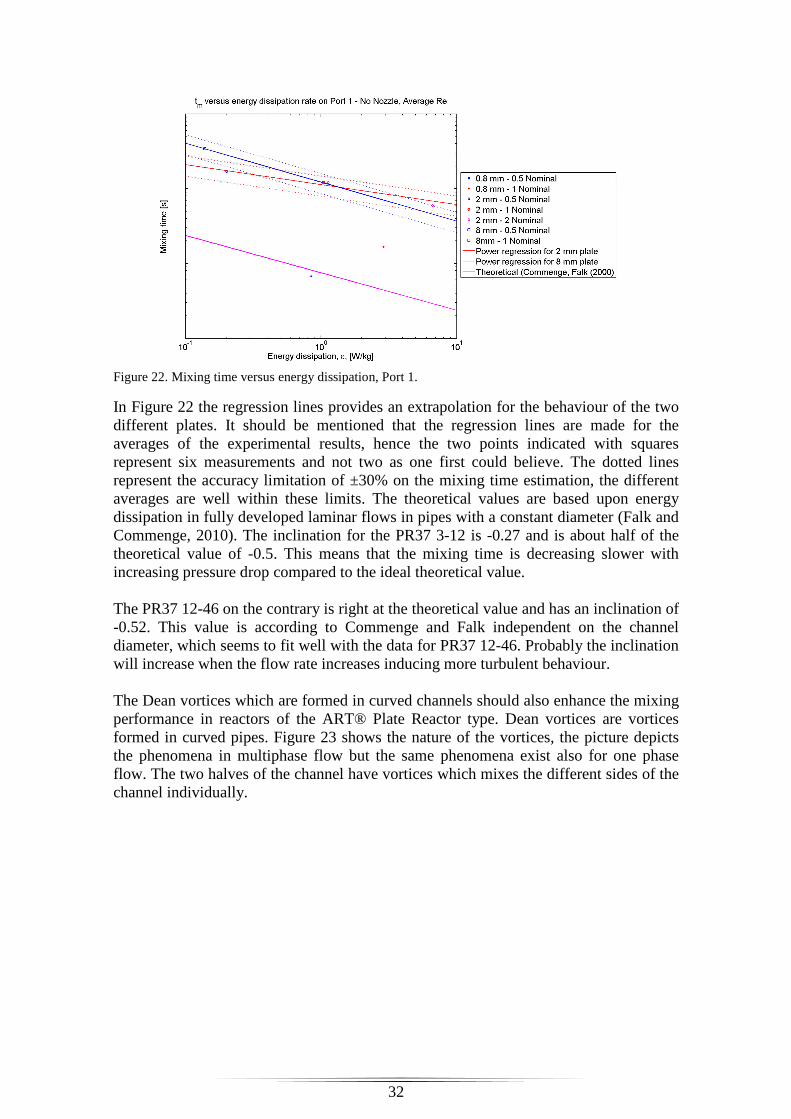
32

Figure 22. Mixing time versus energy dissipation, Port 1.

In Figure 22 the regression lines provides an extrapolation for the behaviour of the two different plates. It should be mentioned that the regression lines are made for the averages of the experimental results, hence the two points indicated with squares represent six measurements and not two as one first could believe. The dotted lines represent the accuracy limitation of ±30% on the mixing time estimation, the different averages are well within these limits. The theoretical values are based upon energy dissipation in fully developed laminar flows in pipes with a constant diameter (Falk and Commenge, 2010). The inclination for the PR37 3-12 is -0.27 and is about half of the theoretical value of -0.5. This means that the mixing time is decreasing slower with increasing pressure drop compared to the ideal theoretical value. The PR37 12-46 on the contrary is right at the theoretical value and has an inclination of -0.52. This value is according to Commenge and Falk independent on the channel diameter, which seems to fit well with the data for PR37 12-46. Probably the inclination will increase when the flow rate increases inducing more turbulent behaviour. The Dean vortices which are formed in curved channels should also enhance the mixing performance in reactors of the ART® Plate Reactor type. Dean vortices are vortices formed in curved pipes. Figure 23 shows the nature of the vortices, the picture depicts the phenomena in multiphase flow but the same phenomena exist also for one phase flow. The two halves of the channel have vortices which mixes the different sides of the channel individually.

33

Figure 23. Sketch of Dean vortices, picture from Palo Alto Research Center.

Figure 24. Power regression curves and theoretical trend curves; inverse diffusion coefficients vs. Reynolds number

Figure 24 shows the power regression curves for the other parameter comparison. Using these comparisons the experimental results are much closer to the theoretical literature values. The PR37 3-12 also here has a slightly lower inclination compared to the theoretical value for laminar flow, -0.67 and -1 respectively. For the PR37 12-46 the slope is almost identical to the theoretical value for turbulent flows, indicating turbulent behaviour at Reynolds numbers traditionally associated with laminar flows.

Inside wall

Outside wall

34

Figure 25. Inverse diffusion coefficient versus Reynolds for PR37 3-12 plate.

Although all the data for the experiments performed using a nozzle is not consistent it is possible to make an estimation of the average tendency. The inclination results for the nozzle are only to illustrate the large effect the nozzle has on micromixing overall, it should not be taken as a true value. It is interesting though to see the very similar trend for the two non-nozzle and the two nozzle experiments respectively, Figure 25.

35

Discussion In the discussion chapter the results will be discussed in the terms of reliability and reproducibility. The results will also be compared to previous studies of micromixing and mixing time, especially to the comprehensive comparison performed by Falk and Commenge, (Falk and Commenge, 2010). In the end it will also be discussed how this investigation can be extended and what improvements and changes are recommended.

Reliability & Reproducibility The very most part of the results extracted from the spectrometer software was consistent at least within a ±10% margin and most of them within ±5%. Having literature studies stating that an accuracy of more than ±30% is hard to achieve for the final results the reproducibility in these experiments are good. There have been some results which has differed a very large amount, >±100%, from previous measurements. The syringe pump is thought to be the source to these strange readings. In the total experimental system there are two moving parts, the gear pump and the syringe pump, and two solutions, buffer solution and acid solution. These four variables are the only variables in the system, if the spectrometer is assumed to have constant performance. Since the strange results seem to be occurring randomly and inconsistently, i.e. the same measurement with the same buffer and acid can occasionally produce these outliers in result, the syringe pump is believed to be the source. The gear pumps flow rate is monitored with a flow meter, however this was not possible to do with the syringe pump. As described in the report the syringe pump was benchmarked and seemed to be able to have a constant and accurate flow rate, but quite possibly it sometimes produces these faulty flow rates which are the reason for the strange absorbance readings. It has been noted that the inconsistencies in the absorbance measurements could be related to the pressure in the reactor during the experiment, a high pressure resulting in less accurate flow rate from the syringe pump. A few of the experiments, the ones with twice the nominal flow for PR37 3-12, is on the limit of where the Lambert-Beer law is valid. If not within the limit the use of the Lambert-Beer approximation will overestimate the concentration and also the mixing time. The design of the syringe pump is also the reason to a number of experimental setups being cut. The syringe pumps built in occlusion safety disengages the pump for a number of experiments.

PR37 0.8-2.2 plate Some of the results from the absorbance measurements are confusing these results are some of the measurements with nozzle and the measurement on the PR37 0.8-2.2 plate. The tests on the PR37 0.8-2.2 plate was hard to perform since there was problem with some occlusion in the syringe pump. Also the gear pump delivered a much higher flow rate compared to the indicated flow rate of the flow meter, more than 100% more. The experiments on the PR37 0.8-2.2 plate is also operating on a higher pressure, 0.27 and 0.44 bar, compared to the 2mm ones with the same ratio of nominal flow rate, 0,09 and 0,2 bar. The pressure drop should indicate that the mixing when using nominal flow should be higher than for the half nominal flow setup. But the results indicate otherwise. A potential explanation is that the flow rates are very low for the gear pump and as

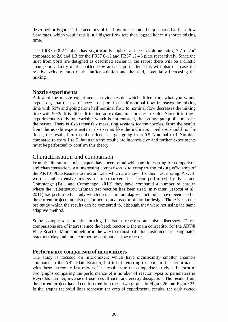
36

described in Figure 12 the accuracy of the flow meter could be questioned at these low flow rates, which would result in a higher flow rate than logged hence a shorter mixing time. The PR37 0.8-2.2 plate has significantly higher surface-to-volume ratio, 3.7 m2/m3 compared to 2.0 and 1.3 for the PR37 6-12 and PR37 12-46 plate respectively. Since the inlet from ports are designed as described earlier in the report there will be a drastic change in velocity of the buffer flow at each port inlet. This will also decrease the relative velocity ratio of the buffer solution and the acid, potentially increasing the mixing.

Nozzle experiments A few of the nozzle experiments provide results which differ from what you would expect e.g. that the use of nozzle on port 1 at half nominal flow increases the mixing time with 50% and going from half nominal flow to nominal flow decreases the mixing time with 90%. It is difficult to find an explanation for these results. Since it in these experiments is only one variable which is not constant, the syringe pump, this must be the reason. There is also rather few measuring sessions for the nozzles. From the results from the nozzle experiments it also seems like the inclination perhaps should not be linear, the results hint that the effect is larger going from 0.5 Nominal to 1 Nominal compared to from 1 to 2, but again the results are inconclusive and further experiments must be performed to confirm this theory.

Characterisation and comparison From the literature studies papers have been found which are interesting for comparison and characterisation. An interesting comparison is to compare the mixing efficiency of the ART® Plate Reactor to micromixers which are known for their fast mixing. A well-written and extensive review of micromixers has been performed by Falk and Commenge (Falk and Commenge, 2010) they have compared a number of studies where the Villermaux/Dushman test reaction has been used. In Nantes (Habchi et al., 2011) has performed a study which uses a similar adaptive method as have been used in the current project and also performed it on a reactor of similar design. There is also the pre-study which the results can be compared to, although they were not using the same adaptive method. Some comparisons to the mixing in batch reactors are also discussed. These comparisons are of interest since the batch reactor is the main competitor for the ART® Plate Reactor. Main competitor in the way that most potential customers are using batch reactors today and not a competing continuous flow reactor.

Performance comparison of micromixers The study is focused on micromixers which have significantly smaller channels compared to the ART Plate Reactor, but it is interesting to compare the performance with these extremely fast mixers. The result from the comparison study is in form of two graphs comparing the performance of a number of reactor types to parameters as Reynolds number, inverse diffusion coefficient and energy dissipation. The results from the current project have been inserted into these two graphs in Figure 26 and Figure 27. In the graphs the solid lines represent the area of experimental results, the dash-dotted

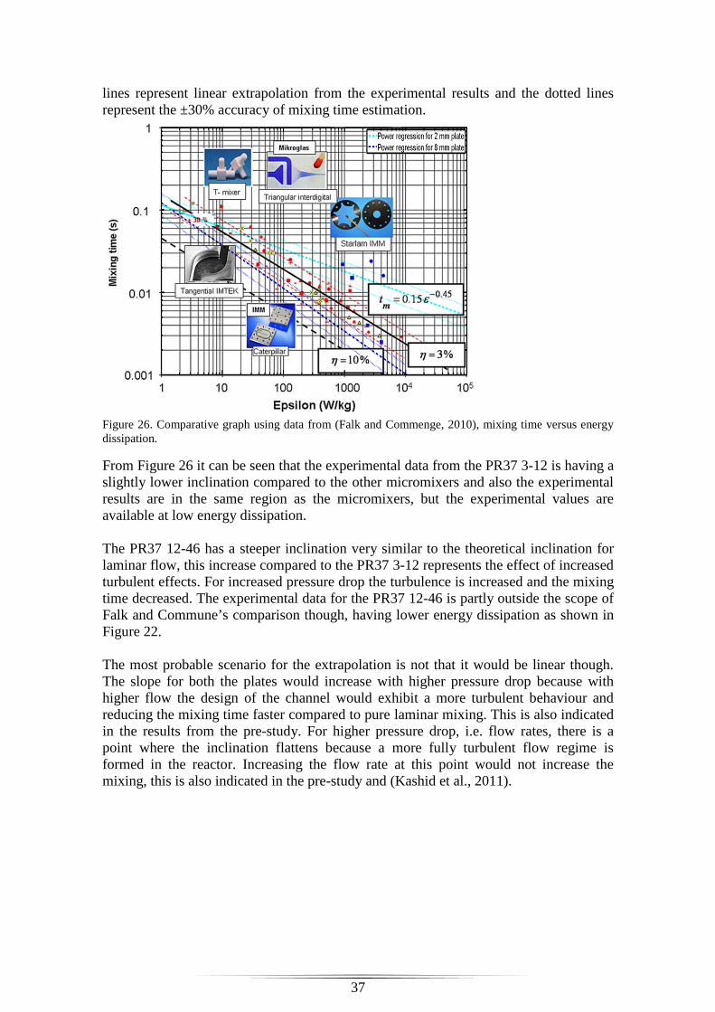
37

lines represent linear extrapolation from the experimental results and the dotted lines represent the ±30% accuracy of mixing time estimation.

Figure 26. Comparative graph using data from (Falk and Commenge, 2010), mixing time versus energy dissipation.

From Figure 26 it can be seen that the experimental data from the PR37 3-12 is having a slightly lower inclination compared to the other micromixers and also the experimental results are in the same region as the micromixers, but the experimental values are available at low energy dissipation. The PR37 12-46 has a steeper inclination very similar to the theoretical inclination for laminar flow, this increase compared to the PR37 3-12 represents the effect of increased turbulent effects. For increased pressure drop the turbulence is increased and the mixing time decreased. The experimental data for the PR37 12-46 is partly outside the scope of Falk and Commune’s comparison though, having lower energy dissipation as shown in Figure 22. The most probable scenario for the extrapolation is not that it would be linear though. The slope for both the plates would increase with higher pressure drop because with higher flow the design of the channel would exhibit a more turbulent behaviour and reducing the mixing time faster compared to pure laminar mixing. This is also indicated in the results from the pre-study. For higher pressure drop, i.e. flow rates, there is a point where the inclination flattens because a more fully turbulent flow regime is formed in the reactor. Increasing the flow rate at this point would not increase the mixing, this is also indicated in the pre-study and (Kashid et al., 2011).

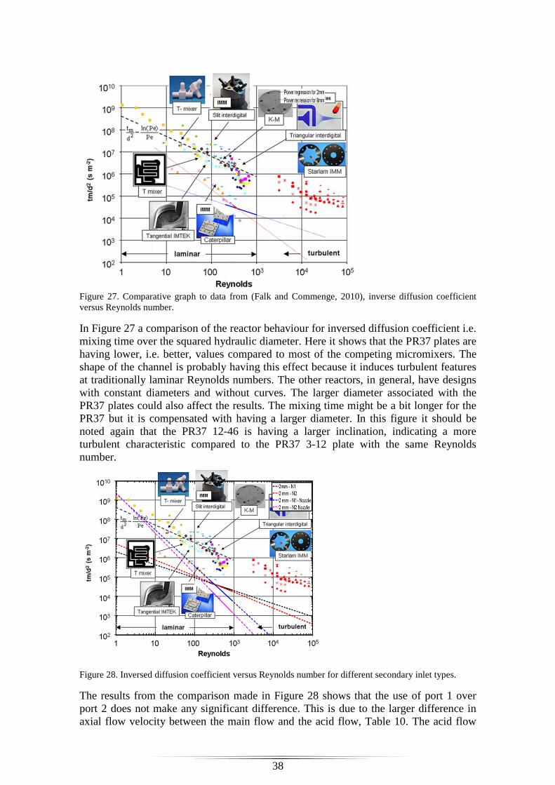
38

Figure 27. Comparative graph to data from (Falk and Commenge, 2010), inverse diffusion coefficient versus Reynolds number.

In Figure 27 a comparison of the reactor behaviour for inversed diffusion coefficient i.e. mixing time over the squared hydraulic diameter. Here it shows that the PR37 plates are having lower, i.e. better, values compared to most of the competing micromixers. The shape of the channel is probably having this effect because it induces turbulent features at traditionally laminar Reynolds numbers. The other reactors, in general, have designs with constant diameters and without curves. The larger diameter associated with the PR37 plates could also affect the results. The mixing time might be a bit longer for the PR37 but it is compensated with having a larger diameter. In this figure it should be noted again that the PR37 12-46 is having a larger inclination, indicating a more turbulent characteristic compared to the PR37 3-12 plate with the same Reynolds number.

Figure 28. Inversed diffusion coefficient versus Reynolds number for different secondary inlet types.

The results from the comparison made in Figure 28 shows that the use of port 1 over port 2 does not make any significant difference. This is due to the larger difference in axial flow velocity between the main flow and the acid flow, Table 10. The acid flow

39

rate is not large enough, without the use of nozzle at least, to reach the opposite wall at port 2 which is then resulting in not having T-mixer behaviour. The experiments using nozzle shows, although the results are not perfect, a trend quite similar to the behaviour of the PR37 12-46. The reason is probably due to the enhanced dispersion at the inlet which is spreading the fluid more effectively compared to not using a nozzle, the acid-base neutralisation, ( i ), is then occurring more effectively because of the increased initial mixing.

A new adaptive procedure for using chemical probes to characterize mixing The second study is a study performed at the University of Nantes, France, (Falk and Commenge, 2010) in this study they use the same adaptive procedure as in the current project aiming for a constant reaction volume for all experiments. The design of the reactor is also similar to the design of the ART Plate Reactors but in their study they use a nozzle of 500 µm, a reactor with a characteristic diameter similar to the PR 37 6-23 the main difference in the study at Nantes compared to the current one is that they study mixing at higher Reynolds numbers. In the study the final mixing times are not revealed a rough estimation can be made from the reported segregation index and their illustration of the segregation versus mixing time graph. The results from the Nantes study are in the same region as the results from the current study.

Comparison with batch reactors Studies using the Villermaux-Dushman protocol for studying the mixing in batch reactors have been performed by a number of scientists, the method was originally developed for characterizing batch reactors. In the current project results from the studies performed by (Fournier et al., 1996a) and (Assirelli et al., 2008) have been used for comparison. The Assirelli study is performed in a batch reactor with a diameter of 0.29 m and liquid height of 0,38 m and is operating at very high Reynolds numbers. In the study both micromixing time and macromixing time, what is generally called mixing time, are measured. For the micromixing time the results, Table 13, and Figure 29, indicates that the batch reactor has a better ratio between dissipation rate and mixing time compared to the ART® Plate Reactors investigated. But in the batch reactor the micromixing times vary throughout the reactor being smallest close to the impeller and larger at the surface. This means that the micromixing time is very dependent upon where in the reactor you are, this is due to the lowered energy dissipation due to the distance to the impeller. In the Assirelli study the micromixing time results differ 3000% from the fastest to the slowest. The Fournier study shows similar results, unfortunately the raw data is not available from that study. Although this phenomena has not been studied in the ART® Plate Reactors a difference in mixing along the reactor is not expected since the design of the channel is repetitive. For chemical reactions the yield and concentration of the end product are the vital parameters, hence the uniformity of the reactor liquid is important. The macromixing studies performed by Assirelli indicate that the uniformity of the species concentration quite bad. The results indicate that the macromixing time is in the region of tens of

40

seconds. For the ART® Plate Reactor the method used accounts for all types of mixing, although micromixing is the most prominent. When using the batch reactor compared to the ART® Plate Reactors the mixing time might be lower, depending on where your inlet is situated. The operation of batch reactors compared to continuous is associated with concentration gradients due to varying mixing efficiency, this results in the use of a larger ratio between the bulk volume and reactant volume resulting in lower end product concentration. In the continuous operation the mixing is uniform and well controlled which enables significant process intensification, producing highly concentrated end products with a high conversion rate. Table 13. The micromixing results from the Assirelli study

Position 1U 1 3U 3Ua 3 4U 4Ua 4Ub 4Uc 4

tm [s] 0,0135 0,105 0,0063 0,004 0,017 0,0035 0,0045 0,004 0,0069 0,0035

εT [W/kg] 1,66 0,03 7,62 18,1 1 23,6 14,8 18,6 6,97 24,3

In the table U means unbaffled and a, b, c means at the same axial position but on varying distance from the impeller.

Figure 29. Comparison with Assirelli on the base of Reynolds number

High-Throughput Microporous Tube-in-Tube Microchannel Reactor A study performed at Beijing University of Chemical Technology (Wang et al., 2009) has investigated micromixing in a tube-in-tube reactor they call MTMCR. The results from this study though are hard to interpret, the study has not compiled a table of the final results. They have also not supplied a segregation index versus mixing time for the range of acid they have used. This means that the reader cannot estimate the resulting mixing time. This would have been a good reactor to compare with since it has a very wide range of flow rates which goes beyond the maximum limit for the PR37. When the segregation index versus mixing time curve has been derived using their stated inlet concentrations and flow rates the mixing time seems to be very high. The results are in the region of several hundred of milliseconds for the same flow rates used in the current project (100 ml/min). One of the assumptions made in the current project is confirmed in the Wang study. This is that the mixing time versus flow rate curve is flattening after a certain flow, indicating that the flow is fully turbulent and for the increasing flow rate no enhancement in mixing performance is observed.

41

Pre-study In the pre-study, performed by Alfa Laval and University of Eindhoven, they have used the minimum length between walls as hydraulic diameter and they have also studied much higher flows than in the current project. The concentrations used in the study yields a much shorter reaction time, one third of the what the current project uses, for the second reaction indicating that it is more the initial inlet mixing which is characterised rather than the channel design. The pre-study also uses the same concentration and reaction time for all the experiments. For the comparable experiments the mixing times are in the same region as the results from this study. The half nominal flows the mixing times are not very comparable, but for the other three measurements with similar flow the results correspond well and are well within the ±30% limit. This indicates that the method is replicable, although the pre-study have used a different approach to the Villermaux/Dushman system.

42

Conclusions As have been discussed in the previous two paragraphs the results from the project are corresponding well to previous studies. The method used to characterise the mixing is a global method, it includes all types of mixing present macro-, meso- and micromixing. However the mixing most prominent in the ART Plate Reactor PR37-series is the micromixing, because the channels are narrow and Reynolds numbers are low, The Villermaux/Dushman method is also aiming to characterise this with the use of chemical reactions. Compared to micromixers the ART Plate reactor series have a better efficiency in reduced mixing time when Reynolds number is increased, i.e. flow rate is increased, compared to the micromixers. This is probably associated with the design of the ART Plate Reactors, inducing vortices and Dean vortices in Reynolds regions traditionally associated with laminar conditions. The results have shown that this effect is increased, or at least occurs at lower Reynolds numbers, when having a larger plate. For the PR37 3-12 the results are close to the theoretical value for laminar flow but for the PR37 12-46 plate the results corresponds very well to the theoretical values for turbulent flow. Comparisons to bath reactors are more difficult to perform since the design and measuring techniques are very different. Some conclusions can be made though, the ART® Plate Reactor has a more uniform mixing performance throughout the reactor, the mixing time is much higher in batch reactors and batch reactors generally produce low concentrated end products compared to a continuous solution. This paragraph has been classified.

Recommendations This section has been classified.

43

Future investigations The method has been confirmed to work for the characterisation of mixing time for the ART® Plate Reactors. In the future it would be interesting to investigate mixing at higher flow rates for all plate types, in order to achieve this a reliable pump for the acid flow rate is needed which also can handle back pressure well. The concentrations used in the current project are suitable for the flow rates in the present study. Since the absorbance measurements are on the maximum limit in some of the measurements a revision of the concentrations should be performed when testing larger flow rates. A study with higher resolution investigating the Dean vortex effect and wall effects for the different plates would also be interesting. This could yield an understanding to the indicated better mixing with the smallest plate. Such an investigation would need other experimental techniques though.

44

Bibliography ALFALAVAL 2005a. Alfa Laval ART® LabPlate™. CC00190EN 1011 ed. http://www.alfalaval.com/campaigns/labplatereactor/Downloads/Documents/CC00190EN.pdf. ALFALAVAL 2005b. Alfa Laval ART® Plate Reactor 37. CC00150EN 1108 ed. http://www.alfalaval.com/campaigns/stepintoart/downloads-

links/Documents/CC00150EN_ART%20PR%2037%20leaflet.pdf. ALFALAVAL 2005c. Alfa Laval ART® Plate Reactor 49. CC00182EN 0910 ed. http://www.alfalaval.com/campaigns/stepintoart/downloads-links/Documents/CC00182EN.pdf. ASSIRELLI, M., BUJALSKI, W., EAGLESHAM, A. & NIENOW, A. W. 2008. Macro- and

micromixing studies in an unbaffled vessel agitated by a Rushton turbine. Chemical Engineering Science, 63, 35-46.

AUBIN, J., FERRANDO, M. & JIRICNY, V. 2010. Current methods for characterising mixing and flow in microchannels. Chemical Engineering Science, 65, 2065-2093.

BALDYGA, J. & BOURNE, J. R. 1989. Simplification of micromixing calculations .1. Derivation and application of new model. Chemical Engineering Journal and the Biochemical Engineering Journal, 42, 83-92.

BALDYGA, J. & BOURNE, J. R. 1990. Comparison Of The Engulfment And The Interaction-By-Exchange-With-The-Mean Micromixing Models Chemical Engineering Journal and the Biochemical Engineering Journal, 45, 25-31.

BALDYGA, J. & BOURNE, J. R. 1994. Principles of Micromixing. In: CHEREMISINOFF, N. P. (ed.) Encyclopedia of fluid mechanics. Houston, Texas: Gulf Publishing Co.

BAŁDYGA, J. & BOURNE, J. R. 1999. Turbulent mixing and chemical reactions, Wiley. BAŁDYGA, J. & POHORECKI, R. 1995. Turbulent micromixing in chemical reactors — a review. The

Chemical Engineering Journal and the Biochemical Engineering Journal, 58, 183-195. BOUAIFI, M., MORTENSEN, M., ANDERSSON, R., ORCIUCH, W., ANDERSSON, B., CHOPARD,

F. & NOREN, T. 2004. Experimental and numerical investigations of a jet mixing in a multifunctional channel reactor - Passive and reactive systems. Chemical Engineering Research & Design, 82, 274-283.

BOURNE, J. R. 1997. Chapter 10 - Mixing in single-phase chemical reactors. In: HARNBY, N., EDWARDS, M. F. & NIENOW, A. W. (eds.) Mixing in the Process Industries. Oxford: Butterworth-Heinemann.

BOURNE, J. R. 2008. Comments on the iodide/iodate method for characterising micromixing. Chemical Engineering Journal, 140, 638-641.

BOURNE, J. R., KOZICKI, F. & RYS, P. 1981. Mixing and fast chemical-reaction .1. Test reactions to determine segregation. Chemical Engineering Science, 36, 1643-1648.

COMMENGE, J.-M. & FALK, L. 2011. Villermaux-Dushman protocol for experimental characterization of micromixers. Chemical Engineering and Processing, 50, 979-990.

COSTA, P. & TREVISSOI, C. 1972. Reactions with non-linear kinetics in partially segregated fluids. Chemical Engineering Science, 27, 2041-2054.

EDWARDS, M. F. 1997. Chapter 11 - Laminar flow and distributive mixing. In: HARNBY, N., EDWARDS, M. F., A.W. NIENOWA2 - N HARNBY, M. F. E. & NIENOW, A. W. (eds.) Mixing in the Process Industries. Oxford: Butterworth-Heinemann.

EHRFELD, W., GOLBIG, K., HESSEL, V., LOWE, H. & RICHTER, T. 1999. Characterization of mixing in micromixers by a test reaction: Single mixing units and mixer arrays. Industrial & Engineering Chemistry Research, 38, 1075-1082.

FALK, L. & COMMENGE, J. M. 2010. Performance comparison of micromixers. Chemical Engineering Science, 65, 405-411.

FOURNIER, M. C., FALK, L. & VILLERMAUX, J. 1996a. A new parallel competing reaction system for assessing micromixing efficiency - Determination of micromixing time by a simple mixing model. Chemical Engineering Science, 51, 5187-5192.

FOURNIER, M. C., FALK, L. & VILLERMAUX, J. 1996b. A new parallel competing reaction system for assessing micromixing efficiency - Experimental approach. Chemical Engineering Science, 51, 5053-5064.

GUICHARDON, P., FALK, L. & ANDRIEU, M. 2001. Experimental comparison of the iodide-iodate and the diazo coupling micromixing test reactions in stirred reactors. Chemical Engineering Research & Design, 79, 906-914.

GUICHARDON, P., FALK, L. & VILLERMAUX, J. 2000. Characterisation of micromixing efficiency by the iodide-iodate reaction system. Part II: kinetic study. Chemical Engineering Science, 55, 4245-4253.

45

HABCHI, C., DELLA VALLE, D., LEMENAND, T., ANXIONNAZ, Z., TOCHON, P., CABASSUD, M., GOURDON, C. & PEERHOSSAINI, H. 2011. A new adaptive procedure for using chemical probes to characterize mixing. Chemical Engineering Science, 66, 3540-3550.

HARADA, M., ARIMA, K., EGUCHI, W. & NAGATA, S. 1962. Micro-Mixing in a Continous Flow Reactor (Coalescence and Redispersion Models). The Memoirs of the Faculty of Engineering. Kyoto University.

HENDERSHOT, D. C. & SARAFINAS, A. 2005. Safe chemical reaction scale up. Chemical Health and Safety, 12, 29-35.

HESSEL, V. 2009. Micro process engineering : a comprehensive handbook, Weinheim, Wiley-VCH. JOHNSON, B. K. & PRUD'HOMME, R. K. 2003. Chemical processing and micromixing in confined

impinging jets. Aiche Journal, 49, 2264-2282. KASHID, M., RENKEN, A. & KIWI-MINSKER, L. 2011. Mixing efficiency and energy consumption

for five generic microchannel designs. Chemical Engineering Journal, 167, 436-443. KOCKMANN, N. 2008. Diffusion, Mixing, and Mass Transfer Equipment Transport Phenomena in Micro Process Engineering. Springer Berlin Heidelberg. MALECHA, K., GOLONKA, L. J., BALDYGA, J., JASINSKA, M. & SOBIESZUK, P. 2009.

Serpentine microfluidic mixer made in LTCC. Sensors and Actuators B-Chemical, 143, 400-413. PALMER, D. A., RAMETTE, R. W. & MESMER, R. E. 1984. Triiodide ion formation equilibrium and

activity coefficients in aqueous solution. Journal of Solution Chemistry, 13, 673-683. RUASSE, M. F., AUBARD, J., GALLAND, B. & ADENIER, A. 1986. Kinetic study of the fast halogen-

trihalide ion equilibria in protic media by the Raman-laser temperature-jump technique. A non-diffusion-controlled ion-molecule reaction. Journal of Physical Chemistry, 90, 4382-4388.

WANG, Q.-A., WANG, J.-X., YU, W., SHAO, L., CHEN, G.-Z. & CHEN, J.-F. 2009. Investigation of Micromixing Efficiency in a Novel High-Throughput Microporous Tube-in-Tube Microchannel Reactor. Industrial & Engineering Chemistry Research, 48, 5004-5009.

VILLERMAUX, J. 1996. Trajectory Length Distribution (TLD), a novel concept to characterize mixing in flow systems. Chemical Engineering Science, 51, 1939-1946.

VILLERMAUX, J. & DEVILLON, J. Représentation de la coalescence et de la redispersion des domaines de ségrégation dans un fluide par un modèle d’interaction phénoménologique. The fifth European/ second International Symposium on Chemical Reaction Engineering, 2, 3 and 4 May 1972 Amsterdam, the Netherlands. Elsevier Pub. Co., B1-B13.

VILLERMAUX, J. & FALK, L. 1994. A generalized mixing model for initial contacting of reactive fluids. Chemical Engineering Science, 49, 5127-5140.

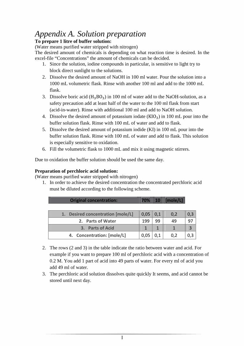
I

Appendix A. Solution preparation To prepare 1 litre of buffer solution: (Water means purified water stripped with nitrogen) The desired amount of chemicals is depending on what reaction time is desired. In the excel-file “Concentrations” the amount of chemicals can be decided.

1. Since the solution, iodine compounds in particular, is sensitive to light try to block direct sunlight to the solutions.

2. Dissolve the desired amount of NaOH in 100 ml water. Pour the solution into a 1000 mL volumetric flask. Rinse with another 100 ml and add to the 1000 mL flask.

3. Dissolve boric acid (H BO ) in 100 ml of water add to the NaOH-solution, as a safety precaution add at least half of the water to the 100 ml flask from start (acid-in-water). Rinse with additional 100 ml and add to NaOH solution.

4. Dissolve the desired amount of potassium iodate (KIO ) in 100 mL pour into the buffer solution flask. Rinse with 100 mL of water and add to flask.

5. Dissolve the desired amount of potassium iodide (KI) in 100 mL pour into the buffer solution flask. Rinse with 100 mL of water and add to flask. This solution is especially sensitive to oxidation.

6. Fill the volumetric flask to 1000 mL and mix it using magnetic stirrers.

Due to oxidation the buffer solution should be used the same day. Preparation of perchloric acid solution: (Water means purified water stripped with nitrogen)

1. In order to achieve the desired concentration the concentrated perchloric acid must be diluted according to the following scheme.

Original concentration: 70% 10 [mole/L]

1. Desired concentration [mole/L] 0,05 0,1 0,2 0,3

2. Parts of Water 199 99 49 97

3. Parts of Acid 1 1 1 3

4. Concentration: [mole/L] 0,05 0,1 0,2 0,3

2. The rows (2 and 3) in the table indicate the ratio between water and acid. For

example if you want to prepare 100 ml of perchloric acid with a concentration of 0.2 M. You add 1 part of acid into 49 parts of water. For every ml of acid you add 49 ml of water.

3. The perchloric acid solution dissolves quite quickly It seems, and acid cannot be stored until next day.

II

Appendix B. Procedure for calibration To produce a calibration curve of triiodide for spectrometer: (Water means purified water stripped with nitrogen) The basis for the calibration is to mix solutions of potassium iodide (KI) and iodine. These will react according to the equilibrium reaction:

�� + � ⇌ � � The equilibrium is very temperature dependent, all solutions should be of the same known temperature. The simplest way is to have them at room temperature. From previous measurement the Lambert-Beer law is expected to be valid for concentration lower than 5 ∗ 10�@ mole/L. The solutions prepared should be around this concentration. Iodine has a poor solubility in water with a maximum of about 1,14 ∗ 10� mole/L. This should be remembered when preparing the solutions. Using the constructed MatLab-file “calibration_concentration.m” it is possible to calculate the concentration of � � from a set of mixing ratios between the solutions. Example: The concentrations I use are 3 ∗ 10� for potassium iodide and 8 ∗ 10�Sfor iodine. In the table below you see the different volume mixed and also the concentration of triiodide this yields at a temperature of 293 K.

Vol KI-solution [ml] Vol I2-solution [ml] Vol water [ml] [I3-] mol/L 2 25 73 7,90E-06 5 25 70 1,88E-05 10 25 65 3,46E-05 15 25 60 4,81E-05 2 50 48 1,40E-05 5 50 45 3,36E-05 10 50 40 6,30E-05 15 50 35 8,87E-05 2 75 23 1,89E-05 5 75 20 4,56E-05 10 75 15 8,65E-05 15 75 10 1,23E-04

The solutions are prepared using dilution for the potassium iodide by making the concentration 20 times stronger than needed and then take 5% of that solution and dilute it by a factor 20 again, this due to the limitations of the available scales. For the iodine, which is less solvable in water, another technique is used. This time the total volume of the solution produced is increased by a factor instead. This produces more waste but a lot higher accuracy on the measurements. OBS! Iodine takes LONG time to dissolve in water. Recommended to start in afternoon and run over night. Because of the lack of 100 mL volumetric flasks the 50 mL volumetric flasks will be used instead. This is done by dividing the above table with two. The concentrations will be the same. Also due to insufficient stirring equipment the 12 volumetric flasks of 50 ml will be manually shaken every 15 minutes for 3 hours. This is to ensure that the equilibrium has been achieved in the flask. Calibration_concentration.m This MatLab-file computes the expected concentration of triiodide for the different mixtures in your experiment. It is the first six rows of data which should be changed to the settings you have used. The data needed is: temperature [K], base solution concentration of KI and I2, the volume of KI and I2 added to the respective flask and the desired total volume.

III

Appendix C. Spectrometer instructions Instructions for operating the Spectrometer, in order to measure absorbance The computer which the spectrometer is to be connected to must have the AvaSoft software installed. It is downloadable from Avantes homepage or you could install it from the CD. The homepage will supply the newest version of the software. The spectrometer is telling the software what version it should be running (FULL). Basic start-up instructions

1. Connect DC 12V source to AvaLight DHc. 2. Connect USB cable between AvaSpec and PC. 3. Connect the optical fibre cables from light source to flow cell and from flow cell

to spectrometer. 4. Start the light source. Choose correct lamps (DH for both deuterium and

halogen). It takes about 10 minutes for the lamp to start up. 5. Set the light source ”ON” on the OFF-TTL-ON switch. 6. Start the AvaSoft software on the computer. 7. Start a new experiment: File->”Start New Experiment”, if you’re not doing this

you are on the same experiment file which was used last time.

The integration time has to be set correctly. It is important that this setting is the same for all experiments, since it affects the value of the measured absorbance. The integration time should be the same both during experiments and for the calibration curve. Settings for absorbance measurement

- There is a button in AvaSoft called ”Autoconfigure integrationtime”. This automatically sets the integration time to a value where the maximum ”Counts” are 85% of the maximum value (65 000 for 64-bit system). This function might be useful, but it is focusing on the entire wavelength range and not the specific one you might be interested in.

- The ”Average” setting sets the number of integration time the software should average over. The Autoconfigure sets this value in order for the spectra to update with a frequency of 2 Hz, “Integration time”*Average = 500 ms.

- The average-value does not affect the spectrum.

My recommendation would be to use the buffer solution and pump it through the flow cell. Then adjust the integration time to have a reasonable amount of counts (40 000-50 000) in the region of which you are interested. During the experiments in the Master Thesis the settings were; Integration time: 33 ms, Average: 15. You press “Start” to start the measurement and produce a Scope.

8. Save your experiment with a name and in a folder you can find later. File->Save->Experiment

9. Using the desired reference solution (recommended purified water of buffer solution, purified water used in the Master Thesis) a reference must be saved in order for the software to produce an absorbance spectra. With the desired solution flowing through the flow cell press the white square “Save reference” or File->Save->Reference.

IV

10. Save a dark reference by shifting the ”OFF-TTL-ON” switch to ”OFF”. Press the black square “Save Dark” of File->Save->Dark. Shift the witch back to “ON”.

Now the spectrometer software should be ready to measure absorbance spectra. You can test this by switching from Scope to Absorbance by pressing the blue A or view “Absorbance view”. With the solution used for reference this should show nothing. History channels (data logging) Now you are ready to measure the absorbance of the reactants. Before starting you should set up the “History channels”. In Application->History->Function entry you can set up to 8 different measurements which you want recorded for your experiments. Setting the radio buttons to “User defined”, “Absorbance”, “Input function” and writing m(XXX) as function will display the absorbance at XXX nm. You can also save e.g. entire spectrums.

You can either save your data to a .dat file under the Function entry settings of if you want the data from your history channels to be saved to an Excel file you can set this under Application->Excel Output (if the AvaSoft-XLS add-on is bought). When you are using the Excel output, remember to Enable it under Application->Excel Output

V

Appendix D. Calculations in Excel This appendix has been classified.

VI

Appendix E. Concentration excel-file This appendix has been classified.

VII

Appendix F. Absorbance graphs

Figure 30. PR37 0.8-2.2, 0.5*Nominal, Port 1

Figure 31. PR37 0.8-2.2, 1*Nominal, Port 1

VIII

Figure 32. PR37 3-12, 0.5*Nominal, Port 1

Figure 33. PR37 3-12, 0.5*Nominal, Port 2

Figure 34. PR37 3-12, 1*Nominal, Port 1

IX


Figure 36. PR37 3-12, 2*Nominal, Port 1.


X

Figure 38. PR37 12-46, 0.5*Nominal, Port 1.

Figure 39. PR37 12-46, 1*Nominal, Port 1.

Figure 40. PR37 3-12, 0.5*Nominal, Port 1 and 2, Nozzle

XI

Figure 41. PR37 3-12, 1*Nominal, Port 1 and 2, Nozzle

Figure 42. PR37 3-12, 2*Nominal, Port 1 and 2, Nozzle

XII

Appendix G. MatLAB-script for mixing time graph function xstotmcalc(dataq10, dataq20, datacH0, dataXS) %% % This function file calculates the graph of X_S ve rsus t_m for the given % input of buffer flow rate, acid flow rate, concen tration of acid and the segregation index. data.q10 =dataq10; % Just translating the in varibles into the variabl es used in the script. data.q20 =dataq20; % This is what happens when you build the code firs t and realize you need input later. data.cH0 =datacH0; % Aslo MatLab for some reason doesn't accept the da ta.XXX as input variables. % Concentration of buffert used during experiments . Since this is constant % for all the experiments it is not an input variab le. data.cH2BO30=XXX; % mol/l data.cH3BO30=XXX; % mol/l data.cIO30=XXX; % mol/l data.cI0=XXX; % mol/l data.q10/data.q20; % Calculating flow ratio buffer/acid data.qout=data.q10+data.q20; % Total flow rate % Acid concentration is varying and graph must be c alculated for all data.cH0_matrix = data.cH0; % mol/l figure; for k = 1:length(data.cH0_matrix); data.cH0 = data.cH0_matrix(k); % Rate constants for the reactions, data.k3=5.6e9; % l/mol/s Data from Ruasse data.k3r=7.5e6; % /s Data from Ruasse data.pka=9.14; % first reaction %% % 1=H+ 2=I- 3=IO3- 4=I2 5=I3- 6=H2BO3- 7=H3BO3 % Con--acid phase % Con_mix--bulk mixture at the outlet global k2 NN=21; % Number of points in tm XS=zeros(1,NN); % Segregations index starts @ 0 tm=logspace(-3,2,NN); % tm dividide in NN-1 equal intervalls from 10^-3 t o 10^2 for i=1:length(tm) % for every setpoint of tm. data.tm=tm(i); % Set data.tm to be the specifed set point Con0=[data.cH0;0;0;0;0;0;0;]; % Start concentration of acid solution % options=odeset('Events',@events,'RelTol',1e-1 4,'AbsTol',1e-14); % t_max=1e5; options=odeset( 'RelTol' ,3e-14, 'AbsTol' ,1e-14); % Setting tolerances for ode-solver t_max=data.tm*log(data.qout/data.q20); [t,Con]=ode15s(@odefun,[0 t_max],Con0,options,d ata); % Solves the equation system Con0 Da2(i)=tm(i)*k2*data.cH0^4; XS(i)=2*(data.qout*(Con(end,4)+Con(end,5))/(data.q2 0*data.cH0))*(1+data.cH2BO30/(6*data.cIO30)); % yields a XS corresponding to each specified tm end colors = colormap(hsv(4)); %cftool(tm, XS) % Starts curve fitting tool when wanted loglog(tm,XS, 'Color' , colors(k, :), 'DisplayName' , sprintf( '[H^+] = data.cH0_matrix(%d)' , k)) hold on if length(dataXS)>1.5

XIII

for h=1:length(dataXS) plot([10^-3, 10^2], [dataXS(h), dataXS(h)]) end else plot([10^-3, 10^2], [dataXS, dataXS]) end xlabel( 't_m' ) ylabel( 'X_S' ) legend(num2str(data.cH0_matrix)) end return function dCon= odefun(t,Con,data) %% This is the function describing the equation sys tem which is to be solved. Con(8:14)=[0;data.cI0;data.cIO30;0;0;data.cH2BO30;d ata.cH3BO30;]; mu=1/2*(Con(1)+data.cH2BO30+data.cH0*0.5*2^2+(data. cIO30+data.cI0)+Con(2)+Con(3)+Con(5)+Con(6)); % Calculating the ionic strength % 1=H+ 2=I- 3=IO3- 4=I2 5=I3- 6=H2BO3- 7=H3BO3 global k2 if mu>0.166 k2=10^(8.383-1.511* sqrt(mu)+0.237*mu); else k2=10^(9.281-3.664*sqrt(mu)); end % Produced - Consumed + (Conc_buffer- conc_syra)/t_ m % No literature value has been found on the instant aneous reaction rate, it has been set to a 1000 times larger than the second reaction. Te sts showed that it wasn’t so important as long as it was >> than r2. dCon=zeros(7,1); % a column vector dCon(1)=-k2*1000*(Con(1)*Con(6)-10^(-data.pka)*Con( 7))-6*k2*Con(1)^2*Con(2)^2*Con(3)+(Con(8)-Con(1))/data. tm; dCon(2)=-5*k2*Con(1)^2*Con(2)^2*Con(3)-(data.k3*Con (2)*Con(4)-data.k3r*Con(5))+(Con(9)-Con(2))/data.tm; dCon(3)=-k2*Con(1)^2*Con(2)^2*Con(3)+(Con(10)-Con(3 ))/data.tm; dCon(4)=3*k2*Con(1)^2*Con(2)^2*Con(3)-(data.k3*Con( 2)*Con(4)-data.k3r*Con(5))+(Con(11)-Con(4))/data.tm; dCon(5)=data.k3*Con(2)*Con(4)-data.k3r*Con(5)+(Con( 12)-Con(5))/data.tm; dCon(6)=-k2*1000*(Con(1)*Con(6)-10^(-data.pka)*Con( 7))+(Con(13)-Con(6))/data.tm; dCon(7)=k2*1000*(Con(1)*Con(6)-10^(-data.pka)*Con(7 ))+(Con(14)-Con(7))/data.tm; return