investigations into microgrid sizing and energy …
TRANSCRIPT

INVESTIGATIONS INTO MICROGRIDSIZING AND ENERGY MANAGEMENT STRATEGIES
Yara Jamil Khawaja
A Thesis Submitted for the Degree of
Doctor of Philosophy at Newcastle University
School of Engineering
Faculty of Science, Agriculture and Engineering
August 2019

Yara Jamil Khawaja: Investigation into Microgrid Sizing and Energy Management
Strategies ©2019

D E C L A R AT I O N
I hereby declare that this thesis is my own work and effort and that it has not
been submitted anywhere for any award. Where other sources of information
have been used, they have been acknowledged.
Newcastle upon Tyne, 2019
Yara Jamil Khawaja

C E R T I F I CAT E O F A P P R OVA L
We confirm that, to the best of our knowledge, this thesis is from the student’s
own work and effort, and all other sources of information used have been ac-
knowledged. This thesis has been submitted with my approval.
Dr. Damian Giaouris
Dr. Adib Allahham
Dr. Charalampos Patsios
Dr. Mohamed Dahidah

To Issa, Hani, Morad, and Bassel
— Yara

A C K N O W L E D G E M E N T S
I would like to express my deep gratitude to my supervisors Dr. Damian Giaouris,
Dr. Adib Allahham, Dr. Charalampos Patsios, and Dr. Mohamed Dahidah for
their wisdom and guidance through my PhD journey. They have always been a
source of motivation and my inspirational model as a researcher.
I am grateful to the Applied Science Private University in Jordan for funding
my PhD study and for their support.
I would like also to express my gratefulness and appreciation to my colleagues
and friends in the School of Engineering, especially those in Power System
Research Group.
Thank you, my father, my mother and my mother-in-law, without your un-
conditional support, this thesis never would have come to be. Finally, and most
importantly, I am thankful to my lovely family, Issa my wonderful husband and
my lovely sons Hani, Morad and Bassel for all of their love, support, motivation
and patience throughout my PhD. They were there to help me at difficult times,
and to share in good times. Their encouragement has helped me with the research
and with the writing of this thesis, and I am very grateful.
vi

A B S T R A C T
The evolution of microgrids represents a significant step towards the transition to
more sustainable power systems. Recent trends in microgrids include the integra-
tion of renewable energy resources (RERs), alternative energy resources (AERs)
and energy storage systems (ESSs). However, the integration of these systems
creates new challenges on microgrid operation because of their stochastic and
intermittent nature. To mitigate these challenges, determining the appropriate
size together with the best energy management strategy (EMS) systems are
essential to ensure economic and optimal performance.
This thesis presents an investigation into sizing and energy management of
microgrids. In the first part of the thesis, an analytical and economic sizing (AES)
approach is developed to find the optimal size of a grid-connected photovoltaic-
battery energy storage system (PV-BESS). The proposed approach determines
the optimal size based on the minimum levelised cost of energy (LCOE). Funda-
mental to this approach obtains an improved formula of LCOE which includes
new parameters for reflecting the impact of surplus PV energy and the energy
purchased from the grid.
In the second part of this thesis, an integrated framework is proposed for
finding the best size-EMS combination of a stand-alone hybrid energy system
(HES). The HES consists of PV, BESS, diesel generator, fuel cell, electrolyser, and
hydrogen tank. The proposed framework includes three consecutive steps; first,
performing the AES to obtain the initial size of the HES, second, implementing
the initial EMS using finite automata (FA) and instantiating multiple EMSs;
and third, developing an evaluation model to assess the instantiated EMSs and
extract the featured conditions to produce an improved EMS. Then the AES
approach is re-exercised using the improved EMS to obtain the best size-EMS
combination. The core of this framework is utilising FA to implement various
EMSs and capturing the impact of selecting the best EMS on the sizing of the
HES.
Furthermore, a sensitivity analysis is performed to address the uncertainty in
demand and solar radiation data showing their effect on the HES performance.
The analysis is carried out by assuming variations in solar radiation and demand
annual data. Several scenarios are generated from the sensitivity analysis, and a
number of performance indices are computed for each scenario. Following that, a
vii

fuzzy logic controller is designed using the performance indices as fuzzy input
sets. The objective of this controller is to modify the EMS obtained from the
integrated framework. This can be accomplished by detecting any changes in the
demand and solar radiation and accordingly modify the operating conditions of
the diesel generator, fuel cell, and electrolyser.
The performance of the proposed approaches is validated using real datasets
for both demand and solar radiation. The results show the optimal size and EMS
for both grid-connected and stand-alone microgrids. Moreover, the designed fuzzy
logic controller enables the microgrid to mitigate the uncertainty in the demand
and generation data.
The proposed approaches can be used with various scales of microgrids to
extract manifold benefits where reliability, environmental and cost requirements
can not be tolerated.
viii

P U B L I CAT I O N S A N D C O N T R I B U T I O N S
The publications that were produced as a part of the research reported in this
thesis are listed as follows:
Journal publications:
• Yara Khawaja; Adib Alhham; Damian Giaouris; Charalmpos Patsios; Sara
Walker; Mohamed Dahadih; Issa Qiqieh; An Integrated Framework for Sizing
and Energy Management for Hybrid Energy System using Finite Automata,
Applied Energy, Elsevier, Volume 250, 2019, pp. 257-272.
• Yara Khawaja; Adib Alhham; Damian Giaouris; Charalmpos Patsios; Modi-
fying the Energy Management of a Hybrid Energy System using Fuzzy Logic
(to be submitted to Applied Energy, Elsevier).
Conference publications:
• Yara Khawaja; Damian Giaouris; Charalmpos Patsios; Mohamed Dahadih;
Optimal cost-based model for sizing grid-connected PV and battery energy
system, 2017 IEEE Jordan Conference on Applied Electrical Engineering and
Computing Technologies (AEECT), Amman, 2017, pp. 1-6.
• Yara Khawaja; Adib Allahham, Damian Giaouris; Charalampos Patsios; and
Mohamed Dahidah; Supervision Control and Energy Management Strategies
for Grid-Connected Microgrids Using Finite Automata, UKES 2018.
ix

C O N T E N T S
I Thesis Chapters 1
1 I N T R O D U C T I O N 2
1.1 Motivation . . . . . . . . . . . . . . . . . . . . . . . . . . . . . . . . . 2
1.1.1 Sizing of Microgrids . . . . . . . . . . . . . . . . . . . . . . . 3
1.1.2 Energy Management Strategies . . . . . . . . . . . . . . . . 5
1.2 Thesis Scope and Contributions . . . . . . . . . . . . . . . . . . . . . 6
1.3 Thesis Overview . . . . . . . . . . . . . . . . . . . . . . . . . . . . . . 8
2 BA C K G R O U N D A N D L I T E R AT U R E S U R V E Y 10
2.1 Introduction . . . . . . . . . . . . . . . . . . . . . . . . . . . . . . . . 10
2.2 Microgrids . . . . . . . . . . . . . . . . . . . . . . . . . . . . . . . . . . 10
2.2.1 Microgrid Benefits and Drawbacks . . . . . . . . . . . . . . 11
2.2.2 Microgrids Modes . . . . . . . . . . . . . . . . . . . . . . . . . 13
2.3 Energy Storage Systems . . . . . . . . . . . . . . . . . . . . . . . . . 14
2.4 Hybrid Energy Systems . . . . . . . . . . . . . . . . . . . . . . . . . 16
2.5 Criteria for Microgrid Optimisation . . . . . . . . . . . . . . . . . . 17
2.5.1 Reliability Assessment . . . . . . . . . . . . . . . . . . . . . . 18
2.5.2 Economic Assessment . . . . . . . . . . . . . . . . . . . . . . 20
2.5.3 Environmental Assessment . . . . . . . . . . . . . . . . . . . 21
2.6 Control and Energy Management of Microgrids . . . . . . . . . . . 22
2.7 Finite Automata and Fuzzy Logic . . . . . . . . . . . . . . . . . . . . 25
2.7.1 Finite Automata and Discrete Event Systems . . . . . . . . 26
2.7.2 Fuzzy Logic . . . . . . . . . . . . . . . . . . . . . . . . . . . . 27
2.8 Microgrids Sizing Methods . . . . . . . . . . . . . . . . . . . . . . . . 28
2.8.1 Graphical Construction Methods . . . . . . . . . . . . . . . . 29
x

C O N T E N T S xi
2.8.2 Analytical Methods . . . . . . . . . . . . . . . . . . . . . . . . 30
2.8.3 Iterative Methods . . . . . . . . . . . . . . . . . . . . . . . . . 31
2.8.4 Probabilistic Methods . . . . . . . . . . . . . . . . . . . . . . 33
2.8.5 Artificial Intelligence Methods . . . . . . . . . . . . . . . . . 33
2.8.6 Hybrid Methods . . . . . . . . . . . . . . . . . . . . . . . . . . 35
2.8.7 Software Tools . . . . . . . . . . . . . . . . . . . . . . . . . . . 36
2.9 Concluding Remarks and Discussions . . . . . . . . . . . . . . . . . 39
3 S I Z I N G O F G R I D -C O N N E C T E D M I C R O G R I D 40
3.1 Introduction . . . . . . . . . . . . . . . . . . . . . . . . . . . . . . . . 40
3.2 Grid-connected PV-BESS Architecture . . . . . . . . . . . . . . . . . 41
3.3 Sizing Methodology of PV-BESS Grid-Connected . . . . . . . . . . 42
3.4 PV-BESS Analytical and Economic Model . . . . . . . . . . . . . . . 46
3.4.1 PV System Analytical Model . . . . . . . . . . . . . . . . . . 47
3.4.2 BESS Analytical Model . . . . . . . . . . . . . . . . . . . . . 49
3.4.3 The Economic Model of the Grid-connected PV-BESS . . . 50
3.5 Results and Discussion . . . . . . . . . . . . . . . . . . . . . . . . . . 54
3.6 Concluding Remarks . . . . . . . . . . . . . . . . . . . . . . . . . . . 64
4 T H E I N T E G R AT E D F R A M E W O R K 66
4.1 Introduction . . . . . . . . . . . . . . . . . . . . . . . . . . . . . . . . 66
4.2 HES Structure and Modelling in Finite Automata . . . . . . . . . . 68
4.2.1 HES Architecture . . . . . . . . . . . . . . . . . . . . . . . . . 68
4.2.2 Modelling the BESS in Finite Automata . . . . . . . . . . . 68
4.2.3 Implementing EMS using Finite Automata . . . . . . . . . 71
4.3 Analytical Modelling of HES . . . . . . . . . . . . . . . . . . . . . . . 77
4.3.1 Battery Energy Storage System . . . . . . . . . . . . . . . . 78
4.3.2 Diesel Generator . . . . . . . . . . . . . . . . . . . . . . . . . 83
4.3.3 Fuel Cell . . . . . . . . . . . . . . . . . . . . . . . . . . . . . . 84
4.3.4 Electrolyser . . . . . . . . . . . . . . . . . . . . . . . . . . . . 85
4.3.5 Hydrogen Tank . . . . . . . . . . . . . . . . . . . . . . . . . . 87
4.4 The Economic Modelling . . . . . . . . . . . . . . . . . . . . . . . . . 88

C O N T E N T S xii
4.4.1 Photovoltaic . . . . . . . . . . . . . . . . . . . . . . . . . . . . 89
4.4.2 Battery Energy Storage System . . . . . . . . . . . . . . . . 90
4.4.3 Diesel Generator . . . . . . . . . . . . . . . . . . . . . . . . . 90
4.4.4 Objective Function and Constraints . . . . . . . . . . . . . . 91
4.5 Initial Sizing . . . . . . . . . . . . . . . . . . . . . . . . . . . . . . . . 93
4.6 Integrated Framework . . . . . . . . . . . . . . . . . . . . . . . . . . 94
4.6.1 Instantiation of EMSs using Finite Automata . . . . . . . . 95
4.6.2 Performance Indices . . . . . . . . . . . . . . . . . . . . . . . 99
4.6.3 Evaluation Model and EMSinitial Replacement . . . . . . . 100
4.7 Results and Discussion . . . . . . . . . . . . . . . . . . . . . . . . . . 102
4.8 Concluding Remarks . . . . . . . . . . . . . . . . . . . . . . . . . . . 108
5 M O D I F Y I N G E N E R G Y M A N A G E M E N T U S I N G F U Z Z Y L O G I C 110
5.1 Introduction . . . . . . . . . . . . . . . . . . . . . . . . . . . . . . . . 110
5.2 Resizing the Hybrid Energy System using Forecasted Data . . . . 111
5.3 Sensitivity Analysis . . . . . . . . . . . . . . . . . . . . . . . . . . . . 113
5.4 Modify the EMS Using Fuzzy Logic . . . . . . . . . . . . . . . . . . 119
5.4.1 The design of Fuzzy Logic Controller . . . . . . . . . . . . . 119
5.4.2 The Fuzzy Rules . . . . . . . . . . . . . . . . . . . . . . . . . 124
5.4.3 The Results of Fuzzy Logic Controller . . . . . . . . . . . . 130
5.4.4 Validation Case Study . . . . . . . . . . . . . . . . . . . . . . 133
5.5 Concluding Remarks . . . . . . . . . . . . . . . . . . . . . . . . . . . 136
6 C O N C L U S I O N S A N D F U T U R E W O R K 137
6.1 Summary and Conclusions . . . . . . . . . . . . . . . . . . . . . . . . 137
6.2 Critical Review and Future Work . . . . . . . . . . . . . . . . . . . . 139
II Thesis Bibliography 141
B I B L I O G R A P H Y 142

L I S T O F F I G U R E S
Figure 1.1 The evolution of global total Photovoltaic (PV) installed
capacity from 2012 to 2020 [1]. . . . . . . . . . . . . . . . . . 4
Figure 2.1 Example of a microgrid including PV, Wind Turbine (WT),
Battery Energy Storage System (BESS), Diesel Genera-
tor (DSL) for a residential and industrial demand. The
presented microgrid can operate in both grid-connected and
stand-alone modes. . . . . . . . . . . . . . . . . . . . . . . . . 12
Figure 2.2 Types of Energy Storage Systems (ESSs) used in microgrids
and examples for each type. . . . . . . . . . . . . . . . . . . . 16
Figure 2.3 General architecture of Hybrid Energy System (HES) that
shows the diversity in the assets such as Renewable En-
ergy Resources (RERs), inverters, AC demand, DC demand,
ESSs and control unit representing the energy manage-
ment strategy. . . . . . . . . . . . . . . . . . . . . . . . . . . . 17
Figure 2.4 Evaluation criteria for sizing microgrids that classified into
reliability, economic and environmental assessment. . . . . 18
Figure 2.5 Energy Management System. . . . . . . . . . . . . . . . . . 23
Figure 2.6 Methods used for sizing microgrids with RERs and classi-
fied into seven methods. . . . . . . . . . . . . . . . . . . . . . 29
Figure 3.1 Grid-connected PV-BESS system consisting of PV, BESS,
inverter, and charge controller. . . . . . . . . . . . . . . . . . 41
Figure 3.2 The flowchart of the proposed Analytical and Economic
Sizing (AES) approach. . . . . . . . . . . . . . . . . . . . . . 44
Figure 3.3 Solar radiation of the Isle of Wight for one calendar year [2]. 45
Figure 3.4 Hourly ambient temperature profile for the Isle of Wight
for one calendar year [2] . . . . . . . . . . . . . . . . . . . . . 45
xiii

List of Figures xiv
Figure 3.5 Demand distribution of one calendar year [3]. . . . . . . . . 46
Figure 3.6 The relationship between different values PPV ,rated and
Levelised Cost of Energy (LCOE) for the three combina-
tions; PV-Lead-Acid Battery (LAB), PV-Lithuim Ion Bat-
tery (LIB), and PV-Redox Flow Battery (RFB). . . . . . . . 56
Figure 3.7 The relationship between different values PPV ,rated and
Levelised Cost of Delivery (LCOD) for the three BESSs;
LAB, LIB, and RFB. . . . . . . . . . . . . . . . . . . . . . . . 57
Figure 3.8 Energy purchased and extra PV energy sold to the grid
for the combination PV-LAB and PPV ,rated = 590 kW and
BatC = 1 MWh. . . . . . . . . . . . . . . . . . . . . . . . . . . 59
Figure 3.9 State of charge for lead-acid BESS for one calendar year. . 60
Figure 3.10 Energy purchased and extra PV energy sold to the grid-
for the combination PV-LIB and PPV ,rated = 710 kW and
BatC = 1 MWh. . . . . . . . . . . . . . . . . . . . . . . . . . . 61
Figure 3.11 State of charge for lithium-ion BESS for one calendar year. 62
Figure 3.12 Energy purchased and extra PV energy sold to the grid-
for the combination PV-LIB and PPV ,rated = 710 kW and
BatC = 1 MWh. . . . . . . . . . . . . . . . . . . . . . . . . . . 63
Figure 3.13 State of charge for redox flow BESS for one calendar year. 64
Figure 4.1 Stylized demonstration of three-step proposed framework:
(1) analytical and economic sizing; (2) using Finite Au-
tomata (FA) to generate various Energy Management
Strategy (EMS); and 3) evaluation model and feedback. . . 67
Figure 4.2 The network diagram of a stand-alone HES which consists
of PV, BESS, Fuel Cell (FC), Electrolyser (EL), Hydrogen
Tank (HT), DSL, and multiple inverters. . . . . . . . . . . . 69
Figure 4.3 Modelling BESS in finite automata. . . . . . . . . . . . . . . 70

List of Figures xv
Figure 4.4 Nine states describing EMSinitial based on finite au-
tomata. Each state illustrates which asset is operating and
whether the BESS and HT are charging or discharging.
The PV and demand are considered always as ON state . . 72
Figure 4.5 Finite automata model for EMSinitial . . . . . . . . . . . . . 72
Figure 4.6 The flowchart of AES approach showing the steps of the
EMS to find the initial size of the HES. . . . . . . . . . . . . 79
Figure 4.7 Hourly solar radiation profile for Newcastle upon Tyne city
for one calendar year [4]. . . . . . . . . . . . . . . . . . . . . 80
Figure 4.8 Hourly ambient temperature profile for Newcastle upon
Tyne city for one calendar year [4]. . . . . . . . . . . . . . . 81
Figure 4.9 Hourly demand profile for Newcastle upon Tyne citry for
one calendar year [5]. . . . . . . . . . . . . . . . . . . . . . . 82
Figure 4.10 Levelised cost of energy for the HES when using AES ap-
proach. . . . . . . . . . . . . . . . . . . . . . . . . . . . . . . . 93
Figure 4.11 Finite automata model for EMS1. . . . . . . . . . . . . . . . 96
Figure 4.12 Finite automata model for EMS2. . . . . . . . . . . . . . . . 97
Figure 4.13 Finite automata model for EMS3. . . . . . . . . . . . . . . . 99
Figure 4.14 Finite automata model for EMSnew. . . . . . . . . . . . . . 101
Figure 4.15 Levelised cost of energy for the HES when using integrated
framework. . . . . . . . . . . . . . . . . . . . . . . . . . . . . . 104
Figure 4.16 BESS soc, FC and PV power values during 48 hours in
June, the DSL output is zero during these hours. . . . . . . 105
Figure 4.17 BESS soc, FC, PV, DSL power and demand values during
48 hours in December. . . . . . . . . . . . . . . . . . . . . . . 106
Figure 4.18 HT socHT, EL,PV, and FC power values during 48 hours
in June. . . . . . . . . . . . . . . . . . . . . . . . . . . . . . . . 107
Figure 4.19 HT soc, EL,PV, and FC power values during 48 hours in
September. . . . . . . . . . . . . . . . . . . . . . . . . . . . . . 108

List of Figures xvi
Figure 5.1 An illustrative diagram showing the three stages required
to design a Fuzzy Logic Controller (FLC). Starting from
resizing the assets of the HES, conducting the sensitivity
analysis, then implementing the FLC to modify the original
EMS based on the output conditions set. . . . . . . . . . . . 111
Figure 5.2 Original and forecasted solar radiation of one calendar year.112
Figure 5.3 Original and forecasted demand distribution of one calen-
dar year. . . . . . . . . . . . . . . . . . . . . . . . . . . . . . . 112
Figure 5.4 The effect of demand and solar radiation variations on the
fuel cost. . . . . . . . . . . . . . . . . . . . . . . . . . . . . . . 117
Figure 5.5 The effect of demand and solar radiation variations on DSL
working hours. . . . . . . . . . . . . . . . . . . . . . . . . . . 117
Figure 5.6 The effect of demand and solar radiation variations on PV
contribution. . . . . . . . . . . . . . . . . . . . . . . . . . . . . 118
Figure 5.7 The configuration of the FLC introducing the input mem-
bership functions; fuel cost, WHDSL, and PV contribution.
The output membership function is the conditions sets that
modify the EMS. . . . . . . . . . . . . . . . . . . . . . . . . . 120
Figure 5.8 Membership function for fuel cost input fuzzy set. . . . . . 121
Figure 5.9 Membership function for WHDSL input fuzzy set. . . . . . . 121
Figure 5.10 Membership function for PV contribution input fuzzy set. 122
Figure 5.11 Membership function for output fuzzy sets. . . . . . . . . . 124
Figure 5.12 The fuel cost before and after applying the FLC. . . . . . . 132
Figure 5.13 The DSL working hours before and after applying the FLC. 132
Figure 5.14 The percentage of the PV contribution before and after
applying the FLC. . . . . . . . . . . . . . . . . . . . . . . . . . 133

L I S T O F TA B L E S
Table 2.1 Comparison of sizing methods available in the literature [6,
7, 8, 9]. . . . . . . . . . . . . . . . . . . . . . . . . . . . . . . . 38
Table 3.1 Cost and technical specifications of PV system used for
energy and cost calculations. . . . . . . . . . . . . . . . . . . 48
Table 3.2 Cost and technical specifications of the three types of BESS. 50
Table 3.3 Summary of the results obtained from Figure 3.6 regarding
the minimum LCOE at PPV ,rated = 710 kW and the value
of PV rated power at minimum LCOEsystem for the three
PV-BESS systems. . . . . . . . . . . . . . . . . . . . . . . . . 56
Table 3.4 LCOD for the three BESSs; LAB, LIB and RFB when
PPV ,rated = 710 kW. . . . . . . . . . . . . . . . . . . . . . . . . 56
Table 3.5 PV-LAB system, PV system only and Grid only scenarios,
where PPV ,rated=590 kW and LAB BatC=1 MWh . . . . . . 59
Table 3.6 PV-LIB system, PV system only and Grid only scenarios
where PPV ,rated=710 kW and LIB BatC=1 MWh . . . . . . 61
Table 3.7 PV-RFB system, PV system only and Grid only scenarios.
PPV ,rated=710 kW and RFB BatC=1 MWh . . . . . . . . . . 62
Table 3.8 PV-RFB components sizes. . . . . . . . . . . . . . . . . . . . 64
Table 4.1 Conditions for BESS operation. . . . . . . . . . . . . . . . . 70
Table 4.2 Conditions for EMSinitial . . . . . . . . . . . . . . . . . . . . 73
Table 4.3 Data used for PV analytical modele [10, 11]. . . . . . . . . . 80
Table 4.4 Data used for battery energy system modelling [10]. . . . . 83
Table 4.5 Data used for hydrogen system modelling (FC, EL, and HT). 88
Table 4.6 The cost and lifetime of the HES assets [10, 12]. . . . . . . 91
Table 4.7 Data used for the economic models of the PV, BESS, and
DSL. . . . . . . . . . . . . . . . . . . . . . . . . . . . . . . . . . 92
xvii

List of Tables xviii
Table 4.8 The size of HES based on EMSinitial . . . . . . . . . . . . . . 94
Table 4.9 Operating conditions for EMS1. . . . . . . . . . . . . . . . . 97
Table 4.10 Operating conditions for EMS2. . . . . . . . . . . . . . . . . 98
Table 4.11 Performance indices for the generated EMSs using finite
automata. . . . . . . . . . . . . . . . . . . . . . . . . . . . . . 100
Table 4.12 Operating conditions for EMSnew. . . . . . . . . . . . . . . . 102
Table 4.13 The size of HES using the AES approach and integrated
framework. . . . . . . . . . . . . . . . . . . . . . . . . . . . . . 103
Table 4.14 Comparison between the results obtained using AES ap-
proach and the integrated framework. . . . . . . . . . . . . 105
Table 4.15 Performance indices for EMSnew and the generated EMSs
using the sizes obtained from the integrated framework. . 108
Table 5.1 The optimal size of HES using the integrated framework
and forecasted demand and solar irradiance. . . . . . . . . 113
Table 5.2 Results of sensitivity analysis for an annual change of ±5%
and ±10% of Pload. . . . . . . . . . . . . . . . . . . . . . . . . 114
Table 5.3 Results of sensitivity analysis for an annual change of ± 5%
and ± 10% of IPV . . . . . . . . . . . . . . . . . . . . . . . . . . 114
Table 5.4 Results of sensitivity analysis for an annual change of +5%,
+10% of Pload and IPV . . . . . . . . . . . . . . . . . . . . . . . 115
Table 5.5 Results of sensitivity analysis for an annual change of +5%,
+10% of Pload and −5%, −10% of IPV . . . . . . . . . . . . . . 115
Table 5.6 Results of sensitivity analysis for an annual change of −5%,
−10% of Pload, 5%, 10% for IPV . . . . . . . . . . . . . . . . . 116
Table 5.7 Results of sensitivity analysis for an annual change of −5%,
−10% of Pload and IPV . . . . . . . . . . . . . . . . . . . . . . . 116
Table 5.8 Numerical ranges of the fuzzy sets . . . . . . . . . . . . . . 120
Table 5.9 The 24 sensitivity analysis scenarios interpreted into LOW,
MED, and MAX with regarding to the fuzzy sets. . . . . . . 123
Table 5.10 Illustration of the relationship between the sensitivity anal-
ysis scenarios, the output fuzzy sets and the condition sets. 124

Table 5.11 Operating conditions for EMSnew produced by the inte-
grated framework described in Chapter 4. . . . . . . . . . . 125
Table 5.12 Values of the parameters related to soc and socHT men-
tioned in Table 5.11. . . . . . . . . . . . . . . . . . . . . . . . 126
Table 5.13 The sets of modified conditions labeled from A to H. . . . . 127
Table 5.14 The values of fuel cost, WHDSL, and PV contribution of the
24 scenarios after applying the FLC. . . . . . . . . . . . . . 131
Table 5.15 Different scenarios used for the case study showing the
effectiveness of applying the FLC. . . . . . . . . . . . . . . . 135
A C R O N Y M S
AI Artificial Intelligence
AER Alternative Energy Resource
AES Analytical and Economic Sizing
BESS Battery Energy Storage System
COE Cost of Energy
DG Distributed Generation
DOD Depth of Discharge
DES Discrete Event System
DSL Diesel Generator
EENS Expected Energy Not Supplied
EL Electrolyser
EMS Energy Management Strategy
ESS Energy Storage System
xix

FA Finite Automata
FC Fuel Cell
FLC Fuzzy Logic Controller
GA Genetic Algorithim
HA Hours of Autonomy
HES Hybrid Energy System
HT Hydrogen Tank
LA Level of Autonomy
LAB Lead-Acid Battery
LCC Life Cycle Cost
LCOE Levelised Cost of Energy
LCOD Levelised Cost of Delivery
LCOS Levelised Cost of Storage
LIB Lithuim Ion Battery
LPSP Loss of Power Supply Probability
MPPT Maximum Power Point Tracking
MT Microturbines
NPC Net Present Cost
NPV Net Present Value
PSO Particle Swarm Optimisation
PV Photovoltaic
RER Renewable Energy Resource
RFB Redox Flow Battery
SCDES Supervisory Control of Discrete Event Systems
WT Wind Turbine
xx

N O M E N C L AT U R E xxi
N O M E N C L AT U R E
β temperature coefficient of solar cell efficiency [ 1◦C ]
ηPV overall efficiency of the the PV [%]
ηch battery charge efficiency [%]
ηdch battery discharge efficiency [%]
ηinv inverter efficiency [%]
ηmodule module efficiency [%]
ηrt battery round trip efficiency [%]
ηsys system overall efficiency [%]
ηtemp PV temperature efficiency [%]
A, B diesel generator consumption curve coefficients [Liter/kWh]
APV PV total area [m2]
BDSL binary logic for the diesel generator operation
BDSL binary logic for the electrolyser operation
BFC binary logic for the fuel cell operation
BatC battery energy storage system capacity [kWh]
CBESS,OM operation and maintenance cost for the battery [£/kWh]
CBESS total cost of the battery [£]
CDSL, f uel total fuel cost of the diesel generator [£/L]
CDSL,OM operation and maintenance cost of the diesel generator [£/kW]
CDSL total cost of the diesel generator [£]
CPV ,charge cost of the PV arrays that generate energy used to charge the
battery [£/kWh]
CPV ,Esold cost of the PV arrays that generate energy sold to the grid
[£/kWh]
CPV ,Extra cost of the PV arrays that generate extra energy [£/kWh]
CPV ,OM operation and maintenance cost for PV [£/kW]
CPV total cost of the PV [£]
Ccc cost of charge controller [kWh]

Nomenclature xxii
CE,purchase cost of the energy purchased from the grid [£/kWh]
CE,sold cost of the energy sold to the grid [£]
Cinv,OM operation and maintenance cost of the inverter [£/kW]
Cinv,PV total cost of the PV inverter [£]
CPV ,load cost of the PV arrays that generate energy used to supply the
demand [£/kWh]
Csystem total cost of a system [£]
d index for the number of batteries involved in the grid-connected
PV-BESS system
DEGBESS battery degradation rate
DEGPV PV degradation rate [%]
EBESS energy produced by the battery [kWh]
EDSL energy produced by the diesel generator [kWh]
EPV ,charge energy generated by the PV used to charge the battery [£/kWh]
EPV ,Extra extra energy generated by the PV [£/kWh]
EPV ,load energy generated by the PV to supply the demand [£/kWh]
EPV energy produced by the PV [kWh]
E load,total total energy of the demand [kWh]
Epurchase energy purchased from the grid [kWh]
Esold energy sold to the grid [kWh]
Esystem total energy of generated by hybrid energy system [kWh]
F Faraday constant [C/mol]
Fconsume fuel consumption of the diesel generator [Liter]
fp fuel unit cost [£/Liter]
H yearly module reference in-plane radiation [kW /m2]
H2,cons,1kW H2 consumed by 1 kW fuel cell in 1 hour [mol/hour]
H2,prod,1kW H2 produced by 1 kW electrolyser in 1 hour [mol/hour]
HA hours of autonomy of the battery [hours]
HAH2 hours of autonomy of the hydrogen tank [hours]
INOCT solar radiation at NOCT [W /m2]
IPV solar radiation [kW/m2]

Nomenclature xxiii
ICBESS initial cost of the battery [£/kWh]
ICDSL initial cost of the diesel generator [£/kW]
ICPV initial cost of the inverter [£/kW]
ICinv initial cost of the inverter [£/kW]
j index of years
k index for the number of battery hours of autonomy involved in the
hybrid energy system study
LCOD levelised cost of delivery [£/kW]
LCOE levelised cost of energy [£/kW]
LCOEEout levelised cost of output energy from the battery [£/kWh]
LCOS levelised cost of storage [£/kW]
LHV low heat value of hydrogen [kWh/kg]
Li f eDSL,h lifetime of the diesel generators hours
Li f eDSL lifetime of the diesel generators years
N system lifetime years
n index of hours in a year
NPV EsoldT fraction of PV arrays that generate energy sold to the grid
NPV extraT fraction of PV arrays that generate extra energy
NPV loadT fraction of PV arrays that generate energy to supply the demand
NOCT normal operating cell temperature [◦C]
PDSL,rated diesel generator rated power [kW]
PDSL(n) hourly generated power by the diesel generator [kW]
PEL,min electrolyser minimum power [kW]
PEL,rated electrolyser rated power [kW]
PEL(n) hourly power consumed by the electrolyser [kW]
PFC,rated fuel cell rated power [kW]
PFC(n) hourly power generated by fuel cell [kW]
PHT hydrogen tank final pressure [bar]
PPV ,rated PV rated power [kW]
PPV ,surplus surplus power generated by the PV [kW]
PPV−max maximum range of PV rated power [kW]

Nomenclature xxiv
PPV−min minimum range of PV rated power [kW]
PPV (n) hourly power generated by the PV [kW]
Pinput(n) the sum of input power to the battery at a specific hour [kW]
Pload,avg average hourly demand [kW]
Pload,max maximum demand [kW]
Pload(n) hourly demand [kW]
Prcc charge controller cost per unit, [£/kWh]
Pre,purchase unit price of energy purchased from the grid [£/kWh]
Pre,sold unit price of energy sold to the grid [£/kWh]
Pr inv PV inverter cost per unit [£/kWh]
r discount rate [%]
RCBESS replacement cost for the battery [£/kWh]
RCDSL replacement cost for the diesel generator [£/kWh]
RCinv replacement cost for the inverter [£/kWh]
SHT hydrogen tank size [kg]
SFC specific fuel consumption for the diesel generator [Liter/kWh]
socDSL state of charge for diesel generator operation [%]
socFC state of charge for fuel cell operation [%]
socmax maximum battery state of charge [%]
socmin minimum battery state of charge [%]
socHT Hydrogen tank state of charge [%]
socHTmax maximum hydrogen tank state of charge [%]
socHTmin minimum hydrogen tank state of charge [%]
Tamb,NOCT ambient temperature of NOCT [◦C]
Tamb ambient temperature [◦C]
Tcell PV cell temperature [◦C]
Tre f PV cell reference temperature [◦C]
VFC fuel cell working voltage [V ]
Vb battery voltage [V ]
Vel electrolyser working voltage [V ]
WHDSL yearly working hours of the diesel generator [hours/year]

Nomenclature xxv
WHEL yearly working hours of the electrolyser [hours/year]
WHFC yearly working hours of the fuel cell [hours/year]

Part I
Thesis Chapters
1

1
I N T R O D U C T I O N
The existing electrical power network is dominated by centralised generation.
The electricity is mainly produced at large generation facilities and transferred
to the users through the transmission and distribution grids. Due to the increase
in energy demand and the growing of greenhouse gas emissions, the existing
centralised energy system is subjected to alterations to handle these changes.
Microgrids have emerged as a competitive feature of the future energy systems
and a promising superseding to the centralized generation. Therefore, optimising
microgrids in terms of sizing and their energy management strategies have
recently received considerable attention. This chapter presents the motivation
and defines the key concepts and terms in the context of the research reported in
this thesis. It highlights the necessity of determining the optimal size and energy
management strategy of microgrids as a way to improve reliability and reduce
the system’s cost. Finally, the main contributions of this research together with
the thesis organization are discussed.
1.1 M O T I VAT I O N
Climate change and greenhouse gas emissions represent the main drivers for
the development of the concept of a microgrid that incorporates Renewable
Energy Resources (RERs) in Europe [13, 14]. According to the Paris climate
agreement, all countries have to undertake serious efforts to avoid global average
temperature rise exceeding 2 ◦C [15]. In consideration of this, the energy sector is
experiencing a transition to more low-carbon energy systems by integrating more
RERs into the existing grids. Renewable energy offers a clean and eco-friendly
source of energy where the energy is generated by converting free natural energy
2
1.1 M O T I VAT I O N 3
into other useful energy forms [16]. Efficient use of diverse RERs can pave a path
for sustainable development, therefore, careful design and planning for utilising
renewable energy sources is required. The motivation for this work is introduced
as follows.
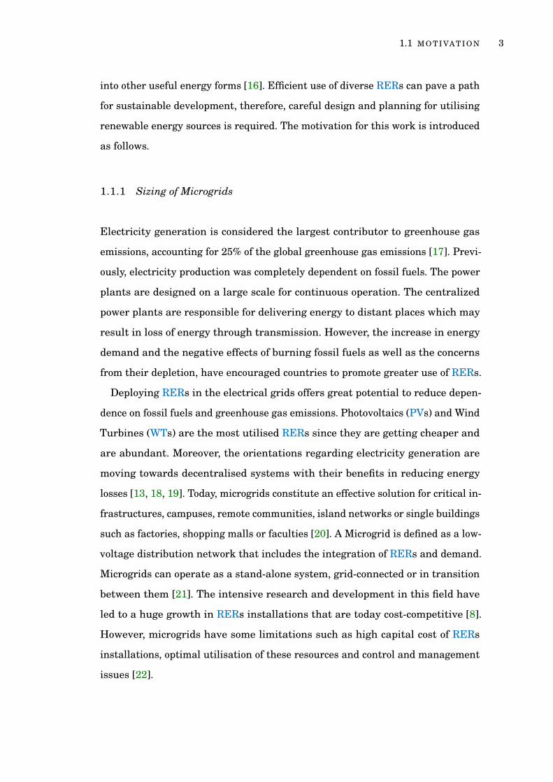
1.1.1 Sizing of Microgrids
Electricity generation is considered the largest contributor to greenhouse gas
emissions, accounting for 25% of the global greenhouse gas emissions [17]. Previ-
ously, electricity production was completely dependent on fossil fuels. The power
plants are designed on a large scale for continuous operation. The centralized
power plants are responsible for delivering energy to distant places which may
result in loss of energy through transmission. However, the increase in energy
demand and the negative effects of burning fossil fuels as well as the concerns
from their depletion, have encouraged countries to promote greater use of RERs.
Deploying RERs in the electrical grids offers great potential to reduce depen-
dence on fossil fuels and greenhouse gas emissions. Photovoltaics (PVs) and Wind
Turbines (WTs) are the most utilised RERs since they are getting cheaper and
are abundant. Moreover, the orientations regarding electricity generation are
moving towards decentralised systems with their benefits in reducing energy
losses [13, 18, 19]. Today, microgrids constitute an effective solution for critical in-
frastructures, campuses, remote communities, island networks or single buildings
such as factories, shopping malls or faculties [20]. A Microgrid is defined as a low-
voltage distribution network that includes the integration of RERs and demand.
Microgrids can operate as a stand-alone system, grid-connected or in transition
between them [21]. The intensive research and development in this field have
led to a huge growth in RERs installations that are today cost-competitive [8].
However, microgrids have some limitations such as high capital cost of RERs
installations, optimal utilisation of these resources and control and management
issues [22].

1.1 M O T I VAT I O N 4
Annual Installations (GW)
ROW
Middle East
LatAm
Germany
Japan
India
China
USA
2020
105
89
76
64
55
47
41
3331
202020192018201720162015201420132012
Figure 1.1: The evolution of global total PV installed capacity from 2012 to 2020 [1].
Among various RERs, PVs prove to be the most attractive option for electricity
generation. This is due to their benefits such as noiseless, environmental advan-
tages, simple operation and maintenance, and long lifespan [16]. Moreover, the
PVs cost is currently on a fast reducing track and will continue decreasing for
the coming years [23]. For these reasons, the RER under consideration in this
thesis is PV. Figure 1.1 shows the fast growth of the PVs installations (in GW)
applied widely in many countries from 2012 to 2020 [1]. The installed capacity
of PVs has increased from 2012 to 2016 by 24 GW, while from 2016 to 2020 this
value has doubled (50 GW).
Therefore, there is a genuine need to find the optimal sizing of the integrated
RERs and Energy Storage System (ESS). The importance of ESSs emerges from
their benefits in reducing the intermittent characteristics of the RERs. Find-
ing the sizes of the microgrid assets represents the first step in designing any
microgrid and is essential to mitigating the limitations of microgrids. Further-
more, the coordination between the integrated assets in microgrids represents

1.1 M O T I VAT I O N 5
a challenging task in designing microgrids. This is introduced in the following
section.
1.1.2 Energy Management Strategies
It is fundamental in designing any microgrid to obtain the sizes of the integrated
assets. However, the optimal operation of the microgrid and the coordination
between all the assets are also essential in every microgrid. One of the most
promising means of reducing energy consumption and related energy costs while
ensuring continuous demand supply is implementing an efficient Energy Man-
agement Strategy (EMS) [24]. An optimal microgrid sizing together with an
appropriate EMS determines the overall system performance and both deserve
similar attention.
The integration of RERs and ESSs in microgrids brings challenges to the
operation and stability of the grid [22, 25, 26, 27]. Therefore, a proper control
strategy is essential to ensure a smooth transition of energy in microgrids [27].
There are two essential options in controlling any microgrid; power management
control and EMS. In power management strategies voltage, current and frequency
are the main variables to consider. While in EMSs, the key parameters to optimise
are the cost, fuel cost, maintenance cost, and the system lifetime [28]. The EMS
serves several vital purposes such as [22]: (i) protects the ESSs by controlling the
charging and discharging cycles, (ii) ensures maximum utilisation of RERs, (iii)
ensures the continuous supply to the demand, (iv) and minimises the operation,
maintenance, fuel and replacement costs by efficient use of all the assets in the
microgrid. This thesis is interested in optimising the EMS along with the size.
The basic principle of existing optimisation approaches for microgrids are
either determining the optimal size [29, 30, 31, 32] or obtaining the optimal
EMS [33, 34, 35]. Few approaches tackled optimising both the size and EMS [36,
37, 38]. While these optimisation approaches have made piecemeal advances in
different directions, they leave room for further improvements. For example, how
1.2 T H E S I S S C O P E A N D C O N T R I B U T I O N S 6
to redefine the optimal size-EMS by implementing various EMS, and how the
obtained EMS can adopt any future changes and disturbances in the input data.
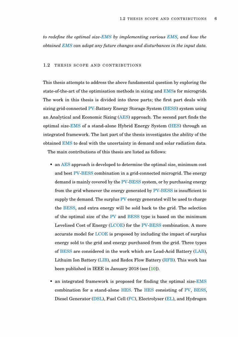
1.2 T H E S I S S C O P E A N D C O N T R I B U T I O N S
This thesis attempts to address the above fundamental question by exploring the
state-of-the-art of the optimisation methods in sizing and EMSs for microgrids.
The work in this thesis is divided into three parts; the first part deals with
sizing grid-connected PV-Battery Energy Storage System (BESS) system using
an Analytical and Economic Sizing (AES) approach. The second part finds the
optimal size-EMS of a stand-alone Hybrid Energy System (HES) through an
integrated framework. The last part of the thesis investigates the ability of the
obtained EMS to deal with the uncertainty in demand and solar radiation data.
The main contributions of this thesis are listed as follows:
• an AES approach is developed to determine the optimal size, minimum cost
and best PV-BESS combination in a grid-connected microgrid. The energy
demand is mainly covered by the PV-BESS system, or by purchasing energy
from the grid whenever the energy generated by PV-BESS is insufficient to
supply the demand. The surplus PV energy generated will be used to charge
the BESS, and extra energy will be sold back to the grid. The selection
of the optimal size of the PV and BESS type is based on the minimum
Levelised Cost of Energy (LCOE) for the PV-BESS combination. A more
accurate model for LCOE is proposed by including the impact of surplus
energy sold to the grid and energy purchased from the grid. Three types
of BESS are considered in the work which are Lead-Acid Battery (LAB),
Lithuim Ion Battery (LIB), and Redox Flow Battery (RFB). This work has
been published in IEEE in January 2018 (see [10]).
• an integrated framework is proposed for finding the optimal size-EMS
combination for a stand-alone HES. The HES consisting of PV, BESS,
Diesel Generator (DSL), Fuel Cell (FC), Electrolyser (EL), and Hydrogen

1.2 T H E S I S S C O P E A N D C O N T R I B U T I O N S 7
Tank (HT). In the first step, the proposed framework is used to determine
the size of the assets in the HES based on an initial EMS. Then the obtained
size is exercised through multiple EMSs produced using Finite Automata
(FA). This is followed by an evaluation model to compare the performance
indices of each instantiated EMS. The role of the evaluation model is to
track the featured operating conditions in the instantiated EMSs. Then
select the featured conditions that lead to an improvement in performance
indices and retain them in the new EMS. As such, the new-optimised
EMS will then replace the initial one leading to the optimal size-EMS
combination. The novelty in this work can be summarized as taking the
impact of selecting the right EMS on the sizing of the HES. This can lead
to better performance and can be explained in our integrated framework by
reducing the cost, reducing the DSL and FC working hours and increasing
the PV utilisation. Moreover, using FA in implementing and instantiating
multiple EMSs to attain an improved one has not been reported. This work
has been published in Applied Energy/Elsevier in May 2019 (see [39]).
• a Fuzzy Logic Controller (FLC) is implemented for the purpose of modifying
the selected EMS from the integrated framework. The main objective of
this FLC is to maintain the HES performance under uncertainty in demand
and solar radiation. A sensitivity analysis is conducted, and all possible sce-
narios are generated by making changes to the demand and solar radiation
data. These scenarios are utilised as input to the FLC, and the fuzzy sets
are the working hours of the DSL, fuel cost, and PV contribution. The fuzzy
output sets of FLC represent condition sets that will cause modifications on
the DSL, FC, and EL operating conditions in the original EMS. An article
has been prepared for this work, and it is under submission to Applied
Energy/Elsevier.

1.3 T H E S I S OV E R V I E W 8
1.3 T H E S I S OV E R V I E W
This thesis is organized into six chapters. The major contributions of this thesis
are summarized as follows:
Chapter 2 presents an essential background on microgrids, their benefits and
drawbacks, microgrids modes, and an illustration example of a microgrid consists
of RERs, DSLs and BESS. Then an introduction on ESSs is provided showing
the existing types of ESSs. The concept of HESs is introduced demonstrating
an example of their general architecture. This is followed by an investigation of
current EMSs in the literature up to date. Criteria for microgrid optimisation
and the sizing methods used for the sizing are also discussed.
Chapter 3 proposes an AES approach for sizing a grid-connected PV-BESS.
It demonstrates how the analytical models of the PV and BESS are employed
with the LCOE model to optimise the size of the PV-BESS. Moreover, the LCOE
model is modified from its original form to include the cost of the surplus energy
sold to the grid and energy purchased from the grid. A comparison between the
combinations of PV-BESS obtained by the AES approach is performed to show
the effect of the LCOE on selecting the best combination.
Chapter 4 demonstrates an integrated framework for sizing a stand-alone
HES. It describes the steps of the integrated framework in detail. A modified
version of the AES approach implemented in Chapter 3 is used in the first step
of the framework. The utilisation of FA in the framework to implement and
generate multiple EMSs is also discussed. The evaluation model used to assess
the instantiated EMSs and to select the featured conditions is explained. The
process of resizing with the improved EMS is clarified and the obtained results
from the AES and the framework are compared.
Chapter 5 investigates the effect of the demand and solar uncertainty on the
performance of the HES introduced in Chapter 4. It shows how the system is
resized using AES approach and forecasted data for demand and solar radiation.
It introduces all possible sensitivity analysis scenarios for the new size of the
HES. This chapter demonstrates how the obtained sensitivity scenarios are

1.3 T H E S I S OV E R V I E W 9
utilised to perform a FLC. It explains how this FLC is designed in detail, and its
application to modify the EMS. Moreover, a case study of one of the sensitivity
analysis scenarios reporting the results after and before applying the FLC is
discussed.
Chapter 6 summarizes the contributions and key highlights of this thesis, show-
ing critical review of this research together with the potential future directions.
Overall, this thesis shows promising design and implementation approaches
for finding the optimal size and EMS of microgrids. It can provide an addition to
the existing literature in the field of optimisation of microgrids.

2
BA C K G R O U N D A N D L I T E R AT U R E S U R V E Y
2.1 I N T R O D U C T I O N
The drivers of integration RERs in microgrids is to combat climate change,
environmental pollution, and increasing global demand. WT, PV, hydropower,
geothermal energy, and biomass energy are examples of RERs. PV is one of the
fastest growing technologies and widely applied in many countries. It is expected
in the coming decade the PV installations in the world will be approximately
doubled [40]. Efficient use of various RERs allows for more sustainable energy
systems. As a consequence, design and planning for utilising RERs in microgrids
are required.
This chapter highlights the basic concepts raised in the field of microgrids
to understand the state of the art reported in the context of this work. First,
the concept of microgrid and the assets that contribute to the microgrid is ex-
plained. Then the, multiple criteria for microgrid assessment are introduced to
determine which RER and EMS are better to use. Following that, the importance
of controlling and managing microgrids is clarified. Since microgrid design is
the primary theme of this thesis, the second part of this chapter is made to
emphasize the research efforts in the field of sizing methods found so far and its
classification. Finally, a discussion is placed for the comparison between all the
available methods.
2.2 M I C R O G R I D S
During the past decades, the deployment of Distributed Generations (DGs) in
the existing power systems has been increasing rapidly. DG refers to any small-
10

2.2 M I C R O G R I D S 11
scale power system that operates independently of the utility grid and located
on the user side where it is utilised [41]. DGs include RERs such as PVs and
WTs, and Alternative Energy Resources (AERs) such as FCs and Microturbiness
(MTs)s [13, 22, 42]. In addition, DGs include non-renewable generators such as
DSLs and gas turbines [43]. Microgrid has emerged as an attractive option to
harness the benefits offered by the DGs to the existing power systems [44, 45]. The
U.S. Department of Energy defines a microgrid as "a group of interconnected loads
and distributed energy resources within clearly defined electrical boundaries
that acts as a single controllable entity with respect to the grid. A microgrid can
connect and disconnect from the grid to enable it to operate in both grid-connected
and island mode [46]." Island or stand-alone microgrid are two terms for the
same concept, the term stand-alone will be used in this thesis.
2.2.1 Microgrid Benefits and Drawbacks
The intuitive advantages of microgrids have been broadly classified into envi-
ronmental and economical benefits. However, other advantages of microgrids
are represented in a significant reduction in energy losses and improvement in
the utilisation of RERs. The reliability of the systems is also improved by con-
necting multiple generating units to ensure continuous demand supply. Also, the
decentralization of DGs allows the microgrid in the cases of outages to operate
independently leading to a reduction in the adverse effects of outages. Moreover,
one of the advantages of microgrids is to enhance EMS by properly matching
the supply and demand to reduce the energy imported from the grid. [47, 48, 49].
Figure 2.1 shows an example of a microgrid that includes a PV farm, WT farm,
various demand, DSLs and BESS. The presented microgrid can operate in both
modes, stand-alone and grid-connected through the point of common coupling. In
grid-connected mode, the PVs and WT will supply the residential and industrial
demand during their availability. The BESS will store surplus energy from WT
to supply when needed. However, any deficiency in energy will be covered by the

2.2 M I C R O G R I D S 12
Grid
Wind
turbine
Battery
Energy
Storage
System
Industrial
demand
Residential
demandPhotovoltaic
Residential
demand
DSL
Point of
common
coupling
DSL
Photovoltaic
Figure 2.1: Example of a microgrid including PV, WT, BESS, DSL for a residentialand industrial demand. The presented microgrid can operate in both grid-connected and stand-alone modes.
grid. In stand-alone mode, the DSLs acts as a backup generator and supply the
demand.
In addition, RERs and AERs are environmentally friendly, these energy re-
sources will never die out as they are continuously replenished. However, because
of the stochastic and intermittent nature of RERs, affording continuous elec-
tricity from a power system with integrated RERs presents a challenge. One of
the most efficient technologies providing anticipated unit cost reductions, which
makes the investment in RERs/AERs looks extremely attractive, is ESSs. The
integration of ESS along with RERs/AERs is assumed to provide fundamental
advantages to the microgrid. This is represented by maintaining the balance
between generation and consumption, and improving the reliability of the power
grid [50]. Section 2.3 explains the benefits of ESSs in more details.
Another practical solution to overcome the intermittency of RERs is HESs. A
HES combines two or more RERs with some conventional source like DSL along
with an ESS (HESs are explained in Section 2.4).
To determine the optimal exploitation of RERs/AERs in microgrids, the system
design must consider significant factors. These factors relate to the operation,

2.2 M I C R O G R I D S 13
component selection, and applied methodology. Therefore, choosing an optimum
sizing methodology is fundamental to meet the desired demand at a distinct level
of security. Sizing and optimisation techniques allow the power system to operate
efficiently and economically in different conditions [51], and Section 2.8 discusses
the available sizing methods in the literature.
Stability and protection in microgrids are also issues that need to be investi-
gated when integrating DGs in the electrical grid. However, these issues are out
of the scope of this thesis.
2.2.2 Microgrids Modes
Whether a power system is based on single RER/AER or a HES, it can be con-
figured either to be stand-alone or grid-connected. The selection of the possible
configuration depends on key parameters: (i) the possibility of grid extension, (ii)
the electricity cost of energy supplied from the grid and, (iii) the weather fore-
casting in the specific area. Grid-connected configurations are typically preferred
for applications in urban areas, while stand-alone configurations may be suitable
for remote locations [51].
The main priority of grid-connected microgrids is to cover local demand from
available RERs/AERs; any surplus energy will be fed into the grid. In the case
where there is a shortage of electricity, it will be drawn from the grid. In grid-
connected systems, the grid acts a backup source. On the other hand, stand-alone
microgrids produce energy independently from the grid, where DSLs can be used
as a backup source. These systems are preferable for remote areas where the grid
cannot penetrate and there is no other source of energy [18, 22].
A comparison between grid-connected and stand-alone microgrids, on which the
decision of which mode to consider in the microgrid, is presented as follows [18]:
• The accessibility of the location where DGs installed, grid-connected sys-
tems are ideal for locations near to the grid where the grid extension is
convenient. The stand-alone systems are suitable for remote areas because

2.3 E N E R G Y S T O R A G E S Y S T E M S 14
of the irregularities in the topological structure of the area and the distance
which makes the connection to the grid very difficult [51].
• The economic feasibility is critically important in deciding whether to make
the system grid-connected or stand-alone. In grid-connected systems, the
surplus energy will be used either to charge a battery or be fed back into
the grid, which will be more profitable than stand-alone systems.
• The connectivity to the grid enables grid-connected systems to set up large-
scale systems with high plant load factors (where a high load factor means
that power usage is relatively constant) thereby improving the economic
viability of the operation. On the other hand, stand-alone systems are
required to operate with low plant load factors (low load factor shows that
occasionally a high demand is set).
• In grid-connected systems the grid acts as a back-up for the system, accord-
ingly increasing its efficiency. While the back-up in stand-alone systems
could be an ESS or small-scale distributed generator.
• If the grid-connected system is incorporated with an ESS, it will be cost-
effective by reducing the energy imported from the grid while selling the
surplus energy to the grid. In stand-alone systems, the excess energy will
be discarded, which will be considered as energy loses.
2.3 E N E R G Y S T O R A G E S Y S T E M S
The ESS refers to the process of converting electrical energy from a power system
into a form that can be kept in various types of storage. Then the stored energy can
be used when needed by transforming it back to serve the intended purpose [52].
ESS technologies have been found to be the best solution for the challenges
associated with the proliferation of DGs. An ESS has multiple functions when
installed in a distribution system, and some of these functions can be summarised
as follows [50, 53, 54, 55]:

2.3 E N E R G Y S T O R A G E S Y S T E M S 15
• To facilitate the integration of the RERs into the grid, increasing their
penetration rate, and enhance the quality of the energy supplied.
• To reduce peak demand problems by providing energy when needed and
hence eliminating the extra operation of the traditional generators (such as
DSL) during the peak periods.
• To provide a balance between generation and consumption and improving
the management and reliability of the grid.
• To provide remote areas with their energy needs, in cases when it is chal-
lenging to set up new grid connection plans.
• To reduce the energy imported from the electrical grid in grid-connected
systems.
• To improve the electrical system’s overall stability and making the elimina-
tion of power disturbances possible.
Many ESS technologies are available in the market, and the selection of the
appropriate storage technology depends on several factors. Power rating, dis-
charge time, suitable storage duration, lifetime, life cycle cost, capital cost, round
trip efficiency, and maturity represent the key factors in selecting the appro-
priate ESS [56]. ESSs can be categorized into: electrical, mechanical, thermal,
electromechanical, magnetic, chemical and thermochemical [55, 57, 58, 59, 60],
and Figure 2.2 shows different types of ESSs and examples on each type. Elec-
trochemical BESS technologies, namely lead acid (LA), nickel-cadmium (NiCd),
nickel-metal hydride (Ni-MH), lithium ion (Li-ion), and sodium-sulfur (NaS)
batteries are widely used in microgrid energy systems [50]. Detailed reviews of
ESS technologies can be found in [50, 55, 56].

2.4 H Y B R I D E N E R G Y S Y S T E M S 16
Energy storage systems
Electrical
Capacitors
Supercapacitors
Mechanical
Compressed air
Pumphydro
Thermal
Hot water
Ceramic thermal storage
Thermal fluid
Electromechanical
Batteries
Flow batteries
Magnetic
Superconducting
Magnetic energy storage
ChemicalThermo-
chemical
Hydrogen
Synthetic
natural gas
Batteries
Ammonia
and water
Magnesium
sulphate
Figure 2.2: Types of ESSs used in microgrids and examples for each type.
2.4 H Y B R I D E N E R G Y S Y S T E M S
RERs include among others PV, WT, and tidal. However, utilising PV energy
gained more attention than others for many reasons: (i) infinite, (ii) needs mini-
mal maintenance, and (iii) the running costs are extremely small and have zero
carbon emissions [61]. To obtain the maximum benefits of solar energy or any
other RERs, hybridization has emerged. A hybrid energy system (HES) combines
two or more of RER/AER to feed a required demand and may include conventional
energy resources and ESSs [62, 63, 24]. The primary role of the HES is to ensure
maximum production of energy while maintaining the quality and continuity of
the provided service [64]. Despite the unpredictable nature of RERs, introduc-
ing HES can present complementary patterns such that each resource provides
energy if the other resources are unavailable. HES considered the most efficient
option where grid connectivity is practically impossible or uneconomical [65].
Figure 2.3 demonstrates a general architecture of the HES.
The HES can be configured as grid-connected or stand-alone systems. The
grid-connected HESs are designed in a way that the participating resources can
cover the local demand, and any surplus energy will be stored or sold to the grid.
In addition, installing ESSs in the grid-connected HES is not a necessity as the
grid acts as a backup system. Whereas the stand-alone HESs need ESSs to store

2.5 C R I T E R I A F O R M I C R O G R I D O P T I M I S AT I O N 17
Renewable energy
resource 1
Renewable energy
resource 2Control Unit
DC/AC
inverterDC loads AC loads
Renewable energy
resource 3
Energy storage
System 1
Energy storage
System 2
Conventional
energy
System 1
Electric
Grid
Figure 2.3: General architecture of HES that shows the diversity in the assets such asRERs, inverters, AC demand, DC demand, ESSs and control unit represent-ing the energy management strategy.
the surplus energy and a backup system such as DSLs to maintain continuity of
service.
On the environmental level, HESs can reduce the emissions of greenhouse
gas through the increased use of RERs [66]. Moreover, it has been demonstrated
that HESs can significantly reduce the total life-cycle cost of stand-alone systems
in many situations, while at the same time providing a more reliable supply of
electricity [63].
To obtain the best performance of HESs in terms of maximising the utilisation
of the generated energy and minimizing the total cost, two crucial issues are
considered: appropriate sizing and suitable energy management strategy [67, 68,
69]. These two issues are considered in this thesis.
2.5 C R I T E R I A F O R M I C R O G R I D O P T I M I S AT I O N
The key objective of introducing microgrids with RERs/AERs is to satisfy the
demand requirements at any time taking into consideration the growing demand
and this is the reliability assessment. The economic side is also very important
2.5 C R I T E R I A F O R M I C R O G R I D O P T I M I S AT I O N 18
in microgrid optimisation, in order to reach to the most cost-effective microgrid.
Additionally, the environmental aspect is very essential to reduce global warming.
Therefore, reliability, economics and environmental assessment are fundamental
in any microgrid design [70].
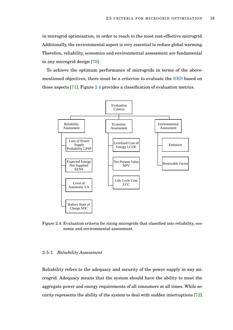
To achieve the optimum performance of microgrids in terms of the above-
mentioned objectives, there must be a criterion to evaluate the HES based on
those aspects [71]. Figure 2.4 provides a classification of evaluation metrics.
Evaluation Criteria
Reliability Assessment
Expected Energy Not Supplied
EENS
Level of Autonomy LA
Battery State of Charge SOC
Economic Assessment
Levelized Cost of Energy LCOE
Net Present Value NPV
Life Cycle Cost LCC
Environmental Assessment
Emission
Renewable Factor
Loss of Power Supply
Probability LPSP
Figure 2.4: Evaluation criteria for sizing microgrids that classified into reliability, eco-nomic and environmental assessment.
2.5.1 Reliability Assessment
Reliability refers to the adequacy and security of the power supply in any mi-
crogrid. Adequacy means that the system should have the ability to meet the
aggregate power and energy requirements of all consumers at all times. While se-
curity represents the ability of the system to deal with sudden interruptions [72].

2.5 C R I T E R I A F O R M I C R O G R I D O P T I M I S AT I O N 19
There are several reliability indicators for microgrids that can asses their perfor-
mance, and some of these are given below [73]:
• Loss of Power Supply Probability (LPSP): an electrical system is reliable
when it is capable to supply enough power to the demand during a certain
period. The most reliable indicator for that is the LPSP defined as the ratio
of energy deficiency to demand during a certain period. The lower LPSP
the more reliable operation of the power system, if LPSP equals zero means
the installed DGs can cover the demand. Whereas if the LSPS is one, this
indicates the demand is never fed [74]. Generally, LPSP is calculated as
follows [73]:
LPSP =∑T
t=1 DE(t)∑Tt=1 Pload(t)
, (2.1)
where DE(t) and Pload(t) represent the deficiency in energy and the demand
during a certain time respectively.
• Expected Energy Not Supplied (EENS): this indicator measures the ex-
pected energy that cannot be supplied when the demand exceeds the avail-
able energy in the system. EENS can be obtained as follow [74, 73, 75]:
EENS =
Pload −∫ Pmax
PminP . fP (P) dP Pload > Pmax∫ Pmax
Pmin(Pload −P) . fP (P) dP Pmin ≤ Pload ≤ Pmax
0 Pload ≤ Pmin
, (2.2)
where P is the power generated by the microgrid, Pload refers to the de-
mand, fP (P) is the probability density function for the power output of the
microgrid. While Pmax and Pmin are the maximum and minimum power
generated by the microgrid respectively.

2.5 C R I T E R I A F O R M I C R O G R I D O P T I M I S AT I O N 20
• Level of Autonomy (LA): this indicator is defined as one minus the ratio
between the total number of hours in which loss of load HLOL occurs and
the total hours of operation Htot [73]:
LA = 1− HLOL
Htot, (2.3)
where HLOL represents the number of hours for which loss of load occurs
and Htot is the total operating hours of the system.
• Battery state of charge (soc): soc is related to the energy stored in the
battery. It can help in determining the battery capacity to ensure that the
constraints about system reliability are met and can be calculated using
the following equation:
soc(t)=
soc(t−1)+ [Pinput(t)−Pload(t)] ·ηch ·∆tηinv · BatC
, Pinput(t)> Pload(t) ,
soc(t−1)− (Pload(t)−Pinput(t)) ·∆tηinv ·ηdch ·BatC
, Pinput(t)≤ Pload(t),
(2.4)
where Pinput is the sum of input power to the battery, Pload represents the
demand, BATC is the battery capacity in kWh. Whereas ηinv, ηch, and ηdch
are the inverter, battery charging and discharging efficiency respectively.
∆t is the time interval between this state and the previous one.
2.5.2 Economic Assessment
Economic analysis is essential for any power system and has a strong relationship
with power system reliability. The inadequate reliability of power supply costs
customers much more than adequate reliability [76]. It will be noted in the
following section, that almost all sizing methods use economic assessment to

2.5 C R I T E R I A F O R M I C R O G R I D O P T I M I S AT I O N 21
obtain the optimal size of the assets in a microgrid. Underneath are some of the
economic indicators used to determine the economic feasibility of a power system:
• LCOE: is widely used to evaluate the economic feasibility of power systems
and ESSs. The costs distributed over the project lifetime are considered
and this provides a more accurate economic picture of the project under
analysis [77, 78, 79]. The LCOE of the microgrid can be obtained by dividing
the total cost of the assets in the microgrid by the total energy generated.
Equation 2.5 represents the general form of LCOE [10]:
LCOE = Total S ystem CostsTotal Annualized Energy Production
(£/kWh) , (2.5)
• Life Cycle Cost (LCC): is the total system cost calculated during the lifetime
of the system. The LCC consists of three components, which represent the
initial cost (ICsystem), the annualized replacement cost (RCsystem), and the
annualized operation and maintenance cost (OMsystem) [80]. It is calculated
as follows:
LCC = ICsystem +OMsystem +RCsystem . (2.6)
• Net Present Value (NPV): the NPV of a power system is the difference
between the present values of the total profit and total cost of the system
within its operational lifetime. Obviously, the higher the NPV, the higher
economic benefit [81].
2.5.3 Environmental Assessment
Environmental assessment is a vital aspect of sustainability, that causes a di-
rect effect on our planet. Environmental assessment is related to reducing the
pollution that could result from some DGs. Two important indicators in the
environmental assessment are emissions and the renewable factor.

2.6 C O N T R O L A N D E N E R G Y M A N A G E M E N T O F M I C R O G R I D S 22
• Emission: the emissions of a microgrid include carbon dioxide (CO2), sul-
phur dioxide (SO2) and nitrogen oxides(NOx). Based on the Tokyo Protocol,
CO2 and NOx are two types of the six main greenhouse gases. SO2 is one
of the most primary reasons for acid rain. The emissions of any microgrid
are measured as yearly emissions of the emitted and the emissions into the
air of different systems [72].
• Renewable Fraction: the renewable fraction means the amount of renewable
energy generated divided by the total energy generated by the system, and
it represents the extent of renewable energy in a microgrid. A higher value
of this factor indicates that a great portion of RERs is used [72].
2.6 C O N T R O L A N D E N E R G Y M A N A G E M E N T O F M I C R O G R I D S
Microgrid control is responsible for dealing with multiple aspects such as the
voltage and frequency regulation, irregularity of the RERs, the imbalance be-
tween demand and generation, and the type of the integrated ESS [82, 83, 84].
The diversity in control issues led to the adoption of the hierarchical control
scheme as a standardized solution in microgrids, especially when different time
processing is required to execute the multiple tasks [82, 83]. Generally, the con-
trol in microgrids can be divided according to the hierarchical control into three
levels. The primary level is responsible for local control of DGs, the secondary
level deals with the frequency and voltage deviations. Finally, the tertiary level
is identified as the EMS where it is responsible for managing the power and the
energy between DGs and the demand. The scope of this thesis is oriented towards
the third level of control [84, 83].
When combining one or more of RERs/AERs along with an ESS to supply a
certain demand, the need for an effective EMS arises [85]. EMS represents a
sequence of instructions to determine decisions regarding the operation of the
assets in the microgrids and to guide the flow of energy in the microgrid. The
need for an EMS is fundamental for both grid-connected and stand-alone systems.

2.6 C O N T R O L A N D E N E R G Y M A N A G E M E N T O F M I C R O G R I D S 23
The role of the EMS differs based on the microgrid configuration. For instance, in
grid-connected systems the EMS controls the energy flow to and from the grid.
However, in stand-alone systems, the EMS role is to ensure continuity of supply
to the demand, improve the system performance, maximise the utilisation of
RERs, reduce the system operation cost, and prolong system lifetime [25].
A generalized structure of EMS is presented in Figure 2.5. A typical EMS
requires data input such as components costs, fuel price, demand and RERs pro-
files, and the assigned objectives. There are three types of microgrid assessment
which are reliability, economic and environmental (explained in Section 2.5). The
assessments are considered as objectives for EMS optimisation. Accordingly, the
EMS provides output information such as the decision which DGs to operate,
when to charge/discharge the ESS, whether to import/export energy from the
grid. Moreover, indices to evaluate the microgrid performance are produced by
the EMS.
EMS
Operation of DGs
Performance evaluation
Import/export energy from the
grid
(grid-connected Microgrid)
Demand/RERs profiles
Operational objectives
DGs cost and fuel price
Figure 2.5: Energy Management System.
The EMS of a microgrid is a research topic widely tackled in literature in the
past few years. In this thesis, the EMSs are classified into two groups based on

2.6 C O N T R O L A N D E N E R G Y M A N A G E M E N T O F M I C R O G R I D S 24
the algorithm or method used to implement the EMS. The two groups are EMSs
based on classical approaches and EMSs based on intelligent approaches.
• EMSs based on classical approaches
The EMS implemented by classical approaches is known for its simplicity in
term of control and design. These approaches include rule-based, linear and
nonlinear programming. Rule-based EMSs are governed by a series of rules
and they are widely used due to their simplicity and practicality [22]. In [37],
three rule-based EMSs are developed to find the size and suitable EMS
for a stand-alone HES. The HES consists of PV, BESS, FC, EL, and HT.
The three EMSs were designed based on operating modes and combining
technical-economic aspects. The objective of the EMSs were mainly to
satisfy the demand, then, maintain a certain level in the HT and BESS.
Linear programming is one of the simplest methods for determination of the
optimal solution in problems with several alternative solutions. The method
is based on maximising or minimising an objective function according to
constraints and bounded variables to obtain the unknown parameters.
Nonlinear programming is the same as linear but the objective function
contains a nonlinear function [86]. For example, linear programming was
used to develop an EMS for a HES [87]. The objective of the EMS was
to minimise the operation cost of the HES. The cost function integrates
all associated degradation costs and the lifetime of all the assets in the
HES. The HES includes PV, WT, FC, EL, and HT. The results showed an
improvement of the EMS against conventional EMS.
In general classical approaches are easy to implement and understand
and commonly used in the literature. Nevertheless, these methods are not
suitable for big and complex systems where the complexity and calculation
time of the overall optimisation procedure are increased.
• EMSs based on intelligent approaches
Recently, many studies have been conducted on EMS using Artificial Intelli-
gence (AI) techniques, such as Genetic Algorithim (GA), artificial neural net-

2.7 FI N I T E AU T O M ATA A N D F U Z Z Y L O G I C 25
work, particle swarm optimisation as well as hybrid approaches [22, 24, 88].
Implementing EMSs using AI approaches lead to enhance the efficiency
and performance of microgrid and thereby meet the demand with maximum
energy production [27]. Additionally, AI approaches are able to deal with
nonlinear systems and multi-objective systems efficiently. However, the
execution time for these approaches maybe longer in some cases and achiev-
ing a real-time control may not be possible [27]. Moreover, AI approaches
require enough knowledge and experience for systems to be implemented
efficiently.
A GA-memory based EMS is presented by Azkarzadeh [89] for optimal
sharing of the power generation task between the DGs in a grid-connected
microgrid. The objective of the EMS was to minimise the operating costs of
PV, WT, and combined heat and power system. A multi-objective particle
swarm optimisation EMS is introduced by Manbachi et al. [90] for real-time
managing of a stand-alone microgrid. A new concept called the operation
value factor was defined for each objective function to minimise the micro-
grid load shedding and increase achieve higher levels of performance and
reliability.
2.7 FI N I T E AU T O M ATA A N D F U Z Z Y L O G I C
This section introduces FA which represents a mathematical model of computing
used in the design of many computer hardware and software [91]. FA is used
for implementing multiple EMSs within the integrated framework in Chapter 4.
The application of FA in power systems application is also presented. Moreover,
an introduction on FLC and its application in a microgrid is presented.

2.7 FI N I T E AU T O M ATA A N D F U Z Z Y L O G I C 26
2.7.1 Finite Automata and Discrete Event Systems
Discrete Event Systems (DESs) are discrete-state, event-driven systems among a
set of finite states, with an initial state and one or more of marked states [92, 93].
Traditionally, regular languages and finite automata have been used both for
modelling and analysis of DESs in the supervisory control community [94].
The first application of DESs in the power system was in 1995, where Prosser
et al. [95] modeled a 14-bus 40-line transmission network using DES. Two states
were considered for each line: line in service and line out of service. While
the events that triggered the system are: line restoring and line tripping. The
Supervisory Control of Discrete Event Systems (SCDES) was designed to manage
the restoring operation of tripping lines with a high level of security. In a similar
fashion, Lee et al. applied SCDES to obtain the restoration strategies for the
power distribution networks, while maintaining a high level of security and satis-
faction of the demand [96]. Another work of utilising DES was done by Afzalian
et al [97, 98]. The SCDES was applied for the operation of the tap-changing
transformer, and dynamic flow controllers. The components were modeled using
Automata and synthesized using TCT software [99]. In [100], Kharrazi et al.
investigated the application of SCDES to a custom power park. The components
in the CPP were modeled using Automata, synthesized using the TCT software
and simulated using MATLAB/Simulink. Recently, Sadid et al. [101] presented
the scheduling of thermal devices operation in the framework of DESs. Two
algorithms were developed to reduce the peak demand, and the results showed a
noticeable improvement in peak demand reduction. In this thesis, FA are used
to implement an EMS. Modelling the EMSs using FA has many advantages in
terms of reducing the complexity of the system, a better understanding of the
microgrid. As well as, facilitate the adding or changing of the operating conditions
(conditions responsible for the operation of a certain asset in the microgrid), and
increasing the ability to accommodate new assets smoothly.

2.7 FI N I T E AU T O M ATA A N D F U Z Z Y L O G I C 27
2.7.2 Fuzzy Logic
The FLC is a flexible tool with rules based on human knowledge and experience.
The uncertainty in the input variables can be handled efficiently by the FLC.
Moreover, FLC is very suitable for complex models, such as HES [102]. The
success of FLC is due to their ability to deal with the knowledge represented in a
linguistic form instead of the conventional mathematical method [103].
The FLC follows three basic steps [104, 103]; the first step is converting the
inputs into fuzzy values as a degree of membership of fuzzy sets. This membership
function is a curve that defines how each point in the input space is mapped to
membership value or degree of membership between 0 and 1. This step is called
fuzzification. The second step is to link the controller output to the inputs using
a list of IF – THEN rules. A fuzzy IF – THEN rule represents an IF – THEN
statement in which some words are characterized by membership functions. The
IF part of a rule specifies the combination of inputs for which a rule holds. The
THEN part of a rule refers to values of the output variable [105, 106]. Finally,
converting the output fuzzy set into a particular value that can be used as an
output, which called defuzzification.
The FLC has been extensively used by researchers for several applications
in microgrids with RERs [107]. For example, implementing FLC-based EMS
for both grid-connected and stand-alone microgrids. A FLC was employed by
ArcosvAviles et al. [108] to implement an EMS in a grid-connected microgrid.
The microgrid consists of PV, WT, and BESS. The objective of the FLC-based
EMS was to achieve smooth power profile by minimising the fluctuations and
power peaks during the energy exchange with the grid. The FLC-based EMS also
proved to maintain the level of the BESS close to 75% leading to improvement in
the lifetime of the BESS. A FLC-based EMS was also presented by Kyriakarakos
et al. [109] for a stand-alone microgrid. The microgrid includes PV, WT, BESS,
EL, FC, HT, and water tank. The objective of the EMS was to minimise the Net
Present Cost (NPC) as well as the penalty cost on BESS, HT and water tank. The
demand divides into three types; electrical. hydrogen and water. The decision

2.8 M I C R O G R I D S S I Z I N G M E T H O D S 28
inputs for the FLC were the state of the charge for the BESS, water and system
frequency.
Implementing a Maximum Power Point Tracking (MPPT) for a PV system
based on FLC is also one of the applications of FLC in microgrids. Gheibi et
al. [110] utilised FLC to obtain the maximum power from PV. The objective of
the MPPT-based FLC was to minimise the uncertainties in the solar data. In
addition to the abovementioned applications, Macedo et al. developed a FLC
for the order of implementation of smart grid electrical systems [111]. The FLC
calculates a priority index which evaluates the energy systems to achieve the
best cost-benefit analysis.
2.8 M I C R O G R I D S S I Z I N G M E T H O D S
The key concept of system unit sizing is derived from the importance of opti-
mally managing all available assets and achieving suitable cost and reliability
levels. These mentioned objectives are commonly in conflict since sometimes
over-sizing the system will increase the total cost and under-sizing could cause
a system failure. Therefore, a reasonable trade-off is sometimes necessary to
design a reliable system with minimum costs [112]. Additionally, increasing the
number of components in the system to be optimised will increase the system
complexity, causing an increase in the time and effort required. Accordingly, it
is fundamentally significant to find an optimisation method to select optimum
system configurations readily and precisely.
Sizing methods of microgrids can be either a single objective or multi-objective
functions. Single objective function depends on determining the optimal size
depending on the minimum or maximum of a defined parameter. In contrast, the
multi-objective function uses more than one defined parameters to optimise the
microgrid size [113].
Finding the optimal sizing of the assets in a microgrid is an active research
area with extensive literature regarding this topic. It can be classified into seven
approaches, each one demonstrating a different technique to achieve the main

2.8 M I C R O G R I D S S I Z I N G M E T H O D S 29
objective of microgrid sizing. Figure 2.6 lists the sizing methods described in this
section.
Sizing Methods
Artificial Intelligence
Graphical Construction
Method
Analytical Method
Iterative Method
Probabilistic Methods
Hybrid Methods
Software Tools
Figure 2.6: Methods used for sizing microgrids with RERs and classified into sevenmethods.
2.8.1 Graphical Construction Methods
A graphical construction technique is based on a seasonal analysis that is made
for the variation in demand and resource availability during winter and summer
months. Due to this analysis, a sizing curve is developed between the various
sizes of wind turbines and PV generators available. If the data are collected for a
longer period, then a more refined curve is obtained.
Markvart [114] used the graphical construction method to determine the size
of a stand-alone HES consists of PV, WT, and BESS. The methodology based
on the situation where the average value of demand must be satisfied by the
average values of PV and wind power. Boroway et al. [115] developed a tech-
nique to find the optimum combination for a PV-WT system with a BESS for a
stand-alone HES. The procedure based on long-term meteorological data of PV
and wind profiles recorded each hour and each day for 30 years. These profiles
were used to obtain the average power generated by PV and WT. The calcula-
tion of the optimum number of PV modules and BESS was based upon LPSP
concept and minimum cost of the system. However, the main disadvantage of the
graphical construction method is that only two parameters can be included in
the optimisation process. For example, either PV and ESS or PV and WT can be
optimised [8, 71]. Additionally, these methods require long-term meteorological

2.8 M I C R O G R I D S S I Z I N G M E T H O D S 30
data to provide effective results. Basically, the graphical construction method
does not require an EMS, since the sizing is done by implementing a fitting curve
and based on the solution of the demand-supply criteria.
2.8.2 Analytical Methods
Analytical methods are computational methods that describe the system size as a
function of its techno-economic feasibility. In these methods, a series of steps need
to be followed in order to achieve the desired optimisation. Once the model is set,
system performance can be evaluated according to certain criteria [113, 73].
Khatod et al. [116] presented an analytical approach for a small autonomous
power system using WT and PV sources in Kandla, India. The objective of this
approach was to minimize the cost of the production. The simulation was per-
formed using the proposed analytical approach and Monte Carlo simulation, and
the obtained results were compared in terms of accuracy and computational time.
The analytical method showed less computational burden and time compared to
the Monte Carlo simulation, as well as less meteorological data needed.
Bortolini et al. [117] proposed an analytical method to find the techno-economic
sizing of a grid-connected PV-BESS. The analytical method determines the PV
rated power and the BESS capacity based on the minimum LCOE. The authors
employed the same analytical method to design a stand-alone HES with PV,
BESS, and DSL installed in a remote village in Yakutsk, Russia. For the latter
study, the analytical method used to calculate the carbon footprint of electricity.
The application of analytical methods is also presented by Kanase-Patil et
al. [118]. A methodology is developed to select and size different system com-
ponents, namely micro-hydropower, biomass, biogas, WT, PV, and BES. The
stand-alone system is designed to meet the electrical and cooking energy needs
of a cluster of villages in Uttarakhand state in India. The purpose of this study
was to determine the optimal combination of energy subsystems to minimize the
Cost of Energy (COE) generation and EENS.

2.8 M I C R O G R I D S S I Z I N G M E T H O D S 31
Hung et al. [119] presented an analytical method to obtain the optimal power
factor of each DG to reduce the energy losses. The analytical expression is based
on a multi-objective function, then the optimal location, size, and the number of
DGs are determined based on benefit-cost analysis.
In [120], Wissem et al. exploited mathematical models to determine the optimal
configuration of a stand-alone PV-ESS. The objective was to satisfy the require-
ments of a typical residential home located in Sfax, Tunisia. The optimising step
was performed based on lack of energy to generate probability, percentage of the
surplus of energy produced and the cost of the kilowatt-hour produced.
The system performance can be assessed in an accurate way with the use of an-
alytical methods. However, in case of multi-objective function optimisation, these
methods do not always offer accurate solutions. The analytical methods perform
well for small and simple systems; they are inappropriate for large and complex
systems [121]. For this type of optimisation, iterative, artificial intelligence and
hybrid methods provide better results for multi-objective functions [73]. As these
approaches can deal with non-linear behavior of systems’ components.
2.8.3 Iterative Methods
An iterative method represents a recursive process which stops when the best
configuration is reached according to the design specifications [6, 9, 74]. Iterative
methods have been extensively employed in the literature because of their ability
to deal with multi-objective systems.
Akram et al. [122] presented an optimal sizing of a WT, PV, and BESS grid-
connected HES. In this study, two iterative algorithms are implemented to find
the optimal sizing of the HES. The first algorithm finds the size of RERs, while
the second algorithm determines the size of the BESS. The optimisation of these
algorithms is based on maximum reliability and minimum cost.
A methodology to determine the optimal sizing of an autonomous hybrid PV-WT
system has also been suggested [123], in which accurate mathematical models for

2.8 M I C R O G R I D S S I Z I N G M E T H O D S 32
characterizing the PV module, WT and BESS were proposed. Then the optimal
sizing of the system was found according to minimising the LPSP and the LCOE.
Hosseinalizadeh et al. [124] presented an algorithm to optimise the size of
a stand-alone HES. The HES consists of PV, WT, BESS, and hydrogen system
where the fuel cell is treated as a backup system. The optimal size is based
on minimizing the system’s total cost for different four regions in Iran. The
authors assessed the reliability of the HES using less of load expectation and
loss of energy expectation. The study found HES is more economical and reliable
without a fuel cell.
Smaoui et al. [125] developed an iterative algorithm to find the optimal sizing
of a HES. The HES consists of PV, WT, and hydrogen system. The algorithm
gives all possible configurations that can completely cover the freshwater require-
ments of isolated consumers in Kerkennah Island, South Tunisia. The optimal
configuration is chosen based on the minimum initial costs. The proposed HES
was able to satisfy the demand, and the complementary characteristics of PV and
WT reduce the installation cost due to decreasing the storage capacity.
Bhuiyan et al. [126] proposed a single-objective iterative algorithm to determine
the optimal size of a stand-alone microgrid. The microgrid composes of PV,
WT,BESS, and DSL. The main optimisation function is minimizing the LCC
while the LPSP is used to assess the HES reliability. Applying this algorithm
provides lower LCC when comparing the results of the same system implemented
in HOMER. Additionally, the study found the LCC is reduced when LPSP is
decreased.
Iterative methods proved to provide efficient results since it is using multiple
configurations, then choosing the best configuration based on the optimisation cri-
teria. However, when the number of optimisation variables rises, the computation
time increases exponentially.

2.8 M I C R O G R I D S S I Z I N G M E T H O D S 33
2.8.4 Probabilistic Methods
These methods are among the simplest sizing methodologies, it can optimise one
or more parameters for microgrid sizing. It can handle the problem of missing
data in the solar radiation or wind speed by generating the data statistically. The
selected parameters are chosen as random variables and the optimised results are
obtained by the distribution function of these random variables [6, 127, 9, 8, 74].
The probabilistic approach employed by Tina et al. [75] based on the convo-
lution technique to assess the long-term performance of PV and WT system for
both stand-alone and grid-connected HES. The presented method allows for esti-
mating the long-term average performance of the HES. To estimate the energy
performance of the HES the reliability analysis is performed by the use of the
energy index of reliability directly related to EENS. The same authors proposed
a probabilistic model applied to a PV and WT hybrid system equipped with either
a one-axis or two-axis solar tracking system [128]. The effect of the solar tracking
systems on the annual energy gain was determined by performing a reliability
analysis using EIR which is directly related to EENS.
The probabilistic methods are simple to implement and very helpful in cases of
missing data. However, according to the amount of weather data considered and
the probabilistic model used, results obtained may not be suitable for finding out
the best possible solution [129].
2.8.5 Artificial Intelligence Methods
AI means the flexibility of a machine to mimic activities that characterize human
minds. AI algorithms have the ability to learn from examples, handle noisy and
incomplete data, address non-linear problems, and once trained can perform
prediction and generalization at high speed. AI methods such as GA, Particle
Swarm Optimisation (PSO) are widely used in sizing power systems, mainly
because of their symbolic reasoning, flexibility and explanation capabilities [130].

2.8 M I C R O G R I D S S I Z I N G M E T H O D S 34
GA considered is one of the most powerful optimisation algorithms, it produces
solutions using techniques based on natural advancement eg. inheritance and
mutual selection. GA is suitable for problems of multiple soulitions [113, 8].
Abbes et al. [131] applied GA to perform a multi-objective design of a HES to find
the best compromise between three objectives; LCC, the system embodied energy
and LPSP. The HES composes of PV, WT, and BESS. The optimal configuration
was chosen from a set of solutions such that the HES is capable to supply the
residential house with at least 95% of its energy requirements. Merei et al. [132]
optimised a stand-alone PV, WT, DSL with various BESSs types using GA. The
component sizes and model settings are varied while the system is re-examined
to minimize overall costs. The results showed that integrating BESSs with DG is
economical and ecological.
PSO is one of the most well-known AI algorithms in solving optimisation prob-
lems, because of its simplicity, ease of implementation and fast convergance [113].
A recent study on using PSO simulation-based approach has been carried out by
Combe et al. [133]. The study determines the optimal size of an AC mini-grid HES
in a remote area in Australia. Four different configurations are considered includ-
ing PV, WT, DSL, and BESS. All the models are optimised using PSO and the
aim is to minimize the system NPC whilst meeting the operational constraints.
The results found there are some factors that lead to further cost reduction such
as the increase in the wind turbine hub height and demand-side management.
Finding the right values of these factors allows reducing the operating reserve
requirements and hence further optimisation of the HES. Another application
of the PSO algorithm in grid-connected HES is presented by Maleki et al. [134].
A grid-connected HES including PV, WT, and FC is optimised using two AI al-
gorithms namely, PSO and GA. The optimisation objective is to minimize the
operation and maintenance cost of the HES. The results showed GA appears
to be more promising in performance evaluation while PSO proved to be more
efficient regarding the computation time.
In general, AI methods can provide convenient results and are beneficial in
system design. However, their implementation is complex and some algorithms

2.8 M I C R O G R I D S S I Z I N G M E T H O D S 35
such as GA require a large number of iterations which increases the response
time [129, 113].
2.8.6 Hybrid Methods
Hybrid methods are developed by combining two or more of the above sizing
methods utilising the advantages of complementary characteristics of these
methods to solve complex optimisation problems [42, 113].
Khatib et al. [135] applied a hybrid method to size a stand-alone HES consisting
of PV, WT, and BESS for rural housing electrification in Kuala Terengganu,
Malaysia. The optimisation is based on loss of load probability and system total
cost and using hybrid iterative-GA. The iterative part of the proposed algorithm
is applied to generate a set of possible configurations for the proposed system,
while the genetic algorithm is applied to find the optimum configuration.
Zhou and Sun [136] presented a simulated annealing particle swarm opti-
misation algorithm to find the optimal size of a PV and WT HES and battery-
supercapacitor hybrid storage system. The optimisation objective is to find the
optimal size while minmizing system’s LCC. The power balance between genera-
tion and demand is used to assess the reliability of the system. The new algorithm
enhances the ability to escape from local optimum and improve the diversity of
PSO and enhance the global searching ability of the algorithm. The results show
the convergence of the new algorithm is faster than the traditional PSO and its
cost optimisation is better.
A study proposed by Katsigiannis et al. [137] employed a hybrid method using
the simulated annealing and Tabu Search algorithms to find the optimal sizing
of a stand-alone HES. The parameters to be sized are the WT, PV system, DSL,
biodiesel generator, FC, and BESS. The minimization of energy costs was the
main aim of the study, and the results proved that SA-TS improved the solution
obtained in terms of quality and convergence.
A hybrid method implemented to find the optimal size of a HES including
RERs and ESSs. The aim was to match the demand with the RERs without the

2.8 M I C R O G R I D S S I Z I N G M E T H O D S 36
need for additional conventional or grid-connected strategies [138]. A Pattern
Search-based optimisation method was used in conjunction with a Sequential
Monte Carlo simulation to minimize system costs and satisfy the reliability
requirements. The results showed that the proposed PS-based SMCS provides
improved efficiency compared to each algorithm separately.
Although the hybrid methods are considered the most efficient algorithm for
microgrid optimisation in terms of reliability, accuracy and cost minimization.
However, the main limitation of these methods is the complexity in designing the
system [129].
2.8.7 Software Tools
Currently, there are many computer tools available for the unit sizing and opti-
misation for microgrids. Among these, the hybrid optimisation model for electric
renewables (HOMER) is one of the most widely used for sizing hybrid systems.
HOMER is considered user-friendly and easy to understand, as well as it provides
an efficient graphical representation of the results [139].
Many research studies have been conducted using HOMER. For instance,
Sen and Bhattacharyya [140] utilised HOMER to determine the most proper
hybrid combination for electricity generation from a mix of RERs. The system is
designed to satisfy the electrical needs of a stand-alone remote village in India.
Four RERs, namely, small-scale hydropower, PV, WT, and bio-diesel generators,
were considered. Using HOMER, it was noted that a system consisting of PV,
small hydropower, biodiesel, and BESSs was the least-cost combination.
Ramli et al. [141] employed HOMER to determine the optimal size of a grid-
connected PV system in Saudi Arabia. Unmet demand, surplus energy, fraction
of renewable electricity, NPC and carbon dioxide emissions (CO2) percentage
were considered to obtain the optimal sizing. The results obtained by HOMER
provided 100% utilisation of PV and minimized CO2 and NPC.
Rajbongshi et al. [142] used HOMER to optimise a HES including biomass
gasifier, PV, DSL, BESS and converters for different demand profiles. The cost

2.8 M I C R O G R I D S S I Z I N G M E T H O D S 37
of energy is calculated for different peak demand, energy demand profiles, and
grid availability. The results showed that the cost of energy for a grid-connected
hybrid system is lower compared to an off-grid hybrid system for similar demand
profiles.
Other unit sizing computer tools are HYBRID2, HYBRIDS, Hybrid Optimi-
sation by Genetic Algorithm (HOGA), TRNSYS, HYDRO, and RETscreen, and
explanation about these tools can be found in [112, 129, 139].
Although HOMER has been utilised in the literature on a wide-scale, there
are some limitations of this software such as it performs only a single-objective
optimisation by minimizing NPC. Moreover, HOMER does not consider the Depth
of Discharge (DOD) of the BESS which plays a vital role in the optimisation
process [113, 139].
Table 2.1 summarizes the key features and limitations of research efforts to
date in the domain of sizing microgrids.

2.8 M I C R O G R I D S S I Z I N G M E T H O D S 38
Tabl
e2.
1:C
ompa
riso
nof
sizi
ngm
etho
dsav
aila
ble
inth
elit
erat
ure
[6,7
,8,9
].
Ref
.Si
zing
met
hod
Hig
hlig
hts
Stre
ngth
Lim
itat
ion
[114
][11
5]G
raph
ical
Con
stru
ctio
nM
etho
ds
Pro
vide
grap
hica
lsol
utio
nsfo
rth
eop
tim
isat
ion
prob
lem
Eas
yto
unde
rsta
ndan
dus
eSo
me
impo
rtan
tfa
ctor
sar
ene
glec
ted
and
requ
ire
long
-ter
mm
eteo
rolo
gica
ldat
a
[116
][11
7][1
18][
120]
Ana
lyti
cal
Met
hods
The
syst
emis
repr
esen
ted
byco
mpu
tati
onal
mod
els
Eas
yto
unde
rsta
ndan
dus
eC
ompl
exit
ybe
caus
eof
larg
enu
mbe
rof
para
met
ers,
and
impo
ssib
leto
appl
yto
larg
esy
stem
s
[122
][12
3][1
24][
125]
[126
]
Iter
ativ
eM
etho
ds
The
opti
mis
atio
npr
oble
mis
solv
edre
curs
ivel
yun
tili
tre
ache
sth
eop
tim
umso
luti
on
Eas
yto
unde
rsta
ndan
dto
find
any
defe
cts
atan
earl
yst
age
Req
uire
sm
ore
com
puta
tion
alti
me
[75]
[128
]P
roba
bilis
tic
Met
hods
Mul
tipl
epo
ssib
leou
tcom
esw
ith
vary
ing
degr
ees
ofce
rtai
nty
orun
cert
aint
yof
occu
rren
ce
Eas
yto
unde
rsta
ndan
dus
eC
anno
tre
pres
ent
the
dyna
mic
perf
orm
ance
ofth
esy
stem
[131
][13
2][1
33][
134]
Art
ifici
alIn
telli
genc
e
The
abili
tyto
trai
nth
em
achi
neto
perf
orm
sim
ilar
kind
sof
func
tion
that
char
acte
rise
hum
anth
ough
t
Fast
and
robu
stsy
stem
,abi
lity
toha
ndle
mis
sing
data
Lar
gedi
men
sion
alit
yof
data
[140
][14
1][1
42]
Hyb
rid
Met
hods
Com
bina
tion
betw
een
two
orm
ore
diff
eren
tte
chni
ques
Mor
eac
cura
te,s
omet
imes
less
com
puta
tion
alti
me
and
mor
eco
mpe
titi
veth
ansi
ngle
met
hod
Incr
easi
ngco
mpl
exit
yan
ddi
fficu
ltto
code
[135
][13
6][1
37][
138]
Soft
war
eTo
ols
HO
ME
RC
arry
ing
out
quic
kpr
e-fe
asib
ility
,op
tim
isat
ion
and
sens
itiv
ity
anal
ysis
Use
rfr
iend
lyea
syto
unde
rsta
ndA
llow
son
lysi
ngle
obje
ctiv
efu
ncti
onan
ddo
esno
tco
nsid
erD
OD
.

2.9 C O N C L U D I N G R E M A R K S A N D D I S C U S S I O N S 39
2.9 C O N C L U D I N G R E M A R K S A N D D I S C U S S I O N S
This chapter provides background and literature review of microgrids, the in-
tegrated assets, criteria for microgrid optimisation, control and management,
and sizing methods reported in the state-of-the-art. Finding both the appropriate
size and EMS of a microgrid are fundamental to obtain the best performance
of all the integrated assets. The efforts in sizing the assets in a microgrid have
been distinguished in seven methods: graphical construction, analytical, iterative,
probabilistic, artificial intelligence, hybrid and software tools. In addition, the
EMS has been classified into two categories. The first category is the EMSs that
use classical methods in implementation such as rule-based and linear program-
ming. The second category uses AI techniques for the EMS implementation such
as GA and PSO. The key principle of the sizing and EMS methods is to achieve
optimal performance of the microgrid in terms of cost and reliability. Neverthe-
less, the existing methods for sizing face different challenges (see Table 2.1). For
instance, AI methods offer efficient results in microgrid optimisation regarding
the size and EMS. However, in these methods, the amount of data required to
provide a reliable analysis grows exponentially. In addition, the time required
for the optimisation is considerably high. The hybrid methods provide accurate
optimisation results, however, implementing them is not simple and their com-
plexity increase for complex microgrids. To this end, in this thesis, the analytical
method is employed for finding the size of the assets in a microgrid. This method
is coupled with the levelised cost of energy to increase the efficiency of the results.
Moreover, finite automata have been combined with this analytical and economic
sizing method to obtain the optimal size and EMS. Finally, a fuzzy logic controller
is developed to maintain the performance of the microgrid regardless of the
uncertainty in the meteorological datasets. The work done in this thesis aims to
mitigate the above-mentioned challenges.

3
S I Z I N G O F G R I D - C O N N E C T E D M I C R O G R I D
3.1 I N T R O D U C T I O N
The previous chapter surveys the methods for determining the optimal size
of power system with RERs/AERs and ESSs. The criteria used for microgrid
assessment. Additionally, the importance of the EMS in the sizing optimisation
is discussed.
This chapter is based on the author’s published work on sizing a grid-connected
microgrid using an AES approach [10]. The objective of the AES approach is
to find the optimal size of the combination PV-BESS such that the cost of the
system is minimised. This includes the cost of the involved assets, maximising
the profit by increasing the energy exported to the grid and minimising the
energy imported from the grid. The grid-connected system composed of PV, BESS,
inverter, charge controller and the necessary connections to the demand and grid
is presented. In the beginning, the proposed AES approach determines the BESS
capacity, generate multiple combinations of PV-BESS over a defined range of PV
rated power. Along with determining the optimal size, three types of BESS are
examined to determine the best type to be combined with the PV. Moreover, a
suitable EMS is proposed to control the energy flow through the system. This
is followed by an economic model to accurately calculate the system LCOE for
all possible PV-BESS combinations. Finally, the optimal PV size and best BESS
coupled with the PV system is selected depending on the minimum LCOE. To
achieve this, an improved formula of LCOE is proposed which includes new
parameters reflecting the impact of surplus PV energy and the energy purchased
from the grid. The proposed model uses the Levelised Cost of Delivery (LCOD)
for BESS and compares it with system LCOE. Real datasets over one year of
40

3.2 G R I D -C O N N E C T E D P V-B E S S A R C H I T E C T U R E 41
hourly solar radiation, temperature, and demand are used for system sizing.
The architecture of the grid-connected PV-BESS microgrid is explained in the
following section.
3.2 G R I D -C O N N E C T E D P V-B E S S A R C H I T E C T U R E
The diagram in Figure 3.1 shows the grid-connected system under study which
consists of PV, BESS, inverter, charge controller and the necessary connections to
the load and grid. The DC/AC inverter is necessary to bring the DC output of the
PV to the AC load or grid. While the charge controller preserves the BESS from
over charging and discharging. Although the inverter efficiency is not constant
in reality, in this study, it is assumed to be constant. The Isle of Wight is taken
as a case study to validate the AES approach. The island is currently working
on decarbonising the electricity system to make it self-sufficient in energy using
RERs by 2020 [143]. Therefore, the hourly values of solar radiation and ambient
temperature for the island are taken into consideration for the optimisation of
the size of PV and BESS. While the demand profile was downloaded from OpenEI
website (US Department of Energy) [3]. Since it was a challenge to obtain the
demand data for the Isle of Wight.
Figure 3.1: Grid-connected PV-BESS system consisting of PV, BESS, inverter, andcharge controller.

3.3 S I Z I N G M E T H O D O L O G Y O F P V-B E S S G R I D -C O N N E C T E D 42
The demand in the grid-connected system is mainly covered by the PV-BESS
system, or by purchasing energy from the grid whenever the energy generated/s-
tored by PV-BESS is insufficient. When solar energy is higher than the demand,
then the generated PV energy covers the demand. In case there is a surplus PV
energy, it will be used to charge the BESS. While any surplus after charging the
BESS will be sold to the grid. In case that the PV energy is insufficient for the
demand, the BESS is checked firstly, if the state of charge (soc) is higher than
the allowed minimum (socmin), then the BESS covers the rest of the demand.
When there is not enough energy in the BESS, a decision to buy energy from the
grid takes place.
The following section introduces the proposed AES approach and explains in
detail the steps followed to obtain the optimal size of the PV-BESS.
3.3 S I Z I N G M E T H O D O L O G Y O F P V-B E S S G R I D -C O N N E C T E D
Determining the optimal size is crucial for many reasons (Section 2.8). In the
first place, it maximises the utilisation of PV generated energy, secondly, it helps
in obtaining minimum operating costs. Fundamentally, over-sizing the system
increases the total cost and reduce profitability while under-sizing the system
may cause a system failure since it can not supply the demand efficiently. To
evaluate the PV-BESS system on an economic basis, LCOE is utilised as a metric
to find the relative cost of PV systems and different BESSs [144].
To begin, for each hour in the year, a power balance calculation is conducted,
such that the hourly power demand is primarily covered by the PV-BESS. An
AES algorithm is developed and implemented in MATLAB to simulate different
scenarios for three BESS technologies. These technologies are LAB, LIB, and
RFB respectively. The LAB and LIB are conventional rechargeable batteries that
offer a convenient and efficient way to store electricity. While RFB is a recent
BESS technology with advantages of high efficiency and large scale ESS.
The AES approach determines the size of the PV system by iteratively changing
the PV rated power (PPV ,rated) from 200 kW to 1400 kW with a step of 30 kW each

3.3 S I Z I N G M E T H O D O L O G Y O F P V-B E S S G R I D -C O N N E C T E D 43
time. This approach is repeated for the three BESSs. This range is determined
based on the maximum hourly demand which is equal to 417.7 kW, where the
selected range covers all possible PV sizes. The combination that provides the
lowest LCOE while covering the load demand will be selected as the optimal
solution. The EMS is developed based on the analytical method, where its priority
is to supply the demand from the energy generated from the PV-BESS system.
When this energy is insufficient to supply the demand, the decision to purchase
energy from the grid takes place. Alternatively, surplus energy generated from
the PV system will be sold to the grid.
Figure 3.2 explains the methodology of the AES used to size the grid-connected
PV-BESS system. PPV−min and PPV−max are the minimum and maximum values
for PV rated power range respectively. PPV is the power produced by the PV,
soc represent the state of charge of the battery, and d indicates the BESS types
involved in this study. In the beginning, the value of PPV ,rated is set to PPV−min
which is equals to 200 kW. The BESS capacity is calculated for the first type,
which is LAB using Equation 3.6 (explained in Section 3.4.2). For each hour in the
year, the energy generated from the PV (PPV ) is calculated using Equation (3.1)
(as explained in Section 3.4.1). PPV (n) is compared to the demand (Pload(n)) if
the condition is true, PPV (n) is used to supply the demand. Any surplus PPV (n)
is directed to the BESS until it is entirely charged, and then it is sold to the
grid. On the contrary, when the solar radiation is low or during night time
(PPV (n) < Pload(n)), the BESS supplies the demand until deficit (soc ≤ socmin).
In such case, the grid supplies the demand to cover the lack of energy.
The variable n, which represents the index of the hours in a year, is checked
every iteration until it reaches 8760 hours. Then, the LCOE for the combination
PV-LAB is computed using Equation (3.16). The AES approach is repeated where
LAB is replaced by LIB with the same computations. The algorithm iterates
until all the combinations of PV with the three types of BESSs are covered. The
analytical and economic models for PV and BESS are explained in the following
section.

3.3 S I Z I N G M E T H O D O L O G Y O F P V-B E S S G R I D -C O N N E C T E D 44
Start
Compute hourly Ppv
Ppv,rated=Ppv-min
Data input:
Solar radiation,
temperature, demand,
specifications and cost.
Compute capacity
for the first BES
n=1
Ppv(n)>Pload(n)
Pload(n) > 0
n = 8760
No
n=n+1
Calculate the LCOE for
the PV-BESS and LCOD
for BESS
Yes
d=3
Ppv,rated=Ppv-max
Yes
d=d+1
NoNo
Ppv,rated=Ppv,rated+step
End
Yes
Purchase
energy from gridSell surplus
energy to grid
soc(n)>socmin
No
No
Discharge BESS
Yes
Yes
soc(n)=socmax
Supply demand
Yes
Charge BESS
No
Yes
Ppv(n)>0Yes
No
No
Figure 3.2: The flowchart of the proposed AES approach.

3.3 S I Z I N G M E T H O D O L O G Y O F P V-B E S S G R I D -C O N N E C T E D 45
Jan Feb Mar Apr May Jun Jul Aug Sep Oct Nov Dec
Figure 3.3: Solar radiation of the Isle of Wight for one calendar year [2].
Jan Feb Mar Apr May Jun Jul Aug Sep Oct Nov Dec
Figure 3.4: Hourly ambient temperature profile for the Isle of Wight for one calendaryear [2]

3.4 P V-B E S S A N A LY T I CA L A N D E C O N O M I C M O D E L 46
The Solar radiation, temperature, and demand profiles, presented in Fig-
ures 3.3, 3.4, and 3.5 represent the input data. Figure 3.3 shows the solar radia-
tion distribution for the Isle of Wight [2]. The temperature profile is presented
in Figure 3.4, the highest temperatures are during the summer and spring and
the lowest temperatures are during the winter and autumn months. Figure 3.5
illustrates the demand profile. On the contrary to solar radiation and tempera-
ture profiles, the demand is higher during the winter and the autumn months
due to more electricity consumption during these seasons. Whereas during the
remaining seasons, electricity consumption is minimal.
Jan Feb Mar Apr May Jun Jul Aug Sep Oct Nov Dec
Figure 3.5: Demand distribution of one calendar year [3].
3.4 P V-B E S S A N A LY T I CA L A N D E C O N O M I C M O D E L
This section presents the analytical model for the PV-BESS system, as well as
the economic model used to compute the LCOE. This metric is used for assessing
the system’s economic profitability in order to find the optimal size of the grid-
connected PV-BESS.

3.4 P V-B E S S A N A LY T I CA L A N D E C O N O M I C M O D E L 47
3.4.1 PV System Analytical Model
The hourly output power produced by the PV arrays is given by Equa-
tion (3.1) [145]. This generated power strongly depends on the PV arrays area
APV , the total solar radiation onto one square metre in one hour IPV , and the
overall PV efficiency ηPV . APV can be found using Equation 3.2 [145].
PPV (n)=
IPV (n) · APV ·ηPV (n), IPV (n)≥ 0 .
0, IPV (n)≤ 0 .
(3.1)
APV = PPV ,rated
ηmodule ·H, (3.2)
where PPV ,rated is the PV rated power obtained by the AES approach. H is the
yearly module reference in-plane radiation, usually assumed to be 1000 W/m2
and ηmodule is the PV module efficiency.
The ηPV (n) is not constant and vary every hour, Equation (3.3) shows how the
overall PV efficiency is computed. ηPV depends on ηmodule, hourly temperatue
efficiency ηtemp(n), inverter efficiency ηinv, the system lifetime N, and PV degra-
dation DEGPV . Among these variables, the ηtemp is varying each hour and can be
calculated using Equation (3.4). Equation (3.5) computes the PV cell temperature
Tcell(n) where their values depend on the hourly ambient temperature Tamb(n)
(see Figure 3.4).
ηPV (n)= ηmodule ·ηtemp(n) ·ηinv · (1− (N −1) ·DEGPV ) , (3.3)
ηtemp(n)= [1−β(Tcell(n)−Tre f )] , (3.4)
Tcell(n)= Tamb(n)+ [(NOCT −Tamb,NOCT)/INOCT] · IPV (n) , (3.5)
where β is the temperature coefficient of solar cell efficiency, Tre f is the PV cell
reference temperature. NOCT is the normal operating cell temperature and

3.4 P V-B E S S A N A LY T I CA L A N D E C O N O M I C M O D E L 48
INOCT is the solar radiation at NOCT. The values of the parameters used in the
Equations (3.1) to (3.5) are presented in Table 3.1.
Table 3.1: Cost and technical specifications of PV system used for energy and cost calcu-lations.
Parameter Description Value/range Ref.
PPV ,rated PV rated power 200-1400 kW, step 30 kW -
ηPV PV efficiency 14% [117]
ηinv Inverter efficiency 92% [117]
DEGPV PV degredation rate 0.5% [117]
βTemperature coefficient of
solar cell efficiency0.005/◦ C [117]
CPV Total cost of PV PPV ,rated· 2828.7·P−0.128PV ,rated [146]
Cinv Total cost of inverter 1.1 ·PPV ,rated ·Pr inv [147]
Pr inv Unit cost of inverter 0.56 £/W [147]
ICPV Inital cost of PV CPV +Cinv -
CPV ,OM O&M cost of PV 1% of ICPV [148]
RCinvReplacement cost of
inverterCinv, for j=10 &20 [146]
PrccUnit cost of charge
controller4.62 £/amp [147]
CccTotal cost of
charge controller(PPV ,rated/Vb) ·Prcc [147]
NOCTNormal operatingcell temperature
45◦ C [117]
INOCTSolar radiation
at NOCT800 W /m2 -
Tre fPV cell reference
temperature25◦ C -
HYearly module reference
in-plane radiation1 kWh/m2 [146]
r Discount rate 5% -
Pre,purchaseUnit price of purchased
energy0.13822 £/kWh [149]
Pre,soldUnit price of sold
energy0.0485 £/kWh [149]

3.4 P V-B E S S A N A LY T I CA L A N D E C O N O M I C M O D E L 49
3.4.2 BESS Analytical Model
The size of three types of the BESSs (LAB, LIB and RFB) can be obtained using
Equation (3.6) [145]. The capacity of the BESS is expressed in terms of the hours
of autonomy HA, Pload.avg, ηinv, ηch, and DOD. HA represents how many hours a
completely charged BESS is able to supply the demand continuously. The average
hourly demand of the reference year Pload.avg is equal to 124.8 kW. Where ηinv
and ηch are the inverter and charging efficiencies respectively. DOD is the depth
of discharge which is chosen to be 80% for the three types of the BESSs. The
capacities of the LAB, LIB and RFB are shown in Table 3.2.
BatC = HA ·Pload.avg
ηinv ·ηdch ·DOD, (3.6)
A fundamental parameter to represent the state of the BESS is the state of
charge (soc), which is used to decide whether to charge or discharge the BESS.
An energy balance is required every hour to obtain the soc of the BESS. If the
PV-generated power is greater than demand, PPV (n) > Pload(n), then the demand
is supplied firstly and the extra PV power is used to charge the BESS. The soc
equation in the charging case can be expressed as follows [145]:
soc(n)= soc(n−1)+ (PPV (n)−Pload(n)) ·ηch ·∆tηinv ·BatC
, (3.7)
where soc(n) and soc(n−1) are the states of charge of the BESS at time n and
n− 1 respectively. While ∆t represents the time step in the simulations and
equals to one hour. On the other hand, if PPV (n) < Pload(n), the PV produced
power is directed to the demand while the BESS covers the remaining demand.
Equation (3.8) shows the BESS discharging expression [145], and at any time,
the BESS soc is subject to the constraints in Equation 3.9:
soc(n)= soc(n−1)− (Pload(n)−PPV (n)) ·∆tηinv ·ηdch ·BatC
, (3.8)
socmin ≤ soc(n)≤ socmax , (3.9)

3.4 P V-B E S S A N A LY T I CA L A N D E C O N O M I C M O D E L 50
Table 3.2: Cost and technical specifications of the three types of BESS.
Parameter Description LAB LIB RFB Ref.
ηrtRound tripefficiency
80% 90% 85% [150]
DEGBESSBESS degredation
rate3.7% 2% 0.1% [151]
ηdch, ηch
BESS chargingand discharging
efficiency
85% 85% 80% [52]
BESS lifetime - 5-15 5-20 10-15 [152]
ICBESS (£/kWh)Initial cost of
BESS250 850 700 [52]
CBESS,OM(ICBESS)O&M cost of
BESS5% 1% 2% [151]
BatC BESS capacity 1 MWh -
RCBESSReplacementcost of BESS
ICBESS for j=10&20 [117]
socmaxMaximum state
of charge100% -
socminMinimum state
of charge20% -
DOD Depth of discharge 80% -
where socmin and socmax represent the minimum and maximum allowable soc
respectively. ∆t is the time step used in the simulations and equals to one hour.
3.4.3 The Economic Model of the Grid-connected PV-BESS
LCOE methods are widely used to evaluate the economic feasibility of PV systems
and BESSs. The main principle of LCOE is to find the costs distributed over the
project lifetime, and this provides a more-accurate economic picture of the project
under analysis [77, 78, 79]. As reported by [79], the LCOE of a stand-alone
PV-BESS system can be obtained by dividing the total cost of the system on
the total energy generated. The energy generated from the PV is utilised to

3.4 P V-B E S S A N A LY T I CA L A N D E C O N O M I C M O D E L 51
supply the demand and to charge the battery. Accordingly, the cost of the PV is
computed in terms of these two components. The proposed model modifies the
above-mentioned LCOE method to be used in a grid-connected PV-BESS system.
The LCOE of the PV-BESS system (LCOEsystem) employed in this study com-
bines the LCOE of the PV (LCOEPV ) and LCOE of the output energy from the
BESS, which is called LCOD. Equations (3.10) and (3.11) give the LCOE for the
PV which consist of CPV ,Extra and CPV ,load. CPV ,Extra represents the cost of extra
PV energy used to charge the BESS and sold to the grid. And CPV ,load is the cost
of energy used to supply the demand. Whereas, EPV ,Extra and EPV ,load are the
extra PV energy and energy supplied to the demand by the PV respectively.
LCOEPV =∑ j=N
j=0
(CPV ,Extra +CPV ,load) j
(1+ r) j∑ j=Nj=0
(EPV ,Extra +EPV ,load) j
(1+ r) j
, (3.10)
LCOEPV =∑ j=N
j=0CPV ,Extra j
(1+ r) j∑ j=Nj=0
(EPV ,Extra +EPV ,load) j
(1+ r) j
+∑ j=N
j=0CPV ,load j
(1+ r) j∑ j=Nj=0
(EPV ,Extra +EPV ,load) j
(1+ r) j
.
(3.11)
The formula for LCOD in Equation (3.12) has also been introduced in [79],
which identifies the cost of the energy delivered by the BESS. LCOD modifies the
LCOE of the storage by including the cost of the PV arrays that are responsible
for generating energy to charge the BESS. This is indicated by Equation (3.13).
Moreover, LCOD takes into consideration the round trip efficiency (ηrt) of each
BESS and the Levelised Cost of Storage (LCOS). The LCOS is defined as the cost
of the BESS CBESS to the energy supplied by the BESS EBESS computed during
its lifetime and illustrated by Equation (3.14).
LCOD = LCOEEout =1ηrt
LCOE(EPV ,charge)+LCOS , (3.12)
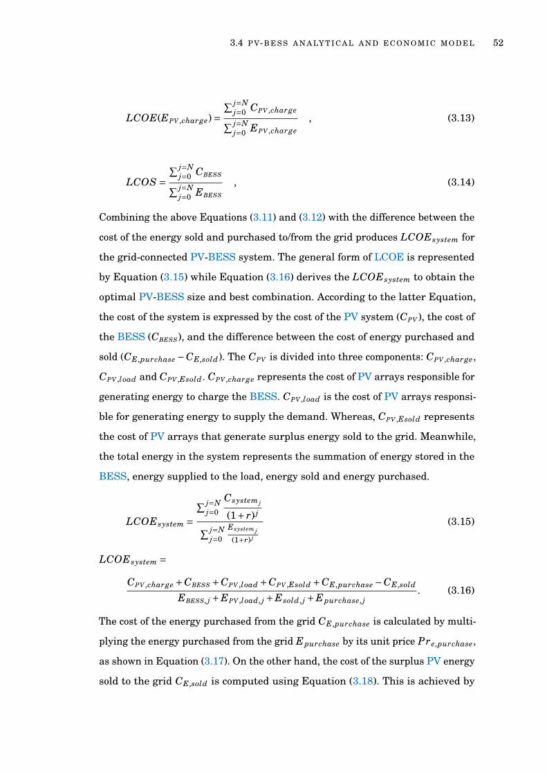
3.4 P V-B E S S A N A LY T I CA L A N D E C O N O M I C M O D E L 52
LCOE(EPV ,charge)=∑ j=N
j=0 CPV ,charge∑ j=Nj=0 EPV ,charge
, (3.13)
LCOS =∑ j=N
j=0 CBESS∑ j=Nj=0 EBESS
, (3.14)
Combining the above Equations (3.11) and (3.12) with the difference between the
cost of the energy sold and purchased to/from the grid produces LCOEsystem for
the grid-connected PV-BESS system. The general form of LCOE is represented
by Equation (3.15) while Equation (3.16) derives the LCOEsystem to obtain the
optimal PV-BESS size and best combination. According to the latter Equation,
the cost of the system is expressed by the cost of the PV system (CPV ), the cost of
the BESS (CBESS), and the difference between the cost of energy purchased and
sold (CE,purchase −CE,sold). The CPV is divided into three components: CPV ,charge,
CPV ,load and CPV ,Esold. CPV ,charge represents the cost of PV arrays responsible for
generating energy to charge the BESS. CPV ,load is the cost of PV arrays responsi-
ble for generating energy to supply the demand. Whereas, CPV ,Esold represents
the cost of PV arrays that generate surplus energy sold to the grid. Meanwhile,
the total energy in the system represents the summation of energy stored in the
BESS, energy supplied to the load, energy sold and energy purchased.
LCOEsystem =∑ j=N
j=0
Csystem j
(1+ r) j∑ j=Nj=0
Esystem j(1+r) j
(3.15)
LCOEsystem =CPV ,charge +CBESS +CPV ,load +CPV ,Esold +CE,purchase −CE,sold
EBESS, j +EPV ,load, j +Esold, j +Epurchase, j. (3.16)
The cost of the energy purchased from the grid CE,purchase is calculated by multi-
plying the energy purchased from the grid Epurchase by its unit price Pre,purchase,
as shown in Equation (3.17). On the other hand, the cost of the surplus PV energy
sold to the grid CE,sold is computed using Equation (3.18). This is achieved by

3.4 P V-B E S S A N A LY T I CA L A N D E C O N O M I C M O D E L 53
multiplying the PV energy sold to the grid Esold by the unit price of energy sold
to the grid Pre,sold. Pre,purchase and Pre,sold are obtained from ScottishPower
Standard Domestic Tariff [149] and given in Table 3.1.
CE,purchase = Epurchase ·Pre,purchase . (3.17)
CE,sold = Esold ·Pre,sold . (3.18)
Equations (3.19)-(3.22) clarify how to find the first four terms in the numerator
of Equation (3.16). The PV-BESS system lifetime N is considered 30 years and
the discount rate r equals 5%. Table 3.1 shows all the parameters values and costs
of the PV that is used for PV cost and energy calculations. Whereas Table 3.2
presents the parameters used for LAB, LIB and RFB cost and energy calculation.
The four terms in the denominator of the LCOEsystem equation are calculated
using the Equations (3.23)-(3.25).
CBESS = ICBESS +j=N∑j=0
CBESS,OM
(1+ r) j . (3.19)
CPV ,charge = (ICPV +j=n∑j=0
CPV ,OM
(1+ r) j ) ·NPV extraT . (3.20)
CPV ,load = (ICPV +j=N∑j=0
CPV ,OM
(1+ r) j ) ·NPV loadT . (3.21)
CPV ,Esold = (ICPV +j=N∑j=0
CPV ,OM
(1+ r) j ) ·NPV EsoldT . (3.22)
EBESS = ηrt
j=N∑j=0
EPV ,Extra · (1−DEGBESS) j
(1+ r) j . (3.23)
EPV ,load, j =j=N∑j=0
EPV ,load · (1−DEGPV ) j
(1+ r) j . (3.24)

3.5 R E S U LT S A N D D I S C U S S I O N 54
Esold, j =j=N∑j=0
Esold · (1−DEGPV ) j
(1+ r) j . (3.25)
The terms NPV loadT , NPV EsoldT , and NPV extraT represent the fractions of PV
arrays that generate energy to supply demand, sell to the grid and to charge the
BESS respectively. These terms are calculated using Equations (3.26)-(3.28).
NPV chargeT =∑i=Y
i=0 PPV ,charge,i
ηPV∑i=Y
i=0 IPV ,i. (3.26)
NPV loadT =∑i=Y
i=0 PPV ,load(n)
ηPV∑i=Y
i=0 IPV (n). (3.27)
NPV EsoldT =∑i=Y
i=0 PPV ,Esold,i
ηPV∑i=Y
i=0 IPV (n), (3.28)
where Y is is the total number of hours in a year (Y=8760 hour), ηPV is the PV
efficiency. Tables 3.1 and 3.2 shows the description and values of all parameters
used in the proposed technical and economic models for the grid-connected PV-
BESS system.
The optimal sizing of the grid-connected PV-BESS system obtained by the
AES is presented in the following section. Moreover, a comparison between the
three combinations; PV-LAB, PV-LIB, and PV-RFB is conducted to evaluate the
performance of these combinations.
3.5 R E S U LT S A N D D I S C U S S I O N
The aim of the proposed approach is to find the optimal size of the combination PV-
BESS for a grid-connected system using AES approach. Three types of batteries
are considered in this research, LAB, LIB, and RFB. The solar radiation and
temperature profiles used in these simulations are for the Isle of Wight and
adopted from National Laboratory of the US Department of Energy (NREL) [2].

3.5 R E S U LT S A N D D I S C U S S I O N 55
Since it was challenging to get the actual demand profiles for the Isle of Wight, the
profiles used in these simulations were obtained from OpenEI (US Department
of Energy) [3].
In this research, the lifetime of the system is 30 years, where the BESSs,
inverter and charge controller are replaced twice during the system lifetime at
10 and 20 years. Using Equation (3.6), the capacities of the BESSs are calculated
for 5 HA. As illustrated in Table 3.2, the variations in capacities were around
1 MWh, and so all of the three types of the BESSs are assumed to have the
capacity of 1 MWh.
The simulations are performed in MATLAB, and the relationship between
various sizes of PV with the three BESS are illustrated in Figure 3.6. Each line
represents the LCOE of the three combinations: PV-LAB, PV-LIB, and PV-RFB.
To determine the optimal PV-BESS combination in terms of minimum cost, the
obtained LCOE values for each combination should be less than the unit price of
the energy purchased from the grid (0.13822 £/kWh). Referring to Figure 3.6, the
minmum LCOE across the three combinations occurs when PPV ,rated = 710 kW
for the combination PV-RFB and LCOEsystem = 0.1135 £/kWh. The minimum
LCOE for the combination PV-LAB happening for PPV ,rated = 590 kW and
LCOEsystem = 0.1167 £/kWh. Whereas the minimum LCOE for the combina-
tion PV-LIB founded at PPV ,rated = 710 kW and LCOEsystem = 0.1348 £/kWh.
These results presented in Table 3.3 besides the value LCOE for the three com-
binations at PPV ,rated = 710 kW. As detailed in Table 3.3, it is observable that
both combinations PV-LIB and PV-RFB have the same PPV ,rated, however, the
LCOEsystem for PV-LIB is higher. That results in selecting the combination PV-
RFB with PPV ,rated = 710 kW as the optimal size for the grid-connected system.
In contrast, the PV rated power for PV-LAB combination is 590 kW but the
LCOEsystem for this combination equals to 0.1167 £/kWh. Since the main objec-
tive for this study is to find the optimal combination of PV and BESS based on
minimum LCOE, the best selection is PV-RFB system with PPV ,rated = 710 kW.
Additionally, Table 3.3 shows the LCOE for the three combinations when PV
rated power is 710 kW . The LCOEsystem is minimum at 710 kW PV rated power

3.5 R E S U LT S A N D D I S C U S S I O N 56
Figure 3.6: The relationship between different values PPV ,rated and LCOE for the threecombinations; PV-LAB, PV-LIB, and PV-RFB.
Table 3.3: Summary of the results obtained from Figure 3.6 regarding the minimumLCOE at PPV ,rated = 710 kW and the value of PV rated power at minimumLCOEsystem for the three PV-BESS systems.
PV-BESSLCOEsystem atPPV ,rated = 710 kW
Min LCOEsystemPPV ,rated atmin LCOEsystem
PV-LAB 0.1211 £/kWh 0.1167 £/kWh 590 kWPV-LIB 0.1348 £/kWh 0.1348 £/kWh 710 kWPV-RFB 0.1135 £/kWh 0.1135 £/kWh 710 kW
Table 3.4: LCOD for the three BESSs; LAB, LIB and RFB when PPV ,rated = 710 kW.
BESS LCOD (£/KWh)
LAB 0.1670
LIB 0.1711
RFB 0.1394
for the combination PV-RFB. The reason behind having minimum LCOE for the
combination PV-RFB can be clarified by referring to Table 3.2 that presents the

3.5 R E S U LT S A N D D I S C U S S I O N 57
Figure 3.7: The relationship between different values PPV ,rated and LCOD for the threeBESSs; LAB, LIB, and RFB.
cost data for the three types of the BESSs. The table shows that the lifetime
for RFB generally ranges between 10-15 years and is chosen to be 10 years in
this study. This implies that the BESS changed twice during the project lifetime
at 10 and 20 years. This equally applied to the other two BESSs. Therefore, to
compare the three BESSs, their costs and degradation rates are considered. The
initial cost ICBESS is less for LAB and higher for LIB, while the operation and
maintenance cost CBESS,OM is higher for LAB and less for LIB. Observing these
data, it is found that the RFB costs are intermediate between LAB and LIB.
Considering that DEGBESS causes a direct effect on finding the energy supplied
by the BESS (Equation (3.23)), this value plays a significant role in determining
the LCOEsystem. The DEGBESS for RFB is the lowest between the three types of
the BESSs which 0.1% compared to 2% and 3.7% for LIB and LAB respectively.
Figure 3.7 shows the LCOD for the three types of the BESSs, LAB, LIB and
RFB. As can be seen from this figure, the RFB has the minimum LCOD compared
to LAB and LIB. Referring to Table 3.4, the values of LCOD for the three types
of the BESSs are presented for PPV ,rated = 710 kW. This also confirms why the

3.5 R E S U LT S A N D D I S C U S S I O N 58
RFB is the best option to be combined with the PV for the grid-connected system.
Furthermore, the LCOD values are higher than LCOE values for the three PV-
BESS combinations. This is due to the high cost of BESS and the energy stored
in it is small compared to the energy produced by the whole system. The ratio
of the BESS cost to its energy is higher than the ratio of the total system cost
to its produced energy. This is the reason why the LCOD values are shown in
Figure 3.7 are higher than the system LCOE values.
Three case studies are selected which are the three PV-BESS combinations pre-
sented in Table 3.3. Each combination has the value of PPV ,rated and LCOEsystem
presented in the table. A comparison is performed between these studies to
evaluate which combination has the optimal size and BESS type.
• Case study 1: PV-LAB system at PPV ,rated = 590 kW and
LCOEsystem = 0.1167 £/kWh.
A comparison between PV-LAB system, the grid-connected PV system
alone, and the case where there is no integration of the PV and BESS are
presented in Table 3.5. The amount of yearly energy production, yearly
energy demand and the energy purchased and sold from/to the grid for
the three scenarios are presented in Table 3.5. The total energy demand
for one year is 1093.4 MWh. For PV-LAB system the percentage of PV
contribution is 83% which is more than the PV contribution for PV alone.
Moreover, the energy purchased from the grid is 656.61 MWh, which
is obviously less than the energy purchased in the other two scenarios.
However, the energy production from the grid-connected PV-LAB system
for one year is 437.79 MWh, this energy is used to supply the demand. The
surplus PV energy sold to the grid is 88.76 MWh. While in case of PV only
system the production is 525.76 MWh, almost half of the generated energy
is directed to the demand. The remaining energy is sold to the grid, and an
amount of 808.91 MWh is purchased from the grid which is higher than
the same value in the PV-LAB scenario.
Figure 3.8 demonstrates the energy purchased and sold for one year. It
is observed that during winter the energy purchased from the grid is

3.5 R E S U LT S A N D D I S C U S S I O N 59
Jan Feb Mar Apr May Jun Jul Aug Sep Oct Nov Dec
Figure 3.8: Energy purchased and extra PV energy sold to the grid for the combinationPV-LAB and PPV ,rated = 590 kW and BatC = 1 MWh.
considerably higher than in summer, this is because of the lower generation
of PV energy in winter. The surplus PV energy sold to the grid is high
in the summer period and is approximately zero during the rest of the
year. Figure 3.9 displays the LAB state of charge during the corresponding
year, the soc during summer days is higher due to the availability of solar
radiation.
Table 3.5: PV-LAB system, PV system only and Grid only scenarios, where PPV ,rated=590kW and LAB BatC=1 MWh
Parameter PV-LAB Grid only PV only
Energy Produced 437.79 MWh 0 MWh 525.76 MWhEnergy Demand 1093.4 MWh 1093.4 MWh 1093.4 MWh
Energy Purchased 655.61 MWh 1093.4 MWh 808.91 MWhEnergy Sold 88.76 MWh 0 MWh 241.22 MWh
PV contribution 83% 0 % 54.1%

3.5 R E S U LT S A N D D I S C U S S I O N 60
Jan Feb Mar Apr May Jun Jul Aug Sep Oct Nov Dec
Figure 3.9: State of charge for lead-acid BESS for one calendar year.
• Case study 2: PV-LIB system at PPV ,rated = 710 kW and
LCOEsystem = 0.1348 £/kWh.
The amount of yearly energy production, yearly energy demand and the
energy purchased and sold from/to the grid are presented in Table 3.6.
The table shows these values for the three scenarios same as case study 1.
Compared to the previous case study, PV-LIB energy production is higher
since the PV rated power is higher. The energy purchased from the grid
for the PV-LIB is less than in case study 1, whereas the energy sold to the
grid is more. However, the LCOE of this system is higher than the previous
case study the highest between all the three case studies as it is seen in
the next case study.
The summary of the comparison between PV-LIB and the other two scenar-
ios in Table 3.6 yields that the integration of LIB is more beneficial than
using PV alone or completely depending on the grid. Figure 3.10 provides

3.5 R E S U LT S A N D D I S C U S S I O N 61
Table 3.6: PV-LIB system, PV system only and Grid only scenarios where PPV ,rated=710kW and LIB BatC=1 MWh
Parameter PV-LIB Grid only PV only
Energy Produced 477.18 MWh 0 MWh 632.69 MWhEnergy Demand 1093.4 MWh 1093.4 MWh 1093.4 MWh
Energy Purchased 616.22 MWh 1093.4 MWh 789.14 MWhEnergy Sold 156.3 MWh 0 MWh 328.38 MWh
PV contribution 75.3% 0 % 48.1%
the distribution of the energy purchased from the grid during winter and
surplus energy sold to the grid during summer. While Figure 3.11 shows
LIB soc for one year of the study.
Jan Feb Mar Apr May Jun Jul Aug Sep Oct Nov Dec
Figure 3.10: Energy purchased and extra PV energy sold to the gridfor the combinationPV-LIB and PPV ,rated = 710 kW and BatC = 1 MWh.
• Case study 3: PV-RFB system at PPV ,rated = 710 kW and
LCOEsystem = 0.1135 £/kWh.

3.5 R E S U LT S A N D D I S C U S S I O N 62
Jan Feb Mar Apr May Jun Jul Aug Sep Oct Nov Dec
Figure 3.11: State of charge for lithium-ion BESS for one calendar year.
In this case study, the results obtained from the simulations are pre-
sented in Table 3.7. Since all the three BESSs in all the case studies
have the same capacity, and the PPV ,rated = 710 kW similar to case study 2,
the results obtained are the same as the previous case study. The ob-
vious difference between this case study and case study 2 is that the
LCOEsystem = 0.1135 £/kWh, indicating a significant reduction in LCOE
compared to the previous study. From the data in Tables 3.5 , 3.6 and 3.7,
Table 3.7: PV-RFB system, PV system only and Grid only scenarios. PPV ,rated=710 kWand RFB BatC=1 MWh
Parameter PV-RFB Grid only PV only
Energy Produced 476.38 MWh 0 MWh 632.69 MWh
Energy Purchased 616.22 MWh 1093.4 MWh 789.14 MWh
Energy Sold 156.3 MWh 0 MWh 328.38 MWh
PV contribution 75.3% 0 % 48.1%
it is obvious that the system PV-RFB has the minimum LCOE across the
three case studies and PV-LIB has the maximum LCOE. Regarding to these

3.5 R E S U LT S A N D D I S C U S S I O N 63
findings, the system PV-RFB is considered the best combination for the
grid-connected PV-BESS for the Isle of Wight. Although the performance of
PV-LIB and PV-RFB are the same, the economic metric plays an important
role in deciding the optimal combination for the grid-connected PV-BESS.
As previously mentioned the performance of the system in case study 3 is
simillar to case study 2, this is indicated in Figures 3.12 and 3.13 that repre-
sent the energy exchanged from/to the grid for PV-RFB and state of charge
for RFB. These figures are also similar to Figure 3.10 and Figure 3.11, but
when refering to Fig 3.6 it is clearly noticed that the PV-RFB is the most
economic option compared to the other systems.
According to the above case studies and the results obtained that the combi-
nation PV-RFB are the optimal combination, Table 3.8 displayes the sizes of te
grid-connected system. The inverter size can be found by Pinv = 1.1 ·PPV .
Jan Feb Mar Apr May Jun Jul Aug Sep Oct Nov Dec
Figure 3.12: Energy purchased and extra PV energy sold to the gridfor the combinationPV-LIB and PPV ,rated = 710 kW and BatC = 1 MWh.

3.6 C O N C L U D I N G R E M A R K S 64
Jan Feb Mar Apr May Jun Jul Aug Sep Oct Nov Dec
Figure 3.13: State of charge for redox flow BESS for one calendar year.
Table 3.8: PV-RFB components sizes.
Component Size
PV 710 kWRFB 1 MWh
Inverter 781 kW
3.6 C O N C L U D I N G R E M A R K S
In this chapter, a technical and economic model for determining the optimal
sizing of a grid-connected PV-BESS system for different battery technologies is
proposed. An improved formula for LCOE is utilised to find the best PV-BESS
combination at the optimal PV rated power. The LCOE calculation includes new
parameters to reflect the impact of surplus PV output and the energy purchased
from the grid, as well as looking at the PV system cost in a different way by
dividing it into three parts: i) the cost of the part generating energy to supply the
load; ii) the cost of the part generating energy to charge the battery; and iii) the

3.6 C O N C L U D I N G R E M A R K S 65
cost of the part generating surplus energy. The obtained results show that the
best type of BESS to be integrated with the PV is RFB. After examining three
combinations of PV-BESS, it is found the minimum system LCOE (0.1135 £/kW)
is for the RFB with a capacity of 1 MWh, and PV size of 710 kW. A reduction
of 18% of electricity cost with respect to the grid electricity price is obtained.
Moreover, the proposed model allows for 75% of the PV contribution of the PV-
RFB system compared to 48% when using the PV alone. After investigating the
AES approach for finding the optimal size for a PV-BESS, the following chapter
employs this approach in an integrated framework. The key objective of the
framework is to find the optimal size-EMS combination for a stand-alone HES.
4
T H E I N T E G R AT E D F R A M E W O R K
4.1 I N T R O D U C T I O N
Chapter 3 showed the AES approach for sizing grid-connected PV-BESS system.
The optimal size and PV-BESS combination are obtained based on minimum
LCOE. An improved formula of LCOE is introduced to determine the optimal
size of the grid-connected microgrid. However, in remote areas, the grid extension
is very costly and the expense of fuel increases drastically. As a result, the
development of stand-alone HESs becomes necessary as an alternative solution
to the grid-connected systems.
In this chapter, the integrated framework for determining the best size-EMS
combination for a HES is introduced. Figure 4.1 illustrates the integrated frame-
work presented in this chapter. Fundamental to this framework is utilising FA to
implement and instantiate multiple EMSs. The proposed integrated framework
consists of three main steps. First, an AES approach is performed to find the
initial sizes of the HES assets based on an initial EMS. Second, using FA to
implement the initial EMS and instantiate different EMSs. Third, an evaluation
model is developed to assess the instantiated EMSs and select the featured con-
ditions to develop an improved EMS. This improved EMS is used to re-exercise
the AES approach to obtain the best size-EMS combination. This chapter further
explores the significance of maximising the use of PV generated energy to reduce
the total LCOE.
66

4.1 I N T R O D U C T I O N 67
An
aly
tica
l M
od
el
Eco
no
mic
Mo
del
O
pti
ma
l si
ze
Op
tim
al
size
/EM
S
com
bin
ati
on
EM
S1
EM
S2
EM
Sk
. . .
Per
form
an
ce i
nd
ices
Per
form
an
ce i
nd
ices
Per
form
an
ce i
nd
ices
Ev
alu
ati
on
Mo
del
. . .
An
aly
tica
l a
nd
Eco
no
mic
Siz
ing
Inst
an
tiati
ng
va
rio
us
EM
Ss
E
va
lua
tion
Mo
del
wit
h f
eed
ba
ck
. . .
EM
Sn
ew
EM
S
Sola
r ra
dia
tion
&
tem
per
atu
reS
pec
ific
ati
on
s &
cost
pa
ram
eter
s
Ho
url
y l
oa
d
pro
file
sO
per
ati
ng
co
nd
itio
n
Op
era
tin
g c
on
dit
ion
Op
era
tin
g c
on
dit
ion
Fig
ure
4.1:
Styl
ized
dem
onst
rati
onof
thre
e-st
eppr
opos
edfr
amew
ork:
(1)a
naly
tica
land
econ
omic
sizi
ng;(
2)us
ing
FAto
gene
rate
vari
ous
EM
S;an
d3)
eval
uati
onm
odel
and
feed
back
.

4.2 H E S S T R U C T U R E A N D M O D E L L I N G I N FI N I T E AU T O M ATA 68
4.2 H E S S T R U C T U R E A N D M O D E L L I N G I N FI N I T E AU T O M ATA
This section introduces the architecture of the HES, a brief background of FA
with an illustration example. Then it describes the implementation of the initial
EMS in FA in detail.
4.2.1 HES Architecture
A simplified scheme of stand-alone HES is reported in Figure 4.2. The HES
consists of PV, BESS, EL, FC, HT, and DSL. The energy generated from the PV
used to supply the demand and the surplus energy is stored in the BESS. Any
further surplus PV energy is directed to the EL to produce hydrogen which is
stored in the HT. The soc of the BESS is checked continuously, there are two
soc predefined levels that determine the operating point of the FC and DSL. The
first level is socFC when the BESS soc reaches this level, the FC starts operating
after checking if there is available H2 in the HT. The second level is socDSL when
soc of the BESS reaches or goes below this level, the DSL starts operating. All
the energy sources use DC/AC power inverters for the connection to a common
AC bus. Although, in reality, the inverter efficiency is not constant, it is assumed
to be constant in this research.
The next section explains what is FA showing an example of how a single asset
in the HES can be implemented in the FA. Following that, the implementation of
EMSinitia in FA is clarified.
4.2.2 Modelling the BESS in Finite Automata
Modelling the HES using FA has many advantages: (i) reducing the complexity
of the HES by dividing it into smaller subsystems, (ii) making the control of
each subsystem simpler, (iii) providing a graphical representation of the system
for better understanding of the HES, (iv) reducing the computation time since

4.2 H E S S T R U C T U R E A N D M O D E L L I N G I N FI N I T E AU T O M ATA 69
PV
Hydrogen
TankFuel Cell
Battery
Electrolyzer
Diesel
Generator
Demand
DC
AC
DC
ACAC
DC
DC
AC
AC Bus
Figure 4.2: The network diagram of a stand-alone HES which consists of PV, BESS, FC,EL, HT, DSL, and multiple inverters.
the state transition for each subsystem is done in parallel, (v) providing more
convenient way to modify the predefined conditions or adding new conditions to
the HES, and (vi) increasing the ability to accommodate new subsystems.
To illustrate how a subsystem in HES can be treated as a DES and modeled in
FA, an example of a BESS is presented in Figure 4.3. The BESS in HES has four
states: charging, discharging, idle and OFF. The circles in the figure represent
the states, while the transitions are the events or the operating conditions. The
state with double circles symbolizes the marked state. This state is the final
state that indicates the completion of the operation of any subsystem. In this
context, the marked state occurs when the system reaches to the final hour in
the year. The states and the events are labelled by numbers; the numbers from
0-9 represent the states and any number from 10 and above are used for events.
The description of the conditions is provided in Table 4.1. The states of the BESS
can be explained as follows:

4.2 H E S S T R U C T U R E A N D M O D E L L I N G I N FI N I T E AU T O M ATA 70
• State 0 represent the OFF state which is the initial state, OFF state indi-
cates that BESS is either full (reaches socmax) or empty (reaches socmin).
The BESS is OFF because it is fully charged when the condition 11 is
satisfied "soc ≥ socmax". While the BESS is OFF because it is empty when
condition 13 is satisfied "soc ≤ socmin". From state 0, the BESS can move
either to state 1 or 2 depending on the occurred condition 10 or 12.
• State 1 denotes that BESS is in charging state which the desired state (the
state that the system is preferred to in). The condition related to entering
this state is 10, "Pinput(n) ≥ Pload(n) & soc(n) < socmax". While condition
11 returns the BESS to state 0.
• State 2 is the discharging state, condition 12
"Pinput(n) < Pload(n) & soc(n) > socDSL" is responsible to trans-
fer the BESS from the states 0, 1, and 3 to state 2. Condition 13
"soc ≤ socmin" changes the state of BESS from state 2 to state 0.
• State 3 represents the idle state, where the Pinput(n) at that instance equals
to the demand, leading to entering the BESS in idle state (no charging or
discharging). Conditions 14 or 19, which are responsible to operate the DSL
or FC, move the BESS to state 3. There is no condition that transfers BESS
from state 3 to 0 directly, since the BESS can not move from the idle state
1
0
3
2
Initial state
OFF
(Full/Empty)
State 1
ChargingState 3
Idle
State 2
Discharging
10
10
10
12
12
11
13
14 OR 19
Figure 4.3: Modelling BESS in finite au-tomata.
Table 4.1: Conditions for BESS operation.Conditions Subsystem states Description
10 BESS chargingPinput(n) ≥ Pload(n)& soc(n) < socmax
11 BESS OFF soc(n) ≥ socmax
12 BESS dischargingPinput(n) < Pload(n)& soc(n) > socDSL
13 BESS OFF soc(n) ≤ socmin
14 DSL ONPinput(n)< Pload(n)& soc(n)≤ socDSL
& BFC(n)= 0
19 FC ONPinput(n)< Pload(n)
& soc(n)≤ socFC
& socHT(n)> socHTmin

4.2 H E S S T R U C T U R E A N D M O D E L L I N G I N FI N I T E AU T O M ATA 71
to OFF state without passing the charging or discharging state. Condition
12 transfers BESS from state 3 to 2 and condition 10 makes the BESS move
from states 3 or 2 to 1.
The behavior of any system modeled using FA is usually described by a regular
language and can be found in [153, 154, 155].
4.2.3 Implementing EMS using Finite Automata
The EMS is a group of steps the system follows to manage the energy generated
by all the assets in the HES. The objective of EMS is to guarantee the energy
balance under system constraints and constantly supply the demand. Since the
HES consists of multiple subsystems, a number of states can be assigned to each
subsystem, combining all these states form the total states of the EMS. Thus, the
HES switches between these states according to predefined operating conditions.
This section describes how the EMSinitial used in the initial sizing of the HES is
implemented in FA.
In the previous section, the four states of BESS have been described. In this
section, the states of the rest of the assets in the HES are explained. Each of the
DSL, FC and EL has two states ON and OFF. The HT has three state: OFF (full or
empty), charge and discharge. The state of the PV and the demand are considered
always ON even if the solar radiation is zero or there is no demand. Every state
of the HES combines the sub-states of subsystems and identifies the status of the
HES at each instant in the year. Figure 4.4 shows all the possible states that the
HES can endure. The HES has nine states and each state contains the sub-states
of all assets in the HES. Additionally, each state of the HES identifies the status
of HES at each instant in the year. Meaning which asset is ON/OFF and whether
the BESS and HT are charging or discharging.
TTable 4.2 and Figures 4.4 and 4.5 provide a complete description of the
EMSinitial . Table 4.2 introduces the operating condition that determines the
following state of the HES. Such that the occurrence of one of the operating
conditions in the table decides the state of the HES in the next hour. Figure 4.4

4.2 H E S S T R U C T U R E A N D M O D E L L I N G I N FI N I T E AU T O M ATA 72
State 0
PV: ON
demand: ON
BESS: discharge
DSL: OFF
EL: OFF
FC: OFF
HT: OFF (empty)
State 1
PV: ON
demand: ON
BESS: idle
DSL: ON
EL: OFF
FC: OFF
HT: OFF (empty)
State 2
PV: ON
demand: ON
BESS: charge
DSL: OFF
EL: ON
FC: OFF
HT: charge
State 3
PV: ON
demand: ON
BESS: OFF (empty)
DSL: ON
EL: OFF
FC: OFF
HT: OFF (empty)
State 4
PV: ON
demand: ON
BESS: idle
DSL: OFF
EL: OFF
FC: ON
HT: discharge
State 5
PV: ON
demand: ON
BESS: OFF (full)
DSL: OFF
EL: ON
FC: OFF
HT: charge
State 6
PV: ON
demand: ON
BESS: charge
DSL: OFF
EL: OFF
FC: OFF
HT: OFF (full)
State 7
PV: ON
demand: ON
BESS: discharge
DSL: OFF
EL: OFF
FC: OFF
HT: OFF (full)
State 8
PV: ON
Load: ON
BESS: charge
DSL: OFF
EL: OFF
FC: OFF
HT: OFF (empty)
Figure 4.4: Nine states describing EMSinitial based on finite automata. Each state illus-trates which asset is operating and whether the BESS and HT are chargingor discharging. The PV and demand are considered always as ON state
Figure 4.5: Finite automata model for EMSinitial .

4.2 H E S S T R U C T U R E A N D M O D E L L I N G I N FI N I T E AU T O M ATA 73
Table 4.2: Conditions for EMSinitial .
Conditions Subsystem states Description
10 BESS chargingPinput(n) ≥ Pload(n)& soc(n) < socmax
11 BESS OFF soc(n) ≥ socmax
12 BESS dischargingPinput(n) < Pload(n)& soc(n) > socDSL
13 BESS OFF soc(n) ≤ socmin
14 DSL ONPinput(n)< Pload(n)& soc(n)≤ socDSL
& BFC = 0
15 DSL OFF Pinput(n) > Pload(n)
16 EL ONPEL,min ≤ PPV ,surplus(n)≤ PEL,rated
& socHT(n)< socHTmax
17 EL OFF PPV ,surplus(n) < PEL,min
18 EL OFF socHT(n) ≥ socHTmax
19 FC ONPinput(n)< Pload(n)
& soc(n)≤ socFC
& socHT(n)> socHTmin
20 FC OFF socHT(n) ≤ socHTmin
describes the nine states of the HES. While Figure 4.5 presents the graphical
representation of EMSinitial using FA. EMSinitial has nine states which are all
the possible states that the HES can experience. State 0 is the initial state and
state 2 represent the marked state. The marked state can be defined as the state
at which the HES achieves the desired behavior at the end of the year. In the
first hour of the year, all the subsystems are OFF (the BESS is assumed to be
fully charged at the beginning). During each hour, the power generated from
the PV, DSL, and FC is calculated to find the hourly input power to the BESS
(Pinput). The soc of the BESS and socHT of the HT are computed hourly as well.
All these values are used to find the binary values of DSL, FC, and EL (described
in Section 4.3). These binary values identify the state of each asset in the HES.
EMSinitial starts with state 0, where all the assets are OFF, the BESS in the

4.2 H E S S T R U C T U R E A N D M O D E L L I N G I N FI N I T E AU T O M ATA 74
discharging mode, and the PV is ON. The rest of the states and events can be
explained as follows:
1. From state 0, the HES can move to one of the following states 1, 2, 3 or 8
through the following conditions:
a) Condition 14 leads a movement to state 1, where the DSL is ON, the
BESS is idle and the assets EL, FC, and HT are OFF.
b) Condition 16 moves the HES from state 0 to state 2. This condition
relates to EL operation to generate H2 and consequently the HT is in
charging state. While the BESS is fully charged (i.e. OFF), the FC and
DSL are OFF.
c) Condition 13 moves the HES from state 0 to state 3, in state 3 the
DSL is ON, the BESS is empty (i.e. OFF). The EL, FC, and HT are
OFF.
d) Condition 10 transfers the HES from state 0 to state 8, where there
are surplus power from the PV to charge the BESS. The EL, FC, and
HT are OFF.
e) Condition 12 keeps the HES in state 0.
2. In state 1, the BESS is idle since the DSL is ON. The EL, FC, and HT are
OFF. From state 1, there aretwo destinations the HES can move to, either
state 2 or state 8 and the conditions responsible fo the movemonet are:
a) Condition 16 moves the HES from state 1 to state 2, that relates to
EL operation (see point 1.b).
b) Condition 15 moves the HES from state 1 to state 8. In state 8, the
DSL becomes OFF, since there is surplus power to charge the BESS.
The EL, FC, and HT are OFF.
c) Condition 10 keeps the HES in state 1.
3. In state 2, the BESS is charging and the surplus power is used to operate
the EL. The HT is charging to store H2. The DSL and FC are OFF. From

4.2 H E S S T R U C T U R E A N D M O D E L L I N G I N FI N I T E AU T O M ATA 75
state 2, the HES can move to state 5 or 6 depending on the operating
conditions:
a) Condition 11 moves the HES from state 2 to state 5, the BESS is fully
charged, the EL is still ON and the HT is charging. The DSL and FC
are OFF.
b) Condition 18 transfers the HES from state 2 to state 6, where in this
state the HT is fully charged (i.e. OFF) and the EL is OFF. The DSL
and FC are OFF, while the BESS is charging.
c) The occurrence of condition 16 causes the HES to stay in state 2.
4. In state 3, the BESS is empty and therefore, the DSL is ON. The EL, FC
and HT are OFF. After state 3, the state of HES can be either 2 or 8. The
following conditions can determine the HES destination:
a) Condition 16 moves the HES to state 2 (see point 1.b).
b) Condition 15 transfers the HES to state 8 (see point 2.b).
c) The occurrence of condition 13 causes the HES to stay in state 3.
5. In state 4, the FC is ON and the HT is discharging. When FC is ON this
means the BESS is idle, while the DSL and EL are OFF. From state 4. the
HES has four choices for states 0, 1, 2 or 8 depending on the following
conditions:
a) Condition 20 causes the HES to move to state 0. The FC, HT, and DSL
are OFF. The soc of the BESS is enough to supply the demand so the
BESS is discharging.
b) Condition 14 moves the HES to state 1 (see point 1.a).
c) Condition 16 leads the HES to move to state 2 (see point 1.b).
d) Condition 15 causes the HES to move to state 8 (see point 2.b).
e) Condition 19 Keeps the HES in state 4.

4.2 H E S S T R U C T U R E A N D M O D E L L I N G I N FI N I T E AU T O M ATA 76
6. In state 5, the BESS is fully charged, the surplus power directed to the EL
and the HT is charging. The DSL and EL are OFF. The only option for the
next state is state 7 and happens when condition 18 is satisfied:
a) Condition 18 moves the HES to state 7 (see point 3.b).
b) Condition 16 Keeps the HES in state 5.
7. In state 6, there is surplus power generated by the PV to charge the BESS,
the HT is fully charged. The EL, FC, and the DSL are OFF. From state 6,
the HES can move to state 7 through the following condition:
a) Condition 12 causes the HES to move to state 7, there is no surplus
PV power so the BESS discharges to supply the demand. The DSL,
FC, EL, and HT are OFF.
b) Condition 10 keeps the HES in state 6.
8. In state 7, there is no surplus PV power to supply the demand or charge
the BESS, so the demand is supplied by the BESS. The DSL, FC, and EL
are OFF and HT are fully charged. The next state of the HES is state 4 and
can be achieved through the following condition:
a) Condition 19 moves the HES to state 4, the soc of the BESS reaches
to a level where it is required to operate the FC. The HT discharges to
supply the FC with H2, whereas the EL and DSL are OFF. The BESS
is in idle mode.
b) Condition 12 Keeps the HES in state 7.
9. In state 8, the BESS is charging, while the HT is empty. The EL, FC, and
the DSL are OFF. The next state of the HES is state 2 and can be achieved
through condition 16:
a) Condition 16 leads the HES to move to state 0 (see point 1.b).
b) Condition 10 keeps the HES in state 8.
To this end, all the states and conditions of EMSinitial are explained and the rela-
tionship between conditions and states are clarified. Depending on this FA model

4.3 A N A LY T I CA L M O D E L L I N G O F H E S 77
of EMSinitial , three different EMSs are instantiated. The process is explained in
Section 4.6.1.
The following section demonstrates the analytical and economic approach AES.
The AES is the initial step in the integrated framework that utilises EMSinitial
to find the initial size of the HES assets.
4.3 A N A LY T I CA L M O D E L L I N G O F H E S
The AES performed in this chapter follows the same calculation steps as in
Chapter 3. The AES in Chapter 3 is developed for a grid-connected PV-BESS
microgrid. Whereas the AES utilised in this chapter is for stand-alone HES
composing of multiple assets. Accordingly, the AES approach presented in the
previous chapter needs to be modified.
The AES approach is used to determine the size of the PV and BESS by
iteratively changing the PV rated power from (0 - α ·Pload,max) kW with a step of
10 kW each time. α is a constant equal to 10 and chosen to ensure the selected
range covers all possible PV sizes. Pload,max in this chapter is 26.7 kW [5] see
Figure 4.9), and therefore, the range of PV rated power is selected (0 - 267) kW.
A factor that determines the BESS size is the Hours of Autonomy (HA), which
means for how many hours a completely charged BESS is able to supply the
demand continuously. Since the HES in this study is stand-alone, it is essential
to select a high value for HA to ensure demand satisfaction. Thereby, HA is
iteratively considered as 12, 24, 36, 48, and 60 hours. The size of the FC and DSL
depend mainly on Pload,max with some factor and this explained in the following
sections. The size of the EL and HT are considered constant.
The EMS utilised by AES approach is the EMSinitial explained in Section 4.2.3.
This EMS guarantees the demand is continuously supplied with energy and at
the same time ensures the other assets of the HES operate efficiently. The main
idea is to generate multiple scenarios with different PV sizes and BESS capacities.
Following that, the LCOE is calculated for each scenario. The combination that
provides the lowest LCOE while covering the demand is selected as the optimal

4.3 A N A LY T I CA L M O D E L L I N G O F H E S 78
solution. To ensure demand satisfaction, a power balance is conducted every time
interval. As such, the total power generated by the PV, DSL, FC, BESS are equal
to the demand and EL. This is represented by Equation (4.1).
Pload(n)+PEL(n)= PPV (n)+PFC(n)+PDSL(n)+PBESS(n) , (4.1)
where Pload(n) and PEL the power needed by the demand and the power consumed
by the EL. PPV (n), PFC(n), PDSL(n) are the hourly power generated by PV, FC
and DSL, respectively. PBESS is the power supplied by the BESS.
The flowchart in Figure 4.6 summarizes the management rules for the AES.
PPV−min and PPV−max are the minimum and maximum values in PV rated power
range. soc is the state of charge of the BESS, and k indicates the number of HA
involved. BFC, BDSL, BEL are binary logic values for the FC, DSL and EL. These
binary values are computed hourly to identify which device is operating at that
time.
The analytical model used for PV in this chapter is the same as the model
explained in details in Chapter 3 (see Section 3.4.1). Newcastle upon Tyne is
considered as a case study to validate this approach. The solar radiation and
temperature data for the city of Newcastle upon Tyne [4] are used to find the
optimal size-EMS of the HES. The demand profile are for 40 houses of the
Customer-Led Network Revolution project [5]. Figures 4.7 and 4.8 illustrate the
profiles of the solar radiation and temperature. Whereas, the data used for PV
analytical model is presented in Table 4.3. The demand profile considered in this
chapter is presented in Figure 4.9. The analytical model for BESS is the same
concept as in Section 3.4.2 with a difference in the input and output power to the
BESS, so it is explained in the next section. Furthermore, the analytical models
for DSL, FC, EL, and HT are demonstrated in Sections 4.3.2 to 4.3.5.
4.3.1 Battery Energy Storage System
The values of the power generated from the PV and the demand power at each
time step, determine whether to charge or discharge the BESS. In the case that

4.3 A N A LY T I CA L M O D E L L I N G O F H E S 79
Start
Compute hourly Ppv ,
PEL, PFC, PDSL, Pinput
using binary logics BEL,
BFC, BDSL
Ppv=Ppv-min
Data input:
Solar radiation,
ttemperature, demand,
specifications.
Compute battery
capacity using HA
n=1
Pinput(n)>Pload(n)
Charge BESS
& supply load
PPV,surplus (n)≥ PEL,min
& PPV,surplus (n)≤ PEL,max
n = 8760
No
n=n+1
Calculate the LCOE for
PV/BESS/DSL
Yes
k=5
Ppv=Ppv-max
Yes
k=k+1
No
No
Ppv=Ppv+step
End
BDSL(n)=0,
BFC(n)=0,
BEL(n)=1
BDSL(n)=1,
BFC(n)=0,
BEL(n)=0
soc(n)<socmax
Yes
Yes
BDSL(n)=0,
BFC(n)=1,
BEL(n)=0
Switch off BESS
No
socHT(n)>socHTmin
soc(n)≤ socFCYes
soc(n)≤socDSLYes
No
No
No
socHT(n)<socHTmax
Yes
Yes
No
Yes
soc(n)>socmin
Discharge BESS
& supply loadSwitch off BESS
No
Yes
No
BDSL(n)=0,
BFC(n)=0,
BEL(n)=0
No
Yes
YesNo BFC(n)=0
Figure 4.6: The flowchart of AES approach showing the steps of the EMS to find theinitial size of the HES.
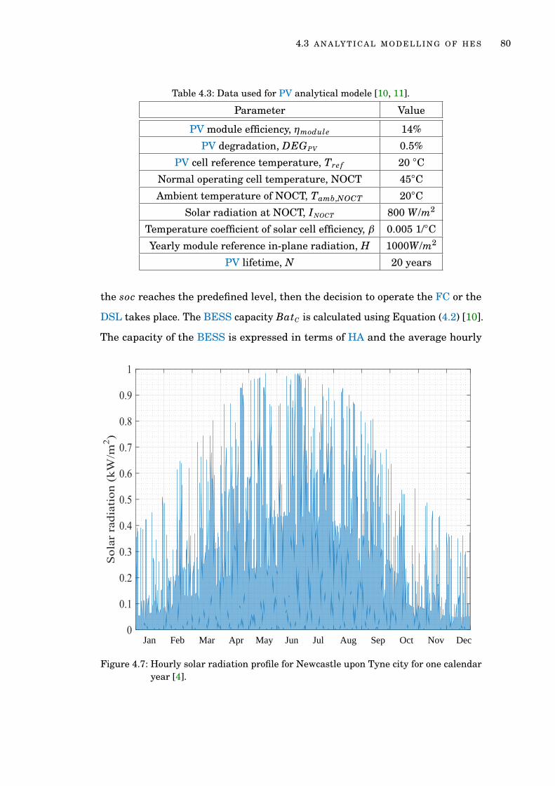
4.3 A N A LY T I CA L M O D E L L I N G O F H E S 80
Table 4.3: Data used for PV analytical modele [10, 11].
Parameter Value
PV module efficiency, ηmodule 14%
PV degradation, DEGPV 0.5%
PV cell reference temperature, Tre f 20 ◦CNormal operating cell temperature, NOCT 45◦CAmbient temperature of NOCT, Tamb,NOCT 20◦C
Solar radiation at NOCT, INOCT 800 W /m2
Temperature coefficient of solar cell efficiency, β 0.005 1/◦CYearly module reference in-plane radiation, H 1000W /m2
PV lifetime, N 20 years
the soc reaches the predefined level, then the decision to operate the FC or the
DSL takes place. The BESS capacity BatC is calculated using Equation (4.2) [10].
The capacity of the BESS is expressed in terms of HA and the average hourly
Jan Feb Mar Apr May Jun Jul Aug Sep Oct Nov Dec
Figure 4.7: Hourly solar radiation profile for Newcastle upon Tyne city for one calendaryear [4].

4.3 A N A LY T I CA L M O D E L L I N G O F H E S 81
Jan Feb Mar Apr May Jun Jul Aug Sep Oct Nov Dec
Figure 4.8: Hourly ambient temperature profile for Newcastle upon Tyne city for onecalendar year [4].
demand Pload,avg. Pload,avg is equal to 10.7 kW, whereas HA ranges between five
values, 12, 24, 36, 48, 60 hours.
BatC = HA ·Pload,avg
ηinv ·ηch ·DOD, (4.2)
where ηinv and ηch are the inverter and BESS charge efficiencies, and DOD
represent the depth of discharge. A fundamental parameter to represent the
available capacity in the BESS is the state of charge (soc), which is used to decide
whether to charge or discharge the BESS. Depending on the power generated by
the HES assets and the demand requirements, the hourly BESS soc for charging

4.3 A N A LY T I CA L M O D E L L I N G O F H E S 82
Jan Feb Mar Apr May Jun Jul Aug Sep Oct Nov Dec
Figure 4.9: Hourly demand profile for Newcastle upon Tyne citry for one calendaryear [5].
and discharging states can be calculated using Equation (4.3).
soc(n)=
soc(n−1)+ [Pinput(n)−Pload(n)] ·ηch ·∆tηinv · BatC
, Pinput(n)> Pload(n) ,
soc(n−1)− [Pload(n)−Pinput(n)] ·∆tηinv ·ηdch ·BatC
, Pinput(n)≤ Pload(n),
(4.3)
where soc(n) and soc(n−1) represent the states of charge of the BESS at n and
n−1, respectively. ηdch is the discharging efficiency and ∆t is the time step. In
this thesis, the value of ∆t is considered to be equal one hour. Pinput(n) is the
sum of input power to the BESS at a specific hour and found using Equation (4.4).
If BESS input power is greater than demand, Pinput(n) > Pload(n), then the
demand is supplied firstly and the surplus poweris used to charge the BESS. On

4.3 A N A LY T I CA L M O D E L L I N G O F H E S 83
the other hand, if Pinput(n) ≤ Pload(n), the power generated is used to supply the
demand and any deficiency is covered by the BESS.
Pinput(n)= PPV (n)+PDSL(n)+PFC(n) . (4.4)
To protect the BESS from overcharging or under-discharging, the BESS soc
should be maintained at a reasonable level. The soc should be maintained be-
tween two limit levels, socmax and socmin subject to the following constraint:
socmin ≤ soc(n)≤ socmax (4.5)
The parameters used in the BESS analytical model are presented in Table. 4.4.
Table 4.4: Data used for battery energy system modelling [10].
Parameter Value
Depth of discharge, DOD 80%
Charge efficiency, ηch 80%
Discharge efficiency, ηdch 80%
Minimum state of charge, socmin 20%
Maximum state of charge, socmax 90%
Round trip efficiency, RTe f f 90%
Degradation rate of battery, DEGBESS 0.1%
Hours of autonomy, HA 12, 24, 36, 48, 60 hrs
4.3.2 Diesel Generator
The power generated from RER is variable and therefore, to ensure the demand
is constantly supplied, the existence of the DSL is necessary. When the integrated
RERs/AER and BESS are unable to supply the demand, the DSL operated to
supply the demand. Any surplus power generated by the DSL is used to charge
the BESS. Since the first priority is to ensure the satisfaction of demand, the

4.3 A N A LY T I CA L M O D E L L I N G O F H E S 84
rated power of the DSL depends on Pload,max (see Figure 4.9) and expressed by
the following equation:
PDSL,rated = MDSL ·Pload,max , (4.6)
where MDSL is the DSL margin coefficient. In this thesis, MDSL is considered to be
1.2 for safety purposes. According to this equation, PDSL,rated=32 kW. The hourly
output of DSL is found using Equation (4.7), and subjected to the constraint in
Equation (4.8):
PDSL(n)=
BDSL(n) ·Pload(n), BDSL(n)= 1 ,
0, BDSL(n)= 0 ,
(4.7)
0≤ PDSL(n)≤ PDSL,rated , (4.8)
where BDSL(n) represents a binary variable that describes the state of the DSL
at a specific hour in the year [156, 157]. The key objective for using BDSL is to
decide whether to activate the DSL or not based on the soc level. Condition 14 in
Table 4.2 describes the operating condition for DSL operation.
4.3.3 Fuel Cell
The FC is used as a backup power generator. The FC is activated when the solar
power is insufficient to supply the demand and soc reaches socFC. Any surplus
in the power generated by the FC is used to charge the BESS. The size of the FC
is determined using the following equation:
PFC,rated = MFC ·Pload,max , (4.9)
where the FC margin coefficient MFC and equals to 1.2 to leave some safe mar-
gin [158]. According to this equation, PFC,rated= 32 kW . The hourly output power

4.3 A N A LY T I CA L M O D E L L I N G O F H E S 85
generated from the FC can be identified by Equation (4.10) and its constraint in
Equation (4.11):
PFC(n)=
BFC(n) ·Pload(n), BFC(n)= 1 ,
0, BFC(n)= 0 ,
(4.10)
0≤ PFC(n)≤ PFC,rated , (4.11)
where BFC(n) is a binary variable that describes the state of the FC at any hour
in the year [156, 157]. Condition 19 in Table 4.2 shows the operationg condition
for FC operation. The input hydrogen to the FC is consumed from the hydrogen
tank. The FC consumption of hydrogen for 1 kW rated power in one hour can be
calculated by [29]:
H2,cons,1kW = 1kW2 ·VFC ·F
·3600
= 10002 ·0.7 ·96487
·3600= 26.8 mol/h ,(4.12)
where H2,cons,1kW represent the amount of hydrogen consumed by the FC at 1 kW
which depends on the FC voltage VFC, and Faraday constant F (see Table 4.5).
The hourly amount of hydrogen consumed by the FC H2,cons(n) can be determined
by multiplying the value of H2,cons,1kW by PFC(n). Equation (4.13) illustrates the
hourly H2 consumed by the FC.
H2,cons(n)=
PFC(n) ·H2,cons,1kW , PFC(n)> 0 .
0, PFC(n)≤ 0 .
(4.13)
4.3.4 Electrolyser
The purpose of using the EL is to produce hydrogen through the electrolysis
of water. The produced hydrogen is stored in the HT and used as needed to
operate the FC. The output pressure of hydrogen is considered 20 bar [159] in

4.3 A N A LY T I CA L M O D E L L I N G O F H E S 86
this thesis. The hourly input power to the EL and its constraints can be identified
by Equations (4.14) and (4.15):
PEL(n)=
BEL(n) ·PPV ,surplus(n), BEL(n)= 1 ,
0, BEL(n)= 0 ,
(4.14)
PEL,min ≤ PEL(n)≤ PEL,rated , (4.15)
where PEL,min = 20% ·PEL,rated. While BEL(n) represents a binary variable that
describes the state of the EL at any hour in the year [156, 157]. The value of
BEL(n) decides whether to operate the EL or not. Condition 16 in Table 4.2 defines
the EL operation. If the value of PPV ,surplus(n) is sufficient to operate the EL and
the state of charge of HT is less than the maximum, BEL(n) is set to one and
the EL generates hydrogen. To operate the EL, the value of the working voltage
between its electrodes Vel needs to be 2 volts [29]. According to Faraday’s law,
the amount of hydrogen produced by the EL for 1 kW rated power in one hour,
H2,prod,1kW , can be calculated by [29]:
H2,prod,1kW = 1kW2 ·Vel ·F
·3600
= 10002 ·2 ·96487
·3600= 9.33 mol/h .(4.16)
All the values used in calculations can be found in Table 4.5. The hourly amount
of hydrogen produced by the EL, H2,prod(n) is determined by multiplying the
value of H2,prod,1kW by PEL(n). This is illustrated in following equation:
H2,prod(n)=
PEL(n) ·H2,prod,1KW , PEL(n)> 0 .
0, PEL(n)≤ 0 .
(4.17)
PEL,rated is chosen to be 100 kW in this study. The reason for this is to guarantee
that all the surplus power generated by the PV is utilised by the EL to generate
hydrogen. Any surplus PV power between 20% and 100% of the PEL,rated is used
to generate H2.

4.3 A N A LY T I CA L M O D E L L I N G O F H E S 87
4.3.5 Hydrogen Tank
The HT is required to store the hydrogen produced from the EL for later use by
the FC. The HT analytical model assumes during the process of adding hydrogen
to the tank, no energy is used and the tank experiences no leakage. The hydrogen
produced by the EL provides another option for storing the surplus PV power.
The size of the HT SHT in kgs is determined by Equation (4.18), where the HT
capacity depends strongly on the H2 produced by the EL. EHT is the tank size in
kWh and given by Equation (4.19) [160]:
SHT = HAHT2 ·H2,prod,1kW ·Prated,EL ·H2mass , (4.18)
EHT = HAHT2 ·H2,prod,1kW ·PEL,rated ·H2mass ·LHV , (4.19)
HAHT2 represents the hours of autonomy for the HT and considered 48 hours in
this thesis. H2mass is the molar mass of hydrogen gas, and LHV is hydrogen
low heating value and presented in Table 4.5. According to Equations (4.18)
and (4.19), the size of HT is 89.5 kg and 2955 kWh.
The level of hydrogen in the tank increases if the EL is operating, however, it
decreases when the FC is generating power. Equation (4.20) determines the
hourly state of charge of the HT socHT(n) in both cases.
socHT(n)=
socHT(n−1)+ H2,prod(n) ·H2mass ·LHV ·∆tEHT
, PEL(n)> 0,
socHT(n−1)− H2,cons(n) ·H2mass ·LHV ·∆tEHT
, PFC(n)> 0,
(4.20)
where socHT(n−1) is the hydrogen level in the tank at time n−1. At any time
the socHT(n) is subjected to the following constraint:
socHTmin ≤ socHT(n)≤ socHTmax (4.21)
Table 4.5 presents all the values that is needed by the analytical models of the
FC, EL, and HT.

4.4 T H E E C O N O M I C M O D E L L I N G 88
Table 4.5: Data used for hydrogen system modelling (FC, EL, and HT).
Parameter Value Ref.
socHTmin 10% -
socHTmax 90% -
Pressure, PFC 20 bar [159]
Faraday constant, F 96487 C/mol [29]
FC voltage, VFC 0.7 volts [29]
EL voltage, Vel 2 volts [29]
H2 low heating value, LHV 33 kWh/kg [29]
Mole mass of H2 gas, H2mass 0.002 kg/mol [29]
FC margin coefficient, MFC 1.2 [158]
HT hours of autonomy, HAH2 48 hrs -
4.4 T H E E C O N O M I C M O D E L L I N G
The LCOE methods are widely used to evaluate the economic feasibility of RERs.
The costs distributed over the project lifetime are considered, and this provides
a more accurate economic picture of the project under analysis [10]. In general,
the LCOE is the total system cost computed across the lifetime of the system
divided by the energy generated from that system also across the lifetime. It is
noted here the FC, EL, and HT are not included in the calculation of the LCOE
since this increases the complexity of the system. Equation (4.22) represents the
general form of the LCOE.
LCOE = Total S ystem CostsTotal Energy Production
(£/kWh)
=N∑
j=0
Costsystem
(1+ r) j
Esystem
(1+ r) j
,
(4.22)
where the total system cost Costsystem represents the sum of the total costs of
the PV, BESS, DSL and the inverters and presented by the following equation:
Costsystem = CPV +CBESS +CDSL +CInv , (4.23)

4.4 T H E E C O N O M I C M O D E L L I N G 89
where CPV is the total cost of PV, CBESS is the total cost of BESS, CDSL is the total
cost of the DSL, and CInv is the cost of the inverters for the PV and BESS. The
total cost of any asset in the HES, Csystem is presented in Equation (4.24).
Csystem = ICsystem +OMsystem +RCsystem . (4.24)
where ICsystem represents the initial cost of all the assets in the HES. The
OMsystem is the operation and maintenance cost of all the assets and RCsystem is
the replacement costs of the assets that need to be replaced. All these costs are
described in detail in the following sections. The denominator of Equation 4.22
is the Esystem and represents the total energy generated by the PV/BESS/DSL.
Equation 4.25 shows how to find Esystem.
Esystem = EPV ,T +EBESS,T +EDSL,T , (4.25)
4.4.1 Photovoltaic
The total cost of the PV is the sum of the initial costs, maintenance costs, and
replacement costs. The lifetime for PV is 20 years which the same as the HES
lifetime, so there are no replacement costs. Equation (4.26) illustrates the total
costs for PV.
CPV = ICPV +∑ j=N
j=0 CPV ,OM
(1+ r) j , (4.26)
where N is the HES lifetime and equals to 20 years, r is the discount rate and
considered to be 5% in this thesis. The total energy generated from the PV
discounted during its lifetime EPV ,T, can be found using the following equation:
EPV ,T =j=N∑j=0
∑n=8760n=0 EPV · (1−DEGPV ) j
(1+ r) j , (4.27)
DEGPV is the degradation rate of the PV and equals to 0.5%. All the costs related
to PV can be found in Table 4.7.

4.4 T H E E C O N O M I C M O D E L L I N G 90
4.4.2 Battery Energy Storage System
The BESS is replaced once during the HES lifetime. The replacement cost of the
BESS is equal to the initial cost. The total cost of the BESS is calculated using
the following equation:
CBESS = ICBESS +∑ j=N
j=0 CBESS,OM
(1+ r) j +∑
j=10 RCBESS
(1+ r) j , (4.28)
The energy produced by the BESS can be found using Equation (4.29).
EBESS,T = ηrt ·j=N∑j=0
∑n=8760n=0 EPV ,charge · (1−DEGBESS) j
(1+ r) j , (4.29)
where EPV ,charge is the PV energy used to charge the BESS. ηrt is the round trip
efficiency for the BESS and DEGBESS is the degradation rate for the BESS.
4.4.3 Diesel Generator
The total cost of DSL include the following four parts: (i) the initial cost of the DSL
(ICDSL), (ii) the operating and maintenance cost (OMDSL), (iii) the replacement
cost (RCDSL), and (iv) the cost of the fuel consumed by the DSL (CDSL, f uel).
The total fuel can be calculated by Equation (4.30) and the total cost of the fuel
found by Equation (4.31).
Fconsume(n)=
A·PDSL,rated+B·PDSL(n), PDSL(n) > 0.
0, PDSL(n) = 0.
(4.30)
CDSL, f uel(n)=
Fconsume(n) · fp, Fconsume(n)> 0.
0, Fconsume(n)= 0.
(4.31)
where A and B are DSL consumption curve coefficients (Liter/kWh), fp is the
DSL fuel unit cost (£/Liter).

4.4 T H E E C O N O M I C M O D E L L I N G 91
The DSL lifetime is given in hours, Li f eDSL,h, and can be found in years using
Equation (4.32). Li f eDSL,y is essential to calculate the replacement cost for the
DSL.
Li f eDSL,y =Li f eDSL,h
WHDSL. (4.32)
The total cost of the DSL can be found using the following equation:
CDSL =ICDSL +∑ j=N
j=0 CDSL,OM
(1+ r) j +∑j=Li f eDSL,y RCDSL
(1+ r) j +∑ j=N
j=0 CDSL, f uel
(1+ r) j ,
(4.33)
and the total energy generated by the DSL is calculated using Equation (4.34).
EDSL,T =j=N∑j=0
∑n=8760n=0 EDSL
(1+ r) j . (4.34)
Tables 4.6 presents the costs for the PV, DSL, inverters, and BESS. The costs in
the table are divided into initial, operating and maintenance, and replacement
costs. Table 4.7 shows the data required for the economic models for the above-
mentioned assets.
Table 4.6: The cost and lifetime of the HES assets [10, 12].
Component IC Yearly OM RC Lifetime
PV 2508 £/kW 33 £/kW 0 20 years
DSL 374 £/kW 0.1 £/kW 356 £/kW 15,000 hrs
Inverter 560 £/kW 5.6 £/kW 560 £/kW 10 years
BESS 700 £/kWh 14 £/kWh 700 £/kWh 10 years
4.4.4 Objective Function and Constraints
For any optimisation model, the definition of an objective function is a require-
ment. The objective function usually takes into account maximising/minimising
one or more from the following aspects; reliability, economic and environmental.
Simultaneously, the objective function is constrained by predefined limits to

4.4 T H E E C O N O M I C M O D E L L I N G 92
Table 4.7: Data used for the economic models of the PV, BESS, and DSL.
Parameter Value Ref.
Project lifetime, N 20 years -
Discount rate, r 5% [10]
Fuel unit cost, fp 1.2 £/L [161]
Round trip efficiency, ηrt 90% [10]
PV degradation rate, DEGPV 0.5% [10]
BESS degradation rate, DEGBESS 0.1% [10]
Fuel curve intercept coefficient, A 0.246 L/kWh [162]
Fuel curve slope, B 0.08145 L/kWh [162]
achieve the desired optimisation. For example, the reliability and environmen-
tal aspects of a HES is subjected to maximising. While the economic aspect is
preferred to be minimised [25]. The objective function of the optimum design
problem in this thesis is the minimization of the LCOE of the PV, BESS, and
DSL while satisfying the operational constraints. PV rated power, HA of the
BESS and fuel cost are the state variables of the optimisation study. When these
values are optimised, the objective function is expected to get the lowest value.
The objective function is defined by Equation (4.35).
min LCOE = minN∑
j=0
Costsystem
(1+ r) j
Esystem
(1+ r) j
, (4.35)
where Costsystem is expressed by Equation (4.23), and Esystem is expressed by
Equation (4.25).
For the assets PV, BESS, and DSL, the following operational constraints should
be satisfied.
0≤ PPV ,rated ≤αPload,max , (4.36)
12 ≤ HA ≤ 60 , (4.37)
0≤ PDSL(n)≤ PDSL,rated , (4.38)

4.5 I N I T I A L S I Z I N G 93
4.5 I N I T I A L S I Z I N G
The AES constitutes the first step in the integrated framework (see Figure 4.1).
The output of this step is the initial size of the HES using EMSinitial . Figure 4.10
presents the output results of the AES approach. Each colored line represents
the LCOE values for a specific BESS hours of autonomy, and over the PPV ,rated
range from 0 to 267 kW . The results are compared to the cost of a DSL assuming
that the DSL is the only source for supplying the demand (represented by the
blue straight line in Figure 4.10). Such unitary energy cost, corresponding to the
LCOE with no RERs/AERs integrated, is calculated by Equation (4.39) [163].
UDSL =SFC · fp
E load,total, (4.39)
Figure 4.10: Levelised cost of energy for the HES when using AES approach.

4.6 I N T E G R AT E D F R A M E W O R K 94
where fp is the fuel cost, E load,total is the total energy of the demand for one
year, SFC is the specific fuel consumption for the DSL and calculated using the
following equation [163]:
SFC = A ·Pload,max ·n+B ·E load,total , (4.40)
where n is the number of hours in one year, and Pload,max is the maximum
demand.
The objective of the first step of the integrated framework is to optimise the
size of PV, BESS to ensure achieving the minimum LCOE at the same time. As
mentioned earlier, the size of the DSL and FC depend on the maximum demand.
While the size of the EL is assumed to be 100 kW. However, the assets included
in LCOE calculations are the PV, BESS, and DSL. According to Figure 4.10 the
minimum LCOE is obtained when PPV ,rated is equal to 140 kW, and 12 hours
of HA for the BESS. The BESS capacity at 12 hours of HA is 218 kWh using
Equation (4.2). The obtained size for the HES assets are presented in Table 4.8.
Table 4.8: The size of HES based on EMSinitial .
Subsystem Size
PV / inverter 140 kW / 154 kW
BESS / inverter 218 kWh / 29.4 kW
DSL 32 kW
EL / inverter 100 kW / 110 kW
FC / inverter 32 kW / 35.2 kW
HT 89.5 kg
4.6 I N T E G R AT E D F R A M E W O R K
The proposed frame introduced in Figure 4.1 consists of three steps. The first
step is applying AES approach (described in Section 4.5) to find the initial sizes
of HES components based on EMSinitial . Once the sizes are obtained, they are
exercised by three different EMSs instantiated from EMSinitial using. These
EMSs are generated using FA and this is the second step.

4.6 I N T E G R AT E D F R A M E W O R K 95
In addition, the second step includes the calculation of a number of performance
indices for each EMS to be used by the following step. In the third step, an
evaluation model is proposed to compare the performance indices of each EMS
and track the conditions related to each performance index. Afterward, the
selected conditions are used to obtain EMSnew which replaces EMSinitial in
the first step. Finally, the optimal size-EMS combination is achieved based on
EMSnew. The next sections describe the integrated framework second and third
steps in detail.
4.6.1 Instantiation of EMSs using Finite Automata
Finite automata is utilised to implement EMSinitial and instantiate three EMSs.
Employing FA to implement EMSinitial has been described in detail in Sec-
tion 4.2.3. The instantiation process is done by generating three models of
EMSinitial . Then, by adjusting the operating conditions related to the activation
of the DSL, FC, and EL, three different EMSs with different operation are gen-
erated. The initial sizes obtained in Section 4.5 are applied using these EMSs
and an assessment between them is described by the performance indices, as
explained in the next section.
All the instantiated EMSs have the same states as in EMSinitial (see Fig-
ure 4.4). Figure 4.11 presents EMS1 modeled in FA. The operating conditions
of EMS1 are illustrated in Table 4.9. Conditions from 10 to 13, which related
to BESS operation have not been changed from EMSinitial . Conditions from 14
and 15 controls the DSL operation, while the conditions 17 and 18 related to EL
operation. Conditions 19 to 21 decide when to operate the FC. The changes in
operating condition occurred for the DSL, FC, and EL operation either in the
generated power or the operation time. These changes can be summarised as
follows:
• The operation of the DSL in EMS1 provides the full rated power, and any
surplus energy after satisfying the demand is used to charge the BESS.

4.6 I N T E G R AT E D F R A M E W O R K 96
Figure 4.11: Finite automata model for EMS1.
• The EL exploits any surplus PV power to produce hydrogen without any
constraints.
• The FC is set to operate during a specified period in the year, from January
to June and from October to December. Since the period from July to
September, the power generation from the PV is the highest, so no need to
operate the FC. The output power of the FC is equal to the demand at the
time of operation.
The next instantiated EMS is EMS2 and described by FA in Figure 4.12. The
operating conditions of EMS2 are given in Table 4.10. Conditions from 10 to
13 (BESS operation) have been unchanged from EMSinitial (see Table 4.2). The
conditions that describe the DSL operation are 14 to 16. The EL operation is
characterised by conditions 17 to 19, which are also unchanged from EMSinitial .
Finally, conditions 20 to 22 control the FC operation. Compared to EMSinitial ,

4.6 I N T E G R AT E D F R A M E W O R K 97
Table 4.9: Operating conditions for EMS1.
Condition Subsystem states Description
10-13 BESS same as in Table 4.2
14 DSL ONPinput(n)< Pload(n)
& soc(n)≤ socDSL & BFC(n)= 0
15 DSL OFF soc(n)> socDSL
16 DSL OFF Pinput > Pload
17 EL ON PPV ,surplus(n)> 0 & socHT(n)< socHTmax
18 EL OFF socHT(n)≥ socHTmax
19 FC ONPinput(n)< Pload(n) & Jan < n < Jun
& soc(n)≤ socFC & socHT(n)> socHTmin
20 FC ONPinput(n)< Pload(n) & Oct < n < Dec
& soc(n)≤ socFC & socHT(n)> socHTmin
21 FC OFF socHT(n) ≤ socHTmin
Figure 4.12: Finite automata model for EMS2.
the changes can be described as:
• Two operating conditions for DSL operation; the ordinary operating condi-
tion (condition 15), and adding hysteresis zone to minimize the frequency of

4.6 I N T E G R AT E D F R A M E W O R K 98
Table 4.10: Operating conditions for EMS2.
Conditions Subsystem states Description
10-13 BESS same as in Table 4.2
14 DSL ONPinput(n)< Pload(n)
& socDSL < soc(n)< 30%& BDSL(n−1)= 1 & BFC(n)= 0
15 DSL ONPinput(n)< Pload(n)
& soc(n)≤ socDSL & BFC(n)= 0
16 DSL OFF Pinput(n) > Pload(n)
17 EL ONPEL,min ≤ PPV ,surplus(n)≤ PEL,rated
& socHT(n)< socHTmax
18 EL OFF PPV ,surplus(n) < PEL,min
19 EL OFF socHT(n) ≥ socHTmax
20 FC ONsocFC ≤ soc(n)≤ 40%
& socHT(n)> socHTmin
& BFC(n−1)= 1
21 FC OFFsoc(n)≤ socFC
& socHT(n)> socHTmin
22 FC OFF socHT(n) ≤ socHTmin
switching. In both cases, the generated power is equal to 30% of PDSL,rated,
when Pload(n)≤ 30% ·PDSL,rated, otherwise PDSL(n)= Pload(n).
• The FC operation is also controlled by hysteresis zones as in condition 20.
Condition 21 is for the normal operation of the FC. The output power of the
FC is equal to the demand.
Figure 4.13 illustrates the third instantiated EMS using FA. The difference
between EMS3 and EMSinitial is the status of BESS in state 1 changed from
idle to charge. The reason for this is the generated power from the DSL and FC
are their rated power at each time they are activated. Therefore, after supplying
the demand, surplus power is used to charge BESS. The operating conditions for
EMS3 are the same as in Table 4.2 with a change in the EL operating condition
16 and 17 as following:
• Condition 16 in EMS3: 0 < PPV ,surplus(n) ≤ PEL,min & socHT(n) <socHTmax & soc(n)> socmin

4.6 I N T E G R AT E D F R A M E W O R K 99
Figure 4.13: Finite automata model for EMS3.
• Condition 17 in EMS3: PPV ,surplus(n)= 0
The EL in EMS3 is linked to the surplus PV power and the soc of the BESS.
Such the EL expliots the surplus power and the remaining power is covered by
the BESS until it reaches the PEL,min.
The three instantiated EMSs along with EMSinitial are simulated with the
initial sizes and a number of performance indices are computed. These indices
are the input to the third step in the integrated framework, the evaluation model
and EMSinitial replacement.
4.6.2 Performance Indices
There are multiple performance indices that have been adopted to asses the
instantiated EMSs. Working hours for the DSL, FC and EL WHDSL, WHFC, and
WHEL, respectively, are among these indices. Table 4.11 shows the performance
indices used in the evaluation model. Along with the working hours of the above-

4.6 I N T E G R AT E D F R A M E W O R K 100
Table 4.11: Performance indices for the generated EMSs using finite automata.
Index EMSinitial EMS1 EMS2 EMS3 EMSnew
WHDSL(hrs) 1994 800 1975 2276 793
WHFC(hrs) 525 487 470 136 162
WHEL(hrs) 224 322 213 337 396
LCOEsystem (£/kWh) 0.6306 0.4337 0.5846 0.6041 0.4141
Fuel cost (£) 21,037 10,061 21,197 24,030 9,973.2
PV contribution 57% 57% 57% 59% 57%
ηsys 89% 88% 88% 88% 89%
mentioned assets, the LCOE, fuel cost, PV contribution, and system overall
efficiency are also selected for the evaluation. The most important index between
all the indices is the WHDSL since one of the desired properties in the optimal
EMS is to reduce the working hours of the DSL. Moreover, the objective function
of this study (see Section 4.4.4) is to minimize the LCOE. The PV contribution is
also an important index that represents the percentage of utilised PV energy in
charging the BESS, supplying the demand and activating the EL. Finding the
PV contribution can help in obtaining an EMS that exploits higher PV energy
and reduces PV energy losses.
4.6.3 Evaluation Model and EMSinitial Replacement
To carry out the needed analysis, an evaluation model is introduced to compare
the selected performance indices for all the instantiated EMSs and EMSinitial .
The performance indices are illustrated in Table 4.11. The purpose of the evalua-
tion model is to track and select the operating conditions that lead to the most
reliable performance of the HES. After determining the most reliable indices for
each EMS, the selected operating conditions are employed in the new EMS. The
following gives an illustration regarding the evaluation process:
• It can be observed from Table 4.11 that WHDSL is minimum for EMS1,
because the generated power from the DSL is the rated power. So the

4.6 I N T E G R AT E D F R A M E W O R K 101
condition that controls the operation of the DSL in EMS1 is selected to be
used in EMSnew.
• It is preferable to minimize WHFC because of the high cost of the FC
operation. In Table 4.11 it can be noticed that WHFC is minimum for EMS3.
Therefore, this condition is elected to be in EMSnew.
• WHEL is maximum for EMS3, higher WHEL means more H2 generation.
Similarly, the condition of the EL in EMS3 is chosen to be used in EMSnew.
• The LCOE and fuel cost calculated for all the EMSs are minimum for
EMS1, this because the WHDSL is also minimum which leads to decreasing
in the fuel cost.
• The PV contribution for EMS3 is the highest, this explains the highest
WHEL.
• The ηsys for all EMSs is almost the same, which means ηsys has no effect
on choosing the operating conditions.
Figure 4.14: Finite automata model for EMSnew.
The values of EMSinitial and EMS2 performance indices in Table 4.11 are always
intermediate between EMS1 and EMS3. As previously mentioned, the preferable
performance indices are minimum for the WHDSL and hence the fuel cost from one
hand. On the other hand, maximising the PV contribution and WHEL. Therefore
none of the operating conditions of these EMSs are used in EMSnew generation.

4.7 R E S U LT S A N D D I S C U S S I O N 102
Table 4.12: Operating conditions for EMSnew.
Conditions Subsystem states Description
10 BESS charging Pinput(n) ≥ Pload(n) & soc(n) < socmax
11 BESS OFF soc(n) ≥ socmax
12 BESS discharging Pinput(n) < Pload(n) & soc(n) > socDSL
13 BESS OFF soc(n) ≤ socmin
14 DSL ONPinput(n)< Pload(n) & soc(n)≤ socDSL
& BFC = 0
15 DSL OFF Pinput(n) > Pload(n)
16 EL ON0 < PPV ,surplus(n) < PEL,min
& socHT(n)< socHTmax & soc(n)> socmin
17 EL OFF PPV ,surplus(n)= 0
18 EL OFF socHT(n) ≥ socHTmax
19 FC ONPinput(n)< Pload(n) & socFC < soc(n)≤ 40%& socHT(n)> socHTmin & BFC(n−1)= 1
20 FC ONPinput(n)< Pload(n) & soc(n)≤ socFC
& socHT(n)> socHTmin
21 FC OFF soc(n) > socFC
22 FC OFF socHT(n) ≤ socHTmin
To this end the EMSnew is generated by the evaluation model, the associated FA
representation is described in Figure 4.14 and the featured operating conditions
can be found in Table 4.12. The performance indices for EMSnew are introduced
in Table 4.11. The new EMS has better performance indices when compared
to all the indices of EMSs in terms of WHDSL, WHFC, LCOE, fuel cost and PV
utilisation. Thus, the EMSinitial is then replaced by EMSnew. Following that, the
AES approach is re-exercised to generate an enhanced size of the HES based on
EMSnew. The results of the integrated framework are discussed in the following
section.
4.7 R E S U LT S A N D D I S C U S S I O N
The simulations are done using real data profiles for both PV and demand
Figures 4.7, 4.8, and 4.9. Firstly, a PV/DSL/BESS/Hydrogen system HES having

4.7 R E S U LT S A N D D I S C U S S I O N 103
an initial EMS is examined using AES approach and the results are analysed.
Then, the same HES is examined using the proposed integrated framework, and
the obtained sizing results are then compared to the results of the initial sizing.
Table 4.13 shows the sizing results of HES assets using the AES approach
and integrated framework. The size of the PV reduced to almost half. The BESS,
DSL and FC remained the same sizing for both sizing. The DSL and FC sizes
depend only on the maximum demand. While the size of BESS is calculated
from Equation (4.2) which also depends on the average demand and HA. Since
the demand profile is the same, the size of the BESS, DSL and FC have been
unchanged.
It can be observed from Figures 4.10 and 4.15, the PV and BESS sizes are
determined based on the minimum LCOE for the PV/BESS/DSL system. The
minimum LCOE obtained from the AES approach and integrated framework
is when HA = 12 hrs. This explains why BESS remains the same capacity.
PPV ,rated = 140 kW when using AES approach and PPV ,rated = 60 kW when ap-
plying the integrated framework. There is a 42% increase in PV contribution,
and therefore, a decrease in PV energy losses. The PEL,rated in AES approach
is assumed to be 100 kW (see Section 4.3.4). However, the LCOE, WHDSL and
the fuel cost are substantially reduced. The EL rated power is assumed to be
50 kW as a tesult of the reduction in the size of the PV. The PFC,rated remains
the same. The HT size depends on the EL size and is calculated to be 45 kg.
The integrated framework leads to a significant reduction in PV size. However,
although the sizes of BESS and DSL remained the same, the performance indices
Table 4.13: The size of HES using the AES approach and integrated framework.
Subsystem AES Integrated framework
PV / inverter 140 kW / 154 kW 60 kW / 66 kW
BESS / inverter 218 kWh / 29.4 kW 218 kWh / 29.4 kW
EL / inverter 100 kW / 110 kW 50 kW / 55 kW
FC / inverter 32 kW / 35.2 kW 32 kW / 35.2 kW
DSL 32 kW 32 kW
HT 89.5 kg 45 kg

4.7 R E S U LT S A N D D I S C U S S I O N 104
Figure 4.15: Levelised cost of energy for the HES when using integrated framework.
related to them show an improvement in performance. For example, as presented
in Table 4.14, the operation hours of DSL and FC decreased by 35% and 83%,
respectively. The LCOE is reduced by 40% and the fuel cost is decreased by 23%.
In addition, more utilisation of PV energy is obtained by using the framework as
the PV contribution increased to 98%. This indicates that PV energy is exploited
effectively. Applying the integrated framework also yielded a reduction in the
replacement cost of the DSL to the half. As the DSL is replaced twice during the
HES lifetime compared to three times when using AES approach.
Figure 4.16 demonstrates the values of soc, Pload, PPV and PFC for 48 hours in
June when applying the integrated framework. The DSL output power is zero
during that period since there is available PV energy and soc is between 30%
and 90%. The demand ranges between 5-15 kW during daylight, the BESS and
PV power can cover the demand. During night hours, BESS goes below 35% and
there is available H2 in the HT, then, the FC is activated. The FC operated four
times, generating power equal to the rated power each time. The extra generated

4.7 R E S U LT S A N D D I S C U S S I O N 105
Figure 4.16: BESS soc, FC and PV power values during 48 hours in June, the DSL outputis zero during these hours.
Table 4.14: Comparison between the results obtained using AES approach and the inte-grated framework.
Index AES Framework Improvements
WHDSL (hrs) 1994 1293 35% reduction
WHFC (hrs) 525 88 83% reduction
WHEL (hrs) 224 356 37% increase
LCOE (£/kWh) 0.6300 0.3809 40% reduction
Fuel cost (£) 21037 16262 23% reduction
PV contribution 57% 98% 41.8% increase
l i f eDSL (years) 8 12 50% reduction in RCDSL
ηsys 90 93 7% increase
from the DSL is used to charge BESS. This also can be observed in Figure 4.18,
which represents HT levels, PEL and PFC power values during the same 48 hours

4.7 R E S U LT S A N D D I S C U S S I O N 106
Figure 4.17: BESS soc, FC, PV, DSL power and demand values during 48 hours inDecember.
in June. The figure shows that socHT starts to decrease when PFC is on, and has
a slight increase when PEL is on due to the H2 generation from the EL.
Since power generation, consumption and demand are varying throughout the
year; it is important to display these changes during different times in the year.
Figure 4.17 shows the values of BESS soc, PLoad, PPV and PDSL for 48 hours in
December when applying the integrated framework. The FC output power is zero
as there is not enough H2 in the HT. The HES depends on the DSL to satisfy the
demand because the PV output during winter is low while the demand is high.
The EL operation relates to the surplus PV power since the PV generation is not
enough to supply the load, the EL is not operating. The DSL operated 14 times
during this period to supply the demand.
Figure 4.19 represents the socHT, PEL,PPV , and PFC values for 48 hours in
September. socHT ranges between 70% and 80%, this means the HT is almost

4.7 R E S U LT S A N D D I S C U S S I O N 107
Figure 4.18: HT socHT, EL,PV, and FC power values during 48 hours in June.
full. The EL is operated when there is surplus PV energy while the FC is operated
just once. The DSL working hours during the same period is zero, so it is not
included in the figure.
Finally, to ensure that the generated EMSnew is the optimal among all the
generated EMSs, a second iteration of the integrated framework is performed.
This resulted in generating EMS1new, EMS2new, EMS3new utilising the new
sizes obtained from the first iteration of the integrated framework. Table 4.15
demonstrates the performance indices for EMSnew, EMS1new, EMS2new, and
EMS3new. Comparing these indices for the mentioned EMSs, it is concluded that
EMSnew produces the best results and registers the minimum values in WHDSL,
LCOE and fuel cost.
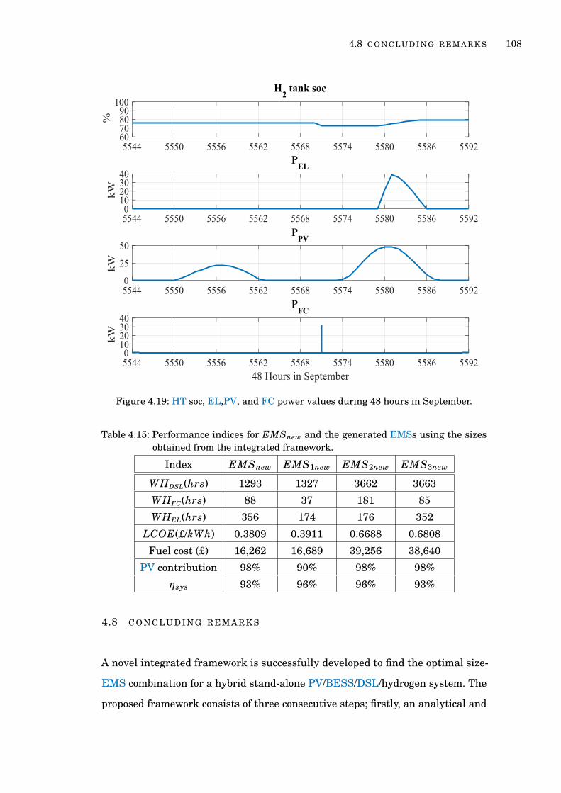
4.8 C O N C L U D I N G R E M A R K S 108
Figure 4.19: HT soc, EL,PV, and FC power values during 48 hours in September.
Table 4.15: Performance indices for EMSnew and the generated EMSs using the sizesobtained from the integrated framework.
Index EMSnew EMS1new EMS2new EMS3new
WHDSL(hrs) 1293 1327 3662 3663
WHFC(hrs) 88 37 181 85
WHEL(hrs) 356 174 176 352
LCOE(£/kWh) 0.3809 0.3911 0.6688 0.6808
Fuel cost (£) 16,262 16,689 39,256 38,640
PV contribution 98% 90% 98% 98%
ηsys 93% 96% 96% 93%
4.8 C O N C L U D I N G R E M A R K S
A novel integrated framework is successfully developed to find the optimal size-
EMS combination for a hybrid stand-alone PV/BESS/DSL/hydrogen system. The
proposed framework consists of three consecutive steps; firstly, an analytical and

4.8 C O N C L U D I N G R E M A R K S 109
economic sizing is performed using an initial EMS to find the initial size of the
HES. Secondly, Finite Automata is utilised to implement the initial EMS and
instantiate various EMSs. A number of simulations are performed to exercise
these EMSs using the initial sizes. A set of performance indices are also calculated
for the instantiated EMSs which are used as entries to the next step. Thirdly,
an evaluation model is implemented to compare the performance indices of the
initial and instantiated EMSs. This evaluation is achieved to determine the best
operating conditions to use them in generating a new EMS. Then, the new EMS
replaces the initial EMS. The analytical and economical sizing is carried out
again to find the new size based on the new EMS.
The integrated framework proved to produce better results in terms of assets
sizing and HES performance when comparing to the AES approach. Such that,
the PV, EL and HT sizes are reduced. The LCOE of the HES is reduced as well
as increasing the PV contribution.

5
M O D I F Y I N G E N E R G Y M A N A G E M E N T U S I N G F U Z Z Y
L O G I C
5.1 I N T R O D U C T I O N
Chapter 4 demonstrated an integrated framework to obtain the optimal size-
EMS for stand-alone HES. The results obtained by the integrated framework
showed minimising in the size of the PV, LCOE of the system, and maximising
the PV contribution. Since the solar radiation and demand have unpredictable
characteristics and they may change for the coming years, including the source
and demand uncertainty in the HES optimization is necessary.
This chapter demonstrates the design of a FLC to detect the variabilities in the
demand and solar radiation and accordingly modify the EMS of the HES. The
work in this chapter is performed on three stages which are illustrated in Fig-
ure 5.1. The first stage is finding the size-EMS combination using the integrated
framework (similar to that described in Chapter 4), and forecasted solar radiation
and demand profiles. This step is vital in order to include any future changes in
solar radiation and demand data. The second stage includes a sensitivity analysis,
considering the new-obtained size of the HES and the real profiles for solar radi-
ation and demand. The sensitivity analysis is conducted by changing the solar
radiation and demand data for one year by ±5% and ±10% to generate 24 scenar-
ios. In the third stage, the FLC is designed depending on the performance indices
generated from the sensitivity analysis scenarios. The performance indices (see
Section 4.6.2) used in the sensitivity analysis are the fuel cost, DSL working
hours, PV contribution. The objective of the FLC is managing the uncertainty in
demand and solar radiation and then modifying the operating conditions of the
DSL, FC, and the EL in the original EMS. For example, the condition responsible
110
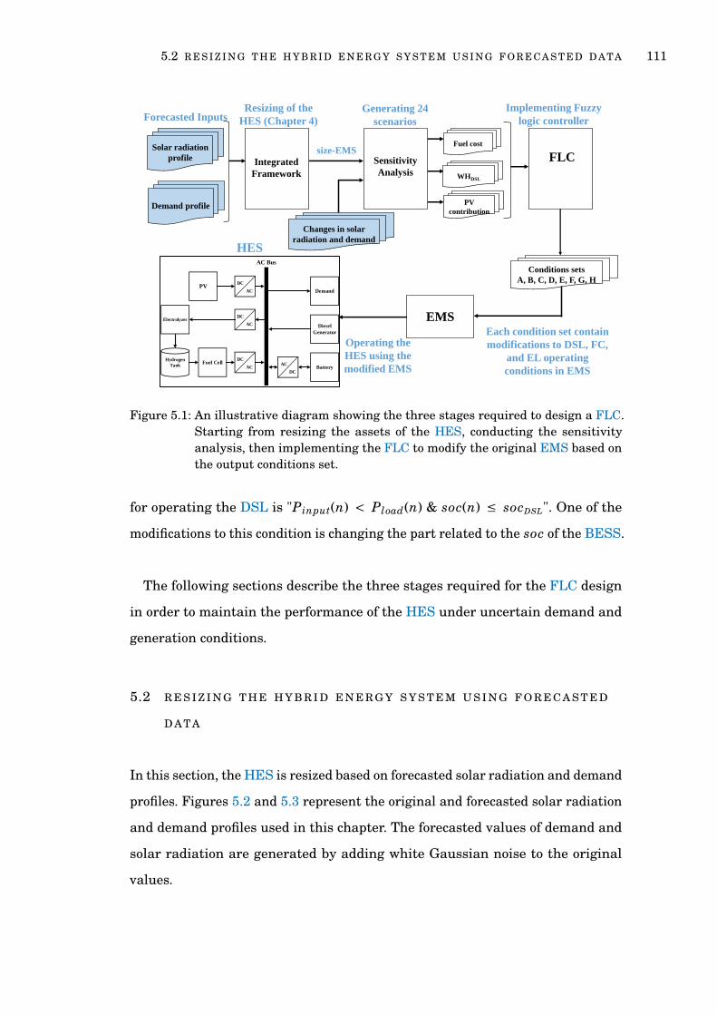
5.2 R E S I Z I N G T H E H Y B R I D E N E R G Y S Y S T E M U S I N G F O R E CA S T E D D ATA 111
Integrated
Framework
Forecasted Inputs
Solar radiation
profile
Resizing of the
HES (Chapter 4)
Changes in solar
radiation and demand
size-EMSSensitivity
Analysis
FLC
Generating 24
scenarios
Conditions sets
A, B, C, D, E, F, G, H
Integrated FrameworkEMS
Fuel cost
WHDSL
PV
contribution
HES
PV
Hydrogen
TankFuel Cell
Battery
Electrolyzer
Diesel
Generator
Demand
DC
AC
DC
ACAC
DC
DC
AC
AC Bus
Demand profile
Each condition set contain
modifications to DSL, FC,
and EL operating
conditions in EMS
Implementing Fuzzy
logic controller
Operating the
HES using the
modified EMS
Figure 5.1: An illustrative diagram showing the three stages required to design a FLC.Starting from resizing the assets of the HES, conducting the sensitivityanalysis, then implementing the FLC to modify the original EMS based onthe output conditions set.
for operating the DSL is "Pinput(n) < Pload(n) & soc(n) ≤ socDSL". One of the
modifications to this condition is changing the part related to the soc of the BESS.
The following sections describe the three stages required for the FLC design
in order to maintain the performance of the HES under uncertain demand and
generation conditions.
5.2 R E S I Z I N G T H E H Y B R I D E N E R G Y S Y S T E M U S I N G F O R E CA S T E D
D ATA
In this section, the HES is resized based on forecasted solar radiation and demand
profiles. Figures 5.2 and 5.3 represent the original and forecasted solar radiation
and demand profiles used in this chapter. The forecasted values of demand and
solar radiation are generated by adding white Gaussian noise to the original
values.

5.2 R E S I Z I N G T H E H Y B R I D E N E R G Y S Y S T E M U S I N G F O R E CA S T E D D ATA 112
Jan Feb Mar Apr May Jun Jul Aug Sep Oct Nov Dec
Figure 5.2: Original and forecasted solar radiation of one calendar year.
Jan Feb Mar Apr May Jun Jul Aug Sep Oct Nov Dec
Figure 5.3: Original and forecasted demand distribution of one calendar year.
Table 5.1 illustrates the sizes of the HES resulting from the integrated frame-
work using the forecasted profiles. Compared to the sizes obtained in Table 4.13

5.3 S E N S I T I V I T Y A N A LY S I S 113
from Chapter 4, it can be noted that the PV size has not changed, while there is
an increase in the DSL, FC and BESS sizes. The size of the EL and HT is fixed.
The original solar radiation and demand profiles are called the base case in the
sensitivity analysis and explained in the following section.
Table 5.1: The optimal size of HES using the integrated framework and forecasted de-mand and solar irradiance.
Subsystem in the HES Obtained size
PV 60 kWBESS 240.54 kWh
EL 50 kWFC 38.55 kW
DSL 38.55 kWHT 45 kg
5.3 S E N S I T I V I T Y A N A LY S I S
A sensitivity analysis is conducted to measure the degree of uncertainty of
demand and solar radiation data. It is performed by an annual change of ±5%
and ±10% of demand and solar values. The performance indices that have been
selected to be checked after carrying out the sensitivity analysis are fuel cost,
WHDSL and PV contribution. These performance indices are chosen since it is
desirable to reduce the DSL working hours and the fuel cost while ensuring
maximum utilisation of PV energy. The variations on demand and solar variation
generate 24 scenarios, and these scenarios are displayed in Tables 5.2 - 5.7.
Table 5.2 presents the results of the sensitivity analysis performed by an annual
change of ±5% and ±10% of the demand only. Scenario 1 shows an increase in the
demand by 5%, causing an increase in the fuel cost, WHDSL, and PV contribution
as well. The increase in fuel cost and WHDSL is expected as the increase in
the demand is partly covered by the DSL. PV energy is also contributed to
supply the demand and that explains the increase in PV contribution. However,
increasing the annual demand by 10% leads to a further increase in those indices.

5.3 S E N S I T I V I T Y A N A LY S I S 114
Table 5.2: Results of sensitivity analysis for an annual change of ±5% and ±10% of Pload.
Scenario No. Description Fuel Cost WHDSL PV Contribution
Base case - £16071 1061 96%
Scenario 1 +5% Pload £17541 1158 98%
Scenario 2 +10% Pload £19131 1263 99%
Scenario 3 -5% Pload £14769 975 93%
Scenario 4 -10% Pload £13481 890 89%
Alternatively, the reduction in demand causes a reduction in the fuel cost, WHDSL
and PV contribution as the request for energy decreased.
In Table 5.3, scenarios 5 to 8 illustrate the performance indices resulted from
changing the solar radiation by ±5% and ±10% of the base case. Increasing solar
radiation causes a reduction in WHDSL and fuel cost. This is due to the increase
PV energy used to supply to the demand, generate H2, and charging BESS.
However, the increase in the PV energy has not been fully exploited leading
to decrease in the PV contribution. On the other hand, the decrease in solar
radiation leads to an increase in WHDSL and hence the fuel cost. Whereas the PV
contribution is increased since the demand has not changed and the generated
PV energy is almost fully utilised.
Table 5.3: Results of sensitivity analysis for an annual change of ± 5% and ± 10% of IPV .
Scenario No. Description Fuel Cost WHDSL PV Contribution
Scenario 5 +5% IPV £15617 1031 93%
Scenario 6 +10% IPV £15147 1000 90%
Scenario 7 -5% IPV £16682 1102 98%
Scenario 8 -10% IPV £17420 1150 100%
Table 5.4 shows the performance indices for the scenarios 9, 10, 11 and 12.
These scenarios are resulted from increasing the annual demand and solar
radiation by 5% and 10%. It can be observed that the highest values of the fuel
cost and PV contribution are for the scenarios where the annual increase in
demand is 10%. While the values for the scenarios with an increase of 5% in the
demand, range around the base case.

5.3 S E N S I T I V I T Y A N A LY S I S 115
Table 5.4: Results of sensitivity analysis for an annual change of +5%, +10% of Pload andIPV .
Scenario No. Description Fuel Cost WHDSL PV Contribution
Scenario 9 +5% Pload, +5% IPV £16950 1119 96%
Scenario 10 +5% Pload, +10% IPV £16450 1086 93%
Scenario 11 +10% Pload, +5% IPV £18404 1215 97%
Scenario 12 +10% Pload, +10% IPV £17783 1174 96%
Table 5.5 presents the sensitivity analysis for an annual increase of 5%, 10% of
the demand and an annual decrease of 5%, 10% of the solar radiation. Generally,
increasing the demand and decreasing solar radiation cause a noticeable rise
in fuel cost and WHDSL. The highest values for the performance indices are for
scenarios 14 and 16 where the increase in demand is 10%.
Table 5.5: Results of sensitivity analysis for an annual change of +5%, +10% of Pload and−5%, −10% of IPV .
Scenario No. Description Fuel Cost WHDSL PV Contribution
Scenario 13 +5% Pload, -5% IPV £18238 1204 99%
Scenario 14 +10% Pload, -5% IPV £19934 1316 100%
Scenario 15 +5% Pload, -10% IPV £19071 1259 100%
Scenario 16 +10% Pload, -10% IPV £20782 1372 100%
On the contrary, decreasing the demand and increasing the solar radiation
in the sensitivity analysis causes a reduction the fuel cost and WHDSL. This
illustrated in Table 5.6 where the demand is decreased by 5% and 10% and solar
radiation is increased by the same percentage. The PV contribution decreases and
this is reasonable since the increment in solar radiation is unexploited because
of the reduction in the demand. The lowest values for fuel cost, WHDSL and PV
contribution are for scenarios 18 and 20 where the decrease in demand is 10%.
Whereas, the decrease in the demand in scenarios 17 and 19 are 5%, so the
reduction in the performance indices is less than for the other two scenarios.
The last four scenarios in sensitivity analysis are presented in Table 5.7. Both
demand and solar radiation are decreased by 5% and 10%. Scenarios from 20

5.3 S E N S I T I V I T Y A N A LY S I S 116
Table 5.6: Results of sensitivity analysis for an annual change of −5%, −10% of Pload,5%, 10% for IPV .
Scenario No. Description Fuel Cost WHDSL PV Contribution
Scenario 17 -5% Pload, +5% IPV £14329 946 90%
Scenario 18 (-10% Pload, +5% IPV £13118 866 86%
Scenario 19 -5% Pload, +10% IPV £13951 921 87%
Scenario 20 -10% Pload, +10% IPV £12754 842 83%
to 24 represent the results obtained from the reduction in demand and solar
radiation.
Table 5.7: Results of sensitivity analysis for an annual change of −5%, −10% of Ploadand IPV .
Scenario No. Description Fuel Cost WHDSL PV Contribution
Scenario 21 -5% Pload, -5% IPV £15223 1005 96%
Scenario 22 -5% Pload, -10% IPV £15844 1046 98%
Scenario 23 -10% Pload, -5% IPV £13921 919 92%
Scenario 24 -10% Pload, -10% IPV £14390 950 96%
Figures 5.4, 5.5 and 5.6 show the 24 scenarios concerning the sensitivity
analysis of the fuel cost, WHDSL and PV contribution, respectively. In Figure 5.4,
the best and worst scenarios regarding fuel cost sensitivity analysis can be
observed. The best scenario happens when the fuel cost is minimum and obtained
by scenario 20 (-10% Pload, +5% IPV ). While the worst scenario is found when
the fuel cost is maximum. This is depicted by scenario 16 where the demand is
increased by 10% and solar radiation is decreased by 10%. Generally, the worst
scenario happens when the increment in demand cannot be covered by the solar
radiation leading to increase the reliance on the DSL.
Figure. 5.5 shows the influence of changing the demand and solar radiation in
the working hours of the DSL. The figure shows the same trend as the fuel cost
in the previous figure. This means when the WHDSL is high this results in higher
fuel cost and vice versa. Accordingly, the best and worst scenarios for this figure
are the same as the ones found by the fuel cost sensitivity analysis. The worst
scenario is 20 and the best scenario is 16.

5.3 S E N S I T I V I T Y A N A LY S I S 117
0
2500
5000
7500
10000
12500
15000
17500
20000
22500
Bas
e ca
se
5%
10%
-5%
-10
%
5%
10%
-5%
-10
%
5%
*,
5%
5%
*,
10%
10%
*,
5%
10%
*,
10
%
5%
*, -5
%
10
%*,
-10%
5%
*, -1
0%
10
%*,
-10
%
-5%
*,
5%
-10
%*
, 5%
-5%
*,
10%
-10
%*
, 10
%
-5%
*,
-5%
-5%
*,
-10
%
-10
%*
, -5
%
-10
%*
, -1
0%
Demand Solar radiation Demand*, solar
radiation
Demand*, solar
radiation
Demand*, solar
radiation
Demand*, solar
radiation
Fuel cost (£)
1
2
34
5 6
78 9
10
1112 13
1415
16
1718
1920
2122
23 24
• Numbers from 1 to 24 represent the
24 sensitivity analysis scenario
Figure 5.4: The effect of demand and solar radiation variations on the fuel cost.
0
200
400
600
800
1000
1200
1400
Bas
e ca
se
5%
10%
-5%
-10
%
5%
10%
-5%
-10
%
5%
*,
5%
5%
*,
10%
10%
*,
5%
10%
*,
10
%
5%
*, -5
%
10
%*,
-10
%
5%
*, -1
0%
10
%*,
-10
%
-5%
*,
5%
-10
%*
, 5%
-5%
*,
10%
-10
%*
, 10
%
-5%
*,
-5%
-5%
*,
-10
%
-1
0%
*,
-5%
-10
%*
, -1
0%
Demand Solar radiation Demand*, solar
radiation
Demand*, solar
radiation
Demand*, solar
radiation
Demand*, solar
radiation
WHDSL
12
3
4
5 6
78
9 10
11 12 13
1416
17
1819
20
21 2223 24
15
• Numbers from 1 to 24 represent the
24 sensitivity analysis scenario
Figure 5.5: The effect of demand and solar radiation variations on DSL working hours.
Finally, the PV contribution sensitivity analysis is clarified by Figure 5.6. It
is most desirable to increase the PV utilisation and this is reflected in the PV
contribution. The best scenarios are when the PV contribution is 100% and they
are 8, 14, 15 and 16. It is noted that all these scenarios happen when solar

5.3 S E N S I T I V I T Y A N A LY S I S 118
0%
10%
20%
30%
40%
50%
60%
70%
80%
90%
100%
110%
Bas
e ca
se
5%
10%
-5%
-10
%
5%
10%
-5%
-10
%
5%
*,
5%
5%
*,
10%
10%
*,
5%
10%
*,
10
%
5%
*, -5
%
10
%*,
-10
%
5%
*, -1
0%
10
%*,
-10
%
-5
%*,
5%
-10
%*
, 5%
-5%
*,
10%
-10
%*
, 10
%
-5%
*,
-5%
-5%
*,
-10
%
-10
%*
, -5
%
-10
%*
, -1
0%
Demand Solar radiation Demand*, solar
radiation
Demand*, solar
radiation
Demand*, solar
radiation
Demand*, solar
radiation
PV contribution
2
34 5 6
7 8 9 10 11 12 13 14 15 16
17 18 19 20
21 22 23 24
• Numbers from 1 to 24 represent the
24 sensitivity analysis scenario
1
Figure 5.6: The effect of demand and solar radiation variations on PV contribution.
radiation is reduced by 10%. This means that when the annual solar radiation is
less, the HES can exploit all the produced PV energy. While the worst scenario
is when the PV contribution is minimum and this is scenario 20. However, this
scenario is considered the best scenario for fuel cost and WHDSL. This is due to
the reduction in the demand by 10% meaning less dependent on the DSL. To
conclude, after the sensitivity analysis is achieved, the variability in the annual
demand has more effect on the DSL working hours and hence fuel cost. While
this relation is the inverse with regard to the PV contribution, as the reduction
in the demand leads to decrease in the PV contribution. This can be explained
as the demand consumes less energy from the PV leading to more losses in PV
energy.
However, the conducted sensitivity analysis is not just for investigating the ef-
fect of the demand and solar radiation uncertainty on the HES performance. The
purpose of the sensitivity analysis is to use the results obtained in implementing
a FLC which is explained in the following section.

5.4 M O D I F Y T H E E M S U S I N G F U Z Z Y L O G I C 119
5.4 M O D I F Y T H E E M S U S I N G F U Z Z Y L O G I C
The results of the sensitivity analysis are exploited to implement a FLC. This con-
troller detects the changes in the demand and solar radiation and consequently
modifies the operating conditions of the DSL, FC, and EL in the EMS. A general
introduction on FLC has been presented in Chapter 2. This section includes the
design of the FLC, description of the fuzzy rules involved, the output of the FLC,
and finally, a case study to verify the effectiveness of the FLC.
5.4.1 The design of Fuzzy Logic Controller
The key objective of the FLC is to modify the operating conditions of the EMS
obtained previously by the integrated framework (see Chapter 4). This gives the
EMS the ability to deal with the uncertainty in inputs. The DSL, FC, and EL in
the HES are the target assets to modify their operating conditions. Operating
these assets has a considerable effect on the BESS and HT charging and discharg-
ing process. The PV is considered ON continuously even if the solar radiation is
zero, so its operating condition has not been modified. The BESS and HT rely on
the above-mentioned assets for charging and discharging. Thus any change in
the operating conditions of the DSL, FC, and EL will affect their performance.
Figure 5.7 shows the configuration of the FLC that clearly illustrates the three
steps of the FLC.
The results of the sensitivity analysis are used in the implementation of a FLC.
Thereby, the fuel cost, WHDSL, and the PV contribution of the 24 scenarios in
Tables 5.2 to 5.7 are considered the inputs to the FLC. The input variables are
fuzzified into membership functions. These membership functions are basically
fuzzy sets and the degree of membership of a value is defined as how much this
value is close to that set. Table 5.8 introduces the fuzzy sets that define the
membership functions. The fuzzy sets are divided into three ranges: LOW, MED,
and MAX. The LOW fuzzy set contains the lowest values, while the MED fuzzy

5.4 M O D I F Y T H E E M S U S I N G F U Z Z Y L O G I C 120
Fuzzy
Logic
Controller
Fuel cost
WHDSL
PV contribution
Conditions sets
Figure 5.7: The configuration of the FLC introducing the input membership functions;fuel cost, WHDSL, and PV contribution. The output membership function isthe conditions sets that modify the EMS.
set is intermediate between the lowest and the highest values. The MAX fuzzy
set covers the highest values of the selected performance indices.
Figure 5.8 presents the membership function for the fuel cost input fuzzy set.
Figures 5.9 and 5.10 illustrate the membership functions for the WHDSL and PV
contribution input fuzzy sets.
After determining the input fuzzy sets ( i.e., fuel cost, WHDSL, and PV contri-
bution), the 24 sensitivity analysis scenarios can be classified into LOW, MED
and MAX.
Table 5.9 defines each scenario in terms of fuzzy sets. By observing the fuzzy
inputs in the table, it can be recognised that some scenarios share the same fuzzy
sets. For example, scenarios 1, 8, 9, 11, 12, and 13 share the same input fuzzy
Table 5.8: Numerical ranges of the fuzzy sets
Fuel cost (£)LOW MED MAX
12000-16000 15000-19000 18000-21000
WHDSL (hours)LOW MED MAX
800-1100 1000-1300 12000-1500
PV contribution (%)LOW MED MAX80-91 90-96 95-100

5.4 M O D I F Y T H E E M S U S I N G F U Z Z Y L O G I C 121
Figure 5.8: Membership function for fuel cost input fuzzy set.
sets (MED, MED, and MAX). Grouping the scenarios that have the same input
Figure 5.9: Membership function for WHDSL input fuzzy set.

5.4 M O D I F Y T H E E M S U S I N G F U Z Z Y L O G I C 122
Figure 5.10: Membership function for PV contribution input fuzzy set.
fuzzy sets results in eight groups of scenarios. As a result, the fuzzy rules for the
FLC are eight rules.
Table 5.10 represents the relationship between the sensitivity analysis sce-
narios, the ranges of the output fuzzy sets and the symbols that represent the
conditions sets. The first column shows the scenarios with similar input fuzzy
sets. Based on this similarity, the number of fuzzy rules needed for the FLC can
be stated and equals to 8 rules. The output fuzzy sets represent the number of
scenarios that have similar fuzzy input sets. The range for each output fuzzy
set (i.e., third column) is the total number of scenarios that have similar input
fuzzy sets (i.e., second column). The last column in the table is the symbols of the
conditions sets representing the output fuzzy sets. To illustrate, scenarios 1, 8, 9,
11, 12, an 13 belong to the range [0 - 7] which is the output fuzzy set A. It should
be noted that the number of scenarios is 6, while the range is [0 - 7], this due to
the overlapping of fuzzy output sets. While scenarios 2, 14, 15, and 16 belong to
the range [6 - 11] that is the output fuzzy set B, and so on. These output fuzzy

5.4 M O D I F Y T H E E M S U S I N G F U Z Z Y L O G I C 123
Table 5.9: The 24 sensitivity analysis scenarios interpreted into LOW, MED, and MAXwith regarding to the fuzzy sets.
Scenario No. Fuel Cost WHDSL PV Contribution
Scenario 1 MED MED MAX
Scenario 2 MAX MAX MAX
Scenario 3 LOW LOW MED
Scenario 4 LOW LOW LOW
Scenario 5 MED LOW MED
Scenario 6 LOW LOW LOW
Scenario 7 MED LOW MAX
Scenario 8 MED MED MAX
Scenario 9 MED MED MAX
Scenario 10 MED MED MED
Scenario 11 MED MED MAX
Scenario 12 MED MED MAX
Scenario 13 MED MED MAX
Scenario 14 MAX MAX MAX
Scenario 15 MAX MAX MAX
Scenario 16 MAX MAX MAX
Scenario 17 LOW LOW LOW
Scenario 18 LOW LOW LOW
Scenario 19 LOW LOW LOW
Scenario 20 LOW LOW LOW
Scenario 21 LOW LOW MAX
Scenario 22 MED LOW MAX
Scenario 23 LOW LOW MED
Scenario 24 LOW LOW MAX
sets are translated into condition sets that replace the previous conditions in the
original EMS (see Section 4.6.3) to improve the performance of HES.
These conditions sets represent the modifications made to the operating con-
ditions of the FC, DSL, and EL. Each set of conditions modifies the operating
conditions of one or more of the DSL, FC, and EL. An explanation of the condi-
tions sets from A to H is presented in the following section.

5.4 M O D I F Y T H E E M S U S I N G F U Z Z Y L O G I C 124
Table 5.10: Illustration of the relationship between the sensitivity analysis scenarios, theoutput fuzzy sets and the condition sets.
ScenarioSum of
ScenariosOutput Fuzzy
Set RangesOutput FuzzySets Symbols
1, 8, 9, 11, 12, 13 6 [0 - 7] A
2, 14, 15, 16 4 [6 - 11] B
3, 23 2 [10 - 13] C
4, 6, 17, 18, 19, 20 6 [12 - 19] D
5 1 [18 - 20] E
7, 22 2 [19 - 21] F
10 1 [20 - 22] G
21, 24 2 [21 - 24] H
Figure 5.11: Membership function for output fuzzy sets.
5.4.2 The Fuzzy Rules
In the previous section, the input fuzzy sets are identified which are the fuel
cost, working hours of the DSL, and the PV contribution. In addition, it has been
clarified why the fuzzy rules needed are equal to eight rules. In this section, the

5.4 M O D I F Y T H E E M S U S I N G F U Z Z Y L O G I C 125
fuzzy rules are explained in detail. Tables 5.11 and 5.12 represent the operating
conditions of EMSnew obtained by the integrated framework and values related
to BESS soc and HT socHT (see Chapter 4). These tables have been listed in
this section to investigate the effectiveness of the designed FLC on the EMS.
In Table 5.11, DSL operation is controled by Conditions 14 and 15. Conditions
16, 17, and 18 responsible for EL operation. While conditions 19 - 22 are for the
FC operation. These operating conditions can be modified to improve the HES
performance when there are uncertainty in the demand and solar radiation.
Table 5.11: Operating conditions for EMSnew produced by the integrated frameworkdescribed in Chapter 4.
Condition No. Description Operating Conditions
10 BESS chargingPinput(n) ≥ Pload(n)& soc(n) < socmax
11 BESS OFF soc(n) ≥ socmax
12 BESS dischargingPinput(n) < Pload(n)& soc(n) > socDSL
13 BESS OFF soc(n) ≤ socmin
14 DSL ONPinput(n)< Pload(n)
& soc(n)≤ socDSL & BFC = 0
15 DSL OFF Pinput(n) > Pload(n)
16 EL ON0< PPV ,surplus(n)< PEL,min
& socHT(n)< socHTmax
& soc(n)> socmin
17 EL OFF PPV ,surplus(n)= 0
18 EL OFF socHT(n) ≥ socHTmax
19 FC ON
Pinput(n)< Pload(n)& socFC < soc(n)≤ 40%
& socHT(n)> socHTmin
& BFC(n−1)= 1
20 FC ONPinput(n)< Pload(n)
& soc(n)≤ socFC
& socHT(n)> socHTmin
21 FC OFF soc(n) > socFC
22 FC OFF socHT(n) ≤ socHTmin

5.4 M O D I F Y T H E E M S U S I N G F U Z Z Y L O G I C 126
Table 5.12: Values of the parameters related to soc and socHT mentioned in Table 5.11.
Parameter Value Parameter Value
socmin 20% socmax 80%
socFC 35% socDSL 25%
socHTmin 10% socHTmin 90%
Table 5.13 defines the changes made to the operating conditions of the FC,
DSL and EL introduced in Table 5.11. The conditions sets are labeled from A
to H, condition sets B, D and G are modifying the operating conditions of DSL,
FC, and EL. Whereas the other sets are modifying the operating conditions of
DSL and FC. DSL is the only asset among the others that has been modified
in all conditions sets. The modifications done on the FC operating condition are
targeting the part related to the soc and socHT. The first part of the condition
that is dealing with the demand remained unchanged.
The derivation of the fuzzy rules is based on our experience and a series of
simulations. The changes are summarized as follows:
1. The soc in the DSL operating condition for all the sets from A to H has been
changed to: soc(n) ≤ socFC & socHT(n) > socHTmin. This ensures more
utilisation of BESS energy.
2. Condition set A: the FC operating condition has been changed to
soc(n) ≤ socFC & socHT(n) > socHTmin OR soc(n) = socmax &
socHT(n) ≤ socHTmax. This condition allows the FC to operate when-
ever the soc is less than 35% without hysteresis zone. However, the FC
also operates when the BESS is fully charged after checking the availabil-
ity of H2. The power generated by the FC supplies the demand without
generating any surplus.
3. Condition set B: the condition soc(n) = socmax & socHT(n) ≤ socHTmax
has been added to the FC operating condition. This allows the FC to operate
when the BESS is fully charged and the power generated by the FC supplies
the demand without generating any surplus.

5.4 M O D I F Y T H E E M S U S I N G F U Z Z Y L O G I C 127
Table 5.13: The sets of modified conditions labeled from A to H.
Condition Sets Symbols Operating Conditions
ADSL: soc(n) ≤ socmin & BFC(n) = 0
FC: soc(n) ≤ socFC & socHT(n) > socHTmin
OR soc(n) = socmax & socHT(n) ≤ socHTmax
B
DSL: soc(n) ≤ socmin & BFC(n) = 0
FC: socFC ≤ soc(n) < 40%
& socHT(n) > socHTmin & BFC(n−1) = 1
OR soc(n) ≤ socFC & socHT(n) > socHTmin
OR soc(n) = socmax & socHT(n) ≤ socHTmax
EL: 85% ≤ soc(n) < socHTmax
& socHT(n−1) < socHTmax & PPV ,surplus(n) = 0
CDSL: soc(n) ≤ socmin & BFC(n) = 0
FC: 50% < soc(n) ≤ 70%
& socHT(n) > socHTmin & BFC(n−1) = 1
OR soc(n) ≤ 50% & socHT(n) > socHTmin
D
DSL: soc(n) ≤ socmin & BFC(n) = 0
FC: 50% < soc(n) ≤ 70%
& socHT(n) > socHTmin& BFC(n−1) = 1
OR soc(n) ≤ 50% & socHT(n) > socHTmin
EL: 85% < soc(n) ≤ socmax
& socHT(n−1) < socHTmax
& PPV ,surplus(n) = 0
EDSL: soc(n) ≤ socmin & BFC(n) = 0
FC: 30% < soc(n) < 40%
& socHT(n) > socHTmin & BFC(n−1) = 1
OR soc(n) ≤ 30% & socHT(n) > socHTmin
Continued on next page

5.4 M O D I F Y T H E E M S U S I N G F U Z Z Y L O G I C 128
Table 5.13 – continued from previous page
Condition Sets Symbols Operating Conditions
FDSL: soc(n) ≤ socmin & BFC(n) = 0
FC: 30% ≤ soc(n) < 40%
& socHT(n) > socHTmin & BFC(n−1) = 1)
OR soc(n) ≤ 30% & socHT(n) > socHTmin)
OR soc(n) = socmax & socHT(n) ≤ socHTmax
G
DSL: soc(n) ≤ socmin & BFC(n) = 0
FC: 70% < soc(n) ≤ socmax
& socHT(n) > socHTmin
EL: 85% < soc(n) < socmax
& socHT(n−1) < socHTmax & PPV ,surplus(n) = 0
H
DSL: soc(n) ≤ socmin
& BFC(n) = 0
FC: 70% < soc(n) ≤ socmax
& socHT(n) > socHTmin
4. Condition set C: the soc ranges for the FC operating condition related
to hysteresis zone has been changed to 50% and 70% and the following
condition has been added: soc(n) ≤ 50% & socHT(n) > socHTmin. This
means the FC operates when the BESS is charged to the half. In simulation
this proves to reduce the DSL working hours.
5. Condition set D:
• the changes made to the FC operating conditions are the same as in
condition set C.
• the EL operating condition has been changed to:
85% < soc(n) ≤ socmax
& socHT(n−1) < socHTmax & PPV ,surplus(n) = 0. The EL operates

5.4 M O D I F Y T H E E M S U S I N G F U Z Z Y L O G I C 129
when the BESS soc between 85% and socmax and there surplus PV
energy equals to zero. This permits the BESS to operate the EL
leading to generate more H2.
6. Condition set E: the socFC in the FC operating condition has been changed
from 35% to 30% to exploit more energy from the BESS.
7. Condition set F: the socFC in the FC operating condition from
has been changed from 35% to 30% (same as in condition
set E). In addition, the following condition has been added:
soc(n) = socmax & socHT(n) ≤ socHTmax, which the same as in
condition set B.
8. Condition set G:
• the second part of the FC operating condition has been changed to:
70% < soc(n) ≤ socmax & socHT(n) > socHTmin. This means the
FC operates if the soc of the BESS is between 70% and socmax. The
power generated by the FC supplies the demand without generating
any surplus.
• the changes that has been made to the EL operating condition is the
same as in condition set D.
9. Condition set H: the changes that has been made to the FC operating
condition are the same as in condition set G.
The fuzzy rules that determine the relationship between the fuzzy inputs and
fuzzy outputs are outlined as follow:
• If (Fuel cost ∈ MED) and (WHDSL ∈ MED) and (PV contribution ∈ MAX)
then (output = A).
• If (Fuel cost ∈ MAX) and (WHDSL ∈ MAX) and (PV contribution ∈ MAX)
then (output = B).
• If (Fuel cost ∈ LOW) and (WHDSL ∈ LOW) and (PV contribution ∈ MED)
then (output = C).
• If (Fuel cost ∈ LOW) and (WHDSL ∈ LOW) and (PV contribution ∈ LOW)
then (output = D).

5.4 M O D I F Y T H E E M S U S I N G F U Z Z Y L O G I C 130
• If (Fuel cost ∈ MED) and (WHDSL ∈ LOW) and (PV contribution ∈ MED)
then (output = E).
• If (Fuel cost ∈ MED) and (WHDSL ∈ LOW) and (PV contribution ∈ MAX)
then (output = F).
• If (Fuel cost ∈ MED) and (WHDSL ∈ MED) and (PV contribution ∈ MED)
then (output = G).
• If (Fuel cost ∈ LOW) and (WHDSL ∈ LOW) and (PV contribution ∈ MAX)
then (output = H).
After determining the input fuzzy sets and the rules, the following section intro-
duces the output fuzzy sets and the results obtained after applying the FLC. In
addition, a comparison has been done to highlight the improvements on the HES
made by the FLC.
5.4.3 The Results of Fuzzy Logic Controller
The main aim of the FLC is to modify the EMS of the HES to overcome the
uncertainty in demand and solar radiation dataset. This is achieved by modifying
some of the operating conditions to decrease working hours and fuel cost of
the DSL and also increase the PV contribution. The FLC is designed using
the Fuzzytool supported by MATLAB. The output of the FLC is a number of
conditions sets alphabetically labelled from A to H. Depending on the input
fuzzy sets, each output fuzzy set (i.e., each set of conditions) replaces the original
conditions in the EMS to generate a modified EMS. In this chapter, the operating
conditions of the DSL, FC, and EL are the only conditions that supposed to be
affected by the FLC (see Section 5.4.1).
Table 5.14 summarizes the output of the FLC for the 24 scenarios introduced
by the sensitivity analysis. To evaluate the impact of applying the modified EMS
on the performance of the HES, a comparison between the performance indices
has been performed. This is illustrated in Figures 5.12, 5.13, and 5.14.
Figure 5.12 shows the values of the fuel cost for the 24 scenarios before and after
applying the FLC. In general, it is observed that there are noticeable reductions
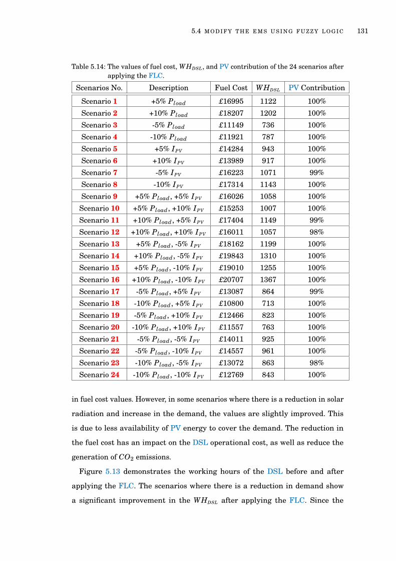
5.4 M O D I F Y T H E E M S U S I N G F U Z Z Y L O G I C 131
Table 5.14: The values of fuel cost, WHDSL, and PV contribution of the 24 scenarios afterapplying the FLC.
Scenarios No. Description Fuel Cost WHDSL PV Contribution
Scenario 1 +5% Pload £16995 1122 100%
Scenario 2 +10% Pload £18207 1202 100%
Scenario 3 -5% Pload £11149 736 100%
Scenario 4 -10% Pload £11921 787 100%
Scenario 5 +5% IPV £14284 943 100%
Scenario 6 +10% IPV £13989 917 100%
Scenario 7 -5% IPV £16223 1071 99%
Scenario 8 -10% IPV £17314 1143 100%
Scenario 9 +5% Pload, +5% IPV £16026 1058 100%
Scenario 10 +5% Pload, +10% IPV £15253 1007 100%
Scenario 11 +10% Pload, +5% IPV £17404 1149 99%
Scenario 12 +10% Pload, +10% IPV £16011 1057 98%
Scenario 13 +5% Pload, -5% IPV £18162 1199 100%
Scenario 14 +10% Pload, -5% IPV £19843 1310 100%
Scenario 15 +5% Pload, -10% IPV £19010 1255 100%
Scenario 16 +10% Pload, -10% IPV £20707 1367 100%
Scenario 17 -5% Pload, +5% IPV £13087 864 99%
Scenario 18 -10% Pload, +5% IPV £10800 713 100%
Scenario 19 -5% Pload, +10% IPV £12466 823 100%
Scenario 20 -10% Pload, +10% IPV £11557 763 100%
Scenario 21 -5% Pload, -5% IPV £14011 925 100%
Scenario 22 -5% Pload, -10% IPV £14557 961 100%
Scenario 23 -10% Pload, -5% IPV £13072 863 98%
Scenario 24 -10% Pload, -10% IPV £12769 843 100%
in fuel cost values. However, in some scenarios where there is a reduction in solar
radiation and increase in the demand, the values are slightly improved. This
is due to less availability of PV energy to cover the demand. The reduction in
the fuel cost has an impact on the DSL operational cost, as well as reduce the
generation of CO2 emissions.
Figure 5.13 demonstrates the working hours of the DSL before and after
applying the FLC. The scenarios where there is a reduction in demand show
a significant improvement in the WHDSL after applying the FLC. Since the

5.4 M O D I F Y T H E E M S U S I N G F U Z Z Y L O G I C 132
0
2500
5000
7500
10000
12500
15000
17500
20000
22500
5%
10%
-5%
-10
%
5%
10%
-5%
-10
%
5%
*,
5%
5%
*,
10
%
10%
*,
5%
10%
*,
10
%
5%
*, -5
%
10
%*
, -1
0%
5%
*, -1
0%
10
%*
, -1
0%
-5%
*,
5%
-10
%*
, 5%
-5
%*,
10%
-10
%*
, 10
%
-5%
*,
-5%
-5%
*,
-10
%
-10
%*
, -5
%
-10
%*
, -1
0%
Demand Solar radiation Demand*, solar
radiation
Demand*, solar
radiation
Demand*, solar
radiation
Demand*, solar
radiation
Fuel Cost (£)Before FLC After FLC
Figure 5.12: The fuel cost before and after applying the FLC.
0
200
400
600
800
1000
1200
1400
5%
10%
-5%
-10
%
5%
10%
-5%
-10
%
5%
*,
5%
5%
*,
10
%
10%
*,
5%
10%
*,
10
%
5%
*, -5
%
10
%*,
-10
%
5%
*, -1
0%
10
%*,
-10
%
-5%
*,
5%
-10
%*
, 5%
-5%
*,
10
%
-10
%*
, 10
%
-5%
*,
-5%
-5%
*,
-10
%
-10
%*
, -5
%
-10
%*
, -1
0%
Demand Solar radiation Demand*, solar
radiation
Demand*, solar
radiation
Demand*, solar
radiation
Demand*, solar
radiation
WHDSL Before FLC After FLC
Figure 5.13: The DSL working hours before and after applying the FLC.
reduction in demand making the DSL to operate less hours. Overall, the FLC

5.4 M O D I F Y T H E E M S U S I N G F U Z Z Y L O G I C 133
has reduced the DSL working hours leading to reduce the replacement costs of
the DSL.
Figure 5.14 illustrates the improvements in the PV contribution after applying
the FLC. It is observed that for most of the scenarios, the PV contribution has
been raised to 100%. There are a group of scenarios that have 100% utilisation of
PV before applying the FLC. Such as, scenario 14 (+10% Pload, -5% IPV ), 15 (+5%
Pload, -10% IPV ), and 16 (+10% Pload, -10% IPV ). However, the improvements
that have been made by the FLC yielded in exploiting the PV energy to the
maximum.
0%
10%
20%
30%
40%
50%
60%
70%
80%
90%
100%
110%
5%
10%
-5%
-10
%
5%
10%
-5%
-10
%
5%
*,
5%
5%
*,
10
%
10%
*,
5%
10%
*,
10
%
5%
*, -5
%
10
%*
, -1
0%
5%
*, -1
0%
10
%*
, -1
0%
-5%
*,
5%
-1
0%
*,
5%
-5
%*
, 1
0%
-10
%*
, 10
%
-5
%*,
-5%
-5%
*,
-10
%
-1
0%
*,
-5%
-10
%*
, -1
0%
Demand Solar radiation Demand*, solar
radiation
Demand*, solar
radiation
Demand*, solar
radiation
Demand*, solar
radiation
PV ContributionBefore FLC After FLC
Figure 5.14: The percentage of the PV contribution before and after applying the FLC.
5.4.4 Validation Case Study
To validate the benefits of using the FLC, a case study is implemented for stand-
alone HES. This HES is introduced in Chapter 4 and consists of PV, BESS, DSL,
FC, EL, and HT. The size of the assets in the HES are presented in Section 5.2.
This case study shows the improvements in the performance of the HES before

5.4 M O D I F Y T H E E M S U S I N G F U Z Z Y L O G I C 134
and after applying the FLC. The FLC aims at replacing the operating conditions
of the DSL, FC, and EL by modified conditions. Therefore, the performance of the
HES is enhanced in terms of reliability and cost. Several scenarios are selected
from the 24 sensitivity analysis scenarios to demonstrate the effect of applying
the FLC on the HES performance. Table 5.15 describes the selected scenarios
with the performance indices before and after applying the FLC.
The scenarios selected for the case study are 2, 8, 11, 16, 18, and 24. These
scenarios have been chosen to include various changes in demand and solar
radiation (see Table 5.14). Scenario 2 indicates an annual increase in demand
values by +5%. When comparing the performance indices for this scenario before
and after applying the FLC, it is observed a reduction in the fuel cost by £ 924.
Also the WHDSL is decreased by 61 hours/year. On the other hand, there is a
considerable increase in FC working hours. The WHFC has increased by 437
hours/year. This is due to the modified condition of the FC obtained by conditions
set B (see Table 5.10). This condition allows the FC to operate more than previ-
ously (see Table 5.13), leading to an increase in the FC working hours. The WHEL
has increased by 47 hours/year, as the modified condition for the EL enables the
operation of the EL when the soc is higher than 85%. Although the decrease
in the WHDSL for this scenario is not significant compared to the base case (see
Table 5.14), however, the improvement achieved is better than before.
Scenario 16 represents the worst case of all the sensitivity analysis scenarios.
The demand values decreased by 10% and the solar radiation values increased
by 10%. Before applying the FLC, the performance indices of this scenario are
considered the highest among the other scenarios. The improvements in these
indices after applying the FLC are minor. For instance, the fuel cost value de-
creased by £ 75, and the WHDSL reduced by 5 hours/year. The other performance
indices such as WHFC and WHEL increased by 5 hours/year.

5.4 M O D I F Y T H E E M S U S I N G F U Z Z Y L O G I C 135
Tabl
e5.
15:D
iffe
rent
scen
ario
sus
edfo
rth
eca
sest
udy
show
ing
the
effe
ctiv
enes
sof
appl
ying
the
FL
C.
Scen
ario
Bef
ore
FL
CA
fter
FL
CF
uel
cost
(£)
WH
DS
L
(hrs
./yea
r)W
HF
C
(hrs
./yea
r)W
HE
L
(hrs
./yea
r)P
Vco
ntr.
Fue
lco
st(£
)
WH
DS
L
(hrs
./yea
r)W
HF
C
(hrs
./yea
r)W
HE
L
(hrs
./yea
r)P
Vco
ntr.
Scen
ario
2+1
0%P
load
1913
112
6375
336
99%
1820
712
0251
238
310
0%
Scen
ario
8-1
0%I P
V17
420
1150
6430
910
0%17
314
1143
6028
910
0%
Scen
ario
11+1
0%P
load
+5%
I PV
1840
412
1578
334
97%
1740
411
4952
438
499
%
Scen
ario
16+1
0%P
load
-10%
I PV
2078
213
7251
255
100%
2070
713
6755
261
100%
Scen
ario
18-1
0%P
load
+5%
I PV
1311
886
655
246
86%
1080
071
338
656
610
0%
Scen
ario
24-1
0%P
load
-10%
I PV
1439
095
060
279
96%
1276
984
311
542
210
0%

5.5 C O N C L U D I N G R E M A R K S 136
5.5 C O N C L U D I N G R E M A R K S
This chapter shows an investigation into modifying the EMS with the presence
of uncertain demand and generation conditions. This investigation involves
conducting a sensitivity analysis to generate several scenarios over a variation
of ±5% and ±10% of demand and solar radiation. These scenarios have been
utilised in implementing a FLC. The objective of such controller is managing
the variations in the demand and solar radiation by modifying the operating
conditions of the DSL, FC, and EL. Several scenarios were compared before
and after applying the FLC. The results obtained show an improvement in the
performance of the HES for most of the variations in the demand and solar
radiation. The data used here (solar radiation and demand) are forecasted using
Gaussian noise and done with MATLAB. In reality, the changes in these data may
be unexpected. Therefore, as a future work, forecasted algorithms that provide
accurate data will be used.
6C O N C L U S I O N S A N D F U T U R E W O R K
6.1 S U M M A R Y A N D C O N C L U S I O N S
Microgrids have emerged to facilitate the integration of Renewable Energy Re-
sources (RERs) and Energy Storage Systems (ESSs) in the traditional distribu-
tion systems. Effective use of diverse RER can provide a strong base for sus-
tainable development, therefore, careful selection of the RERs and managing
their operation are fundamental. This thesis aimed to investigate into sizing
and energy management strategies of microgrids. The assets of a microgrid,
whether grid-connected or stand-alone, have been sized from an economic point
of view. The development of an efficient Energy Management Strategy (EMS) has
been performed to reduce operational costs with ensuring continuous demand
satisfaction. This section summarizes the main conclusions derived from this
thesis.
Sizing of distributed energy resources plays a vital role in microgrid design. It
offers the appropriate size of each asset to obtain the optimal microgrid operation.
In the literature, various methods are used for sizing the microgrid assets, such as
graphical construction, analytical, probabilistic, iterative, artificial intelligence,
hybrid, and software tools. None of these methods could achieve better optimisa-
tion than the other methods on all types of problems (see Chapter 2). However, in
this thesis, the analytical method was selected as the main method for the sizing
of a grid-connected and stand-alone microgrids. Analytical methods have been
widely applied in the literature for their capability in providing accurate results.
Additionally, implementing an effective energy management strategy is critical
to maintaining the balance between generation and demand. Determining the
best size-EMS combination emerges from the significance of achieving a reliable,
137

6.1 S U M M A R Y A N D C O N C L U S I O N S 138
cost-effective, and environmentally friendly microgrid design. The key features
and limitations of research efforts to date in the domain of sizing methods and
energy management strategies are summarised in this thesis (see Chapter 2).
An Analytical and Economic Sizing (AES) was implemented to obtain the
optimal size of a grid-connected Photovoltaic (PV)-Battery Energy Storage System
(BESS). Three types of BESSs are considered and the most economic combination
of PV-BESS has been selected. To evaluate the microgrid with the BESSs, three
case studies have been assessed and the results have shown the combination
PV-Redox Flow Battery (RFB) is the most cost-effective and reliable system.
Moreover, the performance of the PV-RFB combination has been examined with
reference to two different scenarios; when the demand depends completely on
the grid and when the PV only is installed in the microgrid. The results obtained
have indicated that the combination PV-RFB outperforms the other scenarios.
The AES approach is further developed to be included in the integrated frame-
work for sizing stand-alone Hybrid Energy System (HES). The proposed frame-
work aims at finding the optimal size-EMS of a HES. The modified AES is
responsible for determining an initial size of the HES based on initial EMS.
Then, Finite Automata (FA) has been utilised to implement the initial EMS and
instantiate multiple EMSs. These EMSs share the basic characteristics of the
initial EMS with modifying the operating condition of the diesel generator, fuel
cell and electrolyser operation. An evaluation model has been developed to assess
the EMSs and select the featured conditions based on computed performance
indices. The selected operating conditions are then used to form an improved
EMS that replaces the initial one. Following that, the AES has been used to find
the new size of the HES with the improved EMS. The results obtained by the
proposed framework demonstrate a reduction in the cost, PV energy loses, and
the size of the PV system to the half (see Chapter 4).
A Fuzzy Logic Controller (FLC) has been implemented to address the uncer-
tainty in demand and solar radiation. The main aim of this controller is to detect
the changes in input data and accordingly modify the operating conditions of
the Diesel Generator (DSL), Fuel Cell (FC), and Electrolyser (EL). The FLC is
6.2 C R I T I CA L R E V I E W A N D F U T U R E W O R K 139
utilised as a decision maker to keep the HES performance within an acceptable
level regardless of the changes in the input data. A sensitivity analysis has been
carried out generating several scenarios. The performance indices of the gener-
ated scenarios have been used to determine the input fuzzy sets. The obtained
results have demonstrated an improvement in the performance of the HES for
most of the scenarios involved (see Chapter 5).
6.2 C R I T I CA L R E V I E W A N D F U T U R E W O R K
The objectives of this thesis include opening a new research horizons for sizing
and energy management of microgrids. Therefore, many research directions can
be drawn and motivated from this thesis to achieve more performance and energy
efficiency. The limitations of this work and directions for future research are
discussed as follows:
• Acquiring real datasets: the PV profiles used in this thesis are real datasets,
however, the demand profiles employed with the AES to size a grid-
connected microgrid are not. It was a challenge to obtain the real demand
profiles for the Isle of Wight. Requesting the required demand profiles
needs time and usually are not free of charge. However, in future work,
including real datasets in the simulations can provide more reliable results.
• Finite automata tools: the FA used for implementing EMS has been per-
formed using Simulink/state flow. However, there are available tools that
can offer an automated procedure for generating multiple EMSs. This is
will allow to accelerate the process of modelling EMS using FA and can
go further step by including more iterations in the integrated framework.
Examples on these tools are TCT [99] and PHAVer [164].
• Complexity and performance issues: the hydrogen system of the HES (FC,
EL, and Hydrogen Tank (HT)) has not been considered in the calculations
of the Levelised Cost of Energy (LCOE). Including the hydrogen system in
the LCOE computations will increase the complexity of the simulations and

6.2 C R I T I CA L R E V I E W A N D F U T U R E W O R K 140
the AES will not be able to deal with the large number of parameters. In
future work, Artificial Intelligence (AI) or hybrid methods could be explored
to overcome the complexity resulted from increasing the number of assets
in the microgrid.
We believe that the research outcomes generated by this thesis will be useful
for the area of microgrid design, and continue to inspire further research and
development in the above-mentioned directions.

Part II
Thesis Bibliography
141

B I B L I O G R A P H Y
[1] “U.s. securities and exchange commission / captial markets day.”
https://www.sec.gov/. [Online; accessed August-2017].
[2] NREL, “Pv watts calculator.” http://pvwatts.nrel.gov/pvwatts.php. Accessed
10.05.2017.
[3] OpenEI, “Us department of energy.” http://en.openei.org/doe-
opendata/dataset/commercial-and-residential-hourly-load-profiles-
for-all-tmy3-locations-in-the-united-states/. Accessed 10.05.2017.
[4] “Pvwatts calculator.” http://pvwatts.nrel.gov/. [Online; accessed
December-2017].
[5] “Customer-led network revolution.” http://www.networkrevolution.co.
uk/project-library. [Online; accessed Februry-2018].
[6] S. Sinha and S. Chandel, “Review of recent trends in optimization tech-
niques for solar photovoltaic-wind based hybrid energy system,” Renewable
and Sustainable Energy Reviews, vol. 50, pp. 755 – 769, 2015.
[7] B. Bhandari, K.-T. Lee, G.-Y. Lee, Y.-M. Cho, and S.-H. Ahn, “Optimization
of hybrid renewable energy power systems: A review,” International Jour-
nal of Precision Engineering and Manufacturing-Green Technology, vol. 2,
pp. 99–112, Jan 2015.
[8] F. A. Khan, N. Pal, and S. Saeed, “Review of solar photovoltaic and wind
hybrid energy systems for sizing strategies optimization techniques and
cost analysis methodologies,” Renewable and Sustainable Energy Reviews,
vol. 92, pp. 937 – 947, 2018.
[9] K. Anoune, M. Bouya, A. Astito, and A. B. Abdellah, “Sizing methods
and optimization techniques for pv-wind based hybrid renewable energy
system: A review,” Renewable and Sustainable Energy Reviews, vol. 93,
pp. 652 – 673, 2018.
142

B I B L I O G R A P H Y 143
[10] Y. Khawaja, D. Giaouris, H. Patsios, and M. Dahidah, “Optimal cost-based
model for sizing grid-connected pv and battery energy system,” in 2017
IEEE Jordan Conference on Applied Electrical Engineering and Computing
Technologies (AEECT), pp. 1–6, 2017.
[11] R. Hosseinalizadeh, H. S. G, M. Amalnick, and P. Taghipour, “Economic
sizing of a hybrid (PV/WT/FC) renewable energy system (HRES) for stand-
alone usages by an optimization-simulation model: Case study of iran,”
Renewable and Sustainable Energy Reviews, vol. 54, pp. 139–150, 2016.
[12] M. Mehrpooya, M. Mohammadi, and E. Ahmadi, “Techno-economic-
environmental study of hybrid power supply system: A case study in iran,”
Sustainable Energy Technologies and Assessments, vol. 25, pp. 1 – 10, 2018.
[13] A. Hirsch, Y. Parag, and J. Guerrero, “Microgrids: A review of technologies,
key drivers, and outstanding issues,” Renewable and Sustainable Energy
Reviews, vol. 90, pp. 402 – 411, 2018.
[14] A. C. Marques, J. A. Fuinhas, and J. P. Manso, “Motivations driving re-
newable energy in european countries: A panel data approach,” Energy
Policy, vol. 38, no. 11, pp. 6877 – 6885, 2010. Energy Efficiency Policies
and Strategies with regular papers.
[15] J. Rogelj, M. Den Elzen, N. Höhne, T. Fransen, H. Fekete, H. Winkler,
R. Schaeffer, F. Sha, K. Riahi, and M. Meinshausen, “Paris agreement
climate proposals need a boost to keep warming well below 2 c,” Nature,
vol. 534, no. 7609, p. 631, 2016.
[16] F. Dinçer, “The analysis on photovoltaic electricity generation status,
potential and policies of the leading countries in solar energy,” Renewable
and Sustainable Energy Reviews, vol. 15, no. 1, pp. 713 – 720, 2011.
[17] M. Diesendorf and B. Elliston, “The feasibility of 100systems: A response
to critics,” Renewable and Sustainable Energy Reviews, vol. 93, pp. 318 –
330, 2018.
[18] D. P. Kaundinya, P. Balachandra, and N. Ravindranath, “Grid-connected
versus stand-alone systems for decentralized power-a review of literature,”
Renewable and Sustainable Energy Reviews, vol. 13, no. 8, pp. 2041 – 2050,

B I B L I O G R A P H Y 144
2009.
[19] Z. Cheng, J. Duan, and M. Chow, “To centralize or to distribute: That is
the question: A comparison of advanced microgrid management systems,”
IEEE Industrial Electronics Magazine, vol. 12, pp. 6–24, March 2018.
[20] S. Parhizi, H. Lotfi, A. Khodaei, and S. Bahramirad, “State of the art in
research on microgrids: A review,” IEEE Access, vol. 3, pp. 890–925, 2015.
[21] N. Lidula and A. Rajapakse, “Microgrids research: A review of experimental
microgrids and test systems,” Renewable and Sustainable Energy Reviews,
vol. 15, no. 1, pp. 186 – 202, 2011.
[22] M. F. Zia, E. Elbouchikhi, and M. Benbouzid, “Microgrids energy man-
agement systems: A critical review on methods, solutions, and prospects,”
Applied Energy, vol. 222, pp. 1033 – 1055, 2018.
[23] G. Singh, “Solar power generation by pv (photovoltaic) technology: A review,”
Energy, vol. 53, pp. 1 – 13, 2013.
[24] L. Olatomiwa, S. Mekhilef, M. Ismail, and M. Moghavvemi, “Energy man-
agement strategies in hybrid renewable energy systems: A review,” Renew-
able and Sustainable Energy Reviews, vol. 62, pp. 821 – 835, 2016.
[25] A. L. Bukar and C. W. Tan, “A review on stand-alone photovoltaic-wind
energy system with fuel cell: System optimization and energy management
strategy,” Journal of Cleaner Production, vol. 221, pp. 73 – 88, 2019.
[26] F. Vivas, A. D. las Heras, F. Segura, and J. Andújar, “A review of energy
management strategies for renewable hybrid energy systems with hydro-
gen backup,” Renewable and Sustainable Energy Reviews, vol. 82, pp. 126 –
155, 2018.
[27] M. Roslan, M. Hannan, P. J. Ker, and M. Uddin, “Microgrid control meth-
ods toward achieving sustainable energy management,” Applied Energy,
vol. 240, pp. 583 – 607, 2019.
[28] J. Kumar, A. Agarwal, and V. Agarwal, “A review on overall control of dc
microgrids,” Journal of Energy Storage, vol. 21, pp. 113 – 138, 2019.
[29] C. H. Li, X. J. Zhu, G. Y. Cao, S. Sui, and M. R. Hu, “Dynamic modeling and
sizing optimization of standalone photovoltaic power systems using hybrid

B I B L I O G R A P H Y 145
energy storage technology,” Renewable Energy, vol. 34, no. 3, pp. 815–826,
2009.
[30] M. Smaoui, A. Abdelkafi, and L. Krichen, “Optimal sizing of stand-alone
photovoltaic/wind/hydrogen hybrid system supplying a desalination unit,”
Solar Energy, vol. 120, pp. 263 – 276, 2015.
[31] A. Maleki and A. Askarzadeh, “Comparative study of artificial intelligence
techniques for sizing of a hydrogen-based stand-alone photovoltaic/wind
hybrid system,” International Journal of Hydrogen Energy, vol. 39, no. 19,
pp. 9973 – 9984, 2014.
[32] M. H. Amrollahi and S. M. T. Bathaee, “Techno-economic optimization of
hybrid photovoltaic/wind generation together with energy storage system
in a stand-alone micro-grid subjected to demand response,” Applied Energy,
vol. 202, pp. 66 – 77, 2017.
[33] J. Torreglosa, P. García, L. Fernández, and F. Jurado, “Hierarchical energy
management system for stand-alone hybrid system based on generation
costs and cascade control,” Energy Conversion and Management, vol. 77,
pp. 514 – 526, 2014.
[34] W.-M. Lin, C.-S. Tu, and M.-T. Tsai, “Energy management strategy for
microgrids by using enhanced bee colony optimization,” Energies, vol. 9,
no. 1, p. 5, 2016.
[35] A. C. Luna, N. L. Diaz, M. Graells, J. C. Vasquez, and J. M. Guerrero,
“Mixed-integer-linear-programming-based energy management system for
hybrid pv-wind-battery microgrids: Modeling, design, and experimental ver-
ification,” IEEE Transactions on Power Electronics, vol. 32, no. 4, pp. 2769–
2783, 2017.
[36] B. Zhao, X. Zhang, P. Li, K. Wang, M. Xue, and C. Wang, “Optimal sizing,
operating strategy and operational experience of a stand-alone microgrid
on dongfushan island,” Applied Energy, vol. 113, pp. 1656 – 1666, 2014.
[37] M. C. neda, A. Cano, F. Jurado, H. Sánchez, and L. M. Fernández, “Sizing
optimization, dynamic modeling and energy management strategies of
a stand-alone pv/hydrogen/battery-based hybrid system,” International

B I B L I O G R A P H Y 146
Journal of Hydrogen Energy, vol. 38, no. 10, pp. 3830 – 3845, 2013.
[38] A. Maleki, F. Pourfayaz, and M. A. Rosen, “A novel framework for optimal
design of hybrid renewable energy-based autonomous energy systems: A
case study for namin, iran,” Energy, vol. 98, pp. 168 – 180, 2016.
[39] Y. Khawaja, A. Allahham, D. Giaouris, C. Patsios, S. Walker, and I. Qiqieh,
“An integrated framework for sizing and energy management of hybrid
energy systems using finite automata,” Applied Energy, vol. 250, pp. 257 –
272, 2019.
[40] REN21, “Renewables 2018 global status report,” tech. rep., Paris: REN21
Secretariat, 2018.
[41] B. Singh, C. Pal, V. Mukherjee, P. Tiwari, and M. K. Yadav, “Distributed
generation planning from power system performances viewpoints: A tax-
onomical survey,” Renewable and Sustainable Energy Reviews, vol. 75,
pp. 1472 – 1492, 2017.
[42] S. Upadhyay and M. Sharma, “A review on configurations, control and siz-
ing methodologies of hybrid energy systems,” Renewable and Sustainable
Energy Reviews, vol. 38, pp. 47 – 63, 2014.
[43] X. Zhang, H. Chen, Y. Xu, W. Li, F. He, H. Guo, and Y. Huang, “Distributed
generation with energy storage systems: A case study,” Applied Energy,
vol. 204, pp. 1251 – 1263, 2017.
[44] N. Lidula and A. Rajapakse, “Microgrids research: A review of experimental
microgrids and test systems,” Renewable and Sustainable Energy Reviews,
vol. 15, no. 1, pp. 186 – 202, 2011.
[45] A. Banerji, D. Sen, A. K. Bera, D. Ray, D. Paul, A. Bhakat, and S. K. Biswas,
“Microgrid: A review,” in 2013 IEEE Global Humanitarian Technology
Conference: South Asia Satellite (GHTC-SAS), pp. 27–35, Aug 2013.
[46] D. T. Ton and M. A. Smith, “The u.s. department of energy’s microgrid
initiative,” The Electricity Journal, vol. 25, no. 8, pp. 84 – 94, 2012.
[47] Distributed generation and Microgrid concept, ch. Distributed generation
and Microgrid concept. Institution of Engineering and Technology, 2009.

B I B L I O G R A P H Y 147
[48] A. Khodaei and M. Shahidehpour, “Microgrid-based co-optimization of gen-
eration and transmission planning in power systems,” IEEE Transactions
on Power Systems, vol. 28, pp. 1582–1590, May 2013.
[49] H. Liang and W. Zhuang, “Stochastic modeling and optimization in a
microgrid: A survey,” Energies, vol. 7, no. 4, pp. 2027–2050, 2014.
[50] H. Ibrahim and A. Ilinca, “Techno-economic analysis of different energy
storage technologies,” in Energy Storage-Technologies and Applications,
InTech, 2013.
[51] O. Erdinc and M. Uzunoglu, “Optimum design of hybrid renewable energy
systems: Overview of different approaches,” Renewable and Sustainable
Energy Reviews, vol. 16, no. 3, pp. 1412 – 1425, 2012.
[52] X. Luo, J. Wang, M. Dooner, and J. Clarke, “Overview of current develop-
ment in electrical energy storage technologies and the application potential
in power system operation,” Applied Energy, vol. 137, pp. 511–536, 2015.
[53] A. Clerjon and F. Perdu, “Matching intermittency and electricity storage
characteristics through time scale analysis: an energy return on investment
comparison,” Energy Environ. Sci., vol. 12, pp. 693–705, 2019.
[54] T. M. Gür, “Review of electrical energy storage technologies, materials and
systems: challenges and prospects for large-scale grid storage,” Energy &
Environmental Science, vol. 11, pp. 2696–2767, 2018.
[55] A. K. Arani, G. B. Gharehpetian, and M. Abedi, “Review on energy storage
systems control methods in microgrids,” International Journal of Electrical
Power & Energy SYstems, vol. 107, pp. 745 – 757, 2019.
[56] M. Aneke and M. Wang, “Energy storage technologies and real life applica-
tions: A state of the art review,” Applied Energy, vol. 179, pp. 350 – 377,
2016.
[57] M. Faisal, M. A. Hannan, P. J. Ker, A. Hussain, M. B. Mansor, and F. Blaab-
jerg, “Review of energy storage system technologies in microgrid appli-
cations: Issues and challenges,” IEEE Access, vol. 6, pp. 35143–35164,
2018.
B I B L I O G R A P H Y 148
[58] D. Aydin, S. P. Casey, and S. Riffat, “The latest advancements on ther-
mochemical heat storage systems,” Renewable and Sustainable Energy
Reviews, vol. 41, pp. 356 – 367, 2015.
[59] “Energy storage in the uk an overview,” tech. rep., Renewable Energy
Association, 2016.
[60] A. S. Lavine, K. M. Lovegrove, J. Jordan, G. B. Anleu, C. Chen, H. Aryafar,
and A. Sepulveda, “Thermochemical energy storage swith ammonia: Aim-
ing for the sunshot cost target,” in AIP Conference Proceedings, vol. 1734,
p. 050028, AIP Publishing, 2016.
[61] S. Twaha and M. A. Ramli, “A review of optimization approaches for hy-
brid distributed energy generation systems: Off-grid and grid-connected
systems,” Sustainable Cities and Society, vol. 41, pp. 320 – 331, 2018.
[62] A. H. Fathima and K. Palanisamy, “Optimization in microgrids with hybrid
energy systems: A review,” Renewable and Sustainable Energy Reviews,
vol. 45, pp. 431–446, 2015.
[63] P. Nema, R. Nema, and S. Rangnekar, “A current and future state of art
development of hybrid energy system using wind and pv-solar: A review,”
Renewable and Sustainable Energy Reviews, vol. 13, no. 8, pp. 2096–2103,
2009.
[64] B. Madaci, R. Chenni, E. Kurt, and K. E. Hemsas, “Design and control of
a stand-alone hybrid power system,” International Journal of Hydrogen
Energy, vol. 41, no. 29, pp. 12485 – 12496, 2016. Special Issue on 3rd
European Conference on Renewable Energy Systems (ECRES 2015), 7-10
October 2015, Kemer, Antalya, Turkey.
[65] S. Guo, Q. Liu, J. Sun, and H. Jin, “A review on the utilization of hybrid
renewable energy,” Renewable and Sustainable Energy Reviews, vol. 91,
pp. 1121 – 1147, 2018.
[66] W. Zhou, C. Lou, Z. Li, L. Lu, and H. Yang, “Current status of research
on optimum sizing of stand-alone hybrid solar-wind power generation
systems,” Applied Energy, vol. 87, no. 2, pp. 380 – 389, 2010.
B I B L I O G R A P H Y 149
[67] D. Giaouris, A. I. Papadopoulos, C. Ziogou, D. Ipsakis, S. Voutetakis, S. Pa-
padopoulou, P. Seferlis, F. Stergiopoulos, and C. Elmasides, “Performance
investigation of a hybrid renewable power generation and storage system
using systemic power management models,” Energy, vol. 61, pp. 621 – 635,
2013.
[68] J. Lagorse, D. Paire, and A. Miraoui, “A multi-agent system for energy
management of distributed power sources,” Renewable Energy, vol. 35,
no. 1, pp. 174 – 182, 2010.
[69] M. Trifkovic, M. Sheikhzadeh, K. Nigim, and P. Daoutidis, “Modeling and
control of a renewable hybrid energy system with hydrogen storage,” IEEE
Transactions on Control Systems Technology, vol. 22, no. 1, pp. 169–179,
2014.
[70] J.-H. Cho, M.-G. Chun, and W.-P. Hong, “Structure optimization of stand-
alone renewable power systems based on multi object function,” Energies,
vol. 9, no. 8, p. 649, 2016.
[71] W. Zhou, C. Lou, Z. Li, L. Lu, and H. Yang, “Current status of research
on optimum sizing of stand-alone hybrid solar-wind power generation
systems,” Applied Energy, vol. 87, no. 2, pp. 380 – 389, 2010.
[72] D. Saheb-Koussa, M. Koussa, M. Belhamel, and M. Haddadi, “Economic
and environmental analysis for grid-connected hybrid photovoltaic-wind
power system in the arid region,” Energy Procedia, vol. 6, pp. 361 – 370,
2011. Impact of Integrated Clean Energy on the Future of the Mediter-
ranean Environment.
[73] R. Luna-Rubio, M. Trejo-Perea, D. Vargas-Vázquez, and G. RÃos-Moreno,
“Optimal sizing of renewable hybrids energy systems: A review of method-
ologies,” Solar Energy, vol. 86, no. 4, pp. 1077 – 1088, 2012. ISRES 2010.
[74] S. M. Dawoud, X. Lin, and M. I. Okba, “Hybrid renewable microgrid op-
timization techniques: A review,” Renewable and Sustainable Energy Re-
views, vol. 82, pp. 2039 – 2052, 2018.
[75] G. Tina, S. Gagliano, and S. Raiti, “Hybrid solar/wind power system proba-
bilistic modelling for long-term performance assessment,” Solar Energy,

B I B L I O G R A P H Y 150
vol. 80, no. 5, pp. 578 – 588, 2006.
[76] P. Zhou, R. Jin, and L. Fan, “Reliability and economic evaluation of power
system with renewables: A review,” Renewable and Sustainable Energy
Reviews, vol. 58, pp. 537 – 547, 2016.
[77] M. Bazilian, I. Onyeji, M. Liebreich, I. MacGill, J. Chase, J. Shah, D. Gielen,
D. Arent, D. Landfear, and S. Zhengrong, “Re-considering the economics of
photovoltaic power,” Renewable Energy, vol. 53, pp. 329–338, 2013.
[78] K. Branker, M. Pathak, and J. Pearce, “A review of solar photovoltaic
levelized cost of electricity,” Renewable and Sustainable Energy Reviews,
vol. 15, no. 9, pp. 4470–4482, 2011.
[79] C. S. Lai and M. D. McCulloch, “Levelized cost of electricity for solar photo-
voltaic and electrical energy storage,” Applied Energy, vol. 190, pp. 191 –
203, 2017.
[80] A. Kaabeche, M. Belhamel, and R. Ibtiouen, “Sizing optimization of grid-
independent hybrid photovoltaic/wind power generation system,” Energy,
vol. 36, no. 2, pp. 1214 – 1222, 2011.
[81] B. Mozafari and S. Mohammadi, “Optimal sizing of energy storage system
for microgrids,” Sadhana, vol. 39, pp. 819–841, Aug 2014.
[82] J. M. Guerrero, J. C. Vasquez, J. Matas, L. G. de Vicuna, and M. Castilla,
“Hierarchical control of droop-controlled ac and dc microgrids-a general
approach toward standardization,” IEEE Transactions on Industrial Elec-
tronics, vol. 58, pp. 158–172, Jan 2011.
[83] P. P. Vergara, J. C. López, J. M. Rey, L. C. P. da Silva, and M. J. Rider, Energy
Management in Microgrids, pp. 195–216. Cham: Springer International
Publishing, 2019.
[84] D. E. Olivares, A. Mehrizi-Sani, A. H. Etemadi, C. A. Cañzares, R. Ira-
vani, M. Kazerani, A. H. Hajimiragha, O. Gomis-Bellmunt, M. Saeedifard,
R. Palma-Behnke, G. A. Jiménez-Estévez, and N. D. Hatziargyriou, “Trends
in microgrid control,” IEEE Transactions on Smart Grid, vol. 5, pp. 1905–
1919, July 2014.

B I B L I O G R A P H Y 151
[85] C. Ziogou, D. Ipsakis, P. Seferlis, S. Bezergianni, S. Papadopoulou, and
S. Voutetakis, “Optimal production of renewable hydrogen based on an
efficient energy management strategy,” Energy, vol. 55, pp. 58 – 67, 2013.
[86] D. Solow, “Linear and nonlinear programming,” Wiley Encyclopedia of
Computer Science and Engineering, 2007.
[87] J. P. Torreglosa, P. G.-T. no, L. M. Fernández-Ramirez, and F. Jurado,
“Control based on techno-economic optimization of renewable hybrid energy
system for stand-alone applications,” Expert Systems with Applications,
vol. 51, pp. 59 – 75, 2016.
[88] E. Eriksson and E. Gray, “Optimization and integration of hybrid renew-
able energy hydrogen fuel cell energy systems –a critical review,” Applied
Energy, vol. 202, pp. 348–364, 2017.
[89] A. Askarzadeh, “A memory-based genetic algorithm for optimization of
power generation in a microgrid,” IEEE Transactions on Sustainable En-
ergy, vol. 9, pp. 1081–1089, July 2018.
[90] M. Manbachi and M. Ordonez, “Ami-based energy management for islanded
ac/dc microgrids utilizing energy conservation and optimization,” IEEE
Transactions on Smart Grid, vol. 10, pp. 293–304, Jan 2019.
[91] J. E. Hopcroft, Introduction to automata theory, languages, and computa-
tion. Pearson Education India, 2008.
[92] M. Skoldstam, K. Akesson, and M. Fabian, “Modeling of discrete event sys-
tems using finite automata with variables,” in 2007 46th IEEE Conference
on Decision and Control, pp. 3387–3392, 2007.
[93] P. J. G. Ramadge and W. M. Wonham, “The control of discrete event sys-
tems,” Proceedings of the IEEE, vol. 77, no. 1, pp. 81–98, 1989.
[94] M. Skoldstam, K. Akesson, and M. Fabian, “Modeling of discrete event sys-
tems using finite automata with variables,” in 2007 46th IEEE Conference
on Decision and Control, pp. 3387–3392, 2007.
[95] J. Prosser, J. Selinsky, H. Kwatny, and M. Kam, “Supervisory control of elec-
tric power transmission networks,” IEEE Transactions on Power Systems,
vol. 10, no. 2, pp. 1104–1110, 1995.

B I B L I O G R A P H Y 152
[96] M. S. Lee and J. T. Lim, “Restoration strategy for power distribution net-
works using optimal supervisory control,” IEE Proceedings-Generation,
Transmission and Distribution, vol. 151, no. 3, pp. 367–372, 2004.
[97] A. Afzalian, A. Saadatpoor, and W. M. Wonham, “Discrete-event system
modeling and supervisory control for under-load tap-changing transform-
ers,” in IEEE Conference on Computer Aided Control System Design, IEEE
International Conference on Control Applications, IEEE International Sym-
posium on Intelligent Control, pp. 1867–1872, 2006.
[98] A. A. Afzalian, S. A. N. Niaki, M. R. Iravani, and W. M. Wonham, “Discrete-
event systems supervisory control for a dynamic flow controller,” IEEE
Transactions on Power Delivery, vol. 24, no. 1, pp. 219–230, 2009.
[99] L. Feng and W. M. Wonham, “Tct: A computation tool for supervisory
control synthesis,” in 2006 8th International Workshop on Discrete Event
Systems, pp. 388–389, 2006.
[100] A. Kharrazi, Y. Mishra, and V. Sreeram, “Discrete-event systems supervi-
sory control for a custom power park,” IEEE Transactions on Smart Grid,
vol. PP, no. 99, pp. 1–1, 2017.
[101] W. H. Sadid, S. A. Abobakr, and G. Zhu, “Discrete-event systems-based
power admission control of thermal appliances in smart buildings,” IEEE
Transactions on Smart Grid, vol. 8, no. 6, pp. 2665–2674, 2017.
[102] Z. Roumila, D. Rekioua, and T. Rekioua, “Energy management based fuzzy
logic controller of hybrid system wind/photovoltaic/diesel with storage bat-
tery,” International Journal of Hydrogen Energy, vol. 42, no. 30, pp. 19525
– 19535, 2017.
[103] M. Cirstea, A. Dinu, J. Khor, and M. McCormick, “Fuzzy logic fundamen-
tals,” in Neural and Fuzzy Logic Control of Drives and Power Systems
(M. Cirstea, A. Dinu, J. Khor, and M. McCormick, eds.), pp. 113 – 122,
Oxford: Newnes, 2002.
[104] S. A. Kalogirou, “Chapter eleven - designing and modeling solar energy
systems,” in Solar Energy Engineering (S. A. Kalogirou, ed.), pp. 553 – 664,
Boston: Academic Press, 2009.

B I B L I O G R A P H Y 153
[105] S. A. Soliman, Modern optimization techniques with applications in electric
power systems. Energy systems, New York, NY: Springer, 2012.
[106] A. Keshtkar and S. Arzanpour, “An adaptive fuzzy logic system for resi-
dential energy management in smart grid environments,” Applied Energy,
vol. 186, pp. 68 – 81, 2017.
[107] L. Suganthi, S. Iniyan, and A. A. Samuel, “Applications of fuzzy logic in
renewable energy systems - a review,” Renewable and Sustainable Energy
Reviews, vol. 48, pp. 585 – 607, 2015.
[108] D. Arcos-Aviles, J. Pascual, F. Guinjoan, L. Marroyo, P. Sanchis, and M. P.
Marietta, “Low complexity energy management strategy for grid profile
smoothing of a residential grid-connected microgrid using generation and
demand forecasting,” Applied Energy, vol. 205, pp. 69 – 84, 2017.
[109] G. Kyriakarakos, A. I. Dounis, K. G. Arvanitis, and G. Papadakis, “A fuzzy
logic energy management system for polygeneration microgrids,” Renew-
able Energy, vol. 41, pp. 315 – 327, 2012.
[110] A. Gheibi, S. Mohammadi, and M. maghfoori, “Maximum power point
tracking of photovoltaic generation based on the type 2 fuzzy logic control
method,” Energy Procedia, vol. 12, pp. 538 – 546, 2011. The Proceedings of
International Conference on Smart Grid and Clean Energy Technologies
(ICSGCE 2011.
[111] M. Macedo, J. Galo, L. Almeida, and A. Lima, “Methodology for the cal-
culation of the factor of priority for smart grid implantation using fuzzy
logic,” International Journal of Electrical Power & Energy Systems, vol. 78,
pp. 563 – 568, 2016.
[112] P. Bajpai and V. Dash, “Hybrid renewable energy systems for power gener-
ation in stand-alone applications: A review,” Renewable and Sustainable
Energy Reviews, vol. 16, no. 5, pp. 2926 – 2939, 2012.
[113] M. D. Al-falahi, S. Jayasinghe, and H. Enshaei, “A review on recent size op-
timization methodologies for standalone solar and wind hybrid renewable
energy system,” Energy Conversion and Management, vol. 143, pp. 252 –
274, 2017.

B I B L I O G R A P H Y 154
[114] T. Markvart, “Sizing of hybrid photovoltaic-wind energy systems,” Solar
Energy, vol. 57, no. 4, pp. 277 – 281, 1996.
[115] B. S. Borowy and Z. M. Salameh, “Methodology for optimally sizing the
combination of a battery bank and pv array in a wind/pv hybrid system,”
IEEE Transactions on Energy Conversion, vol. 11, pp. 367–375, June 1996.
[116] D. K. Khatod, V. Pant, and J. Sharma, “Analytical approach for well-being
assessment of small autonomous power systems with solar and wind energy
sources,” IEEE Transactions on Energy Conversion, vol. 25, pp. 535–545,
June 2010.
[117] M. Bortolini, M. Gamberi, and A. Graziani, “Technical and economic design
of photovoltaic and battery energy storage system,” Energy Conversion and
Management, vol. 86, pp. 81–92, 2014.
[118] A. Kanase-Patil, R. Saini, and M. Sharma, “Sizing of integrated renewable
energy system based on load profiles and reliability index for the state of
uttarakhand in india,” Renewable Energy, vol. 36, no. 11, pp. 2809 – 2821,
2011.
[119] D. Q. Hung, N. Mithulananthan, and R. Bansal, “An optimal investment
planning framework for multiple distributed generation units in industrial
distribution systems,” Applied Energy, vol. 124, pp. 62 – 72, 2014.
[120] Z. Wissem, K. Gueorgui, and K. Hédi, “Modeling and technical-economic
optimization of an autonomous photovoltaic system,” Energy, vol. 37, no. 1,
pp. 263 – 272, 2012. 7th Biennial International Workshop, Advances in
Energy Studies.
[121] S. S. KOLA, “A review on optimal allocation and sizing techniques for dg in
distribution systems,” International Journal of Renewable Energy Research
(IJRER), vol. 8, no. 3, pp. 1236–1256, 2018.
[122] U. Akram, M. Khalid, and S. Shafiq, “Optimal sizing of a wind/solar/battery
hybrid grid-connected microgrid system,” IET Renewable Power Generation,
vol. 12, no. 1, pp. 72–80, 2017.
[123] S. Diaf, D. Diaf, M. Belhamel, M. Haddadi, and A. Louche, “A methodology
for optimal sizing of autonomous hybrid pv/wind system,” Energy Policy,
B I B L I O G R A P H Y 155
vol. 35, no. 11, pp. 5708 – 5718, 2007.
[124] R. Hosseinalizadeh, H. S. G, M. S. Amalnick, and P. Taghipour, “Economic
sizing of a hybrid (pv-wt-fc) renewable energy system (hres) for stand-
alone usages by an optimization-simulation model: Case study of iran,”
Renewable and Sustainable Energy Reviews, vol. 54, pp. 139 – 150, 2016.
[125] M. Smaoui, A. Abdelkafi, and L. Krichen, “Optimal sizing of stand-alone
photovoltaic/wind/hydrogen hybrid system supplying a desalination unit,”
Solar Energy, vol. 120, pp. 263 – 276, 2015.
[126] F. A. Bhuiyan, A. Yazdani, and S. L. Primak, “Optimal sizing approach
for islanded microgrids,” IET Renewable Power Generation, vol. 9, no. 2,
pp. 166–175, 2015.
[127] M. Das, M. A. Singh, A. Biswas, and K. K. Sharma, “Design and analysis of
hybrid renewable energy system: A review,” in AIP Conference Proceedings,
vol. 1998, p. 020007, AIP Publishing, 2018.
[128] G. M. Tina and S. Gagliano, “Probabilistic modelling of hybrid solar/wind
power system with solar tracking system,” Renewable Energy, vol. 36, no. 6,
pp. 1719 – 1727, 2011.
[129] S. Upadhyay and M. Sharma, “A review on configurations, control and siz-
ing methodologies of hybrid energy systems,” Renewable and Sustainable
Energy Reviews, vol. 38, pp. 47 – 63, 2014.
[130] A. Mellit, S. Kalogirou, L. Hontoria, and S. Shaari, “Artificial intelligence
techniques for sizing photovoltaic systems: A review,” Renewable and Sus-
tainable Energy Reviews, vol. 13, no. 2, pp. 406 – 419, 2009.
[131] D. Abbes, A. Martinez, and G. Champenois, “Life cycle cost, embodied
energy and loss of power supply probability for the optimal design of
hybrid power systems,” Mathematics and Computers in Simulation, vol. 98,
pp. 46 – 62, 2014.
[132] G. Merei, C. Berger, and D. U. Sauer, “Optimization of an off-grid hybrid
pv-wind-diesel system with different battery technologies using genetic
algorithm,” Solar Energy, vol. 97, pp. 460 – 473, 2013.

B I B L I O G R A P H Y 156
[133] M. Combe, A. Mahmoudi, M. H. Haque, and R. Khezri, “Cost-effective sizing
of an ac mini-grid hybrid power system for a remote area in south australia,”
IET Generation, Transmission Distribution, vol. 13, no. 2, pp. 277–287,
2019.
[134] A. Maleki, H. Hafeznia, M. A. Rosen, and F. Pourfayaz, “Optimization
of a grid-connected hybrid solar-wind-hydrogen chp system for residen-
tial applications by efficient metaheuristic approaches,” Applied Thermal
Engineering, vol. 123, pp. 1263 – 1277, 2017.
[135] T. Khatib, A. Mohamed, and K. Sopian, “Optimization of a pv/wind micro-
grid for rural housing electrification using a hybrid iterative/genetic algo-
rithm: Case study of kuala terengganu, malaysia,” Energy and Buildings,
vol. 47, pp. 321 – 331, 2012.
[136] T. Zhou and W. Sun, “Optimization of battery-supercapacitor hybrid energy
storage station in wind/solar generation syatem,” IEEE Transactions on
Sustainable Energy, vol. 5, pp. 408–415, April 2014.
[137] Y. A. Katsigiannis, P. S. Georgilakis, and E. S. Karapidakis, “Hybrid sim-
ulated annealingtabu search method for optimal sizing of autonomous
power systems with renewables,” IEEE Transactions on Sustainable En-
ergy, vol. 3, pp. 330–338, July 2012.
[138] A. Arabali, M. Ghofrani, M. Etezadi-Amoli, and M. S. Fadali, “Stochas-
tic performance assessment and sizing for a hybrid power system of so-
lar/wind/energy storage,” IEEE Transactions on Sustainable Energy, vol. 5,
pp. 363–371, April 2014.
[139] S. Sinha and S. Chandel, “Review of software tools for hybrid renewable
energy systems,” Renewable and Sustainable Energy Reviews, vol. 32,
pp. 192 – 205, 2014.
[140] R. Sen and S. C. Bhattacharyya, “Off-grid electricity generation with re-
newable energy technologies in india: An application of homer,” Renewable
Energy, vol. 62, pp. 388 – 398, 2014.
[141] M. A. Ramli, A. Hiendro, K. Sedraoui, and S. Twaha, “Optimal sizing of
grid-connected photovoltaic energy system in saudi arabia,” Renewable

B I B L I O G R A P H Y 157
Energy, vol. 75, pp. 489 – 495, 2015.
[142] R. Rajbongshi, D. Borgohain, and S. Mahapatra, “Optimization of pv-
biomass-diesel and grid base hybrid energy systems for rural electrification
by using homer,” Energy, vol. 126, pp. 461 – 474, 2017.
[143] “Isle of wight council.” https://www.iow.gov.uk/Residents/Environment-
Planning-and-Waste/Future-Energy-Initiatives/Renewable-
Energy/Renewable-Energy-on-the-Island. [Online; accessed June-2016].
[144] M. Jarnut, S. Werminski, and B. Waskowicz, “Comparative analysis of
selected energy storage technologies for prosumer-owned microgrids,” Re-
newable and Sustainable Energy Reviews, vol. 74, pp. 925–937, 2017.
[145] M. Bortolini, M. Gamberi, A. Graziani, and F. Pilati, “Economic and en-
viromental bi-objective design of an off-grid photovoltaic-battery-diesel
generator hybrid energy system,” Energy Conversion and Management,
vol. 106, pp. 1024 – 1038, 2015.
[146] M. Bortolini, M. Gamberi, A. Graziani, C. Mora, and A. Regattieri, “Multi-
parameter analysis for the technical and economic assessment of photo-
voltaic systems in the main european union countries,” Energy Conversion
& Management, vol. 74, pp. 117–128, 2013.
[147] A. Chel, G. Tiwari, and A. Chandra, “Simplified method of sizing and life
cycle cost assessment of building integrated photovoltaic system,” Energy
and Buildings, vol. 41, no. 11, pp. 1172 – 1180, 2009.
[148] S. Diaf, M. Belhamel, M. Haddadi, and A. Louche, “Technical and economic
assessment of hybrid photovoltaic/wind system with battery storage in
corsica island,” Energy Policy, vol. 36, pp. 743 – 754, 2008.
[149] ScottishPower, “Prices your domestic gas and electricity pricing informa-
tion, 2015.” https://www.scottishpower.co.uk/pdf/SCP1492-Jan-15.pdf. Ac-
cessed 02.05.2017.
[150] A. Castillo and D. F. Gayme, “Grid-scale energy storage applications in
renewable energy integration: A survey,” Energy Conversion and Manage-
ment, vol. 87, pp. 885 – 894, 2014.

B I B L I O G R A P H Y 158
[151] I. Pawel, “The cost of storage - how to calculate the levelized cost of stored
energy (lcoe) and applications to renewable energy generation,” Energy
Procedia, vol. 46, pp. 68–77, 2014.
[152] T. Bocklisch, “Hybrid energy storage systems for renewable energy applica-
tions,” Energy Procedia, vol. 73, pp. 103 – 111, 2015.
[153] J. Carroll and D. Long, “Theory of finite automata with an introduction to
formal languages,” 1989.
[154] S. Lafortune, “Discrete event systems: Modeling, observation, and control,”
Annual Review of Control, Robotics, and Autonomous Systems, vol. 2, no. 1,
pp. 141–159, 2019.
[155] C. G. Cassandras and S. Lafortune, eds., Languages and Automata, pp. 53
– 131. Boston, MA: Springer US, 2008.
[156] D. Giaouris, A. I. Papadopoulos, S. Voutetakis, S. Papadopoulou, and P. Se-
ferlis, “A power grand composite curves approach for analysis and adaptive
operation of renewable energy smart grids,” Clean Technologies and Envi-
ronmental Policy, vol. 17, no. 5, pp. 1171–1193, 2015.
[157] D. Giaouris, A. I. Papadopoulos, P. Seferlis, S. Papadopoulou, S. Voutetakis,
F. Stergiopoulos, and C. Elmasides, “Optimum energy management in
smart grids based on power pinch analysis,” CHEMICAL ENGINEERING,
vol. 39, 2014.
[158] C. Wang and M. H. Nehrir, “Power management of a stand-alone wind/pho-
tovoltaic/fuel cell energy system,” IEEE Transactions on Energy Conversion,
vol. 23, no. 3, pp. 957–967, 2008.
[159] O. Schmidt, A. Gambhir, I. Staffell, A. Hawkes, J. Nelson, and S. Few,
“Future cost and performance of water electrolysis: An expert elicitation
study,” International Journal of Hydrogen Energy, vol. 42, no. 52, pp. 30470
– 30492, 2017.
[160] C.-H. Li, X.-J. Zhu, G.-Y. Cao, S. Sui, and M.-R. Hu, “Dynamic modeling
and sizing optimization of stand-alone photovoltaic power systems using
hybrid energy storage technology,” Renewable Energy, vol. 34, no. 3, pp. 815
– 826, 2009.

B I B L I O G R A P H Y 159
[161] “The price of fuel.” https://www.petrolprices.com/
the-price-of-fuel.html. [Online; accessed December-2017].
[162] A. Askarzadeh, “Distribution generation by photovoltaic and diesel genera-
tor systems: Energy management and size optimization by a new approach
for a stand-alone application,” Energy, vol. 122, pp. 542 – 551, 2017.
[163] M. Bortolini, M. Gamberi, A. Graziani, and F. Pilati, “Economic and en-
vironmental bi-objective design of an off-grid photovoltaic/battery/diesel
generator hybrid energy system,” Energy Conversion and Management,
vol. 106, pp. 1024–1038, 2015.
[164] G. Frehse, “Phaver: Algorithmic verification of hybrid systems past hytech,”
in International workshop on hybrid systems: computation and control,
pp. 258–273, Springer, 2005.