investigation of various trading strategies for wind...

Investigation of various trading strategies for wind and

solar power developed for the new EEG 2012 rules

Corinna Möhrlen1, Markus Pahlow1 und Jess U. Jørgensen2

1WEPROG GmbH, Eschenweg 8, DE-71155 Altdorf; 2WEPROG ApS, Aahaven 5, DK-5631 Ebberup

Tel.: +49 (0)7031-414279 Fax : +49 (0)7031-414280 e-mail : [email protected], [email protected], [email protected]

ENGLISH TRANSLATION

by AUTHORS

Original German Version of the manuscipt: Untersuchung verschiedener Handelsstrategien für Wind- und Solarenergie unter Berücksichtigung der EEG 2012 NovellierungManuskript Nr.: ZEFE-D-11-00028R1, Artikel Nr. ZEFE-71Submitted: Zeitschrift für Energiewirtschaft, 4. Oktober 2011Accepted: 31. October 2011Publication: Zeitschrift für Energiewirtschaft Vol. 36, No. 1, 2012Online available at: http://www.springerlink.com/openurl.asp?genre=article&id=doi:10.1007/s12398-011-0071-z

Abstract The new EEG 2012 law opens up for more parties to participate in the trading of wind and solar power,

because of the bonus system that now compensates everybody for all market relevant costs, not only the

Transmission System Operators. Therefore it can be expected, that the trading of renewable energies by private

parties will increase. One of the central questions to be answered is how efficient does a balance responsible

party have to be to stay competitive also with a small pool. The quantification of balance costs for different

trading strategies is however complex and non-trivial. We propose a methodology in this study that accounts for

this fact. Additionally, we analyse and show the requirement and the monetary value of Intra-Day trading for the

handling of wind and solar power. The trading strategies proposed in this article make use of an uncertainty band

around the forecasts used in the Intra-Day in order to avoid double trading and thereby reducing the total

balancing volume and the associated costs.

Keywords: Balancing of windenenergy, EPEX-Spotmarket, Ensemble forecasts, Windenergy forecasting, EEG 2012, Uncertainty forecasting, Direkt Marketing, Solar power forecasting

Introduction

The German renewable energy law (EEG) with the respective amendments has proven to be a successful

instrument for the expansion of renewable energies in Germany (BMU 2011). In the year 2010 the trade of wind

and solar power has been shifted entirely to the European Power Exchange. For that reason the German regulator

Bundesnetzagentur (BNetzA) and the European Power Exchange (EPEX) coordinated a meeting in July 2011

with the theme “Eighteen months of power from Renewables on the power exchange”, where experiences and

perspectives have been discussed (EPEX SPOT 2011a). Strong attention has been given to the increase of the

economic efficiency of renewable energy through increased competition in the amendment of the renewable

energy law 2011, which will be in effect starting 01.01.2012. So far, the marketing of power produced by

renewable energy units and hence the competition was limited solely to the transmission system operators

(TSOs).

Authors Version (Translated) of Zeitschrift f. Energiewirtschaft Vol. 36, No. 1, 2012 1

http://www.springer.com/alert/urltracking.do?id=L4bcc29M92cb24Saf7e498

In this approach the renewable energy power is however not brought to the market according to liberalized

market principles, since the TSOs receive full financial compensation by means of the a legal renewable energy

contribution (the so-called “EEG-Umlage”). Direct marketing has so far only been attractive for owners of EEG

production units, if their EEG compensation ended, or if they expected, combined with the EEG-fee waiver, a

comparable or higher compensation. With the amendment of the EEG 2012 and the additional introduction of the

market bonus model the direct marketing will become attractive for a larger number of plant operators, since a

more direct information exchange between plant and marketer has to be put in place, which in turn will increase

production and security in the long-term.

The currently effective version of the EEG of 2009 (BMU 2008) successively lead to an increase of the fraction

of direct marketing of renewable energy, partly due to newly founded trading or consulting companies, which as

or for distribution system operators (DSO) sell power according to §37 Abs. (1) EEG to end consumers with a

fraction of renewable energy of the total end consumer deliverable of at least 50%. Those companies benefitted

from the waiver of the so called EEG-contribution (German: “EEG-Umlage”) and hence they were able to use

wind power at competitive prices from plant owners. With the introduction of the market bonus in the

amendment of the EEG of 2011 every trader, respectively EVU, has the opportunity to market renewable energy,

even if less than 50% of the marketed energy stems from renewable energy. This brings up the interesting

question how efficient new balance responsible parties (BRP) have to work in order to be competitive, in

particular in the case of new units. A disadvantage of small traders when compared to the TSOs is, that often

times there is no 24/7 personnel allocation, whilst TSOs employ a round the clock staff in the grid control center

and hence are in a position to be able to trade continuously on the intra-day market. They can quickly react to

changes, with little extra costs. The question arises, if new private BRP have to follow the same principles, in

order not to have a disadvantage and to contribute sustainably to an improved marketing practice of Renewables.

This is one of the central questions, which we will analyze and answer in this study.

With an investigation of the expansion of the grid control corporation to the German neighbor grids it has been

shown, that permanent intra-day trading increases the trading volume substantially (Jørgensen and Möhrlen

2011). This is due to the correction of the day ahead forecast by the difference between this forecast and the most

recent short-term forecast, whereby an extrapolation of the current state is considered. Hereby it is attempted to

keep the remaining error compensation from primary or secondary reserves low. However, this implies, that one

and the same amount of energy may be bought and sold over the time span of several hours multiple times and it

therefore leads to double trading. Furthermore, a loss of revenue must often be accounted for on the intra-day

market shortly before gate closure due to missing market volume. So far, no objective approach to quantify the

costs of different trading strategies was available. In this work we have been look to this issue. In fact, a new

methodology is introduced, which considers this issue. Moreover we will clearly demonstrate the necessity and

the monetary value of the intra-day trading to handle renewable energy more efficient.

From a theoretical point of view the usage of maximum amounts of wind energy with highest forecast accuracy

explicitly traded on the spot and intra-day market seem to be highly efficient and would allow for unlimited

trading of imbalances by other renewable energy providers and hence reduce the balancing costs. This would in

turn mean that part of the renewable energy had to be handled more accurate as it is being handled at present by

the TSO's.


TSO's work with the EEG wind energy amounts through a horizontal load balancing (HoBA) (KWKG §9 Abs.

31 - BMJ 2002 ) in a Black Box System, in which various forecasts of the total production of all wind energy

plants of different forecast providers are compiled to a meta forecast. Hereby no individual operation data of

wind energy plants are sampled or considered (i.e. black box).

In fact it is in this system left to the forecast providers, with which accuracy and based on which data the wind

production is computed. The actual feed in of wind energy in the daily system operation and for the intra-day

trading is not known to the TSOs, but is based on an extrapolation, which considers a number of reference wind

parks that comprise some 10% of the total installed number of wind energy production units. This extrapolation

is typically calibrated using historical readings of the distribution system operators (DSOs). The EEG does not

refer to this issue, i.e. at present there exists no agreement or law which would allow the TSOs to directly collect

or review the individual wind park data in real-time. The TSOs have to rely on an extrapolation in daily

operation.

The EEG wind energy pool that is handled by the TSOs will under those circumstances therefore not gain in

efficiency, since there are no incentives nor obligations for the production units to refer to any other system than

that required by the current law. The producers receive a fixed price on the basis of the EEG tariff, as long as

they comply with the technical requirements of §6 of the EEG law. The missing plant production data in daily

operation can, through introduction of the market bonus scheme according to §33g and continuation of the direct

marketing possibility, through the reduction of the EEG-contribution according to §39 in the EEG amendment

2012, lead to an increase of forecast accuracy. This is due to the fact, that BRP's depend on the current state data

of plant production, as soon as they begin to reduce the errors of the day-ahead forecast with intra-day trading. It

can hence be expected, that in due time the availability of actual production data will increase and therefore more

control of the current state of production of wind power and other renewable energy plants can be achieved. This

is particularly the case for strong wind events and for rapidly changing weather situations. In those cases an

extrapolation can often not represent the fast and strong changes of production. Direct marketing by BRP's will

on the one hand give an incentive for plant operators with regard to the direct and timely data collection. On the

other hand forecast errors can be compensated better with the aid of an improved data collection and the

possibility for intra-day trading. This will lead to an increase in economic value of renewable energy from wind.

The same holds for solar power.

It can be expected, that the EEG-contribution will further increase due to the general expansion of EE capacity

and also due to the expansion with offshore wind power. Besides the strongly fluctuating offshore wind energy

an increased demand for reserve capacity will be required until smoothing effects from the wide spatial

distribution of different projects become effective (Nanahara et al. 2004; Möhrlen et al. 2007; Tastu et al. 2011).

It is difficult to assess how successful the new incentives in the EEG amendment 2012 for direct marketing will

be and it is even more difficult to measure this, since the entire system is in constant transformation. Therefore, it

is even more required to develop new approaches and practical methods for the efficient handling of wind and

solar power. The current study shows possibilities, how the usage of ensemble forecasts can lead to new,

dynamic trading strategies and how those can be automated with standardized methods and also be integrated

into the daily operation of a smaller balance responsible party.

1KWKG: law of combined heat and power (German „Kraft-Wärme-Kopplungsgesetz“)


The goal is to increase the value of renewable energy sustainably and on the long-term and to optimize its

handling. The methods and approaches proposed here have therefore been developed to be applicable for any

pool and control area size, so that a TSO, but also a small BRP can equally much optimize their pool or control

area management. Although, the focus in this study was on wind power, the approaches are not limited to wind

power, but can be equally much be applied for solar power.

Methodology and description of the probabilistic approach

One of the goals of this study was to elaborate clearly, as to why the root mean squared error (RMSE) measure

does not suffice to describe the forecast quality for the trading of fluctuating energy sources such as wind and

solar energy. Furthermore, it will be shown, that a significant reduction of the cost of imbalances can be reached

through adequate usage of forecasts with inclusion of uncertainty forecasts and simultaneous increasing

competition in the intra-day market.

In comparison with a single deterministic forecast, the usage of probabilistic forecasts not only makes it feasible

to recognize the forecast error of the day ahead forecast earlier, but also to reduce the risk of double trading of a

erroneous forecasted wind energy amount. In that way, the amount of energy that is traded is optimized and costs

for imbalances are reduced more than what can possibly be reached through technically feasible stepwise

improvement of (weather) forecast quality.

The so-called ensemble forecasts have become the established method to determine the uncertainty of the

weather development since their development in the early 90’s (Brankovic et al. 1990; Palmer et al. 1993; Toth

and Kalnay 1993; Molteni et al. 1996). Forecasting of expected wind energy (or solar energy) is, compared to

most meteorological problems, substantially more complex, due to the non-linear relationship between wind

speed and energy production (or radiative energy and energy production). Therefore there is a quality limit for

the single deterministic forecast. This limit is also due to that a numerical weather forecasting model works in

three spatial dimensions, where the meteorological parameters are however mean values on a grid in which the

numerical model is setup. When reducing the grid spacing in such models, the simulations become

computationally more expensive by a factor 3.

It has to be noted that wind power plants are often installed at locations, which relatively larger wind resources

than the average resource in the area and hence the production values depart from the mean values of a

numerical model's grid, even if its small.

Furthermore, the qualitatively best forecasts, in terms of mean squared error (MSE) or RMSE, are not

necessarily produced with a numerical model with the finest grid spacing, since large scale circulation often play

a major role and local influences have less impact or are localized through statistical post-processing ( see e.g.

Möhrlen, 2004).

To circumvent all these limitations, it makes sense to compute a probability distribution of the expected

production from a multitude of different forecasts, which describe the weather conditions physically equivalent.

Figure 1 shows an example of a so-called spaghetti plot of the 75 ensemble members Multi-Scheme Ensemble

System (MSEPS) (Lang et al. 2006, Möhrlen and Jørgensen 2006) of WEPROG used in this study. The forecasts

are made for a forecast horizon of 48 hours, from which the probability distribution is computed.


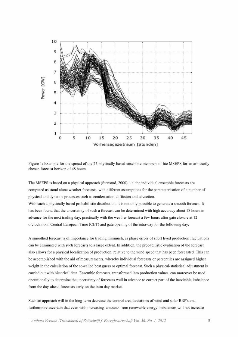
The MSEPS is based on a physical approach (Stensrud, 2000), i.e. the individual ensemble forecasts are

computed as stand alone weather forecasts, with different assumptions for the parameterisation of a number of

physical and dynamic processes such as condensation, diffusion and advection.

With such a physically based probabilistic distribution, it is not only possible to generate a smooth forecast. It

has been found that the uncertainty of such a forecast can be determined with high accuracy about 18 hours in

advance for the next trading day, practically with the weather forecast a few hours after gate closure at 12

o’clock noon Central European Time (CET) and gate opening of the intra-day for the following day.

A smoothed forecast is of importance for trading inasmuch, as phase errors of short lived production fluctuations

can be eliminated with such forecasts to a large extent. In addition, the probabilistic evaluation of the forecast

also allows for a physical localization of production, relative to the wind speed that has been forecasted. This can

be accomplished with the aid of measurements, whereby individual forecasts or percentiles are assigned higher

weight in the calculation of the so-called best guess or optimal forecast. Such a physical-statistical adjustment is

carried out with historical data. Ensemble forecasts, transformed into production values, can moreover be used

operationally to determine the uncertainty of forecasts well in advance to correct part of the inevitable imbalance

from the day-ahead forecasts early on the intra day market.

Such an approach will in the long-term decrease the control area deviations of wind and solar BRP's and

furthermore ascertain that even with increasing amounts from renewable energy imbalances will not increase


Figure 1: Example for the spread of the 75 physically based ensemble members of hte MSEPS for an arbitrarily chosen forecast horizon of 48 hours.

and/or become more expensive. In addition, this methodology is applicable not only to large amounts of wind or

solar power, i.e. for transmission system operators (TSO), but very advantageous also for small market

participants, since it allows for early balancing of errors during the night on the intra-day market without

allocating 24/7 personnel. Together with the market bonus of the renewable energy law amendment 2012 this

will not only mean more efficient operation of a larger amount of wind power units, but will also provide the

incentive for increased competition on the intra-day market. In the following we will explain a concept that

allows for this.

Description of the methodology

We propose a new methodology, whereby the correction of the forecast error for the day ahead trade begins with

the intra day trade respectively when the so called 12UTC weather forecast arrives (about 1-2 hours after

opening of the intra day market). The approach is comprised of a combination of:

a day ahead forecast (DFC)

a short term forecast for the wind energy pool (SFC)

an aggregated probabilistic uncertainty forecast for a pool/facility (UP)

From this information it is computed how much volume of the forecast error can be traded on the intra-day

market and how much and how much has to be balanced with shared balancing power. This is being done by a

sign evaluation of the expected balancing volume (AE):

AE=SFC−DFC (1)

The absolute value of the balancing volume AA is the absolute value of the difference between the day ahead

forecast (DP) and the short term forecast (KFP), from which then the probabilistic uncertainty forecast is

subtracted, i.e. the part, which can not be determined with certainty as error in the day ahead trade:

AA=∣SFC−DFC∣−UP (2)

whereby the uncertainty forecast, as defined in equation (5), is variable due to the ensemble spread that is

computed in every time step, but is always subtracted as positive value. Furthermore equation (2) is used to

control if the sign of AE in equation (1) is correct. From equations (1) and (2) we now can derive a decision table

for an automated forecast update process (FUP) (see table 1).

Tab. 1: Decision table for the forecast update process (FUP)

Case AE AA FUP a,b,c1 < 0 < 0 DP 0,0,02 < 0 > 0 KFP + UP 1,1,13 ≥ 0 > 0 KFP - UP 1,-1,14 ≥ 0 < 0 DP 0,0,0

The column with the coefficients „a,b,c“ will later on be used to determine a forecast update increment. The

principle of this decision table is illustrated in Figure 2.


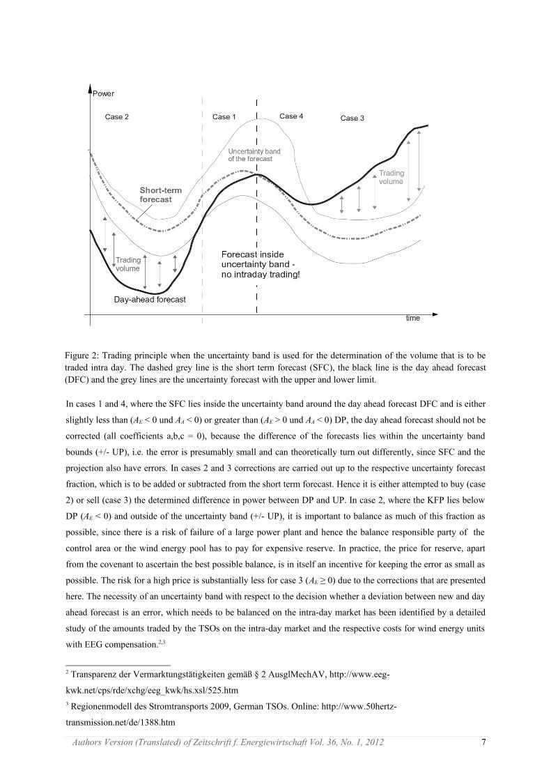
In cases 1 and 4, where the SFC lies inside the uncertainty band around the day ahead forecast DFC and is either

slightly less than (AE < 0 und AA < 0) or greater than (AE > 0 und AA < 0) DP, the day ahead forecast should not be

corrected (all coefficients a,b,c = 0), because the difference of the forecasts lies within the uncertainty band

bounds (+/- UP), i.e. the error is presumably small and can theoretically turn out differently, since SFC and the

projection also have errors. In cases 2 and 3 corrections are carried out up to the respective uncertainty forecast

fraction, which is to be added or subtracted from the short term forecast. Hence it is either attempted to buy (case

2) or sell (case 3) the determined difference in power between DP and UP. In case 2, where the KFP lies below

DP (AE < 0) and outside of the uncertainty band (+/- UP), it is important to balance as much of this fraction as

possible, since there is a risk of failure of a large power plant and hence the balance responsible party of the

control area or the wind energy pool has to pay for expensive reserve. In practice, the price for reserve, apart

from the covenant to ascertain the best possible balance, is in itself an incentive for keeping the error as small as

possible. The risk for a high price is substantially less for case 3 (AE ≥ 0) due to the corrections that are presented

here. The necessity of an uncertainty band with respect to the decision whether a deviation between new and day

ahead forecast is an error, which needs to be balanced on the intra-day market has been identified by a detailed

study of the amounts traded by the TSOs on the intra-day market and the respective costs for wind energy units

with EEG compensation.2,3

2 Transparenz der Vermarktungstätigkeiten gemäß § 2 AusglMechAV, http://www.eeg-

kwk.net/cps/rde/xchg/eeg_kwk/hs.xsl/525.htm3 Regionenmodell des Stromtransports 2009, German TSOs. Online: http://www.50hertz-

transmission.net/de/1388.htm


Figure 2: Trading principle when the uncertainty band is used for the determination of the volume that is to be traded intra day. The dashed grey line is the short term forecast (SFC), the black line is the day ahead forecast (DFC) and the grey lines are the uncertainty forecast with the upper and lower limit.

The results of this study showed, that to date a significant loss for the trade of wind energy on the intra-day

market exists. This loss is due to the fact, that it is more expensive to buy short-term additional power, than to

sell surplus wind energy on the intra-day market from a BIAS-free day-ahead forecast. When this pattern is

investigated in detail, it becomes clear, that an efficient trading system should provide neither imbalances are

trading multiple times, nor that one and the same megawatt (MW) is charged several times with reserve costs.

This can be accomplished through an approach that uses uncertainty factors – as given in Table 1 and illustrated

in Figure 2 – and by limiting the trading of imbalances to those outside an uncertainty band around the day-

ahead forecast .

The short term forecast

For the application of the approach that is presented here it is irrelevant with which procedure the short-term

forecast is determined. The forecast may be a meta forecast that stems from a series of deterministic individual

forecasts for the total production, or from an ensemble forecasting system. It is important, however, that the

forecasts cover the entire area and the entire pool, respectively, and that those are based on consistent weather

forecasts for the entire area. Otherwise there is a risk of inconsistencies and higher volatility of the errors, if for

example weather forecasts from a supplier of a certain weather service are used for one control area and

forecasts from a second supplier of another weather service are used for other control areas. In other words, the

“meta”-forecast has to be a sum of consistent forecasts for the entire pool. For our study we used a short term

forecast (SFC), which is generated with an inverted Ensemble Kalman Filter (iEnKF) approach (Möhrlen and

Jørgensen 2009), whereby the publicly available online data of the extrapolations of the individual TSO regions

are used for the adjustments of forecasts with measurements. This in turn means, that four regional extrapolation

numbers per time step are made use of to adjust the forecast for the entire area, accordingly. This procedure does

not provide an ideal forecast compared to using all available online data (so-called reference measurement

points), since the iEnKF-approach with 3-D feedback from a number of measurement locations can determine a

much more accurate actual state from many points than when using only four regional online extrapolation data

sets. Here, the authors foresee a chance in the trading of smaller pools with the bonus system of the new EEG

law amendments for 2012, as it may over time provide a substantially improved actual state of the individual

control areas and hence also a short-term forecast with higher accuracy.

The role of the uncertainty forecast in the forecast-update-process

The aggregated pool uncertainty forecast (UP) is an integral part for the forecast update process (UP) of the

proposed procedure. It dictates, which measures need to be taken and how large the amounts are that need to be

balanced at the intra-day market. The UP is independent of the day-ahead and of the short-term forecast in that

sense, that it can be generated by anyone and by any suitable method. In this study a physically based ensemble

forecast, computed with the MSEPS system that has already been explained above, has been used.

The uncertainty forecast UP has to be calibrated with historic data. Those may be forecast data that come from a

real-time system or historic data, which have been generated under real time conditions. In case that the SFC is a

meta forecast, then it is important, that the hourly forecast values are generated with the same meta forecast

combination. The first step in determining the UP is to calculate the man absolute error ( F ) of the uncorrected

short term forecast for the entire pool for one year from real time data:


N

iiF

NF

1

1(3)

where F is the absolute error, expressed as difference between short-term forecast SFC and measurements OBS

in each time step:

F i=∣SFC i−OBS i∣ (4)

Part of this error cannot be explained by the weather uncertainty. This is accounted for through the constant

uncertainty in the second term in equation (5). The remainder of the uncertainty varies with the weather. Various

tests have shown, that the uncertainty that is related to the weather can best be modeled by a physical ensemble

spread of wind production (Sw), where the correlation with the forecast error is made use of. The UP can hence

be expressed as sum of the weather dependent uncertainty and the random system uncertainty:

FFSKS

FSFSKUP www

,0,1, ~ (5)

where ~

S is the time integral of Sw and K is the correlation between the ensemble spread and the forecast error

(Sw, F). We have conducted studies that showed, that the difference between two percentiles, centered around the

median, yields good results with respect to the choice of the ensemble spread. The percentile pair with the

highest correlation (K value) is hence chosen. As an example the inter quartile range can be given: Sw = P75 –

P25. The orders or magnitude of K, Sw und F depend on one another, but those are constant for a given pool

and for a certain forecast horizon. The entire variability lies in the spread Sw. In general, K, Sw und F increase

with increasing forecast horizon, which in turn means, that the uncertainty forecast UP improves for increasing

forecast horizon for almost every pool.

However, it must be mentioned here, that the uncertainty should vary with the actual weather, i.e. it should

reflect the uncertainty that is inherent in the weather. Thereby it is important, that the uncertainty forecast stems

from a physically based approach of an ensemble system, e.g. from a multi-scheme or a multi-model approach

and not from a statistical methodology such as a variability analysis of the wind speed. The application of a

“true” ensemble forecast is in particular crucial for extreme events at the spot market, since those originate from

uncertain wind energy supply. Uncertain wind energy supply in turn arises always near fronts or low pressure

regions and in particular if those are located near or move over areas that have strong gradients of installed wind

power capacity, i.e. in areas, where production fluctuations have strong impact on the total production. Those

areas can mainly be found in coastal regions. The ensemble forecasts produce in such situations automatically

extreme spread, since the individual weather forecasts will, depending on the location of the frontal passage or

the low pressure system, produce results that will strongly differ. Now, the difference between DFC and

SFC+UP or SFC-UP can be traded according to Table 1 on the intra-day market. The resulting correction

forecast (CP) can be formulated using the three constants from Table 1:

CP=a⋅SFC+b⋅UP−c⋅DFC (6)

It will be shown that by applying this correction a refinement of the renewable energy is achieved through

discarding the part without value (the uncertain part) while retaining the part with value (the certain part).


Simulation and Analysis

A simulation for the time period of one year, from July 2010 to June 2011, has been set up in order to test the

newly developed theory. Here all wind farms in Germany have been merged, i.e. the four control zones were

considered as one zone and the balance responsible party (BRP) conducts the trading of the wind power in

accordance with the regulation of the grid control corporation (Bundesnetzagentur 2010; Zolatarev et al. 2009).

The simulation include a control area analysis for different forecast strategies for the generated wind power in

Germany. Hereby power prices on the spot market, prices on the intra-day market as well as prices for control

reserve have been calculated and analyzed accordingly. Daily day-ahead forecasts with a forecast horizon of 48

hours, 6-hourly forecast updates with short-term forecasts over 13 hours and hourly intra-day forecasts with a

forecast horizon of two hours have been generated for the time period considered here. From those forecasts 5 +

1 different scenarios have been combined, whereas the additional scenario is relevant only for the cost analysis

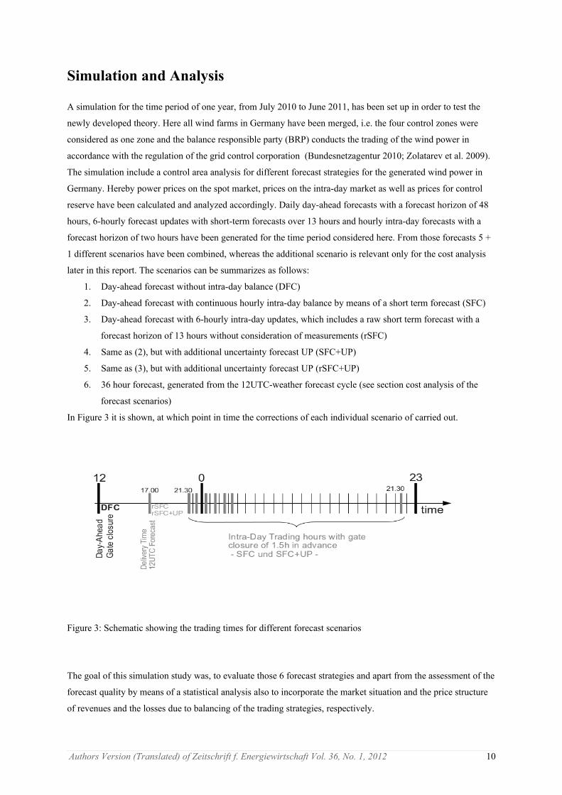
later in this report. The scenarios can be summarizes as follows:

1. Day-ahead forecast without intra-day balance (DFC)

2. Day-ahead forecast with continuous hourly intra-day balance by means of a short term forecast (SFC)

3. Day-ahead forecast with 6-hourly intra-day updates, which includes a raw short term forecast with a

forecast horizon of 13 hours without consideration of measurements (rSFC)

4. Same as (2), but with additional uncertainty forecast UP (SFC+UP)

5. Same as (3), but with additional uncertainty forecast UP (rSFC+UP)

6. 36 hour forecast, generated from the 12UTC-weather forecast cycle (see section cost analysis of the

forecast scenarios)

In Figure 3 it is shown, at which point in time the corrections of each individual scenario of carried out.

The goal of this simulation study was, to evaluate those 6 forecast strategies and apart from the assessment of the

forecast quality by means of a statistical analysis also to incorporate the market situation and the price structure

of revenues and the losses due to balancing of the trading strategies, respectively.


Figure 3: Schematic showing the trading times for different forecast scenarios

This procedure is a change in paradigm, since we accept, that it is no longer necessarily the forecast with the

smallest mean absolute or quadratic error is considered to be the best forecast, but that forecast is the best

forecast, which is capable to trade and to physically embed the fluctuating wind power and of course also solar

power in the grid in the best possible way.

To realize this, it is necessary not only to analyze the error sources, but also the consequences of forecast errors

in an economic sense. Here, we narrow our study to the analysis of losses due to balancing of forecast errors,

since this is the decisive factor for the evaluation of the economic benefit. The calculation of revenues has

deliberately been omitted, since the actual revenues depend on a multitude of factors, such as the contract

between the wind power plant owner and the trader, the actually earned prices on the spot market, etc.. Those

unknowns are for the trading strategies shown here irrelevant and were hence neglected.

It should however be mentioned, that the results may theoretically be affected by these unknown factors. For

example, if the compensation for additionally traded power on the intra-day market is high enough, so that a

BRP may bid in the wind power in the day-ahead conservatively (i.e. rather too low) in order to increase his

earnings on the intra-day market. Such action would on the other hand require that the BRP accepts to curtail

part of his pool, if there is not enough volume available on the intra-day market at time, when its required.

German TSOs are obligated to market the fluctuating wind and solar power. For a fair distribution of the task,

the so-called HoBA-principle. is being applied, which establishes a horizontal load balance, whereby the TSOs

are not assigned renewable production capacity according to its spatial distribution, but according to the

percentage of the total production capacity in their respective control zone. To accomplish this technically, an

extrapolation is carried out in each zone based on reference production plants. Those calculations are then being

interchanged amongst the TSOs. This extrapolation is based on a mere 10% of the total installed generation

capacity in Germany and is, depending on the weather situation, more or less prone to errors. On yearly average

one can assume an RMSE of 1-2% of the installed capacity and may rise up to 10% (personal communication

with Amprion GmBH). This extrapolation is used by the TSOs to generate short-term forecasts, which should

compensate the erroneous day-ahead forecast on the intra-day market. The boundary conditions for the intra-day

market are hence somewhat erroneous, which in turn can easily lead to double trading of wind power, if the total

difference between day-ahead and short term forecast is traded. In this context it is advantageous to determine

the uncertainty of the extrapolation and of the respective short-term forecast in order to circumvent, that energy

is traded multiple times.

Analysis of the forecst scenarios

The detailed analysis of the simulation results clearly showed, that the uncertainty inherent to the actual

production of wind power – and this also holds for solar power – may from case to case lead to double trading.

Not only does such double trading increase the general marketing costs, but it also increases the required balance

power, although roughly 50% of the small errors (i.e. errors < 2% of the installed capacity) benefit balancing the

system und should therefore not be balanced on the intra day market.

Balancing those small errors reduces the system security, increases the general costs of marketing and reduces

their revenues.


Firstly a statistical analysis has been carried out for the time span that was considered in this study. In Table 2

and Table 3 the RMSE and the BIAS values are summarized for different forecast types and areas.

Tab. 2 RMSE for different forecast types and areas. All values are % of inst. capacity.

Forecast type

/ area

Day-ahead

forecast00UTC

“raw”short term

forecast

iEnKFshort term

forecast

Persistence

(2 hours)

iEnKFshort-term

forecastcorrected

“raw” short-

term FCcorrected

Day-ahead

forecast12UTC

DE - 50Hertz 6.81 5.40 4.61 5.34 - - -DE – TenneT 5.39 4.14 3.42 3.96 - - -

DE – Amprion 5.13 4.36 4.03 4.03 - - -DE – EnBW 5.84 5.14 5.25 3.29 - - -

DE 4.69 3.55 2.74 3.11 3.65 4.26 4.27

Tab. 3 BIAS in different regions and forecast types. All values are % of inst. capacity.

Forecast type

/ area

Day-ahead

Forecast00UTC

“raw”Short-term

Forecast

iEnKFshort-term

forecast

Persistence

(2 hours)

iEnKFshort-term

forecastcorrected

“raw”short-

term FC corrected

Day-ahead

forecast 12UTC

DE - 50Hertz 0.57 -0.79 -0.43 0.00 - - -DE - TenneT -0.12 -1.12 -0.87 0.00 - - -

DE - Amprion 0.32 -0.94 -0.7 0.01 - - -DE - EnBW 1.75 0.33 0.55 0.00 - - -

DE 0.28 -0.87 -0.63 0.00 -0.08 0.08 -0.29

It can be seen, that those forecasts, which balance those errors only, which extend to their respective uncertainty

band, do have a smaller RMSE than the day ahead forecast, but on the other hand have a much worse RMSE

than the intra-day iEnKF forecast (SFC), the raw short-term forecast (rSFC) and the persistence of the upscaling.


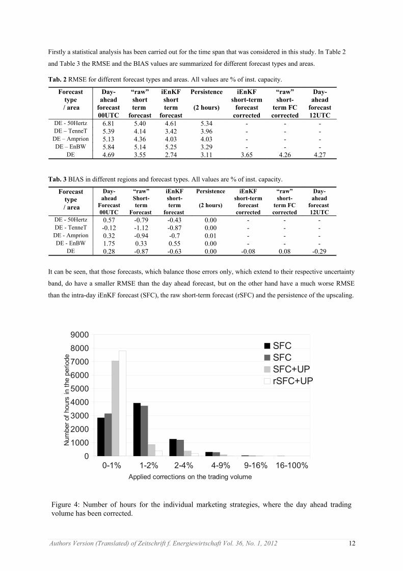
Figure 4: Number of hours for the individual marketing strategies, where the day ahead trading volume has been corrected.

0-1% 1-2% 2-4% 4-9% 9-16% 16-100%0

1000

2000

3000

4000

5000

6000

7000

8000

9000

SFCSFCSFC+UPrSFC+UP

Applied corrections on the trading volume

Num

ber

of h

o urs

in t

he p

erio

de

Only an insignificant BIAS remains for those forecasts, that have been corrected according to the uncertainty. In

Figure 4 the temporal distribution of the corrections and the magnitude of the corrections for the four intra-day

forecast scenarios that have been investigated are shown.

The difference between the distributions in the two smallest correction bins for the forecasts with and without

uncertainty forecast correction is remarkable. Furthermore a substantial reduction of the necessary corrections

for the raw short term forecast without measurements (rSFC), compared with the day ahead forecast can be seen.

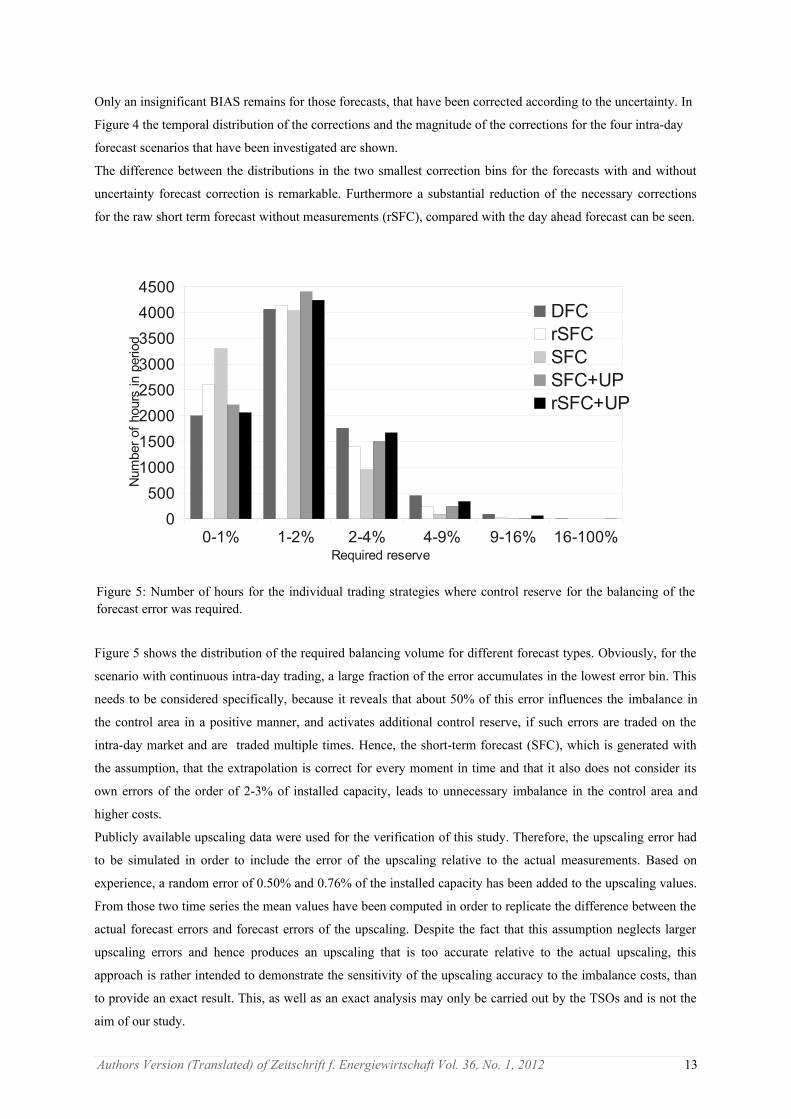
Figure 5 shows the distribution of the required balancing volume for different forecast types. Obviously, for the

scenario with continuous intra-day trading, a large fraction of the error accumulates in the lowest error bin. This

needs to be considered specifically, because it reveals that about 50% of this error influences the imbalance in

the control area in a positive manner, and activates additional control reserve, if such errors are traded on the

intra-day market and are traded multiple times. Hence, the short-term forecast (SFC), which is generated with

the assumption, that the extrapolation is correct for every moment in time and that it also does not consider its

own errors of the order of 2-3% of installed capacity, leads to unnecessary imbalance in the control area and

higher costs.

Publicly available upscaling data were used for the verification of this study. Therefore, the upscaling error had

to be simulated in order to include the error of the upscaling relative to the actual measurements. Based on

experience, a random error of 0.50% and 0.76% of the installed capacity has been added to the upscaling values.

From those two time series the mean values have been computed in order to replicate the difference between the

actual forecast errors and forecast errors of the upscaling. Despite the fact that this assumption neglects larger

upscaling errors and hence produces an upscaling that is too accurate relative to the actual upscaling, this

approach is rather intended to demonstrate the sensitivity of the upscaling accuracy to the imbalance costs, than

to provide an exact result. This, as well as an exact analysis may only be carried out by the TSOs and is not the

aim of our study.


Figure 5: Number of hours for the individual trading strategies where control reserve for the balancing of the forecast error was required.

0-1% 1-2% 2-4% 4-9% 9-16% 16-100%0

500

1000

1500

2000

2500

3000

3500

4000

4500

DFCrSFCSFCSFC+UPrSFC+UP

Required reserve

Num

ber

of h

o urs

in p

erio

d

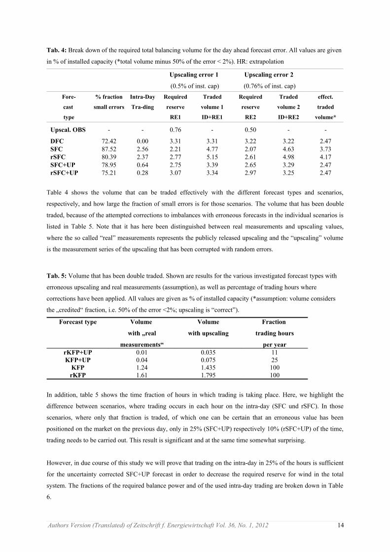
Tab. 4: Break down of the required total balancing volume for the day ahead forecast error. All values are given

in % of installed capacity (*total volume minus 50% of the error < 2%). HR: extrapolation

Upscaling error 1

(0.5% of inst. cap)

Upscaling error 2

(0.76% of inst. cap)

Fore-

cast

type

% fraction

small errors

Intra-Day

Tra-ding

Required

reserve

RE1

Traded

volume 1

ID+RE1

Required

reserve

RE2

Traded

volume 2

ID+RE2

effect.

traded

volume*

Upscal. OBS - - 0.76 - 0.50 - -

DFC 72.42 0.00 3.31 3.31 3.22 3.22 2.47SFC 87.52 2.56 2.21 4.77 2.07 4.63 3.73rSFC 80.39 2.37 2.77 5.15 2.61 4.98 4.17SFC+UP 78.95 0.64 2.75 3.39 2.65 3.29 2.47rSFC+UP 75.21 0.28 3.07 3.34 2.97 3.25 2.47

Table 4 shows the volume that can be traded effectively with the different forecast types and scenarios,

respectively, and how large the fraction of small errors is for those scenarios. The volume that has been double

traded, because of the attempted corrections to imbalances with erroneous forecasts in the individual scenarios is

listed in Table 5. Note that it has here been distinguished between real measurements and upscaling values,

where the so called “real” measurements represents the publicly released upscaling and the “upscaling” volume

is the measurement series of the upscaling that has been corrupted with random errors.

Tab. 5: Volume that has been double traded. Shown are results for the various investigated forecast types with

erroneous upscaling and real measurements (assumption), as well as percentage of trading hours where

corrections have been applied. All values are given as % of installed capacity (*assumption: volume considers

the „credited“ fraction, i.e. 50% of the error <2%; upscaling is “correct”).

Forecast type Volume

with „real

measurements“

Volume

with upscaling

Fraction

trading hours

per yearrKFP+UP 0.01 0.035 11KFP+UP 0.04 0.075 25

KFP 1.24 1.435 100rKFP 1.61 1.795 100

In addition, table 5 shows the time fraction of hours in which trading is taking place. Here, we highlight the

difference between scenarios, where trading occurs in each hour on the intra-day (SFC und rSFC). In those

scenarios, where only that fraction is traded, of which one can be certain that an erroneous value has been

positioned on the market on the previous day, only in 25% (SFC+UP) respectively 10% (rSFC+UP) of the time,

trading needs to be carried out. This result is significant and at the same time somewhat surprising.

However, in due course of this study we will prove that trading on the intra-day in 25% of the hours is sufficient

for the uncertainty corrected SFC+UP forecast in order to decrease the required reserve for wind in the total

system. The fractions of the required balance power and of the used intra-day trading are broken down in Table

6.


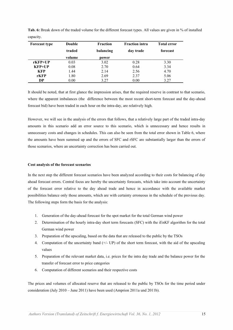
Tab. 6: Break down of the traded volume for the different forecast types. All values are given in % of installed

capacity.

Forecast type Double

traded

volume

Fraction

balancing

power

Fraction intra

day trade

Total error

forecast

rKFP+UP 0.03 3.02 0.28 3.30KFP+UP 0.08 2.70 0.64 3.34

KFP 1.44 2.14 2.56 4.70rKFP 1.80 2.69 2.37 5.06

DP 0.00 3.27 0.00 3.27

It should be noted, that at first glance the impression arises, that the required reserve in contrast to that scenario,

where the apparent imbalances (the difference between the most recent short-term forecast and the day-ahead

forecast bid) have been traded in each hour on the intra-day, are relatively high.

However, we will see in the analysis of the errors that follows, that a relatively large part of the traded intra-day

amounts in this scenario add an error source to this scenario, which is unnecessary and hence results in

unnecessary costs and changes in schedules. This can also be seen from the total error shown in Table 6, where

the amounts have been summed up and the errors of SFC and rSFC are substantially larger than the errors of

those scenarios, where an uncertainty correction has been carried out.

Cost analysis of the forecast scenarios

In the next step the different forecast scenarios have been analyzed according to their costs for balancing of day

ahead forecast errors. Central focus are hereby the uncertainty forecasts, which take into account the uncertainty

of the forecast error relative to the day ahead trade and hence in accordance with the available market

possibilities balance only those amounts, which are with certainty erroneous in the schedule of the previous day.

The following steps form the basis for the analysis:

1. Generation of the day-ahead forecast for the spot market for the total German wind power

2. Determination of the hourly intra-day short term forecasts (SFC) with the iEnKF algorithm for the total

German wind power

3. Preparation of the upscaling, based on the data that are released to the public by the TSOs

4. Computation of the uncertainty band (+/- UP) of the short term forecast, with the aid of the upscaling

values

5. Preparation of the relevant market data, i.e. prices for the intra day trade and the balance power for the

transfer of forecast error to price categories

6. Computation of different scenarios and their respective costs

The prices and volumes of allocated reserve that are released to the public by TSOs for the time period under

consideration (July 2010 – June 2011) have been used (Amprion 2011a und 2011b).


In order to account for the impact of the price for control reserve with the required amount of energy firstly a

regression analysis of the prices and the respective volumes has been carried out. A cost function should have

been the result, with which the price development for different forecast types can be simulated. However, it has

been found, that none of the state-of-the-art regression functions were capable to realistically represent the prices

as a function of volumes.

Particularly the prices for large forecast errors, which inevitably occur during strong wind periods, have been

reduced tremendously with all tested functions, so that the results were not useful any more.

Regression analysis functions are not capable to capture such sporadic and random extreme events. But precisely

those events are of utmost importance in this context. Due to those circumstances, it was decided to use the

actual prices and hence the error and the prices for reserve, respectively. In this way, the scenario “only day-

ahead forecasts” have however been underestimated. For the remaining scenarios a realistic approach is

nevertheless ensured, such that this error can be neglected.

This is especially a valid approach, because from the point of view, that the balance responsible parties have to

balance the forecast error on the intra-day as good as is feasible and not to allocate the total of the forecast error

to control reserve4.

Furthermore attention must be paid to the fact that the costs for reserve that were calculated here and the actual

balancing costs of the TSOs differ slightly, since the actual trading is based on different forecasts than those that

were used in this study. The forecasts of the TSOs are based on a meta forecast, while in this study the

production forecast was based on 75 weather forecasts. Those discrepancies may well affect the prices at the

EPEX for certain weather situations, in particular for strong wind events, since the errors will differ in their

timing and hence have a differing impact. However, the mean error is comparable and hence this consistent false

assumption of prices can be neglected.

This assumption is also equivalent to the situation of a BRP with such a small pool of marketed wind power

plants compared to the total fraction of EEG-wind, that a BRP is not in a situation to influence the prices on the

spot market.

The PHELIX market data prices of the day-ahead market at EPEX Spot have been used (EPEX 2011a). The

prices for the intra-day trading and the required reserve volume should also in this case have been determined

with the aid of a cost function, because of wind energy's impact on the prices.

If one would simply use the prices released by EPEX on the intra-day, then one would automatically prefer

certain scenarios and ignore the fact, that for large volumes there will not always be sufficient capacity available

in the intra-day. In this respect the comparison of the different scenarios would only be possible to a limited

extent. To circumvent this issue, a regression analysis of the mean prices and the related volumes on the intra-

day has been carried out. For that, a time series of prices and volumes on the intra-day of EPEX Spot for the time

span under consideration in this study (July 2010 – June 2011) has been used (EPEX 2011a).

Note, that all prices shown regarding the intra-day refer from now on to the difference to the day-ahead spot

market price, i.e. a “zero price” in the intra-day is equivalent to the spot market price of the day-ahead market. It

must hence be paid attention to the fact that all further information refers to the difference with the day-ahead

spot market price and are not absolute prices.

4 http://www.amprion.net/bilanzkreisfuehrung#


The analysis of the regression coefficients revealed, that the regression can not reflect zero prices (spot market

price = intra-day price) appropriately and that this would undermine the price function, since the number of zero

prices is for one to large and secondly is an important price category in the cost analysis.

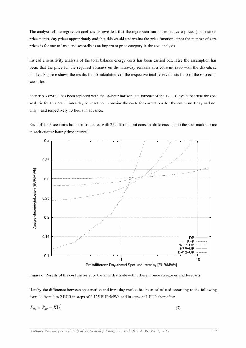
Instead a sensitivity analysis of the total balance energy costs has been carried out. Here the assumption has

been, that the price for the required volumes on the intra-day remains at a constant ratio with the day-ahead

market. Figure 6 shows the results for 15 calculations of the respective total reserve costs for 5 of the 6 forecast

scenarios.

Scenario 3 (rSFC) has been replaced with the 36-hour horizon late forecast of the 12UTC cycle, because the cost

analysis for this “raw” intra-day forecast now contains the costs for corrections for the entire next day and not

only 7 and respectively 13 hours in advance.

Each of the 5 scenarios has been computed with 25 different, but constant differences up to the spot market price

in each quarter hourly time interval.

Figure 6: Results of the cost analysis for the intra day trade with different price categories and forecasts.

Hereby the difference between spot market and intra-day market has been calculated according to the following

formula from 0 to 2 EUR in steps of 0.125 EUR/MWh and in steps of 1 EUR thereafter:

iKPP SPID (7)


where PID is the intra-day price, PSP is the spot market price and K(i) runs from 0...13 EUR in steps of 0,125 and

1,0 EUR/MWh, respectively. K(i) is positive, if power amounts are sold and negative, is power amounts have to

be bought.

In addition the reserve costs for the trading on the day-ahead market without correction are shown in Figure 6.

Figure 6 may give the impression that the UP forecast is substantially more accurate than the KFP forecast.

Closer examination reveals however, that:

for permanent hourly intra-day trading at the 90min gate closure, relatively large balance volumes are

required and hence there is a risk, that not enough volume is available on the market at this time.

one can allow for a larger price difference between DFC and SFC, if the main portion of the expected error is

already placed and traded on the intra-day one day in advance.

the intra-day price analysis showed, that a price difference of less than 1.5 EUR/MWh with the PHELIX spot

market price on the intra-day is difficult to achieve, in particular shortly before gate closure.

the probabilistic uncertainty forecast can almost at all times be realized, since a major part of the corrections

are traded on the previous day and only a small remainder has to be traded shortly before gate closure. For

the latter, a larger price difference is hence acceptable.

through the uncertainty forecast a BRP can take advantage of the possibility to use the price level up to the

forecasted UP volume with different trading types on the intra-day market – already 12 to 18 hours before

gate closure.

Furthermore, it becomes clear, that each scenario within a certain loss margin has advantages when compared

with other scenarios. The 2-hour short-term forecast is suited best for minor losses at a spot market price up to

1.3 EUR. From 1.3 to 3.0 EUR loss, the 2-hour short-term forecast under consideration of the uncertainty

correction should be applied. From 3.0 to 13.0 EUR loss only an intra-day update in the late afternoon of the

previous day is beneficial. For losses beyond 13.0 EUR only that volume should be auctioned on the intra-day

market, from which the BRP can be certain, that this volume is missing or will be superfluous, since the loss will

be very high.

Uncertainties have to be allocated to an automatic imbalance regulation mechanism in this case. Generally,

Figure 6 shows, that trading of forecast errors of the day-ahead needs to be carried out intelligently and with

caution.

Furthermore it can be seen, that no appropriate statistical method exists for this multifaceted issue, but that a

flexible use of different trading methods and trading types leads to the best result. This does not imply that

automated solutions are unfeasible, but rather that their complexity increases. With the uncertainty forecast

strategy, we however aim at introducing a methodology, which allows for automation of those complex links.

We hope that this will provide an impetus for more dynamic trading.


As an example where we now consider the findings of this study and look at Figure 6, we can derive the

following exemplary trading strategy at time 17:30:

Calculation of the difference between DFC at 00 UTC and DFC at 12 UTC

Calculation of the new uncertainty bands and balancing volumes

Establish price levels according to the newly released spot prices for the next day and setting up trading

volumes for the intra-day at equal or different price levels up to the uncertainty band limit

Positioning of the volume according to the calculated prices that is to be traded on the intra-day market

Calculation of the residual volume from the uncertainty band for the comparison with the new forecasts until

compliance is reached

Trading of the residual volume shortly before gate closure

When setting up the intra-day trading volume one can make use of different trading tools inside and outside of

the “order books”, such as “limit orders” and “market sweep orders”, etc. (EPEX 2011b).

Discussion

The overall goal of this work was to clarify the important problem, as to what extent intra-day trading is required

in addition to the day-ahead spot market auction and technically useful for efficient trading and balancing of

wind energy. The benefit of a trading strategy has been investigated, where the intra-day trading is not only

carried out 2h before gate closure, but already at or shortly after opening of the intra-day market in the afternoon

of the previous day.

For this purpose forecasts have been generated that are available for the next day already one hour in winter and

two hours in summer after opening of the intra-day market (15:00 CET of the previous day) and that are based

on a new weather forecast of the so-called 12UTC cycle (the day-ahead trade is generally based on the so called

00UTC forecasts).

The most important value of this day-ahead forecast lies in the correction that then can be made much earlier

instead of in the last moment. This is particularly important during extreme situations. One can hence expect to

have a substantially lower loss relative to the spot market price on the previous day. Hereby it is important to

understand, that this 12UTC forecast is from a meteorological point of view the qualitatively best weather

forecast for Western Europe, because for this forecast the largest number of measurements from transatlantic

flights are available. Furthermore, a forecast is made use of for the next day with a forecast horizon that is 12

hours shorter and therefore with a mean improvement in quality of about 10% of installed capacity, measured in

RMSE.

Figure 7 shows an example of the development of the uncertainty distribution of a forecast evolution over the

course of six days. However, not a forecast with a forecast horizon of six days has been computed, but instead

from 24 different forecast runs we have extracted those forecasts, which exhibit the same point in time for which

the forecast is valid (here: 2011/09/20-03:00 UTC). Therefore, forecasts with 144, 136, 130...24, 18, 12, 6 hour

forecast horizon are combined in one graph.


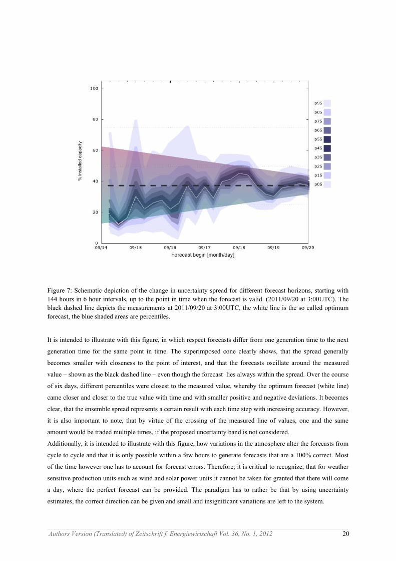
It is intended to illustrate with this figure, in which respect forecasts differ from one generation time to the next

generation time for the same point in time. The superimposed cone clearly shows, that the spread generally

becomes smaller with closeness to the point of interest, and that the forecasts oscillate around the measured

value – shown as the black dashed line – even though the forecast lies always within the spread. Over the course

of six days, different percentiles were closest to the measured value, whereby the optimum forecast (white line)

came closer and closer to the true value with time and with smaller positive and negative deviations. It becomes

clear, that the ensemble spread represents a certain result with each time step with increasing accuracy. However,

it is also important to note, that by virtue of the crossing of the measured line of values, one and the same

amount would be traded multiple times, if the proposed uncertainty band is not considered.

Additionally, it is intended to illustrate with this figure, how variations in the atmosphere alter the forecasts from

cycle to cycle and that it is only possible within a few hours to generate forecasts that are a 100% correct. Most

of the time however one has to account for forecast errors. Therefore, it is critical to recognize, that for weather

sensitive production units such as wind and solar power units it cannot be taken for granted that there will come

a day, where the perfect forecast can be provided. The paradigm has to rather be that by using uncertainty

estimates, the correct direction can be given and small and insignificant variations are left to the system.


Figure 7: Schematic depiction of the change in uncertainty spread for different forecast horizons, starting with 144 hours in 6 hour intervals, up to the point in time when the forecast is valid. (2011/09/20 at 3:00UTC). The black dashed line depicts the measurements at 2011/09/20 at 3:00UTC, the white line is the so called optimum forecast, the blue shaded areas are percentiles.

It is important in this context to understand, which fraction of this variability are traded and which fraction

should be left to the system, in order to accomplish both, a well functioning power network and to achieve a

lucrative power trading with fluctuating renewable energies.

Apart from the meteorological aspects it also can be expected, that an expansion of this preliminary trading

practice will lead to the possibility for participation in the intra-day for conventional power plants with longer

start-up periods, which did not receive contracts in the day-ahead spot market. This will have positive impact on

prices and the environment as they may be in a position to reduce start-up fuels and costs. It can certainly be

assumed that bidding in imbalances into the intra-day market at an early stage will provide the opportunity to

participation for a higher number of stakeholders. This in turn increases the available volume and competition is

fostered.

Furthermore, an alternative has been investigated in this study, where an hourly bid based on a 2-hour forecast, is

put into the market. Those forecasts are on the one hand more accurate, but on the other hand short lived and

bring in only little market volume at times. Due to the relatively long and expensive start up phase of many

conventional power plants, only one possibility emerges as being a cost efficient trading possibility for this

forecast horizon: the exchange of the forecast imbalance with other fluctuating production units. It may also be

feasible to offset imbalances competitive through foreseeable consumption of cooling units or special production

units. Yet this possibility of an imbalance offset is not always available and it also requires personnel, which

often is not at ones disposal, particularly not 24/7. As a consequence, the risk for individual large errors in

extreme weather situations and hence extreme balancing costs remains, which is unfavorable for small pools and

may easily lead to financial problems.

Conclusions and Outlook

The results shown here are based on publicly released data and are applicable to all of Germany. The usage of

the results is of value for both, the large pools of the TSOs, smaller fractions of the total number of wind energy

units and furthermore for special renewable energy pools. The forecast error will in fact be higher for small

pools.

It can however be expected, that the methodologies and results can also be applied to pools of 5 and more wind

farms of equal size and distance to each other, since smoothing effects of wind speed changes of high frequency

in the atmosphere will only be in effect from a certain number of wind farms (Vincent et al. 2010; 2011). For a

smaller number of wind farms there is a risk that the high frequency oscillations are in phase and hence the

predictability is reduced substantially. It must of course be considered, that the distribution of the wind farms

affects the accuracy for any forecast horizon.

In this study the combined loss from intra-day trading and balancing costs has been simulated with 15 minute

standardized reserve prices (reBAP). For this to be realistic, four different trading scenarios with a fixed loss

ratio from the intra-day market to the day-ahead market as well as actual balancing costs have been set up. In

addition a reference scenario has been set up, where only the day-ahead market has been considered.


It has been assumed, that the forecast does not influence the reBAP price. This approach is equivalent to a

situation, where the BRP is responsible for a small part of the total wind energy production only, such that even

the maximum imbalance of this pool would influence the price.

The results show, that an hourly execution of an automated algorithm, based on a short term forecast under

consideration of uncertainty, i.e. an uncertainty band, is very promising. The residual volume that the algorithm

determines is merely a last correction for the late afternoon forecast of the previous day, which in turn is already

a correction of the contracted capacity on the day-ahead spot market auction. However, the calculation of the

expected additional hourly short- term trading shortly before gate closure of a given contract hour reveals, that

on average only every fourth hour, i.e. only in 25% of the time a second correction is necessary, as long as

sufficient volume for the desired price for the early correction of the previous day is available on the market. The

more wind energy is integrated in the market, the more likely is a compensation of the imbalance with little loss.

The internal balance between fluctuating renewable energy production units does not change the total balancing

requirement, but it increases the production reliability and this in turn results in an indirect benefit for the total

system.

On the other hand, the opposite situation may also occur, precisely if the direct marketing practice leads to a split

up of wind energy production units into many small pools and hence to a “life on its own” of the pool balance

responsible parties (BRPs). This is when the individual BRP does not count on being able to regulate all

imbalances in time and without losses in the intraday. In such a case the situation may arise, that participants,

which are responsible for balancing wind energy, curtail their contracted wind energy production units, in order

to avoid a large imbalance with extreme prices, if extreme costs for a day-ahead forecasted overproduction is

expected. Therefore, an imbalance may occur all of a sudden in the total system with opposite sign, since those

participants, which predicted a production that was too low, cannot compensate their imbalance anymore. Such a

risk for an asymmetry of fluctuating renewable energy production units to half controlled units because of fear of

extreme balance costs would be highly counterproductive for a functional power network with high percentage

of fluctuating production units.

For that reason it is crucial and of general interest, that all market participants are at any given time in a position

to balance their forecasted production, based on the most recent forecast before market closure. This in turn

means, that balancing area imbalances and pool imbalances should always and any one be balanced via market

mechanisms, in order to guarantee sufficient volume and competitive prices. This task must not only be practiced

by the TSOs, which are responsible for that. Through timely balancing a reduction of losses is achieved.

Conventional power plants should accordingly aim for reacting to this situation, whereby the chances for a

production or consumption that can be planned is substantially higher 8-10 hours in advance, if the trading

transaction is offered for the or close to the spot market price. The more wind energy producers and other

production units implement this procedure in practice, the lower are balancing costs and the higher the efficient

integration of renewable energy and its expansion.

With the forecasting technique described here it has been shown, that by using the newly created possibilities for

direct marketing in the amendment to the renewable energy law 2012, the trading practice can be carried out

more dynamic and at the same time be beneficial for all market participants.


Literature

50Hertz (2009) Regionenmodell des Stromtransports 2009, German TSOs. http://www.50hertz-

transmission.net/de/1388.htm

Amprion (2011a) Ausgleichsenergieabrechnung gegenüber der Bilanzkreisverantwortlichen.

http://www.amprion.net/ausgleichsenergiepreis#

Amprion (2011b) Am Intra-Day-Markt beschaffte bzw. veräußerte Strommenge.

http://www.amprion.net/bilanzkreis-eeg#

BMJ (2002) Kraft-Wärme-Kopplungsgesetz vom 19. März 2002 (BGBl. I S. 1092), das zuletzt durch Artikel 11

des Gesetzes vom 28. Juli 2011 (BGBl. I S. 1634) geändert worden ist, http://www.gesetze-im-

internet.de/kwkg_2002/index.html

BMU (2011) Gesetz zur Neuregelung des Rechtsrahmens für die Förderung der Stromerzeugung aus

erneuerbaren Energien. http://www.bmu.de/erneuerbare_energien/downloads/doc/47585.php

BMU (2008) Gesetz für den Vorrang Erneuerbarer Energien (Erneuerbare-Energien-Gesetz – EEG).

http://www.bmu.de/erneuerbare_energien/downloads/doc/40508.php

Brankovic C, Palmer TN, Molteni F, Tibaldi S, Cubasch U (1990) Extended-range predictions with ECMWF

models: time-lagged ensemble forecasting, Q. J. R. Meteorol. Soc., 116: 867-912

Bundesnetzagentur für Elektrizität, Gas, Telekommunikation, Post u.Eisenbahnen (2010) Beschluss BK6-08-111

EEG-KWK (JAHR)Transparenz der Vermarktungstätigkeiten gemäß § 2 AusglMechAV, http://www.eeg-

kwk.net/cps/rde/xchg/eeg_kwk/hs.xsl/525.htm

EPEX SPOT (2011a) http://www.epexspot.com/de/presse/nachrichten/details/news/Konferenz_EPEX_SPOT_

BNetzA_zu_Erneuerbaren_Energien

EPEXSPOT (2011b) EPEX Spot Operational Rules, 08-08-2011

Jørgensen JU, Möhrlen C (2011) Increasing the competition on reserve for balancing wind power with the help

of ensemble forecasts, Proceedings 10th International Workshop on Large-Scale Integration of Wind Power into

Power Systems as well as on Transmission Networks for Offshore Wind Power Plants, Aarhus, Denmark

Lang S, Möhrlen C, Jørgensen J, ÓGallachóir B, McKeogh E (2006) Application of a multi-scheme ensemble

prediction system for wind power forecasting in Ireland and comparison with validation results from Denmark,

Scientific Proceedings European Wind Energy Conference, Greece


Möhrlen C (2004) Uncertainty in Wind Energy Forecasting, Thesis (PhD) Department of Civil and

Environmental Engineering, University College Cork, Ireland, DP2004 MOHR

Möhrlen C, Jørgensen JU (2006) Forecasting wind power in high wind penetration markets using multi-scheme

ensemble prediction methods, Proceedings German Wind Energy Conference DEWEK, Bremen, Germany

Möhrlen C, Jørgensen JU, Pinson P, Madsen H, Runge Kristoffersen J, HRENSEMBLEHR - HIGH

RESOLUTION ENSEMBLE FOR HORNS REV, Proceedings European Offshore Wind Energy Conference,

Berlin, 2007.

Möhrlen C, Jørgensen JU (2009) A new algorithm for Upscaling and Short-term forecasting of wind power using

Ensemble forecasts, Proceedings 8th Int. Workshop on Large-Scale Integr. of Wind Power

Molteni F, Buizza R, Palmer TN, Petrollagis T (1996) The ECMWF Ensemble Prediction System: Methodology

and Validation, Q.J. R. Meteorol. Soc., 122:73-119

Nanahara T, Asari M, Maejima T, Sato T, Yamaguchi K, Shibata M (2004) Smoothing effects of distributed

wind turbines. Part 2. Coherence among power output of distant wind turbines. Wind Energy, 7:75–85

Palmer TN, Molteni F, Mureau R, Buizza R, Chapelet P, Tribbia J (1993) Ensemble Prediction, ECMWF

seminar proceedings „Validation of models over Europe“, Vol 1, ECMWF, Shinfield Park, Reading, UK

Stensrud, DJ, Bao, JW, Warner, TT (2000) Using Initial Condition and Model Physics Perturbations in Short-

Range Ensemble Simulations of Mesoscale Convective Systems , Month. Weath. Rev., 128: 2077-2107

Toth Z, Kalnay E (1993) Ensemble forecasting at NMC: the generation of perturbations. Bull. Am. Meteorol.

Soc., 74: 2317-2330

Tastu J, Pinson P, Kotwa E, Madsen H, Nielsen HA (2011), Spatio-temporal analysis and modeling of short-term

wind power forecast errors. Wind Energy, 14:43–60.

Vincent C, Giebel G, Pinson P, Madsen, H (2010) Resolving nonstationary spectral information in wind speed

time series using the Hilbert–Huang Transform. J. Appl. Meteor. Climatol., 49:253–267

Vincent, C. L., Pinson, P. and Giebela, G. (2011), Wind fluctuations over the North Sea. International Journal of

Climatology, 31: 1584–1595

Zolotarev P, Treuer M, Weißbach T, Gökeler M (2009) Netzregelverbund, Koordinierter Onsets von

Sekundärregelleistung. VDI-Berichte 2080, VDI-Verlag GmbH, ISBN:9783180920801


investigation of various trading strategies for wind...

Documents