investigation of three-dimensional e ects on a … of three-dimensional e ects on a cavitating ......
TRANSCRIPT

Investigation of three-dimensional effects on a cavitating
Venturi flow
Jean Decaix, Eric Goncalves da Silva
To cite this version:
Jean Decaix, Eric Goncalves da Silva. Investigation of three-dimensional effects on a cavitatingVenturi flow. International Journal of Heat and Fluid Flow, Elsevier, 2013, 44, pp.576-595.<10.1016/j.ijheatfluidflow.2013.08.013>. <hal-00866577>
HAL Id: hal-00866577
https://hal.archives-ouvertes.fr/hal-00866577
Submitted on 26 Sep 2013
HAL is a multi-disciplinary open accessarchive for the deposit and dissemination of sci-entific research documents, whether they are pub-lished or not. The documents may come fromteaching and research institutions in France orabroad, or from public or private research centers.
L’archive ouverte pluridisciplinaire HAL, estdestinee au depot et a la diffusion de documentsscientifiques de niveau recherche, publies ou non,emanant des etablissements d’enseignement et derecherche francais ou etrangers, des laboratoirespublics ou prives.

Investigation of three-dimensional effects on a cavitating
Venturi flow
Jean Decaix∗, Eric Goncalves
LEGI-Grenoble INP, 1025 rue de la Piscine, 38400 St Martin d’Heres, France
Abstract
A numerical investigation of the behaviour of a cavitation pocket developing along a
Venturi geometry has been performed using a compressible one-fluid hybrid RANS/LES
solver. The interplay between turbulence and cavitation regarding the unsteadiness
and structure of the flow is complex and not well understood. This constitutes a
determinant point to accurately simulate the dynamic of sheet cavities. Various tur-
bulent approaches are tested: a new Scale-Adaptive model and the Detached Eddy
Simulation. 2D and 3D simulations are compared with the experimental data. An
oblique mode of the sheet is put in evidence.
Keywords: Cavitation, Homogeneous model, Scale-Adaptive model, 3D effects,
Instabilities
∗Corresponding author.Email address: [email protected] (Jean Decaix )
Preprint submitted to Elsevier July 2, 2013

Nomenclature
Abbreviation
CFD Computational Fluid Dynamic
CFL Courant-Friedrichs-Lewy num-
ber
DES Detached Eddy Simulation
DFT Direct Fourier Transform
EOS Equation Of State
LES Large Eddy Simulation
PANS Partial Average Navier-Stokes
RANS Reynolds-Average Navier-
Stokes
RMS Root Mean Square
SA Spalart and Allmaras turbulence
model
SAS Scale-Adaptive Simulation
TBLE Turbulent Boundary Layer
Equations
Greek symbols
α Void fraction
ǫ Turbulent dissipation rate
κ Von Karman constant
λ Mixture thermal conductivity
λt Mixture turbulent thermal conduc-
tivity
µ Mixture dynamic viscosity
µt Mixture dynamic eddy viscosity
ρ Mixture density
ρsatL Density of liquid at saturation
ρsatV Density of vapour at saturation
σ cavitation parameter
τ Mixture total stress tensor
ν Pseudo eddy-viscosity
Latin symbols
Cp Heat capacity at constant pressure
cbaro Minimum speed of sound in the
mixture
CDES Constant of the DES model
2

d New distance of the DES model
d Distance to the nearest wall
e Mixture internal energy
Fc Convective flux density
Fv Viscous flux density
k Mixture turbulent kinetic energy
ℓ Integral turbulence length scale
Lvk Von Karman length scale
P Mixture pressure
Pk Turbulent production term
Pr Prandtl number
Prt Turbulent Prandtl number
Q Mixture total heat flux
Re Reynolds number
S Source term
Sij Stress tensor
T Temperature
u+ Non dimensional wall velocity
ui Mass velocity vector
Uτ Friction velocity
w Vector of conservative variables
y+ Non dimensional wall distance
Subscript
inlet Inlet value
k k-phase
ref Reference value
w Wall value
Superscript
t Turbulent part
v Viscous part
3

1. Introduction
Cavitation is a significant engineering phenomenon that occurs in fluid machin-
ery, fuel injectors, marine propellers, nozzles, underwater bodies, etc. In most cases,
cavitation is an undesirable phenomenon, significantly degrading performance, re-
sulting in reduced flow rates, lower pressure increases in pumps, load asymmetry,
vibrations, noise and erosion. Such flows are characterized by important variations
of the local Mach number (due to the drastic diminution of the speed of sound in the
mixture), large density ratio between the liquid and the vapour phases, small-scale
turbulence interactions and non equilibrium thermodynamic states.
A considerable effort has been realized to understand the fundamental physics of
cavitation phenomena concerning the dynamics of both sheet and cloud cavitation.
Cavitation sheets that appear on solid bodies are characterized by a closure region
which always fluctuates, with the presence of a re-entrant jet. This jet is mainly
composed of liquid which penetrates the attached cavity from downstream and flows
upstream along the solid surface. Partial cavity can be classified as either closed or
open attached cavity, depending on the flow in the cavity closure region. A closed
partial cavity has a relatively stable cavity length and a cavity closure that is rel-
atively free of bubbles. An open cavity is typically frothy in appearance, and has
a periodically varying length that is associated with the shedding of vapour clouds
[1]. Both types of cavities have been studied, experimentally and numerically, to
describe and investigate the transition between stable and unstable behaviour, the
development of the re-entrant jet, the interaction with the turbulent boundary layer,
and the mechanism of cloud cavitation generation [2, 3, 4, 5].
Observations on hydrofoils with high-speed motion pictures put in evidence the three-
4

dimensional structures associated with the phenomena. The re-entrant jet does not
progress uniformly toward the leading edge according to the spanwise location, and
the jet component normal to the closure line is reflected inward [6]. Studies of the
spanwise effect through the sweep angle concluded the re-entrant jet was directed
into the cavity allowing for a steady sheet which only sheds cavitating clouds at the
far downstream edge [7]. To distinguish between various directions of the re-entrant
flow, the term side-entrant jet was introduced. This term refers to the part of the jet
that has a strong spanwise velocity component directed into the cavity originating
from the sides. The term re-entrant jet is reserved for the flow originating from the
part of the cavity where the closure is more or less perpendicular to the incoming
flow and is thus mainly directed upstream. The shape of the closure region of the
cavity sheet governs the direction of the re-entrant and side-entrant jets. Both jets
may form an equally important source for the shedding [8]. The spanwise variation
in the cavity and its evolution leads to important variations in the thickness and the
void fraction of the sheet. The cloud cavitation structures generated are also fully
3D. The 3D shedding mechanism studied on a twisted hydrofoil marked differences
with the 2D shedding, and included secondary instabilities caused by side-entry [8].
Recently, an experimental analysis of a pulsating cavitation sheet made appear the
presence of a bifurcation of the cavitation sheet behaviours [9]. To put in evidence
this bifurcation, the authors applied the Proper Orthogonal Decomposition (POD)
and the Dynamic Mode Decomposition (DMD), which allowed to give the energetic
spectrum of the structures and the associated frequency. It seemed that when the
cloud shedding mechanism was driven by a shock wave, a low frequency associated
with spanwise structures is observed.
Besides these experimental investigations, numerical simulations were performed
5

to investigate such 3D unsteady cavitating flows on hydrofoils and venturis, based on
mixture homogeneous models (one-fluid methods). Various assumptions were done
on the viscous effects and the turbulence modelling. Inviscid compressible codes have
been developed to simulate the 3D twisted hydrofoil, with a special emphasis on the
detection of shock formation and propagation [10], or a study of the dynamics of
the phenomena [11]. To investigate the cavitation-turbulence interaction occurring
at small scales and the mechanism that generates the large-scale vortex structure,
3D turbulent codes have been developed. Different approaches for the turbulence
modelling have been investigated in order to capture the finer-scale dynamics. First
computations were performed solving the unsteady Reynolds-Averaged Navier-Stokes
(URANS) equations coupled with transport-equation turbulence models. Recently,
URANS computations of the 3D twisted hydrofoil showed the ability of such a com-
putation to capture the large scales of the cavitation sheet [12]. As the URANS
approach did not fully account for the turbulent-cavitation interactions, Large Eddy
Simulations (LES) were tested on both hydrofoil and Venturi geometries [13, 14].
Yet, due to high Reynolds number flows and the significant cost in the computa-
tional requirements, simulations were performed on coarse grids which leading to
under-resolved simulations. To overcome the high computational cost of a wall re-
solved LES, a wall model based on the logarithmic law of the wall was introduced in
an implicit LES solver [15, 16]. Validations on 3D cavitating cases clearly exhibited
secondary cavitating vortices in spite of the small spanwise extension. Another strat-
egy proposed by Spalart, referred to as Detached-Eddy Simulation (DES), enables
to simulate smaller scales with a minimal computational cost [17]. First cavitating
simulations were proposed for a massively separated hydrofoil [18], but results were
far from statistically stationary. Other simulations were performed on ventilated
bodies and an ogive [19] where DES appeared to yield more accurate flow mod-
6

elling. A comparison with URANS, DES and ILES approach was proposed on the
twisted cavitating foil [20]. The major mechanisms governing the shedding dynam-
ics were well captured by simulations except for the URANS approach. Recently,
the Partial-Averaged Navier-Stokes (PANS) approach based on a k − ε turbulence
model, initially developed for aerodynamic flows, was tested for a cavitating flow
around a marine propeller [21] and the twisted hydrofoil [22]. This approach aims
at resolving a substantial part of the turbulent fluctuations but does not contain an
explicit dependency on the computational grid as LES. It involves the ratio of the
unresolved-to-total kinetic energy fk and the ratio of the unresolved-to-total dissi-
pation rate fε in the model constants. The user decides a priori how much of the
kinetic energy and dissipation rate is to be modelled.
In previous work, an in-house finite-volume code solving the URANS compress-
ible equations was developed with a mixture homogeneous approach. The cavitation
phenomenon was modelled by a barotropic liquid-vapour mixture equation of state
(EOS). Preliminary 2D computations were performed to assess the numerical as-
pects, thermodynamic constraints on the EOS and the influence of various transport-
equation turbulence models [23, 24]. Recently, an hybrid RANS/LES model able
to adjust the level of turbulent eddy viscosity was developed and validated on 2D
Venturi flows [25]. Such a strategy called Scale-Adaptive Simulation (SAS) was in-
troduced by Menter and Egorov (see [26] for a review of the SAS model). From
their work, we derived two SAS turbulence models based on one- and two-equation
models. As the PANS approach, Scale-Adaptive models do not imply explicitly a
dependence on the grid. To compare these models with other hybrid RANS/LES
models, computations are performed with the DES approach of Spalart. We per-
formed 2D and 3D computations, which show the advantage of hybrid RANS/LES
7

turbulence models compared with standard turbulence models. Analyses have been
conducted with a special emphasis on the 3D effects. Our goals in this study are:
• To test a new formulation of a scale-adaptive model for cavitating flows and to
investigate the behaviour of the proposed model on unsteady cavitating flows.
• To study 3D effects on a Venturi geometry by comparing 2D and 3D simula-
tions.
• To compare SAS and DES for the simulation of cavitating flows.
This paper is organized as follows. We present first the governing equations,
including the physical models, followed by an overview of the numerical methods
adopted. The Venturi configuration and the associated numerical parameters are
then presented. 2D and 3D simulations are described and compared with experi-
mental data. A deeper analysis of the 3D flow simulated with the Scale-adaptive
model is proposed and discussed. The last part deals with conclusions and future
investigations.
2. Models, equations and numerics
The numerical simulations are carried out using an in-house CFD code solving
the one-fluid compressible hybrid RANS/LES system.
2.1. The homogeneous approach
The homogeneous mixture approach is used to model two-phase flows. The phases
are assumed to be sufficiently well mixed and the disperse particle size are sufficiently
small thereby eliminating any significant relative motion. The phases are strongly
coupled and moving at the same velocity. In addition, the phases are assumed to
8

be in thermal and mechanical equilibrium: they share the same temperature T and
the same pressure P . The evolution of the two-phase flow can be described by the
conservation laws that employ the representative flow properties as unknowns just
as in a single-phase problem. We introduce αk the void fraction or the averaged
fraction of presence of phase k. The density ρ, the center of mass velocity u and the
internal energy e for the mixture are defined by [27]:
ρ =∑
k
αkρk (1)
ρui =∑
k
αkρkuk,i (2)
ρe =∑
k
αkρkek (3)
To close the system, an equation of state (EOS) and a thermal relation are neces-
sary to link the pressure and the temperature to the internal energy and the density.
2.2. The cavitation model
To link the pressure to the thermodynamic variables, the stiffened gas EOS is
used for pure phases. In the mixture, a barotropic law proposed by Delannoy [28] is
considered.
This law is characterized by its maximum slope 1/c2baro. The quantity cbaro is an
adjustable parameter of the model, which can be interpreted as the minimum speed
of sound in the mixture.
When the pressure is between Pvap +∆P and Pvap −∆P , the following relationship
applies:
P (α) = Pvap +
(ρsatL − ρsatV
2
)c2baro Arcsin (1− 2α) (4)
where ∆P represents the pressure range of the law and, for a void ratio value of
0.5, the pressure is equal to the saturation pressure Pvap. This law introduces a small
9

non-equilibrium effect on the pressure. Moreover, we assume that thermodynamic
effects on the cavitation are negligible.
The hyperbolicity and convexity of the EOS have been demonstrated for the
inviscid system [23]. The influence of cbaro has been studied in previous work. In the
present paper, the value of cbaro is set to 0.47 m/s, corresponding to a pressure range
of ∆P = 175 Pa.
2.3. Hybrid RANS/LES turbulence modelling
For turbulent computations, the Reynolds-Averaged Navier-Stokes equations are
used in an hybrid RANS/LES framework, coupled with two-equation turbulence
models. For low Mach number applications, an inviscid preconditioning method
is necessary [29, 30], based on the modification of the derivative term by a pre-
multiplication with a suitable preconditioning matrix Pc. These equations can be
expressed as:
P−1c
∂w
∂t+ div (Fc − Fv) = S (5)
w =
ρ
ρV
ρE
ρk
ρΨ
; Fc =
ρV
ρV ⊗ V + pI
(ρE + p)V
ρkV
ρΨV
; Fv =
0
τ v + τ t
(τ v + τ t).V −Qv −Qt
(µ+ µt/σk) grad k
(µ+ µt/σΨ) gradΨ
where w denotes the conservative variables, Fc and Fv the convective and viscous
flux densities and S the source terms, which concern only the transport equations.
k is the mixture turbulent kinetic energy and Ψ is a mixture turbulent variable.
10

The exact expression of the eddy-viscosity µt and the source terms depends on the
turbulence model as well as constants σk and σΨ.
The total stress tensor τ is evaluated using the Stokes hypothesis, Newton’s law and
the Boussinesq assumption. The total heat flux vector Q is obtained from the Fourier
law involving a turbulent thermal conductivity λt with the constant Prandtl number
hypothesis.
τ = τ v + τ t = (µ+ µt)
[( gradV + ( gradV )t)−
2
3( divV )I
]−
2
3ρkI
Q = Qv +Qt = − (λ+ λt) gradT with λt =µtCp
Prt
(6)
In pure liquid, the viscosity µ is determined by an exponential law and, in pure
vapour, the viscosity follows the Sutherland law. The mixture viscosity is defined
as the arithmetic mean of the liquid and vapour viscosities (fluctuations of viscosity
are neglected) [27]:
µL(T ) = µ0L exp (B/T ) (7)
µV (T ) = µ0V
√T
293
1 + TS/293
1 + TS/T(8)
µ(T, α) = αµV (T ) + (1− α)µL(T ) (9)
where µ0L , µ0V , B and TS are constants.
The mixture thermal conductivity λ is also defined as the arithmetic mean of the
liquid and vapour values:
λ(α) = αµVCpV
PrV
+ (1− α)µLCpL
PrL
(10)
The turbulent Prandtl number Prt is set to 1.
11

2.4. The turbulence modelling
Computations of cavitating flows with standard turbulence models are unable
to capture the unsteadiness of the cavitation sheet and mainly the liquid re-entrant
jet along the wall [24]. To capture the liquid re-entrant jet, various approaches have
been tested based on a reduction of the eddy viscosity in the mixture. The correction
proposed by Reboud [31] for the k− ǫ model is often used and consists in modifying
the computation of the eddy viscosity:
µt = f(ρ)Cµfµk2
ǫwith f(ρ) = ρV +
(ρV − ρ
ρV − ρL
)n
(ρL − ρV ) (11)
The parameter n is usually set to 10.
The use of the Reboud correction showed its ability to compute various cavitating
flows [32, 33, 34]. Nevertheless, this correction is empirical and there is no physical
proof for a drastic reduction of the eddy viscosity in two-phase flow regions.
In order to improve the turbulence modelling of cavitating flows, one way consists
in applying hybrid RANS/LES models known to reduce the eddy viscosity in region
where the mesh allows the resolution of a part of the turbulence spectrum. Such
hybrid models became popular during the last decade as the family of Detached
Eddy Simulation (DES) models [35, 36] and Scale Adaptive (SAS) models developed
by Menter and Egorov [37].
In the present work, the DES model is applied following formulation for the pseudo
viscosity ν:
∂ρν
∂t+
∂
∂xl
[ρ ul ν −
1
σ(µ+ ρν)
∂ν
∂xl
]= cb1 (1− ft2) S ρ ν +
cb2σ
∂ρν
∂xl
∂ν
∂xl
−(cω1fω −
cb1κ2
ft2
) ν2
d2(12)
with d the new distance to walls defined as:
d = min(d, CDES∆) (13)
12

where d is the distance from the nearest wall, ∆ = max(∆x,∆y,∆z) and CDES =
0.65.
SAS models follow another approach compared to the DES models since they do
not depend explicitly on the mesh. Indeed, revisiting the k − kℓ model proposed by
Rotta [38], Menter shows that in inhomogeneous turbulent flows an additional term
including the second derivative of the velocity is present. Modelling this new term
and applying a variable change, Menter provides a k − Φ model with Φ =√kℓ:
∂ρk
∂t+
∂ρujk
∂xj
= ρPk − c3/4µ ρk3/2
ℓ+
∂
∂xj
(µt
σk
∂k
∂xj
)
∂ρΦ
∂t+
∂ρujΦ
∂xj
=Φ
kρPk
(ξ1 − ξ2
(ℓ
Lvκ
)2)
− ξ3ρk +∂
∂xj
(µt
σφ
∂Φ
∂xj
)(14)
with:
µt
ρ= νt = c1/4µ Φ ; ρPk = µtS
2 ; S =√2SijSij ; Sij =
1
2
(∂ui
∂xj
+∂uj
∂xi
)
and:
Lvκ = κ
∣∣∣∣U
′
U ′′
∣∣∣∣ ;∣∣∣U ′
∣∣∣ = S ;∣∣∣U ′′
∣∣∣ =√
∂2ui
∂x2k
∂2ui
∂x2j
The new term ξ2
(ℓ
Lvκ
)2involves the von Karman length scale Lvκ, which acts as an
indicator of the inhomogeneity of the flow. Consequently, in region where the flow
is highly inhomogeneous, the production of Φ is reduced leading to a decrease of the
eddy viscosity. Adapting this model to the well-known k − ω SST, Menter [37, 39]
and also Davidson [40] showed the ability of this model to adjust the level of the
eddy viscosity as a function of the resolved scales. From the work of Menter, we
derived a SAS formulation for the Smith k − ℓ model [25]. This model writes:
∂ρk
∂t+
∂
∂xl
[ρ ulk −
(µ+
µt
σk
)∂k
∂xl
]= ρPk −
ρ (2k)3/2
B1ℓ− 2µ
∂√k
∂xl
∂√k
∂xl
(15)
13

∂ρℓ
∂t+
∂
∂xl
[ρ ulℓ−
(µ+
µt
σl
)∂ℓ
∂xl
]= −
ℓ
kPkξ2
(ℓ
Lvk
)2
+(2− E2)ρ√2k
B1
[1−
(ℓ
κd
)2]
−µt
σℓ
1
ℓ
∂ℓ
∂xl
∂ℓ
∂xl
(ℓ
κd
)2
+ ρℓ∂ul
∂xl
+2µt
σℓ
1
k
∂ℓ
∂xl
∂k
∂xl
(16)
with the additional term − ℓkPkξ2
(ℓ
Lvk
)2and ξ2 = 1, 47 as specified by Menter. The
others parameters are set to the values defined by Smith [41]. For our computations,
the new term is only activated in two-phase flow regions.
In an earlier paper, Menter [42] transformed the k−ǫ two equation model in a one
transport equation for the eddy viscosity νt and made appear the von Karman length
scale in the destruction term. Inspiring from this work, a SAS formulation for the
Spalart-Allmaras one-equation model (SA) is derived. First, the Spalart-Allmaras
model is written in a high Reynolds number form:
∂ρν
∂t+
∂
∂xl
[ρ ul ν −
1
σ(µ+ ρν)
∂ν
∂xl
]= cb1S ρ ν +
cb2σ
∂ρν
∂xl
∂ν
∂xl
−cω1ρν2
d2(17)
where the last term on the right side is the destruction term with d the distance
to the nearest wall. Replacing d by the von Karman length scale allows the model
to behave as a SAS model. Indeed, if we balance the production term and the
destruction term, we obtain:
ν ∝ L2vkS (18)
therefore the eddy viscosity is proportional to the von Karman length scale and
adjusts to the resolved scales. Compared with the DES formulation, this formulation
14

does not depend explicitly on the mesh. Incorporating this modification in the SA
model, the transport-equation for ν becomes:
∂ρν
∂t+
∂
∂xl
[ρ ul ν −
1
σ(µ+ ρν)
∂ν
∂xl
]= cb1 (1− ft2) S ρ ν +
cb2σ
∂ρν
∂xl
∂ν
∂xl
−cω1fωρ ξsasν2
L2vk
−cb1κ2
ft2ρν2
d2(19)
with ξSAS a constant to specify. In the present work, the use of Lvk instead of d is
applied only in two-phase flow regions and after several tests, the constant ξSAS is
set to 3.
2.5. Wall functions
At the wall, a two-layer wall law is used:
u+ = y+ if y+ < 11.13
u+ =1
κln y+ + 5.25 if y+ > 11.13
u+ =u
Uτ
; y+ =yUτ
νw; Uτ =
√τwρw
(20)
where κ = 0.41 is the von Karman constant and the subscript w indicates wall val-
ues. The wall shear stress τw is obtained from the analytical velocity profile (Eq.
20) by iterating on the product y+u+. We assume that wall functions are similar
in a two-phase flow and in a single-phase flow. The validity of this assumption was
studied in [43] for Venturi cavitating flows. Comparisons with the thin boundary
layer equations (TBLE) were performed and showed the good behaviour of the two-
layer approach. For three-dimensional boundary layers, the existence of a wall law
is assumed valid for the streamwise velocity component. Moreover, in adjacent cells
15

to a wall, the velocity is supposed collinear to the wall friction direction.
With regard to the turbulent transport-equation models, the production of k is
computed according to the formulation proposed by Viegas and Rubesin [44]. The
value of ℓ in the first cell is computed with the linear relation ℓ = κy.
For the one-equation Spalart-Allmaras model, the transported quantity is calculated
using the model’s closure relations, the velocity profile and a mixing-length formu-
lation for the eddy-viscosity (see [43] for more details).
2.6. Numerical methods
The numerical simulations are carried out using an implicit CFD code solving the
RANS/turbulent systems for multi-domain structured meshes. This solver is based
on a cell-centered finite-volume discretization. For the mean flow, the convective flux
density vector on a cell face is computed with the Jameson-Schmidt-Turkel scheme
[45] in which the dispersive error is cancelled. It allows to reach the third-order space
accuracy. The artificial viscosity includes a second-order dissipation term D2 and a
fourth-order dissipation term D4, which involve two tunable parameters k(2) and k(4).
The viscous terms are discretized by a second-order space-centered scheme. For the
turbulence transport equations, the upwind Roe scheme [46] is used to obtain a more
robust method. The second-order accuracy is obtained by introducing a flux-limited
dissipation [47].
Time integration is achieved using the dual time stepping approach and a low-cost
implicit method consisting in solving, at each time step, a system of equations arising
from the linearization of a fully implicit scheme. The derivative with respect to the
physical time is discretized by a second-order formula.
The numerical treatment of boundary conditions is based on the use of the precon-
16

ditioned characteristic relationships. We assume that inlet and outlet areas are in
a pure liquid region, no cavitation appears on these boundaries. An outlet pressure
and an inlet velocity are specified, whereas a no slip condition is applied at the walls.
More details are given in [23].
3. Experimental conditions and numerical set up
3.1. Experimental conditions [48]
The Venturi was tested in the cavitation tunnel of the CREMHyG (Centre d’Essais
de Machines Hydrauliques de Grenoble). The test section is 520 mm long, 50 mm
wide and 50 mm high in the inlet. It is characterized by a divergence angle of 4◦,
illustrated in Fig. 1. The edge forming the throat of the Venturi is used to fix the
separation point of the cavity. This geometry is equipped with five probing holes to
allow various measurements such as the local void ratio, instantaneous local speed
and wall pressure (Fig. 1).
The selected operating point is characterized by the following physical parameters
[48]:
Uinlet = 10.8 m/s, the inlet velocity
σinlet =Pinlet − Pvap
0.5ρU2inlet
≃ 0.55, the cavitation parameter in the inlet section
Tref ≃ 293K, the reference temperature
Lref=252 mm, the reference length, which corresponds to the chord of a blade of a
turbomachinery
ReLref=
UinletLref
ν= 2.7 106, the Reynolds number
With these parameters, a cavity length L ranging from 70 mm to 85 mm is obtained.
The cavity is characterized by an almost constant length, although the closure re-
17

gion always fluctuates, with the presence of a re-entrant jet and little vapour cloud
shedding. For this geometry, no periodic cycles with large shedding were observed.
3.2. Meshes
The initial 2D grid is a H-type topology. It contains 251 nodes in the flow direction
and 62 nodes in the orthogonal direction. A special contraction of the mesh is applied
in the main flow direction just after the throat to better simulate the two-phase flow
area (Fig. 2). The y+ values of the mesh, at the center of the first cell, vary between
12 and 27 for a non cavitating computation.
An investigation of the mesh influence, especially in the near-wall area, was per-
formed in [43] for 2D Venturi cavitating flows. Results in good agreement with the
experimental data were obtained with the considered 251× 62 mesh.
From this grid, the 3D mesh was built by extruding the 2D mesh with 62 nodes in
the cross direction z. As the test section is a square, the same grid evolution was
applied in the y and z directions. A view of the mesh is presented in Figure 2. The
y+ values obtained from a non cavitating computation with the SA turbulence model
vary between 1 and 20.
3.3. Numerical parameters
For the non cavitating regime, computations are started from a uniform flow-field
using a local time step. For the unsteady cavitating regime, computations are per-
formed with the dual time stepping method and are started from the cavitating
numerical solution. The numerical parameters are:
- the dimensionless time step, ∆t∗ =∆tUinlet
Lref
= 4.9 10−3
- number of sub-iterations for the dual time stepping method, 100
- the CFL number, 0.2
18

- Jacobi iterations for the implicit stage, 15
- the two coefficients of the artificial dissipation, k(2) = 1 and k(4) = 0.045 for the 2D
computations and k(4) = 0.055 for the 3D computations.
- the farfield value of the turbulent kinetic energy, k∞ = 0.0045 m2/s2
- the farfield value of the turbulent length scale, ℓ∞ = 1.4 10−6 m
- the farfield value of the turbulent eddy-viscosity, µt∞ = 10−4 Pa.s
4. Results
Six computations were performed (Tab 1): three on the 2D mesh and three on
the 3D mesh.
For the DES computations, the value of the constant CDES has been modified in order
to capture a cavitation sheet behaviour in agreement with the experimental data.
Consequently, the value is set to 0.9 instead of 0.65. The main reason to increase
the value of the constant CDES comes from the fact that with the standard value,
the bottom wall just behind the throat is computed with the LES mode whereas
with a value of CDES = 0.9, the LES mode is moved a little bit away (Fig. 3). These
small differences between the two computations are sufficient to transform the cavity.
Indeed, with the standard value of CDES only large cloud shedding are observed with
no attached cavity at the throat.
First, a qualitative description of the 3D flow topology is displayed, followed by
comparisons of local profiles between 2D and 3D computations. Finally, a special
focus on the 3D solution obtained with the SA SAS model is presented with a study
of velocity fluctuations and two-point correlations.
19

4.1. Qualitative description of the 3D computations
The Direct Fourier Transformation (DFT) of the vapour volume computed from
the 3D computations put in evidence a low frequency (Tab.1), which is not observed
with the 2D computations.
One way to explain such a behaviour can be provided from the results presented in
[9] where a pulsating cavitation sheet on a NACA0015 hydrofoil is analysed using
POD and DMD methods. It has been observed by several authors a bifurcation
of shedding mechanism around the value σ2α
≈ 4. For a lower value, the shedding
mechanism would be driven by a shock wave, which propagates along the cavitation
sheet closure. In this case, a low frequency associated with spanwise structures is
observed. For an upper value, it is the re-entrant jet that controls the shedding
mechanism and no low frequency is measured. For our Venturi test case, the value
σ2α
is closed to 4, near the regime transition. Therefore a low frequency phenomenon
can be expected. Furthermore, as it will be described below, this low frequency is
associated with spanwise structures.
Figure 4 shows the density gradient modulus (Schlieren-like visualization) at differ-
ent instants for the 3D computations. The throat of the Venturi is located at the
abscissa x = 0.002 m. For the SAS computations, the low frequency is linked to a
cross instability of the cavitation sheet. Indeed, the cavitation sheet growth is not
homogeneous in the spanwise direction but alternates between the two lateral walls
of the Venturi. In the case of the DES calculation, the sheet is more stable and
presents a U shape form. Another way to view the shape of the cavity is to use an
iso-surface of the void fraction. Figure 5 displays such an iso-surface for a value of
the void fraction equal to 60%. Once again, the DES computation presents a cavity
more stable compared to the SAS computations.
Downstream the cavitation sheet, the cross component w of the velocity field along
20

the bottom wall fluctuates at a low frequency and get value closed to 1 m/s (Fig.6),
which corresponds 10% of the longitudinal velocity u.
Instantaneous snapshots of the void ratio and the velocity vector are plotted in Figure
7 in a transversal cutting plane at station 3 (abscissa x = 0.0382 m). For visualiza-
tion convenience, the scale of the void fraction is widen to 1.5 but the value never
exceeds 1. The velocity field in the cavitation sheet shows the presence of a vortical
structure along the corner between the side wall and the bottom wall. The flow inside
the cavity differs between DES and SAS computations. For the SAS computations, a
transversal component is clearly present, which alternates at the same low frequency
that the volume of vapour. For the DES computation, the velocity vector is vertical
in the center of the Venturi and the cross component is quasi null. Near lateral walls,
the cross component is present due to the corner vortex.
Consequently, the 3D computations makes appear 3D effects due to the presence
of a cross flow component and a periodic fluctuation of the volume of vapour. For
the SAS computations an oblique mode is exhibited corresponding to the alternated
oscillation of the sheet in the spanwise direction. This phenomenon is not computed
with the DES computation. To evaluate the impact of 3D effects on the mean flow in
the mid-span section of the geometry, comparisons between 2D and 3D computations
are proposed.
4.2. Comparisons between 2D and 3D computations
Comparisons between 2D and 3D simulations concern time-averaged quantities
extracted on the mid-span plane: the longitudinal velocity u, the void fraction α,
the pressure and the RMS pressure fluctuations at the wall. For the longitudinal
velocity, the experimental value corresponds to the most probable one.
21

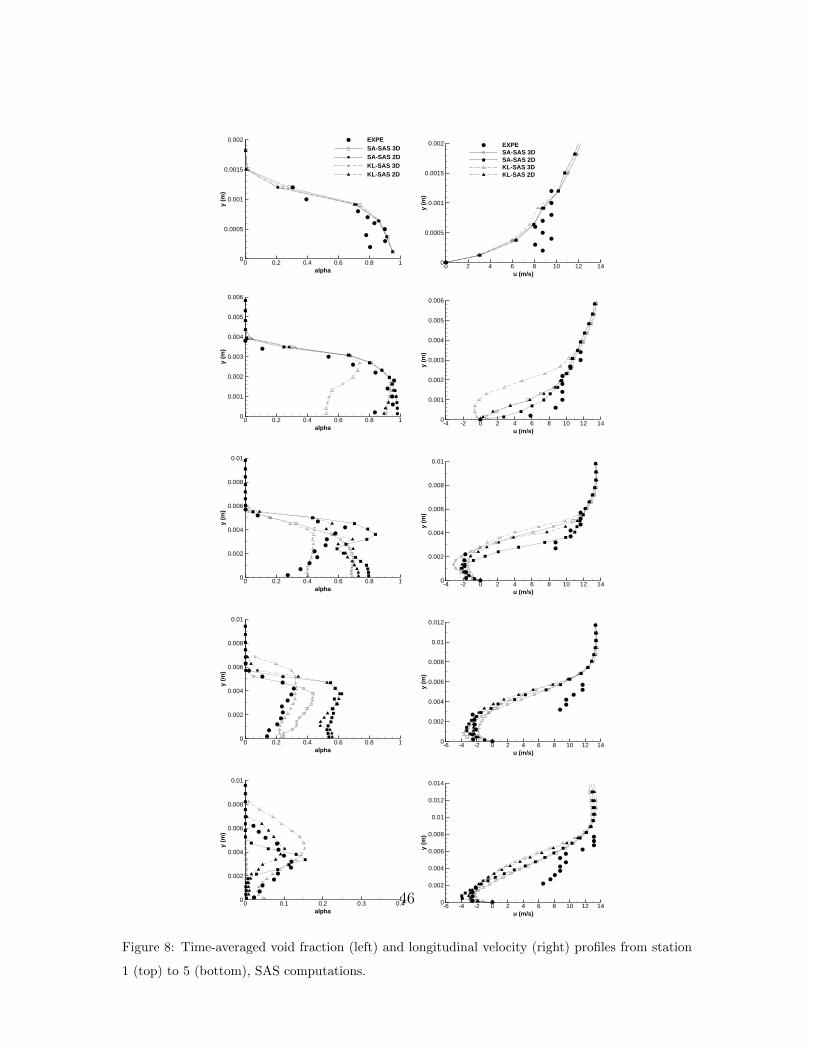
4.2.1. SAS computations
At station 1 (Fig.8), both the time-averaged velocity and void fraction are similar
between 2D and 3D computations. At station 2, the k − ℓ SAS computation under-
estimates the void fraction due to the presence of a re-entrant jet along the bottom
wall, which is not observed experimentally. At station 3 and 4, the void fraction
predicted by the 3D computations is lower than in the 2D computations. About
the velocity u, 3D computations do not have the same behaviour compared with
2D computations. The Spalart-Allmaras SAS 3D computation leads to a stronger
and thicker re-circulation compared with the 2D computation, whereas the k − ℓ
SAS 3D computation minimizes the re-circulation intensity compared with the 2D
computation. Finally, at station 5, the SA SAS 3D computation does not predict
void fraction, which is not the case for the 2D computation. For the k − ℓ SAS
computations, 3D simulation provides a void fraction higher than the 2D solution.
The time-averaged wall pressure, plotted in Figure 9, does not evolved in the same
way for the 3D computations. Indeed, the inlet cavitation number σinlet is higher for
the 3D computations than the 2D computations, therefore, we expect that the mean
wall pressure be higher for the 3D computations than the 2D ones. However, if this
is the case for the computation with the Spalart-Allmaras SAS model, the opposite
occurs with the k − ℓ SAS model.
The RMS wall pressure fluctuations (Fig.9) put in evidence large discrepancies be-
tween 2D and 3D computations. For the 2D computations, the peak of fluctuations
is correctly located with an amplitude in agreement with the experimental measure-
ments. Moreover, the decrease of the fluctuations level in the wake of the cavitation
sheet is well captured. This is not the case for the 3D computations since the level
of pressure fluctuations is largely overestimated in the wake.
22

4.2.2. DES computations
The time-averaged profiles for the void fraction and the longitudinal velocity are
displayed in Figure 10. At the first two stations, the profiles are the same for the 2D
and 3D calculations. At station 3, the 3D computation predicts a void fraction lower
and a re-circulation slightly thicker than the 2D solution. At station 4, contrary to
the 2D computation, the 3D calculation provides a void fraction and a longitudinal
velocity close to the experimental one. Finally, at station 5, as previously observed
with the SA SAS model, the 3D computation under-estimated the cavitation sheet
length since no vapour is present at this station. This is linked to a smoother re-
entrant jet in the 3D computation in comparison with the 2D case.
The time-averaged wall pressure profile and RMS fluctuations, plotted in Figure
11, show large discrepancy between the 2D and the 3D computations. The 3D
computation under-estimates the wall pressure by a factor of three compared with
the experiment and the 2D calculation. Similarly to SAS simulations, the RMS
pressure fluctuations present a large value in the wake of the cavity for the 3D
computation.
4.2.3. Partial conclusions
The time-averaged void fraction and velocity profiles show some small discrepan-
cies between 2D and 3D computations particularly in the re-circulation area. Nev-
ertheless, the re-entrant jet is well captured whatever the dimension of the domain.
Moreover, a part of the difference can be explained by the fact that comparisons are
done for different inlet cavitation numbers.
The wall pressure analysis put in evidence a 3D effect on the dynamic behaviour of
the cavitation sheet. Mainly, the intensity of the pressure fluctuations are overesti-
mated in the sheet as well as in the wake. Further reasons can be invoke to explain
23

these discrepancies between the 2D and 3D compuations. Firstly, the considered cav-
itation model (barotropic model) has never been tested in such 3D cavitating flows.
It has been calibrated with 2D simulations. Maybe the link between the pressure and
the density is too strong to simulate the 3D behaviour. Secondly, we assumed that
the Boussinesq assumption is available with a relation between the mixture Reynolds
tensor and the center of volume averaged velocity gradient. Maybe the assumptions
are too strong in 3D cavitating flows. Additional experimental or numerical data are
needed.
Therefore, 3D effects plays a role in the dynamic of the cavitation sheet even if both
the velocity and void fraction profiles, where measurements are available, are not
strongly affected. Indeed, it seems that 3D effects as we can see on the pressure fluc-
tuations are essentially presented in the wake region located downstream the station
of measurements. These effects manifest also by the low frequency pointed out on
the vapour volume signal.
4.3. Analysis of the oblique mode
From the 3D computations performed with the Spalart-Allmaras SAS model, a
global view of the dynamic of the cavitation sheet is displayed (statistical treatment
on 2.2 seconds). Secondly, a deeper analysis is proposed with distributions and
correlations in the mid-span section and a cross section (statistical treatment on
0.45 second only).
4.3.1. Global analysis
As shown before in Figure 4, the cavitation sheet is not symmetric in the spanwise
direction and grows alternatively from one side of the Venturi to the other. The
intensity of the cross flow is dampened away from the bottom wall, which confirms
the role plays by the cavitation sheet in the formation of this flow. The structure of
24

the flow in the cavitation sheet is studied using a longitudinal cutting plane located
at distance y = 0.001 m from the bottom wall. Six snapshots of the sheet are shown
in Figure 12. The time between two snapshots is approximately T0 = T6≈ 0.028
second where T is the period of the oblique mode. The asymmetry of the cavitation
sheet and the velocity field are well exhibited. At t = 0, the sheet is asymmetric
with an attached cavity (defined by a void fraction higher than 0.9) expands to
x = 0.06 m on the side z = 0.05m and only to x = 0.03 m on the other side. At
the center of the Venturi, the re-entrant jet develops more upstream than at the
walls. The presence of the side walls can explain such a behaviour. Firstly, for the
flow upstream the Venturi throat, the sheet is equivalent to an obstacle. To by-pass
this obstacle, two possibilities are offered to it: to pass over the cavity or to pass
along the side walls. Forcing the pass leads to an acceleration of the flow (Fig.13)
confined between the cavitation sheet and the wall, which plays the role of a small
local venturi. Consequently, the momentum energy of the flow is increased, allowing
it to better resist to the re-entrant jet. Secondly, the side walls involve the formation
of corner vortices (Fig.7), which deflect the re-entrant jet to the center. Therefore,
the re-entrant momentum energy is enforced at the center, which allows it to develop
deeper.
At t = T0
6, the re-entrant jet leads to the cavity decrease along the side z = 0.05m
whereas the cavitation sheet is growing along the opposite wall. At t = 2T0
6, the
re-entrant jet on the side z = 0.05m is deflected to the center of the Venturi. On the
other side, the cavitation sheet follows its growth. At t = 3T0
6, the cavitation sheet
reaches its maximum length on the side z = 0 and a liquid re-entrant jet appears. On
the opposite side, the vortex corner begins to expand, taking with it the sheet. At
t = 4T0
6, the re-entrant jet along the side z = 0 makes face to the vortex corner and
is deflected to the center. Along the other side, the cavitation sheet lengthens. At
25

t = 5T0
6, the re-entrant jet on the side z = 0 flows to the center of the Venturi, while
on the opposite side no re-entrant jet is observed and the cavitation sheet reaches its
maximum length.
Figure 13 shows the time-averaged velocity and void ratio evolutions in the spanwise
direction at different abscissa (x = 0.0083 m and x = 0.02 m inside the attached
cavity and x = 0.027 m at the end of the attached cavity). The void fraction increases
along the side walls due to the fact that the corner vortex sucks a part of stable cavity,
which has to make faced to the re-entrant jet.
4.3.2. Analysis in the mid-span section
The analysis focuses on both the longitudinal and cross components of the ve-
locity. Except for the longitudinal velocity, no comparisons can be done with the
experiments.
In the experimental data, due the non gaussian distribution of the longitudinal veloc-
ity inside the cavitation sheet, the most probable values were chosen for the longitudi-
nal velocity profiles instead of time-averaged values. In order to verify the capability
of computations to capture a part of this non gaussian distribution, we extracted
the distributions of the resolved fluctuating part of both the longitudinal and cross
velocities at all measurement stations. These distributions are plotted in Figures 14
and 15 at stations 3 to 5. Four altitudes are selected: one in the re-circulation area
(y = 0.7 mm), two in the shear stress layer (y = 2 mm and y = 4 mm) and one out
of the cavitation sheet (y = 8.5 mm). The distribution of the velocities is closed to
be gaussian at station 5 and for all the stations at the distance y = 8.5 mm. On the
other hand, in the cavitation sheet, the distribution are not gaussian and displayed
a large interval of probable values. For instance, the distribution of the longitudinal
velocity at station 3 and at the distance y = 4 mm from the bottom wall shows a
26

plateau of probable values from 6 to 11 m/s. For the cross velocity, the large dis-
crepancy between the probable value makes appear often two peaks: one located in
the negative values and the other located in the positive values. This observation is
correlated with the cross instability mentioned above.
The RMS velocity fluctuations and the comparison between mean and most probable
values are illustrated in Figure 16 for the five stations of measurement. At stations
1 and 2, the mean and the most probable longitudinal velocity profiles are closed
one to each other. The RMS values of the resolved part of the velocity field are of
the same order of magnitude in each direction, which means that the turbulence is
isotropic. From stations 3 to 5, the velocity field shows a non gaussian behaviour.
Indeed, the mean and most probable profiles differ particularly in the shear stress
region. For instance, at station 3, the gap between the most probable and the mean
value can reach 2 m/s. For the RMS velocity fluctuations, the fluctuations in the
longitudinal direction are largely higher in comparison with values in the orthogonal
and cross directions. At station 3, the ratio urms/vrms can be close to 10. There-
fore, the turbulence can not be considered as isotropic in the re-circulating area. At
station 5, the gap between the most probable value and the mean value reduces and
the fluctuation comes back to an isotropic behaviour.
To conclude, the analysis in the mid-span section put in evidence that the velocity
field is not gaussian in the re-circulation area and the turbulence at large-scales can
not be considered as isotropic. Out of the re-circulation area, the velocity field is
gaussian and the large-scales turbulence is isotropic.
27

4.3.3. Analysis in a transversal cutting plane
The analysis in a transversal cutting plane located at station 3 (abscissa x = 38
mm) inside the re-circulation zone is proposed. Three instantaneous snapshots of the
void ratio and the velocity vector are depicted in Figure 17. Only an enlargement
near the side z = 0 is presented. For these pictures, the scale of the void ratio is
greater than 1 to improve the contrast of visualizations. A preliminary portrait of
the flow can be derived. Firstly, the corner vortex is 5 mm large and seems to be
weakly affected by the cross flow. These vortices play two roles: in one hand, they
capture a part of the outer flow and feed the sheet in vapour, on the other hand, they
deflect the liquid re-entrant jet to the center of the Venturi. Secondly, the cross flow
is located in the re-circulation area whereas out of the cavitation sheet, the velocity
vectors do not show a global alignment with a strong intensity. Therefore, the shear
stress induced by the re-entrant jet leads to a de-correlation of the flow between the
cavitation sheet and the outer flow.
Spatial two-point correlations based on the void fraction and the longitudinal and
cross velocities have been calculated along the span. Three different distances from
the bottom wall have been considered: y = 5 mm, y = 6.4 mm and y = 7.2 mm.
Along the spanwise, three different points have been chosen in order to verify the
width on which the flow can be considered to be two-dimensional. The considered
reference points are located at the third, the half and the two-third of the span,
respectively. These correlations are presented in Figure 18. For the extreme points,
the longitudinal velocity and void fraction correlations are very low compared with
the cross velocity correlation. Therefore, we conclude that the re-entrant jet is not
coherent in the cavitation sheet and the cross flow is a motion over all the span. At
mid-span, correlations show that the re-entrant jet is correlated over a distance of
28

5 mm on each side of the mid-point. Over this distance, the correlations decrease,
which is not the case for the cross velocity. Once more, the cross velocity shows only
a slight decrease of the correlation over the span (excepted at the distance y = 6.4
mm) that confirms the presence of a global cross motion in the cavitation sheet.
Correlations between the two lateral sides have been also evaluated for the longi-
tudinal velocity and the void ratio. The temporal evolution is presented in Figure
19. It is noticeable that the void fraction and the longitudinal velocity correlations
superimpose. Therefore, the re-entrant jet and the evolution of the cavity are linked
one to each other. The analysis of the correlated signal put in evidence the low
frequency of 6 Hz and a phase difference close to π and confirms that the cavitation
sheet evolves in an opposite phase between the two sides of the Venturi.
5. Conclusion
In the present study, 2D and 3D computations of a cavitation sheet developing
along the bottom wall of a Venturi geometry have been performed using the DES
approach and Scale-Adaptive models. The DES model has undergone a modification
of the constant CDES since the standard value was replaced by 0.9, which allowed to
capture a cavitation sheet behaviour in agreement with the experimental one.
First, comparisons between 2D and 3D (in the mid-span section) computations were
presented together with the experimental results. The mean void fraction and the
mean longitudinal velocity profile exhibited very small discrepancies between the 2D
and the 3D computations. On the contrary, the mean pressure profile and the RMS
pressure fluctuations at the bottom wall put in evidence large differences between 2D
and 3D computations. Overall, 3D computations tend to underestimate the pressure
in the wake of the cavitation sheet, whereas the RMS pressure fluctuations are over-
estimated in the cavitation sheet and in the wake. Indeed, downstream the cavitation
29

sheet, the 3D computations provide a plateau of RMS pressure fluctuations, which
is not observed experimentally or computed by the 2D simulations. The dynamic
behaviour of the cavitation sheet changes between the 2D and 3D computations.
The 3D computations were analyzed in more details. A cross instability at low
frequency (around 6 Hz) was illustrated corresponding to a cross flow inside the re-
circulation area and leading to a growth of the cavitation sheet in an opposite phase
between the two Venturi sides. This results are in agreement with recent observations
provided by an experimental study of a pulsating cavitation sheet over a NACA0015
hydrofoil [9]. From the numerical computations, the main reason to explain this
phenomenon comes from the presence of a vortex at each side of the Venturi, which
modify the structure of the cavitation sheet. These vortices suck a part of the flow
allowing a larger growth of the cavity and deflects the re-entrant jet to the center of
the geometry. It was observed that the thickness of the vortex was almost constant
in time and close to 5 mm. The cross flow takes place in all the re-circulation area
as it is confirmed by the high level of the spanwise velocity correlations through the
cavitation sheet. On the contrary, the re-entrant jet is not uniform in the spanwise
direction but only in a section laying from z = 0.02 m to z = 0.03 m.
On the other hand, the analysis of the longitudinal and spanwise velocity distri-
butions made appear a turbulent flow that is not isotropic and gaussian in the re-
circulation zone. Consequently, the most probable value of the longitudinal velocity
differs from the mean value and the RMS fluctuations of the resolved longitudinal
velocity are larger than the other components.
From this investigation, 3D effects are suggested through the presence of corner vor-
tices and a cross instability. Moreover, a non canonical turbulent flow is shown in
the re-circulation zone, which can be an explanation for the inability of the standard
turbulence models to capture the unsteady behaviour of the cavitation sheet. Even
30

if the pressure fluctuations obtained with the 3D computations are less accurate,
several lessons can be drawn:
• enhanced turbulence models are needed to capture the behaviour of unsteady
cavities (particularly the re-entrant jet),
• side-wall effects have an major influence on the cavity growth and the flow
downstream the cavity,
• the investigation of the sheet dynamics can not restrain itself to the evaluation
of mean quantities and has to focus on resolved fluctuations.
Finally, additional experimental measurements or computations will be welcome to
attest the presented results and to better understand the phenomenon.
Acknowledgement
The authors wish to thank the IDRIS - CNRS supercomputing center for provid-
ing us their computing resources.
31

References
[1] K. Laberteaux, S. Ceccio, Partial cavity flows. Part1. Cavities forming on models
without spanwise variation, Journal of Fluid Mechanics 431 (2001) 1–41.
[2] D. de Lange, G. Bruin, L. van Wijngaarden, On the mechanism of cloud cavi-
tation - experiments and modelling, in: 2nd International Symposium on Cavi-
tation CAV1994, Tokyo, Japan, 1994.
[3] Y. Kawanami, H. Kato, H. Yamaguchi, M. Tanimura, Y. Tagaya, Mechanism
and control of cloud cavitation, Journal of Fluids Engineering 119 (4) (1997)
788–794.
[4] G. Reisman, Y.-C. Wang, C. Brennen, Observations of shock waves in cloud
cavitation, Journal of Fluid Mechanics 355 (1998) 255–283.
[5] S. Gopalan, J. Katz, Flow structure and modeling issues in the closure region
of attached cavitation, Physics of Fluids 12 (4) (2000) 895–911.
[6] D. de Lange, G. de Bruin, Sheet cavitation and cloud cavitation, re-entrant jet
and three-dimensionality, Applied Scientific Research (1998) 91–114.
[7] K. Laberteaux, S. Ceccio, Partial cavity flows. Part2. Cavities forming on test
objects with spanwise variation, Journal of Fluid Mechanics 431 (2001) 43–63.
[8] E. Foeth, C. van Doorne, T. van Terwisga, B. Wienecke, Time-resolved PIV
and flow visualization of 3D sheet cavitation, Experiments in Fluids 40 (2006)
503–513.
32

[9] S. Prothin, J.-Y. Billard, H. Djeridi, Image processing using POD and DMD
for the study of cavitation development on a NACA0015, in: 13th Journees de
l’Hydrodynamique, Laboratoire Saint-Venant, Chatou, France, 2012.
[10] G. Schnerr, I. Sezal, S. Schmidt, Numerical investigation of three-dimensional
cloud cavitation with special emphasis on collapse induced shock dynamics,
Physics of Fluids 20 (2008) 040703.
[11] A. Koop, H. Hoeijmakers, Unsteady sheet cavitation on three-dimensional hy-
drofoil, in: 7th International Conference on Multiphase Flow, Tampa, USA,
2010.
[12] S. Park, S. Hyung Rhee, Numerical analysis of the three-dimensional cloud
cavitating flow around a twisted hydrofoil, Fluid Dynamics Research 45 (1)
(2013) 1–20.
[13] G. Wang, M. Ostoja-Starzewski, Large eddy simulation of a sheet/cloud cav-
itation on a NACA0015 hydrofoil, Applied Mathematical Modeling 31 (2007)
417–447.
[14] N. Dittakavi, A. Chunekar, S. Frankel, Large eddy simulation of turbulent-
cavitation interactions in a Venturi nozzle, Journal of Fluids Engineering
132 (12) (2010) 121301.
[15] R. Bensow, G. Bark, Simulating cavitating flows with LES in openfoam, in: V
ECCOMAS CFD, Lisbon, Portugal, June 2010.
[16] N.-X. Lu, R. Bensow, G. Bark, LES of unsteady cavitation on the Delft twisted
foil, Journal of Hydrodynamics, serie B 22 (5) (2010) 784–790.
33

[17] P. Spalart, Detached-eddy simulation, Annual Review of Fluid Mechanics 41
(2009) 181–202.
[18] R. Kunz, J. Lindau, T. Kaday, L. Peltier, Unsteady RANS and detached-eddy
simulations of cavitating flow over a hydrofoil, in: 5rd International Symposium
on Cavitation CAV2003, Osaka, Japan, 2003.
[19] M. Kinzel, J. Lindau, L. Peltier, R. Kunz, S. Venkateswaran, Detached-eddy
simulations for cavitating flows, in: AIAA-2007-4098, 18th AIAA Computa-
tional Fluid dynamics Conference, Miami, USA, 2007.
[20] R. Bensow, Simulation of the unsteady cavitation on the Delft twist11 foil using
RANS, DES and LES, in: Second International Symposium on Marine Propul-
sors, Hamburg, Germany, June 2011.
[21] B. Ji, X. Luo, X. Peng, H. Xu, Partially-averaged Navier-Stokes method with
modified k − ε model for cavitating flow around a marine propeller in a non-
uniform wake, Int. Journal of Heat and Mass Transfer 55 (2012) 6582–6588.
[22] B. Ji, X. Luo, Y. Wu, X. Peng, Y. Duan, Numerical analysis of unsteady cavi-
tating turbulent flow and shedding horse-shoe vortex structure around a twisted
hydrofoil, International Journal of Multiphase Flow 51 (2013) 33–43.
[23] E. Goncalves, R. F. Patella, Numerical simulation of cavitating flows with ho-
mogeneous models, Computers & Fluids 38 (9) (2009) 1682–1696.
[24] E. Goncalves, Numerical study of unsteady turbulent cavitating flows, European
Journal of Mechanics B/Fluids 30 (1) (2011) 26–40.
34

[25] J. Decaix, E. Goncalves, Time-dependent simulation of cavitating flow with
k−ℓ turbulence models, Int. Journal for Numerical Methods in Fluids 68 (2012)
1053–1072.
[26] F. Menter, The scale-adaptive simulation method for unsteady turbulent flow
predictions. Part 1: Theory and model description, Flow, Turbulence and Com-
bustion 85 (1) (2010) 113–138.
[27] C. Ishii, T. Hibiki, Thermo-fluid dynamics of two-phase flow, Springer (2006).
[28] Y. Delannoy, J. Kueny, Two phase flow approach in unsteady cavitation mod-
elling, in: Cavitation and Multiphase Flow Forum, ASME-FED, vol. 98, pp.153-
158, 1990.
[29] H. Guillard, C. Viozat, On the behaviour of upwind schemes in the low Mach
number limit, Computers & Fluids 28 (1) (1999) 63–86.
[30] E. Turkel, Preconditioned methods for solving the incompressible and low speed
compressible equations, Journal of Computational Physics 172 (2) (1987) 277–
298.
[31] J.-L. Reboud, B. Stutz, O. Coutier, Two-phase flow structure of cavitation:
experiment and modelling of unsteady effects, in: 3rd International Symposium
on Cavitation CAV1998, Grenoble, France, 1998.
[32] O. Coutier-Delgosha, J. Reboud, Y. Delannoy, Numerical simulation of the un-
steady behaviour of cavitating flow, Int. Journal for Numerical Methods in Flu-
ids 42 (2003) 527–548.
[33] Y. Chen, C. Lu, L. Wu, Modelling and computation of unsteady turbulent
cavitation flows, Journal of Hydrodynamics 18 (5) (2006) 559–566.
35

[34] L. Zhou, Z. Wang, Numerical simulation of cavitation around a hydrofoil and
evaluation of a RNG k − ε model, Journal of Fluid Engineering 130 (1) (2008)
011302.
[35] P. Spalart, W. Jou, M. Strelets, S. Allmaras, Comments on the feasibility of
LES for wings and on hybrid RANS//LES approach, in: 1st AFSOR Int. Conf.
on DNS/LES - Ruston, 1997.
[36] P. Spalart, S. Deck, M. Shur, K. Squires, M. Strelets, A. Travin, A new version
of detached-eddy simulation, resistant to ambiguous grid densities, Theoretical
Computational Dynamics 20 (2006) 181–195.
[37] F. Menter, Y. Egorov, A scale-adaptive simulation model using two-equation
models, in: AIAA 2005–1095, 43rd Aerospace Science Meeting and Exhibit,
Reno, Nevada, 2006.
[38] J. Rotta, Turbulente Strmumgen, BG Teubner Stuttgart, 1972.
[39] F. Menter, The scale-adaptive simulation method for unsteady turbulent flow
predictions. Part 2: Application to complex flows, Flow, Turbulence and Com-
bustion 85 (1) (2010) 139–165.
[40] L. Davidson, Evaluation of the SST-SAS model: channel flow, asymmetric dif-
fuser and axi-symmetric hill, in: Proceedings of ECCOMAS CFD 2006, Egmond
aan Zee, The Netherlands, 2006.
[41] B. Smith, The k − kl turbulence model and wall layer model for compressible
flows, in: AIAA 90–1483, 21st Fluid and Plasma Dynamics Conference – Seattle,
Washington, 1990.
36

[42] F. Menter, Eddy viscosity transport equations and their relation to the k − ǫ
model, Journal of Fluids Engineering 119 (1997) 876–884.
[43] E. Goncalves, J. Decaix, Wall model and mesh influence study for partial cavi-
ties, European Journal of Mechanics B/Fluids 31 (1) (2012) 12–29.
[44] J. Viegas, M. Rubesin, Wall–function boundary conditions in the solution of
the Navier–Stokes equations for complex compressible flows, in: AIAA 83–1694,
16th Fluid and Plasma Dynamics Conference – Danver, Massachussetts, 1983.
[45] A. Jameson, W. Schmidt, E. Turkel, Numerical solution of the Euler equations
by finite volume methods using Runge-Kutta time stepping schemes, in: AIAA
Paper 81–1259, 1981.
[46] P. Roe, Approximate Riemann solvers, parameters vectors, and difference
schemes, Journal of Computational Physics 43 (1981) 357–372.
[47] S. Tatsumi, L. Martinelli, A. Jameson, Flux-limited schemes for the compressible
Navier-Stokes equations, AIAA Journal 33 (2) (1995) 252–261.
[48] S. Barre, J. Rolland, G. Boitel, E. Goncalves, R. F. Patella, Experiments and
modelling of cavitating flows in Venturi: attached sheet cavitation, European
Journal of Mechanics B/Fluids 28 (2009) 444–464.
37

Table 1: Numerical computations.
Turbulence model Dimension of the domain σinlet Frequency (Hz)
k − ℓ SAS 2D 0.580 no particular frequency
k − ℓ SAS 3D 0.590 ≈ 6
SA-SAS 2D 0.588 no particular frequency
SA-SAS 3D 0.6 ≈ 6
SA-DES 2D 0.588 no particular frequency
SA-DES 3D 0.6 ≈ 3
38

Figure 1: Schematic view of the 4◦ Venturi profile.
39

x (m)
y(m
)
-0.05 0 0.05 0.1 0.15
-0.02
0
0.02
0.04
0.06
X
Y
Z
inlet
outlet
Figure 2: View of the 2D mesh near the Venturi throat and view of the 3D mesh.
40

x (m)
y (m
)
0 0.02 0.04 0.06 0.08 0.1
0
0.02
0.04
0.06
x (m)
y (m
)
0 0.02 0.04 0.06 0.08 0.1
0
0.02
0.04
0.06
Figure 3: View of the RANS (black) ans LES (white) regions in the mid-span section for the DES
computations with CDES = 0.65 (top) and CDES = 0.9 (bottom).
41

x (m)
z(m
)
0 0.01 0.02 0.03 0.04 0.05-0.01
0
0.01
0.02
0.03
0.04
0.05
0.06Grad-rho: 30000 60000 90000 120000 150000 180000 210000 240000 270000 300000
x (m)
z(m
)
0 0.01 0.02 0.03 0.04 0.05-0.01
0
0.01
0.02
0.03
0.04
0.05
0.06Grad-rho: 30000 60000 90000 120000 150000 180000 210000 240000 270000 300000
x (m)
z(m
)
0 0.01 0.02 0.03 0.04 0.05 0.06 0.07 0.08-0.01
0
0.01
0.02
0.03
0.04
0.05
0.06Grad-rho: 30000 60000 90000 120000 150000 180000 210000 240000 270000 300000
x (m)
z(m
)
0 0.01 0.02 0.03 0.04 0.05-0.01
0
0.01
0.02
0.03
0.04
0.05
0.06Grad-rho: 30000 60000 90000 120000 150000 180000 210000 240000 270000 300000
x (m)
z(m
)
0 0.01 0.02 0.03 0.04 0.05-0.01
0
0.01
0.02
0.03
0.04
0.05
0.06Grad-rho: 30000 60000 90000 120000 150000 180000 210000 240000 270000 300000
x (m)
z(m
)
0 0.01 0.02 0.03 0.04 0.05 0.06 0.07 0.08-0.01
0
0.01
0.02
0.03
0.04
0.05
0.06Grad-rho: 30000 60000 90000 120000 150000 180000 210000 240000 270000 300000
Figure 4: Gradient density modulus visualization at two different instants: k−ℓ SAS (top), Spalart-
Allmaras SAS (middle) and DES (bottom), 3D computations.
42

X
Y
Z
X
Y
Z
X
Y
Z
X
Y
Z
X
Y
Z
X
Y
Z
Figure 5: Iso-surface of the void fraction for the value of 60% at two different instants: k − ℓ SAS
(top), Spalart-Allmaras SAS (middle) and DES (bottom), 3D computations.
43

x0 0.5 1
w: -1 -0.8 -0.6 -0.4 -0.2 0 0.2 0.4 0.6 0.8 1
0 0.5 1
x
X
YZ
w: -0.5 -0.4 -0.3 -0.2 -0.1 0 0.1 0.2 0.3 0.4 0.5
Figure 6: Transversal component w of velocity field, SA-SAS (top) and SA-DES (bottom) located
at 10−3 m from the bottom wall.
44

z
y
0 0.005 0.01 0.015 0.02 0.025 0.03 0.035 0.04 0.045 0.050.004
0.006
0.008
0.01
0.012
0.014
z
y
0 0.005 0.01 0.015 0.02 0.025 0.03 0.035 0.04 0.045 0.050.004
0.006
0.008
0.01
0.012
0.014
k − ℓ SAS simulation
SA DES simulation
Figure 7: Void fraction and velocity vector at two different instants in a transversal cutting plane
at station 3, k − ℓ SAS (left) and SA-DES (right).
45
alpha
y (m
)
0 0.2 0.4 0.6 0.8 10
0.0005
0.001
0.0015
0.002 EXPESA-SAS 3DSA-SAS 2DKL-SAS 3DKL-SAS 2D
alpha
y (m
)
0 0.2 0.4 0.6 0.8 10
0.001
0.002
0.003
0.004
0.005
0.006
alpha
y (m
)
0 0.2 0.4 0.6 0.8 10
0.002
0.004
0.006
0.008
0.01
alpha
y (m
)
0 0.2 0.4 0.6 0.8 10
0.002
0.004
0.006
0.008
0.01
alpha
y (m
)
0 0.1 0.2 0.3 0.40
0.002
0.004
0.006
0.008
0.01
u (m/s)
y (m
)
0 2 4 6 8 10 12 140
0.0005
0.001
0.0015
0.002 EXPESA-SAS 3DSA-SAS 2DKL-SAS 3DKL-SAS 2D
u (m/s)y
(m)
-4 -2 0 2 4 6 8 10 12 140
0.001
0.002
0.003
0.004
0.005
0.006
u (m/s)
y (m
)
-4 -2 0 2 4 6 8 10 12 140
0.002
0.004
0.006
0.008
0.01
u (m/s)
y (m
)
-6 -4 -2 0 2 4 6 8 10 12 140
0.002
0.004
0.006
0.008
0.01
0.012
u (m/s)
y (m
)
-6 -4 -2 0 2 4 6 8 10 12 140
0.002
0.004
0.006
0.008
0.01
0.012
0.014
Figure 8: Time-averaged void fraction (left) and longitudinal velocity (right) profiles from station
1 (top) to 5 (bottom), SAS computations.
46

x-x i (m)
(P-P
v)/P
v
0.1 0.15 0.2 0.25 0.3-2
0
2
4
6
8
10
12
14
16 EXPSA-SAS 3DSA-SAS 2DKL-SAS 3DKL-SAS 2D
x-x inlet (m)
P’ r
ms
/ Pm
ean
0.15 0.2 0.25 0.30
0.1
0.2
0.3
0.4
0.5
0.6
0.7
0.8 EXPSA-SAS 3DSA-SAS 2DKL-SAS 3DKL-SAS 2D
Figure 9: Time-averaged wall pressure (top) and RMS fluctuations (bottom) along the bottom wall,
SAS computations.
47

alpha
y (m
)
0 0.2 0.4 0.6 0.8 10
0.001
0.002
0.003 EXPEDES 3DDES 2D
alpha
y (m
)
0 0.2 0.4 0.6 0.8 10
0.001
0.002
0.003
0.004
0.005
0.006
0.007
0.008
alpha
y (m
)
0 0.2 0.4 0.6 0.8 10
0.001
0.002
0.003
0.004
0.005
0.006
0.007
0.008
alpha
y (m
)
0 0.2 0.4 0.60
0.001
0.002
0.003
0.004
0.005
0.006
0.007
0.008
0.009
0.01
alpha
y (m
)
0 0.1 0.2 0.3 0.40
0.002
0.004
0.006
0.008
0.01
u (m/s)
y (m
)
0 2 4 6 8 10 12 140
0.0005
0.001
0.0015
0.002
0.0025
0.003
0.0035
0.004EXPEDES 3DDES 2D
u (m/s)y
(m)
0 2 4 6 8 10 12 140
0.0005
0.001
0.0015
0.002
0.0025
0.003
0.0035
0.004
u (m/s)
y (m
)
-4 -2 0 2 4 6 8 10 12 140
0.001
0.002
0.003
0.004
0.005
0.006
0.007
0.008
u (m/s)
y (m
)
-6 -4 -2 0 2 4 6 8 10 12 140
0.002
0.004
0.006
0.008
0.01
u (m/s)
y (m
)
-4 -2 0 2 4 6 8 10 12 140
0.002
0.004
0.006
0.008
0.01
0.012
0.014
Figure 10: Time-averaged void fraction (left) and longitudinal velocity (right) profiles from station
1 (top) to 5 (bottom), DES computations.
48

x-x i (m)
(P-P
v)/P
v
0.1 0.15 0.2 0.25 0.3-2
0
2
4
6
8
10
12
14
16 EXPDES 3DDES 2D
x-x i (m)
P’ r
ms
/ Pav
0.15 0.2 0.25 0.30
0.1
0.2
0.3
0.4
0.5
0.6
0.7 EXPDES 3DDES 2D
Figure 11: Time-averaged wall pressure (top) and RMS fluctuations (bottom) along the bottom
wall, DES computations.
49

x
z
0 0.02 0.04 0.06 0.08
0.01
0.02
0.03
0.04
0.05
0.06
alpha: 0.06 0.12 0.18 0.25 0.31 0.37 0.43 0.49 0.55 0.61 0.67 0.74 0.80 0.86 0.92
t = 0
x
z
0 0.02 0.04 0.06 0.08
0.01
0.02
0.03
0.04
0.05
0.06
t = 2T0
x
z
0 0.02 0.04 0.06 0.08
0.01
0.02
0.03
0.04
0.05
0.06
t = 4T0
x
z
0 0.02 0.04 0.06 0.08
0.01
0.02
0.03
0.04
0.05
0.06
t = T0
x
z
0 0.02 0.04 0.06 0.08
0.01
0.02
0.03
0.04
0.05
0.06
t = 3T0
x
z
0 0.02 0.04 0.06 0.08
0.01
0.02
0.03
0.04
0.05
0.06
t = 5T0
Figure 12: Void fraction and velocity vector at six different instants, in a cutting plane located at
y = 10−3 m.
50

z (m)
u(m
/s)
0 0.01 0.02 0.03 0.04 0.055
5.5
6
6.5
7
7.5
8
8.5
9
9.5
10
z (m)
u(m
/s)
0 0.01 0.02 0.03 0.04 0.050
1
2
3
4
5
6
7
8
z (m)
u(m
/s)
0 0.01 0.02 0.03 0.04 0.050
1
2
3
4
5
6
7
velocity component u
z (m)
Alp
ha
0 0.01 0.02 0.03 0.04 0.050
0.1
0.2
0.3
0.4
0.5
0.6
0.7
0.8
0.9
1
z (m)
Alp
ha
0 0.01 0.02 0.03 0.04 0.050.5
0.6
0.7
0.8
0.9
1
z (m)
Alp
ha
0 0.01 0.02 0.03 0.04 0.050.5
0.6
0.7
0.8
0.9
1
void ratio α
Figure 13: Time-averaged longitudinal velocity (left) and void fraction (right) profiles in the span
direction at distance y = 10−3 m and abscissa x = 8.3 10−3 m (top) ; x = 210−2 m (middle) and
x = 2.7 10−2 m (bottom).
51

station 3 station 4 station 5
Figure 14: Distribution of the longitudinal velocity u from station 3 to 5 (left to right) at four
distances from the bottom wall: y = 0.7 mm ; y = 2 mm ; y = 4 mm and y = 8.5 mm (top to
bottom). (•) refers to the mean value.
52

station 3 station 4 station 5
Figure 15: Distribution of the transversal velocity w from station 3 to 5 (left to right) at four
distances from the bottom wall: y = 0.7 mm ; y = 2 mm ; y = 4 mm and y = 8.5 mm (top to
bottom). (•) refers to the mean value.
53

u (m/s)
y (m
)
0 2 4 6 8 10 12 140
0.001
0.002
0.003
0.004
0.005
0.006
0.007 U-probU-mean
u (m/s)
y (m
)
0 2 4 6 8 10 12 140
0.001
0.002
0.003
0.004
0.005
0.006
0.007 U-probU-mean
u (m/s)
y (m
)
0 5 100
0.001
0.002
0.003
0.004
0.005
0.006
0.007 U-probU-mean
u (m/s)
y (m
)
0 5 100
0.001
0.002
0.003
0.004
0.005
0.006
0.007 U-probU-mean
u (m/s)
y (m
)
0 5 100
0.001
0.002
0.003
0.004
0.005
0.006
0.007 U-probU-mean
u (m/s)
y(m
)
0 0.05 0.1 0.15 0.2 0.25 0.3 0.35 0.40
0.001
0.002
0.003
0.004
0.005
0.006
0.007Urms
Vrms
Wrms
u (m/s)
y(m
)
0 0.1 0.2 0.3 0.4 0.5 0.60
0.001
0.002
0.003
0.004
0.005
0.006
0.007Urms
Vrms
Wrms
u (m/s)
y(m
)
0 0.5 1 1.5 20
0.001
0.002
0.003
0.004
0.005
0.006
0.007Urms
Vrms
Wrms
u (m/s)
y(m
)
0 0.25 0.5 0.75 10
0.001
0.002
0.003
0.004
0.005
0.006
0.007
0.008
0.009Urms
Vrms
Wrms
u (m/s)
y(m
)
0 0.25 0.5 0.75 10
0.001
0.002
0.003
0.004
0.005
0.006
0.007
0.008
0.009Urms
Vrms
Wrms
Figure 16: Time-averaged and most probable longitudinal velocity u (left) and RMS of the resolved
part of the fluctuating velocities (right) in the mid-span from station 1 (top) to 5 (bottom).54

z (m)
y(m
)
0 0.0025 0.005 0.0075 0.01 0.0125 0.015 0.0175 0.020.004
0.006
0.008
0.01
0.012
0.014 alpha: 0.06 0.22 0.38 0.54 0.70 0.86 1.02 1.18 1.34 1.50
z (m)
y(m
)
0 0.0025 0.005 0.0075 0.01 0.0125 0.015 0.0175 0.020.004
0.006
0.008
0.01
0.012
0.014 alpha: 0.06 0.22 0.38 0.54 0.70 0.86 1.02 1.18 1.34 1.50
z (m)
y(m
)
0 0.0025 0.005 0.0075 0.01 0.0125 0.015 0.0175 0.020.004
0.006
0.008
0.01
0.012
0.014 alpha: 0.06 0.22 0.38 0.54 0.70 0.86 1.02 1.18 1.34 1.50
Figure 17: Snapshot of the void ratio and the velocity vector in a transversal cutting plane at
station 3.
55

third-span mid-span two-third-span
Figure 18: Spatial correlations based on the void fraction, the longitudinal and transversal velocities
with three reference points: third-span (left), mid-span (middle) and two-third-span (right) and at
three distances from the bottom wall: y = 5 mm, y = 6.4 mm and y = 7.2 mm (top to bottom).
56

t (s)
Cor
rela
tion
-0.25 -0.2 -0.15 -0.1 -0.05 0 0.05 0.1 0.15 0.2 0.25-1
-0.8
-0.6
-0.4
-0.2
0
0.2
0.4
0.6
0.8
1 alphau
Figure 19: Spatial correlations based on the void fraction and the longitudinal velocity between
two points located on each side of the Venturi.
57