investigation of tension in anchor lines and influence on
TRANSCRIPT

Investigation of tension in anchor lines and influence on vessel behaviour Time domain simulation of Barge response
Petter Svardal Langeland
Master of Science in Ship Design
Submission date: June 2016
Supervisor: Karl Henning Halse
Norwegian University of Science and Technology Ålesund
Faculty of Maritime Technology and Operation


Mandatory statement Each student is responsible for complying with rules and regulations that relate to
examinations and to academic work in general. The purpose of the mandatory statement is to
make students aware of their responsibility and the consequences of cheating. Failure to
complete the statement does not excuse students from their responsibility.
Please complete the mandatory statement by placing a mark in each box for statements 1-6
below.
1. I/we hereby declare that my/our paper/assignment is my/our own
work, and that I/we have not used other sources or received
other help than is mentioned in the paper/assignment.
2. I/we herby declare that this paper
1. Has not been used in any other exam at another department/university/university college
2. Is not referring to the work of others without acknowledgement
3. Is not referring to my/our previous work without acknowledgement
4. Has acknowledged all sources of literature in the text and in the list of references
5. Is not a copy, duplicate or transcript of other work
Mark each
box:
1.
2.
3.
4.
5.
3.
I am/we are aware that any breach of the above will be considered as cheating, and may result in annulment of the examination and exclusion from all universities and university colleges in Norway for up to one year, according to the Act relating to Norwegian Universities and University Colleges, section 4-7 and 4-8 and Examination regulations .
4. I am/we are aware that all papers/assignments may be checked
for plagiarism by a software assisted plagiarism check
5. I am/we are aware that NTNU will handle all cases of suspected
cheating according to prevailing guidelines.
6. I/we are aware of the NTNU’s rules and regulation for using
sources.
Publication agreement
ECTS credits: 30
Supervisor: Karl Henning Halse
Agreement on electronic publication of master thesis Author(s) have copyright to the thesis, including the exclusive right to publish the document (The
Copyright Act §2).
All theses fulfilling the requirements will be registered and published in Brage, with the approval of the
author(s).
Theses with a confidentiality agreement will not be published.
I/we hereby give NTNU the right to, free of
charge, make the thesis available for electronic publication: yes no
Is there an agreement of confidentiality? yes no (A supplementary confidentiality agreement must be filled in and included in this document)
- If yes: Can the thesis be online published when the
period of confidentiality is expired? yes no
This master’s thesis has been completed and approved as part of a master’s degree programme
at NTNU Ålesund. The thesis is the student’s own independent work according to section 6 of
Regulations concerning requirements for master's degrees of December 1st, 2005.
Date: 03.06.16


vii
Abstract
The topic of this thesis is time domain analysis of mooring line effects on a vessels response,
where a barge is used as test model. This type of simulation can be used to investigate and
evaluate how the forces from the mooring line affects the vessels response over time. As an
introduction, some background theory regarding anchor handling and vessel stability is
presented. The objective of the thesis is to show how the mooring line is affecting the vessel
response, mainly heave, pitch and roll.
Both the barge and mooring line is modelled and simulated by using Aquasim, a software
package delivered by Aquastructures. The package includes the programs AquaEdit, AquaBase,
AquaView and AquaTool which are all used as aid in this project. This software is specialized
on mooring analysis related to the aquaculture industry and some offshore operations. For
purely analysing vessel response it is unproven and verifying its suitability is a part of the
project.
The barge model is matched against ShipX, which is a proven software when it comes to vessel
response simulation, to verify that the model is acting realistically. Due to limitations to the
program the model used for this project has some limitations which are reflected upon at the
end of the report.
Different case studies are simulated. The results indicate that there is a connection between the
variations in mooring line force and the vessel response. Worsened environment, mainly
increased wave height and current causes more variations and unpredictability.

viii

ix
Preface
This master thesis is written at the Faculty of Maritime Technology and Operations at NTNU
Ålesund. It represents the end of my days as a student NTNU Ålesund, former AAUC. The
years I have spent in Ålesund and abroad have been rewarding, both academically and socially
as I have learned a lot and made good friends from all over the world.
I would like to thank my supervisor Karl Henning Halse for providing me with this project and
for his good support and advices throughout my work on my thesis. He showed great flexibility
as he always provided other options when things did not go as planned.
______________________________________________________
Petter Svardal Langeland
Ålesund, June 2016

x

xi
Table of contents List of figures ...................................................................................................................... xiii List of tables ........................................................................................................................ xiv
Abbreviations ....................................................................................................................... xv
1 INTRODUCTION ............................................................................................................ 1
1.1 Background .................................................................................................................... 1 1.2 Anchor Handling ............................................................................................................ 2
Anchor Handling Tug Supply vessel (AHTS/AHV) .............................................. 2 Equipment .............................................................................................................. 3 Anchor handling operation ..................................................................................... 3
2 BACKGROUND THEORY ............................................................................................ 5
2.1 Definition of motions ..................................................................................................... 5 2.2 Stability .......................................................................................................................... 6
Righting moment .................................................................................................... 7 GZ-curve ................................................................................................................ 8
Metacentre .............................................................................................................. 8 Longitudinal stability ............................................................................................. 9
2.3 Vessel response ............................................................................................................ 10 Response in regular waves ................................................................................... 10
Strip Theory .......................................................................................................... 11
2.4 Stability criteria ............................................................................................................ 11 General stability criteria ....................................................................................... 12 Special criteria for AHTS ..................................................................................... 12
Mooring forces ..................................................................................................... 13
3 MODELLING APPROACH ......................................................................................... 17
3.1 Software ....................................................................................................................... 17 AquaSim ............................................................................................................... 17
ShipX Vessel Reponses Program ......................................................................... 17 3.2 Barge model ................................................................................................................. 18
Geometry and hydrostatics ................................................................................... 18
Natural roll period ................................................................................................ 19 3.3 Modelling in AquaSim ................................................................................................. 20
Load calculation ................................................................................................... 20 Procedure .............................................................................................................. 21 Properties for the time domain simulations .......................................................... 23
Barge constraints .................................................................................................. 24 Mooring line model .............................................................................................. 25
3.4 Modelling in ShipX ...................................................................................................... 25
4 CASE STUDIES ............................................................................................................. 27
4.1 Case study descriptions ................................................................................................ 27 4.2 Waves and current ........................................................................................................ 27
5 SIMULATION AND RESULTS ................................................................................... 29
5.1 Verification of movements ........................................................................................... 29 5.2 Study Case 1 – AHV close to OI.................................................................................. 31 5.3 Study Case 2 – At drop point ....................................................................................... 34

xii
5.4 Study Case 3 – Anchor in water ................................................................................... 40 5.5 Case study 4 – Angled line with offset from centre ..................................................... 43
6 DISCUSSION ................................................................................................................. 47
6.1 Software ....................................................................................................................... 47 6.2 Barge simplifications .................................................................................................... 47 6.3 Constraints .................................................................................................................... 47
6.4 Differences in roll motion ............................................................................................ 48 6.5 Results .......................................................................................................................... 49
7 CONCLUSION AND FUTURE WORK...................................................................... 51
7.1 Conclusion .................................................................................................................... 51
7.2 Future work .................................................................................................................. 52
REFERENCES ....................................................................................................................... 53
APPENDIX A – MODEL INPUT ........................................................................................... 2
APPENDIX B – CD .................................................................................................................. 7
APPENDIX C – ARTICLE DRAFT ...................................................................................... 9
xiii
List of figures
Figure 1.1 Bourbon Dolphin [www.maritimt.com] ............................................................... 1
Figure 1.2 Island Vanguard from Island Offshore. UT 787 DC design from Rolls-Royce. .. 2
Figure 1.3 Typical deck equipment found on board a AHTS vessel [4] ................................ 3
Figure 2.1 Vessel DOF when encountering wave[8] ............................................................ 5
Figure 2.2 Stable, neutral and unstable condition[5] ............................................................. 6
Figure 2.3 Illustration of a heeling vessel .............................................................................. 7
Figure 2.4 GZ-curve for barge with GM=1.9m and weight 7380 ton. ................................... 8
Figure 2.5 A vessel in a trimming condition, trimming forward ......................................... 10
Figure 2.6 Strip theory.[6] .................................................................................................... 11
Figure 2.7 Back view of vessel ............................................................................................ 13
Figure 2.8 Side and top view of vessel ................................................................................. 13
Figure 2.9 Side view of force components from the mooring setup .................................... 14
Figure 2.10 Aft end of a vessel with the force components ................................................. 15
Figure 3.1 Components of a modelled Barge in AquaSim .................................................. 18
Figure 3.2 Components of a modelled Barge in AquaSim .................................................. 21
Figure 3.3 Cross section for Main element .......................................................................... 22
Figure 3.4 Cross section for 2D hydrodynamic element ...................................................... 22
Figure 3.5 Weather loads as presented in AquaBase ........................................................... 23
Figure 3.6 DOF in nodes on Barge model. 1=free 0=locked ............................................... 25
Figure 3.7 Drawing of hull geometry as presented in ShipX ............................................... 26
Figure 4.1 Simple study cases of AH operation involving OI and AHV ............................. 28
Figure 4.2 Loading conditions for study case 4. Mooring line set at 60 and 36 ................. 28
Figure 5.1 Heave, roll and pitch comparison ....................................................................... 30
Figure 5.2 Case #0 and #1 Comparison of pitch and roll motion at T=6.5s and T=7s. ....... 32
Figure 5.3 Case #1. Pitch motion for T=6.5s and 7s seconds in beam sea. ......................... 33
Figure 5.4 Case #1. Axial force in mooring line acting on the stern in beam sea. ............... 33
Figure 5.5 Pitch and heave motion in head sea .................................................................... 36
Figure 5.6 Case #2. Roll-, pitch-motion and mooring line force at T=6.5s and 7s ............. 37
Figure 5.7 Roll motion with amplitude 1 and 2. Case #2 ..................................................... 38
Figure 5.8 Roll motion and mooring line force with varying amplitudes and with current. 39
Figure 5.9 Case #3. Pitch and Heave motions in head sea ................................................... 41
Figure 5.10 Case #3. Roll-, pitch-motion and mooring line force in beam sea ................... 42
Figure 5.11 Case #4. Roll- and pitch-motion with varying angle on mooring line ............ 44
Figure 5.12 Comparison of roll motion for all study cases based on wave period. ............. 45

xiv
List of tables
Table 2.1 Ship motions and DOF ........................................................................................... 5
Table 3.1 Barge geometry and hydrostatics ......................................................................... 19
Table 3.2 Weather loads and description ............................................................................. 23
Table 3.3 Time series setup in AquaBase ............................................................................ 24
Table 3.4 parameters for anchor line .................................................................................... 25
Table 3.5 parameters for work wire ..................................................................................... 25
Table 5.1 Wave headings and acting motions ...................................................................... 29

xv
Abbreviations
AHV/AHTS Anchor Handling Vessel Tug Supply
BP Bollard pull
CL Centre line of vessel
DNV GL Det norske Veritas Germanische Lloyd
DOF Degree Of Freedom
FEA Finite Element Analysis
G Centre of Gravity
IMO International maritime Organization
OI Offshore Installation
IS code Code on intact stability
K Keel
M Metacentre
NMD Norwegian Maritime Directorate
RAO Response Amplitude Operator
WL Water line

xvi
Nomenclature
Symbol Unit Explanation
𝛼 [deg] Angle between mooring line force and aft end xz-plane
𝛼𝑋𝑍 [deg] Angle between mooring line force and aft end in xz-plane
𝛽 [deg] Angle between mooring line force and centre line xy-plane
𝛽𝑋𝑌 [deg] Angle between mooring line force and centre line xy-plane
Δ [tonnes] Displacement weight
∇ [𝑚3] Displacement volume
𝜁 [𝑚] Wave elevation
𝜁𝑎 - Wave amplitude
𝜂𝑘 - Vessel motion amplitude for given degree of freedom k
𝜂𝑘𝑎 [𝑚] Motion amplitude per unit wave amplitude for a given
degree of freedom k
𝜌 [𝑘𝑔
𝑚3] Water density
𝜃 [deg] Heeling angle
𝜃𝑘 [deg] Phase angle for a given degree of freedom
𝜔 [𝑟𝑎𝑑𝑠⁄ ] Frequency of encounter
𝑎2 [𝑚 𝑠2⁄ ] Fluid acceleration in local y-direction
𝐴𝑟 [𝑚] Amplitude of the reflected wave
B - Centre of Buoyancy
B’ - Centre of Buoyancy after heel
b [𝑚] Breadth
𝐶𝑎𝑦 - Added mass in local y-direction
Cb - Block coefficient
𝐶𝑑𝑦 - Drag coefficient in local y-direction
D [𝑚] Depth
𝐹𝑑𝑟𝑖𝑓𝑡 [𝑁] Drift force
𝐹𝑀𝐿 [𝑁] Total mooring line force
𝐹𝑀𝐿,𝑋 [𝑁] Mooring line force component in x-direction

xvii
𝐹𝑀𝐿,𝑋𝑌 [𝑁] Total mooring line force in xy-plane
𝐹𝑀𝐿,𝑋𝑌𝑍 [𝑁] Total 3-dimensional mooring line force
𝐹𝑀𝐿,𝑌 [𝑁] Mooring line force component in y-direction
g [𝑚 𝑠2⁄ ] Gravity
𝐺𝑀̅̅̅̅̅𝑇/𝐺𝑀̅̅̅̅̅ [𝑚] Distance from G to (transverse)metacentre
𝐺𝑍 [𝑚] Righting arm
𝐼 [𝑚4] Area moment of inertia
KB [𝑚] Distance from keel to centre of buoyancy
KG [𝑚] Distance from keel to centre of gravity
KM [𝑚] Distance from keel to metacentre
L [𝑚] Length
𝑀𝑟 [𝑁 ∗ 𝑚] Righting moment
𝑟44 [𝑚] Radius of gyration/Roll radius
t [𝑚] Draught
T [𝑠] Wave period
𝑇𝑟𝑜𝑙𝑙𝑎𝑖𝑟 [𝑠] Natural roll period in air
𝑢 [𝑚/𝑠] Fluid velocity
�̇�2𝑚 [𝑚/𝑠] Velocity at the element mid point in local y-direction
XAFT [𝑚] Longitudinal distance from G to aft position X
𝑋𝑇𝑃 [𝑚] Longitudinal distance from G to towing pin
𝑌𝑆𝑅 [𝑚] Transverse distance from centre line to end of stern roller
𝑌𝑇𝑃 [𝑚] Transverse distance from centre line to towing pin

ii

1
1 Introduction
1.1 Background
Anchor Handling is one of the most complex operations done by offshore ships in the North
Sea as it demands a lot from both crew and vessel. Under operation the vessel is affected by a
number of different forces varying in both size and direction which puts high strain on structure
and equipment as well as affecting the stability. One example of a real-life, worst case scenario
happened in April 2007 when the AHTS vessel “Bourbon Dolphin” capsized while deploying
an anchor for the semi-submersible rig “Transocean Rather” 75 nautical miles northwest from
Shetland, resulting in the death of 7 people. The commission set up for the investigation
highlighted several factors that contributed to the capsizing but in the end it was the loss of
stability that caused it [1]. As a result of this the Norwegian Maritime Directorate proposed
several changes in rules and standards to be implemented in the design process and operation
of AHTS vessels to prevent similar situations to happen again. Simulations of AHV operations,
with realistic models and cases, can be a great tool to predict and prevent accidents like this.
This master thesis aims to investigate how these forces affects the stability under operation.
Figure 1.1 Bourbon Dolphin [www.maritimt.com]

2
1.2 Anchor Handling
Anchor Handling Tug Supply vessel (AHTS/AHV)
As the name suggests these are multi-utility vessels which are mainly built to handle anchors
and performing towing operations. These operations are often related to oil rigs where towing
them to their location to anchor them up are some of the main tasks however, they are also used
to transport supplies between offshore installations and mainland as well as support in
emergency situations at sea and performing ROV-services. Due to the nature of an AHTS
vessels work, there are high requirements when it comes to manoeuvrability, stability, and
pulling power/Bollard pull (hereby BP). There are three main types of anchor handling vessels
(hereby AHV) [2]; the North Eurpean Anchor Handling Tug, the Anchor Handling Tug and
Supply Vessel and the American Anchor Handling Tug. The two former represents the most
common design for a typical AHV while the latter one represents the classic smaller tug boat
design. The vessel design is characteristic and with a steering house, and winch house in front
of a large deck area with barriers on the side to protect the crew and equipment. The stern is
open and enforced with a stern roller to handle chains grinding on the edge. Further explanation
of the equipment is found later in this chapter. The length can vary from 50 metre to well over
100 m with a width of 15-25 metres. Bollard pull can vary from 60 tonnes on the smallest ones
to over 400 tonnes on the bigger and most advanced ships.
Figure 1.2 Island Vanguard from Island Offshore. UT 787 DC design from Rolls-Royce. [3]

3
Equipment
An AHTS vessel holds a large amount of equipment which makes it a very versatile resource.
Figure 1.3 gives an overview of some of the equipment used in anchor handling and tug-
operations with explanations following below.
1. Stern Roller- One or more large cylindrical roller mounted at the aft part of the AHTS
to prevent excessive damage to the stern caused by chains, anchors, hoses etc.
2. Storage winches/Working line – Usually contains both the anchor handling drums and
towing drums which are normally connected to the same drive system. The work wire
is used for deploying and retrieving the anchor as well as towing operations.
3. Stop pins – Adjustable pins for centring the wires.
4. Shark Jaw - The shark jaw is a device for connecting and disconnecting chain and wires,
in addition to securing chain sections on the deck
Figure 1.3 Typical deck equipment found on board a AHTS vessel [4]
Anchor handling operation
Like many operations done at sea, anchor handling is not done by following one procedure
every time as it depends on the complexity of the task and the environment in which the
operation is done. The procedure is often discussed and planned before the operation where
critical factors such as anchor handling, rig movement and vessel manoeuvring are considered.

4
Sometimes a secondary vessel is necessary to execute the operation depending on the capacities
and nature of operation. In this section this operation will be explained briefly.
Deploying anchor
Deployment of the anchor is often done by the vessel towing the anchor line from the rig to a
given position. At the position the anchor is connected and lowered into the ocean using the
working line from the winch. The weather condition is critical as the AHV is already exposed
to large forces from the anchor line, depending on the length of the line. To handle the addition
of waves, current and side winds it is critical for the vessel to have enough stability. [2]
Recovering anchor
The recovery of the anchor is more or less the reverse process of deploying it. The AHV drag
the anchor loose from the seabed and starts to winch up the anchor and simultaneously reversing
as the rig pulls the mooring line [15]

5
2 Background theory
In this chapter some of the basics of static and dynamic stability, vessel motion and wave theory
will be explained.
2.1 Definition of motions
A vessel floating in water has 6 degrees of freedom containing 3 translation movements and 3
rotational movements, described as shown in Table 2.1 and Figure 2.1. These motions can be
considered in combinations with each other, coupled, or individually, uncoupled.
Table 2.1 Ship motions and DOF
Term Denotation Motion Direction
Surge η1 Translation X
Sway η2 Translation Y
Heave η3 Translation Z
Roll η4 Rotation X
Pitch η5 Rotation Y
Yaw η6 Rotation Z
Figure 2.1 Vessel DOF when encountering wave[8]

6
2.2 Stability
The concept of stability can be difficult to define but the simplest way would be to consider a
floating, resting body where an applied force or moment causes the body change its position in
some way. From this point one can assume that one of these three situations will occur when
the force or moment is removed:
The righting arm of the body will force the body back to its initial position; the
equilibrium is stable
The position of the body continues to change; the equilibrium is unstable and the body
can capsize.
The body remains in its new position but the smallest influence will change it again
either way; the equilibrium is neutral.
These three situations can be explained visually in Figure 2.2
Figure 2.2 Stable, neutral and unstable condition[5]
If the vessel is floating and resting in fluid, it means that the sum of all acting forces are equal
to zero, the body has reached equilibrium. Regarding the force equilibrium there are three
conditions that needs to be fulfilled [5]:
1. Horizontal equilibrium where the sum of all the horizontal forces are equal to zero
2. Vertical equilibrium where the sum of gravity force and buoyancy force are equal to
zero.
3. Rotational equilibrium where the sum of all moments about the centre of gravity (hereby
G) another given point are equal to zero and the vessel is floating upright and balanced.

7
Righting moment
When considering the transverse stability of a vessel there are some key reference positions
along the centreline that are used to explain the concept. K is the keel and is in most cases the
lowest point on the hull or at least amidships. The vessel is kept floating by the buoyancy (B)
created by the displaced volume from the hull. G should be constant unless there are free
moving weights on board. When the rotational equilibrium is fulfilled, G is acting in a straight
line right through B. If the vessel is affected by a force acting outside the centreline the added
moment will cause it to rotate about its longitudinal axis, known as heeling. When this happens
the transverse shape from the hull in water will change, forcing the centre of buoyancy B to
move to one side B’. From B’ one can now consider a new line acting from this point
perpendicular to the “new” waterline intersecting the centreline in the point M called the
metacentre, which will be explained later in this chapter. Figure 2.3 shows a typical
representation of a vessel heeling, in this case a rectangular barge.
Figure 2.3 Illustration of a heeling vessel
As there is now a horizontal distance between G and the new centre of buoyancy B’, there is a
righting moment acting on the vessel:
𝑀𝑟 = 𝜌𝑔∇ ∗ 𝐺𝑍 (2.1)

8
where 𝐺𝑍 is the horizontal line from G to a point Z on the acting direction from B’, the righting
arm. The GZ distance is an important parameter when it comes to stability calculations and is
for small heel angles found as:
𝐺𝑍̅̅ ̅̅ = 𝐺𝑀̅̅̅̅̅ sin 𝜃 (2.2)
Which inserted into (3.1) gives the righting moment as:
𝑀𝑟 = 𝜌𝑔∇ ∗ 𝐺𝑀̅̅̅̅̅ sin 𝜃 (2.3)
GZ-curve
The stability of a vessel is often presented by a GZ-curve as it describes shows the relation
between the heel angle and righting arm, GZ. The area under the curve describes the vessels
ability to restore itself from a heel, or its restoring potential energy. From the curve one can get
all necessary data regarding stability criteria as it shows the maximum GZ and at what heeling
angle it occurs on and GM. Figure 2.4 presents the GZ-curve for the barge in this report.
Figure 2.4 GZ-curve for barge with GM=1.9m and weight 7380 ton.
Metacentre
The metacentre M is in a stable condition the top point of the vector 𝐺𝑀̅̅̅̅̅ and is the intersection
between the lines from B in an upright position and the new B’ occurring at a heeling angle 𝜃.
9
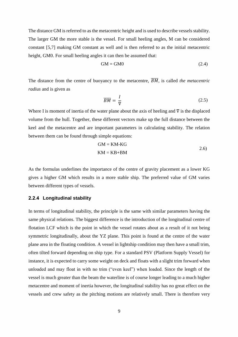
The distance GM is referred to as the metacentric height and is used to describe vessels stability.
The larger GM the more stable is the vessel. For small heeling angles, M can be considered
constant [5,7] making GM constant as well and is then referred to as the initial metacentric
height, GM0. For small heeling angles it can then be assumed that:
GM = GM0 (2.4)
The distance from the centre of buoyancy to the metacentre, 𝐵𝑀̅̅ ̅̅ ̅, is called the metacentric
radius and is given as
𝐵𝑀̅̅ ̅̅̅ = 𝐼
∇ (2.5)
Where I is moment of inertia of the water plane about the axis of heeling and ∇ is the displaced
volume from the hull. Together, these different vectors make up the full distance between the
keel and the metacentre and are important parameters in calculating stability. The relation
between them can be found through simple equations:
GM = KM-KG 2.6)
KM = KB+BM
As the formulas underlines the importance of the centre of gravity placement as a lower KG
gives a higher GM which results in a more stable ship. The preferred value of GM varies
between different types of vessels.
Longitudinal stability
In terms of longitudinal stability, the principle is the same with similar parameters having the
same physical relations. The biggest difference is the introduction of the longitudinal centre of
flotation LCF which is the point in which the vessel rotates about as a result of it not being
symmetric longitudinally, about the YZ plane. This point is found at the centre of the water
plane area in the floating condition. A vessel in lightship condition may then have a small trim,
often tilted forward depending on ship type. For a standard PSV (Platform Supply Vessel) for
instance, it is expected to carry some weight on deck and floats with a slight trim forward when
unloaded and may float in with no trim (“even keel”) when loaded. Since the length of the
vessel is much greater than the beam the waterline is of course longer leading to a much higher
metacentre and moment of inertia however, the longitudinal stability has no great effect on the
vessels and crew safety as the pitching motions are relatively small. There is therefore very

10
unlikely that a vessel will capsize as a result of the trimming moment. Figure 2.5 shows a simple
drawing of a trimming vessel.
Figure 2.5 A vessel in a trimming condition, trimming forward
2.3 Vessel response
In this chapter some basic theory about ship movements relevant to this project will be
explained.
Response in regular waves
When a vessel encounters a wave it will be displaced in one or several directions depending on
the direction of the wave. For regular waves the elevation of this wave can be defined as [8]
𝜁 = 𝜁𝑎sin(𝜔𝑡) (2.7)
where 𝜁𝑎 is the amplitude of the wave and 𝜔 is the wave frequency.
In any given reference point on the vessel, i.e. the LCG, there will be a displacement as a
reaction to the vessel encountering the wave. This displacement will be slightly different from
the wave elevation and the relation between these two can be described by response amplitude
operators (RAO) or mathematically Transfer functions given as

11
𝜂𝑘(𝑡) = 𝜂𝑘𝑎 cos(𝜔𝑡 + 𝜃𝑘) , 𝑘 = 1, … ,6. (2.8)
where 𝜂𝑘𝑎 is the motion amplitude per unit wave amplitude and 𝜃 is the phase angle1.
Strip Theory
The principles of Strip Theory, or 2D Potential Theory makes it possible to determine forces
and motions on a three-dimensional floating body by considering the body being made up of
several two-dimensional sections, or strips, which in all together make up the whole shape of
the hull. According to [5], each of these sections can be considered treated as a section of a
floating, infinitive cylinder with a linear boundary problem and hydrodynamic effects
calculated and solved for each of them. This is visualized in Figure 2.6.
Figure 2.6 Strip theory.[6]
2.4 Stability criteria
After the Bourbon Dolphin incident, a commissions from the NMD came up with several
proposals to prevent similar accidents from happening. In this chapter the new and current
stability criteria will be presented and briefly explained.
1 The phase angle tells the phase relationship, or timing between the vessels motion relative to the wave. i.e. a
phase angle of +-180 degrees means response is opposite of the wave elevation and 0 degrees means that those
two are in phase [8]

12
General stability criteria
In the DNVGL rules and standards documents [9], the following requirements apply for all
vessels above 24 m:
“The area under the righting lever curve (GZ curve) shall not be less than 0.055 metre-
radians up to θ = 30° angle of heel and not less than 0.09 metre-radians up to θ = 40° or
the angle of flooding θf if this angle is less than 40°. Additionally, the area under the
righting lever curve between the angles of heel of 30° and 40° or between 30° and θf, if
this angle is less than 40°, shall not be less than 0.03 metre radians”
“The righting lever (GZ) shall be at least 0.20 m at an angle of heel equal to or greater
than 30°.”
“The maximum righting lever should occur at an angle of heel preferably exceeding 30°
but not less than 25°”
“The initial metacentric height, GM0 shall not be less than 0.15 m.”
Special criteria for AHTS
In the proposed regulations the NMD address the importance of doing the necessary
calculations for vessels used for anchor handling involving use of towing winch to show both
acceptable and the critical conditions for “vertical and horizontal transverse force/tension and
as a minimum include the following [9,10]:
When affected by the maximum acceptable tension in the wire/chain including the maximum
transverse force/tension, the maximum acceptable heeling angle should be limited to one of the
following angles that occurs the first:
15° degrees heeling angle.
The flooding angle, which means green water emerging on the deck.
Angle equal to 50 % of maximum GZ
They recommend that the heeling moment and righting arm are to be considered from the upper
and outer edge of the stern roller when the tension force is to be calculated. The key angles and
parameters is presented in Figure 2.7 and Figure 2.8.

13
Ft
v
Figure 2.7 Back view of vessel
Ft is the tension force in the mooring line and v is the vertical distance of the horizontal force
component relative to the centre of thrust and y is the horizontal distance of the mooring line
relative to the vessels centre line.
Figure 2.8 Side and top view of vessel
Mooring forces
As the mooring line is often subject to great tension force and acting from varying angles it is
considered a critical factor when it comes to the stability of an AHV. The force acting in the
mooring line is more dynamic rather than static and varies by the amount of wire released and
environmental forces such as waves and current. As mentioned the line of attack from the
mooring line may vary and affect the ship in several ways, most notably by heel and trim. The

14
ship will also experience being pulled backwards which means extra requirements when it
comes to bollard pull. Figure 2.9 shows a vessel seen from starboard (XZ-plane) showing the
force components from the mooring line.
αXZ
X
Z
Figure 2.9 Side view of force components from the mooring setup
The total force from the mooring line in the three dimensional space is found as
𝐹𝑀𝐿,𝑋𝑌𝑍 = 𝐹𝑀𝐿 (2.9)
Which can be decomposed into the horizontal and vertical force components
𝐹𝑀𝐿,𝑋𝑌 = 𝐹𝑀𝐿 sin(𝛼𝑋𝑍) (2.10)
𝐹𝑀𝐿,𝑍 = 𝐹𝑀𝐿 cos(𝛼𝑋𝑍) (2.11)
Where 𝛼𝑋𝑍 is the angle between the direction of the total force and the vertical force component
in the XZ-plane.
Figure 2.10 shows the vessel seen from above and the force components are now considered in
the XY-plane. For this explanation the force components are somewhat simplified as there are
other factors contributing to the final angle of attack of the force, such as the changing angle of
the mooring line at the starboard stopping pin. Friction is also neglected in the calculations so
there is no force on the stern roller.

15
Figure 2.10 Aft end of a vessel with the force components
So based on the equations 2.9-2.11 in the previous section, the new force components are found
as
𝐹𝑀𝐿,𝑋 = 𝐹𝑀𝐿,𝑋𝑌 cos(𝛽𝑋𝑍) = 𝐹𝑀𝐿 sin(𝛼𝑋𝑍) cos(𝛽𝑋𝑍) (2.12)
𝐹𝑀𝐿,𝑌 = 𝐹𝑀𝐿,𝑋𝑌 sin(𝛽𝑋𝑌) = 𝐹𝑀𝐿 sin(𝛼𝑋𝑍) sin(𝛽𝑋𝑌) (2.13)
The distance y from the centre line and the force is a vital parameter when considering the effect
from the mooring line as it will create a rotational moment on the vessel. The force FML,Z is
acting downwards on the stern roller with a distance XAFT from G and has a distance YSR from
the centre line. The distance is found by
𝑌𝑆𝑅 = 𝑋𝑇𝑃 tan(𝛽𝑋𝑌) + 𝑌𝑇𝑃 (2.14)
Where 𝛽 is considered equal to the rotation of the ship, yaw-angle. If the angle of attack from
the winch is considered small there will only be one force component acting from the winch,
acting in x-direction towards the stern. The sum of forces then makes this force equal to 𝐹𝑀𝐿,𝑋.
As there are no considerable force components acting from the winch in y-direction, the sum
of forces then gives
𝐹𝑀𝐿,𝑌 = 𝐹3 (2.15)

16

17
3 Modelling approach
In this chapter the software used in the project is presented and process of dimensioning and
modelling the barge is explained.
3.1 Software
AquaSim
AquaSim is a time-domain Finite Element Analysis-tool developed by Trondheim based
Aquastructures AS. The software is aimed at both stiff and flexible marine constructions subject
to static and dynamic loads from winds, waves, currents etc. In AquaSim one can execute time
simulations and investigate the interaction between stiff and flexible elements of different types
and typical cases are operations involving mooring, towing and heavy lifting. AquaSim consist
of the current modules which are used in this project:
- AquaEdit – Creating geometric models [11]
- AquaBase – Define material and hydrodynamic properties to the models [12]
- AquaSim solver – Derive results from AquaBase from time domain simulations [13]
- AquaView – Shows the results in 3D [14]
The models made in AquaSim can consist of different element types such as Beam and Truss
which are used in this project. The elements are modelled as simple lines between to two nodes
and then given the necessary properties. Beam elements are as the name suggests structural
objects such as beams and bars which can be subject to bending stress. Truss elements are used
to define objects used for mooring such as ropes, chains and others. These elements are given
pre-defined or custom properties regarding mechanical attributes, cross-section, material, load
parameters depending on what is to modelled.
ShipX Vessel Reponses Program
ShipX VERES is a software developed by MARINTEK to calculate and analyse ship motions
and global loads for aid in the design process of ships. The program uses linear, potential, Strip
Theory to calculate the hydrodynamic loads on any given hull. The hull is imported or created
in the program and is defined by several sections resembling its shape. Input is given regarding
ship geometry, loading condition, velocity and wave direction which is used by the Main
Program to calculate the transfer functions for the ship motions and loads. For making reports,
plot results for presentation, the Postprocessor will execute this and do further calculations. For
more information, see [8,16].

18
3.2 Barge model
Geometry and hydrostatics
For investigating the dynamic effects that a mooring line has on a AHTS one has to set up a
realistic scenario with all the necessary elements involved in an anchor-handling operation. Due
to limitations in the software a less complex model has to be used thus a barge with similar
dimensions were chosen. A simple barge is modelled in AquaSim and compared with an
identical model in ShipX and used for the analysis. The main dimensions of the barge are
chosen to replicate similar sized offshore-vessels and can be found in below.
L
T B
D
X
Z
Y
Figure 3.1 Components of a modelled Barge in AquaSim
As a barge is can be considered more or less as a rectangular box, its initial stability can be
found by simple formulas by using either weight or draft as constant.
Due to its shape a barge will have a block coefficient2, Cb close or equal to 1 and
To find the GM of the barge one must know the components that it consists of which is governed
by the shape and mechanical attributes where we have the relation mentioned in equation 2.5
𝐵𝑀 = 𝐼
∇
Which 𝐼 for a boxed-shape barge is found as
𝐼 =𝐵3𝐿
12 (3.1)
2 The Block Coefficient 𝐶𝐵 is the ratio between the displaced volume divided by 𝐵𝑊𝐿 𝑥 𝐿𝑊𝐿 𝑥 𝑡. The latter
parameters define a box around the submerged body of the vessel which the block coefficient shows how much is
“occupied” by the displaced volume.

19
Which shows the importance of the breadth is for the initial stability. Furthermore, the displaced
volume is defined as
∇= 𝐵𝐿𝑡 (3.2)
From this the weight ∆ can be found by multiplying the volume with the water density 𝜌 and
the other way around for finding the volume if the weight is known. The properties of a box-
shaped Barge of considerable size makes it very stable in water as it has a GM much higher
than what is found on vessels with more hydrodynamic shape. Based on the formulas explained
earlier, the main dimensions are chosen with respect to the GM. The dimensions are presented
in Table 3.1
Table 3.1 Barge geometry and hydrostatics
Parameter Abbr. Value
Length L 80 [m]
Breadth b 18 [m]
Depth D 8 [m]
Draught t 5 [m]
VCG - 6 [m]
GMt - 1.9 [m]
Natural roll period
When analysing the motions of a vessel some awareness of the natural period is necessary. The
natural period can in this case be defined as the period in which the vessel oscillates. When a
wave approaches with a period close to the natural period of the vessel the response can increase
dramatically. In a plot of RAO data, the natural period can be identified where the peak of the
curve is. To make accurate predictions of the natural period for all the vessels motions, stiffness
and mass effects from the vessel floating should be included, such as added mass3. According
to [17] an estimate can be done for the natural roll period in air, excluding added mass:
𝑇𝑟𝑜𝑙𝑙_𝑎𝑖𝑟 = 2𝜋 ∗ √𝑟44
2
𝐺𝑀̅̅̅̅�̅� ∗ 𝑔
(3.3)
Where 𝑟44 roll radius of gyration which for a barge is set as the breadth divided by four.
For the barge with the given dimensions and 𝐺𝑀̅̅̅̅̅𝑇 the natural roll period can be estimates as
3 Added inertia due to the vessel accelerating and displacing water as it moves through it. Different for each
motion(DOF)

20
𝑇𝑟𝑜𝑙𝑙_𝑎𝑖𝑟 = 2𝜋 ∗ √4.5𝑚2
1.9𝑚 ∗ 9.81 𝑚𝑠2⁄
= 6.55𝑠
3.3 Modelling in AquaSim
This chapter presents the modelling procedure of the barge and mooring line. These models
consist of beam and truss elements respectively and are defined by the given properties:
Properties to the mechanical properties of an element
Properties related to the cross section
Properties related to how elements respond to loads
The given properties for the models can be found in Appendix A.
Load calculation
In AquaSim there are two load definitions that can be applied to the given elements;
Hydrodynamic load and Morison submerged load definition. With Hydrodynamic load, linear
strip theory is used as described earlier in this report. This is typically used for floating elements
like a barge in this case.
Morison load definition is applied to submerged elements with small diameter relative to the
wave length and is used for calculating loads from current and waves acting on threads, cables
and anchor lines [18]. The equation is implemented in AquaSim as following:
𝐹2 =𝜌𝑤 𝐶𝑑𝑦𝐷𝑖𝑎𝑚𝑁𝐿0
2(𝑢2 − �̇�2𝑚)√(𝑢2 − �̇�2𝑚)2(𝑢3 − �̇�3𝑚)2
+𝜌𝑤(1 + 𝐶𝑎𝑦)𝑉2𝐷𝐿0𝑎2 − 𝜌𝑤𝐶𝑎𝑦𝑉2𝐷𝐿0�̈�2
(3.4)
Where 𝐶𝑑𝑦 is the drag coefficient in local y-direction, 𝐷𝑖𝑎𝑚𝑁 is the diameter of the cross-
section in the direction of the relative velocity √(𝑢2 − �̇�2𝑚)2(𝑢3 − �̇�3𝑚)2 vector in the cross-
sectional plane. 𝑢2 is the combination of fluid velocity due to waves(𝑢2𝑤𝑎𝑣𝑒) + current velocity
in the local y-direction(𝑢2𝑐𝑢𝑟𝑟𝑒𝑛𝑡), �̇�2𝑚 is the velocity at the element mid point in local y-
direction, 𝑎2 is the fluid acceleration in local y-direction, (1 + 𝐶𝑎𝑦) is the mass coefficient with
𝐶𝑎𝑦 being the added mass coefficient. As presented the equation consists of three parts:
- The first part of this equation is the drag part

21
- The second is the Froude Kryloff4 part and diffraction part of the load
- The third part is the added mass
The force component in z-direction is calculated in a similar way.
Procedure
When modelling a barge for mooring analysis in AquaSim, a specific procedure is used
according to [19] which is explained in this chapter. This procedure shows that the barge
consists of several parts; Main beam element, a 2D hydrodynamic beam element and so called
“Dummies” for mooring points. The assembly of these elements is shown in Figure 3.2.
Figure 3.2 Components of a modelled Barge in AquaSim
Both the main element and 2D hydrodynamic element are defined as “hydrodynamic elements”
which means that the hydrodynamic loads is calculated by linear strip theory. Drift forces are
also chosen for these two elements and is defined as [18]:
𝐹𝑑𝑟𝑖𝑓𝑡 = 𝜌𝑔
2∗ 𝐴𝑟
2 (4.4)
Where 𝐴𝑟 is the amplitude of the reflected wave. For regular waves this is a constant force
Main element
The main beam element is modelled with the length of the barge with a cross-section
representing the rest of the barge as shown in Figure 3.3. As the element is modelled in the
4 The Froude–Krylov force does, together with the diffraction force, make up the total non-viscous forces acting
on a floating body in regular waves. The diffraction force is due to the floating body disturbing the waves

22
water line the coordinates represents how the barge is floating in water, with the negative Z-
coordinate representing the draft and the positive representing the freeboard.
Figure 3.3 Cross section for Main element
2D-Hydrodynamic element
The 2D hydrodynamic beam element is modelled perpendicular to and across the middle of the
main beam with the length equal to the width of the main beam and width equal to the length
of the main beam. Figure 3.4 presents the cross section of this element.
Figure 3.4 Cross section for 2D hydrodynamic element
The “2D Hydrodynamic, horizontal loads only” is checked for this element. This means that
only the horizontal components of the hydrostatic and hydrodynamic forces are considered and
is done to make the barge able to handle waves from all directions within one analysis model
[21]. This element will therefore not add buoyancy to the model.
Dummies
The “Dummies” are modelled as beam elements with mooring points but without visual cross-
section data and volume and defined with Morison load.

23
Environmental loads
The environmental loads, is given as “Normal”, where directions are based on the global
coordinate system [21]. All of the weather parameters are chosen in the same menu as shown
in Figure 3.5. Each line represents a load condition run with the chosen loads. These parameters
are as presented in Table 3.2
Table 3.2 Weather loads and description
Property Unit Description
Nr. - Order of the load condition
Amp m Wave amplitude
T Sec Wave period in seconds
V deg. Wave direction from global positive x direction
c(x) m/s Current velocity in x-direction
c(y) m/s Current velocity in y-direction
w(x) m/s Wind velocity in x-direction
w(y) m/s Wind velocity in y-direction
Comment - Description of the load condition
Group - Group number if several analyses are to be executed
The environmental loads menu is as presented in Figure 3.5. Different conditions can be set
with varying wave periods
Figure 3.5 Weather loads as presented in AquaBase
Properties for the time domain simulations
The time series analysis is set up in AquaBase as presented in Table 3.3. A pre-increment of 5
seconds is chosen as default and basically means that the environmental loads will build up in
steps from 0 to the given value during the first 5 seconds into the simulation. If the current is
set to 1 m/s then it will be 0 at step 1, 0.2 at step 2 etc. until it reaches 1 at step 5. The number
of maximum iterations is set to the upper limit of 10000 to avoid diverging and make sure that
the results are valid. The number of time steps set for one wave is set to a minimum of 12
seconds with a total number of steps set to 360, meaning there will be simulated a total of 30

24
waves after the incremented time. The number of total steps is varied between some load
conditions due to either convergence problems or the fact that for some load conditions the
amplitudes took longer or shorter time to stabilize. The wave profile is set as -1 meaning that
the formula for infinite water depth is used. A positive number means the formula for finite
depth is used [21].
Table 3.3 Time series setup in AquaBase
Time series
Pre-increment 5
Max iterations per step 10000
No. Total steps for waves 360
No. Steps for one wave 12
Convergence criteria 1
Depth (wave profile) -1
Barge constraints
As explained in the motion chapter a free floating vessel has 6 degrees of freedom as it can
translate and rotate freely along and about the x-, y- and z-axis. Assigning DOF’s to a model
can be challenging as it is not always clear which nodes should be locked, and to what degree,
to get the realistic behaviour of the model. The barge consists mainly of a longitudinal and
transverse element which creates a natural set of end nodes and an intersecting point in the
middle, which for the barge is also G. Two additional nodes are added with constraints to
simulate thrusters counteracting the rotational moment from the mooring line. The idea is also
that potential thrust forces from these can be read from these nodes. The complete DOF-
configuration is presented in Figure 3.6. The end-nodes of the 2D-hydrodynamic element had
to be locked for x-translation and z-rotation as there where some issues with the model splitting
up after a certain amount of simulation time. This is elaborated further in the discussion-chapter.

25
[0,1,1,1,1,0]
[0,1,1,1,1,0]
[0,0,1,1,1,0]
[1,1,1,1,1,0]
[1,1,1,1,1,0]
[1,1,1,1,1,1]
[1,1,1,1,1,1]
Figure 3.6 DOF in nodes on Barge model. 1=free 0=locked
Mooring line model
The mooring line is modelled as truss-elements in AquaSim. Material data is based on
approximate values from a technical report about the offshore semi-sub Eirik Raude[21],
various product sheets [22] and from the commission report from NMD[8]. Table 3.4-3.5
presents the parameters given for the anchor line and work wire respectively.
Table 3.4 parameters for anchor line
Diameter Material Weight in air Weight in water Total length No. elements
84 mm Steel 150 kg/m 146.7 kg/m 3500 m 600
Table 3.5 parameters for work wire
Diameter Material Weight in air Weight in water Total length No. elements
48 mm Steel 25kg/m 23 kg/m 340 m 112
Offshore installations are often moored with a combination of chain and wire to reduce weight
of the total configuration. The chain can also consist of several different elements and
connections. AquaSim allows this configuration to be as realistic as possible as it is just a matter
of material input. The configuration presented in the tables above is a simplified one.
The loads on the mooring line is calculated by Morison load definition.
3.4 Modelling in ShipX
The barge is modelled in ShipX by defining simple stations and contour lines [16]to create the
overall shape of the hull. The cross-sections are defined in a coordinate-system with x-direction

26
being positive forward. When sections and contours are defined the hull geometry is presented
as shown in Figure 3.7. Due to the simple shape of the barge, only 5 sections is made.
Figure 3.7 Drawing of hull geometry as presented in ShipX
The load condition is defined where draught and length and breadth of waterline is set according
to what is given AquaSim. A Vessel Response Calculation is then defined where the vessel
description and condition info is set. In the vessel description, metacentric heights, mass, VCG,
LCG and radii of gyration is defined to match the data given in AquaSim. The hydrodynamic
loads are calculated by using linear strip theory.

27
4 Case studies
A set of case studies is performed to analyse the barge and mooring line. In this chapter they
are presented. They are defined to expose the influence of the mooring line on the barges
response in different conditions and loads.
4.1 Case study descriptions
Case study 1 purpose
The purpose of this case study is to get an overview of the vessel response in the initial phase
of receiving the mooring line.
Case study 2 purpose
The purpose of this study is to investigate and evaluate the effects of having the approximately
full length of the mooring chain trailing from the stern
Case study 3 purpose
With the same position as in case 2, the purpose of this study is to investigate and evaluate the
vessel response after the anchor is dropped from the stern hanging from the working line and
anchor chain.
For case 1-3 the mooring line is centred. A visual presentation of these cases can be seen in
Figure 4.1.
Case study 4 purpose
The purpose of this study is to investigate how the behaviour of the vessel changes when the
mooring line is acting outside the centreline and with a varying angle. This case consists of the
two conditions presented in Figure 4.2
4.2 Waves and current
A set of waves with defined wave periods, amplitude, heading and current is set in the program
for each case study. For time saving and expected relevancy based on the plots in Figure 5.1,
only wave periods(T) from 6-9 seconds are considered. For the cases where current is included
this is set to 1m/s.

28
Figure 4.1 Simple study cases of AH operation involving OI and AHV
Figure 4.2 Loading conditions for study case 4. Mooring line set at 60 and 36 degrees’ angle of attack

29
5 Simulation and results
This chapter presents the results from the time domain simulations done. From here the study
cases will be referred to as Case #1, Case #2 and Case #3 with Case #0 being the barge without
mooring line and deck load. In the results chapter only the most necessary plots will be shown
as other results are enclosed in the appendix.
The simulations are performed with waves approaching from different directions, in this case 0
and 90 degrees known as head- and beam sea respectively. Depending on the direction of the
waves different motions will be more or less occurring. In this project only the most critical
motions will be considered and Table 5.1 shows when each of them are considered and the
units:
Table 5.1 Wave headings and acting motions
Term Direction [deg] Heave[m] Roll[deg] Pitch [deg]
Head Sea 0 X X
Beam Sea 90 X X (X)5
The mooring line force is found as “Axial force” in AquaSim and is presented as such in the
plots.
5.1 Verification of movements
To verify the dynamic movements of the model and make sure that the values can be taken
directly from the analysis the analysis is done both in AquaSim and ShipX for comparison.
ShipX is a renowned program for calculating ship response and similar motions between the
programs will confirm the legitimacy of the results in AquaSim. This is done by running a
“vessel response” in ShipX for the barge model and a simulation in AquaSim. The values in
AquaSim are found from reading the maximum, stabilized values for rotation and displacement
for the given wave headings and periods with the measurements done from the CoG.
In ShipX, these values are plotted automatically as a function of wave period.
Comments on result
Figure 5.1 presents the RAO data from AquaSim and ShipX. The graphs show good
correspondence between the programs except for roll. The roll motion found from AquaSim is
5 Pitch motion will be considered when the barge is affected by the mooring line

30
peaking at about 6.5 seconds as predicted in the barge model chapter. In the same section it is
also mentioned that this is a very simple estimation of the natural roll period without the
inclusion of proper viscous effects which are included in the ShipX calculations.
(a) Heave and Roll motion in beam sea
(b) Pitch and Heave motion in head sea
Figure 5.1 Heave, roll and pitch comparison
0
0,5
1
1,5
2
4 5 6 7 8 9 10 11 12
T [s]
Heave[m]
AquaSim ShipX
0
5
10
15
20
4 5 6 7 8 9 10 11 12
T [s]
Roll [deg]
AquaSim ShipX
0
0,5
1
1,5
2
2,5
4 5 6 7 8 9 10 11 12
T [s]
Pitch [deg]
AquaSim ShipX
0
0,2
0,4
0,6
0,8
1
4 5 6 7 8 9 10 11 12
T [s]
Heave [m]
AquaSim ShipX

31
5.2 Study Case 1 – AHV close to OI
Simulation setup
Head- and beam waves are considered with no current. The mooring line is attached and centred
at the stern. The vessel is placed 340m from the OI with the total length of the mooring line at
525m with its lowest point at 200m, leaving the stern with an angle of 40 degrees. The anchor
is considered resting the stern.
Comments on results
Some of the results from the simulation are presented in Figures 5.2-5.4. The barge is
considered at the shortest distance from the imagined rig and therefore the mooring line is at its
shortest length. This situation is reflected in the figures as there are no significant changes in
the vessel motions other than what is expected for roll motion around T=6.5s. Figure 5.2(a)
shows that the addition of the mooring line induce a small static angle in regard of pitch motion
in head sea. In this case that angle is measured to be -0.2 degrees, meaning that the vessel is
operating with a slight negative trim. The largest pitch motion in head sea is found at T=9s
seconds as indicated in Figure 5.1 (b).
Figure 5.2(b) and (c) shows the roll motion for the barge in beam sea. The graph indicates that
the addition of the mooring line has a reduction effect on the roll motion at T=6.5s despite that
the mooring line is acting in the centre line of the barge. This effect is most notably at T=6.5s
which is close to the natural roll period of the barge which can give bigger changes in the
amplitude. In Figure 5.3 the time series for pitch motion for beam sea is presented and shows
that the motion in beam seas is peaking at around 200 seconds before decreasing compared to
pitch motion in head sea which stabilized after 50 seconds.
Figure 5.4 presents the axial force in the mooring line is presented which is the force acting on
the stern of the barge. As the figures shows the force at this point is not significantly high,
varying from 330 kN at the lowest and 470 kN at the highest, with the biggest variations close
to the natural roll period. For T=4 the force is close to the median of around 400 kN.

32
(a) Pitch motion at T=6.5(left) and T=9(right). Head sea
(b) Roll motion for T=6.5. Beam sea
(c) Roll motion for T=7s. Beam sea
Figure 5.2 Case #0 and #1 Comparison of pitch and roll motion at T=6.5s and T=7s.
-0,6
-0,4
-0,2
0
0,2
0,4
0 20 40 60 80
Ro
tati
on
[d
eg]
Time [s]
Case #0 Case #1
-2,5-2
-1,5-1
-0,50
0,51
1,52
2,5
0 10 20 30 40 50 60 70 80 90
Ro
tati
on
[d
eg]
Time [s]
Case #0 Case #1
-20
-10
0
10
20
500 510 520 530 540 550 560 570 580 590 600
Ro
tati
on
[d
eg]
Time [s]
Case #0 Case #1
-18
-12
-6
0
6
12
18
0 100 200 300 400 500
Ro
tati
on
[d
eg]
Time [s]
Case #0 Case #1
-12
-6
0
6
12
570 580 590 600
Ro
tati
on
[d
eg]
Time [s]Case #0 Case #1

33
Figure 5.3 Case #1. Pitch motion for T=6.5s and 7s seconds in beam sea.
Figure 5.4 Case #1. Axial force in mooring line acting on the stern in beam sea.
-1,5
-1
-0,5
0
0,5
1
0 100 200 300 400 500 600
Ro
tati
on
[de
g]
Time [s]
T=6.5 T=7
320
370
420
470
0 20 40 60 80 100 120
Axi
al f
orc
e [
kN]
Time [s]
T=6.5 T=7

34
5.3 Study Case 2 – At drop point
Simulation setup
In this case study the vessel is placed about 3250m from the IO with the total length of the
mooring line at approximately 3500m with the lowest point at 650m depth. In addition to the
previously used environmental loads, the effect of current is also considered.
Comments on result
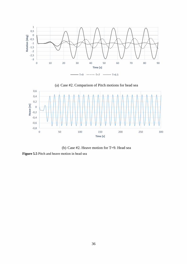
Figure 5.5 presents the heave and pitch motions in head sea. Figure 5.5(a) and shows the pitch
motion for a selection of wave periods where the largest amplitude occurs at T=9s with 2
degrees. Overall the amplitudes stabilize early and an increased static angle forces the vessel
into a negative initial trim of -1 degree. Figure 5.5(b) shows the highest measured heave motion
which is found at T=9s for both case #1 and #2. The graph shows that the mooring line has
caused the draught of the barge to increase by 0.12m at midship.
Figure 5.6 presents the roll-, pitch-motion and mooring line force in beam sea. Figure 5.6(a)
shows the roll motion measured at T=6.5s and 7s. The results show that the increased length of
the mooring line has increased roll motion and moved the peak from 6.5 seconds to 7 seconds.
The roll motion for 6.5 seconds is now decreased by almost a third compared to Figure 5.2(a).
Figure 5.6 (b) shows the pitch motion for T=6.5s and 7s. Judged by the variations in the time
series the plots indicates that there is a connection between the pitch motion and roll motion.
The added force from the mooring line has increased the static angle and the barge now has an
initial trim of -1 degree, compared to -0.2 in Case #1.
Figure 5.6(c) Presents the mooring line force at T=6.5s and 7s. As with the roll and pitch
motion, the peak of the force just before 200 seconds. The amplitudes are then varying in a
pulsating pattern. Figure 5.7 presents a comparison of the roll-, pitch-motion and mooring line
force for wave amplitudes 1m and 2m. Figure 5.7(a) presents the roll motion at T=6.5s and
shows that the roll motion for 2m wave amplitude is much larger and has some larger variations
in the beginning but is identical with 1m wave amplitude from 300 seconds and further. Figure
5.7(b) presents the pitch motion at T=6.5s with varying wave amplitudes and shows that
increasing the wave amplitude from 1m to 2m causes bigger variation in the pitch motion. The
average pitch value also seems to shift over time. Figure 5.7(c) presents the mooring line force
which has now also increased.

35
Figure 5.8 presents the roll motion and mooring line forces influenced by varying wave
amplitude and current. Figure 5.8(a) shows that the addition of current has reduced the overall
roll motion for both amplitudes and periods. For T=7s with 2m wave amplitude the average
value increases rapidly and may indicate that the model is becoming too unstable.
Figure 5.8(b) shows the mooring line force for T=6.5s influenced by current and varying wave
amplitude. As with the roll and pitch motions it has been reduced.
36
(a) Case #2. Comparison of Pitch motions for head sea
(b) Case #2. Heave motion for T=9. Head sea
Figure 5.5 Pitch and heave motion in head sea
-3
-2,5
-2
-1,5
-1
-0,5
0
0,5
1
0 10 20 30 40 50 60 70 80 90
Ro
tati
on
[d
eg]
Time [s]
T=9 T=7 T=6.5
-0,8
-0,6
-0,4
-0,2
0
0,2
0,4
0,6
0 50 100 150 200 250 300
He
ave
[m
]
Time [s]

37
(a) Case #2. Comparison of roll motion at T=6.5s(left) and 7s(right). Beam sea
(b) Case #2. Comparison of pitch motion at T=6.5s(left) and 7s(right). Beam sea
(c) Case #2. Comparance of force in mooring line at T=6.5s(left) and 7s(right). Beam sea
Figure 5.6 Case #2. Roll-, pitch-motion and mooring line force at T=6.5s and 7s. Beam sea
-15
-10
-5
0
5
10
15
0 200 400 600
Ro
tati
on
[d
eg]
Time [s]
-25-20-15-10
-505
10152025
0 200 400 600
Rta
tio
n [
de
g]
Time [s]
-1,5
-1,3
-1,1
-0,9
-0,7
-0,5
0 200 400 600
Ro
tati
on
[d
eg]
Time [s]
-1,7
-1,5
-1,3
-1,1
-0,9
-0,7
-0,5
0 200 400 600
Ro
tati
on
[d
eg]
Time [s]
2750
2800
2850
2900
0 200 400 600
Axi
al f
orc
e [
kN]
Time [s]
2750
2800
2850
2900
0 200 400 600
Axi
al f
orc
e [
kN]
Time [s]

38
(a) Case #2. Roll motion for T=6.5s, with amplitude 1m and 2m. Beam sea
(b) Case #2. Pitch motion for T=6.5s with amplitude 1m and 2m. Beam sea
(c) Case #2. Mooring line force at T=6.5s with amplitude 1m and 2m. Beam sea
Figure 5.7 Roll motion with amplitude 1 and 2. Case #2
-20
-10
0
10
20
0 100 200 300 400 500 600
Ro
tati
on
[d
eg]
Time [s]
Amp = 2 Amp = 1
-2
-1,5
-1
-0,5
0
0 100 200 300 400 500 600
Ro
tati
on
[d
eg]
Time [s]Amp = 2 Amp = 1
2600
2700
2800
2900
3000
0 100 200 300 400 500 600
Axi
al f
orc
e [
kN]
Time [s]
Amp = 2 Amp = 1

39
(a) Case #2. Roll motion for T=6.5s(left) and 7s(right) for amplitude 1m and 2m with current = 1m/s
(b) Case #2. Comparison between mooring line force at T= 6.5s with current = 1 m/s. Amplitude
1m and 2m
Figure 5.8 Roll motion and mooring line force with varying amplitudes and with current.
-10
-8
-6
-4
-2
0
2
4
6
8
10
0 200 400 600
Ro
tati
on
[d
eg]
Time [s]
Amp = 1 Amp=2
-25
-20
-15
-10
-5
0
5
10
15
20
25
0 200 400 600
Ro
tati
on
[d
eg]
Time [s]
Amp = 1 Amp=2
2750
2775
2800
2825
2850
2875
2900
0 100 200 300 400 500 600
Amp=1 Amp=2

40
5.4 Study Case 3 – Anchor in water
Simulation setup
Vessel positioned as in Case #2 but with the anchor now hanging from the stern at about 340m
depth. Previous environmental loads apply.
Comments on results
Figure 5.9 presents the pitch and heave motion in head sea. Figure 5.9(a) presents the pitch
motion for T=9s and indicates that moving the anchor from the stern roller into the water does
not affect the pitch significantly compared to Case #2. Figure 5.9(b) presents highest measured
heave motion which is measured at T=9s. There is no significant difference in amplitude
compared to Case #2.
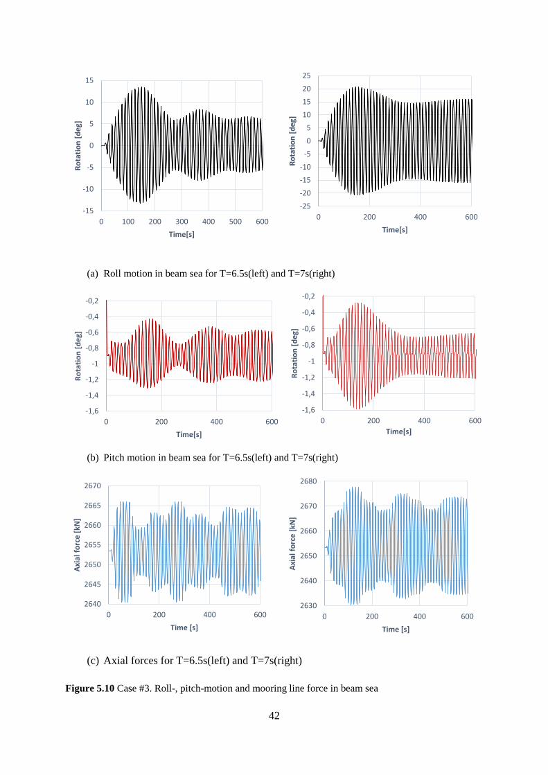
Figure 5.10 presents roll-, pitch-motion and mooring line force at T=6.5s and 7s. Overall the
roll- and pitch-motions are similar to what seen in case #2 but with some reduced values. Figure
5.10(c) presents the mooring line at T=6.5s and 7s. The figure is showing that the average
mooring line forces for T=6.5s and 7s have decreased from 2833 kN to 2653 kN and the time
series are more unstable compared to case #2.

41
(a) Pitch motion for T=6.5s, 7s and 9s. Head sea
(b) Heave motion for T=9s. Head sea
Figure 5.9 Case #3. Pitch and Heave motions in head sea
-3,5
-3
-2,5
-2
-1,5
-1
-0,5
0
0,5
1
1,5
0 20 40 60 80 100 120
Ro
tati
on
[d
eg]
Time [s]
6.5 7 9
-0,8
-0,6
-0,4
-0,2
0
0,2
0,4
0,6
0 20 40 60 80 100 120
He
ave
[m
]
Time [s]
42
(a) Roll motion in beam sea for T=6.5s(left) and T=7s(right)
(b) Pitch motion in beam sea for T=6.5s(left) and T=7s(right)
(c) Axial forces for T=6.5s(left) and T=7s(right)
Figure 5.10 Case #3. Roll-, pitch-motion and mooring line force in beam sea
-15
-10
-5
0
5
10
15
0 100 200 300 400 500 600
Ro
tati
on
[d
eg]
Time[s]
-25
-20
-15
-10
-5
0
5
10
15
20
25
0 200 400 600
Ro
tati
on
[d
eg]
Time[s]
-1,6
-1,4
-1,2
-1
-0,8
-0,6
-0,4
-0,2
0 200 400 600
Ro
tati
on
[d
eg]
Time[s]
-1,6
-1,4
-1,2
-1
-0,8
-0,6
-0,4
-0,2
0 200 400 600
Ro
tati
on
[d
eg]
Time[s]
2640
2645
2650
2655
2660
2665
2670
0 200 400 600
Axi
al f
orc
e [
kN]
Time [s]
2630
2640
2650
2660
2670
2680
0 200 400 600
Axi
al f
orc
e [
kN]
Time [s]

43
5.5 Case study 4 – Angled line with offset from centre
Simulation setup
This case is based on case 2 with the only difference being the change in direction of the
mooring line. Two conditions are simulated with the mooring line pulling the vessel from 60°
and 36°(relative to the YZ-plane).
Comments on result
Figure 5.11 presents the roll- and pitch motion with variation in mooring line angle. Figure
5.11(a)(b) shows the roll motion for T=9s and 7s with 60° and 36° angle on the mooring line.
The graph shows that there is a minor difference in the static angle from 60° and 36° and that
the mooring line in 60° angle is inducing higher amplitudes compared to 36° for both periods.
5.11(c) Shows the pitch motion for T=7s with variation in mooring line angle. There is not
much difference between the two variations but most noticeably is that the time series are more
unstable and the amplitudes are varying irregularly. As the trendlines are indicating, the average
pitch motion is increasing which means that the barge is unstable, at least for the simulated
period.
Figure 5.12 presents a summary of roll motion measured in the study cases. It shows how the
peak period of the roll motion is moving from T=6.5s to 7s as a result of the mooring line
configuration changing. It is clear that the increased length of the mooring line and the change
in position has a negative effect on the roll motion.

44
(a) Roll motion for T= 9s. Beam sea
(b) Roll motion for T=7s. Beam sea
(c) Pitch motion for T=7s. Beam sea
Figure 5.11 Case #4. Roll- and pitch-motion with varying angle on mooring line and 1.8m offset from
barge centre line.
-8
-4
0
4
8
12
0 50 100 150 200 250 300
Ro
tati
on
[d
eg]
Time [s]
Mooring line 60° Mooring line 36°
-15
-10
-5
0
5
10
15
20
0 50 100 150 200 250 300
Ro
tati
on
[d
eg]
Time [s]Mooring line 60° Mooring line 36°
-1,1
-1
-0,9
-0,8
-0,7
-0,6
-0,5
-0,4
0 200 400 600
Ro
tati
on
[d
eg]
Time [s]Mooring line 36°
-1,2
-1,1
-1
-0,9
-0,8
-0,7
-0,6
-0,5
-0,4
0 200 400 600
Ro
tati
on
[d
eg]
Time [s]Mooring line 60°

45
Figure 5.12 Comparison of roll motion for all study cases based on wave period.
0
5
10
15
20
25
6 6,5 7 7,5 8 8,5 9
Ro
tati
on
[d
eg]
T [s]
No load Case #1 Case #2 Case #3 36° angle 60° angle

46
47
6 Discussion
6.1 Software
The AquaSim package consists of several modules as mentioned which aims to aid through the
whole analysis process and proves to be a versatile software for mooring analyses. For this
project however, there were some complications when setting up the analysis. It seems like the
main strength of the program is mooring analysis with non-free floating constructions moored
in several directions compared to a free floating vessel with a mooring line attached to it.
6.2 Barge simplifications
The initial plan was to use a simple barge model while getting to know the software and later
use a more realistic model of an AHV for the analysis and motion verifications however, it
proved difficult to get a realistic ship model implemented into the software as it would require
several elements each with individual input. An attempt was done to make more complex hull
but due to the amount of input needed and general uncertainty about the functionality of the
model at that time the idea was abandoned. It was decided that the barge would be the test
vessel for the simulation and it was dimensioned to resemble a larger offshore vessel.
The modelling of the barge was done according to a user manual provided by Aquastructures
which explained step by step how a barge should be modelled. The barge in the manual where
about half the size of the one used in the project. There were some issues regarding the moment
of inertia as the analysis would not run with the given input. By recommendation from
Aquastructures the default values from the manual were used.
In the early stages of the simulation there were some problems with the analysis as it was unable
to converge for certain cases. When investigating the case in the AquaView module it showed
that the barge model started to lose its stiffness and split up after a certain amount of simulation
time. This could be due to the modelling technique used not being meant for barges at this size
and that the input given does not correspond to its physical size.
6.3 Constraints
Due to the issues regarding convergence and the analysis not starting the model was given extra
constraints. Initially it was just locked in G for x- and y-translation to avoid it drifting away.
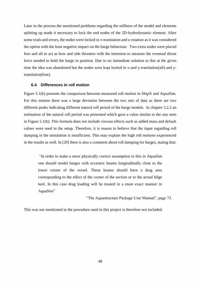
48
Later in the process the mentioned problems regarding the stiffness of the model and elements
splitting up made it necessary to lock the end nodes of the 2D-hydrodynamic element. After
some trials and errors, the nodes were locked in x-translation and z-rotation as it was considered
the option with the least negative impact on the barge behaviour. Two extra nodes were placed
fore and aft to act as bow and side thrusters with the intension to measure the eventual thrust
force needed to hold the barge in position. Due to no immediate solution to this at the given
time the idea was abandoned but the nodes were kept locked in x-and y-translation(aft) and y-
translation(fore).
6.4 Differences in roll motion
Figure 5.1(b) presents the comparison between measured roll motion in ShipX and AquaSim.
For this motion there was a large deviation between the two sets of data as there are two
different peaks indicating different natural roll period of the barge models. In chapter 3.2.2 an
estimation of the natural roll period was presented which gave a value similar to the one seen
in Figure 5.1(b). This formula does not include viscous effects such as added mass and default
values were used in the setup. Therefore, it is reason to believe that the input regarding roll
damping in the simulation is insufficient. This may explain the high roll motions experienced
in the results as well. In [20] there is also a comment about roll damping for barges, stating that:
“In order to make a more physically correct assumption to this in AquaSim
one should model barges with eccentric beams longitudinally close to the
lower corner of the vessel. These beams should have a drag area
corresponding to the effect of the corner of the section or to the actual bilge
keel. In this case drag loading will be treated in a more exact manner in
AquaSim”
“The Aquastructure Package User Manual”, page 73.
This was not mentioned in the procedure used in this project is therefore not included.

49
6.5 Results
The main results are already commented before every study case but some reflection is needed.
The overall impression is that there are some clear connections between the time series
however, this varied a lot between wave periods and not all results were stable and kept
increasing as the time simulation time went on.
The model used in the analysis was far from optimal as constraints and simplifications were
done to get it to work. There is reason to believe that these measures affected the results. Based
on the results and previous comments it is clear that especially the results found for roll motion
should be considered invalid when considering periods close to the natural roll period.
In case #1 the barge was subject to the least amount of force as the mooring line was relatively
short. Some minor changes in static angles for trim was registered and slight changes in roll
amplitude but the variations were the same. In Case #2 the mooring line was at its longest hence
the larger forces and thereby larger responses. Figure 5.10 indicate that roll and heave follows
the same pattern for each wave period while there were no clear connections with the variation
of mooring line forces. The exception may be that it is evident that by increasing the
environmental loads, mainly increasing wave amplitude and adding current induced multiple
variations in all responses(Figure 5.8) which seemed to follow the same pattern. There were no
significant changes in case #3.
In case #4 the mooring line was placed outside the centre line of the barge, more specifically
1.8m and with the mooring line angle in two different angles. These angles were somewhat
randomly chosen. Most interesting here is that the mooring line in an 60° angle is inducing both
higher roll- and pitch-motion compared to 36° and that the roll motion is reduced for both
angles. One explanation of this can be that the forces from the mooring line at the smaller angle
is inducing a yaw-motion rather than roll and pitch compared to the larger angle. and that the
offset of 1.8m is the main factor. Combined with the constraints that locks the barges yaw
motion, the change in angle of the mooring line may limit the barges roll motion.
When comparing the cases for roll motion, it is clear that the length and position of the mooring
line has a negative effect on the roll motion.

50

51
7 Conclusion and future work
7.1 Conclusion
A final model resembling a barge with a mooring chain and working line have been modelled
and simulated in AquaSim for some specific load cases. From these, data describing the motions
of the barge and force acting on it from the mooring line were extracted.
The main field of use for AquaSim is mooring analysis of different kinds which the interface
of the program reflected. This made it rather easy to model a relatively complex mooring setup
with different types of chain and wires, given the right input. Still, the models used in this
project can be considered somewhat simplified as not all parameters were clearly defined and
thus given default values.
The barge model has some critical limitations. One of them is the mechanical properties which
required input of different moments of inertia however, when calculating them for the barge
with respect to its size the simulation often encountered convergence issues. As a solution to
this, default values were used, based on recommendations from some of the developers of the
program. As these values represented a much smaller barge, the mechanical properties used are
not correct. This became evident when the model was compared with an identical model in
ShipX, as the RAO’s were more or less identical except for the roll motion. The deviation
increased for higher roll amplitudes and should therefore be considered invalid for certain wave
periods.
The modelling technique used to create the barge can be questioned as some of the convergence
issues that were encountered came as a result of the models tendency to split after a certain
amount of simulation time. From the look of it, it seemed like the model split at points where
the elements were divided by nodes, basically dividing the main element and hydrodynamic
element into two rectangles each. Similar issues were identified when measuring pitch motions
as there were signs of the barge not being rigid enough longitudinally, causing and inconsistent
rotational movement about y-axis.
Study cases were set up and analysed to investigate the mooring lines effect of the barge
response under varying environmental loads. The simulations show that the barge is subject to

52
great amount of force from the mooring line, with varying differences of up to 200 kN found
for specific conditions. This mostly due to the increased length of the mooring line and the
change in angle and position of the line. The results also indicate that worse sea conditions
through increased wave height and current increase the forces acting on the barge and making
the response more varying.
7.2 Future work
A more realistic ship model should be implemented or the model technique for the barge
should be altered as the size seems to cause some problems. Eventual changes could
include the part quoted in the discussion section regarding roll damping. The input
regarding this should be more adjusted to the given analysis.
Without having too much knowledge about the software, the analysis may be more
suitable together with the stability software AquaStab, especially when it comes to
analysing the stability regarding rules and criteria.
A more sophisticated mooring line configuration should be made and cases involving
seabed interaction might be interesting to investigate as the software is capable of this.
Analysis involving waves approaching from 45 degrees should be investigated as it is
highly relevant and induces coupled motions.

53
REFERENCES
[1] NOU, Norges offentlige utredninger, “Bourbon Dolphins forlis den 12. april 2007.”
(2008)
[2] M. Hancox and H. Clarkson, “Anchor Handling” (2011).
[3] www.skipsmedia.no/island-vanguard (C.Tussøy)(01.06.2016)
[4] www.rolls-royce.com (20.05.16)
[5] J. Journée and W. Massie, “Offshore hydromechanics” (2000).
[6] K. Koskinen “ Numerical simulation of ship motion due to waves and
manoeuvring”.(2012)
[7] A. Biran and R. L. Pulido, “Ship hydrostatics and stability.” (2013).
[8] MARINTEK AS, “ShipX Vessel Responses (VERES) User’s Manual” (2015).
[9] DNV GL “rules for classification for ships Pt. 3 Ch. 15 Sec. 1,” (2015)
[10] Sjøfartsdirektoratet, "Rapport om tiltak for ankerhåndteringsfartøy og flyttbare
innretninger." (10.02.2009)
[11] Aquastructures AS, “AquaEdit user manual”. (2016)
[12] Aquastructures AS, “AquaBase user manual”. (2016)
[13] Aquastructures AS, “AquaTool user manual”. (2016)
[14] Aquastructures AS, “AquaView user manual”. (2016)
[15] G. Ritchie, “Practical introduction to anchor handling and supply vessel operations”
(2007)
[16] MARINTEK AS, “ShipX Workbench Getting Started,” (2004).
[17] S. Fjelde. ”Stability and motion response analyses of transport with barge.” (2008)
[18] J.A. Berstad,”Theoretical formulation of structure and load modelling, Report no.2006-
301”(2006)
[19] Aquastructures AS, “Brukermanual AquaSim Fortøyningsanalyse av fórflåter,” (2016).
[20] Aquastructures AS, “The AquaSim Package User Manual”. (2014)
[21] Inocean AS, “Eirik Raude Semi-Submersible Drilling Unit, Calculation of Mooring
System.” (2005)
[22] ].G. Maritime, “Anchor manual 2015 the guide to anchoring.” (2015)


APPENDIX A – Model input In this appendix is the material data for the elements in the Barge assembly.
Main element:
Material/section properties for Main beam
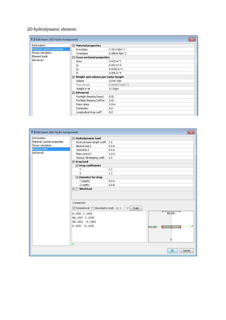
2D hydrodynamic element:

Working line

Anchor line


APPENDIX B – CD Content of the attached CD-rom:
Full thesis and article draft in PDF-format
Excel spreadsheet with time series
Models used for all study cases(5)


APPENDIX C – Article draft

1
APPENDIX C – Article draft
Investigation of tensile forces in anchor lines and influence on
vessel behaviour [Article draft]
Petter Langeland (M.Sc Ship Design) Email: [email protected]
ABSTRACT
This paper is based on a master’s thesis where case
studies where done to investigate the effects of
mooring line on vessel response using time-domain
analysis. The model is resembling a barge and is,
together with a mooring line configuration, modelled
in AquaSim [1], a time domain FEA (Finite Element
Analysis) software developed by Aquastructures AS.
A part of the project was to check how suitable the
software is for this kind of analysis. The paper focus
on how the variation in mooring line length,
direction and position and acting tensile force affect
the vessel in regard of heave-, -roll and pitch-motion.
In the analysis the model is under subject to varying
loads from the mooring line, waves and current.
The works shows that the mooring line and barge are
subjects to large variations in force and motions and
that there are some connections between the tensile
force and roll and pitch motion.
AquaSim shows great versatility when it comes to
mooring-related analyses, with the aquaculture
industry as one of its biggest users. As it is claimed
that is capable of performing dynamic analysis of
vessel motion there are some limitations regarding
the model as it was, at the current point, not possible
to implement a realistic hull to analyse. RAO data
from MARINTEK vessel response software ShipX
but the prescribed motions could not be influenced
by the mooring line. As a result, a barge was chosen
as test model.
INTRODUCTION
Anchor Handling is one of the most complex
operations done by offshore ships in the North Sea
as it demands a lot from both crew and vessel. Under
operation the vessel is affected by a number of
different forces varying in both size and direction
which puts high strain on stability as well as
affecting the structure and equipment. In April 2007
the AHTS vessel “Bourbon Dolphin” capsized while
deploying an anchor for the semi-submersible rig
“Transocean Rather” 75 nautical miles northwest
from Shetland, resulting in the death of 7 people. The
commission set up for the investigation highlighted
several factors that contributed to the capsizing but
in the end it was the loss of stability that caused
it[2,3]. As a result of this the Norwegian Maritime
Directorate proposed several changes in rules and
standards to be implemented in the design process
and operation of AHTS vessels to prevent similar
situations to happen again.
This master thesis aims to give an overview of how
these forces affects the stability under operation.
Figure 1 Bourbon Dolphin
Anchor Handling Vessels(AHV)
are multi-utility vessels which are mainly built to
handle anchors and performing towing operations.
These operations are often related to oil rigs where
towing them to their location to anchor them up are
some of the main tasks however, they are also used
to transport supplies between offshore installations
and mainland as well as support in emergency
situations at sea and performing ROV-services. Due
to the nature of an AHTS vessels work, there are high
requirements when it comes to manoeuvrability,
stability, and pulling power/Bollard pull. The vessel
design is characteristic and with a steering house,
and winch house in front of a large deck area with
barriers on the side to protect the crew and
equipment. The stern is open and enforced with a
stern roller to handle chains grinding on the edge.
Further explanation of the equipment is found later
in this chapter. The length can vary from 50 metre to
well over 100 m with a width of 15-25 metres.
Bollard pull can vary from 60 tonnes on the smallest
ones to over 400 tonnes on the bigger and most
advanced ships

2
AHV operations
Anchor handling operations are in this project
divided into two rough phases; deployment and
recovering of anchors. Deployment of the anchor is
often done by the vessel towing the anchor line from
the rig to a given position. At the position the anchor
is connected and lowered into the ocean using the
working line from the winch. The weather condition
is critical as the AHV is already exposed to large
forces from the anchor line, depending on the length
of the line. To handle the addition of waves, current
and side winds it is critical for the vessel to have
enough stability. The recovery of the anchor is more
or less the reverse process of deploying it. The AHV
drag the anchor loose from the seabed and starts to
winch up the anchor and simultaneously reversing as
the rig pulls the mooring line [4]
Vessel response (RAO)
When a vessel encounters a wave it will be displaced
in one or several directions depending on the
direction of the wave. For regular waves the
elevation of this wave can be defined as [3]
𝜁 = 𝜁𝑎sin(𝜔𝑡) where 𝜁𝑎 is the amplitude of the wave and 𝜔 is the
wave frequency.
In any given reference point on the vessel, i.e. the
LCG, there will be a displacement as a reaction to
the vessel encountering the wave. This displacement
will be slightly different from the wave elevation and
the relation between these two can be described by
response amplitude operators (RAO) or
mathematically Transfer functions given as
𝜂𝑘(𝑡) = 𝜂𝑘𝑎 cos(𝜔𝑡 + 𝜃𝑘) , 𝑘 = 1, … ,6.
where 𝜂𝑘𝑎 is the motion amplitude per unit wave
amplitude and 𝜃 is the phase angle.
The hydrodynamic loads are calculated by linear
strip theory in both AquaSim and ShipX. This is
done by considering the floating body being made up
of several two-dimensional sections, or strips, which
in all together make up the whole shape of the hull.
According to [5], each of these sections can be
considered treated as a section of a floating,
infinitive cylinder with a linear boundary problem
and hydrodynamic effects calculated and solved for
each of them. For the elements with this load
definition, diffraction and radiation forces from
waves are taken into account.
Load calculations
In the program the barge is defined for
hydrodynamic loads which means that linear strip
theory is used to calculate the loads as described
in[6].
For the mooring line, Morison load calculations will
be used as defined in[6]
𝐹2 =𝜌𝑤 𝐶𝑑𝑦𝐷𝑖𝑎𝑚𝑁𝐿0
2(𝑢2 − �̇�2𝑚)
*√(𝑢2 − �̇�2𝑚)2(𝑢3 − �̇�3𝑚)2
+𝜌𝑤(1 + 𝐶𝑎𝑦)𝑉2𝐷𝐿0𝑎2 − 𝜌𝑤𝐶𝑎𝑦𝑉2𝐷𝐿0�̈�2
BARGE MODEL
Geometry
The properties of a box-shaped Barge of
considerable size makes it very stable in water as it
has a GM much higher than what is found on vessels
with more hydrodynamic shape. Based on hand-
calculations, the main dimensions are chosen with
respect to the GM which was aimed to be around 1.5-
1.9. The dimensions are presented in table 1.
Parameter Abbr. Value
Length L 80 [m]
Breadth B 18 [m]
Depth D 8 [m]
Draught T 5 [m]
VCG - 6 [m]
GMt - 1.9 [m]
Table 1
RESULTS
Motion verification
To verify the dynamic movements of the model and
make sure that the values can be taken directly from
the analysis the analysis is done both in AquaSim
and ShipX for comparison. ShipX is a renowned
program for calculating ship response and similar
motions between the programs will confirm the
legitimacy of the results in AquaSim. This is done by
running a “vessel response” in ShipX for the barge
model and a simulation in AquaSim. The values in
AquaSim are found from reading the stabilized
values for rotation and displacement for the given
wave headings with the measurements done from the
CoG. The simulations are performed with waves
approaching from different directions, in this case 0
and 90 degrees known as head- and beam sea
respectively
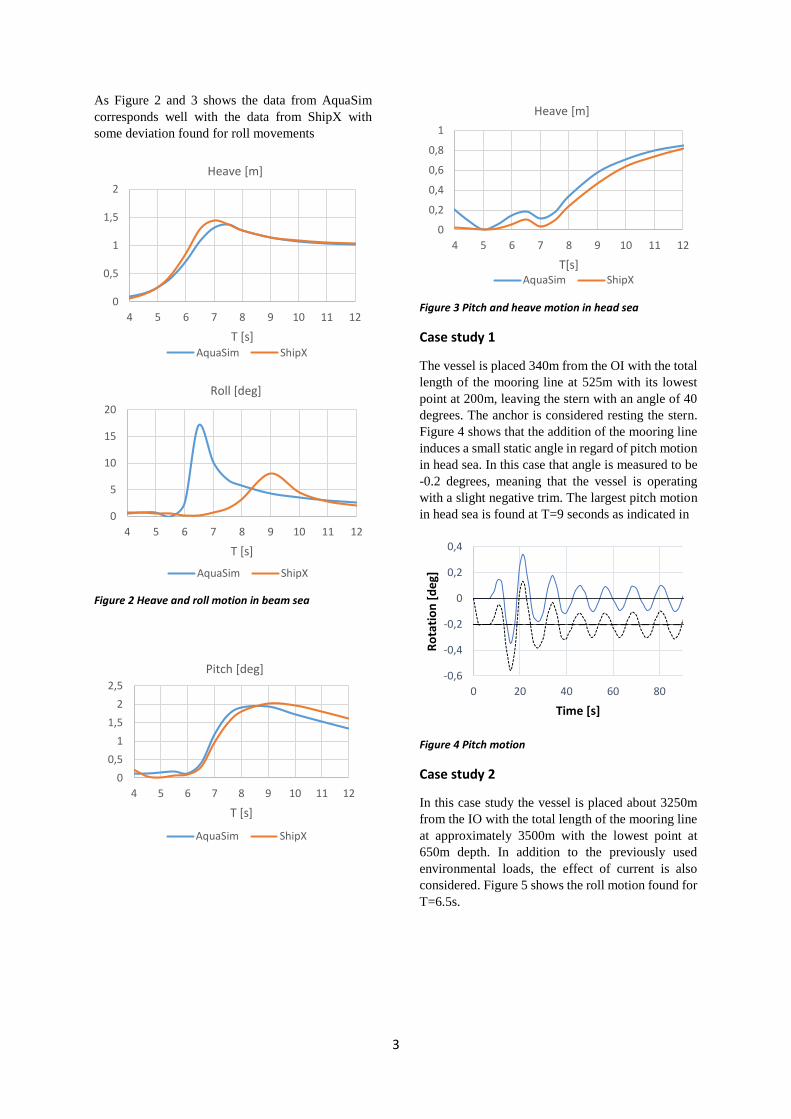
3
As Figure 2 and 3 shows the data from AquaSim
corresponds well with the data from ShipX with
some deviation found for roll movements
Figure 2 Heave and roll motion in beam sea
Figure 3 Pitch and heave motion in head sea
Case study 1
The vessel is placed 340m from the OI with the total
length of the mooring line at 525m with its lowest
point at 200m, leaving the stern with an angle of 40
degrees. The anchor is considered resting the stern.
Figure 4 shows that the addition of the mooring line
induces a small static angle in regard of pitch motion
in head sea. In this case that angle is measured to be
-0.2 degrees, meaning that the vessel is operating
with a slight negative trim. The largest pitch motion
in head sea is found at T=9 seconds as indicated in
Figure 4 Pitch motion
Case study 2
In this case study the vessel is placed about 3250m
from the IO with the total length of the mooring line
at approximately 3500m with the lowest point at
650m depth. In addition to the previously used
environmental loads, the effect of current is also
considered. Figure 5 shows the roll motion found for
T=6.5s.
0
0,5
1
1,5
2
4 5 6 7 8 9 10 11 12
T [s]
Heave [m]
AquaSim ShipX
0
5
10
15
20
4 5 6 7 8 9 10 11 12
T [s]
Roll [deg]
AquaSim ShipX
0
0,5
1
1,5
2
2,5
4 5 6 7 8 9 10 11 12
T [s]
Pitch [deg]
AquaSim ShipX
0
0,2
0,4
0,6
0,8
1
4 5 6 7 8 9 10 11 12
T[s]
Heave [m]
AquaSim ShipX
-0,6
-0,4
-0,2
0
0,2
0,4
0 20 40 60 80
Ro
tati
on
[d
eg]
Time [s]

4
Figure 5 Roll motion for T=6.5s
When comparing roll and pitch motion, some
similarities could be seen as the peaks occurs at
approximately the same time. Figure 6 presents the
pitch motion found for T=6.5 seconds.
Figure 6 Pitch motion for T=6.5s
Figure 7 presents the mooring line force at T=6.5s.
As with the roll and pitch motion, the peak of the
force just before 200 seconds. The amplitudes are
then varying in a pulsating pattern. Figure 8 shows
the same series with varying wave amplitude which
shows that there is much more instability.
Figure 7 Axial force for T=6.5s
Figure 8 Axial force with wave amplitude 1m and 2m.
Case study 3
Vessel positioned as in Case #2 but with the anchor
now hanging from the stern at about 340m depth.
Previous environmental loads apply. There were no
significant changes in vessel response from case #2
to #3.
Figure 9 Study Case #3
Figure 12 presents the measured roll motions for the
different cases. The figure shows that the peak of the
roll period is increasing from 6.5 seconds in case #0
and #1 to 7 seconds for case #2, #3 and #4.
Case study 4
A fourth study case was analysed with the mooring
line leaving the stern at varying angles, namely 60
and 36 degrees. An offset of 1.8m from the barge
centre line was also set. Figure 10 presents a
summary of all the cases. It shows that the natural
roll period of the barge has shifted from 6.5 seconds
to 7 seconds which is expected as the extra load is
affecting the barges range of motion.
-15
-10
-5
0
5
10
15
0 200 400 600
Ro
tati
on
[d
eg]
Time [s]
-1,5
-1,3
-1,1
-0,9
-0,7
-0,5
0 200 400 600
Ro
tati
on
[d
eg]
Time [s]
2750
2800
2850
2900
0 200 400 600
Axi
al f
orc
e [
kN]
Time [s]
2750
2800
2850
2900
0 200 400 600
Axi
al f
orc
e [
kN]
Time [s]
Amp=1 Amp=2

5
Figure 10 Roll motion for different cases
Figure 11 presents the axial forces measured for case
#2 and #3. The figure indicates that, as expected, the
highest force is found in case #2 where the mooring
line is longer however, the addition of current[1m/s]
does not change the force noticeably. In case #3
where the anchor is dropped in the ocean, the force
has decreased with about 200 kN. This is most likely
due to the force being measured in a different
material, as it is now the work wire that pulls in the
barge.
Figure 11 Axial forces from different cases
CONCLUSION
A final model resembling a barge with a mooring
chain and working line have been modelled and
simulated in AquaSim for some specific load cases.
The software has some limitations which is why a
barge was used.
The barge was analysed in both AquaSim and ShipX
where the comparison shows that there are some
differences in the analysis setup as there is a large
deviation in roll motion.
Study cases were set up and analysed to investigate
the mooring lines effect of the barge response under
varying environmental loads. The simulations show
that the barge is subject to great amount of forces
from the mooring line, with varying differences of
up to 200 kN found for specific conditions. Added
loads such as current and increased wave height
made the forces and response more unpredictable.
REFERENCES
[1] Aquastructures AS, “The AquaSim Package User Manual”. (2014)
[2] NOU, Norges offentlige utredninger, “Bourbon Dolphins forlis den 12. april 2007.” (2008)
[3] Sjøfartsdirektoratet, "Rapport om tiltak for ankerhåndteringsfartøy og flyttbare
innretninger." (10.02.2009)
[4] M. Hancox and H. Clarkson, “Anchor Handling” (2011).
[5] MARINTEK AS, “ShipX Vessel Responses (VERES) User’s Manual” (2015).
[6] J.A. Berstad, ”Theoretical formulation of structure and load modelling, Report no.2006-301”(2006)
0
5
10
15
20
25
6 7 8 9
Ro
tati
on
[d
eg]
T [s]
No load Case #1
Case #2 Case #3
36° angle 60° angle
2550
2650
2750
2850
2950
4 5 6 7 8 9
Axi
al f
orc
e [
kN]
T [s]Case 2 Case 3 Case 2 w/current