investigation of energized options for leachate …

INVESTIGATION OF ENERGIZED OPTIONS FOR LEACHATE MANAGEMENT:

Photochemical iron-mediated aeration treatment of landfill leachate

November 2006

Daniel E. Meeroff François Gasnier

C.T. Tsai

Florida Atlantic University

State University System of Florida Florida Center for Solid and Hazardous Waste Management

University of Florida 2207-D NW 13th Street Gainesville, FL 32609 www.floridacenter.org

Report # 0632018

ii

INVESTIGATION OF ENERGIZED OPTIONS FOR LEACHATE

MANAGEMENT:

Photochemical iron-mediated aeration treatment of landfill leachate

Daniel E. Meeroff Florida Atlantic University

Boca Raton, FL, 33431 561-297-3099

François Gasnier Florida Atlantic University

Boca Raton, FL, 33431 561-297-2830

C.T. Tsai Florida Atlantic University

Boca Raton, FL, 33431 561-297-2824

Final Report Year 1 for the

William W. "Bill" Hinkley

Center for Solid and Hazardous Waste Management

NOVEMBER 2006

iii

ACKNOWLEDGEMENTS

The research was sponsored in part by the William W. "Bill" Hinkley Center for Solid and Hazardous Waste Management and Florida Atlantic University. Joe Lurix, John Booth, Ray Schauer, Shaowei Chen, C.T. Tsai, Richard Meyers, Fred Bloetscher, Manuel Hernandez, Marc Bruner, Matt Zuccaro, Lee Casey, J.P. Listick, and Bill Forrest are thanked for sharing their input as members of the Technical Advisory Group. The following individuals are thanked for their contributions to the research: Tim Vinson, John Schert, Deng Yang, William Koseldt, and Jim Englehardt.

iv

ABSTRACT

Author: François Gasnier

Title: Photochemical iron-mediated aeration treatment of landfill

leachate

Institution: Florida Atlantic University

Principal Investigator: Dr. Daniel Meeroff

Year: 2006

Municipal landfill leachate is a high strength wastewater containing high levels of COD, TDS, ammonia and eventually high BOD5 and other toxics. Treatment of leachate is becoming more of an issue as regulations tighten and wastewater treatment plants reduce their accetance of leachate. Several treatment techniques are currently available. The first objective is to establish an outline of these techniques and rank the alternatives according to efficiency, cost and environmental sustainability. This list should not be limited to current practice. Relatively uncommon approaches, i.e. advanced oxidation processes and energized processes seem to show the most promising results in the literature. Thus photochemical iron-mediated aeration (an energized process) will also be tested, first on simulated leachate and then on real leachate from the Solid Waste Authority of Palm Beach County. A laboratory scale Photochemical Iron Mediated Aeration (PIMA) reactor was designed and tested for five components (COD, BOD5, ammonia, TDS and conductivity). Results are encouraging but are expected to be improved during subsequent testing with real leachate.

v

EXECUTIVE SUMMARY

This report describes the results of the first year of a proposed two-year study of energized options for leachate management. Objectives The objective of the proposed two-year study was to develop two new energized processes for leachate treatment and assess their sustainability (performance, risk, and cost) comparatively to the currently available treatment alternatives. Specifically, objective one was to examine the literature on energized alternatives for detoxification and treatment of leachate; collect leachate quality data; identify issues/trends associated with long-term leachate management; and prepare a list of energized alternatives ranked according to environmental sustainability, efficiency, risk, and economic factors. During this first year, leachate has been characterized, treatment techniques are under study. Objective two of the proposed study was to design and test laboratory reactors for leachate treatment using energized options such as the photochemical iron-mediated aeration technology (PIMA) and TiO2-magnetite photocatalytic processes. During the first year of this project, only the PIMA process has been investigated. Objective 3 was to prepare preliminary cost analyses and risk assessments on selected technologies to provide a Florida-specific matrix of engineering alternatives that are innovative, economical, and environmentally sound to aid solid waste management personnel in decision-making. Rationale Municipal landfill leachate is a high strength wastewater characterized by high concentrations of recalcitrant organic compounds, ammonia and, metals. As such, leachate is difficult to treat biologically or chemically. Additionally, because of widely varying practices in solid waste management across the state of Florida, an understanding of emerging issues and an inclusive solution to long-term management of landfill leachate is currently not available. Currently, leachate is mainly discharge to the sewer system. But stricter regulations and more and more reluctant wastewater treatment plant are forcing to find other solutions. This research will address these needs and produce a valuable decision-making tool for solid waste managers. The research will also generate performance data to develop unit treatment costs for scale-up and address current barriers to the use of futuristic technologies for reducing toxic loads in water, wastewater, and soils in addition to leachate. Methods This study was divided into four distinct but overlapping tasks. The first task was to establish the list of the existing technologies and examine their respective efficiencies and costs. During this process, leachate was also characterized in quality

vi

as well as in quantity. Resources such as the FAU S.E. Wimberley Library services (Electronic databases such as FirstSearch or WorldCat and Electronic journals), Internet (reliable sources such as government or universities web sites: www.epa.gov, www.dep.state.fl.us), record review at the FDEP of Palm Beach were used. Also, the Technical Advisory Group was very helpful to specifically center this task on Florida. Task two was dedicated to the design of the PIMA and TiO2-magnetite photocatalysis reactors. The Photochemical Iron-Mediated Aeration process reactor design is based on the development made by Meeroff et al. (2006). The TiO2-magnetite photocatalysis reactor is under development at this time. The testing of the process was executed in task three. Components tested are: ammonia, BOD5, COD, dissolved solids, conductivity and heavy metals. This step was divided into three subtasks. In the first one, the influent leachate was made up using a solution of a unique component. In the second subtask, the influent was a made up mixture of these components. And finally, the processes were tested on real leachate, collected from the Solid Waste Authority of Palm Beach County. At this time, lead is the only component that has not been studied on the first subtask of the PIMA process. The final task was to compare the PIMA and TiO2-magnetite catalysis processes with other viable technologies. During the development of the process, the most efficient parameters will be found. Based on these pilot scale reactors and results from real leachate, a capital and an operational and maintenance cost will be estimated for the two processes. A ranking of the technologies will be established as a function of removal efficiency, cost per gallon of treated leachate and environmental risk. This task is currently not started. Conclusions Based on the literature review conducted, it appears that many different options are available to treat leachate. These options are municipal sewer discharge without pretreatment, natural evaporation pond, deep well injection, hauling off-site, leachate recirculation or bioreactor, on-site treatment which can be biological processes such as activated sludge systems, waste equalization ponds, aerated lagoons, trickling filters, rotating biological contactors, or anaerobic digesters or physical and chemical processes such as coagulation, flocculation, precipitation and sedimentation, carbon adsorption, ion exchange, air stripping, filtration. Of these alternatives, none is showing good treatment efficiency without producing more dangerous residuals. Another area of treatment method is the advanced oxidation processes and energized processes. Such processes are hydrogen peroxide, Fenton (H2O2/Fe2+), ozone, ozone and hydrogen peroxide, ultraviolet light, Photo-Fenton / Fenton-like systems, ultraviolet light and hydrogen peroxide, ultraviolet light and ozone, ultraviolet light, ozone and hydrogen peroxide, photocatalytic oxidation such as the Iron-Mediated Aeration (IMA), the PIMA and the UV/TiO2 catalysis. This

vii

second category seems to achieve a better treatment while producing less harmful residuals. The literature review also permitted to establish the composition of a typical leachate. The main parameters are ammonia, BOD5, COD, conductivity, TDS and heavy metals. At this time, scoping tests concerning ammonia, BOD5, COD, conductivity and TDS have been performed using the PIMA process. The results obtained are conform to the expectations. Ammonia is not removed by the air stripping because of the acidic pH. Concerning conductivity and TDS, the removal is counter balanced by the dissolution of iron in solution. But concerning COD and BOD5, the PIMA process showed better removal results than the IMA and UV control processes. But these results are expected to improve when using real leachate.

viii

KEY WORDS landfill leachate, photochemical, iron-mediated, aeration, COD, BOD5, lead, ammonia, conductivity, TDS

ix

TABLE OF CONTENTS

ACKNOWLEDGEMENTS......................................................................................... iii ABSTRACT................................................................................................................. iv EXECUTIVE SUMMARY .......................................................................................... v KEY WORDS............................................................................................................ viii LIST OF TABLES....................................................................................................... xi LIST OF FIGURES ................................................................................................... xiii LIST OF ABREVIATIONS AND NOTATIONS..................................................... xiv Chapter 1: Introduction and Literature Review ........................................................- 2 -

1.A. Municipal Solid Waste Management ............................................................- 3 - 1.A.1. Generation and disposal .........................................................................- 3 - 1.A.2. Landfill, definition and construction......................................................- 5 -

1.B. Leachate ........................................................................................................- 8 - 1.B.1. Definition ...............................................................................................- 8 - 1.B.2. Typical composition.............................................................................- 10 -

1.C. Treatment options........................................................................................- 14 - 1.C.1. Municipal sewer discharge without pretreatment ................................- 14 - 1.C.2. Evaporation ..........................................................................................- 15 - 1.C.3. Deep well injection...............................................................................- 15 - 1.C.4. Hauling off-site ....................................................................................- 16 - 1.C.5. Leachate recirculation: bioreactor........................................................- 16 - 1.C.6. On-site treatment ..................................................................................- 17 -

1.C.6.a. Biological processes ......................................................................- 17 - 1.C.6.b. Physical and chemical processes...................................................- 18 -

1.C.7. Alternative treatment methods: AOPs and EPs....................................- 20 - 1.C.7.a. Hydrogen peroxide ........................................................................- 22 - 1.C.7.b. Fenton (H2O2/Fe2+)........................................................................- 22 - 1.C.7.c. Ozone.............................................................................................- 23 - 1.C.7.d. Ozone and hydrogen peroxide.......................................................- 23 - 1.C.7.e. Ultraviolet light .............................................................................- 24 - 1.C.7.f. Photo-Fenton / Fenton-like systems ..............................................- 24 - 1.C.7.g. Ultraviolet light and hydrogen peroxide .......................................- 24 - 1.C.7.h. Ultraviolet light and ozone............................................................- 25 - 1.C.7.i. Ultraviolet light, ozone and hydrogen peroxide.............................- 25 - 1.C.7.j. Photocatalytic oxidation.................................................................- 25 - 1.C.7.k. Iron-Mediated Aeration (IMA) .....................................................- 26 - 1.C.7.l. Photochemical Iron-Mediated Aeration (PIMA) ...........................- 27 -

1.C.8. Ranking of treatment options ...............................................................- 27 - 1.D. Problem statement.......................................................................................- 27 - 1.E. Objectives ....................................................................................................- 28 -

Chapter 2: Methodology .........................................................................................- 30 - 2.A. Reactor design and construction .................................................................- 31 -

x

2.B. Experimental protocol .................................................................................- 37 - 2.B.1. Simulated leachate................................................................................- 37 - 2.B.2. Real leachate ........................................................................................- 39 -

2.C. Parameters ...................................................................................................- 39 - 2.C.1. Hydraulic retention time.......................................................................- 39 - 2.C.2. Distance (UV radiation) .......................................................................- 39 - 2.C.3. Iron fibers .............................................................................................- 40 - 2.C.4. Mixing and aeration conditions............................................................- 41 - 2.C.5. Filtration ...............................................................................................- 42 -

Chapter 3: Results and discussion...........................................................................- 44 - 3.A. Simulated leachate: individual scoping tests ..............................................- 45 -

3.A.1. COD .....................................................................................................- 45 - 3.A.1.a. Low concentration level ................................................................- 45 - 3.A.1.b. Medium concentration level..........................................................- 46 - 3.A.1.c. High concentration level ...............................................................- 47 - 3.A.1.d. Summary .......................................................................................- 47 -

3.A.2. Conductivity and TDS .........................................................................- 48 - 3.A.2.a. Low concentration level ................................................................- 48 - 3.A.2.b. Medium concentration level..........................................................- 50 - 3.A.2.c. High concentration level ...............................................................- 52 - 3.A.2.d. Summary .......................................................................................- 53 -

3.A.3. BOD5....................................................................................................- 54 - 3.A.3.a. Low concentration level ................................................................- 54 - 3.A.3.b. Medium concentration level..........................................................- 55 - 3.A.3.c. High concentration level ...............................................................- 55 - 3.A.3.d. Summary .......................................................................................- 56 -

3.A.4. Ammonia..............................................................................................- 56 - 3.A.4.a. Low concentration level ................................................................- 57 - 3.A.4.b. Medium concentration level..........................................................- 57 - 3.A.4.c. High concentration level ...............................................................- 58 - 3.A.4.d. Summary .......................................................................................- 58 -

3.A.5. Lead......................................................................................................- 59 - 3.B. Simulated leachate: mixture scoping tests ..................................................- 60 - 3.C. Real leachate ...............................................................................................- 61 -

Chapter 4: Conclusion and recommendations ........................................................- 62 - Appendix A: Leachate Composition in Floridian landfills.....................................- 64 - Appendix B .............................................................................................................- 68 - REFERENCES .......................................................................................................- 69 -

xi

LIST OF TABLES

Table 1-1: Extreme values for the composition of leachate (Adapted from Reinhart

and Grosh (1998), Kjeldsen et al. (2002), Bernard et al. (1997), Solid Waste

Authority of Palm Beach County (2004 data), Tammemagi (1999), Tatsi et al. (2003),

Oweis and Kehra (1998), Wahab et al. (2004)) ......................................................- 12 -

Table 1-2: Comparison of the composition of untreated domestic wastewater and

leachate (Adapted from Metcalf and Eddy (2003) .................................................- 13 -

Table 1-3: Typical composition of leachate in Florida landfills.............................- 14 -

Table 1-4: Relative oxidation power of selected oxidizing species (Munter et al.

2001) .......................................................................................................................- 22 -

Table 1-5: Allowable sewer discharge concentrations for the City of Boca Raton, FL

(Environmental Health and Safety, Florida Atlantic University, (2004). “Chemical

Hygiene Plan”, http://www.fau.edu/ (February 24, 2006)......................................- 29 -

Table 2-1: UV energy measurements and calculations...........................................- 40 -

Table 2-2: Iron consumption...................................................................................- 41 -

Table 2-3: Air flow measurments ...........................................................................- 42 -

Table 3-1: Order of execution of the simulated leachate experiments ...................- 45 -

Table 3-2: Summary of simulated COD experimental results for the low

concentration level (1.05 g/L as O2) .......................................................................- 46 -

Table 3-3: Summary of simulated COD experimental results for the medium

concentration level (3.30 g/L as O2) .......................................................................- 47 -

Table 3-4: Summary of simulated COD experimental results for the high

concentration level (10.90 g/L as O2) .....................................................................- 47 -

Table 3-5: Summary of simulated conductivity experimental results for the low

concentration level (2,750 μS/cm) ..........................................................................- 50 -

Table 3-6: Summary of simulated TDS experimental results for the low concentration

level (830 mg/L) .....................................................................................................- 50 -

Table 3-7: Summary of simulated conductivity experimental results for the medium

concentration level (16,250 μS/cm) ........................................................................- 51 -

xii

Table 3-8: Summary of simulated TDS experimental results for the medium

concentration level (8.12 g/L).................................................................................- 51 -

Table 3-9: Summary of simulated conductivity experimental results for the high

concentration level (81,625 μS/cm) ........................................................................- 52 -

Table 3-10: Summary of simulated TDS experimental results for the low

concentration level (40.00 g/L)...............................................................................- 53 -

Table 3-11: Summary of simulated BOD5 experimental results for the low

concentration level (55 mg/L).................................................................................- 55 -

Table 3-12: Summary of simulated BOD5 experimental results for the medium

concentration level (120 mg/L)...............................................................................- 55 -

Table 3-13: Summary of simulated BOD5 experimental results for the high


Table 3-14: Summary of simulated ammonia experimental results for the low


Table 3-15: Summary of simulated ammonia experimental results for the medium


Table 3-16: Summary of simulated ammonia experimental results for the high


xiii

LIST OF FIGURES

Figure 1-1: Municipal Solid Waste Composition before Recovery in 2003 (USEPA,

2005) .........................................................................................................................- 4 -

Figure 1-2: Municipal Solid Waste rates from 1960 to 2003 (USEPA, 2005) .........- 4 -

Figure 1-3: Schematic of a Typical MSW Landfill (O'Leary and P. Walsh 1995) ..- 6 -

Figure 1-4: Landfill Water Balance (adapted from Reinhart and Townsend 1998) .- 8 -

Figure 1-5: Typical leachate collection pipe (adapted from Tchobanoglous and Kreith

2002) .........................................................................................................................- 9 -

Figure 1-6: Role of phases in the leachate composition (adapted from Tchobanoglous

and Kreith 2002) .....................................................................................................- 11 -

Figure 1-7: PIMA principle ....................................................................................- 28 -

Figure 2-1: Reactor configuration...........................................................................- 32 -

Figure 2-2: Reactor configuration with test tubes placement. ................................- 34 -

Figure 2-3: Aeration and humidifier systems .........................................................- 35 -

Figure 2-4: View of the inside of the safety cabinet and aeration piping ...............- 35 -

Figure 2-5: Reactor set up prior to an experiment ..................................................- 36 -

Figure 2-6: Steel wool wrapped around the aeration tube ......................................- 40 -

Figure 2-7: Aeration System Off (left) and On (right) ...........................................- 42 -

Figure 2-8: Syringe-less filter .................................................................................- 43 -

Figure 3-1: Global summary of simulated COD experimental results ...................- 48 -

Figure 3-2: Sludge deposit after 24 hours of experiment .......................................- 49 -

Figure 3-3: Global summary of simulated conductivity experimental results........- 54 -

Figure 3-4: Global summary of simulated TDS experimental results ....................- 54 -

Figure 3-5: Global summary of simulated BOD5 experimental results ..................- 56 -

Figure 3-6: Global summary of simulated ammonia experimental results.............- 59 -

xiv

LIST OF ABREVIATIONS AND NOTATIONS

AOP: Advanced Oxidation Process

BDL: Below Detection Limits

BOD5: Biological Oxygen Demand in g/L

COD: Chemical Oxygen Demand in g/L

EP: Energized Process

FDEP: Florida Department of Environmental

protection

HRT: Hydraulic Retention Time

IMA: Iron Mediated Aeration

KHP: Potassium Hydrogen Phthalate or

Potassium Acid Phthalate

MSW: Municipal Solid Waste

PIMA: Photochemical Iron-Mediated Aeration

SC: Specific Conductivity in S/m

TDS: Total Dissolved Solids in g/L

TSS: Total Suspended Solids in g/L

USEPA: United State Environmental

Protection Agency

VOCs: Volatile Organic Compounds

- 2 -

CHAPTER 1: INTRODUCTION AND LITERATURE REVIEW

- 3 -

1.A.Municipal Solid Waste Management

1.A.1.Generation and disposal

Signed the 21st of October 1976, the Resource Conservation and Recovery Act (RCRA) define solid waste as the following: “Any garbage, or refuse, sludge from a wastewater treatment plant, water supply treatment plant, or air pollution control facility and other discarded material, including solid, liquid, semi-solid, or contained gaseous material resulting from industrial, commercial, mining, and agricultural operations, and from community activities.” Municipal solid waste (MSW) is comprised of household waste, commercial solid waste, non hazardous sludge, conditionally exempt small quantity hazardous waste (such as alkaline batteries), and industrial solid waste. Basic rules of hygiene and public health protection require that this waste be collected and properly disposed of. After collection, not all wastes are handled in the same manner. A recent trend is to recycle and compost as much as possible, but materials that are not recycled and those for which recycling are not possible, combustion (incineration) or landfilling is the solution. According to the USEPA, in 2003, 236 million tons of municipal solid waste were generated in the United States. Figure 0-1 represents the distribution of these 236 x 106 tons. It is important to know the waste composition to have a better understanding of the composition of the leachate that is generated from this material (this will be discussed in detail later).

Paper, 35.2%

Yard trimmings, 12.1%

Food scraps, 11.7%

Plastics, 11.3%

Total metals, 8.0%

Rubber, leather and textiles, 7.4%

Wood, 5.8%

Other materials, 3.4%Glass, 5.3%

Total: 236 x 106 tons

- 4 -

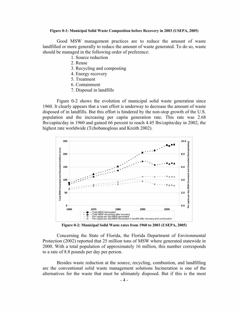
Figure 0-1: Municipal Solid Waste Composition before Recovery in 2003 (USEPA, 2005) Good MSW management practices are to reduce the amount of waste landfilled or more generally to reduce the amount of waste generated. To do so, waste should be managed in the following order of preference: 1. Source reduction 2. Reuse 3. Recycling and composting 4. Energy recovery 5. Treatment 6. Containment 7. Disposal in landfills Figure 0-2 shows the evolution of municipal solid waste generation since 1960. It clearly appears that a vast effort is underway to decrease the amount of waste disposed of in landfills. But this effort is hindered by the non-stop growth of the U.S. population and the increasing per capita generation rate. This rate was 2.68 lbs/capita/day in 1960 and gained 66 percent to reach 4.45 lbs/capita/day in 2002, the highest rate worldwide (Tchobanoglous and Kreith 2002).

0

50

100

150

200

250

1960 1970 1980 1990 2000

Tota

l MSW

Gen

erat

ed a

nd D

isca

rded

(mill

ions

tons

)

0.0

2.0

4.0

6.0

8.0

10.0

Per c

apita

per

day

MSW

Gen

erat

ed a

nd D

isca

rded

(lbs

/cap

ita/d

ay)

Total MSW GeneratedTotal MSW discarded after recoveryPer capita per day MSW generatedPer capita per day MSW discarded in landfill after recovery and combustion

Figure 0-2: Municipal Solid Waste rates from 1960 to 2003 (USEPA, 2005)

Concerning the State of Florida, the Florida Department of Environmental Protection (2002) reported that 25 million tons of MSW where generated statewide in 2000. With a total population of approximately 16 million, this number corresponds to a rate of 8.8 pounds per day per person. Besides waste reduction at the source, recycling, combustion, and landfilling are the conventional solid waste management solutions Incineration is one of the alternatives for the waste that must be ultimately disposed. But if this is the most

- 5 -

common option in Europe, it is not the case in the U.S.A. In his book American Alchemy – The History of Solid Waste Management in the United States (2003), H. Lanier Hickman Jr. gives several explanations for this, such as the opposition of environmental groups and of the public in general, the non-interest of the USEPA, the end of tax credits, and the strict air emissions regulations. Even if incineration presents important advantages (considerable reduction in waste volume, production of energy and reduction of oil dependency, production of ash used in the construction field, for instance), incineration is underdeveloped in the U.S. The preferred solution is landfilling. In 2000, about 15 percent (3.8 million tons) of MSW were incinerated, 27 percent (7.0 million tons) were recycled, and 58 percent (14.9 million tons) were disposed in landfills in the State of Florida. The goal of recycling 30 percent of the MSW flow before 1994 is not achieved, and landfills are still the most common method of final waste disposal.

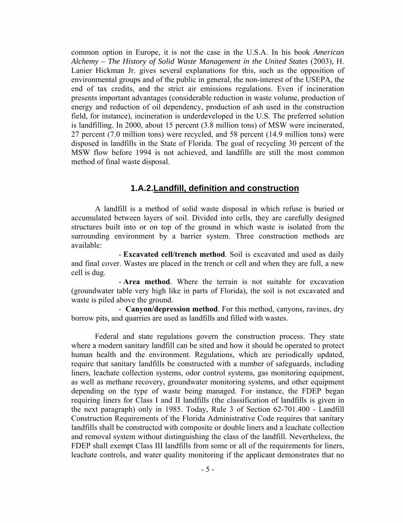
1.A.2.Landfill, definition and construction A landfill is a method of solid waste disposal in which refuse is buried or accumulated between layers of soil. Divided into cells, they are carefully designed structures built into or on top of the ground in which waste is isolated from the surrounding environment by a barrier system. Three construction methods are available: - Excavated cell/trench method. Soil is excavated and used as daily and final cover. Wastes are placed in the trench or cell and when they are full, a new cell is dug. - Area method. Where the terrain is not suitable for excavation (groundwater table very high like in parts of Florida), the soil is not excavated and waste is piled above the ground. - Canyon/depression method. For this method, canyons, ravines, dry borrow pits, and quarries are used as landfills and filled with wastes. Federal and state regulations govern the construction process. They state where a modern sanitary landfill can be sited and how it should be operated to protect human health and the environment. Regulations, which are periodically updated, require that sanitary landfills be constructed with a number of safeguards, including liners, leachate collection systems, odor control systems, gas monitoring equipment, as well as methane recovery, groundwater monitoring systems, and other equipment depending on the type of waste being managed. For instance, the FDEP began requiring liners for Class I and II landfills (the classification of landfills is given in the next paragraph) only in 1985. Today, Rule 3 of Section 62-701.400 - Landfill Construction Requirements of the Florida Administrative Code requires that sanitary landfills shall be constructed with composite or double liners and a leachate collection and removal system without distinguishing the class of the landfill. Nevertheless, the FDEP shall exempt Class III landfills from some or all of the requirements for liners, leachate controls, and water quality monitoring if the applicant demonstrates that no

- 6 -

significant threat to the environment will result from the exemption based upon the types of waste received, methods for controlling types of waste disposed of, and the results of the hydrogeological and geotechnical investigations required. Once a landfill reaches its permitted capacity, it may be expanded if permitted or it is closed and capped to prevent streaming water. It is monitored longterm to be sure that the aging process and long term performance are under control. Some research is ongoing on this subject to define the necessary timeframe of long term monitoring in years. Even after closure, contamination of soil and groundwater is still a potential issue. When no potential hazard is detectable from groundwater monitoring programs, a sanitary landfill can eventually become a new resource for the community (i.e. golf courses or recreation parks). Figure 0-3 is an illustration of the cross-section of a typical sanitary landfill.

Figure 0-3: Schematic of a Typical MSW Landfill (O'Leary and P. Walsh 1995)

The USEPA classifies landfills into two different types according to the kind of wastes they contain: - Solid Waste Landfills: These include municipal solid waste (MSW), industrial waste, construction and demolition debris, and bioreactors. Typically, MSW consist of food and garden wastes, paper products, plastics and rubber, textiles, wood, ashes (in the case of a co-disposal landfill), and the soils used as cover material. - Hazardous Waste Land Disposal Units: These include surface impoundments, waste piles, injection wells, and other geologic repositories.

- 7 -

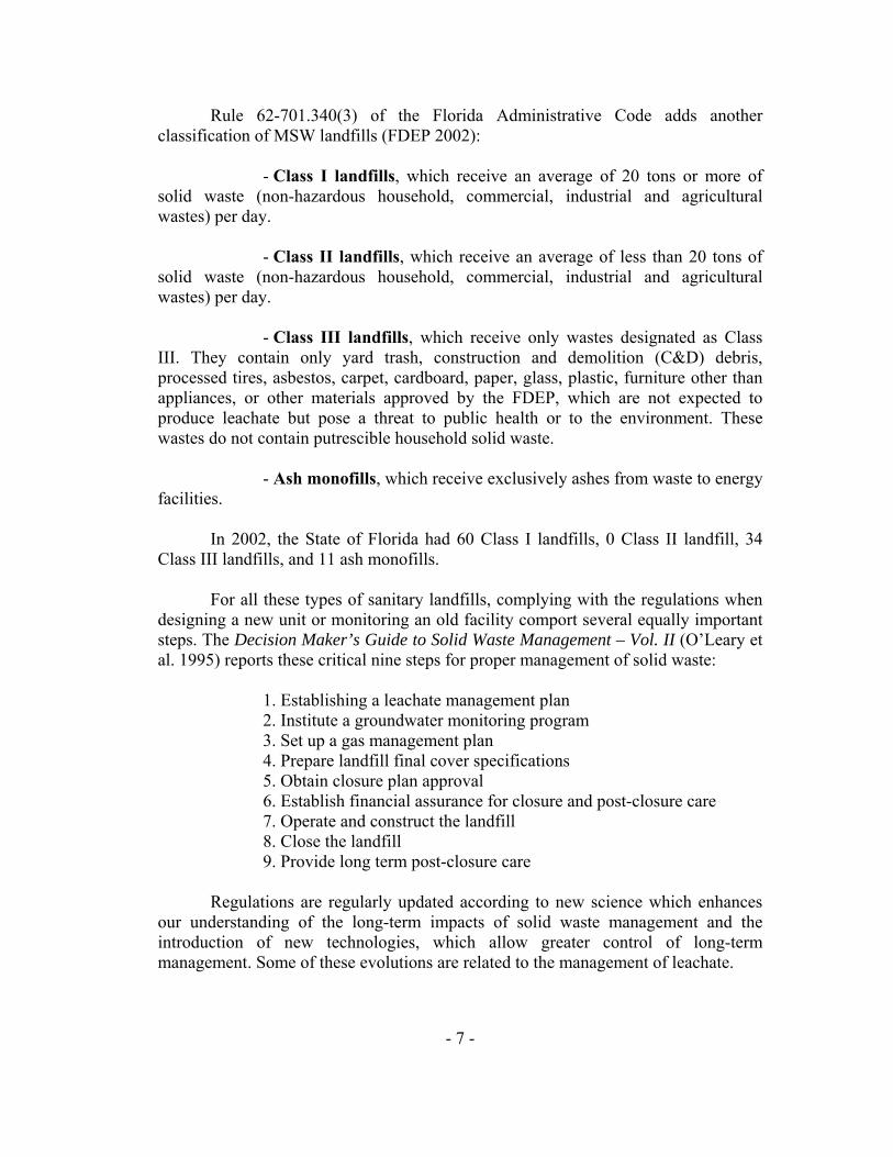
Rule 62-701.340(3) of the Florida Administrative Code adds another classification of MSW landfills (FDEP 2002): - Class I landfills, which receive an average of 20 tons or more of solid waste (non-hazardous household, commercial, industrial and agricultural wastes) per day. - Class II landfills, which receive an average of less than 20 tons of solid waste (non-hazardous household, commercial, industrial and agricultural wastes) per day. - Class III landfills, which receive only wastes designated as Class III. They contain only yard trash, construction and demolition (C&D) debris, processed tires, asbestos, carpet, cardboard, paper, glass, plastic, furniture other than appliances, or other materials approved by the FDEP, which are not expected to produce leachate but pose a threat to public health or to the environment. These wastes do not contain putrescible household solid waste. - Ash monofills, which receive exclusively ashes from waste to energy facilities. In 2002, the State of Florida had 60 Class I landfills, 0 Class II landfill, 34 Class III landfills, and 11 ash monofills. For all these types of sanitary landfills, complying with the regulations when designing a new unit or monitoring an old facility comport several equally important steps. The Decision Maker’s Guide to Solid Waste Management – Vol. II (O’Leary et al. 1995) reports these critical nine steps for proper management of solid waste: 1. Establishing a leachate management plan 2. Institute a groundwater monitoring program 3. Set up a gas management plan 4. Prepare landfill final cover specifications 5. Obtain closure plan approval 6. Establish financial assurance for closure and post-closure care 7. Operate and construct the landfill 8. Close the landfill 9. Provide long term post-closure care Regulations are regularly updated according to new science which enhances our understanding of the long-term impacts of solid waste management and the introduction of new technologies, which allow greater control of long-term management. Some of these evolutions are related to the management of leachate.

- 8 -

1.B.Leachate

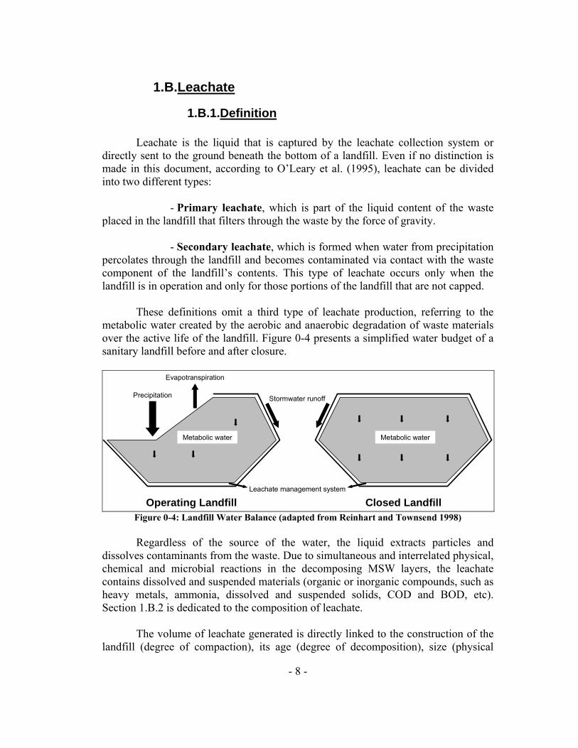
1.B.1.Definition Leachate is the liquid that is captured by the leachate collection system or directly sent to the ground beneath the bottom of a landfill. Even if no distinction is made in this document, according to O’Leary et al. (1995), leachate can be divided into two different types: - Primary leachate, which is part of the liquid content of the waste placed in the landfill that filters through the waste by the force of gravity. - Secondary leachate, which is formed when water from precipitation percolates through the landfill and becomes contaminated via contact with the waste component of the landfill’s contents. This type of leachate occurs only when the landfill is in operation and only for those portions of the landfill that are not capped. These definitions omit a third type of leachate production, referring to the metabolic water created by the aerobic and anaerobic degradation of waste materials over the active life of the landfill. Figure 0-4 presents a simplified water budget of a sanitary landfill before and after closure.

Closed LandfillOperating Landfill

Precipitation Stormwater runoff

Evapotranspiration

Metabolic water Metabolic water

Leachate management system

Figure 0-4: Landfill Water Balance (adapted from Reinhart and Townsend 1998)

Regardless of the source of the water, the liquid extracts particles and dissolves contaminants from the waste. Due to simultaneous and interrelated physical, chemical and microbial reactions in the decomposing MSW layers, the leachate contains dissolved and suspended materials (organic or inorganic compounds, such as heavy metals, ammonia, dissolved and suspended solids, COD and BOD, etc). Section 1.B.2 is dedicated to the composition of leachate.

The volume of leachate generated is directly linked to the construction of the landfill (degree of compaction), its age (degree of decomposition), size (physical

- 9 -

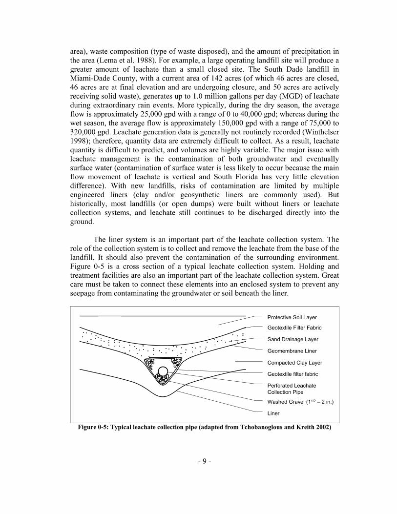
area), waste composition (type of waste disposed), and the amount of precipitation in the area (Lema et al. 1988). For example, a large operating landfill site will produce a greater amount of leachate than a small closed site. The South Dade landfill in Miami-Dade County, with a current area of 142 acres (of which 46 acres are closed, 46 acres are at final elevation and are undergoing closure, and 50 acres are actively receiving solid waste), generates up to 1.0 million gallons per day (MGD) of leachate during extraordinary rain events. More typically, during the dry season, the average flow is approximately 25,000 gpd with a range of 0 to 40,000 gpd; whereas during the wet season, the average flow is approximately 150,000 gpd with a range of 75,000 to 320,000 gpd. Leachate generation data is generally not routinely recorded (Winthelser 1998); therefore, quantity data are extremely difficult to collect. As a result, leachate quantity is difficult to predict, and volumes are highly variable. The major issue with leachate management is the contamination of both groundwater and eventually surface water (contamination of surface water is less likely to occur because the main flow movement of leachate is vertical and South Florida has very little elevation difference). With new landfills, risks of contamination are limited by multiple engineered liners (clay and/or geosynthetic liners are commonly used). But historically, most landfills (or open dumps) were built without liners or leachate collection systems, and leachate still continues to be discharged directly into the ground. The liner system is an important part of the leachate collection system. The role of the collection system is to collect and remove the leachate from the base of the landfill. It should also prevent the contamination of the surrounding environment. Figure 0-5 is a cross section of a typical leachate collection system. Holding and treatment facilities are also an important part of the leachate collection system. Great care must be taken to connect these elements into an enclosed system to prevent any seepage from contaminating the groundwater or soil beneath the liner.

Protective Soil Layer

Geotextile Filter Fabric

Sand Drainage Layer

Geomembrane Liner

Compacted Clay Layer

Geotextile filter fabric

Perforated Leachate Collection Pipe

Washed Gravel (11/2 – 2 in.)

Liner

Figure 0-5: Typical leachate collection pipe (adapted from Tchobanoglous and Kreith 2002)

- 10 -

If leachate reaches a water body, the pollution can result in rapid oxygen depletion, changes in the fauna and flora, and contamination of an aquiferor soil strata with potential migration offsite. A portion of the contaminants may remain in the soils because of their filtration and adsorption capacities. Eventually, leachate leaks can also be responsible for the generation of landfill gas outside of the perimeter of the landfill (Robinson et al. 1992). Clearly, leachate management is dependant upon the nature and concentration of specific constituents.

1.B.2.Typical composition While in operation, a landfill is constructed during several decades in a series of cells. Consequently, it contains wastes of completely different ages and different stages of decomposition. Landfill maturity can be classified into different phases. (Pohland and Harper (1986) divided the life cycle of a landfill into five successive stages: - I. Initial adjustment phase. During this phase, which takes place just after the placement of the refuse in the landfill, the aerobic biodegradation of organic compounds occurs. The daily soil cover is the main provider of the organisms responsible for this decomposition. - II. Transition phase. The air trapped inside the landfill is depleted and anaerobic conditions develop rapidly. If leachate is produced, the pH starts to diminish due to the production of organic acids and CO2 within the decomposing waste, as a result of anaerobic microbial activity. - III. Acid phase. This phase is the continuation of the previous the transition phase with high production of organic acids. As a result, the pH in leachate is rapidly reduced, H2 gas is generated, both biochemical and chemical oxygen demand (BOD and COD) increase during this phase. The low pH also helps to dissolve inorganic constituents such as metals, which increases the conductivity and total dissolved solids (TDS). - IV. Methane fermentation phase. During this phase, certain microorganisms convert the organic acids into methane (CH4) and carbon dioxide (CO2). As the organic acids are consumed, the pH starts to rise to a more neutral value, and BOD, COD, conductivity, and metals content decreases.

- V. Maturation phase. This phase begins when all the biodegradable materials have been converted into CH4 and CO2. The leachate produced is weaker in terms of contaminant concentrations, and the BOD5/COD ratio is very low.

- 11 -

The duration of the phases varies because of the construction process of the landfill. For example, a new cell can be placed on top of one which is already in the third phase. The resulting leachate will be a mixture of the characteristics of the two phases. Figure 0-6 shows the typical composition of leachate according to the different phases.

I II III IV V

Phases

Time

Leac

hate

Cha

ract

eris

tics

COD

Metals

pH

Figure 0-6: Role of phases in the leachate composition (adapted from Tchobanoglous and Kreith

2002) Several reviews have already been accomplished with the goal of collecting leachate composition according to the location (i.e. the climate and especially the precipitation rate), the age of the landfill, or the type of wastes. Different data sets are available from different parts of the world. Basically, the available leachate quality data sets lead to the same conclusion: the composition of leachate is highly variable. Differences can be as high as several orders of magnitude. Typically, the most environmentally significant parameters of leachate quality are ammonia, BOD5, COD, TDS, and heavy metals concentration: - Ammonia (NH3) is a gas at standard temperature and pressure. It is mainly used to produce fertilizer and is generated during the anaerobic digestion of organic material. As it has a high solubility in water, the gas readily transfers to leachate. - Biochemical Oxygen Demand (BOD5) is a test used to measure the concentration of biodegradable organic matter present in a sample of water. It is the amount of oxygen that would be consumed if all the organics in one liter of water were oxidized by microorganisms..

- 12 -

- Chemical Oxygen Demand (COD) is a test used to indirectly measure the amount of organic compounds (both recalcitrant and biodegradable) in water. It is the amount of oxygen that would be consumed if all the organics in one liter of water were oxidized by a strong chemical oxidant such as dichromate (Cr2O7

2-). - Total Dissolved Solids (TDS) are the total amount of charged ions, including minerals, salts, or metals dissolved in water. TDS is directly related to the purity of water and its conductivity. - Heavy metals include some of the trace metals such as cobalt, copper, manganese, vanadium, or zinc, which are required as micronutrients to sustain microbial populations, but excessive levels can be detrimental to them. Other heavy metals such as mercury, lead, or cadmium have no known vital or beneficial effect on organisms, and their accumulation over time are biotoxic and can cause serious illness in human populations. For these constituents, Table 0-1 summarizes the variability of constituents found in leachate. Conditions are not indicated in the table; it is just an indicator of the variety of leachate water quality that can be found.

Table 0-1: Extreme values for the composition of leachate (Adapted from Reinhart and Grosh (1998), Kjeldsen et al. (2002), Bernard et al. (1997), Solid Waste Authority of Palm Beach County

(2004 data), Tammemagi (1999), Tatsi et al. (2003), Oweis and Kehra (1998), Wahab et al. (2004))

ParametersLowest Value

Higest Value

Average Value

2.0 11.3 7.5

Concentration

0.4 152,000 10,300

BDL 80,800 4,000

10.0 45,000 840

0.1 8,750 830

pH

BDL* 5.0 0.1

5.2 95,000 13,100

0.0 88,000 11,000

TSS in mg/L

Ammonia in mg/L as N

COD in mg/L

BOD5 in mg/L

Lead in mg/L

Conductivity in μS/cm

TDS in mg/L

For comparison purposes, Table 0-2 shows the concentrations of the same constituents in typical medium strength untreated domestic wastewater and average concentrations of leachate.

- 13 -

Table 0-2: Comparison of the composition of untreated domestic wastewater and leachate (Adapted from Metcalf and Eddy (2003)

Wastewater Leachate

ParametersMedium strength

Average Value

7.5

Concentration

pH n/a

10,300

BOD5 in mg/L 190 4,000

COD in mg/L 430

840

Ammonia in mg/L as N 25 830

TSS in mg/L 210

13,100

TDS in mg/L 500 11,000

Conductivity in μS/cm n/a

Lead in mg/L n/a 0.1

It is clear that leachate is a highly concentrated waste stream. In general, leachates contain the same constituents at 1-2 orders of magnitude higher than medium strength domestic wastewater. The average TDS and TSS concentrations in leachate are respectively 22 and 4 times larger than medium strength wastewater, ammonia is 33 times more concentrated in leachate, and BOD5 and COD are about 24 and 21 times larger in leachate than in the medium strength wastewater.

As this research will address leachate from Florida, the literature review was particularly focused on collecting data from Florida landfills. Previous research conducted by Ward et al. (2002) and Statom et al. (2004) were also been considered. In addition, data have been collected from the Solid Waste Authority of Palm Beach County and during a record

review with Andrell Maxie at the FDEP Regional Office in West Palm Beach, FL, several reports were made available for Tammy Martin (MSCE candidate) to extract laboratory results of leachate composition from landfills in St. Lucie, Okeechobee, Broward, and Miami-Dade

counties. The complete table can be found in the Appendix A, and

Table 0-3 below contains a summary of this analysis.

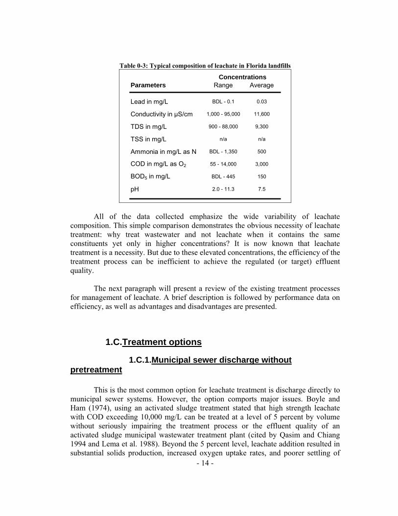
- 14 -

Table 0-3: Typical composition of leachate in Florida landfills

Parameters Range Average

BDL - 445 150

2.0 - 11.3 7.5

BDL - 1,350 500

55 - 14,000 3,000

n/a n/a

900 - 88,000 9,300

Concentrations

BDL - 0.1 0.03

1,000 - 95,000 11,600

COD in mg/L as O2

BOD5 in mg/L

TSS in mg/L

Lead in mg/L

pH


TDS in mg/L


All of the data collected emphasize the wide variability of leachate composition. This simple comparison demonstrates the obvious necessity of leachate treatment: why treat wastewater and not leachate when it contains the same constituents yet only in higher concentrations? It is now known that leachate treatment is a necessity. But due to these elevated concentrations, the efficiency of the treatment process can be inefficient to achieve the regulated (or target) effluent quality. The next paragraph will present a review of the existing treatment processes for management of leachate. A brief description is followed by performance data on efficiency, as well as advantages and disadvantages are presented.

1.C.Treatment options

1.C.1.Municipal sewer discharge without pretreatment This is the most common option for leachate treatment is discharge directly to municipal sewer systems. However, the option comports major issues. Boyle and Ham (1974), using an activated sludge treatment stated that high strength leachate with COD exceeding 10,000 mg/L can be treated at a level of 5 percent by volume without seriously impairing the treatment process or the effluent quality of an activated sludge municipal wastewater treatment plant (cited by Qasim and Chiang 1994 and Lema et al. 1988). Beyond the 5 percent level, leachate addition resulted in substantial solids production, increased oxygen uptake rates, and poorer settling of

- 15 -

biomass; leachate should be more diluted and the detention time increased. These researchers also suggested that the presence of metals, ammonia, other toxins, and extremely high organic load in leachate may cause severe upsets in the biological reactors. Cited by Qasim and Chiang (1994), Chain and DeWalle (1977) are also reported to have found that leachate greater than 5 percent by volume reduced the treatment plant efficiency. But, Raina and Mavinic (1985) have successfully treated laboratory scale combinations of 20 to 40 percent leachate by volume with municipal wastewater in aerobic batch (fill and draw) reactor with sludge residence times of 5, 10 and 20 days. Zachopoulos et al. (1990) studied co-disposal of leachate in Publicly Owned Treatment Works (POTW’s) and concluded that leachate can be treated without any adverse effect plant performance. Pohland and Harper (1985) also reported a success with combined leachate treatment in wastewater treatment plants. In their investigation BOD5 and COD removal efficiency (over 90 percent) and complete nitrification (over 80 percent) was obtained with 10-day sludge residence times. The literature reports many uncertainties about treatment efficiency and volume percentage. Although BOD5, COD and also metals reduction have been demonstrated, the results are highly variable and difficultly reproducible. A case by case study should be conducted in order to get the most cost effective and efficient treatment. Poorly clarified effluent, sludge bulking, corrosion of plant equipment and increases in effluent COD are potential operational issues.

1.C.2.Evaporation Natural pond systems are used to concentrate the constituents of the leachate, while reducing the volume through evaporation. The process occurs in impervious lined basins with no discharge and is highly dependent on climate conditions. Temperature, precipitation, wind and humidity will affect the rate of evaporation. This process may be a solution to separate the water from the contaminants but it presents several inconveniences. First, the residues have to be treated afterwards and secondly, natural evaporation ponds can not be easily applied in Florida due to the tropical weather. Ultimately, the leachate pollutants are in higher concentration (Di Palma et al. 2002) or in a solid form but they are not treated: post treatment is required. Evaporation can also be executed in a reactor, but similar problems would be encountered. Nevertheless, in their laboratory testing, these researchers achieve produce a distillate containing 99 percent less COD, 85 percent less ammonia and removed all the lead. In return, the concentrations of the same constituents are much higher in the residue.

1.C.3.Deep well injection Underground Injection Control (UIC) is a very inexpensive way (Saripalli et al. 2000) to dispose of a waste stream without treatment and without further surface and human contact. No treatment is generally performed on the leachate and the

- 16 -

pollution problem is not addressed. Constituents of leachate are transferred to the host formation and the groundwater. This may become an issue if this groundwater reaches an aquifer used as a drinking water source. Surface water is equally at risk in the case of a spill during the transport of the waste. Also, the same authors demonstrated that the well performances are subject to a rapid decline if the TSS content of the injected liquid is high. This is very often the case for leachate. In a near future, this option may not be acceptable anymore as the regulations become more and more stringent. The number of active deep wells already started to diminish: 819 deep well injection installations (including industrial, municipal and nuclear sectors) were counted in 1986 in the US, but only 485 were still in operation in 1991.

1.C.4.Hauling off-site Off-site hauling does not directly address the pollution problem either. The leachate is just moved to another location. The option presents a high transportation risk and is an expensive solution. In Polk County (FL) the cost is $110 per 1,000 gallons for transportation and pre-treatment prior to discharge into the wastewater system. (Note: after a phone conversation with the Solid Waste Division of Polk County, it appears that a bioreactor is currently experimented under the supervision of T. G. Townsend of the University of Florida, in order to reduce the amount of hauled leachate.)

1.C.5.Leachate recirculation: bioreactor This innovative option consists of the re-injection of the collected leachate back into the landfill so that it percolates again through the waste. The goal is to transform the landfill into an aerobic reactor. By recycling the leachate, the organic load may be reduced by the microorganisms present in the waste. Morris et al. (2003) reported that with the exception of ammonia, it was found that the concentrations of the BOD, heavy metals, chlorinated VOCs, and benzene, toluene, ethylbenzene, and total xylenes (BTEX) were reduced to below drinking water standards after 5 years of closure and following 7 years of leachate recirculation in a MSW landfill facility (located at the Central Solid Waste Management Center in Sandtown, Delaware). Conductivity was reduced from 12,000 to 8,400 μSm/cm2, ammonia was reduced from 600 to 400 mg/L as N, and BOD was reduced by 99 percent with an initial value of 40,000 mg/L. Pohland (1972, 1975, 1980) and Pohland et al. (1990) found that when leachate was continuously collected and reapplied to an experimental landfill column, the organic loading of the leachate decreased to a small fraction of its peak value (i.e. from 20,000 mg/L of COD to less than 1,000 mg/L) in a period of just over a year (cited by Qasim and Chiang 1994). This reduction in the leachate quality and quantity has the advantage of lowering the cost of post-treatment. Leachate recirculation also presents the advantages of enhancing the gas generation and improving the rate of landfill stabilization by enhancing the biodegradation of the

- 17 -

refuse; thereby; increasing the landfill life time and reducing the operating costs. Recycling leachate is one of the least expensive options (Lema et al. 1988). However, these advantages cannot hide the fact that recirculation system represents a substantial investment, and depending on the local requirements post-treatment of leachate may still be necessary if the recirculated leachate does not reach the allowable discharges limits (Lema et al. 1988, Winthelser 1998).

1.C.6.On-site treatment On-site systems used to attenuate constituent’s concentrations in leachate can be designed using many different unit processes. They are deployed as pretreatment prior to discharging the effluent to a wastewater treatment facility, or to the environment if it meets the permit requirements. On-site treatment systems can be separated into two categories: biological and physicochemical processes.

1.C.6.a.Biological processes Biological processes are based on the action of a mixed culture of microorganisms in an aerobic or anaerobic environment. Treatment can be accomplished via activated sludge systems, waste equalization ponds, aerated lagoons, trickling filters, rotating biological contactors, or anaerobic digesters. These methods are equivalent to discharging to an off-site wastewater treatment plant and as a result have the same disadvantages, namely: 1) they do not address bio-toxic constituents, and 2) their efficiency is highly dependent on the effluent composition and strength. Now, landfill leachate has been demonstrated to have volumes and concentrations that are highly variable. Therefore, these processes may have a limited impact of leachate quality and should be considered as a first step of a more comprehensive process (for instance: the pretreatment of leachate prior to discharge into the sewer system). Aerobic processes transform the organic matters in CO2 and organic sludge; anaerobic treatment processes mainly transform the organic matters in CO2, CH4 and a minor part in sludge (Lema et al. 1988). The sludge production may be an issue as aerobic treatment produces appreciable amounts of biomass residuals resulting in a subsequent problem of disposal (residual presence of heavy metals) as well as odor generation. Using acclimated sludge, Anagiotou et al. (1993) removed 93, 45, and 97 percent of COD, BOD5, and ammonia in 14 days. Initial concentrations were 920 mg/L, 6,765 mg/L, and 3,300 mg/L. The percentage removal may be significant concerning ammonia and BOD5, but not for COD. Also, the residence time of half a month has to be underlined. In practice, this would require large amounts of available space, which is extremely valuable at a sanitary landfill site. Thus a large footprint would represent an effective loss of capacity for the landfill area of the facility. For example, if this technique was applied at the South Dade Landfill in Miami-Dade

- 18 -

County, the aeration basins would have a volume of 280,00 ft3 if the design is made with the average flow during the wet season. Only for the aeration basins, this represents an area of 14,300 ft2 (0.33 acre) at a depth of 20 ft. Lema et al. (1988) reported different researches using a variety of detention time, temperature or nutrients ratio. Processes are not always efficient, but more importantly, the major issue reported here is that the efficiency is difficultly reproducible. Leachate quality and quantity are too variable to maintain a constant effluent quality and specific treatment conditions are necessary for each type of leachate (young or old, highly diluted or no). Similar conclusions can equally be drawn concerning the anaerobic processes.

1.C.6.b.Physical and chemical processes Physical and chemical processes utilize the addition of chemical or mechanical means to ensure treatment. They are often used with in conjunction with a biological process (Lema et al 1988). The common chemical processes are: - Coagulation, flocculation, chemical precipitation and sedimentation. They are fully developed processes used in the removal of precipitable substances, such as soluble heavy metals, dissolved organics and colloidal particles suspended in the liquid. While they are independent mechanisms, they are interrelated and often used in conjunction of one anther. More details will be given with the physical processes of flocculation and sedimentation. - Carbon adsorption. Activated carbon is used in water treatment due to its high adsorptive surface area. Reported studies showed COD and BOD5 removal of respectively 91 and 65 percent using biologically pretreated leachate (Morawe et al. 1995). But initial BOD5 was very low: approximately 3 mg/L and initial COD was in the order of 900 mg/L. Using activated carbon grains, Abdel-Halim et al. (2003) reached an uptake of 89 percent on lead contained in industrial or synthetic wastewater. The initial lead concentration was 4 mg/L. This value is on the high range of the concentrations found in leachate. In a second experiment, the initial concentration was 10 mg/L and the removal efficiency dropped of less than 3 points to 86.4 percent. Other researches by Copa and Meidl (1986) demonstrated the benefits of combining an aerobic treatment with the granulated activated carbon technology. With 12 days of detention time, they achieved a complete removal of BOD5 (initial concentration of 30 mg/L). 77, 98 and 46 percent of respectively COD (initial concentration of 920 mg/L), ammonia nitrogen (initial concentration of 210 mg/L) and SS (initial concentration of 210 mg/L) were degraded. In a second step, they implemented their treatment process with sand filters and a second stage of granular activated carbon treatment and increased the removal of COD and SS to 90 and 99 percent. The activated carbon technology is especially an efficient technique in removing non-biodegradable compounds. But this is considered to be an expensive

- 19 -

solution due to the necessity of frequent media regeneration in column reactor or high quantity of carbon powder (Lema et al. 1988). In leachate treatment, this is also typically the case as carbon has to be regenerated more often due to the high concentrations of impurities. - Ion exchange. Ion exchange involves the interchange of ions between an aqueous solution and a solid material: the ion exchanger. The main use of this process is water softening to reduce concentrations of magnesium and calcium using sodium ions. In wastewater treatment, it is used for the removal of nitrogen, heavy metals or TDS. Zeolites are natural ion exchange materials; synthetic materials are aluminosilicates, resins or phenolic polymers. Street et al. (2002) reported that a novel polyacrylate-based ion-exchange material will remove modest amounts of Pb (high-ppm concentration range) and reduce the Pb concentration to the low-parts per billion range. Likewise, Papadopoulos et al. (1996) used clinoptilolite (microporous mineral form the group of zeolites) in a sodium form in an ion exchange reactor. A maximum removal of 83 percent of ammonia was achieved with a starting concentration of 2,700 mg/L. They also achieved 15 percent removal of BOD5, with a starting concentration of 8,500 mg/L. Unfortunately, the ion exchange technology requires highly costly resin regeneration or replacement (Escobar et al. 2006). Also, to be efficient, this process requires preliminary treatment. Those are the two main explanations why this technology is not more spread in water operations. The common physical processes are: - Air stripping. This technology is used to remove ammonia and volatile organic compounds (VOCs). The mechanism involved in air stripping is the transfer of a gas from the liquid phase to the gas phase. This is accomplished by contacting the liquid containing the gas with a gas (usually air) that does not contain the gas initially. However, air stripping does not address the other components of the leachate flow, such as BOD5, COD or metals. Consequently, it cannot be used on its own. Also, air stripping of ammonia requires a pH adjustment to a value near 11 which is usually done using lime (Lema et al. 1988). For instance, after 96 hours, Silva et al. (2003) achieved a removal of 99.4 percent of ammonia with an initial concentration of 880 mg/L as N. It should be noted that during the same experiments, ammonia was not removed by coagulation/flocculation or membrane fractionation. - Flocculation and sedimentation. Coagulation, precipitation, flocculation, and sedimentation are fully-developed and have long been used in water treatment. They are generally practical, effective and relatively low-cost for water softening, phosphorus and heavy metal removal, removal of turbidity and suspended particles. Common coagulants are lime, alumina, FeCL3 or FeSO4. Silva et al. (2003) reported 25 percent removal of COD, but no removal of ammonia using coagulation with aluminum sulfate and flocculation. Wu et al. (2004) reported a removal of 60 percent of COD using ferric chloride as coagulant. Amokrane et al. (1997) used coagulation with ferric chloride, flocculation and sedimentation to achieve 54 percent

- 20 -

removal of COD. These processes are generally very efficient to remove color, TSS, ammonium, heavy cations; but show limited removal of COD. The literature reported here on these processes shown that they are mostly used prior to additional treatment such as ozonation or advanced oxidation processes. - Filtration. Filtration is a solid/liquid separation technique. It is also generally employed before advanced treatment processes. Microfiltration, ultrafiltration, nanofiltration and reverse osmosis (RO) are variations of membrane filtration process. In that order, they produce an effluent with a higher and higher quality, but the brine, which contains concentrated constituents, must be handled separately. They usually constitute the last stage of a process that may consist of biological treatment. Slater et al. (1983) reported after initial treatment (oil separation, coagulation by lime, recarbonation, and pH adjustment) 98, 68, and 59 percent removal of TDS, COD, and TOC using a RO unit with a permeate flux of 4.4 gpd/ft2 (initial concentrations were respectively 16,400, 26,400 and 8,500 mg/L) (cited by Qasim and Chiang 1994). Removals of up to 90 percent of NH3-N, 91 percent of BOD5, 98 percent of COD, and 99 percent of the electrical conductivity have been reported also using a RO system (Ushikoshi et al. 2002). Other research (Linde et al. 1995) showed similar removal efficiencies. However, disposal of filtration processes concentrates is a serious problem (Peters 1998). High salt concentration in the leachate may as well cause membrane fouling and low membrane flux. And if ultrafiltration and RO can generate high quality filtrates, they are also known to be expensive processes (Escobar et al. 2006). Physical and chemical processes present the advantages of being immediately functional, simples, insensitive to temperature variations. However, they generally generate great quantities of sludge and the costs of chemical and materials are high (Lema et al. 1988). Reviewing all of these available methods to treat landfill leachate leads to the eventual conclusion that none of them is efficient from a long-term perspective. Each has advantages and limitations, but none can achieve consistent removal of the major constituents of concern while generating environmentally-friendly effluent and residuals. Formulating a global recommendation for leachate treatment is not possible. A combination of several methods can be used, but the cost will then become prohibitive: effluent and residuals quality is high if treatment is expensive and conversely. Consequently, an all inclusive solution is currently not available for long-term leachate management. Thus, new technologies must be considered and further studies made. One of the potential solutions may involve advanced oxidation processes (AOPs) or energized processes (EPs).

1.C.7.Alternative treatment methods: AOPs and EPs

- 21 -

Chemical oxidation is an on-site chemical treatment used for the destruction of organics and precipitation of metals. It is based on oxidation-reduction reactions. Advanced oxidation processes were defined by Glaze et al. in 1987 as "near ambient temperature and pressure water treatment processes, which involve the generation of hydroxyl radicals in sufficient quantity to effect water purification.'' An AOP uses ozone (O3), hydrogen peroxide (H2O2) or other agents to oxidize the pollutants through the production of the hydroxyl radical (OH•). OH• is a powerful and indiscriminate oxidant (relative oxidation power of 2.05 compared to 1.00 for chlorine, Table 0-4 presents the relative oxidation power of the species used in AOPs), which oxidizes pollutants into components that are less harmful for the environment. Hydroxyl radicals are capable of achieving complete mineralization (i.e. degrading to CO2, H2O and mineral ions) virtually all organic compounds (Feitz et al. 1998). Those that are only partially oxidized are degraded into more biodegradable or more easily separable by-products (Schulte et al. 1995). An energized process (EP) is based on the same mechanisms with the additional action of ultraviolet (UV) light, which may be either from a UV lamp or from natural sunlight. Addition of ultraviolet energy has been shown to enhance the production of the hydroxyl radical. Steensen (1997) explained that without activation by iron salt or UV radiations, the oxidation power of the oxidants is far less than with this activation. The use of iron or photo-energy improves this oxidation power by forming hydroxyl radicals. He also reported the work of Staehelin and Hoigné (1983) about "radical scavengers": carbonates species (CO3

2- / HCO3-) or alkyl compounds slow down the reaction rate because they

can interrupt the chain reaction. Maintaining a low pH is important for this type of processes. Nevertheless, AOPs and EPs offer a robust and increasingly economically favorable alternative for treatment of wastewaters contaminated with highly toxic organic constituents (Feitz et al. 1998). They are known to handle many of the constituents typically found in leachate: - Elevated ammonia: EPs convert ammonia to nitrate through aeration and promote stripping of NH3(g). - High COD/BOD ratios: EPs convert refractory COD into readily biodegradable BOD (Suty et al. 2004). - Heavy metals (Pb, As, Cd, Hg): EPs remove heavy metals through co-precipitation, adsorption, and redox mechanisms. - pH toxicity: EPs minimize pH impacts as a byproduct of aeration treatment. - VOCs: EPs can destroy recalcitrant organics and promote stripping of VOC’s during aeration (Suty et al. 2004).

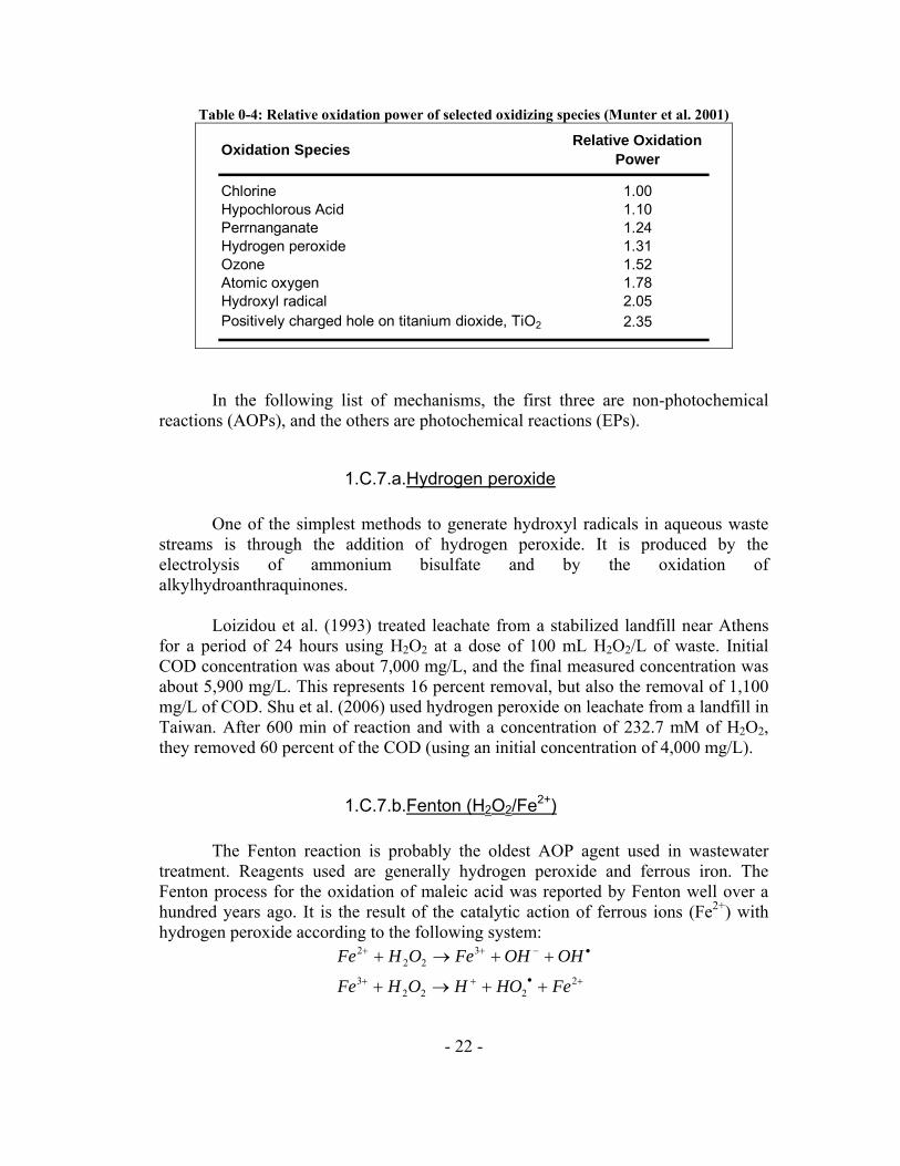
- 22 -

Table 0-4: Relative oxidation power of selected oxidizing species (Munter et al. 2001)

Oxidation Species Relative Oxidation Power

Chlorine 1.00Hypochlorous Acid 1.10Perrnanganate 1.24Hydrogen peroxide 1.31Ozone 1.52Atomic oxygen 1.78Hydroxyl radical 2.05Positively charged hole on titanium dioxide, TiO2 2.35

In the following list of mechanisms, the first three are non-photochemical reactions (AOPs), and the others are photochemical reactions (EPs).

1.C.7.a.Hydrogen peroxide One of the simplest methods to generate hydroxyl radicals in aqueous waste streams is through the addition of hydrogen peroxide. It is produced by the electrolysis of ammonium bisulfate and by the oxidation of alkylhydroanthraquinones. Loizidou et al. (1993) treated leachate from a stabilized landfill near Athens for a period of 24 hours using H2O2 at a dose of 100 mL H2O2/L of waste. Initial COD concentration was about 7,000 mg/L, and the final measured concentration was about 5,900 mg/L. This represents 16 percent removal, but also the removal of 1,100 mg/L of COD. Shu et al. (2006) used hydrogen peroxide on leachate from a landfill in Taiwan. After 600 min of reaction and with a concentration of 232.7 mM of H2O2, they removed 60 percent of the COD (using an initial concentration of 4,000 mg/L).

1.C.7.b.Fenton (H2O2/Fe2+) The Fenton reaction is probably the oldest AOP agent used in wastewater treatment. Reagents used are generally hydrogen peroxide and ferrous iron. The Fenton process for the oxidation of maleic acid was reported by Fenton well over a hundred years ago. It is the result of the catalytic action of ferrous ions (Fe2+) with hydrogen peroxide according to the following system:

+•++

•−++

++→+

++→+2

2223

322

2

FeHOHOHFe

OHOHFeOHFe

- 23 -

The reaction is eased by low pH, often resulting in pH adjustment. Because of the use of iron, sludge can be generated in high quantity. An additional step such as sedimentation is generally required after the Fenton process. Loizidou et al. (1993) also treated leachate from a stabilized landfill near Athens, Greece, for a period of 24 hours using 40 mg/L of FeSO4 and 100 mL H2O2/L of waste. The initial COD concentration was about 7,000 mg/L, and the final measured concentration was about 4,550 mg/L. This represents 35 percent of removal. For BOD5, the removal was 18 percent (initial concentration around 3,400 mg/L and final concentration 2,800 mg/L). Lopez et al. (2004) also treated raw leachate with the Fenton process. After adjusting the pH to 3.0, adding 10,000 mg/L of H2O2, and 830 mg/L of Fe2+, they demonstrated a maximum removal of 60 percent with a detention time of 2 hours. Initial COD concentration was 10,540 mg/L. Englehardt et al. (2005) used the Fenton process on pre-filtered and pH-adjusted leachate and achieved 61 percent removal of COD and 14 percent removal of ammonia.

1.C.7.c.Ozone Glaze et al. (1987) stated that ozone has been used as a chemical reagent, an industrial chemical, and an oxidant for water treatment for over eight decades. Ozone is known to be a powerful oxidant and disinfectant, with a thermodynamic oxidation potential that is the highest of the common oxidants. In principle, ozone should be able to oxidize inorganic substances to their highest stable oxidation states and organic compounds to carbon dioxide and water to achieve complete mineralization. In practice however, ozone is known to be selective in its oxidation reactions. In water treatment, ozone has been most successful for enhancing the pleasant taste of water, for aiding coagulation and filtration processes, and as a first barrier to microorganisms. Imai et al. (1998) reported 35 percent removal of COD by using ozone with a contact time of 10 min. Then, they used the effluent of this treatment in two biological activated carbon fluidized bed reactors in series (anaerobic and aerobic with a 24 hours detention time) and improved the treatment to 63.5 percent removal of COD. At the same time, they also achieved 75 percent removal of BOD5.

1.C.7.d.Ozone and hydrogen peroxide The addition of hydrogen peroxide to ozone offers an alternative way of generating the hydroxyl radical. The global reaction mechanism is the following:

2223 322 OOHOHO +→+ •

- 24 -

The use of ozone and hydrogen peroxide has the double effect of generating hydroxyl radical and directly oxidizing the contaminants by their proper oxidizing action. This combination is notably employ for water which is relatively impermeable to UV and for large flow volumes (Schulte et al 1995).

1.C.7.e.Ultraviolet light Ultraviolet light is known to enhanced the production of the hydroxyl radical (Schulte et al 1995), but this is not is only action in water treatment. Indeed, the same authors explained that “because of their property of absorbing UV-light, many molecules are destroyed directly by UV-light or are activated by it, thus making them more easily oxidizable”.

1.C.7.f.Photo-Fenton / Fenton-like systems A photo-Fenton process consists of the addition of ferric iron (Fe3+) to a H2O2/UV system. At low pH, the Fe(OH)2+ complex is formed and is subsequently oxidized by UV radiation according to the following reaction sequence:

( )•++

++

+⎯→⎯

+→++

OHFeOHFe

HOHFeOHFehv 22

22

3

)(

Soo-M. Kim et al. (1997) used this process on municipal landfill leachate. Leachate was pre-treated biologically and pH was adjusted to 3.0. The optimum conditions obtained for the best degradation were: a concentration Fe(II) on the order of 1.0 x 10-3 mol.L-1 (56 mg/L) and a molar ratio COD/H2O2 = 1/1. The UV energy was set to 80 kW.m-3. The starting COD concentration was 1,150 mg/L and after two hours of treatment, the removal obtained was 70 percent.

1.C.7.g.Ultraviolet light and hydrogen peroxide The direct photolysis of hydrogen peroxide leads to the formation of OH• radicals by the hemolytic splitting of the oxygen-oxygen bond (Schulte et al 1995):

•⎯→⎯ OHOH hv 222

Shu et al. (2006) enhanced the efficiency of their first experiment with H2O2 (described in paragraph 1.C.7.a) only by adding four UV lamps. With this new set-up, they improved the COD removal of 5 points (from 60 percent with hydrogen peroxide only) and reduced the reaction time by 50 percent (600 min to 300 min). The formation of OH• was greatly improved by the addition of UV energy.

- 25 -

1.C.7.h.Ultraviolet light and ozone Ozone readily absorbs UV radiation to form H2O2, which will decompose into hydroxyl radicals by the following mechanism:

•+→++ OHOhvOHO 2223

Prengle and coworkers at the Houston Research Inc. (HRI) were the first to see the commercial potential of the O3/UV system (cited from Glaze et al. 1987). They showed that O3/UV enhances the oxidation of COD and BOD and also complexed cyanides, chlorinated solvents, and pesticides.

1.C.7.i.Ultraviolet light, ozone and hydrogen peroxide The addition of H2O2 to the O3/UV process accelerates decomposition of ozone, resulting in an increased rate of OH• radical production. The conjugate base of H2O2, HO2

- has been shown to initiate the mechanism (Munter et al. 2001)

−− +→+ 3232 OHOOHO

This step initiates the decomposition of ozone resulting in the production of the hydroxyl radical. Ince (1998) achieved 89 percent removal of COD with an initial concentration of 1,290 mg/L, while using these three oxidants (UV, O3, and H2O2). In the absence of O3, the system could remove 59 percent of the COD. And in the absence of H2O2, the system could remove only 54 percent of the COD. The combination however enhanced the performance of the system to the 89 percent removal. But compared to the experiments conducted by Loizidou et al. (1993), using only H2O2, the actual quantities of COD removed were very similar.

1.C.7.j.Photocatalytic oxidation The photocatalysis principle resides in the excitation of a metal semiconductor by photons to produce an electron-hole pair. This pair has a very powerful oxidation potential and should be able to oxidize almost any chemical. Munter et al. (2001) proposed the following possible reaction mechanism, where “h+” is a hole, “e-” an electron, and “R” is an organic compound:

- 26 -

+•+

••

••

•−+

−•−

→+

+→+

→+

→+

→+

RHRHh

OHRRHOHRHOHRHOH

OHOHh

OOe

2

22

According to Munter et al. (2001), the presence of dissolved oxygen is necessary for this reaction to take place. It prevents the recombination of the electron-hole pair while producing H2O2:

222

22

22

OHeHHO

HOHO

OeO

⎯→←++

⎯→←+

⎯→←+

−+•

•+−•

−•−

Titanium dioxide (TiO2) is one of the most widely used metal oxides in the industry for photocatalytic applications.

1.C.7.k.Iron-Mediated Aeration (IMA) IMA has been studied on leachate during the FCSHWM-funded project entitled, “Investigation of options for management of leachate and wastewater,” directed by Dr. Englehardt (University of Miami) and Dr. Meeroff (Florida Atlantic University) (2005). They were the first to successfully demonstrate the IMA process for in-situ remediation of organic and metallic contaminants in soil and groundwater at former nuclear weapons facilities managed by the U.S. Department of Energy, in laboratory tests (2002). Then, they used the process to oxidize organics and co-precipitate inorganics in wastewater. They achieved 99.996 percent removal of arsenic and 99 percent removal of ethylenediamine tetraacetic acid (EDTA). Its reaction mechanism is not completely known, but evidence suggests that it involves: - The oxidation of Fe(s) to Fe2+ - The creation of hydroxyl radical according to the Fenton reaction - The oxidation action of hydroxyl radical - The co-precipitation action of ferric precipitates. Using the IMA process at neutral pH, Englehardt et al. (2005) reduced the COD of leachate by 56 percent, and increased the BOD5/COD mass ratio from 0.1 to 0.28. As well, the treatment achieved 83 percent reduction in ammonia and 40 percent reduction in the effluent electrical conductivity of leachate. Meeroff et al. (2006) demonstrated a preliminary cost projection below $0.05 per gallon. In addition, two logs of removal of EDTA, Cd2+, Hg2+, and Pb2+, and an average 63 percent removal

- 27 -

of Ni2+ were achieved by Englehardt et al. (2002). Cited by Englehardt et al. (2005), 1-2 logs of removal of 1.0 mg/L 17-β-estradiol (estrogen) and di-n-butyl phthalate were achieved in simulated natural water at pH 7.5 by Englehardt et al. (2003).

1.C.7.l.Photochemical Iron-Mediated Aeration (PIMA) Preliminary studies on the IMA with UV (PIMA) process have been conducted by Englehardt et al. (2005). They showed no significant difference between the PIMA and IMA technique. This result has been attributed to the reactor design of the UV source and the steel wool packing density. Meeroff et al. (2006) showed a cadmium removal of 29 percent in a PIMA reactor compared to just 5 percent in the non-energized control IMA reactor (reaction time was 256 min and initial concentration was 0.1 mol/L).

1.C.8.Ranking of treatment options

1.D.Problem statement The main conclusion drawn from this introduction is that longterm management of leachate continues to be an issue. This is due to the absence of leachate collection in many older landfills, which are continuously releasing contaminants directly into the environment. A second explanation resides in the available treatment techniques, which are not completely satisfactory. There is currently no technology that addresses all the constituents of leachate and produces a safely dischargeable effluent, without generating dangerous residuals. Some processes can lower the concentration of several constituents, but they either do not treat some others (such as air stripping or aerobic treatment) or produce an even more polluted residual (such as aerated lagoons or membrane filtration). To remedy this matter, advanced oxidation (AOPs) and energized processes (EPs) show encouraging capabilities for dealing with high strength waste waters. Among them, the new IMA technology seems capable of producing a safe dischargeable effluent, at a limited cost. Several studies cited demonstrate the active benefits of implementing a process with UV radiation. Consequently, IMA results are anticipated to be improved in terms of reaction time and removal efficiency by the utilization of UV light. The development of engineering performance data for the PIMA process for treatment of leachate is the subject of this thesis.

- 28 -

1.E.Objectives The primary objective of this thesis is to develop a laboratory scale reactor for the Photochemical Iron-Mediated Aeration process. This design was based on the development made by Meeroff et al. (2006), and a schematic of the process is shown in Figure 0-7 below.

Figure 0-7: PIMA principle

The PIMA process is an on-site treatment option. It was initially designed to be inserted into a municipal landfill leachate collection and treatment system. Nevertheless, during this experimental approach, the laboratory-scale reactor was designed to allow the researchers to conduct multiple experiments simultaneously (absence or presence of iron, for instance). The second objective is to evaluate the treatment efficiency of the PIMA process. Research, literature review, and laboratory experimentation were performed, and performance data were generated. Preliminary results of the literature review showed that the most environmentally-relevant components of typical leachate are: ammonia, BOD5, COD, dissolved solids, conductivity, and certain heavy metals. The targeted goal was to achieve the allowable concentrations for municipal sewer discharge to consider the effluent as a typical wastewater that will not disrupt the

- 29 -

operation of a typical domestic wastewater treatment plant. As the experiments were made in the Civil Engineering Department at the Florida Atlantic University in Boca Raton, FL, the allowable discharge concentrations selected were for the City of Boca Raton Sewer Use Policy Limits Regulated Pollutants. Those limits are presented in Table 0-5.

Table 0-5: Allowable sewer discharge concentrations for the City of Boca Raton, FL (Environmental Health and Safety, Florida Atlantic University, (2004). “Chemical Hygiene

Plan”, http://www.fau.edu/ (February 24, 2006)

Parameters

Maximum allowable value over any 24-hr

period

Lead in mg/L

TDS in mg/L


0.37

2,000

n/a

TSS in mg/L 400

800

21


Iron in mg/L

n/a

COD in mg/L

BOD5 in mg/L

pH

400

6.0 - 8.5

Note: For Conductivity and ammonia no limit value is listed.

The final step was to compare the experimental results with the other alternative leachate treatment options and to draw up a comparative statement regarding the removal efficiency, the anticipated cost per gallon of treated leachate, and the environmental risks associated with longterm leachate management.

- 30 -

CHAPTER 2: METHODOLOGY

- 31 -

2.A. Reactor design and construction As expressed before, the reactor was designed according to the development made by Meeroff et al. (2006). It was constructed by Eli Brossell, Courtney Skinner and Francois Gasnier and is comprised of: - A photochemical safety cabinet from Ace Glass Incorporated (Vineland, NJ) to shield the investigators from the UV radiation. A hole has been drilled in the top face of the cabinet to verify that the lamp is working properly by indirect visual inspection of the blue haze generated by the 450-W medium pressure mercury vapor lamp. - A rack which can contains spaces for 32 test tubes and a UV lamp in its center. The test tubes can be configured at three different distances from the lamp: 6.3 cm, 10.2 cm and 15.2 cm (distance from the center of the lamp to the center of the test tubes). The rack is composed of two stages. The bottom one receives the round end of the test tubes and the top one maintains them in the vertical position. The stages are linked by four shanks. Figure 2-1 is a view from above of this arrangement.

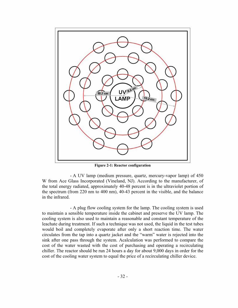
- 32 -

Figure 2-1: Reactor configuration

- A UV lamp (medium pressure, quartz, mercury-vapor lamp) of 450 W from Ace Glass Incorporated (Vineland, NJ). According to the manufacturer, of the total energy radiated, approximately 40-48 percent is in the ultraviolet portion of the spectrum (from 220 nm to 400 nm), 40-43 percent in the visible, and the balance in the infrared. - A plug flow cooling system for the lamp. The cooling system is used to maintain a sensible temperature inside the cabinet and preserve the UV lamp. The cooling system is also used to maintain a reasonable and constant temperature of the leachate during treatment. If such a technique was not used, the liquid in the test tubes would boil and completely evaporate after only a short reaction time. The water circulates from the tap into a quartz jacket and the “warm” water is rejected into the sink after one pass through the system. Acalculation was performed to compare the cost of the water wasted with the cost of purchasing and operating a recirculating chiller. The reactor should be run 24 hours a day for about 9,000 days in order for the cost of the cooling water system to equal the price of a recirculating chiller device.

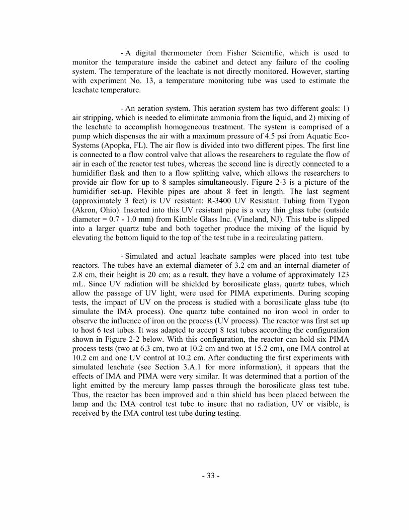
- 33 -

- A digital thermometer from Fisher Scientific, which is used to monitor the temperature inside the cabinet and detect any failure of the cooling system. The temperature of the leachate is not directly monitored. However, starting with experiment No. 13, a temperature monitoring tube was used to estimate the leachate temperature. - An aeration system. This aeration system has two different goals: 1) air stripping, which is needed to eliminate ammonia from the liquid, and 2) mixing of the leachate to accomplish homogeneous treatment. The system is comprised of a pump which dispenses the air with a maximum pressure of 4.5 psi from Aquatic Eco-Systems (Apopka, FL). The air flow is divided into two different pipes. The first line is connected to a flow control valve that allows the researchers to regulate the flow of air in each of the reactor test tubes, whereas the second line is directly connected to a humidifier flask and then to a flow splitting valve, which allows the researchers to provide air flow for up to 8 samples simultaneously. Figure 2-3 is a picture of the humidifier set-up. Flexible pipes are about 8 feet in length. The last segment (approximately 3 feet) is UV resistant: R-3400 UV Resistant Tubing from Tygon (Akron, Ohio). Inserted into this UV resistant pipe is a very thin glass tube (outside diameter = 0.7 - 1.0 mm) from Kimble Glass Inc. (Vineland, NJ). This tube is slipped into a larger quartz tube and both together produce the mixing of the liquid by elevating the bottom liquid to the top of the test tube in a recirculating pattern. - Simulated and actual leachate samples were placed into test tube reactors. The tubes have an external diameter of 3.2 cm and an internal diameter of 2.8 cm, their height is 20 cm; as a result, they have a volume of approximately 123 mL. Since UV radiation will be shielded by borosilicate glass, quartz tubes, which allow the passage of UV light, were used for PIMA experiments. During scoping tests, the impact of UV on the process is studied with a borosilicate glass tube (to simulate the IMA process). One quartz tube contained no iron wool in order to observe the influence of iron on the process (UV process). The reactor was first set up to host 6 test tubes. It was adapted to accept 8 test tubes according the configuration shown in Figure 2-2 below. With this configuration, the reactor can hold six PIMA process tests (two at 6.3 cm, two at 10.2 cm and two at 15.2 cm), one IMA control at 10.2 cm and one UV control at 10.2 cm. After conducting the first experiments with simulated leachate (see Section 3.A.1 for more information), it appears that the effects of IMA and PIMA were very similar. It was determined that a portion of the light emitted by the mercury lamp passes through the borosilicate glass test tube. Thus, the reactor has been improved and a thin shield has been placed between the lamp and the IMA control test tube to insure that no radiation, UV or visible, is received by the IMA control test tube during testing.

- 34 -

Figure 2-2: Reactor configuration with test tubes placement.

- The iron used comes from Soap Free Steel Wool Balls from Brillo. More details are provided later. The three pictures below are some illustrations of the reactor set-up.

- 35 -

Figure 2-3: Aeration and humidifier systems

Figure 2-4: View of the inside of the safety cabinet and aeration piping

- 36 -

Figure 2-5: Reactor set up prior to an experiment

- 37 -

2.B.Experimental protocol Collection of PIMA process performance data was conducted in two different phases.

2.B.1.Simulated leachate The utilization of simulated leachate will give individual removal efficiencies for each pollutant (ammonia, BOD5, COD, dissolved solids, conductivity, and lead). The first step was the testing of the PIMA process on one pollutant at a time and then on a mixture of pollutants. These first experiments on simulated leachate were used to develop preliminary testing conditions: air requirements, mass of catalyst/reactant, UV intensity, reaction times and pH but also to determine the magnitude of residual generation and oxidation. Three experiments at different concentration levels (low, medium and high) were conducted for each constituent. This allowed the researchers to gain experience with the testing procedures and analyses and also to make adjustments to the reactor design. The procedures to measure concentrations in the influent and effluent were: - Ammonia was tested using the EPA Method # 350.2 (Detection of Ammonia by Colorimetry, Nessler Method). An Ammonia (Medium Range) Ion Specific Meter from Hanna Instruments (Woonsocket, RI) was used. The first experiment on ammonia (medium concentration of 1.00 g/L) was conducted using a solution prepared with a Nitrogen Standard solution (1 mg/mL ± 0.01 mg/mL as N which is equal to 1 mg/mL ± 0.01 mg/mL as NH3-N) from VWR International (West Chester, PA). For subsequent experiments, ammonia was simulated using a solution prepared with NH4Cl salt. - BOD5 was tested with the standard 5-day BOD test. The methodology followed the guidelines given in the Standard Methods for the Examination of Water & Wastewater manual (1995). The biodegradable organics for the simulated leachate experiments were provided by a BOD standard solution (10 mL Voluette Ampoule) from Hach (Loveland, MO), which contained 3.00 g/L of glucose and 3.00 g/L of glutamic acid. The ampoule was diluted to obtain the required concentrations. Due to measurement constraints, experiments were run for 16 straight hours with only 2 samples: one for the PIMA process at middle-distance and the second for the IMA control process, also at middle-distance. Then, three dilutions were prepared: 50, 10 and 5 mL and the BOD5 measured. Samples were seeded using 2 mL of raw wastewater obtained the same day from the South Central Regional Wastewater Treatment Facility in Boynton Beach, FL.

- 38 -

- COD was tested with the Reactor Digestion Method (DR4000 Procedure) from Hach (Loveland, CO). For the first experiment, the solution was prepared using a solution of Potassium Acid Phthalate (2000 ± 62 mg/L as C) at 99 percent purity from Cerrilliant Corporation (Round Rock, TX). The two other experiments were performed using Potassium Hydrogen Phthalate crystals ( 458 OHKC or KHP) at 99.95 to 100.05 percent purity from EMD Chemicals Inc. (Gibbston, NJ), an affiliate of Merck KGaG, Darmstadt, Germany. The reaction involved in this method is the following:

OHCOSOKSOHOOHKC 2242422458 616152 ++⎯→⎯++

Consequently two moles of KHP react with 15 moles of dioxygen and the theoretical COD of 1 g of KHP is 1.175 g of dioxygen. - Conductivity was tested with a Pocket Pal Conductivity tester (10 to 1990 μS/cm ± 2 percent at 25°C) from Hach (Loveland, CO). According to Snoeyink and Jenkins (1980), the conductivity of a solution can be estimated using the following formulas:

SCTDS

SCTDS

*5.26.1

*10*6.1*10*5.2

5

5

=

=

=−

−

μ

μ

For the simulated leachate experiments, dissolved solids were added as sodium chloride salt (NaCl, 99.9 percent purity). As the Snoeyink and Jenkins equations are empirical, the measured conductivity was not necessarily equal to the estimated value, but this is not an issue as the range of conductivity in real leachate is extremely variable. - Total dissolved solids were tested using a Pocket Pal TDS tester (10 to 1,990 mg/L ± 2 percent at 25°C) from Hach (Loveland, CO). Total dissolved solids were measured during the same experiments as conductivity - Lead was selected as the model contaminant for heavy metals. After trying two different methods (colorimetric and atomic absorption spectroscopy) to measure the lead concentration, the decision was made to analyze the samples using inductively coupled plasma spectrophotometry due to the presence of a number of interferents in the sample matrix, most notably iron. The detection method used is the Inductively Coupled Plasma - Mass Spectroscopy (ICP-MS). The Minimum Detection Limit (MDL) of this method is 0.000088 mg/L. This analysis will be conducted by a contract laboratory: U.S. Biosystems (Boca Raton, FL). Lead pollutant will simulated using a Lead Standard Solution of 100 ± 1 mg/L as Pb2+ from Hach (Loveland, CO).

- 39 -

2.B.2.Real leachate Synthetic leachate provides the substrate for bacteria, but unlike actual leachate, it does not contain a significant microbial population. Therefore, actual field samples need to be tested. Several landfills offered to provide actual leachate samples. However, it was decided to use leachate samples from the Solid Waste Authority of Palm Beach County located in West Palm Beach, FL. The total number of experiments is not yet determined. Based on the preliminary results obtained with the simulated leachate, an estimate of 5 experiments is a minimum. These experiments will generate the performance data on the PIMA process for leachate treatment. The methods used to determined the quality of leachate before and after treatment will be the same as those used for the simulated leachate.

2.C.Parameters

2.C.1.Hydraulic retention time Hydraulic retention time (HRT) is one of the most important engineering parameters of the process design. To keep the cost of treatment low, the HRT must also be low because it directly impacts the size of the reactor. Consequently, concentrations were measured at different times of the process. For the concentration measurements that can be performed with a small sample (ammonia, COD, conductivity and TDS), tests were made after zero, two, six, sixteen and twenty four hours of treatment. The first experiments conducted showed a measurable removal after sixteen hours, but no significant improvement after eight additional hours. For the BOD5 and lead experiments, the treatment was run for sixteen hours and only one measurement was performed. Monitoring the concentrations at different times was necessary to develop an understanding of the kinetics of the PIMA process.

2.C.2.Distance (UV radiation) The UV energy is provided by a 450-W medium pressure mercury vapor lamp from ACE Glass Inc. (Vineland, NJ). Approximately 40-48 percent of the radiated energy is in the ultraviolet spectrum (from 220 nm to 400 nm). Test tubes were placed in the reactor at different distances from the UV source so that the dose of radiation received by individual samples could be controlled. The irradiance of the lamp was measured on the 21st of March 2006, with a UV light meter from Fisher Scientific (range from 0 to 19.99 mW/cm2 ± 2 percent). The intensity was calculated according to the inverse square law, which states that the

- 40 -

intensity per unit area varies in inversely proportion to the square of the distance between the source and the surface receiving the radiation. The results are presented in Table 2-1 below. These data, which illustrate the difference in the radiation received by the samples at the three distances, will be used in the discussion of the process results.

Table 2-1: UV energy measurements and calculations

Parameters Close Middle Far

2251.5 2251.5

Distance

10.2 15.2

56.7 21.6 9.7

Distance from the lamp in cm

Irradiance in mW/cm2

Intensity in mW

6.3

2251.5

2.C.3.Iron fibers The iron fibers used during all experiments came from Soap Free Steel Wool Balls manufactured by Brillo (New York, NY). Before conducting the experiments, the balls were stretched into a flat sheet and cleaned. To do so, they were plunged into a bath of hexane (minimum 85 percent purity) from VWR International (West Chester, PA) and dried completely using a heat gun to remove any surface oils still present from the manufacturing process. Then they were plunged into a second bath of 0.1 mol/L hydrochloric acid prepared from a stronger acid solution (36.5 - 38.0 percent purity) from VWR International (West Chester, PA) and completely dried again using a heat gun. They were stored in a closed bag to prevent undesirable oxidation prior to initiating the experiment. For the experiments, the iron was wrapped loosely around the aeration tube and plunged into sample test tubes as demonstrated in Figure 2-6.

Figure 2-6: Steel wool wrapped around the aeration tube

The amount of iron used was recorded for every the experiment. In addition, after experiment No. 13, the remaining iron was weighed and an estimate of the dissolved iron concentration was performed using a titrimetric method. Table 2-2 presents the results of these calculations. These data will be used in Chapter 3: to explain some of the experimental results obtained.

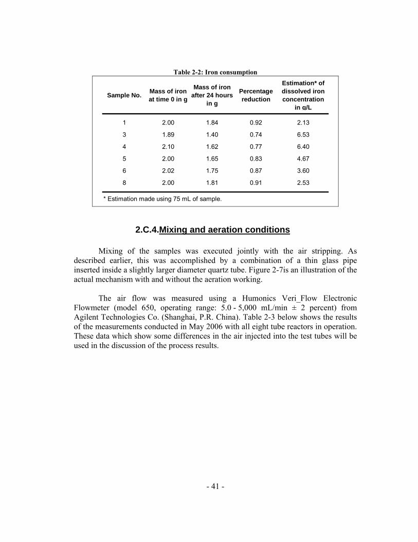
- 41 -

Table 2-2: Iron consumption

Sample No. Mass of iron at time 0 in g

Mass of iron after 24 hours

in g

Percentage reduction

Estimation* of dissolved iron concentration

in g/L

* Estimation made using 75 mL of sample.

3.60

8 2.00 1.81 0.91 2.53

6 2.02 1.75 0.87

6.40

5 2.00 1.65 0.83 4.67

4 2.10 1.62 0.77

2.13

3 1.89 1.40 0.74 6.53

1 2.00 1.84 0.92

2.C.4.Mixing and aeration conditions Mixing of the samples was executed jointly with the air stripping. As described earlier, this was accomplished by a combination of a thin glass pipe inserted inside a slightly larger diameter quartz tube. Figure 2-7is an illustration of the actual mechanism with and without the aeration working. The air flow was measured using a Humonics Veri_Flow Electronic Flowmeter (model 650, operating range: 5.0 - 5,000 mL/min ± 2 percent) from Agilent Technologies Co. (Shanghai, P.R. China). Table 2-3 below shows the results of the measurements conducted in May 2006 with all eight tube reactors in operation. These data which show some differences in the air injected into the test tubes will be used in the discussion of the process results.

- 42 -

Table 2-3: Air flow measurments

Flow path 05/03/06 05/04/06

Air flow in L/min

Date of measurement

1 0.138 0.13

2 0.101 0.11

3 0.093 0.109

4 0.054 0.067

5 0.152 0.196

6 0.202 0.338

7 0.206 0.435

8 0.08 0.089

Figure 2-7: Aeration System Off (left) and On (right)

2.C.5.Filtration Filtration was necessary to eliminate suspended solids such as iron particles in simulated leachate and any suspended solids from the real leachate. This process

- 43 -

simulated sedimentation or filtration in the field. Before analysis, all samples were filtered to remove suspended iron particles and precipitates using either syringe-less filters (see Figure 2-8) or vacuum filtration. In both cases, the filter pore size was 0.45μm. The syringe-less filters were manufactured by Whatman Inc. (Clifton, NJ) and the glass fiber filter used with the vacuum was from Pall Corporation (Ann Arbor, MI). The syringe filters were used for the intermediate and final monitoring experiments, where a small quantity (0.2 to 0.4 mL) of sample was necessary. The vacuum filtration was used at the end of treatment. This filtration technique required a large volume of sample, but the capacity of the test tubes allowed only one filtration. Vacuum filtration mainly was used for BOD5 experiments.

Figure 2-8: Syringe-less filter

- 44 -

CHAPTER 3: RESULTS AND DISCUSSION

- 45 -

3.A.Simulated leachate: individual scoping tests Table 3-1 summarizes the order of individual scoping tests on simulated leachate experiments.

Table 3-1: Order of execution of the simulated leachate experiments Experiment

Number Component tested Level

13 Conductivity & TDS Low

14 Lead Medium

11 BOD5 Low

12 Conductivity & TDS High

09 Ammonia Low

10 BOD5 High

07 BOD5 Medium

08 Ammonia Medium

05 Conductivity & TDS Medium

06 COD Medium

03 Ammonia High

04 COD High

01 Conductivity Test

02 COD Low

Beginning with COD, this section is presenting the results obtained during these experiments.

3.A.1.COD Experiments on Chemical Oxygen Demand were the first to be completed. Three scoping tests for COD have been performed. The initial concentrations were respectively 1.05, 3.30 and 10.90 g/L as O2 for the low, medium and high concentration levels.

3.A.1.a.Low concentration level The first experiment (experiment No. 02), performed on the low concentration level (1.05 g/L as O2), was monitored after two, four and twenty-four hours of treatment. It showed a best removal of 54 percents for the PIMA process at close-distance (6.3 cm), the concentration was reduced to 0.58 g/L as O2 after 24 hours. The IMA process, at mid-distance achieved a removal of 21 percents and

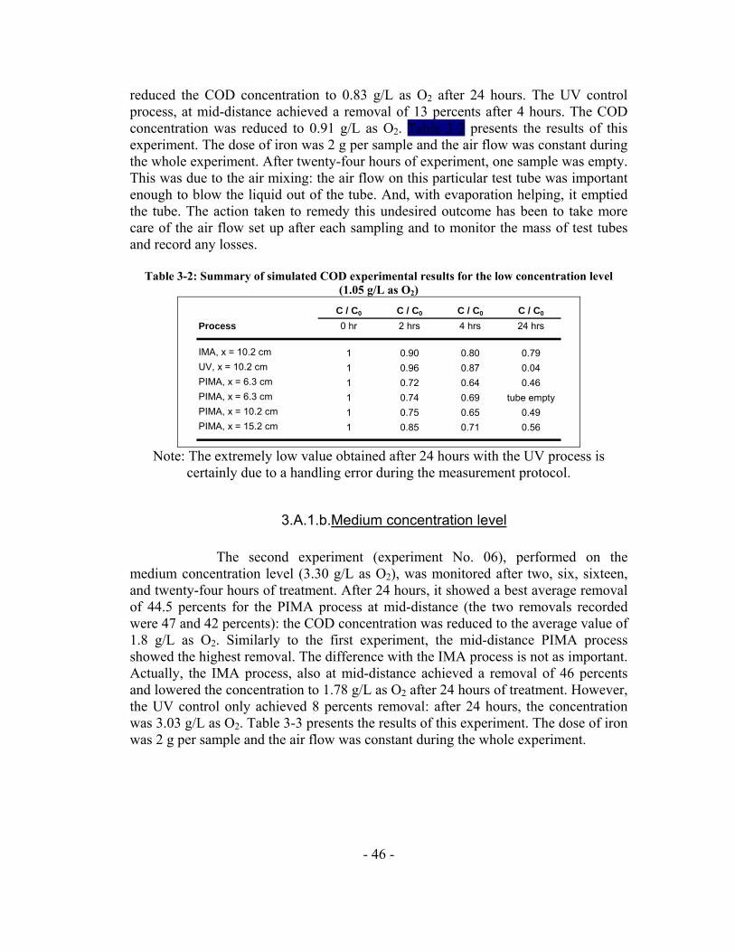
- 46 -

reduced the COD concentration to 0.83 g/L as O2 after 24 hours. The UV control process, at mid-distance achieved a removal of 13 percents after 4 hours. The COD concentration was reduced to 0.91 g/L as O2. Table 3-2 presents the results of this experiment. The dose of iron was 2 g per sample and the air flow was constant during the whole experiment. After twenty-four hours of experiment, one sample was empty. This was due to the air mixing: the air flow on this particular test tube was important enough to blow the liquid out of the tube. And, with evaporation helping, it emptied the tube. The action taken to remedy this undesired outcome has been to take more care of the air flow set up after each sampling and to monitor the mass of test tubes and record any losses.

Table 3-2: Summary of simulated COD experimental results for the low concentration level (1.05 g/L as O2)

C / C0 C / C0 C / C0 C / C0

Process 0 hr 2 hrs 4 hrs 24 hrs

1 0.90 0.80 0.791 0.96 0.87 0.041 0.72 0.64 0.461 0.74 0.69 tube empty1 0.75 0.65 0.491 0.85 0.71 0.56

UV, x = 10.2 cmIMA, x = 10.2 cm

PIMA, x = 6.3 cmPIMA, x = 6.3 cmPIMA, x = 10.2 cmPIMA, x = 15.2 cm

Note: The extremely low value obtained after 24 hours with the UV process is

certainly due to a handling error during the measurement protocol.

3.A.1.b.Medium concentration level The second experiment (experiment No. 06), performed on the medium concentration level (3.30 g/L as O2), was monitored after two, six, sixteen, and twenty-four hours of treatment. After 24 hours, it showed a best average removal of 44.5 percents for the PIMA process at mid-distance (the two removals recorded were 47 and 42 percents): the COD concentration was reduced to the average value of 1.8 g/L as O2. Similarly to the first experiment, the mid-distance PIMA process showed the highest removal. The difference with the IMA process is not as important. Actually, the IMA process, also at mid-distance achieved a removal of 46 percents and lowered the concentration to 1.78 g/L as O2 after 24 hours of treatment. However, the UV control only achieved 8 percents removal: after 24 hours, the concentration was 3.03 g/L as O2. Table 3-3 presents the results of this experiment. The dose of iron was 2 g per sample and the air flow was constant during the whole experiment.

- 47 -

Table 3-3: Summary of simulated COD experimental results for the medium concentration level (3.30 g/L as O2)

C / C0 C / C0 C / C0 C / C0 C / C0

Process 0 hrs 2 hrs 6 hrs 16 hrs 24 hrs

1 0.83 0.66 0.47 0.541 1.05 1.01 0.89 0.921 0.96 0.68 0.53 0.641 0.84 0.69 0.63 0.811 0.97 0.67 0.50 0.531 0.93 0.65 0.52 0.581 0.96 0.72 0.49 0.571 1.00 0.65 0.48 0.59

IMA, x = 10.2 cm

PIMA, x = 10.2 cmPIMA, x = 15.2 cmPIMA, x = 15.2 cm

UV, x = 10.2 cmPIMA, x = 6.3 cmPIMA, x = 6.3 cmPIMA, x = 10.2 cm

3.A.1.c.High concentration level The third experiment (experiment No. 04), performed on the high concentration level, was monitored after two, four, height, sixteen, and twenty-four hours of treatment. The best removal was also observed with the PIMA process. The percentage removal was about 40 percent, which represented 4.36 g/L. The UV control process achieved almost no removal. Confirming what occurred during the first two experiments, the IMA process gave similar results compared to the PIMA. Table 3-4 presents the results of this experiment. The dose of iron was 2 g per sample and the air flow was constant during the whole experiment.

Table 3-4: Summary of simulated COD experimental results for the high concentration level (10.90 g/L as O2)

C / C0 C / C0 C / C0 C / C0 C / C0 C / C0

Process 0 hr 2 hrs 4 hrs 8 hrs 16 hrs 24 hrs

1 1.03 0.87 0.74 0.61 0.581 0.97 1.05 0.99 0.97 0.981 0.92 0.86 0.76 0.65 0.601 0.98 0.85 0.73 0.99 0.641 0.93 0.83 0.75 0.63 0.591 0.95 0.91 0.79 0.81 0.971 0.99 0.85 0.73 0.80 0.621 0.98 0.87 0.69 0.57 0.58

IMA, x = 10.2 cmUV, x = 10.2 cm

PIMA, x = 15.2 cmPIMA, x = 15.2 cm



3.A.1.d.Summary The results of these three experiments are illustrated in Figure 3-1. It represents the average removal percentages of COD at different times without distinction of initial concentration. This graph clearly demonstrates that UV is far less efficient than IMA or PIMA. This fact is even more evident as the original

- 48 -

concentration increases. However, no major difference can be noticed between these two processes. A portion of the light emitted by the UV lamp is suspected to pass through the glass test tube. The reactor has been improved and thin shield has been added between the lamp and the IMA control test tube to prevent the visible radiation to irradiate the leachate. These three experiments showed that there is no benefit to extend the reaction time beyond 16 hours. Nevertheless, for all simulated leachate experiment, the process has been evaluated up to twenty-four hours. No pH adjustment was made, but it was recorded at each sampling time and stayed at an average of 5.5, independently of the KHP concentration. The temperature inside the cabinet was recorded and stayed stable over time. As it was simply monitored, no conclusion can be drawn on its influence on the process.

C / C0 versus Time

0.00

0.20

0.40

0.60

0.80

1.00

0 5 10 15 20 25

Time in hrs

C /

C0

UV, x = 10.2 cm IMA, x = 10.2 cm PIMA, x = 6.3 cm PIMA, x = 10.2 cm PIMA, x = 15.2 cm

Figure 3-1: Global summary of simulated COD experimental results

3.A.2.Conductivity and TDS The very first experiment (experiment No. 01) was held on conductivity. This was an experiment test, and the results are not exploitable (concentration only measured after 2 hours of treatment). Running this experiment was very useful to learn on the reactor and how to conduct the future experiments. Then, one experiment (experiment No. 05) on conductivity and TDS was completed. The initial concentrations were 16,250 μS/cm and 8.12 g/L respectively. This corresponds to the medium concentration level. The next two experiments were executed on the high (experiment No. 12 with initial concentrations of 81,625 μS/cm and 40.0 g/L) and low (experiment No. 13 with initial concentrations of 2,750 μS/cm and 0.83 g/L) levels.

3.A.2.a.Low concentration level

- 49 -

The experiment performed on the low concentration level, was monitored after two, six, sixteen and twenty-four hours of treatment. Initial concentrations were measured at the values of 2,750 μS/cm for conductivity and 830 mg/L for TDS. During this experiment, iron fibers were weighted before and after treatment. Results are shown in Table 3-5. After 24 hours of treatment, an average concentration of 4.3 g/L can be expected. This concentration is only expected because part of the lost iron is not dissolved but remains on the sludge at the bottom of the test tube. Figure 3-2 is showing the bottom sludge 5 minutes after removing the iron from the test tube. This explains the absence of conductivity removal for the IMA and PIMA processes: The decrease of conductivity due to the salt is compensated by the increase of conductivity due to the dissolving iron. What is more surprising is that the same trend is also observed in absence of iron (UV control process). No explanation has yet been found on this concern; but the evaporation of the liquid may be one of the reasons. Table 3-5 presents conductivity results of this experiment. The dose of iron was 2 g per sample and the air flow was constant during the whole experiment. No pH adjustment was made, but it was recorded at each sampling time and stayed at an average value of 6.0. For this experiment, the temperature was recorded using an additional test tube at mid-distance filled with water. Over time, it indicated a maximum temperature of 35°C. This value is more representative of the leachate temperature. As temperature was simply monitored, no conclusion can be drawn on its influence on the process.

Figure 3-2: Sludge deposit after 24 hours of experiment

- 50 -

Table 3-5: Summary of simulated conductivity experimental results for the low concentration level (2,750 μS/cm)

C / C0 C / C0 C / C0 C / C0 C / C0

Process 0 hr 2 hrs 6 hrs 16 hrs 24 hrs

1.00 1.27 1.00 1.03 1.061.00 1.03 0.97 0.97 1.031.00 1.00 1.06 1.30 1.421.00 1.03 1.00 1.06 1.121.00 1.06 1.06 1.21 1.301.00 1.06 1.06 1.18 1.151.00 1.06 0.97 0.94 1.03

IMA, x = 10.2 cmUV, x = 10.2 cm



The same conclusions than these concerning conductivity can be formulated concerning TDS. This is correlated to the relationship between conductivity and TDS discussed earlier. Table 3-6 presents the results of this experiment concerning TDS. Due to the sensitivity of the Pocket Pal TDS tester and to the dilution factor, TDS concentration readings vary only from 10 to 20 mg/L. This is the reason why the results presented range from 0 to 2.

Table 3-6: Summary of simulated TDS experimental results for the low concentration level (830 mg/L)

C / C0 C / C0 C / C0 C / C0 C / C0


1.00 2.40 1.00 1.00 1.001.00 1.00 1.00 1.00 1.001.00 0.00 1.00 2.00 2.001.00 1.50 1.00 2.00 2.001.00 2.00 1.00 2.00 2.001.00 1.50 1.00 2.00 2.001.00 2.00 1.00 1.00 2.00

IMA, x = 10.2 cmUV, x = 10.2 cm



3.A.2.b.Medium concentration level The second experiment, performed on the medium concentration level, was monitored after two, four, eight, sixteen and twenty-four hours of treatment. Initial concentrations were measured at the values of 16,250 μS/cm for conductivity and 8.12 g/L for TDS. Concerning conductivity, it is not surprising to observe a decrease during the first hours of treatment due to the salt removal. After the 8 hours, the PIMA process at mid-distance (10.2 cm) showed the greatest removal of 20 percent. As the treatment continues, the concentration of dissolved iron increases and so is the conductivity. Salt removal is hidden behind the iron dissolution. This explains the gain up to 38 percent of conductivity for the IMA and PIMA. Concerning the UV

- 51 -

control process, the same conclusion is drawn than during the low concentration level experiment. Table 3-7 presents the results of this experiment. The dose of iron was 2 g per sample and the air flow was constant during the whole experiment. No pH adjustment was made, but it was recorded at each sampling time and stayed at an average of 6.0. The temperature inside the cabinet was recorded and stayed stable over time at a value near 36°C. As it was simply monitored, no conclusion can be drawn on its influence on the process.

Table 3-7: Summary of simulated conductivity experimental results for the medium concentration level (16,250 μS/cm)

C / C0 C / C0 C / C0 C / C0 C / C0 C / C0


1.00 0.98 0.85 0.95 1.14 1.381.00 0.98 0.78 0.95 1.19 1.331.00 1.00 0.93 0.93 1.14 1.231.00 0.99 1.05 0.67 1.18 1.431.00 0.99 0.95 1.11 1.16 1.281.00 1.00 1.03 0.96 1.12 1.461.00 1.00 0.99 0.95 1.09 1.251.00 0.99 1.05 1.13 1.14 1.28


UV, x = 10.2 cmIMA, x = 10.2 cm


PIMA, x = 15.2 cm

The same conclusions than these concerning conductivity can be formulated concerning TDS. As was mentioned previously, this is correlated to the relationship between conductivity and TDS discussed earlier. Table 3-8 presents the results of this experiment concerning TDS. Table 3-8: Summary of simulated TDS experimental results for the medium concentration level

(8.12 g/L) C / C0 C / C0 C / C0 C / C0 C / C0 C / C0


1.00 0.92 0.85 0.92 1.03 1.331.00 0.92 0.85 0.92 0.92 1.331.00 0.92 0.88 0.85 0.62 1.231.00 0.92 1.00 0.62 0.62 1.331.00 0.92 0.92 1.08 0.72 1.231.00 0.92 0.85 0.92 1.03 1.441.00 0.92 0.92 0.92 1.03 1.231.00 0.92 1.00 1.03 1.13 1.23


UV, x = 10.2 cmIMA, x = 10.2 cm


PIMA, x = 15.2 cm

This second experiment was the occasion to verify the relations between conductivity and TDS. Using the 45 measurements made during the experiment, an average factor of 2.23 has been found between conductivity and TDS. This confirms the existence of a relation between the two factors, but does not validate the experimental relation proposed by Snoeyink and Jenkins (1980). However, verifying the accuracy of these equations is beyond the scope of the study.

- 52 -

3.A.2.c.High concentration level The experiment performed on the high concentration level, was monitored after two, six, sixteen and twenty-four hours of treatment. Initial concentrations were measured at the value of 81,625 μS/cm for conductivity and 40.00 g/L for TDS. Concerning conductivity, no consequential removal was observed. Conductivity value remained stable throughout the whole experiment. After the six first hours of treatment, the PIMA process achieved an average of 7 percent removal. This removal equaled to a decrease of 5,700 μS/cm. As the experiment continued, conductivity started to increase again. Contrary to the medium level experiment where conductivity increase was significant, the initial concentration of this high level experiment was too high to observe the same range of increase. Concerning the UV control process, as seen in the two previous experiments, conductivity remained stable. Table 3-9 presents the results of this experiment. The dose of iron was 2 g per sample and the air flow was constant during the whole experiment. No pH adjustment was made, but it was recorded at each sampling time and stayed at an average of 6.0. The temperature inside the cabinet was recorded and stayed stable over time at a value near 36°C. As it was simply monitored, no conclusion can be drawn on its influence on the process.

Table 3-9: Summary of simulated conductivity experimental results for the high concentration level (81,625 μS/cm)

C / C0 C / C0 C / C0 C / C0 C / C0


1.00 0.94 1.02 1.02 0.921.00 0.92 1.00 0.93 0.891.00 0.99 0.76 1.13 0.871.00 1.00 0.98 1.05 1.021.00 0.97 0.94 0.99 1.061.00 0.96 1.03 0.00 1.011.00 0.93 0.90 1.03 1.081.00 0.91 0.97 1.04 1.06


UV, x = 10.2 cmPIMA, x = 6.3 cmPIMA, x = 6.3 cmPIMA, x = 10.2 cm

IMA, x = 10.2 cm

The same conclusions than these concerning conductivity can be formulated concerning TDS. As was mentioned previously, this is correlated to the relationship between conductivity and TDS discussed earlier. Table 3-10 presents the results of this high level experiment concerning TDS.

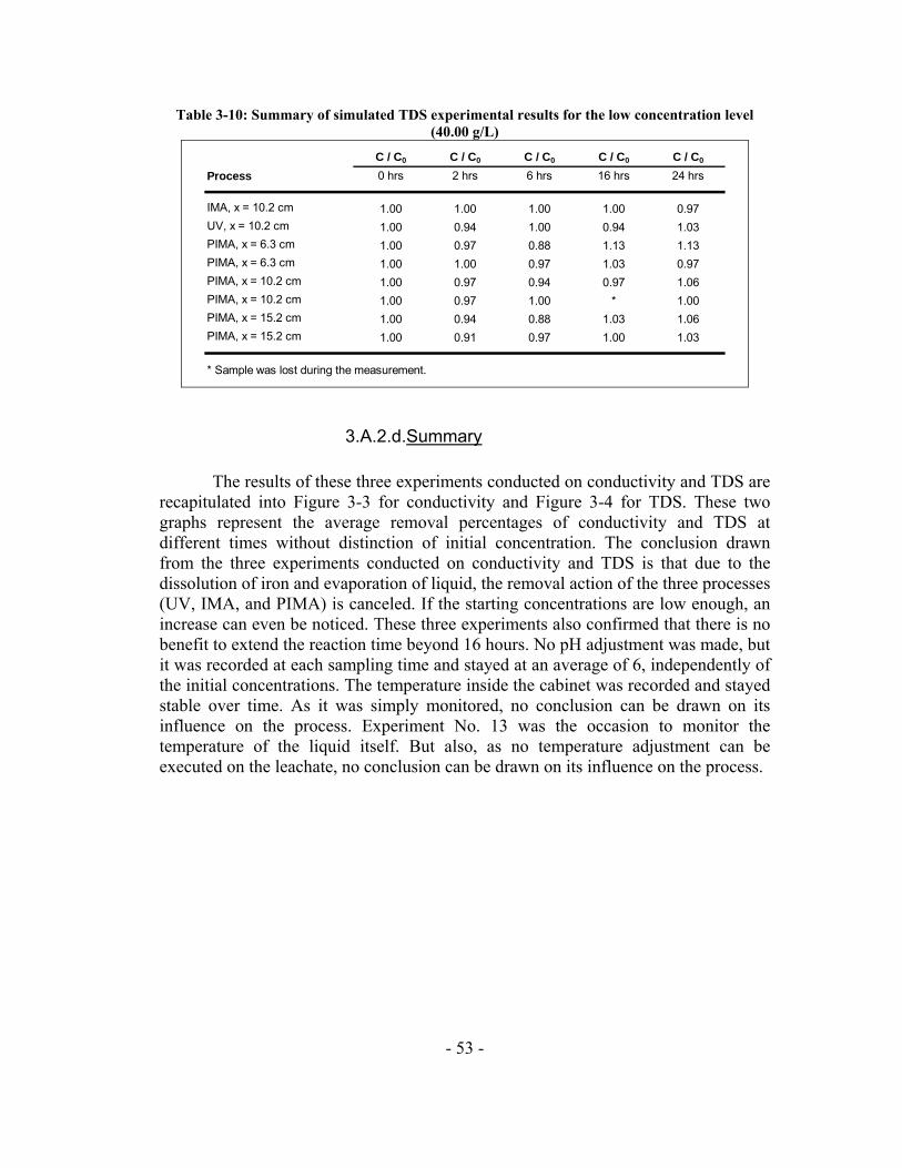
- 53 -

Table 3-10: Summary of simulated TDS experimental results for the low concentration level (40.00 g/L)

C / C0 C / C0 C / C0 C / C0 C / C0


1.00 1.00 1.00 1.00 0.971.00 0.94 1.00 0.94 1.031.00 0.97 0.88 1.13 1.131.00 1.00 0.97 1.03 0.971.00 0.97 0.94 0.97 1.061.00 0.97 1.00 * 1.001.00 0.94 0.88 1.03 1.061.00 0.91 0.97 1.00 1.03

* Sample was lost during the measurement.

IMA, x = 10.2 cm

PIMA, x = 15.2 cm

UV, x = 10.2 cmPIMA, x = 6.3 cmPIMA, x = 6.3 cmPIMA, x = 10.2 cmPIMA, x = 10.2 cmPIMA, x = 15.2 cm

3.A.2.d.Summary The results of these three experiments conducted on conductivity and TDS are recapitulated into Figure 3-3 for conductivity and Figure 3-4 for TDS. These two graphs represent the average removal percentages of conductivity and TDS at different times without distinction of initial concentration. The conclusion drawn from the three experiments conducted on conductivity and TDS is that due to the dissolution of iron and evaporation of liquid, the removal action of the three processes (UV, IMA, and PIMA) is canceled. If the starting concentrations are low enough, an increase can even be noticed. These three experiments also confirmed that there is no benefit to extend the reaction time beyond 16 hours. No pH adjustment was made, but it was recorded at each sampling time and stayed at an average of 6, independently of the initial concentrations. The temperature inside the cabinet was recorded and stayed stable over time. As it was simply monitored, no conclusion can be drawn on its influence on the process. Experiment No. 13 was the occasion to monitor the temperature of the liquid itself. But also, as no temperature adjustment can be executed on the leachate, no conclusion can be drawn on its influence on the process.

- 54 -

C / C0 versus Time

0.00

0.20

0.40

0.60

0.80

1.00

1.20

1.40

0 5 10 15 20 25

Time in hrs

C /

C0


Figure 3-3: Global summary of simulated conductivity experimental results

C / C0 versus Time

0.00

0.200.40

0.600.80

1.00

1.201.40

1.60

0 5 10 15 20 25

Time in hrs

C /

C0


Figure 3-4: Global summary of simulated TDS experimental results

3.A.3.BOD5 The three scoping experiment on Biological Oxygen Demand has been completed. The initial concentrations were respectively 1.05, 3.30 and 10.90 g/L as O2 for the low (experiment No. 11), medium (experiment No. 07) and high (experiment No. 10) concentration levels. As explained earlier, BOD5 experiments were monitored only after sixteen hours of treatment.

3.A.3.a.Low concentration level

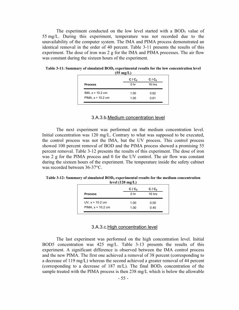
- 55 -

The experiment conducted on the low level started with a BOD5 value of 55 mg/L. During this experiment, temperature was not recorded due to the unavailability of the computer system. The IMA and PIMA process demonstrated an identical removal in the order of 40 percent. Table 3-11 presents the results of this experiment. The dose of iron was 2 g for the IMA and PIMA processes. The air flow was constant during the sixteen hours of the experiment.

Table 3-11: Summary of simulated BOD5 experimental results for the low concentration level (55 mg/L)

C / C0 C / C0

Process 0 hr 16 hrs

1.00 0.621.00 0.61

IMA, x = 10.2 cmPIMA, x = 10.2 cm

3.A.3.b.Medium concentration level The next experiment was performed on the medium concentration level. Initial concentration was 120 mg/L. Contrary to what was supposed to be executed, the control process was not the IMA, but the UV process. This control process showed 100 percent removal of BOD and the PIMA process showed a promising 55 percent removal. Table 3-12 presents the results of this experiment. The dose of iron was 2 g for the PIMA process and 0 for the UV control. The air flow was constant during the sixteen hours of the experiment. The temperature inside the safety cabinet was recorded between 36-37°C.

Table 3-12: Summary of simulated BOD5 experimental results for the medium concentration level (120 mg/L)

C / C0 C / C0

Process 0 hr 16 hrs

1.00 0.001.00 0.45

UV, x = 10.2 cmPIMA, x = 10.2 cm

3.A.3.c.High concentration level The last experiment was performed on the high concentration level. Initial BOD5 concentration was 425 mg/L. Table 3-13 presents the results of this experiment. A significant difference is observed between the IMA control process and the new PIMA. The first one achieved a removal of 38 percent (corresponding to a decrease of 119 mg/L) whereas the second achieved a greater removal of 44 percent (corresponding to a decrease of 187 m/L). The final BOD5 concentration of the sample treated with the PIMA process is then 238 mg/L which is below the allowable

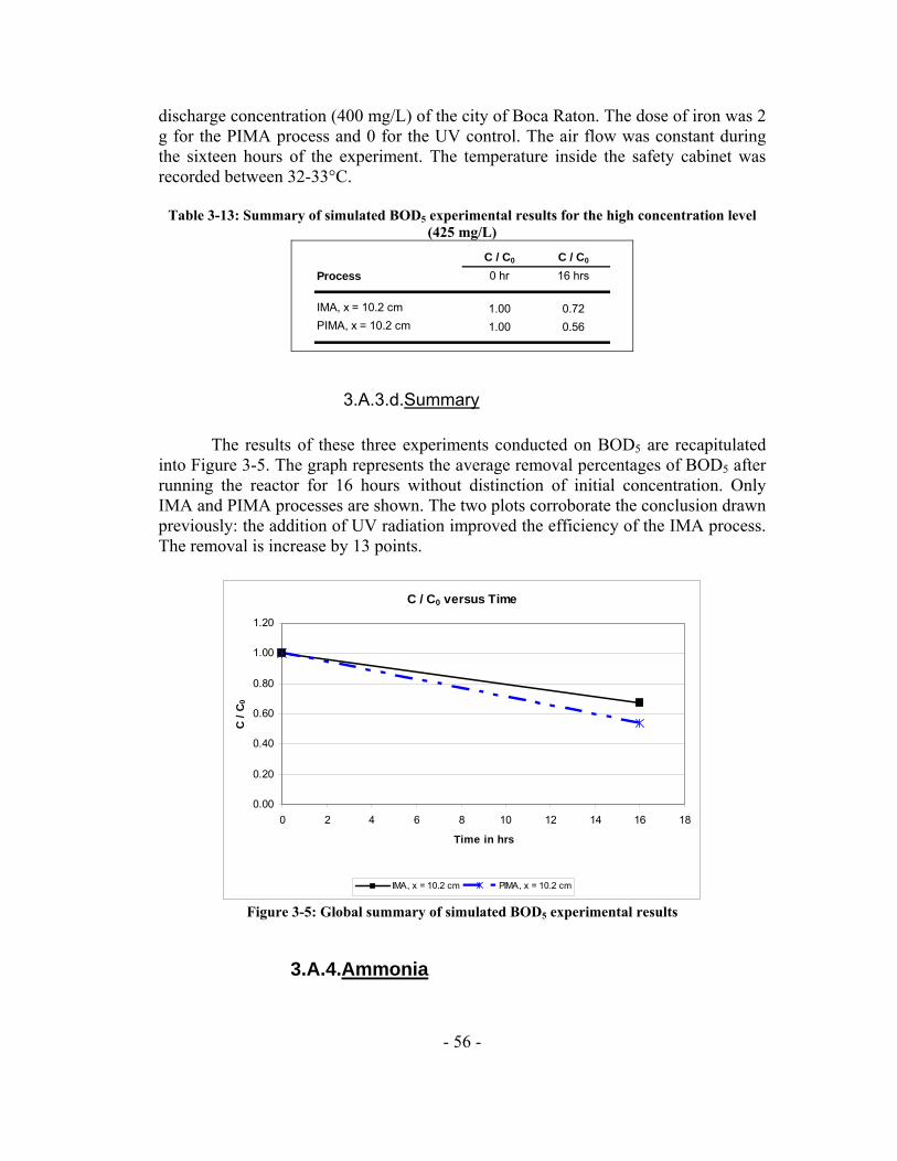
- 56 -

discharge concentration (400 mg/L) of the city of Boca Raton. The dose of iron was 2 g for the PIMA process and 0 for the UV control. The air flow was constant during the sixteen hours of the experiment. The temperature inside the safety cabinet was recorded between 32-33°C.

Table 3-13: Summary of simulated BOD5 experimental results for the high concentration level (425 mg/L)

C / C0 C / C0

Process 0 hr 16 hrs

1.00 0.721.00 0.56PIMA, x = 10.2 cm

IMA, x = 10.2 cm

3.A.3.d.Summary The results of these three experiments conducted on BOD5 are recapitulated into Figure 3-5. The graph represents the average removal percentages of BOD5 after running the reactor for 16 hours without distinction of initial concentration. Only IMA and PIMA processes are shown. The two plots corroborate the conclusion drawn previously: the addition of UV radiation improved the efficiency of the IMA process. The removal is increase by 13 points.

C / C0 versus Time

0.00

0.20

0.40

0.60

0.80

1.00

1.20

0 2 4 6 8 10 12 14 16 18

Time in hrs

C / C

0

IMA, x = 10.2 cm PIMA, x = 10.2 cm

Figure 3-5: Global summary of simulated BOD5 experimental results

3.A.4.Ammonia

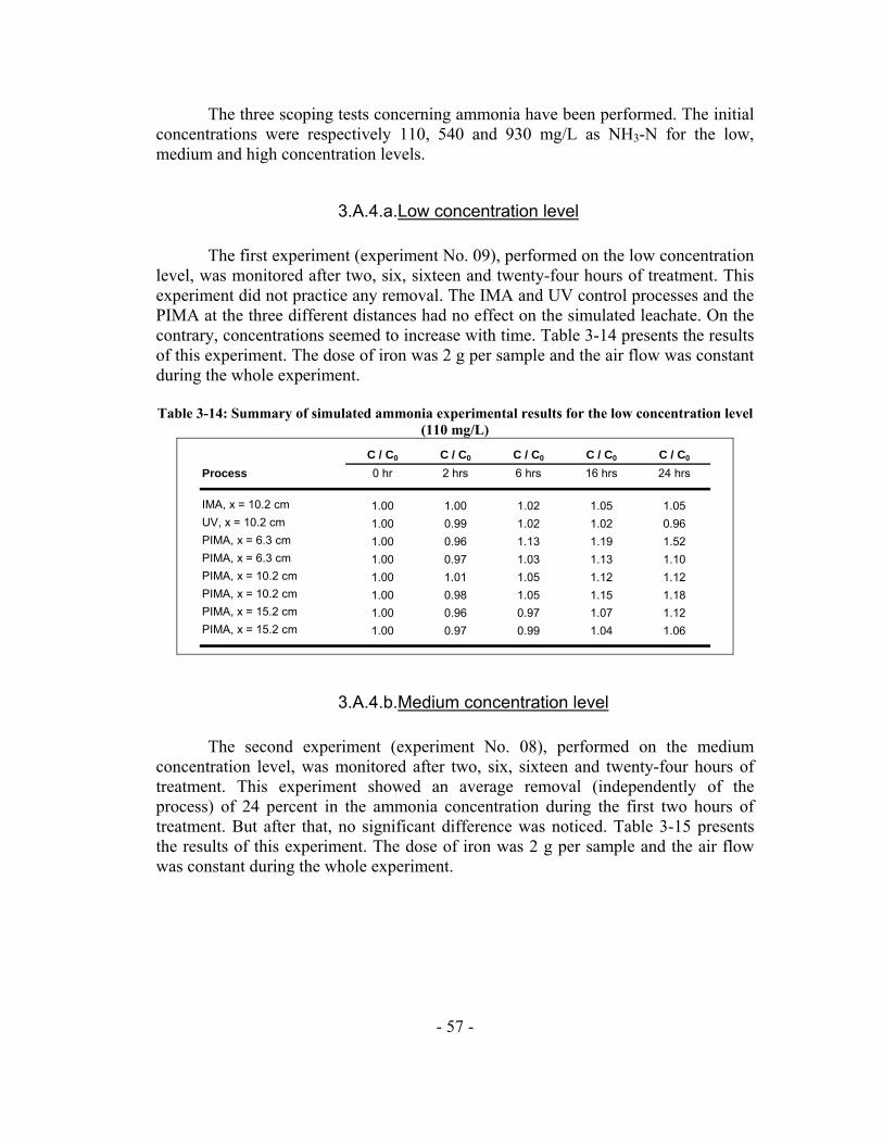
- 57 -

The three scoping tests concerning ammonia have been performed. The initial concentrations were respectively 110, 540 and 930 mg/L as NH3-N for the low, medium and high concentration levels.

3.A.4.a.Low concentration level The first experiment (experiment No. 09), performed on the low concentration level, was monitored after two, six, sixteen and twenty-four hours of treatment. This experiment did not practice any removal. The IMA and UV control processes and the PIMA at the three different distances had no effect on the simulated leachate. On the contrary, concentrations seemed to increase with time. Table 3-14 presents the results of this experiment. The dose of iron was 2 g per sample and the air flow was constant during the whole experiment. Table 3-14: Summary of simulated ammonia experimental results for the low concentration level

(110 mg/L)

C / C0 C / C0 C / C0 C / C0 C / C0


1.00 1.00 1.02 1.05 1.051.00 0.99 1.02 1.02 0.961.00 0.96 1.13 1.19 1.521.00 0.97 1.03 1.13 1.101.00 1.01 1.05 1.12 1.121.00 0.98 1.05 1.15 1.181.00 0.96 0.97 1.07 1.121.00 0.97 0.99 1.04 1.06


UV, x = 10.2 cmIMA, x = 10.2 cm


PIMA, x = 15.2 cm

3.A.4.b.Medium concentration level The second experiment (experiment No. 08), performed on the medium concentration level, was monitored after two, six, sixteen and twenty-four hours of treatment. This experiment showed an average removal (independently of the process) of 24 percent in the ammonia concentration during the first two hours of treatment. But after that, no significant difference was noticed. Table 3-15 presents the results of this experiment. The dose of iron was 2 g per sample and the air flow was constant during the whole experiment.

- 58 -

Table 3-15: Summary of simulated ammonia experimental results for the medium concentration level (540 mg/L)

C / C0 C / C0 C / C0 C / C0 C / C0


1.00 0.69 0.71 0.76 0.821.00 0.78 0.81 0.80 0.801.00 0.76 0.78 0.75 0.701.00 0.74 0.76 0.84 0.591.00 0.79 0.77 0.84 0.901.00 0.77 0.79 0.79 0.771.00 0.79 0.76 0.76 0.791.00 0.77 0.62 0.80 0.82

PIMA, x = 10.2 cm

IMA, x = 10.2 cmUV, x = 10.2 cm



PIMA, x = 10.2 cm

3.A.4.c.High concentration level The third experiment (experiment No. 03), performed on the high concentration level, was monitored after two, four and twenty-four hours of treatment. Exactly as the experiment No. 1, during this one, the three processes did not show any removal of ammonia. Table 3-16 presents the results of this experiment. The dose of iron was 2 g per sample and the air flow was constant during the whole experiment.

Table 3-16: Summary of simulated ammonia experimental results for the high concentration level (930 mg/L)

C / C0 C / C0 C / C0 C / C0

Process 0 hrs 2 hrs 4 hrs 24 hrs

1.00 1.01 1.03 1.081.00 0.98 0.97 1.121.00 0.92 0.91 0.991.00 1.00 0.99 1.101.00 0.97 1.06 1.031.00 0.96 0.99 0.87PIMA, x = 15.2 cm

UV, x = 10.2 cm


PIMA, x = 6.3 cm

IMA, x = 10.2 cm

3.A.4.d.Summary The experiments led on ammonia were not a complete success. Air stripping is known to remove ammonia from leachate, but during these three experiments, no significant changes have been sensed. Figure 3-6 is the illustration of this tendency. The pH was only monitored during the low and medium concentration level experiments. Initial pH was recorded at 6. At the exception of the UV control process where pH dropped to 5.5, pH remained stable along the two experiments. This acidic pH is the reason why air stripping did not achieve to remove ammonia. The air

- 59 -

stripping of ammonia from a liquid requires that the ammonia be present as a gas. Ammonia ions in leachate exist in equilibrium with gaseous ammonia as shown in the following equation:

++ +⎯→← HNHNH 34 As the pH is increased above 7, the equilibrium is shifted to the left and the ammonia ion is converted gaseous ammonia which may be removed by air stripping. Lime is usually used to increase the pH. However, during the three scoping experiments, pH was not adjusted but was recorded as acid. This is the reason why no removal was observed. Also the fact that ammonia gas is lighter than air does not encourage ammonia to strip and exit the test tube.

C / C0 versus Time

0.00

0.20

0.40

0.60

0.80

1.00

1.20

0 5 10 15 20 25

Time in hrs

C /

C0


Figure 3-6: Global summary of simulated ammonia experimental results

3.A.5.Lead At this time, experiments on lead have not been performed. Scoping tests for the other components showed that it was not necessary to pursue the experiment until twenty-four hours because the maximum removal efficiency was achieved well before. Consequently, the experiment will be run for a maximum of sixteen hours.

- 60 -

3.B.Simulated leachate: mixture scoping tests At this time, no experiment has been conducted on a simulated mixture of leachate components. After completing the lead experiments, this will be the following step.

- 61 -

3.C.Real leachate Also, no real leachate tests have been performed. They will be conducted after those for the simulated mixture.

- 62 -

CHAPTER 4: CONCLUSION AND RECOMMENDATIONS

- 63 -

After Year One, several conclusions can be drawn. First of all, leachate cannot be considered as a typical wastewater. The concentrations of the constituents are too elevated compared to a typical (or even high strength) municipal wastewater. As a result, leachate should not be handled as such. Nevertheless, some facilities are still not pre-treating their leachate. To remedy this issue, several options are available. Basics options based on physical and chemical characteristics of the leachate and subsequent treatment demonstrated interesting results for specific parameters. For instance, filtration showed excellent results on TDS but does not achieve a sufficient removal of COD; air stripping can only be used to remove ammonia. More developed techniques tend to be better alternatives. Based on the oxidation power of the hydroxyl radical OH•, Advanced Oxidation Processes and Energized Processes seemed to achieve better removal for several components simultaneously. Cost and the number of processes required to treat leachate are then reduced. These techniques employ hydrogen peroxide, ozone or UV to treat leachate. Iron Mediated Aeration and Photochemical Iron Mediated Aeration are two of these processes that initial studies showed promising results for soil, groundwater and wastewater contaminants. The goal of this research was to specifically examine the properties of the PIMA process on landfill leachate. To do so, a laboratory scale reactor was engineered and modified to run several tests at the same time. Two control tests (UV and IMA) and 6 PIMA tests at three different distances (and consequently three different UV exposures) were run simultaneously. The first step of the PIMA performance study was to generate simulated leachate and measure the removal power of this treatment method. For COD, the PIMA process managed a removal in the range of the other AOP processes (50-60%). Unexpectedly, air stripping (which occurs as a byproduct of circulation of air in the test chamber) by itself should have reduced the ammonia contained in leachate. However, no removal action was detected for ammonia. Test chamber geometry and pH effects are likely implicated. Regarding TDS and conductivity, the removal action is counterbalanced due to the dissolution of iron into the liquid phase. Later tests on the amount of dissolved iron will likely confirm this. For BOD5, PIMA showed encouraging removal power on the first scoping test. However, this experiment is not fully completed and during the month of October 2006, two more experiments will be performed on BOD5 and on TDS and conductivity. In Year Two, experiments on simulated mixtures and real leachate will be performed. This step is schedule to begin in November 2006. When these experiments are completed, real leachate samples will be tested.

- 64 -

Appendix A: Leachate Composition in Floridian landfills

Range 0.04 - 0.10Average < 0.04 < 0.04 0.06 < 0.04Range 13,200 - 15,200 3,100 - 8,400 2,600 - 9,500 6,500 - 8,600 3,200 - 12,100 1,000 - 14,200 1,245 - 95,000 2,320 - 7,370

Average 14,100 6,200 5,200 7,600 8,300 9,600 40,470 5,090Range

AverageRange 900 - 88,000 220 - 4,100

Average 27,690 2,770Range

AverageRange 1,070 - 2,584 522 - 827 242 - 440 902 - 1,616 416 - 1,208 10,530 - 13,960

Average 1,850 636 351 1,165 857 12,245Range 89 - 204 14 - 30 13 - 21 55 - 77 13 - 66

Average 140 22 15 66 42Range 7.3 - 7.6 6.5 - 7.4 6.8 - 7.5 7.3 - 7.8 7.5 - 7.9 7.3 - 7.8 2.0 - 11.3 6.5 - 8.1

Average 7.5 7.0 7.2 7.5 7.7 7.6 6.8 7.1

Landfill with leachate recycling

Landfill in a rural area

Capped landfill in a rural area

Landfill in a semi urban area Regional landfill

Landfill with enhanced biological

treatment in an urban area

Class I landfill at the Solid Waste Authority in Palm

Beach County

Class III landfill at the Solid

Waste Authority in Palm Beach

County

SOURCE

Lead in mg/L


TDS in mg/L


COD in mg/L

BOD5 in mg/L

pH

LANDFILL CHARACTERISTICS

Solid Waste Authority of Palm Beach County

Marnie L. Ward et al. (2002). “Determining Toxicity of Leachates from Florida Municipal Solid Waste Landfills Using a Battery of Tests Approach.” Environmental Toxicology , Vol. 17, Issue 3, p 258 - 266

TSS in mg/L

- 65 -

RangeAverage BDL 0.03 0.01 BDL 0.006 BDL BDLRange

AverageRange

AverageRange 800 - 1,400 4,000 - 8,000 3,500 - 8,000

Average 830 7,400 7,800 13,000 19,000Range 3 - 15 500 - 800 400 - 700

Average 28 940 710 1,300 1,300Range 55 - 150 1,500 - 5,000 1,000 - 2,500

Average 110 5,400 4,300Range

AverageRange

Average 7.1 8.0 7.7 7.3 7.5

Okeechobee County LandfillSt. Lucie County landfills

COD in mg/L

SOURCE St. Lucie County Glades Road Landfill Water Quality Report January 2005, prepared by CDM

St. Lucie County Baling & Recycling Facility Water Quality Report July 2005, prepared by CDM, Eric

Grotke

TDS in mg/L

TSS in mg/L

Okeechobee County 2nd 2005 Semi-annual Water Quality

Monitoring Report Berman Road Landfill, Leachate analysis report

by STL (Severn Trent) Denver


BOD5 in mg/L

pH

Lead in mg/L



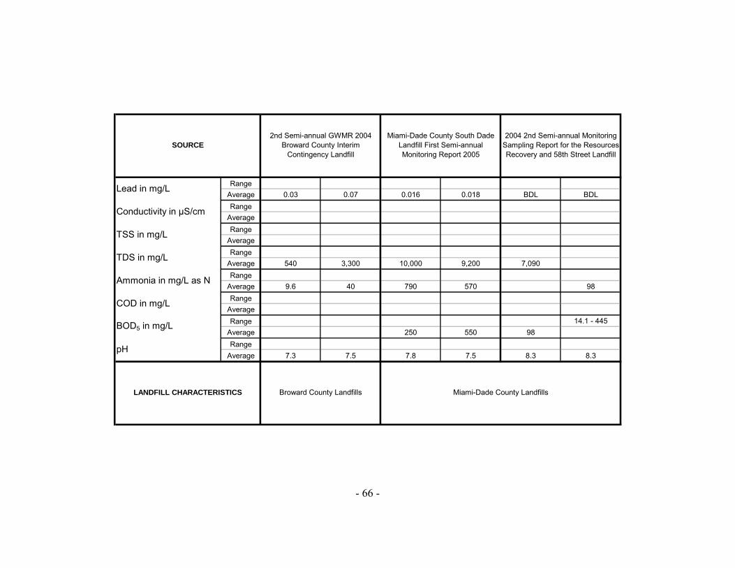
- 66 -

RangeAverage 0.03 0.07 0.016 0.018 BDL BDLRange

AverageRange

AverageRange

Average 540 3,300 10,000 9,200 7,090Range

Average 9.6 40 790 570 98Range

AverageRange 14.1 - 445

Average 250 550 98Range

Average 7.3 7.5 7.8 7.5 8.3 8.3

TSS in mg/L

2004 2nd Semi-annual Monitoring Sampling Report for the Resources Recovery and 58th Street Landfill

Broward County Landfills Miami-Dade County Landfills

pH

SOURCE

Lead in mg/L


TDS in mg/L


COD in mg/L

BOD5 in mg/L


2nd Semi-annual GWMR 2004 Broward County Interim

Contingency Landfill

Miami-Dade County South Dade Landfill First Semi-annual Monitoring Report 2005

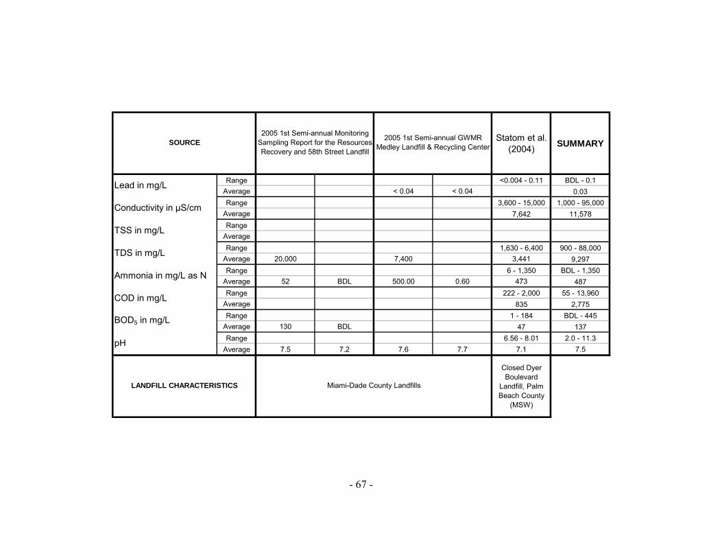
- 67 -

Statom et al. (2004) SUMMARY

Range <0.004 - 0.11 BDL - 0.1Average < 0.04 < 0.04 0.03Range 3,600 - 15,000 1,000 - 95,000

Average 7,642 11,578Range

AverageRange 1,630 - 6,400 900 - 88,000

Average 20,000 7,400 3,441 9,297Range 6 - 1,350 BDL - 1,350

Average 52 BDL 500.00 0.60 473 487Range 222 - 2,000 55 - 13,960

Average 835 2,775Range 1 - 184 BDL - 445

Average 130 BDL 47 137Range 6.56 - 8.01 2.0 - 11.3

Average 7.5 7.2 7.6 7.7 7.1 7.5

Closed Dyer Boulevard

Landfill, Palm Beach County

(MSW)


BOD5 in mg/L

pH

SOURCE

Lead in mg/L


TDS in mg/L


COD in mg/L

TSS in mg/L

2005 1st Semi-annual Monitoring Sampling Report for the Resources Recovery and 58th Street Landfill

2005 1st Semi-annual GWMR Medley Landfill & Recycling Center

Miami-Dade County Landfills

- 68 -

Appendix B

- 69 -

REFERENCES Akesson and Nilsson (1997). “Seasonal Changes of Leachate Production and Quality from Test Cells.” Journal of Environmental Engineering, Vol. 123, No. 9, p 892 - 900 Al-Yaqout et al. (2005). “Characteristics of Wastes, Leachate, and Gas at Landfills Operated in Arid Climate.” Practice periodical of hazardous, toxic, and radioactive waste management, Vol. 9, Issue 2, p 97 - 102 Amokrane et al. (1997). “Landfill leachates pretreatment by coagulation-flocculation.” Water research, Vol. 31, No. 11, p 2775 - 278 Anagiotou et al. (1993). “Leachate Treatment by Chemical and Biological Oxidation.” Journal of environmental science and health. Part A, Environmental science and engineering. Vol. 28, No. 1, p 21 - 36 Andreozzi et al. (1999). “Advanced oxidation processes (AOP) for water purification and recovery.” Catalysis Today, Vol. 53, p 51 - 59 APHA, AWWA and WEF (2005). Standard Methods for the Examination of Water & Wastewater, 21st Ed., American Public Health Association, Washington, DC. Englehardt et al. (2002), “In-situ chelation/reduction process for metals and radionuclides – Laboratory Study”, U.S. Department of Energy, Report Englehardt et al. (2005). “Options for Managing Municipal Landfill Leachate: Year 1 Development of Iron-Mediated Treatment Processes.” University of Miami Coral Gables, Internal Report. Environmental Health and Safety, (2004). “Chemical Hygiene Plan”, Florida Atlantic University, Boca Raton, http://www.fau.edu/ (February 24, 2006) EPA (2005). “Municipal Solid Waste in the United States - 2003 Facts and Figures.”, http://www.epa.gov (April 7, 2006) Esplugas et al. (2002) “Comparison of different advanced oxidation processes for phenol degradation.” Water Research, Vol. 36, p 1034 - 1042 FDEP (2002). “Solid Waste Management in Florida 2001-2002.”, http://www.dep.state.fl.us/ (April 19, 2006) Feitz et al. (1998) “Advanced oxidation processes and potential applications.” Water: Official Journal of the Australian Water and Wastewater Association. Vol. 26, No. 1, p 34 - 35

- 70 -

Geenens et al (2000). “Combined ozone-activated sludge treatment of landfill leachate.” Water Science and Technology, Vol. 44, No 2-3, p 359 - 365 Glaze et al. (1987). “Chemistry of Water Treatment Processes Involving Ozone, Hydrogen Peroxide and Ultraviolet Radiation.” Ozone Science and Engineering, Vol. 9, No 4, p 335 - 352 Gonze et al (2003). “High Frequency Ultrasound as a Pre-or a Post-Oxidation for Paper Mill Wastewaters and Landfill Leachate Treatment.” Chemical Engineering Journal, No. 92, p 215 - 225. Hickman (2003). American Alchemy – The History of Solid Waste Management in the United States, ForesterPress, Santa Barbara. Imai et al. (1998), “Effects of pre-ozonation in refractory leachate treatment by the biological activated carbon fluidized bed process.” Environmental Technology. Vol. 19, p 213 - 221 Ince (1998). “Light-enhanced chemical oxidation for tertiary treatment of municipal landfill leachate.” Water Environment Research, Vol. 70, No. 6, p 1161 - 1169 Kim et al. (1997). “Landfill leachate treatment by a photoassisted Fenton reaction.” Water science and technology, Vol. 35, No 4, p 229 - 248 Kjeldsen et al. (2002). “Present and Long-Term Composition of MSW Landfill Leachate: A Review.” Critical Reviews in Environmental Science and Technology, Vol. 32, No. 4, p 297 - 336 Loizidou et al. (1992), “Physical Chemical Treatment of Leachate from Landfill.” Journal of environmental science and health. Part A, Environmental science and engineering. Vol. 27, No. 4, 1059 - 1082 Loizidou et al. (1993). “Application of Chemical Oxidation for the Treatment of Refractory Substances in Leachates.” Journal of environmental science and health. Part A, Environmental science and engineering. Vol. 28, No. 2, p 385 - 402 Lopez et al. (2004). “Fenton's pre-treatment of mature landfill leachate.” Chemosphere. Vol. 54, No. 7, p 1005 - 1010 Meeroff et al. (2006). “Iron-Mediated Aeration: Evaluation of Energy-Assisted Enhancement for In Situ Subsurface Remediation.” Journal of Environmental Engineering, Vol. 132, No. 7, p 747 - 767

- 71 -

Metcalf and Eddy (2003). Wastewater Engineering, Treatment and Reuse, 4th Ed., McGraw-Hill Companies, New York. Monje-Ramirez and Orta de Velasquez (2004). “Removal and transfor-mation of recalcitrant organic matter from stabilized saline landfill leachates by coagulation-ozonation coupling processes.” Water Research, Vol. 38, p 2359 - 2367 Morris et al. (2003). “Findings from long-term monitoring studies at MSW landfill facilities with leachate recirculation.” Waste Management, Vol. 23, p 653 - 666 Munter et al. (2001). “Advanced Oxidation Processes (AOPs): Water Treatment Technology for the Twenty-first Century.” Kemia. Kemi., Vol. 28, Part 5, p 354 - 362 O’Leary et al. (1995). “Decision Maker’s Guide to Solid Waste Management, Volume II, (EPA 530-R-95-023)”, http://www.epa.gov (April 7, 2006) Oweis and Kehra (1998). Geotechnology of Waste Management, 2nd Ed., PWS Publishing Company, Boston. Papadopoulos et al. (1996). “Studies on the use of clinoptilolite for ammonia removal from leachates.” Journal of environmental science and health. Part A, Environmental science and engineering, Vol. 31, No. 1, p 211 - 220 Pohland and Harper (1986). Critical Review and Summary of Leachate and Gas Production From Landfills. EPA 600/2-86/073, USEPA. Qasim and Chiang (1994). Sanitary landfill leachate – Generation, Control and Treatment. CRC Press, Boca Raton. Reinhart and Townsend (1998). Landfill Bioreactor Design & Operation, Lewis Publishers, Boca Raton. Reinhart and Grosh (1998). “Analysis of Florida MSW landfill leachate quality.” Florida Center for Solid and Hazardous Management, Report #97-3 Shu et al. (2006). “Treatment of MSW landfill leachate by a thin gap annular UV/H2O2 photoreactor with multi-UV lamps.” Journal of Hazardous Materials, Vol. 129, No 1, p 73 – 79 Silva et al. (2003). “Treatment and detoxification of a sanitary landfill leachate.” Chemosphere, Vol. 55, p 207 - 214 Slomczynska et al. (2004). “Effect of advanced oxidation processes on the toxicity of municipal landfill leachates.” Water Science and Technology, Vol. 49, No. 4, p 273 - 277

- 72 -

Snoeyink and Jenkins (1980). Water Chemistry, John Wiley & Sons, New York. State of Florida (). “Florida Administrative - Code Chapter 62 – Department of Environmental Protection”, http://www.myflorida.com/ (February 23, 2006) Statom et al. (2004). “Temporal changes in leachate chemistry of a municipal solid waste landfill cell in Florida, USA.” Environmental Geology, Vol. 45, p 982 - 991 Steensen (1997). “Chemical oxidation for the treatment of leachate - Process comparison and results from full-scale plants.” Water science and technology, Vol. 35, No 4, p 249 - 256 Street et al. (2002). “Lead Removal from Synthetic Leachate Matrices by a Novel Ion-Exchange Material.” Journal of the Air & Waste Management Association Vol. 52, No. 9, p 1075 - 1082 Tammemagi (1999). The Waste Crisis - Landfills, incinerators, and the search for a sustainable future, Oxford, New York Tatsi et al. (2003). “Coagulation–flocculation pretreatment of sanitary landfill leachates.” Chemosphere, Vol. 53, p 737 - 744 Tchobanoglous and Kreith (2002). Handbook of Solid Waste Management, 2nd Ed., McGraw-Hill Handbooks, New York. Ward et al. (2002). “Determining Toxicity of Leachates from Florida Municipal Solid Waste Landfills Using a Battery of Tests Approach.” Environmental Toxicology, Vol. 17, Issue 3, p 258 - 266 Westlake (1995). Landfill Waste Pollution and Control, Albion Publishing, Chichester (England). Wu et al. (2004). “Treatment of landfill leachate by ozone-based advanced oxidation processes.” Chemosphere, Vol. 54, p 997 - 1003 Youcai et al. (2002). “Treatment of Leachate by Aged-Refuse-Based Biofilter.” Journal of Environmental Engineering, Vol. 128, No. 7, p 662 - 668.

http://en.wikipedia.org

investigation of energized options for leachate …

Documents