investigation of design parameters for increased solar ... · investigation of design parameters...
TRANSCRIPT

Investigation of Design Parameters for Increased Solar Potential of
Dwellings and Neighborhoods
Caroline Hachem
A Thesis
In the Department
of
Building, Civil, and Environmental Engineering
Presented in Partial Fulfillment of the Requirements
For the Degree of
Doctor of Philosophy (Building Engineering) at
Concordia University
Montreal, Quebec, Canada
September 2012
© Caroline Hachem, 2012

ii

iii
Abstract
Investigation of Design Parameters for Increased Solar Potential of
Dwellings and Neighborhoods
Caroline Hachem, PhD
Concordia University, 2012
Neighborhoods can be designed to achieve net-zero energy consumption by
addressing key design parameters for optimal solar collection, while allowing flexibility
of building designs.
The current study comprises a comprehensive investigation of key parameters
of dwelling shapes and neighborhood patterns for increased solar potential. Key
findings and recommendations related to the solar potential and energy consumption of
these dwellings and their assemblages are presented. Solar potential include the capture
of solar radiation incident on, and transmitted by windows of near equatorial facing
facades, and energy generation by building integrated photovoltaic systems covering
complete near equatorial facing roof surfaces. The design parameters studied include
geometric shapes of individual units, density of units and site layouts. Dwelling shapes
include basic geometries and variations on these geometrical shapes. Density effect is
analyzed through different assemblages of detached and attached housing units, as well
as of parallel rows of units. Site layouts include straight road configurations and semi-
circular road patterns, with the curve facing south or north. Roof designs are

iv
investigated independently to explore concepts offering an increased electrical/ thermal
energy generation potential of integrated photovoltaic/thermal systems.
The analysis employs the EnergyPlus simulation package to simulate
configurations consisting of combinations of values of parameters in order to assess the
effects of these parameters on the solar potential, as well as heating and cooling
demand/consumption of dwellings and neighborhoods. Effects are evaluated as the
change of the energy generation and energy demand/consumption, relative to reference
configurations. The reference shape is a rectangle, the reference density is detached
units and the reference layout is a straight road. The weather data for Montreal, Canada
(45°N) are employed to represent a northern mid-latitude climate zone.
An evaluation procedure is proposed as decision-aiding tool to assess the
performance of design alternatives. The evaluation is based on design parameter effects
and weights assigned to different performance criteria. A holistic design methodology
is developed to support the design and analysis of solar optimized residential
neighborhoods. This methodology may be employed to assist the design of net-zero
energy communities while allowing for different dwelling shapes, roads and density
patterns.

v
Acknowledgments
I would like to express my deepest gratitude to my supervisors, Dr. Andreas
Athienitis and Dr. Paul Fazio, for their invaluable support and guidance. Through their
material support and encouragement I was exposed to a broad range experiences
including participation in numerous international conferences, becoming a member of
the international energy agency (IEA) task 41- Solar Energy and Architecture, and
assisting in different workshops and seminars.
I convey my sincere and deep gratitude to Dr. Ariel Hanaor, for his guidance,
his support and his patience in revising and editing this work.
Recognition is due to a great number of individuals in Concordia University,
particularly to Mrs. Lyne Dee for her valuable assistance, Mrs. Olga Soares, and the
administrative staff in general.
This project was made possible through the major Alexander Graham Bell
Scholarship of the Natural Sciences and Engineering Research Council of Canada
(NSERC), ASHRAE grant-in aid award and from NSERC discovery grants held by Dr.
Athienitis and Dr. Fazio and by the Faculty of Engineering and Computer Science of
Concordia University. Their financial supports to this project are greatly appreciated.
This work was also partly supported by the NSERC Smart Net-zero Energy
Buildings Strategic Research Network.

vi
Table of Contents
List of Figures ...........................................................................................................................................ix
List of Tables .......................................................................................................................................... xii
Nomencatures ......................................................................................................................................... xiv
Introduction ............................................................................................................................................... 1
Chapter I: Literature Survey ...................................................................................................................... 8
1.1. Energy Efficient and Net Zero Energy Housing ................................................................................. 8
1.1.1. Energy Efficient Houses ......................................................................................... 10
1.1.2 Active Solar Technologies ....................................................................................... 19
1.2.Energy Performance of Buildings and Neighborhoods ..................................................................... 29
1.2.1. Energy and Building Shapes .................................................................................. 30
1.2.2. Effects of Urban Design ......................................................................................... 34
1.2.3. Case studies ............................................................................................................ 39
1.3. Tools ................................................................................................................................................. 46
1.3.1. Modeling of Net-Zero Energy Solar Houses ............................................................... 46
1.3.2.Tools for Simulations of Urban Areas .......................................................................... 48
Chapter II: Design and Methodology of the investigation ....................................................................... 51
2.1. Outline of the Investigation .............................................................................................................. 51
2.1.1 Background................................................................................................................... 51
2.1.2. Objectives and Scope ................................................................................................... 54
2.2. Methodology ..................................................................................................................................... 56
2.2.1. Shape Study ................................................................................................................. 57
2.2.2. Neighborhood Study .................................................................................................... 60
2.2.3. Roof Study ................................................................................................................... 64
2.2.4. Design Methodology for Solar Neighborhoods ........................................................... 66
2.3. Tools ................................................................................................................................................. 67
2.3.1. Selection of Simulation Software ................................................................................ 67
2.3.2. Modeling and Simulations ........................................................................................... 69
Chapter III: Dwelling Shapes .................................................................................................................. 73
3.1. Shape Design and Investigation ........................................................................................................ 73
3.1.1 Basic Design Assumptions ........................................................................................... 74
3.1.2 Shape of Dwelling Units ............................................................................................... 75
3.1.3 Parametric Investigation ............................................................................................... 80
3.2 Presentation and Analysis of Results ................................................................................................. 85
3.2.1. Effects of Basic Shape Design ....................................................................... 86
3.2.2. Variations of Basic Shapes ........................................................................... 92

vii
3.2.3. Energy Balance of Basic Shapes .................................................................. 103
Chapter IV: Neighborhood design ......................................................................................................... 106
4.1 Design Parameters ........................................................................................................................... 106
4.1.1. Neighborhood Characteristics ................................................................................... 107
4.1.2 Shading Effects ........................................................................................................... 108
4.1.3 Neighborhood Design Parameters and their Values ................................................... 110
4.1.4 Summary of Parametric Investigation ........................................................................ 116
4.2 Presentation and Analysis of Results ............................................................................................... 118
4.2.1. Shading Effect ........................................................................................................... 119
4.2.2 Density Effect ............................................................................................................. 124
4.2.3. Effect of Site Layout.................................................................................................. 134
4.2.4. Evaluation of Energy Balance of Neighborhoods .................................................... 143
Chapter V: Roofs ................................................................................................................................... 146
5.1. BIPV/T systems .............................................................................................................................. 147
Approximate Model ............................................................................................................. 147
5.2. Basic Surface Parameters and their Effect ...................................................................................... 153
5.2.1. Effect of Tilt Angle.................................................................................................... 153
5.2.2. Effect of Orientation Angle ....................................................................................... 154
5.2.3. Combination of Tilt and Orientation Angles ............................................................. 157
5.3. Design of Roofs .............................................................................................................................. 158
5.3.1. Hip Roofs................................................................................................................... 159
5.3.2. Advanced Roof Design .............................................................................................. 160
5. 3.3 Redesign of Units ...................................................................................................... 164
5.4 Presentation and Analysis of Results ............................................................................................... 165
5.4.1. Roof Morphology Effect ........................................................................................... 165
5.4.2 Redesign of Units ....................................................................................................... 172
5.4.3 Evaluation of Energy Balance .................................................................................... 173
Chapter VI: Guidelines for Design of Solar Housing Units and Neighborhoods ................................. 176
6.1. Summary of Design Parameters and their Effects .......................................................................... 176
6.1.1. Shape Parameters ....................................................................................................... 176
6.1.2. Neighborhood Parameters ......................................................................................... 180
6.1.3. Roof Parameters ....................................................................................................... 182
6.1.4. Tables of Performance ............................................................................................... 183
6.1.5 Design Considerations and Evaluation of Energy Performance ................................ 191
6.2. Solar Neighborhood Design Methodology ..................................................................................... 203
Chapter VII: Conclusion ........................................................................................................................ 215
References ............................................................................................................................................. 230
Appendix A............................................................................................................................................ 242
Appendix B ............................................................................................................................................ 244

viii
Appendix C ............................................................................................................................................ 248
Glossary ................................................................................................................................................. 258

ix
List of Figures
Figure (i), Energy use per sector in Canada, based on data by NRCan (2010) .............................................. 1
Figure (ii), Tree-Diagram representing the investigation of design parameters ............................................ 7
Figure 1.1, Schematic illustrating major principles of a net –zero energy solar house for a cold
(relatively sunny) climate. ............................................................................................................................. 10
Figure 1.2 Energy use in residential buildings, based on data by NRCan (2010)... ..................................... 16
Figure 1.3, (a) Shingle PV, (b) PV Tiles (c) PV slates (Uni-Solar, 2011), (d) PV laminates (Solar
Power Panels, 2011). ..................................................................................................................................... 25
Figure 1.4, (a) Solar sandwich (Best Solar Energy, 2011), b) solar roof system (Systaic, 2011). ................. 25
Figure 1.5, (a) GreenPix Media Wall, (Beijing, China (© Simone Giostra & Partners/Arup); (b)
Solar decathlon (façade from Onyx). . .......................................................................................................... 26
Figure 1.6, (a) PV panels as window shutters, (Colt international, 2011); (b) Solar awnings, (Solar
Awning inbalance-energy.co.uk). .................................................................................................................. 27
Figure 1.7, PV cost index per cumulative production (Breyer and Gerlach, 2010). ...................................... 28
Figure 1.8, Aerial view of the Clarum houses (Clarum houses, 2003).. ........................................................ 40
Figure 1.9, Solarsiedlung am Schlierberg, Freiburg (Breisgau) (a) view of muli-story buildings and
terrace houses, of Mixed-function development, (b) plan view, (c) detail of the overhang of a terrace
house, (d) terrace house (Hagemann, 2007). ................................................................................................. 41
Figure 1.10, PV integration in Nieuwland, (a) on the roof of a parking lot; (b) in sport complex, (c)
noise wall houses, (d) Prefab PV roofs (PV UPSCALE: Nieuwland, 2008). ................................................ 42
Figure 1.11 Jo-Town Kanokodai (MSK corporation, IEA PVPS-Task 10: Japan: Jo-Town
Kanokodai). ................................................................................................................................................... 43
Figure 2.1, Basic shapes. .............................................................................................................................. 58
Figure 2.2, Shape parameters. ...................................................................................................................... 59
Figure 2.3, Hip roof of a rectangular plan layout. ......................................................................................... 59
Figure 2.4, Roof shapes. ............................................................................................................................... 60
Figure 2.5, Overall site designs ..................................................................................................................... 62
Figure 2.6, Illustration of the density parameters. ......................................................................................... 63
Figure 2.7, Sample neighborhood configurations.......................................................................................... 63
Figure 2.8, Sample modified roof shapes for rectangular housing unit: a) split surface; b) folded
plate. ............................................................................................................................................................. 66
Figure 3.1, Basic shapes. ............................................................................................................................... 77
Figure 3.2, Roof layouts of basic designs: a) Single ridge design for convex shapes; b) Double ridge
designs in L, T; c) Roofs of U and H shapes. ............................................................................................... 80
Figure 3.3, Irregular roof shapes and PV integration. PV integrated surfaces are shown hatched. a)
and b) represent roofs of V-WS60- variant and obtuse angle O-S, c) and d) represent V-EN60 and
O-N.Basic shapes. ......................................................................................................................................... 84
Figure 3.4, Transmitted radiations of windows in south façades for a WDD and for a SDD. ...................... 87
Figure 3.5, Window annual heat gain of all shapes associated with different south window areas.. ............ 88
Figure 3.6, WDD peak electricity generation and annual electricity generation for all basic shapes ........... 89

x
Figure 3.7, Correlation between building envelope area and heating load for varying ratios of
window areas.. ............................................................................................................................................... 90
Figure 3.8, Effect of window size on annual energy consumption for heating of basic shapes ................... 92
Figure 3.9, Relation between heating and cooling loads and aspect ratio of rectangular shape.. .................. 93
Figure 3.10, Effect of orientation on transmitted radiation over a summer and winter design day
(SDD and WDD) ........................................................................................................................................... 94
Figure 3.11, Heating load of rectangular units with various orientations.. .................................................... 95
Figure 3.12, Annual energy production of selected L variants, (a) South Facing (V-ES and V-WS),
(b) North Facing (V-EN and V-WN). ......................................................................................................... 100
Figure 3.13, electricity generation for L shape with wing rotation (kW/m2), (a) WDD, (b) SDD. ............ 102
Figure 3.14, Annual heating and cooling of selected L and L variant shapes (a) South facing, (b)
North facing................................................................................................................................................. 103
Figure 3.15, Energy use and energy supply of all basic shapes. ................................................................. 105
Figure 4.1, POA concept, shading and shaded units are represented by solid colour; shaded unit is in
the centre of the circle; (a) and (b) single shading unit with different , (c) and (d) two shading units ........ 109
Figure 4.2, 3-D view of the POA concept, (a) one shaded unit, (b) 2 shaded units .................................... 110
Figure 4.3, variation of site I, (a) south facing rectangle, (b) rectangles oriented to the street, (c) L-
variants (V) ................................................................................................................................................. 111
Figure 4.4, Configurations of shapes in different site layouts: a) site I; b) Site II; c) Site III.. ................... 112
Figure 4.5, Illustration of the POA concept for L variant in site II ............................................................. 112
Figure 4.6, Attached units in sites I, II and III. Site I: a) rectangular, b) L shape, c) L variants; Site
II: d) trapezoid; e) obtuse-angle; f) L variants. Site III: g) trapezoid; h) obtuse-angle; i) L variants .......... 114
Figure 4.7, row configurations of all studied shapes; (a) detached configurations; (b) attached
configurations. ............................................................................................................................................. 116
Figure 4.8, Shading effect on annual solar radiation of a rectangular shape, (a) single shading unit-
radiation as function of POA, (b) single shading unit- radiation as function of distance (d), (c) two
shading units- radiation as function of POA, (d) two shading unit- radiation as function of distance
(d) ................................................................................................................................................................ 121
Figure 4.9, Shading effect on heating load of rectangular shape, a) single shading unit- heating load
as function of POA, (b) single shading unit- heating load as function of distance (d), (c) two shading
units- heating load as function of POA, (d) two shading unit- heating load as function of distance (d) ..... 123
Figure 4.10, Comparison of heating and cooling demand between isolated units and detached units
in a neighborhood. ....................................................................................................................................... 127
Figure 4.11, Heating consumption at different spacing between units ....................................................... 128
Figure 4.12 Reduction in transmitted radiation due to row effect for WDD U1, U2 and U3 are the
units of the shaded row, U2 is the mid unit: a) Effect on selected configurations at 5m row
separation; b) Effect on detached rectangular units, at separations of 5, 10 and 20 m ................................ 130
Figure 4.13, Detached units (a) Heating load of two rows relative to isolated rows, (b) Heating load
of the two rows of detached units ................................................................................................................ 132
Figure 4.14, Comparison of the row effect in site I ‒ R1 exposed row, R2 obstructed row: (a)
Comparison to isolated row, (b) Heating loads of the two rows ................................................................. 133
Figure 4.15, Ratio of heating load of the obstructed row to the unobstructed row as function of the
minimal distance required to avoid shading ............................................................................................... 134
Figure 4.16, Comparisons of heating/ cooling loads and land use area of all configurations of the
inclined road sites. ....................................................................................................................................... 137

xi
Figure 4.17, Hourly electricity generation (from 4-6 AM to 6-8 PM) (kW) for site II, on a WDD: a)
on the total south roof of attached rectangular (trapezoid); b) on the hip of L variants of detached L
variants; c) on the hip of L variants of attached L variants ......................................................................... 142
Figure 4.18, Heating and cooling loads of sites II and III relative to site I ................................................. 143
Figure 4.19, Energy demand and production for isolated units of different shapes: a) Shapes of sites
I and II; b) Shapes of site III ........................................................................................................................ 144
Figure 5.1, a) Cross-section illustrating an open loop BIPV/T system , b) schematic illustrating the
thermal network in one control volume of the BIPV/T system ................................................................. 149
Figure 5.2, a) Qu/Qe for 45° tilt angle roof for one sunny day of each month, over a year; b) Qu/Qe
for WDD of roofs with different tilt angles ................................................................................................. 152
Figure 5.3, Relation beteen air velocity and the average air change temperature in the cavity (ΔT),
on a WDD. .................................................................................................................................................. 152
Figure 5.4, Monthly electricity generation for different tilt angles ............................................................. 154
Figure 5.5, Effect of the angle of orientation on: (a) the electricity generation, (b) heat generation
over the period between mid-October and mid-April. ................................................................................. 155
Figure 5.6, Effect of the angle of orientation on the monthly electricity generation of the BIPV/T
systems. ....................................................................................................................................................... 156
Figure 5.7, Effect of the angle of orientation on the electricity generation, (a) 30° for the WDD, (b)
60° for the WDD, (c) 30° for the SDD, (d) 60° for the SDD.. .................................................................... 157
Figure 5.8, Ratio of energy generation of different configurations to south facing BIPV/T system
with 45 ° tilt angle. ...................................................................................................................................... 158
Figure 5.9, Illustration of hip roofs of basic shapes .................................................................................... 160
Figure 5.10, Split-surface roof designs: (a) configuration 1, side plates with 15° orientation from
south; (b) configuration 2, side plates with 30° orientation from south. ..................................................... 162
Figure 5.11, Folded plate roof designs, (a) configuration 1 ‒ basic 4-plate with 15° orientation of the
central plates; (b) Configuration 2 ‒ two basic 4-plate units with 30° orientation, (c) Configuration 3
– two basic 3-plate roof with 30° orientation. ............................................................................................. 163
Figure 5.12, Split- roof option with: (a) rectangular shape, (b) redesigned south facing façade. ................ 164
Figure 5.13, Folded plates roof option with: (a) rectangular shape, (b) redesigned south facing
façade. ......................................................................................................................................................... 165
Figure 5.14, Annual electricity generation of roofs with differing tilt-side angles and shapes (MWh) ..... 168
Figure 5.15, Peak electricity generations (kW): a) Tilt angle 30°; b) Tilt angle 45°. ................................. 169
Figure 5.16, Electricity generation on design days for the plates of the 30°(E,W), 40° split-surface
roof option, (a) SDD, (b) WDD................................................................................................................... 170
Figure 5.17, Energy consumption and production of rectangular units with different roof designs ........... 174
Figure 6.1, Keys for color shades expressing the performance of design parameters; (a) Solar
potential, (b) Energy demand. ..................................................................................................................... 184
Figure 6.2, Flow chart illustrating the design process of energy efficient residential neighborhoods.. ....... 214

xii
List of Tables
Table 1.1, Summary of case studies .............................................................................................................. 44
Table 3.1, Main Characteristics and Electric Loads of Housing Units .......................................................... 75
Table 3.2, shape design parameters for basic cases ....................................................................................... 78
Table 3.3. Variations of L shapes .................................................................................................................. 83
Table 3.4, Parameter combinations ............................................................................................................... 85
Table 3.5, Energy performance of basic shapes ........................................................................................... 90
Table 3.6, Effect of window size on annual heating and cooling loads of basic shapes ................................ 91
Table 3.7, Effect of depth ratio on incident and transmitted radiation of L and U shapes ............................ 97
Table 3.8, Effect of DR on solar potential and energy performance ............................................................. 98
Table 3.9, Comparison of annual electricity generation of selected L variants to the reference case ......... 100
Table 3.10, Energy consumption for all basic units ................................................................................... 105
Table 4.1, Characteristics of the studied neighborhoods ............................................................................. 107
Table 4.2, Some design characteristics of the site layouts........................................................................... 113
Table 4.3, Configurations simulated – Parameter combinations ................................................................ 117
Table 4.4, Design parameters of the neighborhood study ........................................................................... 118
Table 4.5, Density effect on electricity generation in sites II and III for summer and winter design
days (SDD and WDD), and annually .......................................................................................................... 126
Table 4.6, Summary of the results analysis of the inclined road configurations ......................................... 138
Table 4.7. Site layout effect on average electricity generation for summer and winter design days
(SDD and WDD), and annually ................................................................................................................. 140
Table 4.8, Ratio of energy production to consumption ............................................................................... 145
Table 4.9, Ratio of energy production to total energy consumption of all configurations .......................... 145
Table 5.1, Electricity generation, heat generation and combined generation of various combinations ...... 158
Table 5.2, Design Consideration Split- Roofs and Folded Plates’ Roofs .................................................. 163
Table 5.3, Ratio of annual electricity generation of different variants of roofs, to the optimum roof
(gable roof) .................................................................................................................................................. 167
Table 5.4, Yearly energy and heat generation of all hip roof options ........................................................ 168
Table 5.5, Comparison of Multi-Faceted Roof Design Options to the Gable Roof .................................... 171
Table 5.6, Energy Potential of the Multi-Faceted Roof Design Options ..................................................... 171
Table 5.7, Comparison of the Effect of Roof Shapes on Heating and Cooling, for the Rectangular
Shape and the Redesigned Shapes ............................................................................................................... 173
Table 5.8, Energy Production, Consumption and Energy Balance.............................................................. 175
Table 6.1, Shape Parameters and their Effects ........................................................................................... 185
Table 6.2, POA and Distance ...................................................................................................................... 186
Tables 6.3, Neighborhood patterns; 6.3 a- Straight layout .......................................................................... 187
Table 6.3b- Layout with south facing curved road ...................................................................................... 189

xiii
Table 6.3c- Layout with north facing curved road ...................................................................................... 190
Table 6.4, Considerations for solar neighborhood design .......................................................................... 191
Table 6.5a, Scenario #1, weights and grades of design objectives .............................................................. 197
Table 6.5b, Scenario #2, weights and grades of design objectives (including shift of peak timing
generation as a performance criterion) ........................................................................................................ 197
Table 6.6a, Evaluation of housing units’ shapes- scenario 1 ....................................................................... 199
Table 6.6b, Evaluation of housing units’ shapes- scenario 2 ....................................................................... 199
Table 6.7a, Sample evaluation of neighborhood design- scenario 1 ........................................................... 201
Table 6.7b, Sample evaluation of neighborhood design- scenario 2 ........................................................... 202

xiv
Nomenclatures
Symbols
A Surface area
Cair Specific heat of air
G Solar irradiation
H Total height of the shading building
hc Convective heat transfer coefficient in the cavity
M Mass flow rate of air
Qe Electricity generation by th eBIPV/T system
qi Heat source at the node i
Qu Heat carried by the air flow
SL Shadow length
T Temperature
U Heat transfer coefficient
W Air cavity width of the BIPV/T system
w Width of the shading building
Greek Letters
α Solar altitude
ΔT Difference between inlet and outlet air temperature of the BIPV/T system
𝜂PV Electrical efficiency of the BIPV/T system
𝜂thermal Thermal efficiency of the BIPV/T system
Azimuth of the surface
Solar azimuth
Shapes
β Angle between the wings of L- variant shape
O-N Variant of L shape with an obtuse angle between the wings, where the
wings are north facing
O-S Variant of L shape with an obtuse angle between the wings, where the
wings are south facing
R Rectangular shape
L-WS L shape with the branch attached to the west end of the main wing
towards the south
L-WN L shape with the branch attached to the west end of the main wing
towards the north
V-EN(#) L variant with a branch attached to the east end of the main wing, facing

xv
north
V-WS a variant with a branch attached to the west end of the main wing, facing
south
SE (orientation) South east
SW (orientation) South west
Abreviations and Acronyms
ACH Air Change per Hour
AR Aspect ratio
ASHRAE American Soc. of Heating, Refrigerating and Air-Conditioning Engineers
BIPV Building Integrated Photovoltaic
BIPV/T Building Integrated Photovoltaic/Thermal
CEUD Comprehensive Energy Use Database
CMHC Canada Mortgage and Housing Corporation
COP Coefficient of Performance of Heat Pump
CWEC CWEC – Canadian Weather For Energy Calculations
DD Degree Days
DHW Domestic Hot Water
DR Depth ratio
ECBCS Energy Conservation in Buildings and Community Systems
ESP-r Energy systems performance research-program
HDD Heating Degree Days
HVAC Heating, Ventilating and Air Conditioning
IEA International Energy Agency
NZEB Net- Zero Energy Buildings
NZESH Net-Zero Energy Solar Houses
POA Planar obstruction angle
PV Photovoltaics
SDD Summer Design Day
SHGC Solar Heat Gain Coefficient
WDD Winter Design Day

1
Introduction
Energy consumption in buildings accounts for 30% of Canada’s total energy
consumption, and over 50% of Canada’s electricity consumption (Comprehensive Energy
Use Database (CEUD), 2003). Residential buildings are responsible for 16% of Canada’
total energy consumption (Fig. (i)).
Implementation of energy efficiency measures in buildings enables reduction of
energy consumption by up to 35% (ECBCS, 2011)). Energy efficiency measures are not
sufficient, however, to address an expected increase in future energy demand of the
building sector. Coupling energy efficiency measures with increased renewable energy
production techniques (for example, cogeneration of heat and power), enables the
generation of some or all of buildings’ energy consumption, thus reducing dependence on
fossil fuel.
Figure (i), Energy use per sector in Canada, based on data by NRCan (2010)
Residential 16%
Commercial/ Institutional
13%
Industrial 39%
Transportation
29%
Agriculture 3%

2
Several international initiatives are aiming at achieving net zero energy buildings.
These are buildings that generate energy to counterbalance their consumption (Torcellini
and Crawely, 2006). Initiatives to implement stringent energy efficiency measures and to
enhance energy production are starting to take shape, internationally (ECSBC News,
2011, ASHRAE Vision 2020 report, 2008). Policymakers around the world are
embracing the concept of net zero energy buildings as a vital strategy to meet energy and
carbon emission goals (Crawely et al, 2009, European Parliament 2009).
The principle of net zero energy can be applied on a larger scale than the
individual building to achieve overall net-zero energy neighborhoods. This has the
advantage of economy of scale, since some technologies are more efficient and economic
when applied on a large scale than to individual projects (cogeneration of heat and power,
geothermal technologies, solar technologies etc.). The design of energy efficient solar
communities can potentially provide opportunities for seasonal storage, implementation
of smart grids for power sharing between housing units, controlling peak electricity
production and reducing utility peak demand. Additional advantages of expanding net
zero concepts to the neighborhood scale include enabling design flexibility and
increasing of rooftop surfaces for the integration of photovoltaic systems.
Notwithstanding the general interest in applying solar design principles in
buildings and urban areas, there are still obstacles that hinder the implementation of solar
technologies, and passive solar design principles, especially in urban planning. For
instance, the effects of design parameters of buildings and neighborhoods on solar
capture and utilization are not well defined. Existing design guidelines for passive solar

3
buildings or districts do not provide quantified data on the effects of key design
parameters on the overall energy performance.
Design guidelines for passive solar energy efficient houses are limited largely to
rectangular shapes. Lack of flexibility of design can deter architects and the public from
integration of solar systems in buildings. Extending the range of energy efficient building
shapes requires the understanding of the penalties and advantages associated with various
shapes regarding energy performance. On the level of urban areas and neighborhood
design, there is no systematic integrated design approach for passive solar design. Such
approach should consider the interaction between individual units and methods of
assemblage of these units in varying density configurations and site layouts.
Scope
This research investigates means for achieving net zero energy dwellings and
neighborhoods through maximizing solar potential of dwelling units, isolated and in
assemblages. In this study, solar potential refers to passive and active exploitation of
solar radiation. Passive potential involves irradiation and transmission of heat and
daylighting by fenestration of near-equatorial-facing facades. Active potential consists of
generation of both electricity and thermal energy employing building integrated
photovoltaic and photovoltaic/thermal systems (BIPV and BIPV/T). Neighborhood
patterns are characterized by the density of dwelling units and the site layout, in addition
to the units’ shapes. The pilot location for the research is Montreal, Canada (latitude
45°N), representing mid-latitude locations in a northern climate.

4
The main contribution of this research consists of developing an innovative
holistic design methodology to support the design and analysis of solar optimized
residential buildings and neighborhoods. This design methodology is based on systematic
investigation of design parameters of dwelling geometries and neighborhood patterns that
govern their overall energy performance, separately and in combinations. The design
methodology can serve as foundation for the development of comprehensive design
guidelines and procedures for optimized net- zero energy communities, and can assist in
shaping policies to realize such neighborhoods.
Overview of the Thesis
The thesis is divided into two main parts, an analytical part which investigates
design parameters for increased solar potential of dwellings and neighborhoods, and a
synthesis part presenting a methodology of design of such neighborhoods based on the
aforementioned investigation. The first part, including Chapters III, IV and V is
illustrated in a Tree-diagram (Fig. ii). The design methodology is presented in detail in
Chapter VI (Flowchart of Figure 6.2). A brief outline of the six chapters forming the
main body of this presentation is given below.
Chapter I is a survey of the pertinent literature. The chapter is divided into three
main sections: introduction to energy efficient and net zero solar energy buildings, energy
performance of buildings and neighborhoods, and building simulation tools. The first
section includes a summary of energy efficiency measures and building integrated solar
technologies. The focus of the second part is the effect of building shape on energy
performance and potential to capture and utilize solar energy. The effect of urban design
on energy performance and solar potential is discussed as well. The third part is dedicated

5
to simulation tools employed in the design process of net zero energy buildings and solar
neighborhoods.
Chapter II presents the objectives, scope and methodology of the investigation.
The general approach applied in each stage of the research is defined, and assumptions
and limitations of each of these stages are discussed. The approach includes the design
methodology employed in defining the dwelling’ shape study, the neighborhood patterns
as well as the roof design. Modeling and simulations employed in the analysis of the
effects of parameters are also summarized.
Chapter III details the housing units’ shape investigation. Details of the design
parameters employed in the investigation are presented. Basic shapes of dwelling units
and variations of some of these shapes are studied. The investigation includes the effects
of key design parameters of these shapes on energy performance, which consists of solar
potential and energy consumption, as well as the balance between energy supply from
building integrated photovoltaics and the total energy consumption.
Chapter IV presents the neighborhood study. The objective of this chapter is to
assess the effects of parameters associated with residential neighborhood design on the
solar potential and energy balance of the neighborhood and of the individual dwelling
units. The selection of dwelling shapes for the neighborhood investigation is based on
results obtained in the study of shape effects (Chapter III).
Results of the simulation analysis are presented in terms of the effects of the
design parameters on energy potential and generation and energy consumption of units in
a neighborhood and the energy performance of the neighborhood as a whole.

6
Chapter V is a detailed analysis of roof design for increased potential of building
integrated photovoltaic thermal (BIPV/T) systems. This chapter presents in depth-study
of roof design and its effect on the combined electrical/thermal performance of the
BIPVT systems, and the application of such roofs to actual housing units. The chapter
includes the presentation of a numerical model employed to establish a correlation
between the thermal and electrical energy production by the BIPV/T system. The effect
on energy consumption for heating and cooling of redesigning rectangular units to fit the
modified roof design is also investigated.
Chapter VI provides a summary of the main effects of the design parameters of
dwellings and neighborhoods on their energy performance. This summary is presented in
a matrix that relates design parameters to performance criteria. An evaluation method is
demonstrated for selection among design alternatives. The chapter concludes with a
proposed design methodology for solar optimized residential neighborhoods. This
methodology details the main stages suggested to be implemented in the design process
of such neighborhoods.

7
Shape study
(Chap. III)
Roof study
(Chap. V)
Neighborhood
Study (Chap.
IV)
Design
(3.1)
Results
(3.2)
Design
(4.1)
Results
(4.2)
BIPV/T
(5.1)
Roof
Design
(5.3)
Basic Shapes
(3.1.1, 3.1.2)
Variations
(3.1.3)
Variations
(3.2.2)
Shading
effect (4.1.2)
Straight: S_W/
inclined
Single shading
unit
Parameters
(4.1.3)
R
oad
Layout
Density Effect of
density (4.2.2)
Energy
demand
Solar
potential
Energy
demand
Solar
potential
Energy
demand
Solar
potential
Energy
demand
Solar
potential
Basic Shapes
(3.2.1)
Energy
demand
Solar
potential
Shading
effect (4.2.1)
Approximate
model
Parameters
(5.2)
Tilt Angle
(5.2.1)
Orientation
Angle (5.2.2)
Orientation and
Tilt Angles
(5.2.3)
Advanced
design (5.3.2)
Split roof
Hip Roof
(5.3.1)
Redesign
of units
(5.3.3
Folded
Plates
roof
Results
(5.4)
Dwelling
Shape
Two shading
units
Curved
south/north Spacing
between
units
Row houses
Effect of
road layout
(4.2.3)
Inv
esti
gat
ion
o
f D
esig
n P
aram
eter
s fo
r In
crea
sed
Po
ten
tial
of
Dw
elli
ng
s an
d N
eig
hb
orh
ood
s
Figure (ii), Tree-Diagram representing the investigation of design parameters.

8
Chapter I: Literature Survey
This chapter includes three main parts ‒ energy efficient and net zero energy solar
buildings; energy performance of buildings and neighborhoods; and building simulation
tools. The first section provides a general introduction to energy efficient and net-zero
solar energy buildings. The second part presents the effects of building shape on energy
performance and its potential to capture and utilize solar energy, as studied in the
literature, as well as the effects of urban form on energy consumption and solar potential.
The third part outlines simulation tools that are employed in the design process of net
zero energy buildings and in solar neighborhood design.
1.1 Energy Efficient and Net Zero Energy Housing
A net zero energy house can be defined as a house that generates as much energy
as its overall load over a typical year (Torcellini and Crawley, 2006). A net zero energy
solar house (NZESH) utilizes solar technologies to generate the energy required to reach
the net zero energy status. Grid connected solar houses purchase electricity from the
utility company to supply their demand during periods of limited availability of solar
radiation, and counterbalance this energy debt by selling excess electricity production to
the utility at high solar radiation periods.
The NZESH design concept relies on a two-fold approach: implementation of
energy efficiency measures to minimize energy demand, and use of solar energy
technologies (e.g. photovoltaic system (BIPV) and solar thermal collectors) to balance
energy requirements on an annual basis (Pellant and Poissant, 2006). The realization of

9
NZESH especially on the level of communities, should consider the implementation of
smart grids which communicate with smart building systems (including net metering
technologies and control systems) to optimize electricity flows from/to these houses
(Holmberg & Bushby, 2009).
Various indicators are employed to assess NZESH performance , for instance net
energy consumption on site, net primary energy consumption, net energy costs, carbon
emissions (Torcellini and Crawley, 2006; Tsoutsos et al., 2010). A relevant indicator is
the Estimated Net Energy Produced (ENEP) (Iqbal, 2004; Parker, 2009), which is
computed as the excess of energy generated by renewable sources over a period of time,
after deducting the energy consumption of the building, over the same period (Kolokotsa
et al, 2010). Applications of energy efficient and net zero energy buildings are reported in
various sources (e.g. Hamada et al., 2003; Charon, 2009; Crawley et al., 2009).
Figure 1.1 is a schematic illustration of the key principles of a net zero solar
energy house (or energy plus house). Passive design principles, such as the use of
thermal mass and large glazed area, are applied together with building integrated
photovoltaic thermal system (BIPV/T). In addition to electricity generation, BIPV/T
systems allows heat capture from the rear part of the PV panels to be employed for space
and/or water heating, so as to facilitate reaching net-zero energy status.

10
Figure 1.1, Schematic illustrating major principles of a net –zero energy solar house for a
cold (relatively sunny) climate.
Following is a summary of passive and active solar design principles.
1.1.1. Energy Efficient Houses
Major technical developments have been implemented recently to achieve high
energy efficiency buildings. New standards have been introduced in different parts of the
world, aiming at reducing the total energy consumption of buildings, including heating,
cooling, lighting and appliances loads. “PassivHaus” in Germany (Straube, 2009) and
“Minergie” (Minergie, 2011) in Switzerland are successful examples of such standards.
In Canada the R-2000 program is an effective implementation of low-energy
standards (NRCan, 2009a). The R-2000 program in Canada typically achieves about 30%
overall total reduction of energy consumption relative to standard housing. Energy

11
efficiency measures of the R-2000 Standard comprise requirements for energy efficient
building envelope, design of mechanical systems and heat recovery ventilators, and
upgrade of domestic hot water (DHW) systems. Requirements for energy efficient
building envelope include thermal insulation level, airtightness, and window
performance.
Energy efficient buildings utilize passive solar techniques in conjunction with
other energy efficiency measures. The design of such buildings relies on an optimal
passive solar design, to reduce heating and cooling load, in addition to the use of energy
efficient appliances, lighting, DHW and auxiliary heat supply.
Passive Design Principles
Passive solar design involves the following strategies:
Employing a holistic approach that relies on the integration of a building's
architecture, envelope design and construction materials, together with the
mechanical systems for heating and cooling, in both design and operation
(Robertson and Athienitis, 2007).
The collection, storage and redistribution of solar energy (Lechner, 2001).
Cutting heat loss, maximizing solar heat gains in winter and passive cooling in
summer, and providing daylighting, thus reducing the overall energy consumption
(Hastings, et al., 2007).
Daylighting management is another energy-efficient strategy that depends on the
availability of solar radiation, and incorporates several technologies and design
approaches. Daylighting can improve the quality of light in a space and it reduces

12
the energy required for artificial (ECSB Annex 29, 2010) .Geometrical shape of
the building and windows’ location and orientation, play an important role in
daylight design of a building (Lechner 2001).
A well designed passive solar building may provide 45% to 100% of heating
requirements, on a sunny winter day (ASHRAE, 2007). Principles of passive solar design
are summarized in different sources (e.g. Arasteh et al., 2007; Athienitis and
Santamouris, 2002, Pitts 1994). Key passive solar design principles include location and
orientation of the building, building envelope design and characteristics, window size,
orientation and properties (glazing), shading devices, and thermal mass. Characteristics
of these parameters are summarized in the following.
Building Orientation
Building orientation constitutes the first and most fundamental step in passive
solar design. The building should be oriented with the long axis running east-west, so as
to have the largest facade equatorial facing (south facing in the northern hemisphere).
This is due to the fact that east- and west-facing buildings can be potentially subjected to
overheating during the cooling season, and to reduced heat gain during the heating season
(Robertson and Athienitis, 2007).
Building Envelope
The R-2000 and Passivhaus standards demonstrate that improvement of the
building envelope can reduce energy demand for space heating by 30% to 85% (Charon,
2005). Heat loss through the building envelope is due mainly to poor insulation, thermal
bridges and air infiltration. Significant improvement to the building envelope can be

13
achieved through highly insulated wall and windows (including frames), and improved
air tightness. Window effects on heat loss and characteristics are detailed below.
Heat loss from air infiltration is highly significant. The level of air tightness of a
house is described by air changes per hour (ACH) at a 50 Pa pressure difference across
the envelope. Air tightness in passive buildings should be in the order of 0.6 ACH
(Klingenberg et al., 2008). This value is, however, usually hard to realize. High air
tightness level can be achieved through appropriate construction methods that implement
air barrier, sealants, and weather stripping (US DOE: EERE, 2011).
Glazing
Windows constitute the most critical surfaces of the building envelope,
representing a significant heat loss source. Heat loss occurs through both glazing and
framing of windows (Arasteh et al., 1989, Winkelmann, 2001). High insulated windows
(low U-value), including glazing and frame, should be selected as a fundamental step to
achieve energy efficient design.
The design of the near- equatorial facing windows should balance between low U-
value of glazing and high solar heat gain coefficient (SHGC) and high visible
transmittance, in order to optimize net energy gains. SHGC represents the portion of solar
radiation transmitted and absorbed by the glazing; it is usually used to measure glazing’s
ability to transmit solar gains.
The glazing area on the equatorial facing facade depends on building
characteristics, thermal control systems and local climate (Charron and Athienitis, 2006).
In mid-latitudes, to optimize the solar potential of a building, equatorial facing windows

14
should cover 30% to 50% of wall area. Glazing on the other facades is minimized to
reduce heat losses in winter and overheating in summer. Chiras (2002) recommends
minimizing non-south facing glass to at most 4% of total floor space, for passive solar
design in cold climates.
Thermal Mass
Thermal mass in a building can provide thermal storage and regulate diurnal
temperature swing, providing thus better thermal comfort. Thermal mass absorbs daytime
solar radiation and passively (or actively) releases the heat gain during the night
(Athienitis and Santamouris, 2002). Thermal mass is usually implemented using large,
concrete surface of high heat capacity.
The amount of thermal mass required in a building depends on the amount of
glazing, as well as on the material properties of the mass. For instance, glazing area equal
to 7% to 12% of the floor area requires a concrete slab thickness of about 100 mm to 150
mm (Chiras, 2002). The percentage of glazing can be increased by up to 20% when
combination of solar design features such as solar spaces, thermal mass and controlled
shading are implemented (Charron and Athienitis, 2006, CMHC 1998, Chiras, 2002).
Shading Devices
Appropriate solar shading devices can control indoor illumination, glare and solar
heat gains, while saving energy demand for heating and lighting (Laouadi, 2009). For
instance, highly reflective interior blinds can reduce heat gain by around 45% (WBDG,
2011). Shading devices are divided into two main categories, static and dynamic. Static
devices are simple but they have limited capability of controlling solar gains.

15
Dynamic shading has more potential in controlling heat gains, and adapting this
gain to the need. Extensive studies have examined the potential in energy savings of
dynamic shading devices (manually or mechanically operated) including internal blinds
(Foster and Oreszczyn, 2001; Tzempelikos and Athienitis, 2007), retractable awnings
(Athienitis and Santamouris, 2002) and rollshutters (Laouadi, 2009).
Exterior insulated roll-shutters are found to be very effective under Canada’s
climate. Roll-shutters can reduce heating and cooling energy demand and summer
electricity peak demand, as well as improve thermal conditions near windows (Laouadi,
2009). Retractable awnings on the other hand, enable the reduction by 80% of summer
solar gains, although this is associated with reduced daylighting (Athienitis and
Santamouris, 2002).
Energy Efficiency Measures
Energy efficiency measures implemented together with optimized passive solar
design can assist in reducing the total energy demand in dwellings. Figure 1.2 presents
energy consumption in residential buildings for various domestic functions in Canada. A
summary of the main energy efficiency strategies that can be considered for the
improvement of energy efficiency in buildings is presented below.
16
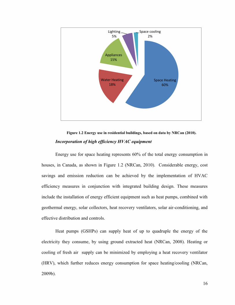
Figure 1.2 Energy use in residential buildings, based on data by NRCan (2010).
Incorporation of high efficiency HVAC equipment
Energy use for space heating represents 60% of the total energy consumption in
houses, in Canada, as shown in Figure 1.2 (NRCan, 2010). Considerable energy, cost
savings and emission reduction can be achieved by the implementation of HVAC
efficiency measures in conjunction with integrated building design. These measures
include the installation of energy efficient equipment such as heat pumps, combined with
geothermal energy, solar collectors, heat recovery ventilators, solar air-conditioning, and
effective distribution and controls.
Heat pumps (GSHPs) can supply heat of up to quadruple the energy of the
electricity they consume, by using ground extracted heat (NRCan, 2008). Heating or
cooling of fresh air supply can be minimized by employing a heat recovery ventilator
(HRV), which further reduces energy consumption for space heating/cooling (NRCan,
2009b).
Space Heating 60%
Water Heating 18%
Appliances 15%
Lighting 5%
Space cooling 2%
17
Smart control management systems enable preheating or precooling the house
before the peak hours. Preheating and precooling can be readily applied in net zero
houses through strategic exploitation of thermal mass, highly efficient building envelope
and controllable mechanical ventilation (Christian et al., 2007).
Domestic Hot Water, Lighting and Appliances
Solar thermal collectors can provide around 55% of the DHW demand for
residential applications (Kemp, 2006). A typical solar hot water system consists of a solar
collector, circulating system to transfer heat from the collector to the preheated insulated
storage water tank and a backup water heating system. Insulated storage tanks should be
used to eliminate heat losses.
Low-energy appliances can reduce electricity demand in the range of 10%-50%
(as in ENERGY STAR appliances; Pellant and Poissant, 2006).
Appliances, DHW and lighting loads for NZEH
Various sources list the energy load for major and minor appliances for household
in Canada. Major appliances include refrigeration equipment (freezer and refrigerator),
dishwasher, washing machine, clothes dryer and cooking appliances. Minor appliances
include wide range of appliances used in the kitchen and for entertainment purposes.
Armstrong et al. (2009) determined the annual consumption targets for three
typical Canadian detached households - Low, medium and high energy households. A
total energy load of 4813 kwh/y was computed for a low energy household of 141m2.
Charon (2007) determined average electricity consumption for household
appliances. The study included energy efficient and Energy Star appliances. A total
18
electricity consumption of about 1450kWh/y was computed for minor appliances and
about 2000kWh/y for major appliances.
Analysis of a Canadian NZESH (Pohgarian, 2008) assumed a total of 3 kWh /day
(about 1095 kWh/y) for minor appliances, and about 1600 kWh/y for major appliances.
This shows a significant reduction (28%) relative to the figure given by Armstrong et al
(2009), demonstrating that energy efficient appliances can significantly reduce the
electricity consumption.
Sartori et al (2010) indicated that NZESHs should limit electricity consumption
for all appliances and plug-loads to 800kWh/y or less, per occupant. Electricity
consumption for lighting, estimated as 1100 kWh/year in a typical low energy Canadian
house, should be reduced to less than 400 kWh/year. In fact this study proposes to restrict
the lighting consumption to about 3kWh/m2/y for a NZESH in mid-latitude locations.
This value of lighting consumption is based on the assumption that a ZESH is expected to
optimize daylight use.
Sartori et al (2010) recommend limiting hot water energy consumption to a daily
average of 2.75 kWh per occupant, based on the assumption of hot water usage of
50L/day/person. The 50L/person is based, first on reference numbers suggested by
various studies (e.g. EN 15316 (66.6 L/person) and the Canadian EQuilibrium Initiative
(56.25L/person)), and on the assumption that it is possible to reduce significantly the
DHW consumption, using different methods (such as using low-flow showerheads).

19
1.1.2 Active Solar Technologies
Active solar systems refer to systems that convert solar energy to usable energy
by means of solar collectors. Solar collectors include thermal collectors that can be used
for domestic hot water (DHW) and space heating, as well as photovoltaic (PV) or hybrid
photovoltaic/ thermal (PV/T) systems.
Photovoltaic systems are emerging as an important part of the trend towards
energy source diversification (Wiginton, 2010; Neuhoff, 2005; Pearce, 2002). PV
technology implementation is still limited however; constituting less than 1% of global
energy production (Wiginton, 2010). In Canada, building integrated photovoltaic systems
(BIPV) are estimated to have the potential of providing 46% of the total residential
energy needs (Pelland and Poissant, 2006). This figure is determined based on a
conservative methodology which estimates the available area of roofs and facades for
integration of grid connected PV systems, while accounting for architectural and solar
constraints (Technical Report IEA-PVPS T7-4, 2002).
Building Integrated Photovoltaic Systems
PV systems can be used as an add-on over the building envelope (building add–on
photovoltaic system (BAPV)), or integrated into the envelope system (BIPV). BAPV
requires additional mounting systems while the BIPV system is an integral part of the
building envelope construction and has therefore the potential to meet all its requirements
(such as mechanical resistance, weather protection, etc.). BIPV and BIPV/T systems,
referred to as building integrated hybrid photovoltaic/thermal systems, are assumed in
this research.

20
Introduction to PV
The electricity generated by a PV system constitutes only a fraction of the solar
radiation absorbed by the system surface, referred to as the electrical conversion
efficiency of the PV modules. The remaining energy is partly converted to heat (Poissant
and Kherani 2008).
Existing electrical efficiency of some of the commonly used PV modules such as
polycrystalline and monocrystalline silicon ranges currently between 20% and 25% while
the electrical efficiency of amorphous silicon (a-Si) PV reaches 10% ( Green et al,
2011). Thin film silicon modules are being developed with increasing efficiency,
currently reaching some 16%. The electrical conversion efficiency is measured under
standard conditions (solar irradiation of 1000 W/m2 and cell temperature of 25°C) (Green
et al, 2011).
The performance of a PV system depends mainly on the tilt angle and azimuth of
the collectors, local climatic conditions, the collector efficiency, and the operating
temperature of the cells. During the winter months, the insolation can be maximized by
using a surface tilt angle that exceeds the latitude of the location by 10-15º. In summer an
inclination of 10–15º less than the site latitude maximizes the insolation (Duffie and
Beckman, 1991). The PV system is commonly mounted at an angle equal to the latitude
of the location, to reach a balance between winter and summer production (Kemp, 2006).
In locations where snow accumulation is an issue, the tilt angle should be selected to take
into account this factor.
The orientation of the PV panels affects both the electricity generation and the
time of peak generation. PV system orientation can be selected to better match the grid

21
peak load (Holbert, 2009). This can affect the annual return value of the produced
electricity, especially in locations where electricity value changes with time of use
(Borenstein, 2008).
Hybrid photovoltaic /thermal systems (PV/T)
Hybrid photovoltaic/thermal systems (PV/T) combine PV modules and heat
extraction devices to produce simultaneously power and heat (Tripanagnostopoulos,
2001). Heat extraction from the PV rear surface is usually achieved using the circulation
of a fluid (air or water) with low inlet temperature. The extraction of thermal energy
serves two main functions. It is exploited for space heating and solar hot water
applications, and it serves for cooling the PV modules, thus increasing the total energy
output of the system (Charron and Athienitis, 2006).
The total electrical and thermal energy output of the PV/T systems depends on
several factors including solar energy input, ambient temperature, wind speed, and heat
extraction mode. For locations with large space heating requirements, air based PV/T
systems can be particularly advantageous and cost effective (Tripanagnostopoulos et al,
2001).
Integration of PV in the Building Envelope
Integration of PV panels into the building design as BIPV is gaining much
attention. For instance, the International Agency of Energy (IEA) has launched IEA Task
41- Solar Energy and Architecture (IEA Task 41, 2009) to investigate the architectural
integration of solar collectors in buildings. The mission of this task includes the
identification of barriers for integration of solar collectors, providing guidelines for

22
integration and identification of successful examples of architectural integration of PV
systems and solar thermal collectors, around the world.
Advantages of building-integrated photovoltaic systems include architectural,
technical and financial aspects. Some of these advantages are summarized in the
following:
The electricity is produced on site, thus reducing the cost and impact of transport
and distribution (Mueller, 2005).
Elimination of the structural framework required to support free standing solar
collectors. This can help in offsetting the cost associated with the additional
support structure, as well as the cost of multiple roof penetrations for the
supports (Pearsall and Hill, 2001).
BIPV panels are designed to substitute the external skin of the building envelope
(i.e. PV as a cladding), or to substitute the whole technological sandwich (e.g.
semitransparent glass-glass modules as skylights), and therefore it can
counterbalance the price of the building materials and systems it replaces
(Pearsall and Hill, 2001).
No additional land area is required, since the building surfaces are used to mount
the system, thus allowing its application in dense urban areas (Pearsall and Hill,
2001).
PV systems have generally a long life span and require no maintenance
(Mueller, 2005).

23
PV systems offer a multitude of architectural design solutions, ranging from
urban planning scale to specific building components (e.g. shading devices,
spandrels, etc.) (Kaan and Reijenga, 2004).
BIPV systems have few disadvantages as compared to add on PV modules
(BAPV), the most significant is its higher cost (Pearsall and Hill, 2001). This cost
however is continuously decreasing (see below). The application of BIPV systems is
more suitable for new buildings than to retrofitted buildings.
Aspects of Integration
A multidisciplinary approach is required to achieve a successful integration of
BIPV systems. Several aspects should be considered including architectural, functional
and technical aspects. A summary of some of these considerations is presented below.
Architectural/ aesthetic integration: Several ways of architectural integration have
been identified (IEA Task 7, 2000). These include neutral integration, where the
system does not contribute to the appearance of the building, or prominent
integration, where the BIPV system is distinguished from the total building
design. An important criterion of a good architectural integration is the overall
coordination with the design of the building.
Functional integration: Solar collectors can be engineered to serve multiple
functions. Examples include passive solar design elements (awnings, light
shelves, etc., see below) and as roof and façade cladding materials (Keoleian and
Lewis, 2003).

24
Technical integration: This refers to the integration with the building systems,
such as the structural, mechanical and electrical systems. For instance, the
integration of the BIPV/T system with the building HVAC system can contribute
to energy savings by preheating fresh air intake. Electrical integration includes
voltage and current requirements, wiring methods, in addition to the utility
integration.
Building envelope incorporating BIPV systems must be designed to resist
water infiltration that may penetrate the framework into the BIPV interlayers, must
provide a weather seal and control thermal transfer. In addition, the BIPV systems
must be able to withstand the stresses that a building envelope is subjected to,
including thermal expansion.
Methods of Integration of PV in the Building Envelope
BIPV systems can be designed to cover a part or total area of roofs or facades, or
as added components on these surfaces.
Roofs:
There is an intense interest to integrate PV systems in the roofs especially in
residential or low rise buildings, since it can provide an ideal exposure to solar
radiation. BIPV products are becoming commercially available, that can
substitute some types of traditional roof claddings such as tiles, shingles and
slates (Fig. 1.3). These BIPV products are developed to match existing building
products and are therefore compatible with their mounting systems.

25
Prefabricated roofing systems (insulated panels) with integrated thin film
laminates (Fig. 1.4) are starting to penetrate the market as well. These PV
“sandwiches” constitute complete PV systems that comprise PV modules with
mounting and interface components. Such products often include dummy
elements to facilitate the aesthetical integration.
(a) (b)
( (d)
Figure 1.3, (a) Shingle PV, (b) PV Tiles (c) PV slates (Uni-Solar, 2011), (d) PV laminates
(Solar Power Panels, 2011).
(a) (b)
Figure 1.4, (a) Solar sandwich (Best Solar Energy, 2011), b) solar roof system (Systaic, 2011).

26
Semi-transparent PV systems can be used in skylights, where semi-
transparent crystalline or translucent thin film panels are most commonly
employed.
Façades:
A PV system can substitute the external layer of façades, as a cladding
component, or it can substitute the whole façade system (e.g. curtain walls –
opaque or translucent). In the case of PV as external cladding, the back is usually
ventilated, to avoid overheating of the panels and lowering the electrical
efficiency of the system. The heated air can be employed for space or water
heating. Different curtain wall structures can offer a multitude of architectural
appearances (Fig. 1.5).
(a) (b)
Figure 1.5, (a) GreenPix Media Wall, (Beijing, China (© Simone Giostra & Partners/Arup);
(b) Solar decathlon (façade from Onyx).
External Components:
PV panels can be employed as external components to serve various functions
such as shading devices, spandrels or balcony parapets. Figure 1.6 shows examples of
BIPV systems as window shutters and awnings.

27
(a) (b)
Figure 1.6, (a) PV panels as window shutters, (Colt international, 2011); (b) Solar awnings,
(Solar Awning inbalance-energy.co.uk).
Cost of PV Systems
The average price of PV is currently around 3$ per Watt peak (Wp) (Solarbuzz,
2011). Due to market extension and the increased production volume, prices are dropping
steadily (Fig.1.7). A feasible long term cost potential of PV module that ranges between
0.3 USD/Wp and 0.6USD/Wp is estimated (Curtright, et al. 2008; Pietzcker et al., 2009).
At this price, it could be economical to integrate PV systems not only on the equatorial
facing roofs and /or facades, but also on west and east sides of the building. Figure 1.2
depicts the cost of PV systems over the last 30 to 40 years.
Cumulative PV (MW)
PV Price [$2010/W]

28
Figure 1.7, PV cost index per cumulative production (Breyer and Gerlach, 2010).
PV price depends directly on the Watt - peak capacity of a panel. Watt Peak is
defined as the power a module can deliver under standard test conditions (solar
irradiation of 1000 W/m2, and temperature of cells at 25°C). Consequently, it is possible,
given a predetermined budget, to cover different surface areas of roofs or façades by
using different available technologies. For instance the decision maker can opt for a small
PV area (used as overhangs or other similar functions), where the PV system has high
electrical efficiency and high price, or to a large surface area, with low electrical
efficiency and low cost.
The financial return of PV electricity generation can be broken into two main
parts: 1) Initial immediate return through subsidies (see below), and 2) Energy saving and
selling to the utility (Holbert, 2009). Immediate return on the cost of PV systems is
usually obtained through utility and governmental incentives that provide investment
subsidies. In these cases the authorities refund part of the cost of installation of the
system, as well as offering the owners (in commercial and residential projects) a premium
price for all the renewable power produced at their site.
Moreover, selling the excess electricity to the grid can reduce the payback period
for the original cost of PV systems. Currently, there are several incentives that buy the
electricity at a price that can significantly reduce the payback period. These incentives
include feed-in tariffs (FIT), and time of use (TOU). These are summarized below.
Feed-in tariffs/net metering: the electricity utility buys PV electricity from the
producer under a multiyear contract at a guaranteed rate. The solar buyback rate
can be large enough to cover the cost for the remaining electricity need at the

29
going residential rate. Currently in Canada, only Ontario offers significant
incentive through the feed-in tariff program for renewable energy employed to
encourage installation of PV systems for renewable energy generation (CMHC,
2010).
Time of use plans: According to this plan, the cost of electricity varies as a
function of time and day (due to demand variations). When demand is high the
electricity price is high and vice versa. In locations where prices of electricity
vary with TOU, annual return on energy produced may be a more important
object than the amount of energy produced. Favorable timing of the PV electricity
generation can increase its value by up to 20%. This premium value of PV can be
improved by 30-50% when price responsive demand and peaking prices strategies
are used (Borenstein, 2008).
1.2. Energy Performance of Buildings and Neighborhoods
Energy use in a community is not restricted to building operations, but
encompasses industry, vehicles, and infrastructure. Carlisle (2009) defines a zero-energy
community as a community where the total energy needs for vehicles, thermal, and
electrical energy within the community, is met by renewable energy. This research is
however restricted to two-storey dwellings within small scale residential neighborhoods.
This research can be considered as the first stage in the process of studying net zero
energy neighborhoods.

30
1.2.1. Energy and Building Shapes
Building shape plays a major role in governing energy consumption and can
provide advantages in capturing solar energy (Ouarghi and Krarti, 2006). The following
section presents a survey of the main literature addressing building shape effects on solar
capture and energy performance.
Effects of Building Shapes on Solar Potential and Energy Consumption
Studies that approach methodically the effect of building shape on its potential to
capture and utilize solar energy are rather scarce. The existing examples in literature
focus primarily on the dimensional proportions of rectangular buildings, on orientation of
the building, or on vertical self-shading of the building (e.g. due to overhangs) (Olgyay,
1963; Knowels, 1981 & 2003; Capeluto, 2001). Very few studies deal with buildings of
non-rectangular floor plans and their effect on total insolation. For instance Ling et al.
(2007) studied the effect of high-rise buildings of two convex geometric shapes –
rectangular and oval, with different relative dimensions on the total insolation. The goal
of the study is to identify the optimum shape in minimizing total solar insolation in low
latitude regions.
Research into the effects of building shape on energy performance, as distinct
from solar potential, has been quite extensive. Two main approaches are employed in
these investigations. The first approach consists of studying the effect of changing a few
geometrical parameters and building envelope characteristics on the energy performance
of a pre-defined shape. The second approach applies optimization methods to generate
energy efficient building shapes.

31
Shape and Envelope Effects
Rectangular Shape
The first approach ‒ evaluating the effect of shape on energy performance ‒ is
mostly limited to the study of variations of rectangular shape. These variations consist
mainly of studying the effect of compactness of the building or relative dimensions of the
equatorial façade to the perpendicular façade (see aspect ratio below). Simple numeric
indicators that focus on building's geometric compactness are usually applied (Heindl and
Grilli, 1991; Mahdavi and Gurtekin, 2002). Compactness is usually represented by what
is termed a shape coefficient, defined as the ratio of the overall building envelop surface
to the inner volume of the building. For instance, Depecker et al. (2001) established a
linear dependence between compactness and heating demand based on 14 buildings
derived from the same basic rectangular module.
A significant parameter in the design of the dimensions of rectangular solar
buildings is the aspect ratio, defined as the ratio of the equatorial-facing façade width to
that of the lateral façade. The aspect ratio is emphasized in various studies as an
important factor in energy efficient building designs, under different climate conditions.
In cold climate, the optimal aspect ratio for a rectangular shape solar house design ranges
from 1.3 to 1.5 (Chiras, 2002; Charron and Athienitis, 2006).
Understanding the limitations of the compactness factor as representative of
building shape, a number of studies venture beyond the rectangular shape. For instance,
Pessenlehner and Mahdavi (2003) analyzed the influence of additional parameters
including the overall geometry of the building, the glazing area and the orientation.

32
Multiple shapes were generated, employing a modular geometry system based on
elementary cube. Their research demonstrates that compactness and the portion of
glazing of the building envelope significantly impact the thermal performance of various
residential building shapes. They concluded that simple geometrical indicators such as
the shape coefficient (presented above) are incapable of capturing non-rectangular
geometries, and therefore of predicting phenomena such as the risk of overheating of
buildings.
Non-rectangular shapes
Ouarghi and Krarti (2006) correlated the annual energy consumption of office
buildings with their relative compactness. Two building shapes studied in this
investigation are rectangular and L shapes. Al-Anzi et al. (2009) further developed the
method introduced by Ouraghi et al (2006). Applying linear regression, they developed a
correlation model to predict the impact of building shape of office buildings on energy
efficiency for various window areas and glazing types. Several high rise building shapes
were investigated in their study, including rectangular shape, L-shape, T-shape, Cross-
shape, H-shape, and U-shape. To obtain various dimensions of the studied shape
configurations, they changed the bounding rectangles of each shape while preserving the
same floor area. The main results of their study indicate that three factors have major
effect on total building energy consumption - relative compactness, window-to-wall ratio,
and glazing type,.

33
Shape Optimization
In the second approach ‒ shape optimization for energy performance ‒ several
research projects employ multiple optimization criteria. In most of these investigations
simple convex geometrical forms such as rectangular or polygonal shapes are employed
to represent the building. Some investigations consider several geometric variables in
their optimizations, like wall lengths, building height, walls angles, window sizes and the
thermal resistance of external walls (Adamski and Marks 1993, Jedrzejuk and Marks
1994). The optimization of the volume of a building in arbitrary and polygonal plan is
also considered in a few studies (Marks, 1997; Jedrzeju and Marks, 2002; and Adamski,
2007). However, the issue of design, including functional aspects, is not raised in any of
these studies.
More recently, Yi and Malkawi (2009) developed an optimization method to
generate shapes based on their thermal performance. The method enables generating
sophisticated shapes with multi-surface envelopes and irregular plans. EnergyPlus
program was employed as the engine for the simulations. Results of simulations
conducted in a specific location demonstrate that during summer, the optimized form
should have more shaded surface areas resulting in concave building enclosure especially
on its south, east and west surfaces. These concave surfaces should not be too deep, so as
to avoid shade during the winter period.
Although this is an interesting approach, the functionality and cost of the design
are not addressed. Functionality can be a major issue especially for dwellings, where the
utilization of spaces and their partitioning are of primary importance.
34
1.2.2. Effects of Urban Design
Neighborhood design is governed by three main factors: land use, density of
development and arrangement of streets. These parameters are usually prescribed for a
given site. Solar neighborhood designed for exploitation of useful solar radiation for
heating, daylight and electricity generation, require consideration of additional
parameters, such as building geometry, roof shapes, the arrangement of housing units
along streets and the configuration to match the required density (e.g. attached units,
rows). These design parameters, which have substantial impact on passive solar gain,
daylighitng and the feasibility and performance of photovoltaic systems, can be
manipulated to achieve net zero energy neighborhood. High density development is
associated with low energy use per capita (Steemerrs, 2003). On the other hand, high
density may reduce solar access and consequently solar energy utilization potential. Solar
access and solar radiation distribution should be considered from the earliest planning
stages to ensure that the majority of buildings on a site, in the northern hemisphere, are
oriented between south east and south west in order to have good solar access (Erley and
Jaffe, 1979). Size and shape of a site, as well as the layout of streets within this site can
influence orientation of buildings and therefore their accessibility to solar radiations
(Knowles, 1981).
Solar Potential in Urban Areas
Solar radiation in the urban context has been extensively studied over the past few
decades. Techniques have been developed for building specifications to minimize mutual
shading by buildings and to determine insolation or shading in a given urban area. For

35
instance, Arumi (1979) established a model to define the maximum allowed height of a
building to avoid overshadowing its surrounding.
Knowles (1981) suggested a method termed solar envelope, to assure solar access
to each residence unit in a community. The solar envelope consists of an imaginary
boundary based on the sun’s relative motion. Buildings contained within this envelop do
not jeopardize the solar rights of their neighboring buildings during critical periods of
solar access.
Compagnon (2004) proposed a methodology for estimating the amount of solar
energy available to a building of arbitrary shape, taking into account obstructions due to
the surrounding landscape and associated reflections. Montavon et al. (2004) and
Scartezzini et al. (2002) developed a procedure to produce histograms of irradiation as a
function of built portion in a specific urban area.
Several studies have focused on the distribution of solar radiation on different
surfaces in a built environment (e.g. Ouarghi and Krarti, 2006; Stasinopoulos, 2002;
Leveratto, 2002), as well as the availability of solar energy and its optimization, at the
urban scale.
Mardaljevic and Rylatt (2000) computed irradiation in complex urban
environments using the ray tracing program RADIANCE. RADIANCE has also been
applied to study the periodic (annual or winter) solar distribution as a function of built
area (Compagnon, 2004; Mardaljevic, and Rylatt, 2000; and Cheng et al., 2006).
Ghosh and Vale (2006) determined the solar energy potential for a New Zealand
neighborhood by using geographic information system (GIS) to calculate the roof area

36
suitable for solar thermal and solar PV (Ghosh, et al., 2006). GIS system is usually
employed for mapping and analysis of geographic data.
Energy Consumption in Urban Areas
Extensive research has been conducted to estimate the energy consumption of
urban areas as large as whole cities. Various methods are developed to determine the
effect of urban form on energy demand of buildings.
Ratti et al. (2005) used Digital Elevation Models (DEM) ‒ a 3-D representation of
a terrain surface created from its elevation data, including building elevations ‒ to
determine the effects of urban texture on energy consumption. The DEM method is
employed to refine the “solar envelope” method (Knowels, 1981, see above) so it reflects
accurately the solar radiation over a large urban area and simplifies the calculations of
this solar envelope.
Christensen et al (2008) propose a computerized Subdivision Energy Analysis
Tool (SEAT), which allows an interactive design of street layouts while receiving
feedback on energy impact.
The urban energy consumption simulator CitySim is under development, based on
multiple physical models. CitySim can compute an estimation of the on-site energy use
for heating, cooling and lighting (Perez et al. 2011).
Other investigations have focused on establishing approaches to minimize energy
use in various built environments. For instance, Kampf et al (2010) developed a
methodology to reduce energy demand of buildings in an urban area employing
multiobjective evolutionary algorithm to maximize incident solar irradiation whilst

37
accounting for thermal losses. The shapes of three commonly used urban forms are
optimized in this study – terrace flat roofs, slab sloped roofs and terrace courts.
Cheng et al. (2006) conducted a parametric study of 18 different models,
representing various combinations of built form and density. The trial and error method
they employed was unlikely to identify an optimal geometric form in terms of
maximizing the solar irradiation potential, given the small number of cases tested.
Pol et al. (2011) summarized the main findings of the impact of urban
morphology on energy needs in the built environment. The study shows that there is no
common basis allowing for a generalization of the knowledge available.
Solar Parameters of Urban Design (Neighborhoods)
Two approaches are adopted to analyze energy performance of urban areas. The
first approach uses models representative of real urban design morphologies. These cases
are usually limited in their ability to generalize the findings, unless the studied
morphologies can represent ubiquitous prototypes.
The second approach is based on simplified urban morphological archetypes
which can be easily parameterized, both for performing sensitivity analyses and for urban
morphology optimization. The major problem of this approach is the risk of not
representing realistic urban design forms. The most frequently assessed archetypes are
pavilions (Morello and Ratti, 2009; Morello et al. 2009), including shape variations for
high-rise buildings (Leung and Steemers, 2009), courtyard configurations (Kämpf and
Robinson, 2010), row houses (Jabareen, 2006) and urban street canyons (Ali-Toudert,
2009).
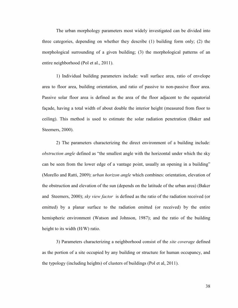
38
The urban morphology parameters most widely investigated can be divided into
three categories, depending on whether they describe (1) building form only; (2) the
morphological surrounding of a given building; (3) the morphological patterns of an
entire neighborhood (Pol et al., 2011).
1) Individual building parameters include: wall surface area, ratio of envelope
area to floor area, building orientation, and ratio of passive to non-passive floor area.
Passive solar floor area is defined as the area of the floor adjacent to the equatorial
façade, having a total width of about double the interior height (measured from floor to
ceiling). This method is used to estimate the solar radiation penetration (Baker and
Steemers, 2000).
2) The parameters characterizing the direct environment of a building include:
obstruction angle defined as “the smallest angle with the horizontal under which the sky
can be seen from the lower edge of a vantage point, usually an opening in a building”
(Morello and Ratti, 2009); urban horizon angle which combines: orientation, elevation of
the obstruction and elevation of the sun (depends on the latitude of the urban area) (Baker
and Steemers, 2000); sky view factor is defined as the ratio of the radiation received (or
emitted) by a planar surface to the radiation emitted (or received) by the entire
hemispheric environment (Watson and Johnson, 1987); and the ratio of the building
height to its width (H/W) ratio.
3) Parameters characterizing a neighborhood consist of the site coverage defined
as the portion of a site occupied by any building or structure for human occupancy, and
the typology (including heights) of clusters of buildings (Pol et al, 2011).

39
1.2.3. Case studies
Under current market conditions financial incentives on the part of governments
and/or the utility companies are essential to make the implementation of solar technology
viable at the urban scale. Most urban-scale PV projects to date have obtained some level
of capital funding subsidy.
A growing number of projects related to application of BIPV systems at an urban
scale are reported in different locations in the world. Examples of these applications are
presented by the International Energy Agency - IEA PVPS Task 10 (IEA-PVPS-Task
10). Some of the most advanced countries in design and application of solar urban
projects include Germany, the Netherlands, Japan and the United States. In general, these
projects try to maximize total electricity production. A few examples of urban solar
projects are presented below, accompanied by a discussion of some of the main
characteristics related to form optimization, urban planning issues and technologies
employed (PV, combined heat and power etc.). None of the reported projects, however,
includes methodic approach to the design of solar energy efficient communities/
neighborhoods, aiming at achieving net zero energy status.
Clarum Homes ‒ Vista Montana (USA)
Vista Montana is one of many zero energy home developments by the Clarum
Homes Development Company, in the United States (Clarum Houses, 2003). A PV
system is installed on the roof of each housing unit (Fig. 1.8). The PV system electricity
generation together with energy efficiency features, result in reduction of overall net
energy demand by some 90%, compared to conventional houses. The layout of the
development ensures an economical land use.

40
Figure 1.8, Aerial view of the Clarum houses in the USA(Clarum houses, 2003).
Solarsiedlung am Schlierberg, Freiburg, (Germany)
Solarsiedlung am Schlierberg is a mixed-function development that comprises
residential and commercial buildings. Large areas of photovoltaic modules are installed
in a plane above the south facing roofs of the various buildings. Asymmetrical gable
roofs and shed roofs are adopted to increase the area of the roofs for PV installation (Fig.
1.9d) (Hagemann, 2007). Both roof styles have large overhangs on the south face and
therefore provide shading on these facades in summer, while further increasing the roof
surface for PV integration. An air-gap of 16 cm is designed between the roof and the PV
plane. Although structurally and functionally the PV array and roofing systems are
separate, the two systems form a well-integrated feature of the roof complex.
The energy generation is complemented by energy efficiency measures.

41
Figure 1.9, Solarsiedlung am Schlierberg, Freiburg (Breisgau) (a) view of muli-story
buildings and terrace houses, of Mixed-function development, (b) plan view, (c) detail of the
overhang of a terrace house, (d) terrace house (Hagemann, 2007).
The Nieuwland (Netherland)
The Nieuwland 1 MW PV project involves the implementation of PV systems on
a large scale. The solar electricity contributes about 54% of total energy consumption.
The urban planning consisted originally of east-west oriented houses. This
original planning was subsequently modified so as to optimize the development for solar
radiation access. This allowed the development to achieve a target level of 20 m2 PV per
household. The land was parceled to maximize the roof surface areas that are suitable for
PV integration, to reach the level of 1 MWpeak.
The houses were developed using recognized concepts for technical integration of
PV panels, taking into consideration the orientation, inclination and ventilation. The
resulting architectural design shows a great variety of building integrated PV systems,
(
a)
(
d)
(
c)
(
b)
(c) (d)
(a) (b)

42
oriented between SE and SW, with tilt angles ranging between 20° and 90° (Figs. 1.10 a-
d). Solar modules are used as roofing tiles, facade cladding and as sunshades. The water
tightness of the PV roofs was guaranteed by a watertight layer under the solar modules.
Some unforeseen issues such as shading and non-optimal orientation and tilt angle caused
5 to16% underperformance in electricity generation (SECURE: Niewland solar energy
project).
The utility company owns the PV systems; therefore the electricity generated is
fed directly into the public grid.
(a) (b)
(c) (d)
Figure 1.10, PV integration in Nieuwland, (a) on the roof of a parking lot; (b) in sport
complex, (c) noise wall houses, (d) Prefab PV roofs (PV UPSCALE: Nieuwland, 2008).

43
Kanokodai (Japan)
The community has 95 houses equipped with BIPV systems. To create a well-
designed appearance of the houses and a harmonized streetscape as a community
(Fig.1.11), PV roof tiles were selected for the PV systems. The houses were customized
to the inhabitants’ requirements.
The PV system received a governmental subsidy. A net-metering scheme was
applied so that excess of electricity generation is sold to the utility company, at a price
that equals the residential electric tariff (IEA PVPS-Task 10: Japan: Jo-Town
Kanokodai).
Figure 1.11 Jo-Town Kanokodai (MSK corporation, IEA PVPS-Task 10: Japan:
Jo-Town Kanokodai).

44
Table 1.1, Summary of case studies
Name and photo or
schematic
Solar
design/optimization
Energy system
(BIPV, CHP etc) and
key stats)
Energy storage
system /grid
Density and other
urban issues
USA-Clarum Homes – Vista
Montana Houses - South orientation
Energy use reduction
of 90% as compared
to conventional
houses.
BIPV system Total
PV power: >300 kW
PV power per unit:
1.2 to 2.4 kWp
Grid connected PV
system
The systems are
interconnected
and net
metered
177 single-family
homes, 80
townhouses, and 132
apartments
The development
layout is a grid
(economical land
use).
Germany- Solarsiedlung am
Schlierberg, Freiburg
(Breisgau)
South orientation
Inclination (Terrace
houses): 22 º
Gable shed roofs are
used to increase the
area of PV
integration.
An air-gap of 16 cm
between the roof and
the PV plane.
PV-System size: 445
kWp , 2 million kWh
primary energy
savings per year
Active ventilation
with heat recovery
Contribution solar
electricity in total
consumption: 54%
Grid connected PV The “Sonnenschiff”
is complete solar
development retail,
office and living two
or three stories high
while the
commercial
buildings are four to
five stories high.
The Netherland- The
Nieuwland
Orientation: between
SE and SW,
Tilt angles: ranging
between 20° and 90°.
PV total power: 1
MGWp PV
PV power per
system/house: 0,8 -
4,4 kWp
A solar/gas
combination unit,
15kW capacity each,
has been installed in
each house
Grid connected
PV.
Experiments using
ground water (12m
depth) for long
term storage
Electric heat
pumps (as part of
experimental work
on semi detached
houses)
The urban plan
optimized for solar
access, (since design
stage).
The land is parceled
to maximize the roof
surface areas that are
adequate for PV
integration (around
20m2 /roof)
Japan: Jo-Town Kanokodai Inclined roof
PV roof tiles were
selected for the PV
systems.
Total PV power: 285
kW
PV power per unit: 3
kW/house
Option of all –electric
houses
Grid connected PV
net-metering
scheme
The community has
95 houses
Customized housing
design

45
Discussion of the Case Studies
Table 1.1 provides a summary of the main features of each of the case studies. Some of
the main observations made in these cases are discussed in the following:
Urban planning for PV Integration. In many of the presented case studies, the
decision of integration of PV systems was taken at a late stage in the urban
planning process, after the site selection and sometimes after construction of the
buildings. In some projects, such as in Germany and in the Netherlands, solar
access was planned before the implementation of the large scale PV systems. In
the German case study, detailed and shading simulations were performed on the
development site, and the results were used to guide the designers. The
Nieuwland case study solar optimization was taken into account in the urban
planning phase with the land being parceled out to provide as many roof surfaces
as possible suitable for the installation of solar panels.
Optimization of the design process. A systematic approach to analyze building
shape potential was not generally conducted in the presented cases. PV systems
were installed on surfaces that present a good solar layout. Therefore building
geometry and roof designs were not specifically designed to maximize the solar
potential. For example, in Germany, the original roofs were modified and
additional separate structures were built to support the PV systems, in order to
obtain a large surface of roof at an acceptable tilt angle. In the Netherlands
different ranges of orientation and tilt of the PV systems were attempted, resulting
in some reduction in the generation potential of the systems.

46
Consumption vs. generation. Most of the projects were concerned mainly with
maximizing electricity generation. In general, there is no procedure for energy
balance between consumption and generation.
Role of government and utilities. Governments together with utility companies
played an important role in all the case studies. In some cases the utility
companies own the PV systems, such as in the Netherlands, and therefore the cost
of the PV systems was provided by these companies, while the electricity
generation was fed directly to the grid. In most of the other cases the government
paid a subsidy to install the PV systems. The excess of the electricity was in most
cases sold to the grid with a price at least equal to the tariff of use.
1.3. Tools
1.3.1. Modeling of Net-Zero Energy Solar Houses
Modeling net-zero energy solar houses (NZESH) requires a systematic approach
to predict the dynamic response of buildings and their systems and the interaction with
on-site renewable energy generation (Athienitis et al, 2010). It is recommended to
employ simulation programs at early design stages of NZSEH in order to attain the pre-
established performance goals (IEA- SHC Task 40/ECBCS Annex 52). More advanced
models may be needed in later stages to enable detailed analysis.
For the early design stage, when the shape of building is almost determined,
simulations can assist in determining basic parameters such as optimal window size,
thermal mass, PV size and its optimal location. Existing simple tools are limited in their
capability to model basic NZESH design characteristics, including daylighting, natural

47
ventilation and location of thermal mass. For instance, tools like RETScreen (RETScreen
International, 2005), can be employed to size BIPV systems; however it cannot model
complex roof shapes or predict the effect of shading on electricity production. At more
advanced stages, simulation tools that offer possibilities to combine actual climate data,
various geometries, passive solar gain, HVAC-systems, energy-generation systems,
natural ventilation, together with user behavior (occupancy, internal gains, manual
shading) are required.
A number of simulation tools, with varying capabilities, are currently available
(Hong et al., 2000; Al-Homoud, 2001; Crawley et al., 2001and 2008). Programs that are
commonly encountered in the literature and can simulate different technologies include
TRNSYS (TRNSYS, 2004; Klein et al. 1976), ESP-r (Clarke et al., 2002) and Energy
Plus (Crawley et al., 2000; Crawley, 2001).
TRNSYS is a powerful program with large capabilities in the modeling of active
solar systems, but has some weaknesses in whole building energy modeling (Beccali et
al., 2005).
ESP-r (Energy System Performance – research) is an integrated building and plant
energy simulation environment. It supports early-through-detailed design stage
applications and enables integrated performance assessments. It offers climatic data,
construction, profiles database management, and incorporates shading, solar beam
tracking, condensation analysis; air flow modelling, etc. (Clarke, 2002).
EnergyPlus has a large potential, given the fact that it is well-funded, free of
charge, and has many commercial front-ends. The user can select the method of heat
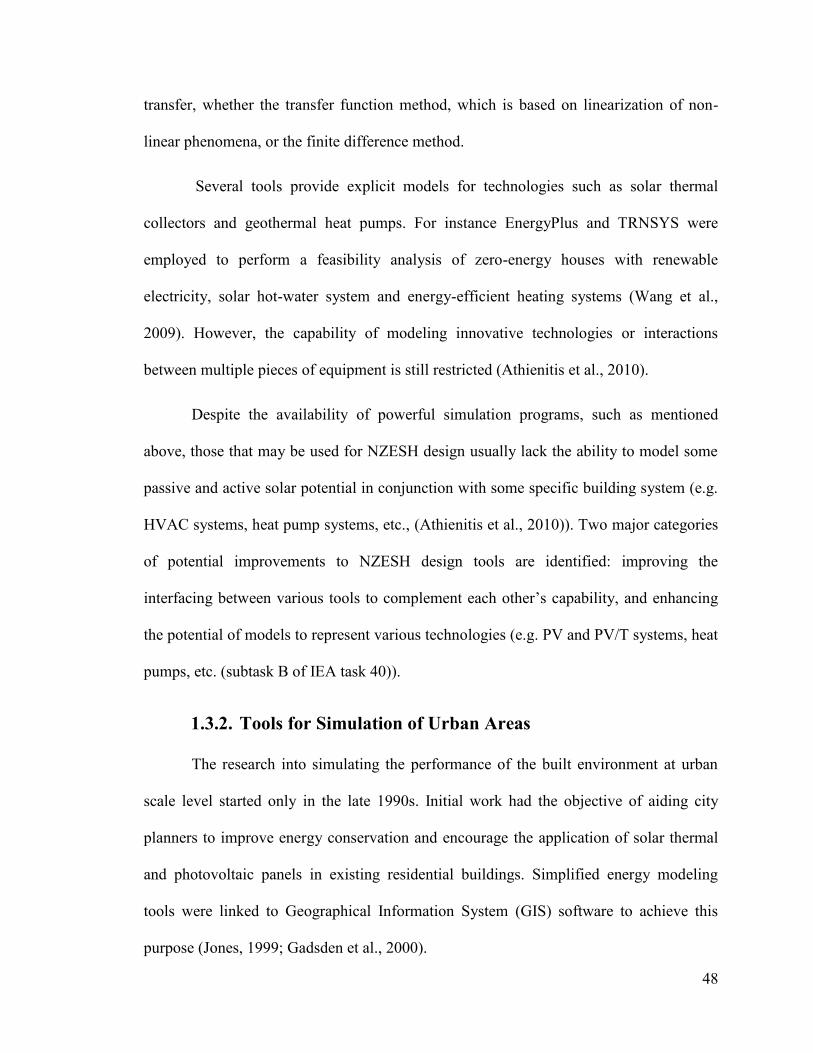
48
transfer, whether the transfer function method, which is based on linearization of non-
linear phenomena, or the finite difference method.
Several tools provide explicit models for technologies such as solar thermal
collectors and geothermal heat pumps. For instance EnergyPlus and TRNSYS were
employed to perform a feasibility analysis of zero-energy houses with renewable
electricity, solar hot-water system and energy-efficient heating systems (Wang et al.,
2009). However, the capability of modeling innovative technologies or interactions
between multiple pieces of equipment is still restricted (Athienitis et al., 2010).
Despite the availability of powerful simulation programs, such as mentioned
above, those that may be used for NZESH design usually lack the ability to model some
passive and active solar potential in conjunction with some specific building system (e.g.
HVAC systems, heat pump systems, etc., (Athienitis et al., 2010)). Two major categories
of potential improvements to NZESH design tools are identified: improving the
interfacing between various tools to complement each other’s capability, and enhancing
the potential of models to represent various technologies (e.g. PV and PV/T systems, heat
pumps, etc. (subtask B of IEA task 40)).
1.3.2. Tools for Simulation of Urban Areas
The research into simulating the performance of the built environment at urban
scale level started only in the late 1990s. Initial work had the objective of aiding city
planners to improve energy conservation and encourage the application of solar thermal
and photovoltaic panels in existing residential buildings. Simplified energy modeling
tools were linked to Geographical Information System (GIS) software to achieve this
purpose (Jones, 1999; Gadsden et al., 2000).

49
Some of the simulation programs employed for the investigation of solar access of
buildings within urban context include the ray tracing program RADIANCE, which
simulates the irradiation on façades (Compagnon, 2004; Mardaljevic and Rylatt, 2000;
Montavon et al, 2004). Those studies that employed it, however, did not consider
building energy demands.
Digital elevation models (DEMs) (see section 1.2.2) were also employed in some
cases to find the effect of urban texture on building energy consumption. These models
are based on image processing and were employed in lieu of detailed numerical
simulation of radiation exchange (Ratti et al, 2005).
Thermal building models in urban areas range from the highly simplified heat loss
calculation over the building envelope (e.g. Morello et al., 2009) to commercial or self-
developed transient building energy performance simulation tools. However, these
studies often ignore some aspects of energy needs (cooling, electricity needs for artificial
lighting, etc).
Some simplified energy models were used to establish relationships between
urban form and non-domestic energy use (Ratti et al., 2000). However, these models
were basic in their calculation of solar radiation transmission and heat flows in buildings.
Modeling of renewable energy technologies was either incomplete or absent.
A relatively new design tool - SUNtool, is developed to be employed for the early
decision stage of sustainable urban design. SUNtool contains occupant’s behavior,
daylight, heat flow, micro climate and plant & equipment models. This tool has however
a few disadvantages. At present it is restricted to some European countries, and to the

50
analysis of simple rectangular shapes. In addition, a certain expertise is required to
perform the simulations and to interpret the results (Vreenegoor et al, 2008).
An additional tool – CitySim, is still under development. This tool can estimate
on-site energy consumption for heating, cooling and lighting. To accomplish this
analysis, the tool needs complete physical description of the buildings in the form of an
Excel input file (Perez et al, 2011).

51
Chapter II: Design and Methodology
of the investigation
This Chapter summarizes the framework of the research, its objectives and the
methodology employed at each stage. The investigation of the effects of design
parameters on energy performance of dwellings and neighborhoods consists of three
main stages – 1) Effects of shape of individual housing units; 2) Neighborhood patterns
3) Roof design. At each stage the object of the investigation (residential units,
neighborhoods, and roofs) is first designed with different values of the design parameters,
followed by performing simulations and analyzing the results to assess the effects and
their significance. The employed simulation tools and modeling procedures are
introduced as well.
2.1. Outline of the Investigation
2.1.1 Background
Designing the shape of a building to optimize solar capture is an essential step in
achieving net zero energy status. In the design of a neighborhood, ensuring that the
majority of buildings have good solar access is a major objective. Poor solar access not
only reduces the efficiency of solar collectors, but also restricts the implementation of
passive solar design strategies for space heating, daylighting and solar water heating.
In general, key parameters of building geometry and urban patterns affecting solar
availability and utilization are not well defined. Moreover, existing guidelines do not

52
provide quantitative data on the effects of design parameters on energy performance –
energy consumption for heating/cooling and solar energy potential. Solar potential refers
to the potential of building and neighbourhoods to capture and utilize solar radiation.
Solar potential includes radiation incident on near equatorial-facing facades and
transmitted by the fenestrations of these façades, total solar heat gain by the windows,
and the energy generation potential by building-integrated photovoltaic and/or
photovoltaic/thermal system (BIPV/T), integrated in the near equatorial facing roof
surfaces of these units.
The successful design of energy efficient dwellings and neighborhoods that aspire
to achieve net zero energy status, while maintaining quality of life, needs the
understanding and collaboration between architects and engineers. This work attempts to
interface between engineering and architecture by providing a holistic approach to the
design of solar optimized neighborhood.
Specific issues in the design of dwellings and neighborhoods for optimized solar
potential are listed below.
1) Dwelling shape:
Existing guidelines for the design of passive solar energy efficient houses are
limited mostly to rectangular shapes. Rectangular shape is generally considered

53
as the optimal building shape for passive solar design and the most energy
efficient (Chiras, 2002). However, under certain design conditions in urban
context, this shape may not be optimal. For instance, rectangular plan does not
allow uniform penetration of daylight, especially to the north part, which is
usually, kept window free in energy efficient houses. In addition, it should be
born in mind that shape design is governed by many constraints other than
energy efficiency, such as functional demands and quality of life of inhabitants.
For these reasons it is important to explore the penalties, as well as the benefits
associated with plan layouts other than rectangular, and with different roof forms.
Integrated solar design approach that applies passive solar design principles
together with the architectural integration of solar technologies, should be
implemented at early design stages. Dwellings should be designed to provide
optimized façade potential for solar capture, that can be utilized passively in
daylighting and heating, in conjunction with optimized roof shapes for increased
thermal/electrical generation.
2) Neighborhoods:
Despite the interest in the effect of urban development on the availability and
utilization of solar energy, there is still no systematic approach for passive solar
design on the level of neighborhoods/urban areas. Such approach should define
the main parameters that affect the solar potential of the neighborhood, ranging
from the building level to the neighborhood level, and present a methodology of
application of such parameters in the design process. This integrated approach
should encompass passive solar design of buildings, roof shape for integration of

54
solar technologies, and finally the placement of units on a site and with respect to
each other.
Most of the existing studies explore existing urban areas, to study their energy
consumption and/or their availability for solar access. No study addresses the
design methodology of new residential neighborhoods/ communities for
increased solar potential. This is an important issue, especially in Canada, where
new neighborhoods and communities are continuously planned and built.
2.1.2. Objectives and Scope
Objectives
The main objectives of this research are summarized as follows:
Identifying key design parameters of housing units’ shapes and neighbourhood
patterns to increase their solar potential.
Quantifying the effect of these design parameters on a set of energy performance
criteria such as solar potential of dwellings and neighborhoods and their energy
demand/consumption for heating and cooling.
Based on results of the parametric study, developing design methodology of
houses and neighbourhoods for improved solar performance aimed at optimising
energy generation/consumption balance, subject to multidisciplinary design
constraints.
The first two objectives of this research enable an in-depth understanding of the
effects of design parameters on performance. This understanding can form a basis for
future development of advanced design tools for net-zero energy neighborhoods.
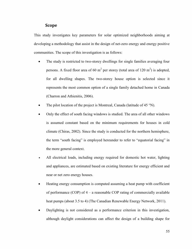
55
Scope
This study investigates key parameters for solar optimized neighborhoods aiming at
developing a methodology that assist in the design of net-zero energy and energy positive
communities. The scope of this investigation is as follows:
The study is restricted to two-storey dwellings for single families averaging four
persons. A fixed floor area of 60 m2 per storey (total area of 120 m
2) is adopted,
for all dwelling shapes. The two-storey house option is selected since it
represents the most common option of a single family detached home in Canada
(Charron and Athienitis, 2006).
The pilot location of the project is Montreal, Canada (latitude of 45 °N).
Only the effect of south facing windows is studied. The area of all other windows
is assumed constant based on the minimum requirements for houses in cold
climate (Chiras, 2002). Since the study is conducted for the northern hemisphere,
the term “south facing” is employed hereunder to refer to “equatorial facing” in
the more general context.
All electrical loads, including energy required for domestic hot water, lighting
and appliances, are estimated based on existing literature for energy efficient and
near or net zero energy houses.
Heating energy consumption is computed assuming a heat pump with coefficient
of performance (COP) of 4 – a reasonable COP rating of commercially available
heat pumps (about 3.5 to 4) (The Canadian Renewable Energy Network, 2011).
Daylighting is not considered as a performance criterion in this investigation,
although daylight considerations can affect the design of a building shape for

56
increased potential of solar utilization. Daylighting is, nevertheless, taken into
account in the design of the interior space (e.g. the location of living area, the
depth of building when it is possible and the height of the ceiling ‒ Chapter III).
Photovoltaic panels are assumed to cover the total south/near-south facing area of
roofs. Covering a complete roof surface with a BIPV system has an advantage of
forming an outer layer which acts as the weather barrier in addition to producing
useful heat and electricity.
Neighborhood characteristics, such as street widths and minimum distances
between units are based on various sources in the literature (see below and
Chapter IV for details).
Selection of parameters is based on their anticipated effect on solar potential and
energy efficiency of buildings and neighborhoods, as indicated by the pertinent
literature (Chapter I).
2.2 Methodology
This section outlines the design principles and the selection of design parameters
for the three stages of the investigation.
Shape parameters in this research are mostly selected for their effect on shading,
especially non-convex shapes. These parameters are detailed below. In addition to shape
parameters, roofs are affected by tilt and orientation angles, which govern the BIPV and
BIPV/T potential for electrical and thermal energy generation.
On the level of neighborhood, the literature emphasizes the role of road layout
and density on solar access and energy performance. For instance, site layout and roads

57
influence the position of buildings and their orientation. Density is known for its
influence on solar access, as well as on energy demand. However, these two parameters
have not been systematically investigated, separately or/and in combination, nor is their
interaction with building shape.
Details of values of the design parameters and results of the analysis of their
effects on energy performance are provided in the relevant chapters: Chapter III ‒ shape
study, Chapter IV – neighborhood study and Chapter V – roof study.
2.2.1 Shape Study
This stage, which is presented in Chapter III, investigates the effects of housing
units’ shapes on their energy performance (in terms of electricity generation and
demand/consumption). Details of the simulation procedure employed in the analysis are
given in section 2.3.
Plan Shape
The first step in the shape investigation is the design of various plan layouts of
dwellings, focusing on south façades and the position of windows in these façades. This
is followed by roof design of each shape and the integrated photovoltaic portion of the
roof. The selected configurations are then subjected to simulations to determine the solar
potential and energy demand for heating and cooling of each shape. The plan layouts
designed at this stage are divided into two main categories, convex and non-convex.

58
Convex layouts include rectangle, square and trapezoid. Non- convex layouts are
inherently self-shading. They consist of two or more wings that at certain orientations
relative to solar position may mutually shade. Non-convex shapes considered in this
investigation include: L, U, H and T shapes (Fig. 2.1).
Dwellings are designed as two-storey single family units. The two-storey option is
adopted in this study as representing one of the most common options of a single family
detached home in Canada (Charron and Athienitis, 2006). This option requires less land
compared to a single-storey house (Athienitis, 2007). The design of units incorporates
energy efficiency measures and some of the basic principles of passive solar design.
Variations of some parameters governing certain shapes such as rectangular and L
shapes are explored, to identify design possibilities that enhance solar radiation capture
potential on near-south facing roofs and façades. The effect of these parameters on
heating and cooling load/consumption is also determined.
Design parameters of rectangular shape include orientation and the aspect ratio ‒
AR (W/L in Fig. 2.2). Design parameters of non-convex shapes include the ratio of
shading to shaded façade lengths, termed depth ratio ‒ DR (a/b in Figure 2.2) and
variations of the angles between the wings. Figure 2.2 displays some of the shapes
studied, and the dimensions governing their design. The detailed presentation of all
shapes (30 different shapes), is provided in Chapter III.
Rectangle Trapezoid L T U
Convex shapes Non-convex shapes
H
Figure 2.1, Basic shapes.

59
Figure 2.2, Shape parameters.
Roof Geometry
A simple roof shape is considered for this stage of the research. The effects of
roof shape variations are investigated in the third stage. The adopted basic roof is a hip
roof with 45 ° tilt and side angles, as shown in Figure 2.3 for the rectangular plan layout.
Figure 2.4 shows the application of this roof shape to the non-convex shapes. The shape
denoted obtuse angle is a variation of L shape with a large angle between the wings (see
neighborhood design below).
Figure 2.3, Hip roof of a rectangular plan layout.
Tilt angle
E
W
Side angle
S
a
b
β
W

60
Figure 2.4, Roof shapes.
2.2.2 Neighborhood Study
The main parameters investigated in this stage are housing density and site layout.
Interactions between dwellings’ shapes, their density and the site layout are also
investigated. The response variables are the solar potential of individual units and of the
neighborhood as a whole, as well as energy load/consumption for heating and cooling.
In the design of neighborhoods, the position of trees with respect to dwellings,
their heights and type may influence the shade cast on the facades and roofs of these
dwellings (Nikoofard et al, 2011). This effect however is not considered in this research.
The design methodology consists of first determining the site layout, selecting
unit shapes to conform to the site layout, and then combining the shapes in different
configurations to fit different levels of density. All configurations are subjected to
simulations, followed by a comparative analysis to assess the effect of density and of site
layout on solar potential and energy performance, relative to a reference case. The
reference neighborhood pattern for the comparative analysis is a site with detached
rectangular units, with aspect ratio of 1.3, arranged along a straight road running east-
L variant
L
Obtuse angle
Gable
end
T U H

61
west. The studied parameters are outlined below. Full details of neighborhood patterns,
simulation results and effects analysis are presented in Chapter IV.
Site Layout
Three main site layouts are studied. These layouts are based on the CMHC fused
grid (CMHC, 2011) (Fig. 2.5). The fused grid can be a good basis for the design of a new
solar neighborhood because it is designed to allow mixed use, densification, and efficient
public transportation. All these factors are beneficial for a design of a new neighborhood
in two ways: a) they have various energy implications (use for transportation, energy
consumption in building); b) they affect affordability since all the factors mentioned
above have impact on the cost of houses.
Site layout I is characterized by a straight road. The other two layouts incorporate
semi-circular roads. In site II the curved road is south facing (i.e. the center lies south of
the arc), while in site III it is north facing.
Straight road scenarios include an east-west running road (site I), acting as
reference case, and variations, where the road is rotated relative to the east-west direction
by certain angles, in both senses (±30°, ±45°, and ±60°, with + sign implying clockwise
rotation). These variations of site I aim at studying the effect of orientation of the street
on the response variables (Chapter IV).
The circular road is selected to represent an extreme case of a curved road as, for
instance, in a cul-de-sac street design. Figure 2.5 illustrates the three site layouts, where
they represent typical segments of a large residential complex.

62
Figure 2.5, Overall site designs.
The housing units are positioned with respect to the shape of the roads in all
configurations of neighborhoods. In site I only units on the north side of the road are
considered. The shapes of units on the south side are assumed to be a mirror image of the
units on the north side. However, the main solar façade remains the south façade, which
is facing away from the road. This has architectural implications regarding the interior
design and the fenestration allocated on different facades. These architectural
implications may give some advantage to non-convex shapes, such as L and its variants,
where the wing facing the road may remain essentially unchanged. Detailed presentation
of the site layouts is provided in Chapter IV.
Density and Shapes
The main effect of increasing density of housing units is mutual shading by units
and their wings (of non-convex shapes) and reduction in the effective surface area for
insolation. Two density effects are analyzed. Spacing effect (s, in Fig. 2.6) is assessed by
comparing attached units in triplex, quadruplex or pentuplex configurations with
detached units. In addition, an effect, termed hereunder row effect, is assessed, whereby
the south façades of selected configurations of site I is obstructed by a row of similar
housing configurations (r in Fig. 2.6). Selected configurations of unit shapes (rectangle,
L shapes, and L variants) are studied with varying row spaces. The minimal distance
Site III
Site I
Site II
S

63
required between rows to avoid shading on the façade of the obstructed row is first
computed, and the distance is then incrementally reduced to assess its effect on energy
performance.
Figure 2.6, Illustration of the density parameters.
Representative shapes of dwelling units, analyzed in the previous stage (shape
study) are adopted in the neighborhood study. Shapes found to have good performance,
such as rectangular and L shapes with depth ratio of 1/2, are implemented in various site
layouts. L shapes faced south or north are employed according to the road layout (i.e. the
s
r S
E-W road Inclined road E-W road Inclined road
Detached Attached
Site I – Straight road
Detached Attached
Site II– Curved road
Figure 2.7, Sample neighborhood configurations.

64
curve south or north facing). Figure 2.7 illustrates some of the site/density/shape
configurations investigated.
2.2.3 Roof Study
The objective of this part of the research is to design roof concepts that maximize
the combined potential of annual electricity generation and heat production of their
integrated photovoltaic/ thermal collectors. An open loop air-based BIPV/T system is
assumed in this study. BIPV/T, with specially developed PV products, has the potential to
meet all the building envelope requirements in addition to producing heat and electricity.
This multiple functionality of BIPV/T system may improve the cost effectiveness of
residential construction as compared to add - on PV/T systems which are usually attached
to the outer layer of the construction, requiring thus additional mounting systems. This
principle of using the PV panels as outer layer of the roof, instead of being attached to an
outer layer (such as shingles) can increase the life time of the system especially if the roof
shingles need to be replaced. On the other hand, the implementation of complete
homogenous surfaces of BIPV/T (or BIPV) enables to avoid joints and connections, and
therefore exposed screws/ nails that can lead to rain penetration. This assists in enhancing
the overall durability and performance of the system. A similar principle of covering a
complete roof surface by PV/T panels has been applied to the EcoTerra demonstration
house (a hybrid BIPV/T system is used in the EcoTerra case, Chen at al., 2010).
The air-based BIPV/T concept utilizes circulating outdoor air behind the PV
panels with the aid of a variable speed fan. The circulated air assists in cooling the panel
and recovering heat that can be used for space or/and water heating. It should be noted
however that not all heat generation of the BIPV/T system is useable heat. The usefulness

65
of BIPV/T systems is largely dependent on the end uses and demand profile, as well as
the thermal storage temperature. This issue is not directly considered in this thesis.
An approximate numerical model of an open loop air-based BIPV/T system is
employed to determine a correlation between potential thermal and electrical energy
generation, based on the literature. The objective is to provide a simple tool for
estimating thermal energy potential as a ratio of electricity generation. The investigation
of roof parameters is outlined below. Details of the investigation, simulations and
analysis of the results are presented in Chapter V.
The roof study investigates the effects of variations to the basic hip roof design of
Figure 2.3 on thermal and electrical energy production and performance. The study is
conducted in three main parts.
The first part evaluates the effect of varying tilt and orientation on BIPV/T
potential per m2 of roof surface. The objective is to determine the range of optimal
combinations of tilt and orientation angles for annual electricity and heat generation over
an assumed heating period.
The second part investigates increasingly complex roof designs. First, a hip roof
design for the basic units is studied, with different combinations of tilt and side angles.
Multi-faceted roof surfaces, involving varying tilt and orientation angles, are then
designed for the rectangular layout plan- Figure 2.8. The south facing surface of a hip
roof (with 45◦ side angle) is adopted as reference for comparative evaluation of the
BIPV/T potential of all other roof designs. The possibility of extending complex roof
design to non-convex shapes is explored (Appendix B).

66
The third part consists of redesigning the unit plan shapes to fit the shape of the
roofs. The design of the residential unit follows the sequence: unit shape design→ roof
design→ unit shape re-design.
Figure 2.8, Sample modified roof shapes for rectangular housing unit: a) split surface; b)
folded plate.
2.2.4. Design Methodology for Solar Neighborhoods
Chapter VI concentrates on the implications and applications of parameters
studied in previous chapters for housing units and neighborhood design. It starts with a
concise summary of the main design parameters and their effects on solar performance.
Effects of design parameters are presented in matrices that relate design parameters to
performance criteria. A listing of design considerations for high energy performance of
dwellings and neighborhoods is then proposed in a concise, tabular form.
A heuristic methodology is developed for the design of near optimal solar
neighborhoods. The methodology details each stage of the process and highlights
neighborhood design alternatives with good solar potential and energy performance. The
design methodology involves the evaluation, selection and upgrading of initial design
alternatives. An evaluation system is proposed as a tool for the evaluation and selection
of design alternatives.
(a) (b)

67
The evaluation system is based on assigning weights to energy performance
criteria (such as energy consumption and generation) associated with the effects of design
parameters. The application of the evaluation system is illustrated by means of examples
for housing units and neighborhoods configurations featuring in the parameter effect
matrices. The sensitivity of the system to performance criteria weight assignment is also
investigated.
2.3. Tools, Modeling and Simulations
2.3.1 Selection of Simulation Software
As mentioned in Chapter I (Section 1.3) various existing simulation tools deal
with various aspects of energy performance of buildings and urban neighborhoods but an
integrated package that handles all aspects is lacking. EnergyPlus (EnergyPlus. 2011),
employed usually for single building design and energy performance, is adopted as
simulation tool in this research based on the following features:
It has extensive capabilities of integration of passive design components, together
with active solar technologies, HVAC systems and control strategies.
It enables the user to select the method of heat transfer ‒ either the transfer
function method, which models the building as a linear system, or finite
difference techniques, in which the energy balance equations of the building are
discretized in space and time.
It offers a high degree of flexibility, a high level of details, and extensive
documentation that enhances its accessibility. Elaborate output reports can be
produced by the program following the simulations, including visual output

68
(DXF outputs and CSV files), which greatly facilitate the interpretation and
analysis of results.
An additional feature of EnergyPlus that makes it especially suitable for this
research is the availability of Google Sketchup plug-in (Google Scketchup, 2011)
that greatly facilitates the generation of geometric data of complex shapes.
Testing and Validation of EnergyPlus
The testing and validation is still an ongoing part of EnergyPlus development. For
instance, numerous empirical validations were carried out to evaluate the capabilities of
this software, as compared to other programs and to experimental measurements. These
validations include modeling solar radiation on external façades, and predicting heat flow
through windows (i.e. glazing unit and window frame). The results and analysis of these
validation tests show that the simulation codes used by EnergyPlus (in addition to other
simulation programs such as ESP-r) are capable of computing total irradiated solar
energy on building façades with a high precision over extended time periods (months)
(Loutzenhisera et al, 2009). The heat flow through windows was also predicted by
EnergyPlus with a good precision, where the difference with the experiment was in the
order of 5.8% (Loutzenhisera et al, 2007).
EnergyPlus implementation of PV models is preliminarily validated by comparing
results from the three models of PV available in EnergyPlus, as well as to results from an
independent program (DesignPro-G v5.0) (e.g. Griffith and Ellis, 2004). The results agree
within 5%. The effects of coupling PV models with shading and surface heat transfer
models were verified by carefully evaluating results against engineering expectations as
well.

69
Some limitations of PV models in EnergyPlus include:
Models for inverters, charge controllers, or batteries are not included.
The operation of the entire electrical system is assumed to operate under ideal
conditions.
Modules are assumed to be always operating at the maximum power point.
The current research is a comparative study. Effects are measured by comparison
of the values response variables to reference configurations. The true absolute values of
response variables are not a major concern and therefore these limitations are not
considered crucial.
2.3.2. Modeling and Simulations
The study is performed to Montreal, Canada (45º N Latitude). The heating degree
days (HDD) for Montreal are about 4519 DD (the Weather Network, 2011).
SketchUp/OpenStudio is employed to generate geometric data for EnergyPlus.
Each housing unit is modeled as a single conditioned zone. The Conduction Finite
Difference algorithm is selected as the heat balance algorithm. This solution technique
employs a one-dimension finite difference method to represent the construction elements.
A short time step of 10 minutes is selected in the simulations.
Weather Data
Two design days – a sunny cold winter day (WDD) (in January), and a sunny hot
summer design day (SDD) (in June) –are selected. The daily average dry bulb
temperature and total solar insolation serve as basis for the selection of these design days
(Hong et al, 1999). The main purpose of these design days is to explore the solar

70
potential of all studied configurations, thus the WDD and SDD are selected to represent
two extreme sunny days. Additionally, a whole year weather data set serves as basis for
estimating the annual electricity production potential of the PV system installed on south-
facing roof surfaces (details are given below), as well as for the computations of heating
and cooling loads.
The weather files of EnergyPlus are employed in the simulations (EnergyPlus:
Weather files). The weather data file, which is based on CWEC – Canadian Weather for
Energy Calculations, provides hourly weather observations. These observations simulate
a one-year period, specifically intended for building energy calculations. The data
collected for this typical year includes hourly values of solar radiation, ambient
temperature, wind speed, wet bulb temperature, wind direction and cloud cover.
Solar Radiation Computations
The first step in the analysis is to compute solar irradiance (solar modeling). The
instantaneous solar radiation accounts for the direct beam and diffuse radiation, as well as
for radiation reflected from the ground and adjacent surfaces. The solar model adopted
for this study is the ASHRAE Clear Sky model (ASHRAE, 2005). This model is the
default model employed by EnergyPlus to estimate the hourly clear-day solar radiation
for any month of the year. Sky radiation is calculated using the Perez anisotropic sky
model (Perez et al, 1990).
The clear sky model yields values that are representative of conditions on
cloudless days for a relatively dry and clear atmosphere. The clearness numbers usually
serve as correction factors to apply this model to locations with clear, dry skies or
locations with hazy and humid conditions (Threlkeld and Jordan, 1958).

71
Shading Calculations
To study the solar radiation incident on different shapes it is necessary to
determine the shaded surfaces of a building, as well as surfaces that are directly reached
by solar irradiation. The shading algorithm accounts for self-shading geometries, such as
L shapes. This algorithm is based on coordinate transformation methods (Groth and
Lokmanhekim, 1969) and the shadow overlap method (Walton, 1983).
Slab on Grade Model
Slab on grade foundation is assumed in this research, for the sake of simplicity.
The concrete slab is 200 mm thick, and it is insulated both underneath and along the
perimeter. Characteristics of the slab are provided in Chapter III (Table (3.1). The slab
program (EnergyPlus, 2011), is employed to compute the temperature of the under-
surface of the slab (in contact with the ground). Taking into account the slab and ground
properties, the slab program produces average monthly temperature of the slab, which is
input in EnergyPlus to carry out the simulations.
BIPV and BIPV/T Models and Computations
BIPV Model
The Equivalent One-Diode Model (or “TRNSYS PV” model, Eckstein, 1990)
employed in EnergyPlus is selected to perform electricity generation simulations of the
BIPV/T systems. The TRNSYS model employs a four-parameter empirical model to
predict the electrical performance of PV modules (Duffie and Beckman, 2006).
The current-voltage characteristics of the diode depend on the PV cell’s
temperature. The model automatically calculates parameter values from input data,

72
including short-circuit current, open-circuit voltage and current at maximum power
(Griffith and Ellis, 2004). For this study, the PV array is selected from EnergyPlus
database to provide approximately 12.5% efficiency, under standard conditions
(Athienitis et al., 2011). The electrical conversion efficiency decreases by some 0.45%
for each °C increase of cell temperature from the temperature under standard conditions.
For Montreal, the annual potential of PV electricity generation of south facing surfaces at
latitude tilt angle is about 1200 kWh per kWpeak of installed PV (NRCan, 2011).
BIPV/T Simple Model
A transient quasi-two-dimensional finite difference model is utilized to determine
the thermal energy generation potential of the BIPV/T system, and to establish a
correlation between electricity and useful heat generation. A gable roof, associated with a
rectangular plan layout with a tilt angle of 45° serves as basis for deriving the correlation
model. Details of the model are presented in chapter V. The model is applied as well to
roofs with different tilt angles, for the winter design day.
The approximate correlation serves as a simple tool to explore the thermal
potential of BIPV/T system. For actual design applications a more detailed model would
be required.

73
Chapter III: Dwelling Shape1
This chapter investigates in depth the solar potential and energy demand of
dwellings of various geometrical shapes. A large number of geometries (ca. 30
geometrical shapes) are explored, ranging from basic shapes commonly employed in
dwellings to more complex configurations. The study investigates the effect of these
shapes on two major response variables ‒ solar potential and energy load/consumption
for heating and cooling. The parameters, whose effects on the response variables are
investigated, include, in addition to the basic shapes, variations to the geometry of L and
U shapes. Shape variations include varying values of the relative dimensions of the wings
and variations to the angle enclosed by the wings of these shapes. The balance between
energy supply and total energy consumption is evaluated as well.
3.1. Shape Design and Investigation
In this section the design assumptions of the dwelling units are first detailed. This
is followed by the design of basic shapes, and detailing the criteria that govern the design.
Next, the parametric investigation is outlined, detailing the parameters whose effects on
the energy performance of dwelling units are studied, the values of these parameters and
the combination of parameter values that are analyzed.
1 The study and some of the results presented in this chapter are published in:
Hachem C., A. Athienitis, P. Fazio, (2012a). Evaluation of energy supply and demand
in solar neighbourhoods, Journal of Energy and Buildings,DOI: 10.1016/j.enbuild.2012.02.021.
Hachem C., A. Athienitis, P. Fazio, (2011a), Parametric investigation of geometric form effects on
solar potential of housing units, Journal of Solar Energy, Volume 85, Issue 9, Pages 1864-1877.

74
3.1.1 Basic Design Assumptions
Energy efficiency measures are adopted in the design of dwellings. Building
envelope design aims at ensuring high energy efficiency. The level of wall insulation and
window characteristics are selected based on a sensitivity analysis of the effect of these
factors on the energy performance of the rectangular shape. The results of this analysis
are presented in Figures A-1, A-2 and A-3 of Appendix A. The characteristics of the
building envelope together with the energy efficiency measures that are implemented in
all dwelling units are detailed in Table 3.1.
A heat pump with a coefficient of performance (COP) of 4 is assumed to
supplement passive and active solar heating. An intelligent shading control is
considered: Interior blinds are assumed to be shut when the indoor air temperature
exceeds 22°C, throughout the cooling season. A ventilation rate of 0.35 air changes per
hour (ACH) is assumed. This value conforms to ASHRAE standard 62.2 requirements for
air change rate associated with a given house size and occupancy (ANSI/ASHRAE
Standard 62.2; 2010).
Electrical loads for major and minor appliances, for lighting and for domestic hot
water (DHW) are assumed based on a variety of sources dealing with the electrical load
in energy efficient and net zero energy solar houses (NZESH) (e.g. Armstrong et al,
2009, Sartori et al, 2010, Pohgarian, 2008) and on an assumed energy conscious
behaviour of occupants (Brandemuehl and Field, 2011).
Loads for major appliances including refrigeration, washing and cooking
appliances, and minor loads for kitchen and entertainment devices are summarized in
Table 3.1. Lighting consumption can be limited to 3kWh/m2/yr for a NZESH in mid-

75
latitude locations, based on the assumption that a NZESH is expected to optimize
daylight utilization (Sartori et al, 2010).
Hot water energy consumption can be limited to a daily average of 2.75 kWh per
occupant (Sartori et al, 2010), based on the assumption of hot water usage of
50L/day/person.
Table 3.1, Main Characteristics and Electric Loads of Housing Units
Thermal resistance values:
Exterior wall: 7 RSI
Roof: 10 RSI
Slab on grade: 1.2 RSI
Slab perimeter: 7 RSI
Thermal mass 20cm concrete slab
Window type Triple glazed, low-e, argon filled (SHGC=0.57),
1.08 RSI
Area of south glazing Analysed below
Shading Strategy
Shading control
Interior blinds
Blinds shut at indoor air temperature of 22 °C
Occupants 2 adults and 2 children, occupied from 17:00 -
8:00
Setpoint temperatures Heating set point 21ºC, cooling set point 25ºC
Infiltration rate 0.8ACH @50Pa
Ventilation rate 0.35ACH
Assumptions for electrical loads
Lighting 3kWh/m2 /yr (Sartori el al., 2010)
DHW 2.75kWh/day/person (Sartori et al., 2010)
Major appliances 1600kWh/yr (Pohgarian et al., 2008)
Minor appliances 1100kWh/yr (Charon, 2007)
3.1.2 Shapes of Dwelling Units
Basic Shapes
Seven basic plans of single family two-storey dwelling units are studied. Dwelling
shapes include the convex shapes rectangle, square, trapezoid, and the non-convex shapes
L, U, H and T. A constant area of ca. 60m2 per floor is adopted for all shapes.
The basic design of dwelling shapes relies on passive solar design principles
(Chiras, 2002) and rules of thumb (CMHC, 1998). The design ensures that the overall
width of the south (equatorial) façade, when applicable, is larger than the width of the

76
lateral (east and west) façades to maximize passive solar gains in winter. The layout of
the interior space ensures that the living area and the kitchen, in the ground floor, are
adjacent to the south wall. The interior spaces of all units are partitioned to fit a family of
four persons. The floor area is based on the need to reduce costs by maintaining a
compact design.
An important parameter characterizing non-convex shapes, which are self-
shading, is the relative dimensions of the shading and shaded façades (depth ratio (DR) –
a/b, in Fig. 3.1). The shaded façade’s width and the depth ratio are determined so as to
maintain a functional interior space. Decisions on the dimensions and configuration of
non-convex shapes are based on functional partitioning of the interior space, so as to
avoid wasted space, or long corridors. The main considerations governing the design of
shapes in this study are as follows:
An aspect ratio of 1.3 should be applied, when possible. This ratio is within the
optimal range for passive solar design in northern climate (Athienitis and
Santamouris, 2002).
The basic L shape has a depth ratio of 1 and an overall aspect ratio of 1. An
aspect ratio of 1.3 is adopted for L shape with depth ratio (a/b) of ½.
A symmetric design is adopted for U, H and T shapes, in order to simplify the
analysis.
Interior dimensions should allow a functional distance of not less than 3m.
For the trapezoid, an additional parameter is the angle between the south (or
north) façade and the inclined façade. An acute angle (θ, in Figure 3.1) of less

77
than 60° is avoided. The dimension of the narrow façade is determined by the
aspect ratio and the angle θ.
Design for daylight penetration is taken into consideration when it is applicable.
It is generally recommended that the depth ‒ the dimension perpendicular to the
south façade ‒ should not exceed 1.5 to 2 times the head height of the window,
for proper daylight penetration (corresponding to 4-5 m for the current plans)
(Lechner, 2001). Non-convex shapes allow the implementation of such lateral
dimension in some parts of the plans (i.e. the main wing), which make them
particularly suitable for daylight penetration.
Figure 3.1, Basic shapes.
The shapes shown in Figure 3.1 are characterized by the parameters presented in
Table 3.2.
Convex Shapes Non-convex shapes
Shading facade per shaded surface:1
Shading facade per shaded surface:2
W
L
W
b
a L
W: Width of the bounding rectangle
(dashed line)
L: Length of the bounding rectangle
a: Shading façade
b: Shaded façade
b L
b
a
W
W
L
W
L
W
L b x x
a W
b x
L a
x θ
W: Overall
dimension of the
south façade;
L: Overall dimension
of the east /west
façades.

78
Table 3.2, shape design parameters for basic cases (south windows are designed as percentage of
floor area- see below)
square Rectangle Trapezoid
(θ=60°) L shape U shape H shape T shape
Aspect ratio (W/L) 1 1.3 1.3 1 1.3 1.4 1.6
Number of shading façades n/a n/a n./a 1 2 2 1
Depth ratio a/b – 1 1 1/4 2/3
Ground floor south window as percentage
of ground floor south-facing wall area 26% 23% 20% 23% 20% 19% 19%
Façades and Windows
The ceiling height of the ground floor is set at 3 m, to enhance daylight
penetration (Athienitis, 2007). The first floor ceiling height is about 2.7 m. Triple glazed,
low-e, argon filled (SHGC=0.57, Visible transmittance =0.65) are selected for the south
facing windows. Various sizes of these windows are explored, for the basic cases (see
below). The east and west windows are 4% of the total heated floor area. This is based on
recommendations to minimize non-south glazing area to 4% or less of the total heated
floor area, under northern climate conditions (Chiras, 2002), while maintaining functional
considerations.
The south window area in the basic cases constitutes 10% of the total floor area
(120m2). The size of south-facing windows of the ground floor constitutes 12 % of the
ground floor area, to enable the living area to benefit from daylight and heat gain during
the day. The first floor south façade windows are 8% of first floor area. Due to the
different areas of south facing façades of different shapes, south windows’ areas, when
computed as percentage of floor area, constitute differing percentages of these façades
(Table 3.2).
For non-convex shapes, the south façades are not co-planar, and therefore the total
window area is distributed over the different portions of the facade. This is to
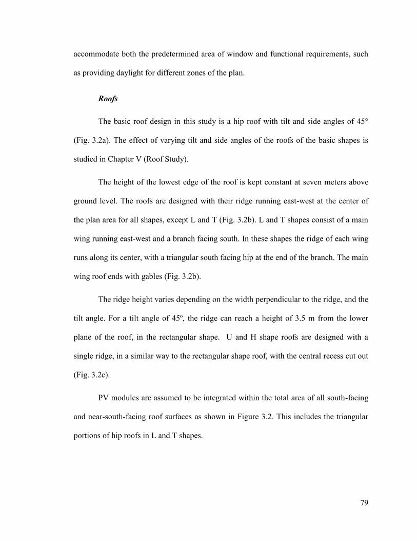
79
accommodate both the predetermined area of window and functional requirements, such
as providing daylight for different zones of the plan.
Roofs
The basic roof design in this study is a hip roof with tilt and side angles of 45°
(Fig. 3.2a). The effect of varying tilt and side angles of the roofs of the basic shapes is
studied in Chapter V (Roof Study).
The height of the lowest edge of the roof is kept constant at seven meters above
ground level. The roofs are designed with their ridge running east-west at the center of
the plan area for all shapes, except L and T (Fig. 3.2b). L and T shapes consist of a main
wing running east-west and a branch facing south. In these shapes the ridge of each wing
runs along its center, with a triangular south facing hip at the end of the branch. The main
wing roof ends with gables (Fig. 3.2b).
The ridge height varies depending on the width perpendicular to the ridge, and the
tilt angle. For a tilt angle of 45º, the ridge can reach a height of 3.5 m from the lower
plane of the roof, in the rectangular shape. U and H shape roofs are designed with a
single ridge, in a similar way to the rectangular shape roof, with the central recess cut out
(Fig. 3.2c).
PV modules are assumed to be integrated within the total area of all south-facing
and near-south-facing roof surfaces as shown in Figure 3.2. This includes the triangular
portions of hip roofs in L and T shapes.

80
Figure 3.2, Roof layouts of basic designs: a) Single ridge design for convex shapes; b) Double
ridge designs in L, T; c) Roofs of U and H shapes.
3.1.3 Parametric Investigation
The study investigates the effects of a number of parameters on the two major
response variables – solar potential and energy demand for heating and cooling. Solar
potential includes in this chapter, radiation incident on south façades and transmitted by
their windows, total heat gain from windows, and PV electricity production potential.
The thermal potential of the BIPV system (i.e. hybrid BIPV/T system) is studied in detail
in chapter V.
The parameters, whose effects on the response variable are investigated, include,
in addition to the basic shapes and south window areas, several variations to some of the
basic design configurations. These additional parameters are: variations to the geometry
S
BIPV system
BIPV
(a)
(b)
(c)
S
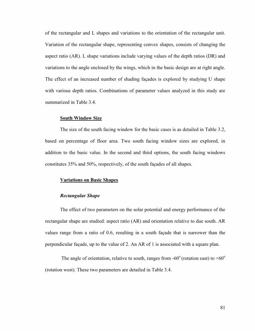
81
of the rectangular and L shapes and variations to the orientation of the rectangular unit.
Variation of the rectangular shape, representing convex shapes, consists of changing the
aspect ratio (AR). L shape variations include varying values of the depth ratios (DR) and
variations to the angle enclosed by the wings, which in the basic design are at right angle.
The effect of an increased number of shading façades is explored by studying U shape
with various depth ratios. Combinations of parameter values analyzed in this study are
summarized in Table 3.4.
South Window Size
The size of the south facing window for the basic cases is as detailed in Table 3.2,
based on percentage of floor area. Two south facing window sizes are explored, in
addition to the basic value. In the second and third options, the south facing windows
constitutes 35% and 50%, respectively, of the south façades of all shapes.
Variations on Basic Shapes
Rectangular Shape
The effect of two parameters on the solar potential and energy performance of the
rectangular shape are studied: aspect ratio (AR) and orientation relative to due south. AR
values range from a ratio of 0.6, resulting in a south façade that is narrower than the
perpendicular façade, up to the value of 2. An AR of 1 is associated with a square plan.
The angle of orientation, relative to south, ranges from -60o (rotation east) to +60
o
(rotation west). These two parameters are detailed in Table 3.4.

82
L shape Variations
L shape consists of a main wing and an attached branch. The main wing is
assumed to be oriented east-west, so as to have the long façade facing south. The branch
can be attached at either the west end, W configuration, or at the east end, E
configuration. It can also be facing south (S) or north (N). Thus the configuration L-WS,
for instance, denotes L shape with the branch attached to the west end of the main wing
towards the south (Table 3.3).
Depth Ratio
The depth of the shadow receiving facade and the number of shadow projecting
façades play an important role in determining the amount of solar radiation incident on
the shaded façade and transmitted by its windows. Two values of the depth ratio – ½ and
3/2 – are adopted for L shape, and U shape (to study the effect of two shading facades), in
addition to the basic value of 1. In the design of units with varying depth ratios, the floor
area is kept constant (ca. 60 m2). An aspect ratio of 1.3 is applied in L shape with depth
ratio of ½.
Wing Rotation
The L shape used for the study of the effect of wing rotation is characterized by a
depth ratio of ½. This ratio is selected, based on practical, functional considerations.
L variants are characterized, in addition to the depth ratio, by the angle β – the
deviation from 90o of the angle enclosed by the wings of the L (Table 3.3). Four values of
β are considered in this study – 15 o
, 30o, 45
o and 60
o. L variants are identified by the
letter V followed by a series of characters specifying the position and angle of the branch

83
(Table 3.3). For instance V-WS30 is a variant with a branch attached to the west end of
the main wing, facing south and having an angle β=30o.
An additional shape, termed hereunder Obtuse-angle (O) can be considered a
special L variant with larger values of the angle β (β=70º is adopted). For obtuse-angle
shape, the depth ratio has no significant effect as the wings, generally, do not mutually
shade. The obtuse shape may be facing in a generally south direction – O-S or north
direction – O-N.
Table 3.3. Variations of L shapes
Direction
of L
Branch
Shape
L shape Variations of L shape
L variant (V) Obtuse
angle
South
(L-WS*)
β=15º– West
(V-WS15)
β=30º – West
(V-WS30)
β=45º – West
(V-WS45)
β=60º – West
(V-WS60)
(O-S)
β=15º– West
(V-WS15)
β=30º – East
(V-ES30)
β=45º – East
(V-ES45)
β=60º – East
(V-ES60)
North
(L-WN)
β=15º – West
(V-WN15)
β=30º – West
(V-WN30)
β=45º – West
(V-WN45)
β=60º– West
(V-WN60)
(O-N)
β=15º – West
(V-EN15)
β=30º – East
(V-EN30)
β=45º – East
(V-EN45)
β=60º – East
(V- EN60)
*Solar potential and energy demands of L-E and L-W are not significantly different (with L-W performing
slightly better than L-E)
a
b
β

84
Obtuse angle and trapezoid shapes typically feature in sites of curved layout,
covered in Chapter IV. Trapezoid is analyzed in this chapter as a basic shape (angle θ=
60°, Fig. 3.1). In chapter IV it features (with a different geometry) in attached
configurations in sites of curved layout. Obtuse angle is studied in this chapter for south
and north orientations, as shown in Table 3.3.
A photovoltaic system is assumed to cover all south and near-south facing roof
surfaces, including the triangular portions of hip roofs in L shape and its variants, and the
two near south facing surfaces in obtuse-angle roofs. Figure 3.3 presents roofs of selected
L variants and the BIPV portion of the roofs.
Figure 3.3, Irregular roof shapes and PV integration. PV integrated surfaces are shown
hatched. a) and b) represent roofs of V-WS60- variant and obtuse angle O-S, c) and d) represent V-
EN60 and O-N.
Summary of Parametric Investigation
Values of the parameters investigated in the study of dwelling shapes are
summarized in Table 3.4. These parameters consist mainly of the basic shapes and
variations on the rectangular, L and U shapes. A total of 30 configurations of parameter
(
a)
(
b)
(
c)
(d)
BIPV
(c)
(b) (a)

85
combinations are designed and investigated. This is in addition to a large number of
scenarios designed to identify the effect of single independent design parameters that are
decoupled from others (e.g orientation, aspect ratio, south window area (as fixed area or
as percentage of the south façades), etc.).
Table 3.4, Parameter combinations
3.2 Presentation and Analysis of Results
Simulations are performed to analyze the effect of the design parameters detailed
above on solar potential and heating and cooling loads and consumption (assuming a heat
pump of COP 4). Assumptions employed in the simulations are detailed in Chapter II.
The effects of basic shape design are first presented, followed by the analysis of
variations to the basic designs.
Shape Aspect ratio
(AR)
Orientation Depth
ratio
(DR)
Rotation of
branch
(L shape)
South facing window
area
Basic shapes (Fig.2) Basic South Basic
design
n/a 10% of total floor
area
35% of south façade
50% of south facade
Var
iati
on
s o
f sh
apes
Rectangle 1-2 (step of
0.1)
South n/a n/a 35% of south façade
1.3 -60
o to +60
o n/a n/a
L
shape
L Basic South and North
(see Table 3.3)
1/2- 3/2 n/a
L variants 1.3 South and North
(see Table 3.3)
1/2 β=15º-60 º (15 º
step)
Obtuse
Angle
1.2 South and North
(see Table 3.3)
1/2 β=70º

86
3.2.1. Effects of Basic Shape Design
Solar Potential
Solar Radiation and Heat Gain
The mean daily global insolation for the south facing non-shaded façade obtained
from EnergyPlus simulations is about 3.23kWh/m2. This value falls within the range
estimated by Natural Resources Canada (NRCan) (2.5-3.3 kWh/m2) for the studied
location (NRCcan, 2011).
The results include allowance for shading in non-convex shapes such as L, U, H
and T. The total radiation is compared with radiation on the rectangular shape, which
serves as reference. Figure 3.4 displays the total transmitted radiation (in kWh) for a
single south facing window unit (2 m2), for both shaded and non-shaded façades, for the
winter and summer design days. It should be noted that for the basic cases, where the
south facing windows are considered as percentage of the floor area, the total area of
south-facing windows is the same for all shapes. Following are some comments on the
more significant results.
In the absence of shading in convex shapes, the amount of radiation incident and
transmitted by windows depends solely on the size of the south façade and
windows.
For non-convex shapes, an additional factor that influences solar radiation is the
shade cast by adjacent façades. The reduction of incident radiation on the south
shaded façade of the basic non-convex shapes as compared to the rectangle
amounts to 22% for the L shape and 43% for the U shape (DR=1) (Fig. 3.4). A

87
similar effect is observed for the transmitted radiation by windows of the south
façades of L and U shapes. This effect is studied below in more detail.
Heat gain through windows in convex shapes is affected only by the size of the
windows. In non-convex shapes, solar heat gain is affected by shading
parameters in addition to window size. Figure 3.5 presents the annual solar heat
gain associated with different window size options for each of the shapes. It can
be observed that while for the basic window size (10% of the floor area) shape
effect is not significant, heat gain for windows of 35% and 50% of façade area is
strongly affected by shape.
Figure 3.4, Transmitted radiations by windows in south façades for a WDD and for a SDD.
0.00
1.00
2.00
3.00
4.00
5.00
6.00
Cube Rectangle Trapezoid Lshape Ushape Hshape Tshape
WDD-non-shadedfacade(kWh) 5.68 5.68 5.68 5.68 5.68 5.68 5.68
WDD-shaded facade(kWh) 4.17 3.07 5.67 4.79
SDD-shaded facade (kWh) 1.51 1.14 1.79 1.59
SDD-non shaded facade 1.86 1.86 1.86 1.86 1.86 1.86 1.86
Transmitted radiation
(kWh)
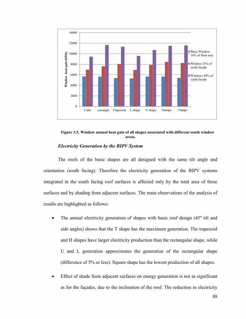
88
Figure 3.5, Window annual heat gain of all shapes associated with different south window
areas.
Electricity Generation by the BIPV System
The roofs of the basic shapes are all designed with the same tilt angle and
orientation (south facing). Therefore the electricity generation of the BIPV systems
integrated in the south facing roof surfaces is affected only by the total area of these
surfaces and by shading from adjacent surfaces. The main observations of the analysis of
results are highlighted as follows:
The annual electricity generation of shapes with basic roof design (45º tilt and
side angles) shows that the T shape has the maximum generation. The trapezoid
and H shapes have larger electricity production than the rectangular shape, while
U and L generation approximates the generation of the rectangular shape
(difference of 5% or less). Square shape has the lowest production of all shapes.
Effect of shade from adjacent surfaces on energy generation is not as significant
as for the façades, due to the inclination of the roof. The reduction in electricity
0
2000
4000
6000
8000
10000
12000
14000
Cube rectangle Trapezoid L shape U shape Hshape Tshape
Win
do
w h
ea
t g
ain
(k
Wh
) Basic Window-
10% of floor area
Window 35% of
south facade
Windows 50% of
south facade

89
generation reaches a maximum of 6% per m2, averaged over the roof area, for
the basic L shape.
U and H shape roofs are not affected by the number of shading façades and the
DR in the studied cases, due to the roof design adopted in these cases (Fig. 3.2c).
Figure 3.6 presents the winter design day (WDD) peak electricity generation and
the annual energy generation associated with all basic shapes. A comparison of the
annual electricity generation of the BIPV system of each shape to the reference case
(rectangle) is presented in Table 3.5, which gives a summary of energy performance of
all basic shapes.
Figure 3.6, WDD peak electricity generation and annual electricity generation for all basic
shapes.
Energy Demand
The effect of basic shape of units on the energy demand is first determined by
analyzing the effect of the building envelope. The results indicate a correlation between
heating energy demand and the total building envelope area – Fig. 3.7. The correlation
between heating load and the building envelope area is inversely proportional to window
area. Heating and cooling loads of all basic shapes and the comparison of heating load of
WD
D p
eak e
lect
rici
ty g
ener
atio
n (
kW
)

90
these shapes to the reference are presented in Table 3.5. Energy balance between
production and total energy consumption is discussed in section 3.2.3.
Figure 3.7, Correlation between building envelope area and heating load for varying ratios of south
facing window areas.
Table 3.5, Energy performance of basic shapes
The annual heating and cooling loads associated with various south window areas
are presented in Table 3.6 and in Figure 3.8. Heating load is reduced dramatically for
shapes like U and H (about 35%) when the south window constitutes 50% of the façade,
as compared with the basic cases.
1000
1500
2000
2500
3000
3500
4000
4500
5000
305
Square
304
Rectangle
324
Trapezoid
336
L shape
346
Tshape
419
U shape
443
Hshape
Hea
tin
g L
oad
(k
W)
Building envelope surface (m2)/
shape
Basic cases
Windows 35%
50% of south
facade
35% of south
facade
South
window area
Total
envelope
area (m2)
South
facing
roof area
(m2)
Yearly
window
heat gain
(kWh)
Yearly
Heating
load (kW)
Yearly
Cooling
load (kW)
Yearly
Energy
generation
(kWh)
Ratio of
heating
load to
reference
Ratio of
energy
generation to
reference
Square 305 21.8 5685 3024 110 4233 0.99 0.87
Rectangle 304 25.6 5652 3041 107 4867 1 1
Trapezoid 325 34 5383 3287 90 6777 1.08 1.37
L shape 336 27.4 5304 3581 106 4948 1.20 1.014
U shape 390 24.7 5682 3780 106 4835 1.24 0.99
H shape 443 31.5 5656 4460 74 6168 1.47 1.26
T shape 346 37 5424 3693 79 7228 1.21 1.48

91
Increasing the south window area to 50% of the total south façade leads to an
increase in the cooling load. This increase is particularly significant for the rectangular
and trapezoid shapes. Cooling load constitutes 31% and 24% of their heating load,
respectively. It should be noted however that cooling load for the basic cases is lower by
over an order of magnitude than the heating load, and the design should therefore aim at
minimizing heating load, in climatic conditions similar to those employed in this
research.
Table 3.6, Effect of window size on annual heating and cooling loads of basic shapes
Heating energy consumption is computed assuming a heat pump of coefficient of
performance (COP) of 4. Figure 3.8 displays the heating energy consumption of all
shapes, associated with each window area option.
Shapes
Basic south window (10% of
floor area) Window 35% of south facade Window 50% of south facade
Heating
load
(kW)
Cooling
load
(kW)
Ratio of
cooling to
heating
load
Heating
load
(kW)
Cooling
load
(kW)
Ratio of
cooling to
heating
load
Heating
load
(kW)
Cooling
load
(kW)
Ratio of
cooling to
heating
load
Square 3024 110 0.04 2662 173 0.07 2193 371 0.17
Rectangle 3041 107 0.04 2511 212 0.08 1983 624 0.31
Trapezoid 3287 90 0.03 2536 211 0.08 2045 499 0.24
L shape 3581 106 0.05 3062 162 0.05 2616 379 0.15
U shape 4200 106 0.03 3473 170 0.05 2688 454 0.17
H shape 4464 74 0.02 3566 182 0.05 2899 392 0.14
T shape 3693 79 0.02 2919 233 0.08 2453 542 0.22
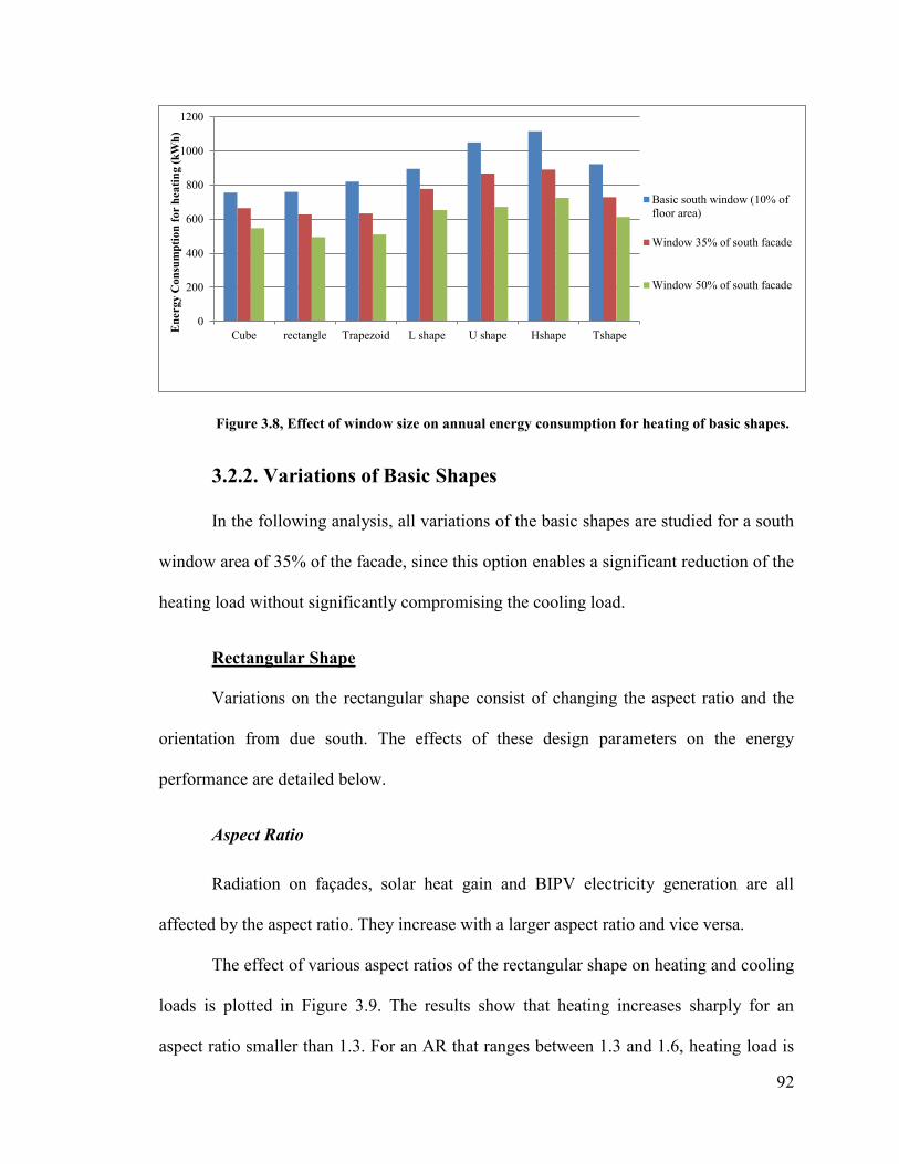
92
Figure 3.8, Effect of window size on annual energy consumption for heating of basic shapes.
3.2.2. Variations of Basic Shapes
In the following analysis, all variations of the basic shapes are studied for a south
window area of 35% of the facade, since this option enables a significant reduction of the
heating load without significantly compromising the cooling load.
Rectangular Shape
Variations on the rectangular shape consist of changing the aspect ratio and the
orientation from due south. The effects of these design parameters on the energy
performance are detailed below.
Aspect Ratio
Radiation on façades, solar heat gain and BIPV electricity generation are all
affected by the aspect ratio. They increase with a larger aspect ratio and vice versa.
The effect of various aspect ratios of the rectangular shape on heating and cooling
loads is plotted in Figure 3.9. The results show that heating increases sharply for an
aspect ratio smaller than 1.3. For an AR that ranges between 1.3 and 1.6, heating load is
0
200
400
600
800
1000
1200
Cube rectangle Trapezoid L shape U shape Hshape Tshape
En
erg
y C
on
sum
pti
on
fo
r h
ea
tin
g (
kW
h)
Basic south window (10% of
floor area)
Window 35% of south facade
Window 50% of south facade
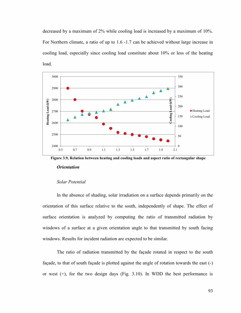
93
decreased by a maximum of 2% while cooling load is increased by a maximum of 10%.
For Northern climate, a ratio of up to 1.6 -1.7 can be achieved without large increase in
cooling load, especially since cooling load constitute about 10% or less of the heating
load.
Figure 3.9, Relation between heating and cooling loads and aspect ratio of rectangular shape
Orientation
Solar Potential
In the absence of shading, solar irradiation on a surface depends primarily on the
orientation of this surface relative to the south, independently of shape. The effect of
surface orientation is analyzed by computing the ratio of transmitted radiation by
windows of a surface at a given orientation angle to that transmitted by south facing
windows. Results for incident radiation are expected to be similar.
The ratio of radiation transmitted by the façade rotated in respect to the south
façade, to that of south façade is plotted against the angle of rotation towards the east (-)
or west (+), for the two design days (Fig. 3.10). In WDD the best performance is
0
50
100
150
200
250
300
350
2400
2500
2600
2700
2800
2900
3000
0.5 0.7 0.9 1.1 1.3 1.5 1.7 1.9 2.1
Co
oli
ng
Lo
ad
(k
W)
Hea
tin
g L
oa
d (
kW
)
Heating Load
Cooling Load

94
associated with the south orientation and it is reduced by 50% when the orientation angle
approaches 60º west or east from south. By contrast, for the SDD, the transmitted
radiation increases with increasing rotation angles (up to 60%) (Fig. 3.10).
Figure 3.10, Effect of orientation on transmitted radiation over a summer and winter design
day (SDD and WDD).
The effect of the orientation of roof surfaces on electricity generation, in the
absence of shading, is independent of shape. This effect is studied in detail in Chapter V
(Roof study). Following is a summary of the main effect of the orientation on the basic
hip roof (with 45° tilt angle) of the rectangular shape.
For the WDD, the best performance of the BIPV is associated with the south
orientation and it declines sharply, when the orientation exceeds 30º of true
south.
For the SDD, an increase of about 25% of electricity generation can be achieved
with an orientation of 60° towards the west. This is due to the long daylight
period, with high solar intensity in the afternoon.
Ra
tio
to
ra
dia
tio
n t
ran
smit
ted
by
so
uth
faci
ng
win
do
w o
f th
e re
cta
ng
le

95
Annually, the highest energy yield is associated with a south facing BIPV
system. Deviation of the orientation of the system from the south by up to 45°
west or east leads to an approximate reduction of 5% of the annual generation of
electricity. A rotation of the system by 60°, west or east of south, results in a
reduction of some 12% of the total annual electricity generation.
Orientation of the PV system towards the east or west results in shifting the time
of peak electricity generation. Shift of peak generation enables more overlap with
the utility grid. Detailed discussion of this issue is provided in Chapter V.
Energy Demand
The annual heating load for rectangular units is determined as function of their
orientation from due south (Fig 3.11). The results indicate that both heating and cooling
loads increase with increased angles of rotation. The heating load is increased by up to
30% with a rotation angle of 60° east or west from south, as compared to the south facing
rectangular shape. Cooling load increases significantly with the orientation toward east
or west. An increase of 65% is associated with an orientation of 60° from due south. This
increase in cooling load is mainly due to the large window area on the south-east or
south- west facade, which was originally intended to be south facing.
Figure 3.11, Heating load of rectangular units with various orientations.
1500
2000
2500
3000
3500
60E 45E 30E 20E 0 20W 30W 45W 60W
Hea
tin
g L
oa
d (
kW
)
Orientation

96
Non- Convex Shapes
Variations of non-convex shapes are studied for L shape, where the effect of
changing the depth ratio and the angle between the wings is investigated. L shape can be
considered as the basic non-convex shape and other non-convex shapes can be derived y
combinations/variations of this shape.
In addition, U shape is briefly analyzed to study the effect of increasing the
number of shading façades associated with different depth ratios on the solar radiation
incident on the façades and transmitted by their windows. Other aspects of energy
performance of U shape variations are not explored, due to the difficulty to realize a
functional plan design for U shape with other depth ratios, under the design conditions
and the floor area limitations employed in this research.
Depth Ratio
Solar Potential
Solar radiation incident on the shaded façade of a non-convex shape is
significantly dependent on the depth ratio. Another important effect is the number of
shading façades.
The effect of depth ratio on incident and transmitted solar radiation of U and L
shapes for a winter design day is shown in Table 3.7. Following are the main
observations:
The results indicate that the average radiation, per m2, incident on the shaded
south façade of L shape is reduced by 12%, 22% and 26%, for depth ratio values

97
of 1/2, 1 and 3/2, respectively, as compared to the radiation on the exposed south
façade.
The reduction of the average incident radiation on the south facing shaded façade
of U shape, and transmitted by its window is approximately double that of the
corresponding L shape (with similar depth ratios) (Table 3.7).
Table 3.7, Effect of depth ratio on incident and transmitted radiation of L and U shapes
shape Number of shade projecting façades a/b=1/2 a/b=1 a/b=3/2
L shape 1
Reduction of average radiation on shaded
façade 12% 22% 26%
Reduction of average transmitted radiation 7% 27% 34%
U shape 2
Reduction of average radiation on shaded
façade 23% 43% 53%
Reduction of average transmitted radiation 14% 46% 60%
The effect of depth ratio on electricity generation is analyzed only for L shape
since U shape is designed with a roof similar to the rectangular shape, with no shading
effect.
Electricity generation is affected only slightly by the depth ratio, due to the
inclination of the roof which reduces the shading effect. For instance, the electricity
generation of the basic L shape (with depth ratio =1) is reduced annually by a maximum
of 6% when averaged per unit area, as compared with the electricity generated per unit
area of a non-shaded south facing roof. The maximum difference in annual electricity
generation per unit area of L shape for the different depth- ratios studied is 3% or less.
Energy Demand
The depth ratio effect on energy demand is coupled with other effects such as the
aspect ratio, which changes with different depth ratios in order to maintain the same plan

98
area, and south facing window area, which changes as percentage of the facade.
Therefore it is difficult to isolate the effect of depth ratio on energy demand for heating
and cooling.
The effect of depth ratio (including the design issues mentioned above) are shown
in Table 3.8. L shape with DR of ½ requires 9% less heating than L shape with DR of 1
(and about 7% more than the rectangle). The effect of DR on incident radiation on the
shaded south façade as compared to the rectangular shape is presented in Table 3.8 as
well.
Table 3.8, effect of DR on solar potential and energy performance
DR
Window heat
gain (103.kW)
Percentage of
reduced incident
radiation (WDD)
Heating load
(kW)
Cooling load
(kW)
Electricity
generation
(kWh)
1/2 8244 12% 2686 259 5840
1 7904 22% 3062 162 4958
3/2 7328 26% 3165 155 4111
Wing Rotation in L Variants (V)
Solar Potential
L variants (V) are designed with a DR of ½. The effect of wing rotation on solar
potential is assessed by comparison to the rectangle.
Two main observations are highlighted in the analysis of the incident and
transmitted solar radiation of L variants:
A larger angle between the wings of L shape allows reducing the shade on the
main wing (shaded façade), and therefore increasing transmitted radiation and
windows heat gain. The reduction of solar radiation on the shaded façade is not
significant when the angle β is larger than 30° (≤1%) for the depth ratio of 1/2.

99
Rotation of the south facing façade of the branch of L shape causes an increase of
the incident radiation on this facade, for the SDD and decrease of this radiation
for the WDD. This effect of rotation of the wing on incident/transmitted radiation
follows the same principles detailed in the analysis of the effect of orientation on
the solar potential of the rectangular shape presented above and depicted in
Figure 3.10.
The annual electricity generation of selected south facing L variants (V-ES and V-
WS) and north facing L variants (V-EN and V-WN), with a depth ratio of ½, is compared
to the rectangle in Table 3.9. Figure 3.12 displays the annual electricity generation of
these selected shapes. The main observations of L variations effect on electricity
generation are as follows:
The shade on the south facing roof in all non-convex shapes is mitigated by a
small depth ratio as well as by increased angle between the wings. Consequently
the electricity generation potential in such units is not significantly affected by
shading.
The L and L variant shapes provide larger roof area, than the reference case
(rectangle with a hip roof) and therefore an increase in annual electricity
generation.
The comparison of the annual electricity production of south facing L variants
indicates an increase of the annual generation ranging from 20% to 35% relative
to the reference case. This effect is attributed to the larger south facing roof area
(31m2 for the L variant, in comparison with 25.6m
2 for the rectangular shape).

100
The increase in total annual generation of the north facing L variant (V-WN60),
relative to the reference, can reach 53%. North facing obtuse-angle shape
generates up to 30% more electricity annually than the reference.
Table 3.9, Comparison of annual electricity generation of selected L variants to the reference
case
South facing Rectangle V-ES60 V-ES30 L-WS/L-ES V-WS30 V-WS60 O-S
Comparison to
reference 1 1.35 1.26 1.22 1.26 1.38 1.10
North facing Rectangle
V-
EN60 V-EN30 L-WN/L-EN V-WN30 V-WN60 O-N
Comparison to
reference 1 1.50 1.18 1.32 1.18 1.53 1.30
(a)
(b)
Figure 3.12, Annual energy production of selected L variants, (a) South Facing (V-ES and V-
WS), (b) North Facing (V-EN and V-WN).
0
1000
2000
3000
4000
5000
6000
7000
Rectangle V-ES60 V-ES30 L-ES shape V-WS30 V-WS60 O-S
An
nu
al
en
erg
y p
ro
du
cti
on
(k
Wh
)
0
1000
2000
3000
4000
5000
6000
7000
8000
Rectangle V-EN60 V-EN30 L -ENshape V-WN30 V-WN60 O-N
An
nu
al
en
erg
y g
en
era
tio
n (
kW
h)

101
Peak Generation Timing
The hourly electricity generation during the WDD indicates that the different
variations of L shape allow reaching the peak at different times, as shown in Figures
3.13a and 3.13b for L variants with south facing wings. The peak generation is reached
earlier than solar noon for V-ES variants and later for V-WS variants. Figures 3.13a and
3.13b show the normalized peak generation per unit area of different variations of L
shape on a WDD and SDD respectively. A difference of peak of about 3 hours is
observed between L variation with β=30º east (peak between 11 – 12 hours) and the
variation with β=30º west (peak between 13 – 14 hours).
A maximum shift of 3 hours relative to solar noon can be obtained by the BIPV
system of L variants with 60°-70° wing rotation. This is discussed in detail in chapter V.
(a)
9 10 11 12 13 14 15 16 17 18 19 20 21
Lshape 0 5 46 79 100 111 111 99 66 26 1 0 0
15ºE 0 7 55 87 105 111 106 90 57 20 1 0 0
30ºE 0 8 61 92 105 106 97 77 45 13 0 0 0
45ºE 0 8 63 91 101 97 84 62 32 7 0 0 0
60ºE 0 8 62 85 90 82 66 43 17 3 0 0 0
15ºW 0 3 35 67 91 106 111 105 88 55 6 0 0
30ºW 0 1 22 52 78 96 106 105 92 61 7 0 0
45ºW 0 0 9 35 61 83 97 100 91 63 8 0 0
60ºW 0 0 3 16 42 65 81 89 85 61 8 0 0
0
20
40
60
80
100
120
En
erg
y g
ener
ati
on
(W
/m2)
Time (hr)
Lshape
15ºE
30ºE
45ºE
60ºE
15ºW
30ºW
45ºW
60ºW

102
(b)
Figure 3.13, Electricity generation for L shape with wing rotation (kW/m2), (a) WDD, (b)
SDD.
Energy Demand
Heating load (and heating consumption determined assuming a heat pump of COP
4) is not significantly affected by wing rotation of L variants. L shape, south facing L
variants with angle β =60° (V-ES60 and V-WS60), and obtuse angle shape (OS) require
7%, 6% and 2% respectively, more heating energy than the reference case (rectangle).
The cooling load of L variants exceeds that of the reference case by up to 30%
(associated with an angle β of 60°). This is caused by increased transmitted radiation in
the morning and evening during the summer period, by windows that are originally
designed as south facing. This effect can be mitigated by modifying the window area, on
the rotated façade. This is not investigated however in this research in order to avoid
introducing additional design parameters.
North facing L variants (V-EN, V-WN) require more energy for heating than the
corresponding south facing (V-ES, V-WS). For instance the increase of heating load of
En
erg
y g
ener
atio
n (
W/m
2)
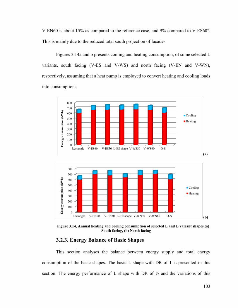
103
V-EN60 is about 15% as compared to the reference case, and 9% compared to V-ES60°.
This is mainly due to the reduced total south projection of façades.
Figures 3.14a and b presents cooling and heating consumption, of some selected L
variants, south facing (V-ES and V-WS) and north facing (V-EN and V-WN),
respectively, assuming that a heat pump is employed to convert heating and cooling loads
into consumptions.
(a)
(b)
Figure 3.14, Annual heating and cooling consumption of selected L and L variant shapes (a)
South facing, (b) North facing
3.2.3. Energy Balance of Basic Shapes
This section analyses the balance between energy supply and total energy
consumption of the basic shapes. The basic L shape with DR of 1 is presented in this
section. The energy performance of L shape with DR of ½ and the variations of this
0
100
200
300
400
500
600
700
800
Rectangle V-ES60 V-ES30 L-ES shape V-WS30 V-WS60 O-S
En
erg
y c
on
sum
pti
on
(k
Wh
)
Cooling
Heating
0
100
200
300
400
500
600
700
800
Rectangle V-EN60 V-EN30 L -ENshape V-WN30 V-WN60 O-N
En
erg
y c
on
sum
pti
on
(k
Wh
)
Cooling
Heating

104
shape (studied in section 3.2.2), are presented in Chapter IV together with the energy
balance of the studied neighborhood patterns.
The total consumption of electricity for lighting, DHW and appliances, in addition
to the computed heating and cooling energy consumption, for each basic shape is detailed
in Table 3.10 and depicted in Figure 3.15 alongside the energy production of the
corresponding units. The results, in terms of percentage of energy production to energy
consumption of all shapes, are also presented in Table 3.10.
The results indicate that the electricity production of the reference rectangular
layout with hip roof falls short by some 35% of its energy consumption. T shape
produces up to 95% of total consumption, meaning that this shape is very close to
achieving a net zero energy status, even though it consumes about 9% more heating
energy then the rectangular shape.
It should be noted that energy consumption for lighting in this research is
considered as the same for all shapes. However lighting in some non-convex shapes,
particularly in L and T shapes can be further reduced if additional daylight considerations
are accounted for, due the benefit of the shallow depth of these shapes. This is to be
investigated in future research. Thermal potential of a hybrid photovoltaic thermal
system, which is investigated in detail in Chapter V, is expected to further reduce energy
consumption for space and water heating and for some appliances (clothes drier, for
instance).

105
Table 3.10, Energy consumption for all basic units
Square Rectangle Trapezoid L shape U shape H shape T shape
Heating energy consumption
(kWh) 665 627.6 634 765 868 891 730
Cooling energy consumption
(kWh) 43 53 53 40 42 45 58
DHW (kWh) 3786 3786 3786 3786 3786 3786 3786
Appliances (kWh) 2700 2700 2700 2700 2700 2700 2700
Lighting (kWh) 360 360 360 360 360 360 360
Total Energy use (kWh) 7554 7526 7532 7664 7756 7782 7633
Annual electricity generation
(kWh) 4233 4887 6777 4958 4835 6168 7228
Ratio Energy supply/energy
use 0.56 0.66 0.90 0.65 0.62 0.79 0.95
Figure 3.15, Energy use and energy supply of all basic shapes.
0
1000
2000
3000
4000
5000
6000
7000
8000
Ele
ctri
city
gen
era
tio
n a
nd
en
erg
y
con
sum
pti
on
(k
Wh
) Annual energy
generation
Lightig
Appliances
DHW
Cooling
Heating

106
Chapter IV: Neighborhood design2
The objective of this chapter is to assess the effects of a variety of parameters
associated with residential neighborhood design on the solar performance and energy
balance of a neighborhood and of the individual housing units composing it. The two
main parameters affecting neighborhood solar performance are the site layout and the
density of housing units. Each of these parameters is associated and interacts with several
secondary parameters, such as units’ shapes, their orientation, their relative position etc.
The selection of housing shapes for the neighborhood investigation is based on results
obtained in the investigation of shape effects (Chapter III).
The chapter includes two main sections. Section 4.1 presents the design
parameters selected in this study and the values assigned to them. Section 4.2 presents
results and evaluation of the simulation analysis, in terms of the effects of the design
parameters on solar potential and energy consumption of units in a neighborhood and the
energy performance of the neighborhood as a whole.
4.1 Design Parameters
This section details the parameters considered in the neighborhood investigation,
their values and the various combinations studied. It comprises four main subsections.
The general neighborhood characteristics and site layouts are presented in section 4.1.1.
2 The study and some of the results presented in this chapter are published in:
Hachem C., A. Athienitis, P. Fazio, (2012a). Evaluation of energy supply and demand
in solar neighbourhoods, Journal of Energy and Buildings,DOI: 10.1016/j.enbuild.2012.02.021.
Hachem C., A. Athienitis, P. Fazio, (2011b), Investigation of Solar Potential of Housing Units in
Different Neighborhood Designs, Journal of Energy and Buildings, Volume 43, Issue 9, Pages 2262-2273.

107
Section 4.1.2 introduces the main parameters associated with mutual shading by adjacent
housing units in a neighborhood. Values of neighborhood design parameters are detailed
in section 4.1.3, under three main headings, representing the three categories of design
parameters: unit shapes; density and site layout. Section 4.1.4 presents a summary of the
parametric investigation, including the combinations of parameter values analyzed.
4.1.1. Neighborhood Characteristics
The general characteristics of the neighborhood are based on various sources,
including guidelines of urban design and by- law zoning (e.g. CWP, 1998; Cohen, 2000;
Burden et al, 1999). Table 4.1 summarizes the neighborhood design guidelines adopted in
this study. The design methodology consists of first determining the site layout, then
designing the unit shapes to conform to this layout, and combining the shapes in different
configurations.
Table 4.1, Characteristics of the studied neighborhoods
Land use
designed
Building total floor area 120 m2
(designed )
Lot Coverage Ratio (
) 37% (calculated)
Distance
from sides
Front 4m
Back 6m
Sides Units positioned with respect to a straight
road
2m
Units positioned with respect to curved road 2 - 3.5m
Roads
based on
(CWP, 1998,
Cohen, 2000,
Burden et al,
1999)
Road width Neighborhood streets a
12 -15m Gravel alley
b 4m
Cul de sac Diameter see Table 4.3 D1=42 m
D2=52m
Density
(based on
Teed et al.,
2009)
Low/ medium -Low - outer suburban area (detached units-see Table
4.3)
5-9 u/a
Medium- high -outer suburban area (attached units see Table 4.3) 16 u/a
Medium- inner suburban (row townhouse see Table 4.3) up to 35 u/a a Access to residential, includes street width with parking on one or two sides, planting strip, sidewalks on
both side. b Access to sanitation and utilities, garages, backyard and secondary units.

108
Three basic site layouts are considered in this study (see Fig. 2.5, Chapter II). Site
I is characterized by a straight road, while sites II and III feature curved roads facing
south and north, respectively. Variations on site I are also designed to find the effect of
varying straight road orientations.
For each site, several configurations consisting of combinations of groups of three
to six units of a given shape are studied. For each site/shape combination, three densities
are considered: low density (around 5 units per acre (u/a)), medium -low density (around
9 units per acre (u/a)) of detached units (Teed et al, 2009) and medium- high density
(around 16 (u/a)) consisting of attached units (Table 4.1). In site I, the effect of mutually
shading rows of dwelling units, in what is termed row effect, is also studied. A higher
density of up to 35 u/a can be achieved employing row configurations.
4.1.2 Shading Effects
A major effect on solar potential of neighborhoods is mutual shading by adjacent
dwelling units. Two parameters define the relative position of the shaded and shading
units: the angle of obstruction and the distance between the units.
Planar Obstruction Angle (POA) is a new concept introduced in this research
representing the angle between the center of the south façade of the shaded unit and the
closest corner of the shading unit (Figs. 4.1 and 4.2). In the analysis of POA effects, POA
values of 15°, 30°, 45°, 60°, 75° and 90° are studied, in addition to the effect of aligning
the units, as shown in Figure 4.1.
The second parameter is the distance (d) from the center of the south façade of the
shaded unit to the closest corner of the obstructing unit. Four values of d are adopted in
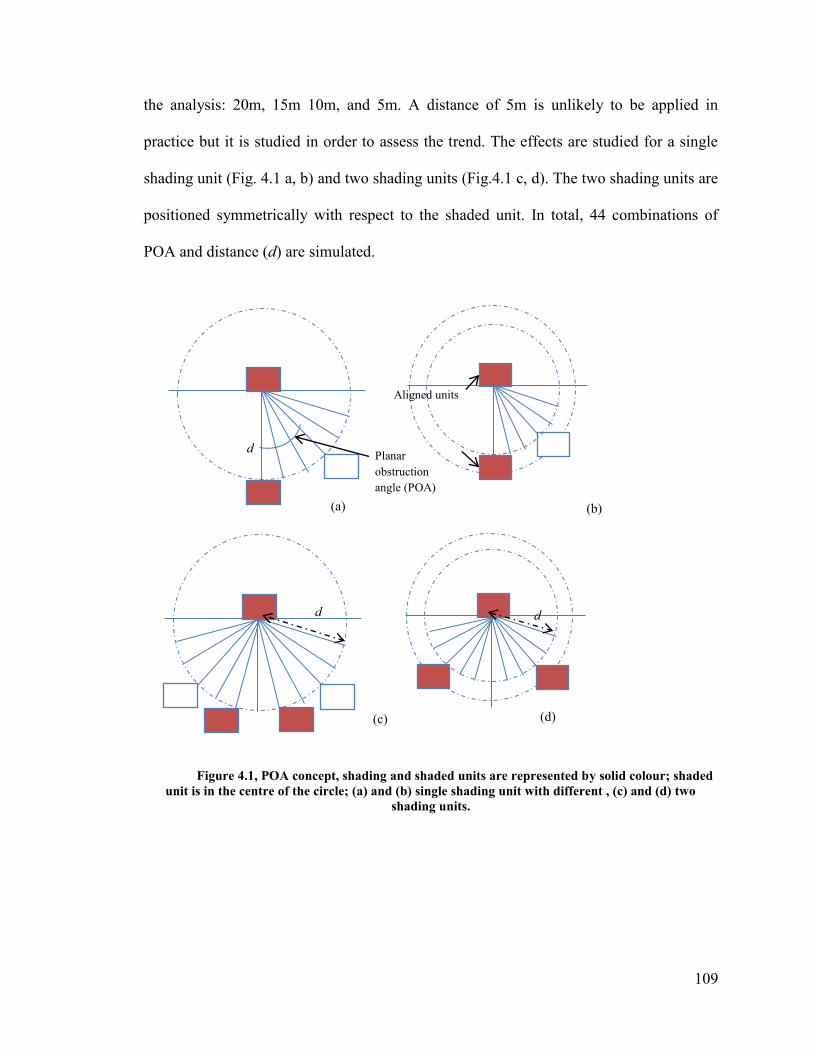
109
the analysis: 20m, 15m 10m, and 5m. A distance of 5m is unlikely to be applied in
practice but it is studied in order to assess the trend. The effects are studied for a single
shading unit (Fig. 4.1 a, b) and two shading units (Fig.4.1 c, d). The two shading units are
positioned symmetrically with respect to the shaded unit. In total, 44 combinations of
POA and distance (d) are simulated.
Figure 4.1, POA concept, shading and shaded units are represented by solid colour; shaded
unit is in the centre of the circle; (a) and (b) single shading unit with different , (c) and (d) two
shading units.
(a)
Planar
obstruction
angle (POA)
(b)
(c)
d1
(d)
d
2
Aligned units
d
d
d

110
(a) (b)
Figure 4.2, 3-D view of the POA concept, (a) one shaded unit, (b) 2 shaded units.
4.1.3 Neighborhood Design Parameters and their Values
Housing Units’ Shapes
Rectangle and L shape and its variations are selected for the neighborhood study,
since they can be considered as prototypes of convex and non-convex shapes for passive
solar design. Other basic shapes can be derived from combination / variation of these
shapes. Non-convex dwelling units employed in the neighborhood study are shown in
Table 3.3 (Chapter III). Details of the design and analysis of all shapes considered in this
research are provided in sections 3.1.1 and 3.1.3 of Chapter III.
Site Layout
Site layout is mainly characterized by the layout of streets. Two main street
layouts are studied: straight, and semi- circular.
Straight Road – Site I
Six directions of the straight road are studied, in addition to the reference case ‒
an east-west running road (Fig. 4.4.a), with the E-W road rotated by 30°, 45° and 60° in
each of clockwise (+) and anticlockwise (-) senses. Only detached configurations are
r
2
r
1

111
studied in these inclined configurations, since the purpose is to study the effect of mutual
shading, which is not relevant to attached units.
For each of the inclined layouts of site I, 3 housing units’ configurations are
studied: south facing rectangle, rectangle oriented toward the street, and L variants (V),
with the angle between the wings to conform to road direction. Figure 4.3 shows sites
with +45° orientation (rotation towards the west) of the three configurations mentioned
above.
Figure 4.3, variation of site I, (a) south facing rectangle, (b) rectangles oriented to the street,
(c) L-variants (V).
Curved road – Sites II and III
Site layout II and III incorporate semi-circular roads, facing south and north,
respectively. The housing units are positioned with respect to the shape of the roads, in
both curved sites. Configurations of site II include rectangular shape (R), combination of
L shape and its variants and a configuration of obtuse-angle shapes (Fig. 4.4b). In the last
configuration (Obtuse angle) the two extreme units – U1 and U5 in Fig. 4.4b ‒ are L
variants (V-ES60 and V-WS60), in an attempt to optimize façade orientation for
insolation. Configurations of site III are mirror images of those of site II, relative to an
east-west axis (Fig. 4.4c).
S
45°
POA r
(a) (c) (b)
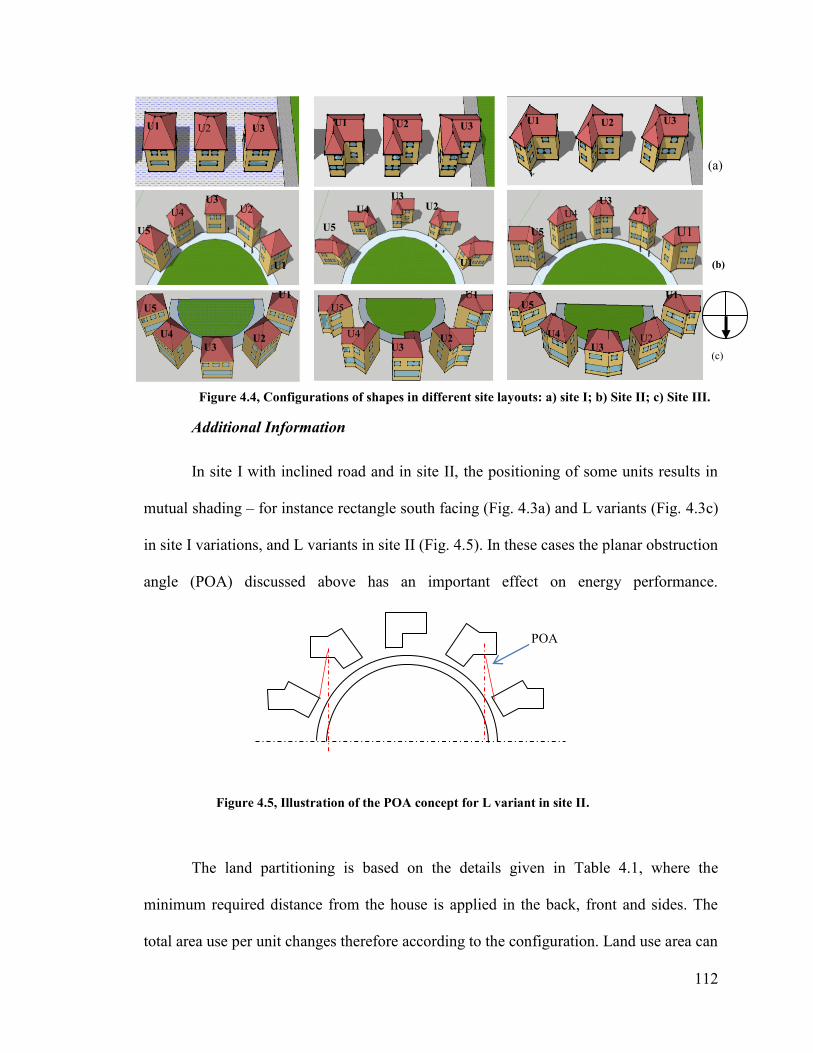
112
Figure 4.4, Configurations of shapes in different site layouts: a) site I; b) Site II; c) Site III.
Additional Information
In site I with inclined road and in site II, the positioning of some units results in
mutual shading – for instance rectangle south facing (Fig. 4.3a) and L variants (Fig. 4.3c)
in site I variations, and L variants in site II (Fig. 4.5). In these cases the planar obstruction
angle (POA) discussed above has an important effect on energy performance.
The land partitioning is based on the details given in Table 4.1, where the
minimum required distance from the house is applied in the back, front and sides. The
total area use per unit changes therefore according to the configuration. Land use area can
POA
Figure 4.5, Illustration of the POA concept for L variant in site II.
(c)
(a)
U2
U1
U5
U4
U3 U2
U1
U5
U4
U3
U2
U1 U5
U4
U3
U2
U1
U5
U4
U3 U2
U1
U5
U4
U3 U2
U1 U5
U4
U3
(b)
S
U3 U2 U1 U1 U3 U2 U1 U3 U2
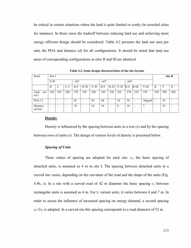
113
be critical in certain situations where the land is quite limited or costly (in crowded cities
for instance). In these cases the tradeoff between reducing land use and achieving more
energy efficient design should be considered. Table 4.2 presents the land use area per
unit, the POA and distance (d) for all configurations. It should be noted that land use
areas of corresponding configurations in sites II and III are identical.
Table 4.2, Some design characteristics of the site layouts
Road Site I Site II
E-W ±30° ±45° ±60°
R L L-V R-0 R-30 V-30 R-0 R-45 V-45 R-0 R-60 V-60 R V O
Land use
(m2)
220 230 240 270 230 240 285 230 245 270 230 250 250 290 260
POA (°) - - - 45 - 30 60 - 10 30 - Aligned - 10 -
Distance
(d) (m)
- - - 10 - 10 10 - 8 10 - 7 - 10 -
Density
Density is influenced by the spacing between units in a row (s) and by the spacing
between rows of units (r). The design of various levels of density is presented below.
Spacing of Units
Three values of spacing are adopted for each site: s1, the basic spacing of
detached units, is assumed as 4 m in site I. The spacing between detached units in a
curved site varies, depending on the curvature of the road and the shape of the units (Fig.
4.4b, c). In a site with a curved road of 42 m diameter the basic spacing s1 between
rectangular units is assumed as 4 m. For L variant units, it varies between 4 and 7 m. In
order to assess the influence of increased spacing on energy demand, a second spacing
s2=2s1 is adopted. In a curved site this spacing corresponds to a road diameter of 52 m.

114
At the other extreme, the highest density is obtained by attaching units in triplex,
quadruplex or pentuplex configurations, with s0=0. Attached configurations for sites I, II
and III are shown in Figure 4.6.
Figure 4.6, Attached units in sites I, II and III. Site I: a) rectangular, b) L shape, c) L
variants; Site II: d) trapezoid; e) obtuse-angle; f) L variants. Site III: g) trapezoid; h) obtuse-angle; i)
L variants.
Three shapes are employed in attached configurations of each site. In site I these
shapes are rectangle, L and L variant (Fig. 4.6 a, b, c). In sites II and III the rectangle is
replaced with trapezoid, to allow attachment of units along the curve. The south facing
curve of site II implies that the narrower side of the trapezoid is south or near-south
(d)
U1 U2 U3 U4
U5
S
U1
U2 U3
U5 U4
U6
U1 U2 U3
U5
U4 U1
U2 U3 U5 U4
U6 U1
U2 U3 U5
U4
U6
U1
U2 U3 U5 U4
U6
(
a)
(e) (f)
(g)
(h) (i)
U5
U4 U3 U2
U6 U1
U4
U6
U5 U3
U2
U1
U5
U4 U3 U2
U6 U1
U4
U6
U5 U3
U2
U1
(b) (c)
U3 U2 U1 U3 U2 U1 U3 U2 U1
(a)
115
facing (see figure 4.6d), whereas for site III the wider side faces south (Fig. 4.6g). The
other two shapes are L variants and obtuse-angle (Fig. 4.6 d-i).
Layouts of attached non-convex shapes include in addition to the four central
attached units two detached units at the extremes of the curve for improved site design.
These detached units are not included in the analysis for density effect.
Rows
The effect of obstructing the south façades of selected configurations by a row of
similar housing configurations – the row effect (Chapter II) ‒ is investigated for site I.
The minimum distance between the two rows (x), to avoid shading, can be estimated
based on the shadow length equation (NRC-IRC, 2005):
(eq.4.1)
where, SL is the shadow length, H is the total height of the shading building,
is the solar azimuth, is the azimuth of the surface, α is the solar altitude, w is the
width of the shading building.
Using the shadow length equation for the 21st of December, associated with the
lowest sun altitude at solar noon, the minimum spacing (x) to avoid row shading for the
units studied is ca. 25m. To assess the effect of shading, four values of row spacing (r)
are simulated (Table 4.3): 5m, 10 m, 15 m and 20m, corresponding to 20%, 40%, 60%
and 80%, respectively, of the minimum spacing between rows to avoid shading. The
studied configurations are the detached and attached rectangular units, the detached and
attached L units and the detached and attached configurations of L variant (V-WS30)

116
(Fig. 4.7). Two configurations of L units are studied, with the branch facing south L-S
and the branch facing north L-N.
Figure 4.7, row configurations of all studied shapes; (a) detached configurations; (b) attached
configurations.
It should be noted that 5m is unlikely to be employed when the south facing
façade is the principal façade and its inclusion in the study is aimed at providing an
extreme case in order to assess the trend.
4.1.4 Summary of Parametric Investigation
In total, 77 neighborhood patterns employing various combinations of parameters
are simulated (Table 4.3). In addition, 44 simulations of different combinations of
distance and POA values were performed to investigate the shading effect. Values of the
design parameters whose effects on energy performance of neighborhoods are studied in
this stage are summarized in Table 4.4. The parameters are: housing units shape, site
layout and density (spacing and rows).
(a)
(b)
U3 U2 U1 U3 U2 U1 U3 U2 U1 U3 U2 U1
U3 U2 U1 U3 U2 U1 U3 U2 U1 U3 U2 U1

117
Table 4.3, Configurations simulated – Parameter combinations
No. Site Shape Spacing Row Orientation No. Site Shape Density Row Orientation
1 I R s1 r0 S 40 I V s1 r1 S
2 I L s1 r0 S 41 I V s1 r2 S
3 I V s1 r0 S 42 I V s1 r3 S
4 II R s1 r0 S 43 I V s1 r4 S
5 II L/V s1 r0 S 44 I R s0 r1 S
6 II O s1 r0 S 45 I R s0 r2 S
7 III R s1 r0 N 46 I R s0 r3 S
8 III L/V s1 r0 N 47 I R s0 r4 S
9 III O s1 r0 N 48 I L(S) s0 r1 S
10 I R s2 r0 S 49 I L(S) s0 r2 S
11 I L s2 r0 S 50 I L(S) s0 r3 S
12 I V s2 r0 S 51 I L(S) s0 r4 S
13 II R s2 r0 S 52 I L(N) s0 r1 S
14 II L/V s2 r0 S 53 I L(N) s0 r2 S
15 II O s2 r0 S 54 I L(N) s0 r3 S
16 III R s2 r0 N 55 I L(N) s0 r4 S
17 III L/V s2 r0 N 56 I V s0 r1 S
18 III O s2 r0 N 57 I V s0 r2 S
19 I1 R s0 r0 S 58 I V s0 r3 S
20 I L s0 r0 S 59 I V s0 r4 S
21 I V s0 r0 S 60 I R s1 r0 +30o
22 II R s0 r0 S 61 I R s1 r0 +30o
23 II L/V s0 r0 S 62 I V s1 r0 +30o
24 II O s0 r0 S 63 I R s1 r0 +45o
25 III R s0 r0 S 64 I R s1 r0 +45o
26 III L/V s0 r0 N 65 I V s1 r0 +45o
27 III O s0 r0 N 66 I R s1 r0 +60o
28 I R s1 r1 S 67 I R s1 r0 +60o
29 I R s1 r2 S 68 I V s1 r0 +60o
30 I R s1 r3 S 69 I R s1 r0 -30o
31 I R s1 r4 S 70 I R s1 r0 -30o
32 I L(S) s1 r1 S 71 I V s1 r0 -30o
33 I L(S) s1 r2 S 72 I R s1 r0 -45o
34 I L(S) s1 r3 S 73 I R s1 r0 -45o
35 I L(S) s1 r4 S 74 I V s1 r0 -45o
36 I L(N) s1 r1 S 75 I R s1 r0 -60o
37 I L(N) s1 r2 S 76 I R s1 r0 -60o
38 I L(N) s1 r3 S 77 I V s1 r0 -60o
39 I L(N) s1 r4 S

118
Table 4.4, Design parameters of the neighborhood study
Parameters and values
Shape Site layout Density
Spacing effect (s) Row effect (r)
R* – Rectangle/
Trapezoid
L – L
V – L variant
O – Obtuse-angle
I* – Straight
East west (refernce case);
Inclined (±30o, ±45
o, ±60
o)
II – Curved south, with
diameter:
D1=42m (associated with s1)
D2=52m(associated with s2)
III – Curved north (D1, D2)
s0 = 0 (attached)
s1*= 4m – site I, detached
rectangles in sites II, III;
4m-7m detached L
variants in sites II, III
s2= 2.s1
r0* – no 2nd
row
r1– 5m
r2 – 10 m
r3– 15 m
r4 – 20 m
Parameters marked * serve as reference for computing effects
4.2 Presentation and Analysis of Results
Three response variables represent the effects of the design parameters considered
in this study. The effects on units in the neighborhood are measured by solar potential, on
the one hand, and by energy demand, on the other. Potential heat gain for dwelling units
from windows is studied in Chapter III. The third response parameter is energy
performance of the neighborhood as a whole, measured as energy balance between
production and consumption.
The following sections present the results in terms of the above-mentioned
effects. Section 4.2.1 examines the effects of shading of a housing unit in a neighborhood
by an adjacent unit or two units, as function of the relative position of the units. Housing
units’ density effects are presented in section 4.2.2, including the effect of units arranged
in rows in site I (straight E-W road). Section 4.2.3 presents the effect of site layout,
including straight road of different orientations and curved road sites. Section 4.2.4
analyses energy performance of the neighborhood as a whole, in terms of energy
production versus consumption.

119
4.2.1. Shading Effect
Shading effect is assessed by analyzing the effect of different combinations of
planar obstruction angles (POA) and distance (d) between shaded and shading units.
Solar Potential
Solar Irradiation
The effect of obstructing a rectangular dwelling unit by an identical unit, at
different angles of obstruction and different distances is analyzed. The largest yearly
incident radiation reduction occurs when the shading unit is aligned with the shaded unit
(denoted A). Figures 4.8a and 4.8b illustrate this effect in terms of the ratio of annual
solar radiation incident on the south façade of the obstructed unit, to the radiation
incident on the south façade of the non-obstructed unit. Figure 4.8b indicates an
exponential relationship between solar radiation reduction (shading effect) and distance.
The exponential function representing the relation is shown in the figure. It should be
noted, however, that the curve fitting is based only on four points. At a distance of 5m a
reduction of 20% of the total annual irradiation is observed. For a distance of 15m or
more, the reduction of solar radiation incident on the south facing façade and transmitted
by the windows is 5% or less. For the WDD, a reduction of 40% in incident solar
radiation is associated with 5m distance.
The effect of obstucting a dwelling unit by two identical units placed
symmetrically with respect to the shaded unit, is almost double the effect of a single
shading unit (Fig. 4.8 c,d). The major effect occurs when the units are placed on a small
POA (15°). For 5 m distance the annual reduction in incident and transmitted radiaiton is

120
about 45%, while for a 15m distance the reduction is about 10%. For WDD at 5m the
reduction in incident radiaiton reaches 80% as compared to the unobstruced unit.
(a)
(b)
(c)
0.75
0.8
0.85
0.9
0.95
1
1.05
5m 10m 15m 20m
Ra
tio
of
ob
stru
cte
d t
o n
on
-ob
stru
cte
d
sola
r r
ad
iait
on
Distance (d)
Obstruction by one unit
A
30°
15°
45°
60°

121
(d)
Figure 4.8, Shading effect on annual solar radiation of a rectangular shape, (a) single
shading unit- radiation as function of POA, (b) single shading unit- radiation as function of distance
(d), (c) two shading units- radiation as function of POA, (d) two shading unit- radiation as function of
distance (d)
Energy Generation
The results show that for aligned units with a distance of 5 m, the yearly
electricity generation of the rectangular unit is reduced by about 4%. No shadowing
effect on electricity generation is observed for a distance larger than 5 m. Electricity
generation of non- aligned units is not significantly affected by the POA and distance
between the units (≤3%).
Energy Demand
The effect of obstruction of a dwelling unit by one and two identical units on the
energy use for heating is presented in Figures 4.9a-d. The results are presented as
function of the POA angle and the distance from the center of the south façade of the
shaded unit. Figures 4.9b and 4.9d indicate that the heating load decreases with
increasing distance (d) between the units, and vice versa. The exponential curves based
on four points are indicated in the figures.
0.5
0.55
0.6
0.65
0.7
0.75
0.8
0.85
0.9
0.95
1
5m 10m 15m 20m
15-E
30-E
45-E
60-E
75-E

122
It can be observed that at larger distance, the heating load initially increases with
an increase of a POA. This is a result of the shortening of the vertical (north-south
distance) as the angle increases. For shorter distance between the units the effect of
reduction in shading with increased POA dominates, resulting in decreasing demand. The
increase in heating load as compared to unobstructed unit, can reach 35% for a POA of
15° or less, at a distance of 5 m.
In scenarios where the dwelling unit is shaded by two obstructing units, the
increase in heating load, relative to the unobstructed unit, is significantly higher. The
increase in heating can reach 70% for a POA of 15°, at a distance of 5m. For a distance of
15 m, the larger heating load is associated with a POA of 45° and it reaches 35%, as
compared to the non-obstructed unit.
(a)
Hea
ting
Load
(k
W)

123
(b)
(c)
(d)
Figure 4.9, Shading effect on heating load of rectangular shape, a) single shading unit-
heating load as function of POA, (b) single shading unit- heating load as function of distance (d), (c)
two shading units- heating load as function of POA, (d) two shading unit- heating load as function of
distance (d)
2300
2500
2700
2900
3100
3300
3500
5m 10m 15m 20m
Hea
tin
g l
oa
d (
kW
)
Distance (d)
Obstruction by a single unit
A
15°-E
30°-E
45°-E
60°-E
2500
3000
3500
4000
4500
5000
5m 10m 15m 20m
Hea
tin
g l
oa
d (
kW
)
Distance (d)
Obstruction by two units
15°
30°
45°
60°
Hea
ting
load
(k
W)

124
4.2.2 Density Effect
This section investigates the effects of spacing of units (s) in the three sites and
the effect of row spacing (r) in site I.
Effect of Spacing
Solar Potential
Solar Irradiation
The effect of density on solar irradiation is assessed for site I (E-W road) by
comparison of the response of attached configuration (A-s0) to the corresponding basic
detached units (D, at a distance of s1) of the same configuration. In addition, the effect of
units in detached configurations is evaluated by comparison with the corresponding
isolated units. This effect is directly related to the shading effect discussed in section
4.2.1, with results presented here on a whole neighborhood scale.
In sites II and III, and variations of site I (inclined road variations), density effect
is strongly coupled with site effect and some aspects are considered under site effects.
Following are the main observations, relating to site I:
For detached configurations of spacing ‒ D-s1 (4m) the annual incident and
transmitted radiation are reduced by about 15% for some L variant units, as
compared to the corresponding isolated units. This reduction is due to the shading
effect studied above. For increased spacing between the units (s2=2s1) the
reduction of incident and transmitted radiation is about 10%. The WDD values of
radiation reduction are double the annual ‒ 30% for D- s1, and 20% for D-s2.

125
For attached L units in site I (Fig. 4.6b), the maximum WDD reduction of incident
radiation (about 13%), as compared to the detached L shape configuration, occurs
on the main wing due to shading by the two wings of the adjoining units.
A maximum of 20% reduction of the SDD incident radiation on rotated façade of
the V-WS30 variant (unit U3 in Fig. 4.6c) is observed for attached as compared to
detached units. This effect is due to the shade from the adjacent unit. For WDD,
no significant effect is found (less than 3% reduction).
Energy Generation
The results for site I indicate that there is no significant difference in electricity
generation between attached and detached configurations of a given shape. A maximum
reduction of 3% or less of the average annual generation is observed in the attached units
of L shape due to mutual shadings between units. For sites II and III, the results of the
comparison of attached to detached configurations are presented in in Table 4.5. The
main results are summarized as follows:
The reduced south-facing roof area of the trapezoid roof of attached units in site II
(Fig. 4.6d), as compared to the rectangular shape of detached units, results in
reduction of the average annual electricity generation by up to 10%. In site III
there is an increase of similar magnitude, due to the increased south facing roof
surface area.
No significant difference is observed for site II between the annual electricity
production of the detached and attached configurations of L variants and obtuse-
angle shapes.

126
In site III, the attached configurations of both L variants and obtuse-angle perform
better than the corresponding detached configuration (10% difference for L
variants, and 3% for obtuse-angle). This is mainly due to the larger roof surface
area obtained by replacing L shape and some L variants in the detached
configurations by other L variant (with different angle β, compare Figs. 4.4 and
4.6) , in order to facilitate the assemblage of multiplex configurations.
Table 4.5, Density effect on electricity generation in sites II and III for summer and winter
design days (SDD and WDD), and annually
Attached/detached
Site II Site III
SDD WDD Annual SDD WDD Annual
Trapezoid/rectangle 0.90 0.91 0.90 1.09 1.11 1.10
L variant 1.06 0.98 1.00 1.12 1.08 1.10
Obtuse-angle 0.99 0.96 0.99 1.00 1.11 1.03
It should be noted that in many cases attaching units enables larger roof area.
Roofs can be redesigned to obtain a continuous roof (as compared to individual hip roofs
in the present neighborhoods) which enables the design of larger PV system. Redesigning
roofs for individual units is discussed in Chapter V (roof design).
Energy Demand
Comparison between Detached and Isolated Units
The arrangement of units with respect to each other in a site can result in mutual
shading. An additional effect is the orientation of individual units. In order to uncouple
the adjacency effect from the effect of orientation in curved site layouts, only the central
due south unit in such a site is compared to the corresponding isolated unit. The results
indicate that in general, heating load increases for detached units in a neighborhood while
cooling load decreases (Fig.4.10). The increase in heating load reaches 12 % and 22% for
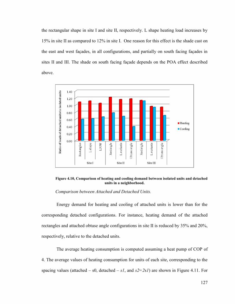
127
the rectangular shape in site I and site II, respectively. L shape heating load increases by
15% in site II as compared to 12% in site I. One reason for this effect is the shade cast on
the east and west façades, in all configurations, and partially on south facing façades in
sites II and III. The shade on south facing façade depends on the POA effect described
above.
Figure 4.10, Comparison of heating and cooling demand between isolated units and detached
units in a neighborhood.
Comparison between Attached and Detached Units.
Energy demand for heating and cooling of attached units is lower than for the
corresponding detached configurations. For instance, heating demand of the attached
rectangles and attached obtuse angle configurations in site II is reduced by 35% and 20%,
respectively, relative to the detached units.
The average heating consumption is computed assuming a heat pump of COP of
4. The average values of heating consumption for units of each site, corresponding to the
spacing values (attached – s0, detached – s1, and s2=2s1) are shown in Figure 4.11. For

128
site I, only configurations of the rectangular shapes and of L variants are shown in Figure
4.11, since obtuse angle is not applicable to this site.
Doubling the spacing of units (from s1 to s2=2s1), does not affect significantly
the heating energy consumption. While cooling energy consumption increases with larger
spacing between units, it should be noted that it is negligible compared to heating energy
consumption (ca. 10%).
Figure 4.11, Heating consumption at different spacing between units.
Row Effect
Solar potential
Solar Irradiation
The row effect on incident and transmitted radiation in site I is assessed by
comparison of the corresponding radiation levels on south façades of the obstructed row
with those of the unobstructed row. The results indicate that the distance between rows
A-s0

129
has a significant effect on solar radiation incident on the façades of the obstructed row.
For instance, for the smallest row spacing (r=5m) the transmitted radiation by the south
façade windows may be reduced by as much as 95% on the exposed branch façade of
attached L variant configuration (Fig. 4.12a), by 60% for the detached L variants and by
some 85% for the detached rectangular shapes. A similar effect is found for the incident
radiation.
At 20m, corresponding to a density of about 8 -10 u/a , the maximum effect is
about 13% reduction of incident and transmitted radiation on the attached L variant
configuration and 9% on the detached rectangle. At 20m, the row effect on the shaded
façades of L variant configurations is small, reaching a maximum reduction of about 6%
for WDD.
Figures 4.12a and 4.12b represent the results in term of the reduction of solar
radiation transmitted by the windows of the obstructed row as compared to the
corresponding unobstructed row, for some selected configurations. For non-convex
shapes (VWS30) the effect is given for the shaded and for the exposed façades.
(a)
South Shaded
Facade
South Facade

130
(b)
Figure 4.12, Reduction in transmitted radiation due to row effect for WDD. U1, U2 and U3
are the units of the shaded row (U2 is the middle unit): a) Effect on selected configurations at 5m row
separation; b) Effect on detached rectangular units, at separations of 5, 10 and 20 m.
Energy Generation
The row effect on electricity generation is measured by comparing the electricity
generation of the roofs of the obstructed rows to that of the exposed row. The results
show that for a row separation of 5 m the electricity generation of the rectangular unit is
reduced by a maximum (for the middle units) of 3% for the SDD and 7% for the WDD.
The row configuration has no significant effect on the south facing L shape (L-SW) and
L variant V-WS30 (β=30º), both attached and detached. North facing L shape (L-N)
performs in similar way to the rectangular shape. No shadowing effect on electricity
generation is observed for row separation larger than 5 m. The yearly generation of all
configurations is not significantly affected by the distance (<4%).
Energy Demand
The row effect on heating and cooling loads is assessed for site I by comparing
the loads of obstructed and obstructing rows to the corresponding isolated row. The
results for heating loads are presented in Fig. 4.13 for detached configurations and in Fig.

131
4.14 for attached configurations. Figures 4.13a and 4.14a show the heating loads of the
obstructing and obstructed row relative to the isolated row. Figs 4.13b and 4.14b present
the actual average heating loads. Results indicate that, generally, the average heating load
increases significantly for the units of the obstructed row (R2), while the cooling load
decreases. For the exposed row (R1), heating and cooling load are affected for a row
spacing of 10m or less. Following are the main observations:
The heating load of the obstructed row of detached rectangular units (Fig. 4.13)
increases by ca. 50% at 5m row spacing and by 25 % at 10m spacing. The
corresponding values for the exposed row are 15% and 5%, respectively.
For attached rectangular units (Fig. 4.14), the increase in the heating load of the
obstructed row is about 70% at 5m row spacing and 30% at 10m spacing. At 20
m there is no significant effect.
For detached L-S and L-N configurations, at 5m distance the obstructed row
requires around 40% more energy for heating than the isolated row (Fig. 4.13).
The effect on the obstructed row is not significant for a distance of 15m or more.
For the attached configurations, an effect of 50% is observed for a distance of 5m.
For a distance of 10m and more, heating load of the obstructed row is not
significantly affected by the obstructing row.
For L variant, the exposed row is not affected, while the obstructed row of
detached units requires 25% more heating at 5m spacing, and 10% at 10m. The
attached units of L variant in the obstructed row require 35% more heating at 5m,
and 15% at 10m spacing.

132
(a)
(b)
Figure 4.13, Detached units (a) Heating load of two rows relative to isolated rows, (b)
Heating load of the two rows of detached units.
V-WS30
Hea
tin
g l
oad
(kW
)

133
(a)
(b)
Figure 4.14, Comparison of the row effect in site I ‒ R1 exposed row, R2 obstructed row: (a)
Comparison to isolated row, (b) Heating loads of the two rows.
Fig. 4.15 presents the ratio of heating load of the obstructed to isolated row, for
detached rectangular shape, expressed as function of the distance between rows. This
distance is presented as percentage of the minimum distance between rows to avoid
shading (x = 25 m, see above). The decrease in heating load has a quadratic correlation
with the distance between the rows, as shown in Figure 4.15.
Hea
tin
g l
oad
(kW
)

134
Figure 4.15, Ratio of heating load of the obstructed row to the unobstructed row as function
of the minimal distance required to avoid shading
4.2.3. Effect of Site Layout
This section investigates the effects of site layout on the solar potential and
energy performance of neighborhoods. Site I with east-west (E-W) oriented road serves
as reference for assessing the effects of different site layouts on the response variables of
housing unit configurations that are common to these layouts. Additional effects are
studied for site specific configurations that are not shared by the reference site. The
detailed analysis is presented below.
Straight Road - Effect of Road Orientation
The effect is studied only for detached units (Fig. 4.3). The main site effect
comparison is between inclined roads and the E-W road which is the reference. Effects
on individual units are assessed by comparison is to isolated units of the same shape and
orientation.

135
Solar Potential
Solar Radiation
The effect of road orientation on solar radiation on façades of units along the road
is influenced by the orientation of the units and their façades, as well as by shading due to
POA and the distance between the units. To assess the effect of variations of road
orientation on the incident solar radiation, units in different configurations are compared
to the corresponding isolated units, of the same orientation. The effect of orientation on
solar radiation is studied in Chapter III (section 3.2.3).
The effect on L variant configurations is as follows: The yearly solar radiation on
the shaded façade of LVW60 (+60o road) is reduced by up to 15%, and by about 30% for
the WDD, as compared to the isolated unit. For LVW45 (+45o road) the yearly reduction
is about 10%.
The solar radiation incident on the south facing rectangular shape is reduced by a
maximum of 9%, due shade cast by adjacent units. For the configurations where the
whole rectangular unit is oriented toward the street, there is no shading effect and the
radiation on the façade changes according to the orientation of the isolated unit, as
indicated in Chapter III (a reduction of about 20% for 30° and up to 60% for an
orientation of 60° on a WDD).
Energy Generation
The effect of road orientation on the average electricity generation is evaluated by
comparing the annual energy yield of each of the studied configuration with its
counterpart in the E-W road layout. Thus, the rectangular configurations in each inclined
136
road configuration are compared to the rectangular configuration of E-W road. Since the
only L variant studied in the E-W road of site I is LVW30, the corresponding L variations
configuration in the inclined road (+30o) is analyzed (Fig. 4.3).
No significant effect is found in the case of the south facing rectangles or L
variants. In configurations where rectangular units are oriented to face the road,
electricity generation is only affected by the orientation, since mutual shading has no
effect. Detailed study of the effect of orientation on electricity generation is presented in
Chapter V.
Energy Demand
The effect of road orientation on the energy demand for heating and cooling of
units is found by comparing the heating and cooling load of the units of rectangular and
V-WS30 configuration to the corresponding configuration in the E-W reference road.
Comparison to the isolated units is also given to allow for those configurations that are
not shared by the E-W road layout (such as non-south-facing rectangles and L variants
with wing rotation other than 30o). The main observations are summarized in the
following:
The energy demand for heating of the rectangular south facing configurations (R)
is not significantly affected by the road inclination (maximum of 9% increase).
However the use of land is increased significantly (by up to 29%) as compared to
the south facing rectangles of E-W road.
Rectangular configurations that are oriented (R (O)) towards the road use less
land than all other configurations. However, they require significantly larger

137
heating energy (up to 36%) as compared to the south facing rectangular E-W road
configuration.
V-WS60 requires up to 29 % more energy than the isolated units. V-WS60 has an
increased energy demand primarily because of the relative position of the units,
where a large portion of the south facing façade is shaded. This effect can be
reduced by increasing the distance between units. However, increasing the
distance can lead to an increase of land use area.
Figure 4.16 and Table 4.6 present results for positive rotations of road orientations
(General SE-NW orientation). Configurations with negative rotation show similar
results with a difference of 2-3% in loads (requiring less energy).
Figure 4.16, Comparisons of heating/ cooling loads and land use area of all configurations
(R-south facing rectangles; (R-O) rotated rectangles and V shapes), of the inclined road sites.
0
50
100
150
200
250
300
0
500
1000
1500
2000
2500
3000
3500
4000
Are
a (m
2)
Load
(kW
)
Average Heating
Average Cooling
Total Area of land

138
Table 4.6, Summary of the results analysis of the inclined road configurations
Configurations
Average
Heating
load (kW)
Average
Cooling
load (kW)
Land
area per
house
(m2)
Comparison of
heating load to
configuration
of E-W
Compariso
n to
isolated
units
Ratio of land
area to
reference
case (E-W)
Road +30°
R 2638.20 180.72 266.67 1.00 1.05 1.21
R(O-30) 2967.01 229.21 227.67 1.13 1.18 1.03
V-WS30 3065.69 189.56 237.67 1.15 1.14 1.08
Road +45°
R 2650.72 198.50 283.33 1.01 1.06 1.29
R(O-45) 3312.84 269.76 227.67 1.26 1.32 1.03
V-WS45 3052.00 249.81 245.33 - 1.13 1.12
Road +60°
R 2730.73 190.08 268.67 1.04 1.09 1.22
R(O-60) 3573.96 318.18 227.67 1.36 1.42 1.03
V-WS60 3439.43 300.80 250.00 - 1.29 1.14
Curved Road
As mentioned above, the effects of density and site layout are strongly coupled for
curved layouts. The main comparison for overall site effect is between sites with curved
road (II and III) and site I (with E-W road). This comparison can only be applied to
configurations of similar unit shapes and density. The effect of curvature on solar
performance of individual (detached) units of a given shape in the neighborhood can be
assessed by reference to the isolated, south oriented unit of the same shape.
Solar Potential
Solar Radiation
The incident radiation on the near south façades of individual units and
transmitted by their windows, in each detached assemblage is compared to isolated south
facing units to assess the effect of shade from adjacent units. In attached configurations
comparison is carried out with respect to the corresponding detached units of the same
configuration, to assess the effect of density.

139
The rectangular units of site I are positioned in straight layout facing south and
therefore the south facing façades of detached units are not affected by adjacent units.
For detached L and L variants in site II and III, the main effect, as compared with site I, is
due to the rotation of units relative to the south, along the curved layout. In addition,
some units in these configurations cast shadows on façades of adjacent units. The WDD
reduction of incident radiation on the south facing façades ranges from about 4% on the
central units, to up to 30% for some adjacent units (e.g. U2 and U4 in L variants,
Fig.4.4b), in comparison to the isolated south facing units. This depends on the distance
between the units, and on the POA value which determine the extent of shading.
For the attached configurations, the method of assemblage of L variant (Fig. 4.6)
results in self- shading geometries (non-convex configurations). In these cases the ratio of
the dimensions of mutually shading façades of adjoined units is of importance, and
should be taken into consideration in the design. The decrease of solar radiation, relative
to the corresponding detached unit, can reach up to 30%, in some of the studied cases,
depending on the ratio of the dimensions of mutually shading façades (similar to the
depth ratio effect of a non-convex shape, Chapter III).
Energy Generation
The site layouts are compared for the three configurations that are common to the
three sites. These configurations are detached rectangles, detached L variants, and
attached L variants. The performance of these configurations of sites II and III, is
compared to the performance of site I. The response variable for the comparison is
electricity generation per unit area averaged over all units in a neighborhood.

140
No significant effect of the site layout is indicated on overall electricity generation
per unit area. A maximum reduction of about 3% is observed in the generation of the
detached rectangle configuration in sites II and III as compared with the similar
configuration in site I. Comparing the annual energy generation of the total roof area, an
increase of 6% and 9% is observed, for the attached L variant configuration in site II and
site III respectively, as compared to the corresponding configuration in site I. The results
are presented in Table 4.7.
Table 4.7. Site layout effect on average electricity generation for summer and winter design
days (SDD and WDD), and annually
Shift of Peak Electricity Generation
An important result of the interaction of site layout and configurations is the shift
of peak electricity generation. This effect is mainly found in sites II and III, where
different shape orientations are dictated by the layout of the road.
A significant shift of the profile of the electricity generation is obtained by the
BIPV of different units. In site I the difference in timing of peak electricity is due, to the
rotation of the south wing of V shape. A maximum shift of 3 hours is obtained in site I. In
sites II and III an additional source is the rotation of whole units. A difference of peak
time of up to 6 hours is observed in the configurations of site II and site III.
Site Site II/site I Site III/site I
Design period SDD WDD Annual
Annual per
total area SDD WDD Annual
Annual per
total area
Detached
Rectangles 1.02 0.91 0.97 0.97 1.02 0.90 0.97 0.97
Detached L
variant 0.98 0.97 0.99 1.04 0.88 0.99 1.00 1.05
Attached L
variant 1.04 0.99 1.01 1.06 0.99 1.00 1.01 1.09

141
Figure 4.17 presents the daily variation of electricity generation of configurations
of site II for the winter design day. Electricity generation profiles for attached rectangular
(trapezoid) units are presented in Figure 4.17a. The graphs of Figure 4.17 b, c show the
electricity generation profiles of the hip roof of wings of units of detached and attached L
variant configurations of site II. It should be noted, however, that the hip constitutes a
small portion of the electricity generating roof surface and the overall effect on total
generation would be reduced.
(a)
(b)
0
0.5
1
1.5
2
2.5
3
5 10 15 20
kW
Time (hr)
U3
U4
U2
U5
U1
0
0.2
0.4
0.6
0.8
1
1.2
5 10 15 20
kW
Time (hr)
U1
U2
U4
U5
(
a)
(
b)
(
d)

142
(c)
Figure 4.17, Hourly electricity generation (from 4-6 AM to 6-8 PM) (kW) for site II, on a
WDD: a) on the total south roof of attached rectangular (trapezoid); b) on the hip of L variants of
detached L variants; c) on the hip of L variants of attached L variants.
Energy Demand
The effect of site layout on energy demand is analyzed by comparing
configurations of rectangular and L variant shapes in site II and site III to the
corresponding configurations in site I. The results are presented in Figure 4.18. For
detached configurations, only the cooling load increases in site II and III. For instance,
the cooling load of the rectangular configurations is increased by approximately 45% and
48% for site II and site III, respectively. However, the energy demand for cooling is low
relative to heating (<10%, for the rectangular configuration in site II). One important
reason for the increase of cooling load in sites II and III, particularly for rectangular units,
is the rotation of units around the curve towards east or west, resulting in increased
transmitted radiation in the morning and the evening, when the sun is at low altitude
during the summer period. This can be resolved by modifying the window area, for the
rotated units.
In attached configurations, the heating load of L variants in site III is 25% higher
than in site I. This can be explained by the shade cast on several south façades of this
0
0.2
0.4
0.6
0.8
1
5 10 15 20k
W
Time (hr)
U1
U4
U2
U3
U6
U5
(
f)
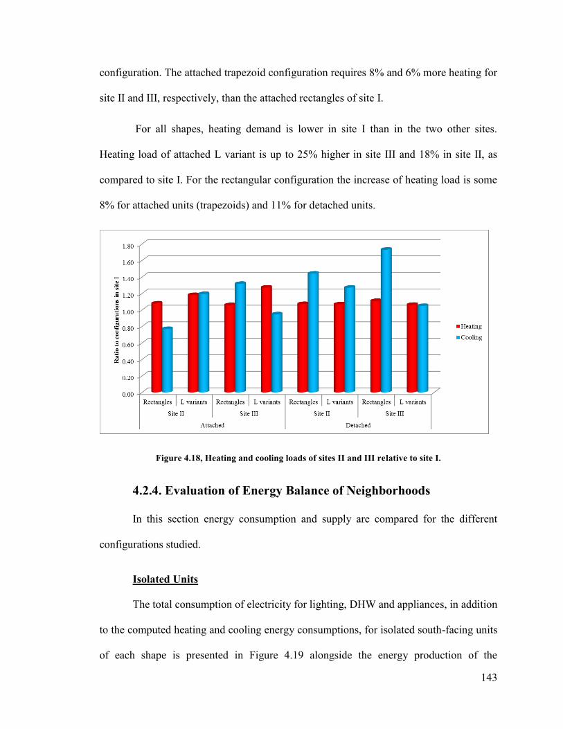
143
configuration. The attached trapezoid configuration requires 8% and 6% more heating for
site II and III, respectively, than the attached rectangles of site I.
For all shapes, heating demand is lower in site I than in the two other sites.
Heating load of attached L variant is up to 25% higher in site III and 18% in site II, as
compared to site I. For the rectangular configuration the increase of heating load is some
8% for attached units (trapezoids) and 11% for detached units.
Figure 4.18, Heating and cooling loads of sites II and III relative to site I.
4.2.4. Evaluation of Energy Balance of Neighborhoods
In this section energy consumption and supply are compared for the different
configurations studied.
Isolated Units
The total consumption of electricity for lighting, DHW and appliances, in addition
to the computed heating and cooling energy consumptions, for isolated south-facing units
of each shape is presented in Figure 4.19 alongside the energy production of the

144
corresponding units. The electricity production of the reference rectangular layout with
hip roof is some 35% less than consumption. Some L variants, such as V-EN30W,
produce up to 96% of total consumption. The results in terms of percentage of energy
production to energy consumption of all shapes are presented in Table 4.8.
(a)
(b)
Figure 4.19, Energy consumption and production for isolated units of different shapes: a)
Shapes of sites I and II; b) Shapes of site III.
a b E
ner
gy c
on
sum
pti
on a
nd g
ener
atio
n (
kW
h)
En
erg
y c
on
sum
pti
on a
nd g
ener
atio
n (
kW
h)
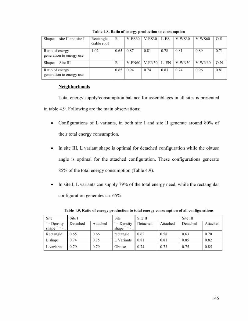
145
Table 4.8, Ratio of energy production to consumption
Shapes ‒ site II and site I Rectangle -
Gable roof
R V-ES60 V-ES30 L-ES V-WS30 V-WS60 O-S
Ratio of energy
generation to energy use
1.02 0.65 0.87 0.81 0.78 0.81 0.89 0.71
Shapes ‒ Site III R V-EN60 V-EN30 L–EN V-WN30 V-WN60 O-N
Ratio of energy
generation to energy use
0.65 0.94 0.74 0.83 0.74 0.96 0.81
Neighborhoods
Total energy supply/consumption balance for assemblages in all sites is presented
in table 4.9. Following are the main observations:
Configurations of L variants, in both site I and site II generate around 80% of
their total energy consumption.
In site III, L variant shape is optimal for detached configuration while the obtuse
angle is optimal for the attached configuration. These configurations generate
85% of the total energy consumption (Table 4.9).
In site I, L variants can supply 79% of the total energy need, while the rectangular
configuration generates ca. 65%.
Table 4.9, Ratio of energy production to total energy consumption of all configurations
Site Site I Site Site II Site III
Density
shape
Detached Attached Density
shape
Detached Attached Detached Attached
Rectangle 0.65 0.66 rectangle 0.62 0.58 0.63 0.70
L shape 0.74 0.75 L Variants 0.81 0.81 0.85 0.82
L variants 0.79 0.79 Obtuse 0.74 0.73 0.75 0.85

146
Chapter V: Roofs3
This chapter presents an in-depth study of roofs for increased solar potential. The
basic principle is the utilization of complete near-south facing roof surfaces for solar
collectors that generate both heat and electricity through the application of a building-
integrated photovoltaic/thermal (BIPV/T) system. An open loop air-based BIPV/T system
is assumed in this study. Following is a brief outline of the chapter’s contents.
Section 5.1 presents the principles of the open loop air based BIPV/T system, as
well as the numerical model employed to obtain a correlation between thermal and
electrical output of the system. Section 5.2 investigates the effect of combinations of tilt
and orientation angles of a roof surface on the BIPV/T output. Section 5.3 presents design
alternatives for the roof of a building of rectangular layout, starting with a simple hip roof
design and advancing to more complex multi-surface configurations, aimed at optimizing
energy production. Values of the design parameters investigated are presented in terms of
the tilt and orientation angles of the various surfaces. An option of redesigning the basic
rectangular shape to follow the contour of multi-surface roof geometries is also
investigated.
Simulation results and their analysis are presented in section 5.4. The analysis
relates to energy production, including both electricity and useful heat collection. The
effect of roof design on energy demand, in terms of heating and cooling loads, is also
investigated. This analysis is performed for all roof configurations, as well as for
3 The study and some of the results presented in this chapter are published in:
Hachem C., A. Athienitis, P. Fazio, (2012b). Design of roofs for increased solar potential of BIPV/T
systems and their applications to housing units", ASHRAE Transactions, TRNS-00226-2011.R1.

147
redesigned layout to fit multi-surface roofs. A rectangular unit with hip roof (45° side and
tilt angles) serves as reference for comparing design alternatives. Overall energy
performance is assessed in terms of annual electricity generation versus total energy
consumption for all roof variants.
5.1. BIPV/T system
This section presents the numerical model employed to obtain a correlation
between thermal and electrical efficiency of the open loop air based BIPV/T system. The
air circulated behind the PV panels assists in cooling these panels, increasing thus their
electrical efficiency, and in recovering heat that can be used for space or/and water
heating. The useful fraction of thermal energy generation depends on the temperature of
the solar heated air and on the end uses. For instance, a BIPV/T system coupled with a
heat pump enables exploiting low temperature outlet air to offset heating load or for
direct space heating, while higher outlet air temperature can be employed to heat
domestic hot water or sent to storage.
Approximate Model
A transient quasi-two-dimensional finite difference model is employed to
determine the thermal energy generation potential of the BIPV/T system, and to establish
a relationship between electricity and useful heat generation. A gable roof of the
rectangular unit, with a tilt angle of 45° is employed in the model. The model is applied
to the design days as well as to selected sunny days representing each month of the year.
The model is applied to roofs with different tilt angles, ranging from 30° to 60°, at 5
degrees increments. Environmental parameters including outside temperature, solar

148
radiation, wind speed and sky temperature are provided by the weather data files of
EnergyPlus.
The BIPV/T system, illustrated in Fig. 5.1a, is divided into five control volumes
along the direction of the ridge. Figure 5.1b depicts the thermal network of one control
volume of the BIPV/T system. The various thermal conductance coefficients, including
that associated with the air flow (MCair), are presented in Figure 5.1b. The PV panels are
assumed to have negligible thermal resistance and thermal capacity (Liao et al, 2007).
The bottom surface of the air cavity is assumed to be well insulated.
(b)
Air inlet
Insulation
(a)
BIPV
Air cavity
Hot air
flow
Solar radiation
(a)
(a) Tair
(i)
To Qe(i) Qsky(i)
Qs(i)
hr hc
Insulatio
n Qu(i) hc
TPV(i)
Tb(i)
Air flow
MCair Node (i)

149
Figure 5.1, a) Cross-section illustrating an open loop BIPV/T system , b) schematic
illustrating the thermal network in one control volume of the BIPV/T system (refer to eqs. 5.1-5.8 for
meanings of symbols).
The governing equation describing the explicit finite difference method for a
thermal network, corresponding to a node i and time interval p, is expressed by Athienitis
(1998):
∑
∑ (eq. 5.1)
where T is the temperature of a node at a specific time, qi is the heat source at the
node in question, j is an adjacent node, U(i, j) is the heat transfer coefficient between
nodes i and j, and p indicates the present time step.
The total electrical energy is determined as function of the efficiency and the solar
radiation as follows:
𝜂 (eq. 5.2)
where (𝜂PV) is the PV efficiency (Eq. 5.3), A is the surface area of the roof and G
is the solar radiation (W/m2). The electrical efficiency of the BIPV (𝜂PV) system is
computed by the following linear equation (Skoplaki and Palyvos, 2009; Whitaker et al.,
1991):
𝜂 𝜂 { ( )}
(eq. 5.3)
where 𝜂STC is the efficiency of the PV cells under standard test conditions (STC),
β is the PV module temperature coefficient, and TSTC is the standard test condition
temperature (25ºC). A value of 12.5% is assumed for 𝜂STC.

150
The total thermal energy generated by the BIPV/T (Qu) can be expressed as
follows:
𝜂 (eq. 5.4)
Qu is determined as function of the inlet air temperature entering the BIPV/T
system, assumed as the outside air temperature (To), and the outelt air tempurature of the
system (Toutlet-BIPV/T) (outlet air of the last control volume), (Athienitis et al., 2011):
(eq. 5.5)
The outlet air temperature at each control volume is determined as:
(eq. 5.6)
where Tin (i) is the inlet air temperature at each control volume, M is the mass
flow rate of air, Cair is the specific heat of air , and Qu (i) is the heat carried by the air
flow and is determined by the finite explicit model at each control volume as:
(eq. 5.7)
where As is the area of each BIPV/T section, hc is the convective heat transfer
coefficient in the cavity, Tpv is the temperature of the PV panel, Tb is the temperature at
the bottom side of the cavity, and (Tair) is the air temperature, computed in each control
volume by means of equation 5.8 (Charron and Athienitis, 2006).
(
)
(eq. 5.8)
where x is the length of the studied section, and
(eq. 5.9)
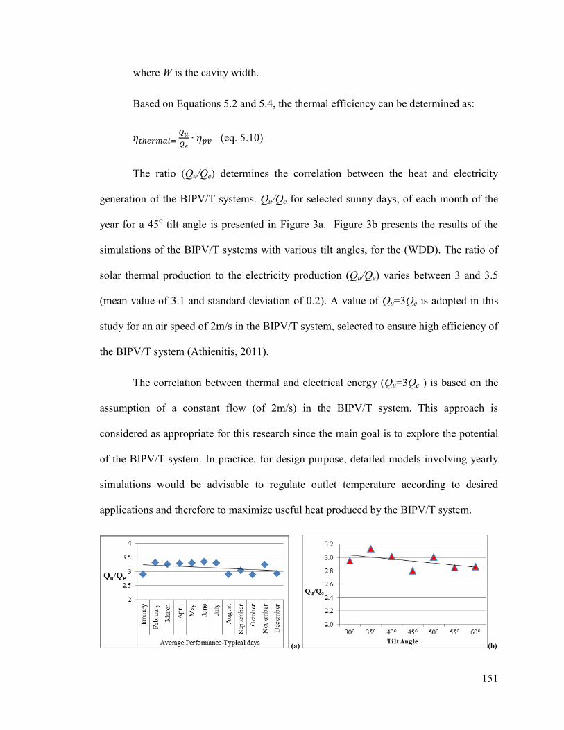
151
where W is the cavity width.
Based on Equations 5.2 and 5.4, the thermal efficiency can be determined as:
𝜂
𝜂 (eq. 5.10)
The ratio (Qu/Qe) determines the correlation between the heat and electricity
generation of the BIPV/T systems. Qu/Qe for selected sunny days, of each month of the
year for a 45o tilt angle is presented in Figure 3a. Figure 3b presents the results of the
simulations of the BIPV/T systems with various tilt angles, for the (WDD). The ratio of
solar thermal production to the electricity production (Qu/Qe) varies between 3 and 3.5
(mean value of 3.1 and standard deviation of 0.2). A value of Qu=3Qe is adopted in this
study for an air speed of 2m/s in the BIPV/T system, selected to ensure high efficiency of
the BIPV/T system (Athienitis, 2011).
The correlation between thermal and electrical energy (Qu=3Qe ) is based on the
assumption of a constant flow (of 2m/s) in the BIPV/T system. This approach is
considered as appropriate for this research since the main goal is to explore the potential
of the BIPV/T system. In practice, for design purpose, detailed models involving yearly
simulations would be advisable to regulate outlet temperature according to desired
applications and therefore to maximize useful heat produced by the BIPV/T system.
(a) (b)

152
Figure 5.2, a) Qu/Qe for 45o tilt angle roof for one sunny day of each month, over a year; b)
Qu/Qe for WDD of roofs with different tilt angles.
The correlation between thermal and electrical energy genration is employed to
determine the thermal energy as well as the outlet air temperature of BIPV/T systems of
different complex roof designs developed in this study.
Variable speed fan enables controlling the outlet air temperature, which can be
used for different purposes. Figure 5.3 presents the relation between air velocity and the
average air change temperature (ΔT- the difference between inlet and outlet air
temperature of the BIPV/T system), over the winter design day, in the BIPV/T system.
This relation is determined for the gable roof of the rectangular shape.
The inlet air temperature is the outside temperature obtained from EnergyPlus
weather data. The outlet air temperature decreases exponentially with increasing flow
rate, and vice versa. Flow rate and outlet air temperature should be determined to fit the
intended application. For instance, for heat pump lower outlet air temperature can be
used, while for space heating and hot water higher temperature is needed.
Figure 5.3, Relation beteen air velocity and the average air change temperature in the cavity
(ΔT), on a WDD.
0
2
4
6
8
10
12
14
16
0 0.5 1 1.5 2 2.5 3 3.5
Air
Tem
pera
ture (
°C)
Air Velocity (m/s)
Average air temperature change (∆T)

153
5.2. Basic Surface Parameters and their Effect
This section investigates the effect of roof surface parameters – tilt angle and
orientation relative to south ‒ on the energy performance of the BIPV/T system per m2 of
surface. The main response variables in assessing performance are the annual electricity
generation, the heat production during a heating period, assumed from October 15 to
April 15, and the total combined energy production.
5.2.1. Effect of Tilt Angle
The annual electricity generation of the BIPV/T system is not significantly
affected by a tilt angle that ranges between 30° and 50°. For a 60° tilt angle, the annual
electricity production is reduced by some 7% as compared to 45° tilt angle, while the heat
generation for the assumed heating period is reduced by only 2%. This is mainly due to
larger tilt angle having advantage in the winter months. For instance, the electricity
generation of the BIPV/T system with 60° tilt angle is reduced by 16% in June, as
compared to the system with 45° tilt angle, while the maximum monthly increase of
generation in December is about 6%. Figure 5.2 presents the average monthly electricity
production of various tilt angles.
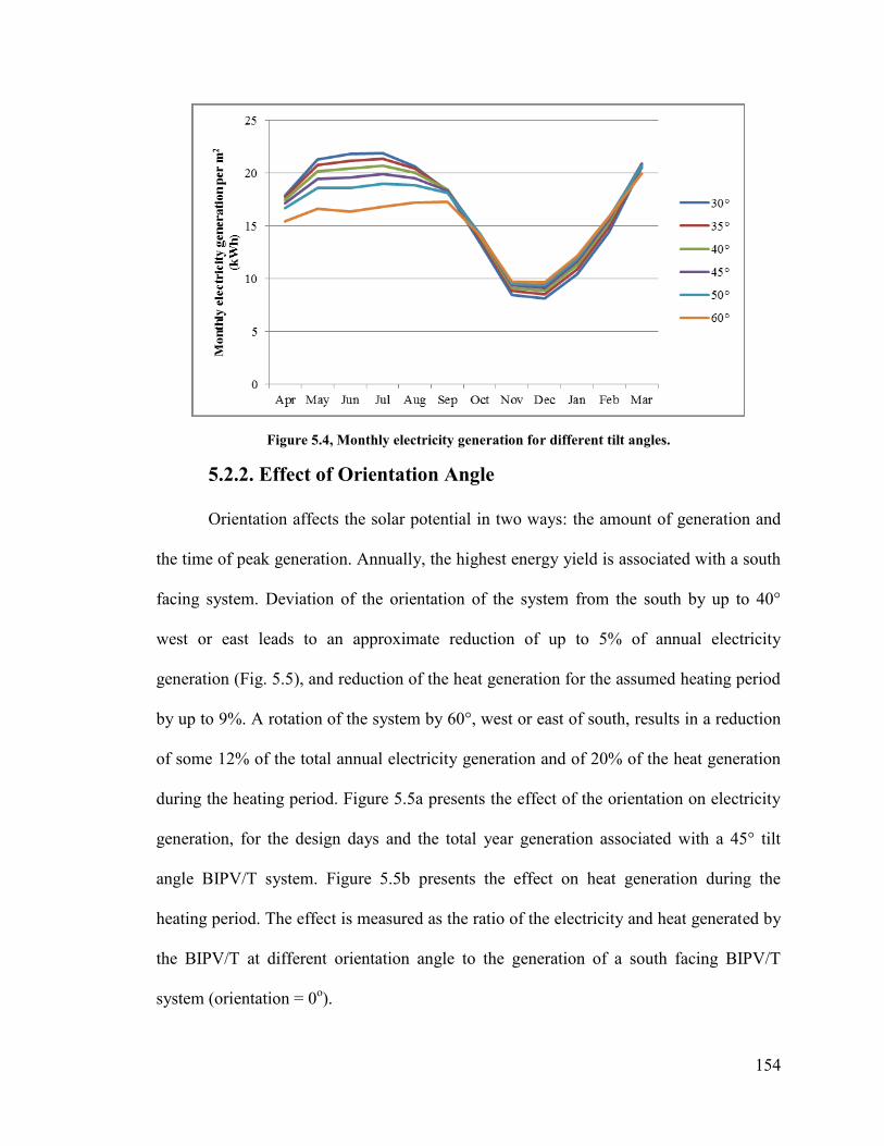
154
Figure 5.4, Monthly electricity generation for different tilt angles.
5.2.2. Effect of Orientation Angle
Orientation affects the solar potential in two ways: the amount of generation and
the time of peak generation. Annually, the highest energy yield is associated with a south
facing system. Deviation of the orientation of the system from the south by up to 40°
west or east leads to an approximate reduction of up to 5% of annual electricity
generation (Fig. 5.5), and reduction of the heat generation for the assumed heating period
by up to 9%. A rotation of the system by 60°, west or east of south, results in a reduction
of some 12% of the total annual electricity generation and of 20% of the heat generation
during the heating period. Figure 5.5a presents the effect of the orientation on electricity
generation, for the design days and the total year generation associated with a 45° tilt
angle BIPV/T system. Figure 5.5b presents the effect on heat generation during the
heating period. The effect is measured as the ratio of the electricity and heat generated by
the BIPV/T at different orientation angle to the generation of a south facing BIPV/T
system (orientation = 0o).

155
(a)
(b)
Figure 5.5, Effect of the angle of orientation on: (a) the electricity generation, (b) heat
generation over the period between mid-October and mid-April.
Monthly generation indicates that in the summer months, orientation of the
BIPV/T system towards west or east results in electricity generation that is close or
slightly higher than south orientation. Figure 5.6 presents the effect of orientation on
monthly electricity generation.
The orientation of the BIPV/T system affects not only the value of the electricity
generation, but also the time of peak generation. For a south facing system, the peak
generation is at solar noon. Rotation of the BIPV/T system towards the west results in
shifting the peak radiation to the afternoon and vice versa for east rotation. A 30°
orientation (east or west), enables a shift of peak generation time to up to 2 hours relative
to solar noon. An orientation of 60°-70° enables a 3 hours shift of peak. Roofs that
Orientation from south
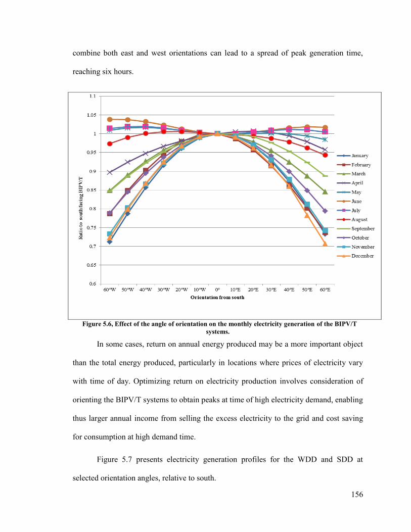
156
combine both east and west orientations can lead to a spread of peak generation time,
reaching six hours.
Figure 5.6, Effect of the angle of orientation on the monthly electricity generation of the BIPV/T
systems.
In some cases, return on annual energy produced may be a more important object
than the total energy produced, particularly in locations where prices of electricity vary
with time of day. Optimizing return on electricity production involves consideration of
orienting the BIPV/T systems to obtain peaks at time of high electricity demand, enabling
thus larger annual income from selling the excess electricity to the grid and cost saving
for consumption at high demand time.
Figure 5.7 presents electricity generation profiles for the WDD and SDD at
selected orientation angles, relative to south.

157
(a) (b)
(c) (d)
Figure 5.7, Effect of the angle of orientation on the electricity generation, (a) 30° for the
WDD, (b) 60° for the WDD, (c) 30° for the SDD, (d) 60° for the SDD.
5.2.3. Combination of Tilt and Orientation Angles
The yearly study shows that for the winter months between September and
March, the most effective BIPV/T systems are those that combine a tilt angle of 45° to
60° together with a south facing orientation. These configurations allow the highest yield
of electricity generation as well as heating energy. In the summer months, lower tilt
angles and rotation, particularly west, are advantageous.
Table 5.1 presents the annual electricity generation, the heat generation for the
heating period and the combined energy generation, for different combinations of tilt and
orientation angles.

158
Table 5.1, Electricity generation, heat generation and combined generation of various
combinations
Figure 5.8 presents the comparison of the results of all these combinations to a
south facing BIPV/T system with 45° tilt angle.
Figure 5.8, Ratio of energy generation of different configurations to south facing BIPV/T
system with 45° tilt angle.
5.3. Design of Roofs
This part of the study, explores various design possibilities of roof shapes for a
rectangular house, to maximize solar energy potential. The design proposed in this study
is conceptual; technical considerations relating to PV technologies are not addressed. The
Ori
enta
tio
n
Tilt
30° 45° 60°
Yearly
electricity
Generation
(kWh)
Heat
generation
(heating
Period)
(kWh)
Combined
generation
(kWh)
Yearly
electricity
generation
(kWh)
Heat
generation
(heating
Period)
(kWh)
Combined
generation
(kWh)
Yearly
electricity
generation
(kWh)
Heat
generation
(heating
Period)
(kWh)
Combined
generation
(kWh)
South 197 292 490 195 303 499 176 280 456
30W 193 281 473 189 288 477 181 297 478
30E 192 281 474 189 289 478 176 279 455
60W 179 250 429 173 248 421 159 234 394
60E 178 251 430 173 248 421 159 236 395

159
photovoltaic system is assumed to cover the total area of all south and near-south facing
roof surfaces. In practice, a small percentage of the roof area is used for the mounting
structure, for framing and for other technical considerations. It is further assumed that,
given the dynamic nature of current PV technology development, any future technology
will be capable of accommodating any specific requirements raised by the proposed roof
designs, such as PV modules of varying shape and size as well as inverters for different
BIPV/T orientations.
Three basic geometries of roofs are studied. The first geometry is a commonly
applied hip roof with varying tilt and side angles (Fig. 5.9). This Basic roof is applied to
all housing shapes. The second and third types of roofs are designed relatively
independently of the shape of the house, employing a multi-faceted roof surface
combining a range of tilt and orientation angles.
5.3.1. Hip Roofs
The basic roof design considered in Chapters III and IV is the hip roof with tilt
and side angles of 45° (see Fig. 5.9). Variations of this roof type, obtained by different tilt
and side angles are explored in this section for the basic shapes (Fig. 3.1) - square,
rectangle (aspect ratio 1.3), trapezoid (with aspect ratio of 1.3 and θ=60°), L (depth ratio
1), T, U, and H shapes. The tilt/side angle combinations studied are: 45°/45°; 45°/60°;
30°/45° and 30°/60°. L and T shapes have gable ends for the main wings (where side
angle is 90°).
An additional roof, termed hereunder the optimum roof, is designed to serve as
reference for comparative evaluation of the electricity generation potential by the BIPV/T

160
systems of all other roofs. The optimum roof is a gable roof with 45o tilt angle covering
the rectangular shape with aspect ratio of 1.3.
Figure 5.9, Illustration of hip roofs of basic shapes.
5.3.2. Advanced Roof Design
This section presents an advanced roof system design, which combines surfaces
of various tilt and orientation angles. The main goal of these roofs is to offer design
options that increase the solar potential of the BIPV/T systems. Orientation and tilt angles
that are optimal for the summer and winter months are selected and combined in such
roof systems. These advanced roof systems are applied to rectangular shapes. Some
additional studies that apply such roof concepts to L shape and L variants are included in
Appendix B. This extension of the concept, which is beyond the scope of this research,
can result in a large variety of roof shapes and possibilities that can be explored in future
investigation.
BIPV/T
Side
Angle

161
Split-surface Roof
The south-facing portion of the roof is divided into three plates of differing
orientations and tilt angles. A BIPV/T system is assumed to cover the total area of each
of these plates.
Two variants are considered, as well as some variations of these options. The mid
plate is south oriented while the side plates are rotated by equal angles, the east plate
towards the east and the west plate towards the west. In the first option, the orientation
angle of the side plates is 15°, while in the second option this angle is 30°.
For each of the two orientations, the effect on the overall solar potential of the
roof is assessed for a number of tilt angles . The two configurations of the split-surface
roofs are presented in Figure 5.10 and details of the combinations are included in Table
5.2.
Although the study assumes availability of suitable technology to cover the full
surface, investigation of employing PV strips of currently available systems, results in a
maximum loss of 4% of the total area.

162
Figure 5.10, Split-surface roof designs: (a) configuration 1, side plates with 15° orientation from
south; (b) configuration 2, side plates with 30° orientation from south.
Folded plate
Folded plate roof design refers in this thesis to the shape of the roof, not
necessarily to the structural system. The folded plate roof geometry is composed of
triangular plates with various orientations. Two basic shapes are designed. The first
configuration is composed of four plates, with the two side plates facing south (Fig.
5.11a). The second basic shape consists of three plates with the central plate facing south.
Figure 5.11c shows a variation of this shape composed of two basic units.
More complex designs can be derived by joining together two or more units of the
basic shape. Figure 5.11 presents the three configurations analyzed in this study. The first
configuration (Fig. 5.11a) is the 4-plate basic shape, with the central plates rotated 15o
east and west and the side plates having 45° tilt angle. The second configuration (Fig.
5.11b) is composed of two basic 4-plate units, with central plates rotated 30° east and
west. The third configuration (Fig. 5.11c) is composed of two three-plate basic shapes
with side-plates rotated 30o east and west. It should be noted that the configurations of
(a) (b)
15° 30
°
Side plates
Central
plate
BIPV/T
15° 30°
A
A
B C D
C
S
B
D
Orientation
angle
Different tilt
angles
B
D

163
Fig. 5.11 maintain the same geometry on the north side. In practice, there is no need to
shape the roof symmetrically since it can add to the cost. Details of the folded plates’
configurations are presented in Table 5.2.
Figure 5.11, Folded plate roof designs, (a) configuration 1 ‒ basic 4-plate with 15° orientation
of the central plates; (b) Configuration 2 ‒ two basic 4-plate units with 30° orientation, (c)
Configuration 3 – two basic 3-plate roof with 30° orientation.
Table 5.2, Design Consideration Split- Roofs and Folded Plates’ Roofs
Complex
roof
Side
angle
Number of
surfaces
Combinations of orientation and tilt of the plates
(The first number refers to the orientation and the second to the tilt angle)
split-
surface
roofs
90° 3 Configuration 1 Center plate 0°, 45°; 0°, 50°; 0°, 45°;
Side plates 15°(E,W),
40°
15° (E,W), 40° 15° (E,W),
30°
Configuration 2 Center plate 0°, 45°; 0°, 50°; 0°, 45°;
Side plates 30°(E,W),
40°
30° (E,W), 40° 30° (E,W),
30°
Folded
plate
90° 4 (Basic 4-
plate)
Configuration 1 Center plates 15° (E, W)
Side plates 0°, 45°;
7 (2 basic 4-
plates)
Configuration 2 Center + end
plates
0°, 45°;
Side plates 30° (E, W)
6 (two 3-plate
basic shapes)
Configuration 2 Center plates 0°, 45°;
Side plates 30° (E, W)
(c) (b) (a)
15°E 30°E 30°W
15°W 30°E 30°W
Central
plates
4- folded plate basic unit
3- folded plate basic unit

164
5. 3.3 Redesign of Units
Configurations that involve surfaces of varying orientations (such as split-surface
and folded plates) may result in large overhangs. Modification of the south façade to
follow the roof outline can be applied to avoid such overhangs. In this section the
rectangular shape of the housing unit is re-designed to fit the outline of the multi-faceted
roof. The floor area is maintained fixed. The objective of this section is to assess the
effect of the design change on energy demand for heating and cooling.
In the split-surface option the south façade is split into three surfaces that are
oriented according to the associated roof portions. Figure 5.12 shows the rectangular
shape in its original form and the redesign associated with the split-surface option of
configuration 1 (Table 5.2. Configuration 2 is similar in shape).
Figure 5.12, Split- roof option with: (a) rectangular shape, (b) redesigned south facing
façade.
Redesign of the south façade of the folded plate roof options follows the same
principle. In configuration 1 (basic 4 folded plates, Table 5.4). The result is a two-surface
façade of a convex shape (Fig. 5.13a). Redesign for the second and third configurations
(a) (b)

165
(Fig. 8b and c, Table 5.4) leads to a non-convex saw-tooth shape of the south façade, in
order to conform to the roof outline (Fig. 5.13b).
Figure 5.13, Folded plates roof option with: (a) rectangular shape, (b) redesigned south
facing façade.
Complex roof surfaces with associated compatible facades such as saw-tooth may
be more applicable to projects of larger size than single family housing units, such as
large residential developments (for instance multiplexes) or commercial buildings, which
are more conducive to increasing architectural complexity.
5.4 Presentation and Analysis of Results
5.4.1. Roof Morphology Effect
The effect of roof morphology on its thermal/electrical potential is assessed by
comparing the electricity and heat generation of each roof design to those of the reference
case and the optimal roof (rectangular gable roof with tilt angle of 45°, Table 5.3).
Simulations using EnergyPlus were performed to determine the energy generation
potential of all roof shapes presented in section 5.3. The thermal generation of the
BIPV/T system, for a constant air flow of 2m/s, is assumed to constitute 3 times the
(a) (b)

166
amount of electricity generation for a given period (based on an approximate model, see
section 5.1 above). Results are presented for the annual electricity generation and for the
winter and summer design days. Heat generation results are over the assumed heating
period (mid-October to mid-April) and for the winter design day. The combined annual
electricity and winter heating energy production is also presented. The main observations
drawn from the analysis of all roof designs are summarized below.
It should be noted that heat generation can be employed for water heating and for
various appliances, resulting in an increase of the overall potential use of the output of the
BIPV/T system year round.
Hip Roofs
Table 5.3 presents the comparison of all studied configurations to the optimum
roof (rectangular layout with gable roof), expressed as the ratio of annual electricity
generation of each roof to that of the optimal roof. Annual energy generation and heat
generation during the heating period are presented in Table 5.4, for all hip roof options.
Figures 5.14 and 5.15 illustrate the annual generation and the peak electricity generation,
respectively, for the design days for all variants. The main observations are highlighted as
follows.
With a tilt angle of 30º, the peak generation on the SDD is slightly lower than on
the WDD (Figure 5.15a). However, with tilt angle of 45º, the peak generation is
significantly larger for a WDD (Figure 5.15b).This is mainly due to the fact that a
tilt angle of 45° is more advantageous for the winter solar radiation incident angle
than for the summer radiation.

167
In general, electricity generation is proportional to roof surface area. Given a
fixed floor area, roof surface area can be manipulated through various design
strategies such as:
o Combination of side angle and tilt angle. For instance, a rectangular layout
with side angle of 45º and tilt angle of 30º possesses a larger south-facing
surface area than with a tilt angle of 45º. Consequently the yearly
electricity generation is larger with the 30o tilt, even though a tilt angle of
45º allows higher radiation per unit area (5.67kWh/m2, as against
4.86kWh/m2
for 30º tilt angle, for the WDD).
o The largest south roof area is obtained with large side angle (60°for all
shapes). The optimal roof, having a side angle of 90° corresponding to a
gable roof. The electricity and heat generation of a hip roof with a 45° side
angle is reduced by approximately 40% as compared to the gable roof.
o The effect of different designs of hip roof (changing the magnitude of side
angle) on the heating and cooling loads is not significant (5% or less). For
instance, the heating load required for the housing unit with gable roof is
approximately 5% larger than for the unit with hip roof of 45° side angle
(reference case).
Table 5.3, Ratio of annual electricity generation of different variants of roofs, to the optimum roof
(gable roof)
Optimum
roof -
Gable
roof
Total Area
of PV
covered
surface
(m2)
40
Electricity
generated
per WDD
(kWh)
26.48
Peak
electricity
generated -
WDD (kW)
4.32
Electricity
generated
per SDD
(kWh)
34.81
Peak
electricity
generated
-SDD
(kW)
4.33
Annual
electricity
(MWh)
7.85
Tilt-Side angles
Ratio of annual electricity generation to gable roof for different shapes
Square Rectangle Trapezoid L shape U shape H shape T shape
1) 45-45 º 0.53 0.62 0.85 0.63 0.60 0.77 0.90
2) 45-60 º 0.75 0.81 1.10 0.58 0.76 0.97 0.86
3) 30-45 º 0.61 0.66 0.88 0.47 0.64 0.77 0.70
4) 30-60 º 0.73 0.75 0.95 0.44 0.73 0.86 0.66

168
Table 5.4, Yearly energy and heat generation of all hip roof options
Shape
Hip roofs
45°-45° 45°-60° 30°-45° 30°-60°
Electricity generation
(kWh/yr)
Heat
generation
(heating period)
kWh/yr
Electricity generation
kWh/yr
Heat
generation
(heating period)
(kWh/yr)
Electricity generation
(kWh/yr)
Heat
generation
(heating period)
(kWh/yr)
Electricity generation
(kWh/yr)
Heat
generation
(heating period)
(kWh/yr)
Square 4233 5588 5671 7485 4612 6088 5520 7286
Rectangle 4867 6451 6124 8084 4990 6587 5671 7485
Trapezoid 6777 8945 8317 10979 6654 8783 7183 9481
L shape 4948 6544 4385 5789 3554 4691 3327 4391
U shape 4835 6382 5746 7585 4839 6388 5519 7286
H shape 6168 8142 7334 9681 5822 7685 6502 8583
T shape 7228 9540 6502 8583 5293 6986 4990 6587
Figure 5.14, Annual electricity generation of roofs with differing tilt-side angles and shapes.
(a)

169
(b)
Figure 5.15, Peak electricity generations (kW): a) Tilt angle 30°; b) Tilt angle 45°.
Advanced Roof Designs
Split-surface Roofs
The split-surface roof design has two main characteristics: it enables larger south
facing roof area (about 48m2 as compared to 40m
2 for the gable roof) and it facilitates
combinations of orientation and tilt angles, which allows obtaining spread of peak
generation time of up to 3 hours (Fig.5.16).
The results (Table 5.6) indicate that there is no significant change of the energy
potential between the different combinations, of configuration 1 and 2 (3% or less). A
significant increase in the annual energy production is however obtained using this roof
design, as compared to the gable roof. For instance, configuration 1 (with 15° orientation)
exceeds annual electricity generation of the gable roof by 17% and heat generation for the
assumed heating period by 15%. Table 5.6 presents the annual electricity generation, the
heat generation for the heating period and the combined energy potential. The potential

170
heat generation on the WDD and the average air temperature difference (ΔT) are also
presented in Table 5.6.
(a) (b)
Figure 5.16, Electricity generation on design days for the plates of the 30°(E,W), 40° split-
surface roof option, (a) SDD, (b) WDD.
Folded Plate Roofs
Folded plate roof design enables obtaining various orientations for the same
rectangular plan roof. Furthermore, this roof shape has significantly higher south facing
surface area than the gable roof (see Table 5.5). The difference in the BIPV/T potential
of the different configurations analyzed is not significant (maximum difference of 4%).
The roof options with 15° orientation allows a spread of time of peak generation
of approximately 2 hours while the 30° enables 3 hours difference. The electricity
generation of the six-plate folded roof (Fig. 5.11c) exceeds the generation of the gable
roof by approximately 30% (Table 5.6). The BIPV/T potential of these roof options are
presented in Table 5.6.

171
Table 5.5, Comparison of Multi-Faceted Roof Design Options to the Gable Roof
Split-surface roof
(orientation, tilt of side plates)
Folded Plate roof
(orientation)
15°(E,W),40° 30°(E,W),40°
Conf. 1
(15)
Conf. 2
(30)
Conf. 3
(30)
South facing roof area (m2) 48 48 50 53 53
Ratio of annual electricity
generation to Gable roof 1.17 1.15 1.25 1.27 1.29
Table 5.6, Energy Potential of the Multi-Faceted Roof Design Options
Roof Options
Annual
Electricity
generation
(kWh/yr)
Heat
generation
(heating Period)
(kWh/yr)
Combined
generation
(kWh/yr)
Electricity
generation
WDD
(kWh/day)
Electricity
generation
SDD
(kWh/day)
Heat
generation
(WDD)
(kWh/day)
Average air
change
temperature
ΔT
(WDD)(°C)
Gable roof 7851 10068 17629 29.6 18.8 88.9 8.5
Split-
surface
15°(E,W),40° 8815 11544 20358 33.6 22.3 101 9.5
30°(E,W), 40° 8636 11169 19806 32 22.4 100 9
Folded
Plates
Conf. 1 (15) 9460 12708 22168 37.6 23 113 10.2
Conf. 2 (30) 9636 12974 22717 38 23.8 114.3 9.7
Conf. 3 (30) 9743 12851 22486 38.2 24.3 115 9.7
Effect of Roof Design on Energy Performance of Units
The heating load of split-surface roof design is increased by 6% and 7% for
configurations 1 and 2 (Fig. 5.10), respectively, relative to a hip roof with 45° side angle
(reference case). The comparison to rectangular unit with a gable roof shows that the
increase in heating load is not significant (2%). Cooling load is decreased by 6-7% as
compared to the hip roof (45° side angle) and by approximately 10% as compared to the
gable roof. Table 5.7 summarizes the results of the comparison of heating and cooling
loads to rectangular units with a hip roof and with gable roof.
Heating load of rectangular units with folded plates roof is increased by 9% for
configuration 1 and 10% for configurations 2 and 3 (Fig. 5.11), as compared to the
rectangular unit with hip roof. Comparing these configurations to the unit with gable
roof, the increase in heating load is less significant (5% and less). Results of these
comparisons are presented in Table 5.7.

172
The increase in heating demand for rectangular housing units is correlated with
the increase of the roof area. The larger the roof the higher the heating load. However,
this increase in heating load is more than offset by the increased potential of such roofs,
to generate both electricity and heat. The decrease in cooling load of multi-faceted roofs
can be explained by the shade cast on the south façade by the overhang associated with
these configurations.
5.4.2 Redesign of Units
The rectangle shape with multi-faceted roof is redesigned to conform to the
perimeter of the roofs. Simulations are conduced to verify the effect of the redesigned
shape on heating and cooling loads.
The results indicate that heating load for the redesigned units decreases as
compared to the rectangular shapes with the same roof configurations. This decrease of
heating load is not significant, however (a maximum of 5%). Comparing the redesigned
units to the rectangle with gable roof shows that heating load is not significantly affected.
A maximum increase of 5% is observed for the folded plate option (configurations 2 and
3 – Fig. 5.11).
The effect of redesign is to significantly increase cooling load. For instance,
redesign that involves orientation of the south facing façade of 30° east and west
increases cooling load by up to 45% (Table 5.7). This is due to the large window areas
on the rotated facades (35% of the facade), which was originally intended for the true
south facing facade (before redesigning the units). Results are presented in Table 5.7, in
terms of the ratio of the heating and cooling loads of each configuration to that of the
rectangular unit with 45° hip (reference) and to the unit with gable roof.

173
Table 5.7, Comparison of the Effect of Roof Shapes on Heating and Cooling, for the Rectangular
Shape and the Redesigned Shapes
Comparison to the 45° hip roof (reference
case) Comparison to gable roof
Rectangular unit Redesigned units Rectangular unit Redesigned units
Heating Cooling Heating Cooling Heating Cooling Heating Cooling
Split-surface
Conf.1 1.06 0.94 1.06 0.97 1.02 0.89 1.01 0.92
Conf.2 1.07 0.93 1.02 1.17 1.02 0.89 0.97 1.11
Folded Plates
Conf.1 1.09 1.01 1.04 1.03 1.04 0.96 0.99 0.98
Conf.2, 3 1.10 0.90 1.09 1.45 1.05 0.86 1.04 1.38
5.4.3 Evaluation of Energy Balance
In this section, energy consumption and generation are compared for the different
roof configurations of rectangular layout.
Heat generation by air circulation is not considered in this analysis, and therefore
energy generation/consumption balance is expected to be further enhanced once the heat
generation for space and water heating is taken into consideration. Since the heat
generation is directly proportional to electricity generation, increase of electricity
generation has the twofold effect of increasing supply and reducing consumption of
energy for space heating and hot water.
Figure 5.17 presents the total energy consumption alongside electricity production
for rectangular shape units with different roof configurations. Energy consumption
includes lighting, DHW and appliances, in addition to the computed heating and cooling
energy consumptions.
The rectangle with gable roof produces some 2% more than it consumes. By
comparison, electricity production of housing unit with hip roof of 45° side angle is some
35% less than consumption.

174
Housing units with split-surface roof options, generate as much as 17% more
electricity than they consume, while the surplus of electricity generation in units with
folded plate roofs reaches some 29%. Table 5.8 presents electricity production for the
different roof configurations and plan layouts, including re-designed shapes. Energy
balance is presented in terms of the ratio of energy production to energy consumption of
the different configurations. It can be observed that the energy generation to energy
consumption ratio of redesigned units is identical to that of the corresponding rectangular
units. This allows the architect/engineer some flexibility of design, knowing that this
energy performance is not significantly affected.
Figure 5.17, Energy consumption and production of rectangular units with different roof
designs.

175
Table 5.8, Energy Production, Consumption and Energy Balance
Hip roof
Gable
roof
Split-surface roof Folded Plate roof
Side
angle= 45° config.1 Config.2 Config.1 Config.2
Annual energy generation (kWh) 4848 7851 8814 8636 9460 9743
Rectangular
shape
Annual energy
consumption (kWh) 7496 7527 7530 7535 7551 7548
Ratio of energy production
to energy consumption 0.65 1.02 1.17 1.15 1.25 1.29
Redesigned
units
Annual energy consumption (kWh) 7527 7517 7522 75742
Ratio of energy production to energy consumption 1.17 1.15 1.26 1.29

176
Chapter VI: Guidelines for design
of solar housing units and
neighborhoods
This chapter summarizes the effects of design parameters on energy performance
of housing units and neighborhoods investigated in the preceding chapters. The summary
is presented as a matrix that relates design parameters to performance. A system is
proposed for evaluating the performance of different designs, based on design
parameters’ effects and weights assigned to different performance. The evaluation system
serves as a decision-aiding tool, which enables selection of design parameter values
leading to optimal performance for the assumed performance criteria.
A heuristic methodology for the design of solar optimized housing units and
neighborhoods is proposed, based on the systematic investigation of the key design
parameters presented in previous chapters.
6.1. Summary of Design Parameters and their Effects
6.1.1. Shape Parameters
Parameters that govern convex and non-convex shapes are highlighted and their
effects on energy performance are presented. These parameters are related to the
configurations studied in this research (see Chapters II and III). Some of the effects can
be generalized for application in the design of new building shapes.

177
Convex Shapes
Orientation Relative to South
Orientation of a dwelling unit relative to south affects solar radiation incident on
the façades (and consequently heat gain by the windows), electrical/thermal energy
generation from BIPV/T systems and energy consumption for heating and cooling. The
main effects of this design parameter on the response variables are listed below.
Solar irradiation: Solar irradiation incident on façades for the WDD is reduced
by 20% with an orientation of 30° and by 40% with 60°, east or west of south
(Chapter III). The irradiation increases significantly for SDD with an orientation
of 30° and over.
Electricity generation: Deviation of the orientation of the roof surface from the
south by up to 45° west or east leads to an approximate reduction of 5% of the
annual generation of electricity, as compared to a south facing BIPV system. A
rotation of the system by 60°, west or east of south, results in a reduction of some
12% of the total annual electricity generation.
Energy demand: The annual heating and cooling loads increase with increased
angles of rotation. Heating load is increased by up to 30% with a rotation angle
of 60° east or west from south, as compared to the south facing rectangular
shape.
Aspect Ratio
Aspect ratio is another key parameter in the design of non- convex shape for
increased solar potential:

178
Solar potential: Radiation on façades, solar heat gain and BIPV electricity
generation are all affected by the aspect ratio. They increase with a larger aspect
ratio and vice versa. The increase in incident and transmitted radiation is
proportional to the façade area and window size.
Energy demand: Heating load increases sharply for an aspect ratio that is less
than 1.3. For aspect ratio between 1.3 and 1. 7 heating load decreases slightly
(about 3%), cooling load increases by up to 14%. In heating dominated climate
like in Canada, cooling is not an issue, and therefore an aspect ratio of up to 1.6-
1.7 can be implemented.
Non-Convex Shapes
In the design of non-convex shapes, additional parameters influence the solar
potential and the energy demand of dwellings. The major parameters are summarized
below, and their effects are highlighted in Table 6.1.
Depth Ratio
Solar potential: Depth ratio affects mainly solar radiation incident on façades,
and transmitted by the windows of these façades. Energy generation is not
significantly affected by the depth ratio because the tilt of the surface reduces
shading.
Energy demand: Heating and cooling load is significantly affected by depth
ratio. L shape with DR of ½ requires 9% less heating than L shape with DR of 1
(and about 7% more than the rectangle).

179
Number of Shading Façades
Number of shading façades affects the solar radiation on façades and on roofs, as
well as heating and cooling demand, depending on the depth ratio and the angle between
the wings. For 2 shading façades, such as in U shape, the reduction in radiation incident
on façades is doubled, relative to L shape with a single shading façade (with the same
depth ratio).
Angle Enclosed by Wings
The angle enclosed by the wings of a non-convex shape has significant effect on
the solar potential and energy demand. Some of these effects are summarized below, and
quantified in Table 6.1.
Solar irradiation: A larger angle between the wings of L shape allows reducing
the shade on the main wing (shaded façade), as well as the area of south
projection of the façade, and therefore increasing transmitted radiation and
windows heat gain.
Electricity generation: Rotation of the wing in L variants (if the wing is south
facing) allows increase of the south facing roof area, and consequently the
potential to integrate a larger PV or PV/T system.
Shift of peak electricity: A significant shift in the timing of peak electricity
generation is obtained by the BIPV of different L variants units, due to variation
in orientation of different roof surfaces. A maximum shift of 3 hours is obtained
by the BIPV system of L variants with 60o-70
o wing rotation, with respect to the
solar noon.

180
Energy demand: Heating load is not significantly affected by wing rotation. L
shape with depth ratio of ½ requires about 7% more heating than the rectangular
shape. The increase of heating load for L variants over the rectangular shape
(reference case) can reach 6%.
6.1.2. Neighborhood Parameters
Planar Obstruction Angle (POA) and Distance between Units
A major effect on solar potential of neighborhoods is the mutual shading by
adjacent units. Two parameters define the relative position of the shaded and shading
units: the angle of obstruction and the distance between the units.
These two parameters are defined by means of the line connecting the center of
the south façade of the shaded unit and the closest corner of the shading unit. Planar
Obstruction Angle (POA) is the angle between this line and the south, while the distance
(d) is the length of the defining line. The effects of combinations of POA and distance
(d) are presented in Table 6.2.
Site Layout
Site Layout can influence the shape of the units and the way they are positioned
around the road. In curved road layouts the housing units are oriented along the curve. A
number of scenarios are studied in this research. The study shows that when the position
and design of the buildings respect the principles of passive design and the POA concepts
(stated above), the site layout has no significant effect on energy performance.
Density
Two density effects are studied: spacing between units and row configurations.

181
Spacing ‒ Attached Units
Solar potential: Attaching the units (on the west-east axis) does not affect the
electricity generation of convex shapes. The effect on convex shape is found only
in curved layouts where shapes are changed to fit the layout of the streets (change
of rectangle to trapezoid). For non-convex shapes, the density effect depends on
the number of shading surfaces and their depth ratio as well as on the angle
between them and the shaded surfaces.
Energy demand: Heating and cooling load of attached units is lower than for the
corresponding detached configurations. Doubling the space between detached
units does not affect significantly the heating demand; however the cooling load
increases with larger spacing between units.
Row Configurations
Solar irradiation: Row configurations refer to scenarios where the south facing
façades of a row of units are obstructed by another row. Distance between rows is
of significant importance. It affects solar radiation incident/transmitted by the
windows of the south façades.
Energy demand: Heating load is affected significantly by the distance between
the rows. The load of detached rectangular units of the obstructed row can
increase by 50% as compared to the unobstructed row, for a distance of 5m. This
effect is stronger for attached than for detached units (the increase in heating load
can reach 70%).

182
6.1.3. Roof Parameters
Tilt Angle
The annual electricity generation of the BIPV/T system is not significantly
affected by a tilt angle that ranges between 30° and 50°. In general, high slope roofs
(>40°) are favored in climates such as those in most of Canada due to snow
accumulation. Snow effect is not considered directly in this study.
Orientation Angle
Orientation of the roof surface affects the solar potential in two ways: the amount of
generation and the time of peak generation.
Electricity generation and shift of peak generation: Deviation of the
orientation of the system from the south by up to 40° west or east leads to an
approximate reduction of up to 5% of the annual electricity generation. A
significant time shift of peak electricity generation can be obtained by orienting
the BIPV/T system east or west of south (this is discussed above, section 6.1.1).
Useful heat generation: The heat generation for the assumed heating period is
reduced by up to 9%, for an orientation angle of 40° west or east. A rotation of the
system by 60°, west or east of south, results in a reduction of some 12% of the
total annual electricity generation and of 20% of the heat generation during the
heating period.
183
Surface Area
The south facing roof surface area, for a given floor area is strongly dependent on
the shape of a building. It is beneficial in some cases to manipulate the shape of the roof
to maximize the south or near south facing roof area.
6.1.4. Tables of Performance
Tables of performance of housing units and neighborhoods are presented in this
section, in terms of the range of values of design parameters and the maximum effects of
these parameters.
Color shade concentration (tone) is employed in the tables to indicate the
significance of effects. Yellowish colors indicate that there is no significant effect; shades
of red represent undesirable effect, while a green tone indicates a positive effect. Figure
6.1 presents the key for shades associated with performance criteria of solar potential and
of heating and cooling energy consumptions. The effects, expressed in percentage, are
compared to the reference case. The reference cases are rectangular shape for shape
effects, and rectangular detached units in site I for neighborhoods. It should be noted that
for the evaluation of heating and cooling consumptions, a decrease of the value as
compared to the reference case, expressed with negative sign (-), is a desirable effect and
is represented by green colors in the Tables (Fig.6.1b).

184
Figure 6.1, Keys for color shades expressing the performance of design parameters; (a) Solar
potential, (b) Energy consumption.
Shape Effects
Table 6.1 shows the main effects associated with each of the design parameters on
five performance criteria. The performance criteria are: heating energy consumption,
cooling energy consumption, solar radiation incident on south and near south façades
(and transmitted by their windows), solar energy generation by the BIPV system and shift
of peak generation. Passive heat gain, represented by solar radiation incident on south
façades and transmitted by south facing windows, is not accounted separately in the
evaluation presented below (6.1.5), since this factor affects directly energy consumption
for heating and cooling.
Solar Potential
-30%
-25%
-20%
-15%
10%
-5%
0%
5%
10%
15%
20%
25%
30%
Loads -30%
-25% -20% -15% -10%
-5% 0% 5%
10% 15% 20% 25% 30%
(
a)
(b)
Energy Consumption

185
Table 6.1, Shape Parameters and their Effects
SHAPES
Energy consumption Solar Potential
Heating Cooling
Radiation
on South
Façades
South facing roof
Co
nv
ex S
hap
es
Aspect Ratio (AR) Values
Electricity
generation
Shift of
Peak(hr)
Per m2
per total
area AM PM
2 -6% 38% 54% 0% 30%
1.6 -3% 14% 23% 0% 18%
1.3 0% 0% 0% 0% 0%
1 5% -20% -27% 0% -13%
0.6 16% -38% -54% 0% -38%
Orientation from south (O)
60
(E,W) 30% 65% -8% -12% -12% -2.5 2.5
45
(E,W) 19% 37% -4% -5% -5% -2 2
30(E,W) 7% 18% -1% -3% -3% -1.5 1.5
0 0% 0% 0% 0% 0% 0 0
No
n-C
on
vex
sh
apes
Depth ratio (DR=a/b)
DR=1/2 7% 4% -12% -3% 21%
DR=1 20% 3% -20% -6% 1%
DR=3/2 25% 3% -25% -6% -16%
Wing Direction DR=1/2
L-SW 7% 4% -12% -3% 21%
L-SE 7% 4% -12% -3% 20%
L-N -3% -3% 0% 0% 32%
Number of shading façades South Direction; DR=1/2
n=1 7% 4% -12% -3% 21%
n=2 18% 1% -24% -6% 24%
Angle between the wing DR=1/2;
β=0 7% 4% -12% -3% 21% 0 0
β=30 7% 19% -3% -1% 26% -1.5 1.5
β=45 6% 25% -1% 0% 30% -2 2
β=60 6% 30% 0% 0% 35% -2.5 2.5
β=70 2% 36% 0% 0% 10% -3 3
South and near south facing windows : 35% of the corresponding façades
All values are compared to the reference case (rectangular shape, south facinfg, AR=1.3, hip roof (45° side and tilt
angles))

186
Neighborhood Effects
Table 6.2 presents the effect of position of shaded and shading units with respect
to each other. Effect of POA and of distance between units is shown. The effect is given
for a single shading unit and for two shading units.
Table 6.2, POA and Distance
Various designs of neighborhoods are presented in Tables 6.3. The tables are
divided according to different site layouts (straight road or curved road). The
performance of layouts, associated with different densities and building shapes, is
presented in terms of heating and cooling consumptions and electricity generation, as
well as the approximate maximum shift of peak of electricity generation. The
performance of each configuration is compared to that of a reference case. The reference
configuration consists of detached rectangular units in a layout with straight road
POA and distance
associated with one
and two shading
units
Values
Energy consumption Solar potential
Heating Cooling
Radiation on south
façades
Electricity
generation
d=
POA
= 5m 10m 15+m 5m 10m 15
+m 5m 10m 15
+m 5m 10m 15
+m
(PO
A)
Ob
stru
ctio
n a
ng
le
Ob
stru
ctio
n b
y
sin
gle
un
it
0- 15 35% 17% 3% -35% -15% -2% -20% -10% -5% -3% 0% 0%
15-60 30% 15% 6% -30% -8% 3% -20% -8% -5% -3% 0% 0%
60+ 20% 8% 1% -25% 0% 5% -17% -7% -2% -3% 0% 0%
Ob
stru
ctio
n b
y
two
un
its
15-30 70% 37% 20% -55% -25% -25% -45% -20% -12% -3% 0% 0%
30-60 60% 35% 20% -60% -35% -40% -40% -20% -20% -3% 0% 0%
60+ 50% 25% 15% -60% -30% -25% -35% -15% -8% -3% 0% 0%

187
(running East-West). The reference configuration itself is compared to the isolated
rectangular unit in order to assess the effect of density on this configuration.
Tables 6.3, Neighborhood Patterns
6.3 a- Straight Layout
Energy
consumption Solar potential
Site
Shape Density
Examples of Neighborhood
Configurations Heating Cooling
Electricity
generation
Shift of
Peak
(hr)_
AM PM
Str
aig
ht
road
E-W
Convex
Detached*
S1=4m 12% -40% 0%
S2=2S1 6% -3% 0%
Attached
-25% -6% 0%
Non-
Convex
LN
shape
(R=1/2) -12% -17% 15%
V-W30;
(DR=1/2) -13% 40% 22% -1.5 1.5
Incl
ined
(S
E-N
W o
r S
W-N
E)
Convex Detached
30° 13% 16% -3% -1.5 1.5
45° 26% 36% -5% -2 2
60° 35% 60% -12% -2.5 2.5
Non
Convex Detached
V-WS30;
(DR=1/2) 15% -4% 26% -1.5 1.5
V-WS45;
(DR=1/2) 16% 26% 30% -2 2
V-WS60;
(DR=1/2) 26% 52% 35% -2.5 2.5
*All values are compared to detached rectangle configuration in site I, for instance a configuration that has
15% heating demand ( in green colored box) implies that the heat load of this configuration decreases by 15%
as compared to the reference case.
Detached rectangular configuration is compared to isolated rectangle

188
Site
Shape Density
Examples of Neighborhood
Configurations
Energy
consumption Solar potential
Heating Cooling
Electricity
generation
Shift of
Peak (hr)
AM PM
Ro
ws
Str
aig
ht/
E-W
Convex
Detached
r=5m 55% -75% -3%
r=10m 24% -50% 0%
r=15m-
20m 8% -30% 0%
Non
Convex
r=5m 32% -14% 26% -1.5 1.5
r=10m 15% 4% 26% -1.5 1.5
r=15m-
20m 3% 15% 26% -1.5 1.5
Convex
Attached
r=5m 26% -80% -3%
r=10m -3% -55% 0%
r=15m-
20m -20% -40% 0%
Non
Convex
r=5m 19% -23% 26% -1.5 1.5
r=10m 1% -6% 26% -1.5 1.5
r=15m-
20m -12% 2% 26% -1.5 1.5
All values are compared to detached rectangle configuration in site I

189
6.3b- Layout with south facing curved road
Shapes Density
Examples of
Neighborhood
Configurations
Energy consumption Solar potential
Heating Cooling
Electricity
generation
Shift of Peak(hr)
AM PM
Cu
rved
Ro
ad
S
ou
th F
acin
g
Convex
Detached
2% 70% -4% -2 2
Non
Convex
8% 100% 29% -3 3
4% 100% 17% -3 3
Convex
Attached
-30% -28% -12% -2 2
Non
Convex
5% 30% 29% -3 3
-17% -5% 15% -3 3
All values are compared to detached rectangle configuration in site I
L Variants
L Variants
L Obtuse
L Variants
L Obtuse
Rectangles
L Variants

190
6.3c- Layout with north facing curved road
Shapes Density
Examples of
Neighborhood
Configurations
Energy demand Solar Potential
Heating Heating
Electricity
generation
Shift of
Peak(hr)
AM PM
Cu
rved
Ro
ad
N
orh
t F
acin
g
Convex
5% 73% -3% -2 2
Non
Convex
11% 60% 42% -3 3
7% 40% 30% -3 3
Convex
-3% 54% 7% -2 2
Non
Convex
36% 52% 46% -3 3
7% 140% 31% -3 3
All values are compared to detached rectangle configuration in site I
L Variants
L Obtuse
L Variants
L Obtuse
Rectangles
Trapezoids

191
6.1.5 Design Considerations and Evaluation of Energy
Performance
Design Considerations
Table 6.4 summarizes the main design considerations for solar optimized
dwellings and neighborhoods. These design considerations are suggested based on
various objectives, for instance minimizing heating and cooling consumptions,
maximizing energy generation and enabling shift of peak energy generation.
Table 6.4, Considerations for solar neighborhood design
Sit
e
Objective Density
Low Medium/High Row Configuration
Str
aig
ht
E-W
ro
ad
Minimize
heating and
cooling
energy
consumption
Convex shape
Aspect ratio, should be
(1.3 to 1.6)
South facing window:
35% is a good
compromise to reduce
heating load while not
significantly
increasing cooling
load.
Orientation up to 30°,
otherwise L variant
should be used.
Non-convex shapes:
DR≤1/2
Wing oriented north
more advantageous.
Use of L variants
with:
Rotation of the wings
≥30° from south.
Windows on the
rotated façade should
be readjusted (from
35%) to reduce
cooling load.
Attached units
Rectangular shapes are
optimal, for reduction of
heating and cooling
load/consumption; energy
generation is enhanced when
continuous roof surface is
applied (gable roofs – see
tables 5.3, 5.8 Chapter V).
Attached L variants (see
recommended design of L
variants) are good alternatives,
enabling larger roof area, for
increased potential
electricity/heat generation.
Attached L shapes are
advantageous when a small
depth ratio is used. Otherwise,
L shape with south branch
should be avoided, to eliminate
shading on south facade from
the wings of the adjacent units.
Detached units:
Distance between rows should
be at least twice the height of
the shading house, to avoid
significant increase of heating
load.
L variants can be more beneficial
especially when the land
available is small. Due to the fact
that the façades are not coplanar,
a smaller distance between the
rows is required.
Attached units:
Design recommendations for
attached units should be followed,
in addition to respecting the
distance between rows.
Two shading wings

192
Sit
e Objective Density
Low Medium/High Row Configuration S
trai
gh
t E
-W r
oad
Maximize
electricity
generation
Designing large south roof areas for the
integration of PV systems, with appropriate tilt
angle (which depends on the geographical
location of the building) :
Hip roofs: large side angle, or/and large
aspect ratio should be used. Gable roofs
(with side angle of 90°) can be recommended
as simple solution to maximize the surface
area.
In case of limited roof area (associated with a
small floor plan) split-surface roofs that join
different tilt, with different orientation may
be considered. These can increase
significantly the total roof area, in addition to
obtimimize the tiltt angle for summer and
winter solar radiation.
L shape and L variants: Design the shapes to
reduce shade on south roof (as detailed
above).
For rectangular
shapes, it is
recommended to use
more advanced roof
design for increased
productions (as
shown in Chapter V).
Gable roofs should
be used instead of
hip roofs, to increase
roof area.
For L and L variants,
recommendations for
detached units apply
to attached units.
Careful design of the
number of shading
façades and the DR
is suggested (see
above).
For buildings with
the same height,
distance between
rows does not
affect electricity
generation.
For attached units,
careful design of
the number of
shading façades
and the DR (same
as for attached
units).
Peak shift For rectangular units, split-surface or folded
plates are recommended to realize shift of
peak.
L variants with various angle of orientation
are recommended to obtain various peaks.
If the cooling load is large, orientation as
much as 45°-60o west can be recommended,
to produce energy at the time when the
cooling load is large (i.e. in the afternoon
hours).
Multiple orientations of the BIPV systems is
advised especially in a neighborhood, since
this enables counterbalance between winter
and summer production, and shift of peak.
Same as for detached. Same as for detached.
Incl
ined
ro
ad
Design recommendations for layout with E-W road can be applied to layouts with inclined roads, however a
tradeoff should be made between the total orientation of rectangular units (if they are oriented to face the road)
and partly oriented units (such as L variants). For instance, it is recommended to use L variants with β ≥45°to
replace a rectangular unit of orientation≥45°. The POA and distances between units should be also taken into
consideration.

193
Sit
e
Objective The same design recommendations apply for sites with curved road facing south or north,
however some configurations are more advantageous in one or the other site, as shown in
the Tables of evaluation (Tables 6.6 and 6.7)
Density
Low High
Cu
rved
so
uth
an
d n
ort
h
Minimize
heating and
cooling energy
consumption
In the case of convex shapes or non-convex shapes
with orthogonal wings, the whole unit can be
oriented along the curve provided that the
orientation from south is still within the optimal
range.
Beyond certain angle of orientation (30°), it is
recommended to design partly oriented units, such
as L variant (where only one wing is oriented
toward the curve, while the main wing is south
facing). For instance a rectangular shape with 45°
orientation requires up to 20% more heating energy
than an L variant where only the wing is oriented at
45°.
Rectangular shapes are
modified to fit the curve into
trapezoid. In south facing curve
the trapezoid has the smallest
faced south facing and therefore
it is not an optimal design. Vice
versa for north facing curve.
L variants configuration are
optimal for minimizing heating
load in south facing curve.
Obtuse angle configuration is
optimal for minimizing heat
load in north facing curve.
Maximize
electricity
generation
Avoid rectangular shape with high angle of
orientation (e.g. >45°).
Recommendations for straight road layout are
valid.
Avoid trapezoid in south facing
curve (see above).
Recommendations for attached
units in straight road layout
applies to curved layouts.
Peak shift Recommendations for straight road layout are
valid.
Combinations of orientation of the units and of the
roofs, enables large shift of peak generation.
Recommendations for attached
units in straight road layout
applies to curved layouts.

194
Evaluation of Dwellings and Neighborhoods
The design process generally involves selection among design alternatives. A
systematic selection procedure can be a useful tool in optimising the process. The
evaluation system proposed in this section is based on assigning weights to energy
performance criteria and numerical values (grades) to the response variables that
represent the effects of design parameters. The procedure is illustrated in the examples of
evaluation presented below.
Assignment of Weights
The assignment of weights should be based on a cost-benefit analysis, which
depends on multiple considerations (context of designs, geographic location, cost of PV
and HVAC systems vs. value and timing of generated electricity, as well as less
quantifiable considerations such as flexibility of design and space utilization, etc.).
At the early design stages it is suggested to try several weight systems in order to
assess the influence of the selection on the resulting design. Based on comparison of
results between the weight systems a refinement can be made for the final selection.
The evaluation examples proposed hereunder relates only to energy
considerations. It does not take into account other social, architectural (functional,
daylight, etc.) and urban planning considerations. In a comprehensive design the
evaluation methodology could be extended to include such additional objectives. For
instance building integrated PV can serve as a high quality building envelope layer
increasing thus value of a building (like high quality fenestration, granite kitchen counter

195
top etc). In addition, cost/benefit analysis should include issues such as initial cost, net
revenue and interaction with a smart grid.
Evaluation Example
The criteria of performance employed in the example are consumption, energy
generation and shift of peak generation timing.
Energy Consumption, Electricity Generation and Shift of Peak
The two criteria of electricity generation and shift of peak are related through the
associated financial returns. The ultimate objective is to maximize the joint return rather
than the individual values of these parameters. However, the financial returns associated
with these two criteria are strongly dependent on time and location, as explained in what
follows. The shift of peak as performance criteria is relevant when a variable pricing for
electricity as a function of time is employed. Such a scheme imposes higher prices for a
kilowatt-hour (kWh) of electricity at peak demand times and lower prices at off-peak
times, as compared to flat-rate tariff (Borenstein, 2007).
The advantage of shift of peak is associated with the concept of time of use
(TOU) tariffs. The value of electricity and heat produced by the PV/T system is increased
in two ways if peak production can match peak demand. On the one hand the value of the
electricity fed to the grid can be increased by up to 20% (Borenstein, 2005, 2008). On the
other hand, the amount of electricity consumed at the high tariff rate is reduced (for space
or/and water heating, etc.). Shift of time of peak generation should be however coupled
with reducing the consumption at high rate timing. A BIPV/T system combined with heat
pump for water heating and/or space heating can offer significant reduction in energy

196
consumption for heating and cooling , and economic benefits with short payback periods
(4 - 7 years) (Kalogirou, 2004).
On the level of neighborhood, shifting peak generation toward peak demand and
reducing energy consumption may be a step in achieving zero peak energy communities
where the total energy needs for vehicles, thermal, and electrical energy within the
community, is met by renewable energy (Carlisle, et al 2009).
Assignment of Weights and Grades
In view of the strong dependence on time and location of the financial value of
electricity production and shift of peak generation, these two performance criteria should
be considered separately and different weights assigned to them based on an expectation
of the respective returns. It should be borne in mind that this assessment of returns should
be for the whole lifetime of the structure. It is therefore recommended to perform
separate evaluations based on different assignment of weights for these two criteria that
reflect different expectations. In case the resulting performances differ widely, some
compromise selection should be adopted. This approach is illustrated in the examples that
follow.
Tables 6.5 a and b present two sets of weights of performance criteria and grading
scales for the effects (response) of design criteria.
The grades, ranging from 0 to 10, are assigned according to the magnitude of the
effect (as compared to the reference – Tables 6.1-6.3). For solar electricity generation
potential as well as for shift of peak electricity generation higher grades are associated

197
with positive effects (increase). For energy use higher grades are associated with negative
effects (decrease).
In the weighting schemes presented in Tables 6.5 heating consumption has a
large weight relative to cooling consumption, since the design is for cold climate
location. The two schemes differ in the weight assigned to the shift of peak performance
criterion. Scenario 1 (Table 6.5a) represents a case where no TOU tariffs are applied and
therefore shift of peak has no financial return, with a corresponding weight of zero.
Scenario 2 (Table 6.5b) represents a case with high variability in TOU tariff, with a
correspondingly high weight.
Table 6.5a, Scenario #1, Weights and grades of design objectives
Table 6.5b, Scenario #2, Weights and grades of design objectives (including shift of peak
timing generation as a performance criterion)
Performance criteria
weights
Ranges and grades of parameters’ effects
Criterion Weight Parameter Ranges and grades of effects
Heating
consumption 2
Heating/
cooling
Range (+/ - ) 0-5% 5-10% 10-15% 15-25% 25-30% 30+
Cooling
consumption 1 Grade
(+) 5 4 3 2 1 0
(-) 5 6 7 8 9 10
Electricity
generation 3
Electricity
generation
Range (+ or -) 0-5% 5-10% 10-15% 15-25% 25-30% 30+
Grade (+) 5 6 7 8 9 10
(-) 5 4 3 2 1 0
Shift of peak 0 Sift of
peak
Range 0h 1h 1.5h 2h 2.5h 3h
Grade 0 1 1.5 2 2.5 3
Performance criteria
weights
Ranges and grades of parameters’ effects
Criterion Weight Parameter Ranges and grades of effects
Heating
consumption 2
Heating/
cooling
Range (+/ - ) 0-5% 5-10% 10-15% 15-25% 25-30% 30+
Cooling
consumption 1 Grade
(+) 5 4 3 2 1 0
(-) 5 6 7 8 9 10
Electricity
generation 3
Electricity
generation
Range (+ or -) 0-5% 5-10% 10-15% 15-25% 25-30% 30+
Grade (+) 5 6 7 8 9 10
(-) 5 4 3 2 1 0
Shift of peak 3 Sift of
peak
Range 0h 1h 1.5h 2h 2.5h 3h
Grade 0 1 1.5 2 2.5 3
198
Evaluation examples
Tables 6.6-6.7 present samples of evaluation of design alternatives of housing unit
shapes and neighborhoods for the two scenarios presented above. The evaluation of
design alternatives is based on the sum of products of performance criteria weights and
the corresponding effect grades.
A value of the total points of within a margin of 25% less than the reference case
is considered as acceptable (marked “!” in Tables 6.6 and 6.7), total points that are equal
or above to the points gathered by the reference case are considered as good (marked
“√”). Alternatives summing up to under 25% less than the reference case are rejected
(marked “X”).
Tables 6.6a and 6.6b present examples of evaluation of dwelling shapes
associated with scenarios 1 and 2. It can be noted that the total points gathered by the
shapes do not change for the two scenarios. Shapes like L variants, which allow a shift of
peak electricity generation timing, do not significantly increase heating energy
consumption, while they enable a significant increase in electricity generation. These
shapes therefore indicate a good energy performance, with or without potential benefits
of shift of peak generation time as criteria of performance.

199
Table 6.6a, Evaluation of housing units’ shapes- scenario 1
Shapes Parameters Values Consumption Electricity
Generation
Total points Ratio to reference
case Heating Cooling
Convex
Shapes
Aspect Ratio (AR) 2 12 0 30 √ 42 1.40
1.6 10 3 24 √ 37 1.23
Reference case 1.3 10 5 15 √ 30 1.00
1 12 8 9 √ 29 0.97
0.6 4 10 0 X 14 0.47
Orientation (O)
60° (E,W) 0 0 9 X 9 0.30
45° (E,W) 4 0 18 X 22 0.73
30° (E,W) 8 2 15 ! 25 0.83
0° 10 5 15 √ 30 1.00
Non
Convex
Shapes
Depth Ratio
DR=1/2 8 5 24 √ 37 1.23
DR=1 4 5 15 ! 24 0.80
DR=3/2 2 5 6 X 13 0.43
Wing Direction
L-SW 8 5 24 √ 37 1.23
L-SE 8 5 24 √ 37 1.23
L-N 10 5 30 √ 45 1.50
Number of shading
Facades
n=1 8 5 24 √ 37 1.23
n=2 4 5 24 √ 33 1.10
Angle between the
Wings
β=0° 8 5 24 √ 37 1.23
β=30° 8 2 27 √ 37 1.23
β=45° 8 1 30 √ 39 1.30
β=60° 8 0 30 √ 38 1.27
β=70° 10 0 21 √ 31 1.03
Table 6.6b, Evaluation of housing units’ shapes- scenario 2
Shapes Parameters Values Consumption Electricity
Generation
Shift of
Peak
Total
points Ratio to
reference case Heating Cooling
Convex
Shapes
Aspect Ratio (AR)
2 12 0 30 0 √ 42 1.40
1.6 10 3 24 0 √ 37 1.23
Reference case 1.3 10 5 15 0 √ 30 1.00
1 12 8 9 0 √ 29 0.97
0.6 4 10 0 0 X 14 0.47
Orientation (O)
60° (E,W) 0 0 9 9 X 18 0.60
45° (E,W) 4 0 18 6 ! 28 0.93
30° (E,W) 8 2 15 4.5 √ 29.5 0.98
0° 10 5 15 0 √ 30 1.00
Non
Convex
Shapes
Depth Ratio
DR=1/2 8 5 24 0 √ 37 1.23
DR=1 4 5 15 0 ! 24 0.80
DR=3/2 2 5 6 0 X 13 0.43
Wing Direction
L-SW 8 5 24 0 √ 37 1.23
L-SE 8 5 24 0 √ 37 1.23
L-N 10 5 30 0 √ 45 1.50
Number of
shading Facades
n=1 8 5 24 0 √ 37 1.23
n=2 4 5 24 0 √ 33 1.10
Angle between
the Wings
β=0° 8 5 24 0 √ 37 1.23
β=30° 8 2 27 4.5 √ 41.5 1.38
β=45° 8 1 30 6 √ 45 1.50
β=60° 8 0 30 9 √ 47 1.57
β=70° 10 0 21 9 √ 40 1.33

200
Tables 6.7a and 6.7b present examples of evaluation of neighborhood designs
associated with scenario 1 and 2 respectively. The results indicate that under scenario 2 –
taking advantage of shift of peak generation (when available) offers significant
improvement in energy performance of the majority of configurations. Some alternatives
particularly rectangular shape configurations along inclined or curved roads are
underperforming. This indicates that a tradeoff of building shape design should be
performed, when the site is characterized by a curved road or an inclined road (with
respect to east west direction).

201
Table 6.7a, Sample evaluation of neighborhood design- scenario 1
Site
Density Shape
Consumption Electricity
Generation
Total
Points Ratio to
Reference
Case Heating Cooling
Str
aig
ht
roa
d
E-W
Detached Rectangles 15 5 15 √ 35 1.00
Attached
Rectangles 18 6 15 √ 39 1.11
L shape (R=1/2) 14 8 24 √ 46 1.31
V 30W; (DR=1/2) 14 0 24 √ 38 1.09
Incl
ined
Ro
ad
SE
-NW
or
SW
-
NE
Detached
Rectangles (30°) 6 2 15 X 23 0.66
Rectangles (45°) 2 1 12 X 15 0.43
Rectangles (60°) 0 0 9 X 9 0.26
V-30W; (DR=1/2) 4 5 27 √ 36 1.03
V-45W; (DR=1/2) 4 1 30 √ 35 1.00
V-60W; (DR=1/2) 2 0 30 √ 32 0.91
Ro
ws
E-W
Detached
Rectangles (5m) 0 10 15 X 25 0.71
Rectangles (10m) 4 10 15 ! 29 0.83
Rectangles (15-20m) 8 10 15 ! 33 0.94
V-30W (5m) 0 3 27 ! 30 0.86
V-30W (10m) 4 5 27 √ 36 1.03
V-30W (15-10m) 10 2 27 √ 39 1.11
Attached
Rectangles (5m) 2 10 15 ! 27 0.77
Rectangles (10m) 20 10 15 √ 45 1.29
Rectangles (15-20m) 16 10 15 √ 41 1.17
V-30W (5m) 4 8 27 √ 39 1.11
V-30W (10m) 10 6 27 √ 43 1.23
V-30W (15-10m) 14 5 27 √ 46 1.31
Cu
rved
Ro
ad
So
uth
Fac
ing
Detached
Rectangle 10 0 15 X 25 0.71
L Variants 8 0 27 √ 35 1.00
L Obtuse 10 0 24 ! 34 0.97
Attached
Rectangle 20 9 9 √ 38 1.09
L Variants 10 1 27 √ 38 1.09
L Obtuse 16 5 24 √ 45 1.29
No
rth
Fac
ing
Detached
Rectangle 10 0 15 X 25 0.71
L Variants 6 0 30 √ 36 1.03
L Obtuse 8 0 30 √ 38 1.09
Attached
Rectangle 10 0 18 ! 28 0.80
L Variants 0 0 30 ! 30 0.86
L Obtuse 8 0 30 √ 38 1.09
All Configurations are compared to detached rectangular shapes of the site with south facing straight road

202
Table 6.7b, Sample evaluation of neighborhood design- scenario 2
Site
Density Shape
Consumption Electricity
Generation
Shift
of
Peak
Total
Points Ratio to
Reference
Case Heating Cooling
Str
aig
ht
roa
d
E-W
Detached Rectangles 15 5 15 0 √ 35 1.00
Attached
Rectangles 18 6 15 0 √ 39 1.11
L shape (R=1/2) 14 8 24 0 √ 46 1.31
V 30W; (DR=1/2) 14 0 24 4.5 √ 42.5 1.21
Incl
ined
Ro
ad
SE
-NW
or
SW
-NE
Detached
Rectangles (30°) 6 2 15 4.5 ! 27.5 0.79
Rectangles (45°) 2 1 12 6 X 21 0.60
Rectangles (60°) 0 0 9 9 X 18 0.51
V-30W; (DR=1/2) 4 5 27 4.5 √ 40.5 1.16
V-45W; (DR=1/2) 4 1 30 6 √ 41 1.17
V-60W; (DR=1/2) 2 0 30 9 √ 41 1.17
Ro
ws
E-W
Detached
Rectangles (5m) 0 10 15 0 X 25 0.71
Rectangles (10m) 4 10 15 0 ! 29 0.83
Rectangles (15-20m) 8 10 15 0 ! 33 0.94
V-30W (5m) 0 3 27 4.5 ! 34.5 0.99
V-30W (10m) 4 5 27 4.5 √ 40.5 1.16
V-30W (15-10m) 10 2 27 4.5 √ 43.5 1.24
Attached
Rectangles (5m) 2 10 15 0 ! 27 0.77
Rectangles (10m) 20 10 15 0 √ 45 1.29
Rectangles (15-20m) 16 10 15 0 √ 41 1.17
V-30W (5m) 4 8 27 4.5 √ 43.5 1.24
V-30W (10m) 10 6 27 4.5 √ 47.5 1.36
V-30W (15-10m) 14 5 27 4.5 √ 50.5 1.44
Cu
rved
Ro
ad
So
uth
Fac
ing
Detached
Rectangle 10 0 15 6 ! 31 0.89
L Variants 8 0 27 9 √ 44 1.26
L Obtuse 10 0 24 0 ! 34 0.97
Attached
Rectangle 20 9 9 6 √ 44 1.26
L Variants 10 1 27 9 √ 47 1.34
L Obtuse 16 5 24 9 √ 54 1.54
No
rth
Fac
ing
Detached
Rectangle 10 0 15 6 ! 31 0.89
L Variants 6 0 30 9 √ 45 1.29
L Obtuse 8 0 30 9 √ 47 1.34
Attached
Rectangle 10 0 18 6 ! 34 0.97
L Variants 0 0 30 9 √ 39 1.11
L Obtuse 8 0 30 9 √ 47 1.34
All Configurations are compared to detached rectangular shapes of the site with south facing straight road
Sensitivity Analysis of the Weights
The above example illustrates the effect of varying the weight of a single
performance criterion on energy performance. In a more general approach, a sensitivity

203
analysis was performed on the effect of weight assignment, in which the weights of all
performance criteria are changed arbitrarily. Some of the alternatives studied are
presented in Appendix C, as applied to housing units shape design. For instance, the
heating consumption weight was decreased incrementally, while cooling consumption
weight was increased. Weights of energy generation and shift of peak were also changed.
The sensitivity analysis indicates that the evaluation of shape alternatives is not
highly sensitive to weight assignment. The results change significantly only when the
weight for cooling energy consumption is much larger than that of the heating energy
consumption (e.g. double the value), while the weight for energy generation is
simultaneously reduced by about 20% (and over).
6.2. Solar Neighborhood Design Methodology
A heuristic methodology is presented to assist the design of near optimal solar
neighborhoods, whereby initial designs are evaluated for energy performance (energy
consumption versus generation) and selected designs are progressively modified for
improved performance. The methodology outlines each step of the design process,
highlighting alternatives that may offer good solar potential and presenting systematic
methods for comparison and evaluation of these alternatives based on predetermined
selection criteria. The design procedure allows for various site layouts and density levels.
Stages of the design procedure are detailed below and illustrated in a flowchart in Figure
6.2. While the design stages are generally applicable, the details of implementation are
related to the climatic conditions at the basis of this research – mid-latitude northern
location.

204
1. Input
Input to the design process includes:
Site layout (curve, straight, rows), density.
Houses characteristics: passive solar/energy efficient houses, units’ functional
area, number of floors, total height, rooms, etc.
Climatic data and location.
Topographic data.
2. Design Alternatives
In a large community or neighborhood design, there may be several site layouts.
Following are guidelines for selecting initial design alternatives for each of the site
layouts.
2.1 Low density – Detached units
2.1.1 Unit Design
For given units data (floors, area...) Design a number of housing shapes based on:
General Units and Site Considerations:
Accessibility, functional convenience, shape of the site, its dimensions, layout of
road.
Minimizing total area for given functional area (minimizing passages and
distributors in the interior space, minimizing wasted spaces etc.).

205
Energy Considerations:
Shape of dwelling units are suggested based on the study of shape analysis
(chapter III) and summarized in Table 6.1. This study encompasses all basic shapes and
their variants. Several other shapes can be obtained by the combination of these basic
shapes. The main design guidelines for these shapes are detailed in the Table of design
considerations (Table 6.4), and summarized below. For cases where the designer wishes
to design different shapes not encompassed in this research, general guidelines principles
of solar design, presented below, can be applied to any shape.
General
Orientation: orientation of units should be within the optimal range (equatorial
facing to 30° east or west). Otherwise, trade-offs in shape design should be made
(see curved road, below).
South facing window area: a 35% of the façade represents a good window size
option that enables to reduce significantly heating load without a significant
increase of cooling load.
Convex shapes
Aspect ratio: ratio of south façade to lateral façade should be within the range of
1.3- 1.6 (for compromise between heating /cooling loads).
Roof area: follow 2.4.
Non-convex shapes
Depth ratio – the ratio of shading to shaded façade lengths: Ratio of ½ (or less) is
suggested in cold climate design to reduce the effect of shade on heat gain by the

206
window. Lager ratios can be implemented in shapes with increased angle enclosed
by the wings.
Number of shading façades: It is suggested to reduce the number of shading
façades. A larger number can be used when the angle between the wings is larger
than 120°. Depth ratio is particularly critical with a larger number of shading
façades (see Tables 6.1 and 6.5).
Increase of the angle between shading and shaded façades: By increasing the
angle enclosed between shading and shaded façades (≥ 120°), self-shading can be
controlled (See Tables 6.1 and 6.5).
It is advisable to design options of L variants with the wing oriented toward south
-east and south-west to facilitate spread of peak energy generation (if it is
desirable), and to increase exploitable roof area. Some site layouts (such as cul-
de-sac road scenario) require the implementation of L variant with south-west and
south-east wings.
2.1.2. Placement and Orientation of Units in a Site
a) Housing units should first be placed with respect to roads, and in agreement
with the bylaws and regulations of the specific location. Some regulations prefer that the
principal façade would be parallel to the road.
b) Distances between units, distance from road and minimum length of backyards
should be determined based on regulations of the specific location.
c) For improved energy performance, suggestions are presented in the following:
207
The placement of units with respect to each other should take into consideration
planar obstruction angle and distance between units. This is particularly relevant
to sites with inclined straight roads (deviating from E-W direction), and in sites
with curved road (especially tight curve such as in cul-de-sac).
→ POA (the angle between the normal to the south façade of the shaded unit and
the closest corner of the shading unit) should be ≥60°.
→ The distance between the center of the south façade of shaded unit and the
closest corner of the shading unit depends mainly on the height of the shading
units. This distance can be determined based on the minimum distance
between two aligned units (both south facing) to avoid shading (see row, 2.3).
For two story units this distance should, ideally, be ≥15 m. This distance can
be less for a single story house and larger for a higher building.
Orientation: The dwelling unit can be wholly oriented toward the road, or it can
be designed to have only a part (the entrance for instance) facing the road, such as
in L variants. Trade-offs can be made between options (see Tables 6.1, 6.5, 6.6
and 6.7). For instance, in layouts that require a degree of orientation ≥45°, it is
suggested to use L variant shapes.
In cases where shift of peak of electricity generation is desirable, use of L variants
with south-east and south-west facing wings, and/or units rotated east and west, to
enable spread of electricity generation over the neighborhood.

208
2.2 High Density- Attached Units
2.2.1. Design of Units
Procedures of design of detached units applied in 2.1.1 should be followed in this
section. Modify units as needed to enable the assemblage, for instance:
→ Using L variants and their mirror images (see Table 6.3) and combinations of
L variants with south and north facing wings to enable effective assemblage;
→ Modify shapes, if required, around curved road (for instance rectangular
shape to trapezoid along -Table 6.3).
2.2.2. Placement and Attachment of Units
Distance from roads, backyards and orientation- trade-offs similar to 2.1.1.
Reduce non -convex configuration effects:
→ Shading to shaded façade ratios (this applies also to whole units, in the case
where units are staggered).
→ Number of shading façades (U shape effect for instance).
2.3 Row configurations
2.3.1 Detached units
Follow design procedure as in 2.1.
Distance between rows should be determined as function of the height of the
shading units, where possible (≥2 times the height of shading units, or more
precisely, based on the shadow length ‒ for the 21st of December in the northern
hemisphere).

209
2.3.2. Attached Units
Follow procedure- concerning the design and attachment of the units- as in 2.2.
Distance between rows should be determined as function of the height of the
shading units.
2.4 Roof design
2.4.1 Detached Units
a) Default hip roof: For convex shapes a gable option can be the default, for non-
convex, such as L and V a combination of hip and gable that maximizes effective roof
area for PV or PV/T integration. A tilt angle that approximates the latitude of the location
can be employed as default.
b) Define solar technologies characteristics: PV systems efficiency, thermal
collectors, combined PV/T, preliminary area of integration of PV or PV/T.
c) To modify roof area and spread of peak electricity generation (in stage 4):
consider multi-surface roof designs that join various tilt and orientation angles, such as
split-surface and folded plate (presented in Chapter V).
2.4.2 Attached Units
Similar procedure as in 2.4.1 should be applied in this section.
Roofs of attached units can be designed as continuous surfaces (e.g. continuous
surface over hip roofs, in rectangular configurations). This enables the
enlargement of roof area that can be employed for the integration of PV or PV/T
systems.

210
3. Evaluation
3.1 Data generation for Simulation Software
Run appropriate software for generating geometric data for whole building
simulation program (for instance EnergyPlus) from given coordinates of housing
units – e.g. Autocad or Google Sketchup or purpose developed tool.
Provide data for whole building simulation software including weather data,
building materials, glazing properties, HVAC, control systems, etc., as required
by the relevant software.
3.2 Run Simulations
Simulations should be performed at relatively small time step (≤1hr).
Raw data obtained from simulations (for instance hourly data in excel sheets,
from EnergyPlus) should be processed to provide significant design related
information. The processing can be automated. Relevant design data includes:
→ Computation of relevant information such as: total annual (and design days)
heating and cooling loads;
→ Solar radiation on south facing and near south facing façades, heat gain from
windows and thermal heat and electricity generation from BIPV/T systems
(including peak generation time).
4. Selection
Comparison of annual and design days results of the various design alternatives.
Apply a selection procedure (e.g. weighted design procedure (section 6.1.5, and
Table 6.4) for evaluation of design alternatives and selection.

211
Pick best few alternatives, modify as seems suitable:
→ Shading/shaded façades in assemblages and in units;
→ Roof areas- roof designs (see roof design , 3.4.1 –b);
→ PV or PV/T efficiency, in stage 2.4.1. Efficiency of BIPV and BIPV/T is also
related to the cost of PV. Higher efficiency implies a higher cost. This has to
be taken into account in the decision analysis.
→ Orientations or partial orientations.
Go back to step 3.2. – Simulation, and repeat selection process.
If final selection go to step 5.
5. Output
Preparation of final documents (final plans and specifications for construction).
Final documents are supported by supplementary documents providing information of
energy performance of individual units and neighborhoods, such as:
Energy use for heating and cooling.
Heat gain from windows of individual units.
Potential of electricity and thermal generation by the BIPV or BIPV/T systems (in
individual units and in neighbourhoods).
Shift of peak / time of peak at various days of the year- Design Days.

212
Input (brief) No. of stories, functional
area, rooms allocation Site location, climate, area,
layout, density, No. of units
Initial design
alternatives
Straight Curved
Site layout
Energy
analysis and
evaluation
Redesign of
selected
configurations
Roof Default: Hip/gable roof and solar collectors’ area
Simulation of energy consumption/ supply of selected
variants employing EnegyPlus or other purpose developed
software.
n
y
Initial design
alternatives?
Modify best performing configurations to improve energy balance:
multifaceted roofs (particularly on rect/trap. shapes), shapes variations
for improved insolation, shapes orientation, tradeoff between shapes in
some configurations.
A C
B D
Generate geometric data for the design alternatives, based on drawings
(coordinates, window locations and size, etc.). Provide data required for
energy simulation software (e.g. weather data, auxiliary programs).
Perform evaluation of results and selection (e.g. weighted performance
criteria method).
Develop an evaluation system (e.g. Assign weights to performance criteria -
heating and cooling energy consumption, energy generation, time of peak
electricity generation; and grades to values of design parameter effects).
Modify best performing
configurations to improve
energy balance (roof design,
orientations…)
Results
satisfactory?
n
y Output results
(Final documents,
energy analysis
files, etc.)
Go to respective site design
A C
n
y

213
Shapes
Density
Low/medium
(detached) High
(attached)
Detached rectangle or L/Lvariant with
minimum floor area to satisfy brief. Attached rectangle or L/Lvariant with minimum
floor area to satisfy brief.
B
A
Road
E-W
Inclined Examples
of layouts
E-W
Inclined
Detached
Attached
Spacing Row
Road
Straight road
Design a number of configurations for the given
site (at least 3), each aimed at different
objective, based on research results: minimizing
cost; maximizing energy output; minimizing
consumption; peak electricity spread.
Design a number of configurations for the given
site (at least 3), each aimed at different objective,
based on research results: minimizing cost;
maximizing energy output; minimizing
consumption; peak electricity spread.
Layout
design
Shapes Detached rectangle or L/Lvariant with
minimum floor area to satisfy brief. Attached rectangle or L/Lvariant with
minimum floor area to satisfy brief.
Design a number of configurations for
the given site (at least 3), each aimed at
different objective, based on research
results: minimizing cost; maximizing
energy output; minimizing
consumption; peak electricity spread.
Design a number of configurations for
the given site (at least 3), each aimed at
different objective, based on research
results: minimizing cost; maximizing
energy output; minimizing
consumption; peak electricity spread.
Layout design
Examples
of layouts

214
Figure 6.2, Flow chart illustrating the design process of solar energy efficient residential
neighborhoods.
Shapes
Density
Low/medium
(detached) High (attached)
Detached rectangle, L/ Variant, obtuse in
combinations to suit curve (north or south
facing curves).
Attached trapezoid, L/ Variant, obtuse in
combinations to suit curve (north or
south facing curves).
D
C
Examples of
layouts
Curved road
Design a number of configurations for the
given site (at least 3), each aimed at
different objective, based on research
results: minimizing cost; maximizing
energy output; minimizing consumption;
peak electricity spread. Detached rectangle or
L/Lvariant with minimum floor area to
satisfy brief.
Design a number of configurations for
the given site (at least 3), each aimed at
different objective, based on research
results: minimizing cost; maximizing
energy output; minimizing consumption;
peak electricity spread. Detached rectangle or
L/Lvariant with minimum floor area to
satisfy brief.
Layout design

215
Chapter VII: Conclusion
This research presents an investigation of key design parameters of dwelling
shapes and neighborhood patterns for increased solar potential. The investigation is
conceived as an interface between architecture, building engineering and urban design. It
aims at exploring maximum flexibility of design and maintaining functionality of the
dwellings, while promoting energy conservation, and maximizing solar capture and
utilization. The research highlights the importance of three interconnected parameters in
the design of residential neighborhoods – building shape, density and site layout.
The ultimate goal of this and future research is to develop design methodology for
solar optimized neighborhoods, based on effects of selected design parameters on energy
performance of dwelling units and neighborhoods.
The effects of key parameters on response variables are evaluated by means of a
parametric investigation. Response variables are solar potential and energy
demand/consumption for heating and cooling. Design parameters are investigated
separately and in combinations.
Dwelling units considered in this study are two-storied with a total floor area of
120 m2. Dwelling units’ shapes include basic shapes and variations on some of the basic
shapes. Basic shapes are rectangle, which serves as a reference, and L, U, H and T
shapes. Shape variations consist of varying values of the relative dimensions of shading
and shaded façades of L and U shapes and variations to the angle enclosed by the wings
of L shape. Roof design has a major influence on potential for energy generation by

216
housing units. In addition to the hip roof assumed as the basic design, a range of roof
shape variations is investigated, from the simplest to more complex multi-faceted designs
of varying tilt and orientation angles.
Neighborhood designs are characterized by the layouts of roads along which these
neighborhoods are located, by the shape of dwelling units and their density. Three site
layouts are considered: straight road, south-facing semi-circular road and north facing
semi-circular road. The basic straight road site runs east-west, but deviations from this
direction are also studied. Housing density is considered through detached configurations,
representing lower density, and by attached configurations, representing higher density.
Effect of rows of housing units is also considered for the straight road site. EnergyPlus
building simulation program is used for estimating the response variables of energy solar
potential and energy demand. Climatic, environmental and regulatory data employed in
the simulations relate to northern regions and particularly to regions of Canada with
similar climate to Montreal. While the specific results obtained are applicable to regions
of similar climatic conditions, the methodology employed is generally applicable, and
this forms the central focus of this chapter.
Summary of the Main Results
Dwelling Shape
The study shows that several parameters should be considered in the optimization
of shapes for passive solar design of housing units. Rectangular layout is generally
considered the optimal shape for energy efficiency. Non-rectangular and particularly non-
convex shapes offer a wider flexibility in architectural as well as solar design, but due to

217
their complexity, their efficient design is influenced by several parameters. Some of the
observed effects on different shapes are summarized below.
Convex Shapes
Aspect ratio – ratio of equatorial facing to lateral façade dimensions ‒ is the key
parameter in the design of convex shape for increased solar potential: Radiation
on façades, solar heat gain and BIPV electricity generation are all affected by the
aspect ratio. Heating load increases significantly for an aspect ratio that is less
than 1.3. Aspect ratio ranging between 1.3 and 1.6 -1.7can offer a reasonable
choice for reducing heating load, increasing south facing areas (especially roof),
and maintaining the functionality of the plan.
Orientation: A dwelling unit can be rotated by up to 30° east or west of south
without significant effect on heating load (about 8%).
Window area: it is advisable to design window area as percentage of the south
façade, rather than a percentage of the floor area. A 35% of the façade can be a
good option, to reduce heating load of convex shapes, while not compromising
significantly their cooling load.
Non-convex Shapes
Solar radiation on non-convex shapes is significantly affected by the depth ratio
(DR) – the ratio of shading to shaded façade lengths, and by the number of
shading façades. These two parameters control the extent of shading and
consequently reduction of radiation incident on, and transmitted by windows of,
the shaded façade. It is therefore desirable to reduce the depth ratio in order to
218
optimize the solar potential of façades. Difference of heating load between L
shape with DR of 1 and DR of ½ can reach about 10%.
Depth ratio is particularly critical with a larger number of shading façades. For
instance, the reduction of solar radiation on U shape, having two shading façades,
is approximately double the values for L shape of the same depth ratio.
Self- shading can be controlled and manipulated by variations of the basic
geometry. By increasing the angle enclosed between the shading and shaded
façades, the shading effect can be mitigated. The present study indicates that
while such manipulations may not significantly affect the overall incident or
transmitted radiation, it can alter the distribution of radiation between non-shaded
and shaded façades.
Roof Design
Solar optimized roof design requires optimal choice of orientation and tilt angle of
roof surfaces. Both orientation and tilt angle of a building integrated
photovoltaic/thermal (BIPV/T) system affect its overall energy generation. While
the optimal tilt angle is equal to the latitude (45o), the annual electricity generation
of the BIPV/T system is not significantly affected by a tilt angle that ranges
between 30° and 50°.
Deviation of the surface azimuth angle of the BIPV/T system from due south by
up to 40° west or east leads to an approximate reduction of 5% in the annual
generation of electricity while a rotation of 60°, west or east of south, results in a
reduction of about 12% in the total annual electricity generation. The orientation

219
of a roof surface affects the time of peak generation. This can be of particular
advantage in cases where the value of electricity varies with the time of day.
Multi-faceted roofs, such as folded plate and split-surface configurations, can
significantly increase electricity production and heat generation, primarily
through increased effective surface area. Dividing the south part of the reference
gable shaped roof surface of a rectangular unit into three plates with varying
tilt/orientation angles can increase electricity generation by up to 17%. Replacing
the gable roof with a folded plate surface increases electricity generation potential
by up to 30%. Varying surface orientations in such roof designs enables spread of
peak electricity generation over up to 3 hours, potentially improving the impact
on the electric grid.
The effect of roof design on heating and cooling demand is not significant. For
rectangular units, increase of heating load with a split-surface roof reaches a
maximum of 5%, as compared to the gable roof. Heating load increases slightly
with increased roof area. This increase is, however, more than counterbalanced by
the increase in electricity and heat generation.
Redesigning the shape of units to match multi-faceted roof geometry results in a
minor reduction of heating load as compared to the rectangular units with the
same roof design. This approach allows for flexibility of design, whereby the
designer can opt for a rectangular shape with a sophisticated roof design or a
modified rectangular-based shape, where the façades follow the contour of the
roofs.

220
Neighborhoods
Site Layout
The positioning of units round the curved road causes, in addition to the surface
rotation effect, some additional mutual shading of some detached units or some
wings of attached units. This effect can lead to a significant reduction of
irradiation on some surfaces. Two effects should be accounted for in the design,
the relative position (angle and distance) between adjacent units in detached
configurations, and the relative dimensions of adjacent, mutually shading façades
of different units, in attached configurations (this is similar to the depth ratio
effect in non-convex shapes).
The main effect of site layout on electricity generation, other than the shape effect
outlined above, is the shift in peak generation time on surfaces of different
orientations of roof surfaces. In the straight road (east-west) site, where the
different orientations are due exclusively to wing rotation of non-convex shapes,
the time difference in peak generation (between main wing and branch) can reach
3 hours. In curved road sites, where rotation of whole units together with wing
rotation produces a wide range of orientations, the difference in peak electricity
generation time reaches 6 hours. Spread of peak generation time improves
electricity supply efficiency by providing a more even electricity generation
profile, thus imposing less demand on the electric grid. This can be economically
beneficial, since the cost and price of electricity often vary with time of day.
Shifting peak generation time towards peak demand time can lower net energy
cost and also reduce net peak demand from the grid.

221
Units in curved layouts have generally larger heating and cooling loads than in a
straight road configuration. One reason of the increase of loads in curved roads is
the mutual shading of units, as for instance in a north facing curve, where L
variants may shade significantly each other. This shade can be reduced by more
careful design of the relative ratio of self-shading surfaces. Cooling load is
increased since the units are originally designed to be south facing, implying large
window size on the south façades. In the curved layouts, some of these units are
oriented towards west or east, resulting in increasing transmitted radiation in the
morning and evening, when the sun is at low altitude during the summer period.
Density
A higher residential density can be achieved by attaching units in multiplexes (up
to 16 u/a maximum density), or/and designing row townhouse configurations (up
to 35 u/a density). The effect of assembling units in multiplexes is to increase
shading on some surfaces of non-rectangular shapes. Up to 25% reduction of
incident irradiation on some façade surfaces of attached L shape and its variants is
observed in the straight road site.
Another effect on irradiation is shading by parallel rows of units. This effect is
strongly dependent on the distance between rows of units and is most significant
in winter. In the straight road site, at a row distance of 10m, incident radiation on
rectangular units of the shaded row is reduced by up to 55%.
Attaching units in multiplex configurations has the effect of increasing total active
roof surface in some configurations. For instance, the substitution of rectangular
with trapezoid shape in the attached configurations of a north-facing curved road,

222
results in 10% increase of electricity generation, as compared to the detached
assemblage. On the other hand in a site with south-facing curved road there is a
decrease in electricity generation of similar magnitude. Attaching some L
configurations may produce some mutual shading.
Row assemblage does not have significant effect on electricity generation for a
row distance larger than 5m, due to the uniform height of all units assumed in this
study. A maximum reduction of 7% is observed for a 5m row distance.
Heating and cooling loads depend strongly on unit density in a site. Attaching
units in multiplexes reduces heating loads by up to 30% and cooling load by up to
50% compared to the detached configurations of the same site. Heating and
cooling loads of detached units are not highly sensitive to the spacing of units.
Arranging the units in south facing rows affects significantly energy demand of
the obstructed row, due to shading. The heating load is directly influenced by
shading and is inversely related to the distance between rows, while the cooling
load of both exposed and obstructed rows is significantly lower than for the single
row configuration. For instance, with a distance of 10m between rows of
rectangular units, the heating load of the obstructed row can increase by up to
25%, relative to single row configuration. At 20 m distance the effect is
negligible.
Design Methodology and Recommendations
Heuristic design methodology of solar optimized neighborhood is developed to
support designing solar optimized neighborhoods. Selection between design alternatives

223
in this thesis is based on a weighted objectives evaluation method. Following is a general
description of the evaluation system and the design methodology.
Evaluation of Design Alternatives
Evaluation procedure of design alternatives of solar neighborhoods is proposed,
as a decision-aiding tool, based on a set of performance criteria. The criteria included in
this research are heating and cooling consumption (assuming the usage of a heat pump to
supplement the active and passive solar heating) and solar potential (active and passive)
of units and neighborhoods. These criteria can be expanded to include other parameters
such as daylighting, cost, etc. The performance criteria are assigned weights and levels of
performance of design alternatives, relative to a reference case, are assigned grades. The
weights and grades can be manipulated according to climate conditions, objectives and
priorities of the designer. Design alternatives are evaluated for their performance based
on the sum of products of their performance grades by the weights of the corresponding
performance criteria.
Weights can be assigned based on cost-benefit analysis, which depends on
multiple considerations including geographic and climatic location such as cooling load
in hot climate (see application to other climates below), cost of PV vs. value and timing
of generated electricity, or cost if realizing economic houses is the main objective of the
designer (see cost-benefit below).

224
Design Methodology
The design methodology details the stages of the design process, highlights
alternatives to increase the overall solar potential and energy performance of
neighborhoods. Following are the main steps of the design methodology:
The design process starts with a brief that includes data on the site and on the
housing units, such as road layout, density, number of units, number of stories of
housing units, functional floor area, etc.
The next step is, for the given site layout and density to prepare a number of
design alternatives that fit the layout and have potential beneficial energy profile,
based on the finding of this (or similar) investigation. Design alternatives should
include different shapes and orientations.
Each of the design alternatives is analysed for energy performance (consumption
vs. generation) by means of a simulation program, such as EnergyPlus. Other
performance criteria, such as cost, may also be included in the analysis.
Design alternatives are evaluated and compared based on the weighted objectives
procedure outlined above.
A number of the most promising alternatives (depending on the size of the
project) are selected for further analysis. Modifications are made to the original
design, as appropriate, in an attempt to improve performance and simulations are
performed again.
The process of evaluation, selection, modification and re-analysis is repeated
until the optimal design is reached for final preparation of documents.

225
Application to Other Climates
The effects studied in this research are specific to the climatic conditions – mid-
latitude northern climate. However the nature of the design parameters, the evaluation
system and the design methodology are generally applicable. While the nature of
performance criteria – heating/cooling energy consumption, energy potential etc. does not
change, their relative weights and grades are climate dependent. Similarly, the effects of
design parameters, such as dwelling shapes, site layout, density, are similar in different
climates, but the objectives change with climate. For instance, while mutual shading is
undesirable in cold climate it may be desirable in hot climate and will have a positive
effect on cooling load, which is a major performance criterion.
Design modifications for climatic zones include design of roof tilt and orientation,
orientation of houses and façades, window properties, location and size, aspect ratio of
houses, etc. These can be the subject of future investigations.
Cost-Benefit Considerations
This research does not include cost considerations. Cost estimates, which vary
widely with time and place, need to be carried out on a case-by case basis. Following are
some general observations. Opting for housing shapes that deviate from rectangular
shape may increase cost. Some of the additional cost is due to additional building
materials and labor that are associated with larger building envelope. For instance, H
shape has a building envelope that is 60% larger than the rectangular case, while the
building envelope of L shape is some 20% larger than the rectangular shape. Assuming
that the cost of envelope material and labor is 20% of the total construction cost (Emrath,
2010), the increase in construction cost of most complex shapes would be less than 12%
226
as compared to the rectangular case (about 4% for L shape). This increase in cost may be
more than compensated for by benefits that some shapes can provide. For instance, non-
convex shapes enable penetration of daylight to northern zones due to the narrow width
of some parts of the plan. In addition, some of these shapes have larger functional roof
area, for the integration of BIPV/T systems. Enlarging roof area can be very beneficial
especially in dense urban sites, where the ground area is limited. Additional non-material
benefits of such shapes include flexibility of design, improved functionality, quality of
life, improved neighborhood environment.
Complex roof systems, such as folded plate, are associated with increased cost
due to increase of complexity in the manufacturing. However, the cost rise can be
counterbalanced by an improved potential of BIPV/T system through increased electricity
generation and spreading of peak generation time, which can increase the system value
by up to 20% (Borenstein, 2008). Depending on the type of fuel employed in the
dwelling, BIPV/T systems coupled with heat pump for water heating and/or space
heating can offer significant economic benefits with short payback periods (between 4
years and 7 years) (Kalogirou, 2004). The economic benefit however, depends on
different economic indices of a country including the inflation rate and fuel price.
Another beneficial characteristic of roof systems such as folded plates is that they
can be designed as structural systems, saving therefore on the cost of structural elements
required in the traditional roof systems, and freeing extra functional space.
Proposed Future Work
Future work proposed, based on this research includes:

227
Extension of the methodology presented in this thesis to other representative
climatic zones (e.g. hot and humid, temperate climates, etc.), and identification of
optimal range of design parameters for each climate.
Investigation of additional performance criteria such as daylighting, comfort,
cooling strategies, and cost (initial cost, net revenue), cost of buying/selling
electricity and interaction with the utility grid, etc. Considering such performance
criteria enable optimization of design alternatives.
Development of the methodology proposed in this research into an interactive
design tool, initially for the same conditions but to be gradually developed to
allow for more varied urban and climatic conditions.
Extension of the methodology to include mix used neighborhoods and analyzing
the interaction between site layouts, density, and building heights.
Contribution
The research presented in this thesis represents a novel holistic approach to the
evaluation of energy performance of neighborhoods and to the design of solar optimized
communities, through bridging the gap between engineering, architecture and urban
planning. The research identifies key parameters in the design of solar dwellings and
neighborhoods, quantifies the effects of these parameters on their energy performance,
and presents a design methodology of residential neighborhoods with increased solar
potential. Findings of the research have been published in four papers in prestigious
journals (e.g. Solar Energy (Hachem et al, 2011a), Energy and Buildings (Hachem et al,
2011b; Hachem et al.,2012a), and ASHRAE Transactions (Hachem et al., 2012b)), as
228
well as in several conference proceedings, having gained the best paper award
“Innovative directions in simulations”, in the e-Sim 2012 (IBPSA, Canada) conference.
The originality of the contribution derives from the following:
Extensive design and analysis of non-rectangular building shapes aiming at
exploring advantages and penalties of these shapes, while maintaining functional
plans of dwellings. This innovative approach consists of the identification of
parameters governing the design of such shapes and evaluation of their effects on
different energy performance criteria. These parameters can be generalized to
represent any building shape.
Developing new roof concepts for increased solar potential of BIPV/T systems,
which combines different tilt and orientation angles (Hachem et al, 2012b).
A systematic approach for the design of neighborhoods for increased solar
potential is developed, consisting of the following:
o Identifying key parameters of neighborhood design and analyzing the
effect of the interaction between these parameters and with the shape of
buildings on overall energy performance of the neighborhoods.
o Formulation of design considerations for solar optimized houses and
neighborhoods, based on an investigation of a large number of dwelling
shapes and neighborhood patterns. Although the specific design
considerations are for design alternatives under the climatic conditions
studied, the methodology can serve as template for other situations with
suitable modifications.

229
o Formulation of a step-by-step design methodology for solar
neighborhoods. The methodology incorporates an evaluation system of
design alternatives, based on weighted objectives method, which enables
comparison and selection among alternatives. This methodology is
adaptable to any set of objectives, climatic and economic conditions, and
can assist in shaping policies to reach net zero energy communities. A
similar evaluation system of energy performance, where optimal weight
schemes are determined according to priorities and targets of the design,
can be applied to existing neighborhoods.

230
References
1. Adamski, M. and Marks. W., 1993. Multicriteria optimization of shapes and structures of external
walls of energy conservation buildings, Archives of Civil Engineering 39 (1), 77–91.
2. Adamski, M., 2007. Optimization of the form a building with an oval base, Building and
Environment 42, 1632–1643.
3. Al Anzi, A., Seo, D. and Krarti, M., 2009. Impact of building shape on thermal performance of
office buildings in Kuwait, Energy Conversion and Management 50(3): 822-828.
4. Ali-Toudert, F., 2009. Energy efficiency of urban buildings: significance of urban geometry,
building construction and climate, Proceedings of CISBAT conference, Lausanne.
5. ANSI/ASHRAE Standard 62.2-2010, 2010. Ventilation and Acceptable Indoor Air Quality in
Low-Rise Residential Buildings. Atlanta, GA: American Society of Heating, Refrigerating and
Air-Conditioning Engineers.
6. Arasteh, D., Selkowitz, S. and Wolfe, J., 1989. The design and testing of a highly insulating
glazing system for use with conventional window systems, Journal of Solar Energy Engineering,
Transactions of the ASME, Vol. 3.
7. Armstrong, M., Swintona, M.C., Ribberink, H., Beausoleil-Morrison, I., Millette, J., 2009.
Synthetically derived profiles for representing occupant-driven electric loads in canadian housing,
Journal of Building Performance Simulation 2 (1) , 15-30.
8. Arumi, F., 1979. Computer-aided energy design for buildings. Energy Conservation Through
Building Design, D. Watson (ed.), McGraw-Hill, NY.
9. ASHRAE, 2005. Fenestration, in: 2005 ASHRAE Fundamentals, Atlanta: American Society of
Heating, Refrigerating and Air-Conditioning Engineers, Inc.
10. ASHRAE, 2007. Solar Energy Use, in : ASHRAE Handbook HVAC Applications (Chapter 33),
ASHRAE, Atlanta, GA,.
11. ASHRAE, 2008. “ASHRAE Vision 2020.” www.ashrae.org/doclib/20080226_
ashraevision2020.pdf. Last accessed 27, Sept., 2009.
12. Athienitis et al. 2010, Design, Optimization, and Modelling Issues of Net-Zero Energy Solar
Buildings, EuroSun conference, Graz, Austria, Sep 28-Oct.1.
13. Athienitis, A., 2007. Design of a solar home with BIPV-thermal system and ground source heat
pump, 2nd Canadian Solar Buildings Conference, June 10 – 14. Calgary, Canada.
14. Athienitis, A.K. and Santamouris, M., 2002. Thermal Anaylsis and Design of Passive Solar
Buildings, London : James & James Ltd.

231
15. Athienitis, A.K., 1998. Building thermal analysis, second ed. Mathcad Electronic Book, Mathsoft
Inc., Boston.
16. Athienitis, A.K., Bambara, J., O’Neil, B., Faille, J., 2011. A prototupe photovoltaic/thermal
system integrates with transpired collector, Solar Energy 85, 139-153.
17. Baker, N. and Steemers, K., 2000. Energy and Environment in Architecture, E&FN Spon,
London.
18. Beccali, G., Cellura, M., Brano, V.L. and Orioli, A., 2005. Is the transfer function method reliable
in a European building context? A theoretical analysis and a case study in the south of Italy,
Applied Thermal Engineering 25(2-3): 341-357.
19. Borenstein, S., 2005. The Long-Run Efficiency of Real-Time Electricity Pricing, Energy Journal,
26(3).
20. Borenstein, S., 2007 Electricity Rate Structures and the Economics of Solar PV: Could
Mandatory Time-of-Use Rates Undermine California’s Solar Photovoltaic Subsidies? Center for
the Study of Energy Markets (CSEM) University of California Energy Institute, Berkeley
campus. http://www.ucei.berkeley.edu/PDF/csemwp172.pdf-. Visited on 21 April, 2012.
21. Borenstein, S., 2008. The market value and cost of solar photovoltaic electricity production.
Working paper, Center for the Study of Energy Markets (CSEM) University of California Energy
Institute, Berkeley campus.
22. Breyer, Ch. and Gerlach, A., 2010. Global Overview on Grid-Parity Event Dynamics, 25th
EUPVSEC/WCPEC-5, Valencia, September 6 – 10.
23. Burden, D., Wallwork, M., Sides K, and Bright H., 1999. Street design guidelines for healthy
neighborhoods, Rue for Local Government Commission, Center for Livable Communities.
24. Canada Housing and Mortgage Corporation (CMHC), 2010. Photovoltaic (PV) Systems -
Photovoltaic System Overview. http://www.cmhc-
schl.gc.ca/en/co/maho/enefcosa/enefcosa_003.cfm. Visited on 25, Aug., 2011.
25. Capeluto, I.G. Shaviv, E., 2001. On the use of solar volume for determining the urban fabric,
Solar Energy 70(3):275-280.
26. Carlisle, N., Geet, A. V. and Pless, P., 2009. Definition of a "Zero Net Energy" Community,
Technical Report NREL/TP-7A2-46065. http://www.nrel.gov/docs/fy10osti/46065.pdf. Retrieved
on 15, Jan. , 2011.
27. Center for Watershed Protection (CWP), 1998. Better site design: a handbook for changing
development rules in your community, Ellicott City, MD.
28. Charron, R and Athienitis, A., 2006. Design and optimization of net zero energy solar homes,
ASHRAE Transactions 112 (2): 286-295.

232
29. Charron, R., 2009. A Review of Low and Net-Zero Energy Solar Home Initiatives,
CanmetENERGY, http://canmetenergy-canmetenergie.nrcan-
rncan.gc.ca/eng/buildings_communities/buildings/pv_buildings/publications/2005133.html,
visited on 14, Feb., 2011.
30. Charron, R., 2007. Development of a genetic algorithm optimisation tool for the early stage
design of low and net-zero energy solar homes, PhD Thesis, Concordia University, Montréal.
31. Chen, Y., Athienitis, A. K.., Galal K. E and, Poissant, Y., 2007. Design and Simulation for a
Solar House with Building Integrated Photovoltaic-Thermal System and Thermal Storage, ISES
Solar World Congress, Beijing, China, Vol. I, pp. 327-332.
32. Cheng, V., Steemers, K., Montavon, M. and Compagnon, R., 2006. Urban form, density and
solar potential, Proceedings of the 23th Conference on PLEA, Geneva, Switzerland, 701–706.
33. Chiras, D., 2002. The solar house: passive heating and cooling, White River Junction, VT :
Chelsea Green Publishing.
34. Christensen, C. and Horowitz, S., 2008. Orienting the neighborhood: a subdivision energy
analysis tool, ACEEE Summer Study on Energy Efficiency in Buildings Pacific Grove,
California, 17–22, August.
35. Christian , J., Pratsch, L., and Blazing T.J., 2007. Zero Peak Communities electric utility benefits.
Retrieved from http://www.ornl.gov/sci/buildings/2010/Session%20PDFs/15_New.pdf, on 11,
Jan. , 2011.
36. Clarke, J.A., Cockroft, J., Conner, S., Hand, J.W., Kelly, N.J., Moore, R. et al., 2002. Simulation-
assisted control in building energy management systems. Energy and Buildings 34 (9), 933–940.
37. Clarum Houses – Vista Montana, 2003. http://www.pvdatabase.org/pdf/VistaMontana.pdf.
Visited on 9, Feb., 2011.
38. CMHC , 2011. The Fused Grid. http://www.cmhc.ca/en/inpr/su/sucopl/fugr/index.cfm. Visited
on 12, Jan., 2011.
39. CMHC, 1998. Tap the Sun: Passive Solar Techniques and Home Designs. Ottawa: Canada
Mortgage and Housing Corporation.
40. Cohen, A., 2000. Narrow Streets Database, Congress for the New Urbanism,
www.sonic.net/abcaia/narrow.htm. Retrieved on 23, Oct., 2010.
41. Compagnon, R., 2004. Solar and daylight availability in the urban fabric. Energy and Buildings
36 (4), 321–328.
42. Crawley D., Pless, S., and Torcellini, P., 2009. Getting to Net Zero, ASHRAE
JournalAmerican Society of Heating, Refrigerating, and AirConditioning Engineers, Inc.
43. Crawley, D.B., 2001. EnergyPlus: the future of building energy simulation,US DOE replaces
DOE-2 and BLAST. HPAC Heating, Piping, Air Conditioning Engineering 73 (11), 65–67.

233
44. Crawley, D.B., Hand, J.W., Kummert, M. and Griffith, B.T., 2008. Contrasting the capabilities of
building energy performance simulation programs, Building and Environment, 43(4): 661-673.
45. Crawley, D.B., Pedersen, C.O., Lawrie, L.K., Winkelmann, F.C., 2000. Energy plus: energy
simulation program. ASHRAE Journal 42 (4), 49– 56.
46. Curtright, A.E., Morgan, M.G., Keith, D.W., 2008. Expert Assessments of Future Photovoltaic
Technologies, Environ. Sci. Technol., 42, 9031-9038
47. Depecker, P., Menezo, C., Virgone, J. , and Lepers, S., 2001. Design of building shape and
energetic consumption, Building and Environment 30(2): 201–222.
48. Duffie, J.A. and Beckman, W.A., 2006. Solar engineering of thermal processes, Wiley.
49. ECBCS Annex 29/ IEA task 21, IEA Energy Conservation in Buildings and Community systems
and Solar Heating and Cooling Programme, 2011. Daylight in Buildings,
http://www.ecbcs.org/docs/ECBCS_Annex_29_PSR.pdf. Visited on 13, March., 2012.
50. ECBCS News, Towards Net Zero energy Buildiings, Energy Conservations in Buildings and
Communities, issue 53, 2011. http://www.ecbcs.org/newsletters/ECBCS_1106_webversion.pdf.
Retrieved on 16, Jan., 2012.
51. Emrath, P., 2010. Breaking Down House Price and Construction Costs, Report available to the
public as a courtesy of HousingEconomics.com.
http://www.nahb.org/generic.aspx?sectionID=734&genericContentID=134543&channelID=311.
Retieved on 5, Dec., 2011.
52. EN 15316-3-1, 2007. Heating systems in buildings – method for calculation of system energy
requirements and system efficiencies, Part 3-1.
53. EnergyPlus. 2011. Version 6. 0. Lawrence Berkeley National Laboratory, Berkely, CA.
54. Erley, D.and Jaffe M., 1979. Site planning for solar access. Washington D.C.: U.S. Department of
Housing and Urban Development.
55. European Parliament, 2009. Press Release. www.europarl.europa.eu/sides/getDoc.do? pubRef=-
//EP//TEXT+IM-PRESS+20090330IPR52892+0+DOC+XML+V0// EN&language=EN. Last
accessed 27, Sept., 2009.
56. Foster, M. and Oreszczyn, T., 2001. Occupant control of passive systems: the use of Venetian
blinds, Building and Environment 36(2): 149-155.
57. Gadsden, S., Rylatt, M., Lomas, K., Robinson, D., 2002, Predicting the urban solar fraction: a
methodology for energy advisers and planners based on GIS, Energy and Buildings, 1458, p1-12.
58. Ghosh, S, and Vale R., 2006. The potential for solar energy use in a New Zealand residential
neighbourhood: A case study considering the effects on CO2 emissions and the possible benefits
of changing roof form, Australasian Journal of Environmental Management, 13, 216-225.
59. Google SketchUp Plugins, 2011. http://sketchup.google.com/intl/en/download/plugins.html.

234
60. Green, M. A., Emery, K., Hishikawa, Y. and Warta, W., 2011. Solar cell efficiency tables
(version 37), Progress in Photovoltaics: Research and Applications 19(1), 84–92.
61. Griffith B.T. and Ellis P.G., 2004. Photovoltaic and Solar Thermal Modeling with the EnergyPlus
Calculation Engine, World Renewable Energy Congress VIII and Expo Denver, Colorado,
29Aug.– 3 Sep.
62. Groth, C.C., and Lokmanhekim, M., 1969. Shadow – A New Technique for the Calculation of
Shadow Shapes and Areas by Digital Computer. Second Hawaii International Conference on
System Sciences. Honolulu, HI, Jan. 22-24.
63. Hachem C., A. Athienitis, P. Fazio, 2011a, Parametric investigation of geometric form effects on
solar potential of housing units, Journal of Solar Energy, Volume 85, Issue 9, Pages 1864-1877.
64. Hachem C., A. Athienitis, P. Fazio, 2011b, Investigation of Solar Potential of Housing Units in
Different Neighborhood Designs, Journal of Energy and Buildings, Volume 43, Issue 9, Pages
2262-2273.
65. Hachem C., A. Athienitis, P. Fazio, 2012a. Evaluation of energy supply and demand
in solar neighbourhoods, Journal of Energy and Buildings,DOI: 10.1016/j.enbuild.2012.02.021.
66. Hachem C., A. Athienitis, P. Fazio, 2012b. Design of roofs for increased solar potential of
BIPV/T systems and their applications to housing units", ASHRAE Transactions, TRNS-00226-
2011.R1.
67. Hagemann, I.B., 2007. Solarsiedlung am Schlierberg, Freiburg (Breisgau), Germany, PV
Upscale. http://www.pvupscale.org/IMG/pdf/Schlierberg.pdf. Retrieved on Jan., 17, 2011.
68. Hamada, Y., Nakamura, M., Ochifuji, K., Yokoyama, S., Nagano, K., 2003. Development of a
database of low energy homes around the world and analyses of their trends, Renewable Energy
28 (2), 321–328.
69. Hastings, R and Wall, M., 2007. Sustainable Solar Housing Strategies and Solutions, Vol. 1,
Sterling, VA : Earthscan.
70. Heindl, W. and Grilli, P.V., 1991. On establishing standards for the overall heat transfer
coefficient of buildings, CIB-W67-Workshop, Vienna.
71. Holbert, 2009. An analysis of utility incentives for residential photovoltaic installations in
Phoenix, Arizona, 39th North American Power Symposium (NAPS 2007)Washington State
University, Downloaded from IEEE Xplore on 10, Jan., 2010.
72. Holmberg, D.G., Bushby, S.T., 2009. "BACnet and the Smart Grid" "BACnet Today"
Supplement to ASHRAE Journal 51(11), 8-12.
73. Hong, T., Chou, S.K., Bong, T.Y., 2000. Building simulation: an overview of developments and
information sources, Building and Environment 35 (4), 347–361.
74. I.E.A., 2002. Potential for building integrated photovoltaics, Technical Report IEA –PVPS T7-4.
235
75. IEA PVPS Task 10: Urban – Scale Photovoltaic Applications. http://www.iea-
pvps.org/products/download/flyer_t10.pdf. Visited on Jan., 17, 2011.
76. IEA PVPS-Task 10: Japan: Jo-Town Kanokodai. Community-scale pv: real examples of pv based
housing and public developments. http://www.pvdatabase.org/projects_viewupscale.php. Visited
on 15, Jan., 2011.
77. IEA- SHC Task 40/ECBCS Annex 52: Toward Net Zero Energy Solar Buildings. http://www.iea-
shc.org/task40/. Visited on 18, Jan., 2011.
78. IEA Task 41, 2009. Solar Energy and Architecture, Solar Heating and Cooling Programme,
International Energy Agency. http://www.iea-shc.org/task41/. Visited on 14, April, 2011.
79. IEA Task 7: Photovoltaic power systems in the built environment, Report IEA-PVPS 7-03: 2000,
Photovoltaic Building Integration Concepts, Proceedings of the IEA PVPS Task VII Workshop,
11-12, Feb., 1999, EPFL, Lausanne, Switzerland.
80. Iqbal, M.T., 2004. A feasibility study of a zero energy home in Newfoundland, Renewable
Energy 29 (2), 277–289.
81. Jabareen, Y. R., 2006. Sustainable urban forms: their typologies, models and concepts, Journal of
Planning Education and Research 26(1), 38- 52.
82. Jedrzejuk, H. and Marks, W., 1994. Analysis of the influence of the service life and shape of
buildings on the cost of their construction and maintenance, Archives of Civil Engineering 40 (3:
4), 507–518.
83. Jedrzejuk, H. and Marks, W., 2002. Discrete polyoptimization of energy-saving building,
Archives of Civil Engineering 48 (3), 331–347.
84. Jones, P.J. et al, 1999. An energy and environmental prediction tool for planning sustainability in
cities – a global model, Proc. PLEA’99, Brisbane, Australia, 789-794.
85. Kaan, H. and Reijenga, T., 2004. Photovoltaics in an architectural context. Prog. Photovolt: Res.
Appl. 12: 395–408. doi: 10.1002/pip.554.
86. Kalogirou, S.A., 2004. Solar thermal collectors and applications, Prog Energy Combust Sci, 30,
231–295.
87. Kampf, J.H., Montavon, M., Bunyesc, J., Bolliger, R., and Robinson, D., 2010. Optimisation of
buildings’ solar irradiation availability. Solar Energy 84, 596–603.
88. kemp, W.H., 2006. The renewable energy handbook: a guide to rural energy independence, off-
grid and sustainable living, Tamworth, ON : Aztech Press.
89. Keoleian, G.A. and Lewis, G.M.D., 2003. Modeling the life cycle energy and environmental
performance of amorphous silicon BIPV roofing in the US, Renewable Energy 28(2): 271-293.
90. Klein, S.A., Beckman, W.A., Duffie, J.A., 1976. TRNYSYS – a transient simulation program.
ASHRAE Transactions 82 (1), 623–633.
236
91. Klingenberg, K., Kernagis, M. and James, M., 2008. Homes for a changing climate passive
houses in the U.S., Larkspur, CA : Low Carbon Productions.
92. Knowles R. L., 1981. Sun Rhythm Form, The MIT Press, Cambridge, Massachusetts.
93. Knowles, R. L., 2003. The solar envelope: its meaning for energy and buildings, Energy and
Buildings 35(1): 15-25.
94. Kolokotsa, D., Rovas, D., Kosmatopoulos, E. and Kalaitzakis, K., 2011. A roadmap towards
intelligent net zero- and positive-energy buildings, Solar Energy 85 (12), 3067-3084.
95. Laouadi, A., Galasiu, A.D., Swinton, M.C., Armstrong, M., Szadkowski, F., 2009. Field
performance of exterior solar shadings for residential windows: Summer results. 12th Canadian
Conference on Building Science and Technology, Montréal, Quebec, May 6-8, 197-210.
96. Lechner, N., 2001. Heating, Cooling, Lighting : Design Methods for Architects, John Wiley &
Sons, Inc. (US).
97. Leung, K. S. and Steemers, K., 2009. Exploring solar responsive morphology for high-density
housing in the tropics, proceedings of CISBAT conference, Lausanne, Switzerland.
98. Leveratto, M.J., 2002. Urban planning instruments to improve winter solar access in open public
spaces, Environmental Management and Health 13 (4), 366–372.
99. Liao, L., Athienitis, A. K., Candanedo, L. and Park, K.W., 2007. Numerical and experimental
study of heat transfer in a BIPV–thermal system, ASME Journal of Solar Engineering 129 (4),
423–430.
100. Ling, C.S., Ahmad, M.H., Ossen, D.R., 2007. The effect of geometric shape and building
orientation on minimising solar insolation on high-rise buildings in hot humid climate, Journal of
Construction in Developing Countries 12 (1), 27–38.
101. Loutzenhiser, P. G., H. Manz, et al., 2007. Empirical validation of models to compute solar
irradiance on inclined surfaces for building energy simulation,Solar Energy 81(2): 254-267.
102. Loutzenhiser, P. G., H. Manz, et al., 2009. An empirical validation of window solar gain models
and the associated interactions, International Journal of Thermal Sciences 48(1): 85-95.
103. Mahdavi, A. and Gurtekin, B., 2002. Shapes, numbers, and perception: aspects and dimensions of
the design performance space, Proceedings of the 6th International Conference: Design and
Decision Support Systems in Architecture, The Netherlands, 291-300.
104. Mardaljevic, J. and Rylatt, M., 2000. An image-based analysis of solar radiation for urban
settings, PLEA, Cambridge, UK, 442– 447.
105. Marks, W., 1997. Multicriteria optimisation of shape of energy-saving buildings, Building and
Environment 32 (4), 331–339.
106. Minergie, 2011. http://www.minergie.com. Visited on 5 Jan. 2012.

237
107. Montavon, M., Scartezzini, J.-L. and Compagnon, R., 2004. Comparison of the solar energy
utilisation potential of different urban environments, PLEA, Eindhoven, The Netherlands.
108. Morello et al., 2009. Sustainable urban block design through passive architecture, a tool that uses
urban geometry optimisation to compute energy savings, proceedings of PLEA 2009, Quebec
City, Canada.
109. Morello, E. and Ratti C., 2009. Sunscapes: ‘Solar envelopes’ and the analysis of urban DEMs,
Computers, Environment and Urban Systems 33, 26–34.
110. Müller H.F.O., 2005. Integration of Photovoltaic in Low Energy Buildings, University of Sharjah.
In: Journal of Pure & Applied Sciences 2 (2).
111. N. M. PearsaL L, R. Hill, 2001. Photovoltaic Modules, Systems and Applications, edMA3.doc ,
ch. 15.
112. National Research council Canada: Institute if or research in Construction (NRC-IRC), 2005.
CBD-59. Principles of Solar Shading. http://www.nrc-cnrc.gc.ca/eng/ibp/irc/cbd/building-digest-
59.html, visited on 29, Nov, 2010.
113. Natural Resources Canada (NRCan), Canadian Forest Service, 2011. Photovoltaic potential and
solar resource maps of Canada, https://glfc.cfsnet.nfis.org/mapserver/pv/pvmapper.phtml. Visited
on 3, Jan, 2012.
114. Natural Resources Canada (NRCan), Office of Energy Efficiency, 2008. Heating and cooling
with a heat pump.
http://oee.nrcan.gc.ca/sites/oee.nrcan.gc.ca/files/pdf/publications/infosource/pub/home/heating-
heat-pump/booklet.pdf. Retrieved on 28, Jan, 2011.
115. Natural Resources Canada (NRCan), Office of Energy Efficiency, 2009a. About the R-2000
Standard, http://oee.nrcan.gc.ca/residential/personal/new-homes/r-2000/standard/11018. Visited
on 14, March, 2012.
116. Natural Resources Canada (NRCan), Office of Energy Efficiency, 2010. Canada’s Secondary
Energy Use by Sector, End-Use and Sub-Sector.
http://oee.nrcan.gc.ca/corporate/statistics/neud/dpa/tableshandbook2. Visited on 3, Jan, 2012.
117. Natural Resources Canada (NRCan), Office of Energy Efficiency, 2003. Comprehensive Energy
Use Database (CEUD). http://oee.nrcan.gc.ca/
corporate/statistics/neud/dpa/comprehensive_tables/index.cfm. Visited on 11, Oct., 2010.
118. Natural Resources Canada (NRCan): Office of Energy Efficiency, 2009b. How a heat recovery
ventilator works. http://oee.nrcan.gc.ca/residential/personal/new-homes/r-2000/standard/how-hrv-
works.cfm?attr=4. Retrieved on 5, April, 2009.
119. Neuhoff, K., 2005. Large-scale deployment of renewables for electricity generation, Oxford
Review of Economic Policy 21 (1), 88–110.

238
120. Nikoofard S., Ugursal, I., and Beausoleil-Morrison, I., 2011. Effect of external shading on
household energy requirement for heating and cooling in Canada. Energy and Buildings,
43(7):1627–1635.
121. Olgyay, V., 1963. Design with Climate, Princeton University press, Princeton NJ.
122. Ouarghi, R. and Krarti., M. , 2006. Building shape optimization using neural network and genetic
algorithm approach, ASHRAE Transactions 112, 484-491.
123. Parker, D.S., 2009. Very low energy homes in the United States: perspectives on performance
from measured data, Energy and Buildings 41 (5), 512–520.
124. Pearce, J.M., 2002. Photovoltaics: a path to sustainable futures, Futures 34 (7), 663–674.
125. Pelland S. and Poissant Y., 2006. An evaluation of the potential of building integrated
photovoltaics in Canada, 31st Annual Conference of the Solar Energy Society of Canada
(SESCI). Aug. 20-24th, Montréal, Canada.
126. Perez, D., Kämpf, J., Wilke, U., Papadopoulo, M. and Robinson, D., 2011. Citysim simulation:
the case study of alt-wiedikon, a neighbourhood of Zürich city, Proceeding CISBAT, Lausanne,
Switzerland, September 14-16.
127. Perez, R., Ineichen, P., Seals, R., Michalsky, J., and Stewart, R., 1990. Modelling daylight
availability and irradiance components from direct and global irradiance, Solar Energy (44), 271-
289.
128. Pessenlehner, W., and. Mahdavi A., 2003. Building morphology, transparency, and energy
performance, Eighth International IBPSA Conference Proceedings, Eindhoven, Netherlands.
129. Pietzcker, R., Manger, S. Bauer, N. Luderer, G. Bruckner, T., 2009. The Role of Concentrating
Solar Power and Photovoltaics for Climate Protection, Proceedings 10th IAEE European Energy
Conference, Vienna, September 7 – 10.
130. Pitts, A. C., 1994. Building design: Realising the benefits of renewable energy technologies,
Renewable Energy 5(5-8): 959-966.
131. Pogharian, S. et al., 2008. Getting to a net zero energy lifestyle in Canada: the Alstonvale net zero
energy house, 3rd European PV Solar Energy Conference,Valencia, Spain.
132. Pogharian, S., Ayoub, J., Candanedo, J., and Athienitis, A.K., 2008. Getting to a net zero energy
lifestyle in Canada: the Alstonvale net zero energy house. The 3rd European PV Solar Energy
Conference, Valencia, Spain.
133. Poissant, Y. and Kherani, N.P., 2008. PV systems and components. Powerpoint Presentation,
SBRN BIPV Workshop, 4th Canadian Solar Buildings Conference, Toronto, Canada, June 23.
134. Pol, O. and Robinson, D., 2011. Impact of urban morphology on building energy needs: a review
on knowledge gained from modeling and monitoring activities, Proceeding CISBAT, Lausanne,
Switzerland, 14-16 September.

239
135. Ratti, C., Bake, N. and Streemers, K., 2005. Energy consumption and urban texture, Energy and
Buildings 37 (7), 762–776.
136. Ratti, C., Robinson, D., Baker, N., Steemers, K., 2000. LT Urban – the energy modelling of urban
form, proceedings of PLEA, Cambridge.
137. RETScreen International, Clean Energy Project Analysis, 2005. Ministry of Natural Resources
Canada.
138. Robertson and Athienitis, 2007. Solar energy for buildings: introduction: solar design issues,
Canada Mortgage and Housing Corporation (CMHC). http://www.cmhc-
schl.gc.ca/en/inpr/bude/himu/coedar/upload/OAA_En_aug10.pdf. Visited on 20, Oct., 2011.
139. Sartori, I., Candanedo J., Geier, S., Lollini R., Garde F., Athienitis, A., Pagliano, L., 2010.
Comfort and energy efficiency recommendations for net zero energy buildings, EuroSun
Conference, Graz, Austria, 28 Sep-1 Oct.
140. Scartezzini, J.-L., Montavon, M. and Compagnon, R., 2002. Computer evaluation of the solar
energy potential in an urban environment, EuroSun, Bologna.
141. SECURE, Nieuwland solar energy Project, Benchmark Study, European Sustainable Urban
Development Projects.
http://www.secureproject.org/download/18.360a0d56117c51a2d30800078414/Nieuwland_Amers
foort_NL.pdf. Visited on 17, Jan., 2011.
142. Skoplaki, E., Palyvos, J. A., 2009. On temperature dependence of photovoltaic module electrical
performances: A review of efficiency/power correlations, Solar energy, 83, 614- 624.
143. SoalrBuzz: Solar Market Research and Analysis, 2011. http://solarbuzz.com/facts-and-
figures/retail-price-environment/module-prices. Visited on April 16, 2011.
144. Stasinopoulos, T.N., 2002. Sunny walls vs sunnier roofs: a study on the advantages of roofs for
solar collection, Environmental Management and Health 13 (4), 339–347.
145. Steemers, K., 2003. Energy and the city: density, buildings and transport. Energy and Buildings
35(1), 3-14.
146. Straube, J., 2009. Building Science Insights: The Passive House (Passivhaus) Standard—A
comparison to other cold climate low-energy houses,
http://www.buildingscience.com/documents/insights/bsi-025-the-passivhaus-passive-house-
standard. Visited 17, Feb. 2011.
147. Teed, J., Condon, P., Muir, S., and Midgley, C., 2009. Sustainable urban landscape
neighbourhood pattern typology, The University of British Columbia James, produced for the
Sustainable Development Research Institute.
148. The Canadian Renewable Energy Network, Commercial Earth Energy Systems.
http://publications.gc.ca/collections/Collection/M92-251-2002E.pdf. Retrieved June, 2011.

240
149. Threlkeld, J.L. and Jordan, R.C., 1958. Direct solar radiation available on clear days, ASHRAE
Transactions, 64-45.
150. Torcellini, P.A. and Crawley, D.B., 2006. Understanding zero-energy buildings. ASHRAE
Journal 48 (9), 62–64, 66–69.
151. Tripanagnostopoulos Y., Nousia Th., Souliotis M. and Yianoulis P., 2002. Hybrid
Photovoltaic/Thermal solar systems, Solar Energy 72, 217-234.
152. TRNSYS, 2004. Manual, Solar Energy Laboratory, University of Wisconsin, USA.
153. Tsoutsos, T., Aloumpi, E., Gkouskos, Z., Karagiorgas, M., 2010. Design of a solar absorption
cooling system in a Greek hospital, Energy and Buildings 42 (2), 265–272.
154. Tzempelikos, A. and Athienitis, A.K., 2007. The impact of shading design and control on
building cooling and lighting demand, Solar Energy 81(3): 369-382.
155. U.S. Department of Energy: Energy Efficiency and Renewable Energy (EERE), 2011. Air
Barriers,
http://www.energysavers.gov/your_home/insulation_airsealing/index.cfm/mytopic=11300.
Retrieved 19, Feb., 2011.
156. Vreenegoor, R.C.P., Hensen, J.L.M. and de Vries, B., 2008. Review of existing energy
performance calculation methods for district use, proceedings of IBPSA-NVL, Event, Eindhoven,
The Netherlands, 9th of October.
157. Walton, G.N., 1983. The Thermal Analysis Research Program Reference Manual. National
Bureau of Standards. (now NIST).
158. Wang, L., Gwilliam, J., Jones, P., 2009. Case study of zero energy house design in UK,Energy
and Buildings 41 (11), 1215–1222.
159. Watson, I.D. and Johnson GT., 1987. Graphical estimation of sky-view factors in urban
environments, Journal of Climatology, 7, 193–197.
160. Whitaker, C.M., Townsend, T. U., Wenger, H. J., Illiceto, A., Chimento, G. & Paletta, F. 1991.
Effects of Irradiance and Other Factors on PV Temperature Coefficients. Conference Record of
the 22nd IEEE Photovoltaic Specialists Conference, (Las Vegas, NV 7-10.10.1991), pp. 608-613.
ISBN 0-87942-635-7.
161. Whole Building Design Guide (WBDG), a program of National Institute of Building Sciences,
2011. Daylighting, http://www.wbdg.org/resources/daylighting.php. Retrieved on 18, Dec., 2011.
162. Wiginton, L.K., Nguyen, H.T., Pearce, J.M., 2010. Quantifying roof top solar photovoltaic
potential for regional renewable energy policy, Computers, Environment and Urban Systems 34
(4), 345–357.
163. Winkelmann, F.C., 2001. Modeling windows in EnergyPlus. Proc. IBPSA, Building Simulation.
164. Yannas, S., 1994. Solar Energy and Housing Design, Vol. 1, Architectural Association, London.

241
165. Yi, Y.K. and Malkawi, A.M., 2009. Optimizing building form for energy performance based on
hierarchical geometry relation, Automation in Construction 18(6): p. 825-833.

242
Appendices
Appendix A
Sensitivity analysis of insulation level of walls and windows
A sensitivity analysis is conducted to find the effect of different level of wall
insulation on the heating load of the rectangular shape. The graph of Figure A-1 shows
that increasing the insulation beyond the level of 6-7 RSI does not lead to a significant
decrease in heating load.
Figure A-1, effect of insulation on heating and cooling loads for the rectangular shape
Figure A-2 presents the analysis of window type effect on heating load. A double glazed
low-e argon fill window can reduce the heating load by up to 40% as compared a double
glazed window. A triple glazed low-e argon fill window can extend the energy saving for
heating by about 16% as compared to the double glazed low-e, argon fill window.
0
500
1000
1500
2000
2500
3000
3500
4000
4500
5000
Ins-10 Ins-9 Ins-8 Ins-6.6 Ins-5.5 Ins- 5 ins-4.4 ins-4 ins-3.3
kWh
H
C
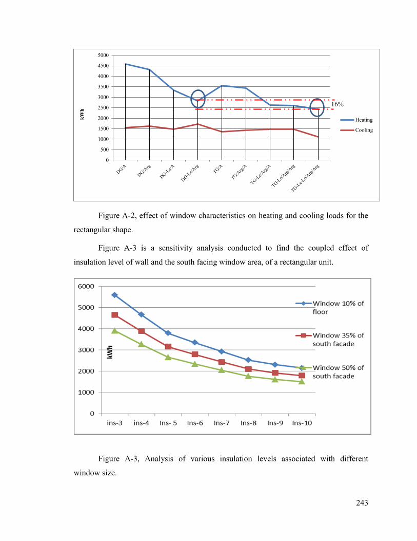
243
Figure A-2, effect of window characteristics on heating and cooling loads for the
rectangular shape.
Figure A-3 is a sensitivity analysis conducted to find the coupled effect of
insulation level of wall and the south facing window area, of a rectangular unit.
Figure A-3, Analysis of various insulation levels associated with different
window size.
0
500
1000
1500
2000
2500
3000
3500
4000
4500
5000
kW
h
Heating
Cooling
16%

244
Appendix B
Roofs of L and L Variant Shapes
L shape and L variants are by their nature more complex than rectangular shape,
and their roofs offer the possibility of design with various tilt angles and orientation (in
the case of L variants)- as shown in previous chapters. The purpose of this section is only
to illustrate possibilities and flexibility of design; however the extra complexity is
probably not justified for small buildings such as housing units.
Split-surface roofs
An attempt is made to apply the concept of multifaceted roofs to L shape. Two
possibilities are considered:
1) To consider a rectangular roof for the L shape. With small depth ratio it is
possible to avoid cutting out the recess. This results in an overhang over the
recessed part of the façade (Fig. B-1 a). For larger depth ratios the recess can be
cut out (Fig. B-1b).
2) The second approach (which can be applied to L variants as well - Fig. B-3) is to
consider the roof of the wing and of the main branch as two separate plate roofs.
Each plate can be then designed at different tilt angle (see Fig. B-2).
First approach: Rectangular shape roof- with or without recess.
L shape roof can be designed in the same method as a rectangular roof. A part can
serve as overhang (Fig. B-1a), or the recess can be cut out (Fig. B-1b).

245
In the case where a rectangular roof is used, the same principle of multifaceted
roof used for the rectangular shape presented in Chapter V can be applied. In this case, it
is recommended that the plate dimensions fit the dimensions of the façades of L shape,
for better architectural design.
For the roof where the recess is cut out, three tilt angles are used: 35°, 40° and
45°. Each row of PV panels is characterized by a different tilt angle (see Fig. B-1). A
disadvantage of this design is that it can result in a higher roof (compared to the
rectangular shape) implying a large attic, and larger amount of materials as compared to
the semi-hip roof design of L shape, employed throughout the research.
Figure B-1 , (a) rectangular roof, (b) roof with the recess cut out
Second Approach: Split Gable roofs
This part shows only few possibilities and not all the combinations that can be
obtained. The focus is the type of roofs that can be designed for L and a few L variants.
15°
S
ide plates
BIPV/T
15°
(a) (b)
Row of PVpanels

246
In this approach, the wing and the main branch roofs are designed as separate gable roofs
which may have the same or different tilt angles. This is shown in Figure B-2 a and b for
L shape, and B-2 c for L variant (V-SW30).
The main problem in this design option is that with large tilt angle the wing roof
may be considerably higher than the main branch roof, shading therefore its BIPV/T
system (see figure B-2 b and c). This can be modified by reducing the surface area of the
wing roof. But in this case an assessment should be done to find whether this option still
beneficial (complexity / aesthetic/ energy generation).
Figure B-2 , (a) rectangular roof, (b) roof with the recess cut out ; (c) L variant with a large
wing surface
Folded Plate roofs
This is not easy to apply. An iterative design process needs to be applied that
coordinates roof design with plan design to optimize both electricity generation and
(
c)
(
b)
(
a)

247
functional space. Some attempts are made here at designs of selected L variants ( V-
SW30 and V-SW60), and L shape. The roof designs are limited only for plates with 30°
orientations.
Figure B-3, folded plates L and L variants roof
Various additional possibilities of roofs of L and L variants are possible. Some of
these are presented in Figure B-4.
Figure B-4 – Additional possibilites of roof designs

248
Appendix C
Sensitivity Analysis of the Weight Assignment-Evaluation System
A sensitivity analysis is performed to identify the effect of weight assignment for
the evaluation system of the design alternatives (proposed in chapter VI). Seven different
alternatives, where weight of performance criteria is changed arbitrarily, and the
evaluation of shape corresponding to these alternatives are presented below.
The results indicate that alternatives where heating consumption weight is lower
than that of the cooling consumption (Alternatives 1, 2 and 3) or where there is no
significant difference between the weights of these two criteria, the sum of the points
gathered by the shapes is not significantly affected (≤5%, as compared to the base case-
the example presented in Chap VI- see Fig. C2). Alternatives (such as Alt.7- see Fig. C1)
where cooling consumption is dominant (double the value of heating consumption), and
where the weight of electricity generation criteria is reduced, favor shapes with small
aspect ratio and large depth ratio (which cast shade on the south façade), which is
expected. Some of the results of the sensitivity analysis are presented below, in tables of
evaluation of shapes, and in Figures C1 and C2.
Table C1, Weight assignments for different alternatives
Alternatives
Weights
Heating
Consumption
Cooling
Consumption
Electricity
generation
Shift of Peak
Generation
Alt0 2 1 3 3
Alt1 2.2 1.3 2.9 0
Alt2 2.2 1.3 2.9 1.5
Alt3 1.9 1.5 2.5 2.5
Alt4 1.5 2 2.5 2.5
Alt5 1 2 2.3 2.3
Alt6 1 2 3 2.3
Alt7 1 3 2 1
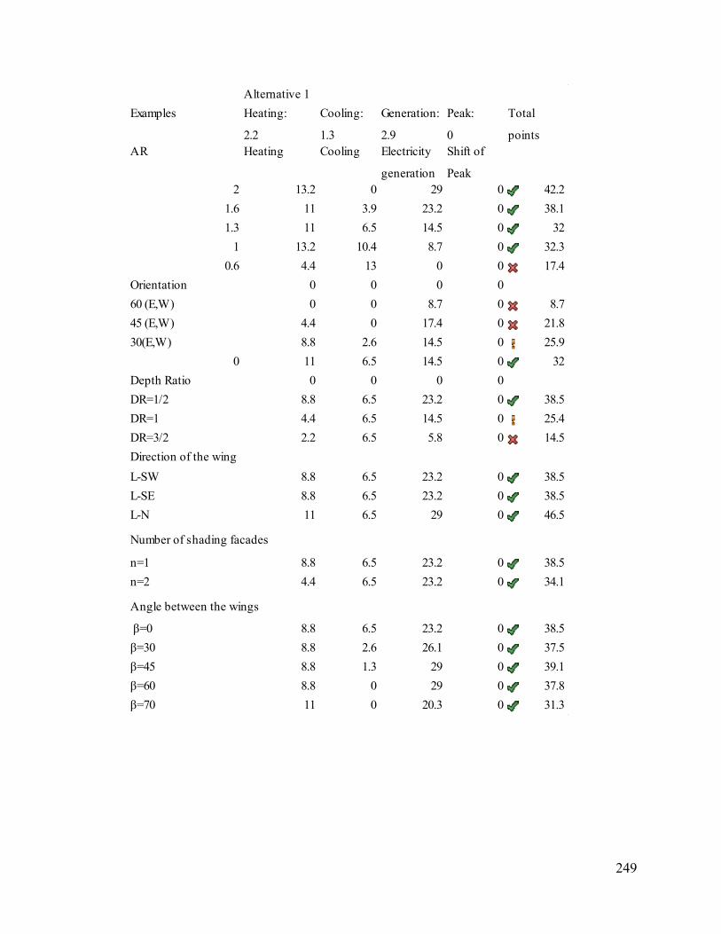
249
Alternative 1
Examples Heating:
2.2
Cooling:
1.3
Generation:
2.9
Peak:
0
Total
points
AR Heating Cooling Electricity
generation
Shift of
Peak
2 13.2 0 29 0 42.2
1.6 11 3.9 23.2 0 38.1
1.3 11 6.5 14.5 0 32
1 13.2 10.4 8.7 0 32.3
0.6 4.4 13 0 0 17.4
Orientation 0 0 0 0
60 (E,W) 0 0 8.7 0 8.7
45 (E,W) 4.4 0 17.4 0 21.8
30(E,W) 8.8 2.6 14.5 0 25.9
0 11 6.5 14.5 0 32
Depth Ratio 0 0 0 0
DR=1/2 8.8 6.5 23.2 0 38.5
DR=1 4.4 6.5 14.5 0 25.4
DR=3/2 2.2 6.5 5.8 0 14.5
Direction of the wing
L-SW 8.8 6.5 23.2 0 38.5
L-SE 8.8 6.5 23.2 0 38.5
L-N 11 6.5 29 0 46.5
Number of shading facades
n=1 8.8 6.5 23.2 0 38.5
n=2 4.4 6.5 23.2 0 34.1
Angle between the wings
β=0 8.8 6.5 23.2 0 38.5
β=30 8.8 2.6 26.1 0 37.5
β=45 8.8 1.3 29 0 39.1
β=60 8.8 0 29 0 37.8
β=70 11 0 20.3 0 31.3

250
Alternative 2
Examples Heating:
2.2
Cooling:
1.3
Generation:
2.9
Peak:
1.5
Total
points
AR Heating Cooling Electricity
generation
Shift of
Peak
2 13.2 0 29 0 42.2
1.6 11 3.9 23.2 0 38.1
1.3 11 6.5 14.5 0 32
1 13.2 10.4 8.7 0 32.3
0.6 4.4 13 0 0 17.4
Orientation 0
60 (E,W) 0 0 8.7 4.5 13.2
45 (E,W) 4.4 0 17.4 3 24.8
30(E,W) 8.8 2.6 14.5 2.25 28.15
0 11 6.5 14.5 0 32
Depth Ratio 0
DR=1/2 8.8 6.5 23.2 0 38.5
DR=1 4.4 6.5 14.5 0 25.4
DR=3/2 2.2 6.5 5.8 0 14.5
Direction of the wing 0
L-SW 8.8 6.5 23.2 0 38.5
L-SE 8.8 6.5 23.2 0 38.5
L-N 11 6.5 29 0 46.5
Number of shading facades0
n=1 8.8 6.5 23.2 0 38.5
n=2 4.4 6.5 23.2 0 34.1
Angle between the wings 0
β=0 8.8 6.5 23.2 0 38.5
β=30 8.8 2.6 26.1 2.25 39.75
β=45 8.8 1.3 29 3 42.1
β=60 8.8 0 29 4.5 42.3
β=70 11 0 20.3 4.5 35.8

251
Alternative 3
Examples Heating :
1.9
Cooling:
1.5
Generation:
2.5
Peak:
2.5
AR Heating Cooling Electricity
generation
Shift of
Peak
Total points
2 11.4 0 25 0 36.4
1.6 9.5 4.5 20 0 34
1.3 9.5 7.5 12.5 0 29.5
1 11.4 12 7.5 0 30.9
0.6 3.8 15 0 0 18.8
Orientation
60 (E,W) 0 0 7.5 7.5 15
45 (E,W) 3.8 0 15 5 23.8
30(E,W) 7.6 3 12.5 3.75 26.85
0 9.5 7.5 12.5 0 29.5
Depth Ratio
DR=1/2 7.6 7.5 20 0 35.1
DR=1 3.8 7.5 12.5 0 23.8
DR=3/2 1.9 7.5 5 0 14.4
Direction of the wing
L-SW 7.6 7.5 20 0 35.1
L-SE 7.6 7.5 20 0 35.1
L-N 9.5 7.5 25 0 42
Number of shading facades
n=1 7.6 7.5 20 0 35.1
n=2 3.8 7.5 20 0 31.3
Angle between the wings o
β=0 7.6 7.5 20 0 35.1
β=30 7.6 3 22.5 3.75 36.85
β=45 7.6 1.5 25 5 39.1
β=60 7.6 0 25 7.5 40.1
β=70 9.5 0 17.5 7.5 34.5

252
Alternative 4
Examples Heating :
1.5
Cooling:
2
Generation:
2.5
Peak:
2.5
AR Heating Cooling Electricity
generation
Shift of Peak Total points
2 9 0 25 0 34
1.6 7.5 6 20 0 33.5
1.3 7.5 10 12.5 0 30
1 9 16 7.5 0 32.5
0.6 3 20 0 0 23
Orientation 0
60 (E,W) 0 0 7.5 7.5 15
45 (E,W) 3 0 15 5 23
30(E,W) 6 4 12.5 3.75 26.25
0 7.5 10 12.5 0 30
Depth Ratio 0
DR=1/2 6 10 20 0 36
DR=1 3 10 12.5 0 25.5
DR=3/2 1.5 10 5 0 16.5
Direction of the wing
L-SW 6 10 20 0 36
L-SE 6 10 20 0 36
L-N 7.5 10 25 0 42.5
Number of shading facades
n=1 6 10 20 0 36
n=2 3 10 20 0 33
Angle between the wings
β=0 6 10 20 0 36
β=30 6 4 22.5 3.75 36.25
β=45 6 2 25 5 38
β=60 6 0 25 7.5 38.5
β=70 7.5 0 17.5 7.5 32.5

253
Alternative 5
Examples Heating :
1
Cooling:
2
Generation
2.3
Peak:
2.3
AR Heating Cooling Electricity
generation
Shift of
Peak
Total
points
2 6 0 23 0 29
1.6 5 6 18.4 0 29.4
1.3 5 10 11.5 0 26.5
1 6 16 6.9 0 28.9
0.6 2 20 0 0 22
Orientation
60 (E,W) 0 0 6.9 6.9 13.8
45 (E,W) 2 0 13.8 4.6 20.4
30(E,W) 4 4 11.5 3.45 22.95
0 5 10 11.5 0 26.5
Depth Ratio
DR=1/2 4 10 18.4 0 32.4
DR=1 2 10 11.5 0 23.5
DR=3/2 1 10 4.6 0 15.6
Direction of the wing
L-SW 4 10 18.4 0 32.4
L-SE 4 10 18.4 0 32.4
L-N 5 10 23 0 38
Number of shading facades
n=1 4 10 18.4 0 32.4
n=2 2 10 18.4 0 30.4
Angle between the wings
β=0 4 10 18.4 0 32.4
β=30 4 4 20.7 3.45 32.15
β=45 4 2 23 4.6 33.6
β=60 4 0 23 6.9 33.9
β=70 5 0 16.1 6.9 28

254
Alternative 6
Examples Heating :
1
Cooling:
2
Generation:
3
Peak:
2.3
AR Heating Cooling Electricity
generation
Shift of
Peak
Total
points
2 6 0 30 0 36
1.6 5 6 24 0 35
1.3 5 10 15 0 30
1 6 16 9 0 31
0.6 2 20 0 0 22
Orientation 0
60 (E,W) 0 0 9 6.9 15.9
45 (E,W) 2 0 18 4.6 24.6
30(E,W) 4 4 15 3.45 26.45
0 5 10 15 0 30
Depth Ratio 0
DR=1/2 4 10 24 0 38
DR=1 2 10 15 0 27
DR=3/2 1 10 6 0 17
Direction of the wing 0
L-SW 4 10 24 0 38
L-SE 4 10 24 0 38
L-N 5 10 30 0 45
Number of shading facades0
n=1 4 10 24 0 38
n=2 2 10 24 0 36
Angle between the wings 0
β=0 4 10 24 0 38
β=30 4 4 27 3.45 38.45
β=45 4 2 30 4.6 40.6
β=60 4 0 30 6.9 40.9
β=70 5 0 21 6.9 32.9

255
Alternative 7
Examples Heating :
1
Cooling:
3
Generation
2
Peak:
1
AR Heating Cooling Electricity
generation
Shift of Peak Total points
2 6 0 20 0 26
1.6 5 9 16 0 30
1.3 5 15 10 0 30
1 6 24 6 0 36
0.6 2 30 0 0 32
Orientation
60 (E,W) 0 0 6 3 9
45 (E,W) 2 0 12 2 16
30(E,W) 4 6 10 1.5 21.5
0 5 15 10 0 30
Depth Ratio 0 0 0
DR=1/2 4 15 16 0 35
DR=1 2 15 10 0 27
DR=3/2 1 15 4 0 20
Direction of the wing 0 0 0 0
L-SW 4 15 16 0 35
L-SE 4 15 16 0 35
L-N 5 15 20 0 40
Number of shading facades0 0 0
n=1 4 15 16 0 35
n=2 2 15 16 0 33
Angle between the wings
β=0 4 15 16 0 35
β=30 4 6 18 1.5 29.5
β=45 4 3 20 2 29
β=60 4 0 20 3 27
β=70 5 0 14 3 22

256
Figure C1, representation of all points accumulated by each shapes, for each alternative of
weight assignment
0
5
10
15
20
25
30
35
40
45
50
2
1.6
1.3 1
0.6
60
(E,
W)
45
(E,
W)
30
(E,W
)
0(E
,W)
DR
=1/2
DR
=1
DR
=3/2
L-SW L-SE L-N
n=1
n=2
β=0
β=3
0
β=4
5
β=6
0
β=7
0
AR Orientation DR WingDirection
n β
Rectangle Non- Convex shapes
Tota
l po
ints
Alt0
Alt.1
Alt2
Alt3
Alt4
Alt5
Alt6
Alt7
Alt.7 (cooling weight is dominant)
is the the best option for shapes
with small aspect ration, and for
non convex shapes with large depth
ratio

257
Figure C2, comparison of all alternatives of weight assignments to the base case (the example
presented in Chapter VI)

258
Glossary
Aspect Ratio: Ratio of equatorial facing façade to the perpendicular façade.
Building-Integrated: A component that is designed to be part of a façade or roof. In this
work, it refers to solar collectors (photovoltaic or thermal or both).
Coefficient of performance (COP)-Heat pump: The ratio of the rate of energy output
of the heat pump to the rate of energy input, under specific operating conditions
(ASHRAE Standard, 90.1, 2007).
Design Day (DD): A day having representative climatic conditions for specific
objectives design. In this document two design days are selected to represent sunny
winter and summer days (Hong et al, 1999).
Depth Ratio: In non-convex housing unit shapes having two or more wings, where wings
are mutually shading, the depth ratio is the ratio of the width of the shade-casting façade
(non-equatorial facing) to the width of the shaded façade (equatorial facing).
Energy performance: Energy performance criteria of buildings and neighborhood
includes total annual energy consumption, energy generation (electricity and heat) and
time spread of peak electricity generation
Exposed facade: In a non-convex shapes exposed façade refers to the equatorial or near-
equatorial façade of a shading wing that is perpendicular to the shade casting façade.
L Variations: L shapes with different angles between the wings.

259
Non-convex Shape: A shape where at least one line segment connecting two points
along the boundary lies outside the shape.
Net-zero energy homes (NZEH): Houses which, on an annual basis, produce as much
energy from renewable sources as they consume.
Obtuse Angle: Special L variant with large value of the angle β between the wings
(β=70º is adopted in the study).
Orientation Angle: The orientation angle of a surface is defined as the angle between
equatorail and the projection on a horizontal plane of the normal to this surface.
Passive solar strategy: The act of collecting solar energy and storing it within a
building’s structure to offset energy demand without dependence on active systems.
Planar Obstruction Angle (POA): POA concept represents the angle between the center
of the equatorial façade of the shaded unit and the closest corner of the shading unit.
Shaded facades: Facade in non-convex geometries that are shaded by other facades. In
this research they refer to the equatorial facing facades, shaded by the adjacent one.
Solar Potential: Passive potential involves irradiation and transmission of heat and
daylighting by fenestration of near-equatorial-facing facades. Active potential consists of
generation of both electricity and thermal energy employing building integrated
photovoltaic thermal systems (BIPV/T).
Space load (heating and cooling): The amount of energy that must be added to or
extracted from a space to maintain thermal comfort (ASHRAE, 2005).
Summer Design Day (SDD): Represents an extreme hot sunny day.

260
Tilt Angle: Tilt angle of a surface is the angle between the normal to the surface and the
vertical direction.
Winter Design Day (WDD): Represents an extreme cold sunny day.