INVESTIGATION OF A PULSED PLASMA THRUSTER PLUME USING

A QUADRUPLE LANGMUIR PROBE TECHNIQUE

by

Jurg C. Zwahlen

A Thesis

Submitted to the Faculty

of the

WORCESTER POLYTECHNIC INSTITUTE

in partial fulfillment of the requirements for the

Degree of Master of Science

in

Mechanical Engineering

November 2002

APPROVED: ______________________________________________ Dr. Nikolaos A. Gatsonis, Advisor Associate Professor, Mechanical Engineering Department ______________________________________________ John Blandino, Committee Member Assistant Professor, Mechanical Engineering Department ______________________________________________ David Olinger, Committee Member Associate Professor, Mechanical Engineering Department ______________________________________________ Eric Pencil, Committee Member NASA Glenn Research Center ______________________________________________ Michael Demetriou, Graduate Committee Representative Assistant Professor, Mechanical Engineering Department

Abstract The rectangular pulsed plasma thruster (PPT) is an electromagnetic thruster that ablates

Teflon propellant to produce thrust in a discharge that lasts 5-20 microseconds. In order to

integrate PPTs onto spacecraft, it is necessary to investigate possible thruster plume-spacecraft

interactions. The PPT plume consists of neutral and charged particles from the ablation of the

Teflon fuel bar as well as electrode materials. In this thesis a novel application of quadruple

Langmuir probes is implemented in the PPT plume to obtain electron temperature, electron

density, and ion speed ratio measurements (ion speed divided by most probable thermal speed).

The pulsed plasma thruster used is a NASA Glenn laboratory model based on the LES

8/9 series of PPTs, and is similar in design to the Earth Observing-1 satellite PPT. At the 20 J

discharge energy level, the thruster ablates 26.6 µg of Teflon, creating an impulse bit of 256 µN-

s with a specific impulse of 986 s.

The quadruple probes were operated in the so-called current mode, eliminating the need

to make voltage measurements. The current collection to the parallel to the flow electrodes is

based on Laframboise’s theory for probe to Debye length ratios of 5 100p Dr λ≤ ≤ and on the

thin-sheath theory for r . The ion current to the perpendicular probe is based on a

model by Kanal and is a function of the ion speed ratio, the applied non-dimensional potential

and the collection area. A formal error analysis is performed using the complete set of nonlinear

current collection equations. The quadruple Langmuir probes were mounted on a computer

controlled motion system that allowed movement in the radial direction, and the thruster was

mounted on a motion system that allowed angular variation. Measurements were taken at 10, 15

and 20 cm form the Teflon fuel bar face, at angles up to 40 degrees off of the centerline axis at

discharge energy levels of 5, 20, and 40 J. All data points are based on an average of four PPT

/ 100p Dλ >

I

pulses.

Data analysis shows the temporal and spatial variation in the plume. Electron

temperatures show two peaks during the length of the pulse, a trend most evident during the 20 J

and 40 J discharge energies at 10 cm from the surface of the Teflon fuel bar. The electron

temperatures after the initial high temperature peak are below 2 eV. Electron densities are

highest near the thruster exit plane. At 10 cm from the Teflon surface, maximum electron

densities are 1.04x1020 ± 2.8x1019 m-3, 9.8x1020 ± 2.3x1020 m-3, and 1.38x1021 ± 4.05x1020 m-3

for the 5 J, 20 J and 40 J discharge energy, respectively. The electrons densities decrease to

2.8x1019 ± 8.9x1018 m-3, 1.2x1020 ± 4.2x1019 m-3, and 4.5x1020 ± 1.2x1020 m-3 at 20 cm for the 5

J, 20 J, and 40 J cases, respectively. Electron temperature and density decrease with increasing

angle away from the centerline, and with increasing downstream distance. The plume is more

symmetric in the parallel plane than in the perpendicular plane.

Ion speed ratios are lowest near the thruster exit, increase with increasing downstream

distance, but do not show any consistent angular variation. Peak speed ratios at a radial distance

of 10 cm are 5.9±3.6, 5.3±0.39, and 4.8±0.41 for the 5 J, 20 J and 40 J discharge energy,

respectively. The ratios increase to 6.05±5.9, 7.5±1.6, and 6.09±0.72 at a radial distance of 20

cm. Estimates of ion velocities show peak values between 36 km/s to 40 km/s, 26 km/s to 30

km/s, and 26 km/s to 36 km/s.

II

Acknowledgments This thesis is a continuation of the work I did as an undergraduate here at WPI, and for

that work I thank my project partners Jeff Hamel and Matt Krumanaker. For all the times I went

out to Cleveland, and for the guidance and assistance through the entirety of this thesis, I give

much thanks to Eric Pencil at NASA Glenn. I also must thank Hani Kamhawi who provided

much advice and help through the experimentation process.

Many thanks go to Adrian Wheelock and Larry Byrne for all the assistance with code

debugging, experimental assistance, and general support, I could not have done this work

without you.

Professor Nikos Gatsonis has shown me much through the years of my graduate degree.

To him I give my gratitude for the commitment, advice, assistance and support. I have learned

much, all to my benefit, and am greatly appreciative. To all the guys in the lab including Anton

Spirkin, Tom Roy, Andrew Syriyali, Ray Janowski, and Bill Freed, thanks for the friendship and

constant levity. May you all succeed in your endeavors. Much thanks goes to Barbara Edilberti,

Janice dresser, Pam St Louis, and Barbara Furman who made the world around me run smoothly

from within the chilled regions of Higgins. Thanks also to my committee members, John

Blandino, Eric Pencil and Dave Olinger for the assistance with the final stages of this thesis.

To the non-engineers I should give the most thanks for all the support. My mother, father,

and brother all deserve my thanks for their constant support and blessings. I have said hello to

many friends since coming here, and to all of you I owe an enormous debt of gratitude. Thank

you for the laughter, the couches, the food, and your time. To you I say good luck and God bless,

may you find your future to your enjoyment. My final and greatest thanks goes to Lourinda, for

always being there to pull me up and through. Thank you.

III

Table Of Contents

Abstract______________________________________________________________________I

Acknowledgments____________________________________________________________ III

Table Of Contents ___________________________________________________________ IV

List Of Tables and Figures ____________________________________________________ VI

Nomenclature________________________________________________________________ 1

1 Introduction _____________________________________________________________ 4

1.1 Review of Ablative PPT Plume Experiments ____________________________________ 7

1.2 Objectives and Approach ____________________________________________________ 9

2 Experimental Setup, Diagnostics, and Procedures______________________________ 12

2.1 Experimental Setup and Facilities ____________________________________________ 12

2.1.1 NASA GRC Pulsed Plasma Thruster _________________________________________________12

2.1.2 Vacuum Facility _________________________________________________________________13

2.1.3 Automated Positioning System______________________________________________________14

2.2 Quadruple Langmuir Probes ________________________________________________ 15

2.2.1 Quadruple Langmuir Probe Theory __________________________________________________16

2.2.2 Quadruple Langmuir Probe Design __________________________________________________20

2.2.3 Cabling and Diagnostics ___________________________________________________________22

2.3 Experimental Procedures ___________________________________________________ 23

2.3.1 Probe Cleaning __________________________________________________________________23

2.3.2 Data Sampling __________________________________________________________________24

IV

3 Data Reduction, Analysis and Results _______________________________________ 27

3.1 Current Sensitivity ________________________________________________________ 27

3.2 Data Reduction Algorithm __________________________________________________ 28

3.3 Uncertainty and Error Analysis______________________________________________ 30

3.4 Regression Analysis ________________________________________________________ 44

3.5 Quadruple Langmuir Probe Data Analysis ____________________________________ 45

3.5.1 Electron Density and Temperature of a PPT Plume ______________________________________46

3.5.2 Ion Speed Ratio and Ion Velocity of a PPT Plume_______________________________________62

4 Summary and Recommendations ___________________________________________ 65

4.1 Summary of Experimental Setup, Diagnostics and Procedures ____________________ 65

4.2 Summary of Data Reduction, Analysis and Results ______________________________ 65

4.2.1 Results and Discussion ____________________________________________________________66

4.3 Recommendations _________________________________________________________ 67

References _________________________________________________________________ 69

V

List Of Tables and Figures

Table 1 - Operational characteristics of the NASA GRC lab model Pulsed Plasma Thruster ....... 9

Table 2 Non-dimensional parameters of a quadruple probe with r 41.25 10p−= × m, s 310−= m

in a PPT plume...................................................................................................................... 33

Table 3 - Mean, standard error and random uncertainty for φ12 , φ13 , and 14φ ............................ 36

Figure 1.1 Schematic of a rectangular Teflon ablative PPT and its plume..................................... 5

Figure 2.1 NASA GRC lab model PPT (Nozzle not Shown) ....................................................... 13

Figure 2.2 CW-19 Vacuum Facility.............................................................................................. 14

Figure 2.3 Schematic of Automated Positioning System ............................................................. 15

Figure 2.4 Voltage Mode QLP Circuit ......................................................................................... 17

Figure 2.5 Current Mode QLP Circuit.......................................................................................... 17

Figure 2.6 Schematic of a Quadruple Langmuir Probe ................................................................ 21

Figure 2.7 Electrical Diagram of Experimental Facility............................................................... 23

Figure 2.8 Perpendicular Plane Points .......................................................................................... 25

Figure 2.9 Parallel Plane Points .................................................................................................... 25

Figure 3.1 Typical quadruple Langmuir probe current trace with evaluated plasma parameters.

Measurements taken at r =10 cm and θ =90 deg in the plume of a 20-J laboratory PPT.... 30

Figure 3.2 –Measurements of φ , φ , and φ taken at r =20 cm and =90 deg in the plume of

a 5 Joule laboratory PPT. ...................................................................................................... 37

12 13 14 θ

Figure 3.3 - Measurements of φ , φ , and φ taken at r =20 cm and =90 deg in the plume of

a 20 Joule laboratory PPT. .................................................................................................... 38

12 13 14 θ

VI

Figure 3.4 - Measurements of φ , φ , and φ taken at r =20 cm and =90 deg in the plume of

a 40 Joule laboratory PPT. .................................................................................................... 39

12 13 14 θ

Figure 3.5 - Absolute value of errors , , and as determined by individual

uncertainties as well as the full contribution from all uncertainties. Measurements taken at

=10 cm and =90 deg in the plume of a 40-J laboratory PPT......................................... 42

( )eT t∆ ( )en t∆ ( )iS t∆

r θ⊥

Figure 3.6 –Error for combination of uncertainties. Measurements taken at r =10 cm and θ =90

deg in the plume of a 40-J laboratory PPT ........................................................................... 43

⊥

Figure 3.7 - Plot of n , n t , and n t . Measurements taken at r =10 cm

and θ =90 deg in the plume of a 40-J laboratory PPT......................................................... 44

( )e t ( ),e p pr r±∆ ( ,e I I±∆ )

⊥

Figure 3.8 – Removal of outliers in T from the quadruple Langmuir probe data set at r =10 cm

and θ =90 deg in the plume of a 20-J laboratory PPT.......................................................... 45

e

Figure 3.9 - Typical current trace with evaluated plasma parameters and error bars.

Measurements taken at r =10 cm and θ =90 deg in the parallel plane of a 20-J laboratory

PPT........................................................................................................................................ 46

Figure 3.10 Electron temperature, electron density and ion speed ratio from quadruple probe

measurements taken on the parallel plane of a 5-J laboratory PPT plume. .......................... 54

Figure 3.11 Electron temperature, electron density and ion speed ratio from quadruple probe

measurements taken on the perpendicular plane of a 5-J laboratory PPT plume. ................ 55

Figure 3.12 Electron temperature, electron density and ion speed ratio from quadruple probe

measurements taken on the parallel plane of a 20-J laboratory PPT plume. ........................ 56

Figure 3.13 Electron temperature, electron density and ion speed ratio from quadruple probe

measurements taken on the perpendicular plane of a 20-J laboratory PPT plume. .............. 57

Figure 3.14 Electron temperature, electron density and ion speed ratio from quadruple probe

VII

measurements taken on the parallel plane of a 40-J laboratory PPT plume. ........................ 58

Figure 3.15 Electron temperature, electron density and ion speed ratio from quadruple probe

measurements taken on the perpendicular plane of a 40-J laboratory PPT plume. .............. 59

Figure 3.16 - Spatial variation of T , n , and S in the plume of a laboratory model

PPT........................................................................................................................................ 60

maxe

maxe

maxi

Figure 3.17 Discharge current, T at r =10 cm, r =20 cm and = 90 degrees in the plume

of a laboratory PPT operating at discharge energies of 5 J, 20 J, and 40 J........................... 61

e en iS θ

Figure 3.18 Quadruple and Triple Langmuir probe data in the parallel plane of a 40 J laboratory

PPT plume............................................................................................................................. 62

Figure 3.19 Evaluated ion speeds at centerline in the plume of a laboratory PPT operating at

discharge energies of 5 J, 20 J, and 40 J. .............................................................................. 64

VIII

Nomenclature

( )A ⊥ collection area for the parallel (perpendicular) to the flow electrode.

pA probe area

iC most probably ion thermal velocity

sd probe sheath thickness

E discharge energy level

e electron charge (1.602 ) 1910 C−×

g gravitational acceleration ( 2m9.806 s )

( )DI t discharge current

( )pI t total probe current

( )( )i e pI t ion, (electron) probe current

( ), 0i eJ current density of ions (electrons)

k Boltzmann constant ( 23 J10 K

−×1.3806 )

stKn Knudsen number for s-t collisions

pL probe length

mi mass flow rate

( )i em mass of ion (electron)

( ), ,en r tθ electron number density

( )max ,en r θ maximum electron density during a pulse

1

( )0 ,en r θ initial guess of electron density

Pn quadruple Langmuir probe electrode n=1,2,3,4

r radial distance downstream from the center of Teflon surface to the Langmuir

probe

pr probe radius

s probe spacing

( ), ,iS r tθ ratio of ion speed to most probably ion velocity

( )max ,iS r θ maximum speed ratio during a pulse

( )0 ,iS r θ initial guess of speed ratio

t time

( ), ,eT r tθ electron temperature

(max ,eT r θ) maximum electron temperature

( )0 ,eT r θ initial guess of electron temperature

iT ion temperature

iu ion speed

dnV voltage difference between probes 1 and n=2,3,4

iZ number charge of ion i

( )A±∆ uncertainty in variable A

0ε permitivity of free space

( )p tφ potential of probe p

( )s tφ plasma (or space) potential

( )ps tφ voltage difference between probe p and plasma potential

2

1pφ mean voltage between probe 1 and probe n

stλ mean free path for collisions between species s and t

Dλ Debye length

Lτ end-effect parameter

( )θ ⊥ polar angle in the parallel (perpendicular) plane measured from the center of the

Teflon surface

stν collision frequency between species s and t

pχ non-dimensional potential at a probe p

3

1 Introduction

Satellites use onboard propulsion for a variety of functions, such as attitude control, orbit

transfers and maintenance, instrument pointing and solar panel positioning. On-board propulsion

is achieved by either chemical or electric thrusters. Chemical thrusters generate thrust via nozzle

expansion of a gas produced by the combustion of a solid or fluid propellant. These chemical

thrusters are generally complex devices, with many moving parts and sometimes-volatile fuels

which must be stored properly. While chemical thrusters can produce high thrust, they have low

specific impulses, a measure of the performance of a thruster as given by the ratio of thrust to

propellant weight flow rate sp hrust m= iI T . Electrical thrusters generate thrust by accelerating

an ionized gas via electrostatic or electromagnetic forces. This method is not capable of

generating high thrust at modest power levels, but has a greater specific impulse, usually above

500s, whereas chemical thrusters have a specific impulse below 500 seconds.

g

Pulsed plasma thrusters (PPTs) are a type of electrical thruster that produces thrust by the

acceleration of an ionized gas primarily as a result of electromagnetic forces. PPTs were

designed in the 1950’s in the Soviet Union and shortly thereafter in the United States. The two

types of PPTs currently in production are Teflon ablative with a rectangular or cylindrical

electrode geometry. This study investigates the plumes of rectangular Teflon ablative PPTs, one

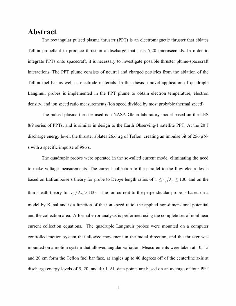
of the mechanically simplest types of electric thruster. As Figure 1.1 shows, the only moving part

is the fuel feed spring. The mechanical simplicity contributes to the reliability of the solid fuel

PPT as well as its long operational life. The ablative PPT produces thrust by accelerating ionized

Teflon gas electro-magnetically. The Teflon fuel bar is spring fed between two electrodes, one of

which has a spark plug imbedded in its base as seen in Figure 2.1. The capacitor is charged to the

desired level, then the spark plug fires producing electrons in the space between the two

4

electrodes thus allowing a discharge between the electrodes. The discharge ablates and ionizes a

small mass off the surface of the Teflon fuel bar, and induces an electromagnetic field between

the electrodes. There is a Lorentz force or B×J , interaction between the electromagnetic field

and the ionized Teflon, which accelerates the plasma and produces the thrust. Any neutrals

created from the ablation are accelerated by gasdynamic expansion. The ablative PPT, similar to

the one used in this thesis, is a very reliable device as was demonstrated when lab model PPTs

were removed from uncontrolled storage after 20 years, and successfully fired at the NASA

Lewis Research Center (now NASA Glenn Research Center) [McGuire, et al., 1995].

Electrodes

SpacecraftSurface

Plume Effluents:

Charged and Neutral: C, F, C FParticulates: sputtered and eroded materialsCharge exchange ions and neutrals

x y

Potential Plume / Spacecraft Interactions

Surface InteractionsBackflow contaminationCommunications signal

Teflon

CEXCollisions

++

+

+

+

NCEX

IP

N

ICEX

I

N

I

Typical Characteristics

Isp: 1000 sPulse Duration: 15 sMass Ablated: 25 gDischarge Energy: 20 J

µµ

Figure 1.1 Schematic of a rectangular Teflon ablative PPT and its plume

PPTs have been used on previous flight programs, and are capable of taking over for

several spacecraft applications. Some suggested PPT applications include: attitude control, where

PPTs would replace mechanical systems like momentum wheels and torque rods, and chemical

propulsion systems; orbit transfers and maintenance, where PPTs would replace the heavier

chemical thruster systems and be used to raise a satellite from the shuttle orbit, or to de-orbit a

spacecraft. PPTs can also be used for position maintenance of a formationb of satellites or in

missions requiring very fine positioning [Myers, et al., 1994].

5

The first recorded use of a pulsed plasma thruster was in 1964, when six PPTs were

flown on the Soviet Zond-2 satellite to provide positioning for its solar arrays. The satellite was

launched on November 30, 1964, to be used in a Martian flyby mission [Pollard, et al.,1993]. In

the US, Fairchild Hiller Co. and MIT’s Lincoln Lab developed a PPT for the Lincoln

experimental Satellite (LES) 6 satellite, launched on September 26, 1968 [Guman and

Nathanson, 1970]. MIT went on to develop a flight qualified PPT for the LES 8/9 satellites, but

the thrusters were dropped from the program at the last minute. The LES 8/9 thrusters have

become a widely tested device due to their flight qualified design [Myers, et al., 1995].

In 1975, the US Navy used two PPTs on five different TIP/NOVA satellites for drag

compensation. The mission showed that PPTs had minimum effects on solar arrays and no EMI

effects on the spacecraft if designed properly [Myers, et al., 1994]. Fairchild continued PPT

research into the late 1970’s on a millipound thrust level PPT [Guman and Begun, 1978]. PPTs

were also flown for experimental purposes on the Japanese ETS-IV satellite in 1981, to study

EMI effects [Pollard, 1993].

The latest flight with PPTs has been the Earth Observing 1 (EO-1) project in 2001. The

Teflon ablative PPT flown on EO-1 was a rectangular geometry type similar to the LES 8/9

flight qualified PPT. The EO-1 PPT was flown as a technology demonstration, in which the PPT

would replace the function of the pitch axis momentum wheel for three days. The specific

impulse ranges from 650 seconds at 12 W input power to 1400 seconds at 70 W input power

[Arrington, et al. 1999].

None of these PPT missions showed adverse effects of the PPT plume on the spacecraft.

Evaluating the plume over a range of energy levels is also beneficial as plume/spacecraft

interactions may vary with energy level, especially on small spacecraft. The plasma plume

created by the thruster is made up of ionized and neutral particles as shown in Figure 1.1.

6

Possible plume-spacecraft interactions include spacecraft charging from the ions, the deposition

of neutral particles on spacecraft surfaces like solar arrays and optical lenses, spacecraft surface

erosion from high energy ions, possible electromagnetic interference with spacecraft electronics

and communications signals from the ionized plasma, and thermal loading of the spacecraft from

thruster firings. In addition, an investigation of the PPT plume helps characterize thruster

performance for future applications.

This work was is part of a NASA program to investigate PPT plume-spacecraft

interactions. WPI’s PPT program incorporates experimental and computational research to

achieve this goal. The experimental work is conducted in a large vacuum facility at NASA Glenn

Research Center in the Electric Propulsion Laboratory and aids the computational modeling

work. A comprehensive review of this work is given by Gatsonis, et al. [2001]. This thesis

presents an experimental investigation of a solid Teflon PPT plume. This work details the

development of a quadruple Langmuir probe method and its use in measuring electron

temperature, electron density, and ion speed ratio in the PPT plume. The PPT was operated at 5

J, 20 J and 40 J to be consistent with possible PPT applications. Measurements were taken at

radial distances from 10 to 20 cm along angular locations from centerline to 40 degrees off

centerline in planes parallel and perpendicular to the thruster electrodes. This data is compared to

triple Langmuir probe measurements obtained from previous investigations [Eckman, et al.,

2001; Gatsonis, et al., 2002]. To fully understand the scope of this thesis, it is important to

outline previous investigations of ion speed, electron temperature, and electron density of

ablative PPT plumes.

1.1 Review of Ablative PPT Plume Experiments

PPT plume studies started with the LES-6 thruster. The thruster ablated 10 µg at an

operational energy of 1.85 J during a 3 µs pulse, producing a specific impulse of 312 s. Vondra,

7

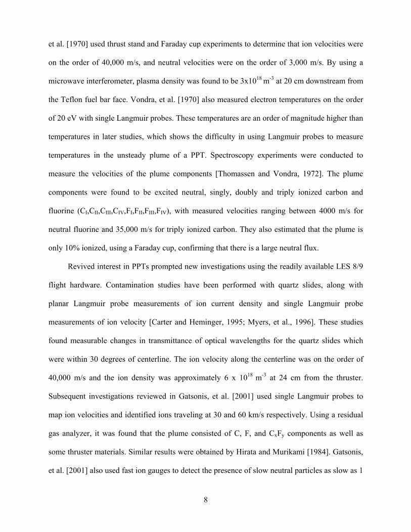
et al. [1970] used thrust stand and Faraday cup experiments to determine that ion velocities were

on the order of 40,000 m/s, and neutral velocities were on the order of 3,000 m/s. By using a

microwave interferometer, plasma density was found to be 3x1018 m-3 at 20 cm downstream from

the Teflon fuel bar face. Vondra, et al. [1970] also measured electron temperatures on the order

of 20 eV with single Langmuir probes. These temperatures are an order of magnitude higher than

temperatures in later studies, which shows the difficulty in using Langmuir probes to measure

temperatures in the unsteady plume of a PPT. Spectroscopy experiments were conducted to

measure the velocities of the plume components [Thomassen and Vondra, 1972]. The plume

components were found to be excited neutral, singly, doubly and triply ionized carbon and

fluorine (CI,CII,CIII,CIV,FI,FII,FIII,FIV), with measured velocities ranging between 4000 m/s for

neutral fluorine and 35,000 m/s for triply ionized carbon. They also estimated that the plume is

only 10% ionized, using a Faraday cup, confirming that there is a large neutral flux.

Revived interest in PPTs prompted new investigations using the readily available LES 8/9

flight hardware. Contamination studies have been performed with quartz slides, along with

planar Langmuir probe measurements of ion current density and single Langmuir probe

measurements of ion velocity [Carter and Heminger, 1995; Myers, et al., 1996]. These studies

found measurable changes in transmittance of optical wavelengths for the quartz slides which

were within 30 degrees of centerline. The ion velocity along the centerline was on the order of

40,000 m/s and the ion density was approximately 6 x 1018 m-3 at 24 cm from the thruster.

Subsequent investigations reviewed in Gatsonis, et al. [2001] used single Langmuir probes to

map ion velocities and identified ions traveling at 30 and 60 km/s respectively. Using a residual

gas analyzer, it was found that the plume consisted of C, F, and CxFy components as well as

some thruster materials. Similar results were obtained by Hirata and Murikami [1984]. Gatsonis,

et al. [2001] also used fast ion gauges to detect the presence of slow neutral particles as slow as 1

8

ms after the discharge pulse had ended, showing an inefficient use of the Teflon propellant.

Eckman, et al. [2001] continued plume studies of a NASA Glenn Research Center lab

model PPT whose operational characteristics are presentedd in Table 1. The lab model PPT is

very similar in size and performance to the EO-1 PPT and was derived from the LES 8/9 PPT.

Triple Langmuir probes were used to take measurements of electron temperature and density at

5, 20 and 40 Joule discharge energies. At 20 cm along the centerline from the Teflon fuel bar

face, the electron densities ranged from 1.0 x 1019 to 4.2 x 1020 for the three energies, and

electron temperatures ranged from 2 to 3.5 eV [Eckman, et al., 2001]. The experiments of

Eckman, et al. [2001] used the triple Langmuir probe voltage method outlined by Chen and

Sekiguchi [1965]. In this traditional approach one of the probes is biased relative to a reference

probe, and one is allowed to float electrically. The resulting voltage between the floating probe

and reference probe and the current in the biased probe are measured, allowing for the evaluation

of T and n . It was found that the floating voltage measurement was susceptible to noise

at the beginning of a PPT discharge. Subsequent work by Byrne, et al. [2001] and Byrne, et al.

[2002] developed the so-called “current mode” triple Langmuir probe also outlined by Chen and

Sekiguchi, 1965 and Chen, 1971. In the “current mode” triple Langmuir probe two probes are

biased in reference to the third, and all three of the probe currents are measured. Details of the

application of the “current mode” triple Langmuir probe, the current collection theory used and

the obtained measurements are presented by Byrne, et al., [2002].

( )e t ( )e t

Discharge Energy (J)

Impulse Bit (µN-s)

Mass Loss/Pulse (µg/pulse)

Specific Impulse (s)

5.3 36 - - 20.5 256 26.6 982 44.0 684 51.3 1360

Table 1 - Operational characteristics of the NASA GRC lab model Pulsed Plasma Thruster

1.2 Objectives and Approach

In order to further the understanding of the ablative PPT plume as well as the thrust

9

production mechanism, the characterization of ion speed is needed. Quadruple Langmuir probes

were chosen as a diagnostic, since they allow the simultaneous measurement of electron

temperature T , electron densityn , and ion speed ratio S defined as e e i

ii

i

uSc

= (1.1)

where is the ion velocity, and c is the ion thermal speed. A quadruple Langmuir probe is a

combination of a triple Langmuir probe and crossed probe. The use of crossed electrostatic

probes in a flowing plasma was first described by Johnson and Murphree [1969]. They utilized

the theory of current collection by a cylindrical probe defined by Kanal [1964]. The first

application of a quadruple Langmuir probe was by Burton, et al. [1993], and provided

measurements of T , , and u in the plume of a pulsed magnetoplasmadynamic

(MPD)thruster. Subsequent implementations of quadruple Langmuir probes on arcjet plumes by

Burton and Bufton [1996] included corrections to the ion current equations to account for multi-

species ions. The latest implementation of quadruple Langmuir probes was in the plume of a

gasdynamic PPT [Burton and Bushman, 1999]. All of the previous implementations of quadruple

Langmuir probes operated in a voltage-mode, where one of the probe electrodes operates at the

floating potential of the plasma. Also, these previous implementations used a current collection

theory that assumed negligible sheath thickness

iu i

e en i

( , and that the probe is operating in

the ion-saturation regime where the ion saturation current is independent of the applied probe

potential.

)1s pd r →

The goal of this thesis is to develop and implement a quadruple Langmuir probe method to

measure ion speed ratio, electron temperature and electron density in the plume of a GRC

laboratory model PPT operating between 5 and 40 Joules. This work considerably extends

previous studies of the laboratory PPT plasma plume as reviewed in Gatsonis, et al. (2001) and

10

compliments the ongoing triple Langmuir probe investigations (Byrne, et al., 2002). The

objectives of this thesis are as follows:

• Design a QLP that can measure ion speed ratio and electron temperature and density of a

NASA GRC lab model PPT using facilities at NASA Glenn Research Center. Implement

the QLPs in the “current mode” using the current collection theory outlined in Gatsonis,

et al. [2002].

• Modify the Byrne, et al. [2001] TLP experimental setup to accommodate QLPs. This

objective includes the modification of the vacuum facility and diagnostics to allow for the

addition of a current measurement, as well as shielding efforts of the experimental setup.

• Develop procedures for data collection and experiment handling. Procedures are

implemented for probe cleaning between firings to deter measurement degradation, for

consistent data acquisition methods, and for data transfer procedures are included.

• Use a QLP to measure i iυ= iS , , and n at angles up to 40 degrees off of

centerline, at 10, 15 and 20 cm from the Teflon fuel bar surface on planes perpendicular

and parallel to the thruster electrodes. Measurements are taken at thruster discharge

energies of 5, 20 and 40 J.

c eT e

• Develop data processing software that will numerically solve the system of equations that

describe the QLP operation and that will simultaneously provide a numerical solution for

the error analysis equations as described in Gatsonis, et al. [2002].

In Chapter Two of this thesis the development of the quadruple Langmuir probe theory, as

well as the experimental setup and procedures are explained. Chapter Three describes the

data processing software and presents the results along with the error and data analysis.

Chapter Four offers a summary of the work, with conclusions and future recommendations.

11

2 Experimental Setup, Diagnostics, and Procedures

2.1 Experimental Setup and Facilities

All measurements were taken at NASA Glenn Research Center in Cleveland, Ohio. A

large vacuum facility in room CW-19 of Building 5 was used to simulate space vacuum. A probe

motion system design used by Byrne, et al. [2001] was modified to handle QLP’s to shorten

experimentation time. The experimental setup, probe circuitry, probe theory and cleaning

procedures related to the quadruple Langmuir probes will be discussed in the following sections.

2.1.1 NASA GRC Pulsed Plasma Thruster

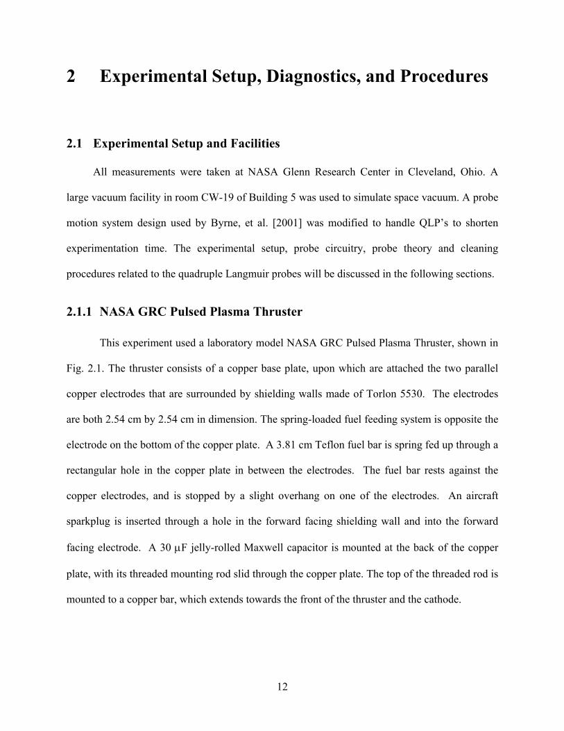
This experiment used a laboratory model NASA GRC Pulsed Plasma Thruster, shown in

Fig. 2.1. The thruster consists of a copper base plate, upon which are attached the two parallel

copper electrodes that are surrounded by shielding walls made of Torlon 5530. The electrodes

are both 2.54 cm by 2.54 cm in dimension. The spring-loaded fuel feeding system is opposite the

electrode on the bottom of the copper plate. A 3.81 cm Teflon fuel bar is spring fed up through a

rectangular hole in the copper plate in between the electrodes. The fuel bar rests against the

copper electrodes, and is stopped by a slight overhang on one of the electrodes. An aircraft

sparkplug is inserted through a hole in the forward facing shielding wall and into the forward

facing electrode. A 30 µF jelly-rolled Maxwell capacitor is mounted at the back of the copper

plate, with its threaded mounting rod slid through the copper plate. The top of the threaded rod is

mounted to a copper bar, which extends towards the front of the thruster and the cathode.

12

The main copper plate, as well as the copper

bar are insulated with Kapton tape and

Kapton shielding, with only the connection

surfaces for the capacitor and electrodes

exposed. The thruster has an operating

range between 5 and 50 Joules.

Figure 2.1 NASA GRC lab model PPT

(Nozzle not Shown)

2.1.2 Vacuum Facility

In order to simulate the function of the PPT in a space environment, the tests were

performed in a NASA’s CW-19 2.156 m diameter by 3.08 m long cylindrical vacuum tank

shown in Figure 2.2. It uses a mechanical roughing pump to bring the pressure down to the

millitorr range. Once this pressure regime is reached, two oil diffusion pumps can be activated

to bring the pressure further down. A pressure of approximately 10-6 torr requires approximately

4 hours of pump down time. The tank can achieve pressures as low as 4 x 10-7 torr. The tank

maintains a low enough pressure that 30 shots can be taken without worry of a substantial

increase in background pressure.

The tank is equipped with feed-throughs for the electronics and an argon gas feed. The

thruster and motion assembly is attached to the North end of the vacuum facility by supports. It

is positioned to fire horizontally towards the South end of the chamber along the tanks centerline

before rotation of the thruster.

13

Figure 2.2 CW-19 Vacuum Facility

2.1.3 Automated Positioning System

A partially automated setup was used for the QLP experiments. The setup consisted of a

stepper motor driven translating table for QLP movement in the axial direction, and another

stepper motor driven rotational table to change the thrusters firing angle. This system can be seen

in Figure 2.3. The thruster was raised above the base of the rotating table so that it was firing

along the longitudinal centerline of the vacuum facility. The rotating table was able to orient the

thruster anywhere within ± 90 degrees of the tank centerline. The QLPs could be positioned to

take measurements at distances up to 20 cm from the center of the Teflon fuel face. The thruster

can be fastened to the mounts on the rotating table so that the electrodes are either parallel or

perpendicular to the rotating plane.

The stepper motors are controlled from outside of the vacuum facility by two computer

programs. The rotating table program takes the desired degrees to move as input, and gives the

resulting angular location as output. The translating table program works in a similar manner,

14

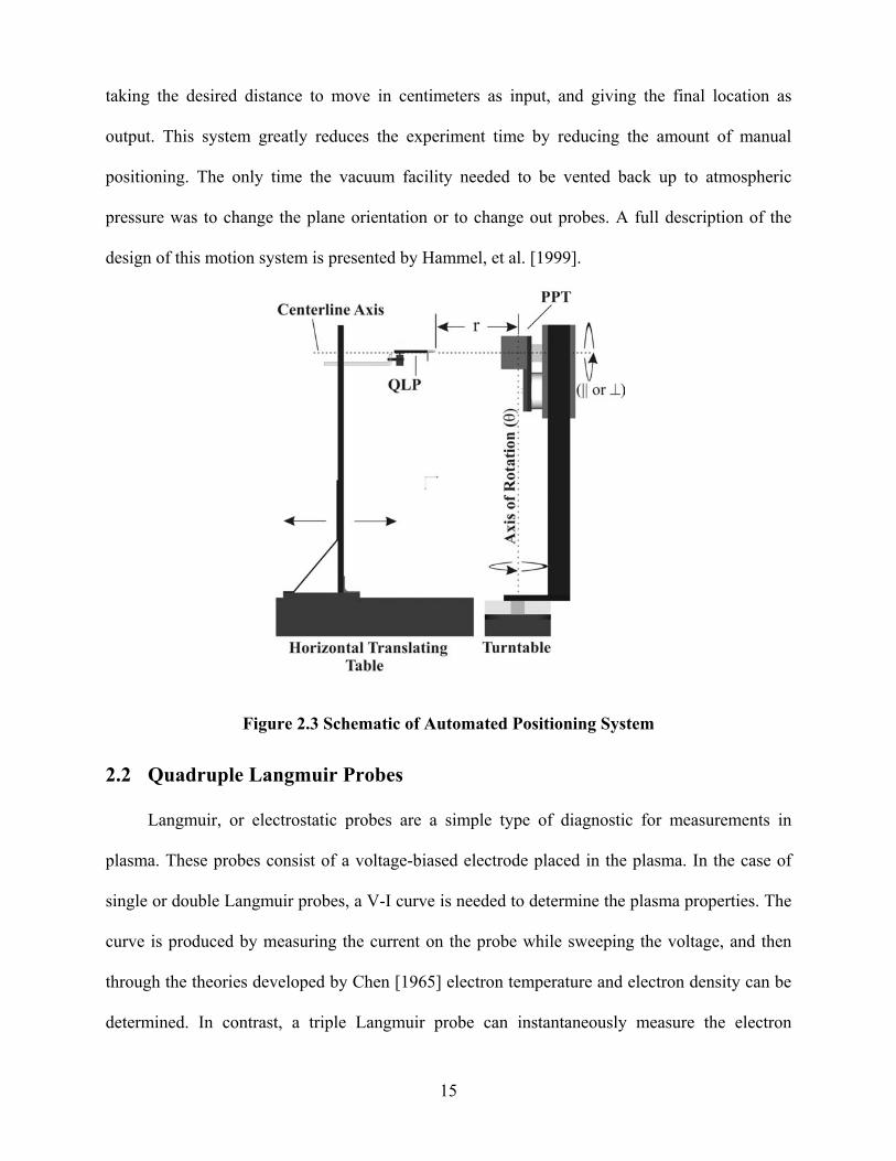
taking the desired distance to move in centimeters as input, and giving the final location as

output. This system greatly reduces the experiment time by reducing the amount of manual

positioning. The only time the vacuum facility needed to be vented back up to atmospheric

pressure was to change the plane orientation or to change out probes. A full description of the

design of this motion system is presented by Hammel, et al. [1999].

Figure 2.3 Schematic of Automated Positioning System

2.2 Quadruple Langmuir Probes

Langmuir, or electrostatic probes are a simple type of diagnostic for measurements in

plasma. These probes consist of a voltage-biased electrode placed in the plasma. In the case of

single or double Langmuir probes, a V-I curve is needed to determine the plasma properties. The

curve is produced by measuring the current on the probe while sweeping the voltage, and then

through the theories developed by Chen [1965] electron temperature and electron density can be

determined. In contrast, a triple Langmuir probe can instantaneously measure the electron

15

temperature and density. With the inclusion of a crossed electrostatic probe to a triple probe, it is

possible to not only measure electron temperature and density, but to measure the ion speed ratio

as well. The theory of the quadruple Langmuir probe is explained in the next section.

2.2.1 Quadruple Langmuir Probe Theory

The theory of operation of a quadruple Langmuir probe is a mixture of triple Langmuir

probe and crossed electrostatic probe theories, enabling the simultaneous measurement of

electron temperatureT t and density n t , and the ratio of ion flow velocity to the most

probable thermal speed S u . The triple probe theory was first derived from Chen and

Sekiguchi in 1965.

( )e ( )e

(

/i i= ic

A symmetrical triple Langmuir probe, like the one in Eckman, et al. [2001], is

comprised of three identical electrodes (P1, P2, P3) placed in parallel with the plasma flow vector.

As explained in Byrne, et al. [2001], a voltage mode of operation is one in which P2 is allowed to

float in the plasma and a fixed voltage )13 t

12( )t

(

φ is applied between the positive P1 and the negative

P3. The resulting voltage difference φ and collected current I allow for the iterative

evaluation of T t and n t . For a quadruple probe, the crossed, fourth electrode P

3( )t

( )e

14φ

( )e 4 has a

voltage bias applied to it that is equal to φ which allows for the evaluation of S . An

electrical diagram for the voltage mode operation of a QLP can be seen in Figure 2.4. However,

the PPT emits detectable amounts of EMI noise during the capacitor discharge and is not steady

state. As a result it has been shown that

13 i

)12 tφ is susceptible to measurement noise [Byrne, et al.

2001] in the voltage mode of operation. In light of this, the current mode TLP theory used by

Byrne, et al. [2001] has been expanded for the QLP. This theory has been previously outlined by

Gatsonis, et al. [2002]. In the new current mode, the quadruple probe has all of its electrodes

biased to the reference electrode P1. is a lesser potential difference than φ and φ , as can 12φ 13 14

16

be seen in Figure 2.5. All four probe currents are measured, and then four equations are solved

simultaneously for the values T t , , , and S . ( )e ( )en t 1sφ i

V 1

V 3 V

V 2

V f

0

V

4

P2

12

, ,ee eλ ,iiλ λ

, ,iλ λ

i

A

n

,e enλ in

− −

φ s

φ 3

φ 2

φ f

φ 1

φ

φ13 φ14

P1

P4P3

φ

φ12

Figure 2.4 Voltage Mode QLP Circuit

V 1

V 3 V 4

V 2

V f

0

V

φ s

φ 3

φ 2

φ f

φ 1

φ

φ13 φ14

φ12P1

P4P3

P2

Figure 2.5 Current Mode QLP Circuit

The assumptions for the quadruple probe analysis are as follows:

• The probe radius is much smaller than the mean free path of charged particle to

charged particle and charged particle to neutral particle collisions, therefore the

probe operates in the collisionless plasma regime,

i.e r ,p ei nλ λ

• The Debye length is much smaller than the probe radius, therefore the sheath is

collisionless, d . ,s e e iiλ λ

• The sheath thickness is smaller than the probe spacing, d s . s <

• The probe potential is less than the space potential for all probes, φ φ . p s≤

• The parallel probes have equal current collecting areas, A A . 1 2 3 4A A= = = ≡

• Current conservation applies, I I . 1 2 3 4 0I I− =

17

The current to a probe is classically defined as

. (2.1) p epI I I= − ip

)

The electron or retarded current is assumed to be positive, and the ion or accelerated current is

assumed to be negative. Therefore, for I the magnitude of the collected electron current is

larger than the magnitude of the collected ion current.

0p >

For a probe potential less than the space potential ( the electron current to the

probes parallel to the flow vector is given by

p sφ φ≤

( )exp exp spe p eo s p p eo

e e

eeI A J A JkT kT

φφ φ

= − − = −

(2.2)

where

12

2e

eo ee

kTnmπ

= J e is the electron current density from the thermal diffusion of electrons

to the sheath edge.

Ion current is dependent upon the operational regime of the probe as given by the Debye

ratio p Dλr , ion speed ratio S , the temperature ratio i i iTeT Z and the non-dimensional potential

( )p s peχ φ φ= − ekT (2.3)

The Debye length, assuming n , is i en≅

20D ekT e nλ ε= i (2.4)

For Debye ratios 5 , and 100p Dr λ≤ ≤ 3pχ > 1e i iT ≤T Z Petersen and Talbot [1970] give

the ion current to a probe parallel to the flow vector by an algebraic fit to Laframboise data as

(0i p iI A J αβ χ= + ) , (2.5)

where

18

1 2

0 2i e

i i ii

Z kTJ n Z eMπ

= . (2.6)

The parameters α and are defined as β

( )

0.752.9 0.07 0.34

ln 2.3i

i ep D

TZTr

αλ

= + − + (2.7)

( ) ( ) 3

1.5 0.85 0.135 lni i e p DT ZT rβ λ = + + (2.8)

The current collected by the probe perpendicular to the plasma flow vector is based on the theory

developed by Kanal [1964]. The electron current is defined as

exp spe p eo

e

eJ A J

kTφ = −

(2.9)

The ion current to the perpendicular probe is given by Kanal [1964] as a function of the speed

ratio , the non-dimensional potential of the probe, and the collection area. By assuming

negligible sheath thickness

iS

1s p →d r , Johnson and Murphree [1969] developed the expression

( ) ( )1 2

2

0

2 3exp !2 2

nei e i i

ne

kTI A n e S S n nmπ π

∞

⊥ ⊥=

= − Γ + ∑

e

. (2.10)

By applying the above assumptions and equations, and assuming T and Z the

following system of equations is arrived at for the quadruple probe:

i T= 1i =

( ) ( )

( ) ( )

1 11 0 0

1 12 1 122 0 0

1 13 1 133 0 0

4

exp

exp

exp

s se i

e e

s se i

e e

s se i

e e

e

e eI AJ AJkT kT

e eI AJ AJ

kT kT

e eI AJ AJ

kT kT

I A J

α

α

α

φ φβ

φ φ φ φβ

φ φ φ φβ

⊥

− = − + − + + = − + − + + = − +

=( ) ( )

122

1 14 20

0

2 3exp exp2 !

s e ie i

ne e

e kT SA n e S nkT m nφ φ

π π

∞

⊥=

− + − − + ∑ 2Γ

(2.11)

19

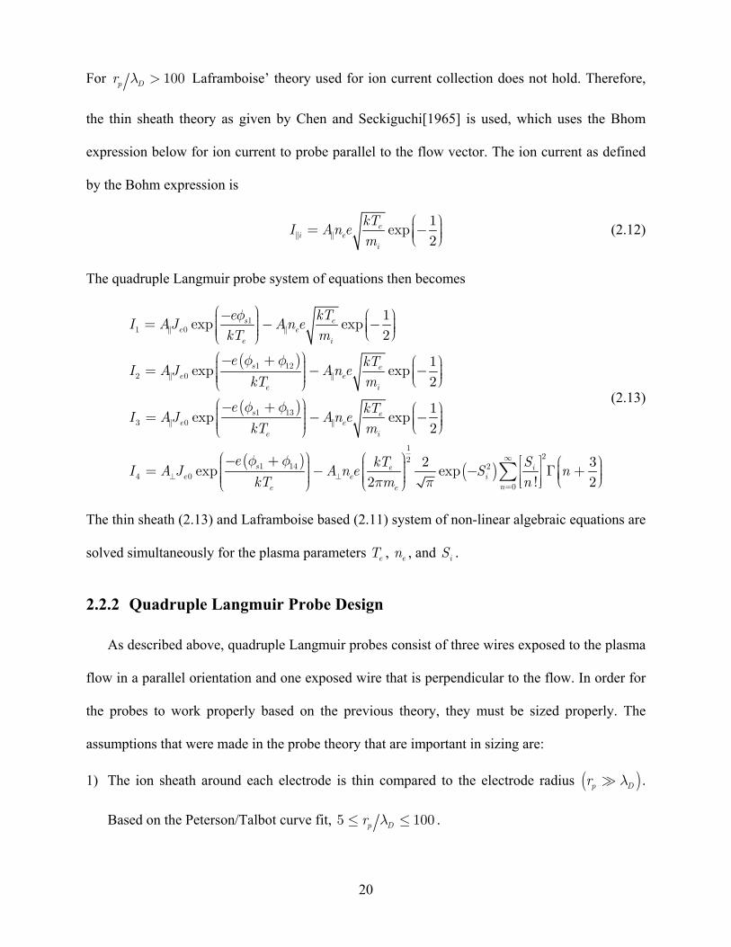
For 100p Dr λ > Laframboise’ theory used for ion current collection does not hold. Therefore,

the thin sheath theory as given by Chen and Seckiguchi[1965] is used, which uses the Bhom

expression below for ion current to probe parallel to the flow vector. The ion current as defined

by the Bohm expression is

1exp2

ei e

i

kTI An em

= − (2.12)

The quadruple Langmuir probe system of equations then becomes

( )

( )

11 0

1 122 0

1 133 0

14 0

1exp exp2

1exp exp2

1exp exp2

exp

s ee e

e i

s ee e

e i

s ee e

e i

se

e kTI AJ An ekT m

e kTI AJ An ekT m

e kTI AJ An ekT m

eI A J

φ

φ φ

φ φ

φ φ⊥

− = − − − + = − − − + = − −

− +=

( ) ( )1

2214 2

0

2 3exp2 !

e ie i

ne e

kT SA n e S nkT m nπ π

∞

⊥=

− − + ∑ 2

Γ

(2.13)

The thin sheath (2.13) and Laframboise based (2.11) system of non-linear algebraic equations are

solved simultaneously for the plasma parameters T , n , and S . e e i

2.2.2 Quadruple Langmuir Probe Design

As described above, quadruple Langmuir probes consist of three wires exposed to the plasma

flow in a parallel orientation and one exposed wire that is perpendicular to the flow. In order for

the probes to work properly based on the previous theory, they must be sized properly. The

assumptions that were made in the probe theory that are important in sizing are:

1) The ion sheath around each electrode is thin compared to the electrode radius ( ).

Based on the Peterson/Talbot curve fit,

p Dr λ

5 . 100p Dr λ≤ ≤

20

2) There must be free molecular flow in the sheath area of the electrodes, thus the Knudsen

number prλ=Kn should be much greater than one for ion-ion and ion-electron collisions.

3) The thin sheath approximation must hold, so λ and λ λ . ii Dλ ie D

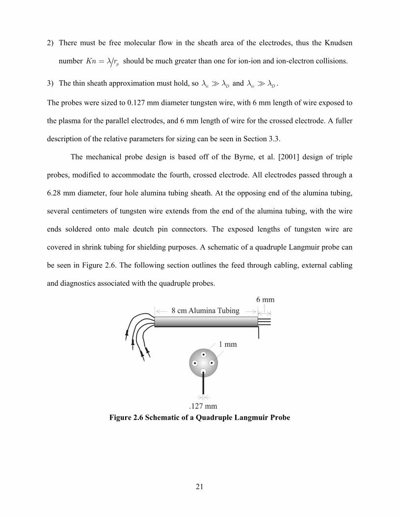
The probes were sized to 0.127 mm diameter tungsten wire, with 6 mm length of wire exposed to

the plasma for the parallel electrodes, and 6 mm length of wire for the crossed electrode. A fuller

description of the relative parameters for sizing can be seen in Section 3.3.

The mechanical probe design is based off of the Byrne, et al. [2001] design of triple

probes, modified to accommodate the fourth, crossed electrode. All electrodes passed through a

6.28 mm diameter, four hole alumina tubing sheath. At the opposing end of the alumina tubing,

several centimeters of tungsten wire extends from the end of the alumina tubing, with the wire

ends soldered onto male deutch pin connectors. The exposed lengths of tungsten wire are

covered in shrink tubing for shielding purposes. A schematic of a quadruple Langmuir probe can

be seen in Figure 2.6. The following section outlines the feed through cabling, external cabling

and diagnostics associated with the quadruple probes.

Figure 2.6 Schematic of a Quadruple Langmuir Probe

21

2.2.3 Cabling and Diagnostics

Each female deutch pin on the back of the quadruple probe is connected to the center

wire of a BNC coaxial cable. The BNC cables are individually covered with braided steal

shielding, and passed through the vacuum facility wall at an isolated BNC feed through. All

cables inside of the tank are the same length, and are laid out along Kapton shielding that has

been placed along the tank wall. On the outside of the tank, the shielded cables are connected to

BNC feedthroughs on a faraday cage. The faraday cage houses the PPT high voltage power

supply, triggering power supply, oscilloscope, probe biasing voltage sources, and the current

probes. The cable shielding and faraday cage were in place from previous efforts to take voltage

measurements in the PPT plume with TLPs [Byrne, et al., 2001].

Within the faraday cage, the probe signal wires were connected to the QLP circuitry as

shown in Figure 2.7. This circuitry is based on the previously described current-only QLP

theory. Voltages φ and φ are each supplied by two 9 volt batteries in series, and is

supplied by two 1.5 volt batteries in series. Voltage was measured after each shot throughout a

day of data acquisition, and the voltage was found not to change more than ±0.01 volts for every

100 data points collected. The voltages were measured before and after each glow cleaning, with

ranging from 2.876 to 2.989, and and φ ranging from 18.59 to 18.64 during the entire

data collection period. Currents I , , and I were each measured with a Tektronix model

TCP202 15 Ampere AC/DC current probe. These currents, as well as the discharge current, were

measured on a Tektronix model TDS3000 four channel oscilloscope, and copied to floppy disk

for transferal to a data reduction program on a PC.

13 14 12φ

12φ 13φ

3I

14

42

22

+-

Discharge Power Supply0-2000V DC

Ignition Power Supply0-30V DC

Tektronix 4 ChannelDigital Oscilloscope

AC110V

V12

3V

Cur

rent

Pro

be 2

33.3 µF

Spark Plug embeddedin electrode.

Teflon Fuel

Shielding around probe wires.

Vacuum Facilty CW-19

Tank Wall

Faraday Cage

Quadruple Langmuir probes

+

UnisonIgnition Circuit C

urre

nt P

robe

3

V13

18V

Rogowski CoilIntegration Circuit

Rogowski Coil

CathodeAnode

Igniter TriggerSwitch

V1418V

Cur

rent

Pro

be 4

Figure 2.7 Electrical Diagram of Experimental Facility

2.3 Experimental Procedures

2.3.1 Probe Cleaning

Over the course of many firings, the Langmuir probes will acquire a black residue from

the Teflon plasma. There are concerns that this residue will inhibit the current measurements,

and therefore an effective cleaning procedure must be enforced. The glow cleaning method used

in the previous PPT Langmuir probe experiments [Eckman, et al. 2001, Byrne, et al. 2001] has

proven to be effective, and was adopted by this experiment.

Glow cleaning is achieved by producing an arc between the exposed tungsten probe

23

wires, and an electrode. This arc cleans off the residues left by the plasma. The electrode setup

used in this experiment is identical to that used by Byrne, et al. [2001], which is composed of a

1.5 by 7 cm steel sheet that is insulated from the probe mounting system. The electrode is

connected to an isolated feed through, which in turn can be connected to the high voltage power

supply in the faraday cage. In order to create an arc between the electrode and the probe tips, the

local pressure at the tips must be increased. An argon gas feed system that injects argon gas very

close to the probe tips achieves this pressure increase. The argon gas line is made of

nonconductive material, and connected to a feed through at the tank wall. The line is then

connected to a Nupro regulator valve and a needle valve, which are used to regulate the flow

rate. First, the high voltage power supply is shut off, and the thruster is disconnected from the

power supply. The probe cables are disconnected from the probe circuitry, and are all connected

in parallel to the positive lead from the high voltage power supply. The cleaning electrode is

connected to the negative lead. The high voltage is then set to 1000 V. The gate valves that

separate the vacuum chamber from the oil diffusion pumps are closed, and the argon gas feed

line is opened. When the pressure reaches 4.0x10-5 torr, the argon feed line is closed, and at

4.2x10-5 torr, the high voltage power supply is turned on, and the thruster spark plug is

discharged. The spark plug discharge starts the arc between the Langmuir probe tips and the

cleaning electrode. After 30 seconds of constant glowing, the high voltage power supply is

turned off, and the electronics are put back in their original configuration. The 30-second glow

time was established form the previous Langmuir probe investigations within the large vacuum

facility [Byrne, et al., 2001].

2.3.2 Data Sampling

Quadruple probe data were taken on the planes perpendicular and parallel to the thruster

24

electrodes. Measurements were taken at 50, 70, 90, 110, and 130 degrees at 10 and 15cm from

the Teflon fuel bar face, and at 50, 60, 70, 80, 90, 100, 110, 120, and 130 degrees at 20cm from

the Teflon face. The measurement points taken at each energy level in the two planes can be seen

in Figure 2.8 and Figure 2.9 below.

0є

50є60є

70є80є90є100є110є120є

130є

10 cm15 cm 20 cm

ThrusterHousing

AnodeCathode

Figure 2.8 Perpendicular Plane Points

0є

60є70є

80є90є100є110є120є

10 cm15 cm 20 cmElectrode

ThrusterHousing

50є130є

Figure 2.9 Parallel Plane Points

At the beginning and end of each data collection period, the thruster was aligned to 20

cm, 90 degrees. Every time the vacuum facility was vented to atmospheric pressure, an angular

template and two different metric measuring tools were used to check this location. The high

voltage power supply was then set to the proper voltage for the 20 Joule thruster energy level.

The relationship between power supply voltage and thruster energy level is given by:

2V E= C (2.14)

with C =33µF. Once the thruster energy level is set, the probe is moved to 10 cm, 50 degrees,

the chamber is pumped down again, and all the data at 10 cm is taken. Data is then taken at 15

cm, then 20 cm. This process is repeated for the 5 Joule and 40 Joule energy levels.

At each data point, the thruster was fired four times. The recording of the shot was

triggered by the rise in the discharge current, giving a common trigger to all points at specific

thruster energy. Each shot was recorded by the oscilloscope, which then took the average of

25

those 4 shots and displayed it as the representative data set for that location. The data sets were

saved onto floppy disk for later transferal to a computer. With data taken at three energy levels in

each of the two planes, a total of 114 data points were recorded for the quadruple Langmuir

probes.

26

3 Data Reduction, Analysis, and Results

Using the experimental setup, diagnostics and theory described in Chapter 2, quadruple

Langmuir probe measurements were taken in perpendicular and parallel planes of the plume of a

pulsed plasma thruster. Current traces were measured at 10, 15, and 20 cm from the Teflon fuel

bar face, at angles up to 40 degrees off of the centerline in the parallel and perpendicular planes

of the 5, 20 and 40 J energy levels. The current traces were then run through data processing

software. The procedure for the software is as follows:

• Eliminate data points with measured Langmuir probe currents below the sensitivity of

the current probes.

• Obtain , , and S from the numerical solution of equations (2.11) or (2.13). To

determine whether the thin sheath or Laframboise equations are used, an initial guess is

obtained from the thin sheath solution, and then the Debye ratio

eT en i

p Dλr is evaluated. For

the final solution of T , , and S , if e en i 100p Dλ ≤r then equations (2.13) are used, else

if 100p Dλr then equations (2.11) are used. >

• Obtain , , and from the uncertainties in equations (2.11) or (2.13). eT∆ en∆ iS∆

Outliers are then removed from the data sets through a regression analysis. This chapter outlines

each of these steps in the reduction of the data, the details the error analysis, and presents the

data results.

3.1 Current Sensitivity

The DC accuracy of the current probes is given by the manufacturer as ±3%, correctable to

±2% from 50mA to 5A and ±1% from 5A to 15A when the probes are properly calibrated

[Tektronix]. In order to ensure that the data that is reduced is within the sensitivity of the probes,

27

a routine in the data reduction software eliminates those data points that are below the probe

sensitivity. For each data set, the maximum value for each current is found, and then compared

to what value of current/div setting would be needed to best fit that current to the 5 divisions

used to display the probe currents on the oscilloscope. The minimum current sensitivity for each

probe current is then found by calculating 2% of full scale, where full scale =10 x current/div.

Then at each time step of the data the four probe currents are compared to their corresponding

minimum sensitivity. If any of the currents are below this minimum sensitivity cutoff value then

that time step is skipped. For example, if an 80mA max current was measured for I , then the

corresponding current/div setting would be 20mA/div, so the minimum current sensitivity is 2%

of 200mA, or 4mA. Therefore, the code would eliminate all current values of below 4mA.

2

2I

3.2 Data Reduction Algorithm

After the current sensitivity filter, the data processing software finds the numerical solution to

the either the system of equations (2.11) or (2.13). The algorithm used is one developed from the

Numerical Recipes in Fortran [1996], a simultaneous multi-equation solver based on the

Newton-Raphson method. The Newton-Raphson method works by finding the root of n

functions that encompass n variables. So in general terms, it is desired that;

(3.1)

where F is the vector of all the functions, and x is the vector of variables. In this study:

(3.2) ( ) (1, , , , , , 0n e e s i n n e e s iF T n S I f T n Sφ = − =)1φ

)where is the measured current of probe n, and is the right hand side of the

system of equations (2.11) or (2.13). The function

nI ( 1, , ,n e e s if T n Sφ

F can be expanded in Taylor series, and be

represented in matrix form as:

28

( ) ( ) ( 2F x x F x J x O xδ δ+ = + ⋅ + )δ (3.3)

By setting ( ) 0xδ+ =F x and ignoring any 2xδ or higher terms, a set of linear equations is

formed that can be solved for xδ :

( )J x F xδ⋅ = − (3.4)

where J is the Jacobian matrix and is evaluated numerically. The variable vector x is modified

in the following manner:

new oldx x δ= + x (3.5)

This process is iterated until both x and F converge to some set accuracy.

The Newton-Raphson method requires an initial guess for the system of variables, given

as T , n , , and S that is sufficiently close to the root, or else it may not converge. For this

study, the initial guess T was supplied by iteratively solving the thin sheath equation

0e

0e

01sφ

0i

0e

2

3

1 2 4

1 3 4

1

1

de

de

ekT

ekT

I I I eI I I e

φ

φ

−

−

− − −=− − −

. (3.6)

The T solution is then used to obtain the ion current density from 0e

( )

( )

3 20

3 20

0 3 21

1

d de

d de

ekT

eikT

I I eJAe

φ φ

φ φ

− −

− −

−=−

. (3.7)

The electron density n is then obtained from: 0e

12

ie

e

i

JnkTe em

−= (3.8)

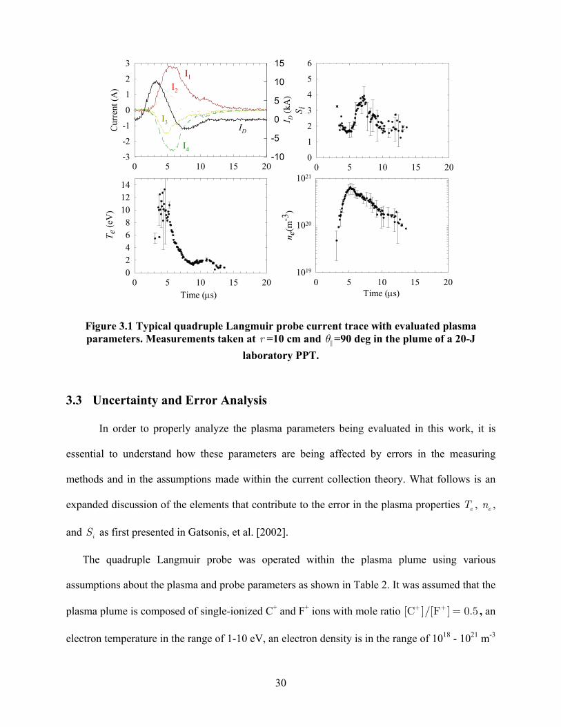
With T and , can be obtained by the solution of equation (4) in system (2.13), and

can be obtained by the solution of equation (1) in system (2.13). Figure 3.1 shows a typical

current trace and the resulting plasma properties.

0e

0en

0iS

01sφ

29

0 5 10 15 20

Cur

rent

(A)

-3

-2

-1

0

1

2

3

I D (k

A)

-10

-5

0

5

10

15

Time (µs)0 5 10 15 20

n e(m

-3)

1019

1020

10210 5 10 15 20

S i

0

1

2

3

4

5

6

Time (µs)0 5 10 15 20

T e (e

V)

02468

101214

I3

I4

ID

I1

I2

Figure 3.1 Typical quadruple Langmuir probe current trace with evaluated plasma parameters. Measurements taken at r =10 cm and θ =90 deg in the plume of a 20-J

laboratory PPT.

3.3 Uncertainty and Error Analysis

In order to properly analyze the plasma parameters being evaluated in this work, it is

essential to understand how these parameters are being affected by errors in the measuring

methods and in the assumptions made within the current collection theory. What follows is an

expanded discussion of the elements that contribute to the error in the plasma properties T , ,

and S as first presented in Gatsonis, et al. [2002].

e en

i

The quadruple Langmuir probe was operated within the plasma plume using various

assumptions about the plasma and probe parameters as shown in Table 2. It was assumed that the

plasma plume is composed of single-ionized C+ and F+ ions with mole ratio [C , an

electron temperature in the range of 1-10 eV, an electron density is in the range of 10

]/[F ] 0.5+ + =

18 - 1021 m-3

30

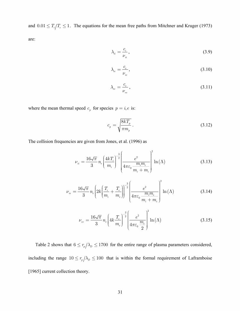
and 0.01 1i eT T≤ ≤ . The equations for the mean free paths from Mitchner and Kruger (1973)

are:

iii

ii

cλν

= , (3.9)

eie

ie

cλν

= , (3.10)

eee

ee

cλν

= , (3.11)

where the mean thermal speed c for species is: p ,p i= e

8 p

pp

kTc

mπ= . (3.12)

The collision frequencies are given from Jones, et al. (1996) as

( )

23

22

0

16 4 ln3 4

iii e i i

i

i i

kT en mmmm m

πνπε

− = Λ +

(3.13)

( )

23

22

0

16 23 4

i eie e i e

i e

i e

T T en k mmm mm m

πνπε

− = + Λ +

ln (3.14)

( )

2322

0

16 43 4

2

eee e e

e

T en k mmπν

πε

− = Λ ln (3.15)

Table 2 shows that 6 1700p Dr λ≤ ≤ for the entire range of plasma parameters considered,

including the range 10 that is within the formal requirement of Laframboise

[1965] current collection theory.

100p Dr λ≤ ≤

31

A relation for the sheath thickness needed to evaluate possible sheath interactions between

the probes is given by Liebmann, et al. [1994] as

( ) ( )342 3 2s D psd eλ φ= ekT . (3.16)

The maximum probe potential with respect to the plasma is expected on probe-3 and is estimated

to be between φ V. Table 2 shows that no interference is expected between the

sheaths since

3 25 60s −

31045 for the range of plasma parameters considered. 14ss d≤ ≤ ×

The other requirement for the application of the current-collection theory is that the probe

electrodes operate in the free-molecular regime, which implies 1st st prλ=Kn for all type of

collisions expected in the PPT plume. Charged-charged particle (e-i, i-i, e-e) and charged-

neutral particle (i-n, e-n) collisions affect the ion and electron currents collected by a probe in a

flowing plasma. There has been no theory that consistently accounts for collisional effects on

transitional probes although many studies have identified several effects as reviewed in Chung,

et al. [1974].

It is evident from Table 2 that the quadruple probe electrodes should operate for the most part

in the collisionless regime ( 1st st prλ= ≥Kn ). From the experiments it was found that the

probes were most often operating in the thin sheath regime, although in certain cases the

electrodes can be in the transitional regime. Ion-ion collisions in cases where account

for an increase in ion current. Bruce and Talbot [1975] measured an increase in the ion

(saturation) current of about of approximately 10% for an aligned probe with and

. Kirchoff, et al. [1971] showed that for λ λ or

1iiKn ≤

iiKn 0.08

10pχ = − 200ei D≥ ( D prλ )200ei ≥Kn electron-

ion collisions do not produce any transitional effects on the current with the probes in the

retarding region i.e. with probe potentials between plasma and floating. Kirchoff, et al. [1971]

32

also show that double-probes can be used for the determination of electron temperature even

when substantial collisional effects are present. Burton and Bushman [1999] offer a similar

explanation for quadruple probes.

Charged-neutral collisions reduce the current collected by a probe below it’s collisionless

limit predicted by Laframboise. Kirchoff, et al. [1971] discussed the effects of ion-neutral

collisions on the ion current for a probe in the ion-saturation regime and the effects of electron-

neutral collisions on the electron current for probes in the retarding-field regime. Table 2 shows

that the effects of ion-neutral and electron-neutral collision can be ignored.

Plasma Parameters Probe Parameters ne=1019 (m-3)

Te=2 eV, Ti=1 eV ne=1019 (m-3)

Te=5 eV, Ti=1 eV ne=1021 (m-3)

Te=2 eV, Ti=1 eV ne=1021 (m-3)

Te=5 eV, Ti=1 eV

p Dr λ 38.2 24.2 382.1 241.7

Ss d 300.9 190.3 3008.9 1903.0

,C CKn + + 3.3 11.5 0.044 0.15 ,F FKn + + 3.3 11.5 0.044 0.15 ,F CKn + + 3.1 10.9 0.041 0.14

,e CKn + 74.7 408.3 1 5.2 ,e FKn + 74.7 408.3 1 5.2

ei Dλ λ 2856.2 9868.0 376.5 1250.7

,e eKnτ

52.8 288.7 0.7 3.7 L 203.9 203.9 2039.3 2039.3

Neutral Parameters

nn = 1019(m-3)

n iT T= = .5 eV nn = 1019(m-3)

n iT T= = 1 eV nn = 1022(m-3)

n iT T= = 5 eV nn = 1022(m-3)

n iT T= = 1 eV

,C CKn + 2792.1 3948.6 2.8 3.9 ,F FKn + 4962.7 7016.9 5.0 7.0

,CEXC CKn + 589.7 2113.1 0.59 2.1

,CEXF FKn + 1574.3 5632.2 1.6 5.6

Table 2 Non-dimensional parameters of a quadruple probe with r m,

m in a PPT plume

41.25 10p−= ×

310s −=

The quadruple probe was aligned with the polar angle measured from the center of the

33

Teflon® surface which may have resulted in probe misalignment with the flow vector. These

issues have been discussed by Eckman, et al. [2001] where it was argued that the effects of

misalignment will not adversely affect triple probe measurements. The end-effects parameter

given by

12

1p eL

D i

L kT um

τλ

− = i (3.17)

is estimated in Table 2 using a maximum ion speed of u km/s. The fact that τ

ensures that end-effects are negligible, and therefore small misalignments of the probe that

would induce small changes in the collection area have no effect on the ion current.

30i = 50L

The uncertainties in T , , and S , designated as , , e en 1sφ i eT∆ en∆ 1sφ∆

2

3

4

and depend on

the propagation of uncertainties of all the parameters entering in their evaluation through the

system of equations (3.18). However, the system (3.18) is in implicit form, non-linear and

therefore uncertainly analysis is beyond the methodology presented in literature [Coleman and

Steel, 1999]. |The system (3.18) is in the form

iS∆

(3.18)

( )( )( )( )

1 1 1

2 1 12

3 1 13

4 1 14

, , , , , ,

, , , , , , ,

, , , , , , ,

, , , , , , ,

e e s i p p i

e e s i p p i

e e s i p p i

e e s i p p i

f T n S r l m I

f T n S r l m I

f T n S r l m I

f T n S r l m I

φ

φ φ

φ φ

φ φ

=

=

=

=

Upon differentiation the above system becomes

1 1 1 1 1 1 11 1

1

2 2 2 2 2 2 2 21 12 2

1 12

3

e e s i i p pe e s i i p p

e e s i i p pe e s i i p p

ee

f f f f f f fT n S m l r IT n S m l r

f f f f f f f fT n S m l rT n S m l r

f TT

φφ

φ φφ φ

∂ ∂ ∂ ∂ ∂ ∂ ∂ ∆ + ∆ + ∆ + ∆ = − ∆ + ∆ + ∆ +∆ ∂ ∂ ∂ ∂ ∂ ∂ ∂ ∂ ∂ ∂ ∂ ∂ ∂ ∂ ∂ ∆ + ∆ + ∆ + ∆ = − ∆ + ∆ + ∆ + ∆ +∆ ∂ ∂ ∂ ∂ ∂ ∂ ∂ ∂

∂ ∆ +∂

I

3 3 3 3 3 3 31 13 3

1 13

4 4 4 4 4 4 4 41 13 4

1 13

e s i i p pe s i i p p

e e s i i p pe e s i i p p

f f f f f f fn S m l rn S m l r

f f f f f f f fT n S m l rT n S m l r

φ φφ φ

φ φφ φ

∂ ∂ ∂ ∂ ∂ ∂ ∂ ∆ + ∆ + ∆ = − ∆ + ∆ + ∆ + ∆ +∆ ∂ ∂ ∂ ∂ ∂ ∂ ∂ ∂ ∂ ∂ ∂ ∂ ∂ ∂ ∂ ∆ + ∆ + ∆ + ∆ = − ∆ + ∆ + ∆ + ∆ +∆ ∂ ∂ ∂ ∂ ∂ ∂ ∂ ∂

I

I

(3.19)

34

The partial derivatives in the above system are the sensitivity coefficients and are obtained

analytically. The system (3.19) is solved numerically for , , and ∆

using the Newton-Raphson method. We proceed below with the evaluation of ∆ , , ,

, , , , , , and ∆ .

( )eT t∆ ( )en t∆ 1( )s tφ∆

1I

( )iS t

2 3I∆I∆

4I∆ pr∆ pl∆ 12φ∆ 13φ∆ 14φ∆ im

The uncertainties ∆ , ∆ , , and ∆ come from the TCP202 Tektronix current

probes used to measure the probe currents. ∆ , , , and are set equal to the

sensitivity values determined by the data processing software as described in section 3.1.

1I 2I 3I∆ 4I

1I 2I∆ 3I∆ 4I∆

From the TLP studies of Eckman [2000], it was found that the applied voltages varied

during the PPT discharge. Byrne, et al. [2001] eliminated the voltage variation by using

capacitors. However, it was found that the capacitors introduced a delay in the current

measurement and added non-plasma currents to the probes and were eliminated in Byrne, et al.

[2002] as well as in this investigation. The bias voltages were supplied from DC batteries. For

two 1.5V batteries were used in series and the applied and φ were each supplied by

two 9V batteries. To determine the variation of the applied voltages during the PPT discharge,

the voltage V of each quadruple Langmuir probe electrode was measured. The voltage

difference between the reference electrode V and the biased electrode V was then calculated.

Measurements were taken at 20cm downstream along the centerline for each bias voltage at each

energy level of 5J, 20J and 40J. The derived voltages φ , φ , and φ are shown in Figure 3.2,

Figure 3.3, and Figure 3.4 for the 5J, 20J, and 40J cases respectively. For the 5J data sets, Figure

3.2 shows there is no variation in the bias voltages φ , , and φ . In Figure 3.3 and Figure

3.4, does not vary greatly, but and φ both show a drop in value that corresponds to the

negative oscillation of the discharge current. Table 3 presents statistics for each voltage

measurement. The mean voltages during the pulse

12φ 13φ

13

14

14

p

1

14

p

12

12 13φ 14

12φ 13φ

12φ , 13φ , and 14φ for each energy level are

35

obtained by

11

1 ni

pin

φ=

= ∑ 1pφ . (3.20)

where φ is the i1ip

th voltage measurement in a measurement sample of n size.

The standard error about the mean is

( )1pssn

φ = (3.21)

where s, the standard deviation of the population, is given by

( )21 11

11

nip p

i

sn

φ φ=

= −− ∑ . (3.22)

The 95% confidence interval about the mean bias voltage was used as the random uncertainty for

the bias voltage, and is given as

( ) (1 ,p t z sφ ν∆ = ± )1pφ

)

(3.23)

where is the t-statistic for degrees of freedom, and z [SigmaPlot,

1997] . The values for

( ,t zν 1nν = − 1.96=

12φ∆ , 13φ∆ , and 14φ∆ are presented in Table 3. The mean voltages 12φ ,

13φ , and 14

e

φ are also used during the data processing routine during the solution for the plasma

parameters T , n , and . e iS

Discharge

Energy 12φ ( )12s φ 12φ∆ 13φ ( )13s φ

13φ∆

14φ ( )14s φ 14φ∆

E=5 J 3.396 .086 ±.169 19.166 .038 ±.075 18.672 .039 ±.077

E=20 J 3.117 .039 ±.076 18.982 .046 ±.091 17.958 .059 ±.115

E=40 J 3.390 .089 ±.175 18.078 .066 ±.130 17.269 .100 ±.196

Table 3 - Mean, standard error and random uncertainty for φ , φ , and φ 12 13 14

36

Time (µs)0 5 10 15 20

Vol

tage

(Vol

ts)

-60

-40

-20

0

20

40

Cur

rent

(kA

)

0

5

10

15

20

V1

Vp

IDC

φ1p

Time (µs)0 5 10 15 20

φ 12

(Vol

ts)

-4-202468

10

Time (µs)0 5 10 15 20

Vol

tage

(Vol

ts)

-60

-40

-20

0

20

40

Cur

rent

(kA

)

0

5

10

15

20

Time (µs)0 5 10 15 20

φ 13

(Vol

ts)

16171819202122

Time (µs)0 5 10 15 20

Vol

tage

(Vol

ts)

-60

-40

-20

0

20

40

Cur

rent

(kA

)

0

5

10

15

20

Time (µs)0 5 10 15 20

φ 14

(Vol

ts)

16171819202122

Figure 3.2 –Measurements of φ , φ , and φ taken at r =20 cm and =90 deg in the

plume of a 5 Joule laboratory PPT. 12 13 14 θ

37

Time (µs)0 5 10 15 20

Vol

tage

(Vol

ts)

-60-40-20

0204060

Cur

rent

(kA

)

-10

0

10

20

30

40

50

V1Vp

IDC

φ1p

Time (µs)0 5 10 15 20

φ 12

(Vol

ts)

0123456

Time (µs)0 5 10 15 20

Vol

tage

(Vol

ts)

-60-40-20

0204060

Cur

rent

(kA

)

-10

0

10

20

30

40

50

Time (µs)0 5 10 15 20

φ 13

(Vol

ts)

141618202224

Time (µs)0 5 10 15 20

Vol

tage

(Vol

ts)

-60-40-20

0204060

Cur

rent

(kA

)

-10

0

10

20

30

40

50

Time (µs)0 5 10 15 20

φ 14 (V

olts

)

1416

18202224

Figure 3.3 - Measurements of φ , , and φ taken at =20 cm and θ =90 deg in the

plume of a 20 Joule laboratory PPT. 12 13φ 14 r

38

Time (µs)0 5 10 15 20

Vol

tage

(Vol

ts)

-100

-50

0

50

100

Cur

rent

(kA

)

0

20

40

60

V1

Vp

IDC

φ1p

Time (µs)0 5 10 15 20

φ 12

(Vol

ts)

-4-202468

10

Time (µs)0 5 10 15 20

Vol

tage

(Vol

ts)

-100

-50

0

50

100

Cur

rent

(kA

)

0

20

40

60

Time (µs)0 5 10 15 20

φ 13

(Vol

ts)

12141618202224

Time (µs)0 5 10 15 20

Vol

tage

(Vol

ts)

-100

-50

0

50

100

Cur

rent

(kA

)

0

20

40

60

Time (µs)0 5 10 15 20

φ 14

(Vol

ts)

101214161820222426

Figure 3.4 - Measurements of φ , , and φ taken at =20 cm and θ =90 deg in the

plume of a 40 Joule laboratory PPT. 12 13φ 14 r

All electrode radii and lengths were measured using calipers with a precision of 0.0254

mm. The uncertainties ∆ and ∆ are both taken from the accuracy of the calipers used in the pr pl

39

construction of the probes as . ( ) ( ) 0.0254mmp pr t l t∆ = ∆ = ±

( )im t

( )T t ( )en t ( )iS t∆

pl∆ 12φ∆ 13φ∆ 14φ

The uncertainty in mass ∆ was set to zero due to the assumption in the current

collection theory that the plasma is comprised of singly ionized carbon and fluorine.

The right hand side of equation (3.19) contains the contributions to the errors ∆ ,

, and . The contributions of each term in the right hand side were analyzed

individually. The errors ∆ , ∆ , and were obtained from (3.19) with and

with , , , , ,

( )eT t

pr∆

( )en t∆

∆

( )iS t∆

2I 3I∆

e

4I∆

+

1I ∆ , , and all set to zero. The errors were then

evaluated with −∆ with all other right hand side terms again set to zero. This process was

repeated for each term in the right hand side. The resulting values of

pr

( )eT t∆ , ( )en t∆ ,

and ( )i∆S t are plotted in log scale in Figure 3.5 as absolute values. Included in Figure 3.5 are

the two plots of ( )eT t∆ , ( )en t∆ , and ( )iS t∆ where the right hand side terms are set to

positive values ( , , , pI+∆ pr+∆ pl+∆ 12φ+∆ , 13φ+∆ , and 14φ∆+ ), and all right hand side

terms set to negative values (−∆ , −∆ , −∆ , pI rp pl 12φ−∆ , 13φ−∆ , and 14φ−∆ ).

∆

Our analysis reveals that the dominant contributors to ( )eT t∆ are and I∆ 12φ∆ , all

other known uncertainties result in ( )eT t∆ magnitudes three orders of magnitude lower than

( )eT t∆ with all right hand side contributions included. The dominant contributor to ( )en t∆ is

, while has an effect on pr∆ nI∆ ( )en t∆ in the first 5 microseconds of the pulse. The dominant

contributors to ( )iS t∆ are ∆ and I 12φ∆ . Figure 3.5 shows that ( )eT t∆ , ( )en t∆ , and ( )iS t∆

have similar magnitudes regardless of the sign of the contributing uncertainty. Further effects of

sign can also be seen in Figure 3.6, which shows that when the sign of the uncertainties from the

right hand side of equation (3.19) are changed, then the sign of the errors also change. The error

40

( )eT t∆ has the same sign as and ∆ . can be maximized if the sign of ∆ is

opposite the sign of

12( )tφ∆ I ( )eT t∆ I

12φ∆

I

. A plot of this effect is included in Figure 3.6, where between 5 and 8

microseconds, the time period that corresponds to the peak currents collected by the probe

electrodes, an order of magnitude increase in can be seen due to the sign change of ∆ .

The error ∆ has the opposite sign of its major contributor ∆ . The magnitude of ∆

is increased when ∆ is of the opposite sign as ∆ . Through this analysis it was concluded

that the contribution of −∆ , , ,

( )eT t

pr

∆

pl

I

)( )en t pr (en t

I pr+∆ +∆ 12φ∆+ , 13φ+∆ , and 14φ∆+ will give the larger

errors of , , and ∆ . ( )eT t∆ (en t∆

pr∆

)

( )t

( )iS t

( ,e pr ±∆

(e t

)

r

)pr

)

( ,

( )

e pI

p ±( )pr t e )p

(en )t

12∆

pr∆

I

13

∆

0φ =p =

n ±∆

I l= ∆

( )en t

( )

φ = ∆

( ,e pr ±

n

( )en t (e

)p

)t

∆ r

In order to validate the error analysis, we evaluated whether the error ∆ would

encompass a solution of n t and n t respectively For the parameter

, solutions for n were found using r t . The resulting was

plotted against the solution for n with no modified parameters. Error bars for ∆ ,

evaluated with ± , and

(en t

e pr ±∆

)pI±∆

pr∆ ( ,n t

14φ = ∆

)pr

∆ were then placed around

. As seen in Figure 3.7 the values of n t fall within the error bars for n ,

thus showing that the error from predicts the plasma property n t . The

same process was followed with I t and produced the same results.

( ,e pr ±∆

41

.

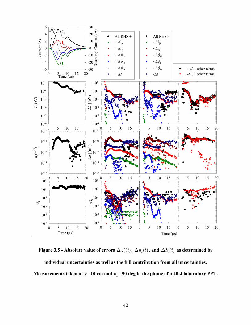
Time (µs)0 5 10 15 20

Cur

rent

(A)

-6

-4

-2

0

2

4

6

Dis

char

ge C

urre

nt (k

A)

-30

-20

-10

0

10

20

30

0 5 10 15

|∆n e|

(m-3

)

1017

1018

1019

1020

10210 5 10 15

|∆T e|

(eV

)

10-4

10-3

10-2

10-1

100

101

All RHS ++ ∆lp

+ ∆rp

+ ∆φ12

+ ∆φ13

+ ∆φ14

+ ∆I

Time (µs)0 5 10 15

|∆S i|

10-4

10-3

10-2

10-1

100

1010 5 10 15 20

0 5 10 15 20

0 5 10 15

All RHS -- ∆lp

- ∆rp

- ∆φ12

- ∆φ13

- ∆φ14

-∆I

0 5 10 15

0 5 10 15

0 5 10 15

T e (eV

)

10-4

10-3

10-2

10-1

100

101

0 5 10 15 20

n e(m-3

)

1017

1018

1019

1020

1021

Time (µs)0 5 10 15 20

S i

10-4

10-3

10-2

10-1

100

101

I1

I3

I4

DC

0 5 10 15 20

+∆I, - other terms-∆I, + other terms

I2

Figure 3.5 - Absolute value of errors , , and ∆ as determined by

individual uncertainties as well as the full contribution from all uncertainties.

Measurements taken at r =10 cm and θ =90 deg in the plume of a 40-J laboratory PPT.

( )eT t∆

⊥

( )en t∆ ( )iS t

42

0 5 10 15 20

∆ne(m

-3)

-1e+21

-5e+20

5e+20

1e+210 5 10 15 20

∆Te (

eV)

-2

-1

0

1

2

+∆rp,+∆lp,+∆I,+∆φ12,+∆φ13,+∆φ14

-∆rp,-∆lp,-∆I,-∆φ12,-∆φ13,-∆φ14

-∆I,+∆rp,+∆lp,+∆φ12,+∆φ13,+∆φ14

+∆I,-∆rp,-∆lp,-∆φ12,-∆φ13,-∆φ14

Time (µs)0 5 10 15 20

∆Si

-1

0

1

Figure 3.6 –Error for combination of uncertainties. Measurements taken at r =10 cm and

=90 deg in the plume of a 40-J laboratory PPT θ⊥

43

Time (µs)0 5 10 15 20

n e(m-3

)

1020

1021

ne(t)

blue bars=∆ne(t,-∆rp)

red bars=∆ne (t,+∆rp)ne(t,rp+∆rp) ne(t,rp-∆rp)

Time (µs)0 5 10 15 20

n e(m-3

)1020

1021

ne (t)blue bars=∆ne (t,-∆I)red bars=∆ne (+∆I)ne, (t,I+∆I)

ne, (t,Ip-∆I)

Figure 3.7 - Plot of n , n t , and n t . Measurements taken at r =10

cm and θ =90 deg in the plume of a 40-J laboratory PPT.

( )e t ( ),e p pr r±∆

⊥

( ,e I I±∆ )

3.4 Regression Analysis

During the first 2 to 5 microseconds of measured discharge current, there were data

points that resulted in very large values of electron temperature that fell well outside of the trends

in the data. In order to accurately detect the presence of outliers, a 4th or 6th degree polynomial

regression analysis was performed on the electron temperature for each set of reduced data

[SigmaPlot, 1997]. A plot of an initial regression can be seen in Figure 3.8. Each regression was

optimized to fit the trend of the data while achieving an R2 value as close to one as possible.

Once a regression was fit, any data points with standardized residuals above a value of two were

removed from the data set. A second regression was done on the modified set of data, as seen in

Figure 3.8. The second regression was used to check that the initial data removal improved the

curve fit of the data. If there were further data points with standardized residuals above 2 in

44

the second regression, then a second round of data point removal could be performed. In the case

of the data in Figure 3.8, the few points in the second regression with standardized residuals

above 2 were removed. The finalized set of data can be seen in Figure 3.9.

1st 4th degree Polynomial Regression

Time (µs)0 2 4 6 8 10 12 14

T e (eV

)

-10

0

10

20

30

40

50

60

70

Time (µs)

0 2 4 6 8 10 12 14

Stan

dard

ized

Res

idua

ls

-4-202468

10

R2=.411

2nd 4th degree Polynomial Regression

Time (µs)0 2 4 6 8 10 12 14

T e (eV

)-2

0

2

4

6

8

10

12

14

Time (µs)

0 2 4 6 8 10 12 14

Stan

dard

ized

Res

idua

ls

-4

-2

0

2

4

R2=.93

Figure 3.8 – Removal of outliers in T from the quadruple Langmuir probe data set at

=10 cm and θ =90 deg in the plume of a 20-J laboratory PPT. e

r

3.5 Quadruple Langmuir Probe Data Analysis

Typical quadruple Langmuir probe current traces and resulting plasma parameters are shown

in Figure 3.9. The typical discharge timescale is roughly 12 µs with a peak discharge at t .

The Langmuir probes start collecting currents at t µs, with probe-1 and probe-2 collecting

mostly electron current, while probe-2 and probe-4 collected mostly ion current. The current

3µs

2

45

collected by the probes last up until t µs, about 2 µs after the end of the discharge. Probe

current is measured in amperes, while discharge current is measured in kiloamperes. Figure 3.9

shows that there is an initial peak in electron current at the beginning of the pulse that points to

the presence of high temperature electrons associated with the peak of the discharge current.

Eckman, et al. [2001] noted similar findings. The electron temperature shows a secondary peak

occurs roughly 7 µs after the initial temperature peak, which has been observed in previous

investigations. The electron density peaks at t , roughly 2 µs after the peak discharge, and

ion speed ratio peaks at t , roughly 4µs after the peak discharge current. This section will

go over the data collected and the results taken from the analysis of all the current traces data.

14

5 sµ

7µ

10 15 20

DC

(kA

)

-10

-5

0

5

10

15n e

(m-3

)

10

10

10

S i

20

s

0 5

Cur

rent

(A)

-3

-2

-1

0

1

2

3

Time (µs)

0 5 10 15 2019

20

210 5 10 15 20

0

1

2

3

4

5

6I1

I2

I3

I4

DC

Time (µs)0 5 10 15

T e (e

V)

02468

101214

Figure 3.9 - Typical current trace with evaluated plasma parameters and error bars. Measurements taken at r =10 cm and θ =90 deg in the parallel plane of a 20-J laboratory

PPT.

3.5.1 Electron Density and Temperature of a PPT Plume

Figure 3.10, Figure 3.11, Figure 3.12, Figure 3.13, Figure 3.14, and Figure 3.15 show the

radial and angular variation of electron temperature, electron density and ion speed ratio on each

46

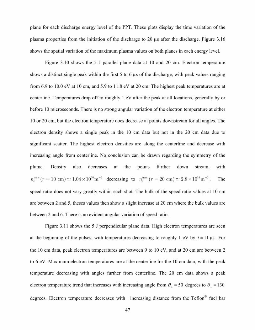
plane for each discharge energy level of the PPT. These plots display the time variation of the

plasma properties from the initiation of the discharge to 20 µs after the discharge. Figure 3.16

shows the spatial variation of the maximum plasma values on both planes in each energy level.

Figure 3.10 shows the 5 J parallel plane data at 10 and 20 cm. Electron temperature

shows a distinct single peak within the first 5 to 6 µs of the discharge, with peak values ranging

from 6.9 to 10.0 eV at 10 cm, and 5.9 to 11.8 eV at 20 cm. The highest peak temperatures are at

centerline. Temperatures drop off to roughly 1 eV after the peak at all locations, generally by or

before 10 microseconds. There is no strong angular variation of the electron temperature at either

10 or 20 cm, but the electron temperature does decrease at points downstream for all angles. The

electron density shows a single peak in the 10 cm data but not in the 20 cm data due to

significant scatter. The highest electron densities are along the centerline and decrease with

increasing angle from centerline. No conclusion can be drawn regarding the symmetry of the

plume. Density also decreases at the points further down stream, with

( )max 20 310 cm 1.04 10 men r −= × decreasing to ( )max 19 320 cm 2.8 10 me−= ×n r . The

speed ratio does not vary greatly within each shot. The bulk of the speed ratio values at 10 cm

are between 2 and 5, theses values then show a slight increase at 20 cm where the bulk values are

between 2 and 6. There is no evident angular variation of speed ratio.

Figure 3.11 shows the 5 J perpendicular plane data. High electron temperatures are seen

at the beginning of the pulses, with temperatures decreasing to roughly 1 eV by t . For

the 10 cm data, peak electron temperatures are between 9 to 10 eV, and at 20 cm are between 2

to 6 eV. Maximum electron temperatures are at the centerline for the 10 cm data, with the peak

temperature decreasing with angles further from centerline. The 20 cm data shows a peak

electron temperature trend that increases with increasing angle from

11 µs

50θ⊥ = degrees to 130θ⊥ =

degrees. Electron temperature decreases with increasing distance from the Teflon fuel bar

47

at all angles. The electron density shows a single peak over the length of the pulse, with peak

densities occurring at t . The highest electron densities are seen at centerline and then

decrease with increasing angles away from centerline. Bulk speed ratios at 10 cm are between 2

to 5, and at 20 cm are between 3 and 6. The 5 J perpendicular data follows most of the same

trends as the 5 J parallel data shown in Figure 3.10. Electron temperature increases with radial

distance from the Teflon fuel bar, though temperatures do not show large variation with change

in angle. At 10 cm, the parallel plane temperatures show equivalent bulk peak values, while at

20 cm the parallel plane data shows higher bulk peak temperature values at the beginning of the

pulses. Electron densities in both the parallel and perpendicular planes decrease with increasing

radial distance from the Teflon fuel bar and angles off centerline. The data at 10 cm in Figure

3.11 shows that the electron density variation with angular location may be asymmetric, as

electron densities do not decrease as rapidly from

9 µs

90θ⊥ = degrees to 130θ⊥ =

2010×

degrees as they

do in Figure 3.10. Bulk density values are similar for the two planes, between 1.5 m1810× -3 and

m201.0 10× -3 at 10 cm, and between 1.0 m1810× -3 and 3.0 m1910×

1810×

-3 at 20 cm. Speed ratios share

the same spatial variation trends in both planes, with similar bulk speed ratios.

Figure 3.12 shows the 20 J parallel plane data. High electron temperatures are seen in the

beginning of the pulse, with signs of a second, smaller temperature peak forming with 5 µs of the

first, as seen in the 10 cm data. Peak electron temperatures at 10 cm range between 8 to 12 eV.

Downstream at 20 cm, the peak temperatures range between 4 to 8 eV. Secondary electron

temperature peaks are not as evident in the 20 cm data. All temperature data decreases to roughly

1 eV after the reversal of the discharge current. Bulk electron densities range between 1.0

m-3 and 7.0 m-3 at 10 cm, and between m

1910×

2010× 2.5 -3 and m2.0 -3 at 20 cm. The

trends seen in the 5 J parallel plane data in Figure 3.10 are better defined in the 20 J data. The

48

electron density shows a single peak trend with maximum values occurring 3 to 4 µs after the

positive peak of the discharge current. The largest electron densities are at centerline, as in the 5

J data, and densities decrease symmetrically with angles off center, which concurs with the 5 J

parallel plane trends. Densities also decrease with increasing distance from the Teflon fuel bar,

as expected. Speed ratios show bulk values at 10 cm between 1.5 and 5 and between 2 and 6 at

20 cm. The 20 J, parallel plane spatial trends in speed ratio correspond to those seen in Figure

3.10, where the speed ratio does not vary greatly with angular variation, but the values do

increase with increasing distance downstream. There is however a trend for the bulk ion speed

ratios to increase from 1.5 to 3 as the angle increases from 50θ = degrees to 130θ = degrees.

Figure 3.12 shows evidence of the maximum speed ratio occurring about 3 µs after the positive

peak discharge current. This is not clearly seen in the 5 J data. Also, Figure 3.12 shows that the

20 J parallel plane peak electron temperatures are higher than the 5 J parallel plane electron

temperatures by 2 to 3 eV. Electron densities are higher in the 20 J data by an order of magnitude

as well.

Figure 3.13 shows the 20 J perpendicular plane data. All previously mentioned temporal

trends are evident: high electron temperatures at the beginning of the pulse, with a smaller

secondary peak in the 10 cm data shortly after the first and then a tapering off to roughly 1 eV,

density decreases asymmetrically with angular variation as well as at locations further

downstream, and ion speed ratio shows no large variation with angular variation, and increases at

locations downstream. The secondary peak is more defined in the 10 cm data of Figure 3.13 than

that of Figure 3.12.The bulk electron temperatures, electron densities and ion speed ratios are

equivalent between the two planes at 20 J. When compared to the 5 J perpendicular plane data in

Figure 3.11, it is evident that the maximum electron temperatures in Figure 3.13 are higher by 2

to 4 eV, and the electron densities are higher by an order of magnitude.

49

Figure 3.14 shows the 40 J parallel plane data. Previously noted trends apply: peak

electron temperatures are along the centerline, with decreasing temperatures downstream, high

temperatures are at the beginning of the pulse with evidence of a smaller secondary peak shortly

after the first, electron densities are at a maximum at centerline, and decrease symmetrically with

angular variation from centerline, electron density also decreases with increasing distance from

the Teflon fuel bar face, and ion speed ratios increase slightly with angular variation, and greatly

with increasing distance downstream. Peak electron temperatures at 10 cm are between 10 and

18 eV, while at 20 cm they are between 5 and 8 eV. Electron densities range from 1.0 m2010× -3

to 1.5 m2110× -3 at 10 cm, and 6.5 m1910× -3 to m206.0 10× -3 at 20 cm. Figure 3.14 shows that the

bulk electron temperatures are 1 to 2 eV higher and electron temperatures are up to an order of

magnitude larger than those in Figure 3.12, while bulk ion speed ratios are equivalent between

the 20 J and 40 J energy levels in the parallel plane.

Figure 3.15 shows the 40 J perpendicular plane data. Spatial and temporal trends follow

those as previously described, with the variation of electron density with angular variation being

asymmetric at 10 cm, the asymmetry is less evident at 20 cm. Bulk values of electron

temperature, electron density and ion speed ratio are the same as those in Figure 3.14. Figure

3.15 shows that in the 40 J perpendicular plane, the bulk values of electron temperature are 1 to 2

eV higher and the electron density is up to an order of magnitude greater than those seen in

Figure 3.13. Again, bulk values of speed ratio do not vary greatly between the 20 J and 40 J

perpendicular plane data.

The maxima of each data set are plotted in Figure 3.16 to better understand the spatial

variation of the plasma properties. The first column of plots shows the maxima for the 5 J data,

with the upper block showing the parallel plane data and the lower block showing the

perpendicular plane data. The next column is the 20 J data, in the same format, followed by the

50

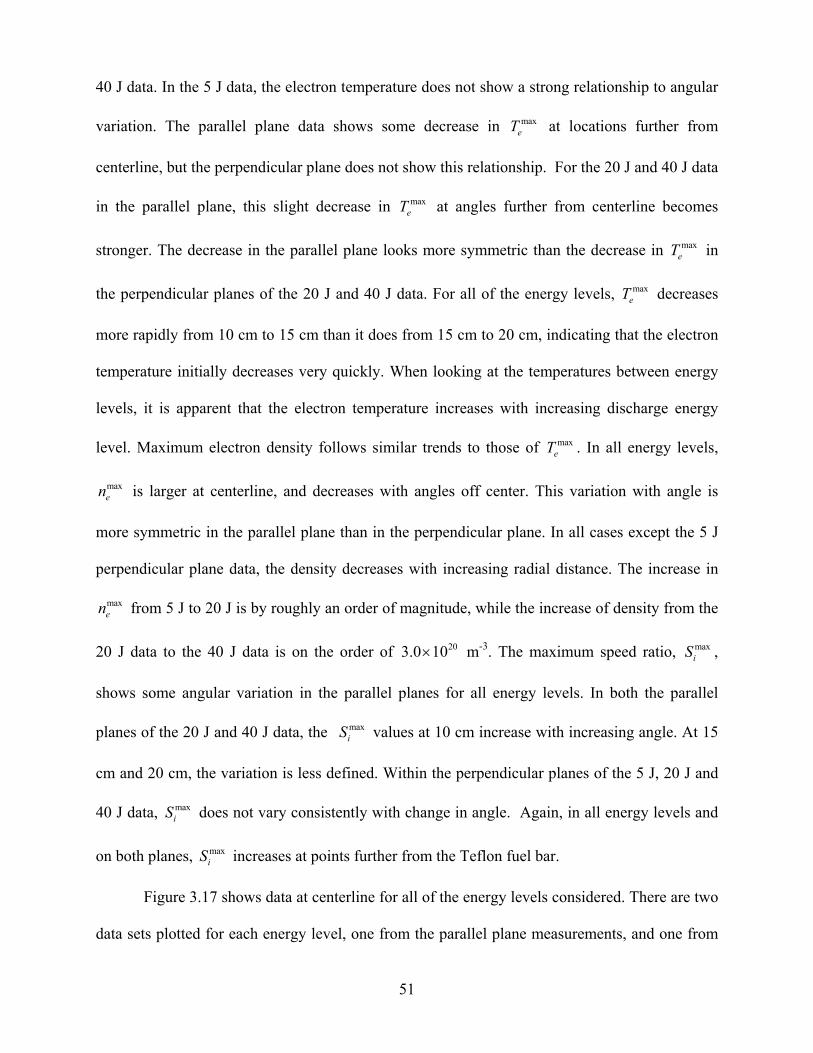
40 J data. In the 5 J data, the electron temperature does not show a strong relationship to angular

variation. The parallel plane data shows some decrease in T at locations further from

centerline, but the perpendicular plane does not show this relationship. For the 20 J and 40 J data

in the parallel plane, this slight decrease in at angles further from centerline becomes

stronger. The decrease in the parallel plane looks more symmetric than the decrease in T in

the perpendicular planes of the 20 J and 40 J data. For all of the energy levels, T decreases

more rapidly from 10 cm to 15 cm than it does from 15 cm to 20 cm, indicating that the electron

temperature initially decreases very quickly. When looking at the temperatures between energy

levels, it is apparent that the electron temperature increases with increasing discharge energy

level. Maximum electron density follows similar trends to those of T . In all energy levels,

is larger at centerline, and decreases with angles off center. This variation with angle is

more symmetric in the parallel plane than in the perpendicular plane. In all cases except the 5 J

perpendicular plane data, the density decreases with increasing radial distance. The increase in

from 5 J to 20 J is by roughly an order of magnitude, while the increase of density from the

20 J data to the 40 J data is on the order of 3.0 m

maxe

maxeT

×

maxe

maiS

maxe

maxe

maxen

maxen

2010 -3. The maximum speed ratio, ,

shows some angular variation in the parallel planes for all energy levels. In both the parallel

planes of the 20 J and 40 J data, the values at 10 cm increase with increasing angle. At 15

cm and 20 cm, the variation is less defined. Within the perpendicular planes of the 5 J, 20 J and

40 J data, does not vary consistently with change in angle. Again, in all energy levels and

on both planes, increases at points further from the Teflon fuel bar.

x

maxiS

maxiS

maxiS

Figure 3.17 shows data at centerline for all of the energy levels considered. There are two

data sets plotted for each energy level, one from the parallel plane measurements, and one from

51

the perpendicular plane measurements. As the centerline is the shared axis for the two planes, the

two sets of data can be compaired to see if there is substantial variation in the data between

shots. The magnitudes and data trends are almost the same between the two data sets at

centerline. It is concluded that the shot to shot variation in the data is minimal.

The following is a summary of the variations seen in electron temperature. There are high

values of electron temperature at the beginning of each pulse, with a smaller, secondary peak

becoming evident in the 20 J and 40 J energy levels. T then decreases to roughly 1 eV by the

end of the secondary peak of the discharge current. Electron temperature shows little variation

angularly in the parallel plane. Peak T values are at centerline for the parallel plane, with very

small decrease in maximum value towards the edges of the plume. In the 5 J, 20 J and 40 J

energy levels, T decreases with increasing distance downstream. The perpendicular plane shows

a non-symmetric angular variation of T in the 20 J and 40 J data, with peak values in the 20 J

data at 110 degrees, and a trend of temperate increase from 50 to 130 degrees in the 40 J data.

Bulk electron temperatures do not vary greatly from the parallel to the perpendicular plane in all

energy levels. Electron Temperatures increase with energy level, with the 20 J temperatures

between 2-4 eV higher than the 5 J temperatures, and the 40 J data 1-2 eV higher than the 20 J

temperatures.

e

e

e

e

Electron density can be summarized as having a single peak, usually 3 to 4 µs after the

main peak of the discharge current. Electron density shows distinct variation with radial and

angular variation, decreasing with angles off center and with movement of the plume

downstream. There is a more symmetric variation of electron density in the parallel plane than in

the perpendicular plane. The magnitudes of electron density between the perpendicular and

parallel planes of like energy levels are the same, but as energy level increases, so does the

electron density by an order of magnitude from 5 to 20 J, and by 3.0 m2010× -3 from 20 to 40 J.

52

The quadruple Langmuir probe electron temperature and density data from the 40 J

parallel plane are plotted in Figure 3.18 against triple Langmuir probe data from Byrne [2002].

The high temperature electrons are present in the beginning of the pulses for each of the data

sets, with the secondary temperature peak evident in both techniques at t . Trends in

electron density are similar in both techniques as well, with peak electron density of

, followed by a drop in electron temperature to

values below 2eV, and electron densities decline at the same rate for the two data sets. Spatial

relationships for the triple probe data show the same trends as those for the quadruple probe data

described above. This shows that the data produced from a current-mode quadruple Langmuir

probe technique closely matches data from a current-mode triple Langmuir probe technique.

10µ≅ s

( ) 20 310 cm, 90deg 1.5 10 men r θ −= = ×

53

n e (m

-3)

1018

1019

1020

1e+18

1e+19

1e+20

T e (eV

)

02468

10

Time (µs)0 5 10 15

Time (µs)0 5 10 15

Time (µs)0 5 10 15

S i

02468

Time (µs)0 5 10 15

Time (µs)0 5 10 15 20

r =10 cm θ|| =50 deg

I D (k

V)

-0.050.000.050.100.150.20 r =10 cm

θ|| =70 degr =10 cm θ|| =90 deg

r =10 cm θ|| =110 deg

r =10 cm θ|| =130 deg

n e (m

-3)

1018

1019

1020

1e+18

1e+19

1e+20

T e (eV

)

02468

10

Time (µs)0 5 10 15

Time (µs)0 5 10 15

Time (µs)0 5 10 15

S i

02468

Time (µs)0 5 10 15

Time (µs)0 5 10 15 20

r =20 cm θ|| =50 deg

I D (k

V)

-0.050.000.050.100.150.20 r =20 cm

θ|| =70 degr =20 cm θ|| =90 deg

r =20 cm θ|| =110 deg

r =20 cm θ|| =130 deg

Figure 3.10 Electron temperature, electron density and ion speed ratio from quadruple

probe measurements taken on the parallel plane of a 5-J laboratory PPT plume.

54

n e (m

-3)

1018

1019

1020

1e+18

1e+19

1e+20

T e (eV

)

02468

101214

Time (µs)0 5 10 15

Time (µs)0 5 10 15

Time (µs)0 5 10 15

S i

02468

Time (µs)0 5 10 15

Time (µs)0 5 10 15 20

r =10 cm θ⊥=50 deg

I D (k

V)

-0.050.000.050.100.150.20 r =10 cm

θ⊥ =70 degr =10 cm θ⊥ =90 deg

r =10 cm θ⊥ =110 deg

r =10 cm θ⊥=130 deg

No Data

No Data

No Data

n e (m

-3)

1018

1019

1020

T e (eV

)

02468

Time (µs)0 5 10 15

Time (µs)0 5 10 15

Time (µs)0 5 10 15

S i

0

2

4

6

Time (µs)0 5 10 15

Time (µs)0 5 10 15 20

r =20 cm θ⊥ =50 deg

I D (k

V)

-0.20.00.20.40.6 r =20 cm

θ⊥ =70 degr =20 cm θ⊥ =90 deg

r =20 cm θ⊥ =110 deg

r =20 cm θ⊥ =130 deg

Figure 3.11 Electron temperature, electron density and ion speed ratio from quadruple

probe measurements taken on the perpendicular plane of a 5-J laboratory PPT plume.

55

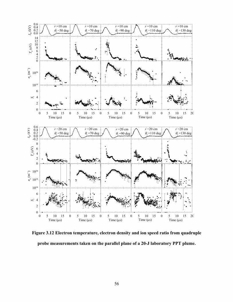
n e (m

-3)

1019

1020

1e+19

1e+20

1e+21

T e (eV

)

02468

101214

Time (µs)0 5 10 15

Time (µs)0 5 10 15

Time (µs)0 5 10 15

S i

0

2

4

6

Time (µs)0 5 10 15

Time (µs)0 5 10 15 20

r =10 cm θ|| =50 deg

I D (k

V)

0.00.20.40.6 r =10 cm

θ|| =70 degr =10 cm θ|| =90 deg

r =10 cm θ|| =110 deg

r =10 cm θ|| =130 deg

n e (m

-3)

1018

1019

1020

1e+18

1e+19

1e+20

1e+21

T e (eV

)

02468

Time (µs)0 5 10 15

Time (µs)0 5 10 15

Time (µs)0 5 10 15

S i

0

2

4

6

Time (µs)0 5 10 15

Time (µs)0 5 10 15 20

r =20 cm θ|| =50 deg

I D (k

V)

-0.20.00.20.40.6 r =20 cm

θ|| =70 degr =20 cm θ|| =90 deg

r =20 cm θ|| =110 deg

r =20 cm θ|| =130 deg

Figure 3.12 Electron temperature, electron density and ion speed ratio from quadruple

probe measurements taken on the parallel plane of a 20-J laboratory PPT plume.

56

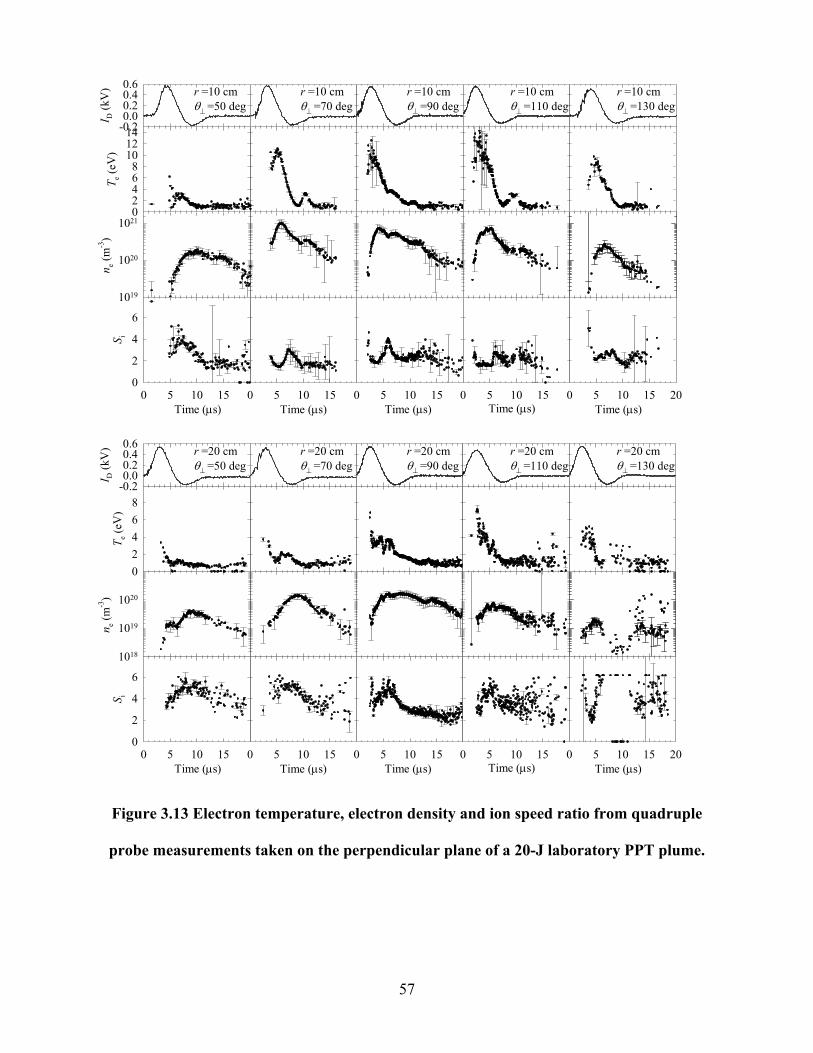
n e (m

-3)

1019

1020

1021

1e+19

1e+20

1e+21

T e (eV

)

02468

101214

Time (µs)0 5 10 15

Time (µs)0 5 10 15

Time (µs)0 5 10 15

S i

0

2

4

6

Time (µs)0 5 10 15

Time (µs)0 5 10 15 20

r =10 cm θ⊥ =50 deg

I D (k

V)

-0.20.00.20.40.6 r =10 cm

θ⊥ =70 degr =10 cm θ⊥ =90 deg

r =10 cm θ⊥ =110 deg

r =10 cm θ⊥ =130 deg

n e (m

-3)

1018

1019

1020

T e (eV

)

02468

Time (µs)0 5 10 15

Time (µs)0 5 10 15

Time (µs)0 5 10 15

S i

0

2

4

6

Time (µs)0 5 10 15

Time (µs)0 5 10 15 20

r =20 cm θ⊥ =50 deg

I D (k

V)

-0.20.00.20.40.6 r =20 cm

θ⊥ =70 degr =20 cm θ⊥ =90 deg

r =20 cm θ⊥ =110 deg

r =20 cm θ⊥ =130 deg

Figure 3.13 Electron temperature, electron density and ion speed ratio from quadruple

probe measurements taken on the perpendicular plane of a 20-J laboratory PPT plume.

57

n e (m

-3)

1018

1019

1020

1021

1e+18

1e+19

1e+20

1e+21

T e (eV

)

0

5

10

15

Time (µs)0 5 10 15

Time (µs)0 5 10 15

Time (µs)0 5 10 15

S i

02468

Time (µs)0 5 10 15

Time (µs)0 5 10 15 20

r =10 cm θ|| =50 deg

I D (k

V)

0.50.0

1.0 r =10 cm θ|| =70 deg

r =10 cm θ|| =90 deg

r =10 cm θ|| =110 deg

r =10 cm θ|| =130 deg

n e (m

-3)

1018

1019

1020

1021

1e+18

1e+19

1e+20

1e+21

T e (eV

)

0

5

10

15

Time (µs)0 5 10 15

Time (µs)0 5 10 15

Time (µs)0 5 10 15

S i

02468

Time (µs)0 5 10 15

Time (µs)0 5 10 15 20

r =20 cm θ|| =50 deg

I D (k

V)

0.50.0

1.0 r =20 cm θ|| =70 deg

r =20 cm θ|| =90 deg

r =20 cm θ|| =110 deg

r =20 cm θ|| =130 deg

Figure 3.14 Electron temperature, electron density and ion speed ratio from quadruple

probe measurements taken on the parallel plane of a 40-J laboratory PPT plume.

58

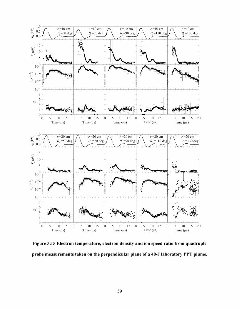
n e (m

-3)

1018

1019

1020

1021

1e+18

1e+19

1e+20

1e+21

T e (eV

)

0

5

10

15

Time (µs)0 5 10 15

Time (µs)0 5 10 15

Time (µs)0 5 10 15

S i

02468

Time (µs)0 5 10 15

Time (µs)0 5 10 15 20

r =10 cm θ|| =50 deg

I D (k

V)

0.50.0

1.0 r =10 cm θ|| =70 deg

r =10 cm θ|| =90 deg

r =10 cm θ|| =110 deg

r =10 cm θ|| =130 deg

n e (m

-3)

1018

1019

1020

1021

T e (eV

)

0

5

10

15

Time (µs)0 5 10 15

Time (µs)0 5 10 15

Time (µs)0 5 10 15

S i

02468

Time (µs)0 5 10 15

Time (µs)0 5 10 15 20

r =20 cm θ⊥ =50 deg

I D (k

V)

0.50.0

1.0 r =20 cm θ⊥ =70 deg

r =20 cm θ⊥ =90 deg

r =20 cm θ⊥ =110 deg

r =20 cm θ⊥ =130 deg

Figure 3.15 Electron temperature, electron density and ion speed ratio from quadruple

probe measurements taken on the perpendicular plane of a 40-J laboratory PPT plume.

59

T emax

(eV

)

05

10152025

n emax

(m-3

)

1018

1019

1020

1021

θ⊥ (degrees)

60 80 100 120

S imax

0

2

4

6

θ⊥ (degrees)

60 80 100 120

θ⊥ (degrees)

60 80 100 120

ED=5 J

T emax

(eV

)

05

10152025

ED=20 J ED=40 J

R=10cmR=15cmR=20cm

n emax

(m-3

)

1018

1019

1020

1021

θ|| (degrees)60 80 100 120

S imax

0

2

4

6

θ|| (degrees)60 80 100 120

θ|| (degrees)60 80 100 120

Figure 3.16 - Spatial variation of T , n , and in the plume of a laboratory model PPT.

maxe

maxe

maxiS

60

n e (m

-3)

1019

1020

1021

T e (eV

)02468

101214

Time (µs)0 5 10 15

Time (µs)0 5 10 15

Time (µs)0 5 10 15

S i

0

2

4

6

r =10 cm, θ =90E=5 J

I D (k

V)

0

1r =10 cm, θ =90Ε=20 J

r =10 cm, θ =90E=40 J

n e (m

-3)

1018

1019

1020

1021

1018

1019

1020

1021

T e (eV

)

02468

101214

Time (µs)0 5 10 15

S i

0

2

4

6

r =20 cm, θ =90E=5 J

I D (k

A)

0

1

Time (µs)0 5 10 15 20

r =20 cm, θ =90E=40 J

Time (µs)0 5 10 15

r =20 cm, θ =90E=20 J

Parallel Plane DataPerpendicular Plane Data

Figure 3.17 Discharge current, T at r =10 cm, r =20 cm and θ = 90 degrees in the

plume of a laboratory PPT operating at discharge energies of 5 J, 20 J, and 40 J. e en iS

61

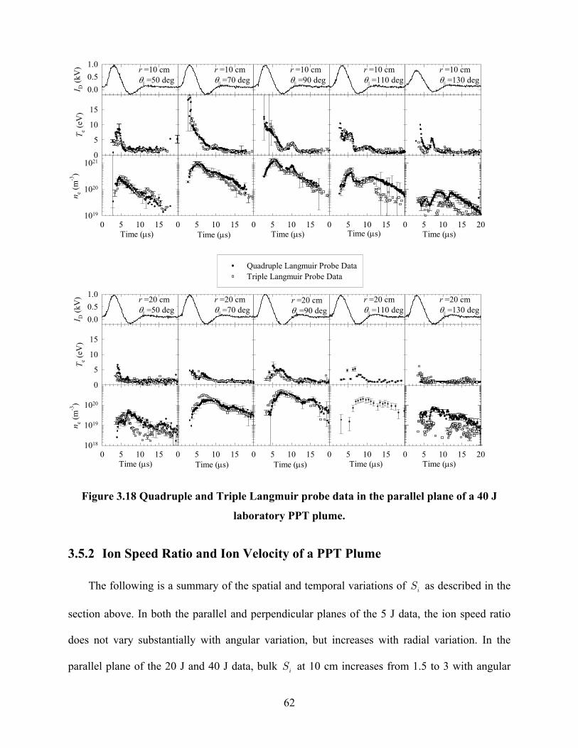
Time (µs)0 5 10 15

Time (µs)0 5 10 15

Time (µs)0 5 10 15

n e (m

-3)

1019

1020

1021

Time (µs)0 5 10 15

Time (µs)0 5 10 15 20

T e (eV

)

0

5

10

15

r =10 cm θ|| =50 deg

I D (k

V)

0.50.0

1.0 r =10 cm θ|| =70 deg

r =10 cm θ|| =90 deg

r =10 cm θ|| =110 deg

r =10 cm θ|| =130 deg

Time (µs)0 5 10 15

Time (µs)0 5 10 15

Time (µs)0 5 10 15

n e (m

-3)

1018

1019

1020

Time (µs)0 5 10 15

Time (µs)0 5 10 15 20

Quadruple Langmuir Probe DataTriple Langmuir Probe Data

T e (eV

)

0

5

10

15

r =20 cm θ|| =50 deg

I D (k

V)

0.50.0

1.0 r =20 cm θ|| =70 deg

r =20 cm θ|| =90 deg

r =20 cm θ|| =110 deg

r =20 cm θ|| =130 deg

Figure 3.18 Quadruple and Triple Langmuir probe data in the parallel plane of a 40 J

laboratory PPT plume.

3.5.2 Ion Speed Ratio and Ion Velocity of a PPT Plume

The following is a summary of the spatial and temporal variations of S as described in the

section above. In both the parallel and perpendicular planes of the 5 J data, the ion speed ratio

does not vary substantially with angular variation, but increases with radial variation. In the

parallel plane of the 20 J and 40 J data, bulk S at 10 cm increases from 1.5 to 3 with angular

i

i

62

variation. There are no strong angular variations in the perpendicular plane data of each energy

level. In both planes of each energy level, S increases with increasing distance downstream.

The bulk values of S at 10 cm for each plane fall between 1.5 . At 20 cm, the bulk

values of S are . For the 20 J case, S along the centerline increases from

i

i

3.5

4.5iS≤ ≤

i 6.0iS≤ ≤ i

( )maxiS r = 10 cm 3.9 to ( )max

i 20 cm 6.0=S r . For the 40 J case, S along the centerline

increases from

i

( )10 cmi =max 3.1S r to ( )m 5.4maxi

s t sµ µ

20 cS r . When looking at the

temporal variation of the speed ratio, it can been seen in Figure 3.10 through Figure 3.15 that

there is a peak in the value of at .

=

iS 6 8≤ ≤

ei i

i

kTm

u S=

Figure 3.19 shows the ion velocities during the time of a pulse as calculated from the

centerline values of electron temperature and speed ratio at the 5 J, 20 J and 40 J energy levels.

The ion velocities were evaluated from the definition of the speed ratio,

(3.24)

Peak evaluated ion velocities are between 35 km/s and 43 km/s at 5 J, 28 km/s and 30 km/s and

20 J, and between 33km/s and 37 km/s at 40 J. All peak values occur at the beginning of the

pulse. Signs of a secondary peak in ion speed are seen in the 10 cm data at the 20 J energy level,

and in the 10 cm and 15 cm data at the 40 J energy level. The peak ion speeds given by this

evaluation show good concurrence with previous ion speed studies.

63

E =20 cmθ|| =90 deg

u i (m/s)

10000

20000

30000

40000

50000

E=5 J θ|| =90 deg

10000

20000

30000

40000

50000

10 cm data15 cm data20 cm data

E =40 Jθ|| =90 deg

Time (µs)0 5 10 15 20

10000

20000

30000

40000

50000

Figure 3.19 Evaluated ion speeds at centerline in the plume of a laboratory PPT operating

at discharge energies of 5 J, 20 J, and 40 J.

64

4 Summary and Recommendations

4.1 Summary of Experimental Setup, Diagnostics and Procedures

Quadruple Langmuir probes were used to obtain electron density, electron temperature,

and ion speed ratio measurements in the plume of a NASA Glenn laboratory model pulsed

plasma thruster. This thesis documents a first attempt at using a quadruple Langmuir probe in the

unsteady plume of the PPT. The probe was used in a current-mode, where previous studies have

used the probe in a voltage-mode. The current collection theory was adapted to allow the

evaluation of plasma parameters in both the thin sheath and finite Debye length ratio regimes,

incorporating both thin sheath theory and the Laframboise corrections for finite Debye length

ratios.

A partially automated probe and thruster motion system was used to allow axial and

angular movement within a measurement plane. A glow discharge device was used to clean the

probes between firing sessions. The use of the automated motion system and the in-vacuum

probe cleaning system significantly decreased the time needed to aquire the necessary data. The

theory used for the evaluation of the plasma properties was reviewed and relevant plasma and

probe properties were calculated to ensure that the theory was applicable to the experiment, and

that all probes were designed to operate in the proper regime.

4.2 Summary of Data Reduction, Analysis and Results

Measurements were taken at 10, 15, and 20 cm from the face of the Teflon full bar, at

angles up to 40 degrees off of the centerline axis. Measurements were taken on planes parallel

and perpendicular to the thruster electrodes at discharge energy levels of 5 J, 20 J, and 40 J. A

65

data processing program was developed: it evaluated the plasma properties T , , and S ,

followed by the error in the plasma properties, ∆ , , and ∆ . Data outliers are removed

from the data sets using a regression method.

e en i

eT en∆ iS

Error analysis was performed. ∆ , , and were evaluated from a non-linear

system of error equations. Uncertainties in , , , , , and were

estimated. Error bars were determined from these evaluated uncertainties. It was concluded that

the largest source of error in electron density is due to ∆ and . The largest source of error

in electron temperature and ion speed ratio is due to and

eT en∆

I∆

iS∆

p ∆

pr

r∆

I∆

pl

φ

12φ∆

I∆

13φ∆ 14φ∆

12∆ .

4.2.1 Results and Discussion

Four current traces were taken at each of the locations mentioned above. These four

measurements are averaged to eliminate shot to shot variance and show the trend in the data over

time. Maxima are plotted for each energy level to better show the spatial variation of the data, as

well as to help analyze the expansion of the plasma plume.

In the 5 J case, electron temperatures range from 1 to 12 eV, electron densities range from

1.0x1018 m-3 to 1.5x1020 m-3, and ion speed ratio ranges from 1.8 to 6.05. For the 20 J case,

electron temperatures fall between 1 and 14 eV, electron densities are between 1.3x1018 m-3 to

1x1021 m-3, and the speed ratio ranges between 1.5 and 7.5. For the 40 J case, the bulk electron

temperature ranges between 1 to 20 eV, electron density is between 2x1018 m-3 and 1.2x1021 m-3,

with ion speed ratios between 1 and 6.09. For electron temperature and density, the largest values

fall along the centerline at the radius closest to the thruster and the smallest values were at the

outer edges of the measurement angles at 50 and 130 degrees. For ion speed ratio, the largest

values were at the edges of the plume in the far field measurement positions, with the smallest

values being on the centerline nearest the thruster.

66

There are two very defined spikes in electron temperature during the duration of the pulse,

especially in the higher operational energies of the thruster. The plume shows some asymmetry

in the perpendicular plane where the firing axis is oriented towards the anode of the thruster,

which is consistent with previous observations by Eckman [1999] and Arrington and Benson, et

al. [1999]. Ion speed ratio increases as the plume moves downstream, which is either due to the

ion temperature decreasing downstream, or as the plume expands, the ion velocity is increasing

downstream.

4.3 Recommendations

Recommendations are based on observations made during the experimentation process

and time spent in data analysis.

• Make voltage bias a time dependant value

Measuring the voltage biases on the probes would eliminate much of the error associated

with the bias voltage. This would require a electrical diagnostics setup that could measure

all four probe currents, the discharge current, and the voltage biases. This process would

require 8 oscilloscope channels for current and voltage measurements.

• Expand the measurement region

Taking many measurements along the radii could aid in quantifying the ion speed. Simple

time of flight analysis could be used as an initial guess for the ion speed, which would

help infer ion temperatures through the use of the ion speed ratio.

• Improve Current Measurement Resolution

Improving the minimum current that can be measured by the oscilloscope and/or current

probes would vastly improve the density of reducible data within a data point. The far

field 5 J data are plagued with low current measurements that are below the sensitivity of

67

the diagnostics, improving the sensitivity would solidify the observed trends in those data

points.

• Increase Number of Measurements at Individual Data Locations

Having a larger number of data points at single locations will allow for better statistical

analysis of the data to determine outliers and uncertainties. Also, each shot should be its

own data point, and all averaging should be done post data acquisition. This eliminates

the statistical data loss from using the oscilloscope to average the consecutive shots at a

data location.

68

References

Arrington, L.A., Benson, S., Hoskins, W., Meckel, N., “Development of a PPT for the EO-1 Spacecraft,” AIAA Paper 99-2276, June 1999.

Arrington, L.A. and Haag, T.W, “Multi-Axis Thrust Measurement of the EO-1 PPT,” AIAA

Paper 99-2290, June 1999. Arrington, L.A., Marrese C. M., and Blandino, J.J., “Pulsed Plasma Thruster Plume Study:

Symmetry and Impact on Spacecraft Surfaces,” AIAA Paper 2000-3262, July 2000. Bruce, C., Talbot, L., “Cylindrical Electrostatic Probes at Angles of Incidence,” AIAA Journal,

Vol. 13, No. 9, 1975, pp.1236-1238. Burton, R. L., Bufton, S. A., "Exit Plane Electrostatic Probe Measurements of a Low Power

Arcjet," Journal of Propulsion and Power, Vol. 12, No. 6, 1996. Burton, S. A., Bushman, S. S., “Probe Measurements in a Coaxial Gasdynamic PPT,” AIAA

Paper 99-2288, June 1999. Burton, R. L., DelMedico, S. G., Andrews, J. C., “Application of a quadruple Probe Technique

to MPD Thruster Plume Measurements,” Journal of Propulsion and Power, Vol. 9, No. 5, 1993.

Byrne, L., Gatsonis, N. A., Pencil, E., “Triple Langmuir Probe Measurements in the Plume and

Backflow Region of a Pulsed Plasma Thruster,” AIAA Paper 2001-3640, July 2001. Carter, J., Heminger, J., “Pulsed Plasma Thruster Contamination Studies,” Major Qualifying

Project ME-NAG-9503, Worcester Polytechnic Institute, February 1996. Chen, S., and Sekiguchi, T., "Instantaneous Direct-Display System of Plasma Parameters by

Means of Triple Probe", Journal of Applied Physics, Vol. 26, No 8, 1965, pp. 2363-2375. Chung, P. M., Talbot, L., Touryan, K. J., “Electric Probes in Stationary and Flowing Plasmas:

Part 1. Collisionless and Transitional Probes, and Part 2. Continuum Probes” AIAA Journal, Vol. 12, No. 2, 1974, pp. 133-154.

Coleman H.W. and Steele, W.G., Experimentation and Uncertainty Analysis for Engineers,

Wiley, 1999. Dawbarn, R., McGuire, R. L., Steely, S. L., Pipes, J. G., “Operating Characteristics on an

Ablative Pulsed Plasma Thruster,” Arnold Engineering Development Center TR-82-9, 1982.

Ebert, W.L., Kowal, S.J., Soan, R.F., “Operational Nova Spacecraft Teflon PPT System”, AIAA

Paper 89-2497, 1989.

69

Eckman, R. F., Byrne, L., Gatsonis, N. A., Pencil, E. J., “Triple Langmuir Probe Measurements

in the Plume of a Pulsed Plasma Thruster,” Journal of Propulsion and Power, Vol. 17, No. 4, 2001.

Gatsonis, N. A., Eckman R., Yin, X., Pencil, E. J., Myers, R. M., “Experimental Investigations

and Numerical Modeling of Pulsed Plasma Thruster Plumes,” Journal of Spacecraft and Rockets, Vol. 38, No. 3, pp. 454-464, 2001.

Gatsonis, N. A., Zwahlen, J. C., Wheelock, A., Pencil, E. J., Kamhawi, H., “Characterization of a

Pulsed Plasma Thruster Plume Using a Quadruple Langmuir Probe Method,” AIAA Paper 2002-4123, 2002.

Guman, W. J., and Begun, M., "Exhaust Plume Studies of a Pulsed Plasma Thruster", AIAA

Paper 97-704, April, 1978. Guman, W. J., and Nathanson, D. M., "Pulsed Plasma Microthruster Propulsion System for

Synchronous Orbit Satellite", Journal of Spacecraft and Rockets, Vol. 7, No. 4, April 1970, p. 409.

Hammel, J. R., Krumanaker, M. L., Zwahlen, J. C., “Design and Construction of an

Experimental Setup for Plasma Measurements in a Large Vacuum Facility”, Major Qualifying Project ME-NAG-9901, Worcester Polytechnic Institute, October, 1999.

Hirata, M., Murakami H., “Exhaust Gas Analysis of a Pulsed Plasma Engine”, AIAA Paper 84-

52, May, 1984. Johnson, B., Murphree, D., “Plasma Velocity Determination by Electrostatic Probes,” AIAA

Journal Vol. 7, No. 10, October 1969, pp. 2028-2030. Jones, M. E., Lemons, D. S., Mason, R. J., Thomas, V. A., Winske, D., “A Grid-Based Coulomb

Method for PIC Codes,” Journal of Computational Physics, Vol. 123, No. 1, 1996, pp. 169-181.

Kanal, M., “Theory of Current Collection of Moving Cylindrical Probes,” Journal of Applied

Physics, Vol. 35, No. 6, June 1964, pp. 1697-1703. Kirchoff, R. H., Peterson, E. W., Talbot, L., “An Experimental Study of the Cylindrical

Langmuir Probe Response in the Transition Regime,” AIAA Journal, Vol. 9, No. 9, 1971, pp. 1686-1694.

Laframboise, J., “Theory of Cylindrical and Spherical Langmuir Probes in a Collisionless

Plasma at Rest,” UTIAS Rept. 100, June 1966. Lam, S. H., “Unified Theory for the Langmuir Probe in a Collisionless Plasma,” The Physics of

Fluids, Vol. 8, No. 1, 1965, pp 73-87. Mitchner, M., Kruger, Jr., C. H., Partially Ionized Gases, Stanford University, 1973.

70

Myers, R. M., Oleson, S. R., Curran, F. M., Schneider, S. J., ”Small Satellite Propulsion Options”, 29th Intersociety Energy Conversion Engineering Conference, Monterey, CA, Aug. 7-11, 1994, p. 744-749.

Myers, R. M., Oleson, S., McGuire, M., Meckel, N., and Cassady, R.J., "Pulsed Plasma Thruster

Technology for Small Satellite Missions", NASA CR 198427, November 1995. Myers, R. M., Arrington, L. A., Pencil, E. J., Carter, J., Heminger, J., Gatsonis, N. A., “Pulsed

Plasma Thruster Contamination", AIAA Paper 96-2729, July, 1996. Peterson, E. W. and Talbot, L., Collisionless Electrostatic Single-Probe and Double-Probe

Measurements, AIAA Journal, Vo. 8, No.12, 1970, pp.2215-2219. Poissant, G., Dudeck, M., “Velocity Profiles in a Rarafied Plasma Stream by Crossed

Electrostatic Probes,” Journal of Applied Physics, Vol. 58, No. 5, 1985, pp. 1772-1779. Pollard, J. E., Jackson, D. E., Marvin, D. C., Jenkin, A. B., Janson, S. W., “Electric Propulsion

Flight Experience and Technology Readiness,” 29th Joint Propulsion Conference and Exhibit, Monterey, CA, June 28-30, 1993.

Rudolph, L.K., Harstad, K.G., Pless, L.C., Jones, R.M., “Plume Characterization of a One-

Millipound Solid Teflon Pulsed Plasma Thruster”, Air Force Rocket Propulsion Laboratory TR-79-60, NASA CR-162786, Sept. 1979.

SigmaPlot Users Manual, SPSS Inc, 1997. Spanjers, G.G., Lotspeich, J.S., McFall, K.A., Spores, R.A., “Propellant losses Because of

Particulate Emission in a Pulsed Plasma Thruster,” Journal of Propulsion and Power, Vol.14, No.4, 1998,pp. 554-559.

Thomassen, K. I., and Vondra, R.J., "Exhaust Velocity Studies of a Solid Teflon Pulsed Plasma

Thruster", Journal of Spacecraft and Rockets, Vol. 9, No. 1, Jan. 1972, pp. 61-64. Thomassen, K. I., and Tong, G., "Interferometric Density Measurements in the Arc of a Pulsed

Plasma Thruster", Journal of Spacecraft and Rockets, Vol. 10, No. 3, March 1973, pp. 163-164.

Vondra, R. J., Thomassen, K., and Solbes, A., "Analysis of Solid Teflon Pulsed Plasma

Thruster", Journal of Spacecraft and Rockets, Vol. 7, No. 12, 1970, pp. 1402-1406.

71