investigation into the efficiency of a t foil

Investigation into the efficiency of a

T Foil

Student: Amelia Nunn

Student ID: 611022

Lecturer: Dev Ranmuthugala

Subject: Applied Computational Fluid Dynamics

Course: Bachelor of Engineering (Marine & Offshore Systems)

Due Date: 27th of April 2011

JEE480-Investigation into the efficiency of a T Foil 2011

2 Amelia Nunn

Abstract This paper investigates the computational results produced by varying the Angle of Attack and velocity

on a scaled T Foil using ANSYS 12.1 CFX. The CFD data was compared to 2008 and 2009 tank data to

analyse its accuracy and relativity to true data. The coefficient of lift was found to be at around 13 degrees

at the lowest velocity and 12.5 degrees for the higher velocities. The results found that the T Foil is at

maximum efficiency when operated at an Angle of Attack of 9 degrees. Figure 1 summarizes the results

of the present investigation.

A secondary mesh was produced to investigate the varying results when the mesh is refined from an

initial 500,000 elements to 2.3 million elements. The investigation focussed on analysing the T Foil at a 0

degree Angle of Attack at four different speeds. The refined mesh produced a higher lift, smaller drag and

reduced moment when compared to the coarse mesh.

Figure 1 Wing Characteristics at 2.1 m/s


3 Amelia Nunn

Contents

Abstract ........................................................................................................................................................ 2

Contents ....................................................................................................................................................... 3

Nomenclature .............................................................................................................................................. 5

Abbreviations .............................................................................................................................................. 6

List of Figures .............................................................................................................................................. 7

List of Tables ............................................................................................................................................... 8

2.0 Theory .............................................................................................................................................. 9

2.1 NACA Airfoils .............................................................................................................................. 9

2.2 Scaling......................................................................................................................................... 14

2.3 Turbulence model ....................................................................................................................... 14

3.0 Geometry ....................................................................................................................................... 15

3.1 NACA foils ................................................................................................................................. 15

3.2 Rhinoceros 4.0 Model ................................................................................................................. 16

3.3 Domain ........................................................................................................................................ 18

4.0 Mesh ............................................................................................................................................... 19

4.1 Grid Independence Study ............................................................................................................ 19

4.2 Analysis Mesh ............................................................................................................................. 19

4.3 Refined Mesh .............................................................................................................................. 24

5.0 Setup ............................................................................................................................................... 26

6.0 Results ............................................................................................................................................ 27

6.1 Analysis Mesh ............................................................................................................................. 27

6.1.1 CFD Data .......................................................................................................................................... 28

6.1.2 CFD Data Calculations ..................................................................................................................... 29

6.1.3 CFD Data vs Tank Data .................................................................................................................... 30

6.2 Refined Mesh .............................................................................................................................. 32

6.2.1 Refined Mesh vs Analysis Mesh ......................................................................................................... 32

7.0 Discussion....................................................................................................................................... 33

7.1 Grid Independence Study ............................................................................................................ 33

7.2 Convergence ............................................................................................................................... 33

7.3 Stall Angle and Separation .......................................................................................................... 34

7.4 Y+ ............................................................................................................................................... 36

7.5 Pressure Development................................................................................................................. 38


4 Amelia Nunn

7.6 Vortices Progress ........................................................................................................................ 40

7.7 Lift, Drag and Pitching Moment ................................................................................................. 42

7.8 Analysis Mesh CFD Data vs. Tank Data .................................................................................... 42

7.9 Analysis Mesh vs. Refined Mesh ................................................................................................ 42

8.0 Conclusion ..................................................................................................................................... 43

9.0 Recommendations ......................................................................................................................... 44

10.0 References ...................................................................................................................................... 45


5 Amelia Nunn

Nomenclature

α Angle of Attack ˚

b0012 Wing Span of the NACA 0012 foil mm

b0015 Wing Span of the NACA 0015 foil mm

c0012a Wing Chord of the NACA 0012 foil at the tip mm

c0012b Wing Chord of the NACA 0012 foil midway between the wing span mm

c0015 Wing Chord of the NACA 0015 foil mm

CD Drag Coefficient -

CL Lift Coefficient -

CM Pitching Moment Coefficient -

D Drag N

g Gravity [9.81ms-2

] ms2

L Lift N

M Pitching moment Nm

ρ Density of the fluid kg/m3

μ Fluid Dynamic Viscosity kg/ms

Re Reynold’s Number -

T(x) Thickness Distribution over foil m

S Wing Area m

V Speed ms1


6 Amelia Nunn

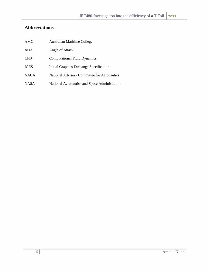
Abbreviations

AMC Australian Maritime College

AOA Angle of Attack

CFD Computational Fluid Dynamics

IGES Initial Graphics Exchange Specification

NACA National Advisory Committee for Aeronautics

NASA National Aeronautics and Space Administration


7 Amelia Nunn

List of Figures

Figure 1 Wing Characteristics at 2.1 m/s ...................................................................................................................... 2 Figure 2-1 NACA foil (US Department of Transportation, 1980) ................................................................................. 9 Figure 2-2 Forces on a NACA foil (US Department of Transportation, 1980) ........................................................... 10 Figure 2-3 Typical Wing Characteristics (Abbot & Doenhoff, 1959) ......................................................................... 11 Figure 2-4 Stall - Separation of an Airfoil (NASA, 2011) ........................................................................................... 12 Figure 2-5 Pressure Distribution about the foil .......................................................................................................... 13 Figure 2-6 Vortex pattern for a tapered wing (Graebel, 2007) ................................................................................... 13 Figure 3-1 NACA 0012a c=54mm ............................................................................................................................... 15 Figure 3-2 NACA 0012b c=75.6mm ............................................................................................................................ 15 Figure 3-3 NACA 0015 ................................................................................................................................................ 15 Figure 3-4 Perspective view of T Foil ......................................................................................................................... 16 Figure 3-5 Top View of T Foil ..................................................................................................................................... 16 Figure 3-6 Splits in Horizontal Foil ............................................................................................................................ 17 Figure 3-7 Splits in Strut ............................................................................................................................................. 17 Figure 3-8 Domain ...................................................................................................................................................... 18 Figure 4-1 Grid Independence Study........................................................................................................................... 19 Figure 4-2 Domain mesh at AOA 12 degrees .............................................................................................................. 20 Figure 4-3 Analysis Mesh about the T-Foil ................................................................................................................. 21 Figure 4-4 Splits through T-Foil ................................................................................................................................. 22 Figure 4-5 Inflated Boundary ...................................................................................................................................... 23 Figure 4-6 Refined Mesh – Domain ............................................................................................................................ 25 Figure 4-7 Refined Mesh ............................................................................................................................................. 25 Figure 5-1 Domain Setup ............................................................................................................................................ 26 Figure 6-1 Analysis Mesh – L vs AOA ......................................................................................................................... 28 Figure 6-2 Analysis Mesh – D vs AOA ....................................................................................................................... 28 Figure 6-3 Analysis Mesh – M vs AOA ........................................................................................................................ 28 Figure 6-4 Analysis Mesh - CL vs AOA ....................................................................................................................... 29 Figure 6-5 Analysis Mesh – CD vs AOA ....................................................................................................................... 29 Figure 6-6 Analysis Mesh – CD vs AOA ....................................................................................................................... 30 Figure 6-7 CD Vs CL - Tank Data vs CFD Data .......................................................................................................... 30 Figure 6-8 CD vs AOA - Tank Data vs CFD Data ....................................................................................................... 31 Figure 6-9 CL vs AOA - Tank Data vs CFD Data ....................................................................................................... 31 Figure 6-10 Refined Mesh vs Analysis Mesh ............................................................................................................... 32 Figure 7-1 Velocity Streamlines at AOA 0 degrees, velocity = 0.9m/s ........................................................................ 34 Figure 7-2 Velocity Streamlines at Stall (13 degrees), velocity 0.9 m/s ...................................................................... 35 Figure 7-3 Velocity Streamlines after Stall (16 degrees), v= 0.9 m/s.......................................................................... 35 Figure 7-4 Y+ AOA 0 degrees, v=0.9m/s ................................................................................................................... 36 Figure 7-5 Y+ AOA 16 degrees, v=4.4m/s .................................................................................................................. 37 Figure 7-6 Pressure @ AOA 0 degrees, v=0.9m/s ...................................................................................................... 38 Figure 7-7 Pressure @ AOA 13 degrees, v=0.9m/s .................................................................................................... 38 Figure 7-8 Pressure @ AOA 16 degrees, v=0.9m/s .................................................................................................... 39 Figure 7-9 Vortices @ AOA 0 degrees, v=0.9m/s ....................................................................................................... 40 Figure 7-10 Vortices @ AOA 13 degrees, v=0.9m/s ................................................................................................... 41 Figure 7-11 Vortices @ AOA 16 degrees, v=0.9m/s ................................................................................................... 41 Figure 7-12 Analysis Mesh – Lift/Drag vs Angle of Attack ......................................................................................... 42


8 Amelia Nunn

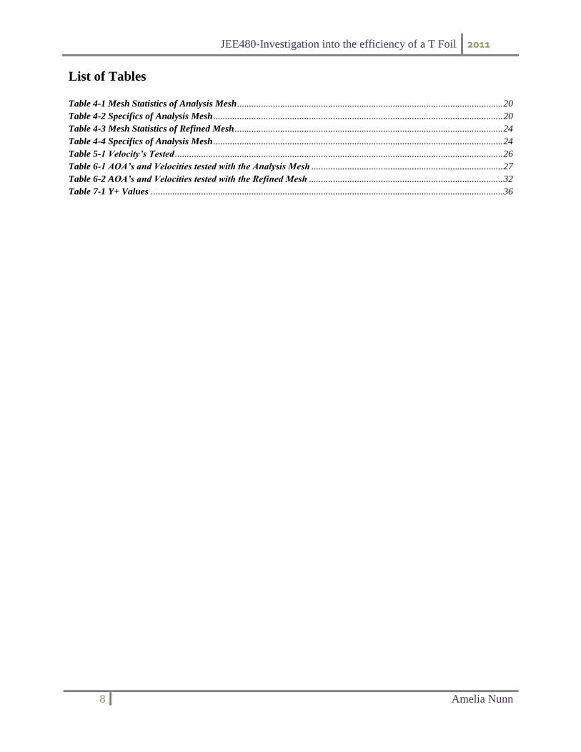
List of Tables

Table 4-1 Mesh Statistics of Analysis Mesh ............................................................................................................... 20 Table 4-2 Specifics of Analysis Mesh ......................................................................................................................... 20 Table 4-3 Mesh Statistics of Refined Mesh ................................................................................................................ 24 Table 4-4 Specifics of Analysis Mesh ......................................................................................................................... 24 Table 5-1 Velocity’s Tested ......................................................................................................................................... 26 Table 6-1 AOA’s and Velocities tested with the Analysis Mesh ................................................................................ 27 Table 6-2 AOA’s and Velocities tested with the Refined Mesh ................................................................................. 32 Table 7-1 Y+ Values ................................................................................................................................................... 36


9 Amelia Nunn

2.0 Theory

2.1 NACA Airfoils

NACA Airfoils are the resulting design of the Wright brothers’ first successful flight in the early 20th

century. Their design was developed after observing the lift developed over the curvature of a bird’s

wing. Through their initial research, the development of wings rapidly progressed resulting in the various

series’ of NACA foils.

The NACA four digit airfoil series was developed in 1933 after 78 airfoil shapes were tested in a series of

wind tunnel tests. Earlier in 1930 Eastman Jacobs of the National Advisory Committee for Aeronautics

defined the following equation for relating the airfoil thickness to the airfoil chord length;

( ) [ √

(

)

(

)

(

)

]

( )

The numbering system employed for the NACA four digit series is determined by the geometry of the foil

section. Hence, the first digit represents the maximum value of the mean line ordinate in percent of the

chord; the second digit represents the distance from the leading edge to the location of maximum camber

in tenths of the chord; and the final two digits represent the section thickness in percent of the chord

(Abbot & Doenhoff, 1959). Therefore, the NACA 00xx series represents a symmetrical section with

respect to the chord line. The cross-section of a typical NACA foil section can be seen in Figure 2-1.

Figure 2-1 NACA foil (US Department of Transportation, 1980)

The expectation of the NACA airfoil design is to deliver the maximum lift at a minimum drag. The lift

force, drag force and pitching moment are illustrated in Figure 2-2.


10 Amelia Nunn

Figure 2-2 Forces on a NACA foil (US Department of Transportation, 1980)

Approximate calculation of the forces and moments, can be found using the Equations [1], [2] and [3]

below. The approximate values of the coefficients (if unknown) are found in Figure 2-3. Incidentally,

when the forces and moments on an airfoil are determined from Tank Data or simulation programs such

as ANSYS CFX, Equations’ 1, 2 and 3 can result in determination of the moment and force coefficients.

Hence,

Lift Force,

[1]

Drag Force,

[2]

Pitching Moment,

[3]

PITCHING MOMENT


11 Amelia Nunn

Figure 2-3 Typical Wing Characteristics (Abbot & Doenhoff, 1959)

The coefficient of Lift is an important parameter as it indicates the point when the foil stops producing lift

due to boundary- layer separation. The gradual increase in flow separation can be seen in Figure 2-4.

Numerically this can be determined by plotting the Lift Coefficient against the Angle of Attack. The

Angle of Stall is found at the point went the Lift Coefficient proceeds to decrease. An example of this

phenomenon is seen in Figure 2-3.


12 Amelia Nunn

Figure 2-4 Stall - Separation of an Airfoil (NASA, 2011)

Separation characteristics are also found in the pressure distribution about the foil. The development in

pressure characteristics is seen in Figure 2-5. The pressure distribution about an airfoil is the foremost

influence on producing lift and drag on the foil. This is due to the air passing over the wing having to

travel further on the upper surface than the lower surface. Consequently lower pressures are created on

the upper surface and higher pressures generated on the lower surface which in turn generates lift.

Subsequently, as the angle of attack increases so too does the distance travelled by the airfoil which

increases the distance travelled by the foil, increasing fluid speed and thus decreasing pressure and

increasing lift. However, when the angle of attack increases to stall, the flow becomes turbulent and

initiates separation thus reducing lift but continuing the increase in drag (Swanson, -).


13 Amelia Nunn

Figure 2-5 Pressure Distribution about the foil

After the Stall Angle, vortices are found to form at the trailing edge and at the wing tip. As such, on the

trailing edges of a tapered wing, a rectangular vortex pattern occurs (this can be seen below in Figure

2-6). The rectangular pattern presented causes a constant downwash over the wing which reduces the

induced drag for a given lift and span (Moran, 1984).

Figure 2-6 Vortex pattern for a tapered wing (Graebel, 2007)

http://upload.wikimedia.org/wikipedia/commons/f/f6/Airfoils_-_pressure_diagrams.svg

http://upload.wikimedia.org/wikipedia/commons/f/f6/Airfoils_-_pressure_diagrams.svg


14 Amelia Nunn

2.2 Scaling

Reynold’s Number is employed as a scaling factor for geometrically similar shapes ie model and full

scale bodies. The non-dimensionless number can be determined from the following equation:

[ ]

Reynold’s Number was used as the velocity scaling method for the present investigation where the T Foil

was assumed to be fully submerged. The aim of this method is to conserve the viscosity rather than

produce wake – making resistance.

2.3 Turbulence model

The k-ε model is considered the industry standard when requiring both numerical and computational

accuracy. They solve the model by using the turbulent kinetic energy and its dissipation rate. Wall

functions are compulsory in this form of turbulent modelling while the y plus value must be < 300 for the

wall functions to be accurate. Limitations of the k- ε model include; separation predicted at a lower rate

and inaccuracies within the swirling flow regions.


15 Amelia Nunn

3.0 Geometry

3.1 NACA foils

The co-ordinates for the NACA foil were imported as points into Rhinoceros 4.0. The points were

obtained from the Department of Aerospace Engineering, University of Illinois (UIUC Applied

Aerodynamics Group , 2010).

According to Moran (Moran, 1984), 50 points are required for accurate airfoil geometry. Hence, to define

the NACA 0012, 132 points were imported, however, for the NACA 0015 only 32 points were imported

due to the limitations of points available. By importing such few points the accuracy of NACA 0015

geometry has been slightly affected.

After importation of the co-ordinates, the tips of the airfoil were rounded off so that fewer meshing errors

would occur (more specifically errors occurring due to sharp angles). Once the ends were rounded, Curve

Through Points was applied to create an enclosed foil. Since the t-foil involves a horizontal tapered wing,

two NACA 0012 sections were required with different chord lengths ~ 54mm and 75.6mm. Since the

NACA 0015 is in the direct centre of the tapered wing then the chord length of the strut foil was also

75.6mm. The geometry of the airfoils can be seen in Figure 3-1, Figure 3-2 and Figure 3-3.

Figure 3-1 NACA 0012a c=54mm

Figure 3-2 NACA 0012b c=75.6mm

Figure 3-3 NACA 0015


16 Amelia Nunn

3.2 Rhinoceros 4.0 Model

Rhinoceros 4.0 was used to model the T Foil from the NACA foil geometries explained previously;

Figure 3-1, Figure 3-2 and Figure 3-3

The T Foil specified was physically measured to enable accurate modelling. To capture the extent of the

flow characteristics the T Foil was initially scaled to 9% in Rhinoceros 4.0, however, it was later scaled

up to 54% (in ANSYS 12.1 Geometry) of the measured T Foil to improve the results produced in ANSYS

CFX Post. The dimensions of the T Foil can be seen in Figure 3-4 and Figure 3-5.

Figure 3-4 Perspective view of T Foil

Figure 3-5 Top View of T Foil

The horizontal foil and strut were individually modelled in Rhinoceros 4.0 for ease of importation into

ANSYS 12.1 Geometry. The horizontal foil was modelled using the two NACA 0012 foils (NACA 0012a

and NACA 0012b). After being imported onto the same plane, two lines connecting the trailing edges and

leading edges were drawn; enabling the Sweep 2 function to be employed to create one surface. The

surface was subsequently mirrored and Capped to close off the ends of the foil. The horizontal foil was


17 Amelia Nunn

then Split as seen in Figure 3-6. The Boolean Union function was subsequently used to join the horizontal

foil into a singular Polysurface.

The vertical strut with the NACA 0015 was next modelled in Rhinoceros 4.0. The image seen in Figure

3-3 was extruded perpendicular to the plane of horizontal foil. After extrusion, the foil was Capped to

close off the open ends of the strut and subsequently Split (this is seen in Figure 3-7). After the successful

split the strut was joined using the Boolean Union Function.

Splitting the foil is an important modelling aspect as it facilitates the option of refining the mesh at the

leading and trailing edges which enables accurately capturing the flow characteristics.

Figure 3-6 Splits in Horizontal Foil

Figure 3-7 Splits in Strut


18 Amelia Nunn

3.3 Domain

The domain for the fluid flow analysis, found below in Figure 3-8, was constructed in ANSYS 12.1

Geometry. Due to mesh size limitations, Figure 3-8, is a symmetrical half section of the domain. Since

both the domain and T Foil are symmetrical, then splitting directly through the middle is possible.

The shape of the domain originated as a rectangle but as the front top and bottom edges of the rectangle

inlet do not assist with the flow characteristics then these were removed and replaced by a semi-circular

shape to save on mesh elements. The rectangle found at the back of the domain was implemented so that

the mesh size in this region could be increased to reduce the mesh size (although this feature of the

geometry was never implemented in meshing). Another feature of the domain is the inner cylinder which

contains the foil (seen in Figure 4-2) which assists in creating a fine mesh around the T Foil and flow

regions about the T Foil.

The domain size was determined upon using 11 x the maximum chord length (NACA 0015) for the flow

region behind the foil and 5 x the maximum chord length (NACA 0015) for the flow region; above, below

and in front of the foil.

Figure 3-8 Domain


19 Amelia Nunn

4.0 Mesh

The meshing method employed was CFX mesh in ANSYS 12.1 Meshing Application. A maximum

specification of 500,000 elements was required in completing the analysis of the T Foil. To precisely

determine mesh size, a Grid Independence Study was executed. With reference to Figure 4-1, the mesh

size required to produce an accurate results is at ~460,000 elements.

4.1 Grid Independence Study

Figure 4-1 Grid Independence Study

4.2 Analysis Mesh

The Analysis Mesh sizing was produced as a result of the grid independence study. Table 4-1 displays the

mesh size for an Angle of Attack of 16 degrees as this was the maximum mesh size implemented. An

overview of the sizing of the mesh is seen in Table 4-2.

2.4

2.45

2.5

2.55

2.6

2.65

2.7

2.75

- 200,000 400,000 600,000 800,000 1,000,000 1,200,000 1,400,000

Lif

t F

orc

e (

N)

Number of Mesh Elements

Initial Point of Convergence


20 Amelia Nunn

Table 4-1 Mesh Statistics of Analysis Mesh

Table 4-2 Specifics of Analysis Mesh

Default Body Spacing

Maximum size 30 mm

Default Face Spacing

Minimum Edge Length 3 mm

Maximum Edge Length 30 mm

Inflated boundary

Maximum Thickness 1.2 mm

Edge spacing (At trailing edge)

Minimum Edge Length 1.5 mm

Maximum Edge Length 6 Mm

Default Face Spacing and Default Body Spacing were used in defining the mesh in the main body

domains. The mesh in the cylindrical section was refined to concentrate the flow in this region. It can be

seen in Figure 4-2 that the mesh starts off coarse and is refined as it approaches the T Foil.

Figure 4-2 Domain mesh at AOA 12 degrees


21 Amelia Nunn

Figure 4-3 displays the concentrated mesh about the leading and trailing edges. The mesh has been

concentrated in these areas so that the vortices and areas of separation can be accurately captured.

Figure 4-3 Analysis Mesh about the T-Foil


22 Amelia Nunn

As previously explained the T Foil was split into sections to increase the mesh spacing in the areas of

interest. A detailed view of the splits with varying mesh spacing is seen in Figure 4-4. Face Spacing was

used over the split faces, while Edge Spacing was used at the trailing edge of the horizontal foil.

Figure 4-4 Splits through T-Foil

Edge Spacing


23 Amelia Nunn

An Inflated Boundary was applied to the entirety of the T Foil to remove sharp mesh angles. Referring to

Figure 4-5, the inflated boundary has ensured a satisfactory transition mesh for merging the T Foil to the

cylinder.

Figure 4-5 Inflated Boundary

Inflated

Boundary


24 Amelia Nunn

4.3 Refined Mesh

The Refined Mesh seen in Figure 4-6 and Figure 4-7 was developed by reducing the sizing of the

analysis mesh by approximately 30%. The mesh size for the refined mesh is displayed in Table 4-3 for

an Angle of Attack of 0 degrees. An overview of the sizing of the mesh is seen in Table 4-4.

Table 4-3 Mesh Statistics of Refined Mesh

Table 4-4 Specifics of Analysis Mesh

Default Body Spacing

Maximum size 30 mm

Default Face Spacing


Maximum Edge Length 30 mm

Inflated boundary

Maximum Thickness 0.36 mm

Edge spacing (At trailing edge)


Maximum Edge Length 1.8 mm


25 Amelia Nunn

Figure 4-6 Refined Mesh – Domain

Figure 4-7 Refined Mesh


26 Amelia Nunn

5.0 Setup

The Domain Setup is constant for all mesh variations as it is seen in Figure 5-1. The Boundary Conditions

set are as follows; Inlet was set as ‘Inlet’, Outlet was set as ‘Opening’, Sym-Side was set as ‘Symmetry’,

T Foil was set as a ‘No-Slip Wall’, and the Top, Side Wall and Base were set as a ‘Free-Slip Wall’. The

turbulence model applied was K - Epsilon.

Figure 5-1 Domain Setup

The model velocities applied to all runs are found in Table 5-1. The model velocities were scaled using

Reynolds scaling found previously in Equation [4];

Table 5-1 Velocity’s Tested

La (mm) 140 140 140 140

Lm (mm) 75.66 75.66 75.66 75.66

Va (m/s) 0.5 1.125 1.75 2.4

Vm (m/s) 0.9 2.1 3.2 4.4

Inlet

Outlet

Sym-Side

Side Wall Top

Base T-Foil


27 Amelia Nunn

6.0 Results

6.1 Analysis Mesh

The Analysis Mesh tested a wide range of Angles of Attack which can be found in Table 6-1. The

extensive range of AOA’s tested was applied to accurately depict the exact point at which the Stall

Angle would occur. Hence at 0.9 m/s, Stall occurred at an AOA of 13 degrees while at the higher

velocities (2.1m/s, 3.2m/s and 4.4m/s), Stall occurred at an AOA of 12.5 degrees. Although a

maximum AOA of 15 degrees was specified, 2008 Tank Data (Jonathan R. Binns, 2008) revealed

that Stall occurred at 15 degrees, hence to isolate when the Stall Angle occurred it was necessary to

examine the angle after stall hence 16 degrees was tested.

Table 6-1 AOA’s and Velocities tested with the Analysis Mesh

AOA ( ° ) V [m/s]

0 0.9 2.1 3.2 4.4

3 0.9 2.1 3.2 4.4

6 0.9 2.1 3.2 4.4

7 0.9 2.1 3.2 4.4

8 0.9 2.1 3.2 4.4

9 0.9 2.1 3.2 4.4

10 0.9 2.1 3.2 4.4

11 0.9 2.1 3.2 4.4

12 0.9 2.1 3.2 4.4

12.5 - 2.1 3.2 4.4

13 0.9 2.1 3.2 4.4

14 0.9 2.1 3.2 4.4

15 0.9 2.1 3.2 4.4

16 0.9 2.1 3.2 4.4


28 Amelia Nunn

6.1.1 CFD Data

The following Figures; Figure 6-1, Figure 6-2 and Figure 6-3 present the data obtained directly

from ANSYS 12.1 CFX Post.

Figure 6-1 Analysis Mesh – L vs AOA

Figure 6-2 Analysis Mesh – D vs AOA

Figure 6-3 Analysis Mesh – M vs AOA

0

10

20

30

40

50

60

70

80

0 2 4 6 8 10 12 14 16 18

Lif

t F

orc

e (

N)

Angle of Attack, α

0.9

2.1

3.2

4.4

0

5

10

15

20

25

0 2 4 6 8 10 12 14 16 18

Dra

g F

orc

e (

N)

Angle of Attack, α

0.9

2.1

3.2

4.4

-3.5

-3

-2.5

-2

-1.5

-1

-0.5

0

0.5

0 2 4 6 8 10 12 14 16 18

Pit

chin

g M

om

en

t (J

)

Angle of Attack, α

0.9

2.1

3.2

4.4


29 Amelia Nunn

6.1.2 CFD Data Calculations

The following Figures; Figure 6-4, Figure 6-5 and Figure 6-6 are the product of using the CFD

Post results with Equations [1], [2] and [3].

Figure 6-4 Analysis Mesh - CL vs AOA

Figure 6-5 Analysis Mesh – CD vs AOA

0

0.1

0.2

0.3

0.4

0.5

0.6

0.7

0.8

0 2 4 6 8 10 12 14 16 18

Lif

t C

oe

ffic

ien

t

Angle of Attack, α

0.9

2.1

3.2

4.4

0

0.05

0.1

0.15

0.2

0.25

0 2 4 6 8 10 12 14 16 18

Dra

g C

oe

ffic

ien

t

Angle of Attack, α

0.9

2.1

3.2

4.4


30 Amelia Nunn

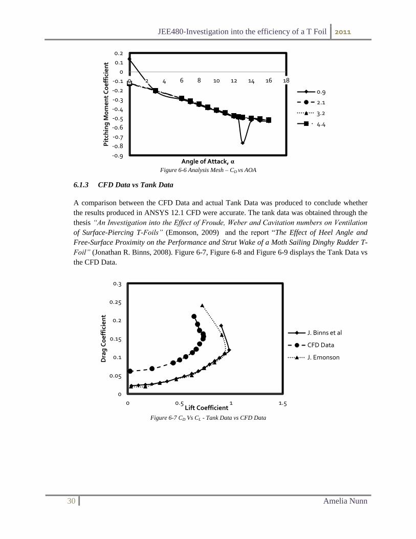
Figure 6-6 Analysis Mesh – CD vs AOA

6.1.3 CFD Data vs Tank Data

A comparison between the CFD Data and actual Tank Data was produced to conclude whether

the results produced in ANSYS 12.1 CFD were accurate. The tank data was obtained through the

thesis “An Investigation into the Effect of Froude, Weber and Cavitation numbers on Ventilation

of Surface-Piercing T-Foils” (Emonson, 2009) and the report “The Effect of Heel Angle and

Free-Surface Proximity on the Performance and Strut Wake of a Moth Sailing Dinghy Rudder T-

Foil” (Jonathan R. Binns, 2008). Figure 6-7, Figure 6-8 and Figure 6-9 displays the Tank Data vs

the CFD Data.

Figure 6-7 CD Vs CL - Tank Data vs CFD Data

-0.9

-0.8

-0.7

-0.6

-0.5

-0.4

-0.3

-0.2

-0.1

0

0.1

0.2

0 2 4 6 8 10 12 14 16 18

Pit

chin

g M

om

en

t C

oe

ffic

ien

t

Angle of Attack, α

0.9

2.1

3.2

4.4

0

0.05

0.1

0.15

0.2

0.25

0.3

0 0.5 1 1.5

Dra

g C

oe

ffic

ien

t

Lift Coefficient

J. Binns et al

CFD Data

J. Emonson


31 Amelia Nunn

Figure 6-8 CD vs AOA - Tank Data vs CFD Data

Figure 6-9 CL vs AOA - Tank Data vs CFD Data

0

0.05

0.1

0.15

0.2

0.25

0.3

0 2 4 6 8 10 12 14 16 18

Dra

g C

oe

ffic

ien

t

Angle of Attack, α

J. Binns et al

CFD Data

J. Emonson

0

0.2

0.4

0.6

0.8

1

1.2

0 2 4 6 8 10 12 14 16 18

Lif

t C

oe

ffic

ien

t

Angle of Attack, α

J. Binns et al

CFD Data

J. Emonson


32 Amelia Nunn

6.2 Refined Mesh

The Refined Mesh was tested at an Angle of Attack of 0 degrees at four different speeds (Tested

speeds can be seen in Table 6-2. The four speeds were tested to enable a distinct comparison

between the two mesh sizes.

Table 6-2 AOA’s and Velocities tested with the Refined Mesh

AOA ( ° ) V [m/s]

0 0.9 2.1 3.2 4.4

6.2.1 Refined Mesh vs Analysis Mesh

Figure 6-10 Refined Mesh vs Analysis Mesh

-2

-1

0

1

2

3

4

5

6

7

0 1 2 3 4 5

Force [N] Pitching Moment[J] Velocity [m/s]

Drag - Refined Mesh

Drag - Analysis Mesh

Lift - Refined Mesh

Lift - Analysis Mesh

Moment - Refined Mesh

Moment - Analysis Mesh


33 Amelia Nunn

7.0 Discussion

7.1 Grid Independence Study

The Grid Independence Study (Figure 4-1) revealed the instance at which the mesh was refined

enough to produce adequate results. The number of elements required to produce good results was in

range of the 500,000 elements specified – the maximum being ~490,000 elements @ AOA of 16

degrees.

7.2 Convergence

Convergence was seen in the solutions of a majority of the runs. Though, at an AOA of 16 degrees

with velocities; 2.1 m/s, 3.2 m/s and 4.4 m/s the results failed to converge. However, since all the

runs prior to these converged it was disregarded and assumed to be due to possible meshing issues.


34 Amelia Nunn

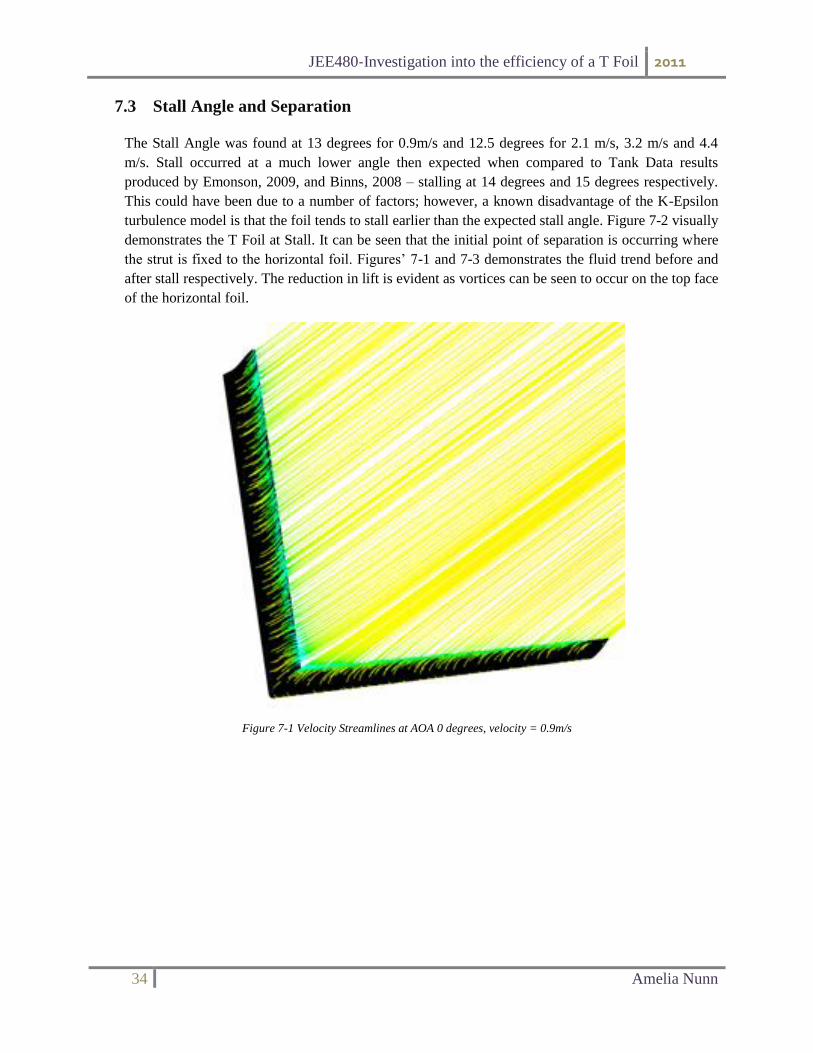
7.3 Stall Angle and Separation

The Stall Angle was found at 13 degrees for 0.9m/s and 12.5 degrees for 2.1 m/s, 3.2 m/s and 4.4

m/s. Stall occurred at a much lower angle then expected when compared to Tank Data results

produced by Emonson, 2009, and Binns, 2008 – stalling at 14 degrees and 15 degrees respectively.

This could have been due to a number of factors; however, a known disadvantage of the K-Epsilon

turbulence model is that the foil tends to stall earlier than the expected stall angle. Figure 7-2 visually

demonstrates the T Foil at Stall. It can be seen that the initial point of separation is occurring where

the strut is fixed to the horizontal foil. Figures’ 7-1 and 7-3 demonstrates the fluid trend before and

after stall respectively. The reduction in lift is evident as vortices can be seen to occur on the top face

of the horizontal foil.

Figure 7-1 Velocity Streamlines at AOA 0 degrees, velocity = 0.9m/s


35 Amelia Nunn

Figure 7-2 Velocity Streamlines at Stall (13 degrees), velocity 0.9 m/s

Figure 7-3 Velocity Streamlines after Stall (16 degrees), v= 0.9 m/s


36 Amelia Nunn

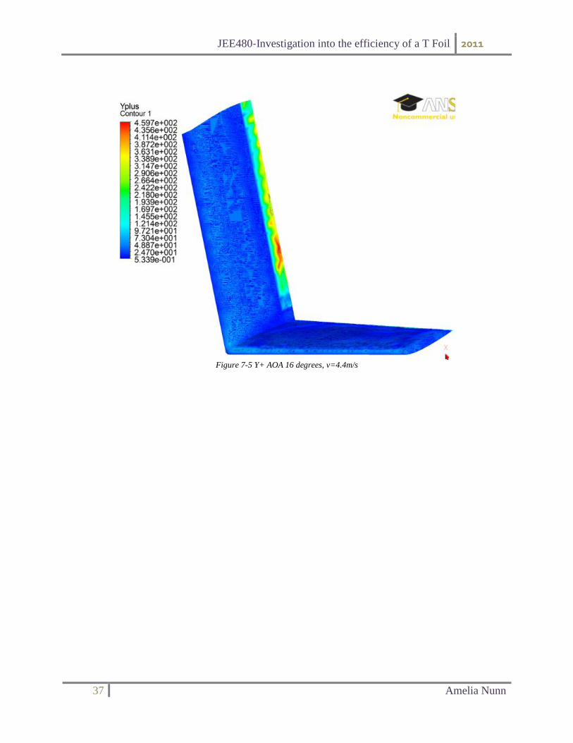
7.4 Y+

The Y+ values revealed in Table 7-1 capture the range of Y+ values found over a variety of the

Angles of Attack. When using k-epsilon turbulence models the maximum Y+ value should be no

greater than 300, however, it is revealed that at an AOA of 16 degrees at v = 4.4 m/s the Y+ value

equals 460. Hence, for the final angle and final velocity tested it is outside the range of acceptable

Y+ values. Figure 7-4 and display the T Foils which resulted in the minimum and maximum Y+

values found in the results (Table 7-1). Figure 7-5 displays that the highest y plus values occur on the

strut while Figure 7-4 shows very low Y+ values on the strut (the maximum occurring on the trailing

edge of the horizontal foil). The high Y+ value could be reduced if the mesh size along the trailing

edge of the strut was reduced.

Table 7-1 Y+ Values

Y +

AOA 0, v=0.9 55

AOA 0, v=4.4 240

AOA 12.5, v=4.4 269

AOA 13, v=0.9 60

AOA 16, v=0.9 108

AOA 16, v=4.4 460

Figure 7-4 Y+ AOA 0 degrees, v=0.9m/s


37 Amelia Nunn

Figure 7-5 Y+ AOA 16 degrees, v=4.4m/s


38 Amelia Nunn

7.5 Pressure Development

The pressure images produced (Figure 7-6, Figure 7-7, Figure 7-8) are in direct correlation with the

theoretical expectations found in Figure 2-5. It can be seen that there is an even pressure acting about

the foil at 0 AOA; at 13 AOA the maximum pressure is seen at the lower stagnation point before

traversing to the top as seen in Figure 7-8.

Figure 7-6 Pressure @ AOA 0 degrees, v=0.9m/s



39 Amelia Nunn



40 Amelia Nunn

7.6 Vortices Progress

Figures’ 7-9, 7-10 and 7-11, clearly identify the increase in vortices as the Angles of Attack increase.

It can be seen that even at 0 AOA the vortices have already began to form at the tip and over the foil.

As the foil reaches stall, the vortices begin to form at the trailing edge while the vortices at the tip are

further increased than that of 0 AOA. At 16 AOA the pressure distribution has translated to the top of

the foil which has induced large vortices acting midway over the foil – the point at which separation is

at its maximum.

Figure 7-9 Vortices @ AOA 0 degrees, v=0.9m/s


41 Amelia Nunn




42 Amelia Nunn

7.7 Lift, Drag and Pitching Moment

The Lift Force, Drag Force and Pitching Moment results found in Figure 6-1, Figure 6-2 and Figure

6-3 reveal that at the Angle of Stall - the Lift, Drag and Pitching Moment are at their maximum. At

higher velocities the gradient of the forces and moments increases more rapidly than when at lower

speeds. With reference to Figure 7-12 below, the Lift/Drag Ratio is at its maximum when the Angle of

Attack is at ~9 degrees, hence this reveals that the foil will be of the highest efficiency at an AOA of 9

degrees.

Figure 7-12 Analysis Mesh – Lift/Drag vs Angle of Attack

The Coefficients were calculated using the force and moment data provided from ANSYS 12.1 CFX

Post. Figure 6-4 and Figure 6-5 reveal the Lift and Drag coefficients respectively. An obvious trend is

seen through the results providing evidence that the fluid simulation program was accurate. However,

observing the trends in the pitching moment coefficients seen in Figure 6-6; there is a definitive jump

at 13 AOA when the velocity is 0.9m/s. As mentioned before the T Foil stalls at 13 AOA when the

velocity is at 0.9m/s, hence the jump in Pitching Moment coefficient data could be due to the change

in pressures on the foil.

7.8 Analysis Mesh CFD Data vs. Tank Data

The comparison between the CFD Data and Tank Data (Figure 6-7, Figure 6-8 and Figure 6-9) reveals

a discrepancy between results but a comparable trend in data. The discrepancy is partly due to

different speeds tested. The CFD Data applied in the comparison was at a scaled speed of 4.4 m/s

while the equivalent speed for the tested data is 7.7 m/s. While this inconsistency hinders whether the

results can be accurately compared, the trend between the data indicates that the CFD data is accurate.

7.9 Analysis Mesh vs. Refined Mesh The Refined Mesh was without element size restriction however the analysis continued to focus on

half of the domain. The mesh size was increased by about 1.5 million elements which highly increased

the accuracy of the results. A comparison between the analysis mesh and refined mesh is found in

Figure 6-10. A noticeable difference in drag force, lift force and pitching moment was found that there

was a greater lift, smaller drag and lesser pitching moment with respect to the analysis mesh.

0

1

2

3

4

5

6

7

0 2 4 6 8 10 12 14 16 18

Lif

t / D

rag

Angle of Attack, α

0.9

2.1

3.2

4.4


43 Amelia Nunn

8.0 Conclusion

The CFD results were found to be in good agreement with the 2008 and 2009 experimental data

[ (Jonathan R. Binns, 2008) and (Emonson, 2009) ].

The Stall Angle was found to be at 13 degrees at a velocity of 0.9 m/s and 12.5 degrees at a velocity of

2.1, 3.2 and 4.4 m/s. Both stall angles were below the tank data results [ (Emonson, 2009)& (Jonathan R.

Binns, 2008)], however, this could be due to inaccuracies found with the k-epsilon model or

inconsistencies found within the mesh. A review of the Y+ values reveals that at the maximum; angle and

velocity, the Y+ value was outside the range deemed acceptable for the k-epsilon model i.e. > 300. The

Y+ value was found to be at its greatest at the trailing edge of the strut hence if the mesh size was reduced

on this edge, the Y+ value could be within the acceptable range and the T Foil might have stalled at the

expected angle.

The refined mesh enhanced the results produced to that of the analysis mesh, however, the results could

further be improved if the model wasn’t scaled to 54% and the entire foil and domain were analysed.

The development of the pressure distribution was in line with the theoretical expectation of Figure 2-5.

With reference to Figures’ 7-1, 7-2 and 7-3 the development of separation is clearly exhibited. The effect

of the separation can also be observed in the vortex regions in Figures’ 7-9, 7-10 and 7-11.

The T Foil was found to be the most efficient when at an Angle of Attack of 9 degrees due to the

Lift/Drag ratio being at its maximum. For the best performance in Lift the T Foil should be operated at 9

degrees.


44 Amelia Nunn

9.0 Recommendations

The major inconsistency found in the results was concluded to be due to mesh size and k-epsilon

turbulence modelling.

The author recommends the following:

Develop a finer mesh at the trailing edge of the strut to reduce Y+ values and increase the stall

angle

Investigate the results produced by other Turbulence Models such as the Shear Stress Turbulence

modelling

Scale the T Foil closer to the actual size or do not scale at all

Explore the possibility of applying winglets to the tip of the horizontal foil to reduce the vortices


45 Amelia Nunn

10.0 References

Abbot, I., & Doenhoff, A. (1959). Theory of Wing Sections. Toronto: General Publishing Company.

Emonson, J. (2009). An Investigation into the Effect of Froude, Weber and Cavitation numbers on

Ventilation of Surface-piercing T-Foils. Launceston: AMC.

Graebel, W. (2007). Advanced Fluid Mechanics. London: Elsevier.

Jonathan R. Binns, P. A. (2008). The Effect of Heel Angle and Free-Surface Proximity on the

Performance and Strut Wake of a Moth Sailing Dinghy Rudder T-Foil . Auckland: 3rd High

Performance Yacht Design Conference .

Moran, J. (1984). An Introduction to Theoretical And Computational Aerodynamics. New York: John

Wiley & Sons.

NASA. (2011, 04 08). Introduction to the Aerodynamics of Flight. Retrieved 04 26, 2011, from NASA

History: http://history.nasa.gov/SP-367/f48.htm

NSIT. (2009). About IGES. Retrieved 03 26, 2011, from Technology Services:

http://ts.nist.gov/standards/iges/about.cfm

Swnason, D. Dr. (-). INTRODUCTION / ADAPTATIONS FOR FLIGHT . Retrieved 04 26, 2011, from

Biology 463/563 Ornithology: http://people.usd.edu/~dlswanso/ornith/lec1_2.html

UIUC Applied Aerodynamics Group . (2010). UIUC Airfoil Coordinates Database. Retrieved 04 25,

2011, from UIUC Applied Aerodynamics Group : http://www.ae.illinois.edu/m-selig/

US Department of Transportation. (1980). Flight Training Handbook. Retrieved 04 24, 2011, from

Aviation Online Magazine: http://avstop.com/ac/flighttrainghandbook

investigation into the efficiency of a t foil

Documents