investigation and implementation of non- …511820/fulltext01.pdf · investigation and...

INVESTIGATION AND IMPLEMENTATION OF NON-

LINEAR MICRO PLASTICITY IN ABAQUS

AUTHOR: MOHAMMAD TAVAKOL

DIPLOMA WORK FOR MASTER SCIENCE (MSC.), KTH

WORK CARRIED OUT AT SWEREA KIMAB, STOCKHOLM KTH PRODUCTION ENGINEERING

KUNGLIGA TEKNISKA HÖGSKOLAN, HT-11

EXAMENSARBETE 2011-12-31

STOCKHOLM

Abstract

This thesis is aimed to investigate different approaches in FEM simulation of sheet metal

forming to accurately predict the final geometry. These approaches are mainly focused

on the behavior of material models used in the forming process. Two sets of test results

are available that play important roles in this project. The first set is the cyclic test which

depicts the behavior of the material model in large deformations. The material model in

simulations is modified according to the cyclic test results. Second set of tests is Bending

Under Tension (BUT) test which represents the forming process of sheets. BUT test is

simulated with the material model that is modified according to the cyclic test results.

The deformed profiles of the BUT simulations are compared with BUT test results to

check the accuracy of the modified material models.

The influence of friction on the final geometry in the BUT simulations is investigated. All

of the modified material models are implemented in simulations with and without considering friction and the results are compared. Friction provides a realistic condition

in BUT simulation and has a great impact in spring-back results. Friction reduces the

bending stiffness of sheets and consequently the more spring-back is observed. The

modified model with single step reduction in elastic modulus (with friction) makes an

improvement in prediction of spring-back magnitude in BUT simulation.

3

Acknowledgment

I would like to express my sincere gratitude to my supervisor Niclas Stenberg for his

immense practical help in initiation, evolution and completion of this thesis work. His

erudite supervision and kind encouragement made a great contribution in fulfilling the

goals of this project. I am deeply indebted to Arne Melander for his patient support and

valuable hints during all steps of this work. I would like to thank my colleagues in KIMAB

for providing me with kind supports and friendly environment during my thesis.

Furthermore, I wish to thank my parents for their unbroken and progressive support

which has played a significant role in all my achievements particularly my educational

improvements. Finally I would like to thank Soolmaz, for her love and patience.

Table of content Abstract ...................................................................................................................................... 2

Acknowledgment .................................................................................................................... 3

Table of content .......................................................................................................................... 4

1 Introduction ........................................................................................................................ 6 1.1 Objective ..................................................................................................................... 6

1.2 History ......................................................................................................................... 6

1.2.1 Higher order terms in elastic theory ..................................................................... 6

1.2.2 Micro-plastic mechanism and the Bauschinger effect ........................................... 7

1.2.3 Hardening behavior of metals .............................................................................. 8

2 Material and methods ......................................................................................................... 9

2.1 Material properties ...................................................................................................... 9

2.2 Materials model ........................................................................................................... 9

2.2.1 Kinematic hardening model .................................................................................. 9

� Linear kinematic hardening model ............................................................................. 10 � Isotropic/kinematic hardening model ........................................................................ 10

2.2.2 Nonlinear Isotropic/ Kinematic hardening Chaboche - Lemaitre model............... 11

2.3 Modifications of the Elastic modulus according to cyclic tests .................................... 11

2.3.1 Cyclic tests ......................................................................................................... 12

� Experimental results from the cyclic tests .................................................................. 12

2.3.2 Method for extracting the tangent modulus from the tests ................................ 15

2.3.3 Short Discussion of instant Young’s modulus results ........................................... 16

2.4 Implementing the modified material modulus in ABAQUS by aid of USDFLD .............. 16

2.4.1 Introduction to FEM ........................................................................................... 16 2.4.2 USDFLD (user subroutine defined field variables) ............................................... 17

2.5 Basic model for implementing modified material model in FE analysis ....................... 17

� Geometry & Boundary condition ............................................................................... 18

� Loading ...................................................................................................................... 18

2.6 Verification of the modified material modulus ........................................................... 18

2.6.1 BUT test ............................................................................................................. 18

2.6.2 BUT test machine ............................................................................................ 19

2.6.3 BUT simulation ................................................................................................... 20

� Geometry & Boundary condition ............................................................................ 20

� Elements and mesh .................................................................................................... 21 3 Results............................................................................................................................... 22

3.1 Basic model ............................................................................................................... 22

3.1.1 Unacceptable Modification of elastic modulus ................................................... 22

� Modification of elastic modulus as a function of back-stress ...................................... 22

� Smoothening the undesired jumps in tangent modulus ............................................. 23

5

3.1.2 Acceptable Modifications of elastic modulus ...................................................... 24

� Single reduction of elastic modulus ............................................................................ 24

� Modification of elastic modulus by stress invariant .................................................... 25

3.2 BUT Simulation results ............................................................................................... 26

3.2.1 BUT simulation input .......................................................................................... 26 � Modified material models........................................................................................ 26

� Brake force .............................................................................................................. 27

� Coefficient of friction ............................................................................................... 27

3.2.2 Profile & radius of spring-back ............................................................................ 27

3.2.3 The impact of friction on the spring-back profile ................................................ 37

4 Discussion ......................................................................................................................... 38

4.1 Overview ................................................................................................................... 38

4.2 Conclusion ................................................................................................................. 39

4.2.1 Impact of friction................................................................................................ 39

4.2.2 First modification (single reduction of elastic modulus) ...................................... 39 4.2.3 Second modification (modification of elastic modulus by stress invariants) ........ 39

4.3 Future work ............................................................................................................... 39

5 References ........................................................................................................................ 40

6 Appendix ........................................................................................................................... 42

� Apendix1 ....................................................................................................................... 42

FORTRAN codes for modification of material model .............................................................. 42

- FORTRAN code for single reduction in elastic modulus ............................................... 42

- FORTRAN code for cyclic variation of elastic modulus as a function of back stress ...... 42

- FORTRAN code for cyclic modification with back stress (Smoothening with ArCTAN

function)............................................................................................................................ 43 - FORTRAN code for cyclic modification as a function of stress invariants ..................... 44

� APENDIX2 ...................................................................................................................... 47

Octave code for extracting results from tests and simulation ................................................ 47

- Octave code for extracting elastic modulus from cyclic tests ...................................... 47

- Octave code for extraction of the instant elastic from the simulation ......................... 48

1 Introduction

Sheet metal stamping introduces a complex plastic deformation in the sheets. When the punch

and die are removed after a forming step, recovered portion of deformation results in a change

in the final shape of the part. This is a subject of major concern in design of the tools for sheet

metal panels. Inaccurate prediction of spring-back may result in tool geometries that produce

inaccurate deformation in the parts. Therefore a precise description of recoverable strain during

unloading is needed.

1.1 Objective

The aim of this thesis is to perform simulations where spring-back is in focus and verify them

with experimental results. Since test results have reported a change in elastic modulus with

plastic deformation, it is desired to control the elastic modulus by aid of field variables (USDFLD)

in ABAQUS. The magnitude of spring-back deformation is related to several factors. One of these

factors is the level of plastic strain. Stress invariants are another factor that affects spring-back

deformation. The modified modulus will be utilized in BUT test simulations. The results of BUT

simulation are verified with the BUT test results. In BUT simulations friction is another factor that affects the magnitude of spring-back. Therefore

simulations have been performed with friction and frictionless and the results are analyzed.

1.2 History Predicting the spring-back magnitude of sheets after punching has been in focus for a long time.

The problem emerged while different spring-back behavior was observed in punching process.

Initially practical methods were used to investigate the important factors in this phenomenon.

Back to 1964, Baba and Tozawa [1] focused on the effect of stretching a sheet by a tensile force,

during or after bending, in minimizing spring-back deviation.

Afterward effort was mainly focused on the possible reasons of this phenomenon. There are

many hypothesis proposed for this phenomenon that are categorized in three main areas:

- The impact of higher order terms in theory of elasticity.

- The impact of Micro-plastic mechanism and the Bauschinger effect on spring-back.

- The impact of Hardening behavior of metals on magnitude of spring-back.

1.2.1 Higher order terms in elastic theory

7

Higher order terms in elastic theory has been a subject of interest for justifying the spring-back

in metals. To obtain a better appreciation for this nonlinear behavior, it is worth remembering

that elastic behavior is the result of atomic bond stretching. It is generally assumed to be linear

because this is a good first order approximation. However, rigorous application of elastic theory

includes higher order terms that lead to a small amount of nonlinear recovery. Wong and Johnson [2] investigated the amount of nonlinearity in loading and unloading attributable to

higher order elastic constants for some common alloys. A departure from linearity has been

noted, but it is rather small. Typically the expected total spring-back exceeds the linear spring-

back by less than 3% but the change in average effective modulus found by Cleveland and Ghosh

[3] is about 22% for high strength steel.

1.2.2 Micro-plastic mechanism and the Bauschinger effect

Investigations and Experimental tests have proved that the elastic modulus of metals in loading

and unloading is not the same and this difference will influence the magnitude of spring-back

[3]. One of the possible reasons for this variation is Bauschinger effect which is known as early

yielding under reversed loading. Stout and Rollett [4] declared that The Bauschinger effect is

explained in terms of the easy motion of piled up dislocations and unraveling of dislocation

structures when the loading direction is reversed. Cleveland and Ghosh ascribe the apparent

reduction of the elastic modulus to presence of mobile dislocations which can move due to the

internal repulsive forces between them once the external force on the material are removed.

They tried to confirm that the recovery is micro-plastic in nature by waiting several days after the pre-strain is exposed. They observed that the extent of the nonlinear effect is minimized

which could be considered as a clear sign of dislocation annihilation effect [3].

In order to have a better understanding of Bauschinger effect on spring-back phenomenon, it

should be considered that sheet punching is a procedure which often includes one bending and

one unbending (tensile loading, unloading, compression). The reduction of elastic modulus in

reverse loading in punching results in variation of elastic modulus in a loading cycle.

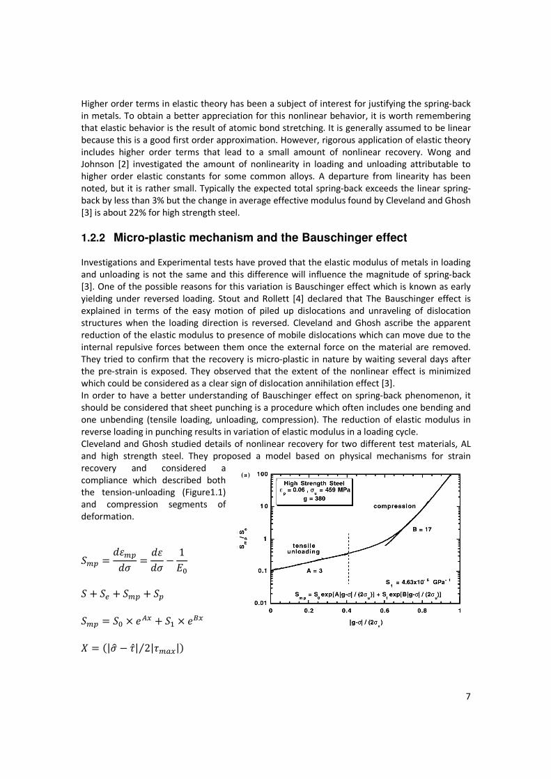
Cleveland and Ghosh studied details of nonlinear recovery for two different test materials, AL

and high strength steel. They proposed a model based on physical mechanisms for strain

recovery and considered a

compliance which described both the tension-unloading (Figure1.1)

and compression segments of

deformation.

�� 1�

� � � � ��

��

� � �|�� ̂| 2|��|⁄ �

• is the linear elastic compliance

• is the large scale plastic compliance that will eventually dominate as yielding occurs.

• A and B are known linear functions of equivalent plastic pre-strain

• is floating ‘‘effective’’ stress, including its sign, is defined by

• is a multi-axial measure of internal stress, analogous to the g.

• is the floating value of when the principal stress rate last changed its sign.

This suggests that there is a nearly universal equation for strain recovery during unloading and

reverse loading with slight changes in the constants and . They observed that the reverse

plastic yielding is clearly gradual. Therefore it is more meaningful to describe yield by a stress at

which becomes about 5–10% of the initial modulus (i.e. 0.05 to 0.1 ). This is

believed to be the onset of macro-plasticity as suggested by a more rapid decay in the

instantaneous tangent modulus.

1.2.3 Hardening behavior of metals Hardening behavior of metals is another important factor which affects the spring-back. The

Chaboche - Lemaitre - Lemaitre model has gained some popularity in recent years. In this model

a recall term is introduced to realize the smooth elastic-plastic transition behavior [6, 7]. The

combined isotropic-kinematic hardening law is considered suitable in predicting the spring-back. S. L. Zang et al. [5] simulated spring-back with an elastic-plastic constitutive model based on

isotropic non linear kinematic (INLK) hardening model of Chaboche - Lemaitre type rule and

Hill’s 1948 anisotropic yield function. In this model the elastic modulus changes with plastic

strain. The simulation results, especially the sheet spring-back obtained with the isotropic non

linear kinematic hardening, in which the change of Young’s modulus with plastic deformation is

considered, agree well with experiments. The study indicates that the isotropic hardening (IH)

law overestimates the Bauschinger effect. When the non-linear kinematic (NLK) hardening is

used, the spring-back amount is considerably underestimated, suggesting that Chaboche -

Lemaitre kinematic hardening model is not adequate to predict the spring-back.

Numerical and experimental results shows that in modeling Bauschinger effect, the change of Young’s modulus with plastic deformation appears to be more important when multiple cycles

of loading _ unloading is considered, Therefore Chaboche - Lemaitre - Lemaitre mixed hardening

model is not accurate in multi cycle simulations.[3]

R. Cobo et al.[8] performed experimental test (die punch) to determine the apparent young

modulus and introduced an unloading constant modulus in unloading from the experimental

results. They simulated their test with different modulus in loading and unloading. In the

beginning of unloading they switched the elastic modulus to unloading modulus by aid of

USDFLD in ABAQUS. They have calculated by assuming an elastic unloading from the

experimental results. By this method their deviation from the experimental result was much

smaller than using a constant Elastic modulus in loading and unloading. Vin et al. [9] gave a simple mathematical model describing the relationships between plastic deformation and

Young’s modulus based on experiment results.

τ

Figure1.1 Compliance diagram for nonlinear unloading in

high strength steel

9

2 Material and methods

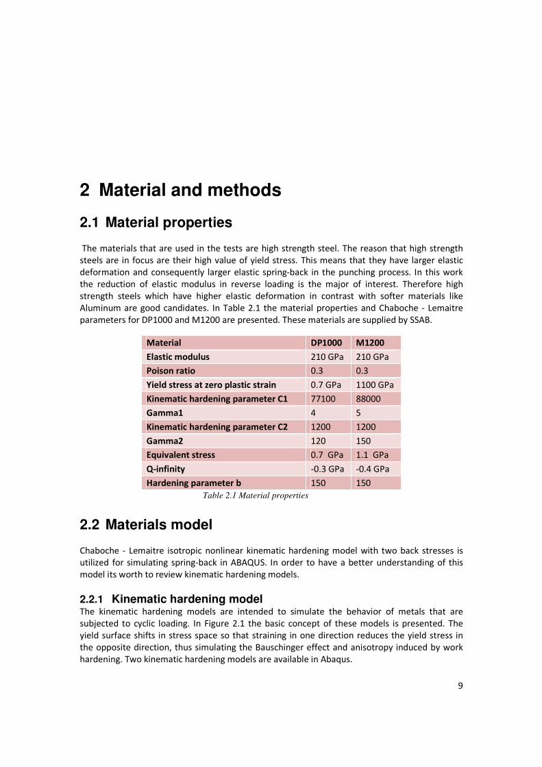
2.1 Material properties

The materials that are used in the tests are high strength steel. The reason that high strength

steels are in focus are their high value of yield stress. This means that they have larger elastic

deformation and consequently larger elastic spring-back in the punching process. In this work

the reduction of elastic modulus in reverse loading is the major of interest. Therefore high

strength steels which have higher elastic deformation in contrast with softer materials like

Aluminum are good candidates. In Table 2.1 the material properties and Chaboche - Lemaitre

parameters for DP1000 and M1200 are presented. These materials are supplied by SSAB.

2.2 Materials model

Chaboche - Lemaitre isotropic nonlinear kinematic hardening model with two back stresses is

utilized for simulating spring-back in ABAQUS. In order to have a better understanding of this

model its worth to review kinematic hardening models.

2.2.1 Kinematic hardening model The kinematic hardening models are intended to simulate the behavior of metals that are

subjected to cyclic loading. In Figure 2.1 the basic concept of these models is presented. The

yield surface shifts in stress space so that straining in one direction reduces the yield stress in

the opposite direction, thus simulating the Bauschinger effect and anisotropy induced by work

hardening. Two kinematic hardening models are available in Abaqus.

Material DP1000 M1200

Elastic modulus 210 GPa 210 GPa

Poison ratio 0.3 0.3

Yield stress at zero plastic strain 0.7 GPa 1100 GPa

Kinematic hardening parameter C1 77100 88000

Gamma1 4 5

Kinematic hardening parameter C2 1200 1200

Gamma2 120 150

Equivalent stress 0.7 GPa 1.1 GPa

Q-infinity -0.3 GPa -0.4 GPa

Hardening parameter b 150 150

Table 2.1 Material properties

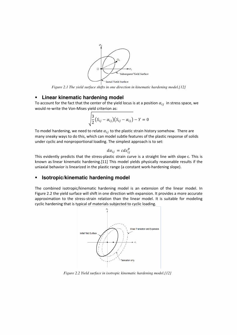
Figure 2.1 The yield surface shifts in one direction in kinematic hardening model.[12]

� Linear kinematic hardening model To account for the fact that the center of the yield locus is at a position �� in stress space, we

would re-write the Von-Mises yield criterion as:

!32 #�� $#�� $ � % � 0

To model hardening, we need to relate �� to the plastic strain history somehow. There are

many sneaky ways to do this, which can model subtle features of the plastic response of solids

under cyclic and nonproportional loading. The simplest approach is to set:

�� (��

This evidently predicts that the stress-plastic strain curve is a straight line with slope c. This is known as linear kinematic hardening.[11] This model yields physically reasonable results if the

uniaxial behavior is linearized in the plastic range (a constant work-hardening slope).

� Isotropic/kinematic hardening model

The combined isotropic/kinematic hardening model is an extension of the linear model. In Figure 2.2 the yield surface will shift in one direction with expansion. It provides a more accurate

approximation to the stress-strain relation than the linear model. It is suitable for modeling

cyclic hardening that is typical of materials subjected to cyclic loading.

Figure 2.2 Yield surface in isotropic kinematic hardening model.[12]

11

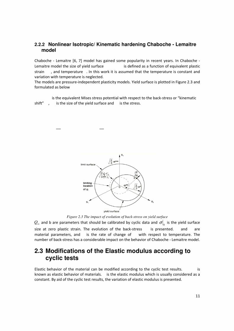
2.2.2 Nonlinear Isotropic/ Kinematic hardening Chaboche - Lemaitre model

Chaboche - Lemaitre [6, 7] model has gained some popularity in recent years. In Chaboche -

Lemaitre model the size of yield surface is defined as a function of equivalent plastic

strain , and temperature . In this work it is assumed that the temperature is constant and

variation with temperature is neglected.

The models are pressure-independent plasticity models. Yield surface is plotted in Figure 2.3 and

formulated as below

is the equivalent Mises stress potential with respect to the back-stress or “kinematic

shift” , is the size of the yield surface and is the stress.

Figure 2.3 The impact of evolution of back-stress on yield surface

and b are parameters that should be calibrated by cyclic data and 0

σ is the yield surface

size at zero plastic strain. The evolution of the back-stress is presented. and are

material parameters, and is the rate of change of with respect to temperature. The number of back-stress has a considerable impact on the behavior of Chaboche - Lemaitre model.

2.3 Modifications of the Elastic modulus according to cyclic tests

Elastic behavior of the material can be modified according to the cyclic test results. is

known as elastic behavior of materials. is the elastic modulus which is usually considered as a constant. By aid of the cyclic test results, the variation of elastic modulus is presented.

∞Q

),(0 θεσ pl

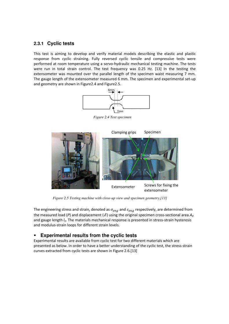
2.3.1 Cyclic tests This test is aiming to develop and verify material models describing the elastic and plastic

response from cyclic straining. Fully reversed cyclic tensile and compressive tests were

performed at room temperature using a servo-hydraulic mechanical testing machine. The tests

were run in total strain control. The test frequency was 0.25 Hz. [13] In the testing the

extensometer was mounted over the parallel length of the specimen waist measuring 7 mm.

The gauge length of the extensometer measured 6 mm. The specimen and experimental set-up

and geometry are shown in Figure2.4 and Figure2.5.

The engineering stress and strain, denoted as � )* and � )* respectively, are determined from

the measured load (P) and displacement (δ ) using the original specimen cross-sectional area A0

and gauge length l0. The materials mechanical response is presented in stress-strain hysteresis and modulus-strain loops for different strain levels.

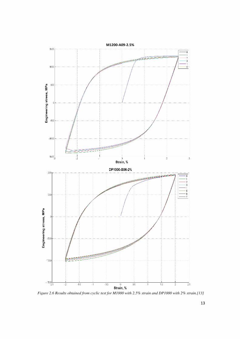
� Experimental results from the cyclic tests Experimental results are available from cyclic test for two different materials which are

presented as below. In order to have a better understanding of the cyclic test, the stress-strain

curves extracted from cyclic tests are shown in Figure 2.6.[13]

Extensometer

Specimen Clamping grips

Screws for fixing the

extensometer

Figure 2.5 Testing machine with close-up view and specimen geometry.[13]

Figure 2.4 Test specimen

6mm

7mm

13

M1200-A09-2.5%

Figure 2.6 Results obtained from cyclic test for M1000 with 2.5% strain and DP1000 with 2% strain.[13]

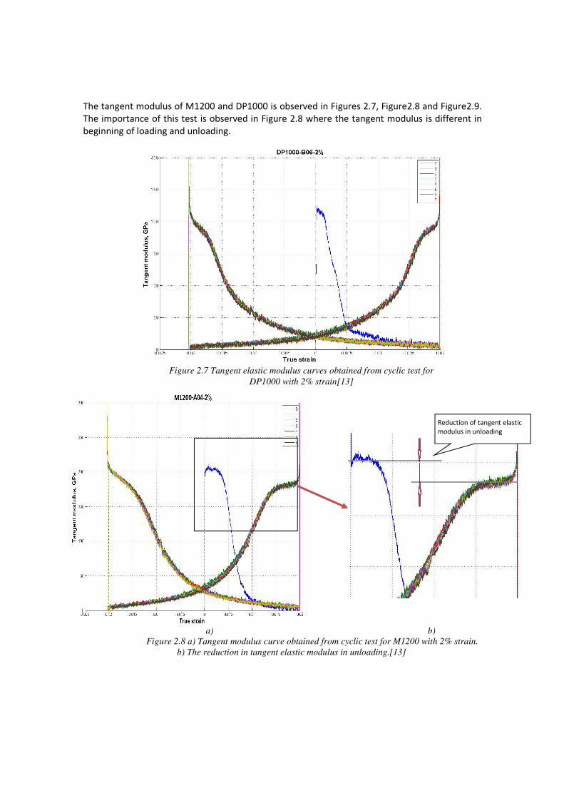
The tangent modulus of M1200 and DP1000 is observed in Figures 2.7, Figure2.8 and Figure2.9.

The importance of this test is observed in Figure 2.8 where the tangent modulus is different in

beginning of loading and unloading.

Figure 2.7 Tangent elastic modulus curves obtained from cyclic test for

DP1000 with 2% strain[13]

a) b)

Figure 2.8 a) Tangent modulus curve obtained from cyclic test for M1200 with 2% strain.

b) The reduction in tangent elastic modulus in unloading.[13]

Reduction of tangent elastic modulus in unloading

15

M1200-A09-2.5%

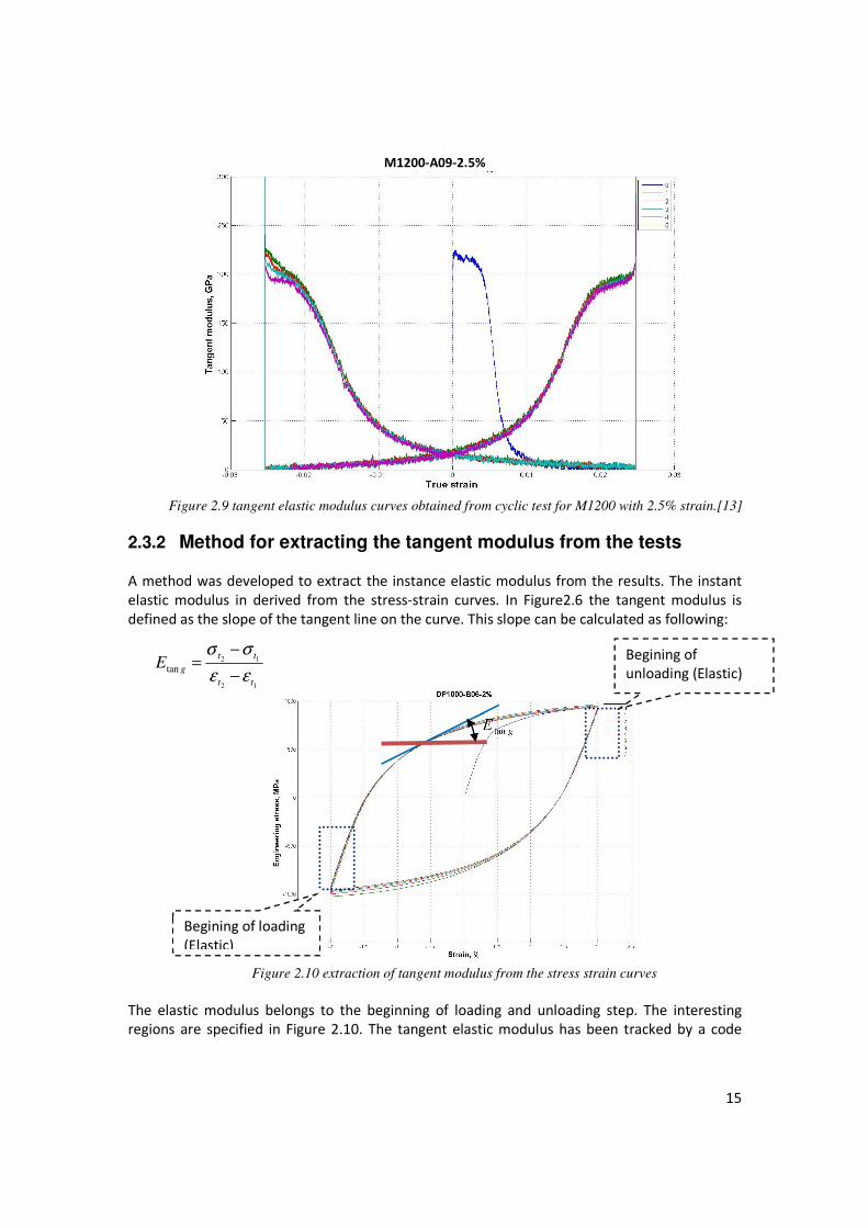
2.3.2 Method for extracting the tangent modulus from the tests A method was developed to extract the instance elastic modulus from the results. The instant

elastic modulus in derived from the stress-strain curves. In Figure2.6 the tangent modulus is

defined as the slope of the tangent line on the curve. This slope can be calculated as following:

Figure 2.10 extraction of tangent modulus from the stress strain curves

The elastic modulus belongs to the beginning of loading and unloading step. The interesting regions are specified in Figure 2.10. The tangent elastic modulus has been tracked by a code

Begining of unloading (Elastic)

Begining of loading

(Elastic)

12

12

tan

tt

tt

gEεε

σσ

−

−=

Figure 2.9 tangent elastic modulus curves obtained from cyclic test for M1200 with 2.5% strain.[13]

(Appendix 2) in the desired region. This code produces two different elastic modulus for each

cycle.

2.3.3 Short Discussion of instant Young’s modulus results By observing the instant elastic modulus it is concluded that for the tested materials, the

tangent modulus in the beginning of each cycle (elastic region) is not constant. Figure2.8.b

depicts a considerable reduction in tangent modulus in the beginning of compression step. The

exact reason for this behavior is not completely clear and several assumption has been made

which has is discussed in the introduction chapter. There are more experimental results with

different methods of testing have proven this phenomenon.[3]

2.4 Implementing the modified material modulus in ABAQUS by aid of USDFLD

The cyclic tests results show a variation in elastic modulus in deferent loading steps. In this part

it is aimed to implement this behavior in FEM codes.

2.4.1 Introduction to FEM

Finite Element Analysis was first developed in the early 1960's as a simulation and design tool in

the aerospace and nuclear industries where the safety of structures was critical. FEM, or Finite

Element Method, is a mathematical technique used to predict the response of structures and

materials to environmental factors [10 ]. Finite Element Analysis (FEA) uses FEM, as a powerful

engineering tool, to numerically simulate the real world without the need to test prototypes in a

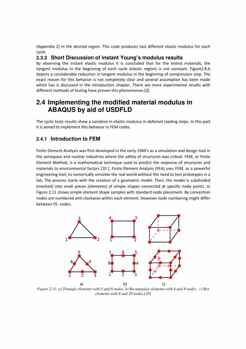
lab. The process starts with the creation of a geometric model. Then, the model is subdivided

(meshed) into small pieces (elements) of simple shapes connected at specific node points. In

Figure 2.11 shows simple element shape samples with standard node placement. By convention

nodes are numbered anti-clockwise within each element. However node numbering might differ

between FE- codes.

a) b) c)

Figure 2.11: a) Triangle elements with 3 and 6 nodes. b) Rectangular elements with 4 and 8 nodes. c) Box

elements with 8 and 20 nodes.[10]

17

The variation of displacement is assumed to be determined by simple polynomial shape

functions and nodal displacements. Equations for the strains and stresses are developed in

terms of the unknown nodal displacements. From this, the equations of equilibrium are

assembled in a matrix which can be easily programmed and solved on a computer. After

applying the appropriate boundary conditions, the nodal displacements are found by solving the matrix stiffness equation. Once the nodal displacements are known, element stresses and

strains can be calculated.

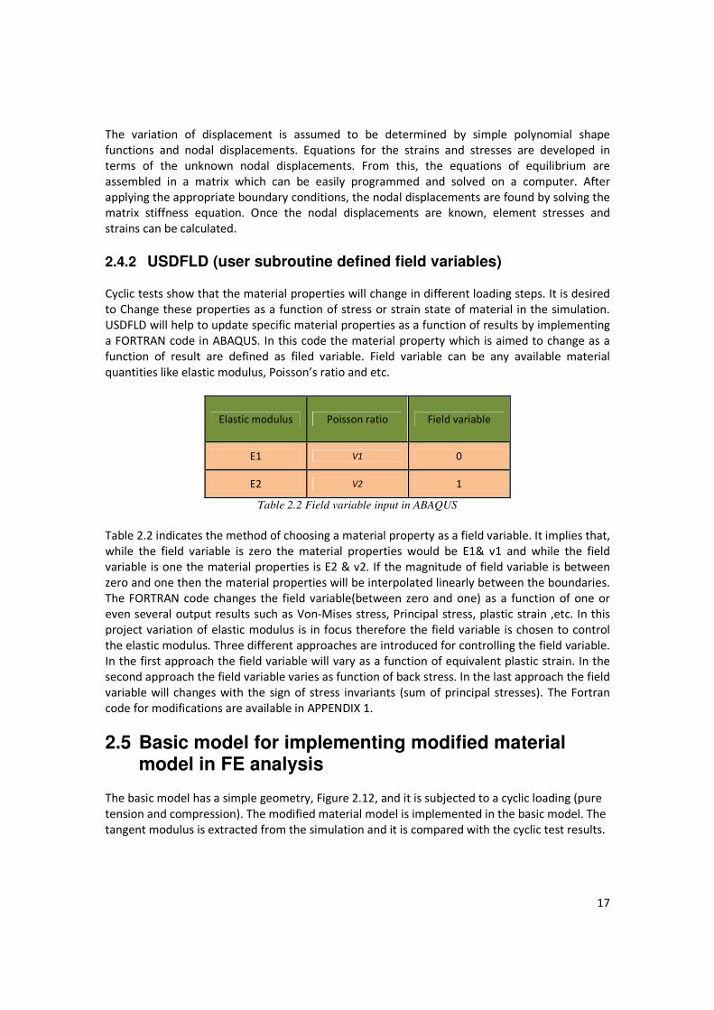
2.4.2 USDFLD (user subroutine defined field variables) Cyclic tests show that the material properties will change in different loading steps. It is desired

to Change these properties as a function of stress or strain state of material in the simulation.

USDFLD will help to update specific material properties as a function of results by implementing

a FORTRAN code in ABAQUS. In this code the material property which is aimed to change as a

function of result are defined as filed variable. Field variable can be any available material

quantities like elastic modulus, Poisson’s ratio and etc.

Elastic modulus Poisson ratio Field variable

E1 V1 0

E2 V2 1

Table 2.2 Field variable input in ABAQUS

Table 2.2 indicates the method of choosing a material property as a field variable. It implies that,

while the field variable is zero the material properties would be E1& v1 and while the field

variable is one the material properties is E2 & v2. If the magnitude of field variable is between

zero and one then the material properties will be interpolated linearly between the boundaries.

The FORTRAN code changes the field variable(between zero and one) as a function of one or

even several output results such as Von-Mises stress, Principal stress, plastic strain ,etc. In this

project variation of elastic modulus is in focus therefore the field variable is chosen to control

the elastic modulus. Three different approaches are introduced for controlling the field variable.

In the first approach the field variable will vary as a function of equivalent plastic strain. In the

second approach the field variable varies as function of back stress. In the last approach the field

variable will changes with the sign of stress invariants (sum of principal stresses). The Fortran

code for modifications are available in APPENDIX 1.

2.5 Basic model for implementing modified material model in FE analysis

The basic model has a simple geometry, Figure 2.12, and it is subjected to a cyclic loading (pure

tension and compression). The modified material model is implemented in the basic model. The

tangent modulus is extracted from the simulation and it is compared with the cyclic test results.

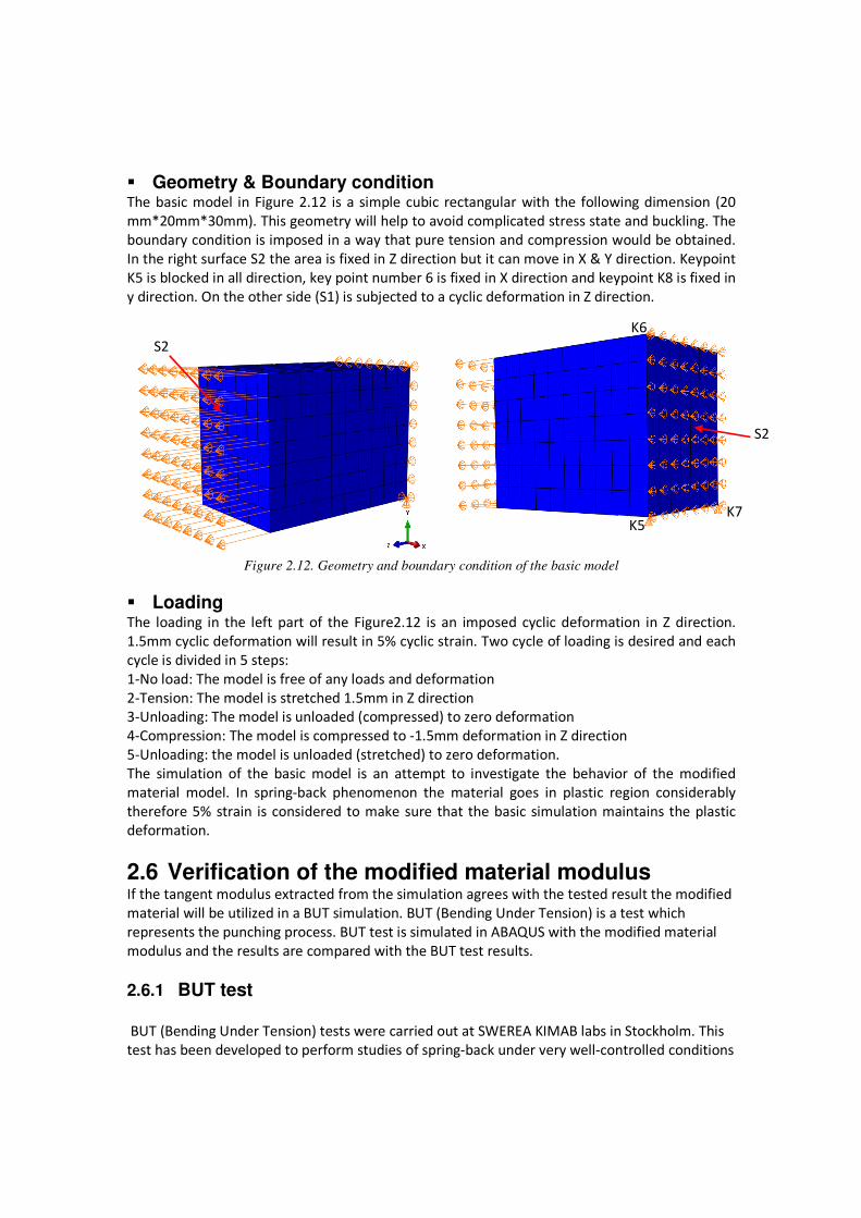
� Geometry & Boundary condition The basic model in Figure 2.12 is a simple cubic rectangular with the following dimension (20

mm*20mm*30mm). This geometry will help to avoid complicated stress state and buckling. The

boundary condition is imposed in a way that pure tension and compression would be obtained.

In the right surface S2 the area is fixed in Z direction but it can move in X & Y direction. Keypoint

K5 is blocked in all direction, key point number 6 is fixed in X direction and keypoint K8 is fixed in

y direction. On the other side (S1) is subjected to a cyclic deformation in Z direction.

Figure 2.12. Geometry and boundary condition of the basic model

� Loading The loading in the left part of the Figure2.12 is an imposed cyclic deformation in Z direction.

1.5mm cyclic deformation will result in 5% cyclic strain. Two cycle of loading is desired and each

cycle is divided in 5 steps:

1-No load: The model is free of any loads and deformation

2-Tension: The model is stretched 1.5mm in Z direction 3-Unloading: The model is unloaded (compressed) to zero deformation

4-Compression: The model is compressed to -1.5mm deformation in Z direction

5-Unloading: the model is unloaded (stretched) to zero deformation.

The simulation of the basic model is an attempt to investigate the behavior of the modified

material model. In spring-back phenomenon the material goes in plastic region considerably

therefore 5% strain is considered to make sure that the basic simulation maintains the plastic

deformation.

2.6 Verification of the modified material modulus If the tangent modulus extracted from the simulation agrees with the tested result the modified

material will be utilized in a BUT simulation. BUT (Bending Under Tension) is a test which

represents the punching process. BUT test is simulated in ABAQUS with the modified material

modulus and the results are compared with the BUT test results.

2.6.1 BUT test

BUT (Bending Under Tension) tests were carried out at SWEREA KIMAB labs in Stockholm. This

test has been developed to perform studies of spring-back under very well-controlled conditions

K5 K7

S2

S2

K6

19

and deliver repeatable test data regarding forces and geometry for subsequent modeling of

spring-back for the tested material.

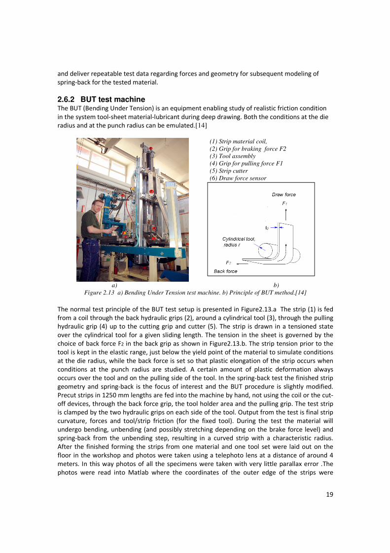
2.6.2 BUT test machine The BUT (Bending Under Tension) is an equipment enabling study of realistic friction condition

in the system tool-sheet material-lubricant during deep drawing. Both the conditions at the die radius and at the punch radius can be emulated.[14]

(1) Strip material coil,

(2) Grip for braking force F2

(3) Tool assembly

(4) Grip for pulling force F1

(5) Strip cutter

(6) Draw force sensor

a) b)

Figure 2.13 a) Bending Under Tension test machine. b) Principle of BUT method.[14]

The normal test principle of the BUT test setup is presented in Figure2.13.a The strip (1) is fed

from a coil through the back hydraulic grips (2), around a cylindrical tool (3), through the pulling hydraulic grip (4) up to the cutting grip and cutter (5). The strip is drawn in a tensioned state

over the cylindrical tool for a given sliding length. The tension in the sheet is governed by the

choice of back force F2 in the back grip as shown in Figure2.13.b. The strip tension prior to the

tool is kept in the elastic range, just below the yield point of the material to simulate conditions

at the die radius, while the back force is set so that plastic elongation of the strip occurs when

conditions at the punch radius are studied. A certain amount of plastic deformation always

occurs over the tool and on the pulling side of the tool. In the spring-back test the finished strip

geometry and spring-back is the focus of interest and the BUT procedure is slightly modified.

Precut strips in 1250 mm lengths are fed into the machine by hand, not using the coil or the cut-

off devices, through the back force grip, the tool holder area and the pulling grip. The test strip is clamped by the two hydraulic grips on each side of the tool. Output from the test is final strip

curvature, forces and tool/strip friction (for the fixed tool). During the test the material will

undergo bending, unbending (and possibly stretching depending on the brake force level) and

spring-back from the unbending step, resulting in a curved strip with a characteristic radius.

After the finished forming the strips from one material and one tool set were laid out on the

floor in the workshop and photos were taken using a telephoto lens at a distance of around 4

meters. In this way photos of all the specimens were taken with very little parallax error .The

photos were read into Matlab where the coordinates of the outer edge of the strips were

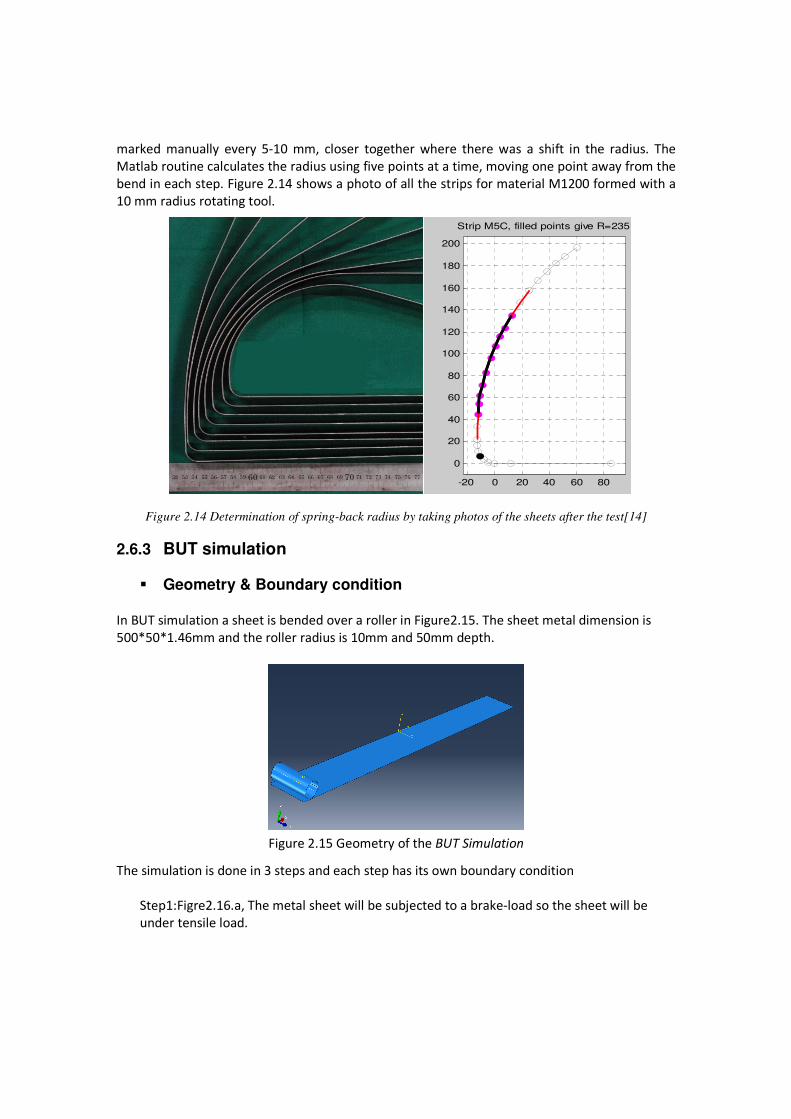
marked manually every 5-10 mm, closer together where there was a shift in the radius. The

Matlab routine calculates the radius using five points at a time, moving one point away from the

bend in each step. Figure 2.14 shows a photo of all the strips for material M1200 formed with a

10 mm radius rotating tool.

Figure 2.14 Determination of spring-back radius by taking photos of the sheets after the test[14]

2.6.3 BUT simulation

� Geometry & Boundary condition

In BUT simulation a sheet is bended over a roller in Figure2.15. The sheet metal dimension is

500*50*1.46mm and the roller radius is 10mm and 50mm depth.

The simulation is done in 3 steps and each step has its own boundary condition

Step1:Figre2.16.a, The metal sheet will be subjected to a brake-load so the sheet will be

under tensile load.

-20 0 20 40 60 80

0

20

40

60

80

100

120

140

160

180

200

Strip M5C, filled points give R=235

Figure 2.15 Geometry of the BUT Simulation

21

a) b) c)

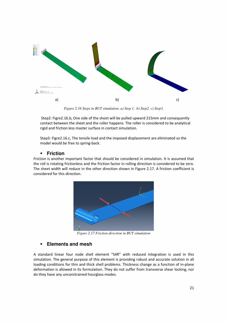
Figure 2.16 Steps in BUT simulation. a) Step 1. b) Step2. c) Step3.

Step2: Figre2.16.b, One side of the sheet will be pulled upward 215mm and consequently

contact between the sheet and the roller happens. The roller is considered to be analytical

rigid and friction less master surface in contact simulation.

Step3: Figre2.16.c, The tensile load and the imposed displacement are eliminated so the

model would be free to spring-back.

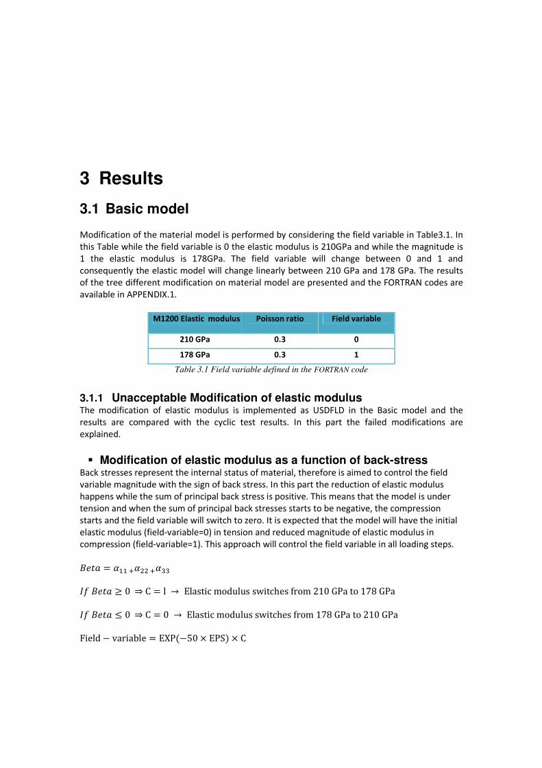
� Friction Friction is another important factor that should be considered in simulation. It is assumed that

the roll is rotating frictionless and the friction factor in rolling direction is considered to be zero.

The sheet width will reduce in the other direction shown in Figure 2.17. A friction coefficient is

considered for this direction.

� Elements and mesh

A standard linear four node shell element “S4R” with reduced integration is used in this

simulation. The general purpose of this element is providing robust and accurate solution in all

loading conditions for thin and thick shell problems. Thickness change as a function of in-plane deformation is allowed in its formulation. They do not suffer from transverse shear locking, nor

do they have any unconstrained hourglass modes.

Figure 2.17 Friction direction in BUT simulation

3 Results

3.1 Basic model

Modification of the material model is performed by considering the field variable in Table3.1. In

this Table while the field variable is 0 the elastic modulus is 210GPa and while the magnitude is

1 the elastic modulus is 178GPa. The field variable will change between 0 and 1 and

consequently the elastic model will change linearly between 210 GPa and 178 GPa. The results

of the tree different modification on material model are presented and the FORTRAN codes are

available in APPENDIX.1.

M1200 Elastic modulus Poisson ratio Field variable

210 GPa 0.3 0

178 GPa 0.3 1

Table 3.1 Field variable defined in the FORTRAN code

3.1.1 Unacceptable Modification of elastic modulus The modification of elastic modulus is implemented as USDFLD in the Basic model and the

results are compared with the cyclic test results. In this part the failed modifications are

explained.

� Modification of elastic modulus as a function of back-stress

Back stresses represent the internal status of material, therefore is aimed to control the field

variable magnitude with the sign of back stress. In this part the reduction of elastic modulus

happens while the sum of principal back stress is positive. This means that the model is under

tension and when the sum of principal back stresses starts to be negative, the compression

starts and the field variable will switch to zero. It is expected that the model will have the initial

elastic modulus (field-variable=0) in tension and reduced magnitude of elastic modulus in

compression (field-variable=1). This approach will control the field variable in all loading steps.

+�,- � ��.�//.�00 12+�,- 3 0 ⇒ C � l → Elasticmodulusswitchesfrom210GPato178GPa 12+�,- K 0 ⇒ C � 0 → Elasticmodulusswitchesfrom178GPato210GPa Field � variable � EXP��50 � EPS� � C

23

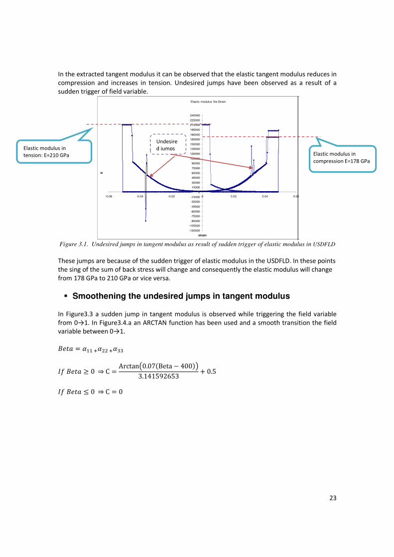
In the extracted tangent modulus it can be observed that the elastic tangent modulus reduces in

compression and increases in tension. Undesired jumps have been observed as a result of a

sudden trigger of field variable.

Figure 3.1. Undesired jumps in tangent modulus as result of sudden trigger of elastic modulus in USDFLD

These jumps are because of the sudden trigger of elastic modulus in the USDFLD. In these points

the sing of the sum of back stress will change and consequently the elastic modulus will change

from 178 GPa to 210 GPa or vice versa.

� Smoothening the undesired jumps in tangent modulus In Figure3.3 a sudden jump in tangent modulus is observed while triggering the field variable

from 0→1. In Figure3.4.a an ARCTAN function has been used and a smooth transition the field variable between 0→1.

+�,- � ��.�//.�00

12+�,- 3 0 ⇒ C � Arctan#0.07�Beta � 400�$3.141592653 � 0.5

12+�,- K 0 ⇒ C � 0

Elastic modulus Via Strain

-120000

-105000

-90000

-75000

-60000

-45000

-30000

-15000

0

15000

30000

45000

60000

75000

90000

105000

120000

135000

150000

165000

180000

195000

210000

225000

240000

-0.06 -0.04 -0.02 0 0.02 0.04 0.06

strain

E

Elastic modulus in

tension: E=210 GPa Elastic modulus in

compression E=178 GPa

Undesired jumps

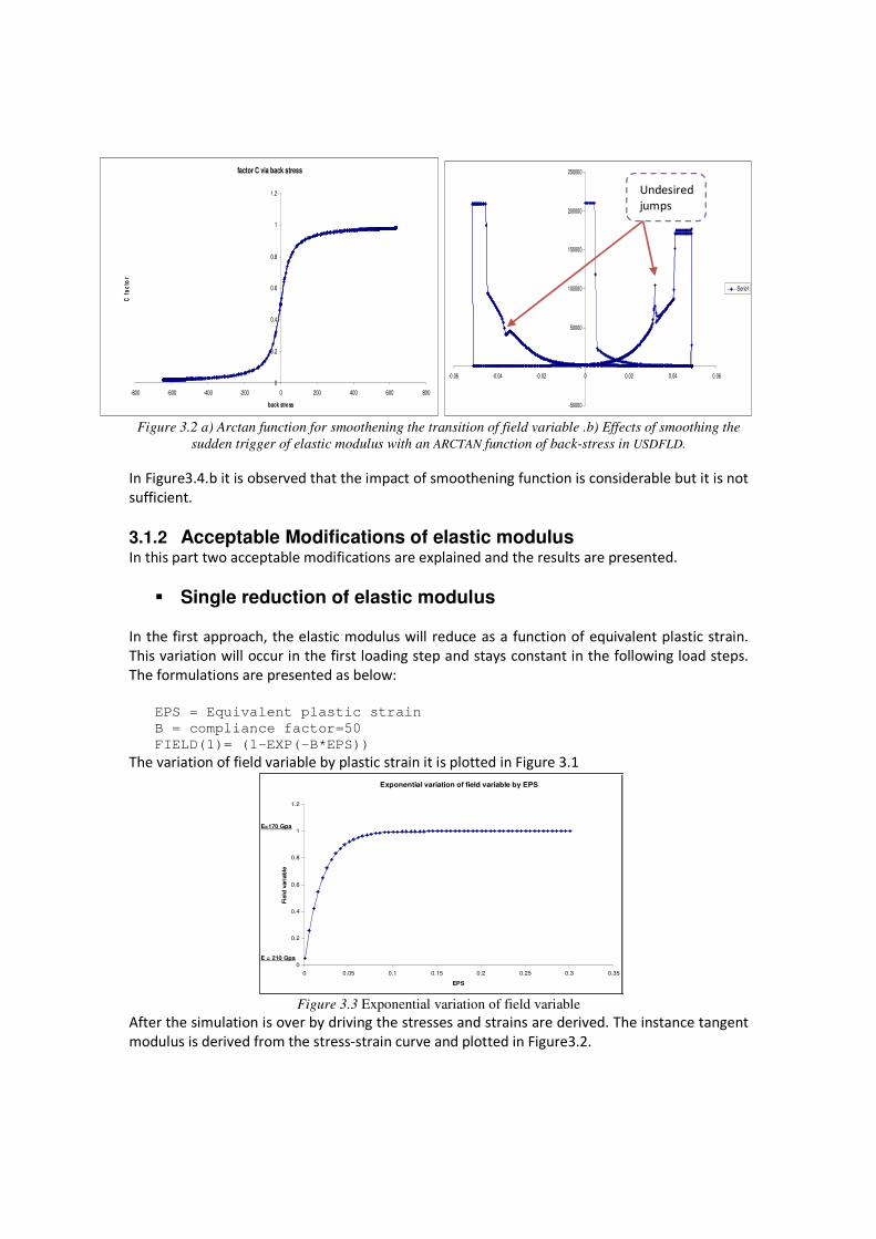
Figure 3.2 a) Arctan function for smoothening the transition of field variable .b) Effects of smoothing the

sudden trigger of elastic modulus with an ARCTAN function of back-stress in USDFLD.

In Figure3.4.b it is observed that the impact of smoothening function is considerable but it is not

sufficient.

3.1.2 Acceptable Modifications of elastic modulus In this part two acceptable modifications are explained and the results are presented.

� Single reduction of elastic modulus

In the first approach, the elastic modulus will reduce as a function of equivalent plastic strain.

This variation will occur in the first loading step and stays constant in the following load steps.

The formulations are presented as below:

EPS = Equivalent plastic strain

B = compliance factor=50

FIELD(1)= (1-EXP(-B*EPS))

The variation of field variable by plastic strain it is plotted in Figure 3.1

Figure 3.3 Exponential variation of field variable

After the simulation is over by driving the stresses and strains are derived. The instance tangent

modulus is derived from the stress-strain curve and plotted in Figure3.2.

factor C via back stress

0

0.2

0.4

0.6

0.8

1

1.2

-800 -600 -400 -200 0 200 400 600 800

back stress

C f

ac

tor

-50000

0

50000

100000

150000

200000

250000

-0.06 -0.04 -0.02 0 0.02 0.04 0.06

Serie1

Exponential variation of field variable by EPS

0

0.2

0.4

0.6

0.8

1

1.2

0 0.05 0.1 0.15 0.2 0.25 0.3 0.35

EPS

Fie

ld v

ari

ab

le

E=170 Gpa

E = 210 Gpa

Undesired

jumps

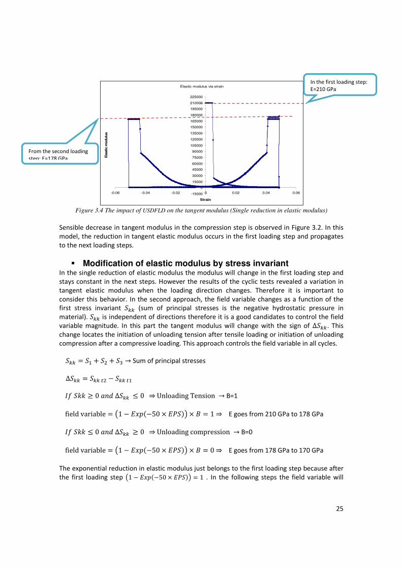
25

Figure 3.4 The impact of USDFLD on the tangent modulus (Single reduction in elastic modulus)

Sensible decrease in tangent modulus in the compression step is observed in Figure 3.2. In this

model, the reduction in tangent elastic modulus occurs in the first loading step and propagates

to the next loading steps.

� Modification of elastic modulus by stress invariant In the single reduction of elastic modulus the modulus will change in the first loading step and

stays constant in the next steps. However the results of the cyclic tests revealed a variation in

tangent elastic modulus when the loading direction changes. Therefore it is important to

consider this behavior. In the second approach, the field variable changes as a function of the first stress invariant �YY (sum of principal stresses is the negative hydrostatic pressure in

material). �YY is independent of directions therefore it is a good candidates to control the field

variable magnitude. In this part the tangent modulus will change with the sign of ∆�YY. This

change locates the initiation of unloading tension after tensile loading or initiation of unloading

compression after a compressive loading. This approach controls the field variable in all cycles. �YY � �� / � �0 → Sum of principal stresses

∆�YY � �YY[/ � �YY[� 12�\\ 3 0-]�∆�YY K 0 ⇒UnloadingTension → B=1

fieldvariable � #1 � ab��50 � c��$ � + � 1 ⇒ E goes from 210 GPa to 178 GPa

12�\\ K 0-]�∆�YY 3 0 ⇒Unloadingcompression → B=0

fieldvariable � #1 � ab��50 � c��$ � + � 0 ⇒ E goes from 178 GPa to 170 GPa

The exponential reduction in elastic modulus just belongs to the first loading step because after

the first loading step #1 � ab��50 � c��$ � 1 . In the following steps the field variable will

Elastic modulus via strain

-15000

0

15000

30000

45000

60000

75000

90000

105000

120000

135000

150000

165000

180000

195000

210000

225000

-0.06 -0.04 -0.02 0 0.02 0.04 0.06

Strain

Ela

stic m

odulu

s

From the second loading

step: E=178 GPa

In the first loading step:

E=210 GPa

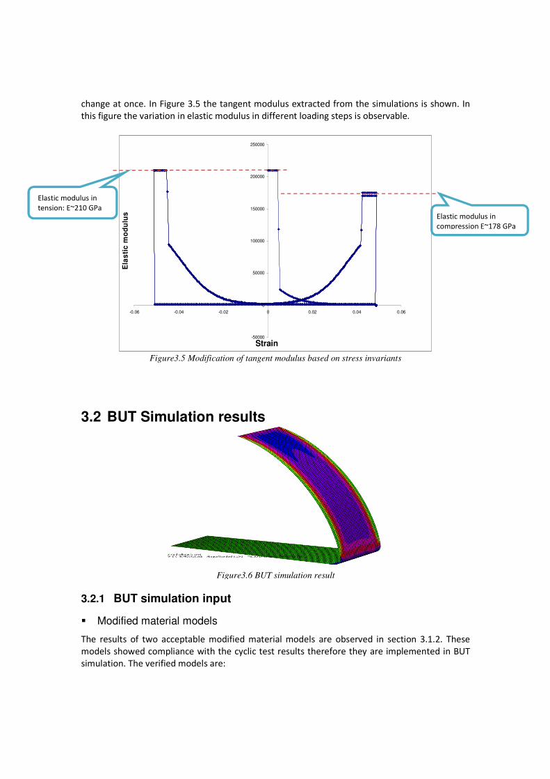
change at once. In Figure 3.5 the tangent modulus extracted from the simulations is shown. In

this figure the variation in elastic modulus in different loading steps is observable.

Figure3.5 Modification of tangent modulus based on stress invariants

3.2 BUT Simulation results

3.2.1 BUT simulation input

� Modified material models

The results of two acceptable modified material models are observed in section 3.1.2. These

models showed compliance with the cyclic test results therefore they are implemented in BUT

simulation. The verified models are:

-50000

0

50000

100000

150000

200000

250000

-0.06 -0.04 -0.02 0 0.02 0.04 0.06

Strain

Ela

sti

c m

od

ulu

s

Figure3.6 BUT simulation result

Elastic modulus in

tension: E~210 GPa Elastic modulus in

compression E~178 GPa

27

� Single reduction in elastic modulus

� Modification on elastic modulus by stress invariants

� Elastic modulus extracted from the cyclic tests

The magnitudes of elastic modulus extracted from the cyclic tests are presented in Table 3.2

Material Elastic modulus

in tension

Elastic modulus

in compression

DP1000 210 GPa 187.443 GPa

M1200 210 GPa 178.011 GPa

� Brake force

BUT test is bending under tension. In this test a sheet is subjected to a tension before bending

which are called brake forces. Table 3.3 three different brake forces for each material are

presented.

Brake force (KN)

Material 1 2 3

DP1000 29.5 41.3 53.1 M1200 49.5 55.1 64.3

� Coefficient of friction

The impact of friction on spring-back profile is in focus in this work. In section 2.6.3 it is

mentioned that the roll is rotating frictionless in the bending direction. Therefore a friction

coefficient should be considered in the orthogonal direction to the rolling direction. In BUT

simulation the roll is rolling frictionless and an orthotropic friction is considered. The orthotropic

friction allows considering friction coefficient in both directions in future works. The friction

coefficients that are obtained in KIMAB laboratory are presented in Table 3.4

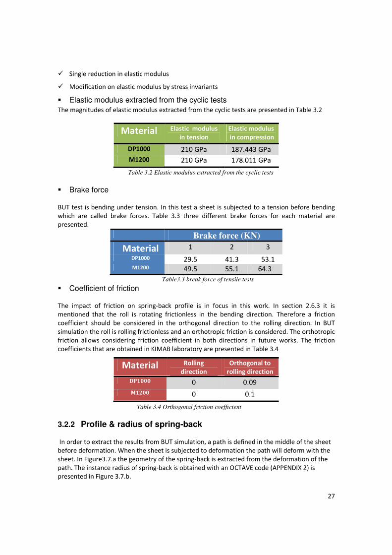
3.2.2 Profile & radius of spring-back

In order to extract the results from BUT simulation, a path is defined in the middle of the sheet

before deformation. When the sheet is subjected to deformation the path will deform with the

sheet. In Figure3.7.a the geometry of the spring-back is extracted from the deformation of the

path. The instance radius of spring-back is obtained with an OCTAVE code (APPENDIX 2) is

presented in Figure 3.7.b.

Table 3.2 Elastic modulus extracted from the cyclic tests

Table3.3 break force of tensile tests

Material Rolling

direction

Orthogonal to

rolling direction

DP1000 0 0.09

M1200 0 0.1

Table 3.4 Orthogonal friction coefficient

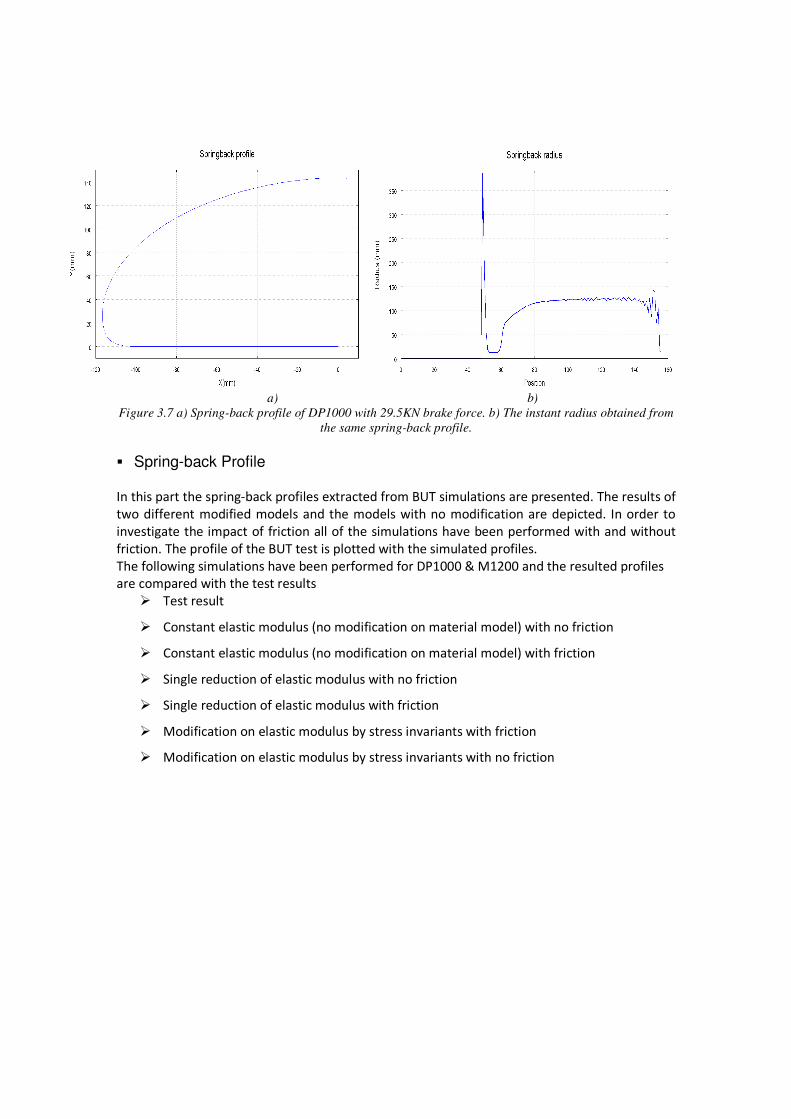
a) b)

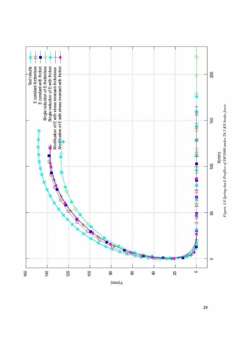
Figure 3.7 a) Spring-back profile of DP1000 with 29.5KN brake force. b) The instant radius obtained from

the same spring-back profile.

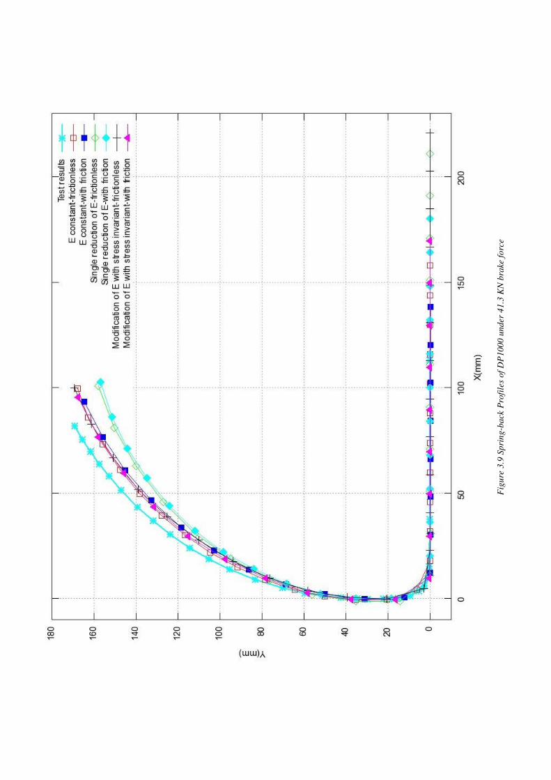
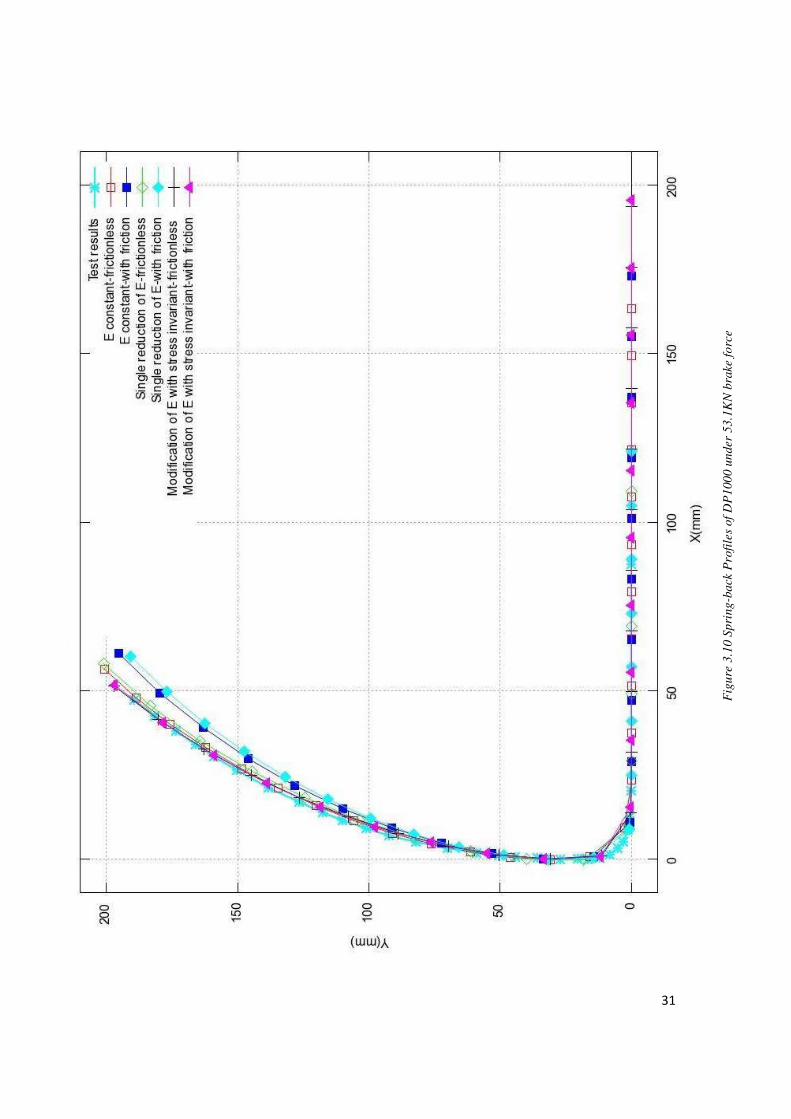
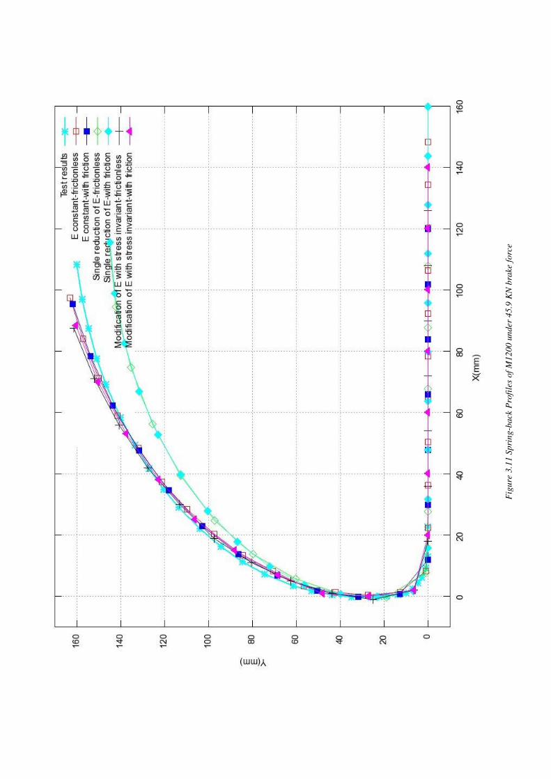
� Spring-back Profile

In this part the spring-back profiles extracted from BUT simulations are presented. The results of

two different modified models and the models with no modification are depicted. In order to

investigate the impact of friction all of the simulations have been performed with and without

friction. The profile of the BUT test is plotted with the simulated profiles.

The following simulations have been performed for DP1000 & M1200 and the resulted profiles are compared with the test results

� Test result

� Constant elastic modulus (no modification on material model) with no friction

� Constant elastic modulus (no modification on material model) with friction

� Single reduction of elastic modulus with no friction

� Single reduction of elastic modulus with friction

� Modification on elastic modulus by stress invariants with friction

� Modification on elastic modulus by stress invariants with no friction

29

Fig

ure

3.8

Spri

ng-b

ack P

rofi

les

of

DP

10

00 u

nder

29.5

KN

bra

ke f

orc

e

Fig

ure

3.9

Spri

ng-b

ack P

rofi

les

of

DP

100

0 u

nder

41.3

KN

bra

ke f

orc

e

31

Fig

ure

3.1

0 S

pri

ng-b

ack P

rofi

les

of

DP

100

0 u

nder

53.1

KN

bra

ke f

orc

e

Fig

ure

3.1

1 S

pri

ng-b

ack P

rofi

les

of

M1

200 u

nder

45.9

KN

bra

ke f

orc

e

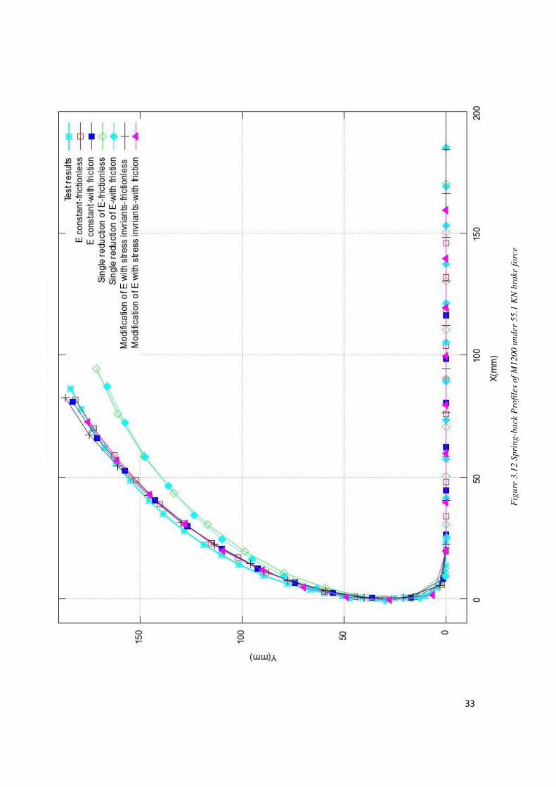
33

Fig

ure

3.1

2 S

pri

ng-b

ack P

rofi

les

of

M1

200 u

nder

55.1

KN

bra

ke f

orc

e

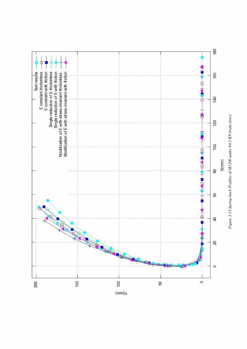
Fig

ure

3.1

3 S

pri

ng-b

ack P

rofi

les

of

M1

200 u

nder

64.3

KN

bra

ke f

orc

e

35

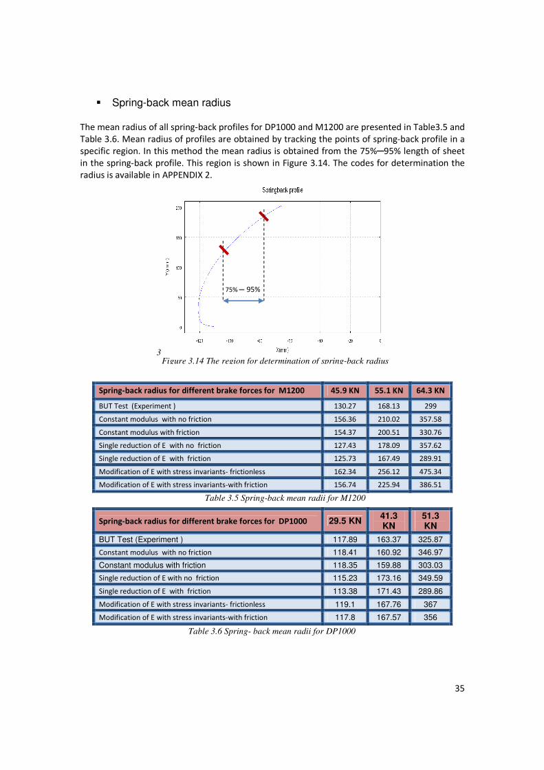
� Spring-back mean radius

The mean radius of all spring-back profiles for DP1000 and M1200 are presented in Table3.5 and

Table 3.6. Mean radius of profiles are obtained by tracking the points of spring-back profile in a

specific region. In this method the mean radius is obtained from the 75%─95% length of sheet

in the spring-back profile. This region is shown in Figure 3.14. The codes for determination the

radius is available in APPENDIX 2.

3

Spring-back radius for different brake forces for M1200 45.9 KN 55.1 KN 64.3 KN

BUT Test (Experiment ) 130.27 168.13 299

Constant modulus with no friction 156.36 210.02 357.58

Constant modulus with friction 154.37 200.51 330.76

Single reduction of E with no friction 127.43 178.09 357.62

Single reduction of E with friction 125.73 167.49 289.91

Modification of E with stress invariants- frictionless 162.34 256.12 475.34

Modification of E with stress invariants-with friction 156.74 225.94 386.51

Spring-back radius for different brake forces for DP1000 29.5 KN 41.3 KN

51.3 KN

BUT Test (Experiment ) 117.89 163.37 325.87

Constant modulus with no friction 118.41 160.92 346.97

Constant modulus with friction 118.35 159.88 303.03

Single reduction of E with no friction 115.23 173.16 349.59

Single reduction of E with friction 113.38 171.43 289.86

Modification of E with stress invariants- frictionless 119.1 167.76 367

Modification of E with stress invariants-with friction 117.8 167.57 356

Table 3.5 Spring-back mean radii for M1200

Table 3.6 Spring- back mean radii for DP1000

75% ─ 95%

Figure 3.14 The region for determination of spring-back radius

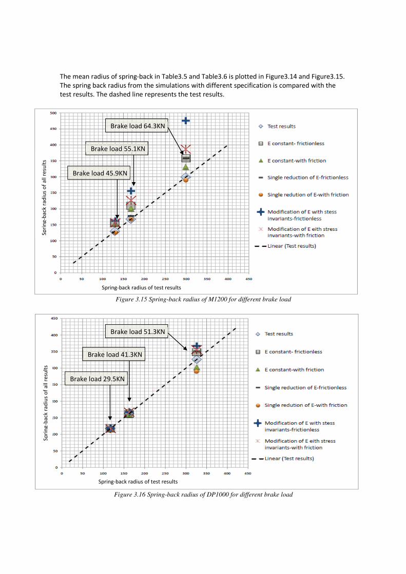
The mean radius of spring-back in Table3.5 and Table3.6 is plotted in Figure3.14 and Figure3.15.

The spring back radius from the simulations with different specification is compared with the

test results. The dashed line represents the test results.

Figure 3.15 Spring-back radius of M1200 for different brake load

Figure 3.16 Spring-back radius of DP1000 for different brake load

Brake load 45.9KN

Brake load 55.1KN

Brake load 64.3KN

Brake load 29.5KN

Brake load 41.3KN

Brake load 51.3KN

Spring-back radius of test results

Spri

ng-

bac

k ra

diu

s o

f al

l re

sult

s

Spri

ng-

bac

k ra

diu

s o

f al

l re

sult

s

Spring-back radius of test results

37

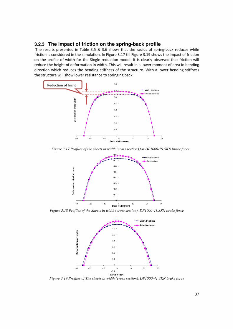
3.2.3 The impact of friction on the spring-back profile The results presented in Table 3.5 & 3.6 shows that the radius of spring-back reduces while friction is considered in the simulation. In Figure 3.17 till Figure 3.19 shows the impact of friction

on the profile of width for the Single reduction model. It is clearly observed that friction will

reduce the height of deformation in width. This will result in a lower moment of area in bending

direction which reduces the bending stiffness of the structure. With a lower bending stiffness

the structure will show lower resistance to springing back.

Figure 3.18 Profiles of the Sheets in width (cross section). DP1000-41.3KN brake force

Figure 3.19 Profiles of The sheets in width (cross section). DP1000-41.3KN brake force

Figure 3.17 Profiles of the sheets in width (cross section) for DP1000-29.5KN brake force

Reduction of hight

4 Discussion

4.1 Overview Predicting spring-back magnitude of deformed strips after a forming process is in focus in this

thesis. Previous efforts for simulating this process revealed deviations in spring-back magnitude

from the tested results.[3, 8] The impact of micro plastic phenomenon in metals during forming

process is one of the possible reasons for these deviations. This phenomenon results in a

variation of elastic modulus especially in high strength steel during the process. We modified

material models to consider micro plastic behaviors of metals in Simulating forming process.

Friction is another important factor in the forming process. All simulations are performed with

and without considering friction and the results are compared with the test results.

We modified the material models based on cyclic test results. This test had been performed on

different material in KIMAB laboratory in order to investigate the behavior of material in cyclic

loading. If a load cycle is divided into four steps (Tension, Unloading tension, Compression,

Unloading compression) The tangent modulus extracted from these tests shows a variation in

elastic modulus during different steps.[12] This behavior was observed in previous investigations

by Cleveland and Ghosh [3] and R. Cobo et al [8]. It is assumed that the deviation of results in

simulation and tests is due to variation of elastic modulus in different steps of a load cycle.

Nonlinear isotropic-kinematic hardening Chaboche model has been used in simulating the

forming process. Three different modifications are performed on the elastic modulus by aid of USDFLD (user defined subroutines field variable) in ABAQUS. These modifications have no effect

on the plastic behavior of the material. The modified material models are checked by simulating

a simple geometry subjected to a cyclic loading. The behavior of the tangent modulus extracted

from these simulations and cyclic tests are compared. Two of the modifications had satisfactory

compliance with the test result. The first modification is named single reduction of elastic

modulus and results in a reduction of elastic modulus as a function of equivalent plastic strain.

In this modification the reduction of elastic modulus in the first loading step propagates to the

next steps. Second modification is named modification of elastic modulus by stress invariants

and results in reduction of elastic modulus in definite steps in a load cycle (unloading tension, compression). This modification is a function of equivalent plastic strain and first stress invariant

(sum of principal stresses). Both of the modifications are implemented in simulating BUT test.

BUT (Bending under tension) test was performed at KIMAB laboratory and represented the

stamping process.

Impact of friction is another factor that is investigated in this work. Considering friction provides

more realistic simulations. We performed all of the simulations with and without considering

friction and the results are compared with the test results.

39

4.2 Conclusion

4.2.1 Impact of friction The results depict a considerable reduction in spring-back radius in all simulations while friction

is considered. This reduction is due to the deformation of width. In Figure3.17, 3.18 and 3.19, it

is observed that friction reduces the height of deformation in width and consequently the moment of area will reduce in bending direction. This means that friction will reduce the

bending stiffness of the strip and the strip will have a larger spring-back (lower radius will be

obtained).

4.2.2 First modification (single reduction of elastic modulus) The first modified material model (single reduction of elastic modulus) has made a large

improvement in predicting the spring-back magnitude. In M1200 where the reduction of elastic modulus is large, the improvement of spring-back prediction is considerable. The first

modification with friction has made the best prediction in M1200. For DP1000 the model with

no modification and with friction made the best prediction of spring-back.

4.2.3 Second modification (modification of elastic modulus by stress invariants)

In the second modification shows deviations from the test results and the results are not

reliable. One of the possible reasons of these deviations is the data extracted from the cyclic

tests. In cyclic tests the behavior of tangent modulus is recorded for 2% strain and all

modifications are based on these results. However the strain magnitude in BUT test is larger and

there might be unknown behavior of materials in strains larger than 2%.

4.3 Future work The materials property plays the major role in spring back simulation. In the cyclic tests, the

strain range is 2%. In the forming process the strain range is much higher than 2% and

depending on the forming process it could be more than 10% therefore extrapolating the

material properties of 2% strain to the real forming strain is not reliable. Performing tests that provides us with material properties in a higher strain range is a great help in simulating Spring-

back phenomenon.

More material modifications can be performed based on tested result. Modifications based on

back-stress are very interested because back-stress shows the material status and the position

of yield surface in the material model.

5 References

[1] Baba, A., Tozawa, Y., 1964. Effect of tensile force in stretch-forming

process on the springback. Bulletin of the JSME 7, 835–843.

[2] Wong, T.E., Johnson, G.C., 1988. On the effects of elastic nonlinearity in

metals. Transactions of the ASME 110, 332–337.

[3] R.M.Cleveland, A.K. Ghosh ” Inelastic effects on springback in metals”

Int. J.of plast,18(2002),769-785

[4] Stout, M.G., Rollett, A.D., 1990. Large-strain Bauschinger effects in fcc

metals and alloys. Met. Trans. A21A, 3201–3213.

[5] S. L. Zang ,J. Liang, C. Guo , international Jornal of Machine Tools

&Manufacture 47 (2007) 1791-1797

[6] J. Lemaitre, J.L. Chaboche - Lemaitre, Mechanics of Solid Materials,

Cambridge University Press, Cambridge, 1990.

[7] J.L. Chaboche - Lemaitre, Constitutive equations for cyclic plasticity and

cyclic visco-plasticity, International Journal of Plasticity 5 (1989) 247.

[8] R.cobo,M. pla ,r. Hernandez and J.A. beneto. Aanalysis of the decrease of

the apparent young’s modulus of advanced high strength steels and it’s

effect in bending simulation

[9] [L.J. Vin, A.H. Streppl, U.P. Singh, A process model for air bending, Journal

of Materials Processing Technology 56 (1996) 48–54.]

[10] http://www.wceng-fea.com

[11] http://www.engin.brown.edu/courses/en222/Notes/plasticity/plasticity

.htm

41

[12] http://tnodiana.com/node/369

[13] E. Sjöström. Reversed cyclic strain controlled testing, Swerea KIMAB,

225021 Sprincom, 2011-05-20.

[14] Springback tests in the BUT (Bending under tension) machine at KIMAB,

2010-07-02

6 Appendix � Apendix1

FORTRAN codes for modification of material model

- FORTRAN code for single reduction in elastic modulus SUBROUTINE USDFLD(FIELD,STATEV,PNEWDT,DIRECT,T,CELENT,

1 TIME,DTIME,CMNAME,ORNAME,NFIELD,NSTATV,NOEL,NPT,LAYER,

2 KSPT,KSTEP,KINC,NDI,NSHR,COORD,JMAC,JMATYP,MATLAYO,

3 LACCFLA)

INCLUDE 'ABA_PARAM.INC'

CHARACTER*80 CMNAME,ORNAME

CHARACTER*3 FLGRAY(15)

DIMENSION FIELD(NFIELD),STATEV(NSTATV),DIRECT(3,3),

1 T(3,3),TIME(2)

DIMENSION ARRAY(15),JARRAY(15),JMAC(*),JMATYP(*),

1 COORD(*)

C Absolute value of current strain:

CALL GETVRM('PE',ARRAY,JARRAY,FLGRAY,JRCD,JMAC,JMATYP,

1 MATLAYO,LACCFLA)

EPS = ARRAY(7)

C In this part the field variable will change from 0 to 1

FIELD(1)= (1-EXP(-50*EPS))

C If error, write comment to .DAT file:

IF(JRCD.NE.0)THEN

WRITE(6,*) 'REQUEST ERROR IN USDFLD FOR ELEMENT NUMBER ',

1 NOEL,'INTEGRATION POINT NUMBER ',NPT

ENDIF

RETURN

END

- FORTRAN code for cyclic variation of elastic modulus as a function of back stress

SUBROUTINE USDFLD(FIELD,STATEV,PNEWDT,DIRECT,T,CELENT, 1 TIME,DTIME,CMNAME,ORNAME,NFIELD,NSTATV,NOEL,NPT,LAYER,


43

3 LACCFLA)





1 T(3,3),TIME(2)


1 COORD(*)



1 MATLAYO,LACCFLA)

EPS = ARRAY(7)

CALL GETVRM('ALPHA',ARRAY,JARRAY,FLGRAY,JRCD,JMAC,JMATYP,

1 MATLAYO,LACCFLA)

C Extracting three back stress from the simulation

Alfa1=ARRAY(1)

Alfa2=ARRAY(2)

Alfa3=ARRAY(3)

Beta =Alfa1+Alfa2+Alfa3

C Changing the field variable as a function of sign of the sum of back

stress

if (Beta < 0) then

C=0

ELSE

C=1

ENDIF

WRITE(6,*) 'Beta',Beta

FIELD(1)= (1-EXP(-50*EPS))*c

C Store the maximum strain as a solution dependent state variable

STATEV(1)= FIELD(1)


IF(JRCD.NE.0)THEN



ENDIF

RETURN

END

- FORTRAN code for cyclic modification with back stress (Smoothening with ArCTAN function)

SUBROUTINE USDFLD(FIELD,STATEV,PNEWDT,DIRECT,T,CELENT,



3 LACCFLA)

C


C




1 T(3,3),TIME(2)


1 COORD(*)



1 MATLAYO,LACCFLA)

EPS = ARRAY(7)

CALL GETVRM('ALPHA',ARRAY,JARRAY,FLGRAY,JRCD,JMAC,JMATYP,

1 MATLAYO,LACCFLA)

C Extracting three back stress from the simulation

Alfa1=ARRAY(1)

Alfa2=ARRAY(2)

Alfa3=ARRAY(3)

Beta =Alfa1+Alfa2+Alfa3

C Changing the field variable as a function of sign of the sum of back

stress

if (Beta < 0) then

C=0

ELSE

C=(ATAN(0.07*(Beta-400))/(3.141592653)+0.5)

ENDIF

FIELD(1)= (1-EXP(-50*EPS))*C

C Store the maximum strain as a solution dependent state

C variable

STATEV(1) = FIELD(1)


IF(JRCD.NE.0)THEN



ENDIF

C

RETURN

END

- FORTRAN code for cyclic modification as a function of stress invariants

SUBROUTINE USDFLD(FIELD,STATEV,PNEWDT,DIRECT,T,CELENT,



45

3 LACCFLA)

C


C




1 T(3,3),TIME(2)


1 COORD(*)

C



1 MATLAYO,LACCFLA)

EPS = ARRAY(7)

C

CALL GETVRM('S',ARRAY,JARRAY,FLGRAY,JRCD,JMAC,JMATYP,

1 MATLAYO,LACCFLA)

S1=ARRAY(1)

S2=ARRAY(2)

S3=ARRAY(3)

St=S1+S2+S3

EPS_old=STATEV(1)

St_old=STATEV(2)

St_saved=STATEV(3)

D= St-St_old

if(((St>0).and.(D<0)).or.((St<0).and.(D>0)))then

St_saved=St

end if

delta_peeq = EPS - EPS_old

delta_St = (St-St_saved)

IF(delta_peeq==0)then

if (St>0) then

B=1

Else

B=0

End IF

ENDif

if ((St_old==St_saved).and.(abs(delta_st )>300 ))then

if (St>0) then

B=1

Else

B=0

End IF

End IF

C WRITE(6,*) 'PEEQ',EPS

C WRITE(6,*) 'S3',S3

C hear the fild variable will change fromm 0 to 1

FIELD(1)= (1-EXP(-50*EPS))*B

c to varable is stored in the state variable to save the amont of the

previous number

STATEV(1)=EPS

STATEV(2)=St

STATEV(3)=Stsaved


IF(JRCD.NE.0)THEN



ENDIF

C

RETURN

END

47

� APENDIX2

Octave code for extracting results from tests and simulation

- Octave code for extracting elastic modulus from cyclic tests % SprinCon Docol 1000

% Första skarpa provstaven

clear all

clc

a=load('Anew.txt');

Q =length(a)

f=zeros(Q,1);

anew=[];

A=10.44e-6

nk=1;

for i=1:Q

if abs(a(i,2))<0.02

anew=[anew;a(i,1)/A a(i,2)];

nk=nk+1;

else

f(nk,1)=1;

endif

end

r=find(f(:,1)==1);

rlen=length(r);

for i = 1:rlen

dF=anew(r(i)+10,1)-anew(r(i),1);

de=anew(r(i)+10,2)-anew(r(i),2);

E(i)=dF/de;

end

DP1000Modulus=E'

- Octave code for extraction of the instant elastic from the simulation

clear all

clc

%load EVNOFRIC.txt

%load EVFRI.txt

%load ECFRIC.txt

% old kimab simulation radius extraction

load M1200.txt

kim=M1200(2:3:128,:);

for t3=1:length(kim)-3;

v31=[kim(:,5)-kim(:,4) kim(:,6)];

x1=v31(t3,1);x2=v31(t3+1,1);x3=v31(t3+2,1);

y1=v31(t3,2);y2=v31(t3+1,2);y3=v31(t3+2,2);

x12 = x1-x2;

y12 = y1-y2;

x13 = x1-x3;

y13 = y1-y3;

d = x12*y13 - x13*y12;

%Test for collinear points:

if abs(d) > 0;

r12 = x12*(x1+x2) + y12*(y1+y2);

r13 = x13*(x1+x3) + y13*(y1+y3);

a = 0.5*r12/d;

b = 0.5*r13/d;

%Compute center and radius:

x0 = a*y13 - b*y12;

y0 = -a*x13 + b*x12;

r31(t3) = sqrt((x1-x0)^2 + (y1-y0)^2);

if r31(t3) < 5000;

r311(t3)=sqrt((x1-x0)^2 + (y1-y0)^2);

end

end

end

Figure(1)

plot(r311,'-c','LineWidth',2)

title('Spring-back radius old kim','fontsize',25)

%axis([0 50 0 1000])

grid on

xlabel('Position','FontSize',20)

ylabel('Radius (mm)','FontSize',20)

rq1=30:38;

mean(r311(rq1));

print 'Spring-back radius old kim.jpg'

Rm_oldkim= mean(r311(rq1))

investigation and implementation of non- …511820/fulltext01.pdf · investigation and...

Documents