INVESTIGATING THE RELIABILITY OF ULTRASOUND PHASED ARRAY

METHOD AND CONVENTIONAL ULTRASONIC TESTING FOR

DETECTION OF DEFECTS IN AUSTENITIC STAINLESS STEELS

A THESIS SUBMITTED TO

THE GRADUATE SCHOOL OF NATURAL AND APPLIED SCIENCES

OF

MIDDLE EAST TECHNICAL UNIVERSITY

BY

BAHADIR AKGÜN

IN PARTIAL FULFILLMENT OF THE REQUIREMENTS

FOR

THE DEGREE OF MASTER OF SCIENCE

IN

METALLURGICAL AND MATERIALS ENGINEERING

AUGUST 2015

Approval of the thesis:

INVESTIGATING THE RELIABILITY OF ULTRASOUND PHASED

ARRAY METHOD AND CONVENTIONAL ULTRASONIC TESTING FOR

DETECTION OF DEFECTS IN AUSTENITIC STAINLESS STEELS

Submitted by BAHADIR AKGÜN in partial fulfillment of the requirements for the

degree of Master of Science in Metallurgical and Materials Engineering

Department, Middle East Technical University by,

Prof. Dr. Gülbin Dural Ünver _______________

Dean, Graduate School of Natural and Applied Sciences

Prof. Dr. C. Hakan Gür _______________

Head of Department, Metallurgical and Materials Engineering

Prof. Dr. C. Hakan Gür _______________

Supervisor, Metallurgical and Materials Eng. Dept., METU

Examining Committee Members:

……………………………………………… ……………………

……………………………………………… ……………………

……………………………………………… ……………………

……………………………………………… ……………………

……………………………………………… ……………………

Date: 07.08.2015

iv

I hereby declare that all information in this document has been obtained and

presented in accordance with academic rules and ethical conduct. I also declare

that, as required by these rules and conduct, I have fully cited and referenced all

material and results that are not original to this work.

Name, Last name: Bahadır AKGÜN

Signature:

v

ABSTRACT

INVESTIGATING THE RELIABILITY OF ULTRASOUND PHASED ARRAY

METHOD AND CONVENTIONAL ULTRASONIC TESTING FOR

DETECTION OF DEFECTS IN AUSTENITIC STAINLESS STEELS

AKGÜN, Bahadır

M.S., Department of Metallurgical and Materials Engineering

Supervisor: Prof. Dr. C. Hakan GÜR

August 2015, 111 pages

In recent years Phased Array (PA) method has become an alternative to the

conventional ultrasonic method for critical tests in aerospace, oil, gas and nuclear

industries. There is a challenge for inspection of austenitic stainless steels due to high

attenuation, skewing and scattering of sound beam. The aim of this thesis is to

investigate and to compare the flaw detection abilities of conventional ultrasonic and

PA systems using the probability of detection (PoD) approach for testing of austenitic

stainless steel blocks and weldments having both artificial and natural defects. Grain

size, micro hardness, attenuation measurements, radioscopic and macroscopic

inspections were also performed. Three types of test blocks were prepared from AISI

304 steel. First specimen is the block having ø2 mm side drilled holes at different

depths; second specimen has side drilled holes with varying diameters between 0.5 to

5 mm at the same depth; and the third specimen is the welded plate having both

artificial and natural defects. Although PA method has automated calibration, beam

focusing and steering abilities, the PoD analyses did not show remarkable advantage

of PA for detecting artificial flaws, except those in the surface near zone. On the

welded specimen, however, the PA inspection is clearly more successful than

conventional method based on counts of detected flaw possibilities as well as

positioning and sizing of the defects. While the automated PA system has superior

vi

detection and positioning abilities over the manual PA system, the manual PA system

has superiority of faster scanning and swiveling of the probe which also brings the risk

of human factor.

Keywords: Ultrasonic Testing; Phased Array; Probability of Detection (PoD).

vii

ÖZ

ÖSTENİTİK PASLANMAZ ÇELİKLERDE FAZ DİZİSİ VE GELENEKSEL

ULTRASONİK TEST METOTLARININ HATA TESPİT

KABİLİYETLERİNİN KARŞILAŞTIRILMASI

AKGÜN, Bahadır

Yüksek Lisans, Metalurji ve Malzeme Mühendisliği Bölümü

Tez Yöneticisi: Prof. Dr. C. Hakan GÜR

Ağustos 2015, 111 sayfa

Son yıllarda Faz Dizi ( PA ) yöntemi havacılık, petrol, gaz ve nükleer

sektörlerinde kritik testler için geleneksel ultrasonik (UT) yönteme alternatif bir metot

haline gelmiştir. Östenitik paslanmaz çeliklerde ses zayıflamasının yüksek olması, ses

demetinin saçılması ve sapmasından dolayı östenitk paslanmaz çeliklerin ultrasonik

yöntemlerle muayenesi oldukça zordur. Bu tezin amacı, yapay hatalara sahip östenitik

paslanmaz çelik bloklar ile yapay ve doğal hataları barındıran kaynaklı plakada hata

tespit bulma olasılığı (PoD) yaklaşımını kullanarak geleneksel UT ve faz dizi PA

sistemlerinin hata tespit etme yeteneklerini karşılaştırmaktır. Ayrıca tane boyutu,

mikro sertlik, ses zayıflaması ölçümleri, radyoskopik ve makroskopik muayeneler

gerçekleştirilmiştir. 304 paslanmaz çelik olan üç tip test numunesi hazırlanmıştır. İlk

numune farklı derinliklerde Ø2 mm çapta delikler olan bloktur; ikinci numune delikleri

5 mm ile 0,5 arasında değişen çaplarda aynı derinlikte olan bloktur ve üçüncü numune

yapay ve kaynak hatalarını bulunduran kaynaklı plakadır. PA metodu otomatik

kalibrasyon, ses demeti odaklama ve ses demetini farklı zamanlarda ateşleyerek

kontrol edebilme özelliklerine rağmen, yapay hatalara sahip test bloklarında

gerçekleştirilen hata tespit analizlerinde (PoD) yüzeye en yakın hatayı bulmak dışında

büyük bir farklılık ortaya çıkarmamıştır. Fakat kaynaklı plakada yapılan muayenelerde

faz dizisi (PA) metodu hata tespit sayısı, hataları konumlandırma ve boyutlandırma

yönlerinden geleneksel UT yönteminden daha başarılıdır. Otomatik PA sistemi üstün

viii

algılama ve konumlandırma yetenekleri yönünden manuel PA sisteminden daha

başarılı olmasına rağmen, manuel PA sistemi daha hızlı tarama ve prob dönüşü

üstünlüğüne sahiptir fakat bu durum insan faktörü riskini de beraberinde getirmektedir.

Anahtar Sözcükler: Ultrasonik Test; Faz Dizisi; Hata Tespit Olasılığı (PoD).

ix

TABLE OF CONTENTS

ABSTRACT ................................................................................................................ v

ÖZ .............................................................................................................................. vii

TABLE OF CONTENTS .......................................................................................... ix

LIST OF FIGURES ................................................................................................ xiii

LIST OF TABLES ................................................................................................ xviii

CHAPTER 1 ............................................................................................................... 1

INTRODUCTION ...................................................................................................... 1

1.1 GENERAL .................................................................................................. 1

1.2 ULTRASONIC TESTING .......................................................................... 2

1.2.1 Introduction to Ultrasonic ................................................................... 2

1.2.2 Conventional Ultrasonic Inspection – Advantages and Disadvantages

............................................................................................................. 2

1.2.3 Physics of Ultrasound ......................................................................... 3

1.2.4 Major Variables in Ultrasonic Inspection ........................................... 4

1.2.5 Wave Propagation ............................................................................... 5

1.2.6 Mode Conversion and Snell’s Law ..................................................... 6

1.2.7 Attenuation of Sound Waves .............................................................. 9

1.2.8 Acoustic Impedance .......................................................................... 11

1.2.9 Reflection and Transmission Coefficients ........................................ 11

1.2.10 Wave Interaction or Interference ...................................................... 12

1.2.11 Wave Interference ............................................................................. 13

1.2.12 Ultrasonic Equipment and Transducers ............................................ 14

x

1.2.13 The Characteristics of Piezoelectric Transducers ............................. 15

1.2.14 Radiated Fields of Ultrasonic Transducers ....................................... 16

1.2.15 Beam Divergence and Beam Spread ................................................. 17

1.2.16 Ultrasonic Measurement Methods .................................................... 17

1.2.17 Data Presentation of Ultrasonic Testing ............................................ 20

1.3 PHASED ARRAY SYSTEM.................................................................... 21

1.3.1 Basic Principles of Phased Array ...................................................... 21

1.3.2 Phased Array Probe Characteristics .................................................. 23

1.3.3 Software Control and Phased Pulsing of Phased Array .................... 23

1.3.4 Beam Steering and Shaping .............................................................. 25

1.3.5 Beam Focusing with Phased Array Probes ....................................... 26

1.3.6 Application of Phased Array System ................................................ 27

1.4 Probability of Detection (PoD) Analysis .................................................. 30

1.5 Ultrasonic Inspection of Austenitic Stainless Steels ................................. 34

1.5.1 Symmetry of the Austenitic Weld Material ...................................... 38

1.5.2 Phase Velocity ................................................................................... 38

1.5.3 Polarization Vector ............................................................................ 42

1.6 Beam Distortion in Anisotropic Media ..................................................... 43

1.6.1 Beam Divergence .............................................................................. 43

1.6.2 Beam Skewing ................................................................................... 43

1.6.3 Beam Spreading Factor ..................................................................... 44

1.6.4 The effects of inhomogeneous austenitic weld metal on sound

propagation ........................................................................................................ 46

1.7 Modelling the grain orientation ................................................................. 47

1.7.1 Solidification Modes ......................................................................... 49

1.8 Motivation and Aim of the study .............................................................. 51

xi

CHAPTER 2 ............................................................................................................. 53

EXPERIMENTAL PROCEDURE ......................................................................... 53

2.1 Material and Sample Preparation .............................................................. 53

2.1.1 Specimen Type 1 (Flaws at Different Depths) .................................. 54

2.1.2 Specimen Type 2 (Flaws of Different Sizes at the Same Depth) ...... 55

2.1.3 Specimen Type 3 (Butt Welded Plate) .............................................. 55

2.2 Investigation of Microstructure ................................................................. 57

2.3 Ultrasonic Inspections (Specimen Type 1 and Type 2) ............................ 57

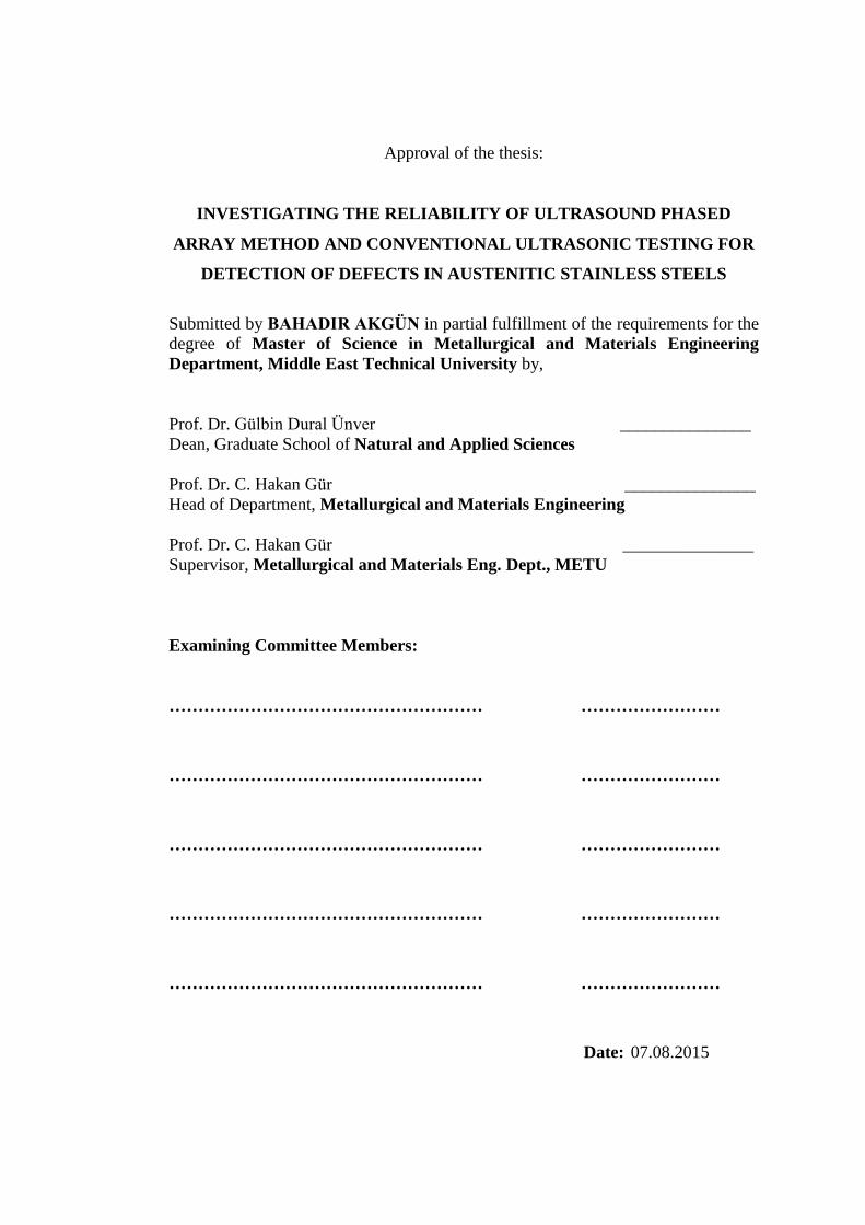
2.4 Phased Array Inspections (Specimens Type 1 and Type 2) ...................... 58

2.5 Ultrasonic inspections (Specimen Type 3 – The Butt Welded Plate) ....... 59

2.6 Automated Phased Array Inspections with Encoder (Specimen Type 3 –

The Butt Welded Plate) ......................................................................................... 62

2.7 Manual Phased Array Inspection on Butt Welded Plate (Specimen Type 3)

................................................................................................................... 69

2.8 Probability of Detection Analysis ............................................................. 71

CHAPTER 3 ............................................................................................................. 73

RESULTS AND DISCUSSION .............................................................................. 73

3.1 Microstructure ........................................................................................... 73

3.2 Results of Ultrasonic and Phased Array Inspections ................................ 77

3.3 Probability of Detection (PoD) Analysis .................................................. 81

3.3.1 a vs â Linear Model for PoD Analysis of Type 1 Specimen (UT) .... 81

3.3.2 a vs â Linear Model for PoD Analysis of Specimen Type 1 (PA) .... 83

3.3.3 PoD Analysis of Specimen Type 1 ................................................... 84

xii

3.3.4 PoD Analysis of Specimen Type 2 ................................................... 86

3.4 Evaluation of Manual Phased Array inspections ...................................... 89

3.5 Evaluation of Automated Phased Array Inspections ................................. 92

3.6 The radioscopy testing of the butt welded plate (specimen type 3) ........ 100

3.7 The macroscopic inspection of the butt welded plate (specimen type 3) 101

CHAPTER 4 ........................................................................................................... 103

CONCLUSION ....................................................................................................... 103

REFERENCES ....................................................................................................... 107

xiii

LIST OF FIGURES

Figure 1.1 The frequency range [1]............................................................................. 2

Figure 1.2 Sound velocities in various mediums [4]................................................... 3

Figure 1.3 Wavelength display [4] .............................................................................. 4

Figure 1.4 Longitudinal and transverse waves [4] ...................................................... 6

Figure 1.5 L-Wave and S-Wave schematic display [5] .............................................. 7

Figure 1.6 Refraction of waves [6] ............................................................................. 7

Figure 1.7 Snell’s Law correlation of velocity and refracted angle ............................ 8

Figure 1.8 Attenuation [9] ......................................................................................... 10

Figure 1.9 Transmission and refraction [4] ............................................................... 12

Figure 1.10 Phase interference [10] .......................................................................... 13

Figure 1.11 Wave interference [10] .......................................................................... 13

Figure 1.12 The piezoelectric transducers [4] ........................................................... 15

Figure 1.13 Variations of acoustic sound pressure with distance for circular crystal

[9] .............................................................................................................................. 16

Figure 1.14 Beam spread [4] ..................................................................................... 17

Figure 1.15 Transmission method [9] ....................................................................... 18

Figure 1.16 Signal presentation of the back wall ...................................................... 19

Figure 1.17 Signal presentation of the back wall and a defect ................................. 19

Figure 1.18 The back wall and B, C defect signal presentation [10] ........................ 20

Figure 1.19 A commercial Phased Array instrument [11] ........................................ 21

Figure 1.20 (On the left) a single transducer’s element, (on the right) a multi PA

transducers [12] ......................................................................................................... 22

Figure 1.21 Grouping of elements in the Phased Array probe [12] .......................... 23

xiv

Figure 1.22 Beam forming, time delay for pulsing, receiving multiple elements [15]

................................................................................................................................... 24

Figure 1.23 Beam focusing first normal longitudinal sound beam second shear wave

generation [15] .......................................................................................................... 24

Figure 1.24 Time delays on firing of Phased Array elements [15] ........................... 25

Figure 1.25 Conventional UT and PA probes [15] ................................................... 25

Figure 1.26 Beam focusing for different number of elements and apertures [11] .... 26

Figure 1.27 Phased Array A-scan, B-scan and C-scan respectively [13] ................. 27

Figure 1.28 Multiple image display [13] ................................................................... 28

Figure 1.29 A typical PoD process presentation [16] ............................................... 31

Figure 1.30 The publications dealing with PoD in the field of NDT [17] ................ 32

Figure 1.31 Signal Response versus Crack Depth [18] ............................................. 33

Figure 1.32 Isotropic and anisotropic phenomena in phased array method [30] ...... 35

Figure 1.33 Macro graphic view (a), domain model (b) [30] ................................... 36

Figure 1.34 Illustration of anisotropic reflection and transmission behavior of the

ultrasonic wave in testing of austenitic weld. ‘d’ represents the deviation between the

locations of the reflected signals for isotropic and anisotropic cases [33] ................ 37

Figure 1.35 Illustration of the interaction of an ultrasonic ray with transversal crack

in isotropic and anisotropic weld materials. ‘d’ represents the deviation between the

locations of reflected signal [33] ............................................................................... 37

Figure 1.36 Illustration of the transverse isotropic symmetry in austenitic welds

material [33] .............................................................................................................. 38

Figure 1.37 Coordinate system used to represent the three dimensional crystal

orientation of the transversal isotropic austenitic weld material. Ɵ represents the

columnar grain orientation and Ψ represents the layback orientation [33] ............... 39

xv

Figure 1.38 The columnar grain orientation in the austenitic steel is 90º. R: Raleigh

wave, H: Head wave, qSV: quasi shear vertical wave, qP: quasi longitudinal wave

[33] ............................................................................................................................ 39

Figure 1.39 Acoustic wave phase velocity surfaces in the isotropic steel material: a)

longitudinal wave and b) shear vertical wave [33] ................................................... 40

Figure 1.40 Phase velocity surfaces in the transversely isotropic austenitic stainless

steel (X6 Cr Ni 1811): a), d) quasi longitudinal waves, b), e) Shear horizontal waves

and c), f) quasi shear vertical waves [33] .................................................................. 41

Figure 1.41 Polarization vectors for the longitudinal (P) and shear vertical (SV)

waves in the isotropic steel [33] ................................................................................ 42

Figure 1.42 Polarization vectors for the quasi longitudinal (qP) and quasi shear

vertical (qSV) waves in the austenitic stainless steel (X6 CrNi 1811) with a) 0° and

b) 50°columnar grain orientation [33] ...................................................................... 42

Figure 1.43 Variation of beam skewing angle with incident wave vector angle for the

three wave modes in the columnar grained austenitic steel material. Ɵ represents the

columnar grain orientation and Ψ represents the layback orientation [33] ............... 44

Figure 1.44 Variation of beam spreading factor with incidence wave vector angle for

the three wave modes in the columnar grained austenitic steel material [33] .......... 45

Figure 1.45 A 45º ultrasonic beam propagation in the inhomogeneous austenitic weld

(a) Longitudinal waves (P), (b) shear vertical waves (SV) and (c) shear horizontal

waves (SH) [33] ........................................................................................................ 46

Figure 1.46 Weld macrographs; modelled orientations as vectors; contour plots of

differences between modelling and orientation by contour lines (0–10–20–30°) [36]

................................................................................................................................... 47

Figure 1.47 (On the left) Beam deviation and splitting in a weld with a transducer,

(on the right) example of simulated propagation using a grain orientation model to

describe material anisotropy [36] .............................................................................. 48

Figure 1.48 (a) planar; (b) cellular; (c) columnar dendritic; (d) equiaxed dendritic

[21] ............................................................................................................................ 49

xvi

Figure 1.49 Variations in temperature gradient G and growth rate R [21] ............... 50

Figure 1.50 Variation in solidification mode across the fusion zone [21] ................ 50

Figure 2.1 Specimen Type 1 ..................................................................................... 54

Figure 2.2 Specimen Type 2 ..................................................................................... 55

Figure 2.3 Weld bevel preparation with ES beam tool3 software ............................ 56

Figure 2.4 Manual Phased Array Equipment Sonotron Isonic 2010......................... 58

Figure 2.5 Sonotron Isonic 2010 PA Software ......................................................... 58

Figure 2.6 Calculation of sound path distance .......................................................... 59

Figure 2.7 DAC curve schematic presentation .......................................................... 61

Figure 2.8 Display of 2nd defect signal ...................................................................... 61

Figure 2.9 Phased Array testing apparatus – Olympus Omniscan MX .................... 62

Figure 2.10 ES Beam Tool3 probe configuration ..................................................... 62

Figure 2.11 Sectorial beam set configuration ............................................................ 63

Figure 2.12 Weld bevel image on the screen of Sonotron Isonic 2010 .................... 69

Figure 2.13 Manual Phased Array inspection ........................................................... 70

Figure 2.14 Defect list captured by Sonotron Isonic 2010 ........................................ 70

Figure 3.1 Representative micrographs for the specimen type 3 Parent, HAZ and

weld metal at (5 x) (a), Fusion line at (20 x) (b) ....................................................... 73

Figure 3.2 Micro hardness values versus distance to weld line ................................ 74

Figure 3.3 Four possible a vs â models for Type 1 specimen (UT) .......................... 81

Figure 3.4 a vs â linear models for specimen type 1 (UT) ........................................ 82

Figure 3.5 a vs â parameter values in UT [26] .......................................................... 83

Figure 3.6 a vs â linear model Specimen Type 1 (PA) ............................................. 84

Figure 3.7 PoD curve of specimen type 1 (UT) ........................................................ 85

Figure 3.8 PoD curve of specimen type 1 (PA) ........................................................ 85

xvii

Figure 3.9 PoD curve for Type 2 specimen (UT) ..................................................... 87

Figure 3.10 PoD curve for Type 2 specimen (PA).................................................... 87

Figure 3.11 The holes and slot on the specimen type 3 ............................................ 89

Figure 3.12 the Detected flaws list and schematic display of flaws-1 (MPA) .......... 90

Figure 3.13 The Detected flaws list and schematic display of flaws-2 (MPA) ........ 90

Figure 3.14 Meandering scan of the weld and swiveling of the probe [2]................ 91

Figure 3.15 The lack of fusion on manual PA display and destructive macro test ... 91

Figure 3.16 Evaluation of 1st data ............................................................................. 95

Figure 3.17 Evaluation of 2nd data ............................................................................ 95

Figure 3.18 Evaluation of 3rd data ............................................................................. 95

Figure 3.19 Evaluation of 4th data ............................................................................. 96

Figure 3.20 Evaluation of 5th data ............................................................................. 96

Figure 3.21 Evaluation of 6th data ............................................................................. 97

Figure 3.22 Evaluation of 7th data ............................................................................. 97

Figure 3.23 Evaluation of 8th data ............................................................................. 97

Figure 3.24 Evaluation of 9th and 10th data ............................................................... 98

Figure 3.25 Evaluation of 11th data ........................................................................... 98

Figure 3.26 Evaluation of 12th data ........................................................................... 99

Figure 3.27 Evaluation of 13th, 14th and 15th data ..................................................... 99

Figure 3.28 Radioscopic image of the specimen type 3 (200 kV) .......................... 100

Figure 3.29 Radiographic image of the specimen type 3 (200 kV) ........................ 101

Figure 3.30 The macroscopic image of the specimen type 3 .................................. 101

xviii

LIST OF TABLES

Table 1.1 Advantages and disadvantages of ultrasonic testing [2] ............................. 3

Table 1.2 Compressional and shear velocities in various materials [4] ...................... 4

Table 1.3 Change in the sound pressure .................................................................... 10

Table 1.4 Acoustic impedances (kg/m2s) of various media ...................................... 11

Table 1.5 The Correlation between beam steering and pitch size - elements ........... 26

Table 1.6 The essential variables of the Phased Array technique [14] ..................... 29

Table 2.1 Chemical composition of AISI 304 steel (Specimen type 3) .................... 53

Table 2.2 Chemical Composition of GMAW Solid Wire MG2 Weld Metal

(Specimen type 3) [39] .............................................................................................. 56

Table 2.3 Sp Calculations .......................................................................................... 59

Table 2.4 Phased array Omniscan MX software parameters ................................... 64

Table 2.5 Results of the first trial (10 mm focal depth) ............................................ 66

Table 2.6 Phased array Omniscan MX software parameters for the Second trial .... 67

Table 2.7 Results of the second trial no (25 mm focal depth) .................................. 68

Table 3.1 Grain sizes and mechanical values of the AISI 304 [25] .......................... 74

Table 3.2 Average attenuation in the columnar and equiaxed structure [28] ........... 75

Table 3.3 The mean attenuation values in the specimen type 1 and 2 (longitudinal

wave) ......................................................................................................................... 76

Table 3.4 The mean attenuation values in the columnar and equiaxed structure of the

specimen type 3 butt welded plate (shear wave) ....................................................... 77

Table 3.5 UT data retrieved from the flaws at different depths of (Specimen Type 1)

................................................................................................................................... 78

Table 3.6 UT data retrieved from the flaws at different sizes at the same depth

(Specimen Type 2) .................................................................................................... 78

Table 3.7 PA data retrieved from the flaws at different depths (specimen Type 1) . 79

xix

Table 3.8 PA data retrieved from the flaws at different sizes at the same depth

(Specimen Type 2) .................................................................................................... 80

Table 3.9 Conventional ultrasonic inspection on butt welded specimen type 3 ....... 80

Table 3.10 Reliability values of flaw sizes and depths for ultrasonic (UT), phased

array (PA) systems .................................................................................................... 88

Table 3.11 the Essential Variables in Ultrasonic and Phased Array Testing [19] .... 88

Table 3.12 Phased Array 1st Trial (10 mm focal depth) ........................................... 92

Table 3.13 Phased Array 2nd Trial (25 mm focal depth) ......................................... 93

Table 3.14 The list of flaws detected by Phased Array method................................ 94

1

CHAPTER 1

1 INTRODUCTION

1.1 GENERAL

Nondestructive Testing (NDT) or Nondestructive Evaluation (NDE) is a very broad

and interdisciplinary field that plays a crucial role in structural components and

systems to perform their function in a reliable and cost effective fashion. It is the

technique of inspecting and evaluating materials, parts without causing damage.

Since its first use, many industries have already been familiar with some NDT

technologies from medical to industrial usage. NDT provides valuable opportunities

to all industries, hence, the evolution of techniques grows rapidly as shown below.

Conventional NDT Methods

Visual testing

Ultrasonic Testing

Radiographic Testing

Eddy Current Testing

Magnetic Particle Testing

Dye – Penetrant Testing

Most Popular Advanced NDT Methods

Long range ultrasonic testing

Time of flight diffraction

Phased array ultrasonic testing

Digital radiography

Acoustic Emission Testing

Alternating current field measurement

2

1.2 ULTRASONIC TESTING

1.2.1 Introduction to Ultrasonic

Ultrasound is defined as the sound of higher frequencies than 20 kHz. It is reported

that while frequency range of human voice fall within 300 Hz to 4 kHz, the hearable

sounds are in a wide range of frequencies, 20 Hz to 20 kHz.

Figure 1.1 The frequency range [1]

Ultrasound propagates in a medium such as gas, liquid or solid, but it does not

propagate in a vacuum. Propagation rate depends on medium where the efficiency and

speed of sound propagation increases with the order of gas (lowest), liquid and solid

(highest). The speed of sound in the air and the water are 340 m/s and 1500 m/s

respectively [1].

1.2.2 Conventional Ultrasonic Inspection – Advantages and Disadvantages

Conventional ultrasonic inspection is commonly used for flaw detection in materials.

Ultrasonic inspection method utilizes the transmission of high-frequency sound waves

in a material to detect a discontinuity or to locate changes in material properties.

Ultrasonic inspection is a very useful and versatile NDT method. Some of the

advantages and disadvantages of ultrasonic inspection are given in Table 1.1.

3

Table 1.1 Advantages and disadvantages of ultrasonic testing [2]

Advantages of Ultrasonic Testing

Extensive experience on conventional UT Inspections

The testing and acceptance criteria are well established

The setup of conventional equipment is easy

Costs for the equipment and operators relatively low

Non-hazardous operations

Disadvantages of Ultrasonic Testing

The scanning of weld is time consuming.

Evaluation of results must be assessed by well experienced operators

A later data analysis is not possible due to missing data recording

The defect positioning is determined manually

Reference standards shall be used both for calibration and characterizing

1.2.3 Physics of Ultrasound

Sound waves occurred from mechanical vibrations propagates in a medium like liquid,

solid or gas. Sound waves pass through in this medium at a certain sound velocity,

frequency and wavelength. When the sound waves hit to a boundary of a different

medium, they are reflected and transmitted.

Sound wave is described by Velocity, frequency and wavelength of a sound energy.

The relationship between them is as follows:

λ = 𝑐

𝑓 (Eq. 1.1)

: Wavelength, c : Velocity, f : Frequency

V Steel : 5960 m/s V Water : 1470 m/s V Air : 330 m/s

Figure 1.2 Sound velocities in various mediums [4]

4

In a certain medium, velocity of sound wave is constant and depends on properties of

medium such as density and elastic modulus. The wavelength is directly proportional

to the velocity of the wave and inversely proportional to the frequency of the wave. As

shown in Equation 1.1, when the frequency is changed, velocity of ultrasound does not

change but the wavelength is replaced to another value.

Figure 1.3 Wavelength display [4]

Table 1.2 Compressional and shear velocities in various materials [4]

Material Compressional velocity (m/s) Shear velocity (m/s)

Aluminum 6320 3130

Steel (1020) 5890 3240

Cast iron 4800 2400

Stainless Steel 5740 3100

Copper 4660 2330

Titanium 6070 3310

1.2.4 Major Variables in Ultrasonic Inspection

The major variables in ultrasonic inspection are the properties of ultrasonic waves and

the properties of the material being tested. In order to obtain accurate results, the

ultrasonic equipment must be in compliance with these variables.

5

Frequency is the number of occurrences of a repeating event per unit time.

Sensitivity is the capability of ultrasonic equipment to identify small discontinuities.

The chance to detect small discontinuities is mostly increased by high frequencies

(short wavelengths).

Resolution is the capability of the ultrasonic equipment to identify simultaneously

whether is a discontinuity exist in material’s front surface and lateral position.

Resolution increases with frequency band-with and decreases with pulse length.

Penetration is the distance where the sound wave can go through. It is decreased by

the increasing of frequency. The penetration decreases in case of inspection of coarse

grain structure due to scattering from grain boundaries.

Beam spread is the divergence of an ultrasonic beam. As frequency decreases,

ultrasonic beam spread deviates from ideality. Accordingly this phenomena, it is

almost encountered every bandwidth of frequencies. Parameters of transducers such

as diameter, frequency, sensitivity, resolution and depth focusing affect beam spread

[3].

The pulse length, type and voltage applied to the crystal, properties of the crystal,

backing material, transducer diameter and the receiver circuit of the equipment will

also affect the ability to locate defects.

1.2.5 Wave Propagation

In solids, there are four fundamental modes of sound waves that can be generated by

oscillating of the particles. The main modes are longitudinal waves, shear waves,

surface waves and plate waves in thin materials. The most extensively used types in

ultrasonic testing are longitudinal and shear waves in which the particle movement is

responsible for these types of propagation illustrated in Figure 1.4 [4].

6

Figure 1.4 Longitudinal and transverse waves [4]

Since longitudinal waves (pressure or compressional waves) are moved by

compressional and dilatational forces, these forces lead to energy fluctuations in the

atomic structure. Therefore, longitudinal waves can be created in solids as well as

liquids.

In the transverse or shear waves, the particles oscillate at a right angle or transverse to

the direction of propagation. Shear waves require an acoustically solid material for

effective propagation, as a result, are not effectively propagated in mediums such as

liquids or gases. Shear waves are relatively weak compared to longitudinal waves.

1.2.6 Mode Conversion and Snell’s Law

Shear wave is generated by the oscillating particles transverse to the direction of

propagation. Shear waves are only active in solid material since atomic package or

molecules are tightly packed in solids. Actually, shear waves are achieved from

longitudinal wave energy when the sound wave bump into a plane, some of the energy

continue to their journey as a longitudinal wave while some of this energy is

transforming to transverse waves as shown in the Figure 1.5.

7

Figure 1.5 L-Wave and S-Wave schematic display [5]

Since the mediums have various acoustic impedance, refraction occurs at interface

(Figure 1.6). When the difference in sound velocities between the two mediums

increase, the refraction of sound wave enlarges.

Figure 1.6 Refraction of waves [6]

Snell's Law defines the relationship between the angles and the velocities of the waves.

Snell's law relates the ratio of material velocities V1 and V2 to the ratio of the sine's of

incident (Q1) and refracted (Q2) angles, as described in the Equation 1.2 [6].

8

Figure 1.7 Snell’s Law correlation of velocity and refracted angle

sin 𝜃1

𝑉𝐿1=

sin 𝜃2

𝑉𝐿2=

sin 𝜃3

𝑉𝑆1=

sin 𝜃4

𝑉𝑆2 (Eq. 1.2)

Where:

VL1 is the longitudinal wave velocity in material 1.

VL2 is the longitudinal wave velocity in material 2.

VS1 is the shear wave velocity in material 1.

VS2 is the shear wave velocity in material 2.

In addition to Snell’s law, there is a “Critical Angle” subject that should be taken into

consideration as well. The critical angle is the point of longitudinal wave refracted as

90°. This angle is referred to first critical angle which can be derived from Snell’s law

by putting angle of 90° for the refracted incidence.

Shear wave forms when the incident angle is equal or greater than the first critical

angle. In order to prevent any confusion due to the presence of two wave mode in the

system, the longitudinal waves have to be eliminated.

When refraction angle of the shear waves becomes 90°, at this point second critical

angle develops upon surface as a shear wave or shear creep wave. Starting from second

critical angle, surface waves will take place at the surface.

There is another type of ultrasonic wave, called surface waves (Rayleigh waves),

which mostly occurs in the flat or curved surface of relatively thick solid parts. In order

9

to propagate, they need to move on an interface between the strong elastic forces of a

solid and weakly elastic forces compound of gas molecules.

Surface waves can be used in inspection of the parts having complex geometries

because of their ability to reflected back easily from rounded curves. For instance,

some surface waves reflected back from the sharp edge of a metal block travel on the

top surface unless they bump into a curved edge which makes it possible to move side

edge and the lower edge of the part. As long as all edges of the part is rounded off,

surface waves will travel completely around of the part [3].

1.2.7 Attenuation of Sound Waves

In ideal situation, as the sound wave energy is spreading by the distance, sound energy

or pressure (signal amplitude) is diminished. However, in reality the sound amplitude

is much more weakened by the effects of scattering, absorption and beam skewing.

Scattering is the reflection of sound wave deviated from its original direction, whereas

the absorption is the transforming of the sound energy into other forms of energy. The

total effect of scattering and absorption is referred to attenuation. Furthermore, there

is a correlation between attenuation and frequency which is changed directly

proportional to the square of sound frequency (Equation 1.3) [8].

𝐴 = 𝐴0 𝑒−𝛼𝑧 (Eq. 1.3)

A0: initial amplitude, α: attenuation coefficient (Np/m), z: travelled distance (m)

Np (Neper) is a logarithmic dimensionless quantity and it can be converted to decibels

by dividing with 0.1151. The decibel (dB) is a logarithmic unit that measured a ratio

of two signals. Use of dB units allows to ratios of various sizes for easy to work with

numbers.

∆𝐼(𝑑𝐵) = 10 log𝑋2

𝑋1 (Eq. 1.4)

10

The change in sound pressure (Table 1.3) or the intensity of sound waves can be

gauged with the use of a transducer. Next, the difference in sound pressure is

conducted to a voltage signal. The ratio of sound intensity in decibels between sound

pressure and intensity is described in Equation 1.5.

∆𝐼 (𝑑𝐵) = 10 log𝐼2

𝐼1= 10 log

𝑃22

𝑃12 = 20 log

𝑃2

𝑃1= 20 log

𝑉2

𝑉1 (Eq. 1.5)

ΔI: The change in sound intensity between two measurements

V1 and V2: The two different transducer output voltages (or readings)

Table 1.3 Change in the sound pressure

Ratio Between Measurement 1 and 2 Equation dB

1 / 2 dB = 20 log 1/2 -6 dB

1 dB = 20 10 log 1 0 dB

2 dB = 20 10 log 2 6 dB

10 dB = 20 10 log 10 20 dB

100 dB = 20 10 log 100 40 dB

By evaluating the multiple back-wall signals, attenuation can be determined from a

typical A-scan display (Figure 1.8).

Figure 1.8 Attenuation [9]

Grain size influences the sound attenuation during ultrasonic inspection. The scattering

coefficient which is the major aspect of the attenuation can be calculated using Eq.1.6;

αs = Cr . D 3. f 4 (Eq.1.6)

11

where Cr is the scattering parameter depending on the wave type and the material

anisotropy, D is the mean grain size and f is the frequency.

The Equation 1.6 is also valid for Rayleigh waves in which wavelength is larger than

the grain size. Ultrasonic examination is carried out at this range where the scattering

coefficient (αs) is proportional to both frequency and grain size [24].

1.2.8 Acoustic Impedance

Sound energy pass through mediums with the influence of sound pressure. For the

reason that molecules or atoms are bond coherently together, wave propagation is

occurred due to excess pressure. The acoustic impedance (kg/m2s) or (N s/m3) is a

function of density (kg/m3) and sound velocity (m/s).

The acoustic impedance; 𝑍 = 𝜌𝑉 (Eq. 1.7)

Table 1.4 Acoustic impedances (kg/m2s) of various media

Aluminum Copper Steel Titanium Water

(20°C)

Air

(20°C)

17.1 x 106 41.6 x 106 46.1 x 106 28 x 106 1.48 x 106 413

Acoustic impedance (𝑍) is vital for various circumstances. First, sound wave travels

in media having different acoustic impedances which affects the transmission and

reflection of sound waves. Second, it is required for constructing the design of

ultrasonic transducers and evaluation of absorption of sound in a medium.

1.2.9 Reflection and Transmission Coefficients

The difference in acoustic impedances of the materials or each side of the boundary

media leads to reflection of ultrasonic sound waves. The larger impedance mismatch,

12

the more percentage of energy that will be reflected at the interface or boundary. If the

acoustic impedances of the materials are known, the reflection coefficient (the fraction

of wave intensity) can be calculated (Eq. 1.8).

(𝑅 = 𝑍2−𝑍1

𝑍2+𝑍1)

2

(Eq. 1.8)

As seen in Figure 1.9, 12 % of the ultrasound energy produced by the transducer is

transmitted into steel while 88 % of the energy is reflected back. As the sound is

traveling in the steel, just 10.6 % of sound energy continue to its path while 1.4 % is

off track. Finally, just the 1.3 % of initial sound energy comes back to the transducer.

Moreover, it should be noted that in such calculation the attenuation of the signal as it

passes through the material is not considered. If it is considered, the amount of signal

received back by the transducer will be even smaller.

Figure 1.9 Transmission and refraction [4]

1.2.10 Wave Interaction or Interference

In order to understand wave interaction and interference, it is mandatory to understand

ultrasonic transducers function and how they are working. Although sound waves

propagate as one sound beam from a single point, in reality sound beams are ignited

along the surface of ultrasonic transducers. Therefore, all these waves or sound beams

13

are both interacting and interfering with each other, consequently this event results in

generating a sound field.

Figure 1.10 Phase interference [10]

In case of identical waves which originate from the exact source while they are in same

phase (0° phase difference), they become constructive interference. On the other hand,

when they have 180° phase difference so that the peaks of signals are anti-symmetrical,

they adversely affect each other and it is referred as destructive interference. When the

two waves are partly in phase or out of phase, sum of the wave amplitudes for all points

is considered as a resulting phase [10].

1.2.11 Wave Interference

The waves always are examined in 2D plot wave, amplitude versus wave position by

now. However, Figure 1.11 represents a stone dropped in a pool of water of the waves

radiating from one point. In case of two particles dropped in water, then the waves are

interacting each other and the sum of amplitude is considered at every displacement of

individual waves [10].

Figure 1.11 Wave interference [10]

14

1.2.12 Ultrasonic Equipment and Transducers

The fundamental of ultrasonic testing is transforming electrical pulses into mechanical

vibrations and collection of data is carried out by returned mechanical vibrations

transforming back into electrical energy. Whole process is carried out with the help of

transducers consisting of a piece of piezoelectric material (a polarized material having

some parts of molecule are positively charged while the other parts are negatively

charged). When electric energy is applied to transducer, the polarized molecules in the

transducer’s material will forced to align themselves as a result of electric field causing

the material to change dimensions. Also, an electric field is created by the elements of

polarized material permanently-polarized material such as quartz (SiO2) or barium

titanate (BaTiO3) as a consequence of induced mechanical forces. This phenomenon

is called piezoelectric effect.

Transducers are categorized into two major groups according to the application.

Contact transducers are used for direct inspections in a wide range of applications.

Since they are moved by hand, they are composed of variety of materials preventing

from sliding. In order to expand the useful life, the replaceable wear plates are wielded

as long as coupling materials water, grease, oils and other commercial materials for

removing the air in the gap between the material being inspected and contact

transducers. Unlike contact transducers, the immersion transducers are not in direct

contact with component or material. In order to utilize these type of transducers all

connections are water proof and designed to engage in the liquid environment.

Moreover, a big advantage of immersion transducers is minimizing the difference

impedance matching layer by sending more energy into the water and in return

receiving more energy from the material being inspected [4].

15

1.2.13 The Characteristics of Piezoelectric Transducers

The piezoelectric transducers are made up one transmit mode which is converting

electrical signals into mechanical vibrations, the other is receive mode converting

mechanical vibrations into electrical signals.

A contact transducer is illustrated in Figure 1.12. In order to create energy as much as

possible in the transducer, first a matching layer is placed between the active element

and in front of the transducer. The size or thickness of matching layer must be 1/4 of

the desired wavelength for the optimal matching layer. Therefore, the reflected waves

are same phase within the matching layer as they go out layer. While acoustic

impedance value of matching layer must be between the active element and steel, for

the immersion transducers acoustic impedance matching layer must be suitable for the

active element and water.

Figure 1.12 The piezoelectric transducers [4]

The backing material supporting the crystal with an impedance similar will produce

most effective damping. Hence, the backing material gives to transducer a wider

bandwidth producing higher sensitivity as well as higher resolution. While the

difference in impedance between the active material and the backing material

escalates, penetration of sound waves increases. However, sensitivity is diminished.

The frequency and band width is usually linked with a transducer having a central

frequency and depending heavily on the backing material. The more broad range band

16

width frequency is the more resolution and high damping power, as the less damping

power means that narrower frequency range, less resolution and greater penetration.

1.2.14 Radiated Fields of Ultrasonic Transducers

Wave interference affects directly the ultrasound intensity in terms of the beam

because ultrasound propagates from many points along the transducer. Therefore,

extensive wave fluctuations are occurred by the prompting of wave interference near

the source where this zone is referred to “near field”. In the near field zone the

detection of defects and evaluation of signals are difficult due to excessive acoustic

fluctuations (Figure 1.13).

A more uniform phase of ultrasonic beam spread is obtained beyond the near field

where this field is called “far field”. The relationship between far field and near field

zone is correlated with a distance N, and sometimes referred to as the natural focus of

a transducers. Thus, the best detection ability is reached for the flaws at this distance

[9].

Figure 1.13 Variations of acoustic sound pressure with distance for circular crystal

[9]

The near field distance can be found as for a round transducer:

17

𝑁 = 𝐷2𝑓

4𝑉 (Eq. 1.9)

where;

𝜃: Beam divergence angle from centerline to the point where signal is at half strength

V: Sound velocity in the material

D: Diameter of the transducer

f: Frequency of the transducer

1.2.15 Beam Divergence and Beam Spread

The beam spread is a measure of the whole angle, whereas beam divergence is a

measure of the half angle from one side of the sound beam to the central axis of the

beam in the far field as described in Figure 1.14.

Figure 1.14 Beam spread [4]

The frequency and diameter of the transducer alter directly the beam spread. In case

of straight beam probes where the centerline sound pressure is optimal, the sound

pressure decreases by one half (-6 dB) from this optimal value away from the

centerline [4].

1.2.16 Ultrasonic Measurement Methods

Portable ultrasonic measurement systems including transducers and an oscilloscope

are utilized for flaw detection and thickness measurement in all kind of materials, i.e.,

metals, plastics, ceramics and composites.

18

1.2.16.1 The Transmission Method

The transmission method, in which one probe is the transmitter and the other one is

the receiver, demands access from both sides of the items inspected (Figure 1.15).

Figure 1.15 Transmission method [9]

There are some losses in the sound pressure due to contact of the probes with surface.

Thus, the change in the amplititude of peaks can misguide the operator to a signal of

defect. Second, an exact face to face position must be maintained during inspection

otherwise the transmission method is failed [9].

1.2.16.2 The Pulse – Echo Method

In the pulse – echo system the reflected sound pressure is measured with one probe

acting as transmitter and receiver. The time between pulse sent and received back from

the back wall or an obstacle is directly proportional to the sound distance. The instant

19

time of sound wave transmitted from the probe is referred to zero scale of the display

or outburst echo “S“ while the reflected signal from back wall is demonstrated as “R”

signal.

Figure 1.16 Signal presentation of the back wall

In case of no defect on the way of sound wave, there will be only pulse echo (S) and

back wall echo (R) on the screen. Supposing that the calibration of ultrasonic

measurement system is right, the distance between S and R corresponds to actual

thickness of measured item (Figure 1.16).

As seen in Figure 1.17, there will be another echo between the back wall signal (R)

and pulse echo (S), if there is a defect intercepted with sound wave. The defect position

with respect to the probe can be calculated from the echoes on the screen, the amplitude

of the back-wall echo will decrease [9].

Figure 1.17 Signal presentation of the back wall and a defect

20

1.2.17 Data Presentation of Ultrasonic Testing

Data presentation can be done in a number of different formats. There are three

common types of data presentation, A-Scan, B-Scan and C-Scan presentations. Each

scan mode provides to the inspector different advantage, in terms of detecting,

positioning and evaluating. Advanced systems have the capability of displaying data

simultaneously in all three presentation formats.

A – Scan Presentation

The amount of received ultrasonic energy (vertical axis) versus the energy as a

function of a time (horizontal axis) are displayed on the A-Scan presentation.

Moreover, in the A-scan presentation a discontinuity can be detected by comparing the

signal amplitude retrieved from a known reflector and unknown reflector. The position

of the signal on the horizontal time axis gives information about depth or the position

of the discontinuity.

Figure 1.18 The back wall and B, C defect signal presentation [10]

In Figure 1.18, first echo is represented by initial pulse starting time at zero in the A-

Scan presentation. As the transducer is moved along the surface of item inspected, four

other signals are appeared depending on the scan direction at different times. The A

surface leads to A signal along with initial pulse (IP). As the transducer is moving

right, the B discontinuity leads to B signal, distinctive from A signal, in terms of

positions B signal closer than A signal.

21

1.3 PHASED ARRAY SYSTEM

Phased Array technique is superior to conventional ultrasonic method regarding high

automated inspection speeds, full documentation with data storage for auditing, and

better detection capabilities in volume inspections.

Phased Array method can be used in manual or encoded form. A typical Phased Array

device is demonstrated on Figure 1.19, along with multiple works demonstrated

showing simultaneously scanning with encoders A-Scan, S-scan and C-Scan [11].

Figure 1.19 A commercial Phased Array instrument [11]

1.3.1 Basic Principles of Phased Array

Basic principles of Phased Array system are match up with ultrasonic waves which are

mechanical vibrations induced in a medium or test piece.

A number of elements exist in a single probe, and they are ignited at different times.

Delaying ignition times is controlled by a sophisticated software. This phenomena

leads to adjusting focal depth or focal distance, steering angle, controlling beam width.

Moreover, choosing the essential probe apertures or grouping elements and displaying

of the data in a more efficient way take place in Phased array method.

A single transducer is used in conventional ultrasonic testing, while the Phased Array

system utilizes up to 256 elements (Figure 1.20). Therefore, multi structure of the

Phased Array probes is the major factor for increasing detection abilities.

22

Figure 1.20 (On the left) a single transducer’s element, (on the right) a multi PA

transducers [12]

The specialty of the Phased Array system is control of amplitude and delayed by

computer processor. The piezoelectric elements excited electrically lead to create

beams with defined parameters such as correct angle, focal depth or beam width.

In order to create longitudinal and shear waves at the same time, the ignition of active

elements must be slightly diversified and coordinated times. In the reception phase

every element sends their pulses or signals at different time of flight values, however,

the values are adjusted time based on by software the whole event called focal law. At

last all signals are transferred to the acquisition mode by converting to just one signal

like ultrasonic system. Therefore, multi elements signals transmitted by acquisition

instrument activate to create a sound beam along with a specific angle and focus depth

[12].

23

Figure 1.21 Grouping of elements in the Phased Array probe [12]

1.3.2 Phased Array Probe Characteristics

The ordinary Phased Array probe has a number of ultrasonic transducer elements

organized to accelerate the inspection speed and to enlarge the inspection area as well.

Every single element represents an ordinary conventional ultrasonic probes; however,

they are much smaller. These elements electronically controlled to form an electronic

beam which makes possible multiple areas inspection simultaneously.

Contemporary Phased array probes for industrial applications are focused around

piezocomposite materials, which are consist of many tiny, thin rods of piezoelectric

ceramic implanted in a polymer matrix. Although their manufacturing process is more

difficult than the process of piezo ceramic probes, composite probes give sound energy

from 10 dB to 30 dB over the ordinary probes [13].

1.3.3 Software Control and Phased Pulsing of Phased Array

While creating a beam, many variables involve in process such as acquisition unit,

Phased array instrument, transducers elements and natural flaws (Figure 1.22). As

acquisition unit is controlling on traffic of information flow, Phased array unit

regulates transmitting delays of pulses and summing total reflected back echo signals

24

up to transferring unit. A-scan, B-scan, C-scan or S-Scan displays are compromised

on the Phased array instrument.

Figure 1.22 Beam forming, time delay for pulsing, receiving multiple elements [15]

The Phased array instrument software adjusts particular delay times for creating a

desired beam shape. Mostly the software part is referred as focal law calculator

including transducer and wedge properties, part geometry, and material characteristics

(Figure 1.23).

Figure 1.23 Beam focusing first normal longitudinal sound beam second shear wave

generation [15]

Phased array inspections can be adapted in almost any implementations where

conventional ultrasonic methods have been used. However, boosting waves or

cancellation wave effects can be used particularly in the favor of beam shaping and

25

steering in Phased array technique. Also, ignition of a single or a group elements is

carried out in different delays leading to occur a wave front as shown on the Figure

1.24 - time delays on firing (Figure 1.24) - is special for Phased Array [15].

Figure 1.24 Time delays on firing of Phased Array elements [15]

1.3.4 Beam Steering and Shaping

The change in pitch size and elements lie with in the same manner changing of single

ultrasonic beam. This event can be altered into a new form in the favor of detection

capabilities. The beam direction, refracted angle and focusing abilities manipulated or

adapted into a new form by changing firing times electronically. The significant factors

about beam steering and shaping are given in Table 1.5.

Figure 1.25 shows the number of elements fired or effective grouping elements

comparing to conventional ultrasonic transducer in terms of creating sound beams.

Figure 1.25 Conventional UT and PA probes [15]

26

Table 1.5 The Correlation between beam steering and pitch size - elements

Decreasing pitch size and elements Beam steering capability increases

Escalating pitch size and frequency Formation of unwanted grating lobs

Increasing element width Creates side lobs as in conventional UT

Reducing beam steering

Increasing active aperture with small

pitch sized elements

Increasing focus factor or sharpness of the

beam

1.3.5 Beam Focusing with Phased Array Probes

In Phased Array inspection, most prevailing scanning method is linear scanning with

rectangular elements, where the sound beam is oriented to focus. According to Table

1.5, increasing aperture size leads to escalation in the sharpness of focused beam. As

seen in the Figure 1.26, the red areas represent high sound pressure and blue areas

correspond low pressure levels of sound waves respectively [11].

Figure 1.26 Beam focusing for different number of elements and apertures [11]

27

1.3.6 Application of Phased Array System

A-Scan Presentation

The classical display of conventional ultrasonic and Phased Array system is the A-

Scan, representing echo signal and time so that the x-axis corresponds to time while

y-axis is corresponding to amplitudes. As appears in the Figure 1.27 the green marks

represents echoes or amplitudes, the red bar is the gate for analyzing data for the A-

scan [13].

B-Scan Presentation

Rather than a single amplitude of data gathered from gate, the B-Scan is a transformed

form of A-Scan by digitizing at all transducer positions. The transformed data of A-

Scan successfully are transferred to generate a cross sectional area of the image. With

respect to form a B-Scan image every digitized signal waveform must be rendered and

make sure that the colors corresponding to appropriate depths of images [13].

C-Scan Presentation

C-Scan represents the top view of the material which is inspected with the help of an

encoder C-scan data, as in the x-axis corresponds to distance passed by encoder and

y-axis corresponds to defect size. C-Scan is often called as “One line Scan” [13].

Figure 1.27 Phased Array A-scan, B-scan and C-scan respectively [13]

28

S-Scan Sectorial Scan Presentation

While S-scan is special for Phased Array system, A-Scan, B-Scan and C-Scan uses

fixed angles and ordering aperture. S-scan also uses fixed apertures however, the

angles can be changed which is called steering. Most prevailing S-scan type makes

possible beam sweeping from 30° to 70° generating sectorial scan (Figure 1.28).

Figure 1.28 Multiple image display [13]

In the real inspections, S-scan have huge advantage comparing to other scanning types

in terms of constructing dynamic scan which creates an effect of moving probe.

Therefore, dynamically scanned method gives a distinctive advantage to detect defects

particularly disoriented flaws detection [13].

29

Table 1.6 The essential variables of the Phased Array technique [14]

Probe Number of Elements

Element width (height)

Element Length and Element Pitch

Nominal Frequency and Gap

Wedge Material

Wedge Material velocity

Incident Angle

Height of Ref. Element over test piece

Instrument

Model

Pulse Voltage and Shape

Pulse Duration

Receiver Frequency settings

Processing settings

Beam – Setups

Scan Type (A-Scan, B-Scan, C-Scan, S-Scan)

Number Of Elements in Focal Law

Start Element

Step Increment (angle or elements)

Test mechanics

Immersion Or Contact

Scan Type (Manual, Mechanized, Automated)

Scanning Pattern

Materials

Test piece material and velocities

Couplant

Geometry (Thickness and Shape)

Scan Surface

Reference

Reference blocks and targets

30

The main advantages of PA system are given below:

Inspection speeds in linear or sectorial scanning are faster than conventional

ultrasonic testing. Phased Array saves inspection time and operator costs.

Multifunctional property of Phased Array provides ability to inspect different

components or parts in a wide range of distinctive patterns.

Complex inspections such as nozzle welds or pipe welds are relatively easy

through programing properties like multiple angles, modes and zone

discrimination of Phased Array.

Flexible Phased Array inspections give opportunity to inspect specifically

small components like jet turbines and discs where narrow region aggravates

the inspection.

Mechanical reliability increases in the Phased Array method since the

electronics used instead of mechanical systems such as rastering transducers

lead to wear and tear.

Increase in the signal-to-noise ratio (SNR) with specific angular resolution

induce to focus depth ability which improves the detection performance [15].

1.4 Probability of Detection (PoD) Analysis

Materials are degraded by environmental effects in a specific time period so that a

number of discontinuity occurs such as cracks, segregation or corrosion. Besides

natural effects, there is another situation recently has risen which is budget cuts

induced by governments or authorities. This situation has been affecting engineering

world in a different way naming extended operational life of assets.

Numerous variables affect the material life under different circumstances. These

factors can be measured by a quantitative statistically method called as Probability of

Detection (PoD) which is very useful to evaluate of a non-destructive method. As PoD

is applied to NDT methods and is developed in this field, the importance of NDT

procedures and how it is altered by materials, human factors or processing parameters

has been well understood recently in all industrial areas. PoD gives a distinctive

31

advantage to engineers about evaluating of NDT methods in terms of reliability [16]

(Figure 1.29).

Figure 1.29 A typical PoD process presentation [16]

Nondestructive testing is a priority for constructing and commissioning a pipeline,

nuclear power plant or any specific industrial projects. For instance, nuclear industry

requires strict inspection rules, they have additional required tests sufficient flaws must

be detected according to nondestructive procedures before procedures implemented

on. Another choice to prove a NDT method is the statistical approach based on the

probability of detection. The researches on PoD in various fields (medical sciences,

material science, physics and especially NDT) has risen sharply as seen in the Figure

1.30 [17].

32

Figure 1.30 The publications dealing with PoD in the field of NDT [17]

Probability of detection is divided into two groups. First is hit/miss data, second one

is signal response data. Both of them are based on whether a flaw is detected or not.

It is estimated that every single crack size have its own detection probability (p) and

its probability density function of detection is referred as fa (p) dp [16]. The sum of the

detection probabilities including randomly selected ones from all data being detected

in the scope of p, that is:

𝑃𝑜𝐷 (𝑎) = ∫ 𝑝 × 𝑓𝑎(𝑝) × 𝑑𝑝1

0 (Eq. 1.10)

The core of probability of detection in the field of NDE is attributed to an indication

related with crack size a. This indication versus crack size can be distinctive for every

method. For instance, in ultrasonic or eddy current it is peak voltage, for fluorescent

penetrant method it can be brightness value. Recorded data is gathered and determined

whether it is a positive value or not. The positive value of â falls into over the decision

threshold of â decision (Figure 1.31).

33

Figure 1.31 Signal Response versus Crack Depth [18]

The values for crack depth versus signal response in eddy current inspections of 28

cracks are listed in Figure 1.32. These results are derived from three different probes,

under the threshold there are no recorded values. The decision threshold is fixed at 250

counts. The values above 250 were recorded and represented in Figure 1.31.

𝑃𝑜𝐷 (𝑎) = ∫ 𝑔𝑎(�̂�) × 𝑑𝑎 ̂∞

�̂�𝑑𝑒𝑐 (Eq. 1.11)

The PoD (a) function is created with the relation between a (size) and â (amplitude).

Where ga(â) represents the probability density of the â values for fixed crack size a

[18].

The essential parameters, affecting probability of detection can be numerous in

accordance with the related field and relevant variables. The essential variables are

listed below [19];

34

Size and orientation of flaw,

Flaw surface texture,

Beam characteristics,

Position of the flaw with respect to the sound path,

Potential that the flaw was off-axis,

Anisotropic characteristics of the materials,

Coupling variation due to test surface roughness,

Local variations of the conditions,

Weld cap and weld root geometry,

Mismatch conditions, etc.

1.5 Ultrasonic Inspection of Austenitic Stainless Steels

Austenitic materials are one of the basic metal groups having corrosion resistance at

all levels. They have not only high strength and creep resistance at elevated

temperatures, but also having ductility at low temperatures. Therefore, austenitic

materials are used in various applications where particularly from pipework and

primary circuit of a fast reactor to cryogenic tanks and food sector [20].

Among other stainless steels the most prevailing and applying kind is the austenitic

stainless steel. Since austenitic stainless steels are weldable, formable and having

excellent corrosion resistance, they are specialized for from jet turbines to red hot

furnace parts. Although they are nonmagnetic and hard to inspect ultrasonically, they

can be handled with more advanced techniques. Because the austenitic stainless steel’s

nature is comprised of coarse grains, strongly textured columnar structure and

anisotropic behavior, they require special inspection techniques such as Phased Array

systems due to their beam sweeping and focusing abilities.

The conventional ultrasonic testing has being applied in various sectors for decades.

When the part has a complex geometry or anisotropic properties, lots of experience or

many trials are existed in conventional ultrasonic testing as well as experienced

operators. Since it is a widespread method, the test procedure and acceptance criteria

35

are acknowledged by all authorities. The system set up, training and auxiliary

equipment are relatively simple and it is possible to detect oriented defects particularly

in difficult conditions by moving the probe.

Ultrasonic inspection of austenitic stainless steel is however hard to accomplish getting

proper results due to high attenuation, scattering and beam skewing. Changes in sound

speed and beams refraction cause false alarms about size and positioning of defects.

Although conventional ultrasonic testing is capable of detecting artificial defects in

austenitic microstructure, it is not easy to detect natural defects because anisotropic

nature of austenitic stainless steel causes beam divergence and skewing as well as

scattering. One single element used in conventional ultrasonic technique is the major

limitation for inspection of anisotropic materials inspection. In ultrasonic testing, the

inspection is carried out using one transducer element or solely sound beam which is

refracted to another angles. On the other hand, even Phased array sound beams

refracted, they can cover scanning area because of their capability of firing multiple

elements, steering and sweeping traits (Figure 1.32). Regarding refracted angles

Phased array method is much better than conventional ultrasonic testing [30].

Figure 1.32 Isotropic and anisotropic phenomena in phased array method [30]

Anisotropic media is considered as homogeneous anisotropic media if anisotropic

behavior of the media does not vary locally. One good example is fiber reinforced

composite. In carbon fiber material, sound propagation changes its direction

depending on fiber orientation and acoustic properties of media. When they are known,

the change in sound velocity for any direction can be determined easily.

Problems in ultrasonic inspection of inhomogeneous austenitic welds are as follows;

36

Elastic properties of the austenitic weld material are changed depending on

direction. The wave vector and velocity of sound wave or energy flow

directions are no longer equal due to beam skewing phenomenon.

Since the dimensions of the columnar grains in the austenitic weld are large as

compared to the ultrasonic wavelengths, ultrasound is affected by the

anisotropy of the grains.

The wave vector depends on directions.

Inhomogeneous orientation of the crystal (Fig. 1.33).

Figure 1.33 Macro graphic view (a), domain model (b) [30]

Remarkable effects of beam divergence, beam separation and beam spreading

exist.

Scattering of ultrasound at the grain boundaries leads to the high attenuation of

the ultrasound beam. For that reason low frequency transducers are used.

High noise level leads to difficulty in interpretation of the ultrasonic signals.

Complicated reflection and transmission behaviors of ultrasound in austenitic

welds exist due to incidence at the interface between two adjacent anisotropic

columnar grains resulting three reflected and three transmitted waves in

contrast to the isotropic ferritic steels, in which two transverse waves are

37

degenerated and coupling exists only between longitudinal and shear vertical

waves. (Figure 1.34 – 1.35).

Defect response in homogeneous isotropic material is easily calculated by the

basic geometric principles whereas in austenitic welds geometric laws are no

longer valid due to inhomogeneous anisotropic columnar grain structure

leading to complicated defect response.

Figure 1.34 Illustration of anisotropic reflection and transmission behavior of the

ultrasonic wave in testing of austenitic weld. ‘d’ represents the deviation between the

locations of the reflected signals for isotropic and anisotropic cases [33]

Figure 1.35 Illustration of the interaction of an ultrasonic ray with transversal crack in

isotropic and anisotropic weld materials. ‘d’ represents the deviation between the

locations of reflected signal [33]

38

1.5.1 Symmetry of the Austenitic Weld Material

Investigations by X-ray diffraction and electron diffraction techniques showed that

transversely isotropic (orthotropic) behavior exist in cast stainless steels. This means

that the columnar grains are randomly orientated about their long axes [20]. Therefore,

austenitic weld material can be assumed as transversely isotropic.

Figure 1.36 Illustration of the transverse isotropic symmetry in austenitic welds

material [33]

On the plane perpendicular to the weld run direction (i.e. the XZ plane in Figure 1.36)

the columnar grain structure results in direction dependent elastic properties.

Macroscopically, the austenitic weld material has to be evaluated as transverse

isotropic because of the anisotropic columnar grain structure [34].

1.5.2 Phase Velocity

In the transverse isotropic structure, generally, three wave modes will exist in which

one with quasi longitudinal wave character (qP), one with quasi shear wave character

(qSV) and one pure shear wave (SH). The selection of proper phase velocity

magnitudes for the two shear wave modes is obtained by imposing the boundary

condition for shear horizontal waves.

The austenitic welds exhibit commonly columnar grain orientation in 3D. The 3D

columnar grain orientation of the austenitic weld material is illustrated by rotating the

coordinate system over the crystallographic axes (Figure 1.37). If the incident wave

39

propagates in the XZ-plane and the columnar grain orientation in the plane

perpendicular to the incident plane (i.e. layback angle) is zero, then the issue of

evaluating wave propagation properties reduces to two dimensions. As a consequence,

the coupling occurs only between quasi longitudinal and quasi shear vertical waves.

However, the shear horizontal wave decouples with quasi longitudinal and quasi shear

vertical waves.

Figure 1.37 Coordinate system used to represent the three dimensional crystal

orientation of the transversal isotropic austenitic weld material. Ɵ represents the

columnar grain orientation and Ψ represents the layback orientation [33]

Figure 1.38 The columnar grain orientation in the austenitic steel is 90º. R: Raleigh

wave, H: Head wave, qSV: quasi shear vertical wave, qP: quasi longitudinal wave [33]

40

Figure 1.39 Acoustic wave phase velocity surfaces in the isotropic steel material:

a) longitudinal wave and b) shear vertical wave [33]

In case of isotropic material, the phase velocity surfaces for the three wave modes are

spherical, in other words normal, because the velocity magnitudes of longitudinal and

shear waves are independent directionally (Figure 1.39).

The phase velocity magnitudes for the three wave modes particularly qP, qSV and SH

waves in an austenitic steel material exhibiting 0º columnar grain orientation and 0º

layback orientation is illustrated in Figure 1.40. It is clearly seen that the phase velocity

surfaces for three wave modes are non-spherical, since the phase velocity direction

does not symbolize the actual energy direction except along the acoustical axes. The

results of phase velocity surfaces for the three wave modes in an austenitic steel

exhibiting 45º columnar grain orientation and 20º layback orientation are

demonstrated.

41

Figure 1.40 Phase velocity surfaces in the transversely isotropic austenitic

stainless steel (X6 Cr Ni 1811): a), d) quasi longitudinal waves, b), e) Shear

horizontal waves and c), f) quasi shear vertical waves [33]

42

1.5.3 Polarization Vector

The polarization vectors for the qP, qSV and SH waves are numerically classified for

the austenitic steel material. Figure 1.41 demonstrates the polarization vector

representation for the longitudinal (P) and shear vertical (SV) waves in the isotropic

steel material. The polarization directions of P and SV waves in isotropic steel material

are equal to the wave vector directions because their phase velocity components are

independent on direction.

Figure 1.41 Polarization vectors for the longitudinal (P) and shear vertical (SV)

waves in the isotropic steel [33]

As shown in Figure 1.42, the polarization vectors for the qP and qSV waves in

transverse isotropic austenitic steel exhibiting columnar grain orientations are 0º and

50º. The polarization directions for the qP and qSV waves are deviated from the wave

vector direction since their phase velocity components alter depending upon

propagation direction.

Figure 1.42 Polarization vectors for the quasi longitudinal (qP) and quasi shear

vertical (qSV) waves in the austenitic stainless steel (X6 CrNi 1811) with a) 0° and b)

50°columnar grain orientation [33]

43

1.6 Beam Distortion in Anisotropic Media

1.6.1 Beam Divergence

While a sound beam propagates in an anisotropic medium, it is exposed to certain

beam divergence which is described as fractional change in the phase velocity

direction and finding the associated change in energy velocity direction [33]. Beam

divergence is expressed as follows

𝐵𝐷 = ∆𝜃𝑔

∆𝜃𝑝 (Eq. 1.12)

where θg, θp are the directions of group velocity and phase velocity respectively.

1.6.2 Beam Skewing

The phase velocity and group velocity directions do not converge in anisotropic media.

Because the phase velocity vector is perpendicular to the wave front and the group

velocity vector is parallel to the direction of energy flux. Hence, the group velocity

vector is not perpendicular to the wave front. The deviation between phase and energy

velocity direction is defined as beam skewing.

Compression waves are less influenced by the beam skewing phenomenon than the

vertically polarized (Sv) shear waves. However, horizontally polarized (Sh) shear

waves are even less affected than compression waves, but they are difficult to generate

without special equipment. Kupperman and Reimann [35] have visualized ultrasonic

compression and shear wave beams after they have passed through austenitic weld

specimens and the distortions to the beam shape caused by skewing have been

observed. Most of the distortions could be explained by assuming that the weld metal

was transversely isotropic.

Beam skewing is expressed as follows;

44

𝛽 = cos−1 𝑉𝑝 .𝑉𝑔

|𝑉𝑝 . 𝑉𝑔| (Eq. 1.13)

Where Vp, Vg are phase velocity magnitude and energy velocity magnitude

respectively.

Austenitic welds and castings display beam skewing in all directions apart from the

plane at right angles to the long axis of the columnar grains, Figure 1.43, shows the

calculated beam skewing effect in transversely isotropic austenitic weld metal for

compression waves and both shear waves [20].

Figure 1.43 Variation of beam skewing angle with incident wave vector angle for the

three wave modes in the columnar grained austenitic steel material. Ɵ represents the

columnar grain orientation and Ψ represents the layback orientation [33]

1.6.3 Beam Spreading Factor

Beam spreading factor is defined as the fractional change in the phase velocity

magnitude and finding the associated change in the energy velocity magnitude. Beam

spreading factor is expressed as

𝐵𝑆 = |∆𝑉𝑔

∆𝑉𝑝| (Eq. 1.14)

In the isotropic ferritic steel media, beam spreading factor is zero since the energy

velocity magnitude is equivalent to the phase velocity magnitude. The beam spreading

factor changes regarding the phase velocity direction. Higher beam spreading factor

45

leads to higher energy scatter reducing the energy density as well. Figure 1.44

illustrates the variation of beam spreading factor for qP, qSV and SH waves in

transverse isotropic austenitic steel material with phase velocity direction. Also, the

presence of layback orientation in austenitic weld materials scales down the beam

spreading factor. For the ultrasonic inspection of austenitic welds, it is more significant

to prefer the range of incidence angles where beam spreading factor is close to zero

[33].

Figure 1.44 Variation of beam spreading factor with incidence wave vector angle for

the three wave modes in the columnar grained austenitic steel material [33]

46

1.6.4 The effects of inhomogeneous austenitic weld metal on sound

propagation

The transmitted ultrasound energy sound paths for the three wave modes are affected

by the inhomogeneity of the austenitic weld material. It is obvious from Figure 1.45(b),

that the shear vertical wave (SV) ray paths exhibits rapid fluctuations in the ray

direction as they transmit through the weld material. The strong focusing and bending

effects are observed for shear vertical waves. These strong focusing traits for the shear

vertical waves are occurred due to complex slowness surface of these particular waves.

On the contrary to SV waves, the longitudinal (P) and shear horizontal wave (SH)

energy sound paths are less affected by the anisotropy of the austenitic weld material.

Figure 1.45 A 45º ultrasonic beam propagation in the inhomogeneous austenitic weld

(a) Longitudinal waves (P), (b) shear vertical waves (SV) and (c) shear horizontal

waves (SH) [33]

47

1.7 Modelling the grain orientation

Before welding procedure has implemented on, there is a need of description of the

weld anisotropy to improve the capability of simulating real weld testing. One way of

obtaining the resulting grain orientation is to develop a solidification model, however,

the solidification of multilayer weld raises many unsolved modelling questions as it

involves heat and fluid flow modelling in addition to solute redistribution models. To

overcome these difficulties there are some developed models to predict the resulting

grain orientations without using a complete solidification model [36].

Figure 1.46 Weld macrographs; modelled orientations as vectors; contour plots of

differences between modelling and orientation by contour lines (0–10–20–30°) [36]

The modelling of grain orientation is performed by using both micrographic

observations supplemented by Electron Back Scattered Diffraction (EBSD) and X-ray

analyses and knowledge of crystalline growth mechanisms and also correlated by

information contained in the welding literature with macrographs of welds.

The epitaxial growth, temperature gradient and the selective growth which is the result

of the competition between the grains result in grain growth physical phenomena.

From these three physical phenomena the grain orientation model will calculate the

angle αn (initial direction of grains), αg (the direction of the temperature gradient). By

including welding parameters into calculation, modelled orientations as vectors;

contour plots of differences between modelling and orientation by contour lines (0–

10–20–30°) Figure 1.46 [36].

48

The models are commonly two dimensional and based on to the laws that govern the

initiation of crystalline growth, the evolution of the solidification front, and the

consideration of the grain crystallographic orientation. The properties of the parent

metal also have direct impact on the texture of the welded joint, especially the average

size of the grains. Depending on composition differences and on crystalline structure

differences, there can be an epitaxial growth or a heterogeneous nucleation. Figure

1.46 shows that macrograph of a weld, modeling of grain orientations and contour

lines of these grains.

A better understanding of the weld elastic properties that are connected to the grain

orientation provide that a better defined coordinate system related to the material

symmetry. Consequently, there is a good correlation with the beam deviation derived

from anisotropy determination of macro graphic analyses (Figure 1.47).

The results of the grain orientation model provide a new validation method for welding

notebooks. Interpretation of data from ultrasonic inspection or the information needed

for ultrasonic testing about anisotropy will thus be more accurate.

Figure 1.47 (On the left) Beam deviation and splitting in a weld with a transducer,

(on the right) example of simulated propagation using a grain orientation model to

describe material anisotropy [36]

49

1.7.1 Solidification Modes

The solidification phase directly influences on grain orientation which affects

significantly anisotropy. The solidification mode varies from planar to cellular and

from cellular to dendritic as the cooling rates increases. Figure 1.48 demonstrates

schematically the effect of constitutional super cooling on the microstructure within

the grains in the weld metal. Heterogeneous nucleation aided by constitutional super

cooling promotes the formation of equiaxed grains in the weld metal [21].

Temperature gradient and growth rate are the main variables during the solidification.

They inversely depend upon each other, i.e., as the temperature gradient escalates

growth rate diminishes (Equation 1.15).

𝑅 =Vcos 𝛼

cos 𝛼−𝛽 (Eq. 1.15)

R represents growth rate, V welding speed, α angle between the welding direction and

the normal to the pool boundary and β is the angle between the welding direction and

the growth direction of a dendrite at the point <100> in fcc and bcc materials.

Figure 1.48 (a) planar; (b) cellular; (c) columnar dendritic; (d) equiaxed dendritic

[21]

The distance between the maximum pool temperature (Tmax) and the pool boundary

(TL) is much more at the centerline than at the fusion line since the weld pool is

50

elongated. As a result, the temperature gradient (G) normal to the pool boundary at the

centerline, GCL, is less than that at the fusion line (Equation 1.16), GFL. Since GCL <

GFL and RCL >> RFL [21] (Figure 1.49).

(𝐺

𝑅) 𝐶𝐿 ≪ (

𝐺

𝑅) FL (Eq. 1.16)

Figure 1.49 Variations in temperature gradient G and growth rate R [21]

The ratio G/R diminishes from the fusion line toward the centerline. Hence, the

solidification mode vary from planar to cellular, columnar dendritic, and equiaxed

dendritic across the fusion zone (Figure 1.50). Three grains are demonstrated to grow

epitaxially from the fusion line. If it grows with the planar mode along the easy-growth

direction <100> of the base-metal grain. Close the fusion line, solidification alters to

the cellular mode. Further away from the fusion line, solidification transforms to the

columnar dendritic mode. Some of the cells evolve into dendrites and their side arms

block off the neighboring cells. Near the weld centerline equiaxed dendrites nucleate

and grow, blocking off the columnar dendrites.

Figure 1.50 Variation in solidification mode across the fusion zone [21]

51

1.8 Motivation and Aim of the study

Phased Array investigations have significantly increased in recent years particularly

on polyethylene pipes or dissimilar welds with anisotropic properties. The transition

stage from conventional ultrasonic testing to automated Phased Array system is

continuing and approval of Phased array systems has been already started in several

critical industries. To accomplish this evolution, there are some issues to prove such

as whether Phased Array really a superior method or not over the conventional

ultrasonic method in all aspects of inspection.

The aim of this thesis is to compare the flaw detection abilities of conventional

ultrasonic and Phased Array systems via the Probability of Detection method for

testing of austenitic stainless steel blocks and weldments having artificial and natural

flaws. It is also aimed to contribute the literature by investigating the efficiency and

reliability of the Phased Array method for testing of austenitic stainless steels.

52

53

CHAPTER 2

EXPERIMENTAL PROCEDURE

2.1 Material and Sample Preparation

All specimens were delivered as AISI 304 with a certificate according to EN 10204

(Table 2.1). Next, the predetermined dimensions of plates manufactured with using

CNC vertical lathe and artificial defects were created with electrical discharge machine

(EDM).

Table 2.1 Chemical composition of AISI 304 steel (Specimen type 3)

Fe Cr Ni Mn Si Mo Cu Others

% 70.09

±

0.23

18.75

±

0.09

8.37

±

0.12

1.39

±

0.07

0.533

±

0.042

0.040

±

0.02

0.129

±

0.27

0.10N

First and the second type of the specimens were prepared in the form of blocks and the

third type of specimen was prepared from a butt welded plate. Chemical composition

of AISI 304 steel was verified by BTX II Compact Benchtop X-ray Diffraction System

device (Table 2.1).

54

2.1.1 Specimen Type 1 (Flaws at Different Depths)

In the specimen type 1, 10 side drilled holes with 2 mm diameter were created at

different depths by Electrical Discharge Machining (EDM). Before drilling process,

the block dimensions and positions of flaws were drawn by Solid works 2014 SP014

software program (Figure 2.1).

Figure 2.1 Specimen Type 1

55

2.1.2 Specimen Type 2 (Flaws of Different Sizes at the Same Depth)

11 holes having different diameters from 0.5 to 5 mm were drilled at 40 mm depth by

EDM in the specimen type 2 (Figure 2.2).

Figure 2.2 Specimen Type 2

2.1.3 Specimen Type 3 (Butt Welded Plate)

AISI 304 plates (300 mm x 150 mm x 10 mm) are butt welded (full penetration from

both sides at PA position as multilayer) with the Gas Metal Arc Welding (GMAW).

56

The Magma Weld brand filler material solid wire (MG2) in the diameter (Ф=1 mm)

was used.

Table 2.2 Chemical Composition of GMAW Solid Wire MG2 Weld Metal

(Specimen type 3) [39]

% C Mn Si P S Others

0.07 1.45 0.85 < 0.025 < 0.025 0.10N

Weld parameters were adjusted intentionally wrong in order to create natural flaws in

the weldment. The width of weld bead is 16 mm (w=16 mm), angles of top-root bevel

is approximately 42° (Figure 2.3).

Figure 2.3 Weld bevel preparation with ES beam tool3 software

The specimen type 1 and type 2 are well manufactured blocks with sufficient surface

quality. However, the weld splashes on the surface of the butt welded plate were

removed by grinding to eliminate any inspection problem.

Surface roughness have a direct impact on ultrasonic inspection because the energy

transferring to sample is carried out on the surface. The high loss in the transferring

energy due to surface roughness cause weakening the amplitude of the received signal.

For that reason the probability of detection of a discontinuity such as cavities, cracks,

etc. is diminished. If the surface roughness is lower than the wavelength, the amplitude

57

of signal is declined but the shape and location of amplitude is maintained. On the

other hand, if the surface roughness is higher than wavelength, the position of signals

will change. It has been pointed out that the couplant viscosity leads directly to losing

of the signal amplitude due to viscosity effects, and the inspection on the front face

roughness significantly affects to chance of detection [24].

2.2 Investigation of Microstructure

The mean grain size and micro hardness values were measured on the butt welded

plate (specimen type 3). First, the specimen was sectioned, and then, the sample

surfaces were polished by a series of abrasive papers, down to 2 µm. All stages were

applied properly according to ASM Metals Handbook Volume 9 [31].

Following polishing, the specimens were electrolytically etched (60:40 ratio − 70 wt.%

HNO3:H2O, 10 mA/cm2) for 4-5 seconds.

For determining the mean grain size, Olympus Stream Motion Image Analysis

software was utilized. The number of intercepts were 408 in the base metal zone, the

mean intercept length value was found as 13 µm, which corresponds to ASTM Grain

Size Number G: 9. 24 was obtained according to ASTM E 1382 [32].

On the other hand, the number of intercepts were 436 in the heat affected zone, the

mean intercept length value was found as 12 µm which corresponds to ASTM Grain

Size Number G: 9. 44 was obtained according to ASTM E 1382 [32].

Micro hardness measurements were repeated four times in each zone (base metal, HAZ

and weld metal). The mean micro hardness values were calculated as 188 ± 3 HV for

the parent metal, 192 ± 4 HV for the heat affected zone and 200 ± 1 HV for the weld

metal.

2.3 Ultrasonic Inspections (Specimen Type 1 and Type 2)

Both inspections were carried out by 2 MHz transducers straight beam probes. The

machine oil was used as a couplant. Data retrieved for PoD analysis were the

remaining screen height values received from the artificially created flaws. The

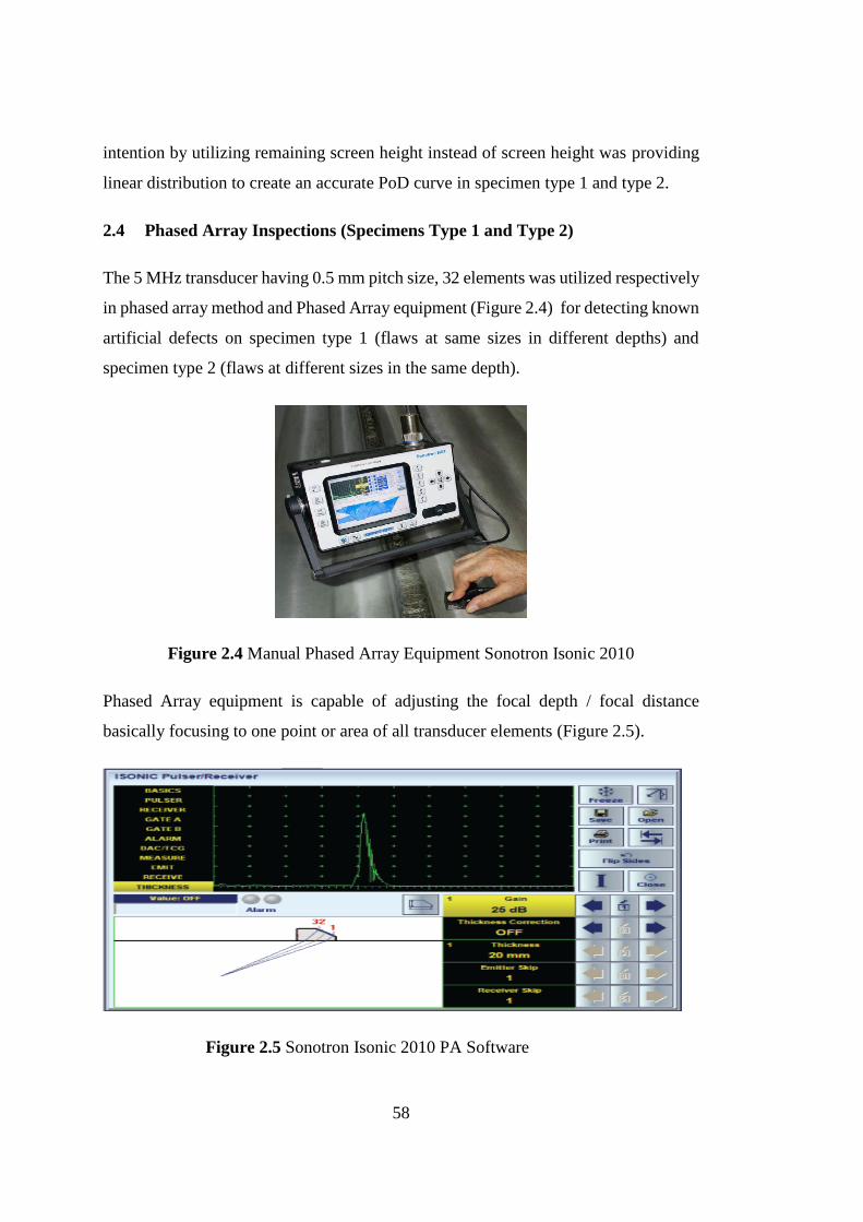
58

intention by utilizing remaining screen height instead of screen height was providing

linear distribution to create an accurate PoD curve in specimen type 1 and type 2.

2.4 Phased Array Inspections (Specimens Type 1 and Type 2)

The 5 MHz transducer having 0.5 mm pitch size, 32 elements was utilized respectively

in phased array method and Phased Array equipment (Figure 2.4) for detecting known

artificial defects on specimen type 1 (flaws at same sizes in different depths) and

specimen type 2 (flaws at different sizes in the same depth).

Figure 2.4 Manual Phased Array Equipment Sonotron Isonic 2010

Phased Array equipment is capable of adjusting the focal depth / focal distance

basically focusing to one point or area of all transducer elements (Figure 2.5).

Figure 2.5 Sonotron Isonic 2010 PA Software

59

2.5 Ultrasonic inspections (Specimen Type 3 – The Butt Welded Plate)

Figure 2.6 Calculation of sound path distance

According to probe refraction angle (70°) and plate thickness (10 mm), half sound

path, full sound path and 3/2 sound path were calculated (Figure 2.6 and Table 2.3).

10

cos 70 = 29,23 mm (Sp / 2), Sp = 58,46 mm, 3/2 Sp = 87,69 mm

According to calculations,

3040

3250=

sin 𝛼

sin 70 , the angle of refraction (α) was found as 61.5°. If this angle applied to

equation of 10

cos 61= 20,6 value obtained. But in the device display the measured value

approximately was seen as “19 “due to sound attenuation and angle change. When the

calculated value and measured value deviation is considered, the real sound velocity

was found as 3134 m /s.

Table 2.3 Sp Calculations

Sound Path Skip Distance

Sp 20 19 3

2 Sp

30 28

2Sp 40 38

5

2 Sp 50 47

60

Finally, the angle was calculated;

tan−1 0,94 ≅ 43°

From the Snell’s law

sin 43

sin 45=

×

3250 , velocity = 3134 m /s

The calculation about sound pressure decrease was performed for the austenitic

stainless steel test blocks comparing with plain carbon steel K1 block as a reference.

The mean attenuation values were calculated by repeating the measurement three times

on each specimen. For the velocity and sound pressure drop measurements in the test

block, the time of flight between two back-wall echoes was measured using

Krautkrammer USM 35 device.

Firstly, 45 ° probe was used for calculations, on the K1 block the first peak is obtained

at 25 𝑚𝑚

sin 45= 35,35 𝑚𝑚 at 24.5 dB sound pressure, and second peak is 70.7 mm at 27

dB. Therefore, for 35 mm sound distance, sound pressure loss corresponds to 2.5 dB,

and it is approximately 70 dB / m.

Secondly, the attenuation calculations were performed by using half skip and full skip

method for the butt welded specimen by 45 ° probe (Figure 2.6), the first signal

obtained at 10 𝑚𝑚

sin 47 = 13,67 mm at 27 dB, while 1,5 Sp = 41,8 mm obtained at 31.3 dB.

Hence, 4.3 dB approximately sound pressure loss was occurred on the austenitic

stainless specimen for the 28 mm sound distance. Consequently, the attenuation rate

corresponds to 1.54 dB / cm for the transition from weld metal. On the other hand, in

case of the same measurements were performed on the parent metal of butt welded

specimen, the attenuation rate corresponds to 1.06 and 1.22 dB / cm at 45 ° and 60 °

test angles respectively.

In the last part, 70° - 4 MHz probe was used for the UT inspection of austenitic

stainless steel plate and 3140

3250=

sin 𝛼

sin 70 so that α = 65° is found and then sound distance

calculation plate thickness 10 𝑚𝑚

cos 65= 23.6 𝑚𝑚, while the sound distances are Sp = 47.2

61

mm and 3

2 Sp = 70.9 mm as well. When the sound distance is 23.7 mm, the sound

pressure loss is approximately equal to 4 dB which is equivalent to 168 dB / m.

Because of the sound pressure losses and attenuation, the signal amplitudes decrease

as the distance passed by sound beam increases. Sizing functions allow us to do

evaluate the size of a crack or discontinuity, DAC method was used to calculate sizing

functions (Figure 2.7). 2 mm diameter side drilled holes of specimen type 1 were used

for drawing a proper DAC curve.

Figure 2.7 DAC curve schematic presentation

Figure 2.8 Display of 2nd defect signal

62

2.6 Automated Phased Array Inspections with Encoder (Specimen Type 3 –

The Butt Welded Plate)

Automated PA inspections with Encoder were performed by Olympus Omniscan MX

Flaw Detector (Figure 2.8 and 2.9)

Figure 2.9 Phased Array testing apparatus – Olympus Omniscan MX

Second, probe configuration and position according to weld bevel were carried out

with ES Beam Tool3 software piece and weld configuration (Figure 2.14).

Figure 2.10 ES Beam Tool3 probe configuration

The probe configuration such as frequency, total elements used and particularly

position of probe, together with material properties like sound velocity, sectorial beam

63

set configuration were adjusted (Figure 2.10 – 2.11). The aperture elements, the

minimum and maximum angle were adapted to the Omniscan MX software by using

the ES Beam Tool3. The intention was to implement exactly the same configuration

parameters which are determined to apply them in real inspection. Moreover, the

encoder position on the x- axis of the welded plate is a significant factor in terms of

detection of flaws.

Figure 2.11 Sectorial beam set configuration

Finally, five tests including different parameters in focal depth and the x-axis / - x axis

of butt welded palte (specimen type 3) inspections were carried out. The software setup

and all parameters are demonstrated in Table 2.4.

64

Table 2.4 Phased array Omniscan MX software parameters

Probe Characterization

Probe Model Probe Serial #

5L16-A10 G1255

Probe Frequency Peak Frequency Wedge Model Wedge Angle Probe Aperture

5.00 MHz N/A SA10-N55S 5L16-

A10 36.1º 9.60 mm

Lower Frequency Higher Frequency Center Frequency Bandwidth (MHz) Bandwidth (%)

-6 dB N/A N/A N/A N/A N/A

-20 dB N/A N/A N/A N/A N/A

Date Time Procedure Calibration Block Characterization

Gain A%

N/A N/A N/A N/A N/A N/A

Setup

A:45.0 Sk:090 L:001

Beam Delay Start (Half Path) Range (Half Path) Max. PRF Type Averaging Factor

10.95 us -0.25 mm 180.71 mm 5 PA 1

Scale Type Scale Factor Video Filter Pretrig. Rectification Band-Pass Filter

Compression 36 Off 0.00 µs FW None (0.54 - 22

MHz)

Voltage Gain Mode Wave Type Sound Velocity Pulse Width

40 (Low) 11.10 dB PE (Pulse-Echo) User-Defined 3137.4 m/s 100.00 ns

Scan Offset Index Offset Skew

0.00 mm 0.00 mm 90.0º

Gate Start Width Threshold Synchro

I 110.48 mm 3.65 mm 20.00 % Pulse

A 0.49 mm 3.92 mm 17.00 % Pulse

B 73.61 mm 3.65 mm 30.00 % Pulse

TCG Point

Number Position (Half-Path) Gain

1 0.00 mm 0.0 dB

65

According to 1st, 2nd and 3rd inspection, repeated detections are marked with the same color in

Table 2.5.

2 1.66 mm 9.9 dB

3 7.71 mm 8.2 dB

4 13.62 mm 5.8 dB

Calculator

Used Element

Qty. First Element Last Element Resolution Wave Type Material Velocity

16 1 16 1.0 User-Defined 3137.4 m/s

Start Angle Stop Angle Angle Resolution Focal Depth Law

Configuration

45.0º 70.0º 1.0º 10.00 mm Sectorial

Part

Material Geometry Thickness

STEEL, STNLSS Plate 10.00 mm

Scan Area

Scan Start Scan Length Scan Resolution Index Start Index Length Index Resolution

0.00 mm 300.00 mm 12.00 mm 0.00 mm 0.00 mm 1.00 mm

Synchro Max. Scan

Speed

Encoder 60.00 mm/s

Axis Encoder Encoder Type Encoder Resolution Polarity

Scan 1 Quadrature 12.07 step/mm Normal

Index Off Off Off Off

66

Table 2.5 Results of the first trial (10 mm focal depth)

1st Inspection

Entry # Scan

(mm)

Index

(mm) Group Channel A% (%)

DA^

(mm)

PA^

(mm)

SA^

(mm) A% (%)

DA^

(mm)

ViA^

(mm)

VsA^

(mm)

1 * 12.00 0.50 1 53.0º 73.2 6.06 8.98 23.16 73.2 6.06 8.98 12.00

2 * 0.00 0.50 1 51.0º 77.1 5.65 7.90 22.80 77.1 5.65 7.90 0.00

3 * 300.00 0.50 1 55.0º 2.4 --- --- --- 2.4 --- --- ---

4 * 180.00 0.50 1 70.0º 27.8 8.62 16.53 25.19 27.8 8.62 16.53 180.00

2nd Inspection

Entry # Scan

(mm)

Index

(mm) Group Channel A% (%)

DA^

(mm)

PA^

(mm)

SA^

(mm) A% (%)

DA^

(mm)

ViA^

(mm)

VsA^

(mm)

1 * 12.00 0.50 1 53.0º 73.2 6.06 8.98 23.16 73.2 6.06 8.98 12.00

2 * 0.00 0.50 1 51.0º 77.1 5.65 7.90 22.80 77.1 5.65 7.90 0.00

3 * 300.00 0.50 1 55.0º 2.4 --- --- --- 2.4 --- --- ---

4 * 180.00 0.50 1 70.0º 27.8 8.62 16.53 25.19 27.8 8.62 16.53 180.00

5 * 48.00 0.50 1 67.0º 34.4 7.45 22.03 32.11 34.4 7.45 22.03 48.00

6 * 0.00 0.50 1 57.0º 25.1 7.27 10.67 23.37 25.1 7.27 10.67 0.00

3rd Inspection

Entry # Scan

(mm)

Index

(mm) Group Channel A% (%)

DA^

(mm)

PA^

(mm)

SA^

(mm) A% (%)

DA^

(mm)

ViA^

(mm)

VsA^

(mm)

1 * 96.00 0.50 1 69.0º 30.9 6.29 9.12 17.55 30.9 6.29 9.12 96.00

2 * 72.00 0.50 1 70.0º 29.0 9.12 17.91 26.66 29.0 9.12 17.91 72.00

3 * 36.00 0.50 1 64.0º 27.8 8.51 15.63 26.21 27.8 8.51 15.63 36.00

4 * 48.00 0.50 1 69.0º 23.1 6.45 9.54 18.01 23.1 6.45 9.54 48.00

5 * 60.00 0.50 1 70.0º 29.0 9.16 22.64 31.70 29.0 9.16 22.64 60.00

6 * 48.00 0.50 1 70.0º 30.5 6.80 11.53 19.87 30.5 6.80 11.53 48.00

7 * 24.00 0.50 1 70.0º 32.9 2.48 -0.34 7.24 32.9 2.48 -0.34 24.00

8 * 24.00 0.50 1 68.0º 48.1 8.30 21.58 31.25 48.1 8.30 21.58 24.00

9 * 36.00 0.50 1 70.0º 29.4 9.18 22.57 31.62 29.4 9.18 22.57 36.00

10 * 84.00 0.50 1 70.0º 27.0 8.93 23.26 32.36 27.0 8.93 23.26 84.00

11 * 24.00 0.50 1 70.0º 44.6 8.71 23.87 33.00 44.6 8.71 23.87 24.00

67

Since the probe characteristics, material properties and the setup or calibration

parameters were not changed, there was no need to display repetition tables. In the

second trial, the focal depth was adjusted on 25 mm, the material velocity was changed

to 3146.1 m/s, and angle resolution was set to 0.5° instead of 1° in the calculator (Table

2.6). A crucial point of inspection, the probe start and stop angles were set or expanded

from 45° to 55° and 70° to 75° with respect to position of the encoder.

Table 2.6 Phased array Omniscan MX software parameters for the Second trial

Calculator

Used Element

Qty. First Element Last Element Resolution Wave Type

Material

Velocity

16 1 16 1.0 User-Defined 3146.1 m/s

Start Angle Stop Angle Angle

Resolution Focal Depth

Law

Configuration

55.0º 75.0º 0.5º 25.00 mm Sectorial

Setup

A:55.0 Sk:090 L:001

Beam Delay Start (Half Path)

Range (Half Path)

Max. PRF Type

11.55 us -2.01 mm 176.18 mm 5 PA

Scale Type Scale Factor Video Filter Pretrig. Rectification

Compression 35 Off 0.00 µs FW

Voltage Gain Mode Wave Type Sound Velocity

40 (Low) 9.60 dB PE (Pulse-Echo)

User-Defined 3146.1 m/s

Scan Offset Index Offset Skew

0.00 mm 0.00 mm 90.0º

68

Table 2.7 Results of the second trial no (25 mm focal depth)

1st Inspection

Entry # Scan

(mm)

Index

(mm) Group Channel

A%

(%)

DA^

(mm)

PA^

(mm)

SA^

(mm)

A%

(%)

DA^

(mm)

ViA^

(mm)

VsA^

(mm)

1 * 0.00 0.50 1 62.5º 55.2 7.22 16.41 27.67 55.2 7.22 16.41 0.00

2 * 144.00 0.50 1 57.5º 32.5 6.59 12.19 24.95 32.5 6.59 12.19 144.00

3 * 216.00 0.50 1 75.0º 28.6 7.04 94.32 104.47 28.6 7.04 94.32 216.00

4 * 180.00 0.50 1 75.0º 43.4 7.28 95.20 105.38 43.4 7.28 95.20 180.00

5 * 252.00 0.50 1 75.0º 41.1 7.27 95.17 105.35 41.1 7.27 95.17 252.00

6 * 96.00 0.50 1 75.0º 30.9 6.65 92.86 102.96 30.9 6.65 92.86 96.00

2nd Inspection

Entry # Scan

(mm)

Index

(mm) Group Channel

A%

(%)

DA^

(mm)

PA^

(mm)

SA^

(mm)

A%

(%)

DA^

(mm)

ViA^

(mm)

VsA^

(mm)

1 * 84.00 0.50 1 57.0º 54.4 6.23 12.28 25.28 54.4 6.23 12.28 84.00

2 * 204.00 0.50 1 75.0º 66.5 7.09 94.52 104.68 66.5 7.09 94.52 204.00

3 * 48.00 0.50 1 64.5º 57.5 6.96 19.49 30.30 57.5 6.96 19.49 48.00

4 * 24.00 0.50 1 64.5º 68.1 7.54 18.27 28.95 68.1 7.54 18.27 24.00

5 * 84.00 0.50 1 64.5º 52.8 6.91 19.59 30.41 52.8 6.91 19.59 84.00

6 * 252.00 0.50 1 75.0º 49.7 7.84 97.32 107.57 49.7 7.84 97.32 252.00

7 * 72.00 0.50 1 70.0º 28.6 3.83 3.37 11.19 28.6 3.83 3.37 72.00

8 * 24.00 0.50 1 63.5º 58.3 7.92 16.24 27.08 58.3 7.92 16.24 24.00

9 * 252.00 0.50 1 75.0º 45.0 6.30 91.56 101.61 45.0 6.30 91.56 252.00

10 * 72.00 0.50 1 70.5º 29.4 4.33 5.15 12.98 29.4 4.33 5.15 72.00

11 * 96.00 0.50 1 75.0º 42.7 6.73 93.18 103.29 42.7 6.73 93.18 96.00

12 * 240.00 0.50 1 75.0º 34.0 6.40 91.95 102.02 34.0 6.40 91.95 240.00

69

2.7 Manual Phased Array Inspection on Butt Welded Plate (Specimen Type 3)

In the manual inspections with Phased Array system, the probe is scanned towards and

away from the weld line, and the operator follows the screen for any signal detection.

Phased Array provides much simpler detection along with S-scan, C-Scan or B-Scan

displays rather than simple A-Scan [27].

Figure 2.12 Weld bevel image on the screen of Sonotron Isonic 2010

Manual Phased Array inspection was carried out by Sonotron isonic 2010 device and

linear array probe with 32 elements (Figure 2.12 – 2.13). Since the inspection is time

based data collection, i.e., depends on operator’s speed, the position and length of

defects are influenced by manually time-based scanning or beam sweeping. Therefore,

these results are not acceptable in terms of probability of detection analysis because

there is no relationship between defect size and defect amplitude or signal and or any

other verification codes such as ASME Code Case 2235.

Nevertheless, Manual Phased Array inspections were performed on butt welded plate

in order to prove the dominance of Phased Array over the conventional UT from the

point of detecting discontinuities.

70

The advantages such as beam steering and

sweeping, and adjusting focus distance, give a superiority to Phased Array over

conventional ultrasonic testing in terms of detection capabilities.

Figure 2.14 Defect list captured by Sonotron Isonic 2010

Data demonstrated in Figure 2.14 are inaccurate since the defect sizes are not matching

with defect amplitudes due to time based scanning errors. Time-based scanning can be

used only to demonstrate detection of a flaw, it does not give properly defect positions

or size results.

Figure 2.13 Manual Phased Array inspection

71

2.8 Probability of Detection Analysis

The inspection results are transferred to probability of detection analysis software

program (mh1823) and then, the rules and procedure steps in the MIL-HDBK-1823A

criteria were followed for drawing the Probability of Detection graphs (PoD).

In order to evaluate the reliability of a nondestructive method, there are two realistic

and probabilistic approach. Namely, the first one “hit/miss” data is based on whether

a flaw detected or not. The second one is used for defect sizes versus signal responses

where this approach is appropriate for eddy current or ultrasonic testing methods due

to outputs of these methods. Selected feedback about flaw property for ultrasonic and

eddy current case is called â data (i.e. “a hit / miss data”) or “signal response” data

[18].

PoD curves were generated with data obtained from artificial defect sizes versus signal

responses on the behalf of conventional ultrasonic and Phased array inspections. In

case of manual Phased array inspection on the butt welded plates since the real defect

sizes are unknown and time based inspection performed without encoder, the data

derived from this type of inspection is not appropriate for generating PoD curves.

All PoD curves were created with the correlation of “a vs â” data. The results of

inspections were processed by using mh1823 software [26].

72

73

CHAPTER 3

RESULTS and DISCUSSION

3.1 Microstructure

The representative micrographs for the specimen type 3 are given in Figure 3.1. The

number of intercepts is 408 and the mean intercept length values for the parent metal

were found to be 13 µm, which corresponds to ASTM Grain Size Number G: 9. 24

according to ASTM E 1382. On the other hand, in the heat affected zone the number

of intercepts is 436 and the mean intercept length values were found to be 12 µm.

(a) (b)

Figure 3.1 Representative micrographs for the specimen type 3 Parent, HAZ and weld

metal at (5 x) (a), Fusion line at (20 x) (b)

The average grain size of the parent metal is 13 µm while it is approximately 12 µm

in the heat affected zone. These results indicate occurrence of recrystallization in the

74

heat affected zone. Figure 3.2 shows the mean micro hardness values of the parent

metal, heat affected zone and weld metal.

Figure 3.2 Micro hardness values versus distance to weld line

Grain size and micro hardness values are in accordance with literature [25, 32]. An

example is given in Table 3.1.

Table 3.1 Grain sizes and mechanical values of the AISI 304 [25]

The only difference between literature data and the results of this study is high

hardness of the weld metal. The reason is the selection of the filler material (Table 2.2)

intentionally wrong to create inherent discontinuities since the whole study is based

on probability of detection of such defects.

75

It was assumed that the differences in the grain morphology of the cast austenitic

stainless steels (equiaxed or columnar) can be detected by longitudinal waves. The

estimate is based on the attenuation of equiaxed structure more than attenuation of

columnar structure in the study of P. Ramuhalli et al. [28]. While the bandwidth

frequency of transducers is being lowered, the difference in attenuation is getting

smaller (300 to 800 kHz). It has been already reported that attenuation in columnar

grain structure is less than ~ 2 dB/cm, while it is greater than or equal to ~2.5 dB/cm

in the equiaxed-grain structure (Table 3.2). Since the beam skew, texture and related

degree of anisotropy, also preferred orientations of grains were not involved, it seems

that the attenuation in columnar grain structure is less than that in equiaxed structure.

Moreover, lower frequencies (longer wavelengths) scattering from the grain

boundaries (whether equiaxed or columnar) is low particularly for small ultrasonic

path lengths (corresponding to the first back-wall signal). As the sound path distance

escalates (corresponding to second, third, and later reflections), scattering from the

more grain boundaries in equiaxed structures becomes more significant and results in

larger attenuation values.

Table 3.2 Average attenuation in the columnar and equiaxed structure [28]

In general ultrasonic inspection is very hard due to inhomogeneous media in the coarse

columnar grains, it is likely difficult to predict ultrasonic capabilities, or to choose

reference for the UT inspection. On the other hand, in case of fine structures (equiaxed

microstructure) it is more homogeneous acting like transverse isotropic. However,

attenuation or background noise can be an issue as important as in coarse columnar

grain structures. Therefore, the presence of fine columnar zone does not interfere the

detection and the localization of defects. Since a stable echo is preferred to disturbed

one, these materials are considered easier to control [38].

76

Figure 3.3 Representative axial-radial cross sections of the specimen type 3

Based on the calculations carried out by different frequencies and angles, the mean

attenuation values are given in Table 3.3 for different test frequencies by longitudinal

waves, and in Table 3.4 for different test angles by shear waves.

Table 3.3 The mean attenuation values in the specimen type 1 and 2 (longitudinal

wave)

Test frequency Longitudinal Wave

4 MHz 2 MHz 1 MHz

Sound velocity (m /s) 5752 5766 5617

Mean attenuation (dB / cm) 0.56 0.58 0.78

Attenuation rate in equiaxed structure which was measured by using half skip and full

skip method is higher than that in the columnar structure of specimen type 3 butt

welded plate (Table 3.4).

77

Table 3.4 The mean attenuation values in the columnar and equiaxed structure of the

specimen type 3 butt welded plate (shear wave)

Angles of Test Probes

45° 60 ° 45° 60 °

Columnar Equiaxed

Sound velocity (m /s) 3106 3137 3140 3135

Mean Attenuation (dB / cm) 1.06 1.22 1.54 1.50

Ultrasonic propagation is homogeneous close to fusion line because of the equiaxed

microstructure (relatively finer grains) of heat affected zone. Although the sound

propagation in the columnar structure of austenitic test blocks is commonly harder than

that in equiaxed microstructure, attenuation in fine grains can, however, be as

significant as in coarse columnar grain structures regarding the chemical composition

or the manufacturing conditions of the specimen. The difference in attenuation rate

measurement might have arisen because the weld material was chosen intentionally

inappropriate for the welding in order to create defects as much as possible.

Furthermore, the percentage of ferrite have direct impact on ultrasonic attenuation.

According to the study of Ferreira et al. [37], the increase in the percentage of ferrite

in the microstructure, resulted in the decrease of the sonic speed, and in sonic

attenuation increase. Also, the higher percentages of ferrite (Figure 3.2) lead to the

highest average hardness values at AISI 304L of the butt welded plate specimen type

3.

3.2 Results of Ultrasonic and Phased Array Inspections

Table 3.5, 3.7 shows the data retrieved from the flaws at different depths (Specimen

Type 1), while Table 3.6, 3.8 shows the data retrieved from the flaws at different sizes

at the same depth (Specimen Type 2) by ultrasonic method and Phased Array testing

respectively. In addition, Table 3.9 demonstrates the data collected from the flaws in

butt welded plate (specimen type 3) by conventional ultrasonic inspection.

78

Table 3.5 UT data retrieved from the flaws at different depths of (Specimen Type 1)

ID Sound path

(mm) Remaining screen

height (%) ID Sound path (mm)

Remaining screen height (%)

1 10,71 1 1 10,49 1

2 22,46 34 2 22,38 44,44

3 34,47 59 3 34,28 62

4 47,1 67 4 46,29 72,6

5 58,52 75 5 58,27 79,6

6 71,16 77 6 70,85 83

7 83,2 81 7 82,2 87,1

8 95,32 83 8 94,24 88,6

9 107,3 85 9 106,13 89

10 119,3 87 10 118,29 93

ID Sound path

(mm) Remaining screen

height (%) ID Sound path (mm)

Remaining screen height (%)

1 10,06 1 1 10,34 1

2 22,57 34 2 22,4 46

3 34,89 59 3 34,6 61

4 47,0 67 4 45,7 72

5 58,3 73 5 58,6 78,8

6 70,9 76 6 70,9 82

7 83,4 81 7 82,6 86,9

8 95,22 83 8 94,2 89,3

9 107,1 86 9 106,6 89,4

10 118,8 88 10 118,4 92,5

Table 3.6 UT data retrieved from the flaws at different sizes at the same depth

(Specimen Type 2)

ID Screen

height (%) Amplitude

(dB) ID

Screen height (%)

Amplitude (dB)

5 mm 99 21,9 5 mm 99 18,8

4,5 mm 97,5 21,9 4,5 mm 94,7 18,8

4 mm 93,2 21,9 4 mm 88,1 18,8

3,5 mm 84,9 21,9 3,5 mm 82,2 18,8

3 mm 80,2 21,9 3 mm 79,5 18,8

2,5 mm 74,8 21,9 2,5 mm 74,4 18,8

2 mm 69,3 21,9 2 mm 65,4 18,8

1,5 mm 61,5 21,9 1,5 mm 54,8 18,8

1 mm 54,8 21,9 1 mm 48,1 18,8

0,8 mm 48,5 21,9 0,8 mm 35,8 18,8

0,5 mm 41,5 21,9 0,5 mm 41,1 18,8

79

ID Screen

height (%) Amplitude

(dB) ID

Screen height (%)

Amplitude (dB)

5 mm 99 20,5 5 mm 99 19,2

4,5 mm 98,1 20,5 4,5 mm 95,3 19,2

4 mm 93,5 20,5 4 mm 89,2 19,2

3,5 mm 85 20,5 3,5 mm 84,2 19,2

3 mm 80,6 20,5 3 mm 79,6 19,2

2,5 mm 74,9 20,5 2,5 mm 74,9 19,2

2 mm 69,1 20,5 2 mm 65,6 19,2

1,5 mm 61,9 20,5 1,5 mm 54,9 19,2

1 mm 55,2 20,5 1 mm 48,3 19,2

0,8 mm 48,7 20,5 0,8 mm 35,4 19,2

0,5 mm 41,2 20,5 0,5 mm 41,0 19,2

Table 3.7 PA data retrieved from the flaws at different depths (specimen Type 1)

ID Sound Path Remaining

Screen Height

ID Sound Path

Remaining Screen Height

1 11,1 1 1 10,8 0,5

2 22,28 39 2 20,32 35,6

3 36,2 52 3 35,1 52,3

4 46,59 62,6 4 48,53 60,9

5 57,23 69,7 5 56,39 69,9

6 65,75 77 6 67,6 77,8

7 81,1 84,1 7 80,9 83,5

8 93,34 87,6 8 94,1 88

9 104,11 88,6 9 106 89,9

10 117,19 92,5 10 119,2 92,6

ID Sound Path Remaining

Screen Height

ID Sound Path

Remaining Screen Height

1 13 1 1 11,5 0,8

2 23,3 36,2 2 21 36,8

3 36,1 52,9 3 36,1 53,8

4 45,8 58,6 4 49,2 61,5

5 58 70 5 57,5 69,9

6 66,1 77,6 6 66,4 78

7 82,2 82,8 7 82 84,5

8 94,5 88 8 95,2 88

9 105,1 89,5 9 107,2 89,9

10 118,2 92,3 10 117,7 92,6

80

Table 3.8 PA data retrieved from the flaws at different sizes at the same depth

(Specimen Type 2)

ID Flaw Size(mm) Screen Height

ID Flaw

Size(mm) Screen Height

1 5 99 1 5 99

2 4,5 97,5 2 4,5 94,7

3 4 93,2 3 4 88,1

4 3,5 84,9 4 3,5 82,2

5 3 80,2 5 3 79,5

6 2,5 74,8 6 2,5 74,4

7 2 69,3 7 2 65,4

8 1,5 61,5 8 1,5 54,8

9 1 54,8 9 1 48,1

10 0,8 48,5 10 0,8 35,8

11 0,5 41,5 11 0,5 41,1

Focal depth 41,8 Focal Depth 38,3

ID Flaw Size(mm) Screen Height

ID Flaw

Size(mm) Screen Height

1 5 98 1 5 99,5

2 4,5 97,2 2 4,5 95,5

3 4 93 3 4 89,2

4 3,5 85,3 4 3,5 84,7

5 3 81,7 5 3 81,2

6 2,5 74,4 6 2,5 76,2

7 2 70,1 7 2 67,3

8 1,5 62,6 8 1,5 55,5

9 1 56 9 1 49,9

10 0,8 47 10 0,8 37,1

11 0,5 42,3 11 0,5 36,6

Focal depth 41,8 mm Focal Depth 38,3 mm

Table 3.9 Conventional ultrasonic inspection on butt welded specimen type 3

Defect No Sp Ha (dB) A’ L (mm) Da

1 35,4 1,4 22 mm 43 5,3

2 38,45 4,2 26 mm 82 3,32

3 39,34 0,12 25 mm 140 3,36

4 37,66 2,2 23 mm 160 4,1

5 85,57 1,2 65 mm 194 3,8

6 35,10 2,0 19 mm 249 5

81

3.3 Probability of Detection (PoD) Analysis

All data retrieved from the inspection records determine the best model for the PoD

analysis, model which represents the data as a straight line and approximate constant

variance were selected for further analysis.

According to MIL-HDBK-1823A, the best model for assessing the data in terms of

PoD is to use log(X) and Cartesian(Y) since there is a linear relationship among the

collected data and constant slope.

Figure 3.3 Four possible a vs â models for Type 1 specimen (UT)

3.3.1 a vs â Linear Model for PoD Analysis of Type 1 Specimen (UT)

In linear model the x- axis is represented by logarithmic values and y- axis is

represented by Cartesian values, the bounding or censoring values have to be resolved.

All signal response data have two censoring, first one is left censor or background

noise and the second one is right censor corresponding to maximum amplitude value

obtained from inspection. Since the left and right censors are the significant factors

whether a data is beneficial or useless, a special attention or measure must be taken

while determining the boundaries.

82

Inspection threshold (âth) and decision threshold (âdec) are indispensable which have a

direct impact on PoD curves. The inspection threshold is the smallest value of â

recorded by the system, â is the decision threshold any signal above it is interpreted as

a hit, and below it as a miss. â value has a direct relationship with 50 % PoD. Decision

threshold is always greater than or equal to inspection threshold [29].

Figure 3.4 a vs â linear models for specimen type 1 (UT)

For PoD determination of the specimen type 1, sound path versus signal amplitude

evaluation data were recorded and transferred to mh1823 statistical program. In order

to generate PoD curve, the left censor is fixed on “1” and right censor is adjusted on

“100” for all cases. â decision is the crucial point in the POD analysis of signal response

data. The noise level detection for decision threshold can be admitted any value above

the noise level. However, determination of decision threshold affects the detectability

of the smallest defect size and false-positive detections (Figure 3.4).

83

Figure 3.5 a vs â parameter values in UT [26]

The flaw size versus signal response parameters were used for PoD curves and

analysis. The decision threshold influences directly on accuracy of testing. Also, four

fundamental criteria; linearity of the parameters, uniform variance, uncorrelated

responses and normal distribution of test flaw sizes have to be considered before

assessing any data [17].

To fulfill the conditions of PoD status, the decision threshold (â decision) was

determined as 40 (Figure 3.5).

3.3.2 a vs â Linear Model for PoD Analysis of Specimen Type 1 (PA)

In order to acquire linear model determination of data collected by Phased Array

inspections, the decision threshold (â decision) was determined as 25 since the PA

transducers having ability of focus depth adaptation and its near field zone is less than

that of conventional ultrasonic transducers (Figure 3.6).

84

Figure 3.6 a vs â linear model Specimen Type 1 (PA)

3.3.3 PoD Analysis of Specimen Type 1

PoD curve of specimen type 1 data derived from artificial flaw depth (a) versus signal

response (â) for ultrasonic testing and Phased Array are exhibited in Figure 3.7 and 3.8

respectively. In case for ultrasonic testing the 50 % PoD of flaw (a50) is 25.54 mm in

depth. In addition, 90 % PoD of flaw (a90) is 32.33 mm in depth and 90 % PoD of flaw

with a confidence interval of 95 % of a flaw (a90/95) depth is 35.05 mm from surface

were obtained.

85

Figure 3.7 PoD curve of specimen type 1 (UT)

Figure 3.8 PoD curve of specimen type 1 (PA)

86

Moreover, in case of Phased Array system, the 50 % PoD of flaw (a50) is 18.75 mm in

depth and 90 % PoD of flaw (a90) is 21.31 mm in depth. Finally, 90 % PoD of flaw

with a confidence interval of 95 % of a flaw (a90/95) depth is 22.35 mm.

According to results derived from PoD graphs, Phased Array testing gives better

results than conventional ultrasonic testing since near field zone is a setback for

conventional ultrasonic while the focus depth adaptation is an advantage for Phased

Array. Furthermore, depth of first flaw is 5 mm which was detected by PA while

conventional ultrasonic testing was not able to detect it due to near field zone effect.

3.3.4 PoD Analysis of Specimen Type 2

PoD curves for specimen type 2 given in Figure 3.09 and 3.10 show that the reliability

of the Phased Array system for determining the flaw size is slightly better than that of

the ultrasonic system.

Flaw sizes are representing 50 % PoD (a50) values for 1.028 mm in the ultrasonic

testing and 1.009 mm for the Phased array system. Projection of 90 % PoD of flaw

size (a90), 1.177 mm and 1.138 mm are determined for UT and PA respectively. Lastly,

90 % PoD with a confidence interval of 95 % of a flaw (a90/95) sizes are 1.236 mm in

the ultrasonic system and 1.19 mm in the Phased array system.

According to these results Phased Array inspection’s advantage over the conventional

ultrasonic is diminished for the specimen type 2. Since the distance of all flaw depths

are same (40 mm), there is no near field zone for UT and PA. Consequently, it must

be mentioned that the generated PoD curves highly depend on the data involved in

calculations. The significant factor is the decision threshold which is determined by

noise level for the material and linearity in terms of probability detection curving rules.

87

Figure 3.9 PoD curve for Type 2 specimen (UT)

Figure 3.10 PoD curve for Type 2 specimen (PA)

88

Table 3.10 Reliability values of flaw sizes and depths for ultrasonic (UT), phased

array (PA) systems

Reliability

Specimen Type 1

Specimen Type 2

UT PA UT PA

50 % PoD 25.54 mm 18.75 mm 1.028 mm 1.009 mm 90 % PoD 32.33 mm 21.31 mm 1.177 mm 1.138 mm

90 % PoD with a confidence interval of 95 %

35.05 mm 22.5 mm 1.236 mm 1.19 mm

The reliability of system depends on acceptance level, in other words selection of

decision threshold and in these cases, repeatability of the results by different operators.

Beside human factor, some other variables exist (Table 3.11).

Table 3.11 the Essential Variables in Ultrasonic and Phased Array Testing [19]

Flaw size / flaw orientation / flaw surface texture

Beam characteristics

The Flaw position according to sound path

Potential that the flaw was off-axis

Anisotropic characteristics of the materials tested

Coupling variation due to test surface texture

Texture of the local surface conditions where a skip is required

Weld cap and weld root geometry

Mismatch conditions, etc.

89

3.4 Evaluation of Manual Phased Array inspections

In ideal situation, the butt welded plate should have artificial defects representing

common discontinuities such as;

1. Smooth planar, to represent lack of side wall fusion.

2. Rough planar, to represent cracks.

3. Volumetric, to represent porosity or slag.

However, due to machining problems only volumetric bottom holes and one slot along

the weld line were created (Figure 3.11).

Figure 3.11 The holes and slot on the specimen type 3

During manual Phased Array inspections, by 5 MHz, 0.5 mm pitch size and 32

elements, the first angle 30° and last angle 70° of transducer, along with the delay line

wedge were used. The results derived from time based inspections are demonstrated

in Figure 3.12 - 3.13 subsequently.

90

Figure 3.12 the Detected flaws list and schematic display of flaws-1 (MPA)

Figure 3.13 The Detected flaws list and schematic display of flaws-2 (MPA)

91

Both inspection trials were performed without encoder so that the positions of defects

are not accurate but meandering scan of the weld and swiveling of the probe give some

opportunities regarding detection of flaws (Figure 3.14). It is observed that manual

Phased array inspections find out the bottom holes the position at 95 mm, 160 mm and

slot from 205 mm to 240 mm together with some other unknown natural weld flaws.

Figure 3.14 Meandering scan of the weld and swiveling of the probe [2]

Meandering and swiveling of the probe similar to conventional ultrasonic testing,

increase the chance of flaw detection since the PA system has more capabilities like

focal depth, sectorial scan and 32 number of elements firing instead of single element

transducer in ultrasonic testing. The bottom line is that Manual Phased Array detected

existing artificial holes and slot along with a lack of fusion which is a prevailing

discontinuity for butt welded plate in case of both side welding. Although lack of

fusion is not properly positioned by manual Phased Array system because of lack of

encoder, the flaw had been detected successfully yet (Figure 3.15).

Figure 3.15 The lack of fusion on manual PA display and destructive macro test

92

3.5 Evaluation of Automated Phased Array Inspections

Automated Phased Array inspections were carried out three times for 10 mm focal

depth, and two times for 25 mm focal depth. After removing the repeated detections

the final defect list were prepared for one line scan with encoder type Olympus ENC

1-2.5-DE as the Table 3.12 and 3.13.

Table 3.12 Phased Array 1st Trial (10 mm focal depth)

1st Inspection Table

Entry # Scan

(mm)

Index

(mm) Group Channel A% (%)

DA^

(mm)

PA^

(mm)

SA^

(mm) A% (%)

DA^

(mm)

ViA^

(mm)

VsA^

(mm)

1 * 12.00 0.50 1 53.0º 73.2 6.06 8.98 23.16 73.2 6.06 8.98 12.00

2 * 0.00 0.50 1 51.0º 77.1 5.65 7.90 22.80 77.1 5.65 7.90 0.00

3 * 300.00 0.50 1 55.0º 2.4 --- --- --- 2.4 --- --- ---

4 * 180.00 0.50 1 70.0º 27.8 8.62 16.53 25.19 27.8 8.62 16.53 180.00

5 * 48.00 0.50 1 67.0º 34.4 7.45 22.03 32.11 34.4 7.45 22.03 48.00

6 * 0.00 0.50 1 57.0º 25.1 7.27 10.67 23.37 25.1 7.27 10.67 0.00

7 * 96.00 0.50 1 69.0º 30.9 6.29 9.12 17.55 30.9 6.29 9.12 96.00

8 * 72.00 0.50 1 70.0º 29.0 9.12 17.91 26.66 29.0 9.12 17.91 72.00

9 * 36.00 0.50 1 64.0º 27.8 8.51 15.63 26.21 27.8 8.51 15.63 36.00

10* 60.00 0.50 1 70.0º 29.0 9.16 22.64 31.70 29.0 9.16 22.64 60.00

11 * 24.00 0.50 1 70.0º 32.9 2.48 -0.34 7.24 32.9 2.48 -0.34 24.00

12 * 84.00 0.50 1 70.0º 27.0 8.93 23.26 32.36 27.0 8.93 23.26 84.00

93

Table 3.13 Phased Array 2nd Trial (25 mm focal depth)

1st Inspection

Entry

#

Scan

(mm)

Index

(mm) Group Channel A% (%)

DA^

(mm)

PA^

(mm)

SA^

(mm)

A%

(%)

DA^

(mm)

ViA^

(mm)

VsA^

(mm)

1 * 0.00 0.50 1 62.5º 55.2 7.22 16.41 27.67 55.2 7.22 16.41 0.00

2 * 144.00 0.50 1 57.5º 32.5 6.59 12.19 24.95 32.5 6.59 12.19 144.00

3 * 216.00 0.50 1 75.0º 28.6 7.04 94.32 104.47 28.6 7.04 94.32 216.00

4 * 180.00 0.50 1 75.0º 43.4 7.28 95.20 105.38 43.4 7.28 95.20 180.00

5 * 252.00 0.50 1 75.0º 41.1 7.27 95.17 105.35 41.1 7.27 95.17 252.00

6 * 96.00 0.50 1 75.0º 30.9 6.65 92.86 102.96 30.9 6.65 92.86 96.00

7 * 84.00 0.50 1 57.0º 54.4 6.23 12.28 25.28 54.4 6.23 12.28 84.00

8* 204.00 0.50 1 75.0º 66.5 7.09 94.52 104.68 66.5 7.09 94.52 204.00

9 * 48.00 0.50 1 64.5º 57.5 6.96 19.49 30.30 57.5 6.96 19.49 48.00

10* 72.00 0.50 1 70.0º 28.6 3.83 3.37 11.19 28.6 3.83 3.37 72.00

11* 24.00 0.50 1 63.5º 58.3 7.92 16.24 27.08 58.3 7.92 16.24 24.00

12 * 240.00 0.50 1 75.0º 34.0 6.40 91.95 102.02 34.0 6.40 91.95 240.00

The inspections with the focal depth of 10 mm and 25 mm showed the same detection

capability. In order to evaluate the results easily, the Table 3.12 and 3.13 are combined

in Table 3.14.

Table 3.12 and 3.13 were reconstructed according to scan positions for avoiding

repeated measures considering easy evaluation. There are fifteen individually defect

possibility based on the one line automated Phased array scan, one by one was

examined in S-scan (Table 3.14).

94

Table 3.14 The list of flaws detected by Phased Array method

Detected Flaws Combined Table

Entry

#

Scan

(mm)

Index

(mm)

Gro

up

Channe

l

A (%) DA^

(mm)

PA^

(mm)

SA^

(mm)

A%

(%)

DA^

(mm)

ViA^

(mm)

VsA^

(mm)

1 * 0.00 0.50 1 51.0º 77.1 5.65 7.90 22.80 77.1 5.65 7.90 0.00

2* 12.00 0.50 1 53.0º 73.2 6.06 8.98 23.16 73.2 6.06 8.98 12.00

3 * 24.00 0.50 1 70.0º 32.9 2.48 -0.34 7.24 32.9 2.48 -0.34 24.00

4 * 36.00 0.50 1 64.0º 27.8 8.51 15.63 26.21 27.8 8.51 15.63 36.00

5 * 48.00 0.50 1 67.0º 34.4 7.45 22.03 32.11 34.4 7.45 22.03 48.00

6* 60.00 0.50 1 70.0º 29.0 9.16 22.64 31.70 29.0 9.16 22.64 60.00

7* 72.00 0.50 1 70.0º 29.0 9.12 17.91 26.66 29.0 9.12 17.91 72.00

8 * 84.00 0.50 1 70.0º 27.0 8.93 23.26 32.36 27.0 8.93 23.26 84.00

9 * 96.00 0.50 1 69.0º 30.9 6.29 9.12 17.55 30.9 6.29 9.12 96.00

10* 144.00 0.50 1 57.5º 32.5 6.59 12.19 24.95 32.5 6.59 12.19 144.00

11 * 180.00 0.50 1 70.0º 27.8 8.62 16.53 25.19 27.8 8.62 16.53 180.00

12* 204.00 0.50 1 75.0º 66.5 7.09 94.52 104.68 66.5 7.09 94.52 204.00

13 * 216.00 0.50 1 75.0º 28.6 7.04 94.32 104.47 28.6 7.04 94.32 216.00

14 * 240.00 0.50 1 75.0º 34.0 6.40 91.95 102.02 34.0 6.40 91.95 240.00

15 * 252.00 0.50 1 75.0º 41.1 7.27 95.17 105.35 41.1 7.27 95.17 252.00

The first indication (Figure 3.16) is at the depth of 5.65 mm, it is more likely to be lack

of fusion or incomplete penetration since the position of flaw is near to beginning of

the root pass.

The second indication (Figure 3.17) is more likely to be subsequent of the flaw

beginning from starting point of the plate. It is well known that start – stop or finish

zones are prone to be created defects particularly in gas metal arc welding procedure

(GMAW), in this case it is approximately 20-25 mm. Flaw length of 3rd (Figure 3.18)

indication is approximately 25 mm at the depth of 2.48 mm.

95

Figure 3.16 Evaluation of 1st data

Figure 3.17 Evaluation of 2nd data

Figure 3.18 Evaluation of 3rd data

96

4th, 5th and 6th indications (Figure 3.19, 3.20, 3.21) resemble probably small defects

at the depth of 8.51, 7.45 and 9.16 mm respectively.

7th and 8th indications (Figure 3.22 and 3.23) are very close to bottom of the plate

since their depth starting point at 9.12 and 8.93 mm in the t=10 mm nominal thickness

of the plate.

Figure 3.19 Evaluation of 4th data

Figure 3.20 Evaluation of 5th data

97

Figure 3.21 Evaluation of 6th data

Figure 3.22 Evaluation of 7th data

Figure 3.23 Evaluation of 8th data

98

9th and 10th indications (Figure 3.24) correspond to the bottom holes that were

artificially created. 11th (Figure 3.25) indication possibly refers to a small defect at the

depth of 8.62 mm.

Figure 3.24 Evaluation of 9th and 10th data

Figure 3.25 Evaluation of 11th data

12th to 15th (Figure 3.26-3.27) indications more likely correspond to the slot artificially

created starting from 205 mm to ending at 245 mm. Since the slot was not created in

properly, signal amplitudes diverted.

99

Figure 3.26 Evaluation of 12th data

Figure 3.27 Evaluation of 13th, 14th and 15th data

To sum up, automated Phased Array system is successful to detect positions and sizes

of inherent weld discontinuities including artificially flaws. Although manual Phased

Array inspection has a slight advantage to detect discontinuities by meandering and

swiveling of the probe, it does not give a clue about defect position and size. Manual

Phased Array is still successful to detect lack of fusion in the side wall of root pass

which requires some angle. Automated Phased Array provides exact position and sizes

of incomplete root fusion along with lack of fusion in the side wall and moreover, it

succeeded to detect artificial flaws. Therefore, automated Phased Array has superiority

100

in terms of detecting discontinuities over the manual Phased Array and conventional

ultrasonic testing.

As for ultrasonic testing, detection success on artificial flaws test blocks (Specimen

Type 1 and Type 2) has insignificant difference compare to manual Phased Array in

the manner of PoD (Figure 3.09 – 3.10). On the other hand, conventional ultrasonic

testing is not successful for detection of flaws in butt welded plate (Specimen Type 3)

compare to Phased Array system. Since beam angles are refracted and speed of sound

is eligible for change due to anisotropic media, Phased Array is secure the inspection

with firing multiple elements, steering and focusing abilities rather than one single

transducer element of conventional ultrasonic testing. It can be deduced that ultrasonic

testing detection capability is less than Phased Array and artificial defect position is

deviated (Table 3.9).

3.6 The radioscopy testing of the butt welded plate (specimen type 3)

The results of automated and manual Phased Array inspections were compared with

radioscopic inspection (Figure 3.28) for verification purpose.

Figure 3.28 Radioscopic image of the specimen type 3 (200 kV)

101

Figure 3.29 Radiographic image of the specimen type 3 (200 kV)

As seen in the Figure 3.28, there is an incomplete fusion in the root of weld between

the reference point at 0 mm and lasting at 25-30 mm. The image proves that the lack

of fusion in the side wall was detected clearly. Meanwhile automated and manual

Phased Array inspections also detect the incomplete fusion in the root pass and lack of

fusion in the side wall of the root pass.

While the real time radioscopy was able to detect volumetric incomplete and lack of

fusion, it does not provide certain sizes of these discontinuities. On the other hand,

indications of other flaws detected by automated Phased Array were not able to detect

by real time radioscopy.

3.7 The macroscopic inspection of the butt welded plate (specimen type 3)

Prior to macroscopic examination the surface of the specimen was etched with

specimen 60:40 ratio −70 wt. % HNO3 H2O, 10 mA / cm2 for 4-5 seconds. Incomplete

fusion in the root pass and lack of fusion in the side wall of the root pass are clearly

seen in Figure 3.29.

Figure 3.30 The macroscopic image of the specimen type 3

102

103

CHAPTER 4

CONCLUSION

The main objective of this thesis is to investigate and compare the abilities of manual

and automated Phased array systems with conventional ultrasonic test system for

detection of the flaws in austenitic stainless steel blocks and welds.

The results were compared with the probability of detection (PoD) concept. Three

types of test blocks were prepared from AISI Type 304 steel. First specimen is the

block having 2 mm ø side drilled holes created at different depths from 5 mm to 113

mm; second specimen has various side drilled holes with diameters between 0.5 mm

to 5 mm created at the 40 mm depth; third specimen is the GMAW welded 10 mm

thick plate having artificial and natural defects.

Initially, conventional ultrasonic testing was compared with manual Phased Array

(PA) system for detecting the artificially created flaws. Next, the manual PA system

(time based inspection) was compared with the automated PA system (encoder based

inspection) for detection of the artificially created defects (bottom holes and slot) in a

block and natural discontinuities in the welded plate. Grain size, micro hardness,

attenuation rate measurements, radioscopic and macroscopic inspections were also

performed.

The following conclusions can be drawn from this study:

Anisotropic behavior of austenitic stainless steel is a major setback in terms of

detection and positioning of the defects by ultrasonic testing.

104

The PoD values and curves show no significant differences between

conventional ultrasonic method and manual Phased Array method in terms of

detecting artificial flaws, except the flaw in 5 mm depth. While the flaw in 5

mm depth was identified easily by PA method due to its focusing ability, it was

missed in conventional ultrasonic method because of the near field zone effect.

Phased array method has a slight advantage for detection of the artificial

defects in comparison to conventional ultrasonic method due to automated

calibration, beam focusing and steering properties of the PA system.

On the butt welded specimen, the manual and automated PA inspections are

more successful than conventional ultrasonic testing based on counts of

detected flaw possibilities as well as positions and sizes of the defects.

While the automated PA system has superior detection and positioning abilities

over the manual PA system, the manual PA system has superiority of faster

scanning and swiveling of the probe. Moreover, in the manual PA the

determination of size and positioning of the defects are dependent on the

operator which brings the risk of human factor.

The amplitude of ultrasonic wave is reduced as it passes through parent metal

to the weld metal. The higher is the incidence angle, the greater is the amplitude

of wave. Thus, to transfer more energy into the weld, higher incidence angle

should be used. For that reason, it was observed that higher angles detection

capability are successful than lower angles. Another reason is that 10 mm

thickness plate is insufficient to approach the probe to weld line in the manner

of lower angle incidences.

The real time radioscopy and destructive macroscopic tests verified that the

automated Phased Array system is accomplished for detecting, sizing and

positioning incomplete root fusion and lack of fusion in the side wall of root

105

pass. Manual PA only gives an indication about lack of fusion on the side wall

of root pass.

Recommendations for further studies:

In order to monitor the effect of microstructure of test specimen in inspection

reliability, artificially created flaws in the heat affected zone of the welded

samples might be studied. Moreover, lower frequencies for avoiding of

anisotropic material characteristics must be studied.

Advanced Phased Array methods can be applied such as sampling Phased

Array method, Reverse Phase Matching or Data Post-Processed Using

Synthetic Aperture Focusing Technique (SAFT).

Significant advantages of an electrodynamic probe (Eddy Current) Testing as

compared to the existing techniques can be studied.

106

107

REFERENCES

[1] Introduction of Ultrasonic Technology, http://www.honda-

el.co.jp/en/hb/182160_index.html, (last accessed on February 12th, 2015.)

[2] W. A. K. Deutsch, S. Kierspel, Manual Weld Inspection with Ultrasound-

Conventionally or with Phased Arrays? 18th World Conference on Nondestructive

Testing, Durban, South Africa 16-20 April 2012.

[3] J. R. Davis, ASM Handbook: Nondestructive evaluation and quality control, in vol.

17, ASM International, pp. 494 – 495, 1989.

[4] Introduction to Non-Destructive Testing Techniques, the NDT Center, Ultrasonic

Testing Hashemite University, Jordan, 2005.

[5] Wave Propagation, http://66.80.214.36/ti/news/technical/Ultrasonic-Wave-

Propagation-Review, (last accessed on February 12th, 2015.)

[6]ModeConversion,https://www.ndeed.org/EducationResources/CommunityCollege

/Ultrasonics/Physics/modeconversion.htm, (last accessed on April 22th, 2015.)

[7] B. Boro Djordjevic, Remote Non-Contact Ultrasonic Testing of Composite

Materials Center for Nondestructive Evaluation, 15th WCNDT, Rome, Italy, 2000.

[8] P. He, Direct Measurement of Ultrasonic Dispersion Using a Broadband

Transmission Technique, Ultrasonic, pp. 67-70, 1999.

[9] Turkish Standard Institution Non Destructive Laboratory Ultrasonic Testing

Education Notes, 2012.

[10] Wave interaction and Wave interference, https://www.nde-

ed.org/EducationResources/CommunityCollege/Ultrasonics/Physics/WaveInterferen

ce.htm, (last accessed on March 7th, 2015.)

108

[11] M. Moles, Phased Arrays for General Weld Inspections, Olympus NDT, p. 1,

2012.

[12] Advances in Phased Array Ultrasonic Technology Applications, Olympus NDT,

2007.

[13] Phased Array Testing Basic Theory for Industrial Applications, Olympus NDT,

pp. 22-24, 2012.

[14] Phased Array Ultrasonic Technology 2nd Edition, Eclipse Scientific, pp. 177-178,

2012.

[15] Phased Array Technical Guidelines, Useful Formulas, Graphs and Examples, RD

Tech, May 2005.

[16] G. A. Matzkanin, H. T. Yolken, Probability of Detection (PoD) for

Nondestructive Evaluation (NDE), Nondestructive Testing Information Analysis

Center (NTIAC) August 2001.

[17] J. H. Kurz, A. Jüngert, S. Dugan, G. Dobmann, Probability of Detection (POD)

determination using ultrasound phased array for considering NDT in probabilistic

damage assessments, 18th World Conference on Nondestructive Testing, Durban,

South Africa, 2012.

[18] J. R. Davis, ASM Handbook: Nondestructive evaluation and quality control, ASM

International, vol. 17, 1989, pp. 1438-1440.

[19] E.A. Ginzel, M. Matheson, B.Feher, Probability of Rejection - In conformance

with DNV OS F101, Materials Research Institute, Eclipse Scientific Products,

Research In Motion, Waterloo, Ontario, Canada.

[20] R. J. Hudgell, B. S. Gray, The ultrasonic inspection of austenitic materials state

of the art report, United Kingdom Atomic Energy Authority Northern Division Report

CSNI Report No. 94, 1985, p. 5.

109

[21] S. Kou, Welding Metallurgy, Second Edition, University of Wisconsin, 2002, pp

432-433.

[22] P. Ducharname, S. Rigault, I. Strijdonk, Automated Ultrasonic Phased Array

Inspection Of Fatigue Sensitive Riser Girth Welds With A Weld Overlay Layer Of

Corrosive Resistant Alloy (CRA), Canada, 2009.

[23] F. Hanning, D.L. Engelberg, Metallographic screening of grain boundary

engineered type 304 austenitic stainless steel, Materials Characterization, 2014, pp.

111-115.

[24] P. P. Nanekar, B. K. Shah, Characterization of material properties by ultrasonics,

National Seminar on Non-Destructive Evaluation, 2003, pp. 4-5.

[25] G. Bregliozzi, A. Di Schino, J.M. Kenny, H. Haefke, The influence of

atmospheric humidity and grain size on the friction and wear of AISI 304 austenitic

stainless steel, April 2003.

[26] C. Annis, Statistical Best-Practices for Building Probability of Detection (POD)

models, R package mh1823 statistical program software version 4.0.1,

http://StatisticalEngineering.com/mh1823/, 2014.

[27] M. Moles, Manual phased arrays for weld inspections using North American

codes, 17th World Conference on Nondestructive Testing, 25-28 Oct 2008, Shanghai,

China.

[28] P. Ramuhalli, B. Watson, M.S. Good, T.J. Peters, A. A. Diaz, M. Dixit, M.T.

Anderson, L.J. Bond, Ultrasonic Characterization of Cast Austenitic Stainless Steel

Microstructure: Discrimination between Equiaxed- and Columnar-Grain Material– An

Interim Study, U.S. Department of Energy, 2009, pp. 42-44.

[29] C. Annis, MIL-HDBK-1823A, Nondestructive Evaluation System Reliability

Assessment, 2009.

110

[30] S. Pudovikov, A. Bulavinov, M. Kröning Ultrasonic inspectability of austenitic

stainless steel and dissimilar metal weld joints, MPA-Seminar “Werkstoff- &

Bauteilverhalten in der Energie- & Anlagentechnik” 9-10 October 2008.

[31] H. I. Aaronson, J. K. Abraham, N.R. Adsit, S. M. Allen, P. Ambalal, R.J.

Barnhurst ASM Metals Handbook Volume 9 Metallography and Microstructures,

1985.

[32] ASTM E 1382, Standard Test Methods for Determining Average Grain Size

Using Semiautomatic and Automatic Image Analysis, 2004.

[33] Sanjeevareddy Kolkoori, Quantitative Evaluation of Ultrasonic Wave

Propagation in Inhomogeneous Anisotropic Austenitic Welds using 3D Ray Tracing

Method: Numerical and Experimental Validation, BAM-Dissertationsreihe, PhD.

Thesis, Berlin 2014.

[34] J.A. Ogilvy, Ultrasonic beam profiles and beam propagation in an austenitic

weld using a theoretical ray tracing model, Ultrasonics, Vol. 24, pp. 337-347, 1986.

[35] Kupperman, D. S. and Reimann, K. J. Visualisation of ultrasonic beam distortion

in anisotropic stainless steel. Proc. Int. Conf. on Quantitative NDE in the Nuclear

Industry, San Diego, Ed. R. B. Clough, ASM published, 1983.

[36] J. Moysana, A. Apfela, G. Corneloupa, B. Chassignole, Modelling the grain

orientation of austenitic stainless steel multipass welds to improve ultrasonic

assessment of structural integrity, International Journal of Pressure Vessels and Piping,

France, 2003.

[37] R. Ferreira, M. S. Motta, L. S. Gomes, M. Ogawa, A.R. Pimenta, Technical

Evaluation of Ultrasound Phased Array Inspection in Welded Joints of AISI 304L

Austenitic Stainless Steel, SENAI Welding Technology Centre, Rio de Janeiro, Brasil,

2013.

111

[38] C. Boveyron, D. Villard, R. Boudot, Ultrasonic Testing Of Cast Stainless Steel

Components, Direction des Etudes et Recherches EDF-DBR, France, June 1992.

[39] Kaynak Tüketim Malzemeleri, Magmaweld Ürün Kataloğu, Oerlikon Kaynak

Elektrodları ve Sanayi A.Ş., 04 / 2015.