Paper No.: 16-2432

Investigating the Influence of Dependence between Variables on Crash

Modification Factors Developed using Regression Models

By

Lingtao Wu*

Ph.D. Candidate, Zachry Department of Civil Engineering

Texas A&M University, 3136 TAMU

College Station, Texas 77843-3136

Phone: 979-587-3518, fax: 979-845-6481

Email: wulingtao@gmail.com

and

Dominique Lord, Ph.D.

Professor

Zachry Department of Civil Engineering

Texas A&M University, 3136 TAMU

College Station, Texas 77843-3136

Phone: 979-458-3949, fax: 979-845-6481

Email: d-lord@tamu.edu

Word count: 6,620 Words (4,870 Text + 5 Tables + 2 Figures)

November 15, 2015

*Corresponding author

Wu and Lord 2

ABSTRACT 1

Cross-sectional studies (particularly regression models) are commonly used for developing crash 2

modification factors (CMFs), especially when data for before-after studies are not available. A 3

major assumption with the frequently used regression models is that variables are independent of 4

each other. However, some studies have shown that this assumption may not always be true. The 5

quality of CMFs may potentially be affected under such circumstances. This study examined the 6

accuracy of CMFs estimated using regression models under the conditions that some variables 7

influenced crashes dependently, and quantified the amount of bias as a function of the 8

dependence. An adjustment factor (AF) was introduced to capture the degree of the dependence. 9

Using similar approach proposed in the authors’ previous work, various fixed CMFs and AFs 10

were assumed for two variables. Crash counts were randomly generated and CMFs were 11

estimated using regression models. Their qualities were evaluated. The main findings are 12

summarized as follows: (1) the commonly used regression models can produce biased CMFs if 13

the considered variables are not independent; (2) the bias is significantly correlated with the AF 14

(i.e., degree of the dependence of variables) and higher dependence leads to significant bias; and 15

(3) while the coefficients for the variables of interests are over- or underestimated, other 16

variables may be under- or overestimated to compensate for the biased estimated coefficients. 17

Safety analysts are recommended to examine the independence of variables when estimating 18

multiple CMFs using regression models. 19

Wu and Lord 3

INTRODUCTION 1

To address specific safety concerns, it is common for agencies to implement multiple 2

countermeasures at a given problematic entity (e.g., a hotspot) simultaneously. The safety 3

effectiveness of these treatments is usually evaluated after a certain period of the improvements. 4

Before-after studies are frequently used to estimate the effectiveness of treatments, mostly 5

quantified in forms of crash modification factors (CMFs). In general, a before-after study is only 6

able to estimate the combined CMF of multiple treatments, even though a few attempts have 7

been made to separate them using adjusted before-after methods (1). Alternatively, safety 8

analysts have utilized cross-sectional studies, particularly using regression models (or safety 9

performance functions, SPFs), to develop CMFs for individual treatments (2). 10

Although SPFs have been widely used for developing CMFs, some researchers have 11

pointed out that those CMFs may not be reliable because the cause and effect relationship 12

between crashes and variables cannot be properly captured in SPFs under some conditions (3-9). 13

For example, a critical assumption within the commonly used generalized linear models (GLMs) 14

is that the variables considered are influencing crashes independently. The safety effect of one 15

treatment will not be influenced by other measures implemented simultaneously. Under this 16

assumption, the combined CMF of multiple treatments is calculated as the product of CMFs for 17

individual treatments, as documented in the Highway Safety Manual (HSM) (10). However, this 18

assumption may be invalid in practice. The simultaneously implemented treatments might 19

overlap each other in reducing crashes, especially when the target crashes are the same. The 20

HSM also cautions users that the method of multiplying individual CMFs may over- or 21

underestimate the actual CMF for a combined improvement. Researchers have proposed 22

alternative methods to calculate combined CMFs from individuals to address this problem (11; 23

12). Because of this, estimating the combined effects of safety countermeasures has become an 24

emerging topic in recent years (13-15). Most of these studies confirmed the fact that the 25

combined CMF for multiple treatments does not equal to the simple product of single CMFs, 26

indicating these countermeasures are not independent. In this condition, the individual CMFs 27

derived from regression models may be biased. Considering the large number of CMFs in the 28

HSM and CMF Clearinghouse derived from regression models, it is necessary to examine the 29

accuracy of CMFs developed using regression models under the conditions that simultaneously 30

implemented treatments are not independently influencing crashes. 31

This study expands on recent work (i.e., (16)) preformed on the validation of CMFs 32

derived from cross-sectional studies using regression models, particularly focusing on the 33

conditions when variables are not independent. The primary objectives are to examine the 34

accuracy of CMFs derived from SPFs considering variables overlapping in reducing crashes and 35

to quantify the bias. 36

BACKGROUND 37

A number of CMFs for various single treatments of roadway segments and intersections are 38

provided in the HSM. No CMFs for combined treatments are available in the current version. 39

However, it is common in practice that multiple countermeasures are implemented 40

simultaneously at a site to reduce the number and severity of collisions. The recommended 41

approach (HSM method) of calculating the combined CMF for multiple treatments is multiplying 42

Wu and Lord 4

the CMFs for individual elements or treatments together, as shown in Equation 1. Very limited 1

combined safety effects have been reported in the CMF Clearinghouse (17). 2

1 2 ncomb X X XCMF CMF CMF CMF (1) 3

Where, 4

combCMF = the combined CMF for n elements or treatments ( 1X , 2X , , nX ); and, 5

iXCMF = the specific CMF for element or treatment iX . 6

The main concept of this approach is that the simultaneously implemented treatments are 7

considered independent. The safety effect of various countermeasures will not overlap when 8

implemented at the same time. But this is not always true, especially when the target crashes of 9

these countermeasures are the same. In such cases, the expected reduction in number of crashes 10

will usually be lower than the sum of individual treatments. And the product of individual CMFs 11

will underestimate the true combined CMF (i.e., safety benefits are overestimated) (18-20). To 12

address this problem, researchers have proposed a couple of alternatives for estimating combined 13

effects of multiple treatments, e.g., reducing the safety effects of less effective treatments, 14

applying only the most effective CMF, multiplying weighted factor (Turner method), weighted 15

average of multiple CMFs (also known as meta-analysis method), etc. Readers are referred to 16

(11), (12) and (21) for more details of these methods. A common concept within these 17

approaches is that simultaneously implemented treatments usually have overlapped safety 18

effects. 19

Park et al. (13) estimated CMFs for two single treatments (installing shoulder rumble 20

strips, and widening shoulder width) and the combined CMF for implementing the two 21

simultaneously on rural multilane highways. The results confirmed that the combined CMFs, in 22

general, did not equal to the product of the two single CMFs. The researchers further calculated 23

CMFs for multiple treatments using various combining methods and compared them with those 24

estimated using real data. It was found that each method applied to different crash types and 25

injury levels. 26

Park and Abdel-Aty (22) later developed adjustment functions for combined CMFs. An 27

adjustment factor (AF) or adjustment function (A-Function) was introduced to assess the 28

combined safety effects of two treatments (installing shoulder rumble strips, and widening 29

shoulder width) on rural two-lane highways. An AF higher than 1.0 indicated the combined 30

amount of crash reduction will be lower than the sum of individual treatments. And vice versa if 31

it was less than 1.0. Particularly, when it equaled to 1.0, the treatments were independent of each 32

other. The AF (or A-Function) used in the study is shown in Equation 2. 33

1 2 ncomb X X XCMF CMF CMF CMF AF (2) 34

Where, 35

AF = the adjustment factor for treatments 1X , 2X , , nX , AF > 0. 36

Three nonlinear A-Functions for the combined CMFs were developed considering 37

different crash types and severities. All of them were higher than 1.0, which indicated the 38

combined CMFs calculated using HSM method were underestimated. The amount of 39

underestimation varied based on crash types and severities. In addition, the AFs also varied as 40

Wu and Lord 5

the original shoulder width changed rather than kept as constant values. That means the level of 1

dependence between the two treatments was not identical among all conditions. 2

More recently, Park and Abdel-Aty (15) assessed the safety effects of multiple roadside 3

treatments (i.e., poles, trees, etc.) using GLM, GNM, and multivariate adaptive regression splines 4

(MARS) model. The MARS model could capture both nonlinear relationships and interaction 5

impacts between variables. Results generally showed that GNMs provided a slightly better fit 6

than GLMs, and MARS model outperformed the other two. The results from the MARS model 7

showed that the HSM combining method overestimated the combined safety effects of roadside 8

treatments by about eight to ten percent. The authors recommended the MARS model to be 9

considered when assessing safety effects of multiple treatments. 10

Although only a few studies estimated the combined effects of multiple safety treatments 11

(13; 15; 22-25), it has shown that some treatments or highway characteristics do influence 12

crashes dependently. Under such conditions, the independence assumption of commonly used 13

regression models cannot be met. This might potentially reduce the quality of CMFs. No matter 14

which CMF combination method is used, reliable individual CMFs are critical for estimating 15

safety effects of both combined and single treatments. So, it is necessary to examine the accuracy 16

of individual CMFs derived from regression models considering the dependence of variables. 17

METHODOLOGY 18

To examine the accuracy of CMFs derived from SPFs when variables influence crash risk 19

dependently, this study used simulated data. A similar approach as the one used in the authors’ 20

previous work (i.e., (16)) was adopted here, but was modified to fit the specific characteristics of 21

the study. The approach was first proposed by Hauer (3). The main concepts are: (1) assume 22

CMFs and the dependence for variables; (2) generate random crash counts; and (3) estimate 23

CMFs using SPFs and compare them with the assumed true values. The detailed characteristics 24

of the simulation procedures are not described in this paper due to the space limitation. Curious 25

readers are referred to (16). 26

The major difference in this study was the use of adjustment factors. An adjustment 27

factor was assumed to capture the combination effect of multiple treatments. This was similar to 28

the method used in the recent study by Park and Abdel-Aty (22). The combined CMF for 29

multiple treatments is calculated by Equation 3. 30

11 1

1

nX X X Xbase n nbase

n

I X I X

comb X XCMF CMF CMF AF (3) 31

Where, 32

combCMF = the combined CMF for a segment; 33

jXCMF = the assumed specific CMF for variable jX of the segment; 34

AF = assumed adjustment factor for variables 1X , 2X , , nX ; 35

jbaseX = the baseline condition for variable jX ; and, 36

Wu and Lord 6

j jbase

jX XI X

= indicator function for variable

jX . It equals to zero if variable jX of 1

the segment is equal to the baseline condition, otherwise 1.0. 2

The indicator functions made the adjustment factor to be working or not based on specific 3

conditions of the segment and the presumed dependence relationships between variables. 4

To simplify the analysis, only two variables, lane width and shoulder width, were 5

considered in this study. And each variable in the dataset was assigned one of two values: the 6

baseline and improved, respectively. For lane width, it was either 12 ft (baseline) or 13 ft (wider 7

lane). And for shoulder width, it was either 6 ft (baseline) or 7 ft (wider shoulder). This way, the 8

total segments could be classified into four categories: (1) baseline; (2) wider lane; (3) wider 9

shoulder; and (4) wider lane and wider shoulder. They are described in TABLE 1. 10

The CMF for lane width was assumed to be CMFLW with baseline equal to 12 ft. So, the 11

specific CMFs for lane widths of 12 ft and 13 ft were 1.0 and CMFLW, respectively. Similarly, 12

the CMF for shoulder width was assumed to be CMFSW with baseline equal to 6 ft. The specific 13

CMFs for shoulder widths of 6 ft and 7 ft were 1.0 and CMFSW, respectively. We assumed 14

neither CMFLW nor CMFSW equaled to 1.0. Furthermore, the adjustment factor was used to 15

capture the dependence of the safety effects of the two variables. That is to say, if a segment was 16

wider in both lane and shoulder, the combined CMF was multiplied by the adjustment factor. 17

The CMFs for lane width, shoulder width and combined CMFs for the four groups of segments 18

are shown in the last three columns of TABLE 1. 19

TABLE 1 Summary of Four Groups of Segments 20

Group LW

(ft)

SW

(ft)

CMF for

LW

CMF for

SW Combined CMF

Baseline 12 6 1.0 1.0 1.0

Wider Lane 13 6 CMFLW 1.0 CMFLW

Wider Shoulder 12 7 1.0 CMFSW CMFSW

Wider Lane and

Wider Shoulder 13 7 CMFLW CMFSW CMFLW CMFSW AF

Note: LW - lane width; SW - shoulder width. 21

22

Specifically, the assumed CMF for lane width (i.e., CMFLW) varied between 0.8 and 0.9. 23

And that for shoulder width (i.e., CMFSW) varied between 0.85 and 0.9. The adjustment factor 24

changed from 0.80, 0.90, 0.95, 1.05, 1.10 to 1.20. When the adjustment factor is less than 1.0, it 25

means widening both lane and shoulder width simultaneously will bring more safety benefits 26

than the “sum” of the two single treatments. The smaller the adjustment factor is, the more 27

benefit will be. In contrast, if it is more than 1.0, taking the two treatments simultaneously will 28

have a lower effect than their “sum”. The higher the adjustment factor is, the lower the combined 29

safety effect will be. In total, there were 24 scenarios in this study, shown in TABLE 2. The 30

inverse dispersion parameter (Phi) varied between 0.5, 1.0 and 2.0 in each scenario to reflect 31

different traffic characteristics. 32

Wu and Lord 7

TABLE 2 Summary of Scenarios 1

Scenario CMF for LW CMF for SW AF

1 0.8 0.85 0.80

2 0.8 0.85 0.90

3 0.8 0.85 0.95

4 0.8 0.85 1.05

5 0.8 0.85 1.10

6 0.8 0.85 1.20

7 0.8 0.9 0.80

8 0.8 0.9 0.90

9 0.8 0.9 0.95

10 0.8 0.9 1.05

11 0.8 0.9 1.10

12 0.8 0.9 1.20

13 0.9 0.85 0.80

14 0.9 0.85 0.90

15 0.9 0.85 0.95

16 0.9 0.85 1.05

17 0.9 0.85 1.10

18 0.9 0.85 1.20

19 0.9 0.9 0.80

20 0.9 0.9 0.90

21 0.9 0.9 0.95

22 0.9 0.9 1.05

23 0.9 0.9 1.10

24 0.9 0.9 1.20

Note: LW - lane width; SW - shoulder width. 2

3

The theoretical function of the generated crash counts in this study is shown in 4

Equation 4. 5

4

, , , ,2.67 10true i spf i comb i i i comb iN N CMF L AADT CMF (4) 6

Where, 7

,true iN = true crash mean for roadway segment i during a certain time period (i.e., one 8

year). The true crash mean was the theoretical number of crashes that may occur on a segment 9

during the period. This number was used to generate random crash counts; 10

iAADT = average annual daily traffic volume (AADT) of segment i (vehicles per day); 11

iL = length of segment i (mile); and, 12

,comb iCMF = the combined CMF for lane width and shoulder width of segment i . It was 13

calculated by the methods shown in TABLE 1 (the last column). 14

Wu and Lord 8

The CMFs for the two variables were derived from SPFs with similar procedures utilized 1

in the previous study (16). The considered functional form is shown in Equation 5, in which the 2

two variables (i.e., lane width and shoulder width) were assumed to influence crashes 3

independently. 4

1

0 2 3( ) ( )i i i iE L AADT exp LW SW (5) 5

Where, 6

( )iE = the estimated crash mean during a period (i.e., one year) for segment i ; 7

iLW = lane width of segment i (ft); 8

iSW = shoulder width of segment i (ft); and 9

0 1 2 3, , , = coefficients to be estimated. 10

The two coefficients for lane width and shoulder width (i.e., 2 and 3 in Equation 5) 11

were used to estimate the CMFs for the two variables, respectively. This study used two indexes, 12

estimation bias and error percentage, to evaluate the CMFs derived from SPFs. Actually, they 13

were the same as those in the previous study (16), and are reproduced here as Equations 6 and 7. 14

The higher the error percentage is, the less accurate the CMFs derived from SPFs are. 15

_ _=j j Assumed j SPFCMF CMF (6) 16

_

100j

j

j Assumed

eCMF

(7) 17

Where, 18

j = estimation bias of CMF for variable j ; 19

je = error percentage of CMF for variable j , (%); 20

_j AssumedCMF = assumed CMF value for variable j ; and 21

_j SPFCMF = CMF derived from the SPF for variable j . 22

The same goodness-of-fit (GOF) and prediction measures for the models were used in 23

this study: (1) Akaike information criterion (AIC), (2) Mean absolute deviance (MAD), and 24

(3) Mean-squared predictive error (MSPE). For detailed information about MAD and MSPE, 25

readers are referred to (26). 26

DATA DESCRIPTION 27

This study utilized the same roadway segments as those in the previous study (16). The segment 28

length and AADT were observed real data, while the two variables, lane width and shoulder 29

width, were generated from discrete uniform distributions, respectively. In total, there were 30

1,492 segments. TABLE 3 provides the summary statistics of the highway segments used in this 31

study. Since both lane width and shoulder width had a discrete uniform distribution with two 32

Wu and Lord 9

numbers, and they were independently generated, the four types of segment groups were equally 1

distributed among all the segments. Each accounted for approximately 25%. 2

3

TABLE 3 Summary Statistics of Highway Segments 4

Variable Sample Size Min. Max Mean (SD)

Length (mile) 1492 0.1 6.3 0.55 (0.67)

AADT 1492 502 24800 6643.9 (3996.4)

Lane Width (ft) 1492 12 13 12.5 (0.50)

Shoulder Width (ft) 1492 6 7 6.5 (0.50)

Note: SD - standard deviation. 5

6

RESULTS 7

The CMFs for the two variables and other modeling results of each scenario with an inverse 8

dispersion parameter equal to 0.5 are documented in TABLE 4. The results with other inverse 9

dispersion parameters are not presented in this paper due to the space limitation. When compared 10

with the previous study (16), the bias and error percentage were relatively high in this study. The 11

average error percentage was around 5.3% for CMFs of both lane width and shoulder width. The 12

maximum was about 10%. When the adjustment factor was less than 1.0, the CMFs for both lane 13

width and shoulder width were consistently underestimated. For example, the true CMFs for lane 14

width and shoulder width were 0.8 and 0.85, respectively, in Scenario 1 (adjustment factor 15

equaled to 0.80). Those derived from regression models were 0.73 and 0.77, respectively. Safety 16

analysts may misleadingly overestimate the safety benefits of widening the lane and that of 17

widening the shoulder. The results were contrary when the adjustment factor was more than 1.0. 18

CMFs were overestimated and benefits of widening lane or shoulder individually were both 19

underestimated. So, neither the CMFs for lane width nor those for shoulder width can reflect 20

their true individual safety effectiveness in this scenario. 21

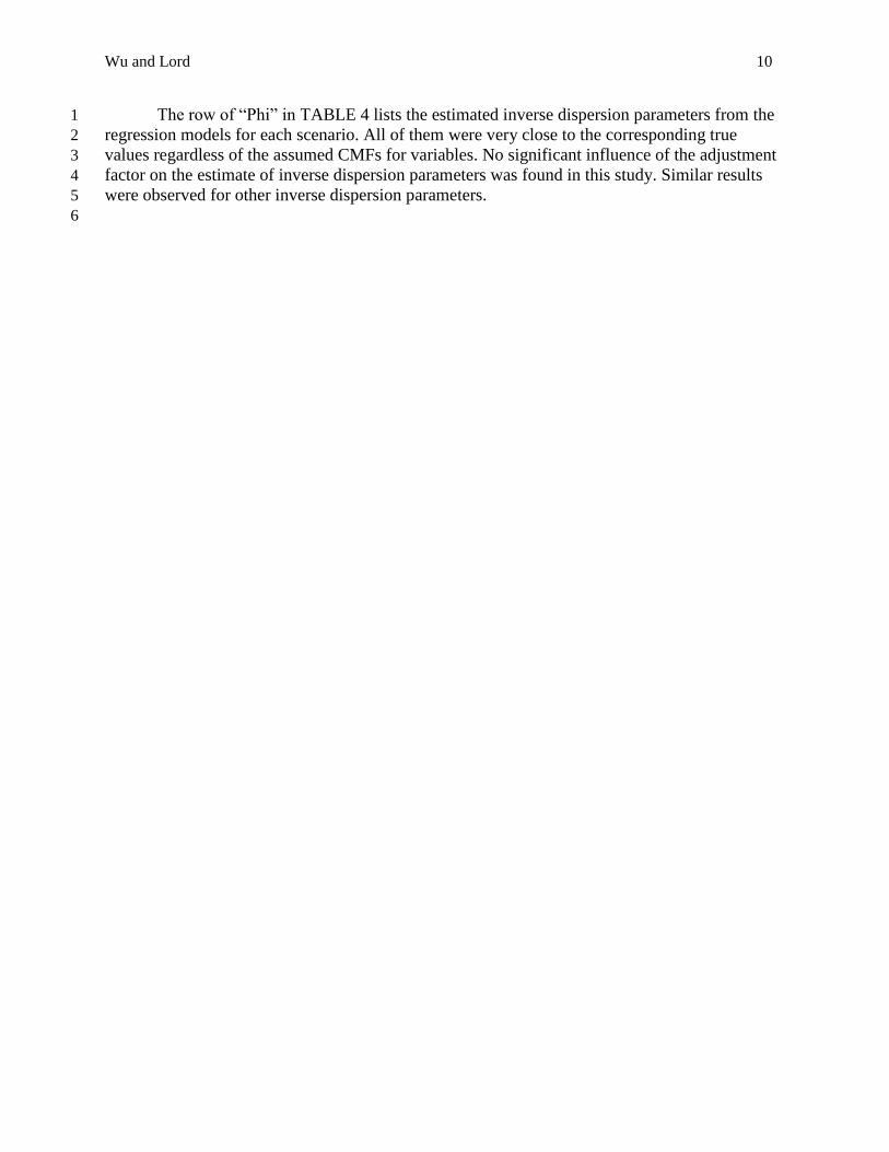
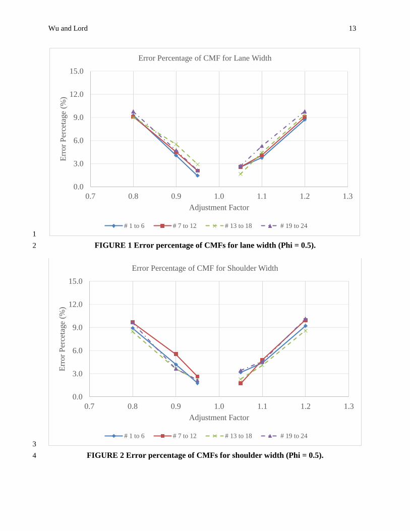
Further, the relationship between the accuracy of CMFs and the presumed adjustment 22

factors were investigated. The relationship between error percentage and adjustment factor are 23

illustrated in FIGURES 1 and 2. FIGURE 1 shows the error percentage of CMFs for lane width 24

and FIGURE 2 shows that for shoulder width. The two figures clearly indicate that the error 25

percentage was highly related to the adjustment factor. The error percentage was consistently the 26

highest when the adjustment factor was 0.80 or 1.20. And the lowest when it was 0.95 or 1.05. 27

The error percentage became small as the adjustment factor became closer to 1.0. A special case 28

can be seen when the adjustment factor equaled to 1.0, the scenario configuration fell into that in 29

Scenario II (with two variables) of the previous study (16). The error percentage should be much 30

lower (close to zero) based on the findings in that study. So the adjustment factor considerably 31

influenced the CMFs for both lane width and shoulder width. When it was close to 1.0, this 32

influence might be minor. But when it became far from 1.0 (i.e., less than or more than 1.0), the 33

accuracy of CMFs can be significantly affected. The further away it is from 1.0, the lower is the 34

quality of the CMFs. In other words, the CMFs were biased when the multiple treatments were 35

actually not affecting crash risk independently. The rate at which the value became biased was 36

actually very high when the adjustment factor went away from 1.0. 37

Wu and Lord 10

The row of “Phi” in TABLE 4 lists the estimated inverse dispersion parameters from the 1

regression models for each scenario. All of them were very close to the corresponding true 2

values regardless of the assumed CMFs for variables. No significant influence of the adjustment 3

factor on the estimate of inverse dispersion parameters was found in this study. Similar results 4

were observed for other inverse dispersion parameters. 5

6

Wu and Lord 11

TABLE 4 Results of CMFs for Lane Width and Shoulder Width (Phi = 0.5)

# AF a

LW b SW b

Phi b AIC d MAD e MSPE f Theo

SPF

(SD) Bias E Theo

SPF

(SD) Bias E

1 0.80 0.8 0.73

(0.048) -0.07 9.26 0.85

0.77

(0.046) -0.08 8.92 0.49 8750.40 0.052 0.014

2 0.90 0.8 0.77

(0.047) -0.03 4.06 0.85

0.81

(0.048) -0.04 4.19 0.50 8908.33 0.043 0.012

3 0.95 0.8 0.79

(0.049) -0.01 1.46 0.85

0.83

(0.046) -0.02 1.77 0.49 8917.64 0.040 0.010

4 1.05 0.8 0.82

(0.05) 0.02 2.57 0.85

0.88

(0.05) 0.03 3.17 0.50 9056.37 0.039 0.010

5 1.10 0.8 0.83

(0.054) 0.03 3.77 0.85

0.89

(0.054) 0.04 4.44 0.49 9106.98 0.044 0.012

6 1.20 0.8 0.87

(0.047) 0.07 8.72 0.85

0.93

(0.052) 0.08 9.20 0.50 9200.09 0.051 0.014

7 0.80 0.9 0.82

(0.043) -0.08 9.08 0.85

0.77

(0.049) -0.08 9.68 0.50 9046.82 0.055 0.016

8 0.90 0.9 0.86

(0.046) -0.04 4.50 0.85

0.8

(0.044) -0.05 5.55 0.49 9162.17 0.043 0.011

9 0.95 0.9 0.88

(0.049) -0.02 2.08 0.85

0.83

(0.048) -0.02 2.64 0.50 9223.60 0.042 0.011

10 1.05 0.9 0.92

(0.045) 0.02 2.57 0.85

0.86

(0.045) 0.01 1.76 0.49 9307.60 0.040 0.009

11 1.10 0.9 0.94

(0.055) 0.04 4.11 0.85

0.89

(0.049) 0.04 4.80 0.50 9366.01 0.043 0.010

12 1.20 0.9 0.98

(0.06) 0.08 9.04 0.85

0.93

(0.05) 0.08 9.95 0.50 9451.37 0.054 0.015

13 0.80 0.8 0.73

(0.035) -0.07 9.00 0.9

0.82

(0.047) -0.08 8.48 0.49 8927.76 0.054 0.016

14 0.90 0.8 0.76

(0.046) -0.04 5.51 0.9

0.87

(0.047) -0.03 3.66 0.50 9003.28 0.042 0.011

Wu and Lord 12

Table 4 Continued

# AF a

LW b SW b

Phi b AIC d MAD e MSPE f Theo

SPF

(SD) Bias E Theo

SPF

(SD) Bias E

15 0.95 0.8 0.78

(0.04) -0.02 2.92 0.9

0.88

(0.047) -0.02 2.19 0.49 9072.50 0.038 0.009

16 1.05 0.8 0.81

(0.045) 0.01 1.65 0.9

0.92

(0.055) 0.02 2.31 0.49 9184.27 0.041 0.009

17 1.10 0.8 0.84

(0.046) 0.04 4.45 0.9

0.94

(0.051) 0.04 4.11 0.49 9232.53 0.041 0.009

18 1.20 0.8 0.87

(0.057) 0.07 9.33 0.9

0.98

(0.054) 0.08 8.58 0.49 9330.62 0.053 0.014

19 0.80 0.9 0.81

(0.05) -0.09 9.75 0.9

0.81

(0.048) -0.09 9.64 0.51 9155.48 0.058 0.018

20 0.90 0.9 0.86

(0.044) -0.04 4.74 0.9

0.87

(0.047) -0.03 3.64 0.50 9287.17 0.044 0.011

21 0.95 0.9 0.88

(0.047) -0.02 2.13 0.9

0.88

(0.053) -0.02 2.18 0.50 9358.16 0.042 0.010

22 1.05 0.9 0.92

(0.058) 0.02 2.70 0.9

0.93

(0.055) 0.03 3.43 0.51 9447.52 0.044 0.012

23 1.10 0.9 0.95

(0.049) 0.05 5.29 0.9

0.94

(0.053) 0.04 4.60 0.49 9490.10 0.044 0.011

24 1.20 0.9 0.99

(0.061) 0.09 9.80 0.9

0.99

(0.054) 0.09 10.12 0.50 9627.21 0.056 0.016

Note: # - scenario number; a – AF is the assumed adjustment factor; b – LW is for lane width, SW is for shoulder width, Theo means

the true CMF value, SPF is the mean of CMFs from 100 experiments, SD is the standard deviation of the 100 CMFs, E is error

percentage (%); c - the mean of inverse dispersion parameter estimated from 100 experiments; d, e, f – each is the mean of the

corresponding GOF of the 100 results.

Wu and Lord 13

1

FIGURE 1 Error percentage of CMFs for lane width (Phi = 0.5). 2

3

FIGURE 2 Error percentage of CMFs for shoulder width (Phi = 0.5). 4

0.0

3.0

6.0

9.0

12.0

15.0

0.7 0.8 0.9 1.0 1.1 1.2 1.3

Err

or

Per

ceta

ge

(%)

Adjustment Factor

Error Percentage of CMF for Lane Width

# 1 to 6 # 7 to 12 # 13 to 18 # 19 to 24

0.0

3.0

6.0

9.0

12.0

15.0

0.7 0.8 0.9 1.0 1.1 1.2 1.3

Err

or

Per

ceta

ge

(%)

Adjustment Factor

Error Percentage of CMF for Shoulder Width

# 1 to 6 # 7 to 12 # 13 to 18 # 19 to 24

Wu and Lord 14

Another interesting finding from this study was the GOF measurements. Both MAE and 1

MSPE were relatively small in each scenario, and they were very close to those in the previous 2

study (16). This indicated that the predicated crash number was quite close to the true crash 3

mean. However, this did not guarantee the quality of CMFs derived from regression models, as 4

has been described above. That is to say, although the fitting result seems to be good in terms of 5

GOF measurements, there can still be some substance issues with the models. A possible reason 6

is that some parameters may have been overestimated (or underestimated) while others may have 7

been underestimated (or overestimated) in the regression models. Take Scenario 1 as an 8

example. The specific theoretical function for generating crash counts is shown in Equation 8. 9

12 612 64

, 2.67 10 0.8 0.85i iLW SWi ii i

I LW I SWLW SW

true i i iN L AADT AF (8a) 10

Or equivalently, 11

12 6

, 0.103 0.16( 0.22 )i iLW SWi iI LW I SW

itrue i i i iAF SWN L AADT exp LW (8b) 12

Where, 13

12iiLW

I LW

= indicator function for lane width of segment i. It equals to 0 if the lane 14

width is 12 ft, otherwise 1.0, and, 15

6iiSW

I SW

= indicator function for shoulder width of segment i. It equals to 0 if the 16

shoulder width is 6 ft, otherwise 1.0. 17

The modeling output of one experiment in this scenario is shown in TABLE 5. It can be 18

seen that the coefficients for lane width and shoulder width were both obviously underestimated. 19

And that for AADT was slightly underestimated. But the intercept coefficient was overestimated. 20

Note that the specific theoretical value for the intercept is not directly given in TABLE 5 due to 21

the fact that it depends on the two indicator functions. In other words, the theoretical intercept 22

varied when the segment group changed. For segment Groups 1, 2 and 3, it was -2.27 (logarithm 23

of 0.103). But it was -2.49 (logarithm of the product of 0.103 and AF, 0.8) for segment Group 4. 24

The coefficient estimated from regression models was much higher than either of them. In this 25

experiment, the coefficients for lane width and shoulder width were both underestimated. It 26

seems the underestimation was compensated through overestimating the intercept coefficient. 27

Perhaps this explains the overall smaller MAE and MSPE values. 28

Wu and Lord 15

TABLE 5 Modeling Output of the an Experiment in Scenario 1 (Phi=0.5, NB Model) 1

Model Variable Theo. Value a Coef. Value b SE c p-Value

Intercept [ 0( )ln ] -2.27-0.223ILWISW d -1.810 0.713 0.0111

Ln(AADT) ( 1 ) 1.00 0.981 0.040 < 2e-16

Lane Width ( 2 ), ft -0.223 -0.352 0.045 3.26E-15

Shoulder Width ( 3 ), ft -0.162 -0.321 0.045 6.18E-13

AIC 8921.8

MAD 0.050

MSPE 0.014

a – theoretical value; b – estimated coefficient value; c – SE is standard error; 2

d –The theoretical value for intercept was calculated by taking the nature logarithm of the first 3

two terms of Equation 8b, 12 60.103i iLW SWi i

I LW I SWAF . ILW and ISW are the two indicator 4

functions of lane width and shoulder width, respectively. 5

6

CONCLUSIONS AND DISCUSSIONS 7

This paper has documented an extensive study on the validation of developing CMFs using 8

cross-sectional studies, particularly focusing on the independence assumption (i.e., variables 9

were influencing crashes independently) with the most commonly used regression models. The 10

main objective was to examine the accuracy of CMFs estimated from regression models when 11

the independence assumption cannot be satisfied. Two variables, lane width and shoulder width, 12

were considered in this study. And an adjustment factor was used to capture the dependence 13

between the two. An adjustment factor higher than 1.0 represents widening the two at the same 14

time will reduce fewer crashes than the sum of the individuals. And vice versa if the factor is 15

lower than 1.0. Various safety effects and adjustment factors for the two variables were assumed 16

and the accuracy of CMFs were evaluated using similar approach in the authors’ previous study 17

(16). The main conclusions are summarized as follows: (1) the commonly used regression 18

models can produce biased CMFs if the considered variables influence crashes dependently; 19

(2) the bias is highly correlated with the adjustment factor (i.e., degree of the dependence of 20

variables). When the factor is close to 1.0, indicating the dependence is weak, the bias of CMFs 21

derived using regression models is relatively small, and the CMFs may still be acceptable. 22

However, higher or lower adjustment factor reduces the quality of CMFs significantly; and 23

(3) the coefficients for both treatments of interests and other variables may be over- and/or 24

underestimated under the conditions of dependent variables. The dependence relationship may be 25

absorbed into the estimates of coefficients for other variables. In one example of this study, the 26

estimated intercept coefficient was overestimated, while the coefficients for the two variables 27

were underestimated. 28

The findings in this study raised cautions to safety analysts while developing CMFs or 29

modeling crashes with multiple variables. It is recommended to examine the dependence of 30

variables. If they potentially have significant overlap in reducing crashes (i.e., the independent 31

assumption is not matched), the CMFs for individual variables derived from the SPFs are much 32

Wu and Lord 16

likely to be biased. One may ask how to examine whether two countermeasures are independent 1

or not when dealing with real crash data. Admittedly, it is not easy to conclude whether or how 2

much two or more safety treatments are dependent of each other with limited studies on the 3

safety effects of multiple treatments. Therefore, more analyses on the combined safety effects are 4

needed in the future. Before enough solid theoretical supports are available, engineering 5

judgment and experiences may need to be considered. 6

There are a few limitations with this study. First, several aspects can influence the 7

modeling result and hence the CMFs, such as the functional form and the error distribution of the 8

statistical model, sample size, etc. (4; 16; 27-30). This study only considered the most frequently 9

used one, the NB model with a linear relationship between variables, and the sample size was 10

assumed to be large enough. Second, only two variables were used and such models may be 11

influenced by the omitted-variable bias in practice. In addition, their correlation was not 12

considered, which could potentially influence the results (31). To estimate reliable CMFs, these 13

questions need further consideration when dealing with real observed data. Finally, this study 14

only raised the problem that might affect the quality of CMFs derived using regression models. 15

Safety practitioners may be more interested in solutions to this problem. So, more sophisticated 16

approaches that can assess the overlap effects of multiple treatments need to be developed in the 17

future. 18

19

REFERENCES 20

[1] Richard, K. R., and R. Srinivasan. Separation of Safety Effects of Multiple Improvements by 21

Alternate Empirical Bayes Methods. Transportation Research Record: Journal of the 22

Transportation Research Board, No. 2236, 2011, pp. 27-40. 23

[2] Carter, D., R. Srinivasan, F. Gross, and F. Council. Recommended Protocols for Developing 24

Crash Modification Factors. http://www.cmfclearinghouse.org/collateral/CMF_Protocols.pdf. 25

Accessed June 26, 2014. 26

[3] Hauer, E. Trustworthiness of Safety Performance Functions.In the 93rd Annual Meeting of 27

the Transportation Research Board (TRB), Transportation Research Board, Washington, D.C., 28

2014. 29

[4] Lord, D., and F. Mannering. The Statistical Analysis of Crash-Frequency Data: A Review 30

and Assessment of Methodological Alternatives. Transportation Research Part A, Vol. 44, No. 31

5, 2010, pp. 291-305. 32

[5] Hauer, E. Cause and Effect in Observational Cross-Section Studies on Road Safety.In the 33

84th Annual Meeting of the Transportation Research Board (TRB), Transportation Research 34

Record, Washington D.C., 2005. 35

[6] Hauer, E. Cause, Effect and Regression in Road Safety: A Case Study. Accident Analysis & 36

Prevention, Vol. 42, No. 4, 2010, pp. 1128-1135. 37

[7] Hauer, E. The Art of Regression Modeling in Road Safety. Springer, 2015. 38

Wu and Lord 17

[8] Hauer, E. Fishing for Safety Information in Murky Waters. Journal of Transportation 1

Engineering, Vol. 131, No. 5, 2005, pp. 340-344. 2

[9] Davis, G. A. Accident Reduction Factors and Causal Inference in Traffic Safety Studies: A 3

Review. Accident Analysis & Prevention, Vol. 32, No. 1, 2000, pp. 95-109. 4

[10] AASHTO. Highway Safety Manual. American Association of State Highway and 5

Transportation Officials, Washington, D.C., 2010. 6

[11] Gross, F., A. Hamidi, and K. Yunk. Issues Related to the Combination of Multiple Cmfs. 7

Presented at the 91st Annual Meeting of the Transportation Research Board, Washington D.C., 8

2012. 9

[12] Elvik, R. An Exploratory Analysis of Models for Estimating the Combined Effects of Road 10

Safety Measures. Accident Analysis & Prevention, Vol. 41, No. 4, 2009, pp. 876-880. 11

[13] Park, J., M. Abdel-Aty, and C. Lee. Exploration and Comparison of Crash Modification 12

Factors for Multiple Treatments on Rural Multilane Roadways. Accident Analysis & Prevention, 13

Vol. 70, 2014, pp. 167-177. 14

[14] Park, J., M. Abdel-Aty, J. Lee, and C. Lee. Developing Crash Modification Functions to 15

Assess Safety Effects of Adding Bike Lanes for Urban Arterials with Different Roadway and 16

Socio-Economic Characteristics. Accident Analysis & Prevention, Vol. 74, 2015, pp. 179-191. 17

[15] Park, J., and M. Abdel-Aty. Assessing the Safety Effects of Multiple Roadside Treatments 18

Using Parametric and Nonparametric Approaches. Accident Analysis & Prevention, Vol. 83, 19

2015, pp. 203-213. 20

[16] Wu, L., D. Lord, and Y. Zou. Validation of Crash Modification Factors Derived from Cross-21

Sectional Studies Using Regression Models. Presented at the 94th Annual Meeting of the 22

Transportation Research Board (TRB), Washington D.C., 2015. 23

[17] CMFClearinghouse. Installation of Fixed Combined Speed and Red Light Cameras. 24

http://www.cmfclearinghouse.org/study_detail.cfm?stid=401. Accessed July 23, 2015. 25

[18] Harkey, D. L., R. Srinivasan, J. Baek, F. M. Council, K. Eccles, N. Lefler, F. Gross, B. 26

Persaud, C. Lyon, E. Hauer, and J. A. Bonneson. Accident Modification Factors for Traffic 27

Engineering and Its Improvements. Washington, D.C. : Transportation Research Board, 28

Washington, D.C., 2008. 29

[19] Bonneson, J., and D. Lord. Role and Application of Accident Modification Factors in the 30

Highway Design Process. Report FHWA/TX-05/0-4703-2, Texas Tranportation Institute, 31

College Station, TX, 2005. 32

[20] Roberts, P., and B. Turner. Estimating the Crash Reduction Factor from Multiple Road 33

Engineering Countermeasures. Presented at 3rd International Road Safety Conference, Perth, 34

Australia, 2007. 35

Wu and Lord 18

[21] Gross, F., and A. Hamidi. Investigation of Existing and Alternative Methods for Combining 1

Multiple Cmfs. 2

http://www.cmfclearinghouse.org/collateral/Combining_Multiple_CMFs_Final.pdf. Accessed 3

July 14, 2015, 2015. 4

[22] Park, J., and M. Abdel-Aty. Development of Adjustment Functions to Assess Combined 5

Safety Effects of Multiple Treatments on Rural Two-Lane Roadways. Accident Analysis & 6

Prevention, Vol. 75, 2015, pp. 310-319. 7

[23] De Pauw, E., S. Daniels, T. Brijs, E. Hermans, and G. Wets. To Brake or to Accelerate? 8

Safety Effects of Combined Speed and Red Light Cameras. Journal of safety research, Vol. 50, 9

2014, pp. 59-65. 10

[24] Wang, X., T. Wang, A. Tarko, and P. J. Tremont. The Influence of Combined Alignments 11

on Lateral Acceleration on Mountainous Freeways: A Driving Simulator Study. Accident 12

Analysis & Prevention, Vol. 76, 2015, pp. 110-117. 13

[25] Bauer, K., and D. Harwood. Safety Effects of Horizontal Curve and Grade Combinations on 14

Rural Two-Lane Highways. Transportation Research Record: Journal of the Transportation 15

Research Board, No. 2398, 2013, pp. 37-49. 16

[26] Lord, D., S. D. Guikema, and S. R. Geedipally. Application of the Conway-Maxwell-17

Poisson Generalized Linear Model for Analyzing Motor Vehicle Crashes. Accident Analysis & 18

Prevention, Vol. 40, No. 3, 2008, pp. 1123-1134. 19

[27] Lord, D. Modeling Motor Vehicle Crashes Using Poisson-Gamma Models: Examining the 20

Effects of Low Sample Mean Values and Small Sample Size on the Estimation of the Fixed 21

Dispersion Parameter. Accident Analysis & Prevention, Vol. 38, No. 4, 2006, pp. 751-766. 22

[28] Lord, D., and L. F. Miranda-Moreno. Effects of Low Sample Mean Values and Small 23

Sample Size on the Estimation of the Fixed Dispersion Parameter of Poisson-Gamma Models for 24

Modeling Motor Vehicle Crashes: A Bayesian Perspective. Safety Science, Vol. 46, No. 5, 2008, 25

pp. 751-770. 26

[29] Wu, L., Y. Zou, and D. Lord. Comparison of Sichel and Negative Binomial Models in Hot 27

Spot Identification. Transportation Research Record: Journal of the Transportation Research 28

Board, No. 2460, 2014, pp. 107-116. 29

[30] Zou, Y., L. Wu, and D. Lord. Modeling over-Dispersed Crash Data with a Long Tail: 30

Examining the Accuracy of the Dispersion Parameter in Negative Binomial Models. Analytic 31

Methods in Accident Research, Vol. 5–6, 2015, pp. 1-16. 32

[31] Wu, L. Examining the Use of Regression Models for Developing Crash Modification 33

Factors.In the Zachry Department of Civil Engineering, Doctoral Dissertation, Texas A&M 34

University, College Station, TX, 2016. 35

36