investigating the drivers of vertical movement patterns in ...€¦ · patterns in predatory...
TRANSCRIPT

Investigating the drivers of vertical movement
patterns in predatory pelagic fishes
by
Samantha Andrzejaczek
BMSc James Cook University, BSc (Hons) University of Western Australia
This thesis is presented for the degree of Doctor of Philosophy of The University of Western
Australia
Faculty of Engineering and Mathematical Sciences
Oceans Graduate School
2018


iii
Thesis Declaration
I, Samantha Andrzejaczek, certify that:
This thesis has been substantially accomplished during enrolment in the degree.
This thesis does not contain material which has been submitted for the award of any other degree
or diploma in my name, in any university or other tertiary institution.
No part of this work will, in the future, be used in a submission in my name, for any other degree
or diploma in any university or other tertiary institution without the prior approval of The
University of Western Australia and where applicable, any partner institution responsible for the
joint-award of this degree.
This thesis does not contain any material previously published or written by another person,
except where due reference has been made in the text and, where relevant, in the Declaration that
follows.
The work(s) are not in any way a violation or infringement of any copyright, trademark, patent,
or other rights whatsoever of any person.
The research involving animal data reported in this thesis was assessed and approved by The
University of Western Australia Animal Ethics Committee. Approval #RA/3/100/1437
The following approvals were obtained prior to commencing the relevant work described in this
thesis: Permit numbers 2881 (WA Department of Fisheries) and 08-000322-3 (WA Department
of Parks and Wildlife.
This research is supported by an Australian Government Research Training Program (RTP)
Scholarship.
This thesis contains published work and/or work prepared for publication, some of which has
been co-authored.
Signature:

iv

v
Abstract
Large fishes (>30 kg adult size) of the epipelagic zone of the oceans and coastal seas display a
variety of patterns of vertical movement. Although advances in the affordability and
sophistication of electronic tags now allows researchers to routinely document these patterns, we
lack a standardised approach to classify these behaviours and to investigate their physical and
biological drivers. Here, we review the existing knowledge of the vertical movements of large,
epipelagic fishes and the evidence for the underlying factors that structure this behaviour. Using
data from both recovered satellite and biologging tags, we further investigate the drivers of these
patterns on large- (days to months) and fine- (minutes to hours) scales. Depth and temperature
archives recorded over deployment periods of up to 333 days by satellite tags allowed us to
examine how the external thermal environment influenced vertical movement behaviours in
oceanic whitetip sharks (Carcharhinus longimanus). Warming sea surface temperatures and the
stratification of the water column during summer months marked the onset of reverse
thermoregulatory strategies in this species, where changes in depth distribution and vertical
behaviours reduced their exposure to the warmest external temperatures. Biologging tags
deployed on tiger (Galeocerdo cuvier) and sandbar (Carcharhinus plumbeus) sharks for periods
of up to 48 hours recorded physical parameters including depth and temperature, and through the
use of tri-axial sensors, in-situ measurements of animal trajectory and locomotion. This enabled
calculation of dive geometry, swimming energetics and the cost of transport for these species at
fine spatial scales (m-km). Both species oscillated continually through the water column and data
from tri-axial sensors revealed shallow dive angles and gliding behaviour. Oscillations at these
fine temporal scales appear to be driven by the need to reduce the cost of transport while searching
for food, with observed inter-specific differences likely to be a function of foraging strategy.
Collectively, the drivers responsible for patterns of vertical movement depended on the temporal
scale of the sampling. I argue that characteristic patterns of vertical movement, particularly
oscillatory descents and ascents, result from the need for ram-ventilating animals to move
continuously in a three dimensional environment while optimising food encounter rates, energy
expenditure, and remaining within the limits imposed by the physical environment on their
physiology (notably water temperature).

vi
Acknowledgements
First and foremost a huge thank you goes to my supervisors Dr. Mark Meekan, Dr. Adrian Gleiss
and Prof. Charitha Pattiaratchi for their support and guidance. Mark, I cannot begin to describe
how much I have learnt from you over the last 4+ years. My writing abilities and presentation
skills would not be half of what they are today without your supervision and direction. Thank you
for opening your door to all of my problems large and small, no matter how busy you were. Also
a big thank you for all of the amazing fieldwork and travel opportunities, including my first acting
job on Shark Week (I’m still waiting on that Oscar though); some of the stories from that trip in
particular will always stay with me. Adrian, thank you for being such a brilliant supervisor,
mentor, friend and fellow ocean nerd. You showed me it is possible to be a successful marine
scientist and parent while being able to enjoy weekend adventures at the same time. I’m also so
grateful for the field opportunities you provided me with, especially the chance to fulfil a lifelong
dream and work on Blue Planet II. Chari, thank you for always being excited about my results,
and for providing a completely different perspective to my ideas. To all of my supervisors, despite
you telling me over and over that after the next trip I would be ‘chained to the desk’ until my
thesis was done, you always allowed me to go on ‘one last trip’. I still firmly believe all of the
extra trips kept me sane and productive enough to complete my thesis in the end. I’m also very
grateful for the continued support through the many ups and down, including broken bones, car
accidents and gear malfunctions.
Many collaborators and co-authors have contributed to this thesis. Karissa Lear, you have been
an amazing collaborator, labmate, travel buddy, mentor and friend. You were the best volunteer
I’ve ever had on a trip. Thank you so much for taking over my field trip responsibilities when I
broke my leg. Dr. Luciana Ferreira, you were another amazing mentor and shark nerd, thank you
for making the transition into PhD life so smooth. Thanks to Dr. Nikolai Liebsch for the
invaluable assistance with tag functioning, and always being available and patient. Thanks to Dr.
Lance Jordan, Lucy Howey and Dr. Edd Brooks for letting me have access to such an incredible
dataset for Chapter 3. Thanks to Dr. Taylor Chapple for generously letting me use your tags and
tagging pole, and getting me started on my tagging adventures. Thanks to Dr. Mauvis Gore and
Prof. Rupert Ormond for having me for an incredible month attempting to tag basking sharks. We
may not have tagged any, but it was an invaluable experience learning about academic life and
basking sharks, and giving me the opportunity to swim with my first ever basking shark. To
Kathryn Jeffs, Leon Deschamps, Shayne Thomson, Dan Paris and Nick Pedrocchi, Shark Bay
was an experience I will never forget. Kathryn – you are a force to be reckoned with.
To the amazing volunteers who gave up their time to help me either collect or analyse data -
Frazer McGregor, Abraham Sianipar, Adam Jolly, Blair Bentley, Evan Byrnes, Garry Teesdale,

vii
Michael Tropiano and Olivia Seeger. Abam, Evan, Jolly, Garry, Tropi and Karissa – that month
at Coral Bay stands out as the best month of my PhD. Thank you for making it so easy to lead my
first fieldtrip. Abam, Evan and Jolly – afternoons at ‘Grovy’ post-tagging will forever stay with
me. To all of the sharks I tagged and had the opportunity to study so closely – you are awesome.
To Lauren, Em, Steph, Dani, and Brigit, thanks for proof-reading and helping me retain some
level of sanity in those hectic last two weeks. To Lauren in particular – you are an absolute saint
and superstar.
I would not have been able to produce this thesis without the generous support of the institutions
that have provided funding and field assistance in obtaining data for this research. My gratitude
goes to the Australian Government for my PhD Scholarship, and the University of Western
Australia for the Top-Up scholarship. Thanks to BigWave Productions for having me on the
amazing trip to Cobourg Marine Park, and for providing me with my camera tags that made my
subsequent tagging trips so successful. Thanks to the Holsworth Wildlife Research Endowment
for allowing me to purchase my own diary tags, and helping me have such a long and productive
field trip to Coral Bay. Thanks to the Experiment platform for allowing me to crowdfund for my
field trips, and to the 68 kind souls who donated money to my cause. Thanks to the UWA
Postgraduate Student Association fieldwork award for also making this possible. I’m also grateful
to the UWA Graduate Research School, the Convocation of UWA Graduates, Save Our Seas, the
Australian Society of Fish Biology and KAUST for travel support allowing me to get to
conferences and workshops all around the world.
To my fellow marine nerds at UWA: Lauren, Emily, Luciana, Steph, Conrad, Phillipa, Blair,
Milly, Matty Rees, Becks, Tarryn, Claire, Dani, Jon, Brigit, Anna, Michele, Paul, Sahira,
Yannick, Chenae, Anita, Charli, Todd, Lucy, Jess, Matt H, Fernanada and Mike, thank you for
such a supportive and fun office environment. To my Murdoch family Karissa, Evan, Olly, Lauran
and Jenna – thanks for the family dinners and fun times outside of the ‘fancy’ UWA world. Brigit,
thanks for being a breath of fresh air to the office, and for being such an excellent editor. Michele
and Paul, thanks for all of the advice, morning teas, pizza nights and carpooling. Bec Wellard,
thanks for making my first PhD fieldtrip such a fun one. You opened my eyes to a world of marine
megafauna outside of sharks, and taught me so much about running my own field trips and
asserting myself. Thanks for being such a kind and genuine friend. Lauren and Emily – I don’t
think I could’ve done this without you both. Thanks for all of the coffees, wines, chocolate runs,
laughs, surfs, dives and nerd chats.
A huge thankyou to the support of my friends outside of the marine science world – the
Scarborough girls, the heaps cool stuff group, and my Flamily housemates. Katrina, Kate, Chen
and Claire - your good vibes, food and garage workouts never failed to eliminate the stress of
PhD life. Your generosity also helped me to survive off more than just canned tuna and baked

viii
beans. Katrines – forever my diving buddy. Thank you for reading through so much of my work
and always being there for me. Mother Kate – I will never be able to thank you enough for what
a kind, generous and thoughtful friend you are.
A big thanks to everyone in the Indian Ocean Marine Research Centre who helped everything run
smoothly. Thanks to Olwyn and Louise for your support. To James Gilmour, Miles Parsons and
Kimbo, thanks for always checking up on me on all of those early mornings. Thanks to Ruth and
Lara for helping with the logistics of travel and getting forms signed in time.
To everyone I met at conferences, thank you for supplying me with endless inspiration and
motivation.
An infinite thankyou to my oldest friends and family. Julia, Elysha and Ashleigh, thanks for your
unconditional friendship, life advice and support. To my mum Tina and dad Chris, thank you for
the weekly dinners, endless support, and for letting me be whatever I wanted to be. I have no
doubt that your love of the beach and Rottnest Island got me to where I am today. To my brother
Dean, thank you for being my stable rock and bank throughout my student life, and supporting
my adventures and choice of lifestyle, no questions asked. To Sal and Tones, thanks for the life
advice and the amazing dinners throughout the last three months.
Lastly, to my high school careers councillor who told me that as a marine biologist I’d end up in
the lab studying microscopic organisms, this one’s for you.

ix
Table of Contents
Thesis Declaration ....................................................................................................................... iii
Abstract ........................................................................................................................................ v
Acknowledgements ..................................................................................................................... vi
Table of Contents ........................................................................................................................ ix
Publications from this thesis ..................................................................................................... xiii
Statement of candidate contributions ........................................................................................ xiv
Co-author authorisation .............................................................................................................. xv
List of Figures ......................................................................................................................... xviii
List of Tables ............................................................................................................................ xxii
Chapter 1 General Introduction ........................................................................................... 25
1.1 Biological drivers ................................................................................................ 26
1.2 Physical drivers ................................................................................................... 27
1.3 Large, epipelagic fishes ....................................................................................... 28
1.4 Thesis aims .......................................................................................................... 28
1.5 Thesis outline ...................................................................................................... 29
Chapter 2 Patterns and drivers of vertical movements of the large fishes of the
epipelagic ............................................................................................................ 31
2.1 Abstract ............................................................................................................... 31
2.2 Introduction ......................................................................................................... 31
2.3 Methods ............................................................................................................... 33
2.4 Definitions and complexities in defining patterns of vertical movement ........... 34
2.4.1 Complexities in documenting vertical movement patterns ................................. 34
2.5 Patterns and drivers of vertical movements ........................................................ 37
2.5.1 Fine-scales (sub-second to hours) ....................................................................... 37
2.5.2 Daily scales ......................................................................................................... 40
2.5.3 Monthly scales .................................................................................................... 43
2.5.4 Seasonal scales .................................................................................................... 44
2.5.4.1 Water column structure ............................................................................... 44
2.5.4.2 Reproductive mode ...................................................................................... 45
2.5.5 Annual scale ........................................................................................................ 46
2.6 Future directions ................................................................................................. 46
2.6.1 Multi-tagging approaches.................................................................................... 47
2.7 Conclusion .......................................................................................................... 50
2.8 Acknowledgements ............................................................................................. 50
2.9 Supporting information ....................................................................................... 51

x
Chapter 3 Temperature and the vertical movements of oceanic whitetip sharks
Carcharhinus longimanus ................................................................................... 57
3.1 Abstract ............................................................................................................... 57
3.2 Introduction ......................................................................................................... 57
3.3 Materials and methods ........................................................................................ 59
3.3.1 Data collection .................................................................................................... 59
3.3.2 Data analysis ....................................................................................................... 60
3.3.2.1 Environmental parameters ........................................................................... 60
3.3.2.2 Vertical movement behaviours .................................................................... 60
3.3.2.3 Generalised linear mixed models ................................................................ 60
3.3.2.4 Breakpoint analysis ..................................................................................... 61
3.3.2.5 Multivariate analysis – hierarchical clustering ............................................ 61
3.4 Results ................................................................................................................. 62
3.4.1 Track summary ................................................................................................... 62
3.4.2 Oscillatory diving behaviours and environmental conditions ............................. 62
3.4.3 Vertical behavioural breakpoints ........................................................................ 65
3.4.4 Cluster analysis ................................................................................................... 66
3.4.5 Inter-individual variability .................................................................................. 69
3.5 Discussion ........................................................................................................... 70
3.6 Acknowledgements ............................................................................................. 73
3.7 Supporting information ....................................................................................... 74
Chapter 4 Biologging tags reveal the fine-scale movement behaviours of tiger sharks ...... 79
4.1 Abstract ............................................................................................................... 79
4.2 Introduction ......................................................................................................... 79
4.3 Methods ............................................................................................................... 81
4.3.1 Ethics ................................................................................................................... 81
4.3.2 Data collection .................................................................................................... 82
4.3.3 Data processing and analysis .............................................................................. 83
4.3.3.1 Depth record ................................................................................................ 83
4.3.3.2 Tri-axial sensor data .................................................................................... 86
4.3.3.3 Recovery period .......................................................................................... 86
4.3.3.4 Shark heading and pseudo-track calculation ............................................... 86
4.3.3.5 Window size and statistics .......................................................................... 87
4.3.3.6 Video analysis ............................................................................................. 87
4.3.3.7 Movement classification .............................................................................. 88
4.3.3.8 Generalised linear mixed models (GLMMs) ............................................... 88
4.4 Results ................................................................................................................. 88
4.4.1 Vertical movements ............................................................................................ 89
4.4.2 Horizontal path tortuosity ................................................................................... 89
4.4.3 Oscillations and tortuosity .................................................................................. 93

xi
4.5 Discussion ........................................................................................................... 94
4.5.1 Foraging behaviour and tortuosity ...................................................................... 94
4.5.2 Three-dimensional movements ........................................................................... 95
4.5.3 Challenges and future considerations .................................................................. 95
4.5.4 Conclusion .......................................................................................................... 96
4.6 Acknowledgements ............................................................................................. 96
4.7 Supporting Information ....................................................................................... 98
Chapter 5 Depth dependent dive kinematics suggest cost-efficient foraging strategies
by tiger sharks ................................................................................................... 106
5.1 Abstract ............................................................................................................. 106
5.2 Introduction ....................................................................................................... 106
5.3 Methods ............................................................................................................. 108
5.3.1 Ethics ................................................................................................................. 108
5.3.2 Data collection .................................................................................................. 108
5.3.3 Data processing ................................................................................................. 110
5.3.3.1 Gliding behaviour ...................................................................................... 110
5.3.3.2 Ascent and descent speed .......................................................................... 110
5.3.3.3 Window size and statistics ........................................................................ 111
5.3.4 Data analysis ..................................................................................................... 111
5.3.4.1 Generalised linear mixed models (GLMMs) ............................................. 111
5.3.4.2 Cost of transport models ............................................................................ 112
5.4 Results ............................................................................................................... 114
5.4.1 Track summary ................................................................................................. 114
5.4.2 Gliding behaviour ............................................................................................. 115
5.4.3 Relationship between seabed depth and vertical movement behaviours .......... 115
5.4.4 Cost of transport models ................................................................................... 117
5.5 Discussion ......................................................................................................... 120
5.5.1 Cost of vertical movements ............................................................................... 120
5.5.2 Cost-efficient foraging ...................................................................................... 121
5.5.3 Model limitations .............................................................................................. 122
5.5.4 Seascape effects on energy expenditure and gain ............................................. 122
5.5.5 Conclusion ........................................................................................................ 123
5.6 Acknowledgements ........................................................................................... 123
5.7 Supplementary information ............................................................................... 125
Chapter 6 First insight into the fine-scale movement behaviours of sandbar sharks
Carcharhinus plumbeus .................................................................................... 127
6.1 Abstract ............................................................................................................. 127
6.2 Introduction ....................................................................................................... 127
6.3 Materials and methods ...................................................................................... 128
xii
6.3.1 Data collection .................................................................................................. 128
6.3.2 Data processing ................................................................................................. 130
6.3.2.1 Depth Record ............................................................................................. 130
6.3.2.2 Tri-axial sensor data .................................................................................. 130
6.3.2.3 Shark heading and pseudo-track calculation ............................................. 131
6.3.2.4 Window size and statistics ........................................................................ 131
6.3.2.5 Video analysis ........................................................................................... 132
6.3.3 Statistical analysis ............................................................................................. 132
6.4 Results ............................................................................................................... 133
6.4.1 Vertical movements .......................................................................................... 133
6.4.2 Tortuosity and three-dimensional paths ............................................................ 137
6.4.3 Video ................................................................................................................. 139
6.5 Discussion ......................................................................................................... 140
6.5.1 Tortuous circling behaviour .............................................................................. 140
6.5.2 Vertical movements .......................................................................................... 141
6.5.3 Species comparisons ......................................................................................... 141
6.5.4 Limitations and future considerations ............................................................... 142
6.5.5 Conclusions ....................................................................................................... 143
6.6 Acknowledgements ........................................................................................... 143
6.7 Supporting Information ..................................................................................... 144
Chapter 7 General Discussion ........................................................................................... 147
7.1 Seasonal scales of vertical movement ............................................................... 148
7.2 Biologging and fine-scale patterns of vertical movement ................................. 149
7.3 Temporal scale and vertical movements ........................................................... 151
7.4 Limitations and future directions ...................................................................... 151
7.5 Implications ....................................................................................................... 153
7.6 Concluding remarks .......................................................................................... 155
Bibliography ............................................................................................................................. 156
Appendix A .............................................................................................................................. 172

xiii
Publications from this thesis
Chapter 2
Andrzejaczek S, Gleiss AC, Pattiaratchi CB, Meekan MG. In Review. Patterns and drivers of
vertical movements of the large fishes of the epipelagic. Reviews in Fish Biology and Fisheries.
Chapter 3
Andrzejaczek S, Gleiss AC, Jordan LKB, Pattiaratchi CB, Howey LA, Brooks EJ, Meekan MG
(2018) Temperature and the vertical movements of oceanic whitetip sharks, Carcharhinus
longimanus. Scientific Reports 8:8351
Chapter 4
Andrzejaczek S, Gleiss AC, Lear KO, Pattiaratchi CB, Chapple T, Meekan MG (In preparation).
Biologging tags reveal the fine-scale movement behaviours of tiger sharks.
Chapter 5
Andrzejaczek S, Gleiss AC, Lear KO, Pattiaratchi CB, Chapple T, Meekan MG (In preparation).
Depth dependent dive kinematics suggest cost-efficient foraging strategies by tiger sharks.
Chapter 6
Andrzejaczek S, Gleiss AC, Pattiaratchi CB, Meekan MG (2018b) First insight into the fine-scale
movement behaviours of sandbar sharks Carcharhinus plumbeus. Frontiers in Marine Science 5
xiv
Statement of candidate contributions
This thesis is presented as a series of five manuscripts in journal formats, as well as the general
introduction and general discussion sections. These papers were developed by my own ideas and
hypotheses with inputs from my supervisors.
Dr. Lance Jordan (Microwave Telemetry), Lucy Howey (Microwave Telemetry) and Dr Edd
Brooks (Cape Eleuthera Institute) contributed recovered tag data for Chapter 3. I deployed tags
at Ningaloo Reef for Chapters 4, 5 and 6.
Fieldwork for Chapter 4, 5 and 6 was supported by a Holsworth Wildlife Research Endowment,
crowdfunding on the Experiment platform (DOI: 10.18258/7190), the University of Western
Australia, the UWA Graduate Research School, the Australian Institute of Marine Science, Coral
Bay Research Station and BigWave Productions.
The analyses described in all data chapters were carried out by myself and all chapters were
written by me with feedback from Dr Mark Meekan (all chapters), Dr Adrian Gleiss (all chapters),
Prof Charitha Pattiaratchi (all chapters), Dr Lance Jordan (Chapter 3), Lucy Howey (Chapter 3),
Dr Edward Brooks (Chapter 3), Karissa Lear (Chapter 4 and 5) and Dr Taylor Chapple (Chapter
4 and 5).

xv
Co-author authorisation
This thesis contains work that has been published and prepared for publication. By signing below,
co-authors agree to the listed publication being included in the candidate’s thesis and
acknowledge that the candidate is the primary author, i.e. contributed greater than 50% of the
content and was primarily responsible for the planning, execution and preparation of the work for
publication.
Details of the work:
Andrzejaczek S, Gleiss AC, Pattiaratchi CB, Meekan MG. In Review. Patterns and drivers
of vertical movements of the large fishes of the epipelagic. Reviews in Fish Biology and
Fisheries.
Location in thesis:
Chapter 2: Patterns and drivers of vertical movements of the large fishes of the epipelagic
Student contribution to work:
I conducted the review of the literature, created all plots, and wrote the manuscript with
criticial input from co-authors.
Co-author signatures and dates:
Dr. Mark Meekan Dr. Adrian Gleiss Prof. Charitha Pattiaratchi
26.11.2018 26.11.18 26.11.18
Details of the work:
Andrzejaczek S, Gleiss AC, Jordan LKB, Pattiaratchi CB, Howey LA, Brooks EJ, Meekan
MG (2018) Temperature and the vertical movements of oceanic whitetip sharks,
Carcharhinus longimanus. Scientific Reports 8:8351
Location in thesis:
Chapter 3: Temperature and the vertical movements of oceanic whitetip sharks,
Carcharhinus longimanus.
Student contribution to work:
I analysed the data and wrote the manuscript with critical input from co-authors.
Dr. Mark Meekan Dr. Adrian Gleiss Prof. Charitha Pattiaratchi
26.11.18 26.11.18 26.11.18
Dr. Lance Jordan Dr. Edward Brooks Miss Lucy Howey
3/10/2018 3/10/2018 2/10/2018

xvi
Details of the work:
Andrzejaczek S, Gleiss AC, Lear KO, Pattiaratchi CB, Chapple T, Meekan MG (In
preparation). Biologging tags reveal the fine-scale movement behaviours of tiger sharks.
Target journal: Marine Biology
Location in thesis:
Chapter 4: Biologging tags reveal the fine-scale movement behaviours of tiger sharks.
Student contribution to work:
I collected and analysed the data and wrote the manuscript with critical input from co-
authors.
Co-author signatures and dates:
Dr. Mark Meekan Dr. Adrian Gleiss Prof. Charitha Pattiaratchi
26.11.18 26.11.18 26.11.18
Dr. Taylor Chapple Miss Karissa Lear
27.11.18 26.11.18
Details of the work:
Andrzejaczek S, Gleiss AC, Lear KO, Pattiaratchi CB, Chapple T, Meekan MG (In
preparation). Depth dependent dive kinematics suggest cost-efficient foraging strategies by
tiger sharks.
Location in thesis:
Chapter 5: Depth dependent dive kinematics suggest cost-efficient foraging strategies by
tiger sharks
Student contribution to work:
I collected and analysed the data and wrote the manuscript with critical input from co-
authors.
Co-author signatures and dates:
Dr. Mark Meekan Dr. Adrian Gleiss Prof. Charitha Pattiaratchi
26.11.18 26.11.18 26.11.18
Dr. Taylor Chapple Miss Karissa Lear
27.11.18 26.11.18

xvii
Details of the work:
Andrzejaczek S, Gleiss AC, Pattiaratchi CB, Meekan MG (2018) First insight into the
fine-scale movement behaviours of sandbar sharks Carcharhinus plumbeus. Frontiers in
Marine Science 5
Location in thesis:
Chapter 6: First insight into the fine-scale movement behaviours of sandbar sharks
Carcharhinus plumbeus
Student contribution to work:
I collected and analysed the data and wrote the manuscript with critical input from co-
authors.
Co-author signatures and dates:
Dr. Mark Meekan Dr. Adrian Gleiss Prof. Charitha Pattiaratchi
26.11.18 26.11.18 26.11.18
Student signature
Date: 26.11.18
I, Professor Charitha Pattiaratchi certify that the student’s statements regarding their
contribution to each of the works listed above are correct.
Coordinating supervisor signature:
Date: 26.11.18
xviii
List of Figures
Figure 2.1. Schematic diagrams of the major patterns of vertical movements found in
large epipelagic fishes: (a) Swimming at a constant depth; (b) Surface
oriented single deep dives; (c) bottom oriented single deep dives; (d)
oscillatory swimming; (e) normal diel vertical migration; (f) reverse diel
vertical migration; and (g) diel changes in oscillatory swimming ...................... 35
Figure 2.2. Relationship between the reported maximum duration of tag attachment
(days) and the maximum recorded depth (meters) in a tagging study. Each
dot in the scatterplot corresponds to a peer-reviewed study on a pelagic
predatory fish. The trendline depicts the logarithmic relationship, with the
shaded area displaying error bars. N=120, R2=0.24. ........................................... 36
Figure 2.3. Swim and glide movements of whale sharks at Ningaloo Reef. Ascents show
significant locomotory activity (lateral acceleration) while descents were
largely passive (i.e. gliding). Figure reproduced from Gleiss et al. (2011a). ...... 40
Figure 2.4. Schematic diagram of positive and negative thermotaxis in an epipelagic fish. ..... 43
Figure 2.5. Two tiger sharks (i & ii) with very similar oscillatory depth tracks but
different horizontal tracks in offshore environments over a 2.5 hour period.
(a) Depth track. (b) Pseudo-track. C) 3D track. See Chapter 4 for detail on
how these tracks were derived. ........................................................................... 48
Figure 3.1. Schematic diagrams of (a) hypothetical performance curve of an ectotherm
adapted from Huey and Stevenson (1979). The curve describes the
temperature for which performance is optimised (Topt) and the critical
minimum and maximum temperatures (Tcritmin and Tcritmax) at which an
organism can survive; and (b) the cyclic characteristics of oscillatory
movements; mean cycle length and cycle amplitude were extracted from a
continuous wavelet transformation on depth data. .............................................. 59
Figure 3.2. (a) Vertical movements of a tagged oceanic whitetips over the course of 11
months. (b) The monthly mean temperature range between the surface and
100 meters depth for tagged oceanic whitetips. The red and blue shaded
bars indicate timing of northern hemisphere summer and winter
respectively. ........................................................................................................ 63
Figure 3.3. Daily oscillatory behaviour in a (a) winter and (b) summer water column for
OWT8, and (c) winter and (d) summer for OWT7. Temperatures are
averaged for the months of February and September respectively for 10 m
depth bins. Depth trace is a 24-hour track sampled at a two minute
frequency. Note that temperature scale-bars are not consistent between
individual sharks. ................................................................................................ 63
Figure 3.4. Relationship between SST and (a) daily % of time spent in the top 50 m and
(b) daily mean cycle length (s). Red and blue lines display results of
piecewise regression with the blue line indicating the breakpoint, and the
red lines the linear relationship either side of this breakpoint. ............................ 65
Figure 3.5. Results from multivariate analysis of daily data where SST >28°C. Input
variables were daily values of proportion of time spent in the top 50 m,
mean depth, mean cycle length and mean amplitude. (a) Dendrogram of
vertical movement behaviour determined from hierarchical cluster analysis.
(b) The two principal components scores are plotted for daily data. Points
are coloured by their cluster group. ..................................................................... 67
xix
Figure 3.6. 24-hour depth profiles representative of each group derived from the
hierarchical cluster analysis. a) Medium % top 50, medium cycles, low
amplitude, b) low % top 50, long cycles, low amplitude, c) medium % top
50, long cycles, medium amplitude, d) low % top 50, short cycles, low
amplitude, e) high % top 50, short cycles, low amplitude, f) medium % top
50, long cycles, high amplitude. Note that the scale on the y-axis differs for
Cluster 6. ............................................................................................................. 68
Figure 3.7. The percentage of time each individual OWT spent in each calculated cluster.
The x-axis is ordered based on similarity of cluster composition between
OWTs. OWT11, OWT13 and OWT16 were excluded from this analysis
due to insufficient sample size in days with SST>28°C...................................... 69
Figure 4.1. Tagged tiger sharks at Ningaloo Reef. (a) Tiger shark post-release. Photo
courtesy of Alex Kydd. (b) CATS Cam tag clamped to the dorsal fin. (c)
CATS Diary tag clamped to the dorsal fin. (d) Location of tag
deployments. ....................................................................................................... 82
Figure 4.2. Comparison of dominant vertical movement clusters (V-groups) and path
tortuosity clusters (T-groups) from hierarchical cluster analysis. (a) 15
minute depth profiles representative of V-groups 1, 3 and 6, demonstrating
the increase in oscillatory movements with V-group. (b) 15 minute pseudo-
tracks representative of each T-group, demonstrating the increase in
tortuosity with T-group. Polar plot on bottom right of each track displays
example of heading variance for each group. (c) The % windows found in
each cluster. (d) The % T-group composition of each dominant V-group.
Colours are T-groups from (b). ........................................................................... 90
Figure 4.3. Tiger shark and loggerhead turtle interaction. (a) One-hour long pseudo-track
from TS15. Red square denotes area of prey interaction displayed in (b)
and (c). (b) Depth track. (c) 3D track. (d) Screenshots from video of the
interaction. 1 and 2 refer to where interaction takes place in depth and 3D
tracks. See Supplementary Video 1 for full video of interaction. ....................... 91
Figure 4.4. One minute pseudo-tracks of tiger shark and Chinamanfish (Symphorus
nematophorus) interactions. Track line is coloured by tailbeat frequency
(Hz). Red dashed square indicates where the fish was observed in the video
field of view (displayed in screenshots to the right of the pseudo-track). X
and Y-axes represent arbitrary units of latitude and longitude created by
magnetometer and accelerometer data whilst a constant speed is assumed.
(a) Example of an interaction where the tailbeat of the shark slows upon
encountering the fish. (b) Example of an interaction where the tailbeat of
the shark quickens upon encountering the fish. .................................................. 92
Figure 4.5. Two tiger sharks (i & ii) with very similar oscillatory depth tracks but
different horizontal tracks in offshore environments over a 2.5 hour period.
(a) Depth track. (b) Pseudo-track. (c) 3D track. .................................................. 93
Figure 4.6. 15 minute pseudo-track throughout a tortuous window in TS20. Track is
coloured by bursts (ODBA>0.2) and takes place at approximately 21:30 in
water approximately 2 m in depth. ...................................................................... 93
Figure 5.1. Location of tagging and tag recoveries. Note that eight tags are outside of the
map area – two approximately 10 km further north, and six offshore
(ranging from 15-27 km offshore). ................................................................... 109
Figure 5.2. Schematic representation of an oscillatory movement, and the distance
parameters used in calculating the cost of transport. ........................................ 113

xx
Figure 5.3. Mean instantaneous ODBA for all 21 tiger sharks at a range of absolute (a)
ascent and (b) descent angles (placed in 5° bins). All sharks displayed a
positive slope for ODBA ~ ascent angle. No consistent relationship was
found between ODBA and descent angle. Unique symbols and/or colours
represent individual tiger sharks. ...................................................................... 114
Figure 5.4. Gliding in tiger sharks over the course of A) an entire track (10 hours); B) 45
minutes; and C) 6 minutes. Glides are marked in red on the x axis.
Dynamic angular velocity was taken from the lateral (sway) axes recorded
by the gyroscope. D) The proportion of descent time spent gliding by each
individual tiger shark. ....................................................................................... 116
Figure 5.5. Relationship between dive angle and habitat depth. (a & b) Boxplots
displaying differences in ascent and descent pitch angle between habitat
zones. Inshore denotes areas where maximum depth within a window was
<25 m, and offshore where depths were >25 m. Shark silhouettes angles
are not to scale. (c & d) Relationship between maximum depth in a
sampling window and descent and ascent angle in inshore zones (<25 m). ..... 118
Figure 5.6. (a) Relationship between seabed depth (m) and diving ratio measured in 15
minute windows. Maximum depth is a proxy for seabed depth. The red line
displays diving ratio calculated if time level swimming at the surface and
seabed for oscillations remained the same at all maximum depths. (b, c)
Schematic diagrams representing how diving ratio may differ as a result of
seabed depth and sampling window. Depth traces have the same vertical
velocity, and same time spent level swimming at the surface and seabed in
between vertical movements. (c) Represents a habitat of twice the depth of
habitat (b). Red dashed square represents the fixed time window within
which diving ratio is measured. ........................................................................ 119
Figure 5.7. The cost of transport of a single oscillatory movement of a tiger shark on (a) a
horizontal plane and (b) a vertical plane. Arrows indicate where the cost of
transport is minimised in both cases. Lines represent the cost of a given
descent pitch angle (label on figure) in relation to varying ascent pitch (x-
axis). .................................................................................................................. 120
Figure 6.1. Tagged sandbar sharks at Ningaloo Reef. (a) Location of tag deployments (b)
CATS Cam tag clamped to the dorsal fin. (c) CATS Diary tag clamped to
the dorsal fin...................................................................................................... 129
Figure 6.2. Gliding behaviour in a tagged sandbar shark (Shark 3) over the course of
approximately 30 minutes. Dynamic angular velocity was taken from the
lateral (sway) axes recorded by the gyroscope. Glides are marked where
the mask analysis determined gliding was occurring. ....................................... 134
Figure 6.3. Entire depth record and gliding behaviour for each tagged sandbar shark.
Glides are marked where the mask analysis determined gliding was
occurring. Dashed blue squares denote extended periods of U-shaped
diving, and associated looping behaviour. (a) Shark 1; (b) Shark 2; (c)
Shark 3; and (d) Shark 4. Note that both x- and y-axes scales differ
between sharks. ................................................................................................. 136
Figure 6.4. U-shaped dives and looping behaviour in Shark 1. (a) Depth record displaying
U-shaped dives in the late afternoon and dusk. Red square denotes 15
minute period of looping behaviour displayed in (c) and (d). (b) Pseudo-
track. (c) 3D track. (d) Screenshot of Shark 1 swimming at the seabed on
the bottom phase of a U-shaped dive. Shark silhouette indicates direction
of travel by shark. Note that the x and y-axes in (b) and (c) represent
arbitrary units of latitude and longitude as they were created by dead-
reckoning using magnetometer and accelerometer data assuming a constant
speed. ................................................................................................................ 138
xxi
Figure 6.5. 15 minute pseudo-tracks of looping behaviour from each sandbar individual
around dusk. (A) Shark 1 at 17:30 at depth 36 m; (B) Shark 2 at 18:08 at
depth 67 m; (C) Shark 3 at 17:47 at depth 67 m; and (D) Shark 4 at 17:42
at depth 15 m. .................................................................................................... 138
Figure 6.6. Five minute 3D tracks and pseudo-tracks of turning behaviour throughout the
ascents and descents of U-shaped dives and V-shaped dives. X and Y axes
represent arbitrary units of latitude (P-lat) and longitude (P-long) as they
were created by dead-reckoning using magnetometer and accelerometer
data assuming a constant speed. The Z axes in the 3D plots represents
depth (m). .......................................................................................................... 139
Figure 7.1. Schematic of the timeline of different processes that may influence patterns of
vertical movement in large, epipelagic fishes. Dashed squares denote the
time periods for which biologging tags and recovered satellite tags will be
most effective. ................................................................................................... 147
Figure S 3-1. The relationship between daily averaged vertical movement behaviours and
SST for each individual OWT. (a) Mean daily depth; (b) percentage time in
the top 50 m; (c) mean cycle length (seconds); and (d) mean amplitude. ........... 78
Figure S 4-1. Recovery period in tiger sharks after being caught and released. Black dots
and error bars represent mean tailbeat cycles (the inverse of tailbeat
frequency) during descent for individual tiger sharks over 15 minute
windows. The solid blue line is the combined regression for all individuals,
and the red dashed line indicates the point at which the approximate 80%
threshold was calculated, and individuals were considered to be recovered.
Methods follow that of Whitney et al. (2016b) ................................................... 98
Figure S 4-2. Video validation of seabed. A) Entire depth track from TS24. B) & C)
Excerpts of TS24 track displaying where seabed was observed on video. ......... 99
Figure S 4-3. Interaction between a tiger shark and turtle in the sandflats around Coral
Bay. Photos courtesy of Daniel Thomas-Browne. ............................................ 100
Figure S 5-1. Relationships between dive angles and maximum depth; (a) Maximum
depth and ascent angle for all data. (b) Maximum depth and descent angle
for all data only. ................................................................................................ 125
Figure S 6-1. Mean and sd of tailbeat cycles (inverse of tailbeat frequency) during descent
for individual sandbar sharks over 15 minute windows. (a) Shark 1; (b)
Shark 2; (c) Shark 3; and (d) Shark 4. ............................................................... 144
Figure S 6-2. Relationship between diving ratio and sum of turning angles for each
individual sandbar shark. .................................................................................. 145
Figure S 6-3. Confounding movements into deeper water and increasing tailbeat cycle in
Shark 2. (A) Entire depth trace in Shark 2; (B) Mean and sd of tailbeat
cycle (seconds) during descent for Shark 2. Red line outlines time of
movement into deeper water and increasing tailbeat cycle length. ................... 145
xxii
List of Tables
Table 2-1. Performance of commonly used tag types. Satellite refers to data transmitted to
user through satellites. Data-logger refers to short deployment biologging
tags. Poor Average Good *Will depend on if setting up a new
receiver array, or working within an existing network. ...................................... 35
Table 3-1. Subset of model comparisons using Akaike's Information Criterion (AIC),
Bayesian Information Criterion (BIC) and conditional (R2c) and marginal
(R2m) R2 values. ΔAIC displays deviance in AIC scores from top-ranked
models. All models are generalised linear mixed models and were ran
using the nlme package in R with shark identity as a random variable.
Proportion of time spent in the top 50 m (Prop50) was logit transformed
prior to analysis. All null models include the random effect. To see all
models involved in the model selection process, see Table S 3.2. ...................... 64
Table 3-2. Mean (± standard deviation) of daily vertical movement behaviours above and
below 28°C. ......................................................................................................... 66
Table 3-3. Summarised characteristics of each cluster derived from the hierarchical
cluster analysis. Values are mean ± standard deviation. ..................................... 67
Table 4-1. Terms and definitions used repetitively throughout chapter ..................................... 81
Table 4-2. Summary details of tagged tiger sharks. *Tag malfunction, no data
downloaded **Tag shut off before detachment nResight – same as TS17.......... 84
Table 4-3. Results of generalised linear mixed models testing the relationship between
diving ratio and indicators of horizontal path tortuosity. Diving ratio was
logit transformed prior to analysis. All models were compared with null
models using Akaike’s Information Criterion (AIC) and conditional (R2c)
and marginal (R2m) R2 values. All models were run using the nlme
package in R with shark identity as a random variable. All null models
include the random effect .................................................................................... 92
Table 5-1. Results of generalised linear mixed models testing the relationship between
seabed depth (MaxD) and vertical movement behaviours. All models were
compared with null models using Akaike’s Information Criterion (AIC)
and conditional (R2c) and marginal (R2m) R2 values. All models were run
using the nlme package in R with shark identity as a random variable. All
null models include the random effect. Inshore indicates windows where
maximum depth was <25 m, and offshore where maximum depth was >25
m. ...................................................................................................................... 117
Table 6-1. Summary details of tagged sandbar sharks. CC: CATS Camera tag, CD: CATS
Diary tag ............................................................................................................ 134
Table 6-2. Summary statistics calculated for the entire dataset, and each tagged
individual. Statistics were firstly calculated for 15 minute windows, then
summarised for the entire tagging duration. TBF: tailbeat frequency, VV:
Vertical velocity, 𝑹: mean circular length. ....................................................... 135
Table 6-3. Linear model comparisons using Akaike’s Information Criterion (AIC), R2,
and p-values. ΔAIC displays deviance in AIC scores from null model.
Diving ratio is modelled as a function of turning, where turning is the sum
of the turning angles for a sampling window. Model results where turning
is standardised by vertical phase of movement are shown in Supplementary
Table 1............................................................................................................... 137

xxiii
Table S 2.1. Reported biological characteristics and vertical movement behaviours (as
defined in section 1) in large predatory epipelagic fishes. indicates that
the behaviour was observed in at least one study for the species,
indicates that the behaviour was not observed. *Species does not meet
criteria for large, predatory epipelagic fish, but retained in table for
comparison. **Maximum number of long-term archived datasets reported
to be recovered in a single study. ........................................................................ 51
Table S 3.1. Summary of tagging information and biological information of the tagged
individuals. .......................................................................................................... 74
Table S 3.2. All models involved in the model selection process. Model comparisons
were made using Akaike's Information Criterion (AIC), Bayesian
Information Criterion (BIC) and conditional (R2c) and marginal (R2m) R2
values. ΔAIC displays deviance in AIC scores from top-ranked models. All
models are generalised linear mixed models and were ran using the nlme
package in R with shark identity as a random variable. Proportion of time
spent in the top 50 m (Prop50) was logit transformed prior to analysis. All
null models include the random effect. ............................................................... 75
Table S 3.3. Results from proportion time top 50 m ~ mean SST breakpoint analysis.
Breakpoints were assessed for the full dataset and each individual shark.
Model comparisons were made using Akaike's Information Criterion (AIC)
between models with and without the breakpoint term. ΔAIC displays
deviance in AIC scores between these two models. *Calculated breakpoint
not robust............................................................................................................. 76
Table S 3.4. Results from mean cycle length ~ mean SST breakpoint analysis.
Breakpoints were assessed for the full dataset and each individual shark.
Model comparisons were made using Akaike's Information Criterion (AIC)
between models with and without the breakpoint term. ΔAIC displays
deviance in AIC scores between these two models. *Calculated breakpoint
not robust. **Breakpoint term significantly improves model. ............................ 76
Table S 4.1. Ethogram used in the video analysis in BORIS (Behavioural Observation
Research Interactive Software; Friard and Gamba 2016). ................................ 101
Table S 4.2. Summarised characteristics of each V-group derived from the hierarchical
cluster analysis. Values are mean ± standard deviation. ................................... 102
Table S 4.3. Summarised characteristics of each T-group derived from the hierarchical
cluster analysis. Values are mean ± standard deviation. ................................... 103
Table S 4.4. All predator-prey interactions recorded on CATS video tags .............................. 103
Table S 5.1. Estimated ascent and descent speeds calculated by pitch and vertical velocity
for absolute dive angles >20° for each individual tiger shark, and their
relationship with pitch. Individuals with <20 points were excluded (TS10,
TS16, TS20, TS25). Note that where significant relationships exist, slopes
do not exceed an absolute value of 0.02. .......................................................... 126
Table S 6.1. Linear model comparisons using Akaike’s Information Criterion (AIC), R2,
and p-values. ΔAIC displays deviance in AIC scores from null model.
Diving ratio (DR) is modelled as a function of turning. Turning has been
subset for each vertical phase of movement (level swimming, ascending
and descending), and standardised by the time spent in that phase within a
sampling window. ............................................................................................. 146


25
Chapter 1 General Introduction
Movement, at the scale of an organism, is defined as a change in the spatial location of the whole
individual in time (Nathan et al. 2008). A holistic understanding of this process necessitates
research into the patterns, drivers, physiology and consequences of animal movement;
collectively encompassing the field of movement ecology (Nathan et al. 2008; Hays et al. 2016).
Throughout the lifetime of an organism, movement patterns will be driven by a number of
processes that interact across multiple spatial and temporal scales. Drivers can be either physical
(e.g. temperature, oxygen availability) or biological (e.g. prey density, predator avoidance)
(Schlaff et al. 2014). By understanding how these factors shape movements, we will have a better
capacity to predict how environmental change may alter the distribution of organisms in space
and time, and make more informed management decisions (Hussey et al. 2015).
In recent decades, rapid advances in tagging technologies and our increasing ability to analyse
large datasets has resulted in an exponential increase in the description of patterns of animal
movement, particularly those of megafauna (Hussey et al. 2015; Kays et al. 2015). A focus on
megafauna stems from both the logistical and ethical constraints of attaching tags to individuals
of a minimum size, as well as the importance associated with understanding the movements of
these animals (Kays et al. 2015; Estes et al. 2016). Megafauna, defined by Estes et al. (2016) as
species reaching >45 kg maximum reported mass, are typically wide-ranging, triggering large
energy transfers between spatially distinct habitats, and need to consume large quantities of
biomass. As a result, they influence trophic dynamics and potentially structurally modify the
ecosystems they inhabit through the processes of foraging and locomotion (McCauley et al. 2012;
Roman et al. 2014; Estes et al. 2016). In addition, as a result of their charismatic nature,
megafauna often have high social and economic values (O'Connor et al. 2009; Gallagher and
Hammerschlag 2011; Vianna et al. 2012; Estes et al. 2016). Large body size, however, is
correlated with a number of life history traits, such as slow growth and low reproductive rate, that
increase extinction risk in these animals (Fisher and Owens 2004; Cardillo et al. 2005). Human
exploitation of megafauna has resulted in many of these species undergoing large declines in
abundance so that the status of their populations is often classified as Endangered or Vulnerable
by the International Union for the Conservation of Nature (IUCN) Red List (IUCN 2018). Given
their trophic role, and the extent of anthropogenic threats (harvest, climate change, ocean
acidification, habitat loss etc.) that now confront them, it is imperative that we gain a better
understanding of their movement ecology if we are to effectively manage and conserve these taxa.
In marine habitats, megafauna have been tracked at a diverse range of temporal and horizontal
spatial scales (Block et al. 2011; Hussey et al. 2015). The addition of the vertical dimension of
water depth, however, complicates our understanding of movements in these environments in

26
several ways. Firstly, as physical variables have a much steeper gradient of change vertically than
horizontally (e.g. temperature, light and oxygen), disentangling the multiple interacting physical
and biological drivers of movements in this plane can be very challenging. Secondly, the vastness
of marine systems and the difficulties involved in transmitting data through water has impeded
the progress of the field of movement ecology compared to terrestrial ecosystems. Lastly, the
motivations for movements throughout three-dimensional environments can be non-intuitive to
humans, as the majority of our movements occur on a horizontal plane.
Despite these problems, we have a general understanding of the principal biological and physical
drivers that are likely to act collectively to produce the observed movement patterns of marine
megafauna. The following sections outline these drivers and how they may act individually and
synergistically to influence movements of marine megafauna.
1.1 Biological drivers
Inter- and intra-specific interactions with other individuals are a fundamental driver of movements
through the processes of foraging, predation, competition and reproduction (Hays et al. 2016).
Throughout the lifespan of an animal, it will need to move to search for sufficient prey and mates,
while minimizing detection by potential predators. Although reproductive drivers may only
influence mature individuals at seasonal scales, and species at the apex of food chains may not
need to avoid other predators (at least at adult sizes), all individuals will be driven by the need to
find food. The distribution, quality and density of prey will vary in space and time and trade-offs
may exist to optimize net energy intake across different temporal and spatial scales (Stephens and
Krebs 1986). For example, Womble et al. (2014) tracked juvenile female harbor seals (Phoca
vitulina) using time-depth recorders, real-time vessel tracking, and hydroacoustic surveys, to
investigate how prey availability in contrasting habitats influenced harbor seal diving and
foraging behaviour. The study found that individuals that made use of terrestrial haul-out sites
had shorter horizontal distances to travel to forage on high prey densities at shallower depths,
whereas seals using tidewater glacial ice sites as haul-outs had to travel further and dive deeper
to access prey that occurred at a lower density. Haul-out on glacial ice, however, was found to
offer seals a more stable resting platform and therefore greater refuge from predators. In addition,
the prey accessed by seals from these glacial sites was predicted to be of higher lipid content and
energy density (Womble et al. 2014). Thus, seals appeared to be balancing the costs and benefits
of utilising these distinct habitats, which had impacts on their movement patterns.
Despite prey distribution and density likely acting as a fundamental driver of movements of
marine megafauna, studies that provide direct and simultaneous measurements of the prey field
associated with predator movement, as described above, are rare (Hays et al. 2016). Typically,
movements are indirectly linked with foraging behaviours (e.g. Sims et al. 2006; Aguilar Soto et

27
al. 2008; Friedlaender et al. 2013). For example, the daily migration of the deep scattering layer
(DSL) into deeper and darker waters has been associated with the movements of almost all major
groups of marine megafauna, including sharks, tuna and marine mammals (Hays 2003; Musyl et
al. 2003; Sims et al. 2005; Friedlaender et al. 2013). Despite the volume of this evidence, we lack
studies that have simultaneously measured movement of both predator and prey, or of the
variation in the physical environment that either predator or prey encounter as they descend or
ascend through the water column.
Variation in biological characteristics, such as morphometry and body composition between
individuals, will influence the degree to which hydrodynamic drag affects the movements of
marine megafauna. Water is a dense and viscous medium, and forward motions are resisted by
backward-acting drag forces. As a result, hydrodynamic drag will influence the movements of
marine animals at their finest scale (Schmidt-Nielsen 1972). The energetically expensive cost of
swimming has resulted in a number of morphological and behavioural solutions to reduce the
negative effects of drag (Fish 1994; Williams et al. 2000; Gleiss et al. 2011c). To move more
efficiently through the water, marine mammals, reptiles and fish have been found to display
patterns of intermittent locomotion, whereby individuals intersperse periods of powered
locomotion with passive gliding (Williams et al. 2000; Fossette et al. 2010; Gleiss et al. 2011c).
When and where an individual glide will depend on a number of factors, including its buoyancy,
depth and instantaneous motivation for movement i.e. travel, search or hunting.
1.2 Physical drivers
Physical drivers may affect animal movements indirectly, by altering patterns of prey density and
distribution, or directly, by affecting their physiology (Schlaff et al. 2014). These drivers can
include dissolved oxygen, temperature, tide, pressure and light. For air-breathers, the most
obvious driver of movements is the need to return to the surface between dives to obtain oxygen.
Dive profile, duration and surface interval will all influence how an individual stores and
consumes oxygen while at depth (Boyd 1997; Ponganis and Williams 2015). Although gill-
breathers are not constrained by a need to return to the surface, vertical movements of individuals
may still be limited by concentrations of dissolved oxygen, which generally decline with
increasing depth. Reduced availability of oxygen may act as a barrier to movement or reduce time
available at depths where minimum levels occur (Kramer 1987; Prince and Goodyear 2006).
Environmental temperature plays a fundamental role in structuring the distribution, diversity and
movements across marine taxa (Tittensor et al. 2010). It is arguably the most influential driver
governing the movements of marine animals, particularly for ectotherms that cannot internally
regulate their body temperature (Angilletta et al. 2002). As the rate of many major physiological
functions are determined by core body temperature, the performance of ectotherms is directly

28
related to the temperature of the surrounding environment (Angilletta et al. 2002; Bernal et al.
2012). In order to maximise performance, these animals must use behavioural strategies to
thermoregulate by moving through their habitat in a manner that, on average, maintains a
preferred thermal range (Neill 1979).
Collectively, biological and physical drivers will act synergistically to produce documented
patterns of movement. Determining the influence of each driver will be complex, and dependant
on the spatial and temporal scale in question.
1.3 Large, epipelagic fishes
The relative ease in deploying tags on air-breathing and coastal marine megafauna, such as seals,
means that our understanding of the movement ecology of these animals has progressed faster
and further than that of gill-breathing, pelagic species (Wilson and Vandenabeele 2012; Schlaff
et al. 2014). In addition, fishes are not obliged to return to the surface to obtain oxygen, which
firstly complicates the classification of “dive” types and the comparison of patterns of vertical
movement both within and among species, and secondly impedes satellite tags from transmitting
data back to the end-user. To overcome these issues, studies of epipelagic fishes have traditionally
focused on horizontal, rather than vertical, patterns of movement. This has generated a critical
gap in our understanding of the movement ecology of these species. Although advances in the
affordability and sophistication of electronic tags now allows researchers to routinely document
vertical movement patterns, we lack a standardised approach to classify these behaviours and to
investigate their physical and biological drivers.
1.4 Thesis aims
The overall goal of my thesis is to understand patterns and drivers of vertical movements in large
epipelagic fishes (>30 kg adult size), with a focus on sharks. I use new analytical techniques and
advanced tagging technologies to improve our understanding of the patterns and drivers of vertical
movements of these species across a range of temporal scales. Specifically I:
1) Synthesize our current knowledge of patterns and drivers of vertical movements, and outline
future directions and research priorities.
2) Investigate how temperature drives the vertical movements of sharks on a seasonal time scale.
3) Explore the role of cost-efficient foraging in driving fine-scale vertical movements of sharks
In line with these aims, my thesis is organized into a meta-analysis chapter and four data chapters,
and the findings are drawn together in a final discussion chapter.

29
1.5 Thesis outline
In Chapter 2, I review the database of published tracking studies documenting the vertical
movement patterns of large epipelagic fishes, and discuss the available evidence to explain how
biological and physical drivers may structure these behaviours. I classify vertical patterns, and
identify the complexities in studying these movements that need to be acknowledged and
addressed in future studies. I argue that characteristic patterns of vertical movement result from
the need for ram-ventilating animals to move continuously in a three dimensional environment
while optimising food availability, energy expenditure, and remaining within the limits imposed
by the physical environment (notably water temperature and oxygen) on their physiology. I also
show that the drivers of patterns of vertical movement are dependent on the temporal scale of
observation.
At seasonal scales, epipelagic fishes may encounter changes in the physical structure of the water
column. In Chapter 3, I use depth and temperature archives from satellite tags deployed on oceanic
whitetip sharks (Carcharhinus longimanus) to investigate the role of water temperature in driving
vertical movements in this species. Spectral analysis, linear mixed modelling, segmented
regression and multivariate techniques were used to examine the effect of mean sea surface
temperature (SST) and mixed layer depth on vertical movements at seasonal scales. I discuss the
results of this study in the context of a warming ocean.
At finer scales from seconds to hours, vertical movements of epipelagic fishes are likely to be
driven by the need to optimize the energetic costs of foraging and locomotion. In Chapters 4, 5
and 6, I used biologging tags to examine the extent to which the movements of tiger (Galeocerdo
cuvier) and sandbar (Carcharhinus plumbeus) sharks were consistent with cost-efficient foraging
strategies. Tags recorded both physical parameters, and in situ measurements of animal trajectory
and locomotion, which enabled the calculation of dive geometry, swimming energetics and path
tortuosity at fine spatial scales in both species. In Chapter 4, I explore how biologging data can
be used to link vertical movements to prey-searching behaviours in tiger sharks. In Chapter 5, I
investigate the extent to which patterns of oscillatory diving by tiger sharks conform to a strategy
of cost-efficient foraging by modelling the cost of transport, and describe how habitat depth
influences the movement strategies of these animals. In Chapter 6, I integrate the methods used
in Chapters 4 and 5 to provide an initial insight into the vertical movements of sandbar sharks,
and discuss how recorded patterns conformed to cost-efficient foraging strategies.
In Chapter 7, I synthesize and integrate the findings of my thesis. I discuss how insights into
vertical movements of epipelagic fishes at multiple temporal scales can broaden our
understanding of the primary ecological and physiological drivers of these behaviours. I describe
limitations in our current understanding of vertical movements in large epipelagic fishes given

30
available technologies, and highlight future directions for research in this field. Finally, I discuss
the conservation and management implications of my results.

31
Chapter 2 Patterns and drivers of vertical
movements of the large fishes of the
epipelagic
2.1 Abstract
Large fishes (> 30 kg adult size) of the epipelagic zone of the oceans and coastal seas display a
variety of patterns of vertical movement. Although advances in the affordability and
sophistication of electronic tags now allows researchers to routinely document these patterns, we
lack a standardised approach to classify these behaviours and to investigate their physical and
biological drivers. Here, we provide a review of existing knowledge of the vertical movements of
large, epipelagic fishes and the evidence for the underlying factors that structure this behaviour.
We focus on behaviours occurring at a range of temporal scales, from seconds to days, months
and years. We argue that characteristic patterns of vertical movement result from the need for gill-
breathing animals to move continuously in a three dimensional environment while optimising
food encounter, energy expenditure and remaining within the limits imposed by the physical
environment on their physiology (notably water temperature and oxygen). Biologging
technologies that record both the internal (body temperature, heart rate, blood chemistry) and
external physical environment coupled with direct recording of behaviour from animal-borne
cameras offer a new, synthetic approach to the analysis of the interrelationships among drivers of
patterns of vertical movement. Ultimately, this can provide insights into the evolution of the
behaviour and morphology of these animals.
2.2 Introduction
Understanding the vertical movements of large, epipelagic fishes is important for a number of
reasons. Because they are highly mobile, these fishes create trophic flows through food webs by
consumption of prey and the subsequent excretion of organic material, carbon, nitrogen and other
nutrients (Bird et al. 2018; Williams et al. 2018). This process, entitled active subsidies, can link
spatially distinct habitats (McCauley et al. 2012) and is particularly important on vertical axes
because many species show regular patterns of transit between the surface and deeper waters. The
potential for nutrient and energy transfers among depths by epipelagic fishes is substantial, given
that blue (Balaenoptera musculus) and sperm (Physeter macrocephalus) whales, which consume
prey at depth and subsequently excrete faeces into the photic zone, transfer 3000 and 50 tonnes
of iron respectively into the surface waters of the iron-limited Southern Ocean each year (Lavery
et al. 2010; Lavery et al. 2014), creating a carbon sink that for sperm whales results in the export
of 4 x 10⁵ tonnes of carbon annually to the deep sea (Lavery et al. 2010). The extent to which the
32
movement patterns of epipelagic fishes contribute to similar processes of nutrient enrichment and
carbon transfer is unknown, but could be many times greater, given the higher relative abundance
of these animals (Estes et al. 2016).
Description of vertical patterns in movements is also essential for the management of fisheries
where large epipelagic fishes are caught as targets or by-catch. Tunas and billfishes form the basis
of important commercial and recreational fisheries worldwide, whereas sharks are a large part of
incidental bycatch. More recently, targeted catches of sharks and rays have provided an additional
source of income for fishers due to the high value of their fins, meat and/or gill rakers (Clarke et
al. 2006; Majkowski 2007; Braun et al. 2015; Dent and Clarke 2015; Williams and Terawasi
2015). In 2014, tuna fisheries in the western and central Pacific Ocean reported their highest-ever
catch with a record value of US$ 5.8 billion (Williams and Terawasi 2015). In 2011, the most
recent year for which full global data sets are available, the value of total world imports of shark
meat was conservatively declared at US$ 379.8 million by the FAO, well above the average
annual value for the previous decade (US$ 239.9 million) (Dent and Clarke 2015). Worldwide,
overexploitation by fishing threatens the continued existence of many stocks of epipelagic fishes
(Davidson Lindsay et al. 2015; Punt et al. 2015; Pons et al. 2016).
Determining the environmental drivers influencing vertical movements will assist in predicting
the depth distribution of epipelagic fishes, and as a result, their vulnerability to different fishing
gears. Knowledge of these factors may contribute to the sustainability of catches and to minimise
impacts on non-target species (Bigelow and Maunder 2007). It is also critical in a world facing
global climate change (Koopman et al. 2014; Schlaff et al. 2014). A warming ocean may shift the
distributions of epipelagic species to deeper waters, although the magnitude of this effect will
vary among species and habitats (Schlaff et al. 2014; Andrzejaczek et al. 2018). Conversely,
oxygen minimum zones are expected to expand and shoal with climate change, causing the
hypoxic habitat boundaries of fishes to move upwards towards the surface and to compress
available habitats (Bograd et al. 2008; Stramma et al. 2008; Prince et al. 2010).
The decline in abundance of large, predatory epipelagic fishes due to overfishing not only has
economic consequences, but also impacts the function of oceanic ecosystems through the loss of
both top-down structuring processes and risk-driven effects in food chains (Creel and
Christianson 2008; Heithaus et al. 2008). Direct predation by these fishes and their wide-ranging
nature means their removal is likely to result in trophic cascades that have complex effects in
ecosystems on large spatial and temporal scales (Stevens et al. 2000; Baum and Worm 2009;
Ferretti et al. 2010; Estes et al. 2011) (but see Grubbs et al. 2016).
In recent decades there has been a rapid increase in movement studies of large, epipelagic
predatory fishes that has been driven by technological advances in acoustic and satellite telemetry
(Hammerschlag et al. 2011; Papastamatiou and Lowe 2012; Whitney et al. 2012; Braun et al.

33
2015). New generations of electronic tags now allow researchers to record and observe the
movements of these animals at a wide range of temporal and spatial scales and in many cases,
also provide estimates of environmental parameters such as depth, temperature, light and
dissolved oxygen encountered by the tagged individual (Block et al. 2011; Hammerschlag et al.
2011). However, the majority of early tagging studies focussed on horizontal, rather than vertical,
patterns of movement (Speed et al. 2010; Thums et al. 2013), despite these animals occupying a
three-dimensional environment. This reflected the fact that for reasons of cost, studies often
deployed tags that only reported surface positions, rather than the depths of animals. The
introduction of low-cost acoustic and satellite tags that combine a variety of sensors including
depth and temperature have now made the documentation of vertical patterns in movement of
epipelagic species commonplace.
The aim of this review is to provide a synthesis of existing knowledge of the vertical movements
of large, epipelagic fishes and to provide a framework that can be used to investigate the drivers
of these patterns in future studies. This requires a number of key steps. Unlike marine mammals,
whose vertical movements depart from and ultimately return to the surface in order for animals
to breathe, fishes are not necessarily constrained to visit the surface between excursions to deeper
waters. Nonetheless, most species show patterns of oscillatory descents and ascents through the
water column at various temporal and spatial scales. In Section 1 we define movement patterns
and review some of the complexities involved in drawing general patterns from time-depth
records of epipelagic fishes. We then review the literature for examples of these patterns and
examine the evidence for the proposed biological and environmental drivers of these vertical
movements (Section 2). The final part of the review outlines a framework for use in future studies
that aim to understand the mechanisms behind these movements (Section 3). In this review, we
define large, epipelagic fishes as species that attain maximum sizes > 30 kg and spend a majority
of their lives traversing the top 0-200 m of the pelagic environment (the epipelagic). We focus
primarily on sharks, rays, tunas and billfishes, many of which are considered to be apex or top-
order predators in this environment. In association with their large size, these animals generally
have patterns of relatively low abundance, slow growth rates and late ages at maturity, increasing
their vulnerability to anthropogenic threats (Table S 2.1; Hutchings et al. 2012; Dulvy et al. 2014;
Juan-Jordá et al. 2015).
2.3 Methods
This review is based on key word and title searches of library and electronic databases using the
words ‘shark(s)’, ‘tuna(s)’, ‘vertical movement’, ‘diving behaviour’, ‘telemetry’ and ‘tagging’.
Key words cited in papers found through database searches were also incorporated. For each study
the following information was recorded: (1) study species and location; (2) telemetry technology
(or technologies); (3) length (hours-days) of track(s); (4) vertical movement behaviours

34
identified; and (5) hypothesised drivers of vertical movements. Where possible, maximum
recorded depth (meters) and maximum length of tag attachment (days) were also noted (Table S
2.1).
2.4 Definitions and complexities in defining patterns of
vertical movement
For air-breathing marine vertebrates, the departure from and return to the surface of an animal to
breathe (a “dive”) form the standard unit of analysis of patterns of vertical movement. As sharks
and other predatory fishes breathe using a gill and are not obliged to return to the surface, “dives”
are more difficult to define. However, standardisation of definitions is vital to allow for
comparisons among studies. Time-depth records can instead be used to provide data on central or
baseline depths (Womble et al. 2013), and variation around this baseline depth can be used to
classify the vertical movement patterns of large epipelagic fishes. In this review, ‘dives’ simply
refer to a steep descent from a baseline depth. Our review of the literature found four major types
of vertical movements that occurred recurrently among taxa (Figure 2.1, Table S 2.1): swimming
at a constant depth (Figure 2.1a); single deep dives (Figure 2.1b, Figure 2.1c); oscillatory
swimming (Figure 2.1d, Figure 2.1g); and diel vertical movements (Figure 2.1e, Figure 2.1f,
Figure 2.1g). However, the degree to which these patterns can be resolved depends on the tag
type and its sampling duration and frequency of recording data.
2.4.1 Complexities in documenting vertical movement
patterns
The choice of tag for deployment by a researcher will depend on the question being addressed,
and is often an attempt to achieve a balance between duration of retention on the target species,
resolution of recovered data and cost of the tag (Table 2-1). Analysis of different types of vertical
movements requires data collected at sufficient resolution by pressure sensors in tags. In many
types of satellite tags (e.g. Pop-off archival tags and SPLASH tags) data is transmitted in
summarised form, typically as frequency histograms in depth bins predetermined by the
researcher. This lowers cost and increases efficiency of transmissions due to the limited
bandwidth available for the upload of data by satellites. However, such data sets lack the
resolution required to identify detailed patterns of vertical movements. Complete time series of
depth are only available when tags are recovered after deployments and archives held within the
tag can be downloaded. Unfortunately, for most epipelagic fishes, tag recoveries remain relatively
rare events (on average less than 10% of tags deployed), unless animals are targeted in
commercial or recreational fisheries (Table S 2.1).

35
Table 2-1. Performance of commonly used tag types for recording vertical movement. Satellite refers to
data transmitted to user through satellites. Data-logger refers to short deployment biologging tags. Poor
Average Good *Will depend on if setting up a new receiver array, or working within an existing
network.
Satellite Archival Acoustic Data-logger
Deployment duration
Resolution
Probability of recovering data
Price *
Measurement of additional parameters
Figure 2.1. Schematic diagrams of the major patterns of vertical movements found in large epipelagic
fishes: (a) Swimming at a constant depth; (b) Surface oriented single deep dives; (c) bottom oriented single
deep dives; (d) oscillatory swimming; (e) normal diel vertical migration; (f) reverse diel vertical migration;
and (g) diel changes in oscillatory swimming

36
The duration, timing and location of tag attachment may affect the type and variation of vertical
movements that are identified in a data set. Tracks of longer duration provide greater opportunity
to both record infrequent events such as very deep dives (mesopelagic depths) and to document
changes in vertical movements occurring over larger temporal or spatial scales. Our analysis of
120 studies shows that an asymptotic relationship exists between maximum depth and length of
tag deployment for predatory epipelagic fishes (Figure 2.2). This relationship suggests that tags
needed to be attached to fishes for a minimum of approximately 100 days in order for very deep
dives to be documented, an attachment duration attained for 36 of the 41 species reported here.
The analysis also indicated that although dives to depths greater than 500 m may occur
infrequently, they are a ubiquitous characteristic of the vertical movements of the majority of
species included in our analysis. Due to the rarity of these deep dives, mean or median depth may
be a more informative metric for comparisons among and within taxa. Nevertheless, maximum
depths provide data on performance limits for species and may reveal new insights into
physiology and behavioural ecology (Houghton et al. 2008). However, records of maximum
depths of dives can be limited by tag technology. Depths recorded by acoustic tags will be
restricted by receiver range and the habitats where receivers are deployed and most satellite-linked
tags (e.g. PAT tags) have pressure sensor resolution and design constraints that limit records of
descents to around 2000 m depths (e.g. Wildlife Computers, USA). At present, the maximum
depths recorded for epipelagic predators are descents to 1,994 m by a swordfish (Xiphias gladius)
(Evans et al. 2014) and to 1,928 m by a whale shark (Rhincodon typus) (Tyminski et al. 2015).
As in both cases these were the depth limits of pressure sensors, it remains to be determined if
these maxima simply represent a design constraint of the tag.
Figure 2.2. Relationship between the reported maximum duration of tag attachment (days) and the
maximum recorded depth (meters) in a tagging study. Each dot in the scatterplot corresponds to a peer-
reviewed study on a pelagic predatory fish. The trendline depicts the logarithmic relationship, with the
shaded area displaying error bars. N=120, R2=0.24.

37
A lack of clear boundaries between dives, or the superimposition of different types of dives during
the same bout adds a further layer of complication to any analysis of diving. High-resolution data
sets reveal that some vertical movement behaviours can co-occur within the same dive or can alter
in frequency and amplitude over time (Figure 2.1g). For example, oscillatory dives of blue sharks
(Prionace glauca) were repeated every few hours, but were deeper in the daytime and shallower
at night (Carey et al. 1990) implying both hourly and diurnal cycles in vertical movement
behaviours. Archival tags recovered from deployments on skipjack tuna (Katsuwonus pelamis)
have revealed similar patterns (Schaefer and Fuller 2007), with regular oscillations of this species
recorded between depths of 50-300 m during the day, whereas vertical movements at night were
restricted to waters above the thermocline (44 m deep). Similarly, the amplitude of single deep
dives may change on a diel scale, or deep dives may increase in frequency to an extent that they
become classified as oscillatory movements. Diel patterns in vertical movement of a species may
also vary spatially. For example, albacore tuna (Thunnus alalunga) tagged in tropical latitudes
were found to exhibit a distinct transition from occupation of shallow, warm waters above the
depth of the mixed layer at night to deeper, cooler waters below the mixed layer during the day.
In contrast, there was no evidence of diel patterns for the same species tagged in temperate
latitudes (Williams et al. 2015a).
2.5 Patterns and drivers of vertical movements
The drivers of vertical movement patterns of large epipelagic fishes may be both physiological
and ecological, constituting the drivers setting the maximum limits to vertical distributions, and
influencing how animals may move within these limits. These may act synergistically, with the
relative importance of each dependent on temporal scale and context (Gleiss et al. 2013).
Foraging, thermoregulation, navigation and energy-saving are likely to be the key drivers of
patterns of vertical movements of many epipelagic fishes (Carey et al. 1990). Here, we examine
the evidence for consistent patterns in vertical movement and their suggested drivers among
species, studies and localities. Although the temporal scale of discrete vertical movement patterns
typically operate at hourly-daily scales, the factors driving these movements operate at scales
ranging from seconds to seasons to years. To simplify the discussion of the role of these drivers,
this section follows a temporal construct, beginning with drivers operating at fine timescales (sub-
second – hours) and concluding with those operating at annual timescales.
2.5.1 Fine-scales (sub-second to hours)
Repetitive cycles of oscillations through the water column from the surface to depth (also called
bounce or yo-yo dives; Figure 2.1d) that occur over a few minutes or hours within a diel period
are a characteristic feature of nearly all epipelagic fishes (Table S 2.1) and can occur both in
38
shallow and deep water. For example, 40 tiger sharks (Galeocerdo cuvier) tagged with animal
attached video systems (CritterCam) and acoustic tags in Shark Bay, Western Australia exhibited
oscillatory vertical movements in waters of only 6-15 m depth (Heithaus et al. 2002b). On
average, cycles of these movements occurred 14 times per hour. Whale sharks tracked at Ningaloo
Reef, Western Australia by Gleiss et al. (2011a) displayed three types of oscillatory dives, the
first of which were ‘bounce dives’, where oscillations were greater than 10 m depth in range and
began and ended near the surface, without an extended surface interval between dives. The second
was a series of ‘V-shaped dives’ where the surface interval between consecutive dives was less
than 30 minutes, and the third type was ‘small scale bottom-bounce dives’ with oscillations of
less than 10 m that occurred between the descent and ascent phases of a U-shaped dive. All these
dives occurred in waters 60-100 m deep. In deeper waters, blue sharks were documented
undergoing oscillations from the surface to 200-400 meters at 1-3.5 hour intervals (Carey et al.
1990).
Such oscillatory movements are thought to be a search strategy to detect prey, with the descent
and ascent of fishes through the water column increasing the probability of detecting cues
(olfactory, visual, electrosensory) that may reveal the presence of food (Carey et al. 1990; Klimley
et al. 2002). Despite the prevalence of this argument, very few studies have simultaneously
measured prey abundance and diving behaviours of epipelagic predatory fishes. Josse et al (1998)
tracked yellowfin (Thunnus albacares) and bigeye tuna (Thunnus obesus) using acoustic tags and
concurrently mapped deep scattering layers in the water column to in order to explore the overlap
of tuna movements with their prey. At the small spatial and temporal scales at which these were
measured (up to 24 hours), tuna appeared to display movements in association with the vertical
and horizontal distributions of prey (Josse et al. 1998).
More recently, the development of multi-sensor data-logger (biologging) tags that include
pressure sensors and accelerometers, and accompanying software and data analysis techniques
(Sakamoto et al. 2009; Walker et al. 2015) has enabled researchers to explore the extent to which
these patterns of oscillatory diving can also confer energy savings for epipelagic fishes. The
intermittent swimming hypothesis proposed by Weihs (1973), suggests that oscillatory swimming
may be utilised by negatively-buoyant animals as an energy saving tactic. Theoretically, by
gliding on descent and actively swimming on ascent, fish could generate savings of up to 50% of
locomotor energy expenditure when compared with swimming at a constant depth between two
horizontal points. The hypothesis also calculates the angles of ascent and descent at which energy
savings would be maximised when undergoing these swim-glide movements. Post-processing of
acceleration data collected from a number of different species shows results consistent with this
hypothesis. For example, Gleiss et al. (2011a) used accelerometers to assess the geometry and
power requirements of five dive types employed by whale sharks. The tagged whale sharks
predominately glided on descent and altered between shallower or steeper angles of ascent in
39
order to reduce the cost of transport on horizontal and vertical scales respectively (Figure 2.3).
Gliding behaviour appears to be a common feature of the oscillatory movements of most
epipelagic predatory fishes for which detailed data records from accelerometer tags are available
(Furukawa et al. 2011; Gleiss et al. 2011b; Gleiss et al. 2011c). This implies that both efficient
prey searching and energy saving outcomes can be combined in oscillatory vertical movements,
so that this type of diving can be a strategy for cost-effective foraging (Meekan et al. 2015;
Papastamatiou et al. 2018a). However, in most instances, the evidence for foraging behaviour
during oscillatory dives is largely inferential. For example, in the north eastern China Sea, eight
dolphinfish (Coryphaena hippurus) tagged with acceleration data-loggers glided for 83.4 ± 20.0%
of the descent phase of vertical movements (Furukawa et al. 2011). These fish remained
predominately at the surface (0-5 m depths), but made deeper dives during periods when the
thermocline was deeper in the water column, which Furukawa et al. (2011) suggested was due to
changes in the distribution of their prey, although no direct measures of food resources were made.
The recent integration of cameras into biologging tags now allows the direct observation of
interactions between epipelagic predators and their prey. Although there have been relatively few
published studies that have used this approach, research on tiger and oceanic whitetip sharks
(Carcharhinus longimanus) provides some direct evidence for a link between oscillatory
movements and prey searching. Heithaus et al. (2002b) used Crittercams to record interactions
between tiger sharks and prey in coastal waters and suggested that oscillations allowed tiger
sharks to search the seabed for prey on descent and the surface for silhouettes of prey on ascent.
Shark-borne video footage from tagged oceanic whitetip sharks showed that potential prey items
were most commonly observed during oscillatory dives and at the apex of dives (Papastamatiou
et al. 2018a). In addition, accelerometers and speed sensors showed that dives conformed to
predictions for minimising the cost of transport throughout oscillatory movements.

40
Figure 2.3. Swim and glide movements of whale sharks at Ningaloo Reef. Ascents show significant
locomotory activity (lateral acceleration) while descents were largely passive (i.e. gliding). Figure
reproduced from Gleiss et al. (2011a).
2.5.2 Daily scales
Over a cycle of 24 hours, the most common pattern in vertical movements of epipelagic fishes is
diel vertical migration (DVM), where fishes are distributed deeper or dive deeper during the day
and are distributed shallower or dive shallower at night, with shifts in depth distributions
occurring at dawn and dusk (Figure 2.1e). This pattern of behaviour is largely thought to be a
response to the DVM of the deep scattering layer (or sound scattering layer), which consists of
small fishes (mostly myctophids) and invertebrates that migrate to depth at sunrise and rise to
surface layers near the thermocline at sunset to feed. The descent of the deep scattering layer into
deeper, cooler and darker waters during the day reduces the probability of detection and
consumption by visual predators, and epipelagic fishes are thought to modify their vertical
movements to exploit these migrations (Hays 2003).
Diel patterns in vertical movement were evident in almost all large epipelagic species investigated
in this review (see Supplementary Table 1). Carey (1990) was one of the first studies to directly
link the vertical movements of an epipelagic fish with the DVM of the deep scattering layer.
Echograms revealed the descent of the deep scattering layer just before dawn, and a concurrent
track from an acoustically tagged swordfish found it to follow this migration down 10 minutes
later (Carey 1990). Given that the DVM of many epipelagic fishes mimic those of plankton, it is
perhaps not surprising that some of the clearest patterns of DVM are shown by filter-feeding
elasmobranchs. A megamouth shark (Megachasma pelagios) tracked for 50.5 hours ascended and
descended in the water column on a regular crepuscular schedule, from depths of 12-25 m at night

41
to 120-166 m in the day. (Nelson et al. 1997). Basking sharks (Cetorhinus maximus) tracked in
the English Channel displayed similar patterns of DVM, although these could reverse (shallower
during the day, deeper at night, Figure 2.1f) depending on the distribution of planktonic prey
(Sims et al. 2005).
In the open ocean and highly stratified coastal systems, this occupation of the deep scattering
layer (200-500 m) poses some important physiological challenges for epipelagic fishes as
temperatures are on average 10-20°C cooler than at the surface. As gills are very efficient heat
exchangers, blood passing through the respiratory system can quickly lose its heat to the external
environment, and body temperature can cool below optimal temperatures (Angilletta et al. 2002;
Carey et al. 1971). To alleviate this problem and maintain temperatures within a preferred range
while foraging in very cool water at depth, many epipelagic fishes have been found to perform
physiological and/or behavioural thermoregulation. Ectothermic whale sharks regularly diving to
depths of 200-500 m during the day were found to exhibit a negative relationship between mean
surface duration and the mean minimum temperature of deep dives, suggesting that these sharks
rewarm and therefore behaviourally thermoregulate at the surface. The high thermal inertia of this
very large fish may also be key in slowing cooling rates when foraging at depth (Meekan et al.
2015). Bigeye tuna occupy depths of around 250 m during the day and make episodic, rapid
vertical excursions into warm waters near the surface, and remain in these shallower waters at
night (Evans et al. 2008; Musyl et al. 2003; Schaefer and Fuller 2002). Telemetered data shows
that these endothermic fishes disengage vascular counter-current heat exchangers on ascent
during the day to allow rapid warming at the surface, and reactivate them on return to depth in
order to conserve heat (Holland et al. 1992).
The ability to conserve heat internally and maintain body temperature above ambient
(endothermy) may influence the extent to which epipelagic fishes vertically move to rewarm
while feeding at depth. Various levels of endothermy have evolved in a number of species
examined in this review, namely the tuna, billfishes, lamnid sharks, devil rays and opah (Dickson
and Graham 2004; Thorrold et al. 2014; Wegner et al. 2015). Internal thermistors provide a means
to assess the capacity of these animals to physiologically rewarm (e.g. Carey 1990; Musyl et al.
2003; Wegner et al. 2015). For example, in cooler and deeper waters, thermistors placed in the
muscle and cranial cavity of swordfish exposed the ability to slow cooling rates in these areas,
while blue shark muscle temperature cooled at a more rapid rate (Carey 1990). Swordfish were
consequently able to remain at depth in temperatures approximately 10°C below that of the
surface for up to 8 hours throughout the day, while blue sharks oscillated back to the surface every
few hours, presumably to rewarm (Carey et al. 1990; Carey 1990). Ideally, such evidence would
continue to be gathered by tags that measure internal temperatures and depth, however
deployment of such technology presents a major logistic and ethical challenge in the case of many
large predators.

42
Although many studies of vertical movements of epipelagic fishes, notably those on billfishes,
have suggested that these animals display patterns of behavioural thermoregulation such as
basking after deep diving during the day (Dewar et al. 2010; Chiang et al. 2011; Abecassis et al.
2012; Chiang et al. 2015), field evidence for such behaviours is very limited. Ideally, such
evidence would be gathered by tags that measure internal temperatures and depth (e.g. Musyl et
al. 2003; Nakamura et al. 2015a), however deployment of such technology presents a major
logistical and ethical challenge in the case of many large predators. Indirect evidence of basking
may still be available in the analysis of archived data of time-depth records using the approach of
Thums et al (2013). Alternatively, these vertical movement patterns may be a form of reverse
thermoregulation, whereby fishes close to upper thermal limits either due to very warm surface
water and/or high energy output descend in long glides into cool, deep waters to lower body
temperatures (negative thermotaxis, Figure 2.4). Dives may also serve to cool body temperatures
allowing fishes to be more active for foraging in warm surface waters. In effect, this would be the
opposite of the behaviour of basking prior to diving in order to prolong the ability to forage in
cold water at depth as occurs in species such as whale sharks (positive thermotaxis, Figure 2.4).
Given the very similar shape of these two profiles, a biologging approach may be required to test
these hypotheses as archival depth and temperature data alone may not allow for the distinction
to be made between these two strategies (Figure 2.4).
Although vertical movements at the scale of hours-days of many species can maintain body
temperatures within a preferred range during foraging, there is some evidence that these may also
aid navigation through the use of magnetic, chemical, topographic, electric and light cues that
vary on a gradient throughout the water column. At the surface, fish may be using light and
celestial cues for setting a bearing, particularly for movements in a relatively straight line (Carey
et al. 1990; Lohmann et al. 2008). These cues may aid white sharks (Carcharodon carcharias)
throughout their large-scale ocean migrations, when white sharks predominately swim in surface
waters (Weng et al. 2007b; Domeier and Nasby-Lucas 2008; Bonfil et al. 2010). For example,
throughout this travelling phase, Bonfil et al. (2010) found that white sharks spent an average
61.6% of the time within the 0-1 m depth band. Vertical gradients in magnetic and electric fields
may also assist maintenance of a steady compass heading and orientation to water flows of ocean
currents. Klimley (1993) argued that scalloped hammerhead sharks (Sphyrna lewini) used
geomagnetic topotaxis to home in on seamounts. Highly directional movements and oscillatory
swimming were observed in these animals, with such behaviours explained by navigation through
increases in the intensity of local magnetic gradients with depth and the topography of the seabed
(Klimley 1993). Willis et al. (2009) recorded identical and precisely timed dives at dawn and dusk
in southern bluefin tuna (Thunnus maccoyii) tagged in the Great Australian Bight. They suggested
that these dives, which were characterised by sharp descents and ascents that interrupted a DVM
cycle, were best explained by their navigational role that utilised cues that were light-based (for
orientation) and light-independent (for navigation) (Willis et al. 2009).

43
Figure 2.4. Schematic diagram of positive and negative thermotaxis in an epipelagic fish.
2.5.3 Monthly scales
Both catch data and tracking studies show that the vertical movements of many epipelagic fishes
follow lunar cycles (Lowry et al. 2007). The time around full moons correlates with deeper
nighttime distributions of species such as bigeye and southern bluefin tunas, blue, grey reef
(Carcharhinus amblyrhynchos), whale and basking sharks, and swordfish (Musyl et al. 2003;
Shepard et al. 2006; Bestley et al. 2009; Abascal et al. 2010; Musyl et al. 2011; Vianna et al.
2013). At this time, fish may be taking advantage of increased light at depth for foraging or
navigation, or increasing the depth of their movements to avoid predators (Vianna et al. 2013).
For whale sharks, lunar patterns in vertical movements have been linked to the timing of snapper
spawning, presumably to feed on spawned eggs, which in turn is affected by the lunar phase
(Graham et al. 2006). Outside of the spawning season, whale sharks were not found to be
influenced by lunar phase.
Over the time scales of months, many tagging studies have revealed extraordinarily deep dives
(defined here as dives to depths in the top one percentile of all vertical movements for a given
track) that depart from the normal vertical movements of epipelagic fishes (Figure 2.1b, Figure
2.1c). Archival data from recovered satellite tags deployed on white sharks in the eastern Pacific
Ocean revealed individuals diving to depths > 500 m during open ocean migrations, with sharks
returning to and remaining at the surface for long periods (>24 hours) after these dives (Weng et
al. 2007b). Similar patterns have been found in tagging studies of the same species in other
locations (Weng et al. 2007b; Domeier and Nasby-Lucas 2008; Bonfil et al. 2010). More extreme
deep dives have been recorded for filter-feeding elasmobranchs such as Chilean devil rays

44
(Mobula tarapacana), which were found to dive to depths greater than 1,500 m with total dive
times of 60 to 90 minutes (Thorrold et al. 2014). Generally these dives were only made once
throughout a 24 hour period and involved a descent to maximum depth followed by a slower,
stepwise return to the surface. Similarly, whale sharks have been recorded diving for very short
periods (<1 hour) from the surface to depths of more than 1200 m in the western Indian Ocean
(Brunnschweiler et al. 2009) and eastern Pacific (Ramírez-Macías et al. 2017). Less extreme
examples of deep diving are present in virtually all tagging studies of epipelagic fishes. Howey et
al. (2016) examined the deep-diving behaviour of oceanic whitetip sharks from 16 recovered pop-
up satellite archival tags. These sharks were found to spend a majority of their time in the top 100
m of the water column with occasional dives to depths of greater than 200 m occurring 0.34 ±
0.23% of the time. These excursions occurred throughout the entire migratory circuit (movements
up to 2000 km from the tagging location) of these sharks (Howey et al. 2016). Time-depth records
obtained from 92 tagged bigeye tuna contained a total of 1,618 deep-diving events to maximum
depths between 500 to 1,902 m (mean 853 m) with dive durations of 3 to 392 minutes (mean 54
minutes) (Schaefer and Fuller 2010). These events occurred at very low frequencies, on average
3.5 times per month. Collectively, extreme deep dives occur in diverse habitats and appear to be
rare and irregularly timed.
A number of drivers have been proposed for single deep dives including foraging, navigation,
thermoregulation and predator avoidance. For many species, profiles of these dives are
characterized by rapid descents and slower, step ascents, a pattern that has been argued to be prey-
searching behaviour (Carey et al. 1990; Thorrold et al. 2014; Howey et al. 2016). Alternatively,
deep dives may function to obtain bathymetric and/or geomagnetic at depth to aid navigation
(Klimley 1993; Howey et al. 2016). Although the need to dissipate excess heat may also be
driving these movements (negative thermotaxis), this form of behavioural thermoregulation is
unlikely to be an efficient means of keeping the body cool in cases where dives are highly
irregular. Additionally, the argument that these dives are part of foraging behaviour ignores the
fact that many species descend well below the deep scattering layer into mesopelagic waters that
are unlikely to be rich in prey resources. Instead, where deep dives are irregular and into
mesopelagic depths, epipelagic fish may be escaping visual-based predators (Andrews et al.
2009). Although this has been stated to be an unlikely driver for apex predators (Campana et al.
2011), even the largest epipelagic predatory fishes may be pursued by ‘super-predators’ such as
killer whales (Orcinus orca) (Engelbrecht et al. 2019). A biologging approach is required in order
to test and disentangle these hypotheses.
2.5.4 Seasonal scales
2.5.4.1 Water column structure
At a seasonal scale, epipelagic fishes encounter changing environmental conditions as the

45
physical structure of the water column alters and/or they undergo horizontal migrations,
potentially driving changes in their vertical movement patterns. As the water column warms and
stratifies in summer months, oceanic whitetip sharks in the North Atlantic Ocean reduce the time
spent in the upper 50 m of the water column and increase the amplitude of their oscillatory
movements, behaviours that are thought to be a strategy to maintain body temperature at an
optimal level (Andrzejaczek et al. 2018). For this species, average sea surface temperatures
exceeding 28oC marked a distinct breakpoint in vertical movement behaviours and the potential
onset of reverse thermoregulatory strategies. In the eastern North Pacific, salmon sharks (Lamna
ditropis) displayed consistent changes in depth and temperature use as they migrated between
regions (Coffey et al. 2017). Shifts in vertical use of thermal habitats reflected either horizontal
migration or the seasonal variation in water column structure, and sharks were likely influenced
by temperatures both above and below their optimal range. Salmon sharks were also found to be
able to tolerate low dissolved oxygen levels for extended periods of time, however, the use of
deeper waters tended to decline when a combination of cool temperatures and low dissolved
oxygen concentrations was encountered, indicating a possible physiological limit to the vertical
distribution of these sharks (Coffey et al. 2017).
A combined approach of stomach content analysis and satellite tagging indicated that albacore
tuna modified their vertical and foraging behaviour as they migrated between temperate and
tropical latitudes (Williams et al. 2015a). In tropical latitudes, tuna underwent a distinct DVM,
accessing deeper and cooler waters below the mixed layer during the day and foraging on a
significantly greater range of prey species, including fishes in deeper water. In contrast, in
temperate latitudes there was little difference in diel depth distribution, with descents by tuna
rarely exceeding the depths of the mixed layer. Stomach samples of tunas in these localities
consisted of mostly crustacean prey. This example illustrates the difficulty in assessing the
relative contributions of environmental preferences, physiological limits and prey availability to
determining causes of seasonal changes in vertical movements of fishes.
2.5.4.2 Reproductive mode
Some oscillatory movements have been hypothesised to be associated with mating behaviours,
for example the rapid oscillatory movements observed in white sharks in the “white shark café”
in the Pacific Ocean (Weng et al. 2007b; Jorgensen et al. 2012). In this offshore focal area, vertical
activity has been reported to increase linearly with proximity to the region’s center and to differ
between males and females (Jorgensen et al. 2012). The consistent presence of white sharks here
and the lack of any other obvious unique resources have resulted in the inferred connection
between the area and the associated vertical movement behaviours and mating strategies. Rapid
oscillatory diving may be exhibited when searching for, encountering or selecting mates, and
appears to be similar to courtship activity reported in Atlantic bluefin tuna (Thunnus thynnus)

46
(Teo et al. 2007). Atlantic bluefin tuna were electronically tracked during their putative breeding
migration in the Gulf of Mexico and were found to significantly alter diving behaviour within
phases of this migration. Throughout the assumed breeding phase, tuna displayed extensive
patterns of shallow oscillatory diving and maximum depths of dives were significantly shallower
than at other times. Although there was no direct visual confirmation of spawning during the
study, examination of gonads of tuna caught on longlines at this time within the same area found
fish to be in spawning condition (Teo et al. 2007).
2.5.5 Annual scale
Across years, changes in life history stages of a fish will affect its patterns of vertical movement
through altered habitat and prey preferences and increased thermal inertia as it grows. Expansion
in vertical movements with increasing size has been recorded across many tagging studies when
individuals of a wide range of body sizes have been sampled (Weng et al. 2007a; Afonso and
Hazin 2015; Sousa et al. 2016; Williams et al. 2017b). For example, Afonso and Hazin (2015)
found that tiger sharks were likely to display a four-fold increase in maximum diving depth as
they grew from 150 to 300 cm in total size. Similarly, three year old white sharks underwent
deeper and cooler vertical excursions than young-of-the-year sharks (226 ± 81 m and 9.2 ± 0.9°C
and 100 ± 59 m; 11.2 ± 1.4°C respectively), despite there being no change in the frequency and
duration of these excursions between age classes (Weng et al. 2007a). Williams et al. (2017)
examined the temperature-depth profiles of black marlin (Istiompax indica) from 102 satellite
tags and found that larger size classes occupied a greater thermal range and spent a higher
proportion of time below 150 m depth than smaller size classes. The authors suggested increasing
thermal inertia with larger body size was likely to be a primary driver of these patterns, with larger
size classes losing heat at a slower rate than smaller counterparts, allowing access to cooler depths
for longer periods. Intra-specific differences in body size and therefore thermal inertia will likely
be a driver of variation among individuals at a number of different temporal scales.
As a result of size-dependent rates of heat loss and therefore physiological performance, patterns
of DVM may become more apparent in larger size classes, particularly in endothermic fishes
(Williams et al. 2017b). Although smaller fish may be able to access greater depths to forage on
the deep scattering layer during the day, the decline in performance (i.e. metabolic rate, swimming
speed, prey capture rate) associated with cooler temperatures may outweigh the benefits of higher
prey availability at such depths (Thygesen et al. 2016). Once a critical length is reached, the
energetic cost of vertically migrating in the day may become inferior to remaining at the surface,
and a DVM pattern may develop (Thygesen et al. 2016).
2.6 Future directions

47
Ideally, future studies should incorporate sensors that measure both the external physical and
biological environment, and the locomotion and internal state of the tagged individual. This would
allow researchers to examine how fishes optimise the competing drivers that determine patterns
of vertical movements. At smaller scales, ranging from seconds to days, multi-sensor tagging
approaches are likely to be the most useful for this task, although these are generally large and
require substantial memory capacity, thus limiting tag deployments to short durations and big
fish. At larger scales, archived datasets downloaded from recovered tags in which seasonal
changes in the structure of the water column are recorded at relatively fine scales will be the most
valuable. In both cases, an optimal sampling design will involve tagging of a representative cross-
section of the population, particularly individuals of both sexes, and a range of reproductive states,
sizes and body conditions. The collection of associated and detailed metadata may allow us to
better understand the high levels of individual variation in patterns of movement that typically
occur in most studies.
2.6.1 Multi-tagging approaches
The current and continued expansion of studies using multi-sensor data-loggers and camera tags
are vital to the developing understanding of the drivers of vertical movements of fishes at fine
temporal scales.
The addition of magnetometers, gyroscope sensors and GPS transmitters into biologging tags
provides a new insight that can identify the drivers of oscillatory diving in epipelagic fishes. These
enable the reconstruction of tracks of animals in the three-dimensional environment of the water
column using dead-reckoning and estimation of path tortuosity in both horizontal and vertical
dimensions (Wilson et al., 2007). Tortuosity is often used as a proxy for foraging behaviour,
because evidence across a very wide range of terrestrial and aquatic taxa suggests that animals try
to remain in areas where food densities are high (de Knegt et al. 2007; Weimerskirch et al. 2007;
Byrne and Chamberlain 2012; Papastamatiou et al. 2012; Adachi et al. 2017). As a result, turning
rates tend to increase in more productive areas, a pattern that is termed area-restricted searching
behaviour (Austin et al. 2006). This results in movement paths that are more tortuous in areas of
high food densities. Such changes in movement within a dive can be used to identify potential
foraging behaviour, ground-truthed through the use of sensors measuring prey field and/or prey
capture, such as animal borne cameras. These complex movement pathways are invisible in
simple time-depth records of oscillatory diving behaviour (Figure 2.5).

48
Figure 2.5. Two tiger sharks (i & ii) with very similar oscillatory depth tracks but different horizontal tracks
in offshore environments over a 2.5 hour period. (a) Depth track. (b) Pseudo-track. C) 3D track. See Chapter
4 for detail on how these tracks were derived.
As noted above, a key element of evidence missing from most studies that attribute oscillatory
diving to prey searching behaviour is the simultaneous description of the vertical distributions of
epipelagic predators and their prey. The development of sonar tags (Lawson et al. 2015) that allow
target species to map the prey field that they encounter during a dive could greatly simplify the
logistics of this task, and validate the hypothesis of oscillatory diving as a strategy for cost-
effective foraging at this temporal scale. Animal borne cameras are another tool that could directly
record interactions with prey. These have proven successful in recording prey capture events and
classifying foraging dives in marine mammals (Davis et al. 2003; Davis et al. 2013; Goldbogen
et al. 2013b), however, there has been limited success in recording successful predation events by
sharks tagged with similar devices (Heithaus et al. 2002b; Nakamura et al. 2011; Papastamatiou
et al. 2018a). In addition, sonar and camera tags are typically large in size, precluding ethical
attachment to juvenile individuals and smaller species. Extended recording durations, tag
miniaturization, larger fields of view and cameras triggered by burst movement may improve the
utility of these tags in the future.
At present, analysis of the energetics of oscillatory diving and three-dimensional track
reconstruction is limited by the relatively short durations of deployment of biologging tags.
Because these tags must be recovered in order to download data archives (Whitney et al. 2019),
they are rarely deployed for more than a few days. To attach tags, fishes are usually captured by
hook and line or by nets and require a period of recovery from this process before they return to
baseline behaviours. For example, Whitney et al. (2016b) found tailbeat cycle and amplitude to

49
have 10-14 hour post-capture recovery periods in blacktip sharks (Carcharhinus limbatus) caught
by rod and reel, with individuals exhibiting faster tailbeats immediately following tag attachment.
Similarly, tiger sharks tagged at Ningaloo Reef, Australia, began to glide for a much greater
proportion of their descents approximately four hours post-release (S. Andrzejaczek, unpublished
data). This initial recovery phase should be excluded from analysis of energetic baselines, and
may explain why tiger sharks tagged with accelerometers for a maximum duration of six hours
displayed largely active descents, only gliding for 0-18 % of the total descent time (Nakamura et
al. 2011). Future deployments of these tags need to be of sufficient duration to allow individuals
to recover from capture before data can be used for analysis.
Recently, sensors recording dissolved oxygen levels and internal body temperature have been
used in biologging studies in fishes (Coffey and Holland 2015; Nakamura et al. 2015a). However,
to better understand vertical limits in epipelagic fishes, we need more information detailing
physiological responses and adaptations to changes in depth, particularly in relation to changes in
temperature and oxygen concentration. Despite the obvious need for air-breathing marine
vertebrates to return to the surface, analogous patterns of vertical movement to those of epipelagic
fishes are common in time-at-depth records (e.g. Boeuf et al. 1989; Goldbogen et al. 2013b).
Because of the greater ease in deploying and recovering tags, advances in biologging technologies
that measure physiological parameters have moved forward fastest for species such as colonial
seals and seabirds that return to predictable locations where they can be reliably accessed by
researchers (Wilson and Vandenabeele 2012). Consequently, these studies can be used as models
in the design and deployment of similar tags on epipelagic fishes. For example, heart rate has
been a focus of many physiological studies of air-breathing marine vertebrates (Ponganis 2007).
Diving marine mammals conserve oxygen throughout dives by slowing their heart rate and
peripheral blood flow (Ponganis and Williams 2015). A recent biologging study combining
electrocardiograms, accelerometers, video recorders and pressure sensors found that heart rate
was negatively correlated with depth in bottlenose dolphins (Tursiops truncatus) and Weddell
seals (Leptonychotes weddelli) (Williams et al. 2015b). Although fish are not limited by a need
to return to the surface to re-oxygenate, they are nevertheless likely to be limited by low oxygen
concentrations at depth, and may have evolved physiological adaptations to cope with reduced
oxygen when hunting in deeper waters. Furthermore, the incorporation of internal temperature
sensors into these same tags will allow us to obtain more accurate estimates of the physiological
costs of vertical movements, and how these may change with projected environmental conditions
in the future. For individuals diving to extreme depths (e.g. >2000 m), however, the distinction
of these physiological limits may be limited by the depth restrictions of pressure sensors.
Although modern multi-sensor biologging tags currently appear to be the best way forward in
untangling the drivers of vertical movements, battery and storage limitations mean they can only
be deployed for short durations. In addition, the large size and high cost of these tags preclude

50
population level estimates of vertical behaviours, and deployments are currently restricted to
small sample sizes of adult individuals. Until we can overcome these technological barriers,
recovered archival tags provide the most practical means to gain insights into the drivers of
vertical movements on larger temporal scales for representative cross-sections of the population.
2.7 Conclusion
This is the first comprehensive review examining the scales and drivers of vertical movements in
large epipelagic fishes. Developing this understanding will potentially have important
applications in fisheries and conservation management. A number of descriptive studies have
documented recurring patterns of vertical movements in these fishes that are consistent among
species. Our review defines and classifies these patterns allowing for effective comparison both
within and among taxa. We identified standard types of vertical movements, but emphasise that
behaviours are not mutually exclusive and interpretation of patterns may change depending on
the temporal and spatial resolution at which they are measured. Collectively, patterns of vertical
movement in large, predatory epipelagic fishes are the product of having to move continuously,
while simultaneously optimising the energetic costs of locomotion and foraging, within
physiological limits of abiotic factors, notably temperature and oxygen. A comprehensive
understanding of the vertical movements of a particular species will require tracking of a
representative sample of the population at fine scales and over an extended period of time, in
order to document the range of vertical movements of which different individuals are capable and
the circumstances under which these occur. At present, our understanding is limited by a lack of
technology capable of deploying and recovering data from high frequency, multi-sensor tags over
time scales of more than a few days.
2.8 Acknowledgements
SA was supported by the Australian Federal Government and The University of Western Australia
in the form of an Australian Postgraduate Award and UWA Top-Up Scholarship. Further support
was provided by the Australian Institute of Marine Science.
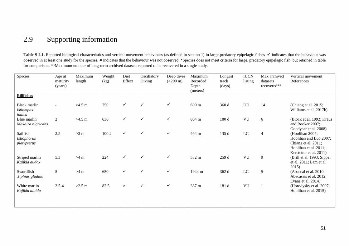
51
2.9 Supporting information
Table S 2.1. Reported biological characteristics and vertical movement behaviours (as defined in section 1) in large predatory epipelagic fishes. indicates that the behaviour was
observed in at least one study for the species, indicates that the behaviour was not observed. *Species does not meet criteria for large, predatory epipelagic fish, but retained in table
for comparison. **Maximum number of long-term archived datasets reported to be recovered in a single study.
Species Age at
maturity
(years)
Maximum
length
Weight
(kg)
Diel
Effect
Oscillatory
Diving
Deep dives
(>200 m)
Maximum
Recorded
Depth
(meters)
Longest
track
(days)
IUCN
listing
Max archived
datasets
recovered**
Vertical movement
References
Billfishes
Black marlin
Istiompax
indica
- >4.5 m 750 600 m 360 d DD 14 (Chiang et al. 2015;
Williams et al. 2017b)
Blue marlin
Makaira nigricans
2 >4.5 m 636 804 m 180 d VU 6 (Block et al. 1992; Kraus
and Rooker 2007;
Goodyear et al. 2008)
Sailfish
Istiophorus
platypterus
2.5 >3 m 100.2 464 m 135 d LC 4 (Hoolihan 2005;
Hoolihan and Luo 2007;
Chiang et al. 2011;
Hoolihan et al. 2011;
Kerstetter et al. 2011)
Striped marlin
Kajikia audax
5.3 >4 m 224 532 m 259 d VU 9 (Brill et al. 1993; Sippel
et al. 2011; Lam et al.
2015)
Swordfish
Xiphias gladius
5 >4 m 650 1944 m 362 d LC 5 (Abascal et al. 2010;
Abecassis et al. 2012;
Evans et al. 2014)
White marlin
Kajikia albida
2.5-4 >2.5 m 82.5 387 m 181 d VU 1 (Horodysky et al. 2007;
Hoolihan et al. 2015)
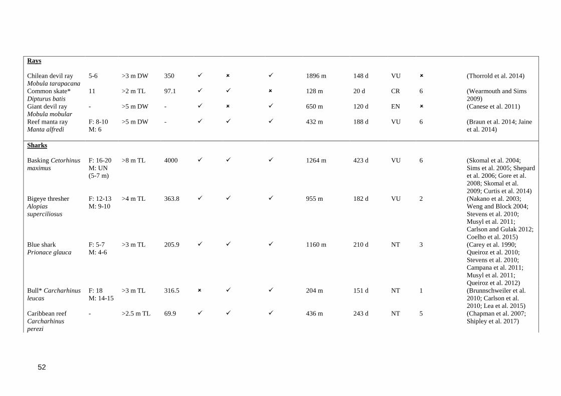
52
Rays
Chilean devil ray
Mobula tarapacana
5-6 >3 m DW 350 1896 m 148 d VU (Thorrold et al. 2014)
Common skate*
Dipturus batis
11 >2 m TL 97.1 128 m 20 d CR 6 (Wearmouth and Sims
2009)
Giant devil ray
Mobula mobular
- >5 m DW - 650 m 120 d EN (Canese et al. 2011)
Reef manta ray
Manta alfredi
F: 8-10
M: 6
>5 m DW - 432 m 188 d VU 6 (Braun et al. 2014; Jaine
et al. 2014)
Sharks
Basking Cetorhinus
maximus
F: 16-20
M: UN
(5-7 m)
>8 m TL 4000 1264 m 423 d VU 6 (Skomal et al. 2004;
Sims et al. 2005; Shepard
et al. 2006; Gore et al.
2008; Skomal et al.
2009; Curtis et al. 2014)
Bigeye thresher
Alopias
superciliosus
F: 12-13
M: 9-10
>4 m TL 363.8 955 m 182 d VU 2 (Nakano et al. 2003;
Weng and Block 2004;
Stevens et al. 2010;
Musyl et al. 2011;
Carlson and Gulak 2012;
Coelho et al. 2015)
Blue shark
Prionace glauca
F: 5-7
M: 4-6
>3 m TL 205.9 1160 m 210 d NT 3 (Carey et al. 1990;
Queiroz et al. 2010;
Stevens et al. 2010;
Campana et al. 2011;
Musyl et al. 2011;
Queiroz et al. 2012)
Bull* Carcharhinus
leucas
F: 18
M: 14-15
>3 m TL 316.5 204 m 151 d NT 1 (Brunnschweiler et al.
2010; Carlson et al.
2010; Lea et al. 2015)
Caribbean reef
Carcharhinus
perezi
- >2.5 m TL 69.9 436 m 243 d NT 5 (Chapman et al. 2007;
Shipley et al. 2017)

53
Common thresher
Alopias vulpinus
F: 3-9
M: 3-7
>4 m TL 348 640 m 177 d VU 4 (Cartamil et al. 2010;
Stevens et al. 2010;
Cartamil et al. 2011)
Dusky shark
Carcharhinus
obscurus
F: 20-21
M: 19
>3 m TL 346.5 573 m 182 d VU 2 (Carlson and Gulak
2012; Rogers et al. 2013;
Hoffmayer et al. 2014)
Galapagos
Carcharhinus
galapagensis
F: 6.5-9
M: 6-8
>3 m TL 85.5 680 m 413 d NT (Meyer et al. 2010;
Papastamatiou et al.
2015a)
Greenland*
Somniosus
microcephalus
- >6 m 775 1560 m 196 d NT (Stokesbury et al. 2005;
Fisk et al. 2012;
Watanabe et al. 2012)
Megamouth
Megachasma
pelagios
- >5.5 m 1327.7 166 m 2 d LC (Nelson et al. 1997)
Oceanic whitetip
Carcharhinus
longimanus
4-5 >3.5 m 167.4 1190 m 335 d VU 16 (Musyl et al. 2011;
Carlson and Gulak 2012;
Howey-Jordan et al.
2013; Howey et al. 2016;
Andrzejaczek et al.
2018)
Pacific sleeper*
Somniosus pacificus
- >4 m 701.3 724 m 336 d DD 3 (Hulbert et al. 2006)
Porbeagle
Lamna nasus
F: 13
M: 8
>3.5 m 230 1600 m 365 d VU 3 (Pade et al. 2009;
Saunders et al. 2011;
Francis et al. 2015; Biais
et al. 2017)
Salmon
Lamna ditropis
F: 6-10
M: 3-5
>3 m 175 1864 m 1168 d LC 11 (Weng et al. 2005;
Carlisle et al. 2011;
Coffey et al. 2017)
Sandbar
Carcharhinus
plumbeus
F: 10-16
M: 8-14
>2 m 117.9 298 m 60 d VU 2 (Barnes et al. 2016)
Scalloped
hammerhead
Sphyrna lewini
F: 4.1-15
M: 3.8-
10
>3 m 152.4 1000m 182 d EN (Klimley 1993;
Jorgensen et al. 2009a;
Bessudo et al. 2011;
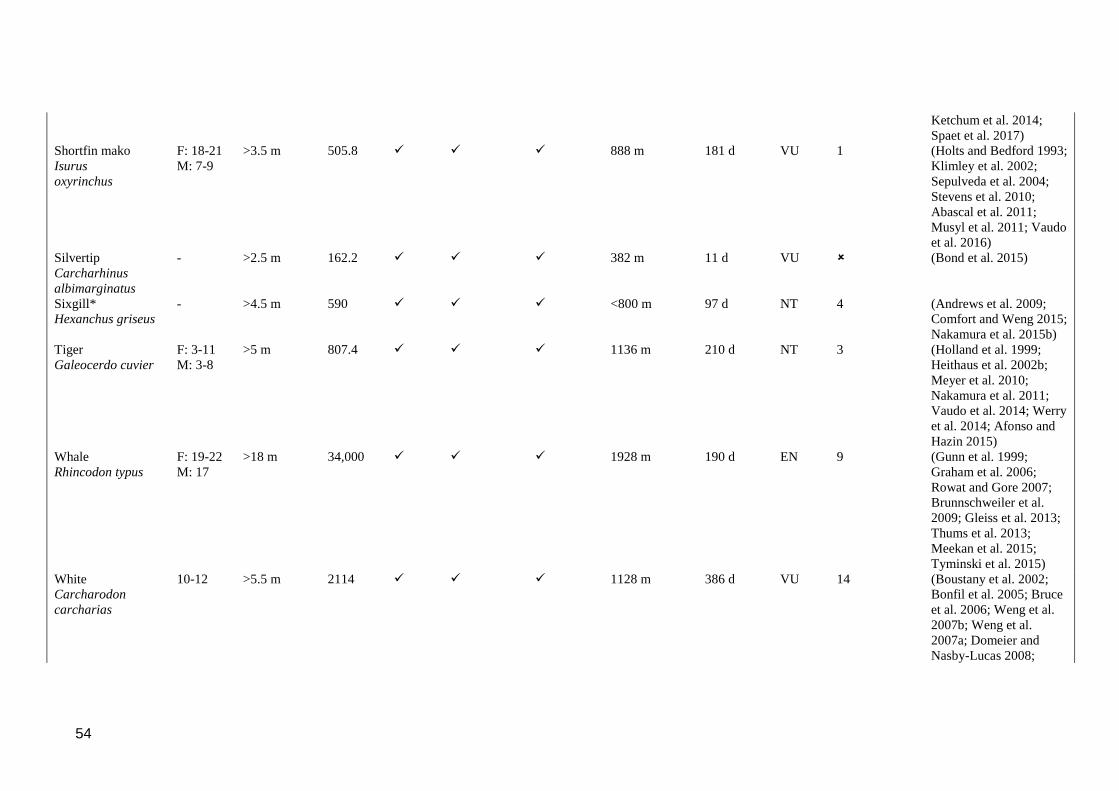
54
Ketchum et al. 2014;
Spaet et al. 2017)
Shortfin mako
Isurus
oxyrinchus
F: 18-21
M: 7-9
>3.5 m 505.8 888 m 181 d VU 1 (Holts and Bedford 1993;
Klimley et al. 2002;
Sepulveda et al. 2004;
Stevens et al. 2010;
Abascal et al. 2011;
Musyl et al. 2011; Vaudo
et al. 2016)
Silvertip
Carcharhinus
albimarginatus
- >2.5 m 162.2 382 m 11 d VU (Bond et al. 2015)
Sixgill*
Hexanchus griseus
- >4.5 m 590 <800 m 97 d NT 4 (Andrews et al. 2009;
Comfort and Weng 2015;
Nakamura et al. 2015b)
Tiger
Galeocerdo cuvier
F: 3-11
M: 3-8
>5 m 807.4 1136 m 210 d NT 3 (Holland et al. 1999;
Heithaus et al. 2002b;
Meyer et al. 2010;
Nakamura et al. 2011;
Vaudo et al. 2014; Werry
et al. 2014; Afonso and
Hazin 2015)
Whale
Rhincodon typus
F: 19-22
M: 17
>18 m 34,000 1928 m 190 d EN 9 (Gunn et al. 1999;
Graham et al. 2006;
Rowat and Gore 2007;
Brunnschweiler et al.
2009; Gleiss et al. 2013;
Thums et al. 2013;
Meekan et al. 2015;
Tyminski et al. 2015)
White
Carcharodon
carcharias
10-12 >5.5 m 2114 1128 m 386 d VU 14 (Boustany et al. 2002;
Bonfil et al. 2005; Bruce
et al. 2006; Weng et al.
2007b; Weng et al.
2007a; Domeier and
Nasby-Lucas 2008;
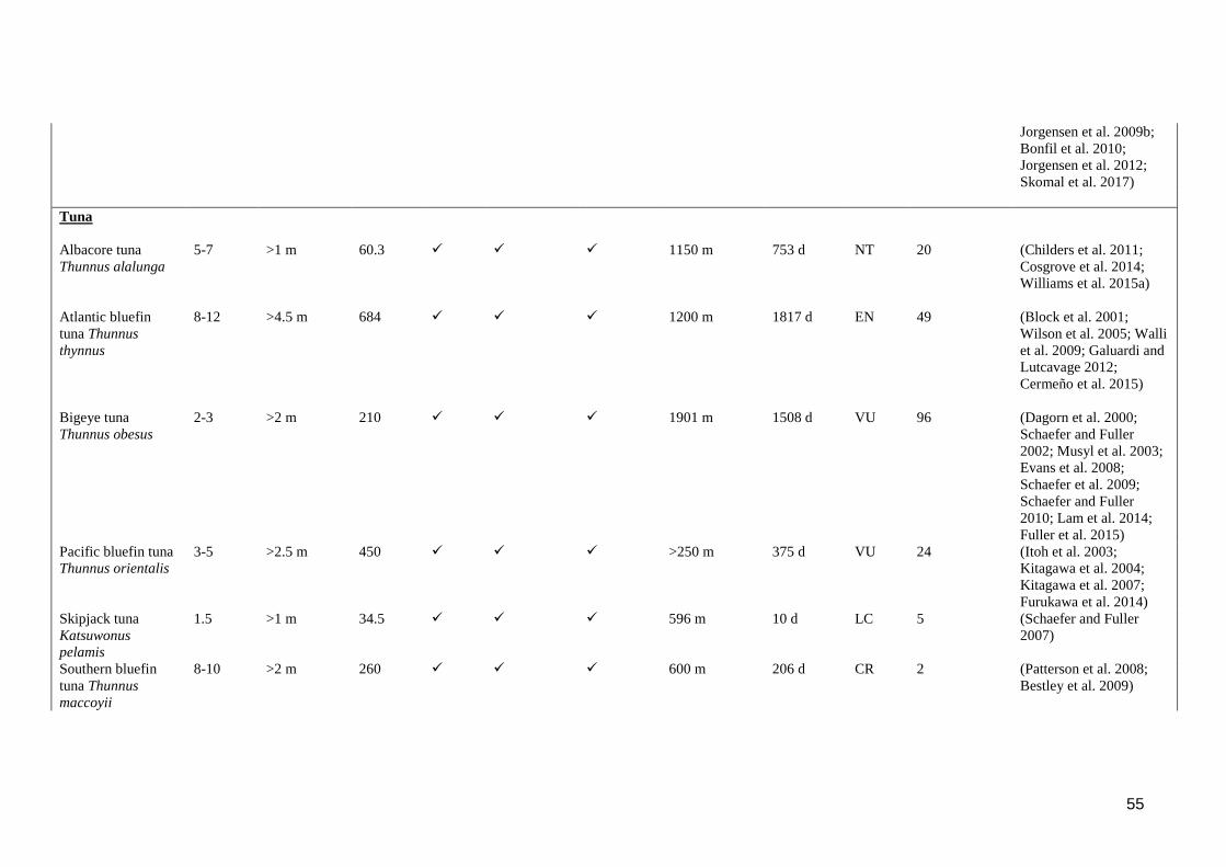
55
Jorgensen et al. 2009b;
Bonfil et al. 2010;
Jorgensen et al. 2012;
Skomal et al. 2017)
Tuna
Albacore tuna
Thunnus alalunga
5-7 >1 m 60.3 1150 m 753 d NT 20 (Childers et al. 2011;
Cosgrove et al. 2014;
Williams et al. 2015a)
Atlantic bluefin
tuna Thunnus
thynnus
8-12 >4.5 m 684 1200 m 1817 d EN 49 (Block et al. 2001;
Wilson et al. 2005; Walli
et al. 2009; Galuardi and
Lutcavage 2012;
Cermeño et al. 2015)
Bigeye tuna
Thunnus obesus
2-3 >2 m 210 1901 m 1508 d VU 96 (Dagorn et al. 2000;
Schaefer and Fuller
2002; Musyl et al. 2003;
Evans et al. 2008;
Schaefer et al. 2009;
Schaefer and Fuller
2010; Lam et al. 2014;
Fuller et al. 2015)
Pacific bluefin tuna
Thunnus orientalis
3-5 >2.5 m 450 >250 m 375 d VU 24 (Itoh et al. 2003;
Kitagawa et al. 2004;
Kitagawa et al. 2007;
Furukawa et al. 2014)
Skipjack tuna
Katsuwonus
pelamis
1.5 >1 m 34.5 596 m 10 d LC 5 (Schaefer and Fuller
2007)
Southern bluefin
tuna Thunnus
maccoyii
8-10 >2 m 260 600 m 206 d CR 2 (Patterson et al. 2008;
Bestley et al. 2009)

56
Yellowfin tuna
Thunnus albacares
1-2 >2 m 200 1602 m 655 d NT 52 (Block et al. 1997;
Schaefer et al. 2009;
Hoolihan et al. 2014;
Schaefer et al. 2014)
Other large
epipelagic
predatory fishes
Dolphinfish
Coryphaena
hippurus
<1 >1.5 m 40 256 m 30 d LC (Furukawa et al. 2011;
Merten et al. 2014)
Oceanic Sunfish
Mola mola
5-7** >3 m 2300 704 m 279 d VU 1 (Cartamil and Lowe
2004; Hays et al. 2009;
Sims et al. 2009; Dewar
et al. 2010; Nakamura et
al. 2015a; Sousa et al.
2016)
Opah Lampris
guttatus
- >2 m 270 736 m 168 d LC (Polovina et al. 2008)
Wahoo
Acanthocybium
solandri
1-2 >2 m 83 296 m 111 d LC 22 (Sepulveda et al. 2011;
Theisen and Baldwin
2012)

57
Chapter 3 Temperature and the vertical
movements of oceanic whitetip
sharks Carcharhinus longimanus
3.1 Abstract
Large-bodied pelagic ectotherms such as sharks need to maintain internal temperatures within a
favourable range in order to maximise performance and be cost-efficient foragers. This implies
that behavioural thermoregulation should be a key feature of the movements of these animals,
although field evidence is limited. We used depth and temperature archives from pop-up satellite
tags to investigate the role of temperature in driving vertical movements of 16 oceanic whitetip
sharks (Carcharhinus longimanus; OWTs). Spectral analysis, linear mixed modelling, segmented
regression and multivariate techniques were used to examine the effect of mean sea surface
temperature (SST) and mixed layer depth on vertical movements. OWTs continually oscillated
throughout the upper 200 m of the water column. In summer, when the water column was
stratified with high SSTs, oscillations increased in amplitude and cycle length and sharks reduced
the time spent in the upper 50 m. In winter, when the water column was cooler and well-mixed,
oscillations decreased in amplitude and cycle length and sharks frequently occupied the upper 50
m. SSTs of 28°C marked a distinct change in vertical movements and the onset of
thermoregulation strategies. Our results have implications for the ecology of these animals in a
warming ocean.
3.2 Introduction
Knowledge of how animals respond to the physical environment is vital for management
strategies and prediction of how climate change will impact their ecology (Schlaff et al. 2014).
Water temperature is arguably the most influential physical driver governing the movements of
marine animals, particularly for ectotherms that cannot internally regulate their body temperature
(Angilletta et al. 2002). As all major physiological processes are sensitive to changes in body
temperature, the physiological performance of ectotherms is directly related to the temperature of
the external environment (Angilletta et al. 2002). Thus, in order to maximize performance, these
animals must use behavioural strategies to thermoregulate by moving through their habitat in a
manner as to maintain optimal body temperatures whenever possible (Neill 1979).
Thermal performance curves (Huey and Stevenson 1979) provide a theoretical basis for an
understanding of this behaviour. These curves describe how body temperature influences
physiological performance and are bounded by the minimum and maximum critical temperatures

58
at which an organism can survive, and the temperatures at which performance is optimized
(Figure 3.1a). The curve is typically skewed so that performance gradually rises from a critical
minimum temperature up to an optimum, before sharply dropping to a critical maximum. As a
result, physiological performance is impacted more by an increase in temperature above optimum
than by an equivalent decrease in temperature below optimum (Martin and Huey 2008). For
terrestrial ectotherms, a global analysis has shown that the primary thermal challenge is to avoid
overheating, especially in tropical and desert areas (Kearney et al. 2009). For this reason,
description of behavioural strategies used as a response to temperature is particularly important
in the context of warming global climate (Kearney et al. 2009).
Sharks and other pelagic fishes that inhabit epipelagic tropical environments could be considered
to be the marine counterparts of these terrestrial ectotherms. Similar to deserts, tropical waters are
warm and have low rates of primary production, so that these marine predators have high
metabolic rates that must be maintained within an oligotrophic ecosystem where prey is sparsely
distributed. In order to survive in these environments, ectotherms need to be cost-efficient
foragers (Gleiss et al. 2011b; Meekan et al. 2015) and must keep their body temperature within
an optimal range. Large marine ectotherms are therefore likely to utilise movements throughout
the water column in order to maintain a thermal range within the bounds required for survival
(Figure 3.1a). Given the typical shape of thermal performance curves, we predict that these
movements will be most critical near the upper temperature limits, where sharp breakpoints in
vertical movement behaviours may become evident as animals seek to maintain body
temperatures below critical values.
Satellite tagging offers a methodology to investigate vertical behaviours by simultaneously
recording depth and ambient temperature. However, transmissions via satellite are typically
restricted to summarised forms. The detailed patterns of vertical movement necessary to
reconstruct relationships between temperature and depth generally require physical recovery of
the tag, in order to access the high-frequency data stored in the tag’s archive. Although this is a
rare event (Stevens et al. 2010; Jorgensen et al. 2012) due to the unpredictability of movements
post-tagging and the open ocean environments inhabited by pelagic sharks, such tags are
occasionally recovered and provide access to data that is sampled at sufficient temporal scales to
investigate hypotheses concerning the drivers of movement patterns (Howey et al. 2016).
Oceanic whitetip sharks (Carcharhinus longimanus; OWTs) are large, epipelagic, predatory
ectotherms (maximum body mass >150 kg; Froese and Pauly 2017)) that are globally distributed
in warm-temperate and tropical oceans (Bonfil et al. 2008). Here, we analyse high-resolution data
archived from 16 recovered tags deployed on OWTs in the western North Atlantic Ocean for a
mean of 183 ± 91 days. These data are used to test the hypothesis that, in a seasonally changing
water column, OWTs will change their vertical movement patterns to avoid prolonged exposure

59
to the highest SSTs. Given the shape of the typical thermal performance curve, we predict a
distinct upper temperature breakpoint in vertical behaviour. Further, we characterise the
behaviours that these sharks use to maintain body temperature, and discuss the likely drivers of
individual variation in these behaviours.
Figure 3.1. Schematic diagrams of (a) hypothetical performance curve of an ectotherm adapted from Huey
and Stevenson (1979). The curve describes the temperature for which performance is optimised (Topt) and
the critical minimum and maximum temperatures (Tcritmin and Tcritmax) at which an organism can survive;
and (b) the cyclic characteristics of oscillatory movements; mean cycle length and cycle amplitude were
extracted from a continuous wavelet transformation on depth data.
3.3 Materials and methods
3.3.1 Data collection
Oceanic whitetip sharks were captured and tagged with Standard Rate (SR) X-Tags (Microwave
Telemetry, Inc., Columbia, MD) near Cat Island, The Bahamas (24.12°N, 75.28°W) during May
2011-2013. All equipment, tagging procedures and analysis of horizontal data are described in
detail elsewhere (Howey-Jordan et al. 2013; Howey et al. 2016). In brief, a handheld tagging
applicator was used to insert X-Tags into the dorsal musculature of captured sharks. These tags
recorded depth (0.34 m resolution), temperature (0.16-0.23°C resolution), and light levels at two-
minute intervals. Physical recovery of the tags allowed for whole archival datasets to be
downloaded. This sampling frequency was assessed to adequately capture the vertical movements
of these sharks by comparing profiles obtained at one-second intervals with a two-minute
subsample recorded by an individual tagged with a PD3GT data logger (1 Hz, ± 0.25 m resolution)
(Little Leonardo, Tokyo, Japan; Watanabe et al. 2015; Howey et al. 2016). Prior to analysis, the
first and last day of the tag deployment was discarded from each dataset.
Research was conducted under the Cape Eleuthera Institute (CEI) research permit (MAF/FIS/17
& MAF/FIS/ 34) issued by the Bahamian Department of Marine Resources in accordance with

60
CEI animal care protocols developed within the guidelines of the Association for the Study of
Animal Behaviour and the Animal Behaviour Society.
3.3.2 Data analysis
We used R 3.4.0 for all data analysis (R Core Team 2017), except where stated otherwise.
3.3.2.1 Environmental parameters
Daily mean sea surface temperatures (SST) and mixed layer depths (MLD) were calculated using
depth and temperature data collected by tagged individuals. SST was calculated as the mean
temperature in the uppermost 5 m of the water column each day. MLD was calculated using the
threshold method (de Boyer Montégut et al. 2004). We chose this approach as the tags did not
record salinity, preventing us from using density criteria, and the sampling interval prevented the
sharp gradient-resolved profiles required for gradient criterion (de Boyer Montégut et al. 2004).
The threshold method involves determining the depth at which there was a change in temperature
from a near-surface reference depth by more than a chosen threshold value. The daily mean
temperature from the 7.5-12.5 m depth bin was used as a reference value to avoid the diurnal
variation in the surface layer (de Boyer Montégut et al. 2004) and a classical threshold value of
0.5°C (Levitus 1982) was selected based on visual inspection of daily temperature-depth profiles
recorded by the tags.
3.3.2.2 Vertical movement behaviours
The cyclic nature and amplitude of vertical movements were analysed using the software Igor Pro
(WaveMetrics Inc., Lake Oswego, OR, USA) with the package Ethographer (Sakamoto et al.
2009). Continuous wavelet transformation was applied to the entire depth dataset of each shark.
Based on visual inspection of the depth profiles, minimum and maximum cycle length in
Ethographer were set to 10 minutes and 90 minutes, respectively. The mean cycle length
(seconds) and amplitude (meters) (see Figure 3.1b) of these cycles were extracted and a daily
mean was calculated.
For each day, mean depth and temperature, the mean time spent outside of the mixed layer and
the proportion of time spent within distinct depth ranges were also calculated. Preliminary
analysis revealed that the proportion of time spent in the top 50 m displayed the strongest
relationship with environmental parameters. For this reason, this depth range was used for further
analyses.
3.3.2.3 Generalised linear mixed models
We built three generalised linear mixed models (GLMMs) using the nlme (Pinheiro et al. 2017)
package in R to investigate relationships among daily means of environmental parameters,
61
vertical distribution and oscillatory behaviour. The explanatory variables for each model were
initially set as SST, MLD and total length of the shark (hereafter length), and shark identity as a
random variable. Mean depth, proportion of time in the upper 50 m and mean cycle length were
all sequentially modelled as response variables. The proportion of time spent in the top 50 m was
logit transformed prior to analysis. We used the corAR1 function to account for temporal auto-
correlation in our datasets (Zuur et al. 2009). All possible combinations of the explanatory
variables were modelled, and resulting models were compared and ranked using weights of
Akaike’s information criterion (AIC).
3.3.2.4 Breakpoint analysis
Potential breakpoints in the relationships between SST and vertical movement behaviours were
initially identified through visual inspection. Breakpoints occur where there is a sudden and sharp
change in the directionality of a linear relationship. Piecewise regression was used to statistically
estimate these breakpoints by fitting separate slopes for data above and below modelled
breakpoints until the best fit was found. This method has traditionally been used to successfully
estimate breakpoint positions and ecological thresholds in species-habitat relationships in the
terrestrial realm (Francesco Ficetola and Denoël 2009), and has more recently been applied in
predicting optimal temperatures for the activity of ectothermic fishes such as Arctic char,
Salvelinus alpinus (Hansen et al. 2017). We used an iterative searching method with SST set as
the explanatory variable, and mean cycle length and proportion of time spent in the upper 50 m
each set in turn as the dependent variable. Each unique SST was used as a breakpoint and a linear
regression was run for all possible breakpoints. The model with the lowest residual mean squared
error (MSE) was used to select the breakpoint. The AIC of models with and without the breakpoint
term were compared for the full dataset as well as for each individual shark.
3.3.2.5 Multivariate analysis – hierarchical clustering
Where distinct breakpoints in vertical movement behaviours in response to SST were found, we
applied a hierarchical cluster analysis to categorise vertical behaviours employed in the upper
thermal range. This method has been used by earlier studies to successfully distinguish among
behavioural modes of vertical movement in marine megafauna (Jorgensen et al. 2012; Thums et
al. 2013). The proportion of time spent in the top 50 m, mean depth, mean cycle length and mean
amplitude were summarised to daily values and scaled using the scale function in R. Cluster
analysis was applied on these variables using the hclust function in R based on a dissimilarity
matrix produced from Euclidean distances and complete linkage as the agglomeration method.
We then used principal components analysis (PCA) on these clustered data to determine if vertical
movement behaviours differed among the resulting groups. Vertical movement behaviours were
then examined by clusters and were subjectively broken into groups based on the distance
between clusters and the cluster characteristics. Sharks with less than 50 days of data within the

62
given SST range were not included in this analysis. To determine which individuals were most
similarly grouped, the same clustering procedure was used on the proportion of time spent in each
cluster.
3.4 Results
3.4.1 Track summary
Sixteen X-Tags were recovered from mature sharks providing access to 183 ± 91 days (mean ±
standard deviation) of tracking data with a range of 20-333 days (see Table S 3.1 for more detailed
deployment information). Individuals spent 99.64 ± 1.15% time in the upper 200 m of the water
column, with a principal part of this time in the upper 100 m (90.10 ± 13.08%, Figure 3.2a).
Mesopelagic Excursions (>200 m depths) occurred throughout the year (see Howey et al. 2011
for detailed analyses of these movements). Over the year the mixed layer depth (MLD) increased
from a depth of 28.07 ± 10.11 m in summer (21st June – 22nd September) to 64.85 ± 24.93 m in
winter (21st December – 20th March) as the water column became increasingly well-mixed. Daily
mean sea surface temperature (SST) decreased from 28.55 ± 0.81°C during the summer months
to 25.59 ± 1.07°C during winter months. The mean temperature range from the sea surface to 100
m depth also decreased from 3.88 ± 0.72°C in summer to 0.99 ± 0.39°C in winter (Figure 3.2).
3.4.2 Oscillatory diving behaviours and environmental
conditions
Tagged OWTs continually descended and ascended through the water column. Continuous
wavelet transformation analysis was used to estimate daily mean cycle length (time to complete
an oscillation) and daily mean amplitude (depth of oscillation) (see Figure 3.1b) of these vertical
movements. Vertical distribution and cyclic characteristics changed with environmental
conditions (Figure 3.1b, Figure 3.3). An initial visual inspection of the depth profile indicated that
most time was spent in the top 50 m of the water column, especially in winter months when it was
cooler with larger vertical mixing (Figure 3.3a, Figure 3.3c). As the SST increased in summer
months, depth profiles displayed avoidance of the surface 50 m where waters were warmest
(Figure 3.3b) or larger and longer cycle oscillations (Figure 3.3d).
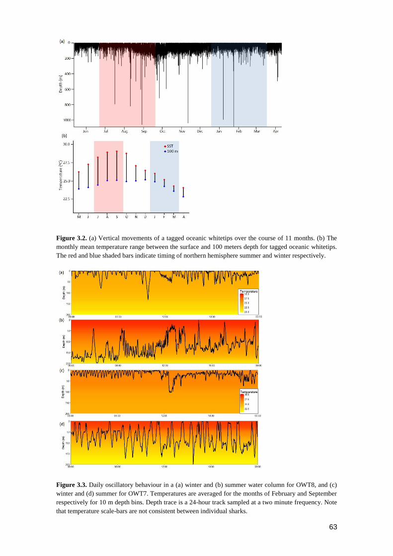
63
Figure 3.2. (a) Vertical movements of a tagged oceanic whitetips over the course of 11 months. (b) The
monthly mean temperature range between the surface and 100 meters depth for tagged oceanic whitetips.
The red and blue shaded bars indicate timing of northern hemisphere summer and winter respectively.
Figure 3.3. Daily oscillatory behaviour in a (a) winter and (b) summer water column for OWT8, and (c)
winter and (d) summer for OWT7. Temperatures are averaged for the months of February and September
respectively for 10 m depth bins. Depth trace is a 24-hour track sampled at a two minute frequency. Note
that temperature scale-bars are not consistent between individual sharks.

64
Three generalised linear mixed models were built to investigate relationships among daily means
of environmental parameters, vertical distribution and oscillatory behaviour. All three models
retained SST and MLD as explanatory variables and removed animal length in the model selection
process (Table 3-1). A total of 35% of the variation in mean daily depth was explained by our
first model with 21% attributed to variation in SST. Mean daily depth increased with SST,
attaining a mean of 33.68 ± 15.83 m in winter and 56.50 ± 20.02 m in summer. Our second model
explained 47% of the variation in the daily proportion of time spent in the top 50 m, with SST
accounting for 31% of this variation (Table 3-1). The proportion of time spent in the top 50 m
displayed a negative relationship with SST (Figure 3.4a). Although model selection retained SST
and MLD as explanatory variables of mean cycle length, these parameters did not explain a
substantial proportion of the variation (Table 3-1). For all three models, conditional R2 values and
individual OWT plots suggest high inter-individual variability in vertical movement behaviours
(see Figure S 3-1).
Table 3-1. Subset of model comparisons using Akaike's Information Criterion (AIC), Bayesian Information
Criterion (BIC) and conditional (R2c) and marginal (R2m) R2 values. ΔAIC displays deviance in AIC scores
from top-ranked models. All models are generalised linear mixed models and were ran using the nlme
package in R with shark identity as a random variable. Proportion of time spent in the top 50 m (Prop50)
was logit transformed prior to analysis. All null models include the random effect. To see all models
involved in the model selection process, see Table S 3.2.
Model DF AIC BIC ΔAIC wAIC R2c R2m
1. Mean depth ~ SST + MLD 2839 21634 21682
0.645 0.35 0.23
Mean depth ~ SST + MLD + Length 2839 21636 21689 2 0.355 0.35 0.24
Mean depth ~ SST 2840 21671 21713 37 0.00 0.33 0.21
Mean depth ~ 1 2841 21693 21729 59 0.00 0.32 0
2. Prop50 ~ SST + MLD 2839 7104 7152
0.664 0.46 0.32
Prop50 ~ SST + MLD+ Length 2839 7106 7159 2 0.336 0.46 0.33
Prop50~ SST 2840 7140 7182 36 0.00 0.46 0.31
Prop50~ 1 2841 7170 7206 47 0.00 0.62 0
3. Mean cycle length ~ SST + MLD 2839 43765 43812
0.668 0.43 0.05
Mean cycle length ~ SST + MLD + Length 2839 43767 43820 2 0.246 0.43 0.05
Mean cycle length ~ SST 2840 43814 43856 49 0.00 0.40 0.03
Mean cycle length ~ 1 2841 43818 43854 53 0.00 0.41 0

65
Figure 3.4. Relationship between SST and (a) daily % of time spent in the top 50 m and (b) daily mean
cycle length (s). Red and blue lines display results of piecewise regression with the blue line indicating the
breakpoint, and the red lines the linear relationship either side of this breakpoint.
3.4.3 Vertical behavioural breakpoints
A breakpoint of approximately 28°C occurred in the relationships of both daily proportion of time
spent in the top 50 m and mean cycle length with SST (Figure 3.4). Above 27.8°C, the weak
negative relationship between mean SST and proportion of time spent in the top 50 m steepened
considerably from a slope of -2.86 to -13.99 (Figure 3.4a). The mean proportion of time spent in
the top 50 m of the water column at SSTs above and below 27.8°C was 38.21 ± 19.44% and 71.15
± 20.24% respectively. Beyond this breakpoint, individuals rarely spent more than 80% of their
time in the top 50 m. Below a 28.2°C breakpoint, there was no apparent relationship between
mean cycle length and SST (Figure 3.4b). For days exceeding this breakpoint, a positive
relationship with a slope of approximately 329 s was found. Mean cycle length increased from
2570 ± 793 s when SST was below 28.2°C to 3060 ± 677 s when SST was above 28.2°C. Mean
values for other vertical movement parameters above and below an estimated 28°C breakpoint
are listed in Table 3-2. Notably, mean SST increased by more than two degrees between these
two groups, however the overall mean temperature experienced by tagged sharks increased by
less than one degree. The inclusion of the breakpoint term minimised the AIC for both full models,
however, the result was more variable when assessed on an individual basis (Table S 3.3, Table
S 3.4). The AIC suggested that in 11 of 13 individuals the inclusion of a breakpoint between 27-
29°C had greater support than a single linear relationship (ΔAIC = 6-122) for the daily proportion
of time spent in the top 50 m, and nine individuals the inclusion of the breakpoint for mean cycle
length had greater support than the single linear relationship (ΔAIC = 6-60).

66
Table 3-2. Mean (± standard deviation) of daily vertical movement behaviours above and below 28°C.
Parameter Below 28oC Above 28oC
Mean SST 26.56 ± 0.96oC 28.91 ± 0.48oC
Mean temperature 25.70 ± 0.83oC 26.66 ± 0.79oC
Mean depth 38.63 ± 17.0 m 63.06 ± 18.20 m
% time spent in top 50 m 70.61 ± 20.41% 37.57 ± 19.17%
Mean cycle length of oscillations 2576 ± 788 s 3013 ± 711 s
Mean amplitude of oscillations 14.76 ± 6.25 m 20.74 ± 8.0 m
Mean MLD 39.20 ± 23.36 m 32.01 ± 10.65 m
3.4.4 Cluster analysis
To further classify vertical movements when surface waters warmed, metrics of vertical
movement including mean depth, proportion of time spent in the top 50 m, mean cycle length and
mean amplitude were used for a hierarchical cluster analysis for individual days when the SST
exceeded 28°C. Three individual OWTs were excluded due to an insufficient sample size of days
meeting this criteria (<50 days). Six clusters emerged from this analysis and the PCA indicated
that 77.6% of the variation in these vertical movement behaviour could be explained by the first
two components (Figure 3.5). The proportion of time spent at depths <50 m and mean daily depth
each contributed to more than 40% of the variation in PC1, and mean daily cycle length and mean
daily amplitude each contributed to more than 35% of the variation in PC2. Characteristics of
each cluster are summarised in Table 3-3, and a representative example of each are displayed in
Figure 3.6. Cluster 4 was the most common (37.21% of days) and was characterised by a low
proportion of time spent in the top 50 m and short cycle (approximately 44 minutes) and low
amplitude oscillations (Table 3-3). Cluster 1 was the second most common (27.83%) and showed
medium levels of both time spent in the top 50 m and cycle length. Clusters 2 and 3 both showed
long cycles of approximately one hour with cluster 2 being distinguished by very low use of the
top 50 m of the water column. Cluster 5 was characterised by higher use of the top 50 m and
oscillations with relatively small amplitude and short cycles. Although the proportion of the time
spent within the top 50 m for sharks within this cluster was high, the mean MLD was relatively
shallow and the mean time spent outside the ML was comparable with other clusters (Table 3-1).
Cluster 6 only comprised 0.93% of the data, and was characterised by oscillations with the longest
cycle and highest amplitude. Days associated with this cluster were found to have repeated deep
descents to depths greater than 200 m (Figure 3.6f). In summary, the clusters were composed of
different combinations of vertical behaviours that collectively avoided prolonged exposure to the
warmest temperatures found in the surface layers. In addition, with the exception of Cluster 1, the
mean daily temperature was maintained within a standard deviation of the overall mean daily
temperature recorded by the tags (26.14 ± 0.94°C).

67
Figure 3.5. Results from multivariate analysis of daily data where SST >28°C. Input variables were daily
values of proportion of time spent in the top 50 m, mean depth, mean cycle length and mean amplitude. (a)
Dendrogram of vertical movement behaviour determined from hierarchical cluster analysis. (b) The two
principal components scores are plotted for daily data. Points are coloured by their cluster group.
Table 3-3. Summarised characteristics of each cluster derived from the hierarchical cluster analysis. Values
are mean ± standard deviation.
Cluster ID 1 2 3 4 5 6
% days 27.83% 15.12% 12.17% 37.21% 6.74% 0.93%
Mean % time
top 50
51.72 ±
12.44%
17.18 ±
7.69%
45.13 ±
13.17%
25.98 ±
9.07%
67.78 ±
14.22%
40.68 ±
10.64%
Mean depth 50.42 ± 11.99
m
82.43 ± 13.04
m
64.41 ± 17.85
m
68.90 ± 10.60
m
38.41 ± 10.95
m
95.32 ± 25.22
m
Mean cycle
length
3168 ± 509 s 3651 ± 390 s 3620 ± 410 s 2637 ± 528 s 1914 ± 642 s 3995 ± 357 s
Mean
amplitude
19.82 ± 4.72
m
17.51 ± 4.59
m
33.02 ± 6.81
m
19.01 ± 4.81
m
14.43 ± 3.64
m
60.91 ± 8.50
m
Mean
temperature
27.13 ±
0.64oC
26.53 ±
0.65oC
26.57 ±
0.82oC
26.41 ±
0.70oC
26.72 ±
1.11oC
25.73 ±
0.81oC
Mean MLD 31.77 ± 11.37
m
39.68 ± 10.28
m
30.39 ± 9.62
m
32.15 ± 8.55
m
20.84 ± 7.11
m
33.88 ± 8.34
m
Mean % time
outside ML
63.48 ±
15.81%
86.98 ±
7.22%
64.30 ±
14.44%
84.66 ±
8.81%
67.54 ±
22.44%
63.26 ±
10.36%
Mean SST 28.84 ±
0.49oC
29.21 ±
0.43oC
28.91 ±
0.42oC
28.93 ±
0.44oC
28.58 ±
0.46oC
29.28 ±
0.22oC
Behaviour Medium %
top 50,
medium
cycles, low
amplitude
Low % top
50, long
cycles, low
amplitude
Medium %
top 50, long
cycles,
medium
amplitude
Low % top
50, short
cycles, low
amplitude
High % top
50, short
cycles, low
amplitude
Medium %
top 50, long
cycles, high
amplitude

68
Figure 3.6. 24-hour depth profiles representative of each group derived from the hierarchical cluster
analysis. a) Medium % top 50, medium cycles, low amplitude, b) low % top 50, long cycles, low amplitude,
c) medium % top 50, long cycles, medium amplitude, d) low % top 50, short cycles, low amplitude, e) high
% top 50, short cycles, low amplitude, f) medium % top 50, long cycles, high amplitude. Note that the scale
on the y-axis differs for Cluster 6.
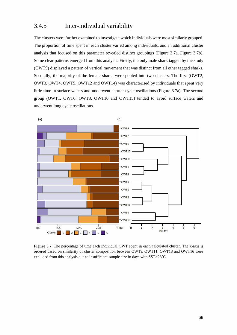
69
3.4.5 Inter-individual variability
The clusters were further examined to investigate which individuals were most similarly grouped.
The proportion of time spent in each cluster varied among individuals, and an additional cluster
analysis that focused on this parameter revealed distinct groupings (Figure 3.7a, Figure 3.7b).
Some clear patterns emerged from this analysis. Firstly, the only male shark tagged by the study
(OWT9) displayed a pattern of vertical movement that was distinct from all other tagged sharks.
Secondly, the majority of the female sharks were pooled into two clusters. The first (OWT2,
OWT3, OWT4, OWT5, OWT12 and OWT14) was characterised by individuals that spent very
little time in surface waters and underwent shorter cycle oscillations (Figure 3.7a). The second
group (OWT1, OWT6, OWT8, OWT10 and OWT15) tended to avoid surface waters and
underwent long cycle oscillations.
Figure 3.7. The percentage of time each individual OWT spent in each calculated cluster. The x-axis is
ordered based on similarity of cluster composition between OWTs. OWT11, OWT13 and OWT16 were
excluded from this analysis due to insufficient sample size in days with SST>28°C.

70
3.5 Discussion
Theories of foraging ecology and thermal physiology suggest that large animals found in tropical
environments should maintain an optimal and stable body temperature range (Huey and
Stevenson 1979; Sims 2003; Bernal et al. 2012). This stability is required because a number of
physiological processes, such as growth, have a tendency to increase with temperature. Thus, an
individual will have optimal performance if temperatures are maintained within the upper limits
of this range, assuming there is sufficient prey available to support the relatively high metabolic
rates that this entails (Hight and Lowe 2007; Bernal et al. 2012; Whitney et al. 2016a). Due to the
asymmetry of the thermal performance curve, slight increases in temperature above optimum can
result in rapid declines in performance (Martin and Huey 2008). This will require aquatic
ectotherms to vacate environments when temperatures become unfavourable for maintaining
performance. We predicted that OWTs would modify their diving behaviour as the thermal
structure of the water column changed seasonally and that sharp behavioural breakpoints would
be evident at higher temperatures that might indicate the upper limits of thermal performance
curves. In cooler months, when SST was lower than 28°C, OWTs spent a high proportion of their
time in the top 50 m of the water column. Beyond this limit, OWTs avoided the top 50 m where
waters were the warmest, and/or performed longer cycle and higher amplitude oscillations from
the surface to deeper, cooler waters. As a result, the mean daily temperature experienced by the
shark shifted by only a degree (25.70 ± 0.83°C below 28°C SST, 26.66 ± 0.79°C above 28°C),
despite much larger changes in SST in the top 50 m of the water column across the season.
Evidence for a behavioural breakpoint with changes in temperature are consistent with the
hypothesis that OWT sharks have behavioural strategies for thermoregulation. Our data suggests
that OWT sharks in the western North Atlantic Ocean face metabolic challenges similar to some
terrestrial ectotherms (Kearney et al. 2009) in having to cope with habitats close to upper thermal
limits and potential overheating. To date, most studies of strategies for thermoregulation in marine
ectotherms have focused on behaviours that might function to regain heat lost after descents into
deeper and cooler waters to feed on the deep scattering layer (Thums et al. 2013; Nakamura et al.
2015a). There is, however, evidence that endothermic fishes that inhabit cooler waters might face
similar physiological challenges when migrating through warmer latitudes. For example, Teo et
al. (2007) hypothesised that Atlantic bluefin tuna (Thunnus thynnus) descended to deeper waters
on entry and exit to the Gulf of Mexico in order to avoid warm surface waters. Similarly, female
porbeagle sharks (Lamna nasus) are thought to avoid warm surface waters (22-29°C) in the Gulf
Stream and Sargasso Sea, with no individual recorded in waters with a six-hour mean greater than
21.9°C (Campana et al. 2011). In the northern Pacific, salmon sharks (L. ditropis) have been found
to descend to deeper, cooler waters as they migrate south towards lower latitudes (Weng et al.
2005; Coffey et al. 2017). Tagged individuals of this species generally positioned themselves at
71
deeper and cooler depths when surface temperatures exceeded 23°C in a multi-year satellite tag
dataset (Coffey et al. 2017). These observations suggest that breakpoints in vertical movement
behaviours at high SSTs might also exist in other species, both endothermic and ectothermic.
Although OWTs displayed a variety of vertical movement behaviours that we suggest avoided
prolonged exposure to surface waters when SST warmed above 28°C, these behaviours were not
necessarily consistent among tagged individuals. Such inter-individual variation has been
reported by many studies tracking both the horizontal and vertical movements of sharks (Musyl
et al. 2011; Vaudo et al. 2014; Ferreira et al. 2015). In our study, the most important differences
in vertical behaviours among OWT sharks occurred in the proportion of time individuals resided
in the top 50 m of the water column and in the length and amplitude of their vertical oscillations,
although it is important to note that despite this variation in strategies, mean water temperatures
experienced by the sharks were always maintained between 25-27°C. Whereas at present we
cannot be certain of the drivers of these individual variations in movement patterns, differences
could reflect the influence of prey availability, ontogenetic and reproductive stage, intraspecific
interactions and interaction with predators, and/or differences in thermal physiology.
Regardless of the use of horizontal space by an individual shark, all OWTs underwent
mesopelagic excursions to depths of up to 1190 m, a behaviour that may represent prey searching
(Howey et al. 2016). Around the tagging locality of Cat Island, OWTs are thought to feed
predominately on large pelagic teleosts and after movement away from this region, their diet alters
to include a significantly higher proportion of squid (Madigan et al. 2015). Such changes in diet
and the consequent distribution of potential prey may drive differences in vertical behaviours
among individuals, by determining whether an individual needs to access warmer surface waters.
If prey are available at depth, an OWT will not need to enter the top 50 m, whereas if prey are
only available in surface waters, an individual may undergo longer oscillations to cooler depths
in order to dissipate excess heat gained while foraging in surface layers. Similarly, individual
dietary specialisation may drive differences in movements if preferred dietary items differ in their
vertical distributions. Comparing the isotopic composition of tagged individuals may help to
assess differences in vertical behaviours.
We tagged sharks at an aggregation site off Cat Island, in the Bahamas. The sex ratio of the
aggregation is dominated by females that either remain in the region year round or undergo long-
distance migrations that commence around July (Howey-Jordan et al. 2013), coinciding with
seasonal warming of surface waters. The onset of changes in vertical habitat use we observed –
higher-amplitude and longer cycle oscillations and avoidance of waters >28°C – were not
confined to those individuals that migrated, since one female shark (OWT3) that remained near
the Bahamas also exhibited the same pattern of avoidance of the upper 50 m depths as surface
waters warmed. In contrast, the only male tagged by our study remained near the Bahamas (except

72
for a three-week period from late August through early September), but did not have any obvious
strategy in vertical movements that avoided the warmest surface waters. While bearing in mind
the limitations of generalisations based on the results from a single tag, it might be possible that
this difference between males and females occurs because females have a greater need to maintain
a narrower thermal range due to higher energetic demands (Schlaff et al. 2014). A larger number
of males need to be sampled to investigate this possibility.
The total length of the tagged individuals did not appear to drive any of the variation in movement
patterns among individuals and, as a majority were mature females, we could not explore the
effect of sex or life history stage in detail. As OWTs are thought to have biennial reproductive
cycles (Tambourgi et al. 2013), it is possible that differences in patterns of vertical movement we
documented among females may arise from reproductive status, as developing pups may make
greater metabolic demands and thus require higher rates of food intake and/or maintenance of
body temperatures within a smaller temperature range.
Our results were consistent with the hypothesis that OWT sharks display behavioural strategies
that maintain stable body temperatures in a warm and oligotrophic tropical environment. An
understanding of relationships between vertical movement behaviours and ambient temperature
is essential if we are to document the capacity for ectothermic sharks to buffer the impact of
changing environmental conditions, particularly warming oceans (Kearney et al. 2009).
Irrespective of SST, sharks experienced very similar mean daily temperatures throughout the time
they were tagged. This was achieved in a variety of ways when waters warmed above 28°C. At
temperatures below this breakpoint, OWTs continually displayed oscillatory diving behaviour,
even when the water column was well-mixed down to 100 m, suggesting that thermoregulation
was not the primary driver of these movements (Figure 3.3a, Figure 3.3c). We also acknowledge
that some other unmeasured environmental variable, such as light or water quality, prompted the
observed changes in vertical movement behaviours. Nevertheless, if this was the case, OWTs
would likely continue to benefit from the maintenance of a stable body temperature.
Although these behaviours demonstrate the potential of OWTs to adapt to a warming ocean, there
are several implications of these results. Given variability in species thermal optima, potential
habitat mismatches between OWT and their prey are possible in the future if warming increases
thermal habitat close to upper thermal limits, reducing the zone of overlap in which OWTs can
feed (Hazen et al. 2013). This avoidance of surface waters will reduce the vulnerability of these
sharks to fishing gears targeting this zone, but may increase their vulnerability to deeper-set
longlines by compressing the zone of available habitat for OWTs (Dulvy et al. 2014), magnifying
the spatial overlap of OWT distributions with pelagic longline fisheries that already occurs on a
horizontal scale (Tolotti et al. 2015a). In winter months, when the top 100 m becomes well-mixed,
these problems may be compounded if winter SSTs begin to attain upper thermal limits and sharks

73
have to descend to greater depths to reach cooler temperatures. Fortunately, in recent years, SSTs
in regions around the Bahamas have followed a cooling trend in winter months (Chollett et al.
2012), however, this may be a problem confronting the species in other regions. Additionally,
other impacts of climate change may also influence the response of OWTs to a warming ocean.
Lower oxygen content of warming waters may reduce the ability of sharks to chase prey (Pistevos
et al. 2016), escalating the difficulties facing OWTs in an oligotrophic pelagic environment.
Several studies have reported declines in the abundance and size of the OWT (Baum and Myers
2004; Cortés et al. 2007; Clarke et al. 2012). Although the retention of OWTs by fisheries has
generally been banned, high spatial overlap with targeted species means capture rates are unlikely
to decline and other strategies are needed to conserve populations (Tolotti et al. 2015b).
Anticipating future seasonal and overall shifts in vertical distribution will have important
implications for developing and implementing effective mitigation measures such as spatial
and/or temporal closures.
In order to measure the impacts of warming on the physiological performance of OWTs, we need
to quantify the upper limits of the thermal performance curve for the species. Traditionally,
respirometry approaches have provided the data on metabolic rate and cost of transport of fishes
under different temperature regimes (Whitney et al. 2016a) , although this usually requires captive
trials in laboratories and are unlikely to be a logistically feasible option. However, accelerometry
now offers a viable technique for calculating the metabolic rate of these animals (Lear et al. 2016)
and deployment of tags containing accelerometers in different seasons to compare energy
expenditure at SSTs above and below 28°C will be crucial for predicting the future consequences
of a warming ocean. It is also vital that we continue to explore how temperature structures the
vertical movements of sharks and incorporate our findings into projections of future distribution
shifts of these animals. As the effect of temperature may vary between regions for a given species,
it will also be useful to assess vertical movements on a broader geographical range.
3.6 Acknowledgements
Michele Thums, Luciana Ferreira and two anonymous reviewers for critical comments that
greatly enhanced the quality of the manuscript.

74
3.7 Supporting information
Table S 3.1. Summary of tagging information and biological information of the tagged individuals.
Shark ID Deployment
date
Days at
liberty
Fork length
(cm)
Sex Pop-off
latitude (oN)
Pop-off
longitude
(oS)
Mean (± SD)
depth (m)
Mean (± SD)
temperature
(oC)
Maximum
depth (m)
Minimum
temperature
(oC)
OWT1 5/1/2011 184 218 F 22.89 74.68 59.92 ± 45.02 26.35 ± 1.68 1081.9 7.75
OWT2 5/4/2011 153 189 F 23.20 74.91 46.02 ± 38.52 26.16 ± 1.87 1008.7 8.54
OWT3 5/4/2011 245 214 F 23.73 74.93 50.03 ± 37.29 26.59 ± 1.46 751.8 10.89
OWT4 5/1/2011 153 233 F 24.36 75.37 41.66 ± 37.42 25.98 ± 1.66 720.2 7.90
OWT5 5/7/2012 245 212 F 24.60 75.50 43.32 ± 33.9 26.18 ± 1.56 577.3 13.53
OWT6 5/7/2012 150 179 F 22.69 73.38 50.8 ± 39.9 27.09 ± 1.65 635.1 11.04
OWT7 5/11/2012 278 228 F 23.94 74.93 45.37 ± 48.83 26.34 ± 1.74 1190.2 7.43
OWT8 5/12/2012 335 212 F 24.75 75.52 45.82 ± 40.55 25.29 ± 1.54 1081.9 6.79
OWT9 5/12/2012 325 195 M 24.01 74.46 57.65 ± 41.11 25.33 ± 1.56 875.2 9.48
OWT10 5/9/2012 112 216 F 24.22 75.32 74.94 ± 44.19 26.58 ± 1.70 845.6 9.32
OWT11 5/10/2012 60 168 F 24.67 76.05 37.28 ± 29.26 26.04 ± 1.26 420.6 17.63
OWT12 5/9/2012 245 210 F 21.77 74.20 48.64 ± 43.02 26.31 ± 1.65 895.3 9.48
OWT13 5/8/2013 83 198 M 23.11 75.02 42.04 ± 41.29 25.95 ± 1.32 855.3 9.63
OWT14 5/9/2013 174 183 F 25.30 76.34 46.63 ± 33.04 26.36 ± 1.56 442.1 17.94
OWT15 5/12/2013 202 203 F 24.63 75.83 45.04 ± 35.54 26.56 ± 1.53 838.5 9.32
OWT16 5/8/2013 22 203 F 24.83 75.70 39.42 ± 30.49 25.33 ± 0.94 232.0 20.21

75
Table S 3.2. All models involved in the model selection process. Model comparisons were made using
Akaike's Information Criterion (AIC), Bayesian Information Criterion (BIC) and conditional (R2c) and
marginal (R2m) R2 values. ΔAIC displays deviance in AIC scores from top-ranked models. All models are
generalised linear mixed models and were ran using the nlme package in R with shark identity as a random
variable. Proportion of time spent in the top 50 m (Prop50) was logit transformed prior to analysis. All null
models include the random effect.
Model DF AIC BIC ΔAIC wAIC R2c R2m
Mean depth ~ SST + MLD + Length 2839 21636 21689 2 0.355 0.35 0.24
Mean depth ~ SST + MLD 2839 21634 21682 0.645 0.35 0.23
Mean depth ~ SST + Length 2840 21672 21720 38 0.00 0.33 0.22
Mean depth ~ MLD + Length 2840 21734 21781 100 0.00 0.06 0.006
Mean depth ~ MLD 2840 21659 21701 25 0.00 0.35 0.01
Mean depth ~ Length 2841 21694 21736 60 0.00 0.32 0.005
Mean depth ~ SST 2840 21671 21713 37 0.00 0.33 0.21
Mean depth ~ 1 2841 21693 21729 59 0.00 0.32 0
Model DF AIC BIC ΔAIC wAIC R2c R2m
Prop50 ~ SST + MLD + Length 2839 7106 7159 2 0.336 0.46 0.33
Prop50 ~ SST + MLD 2839 7104 7152 0.664 0.46 0.32
Prop50 ~ SST + Length 2840 7142 7189 38 0.00 0.45 0.31
Prop50 ~ MLD + Length 2840 7135 7183 31 0.00 0.65 0.01
Prop50 ~ MLD 2840 7134 7176 30 0.00 0.67 0.007
Prop50 h ~ Length 2841 7168 7210 64 0.00 0.59 0.005
Prop50 ~ SST 2840 7140 7182 36 0.00 0.31 0.46
Prop50 h ~ 1 2841 7167 7203 63 0.00 0.62 0
Model DF AIC BIC ΔAIC wAIC R2c R2m
Mean cycle length ~ SST + MLD +
Length
2839 43767 43820 2 0.246 0.43 0.05
Mean cycle length ~ SST + MLD 2839 43765 43812 0.668 0.43 0.05
Mean cycle length ~ SST + Length 2840 43815 43863 50 0.00 0.40 0.03
Mean cycle length ~ MLD + Length 2840 43771 43819 6 0.023 0.45 0.02
Mean cycle length ~ MLD 2840 43769 43811 4 0.063 0.34 0.009
Mean cycle length ~ Length 2841 43887 43917 122 0.00 0.41 0.005
Mean cycle length ~ SST 2840 43814 43856 49 0.00 0.40 0.03
Mean cycle length h ~ 1 2841 43818 43854 53 0.00 0.41 0
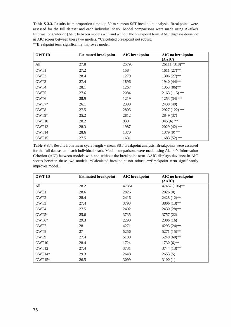
76
Table S 3.3. Results from proportion time top 50 m ~ mean SST breakpoint analysis. Breakpoints were
assessed for the full dataset and each individual shark. Model comparisons were made using Akaike's
Information Criterion (AIC) between models with and without the breakpoint term. ΔAIC displays deviance
in AIC scores between these two models. *Calculated breakpoint not robust.
**Breakpoint term significantly improves model.
OWT ID Estimated breakpoint AIC breakpoint AIC no breakpoint
(ΔAIC)
All 27.8 25793 26111 (318)**
OWT1 27.2 1584 1611 (27)**
OWT2 28.4 1279 1306 (27)**
OWT3 27.4 1896 1940 (44)**
OWT4 28.1 1267 1353 (86)**
OWT5 27.6 2084 2163 (115) **
OWT6 28.9 1219 1253 (34) **
OWT7* 26.1 2390 2430 (40)
OWT8 27.5 2805 2927 (122) **
OWT9* 25.2 2812 2849 (37)
OWT10 28.2 939 945 (6) **
OWT12 28.3 1987 2029 (42) **
OWT14 28.6 1370 1379 (9) **
OWT15 27.5 1631 1683 (52) **
Table S 3.4. Results from mean cycle length ~ mean SST breakpoint analysis. Breakpoints were assessed
for the full dataset and each individual shark. Model comparisons were made using Akaike's Information
Criterion (AIC) between models with and without the breakpoint term. ΔAIC displays deviance in AIC
scores between these two models. *Calculated breakpoint not robust. **Breakpoint term significantly
improves model.
OWT ID Estimated breakpoint AIC breakpoint AIC no breakpoint
(ΔAIC)
All 28.2 47351 47457 (106)**
OWT1 28.6 2826 2826 (0)
OWT2 28.4 2416 2428 (12)**
OWT3 27.4 3793 3806 (13)**
OWT4 27.5 2402 2430 (28)**
OWT5* 25.6 3735 3757 (22)
OWT6* 29.3 2290 2306 (16)
OWT7 28 4271 4295 (24)**
OWT8 27 5256 5271 (15)**
OWT9 27.4 5180 5240 (60)**
OWT10 28.4 1724 1730 (6)**
OWT12 27.4 3731 3744 (13)**
OWT14* 29.3 2648 2653 (5)
OWT15* 26.5 3099 3100 (1)

77
(a)
(b)

78
(c)
(d)
Figure S 3-1. The relationship between daily averaged vertical movement behaviours and SST for each
individual OWT. (a) Mean daily depth; (b) percentage time in the top 50 m; (c) mean cycle length (seconds);
and (d) mean amplitude.

79
Chapter 4 Biologging tags reveal the fine-
scale movement behaviours of
tiger sharks
4.1 Abstract
An understanding of the role that large marine predators play in structuring trophic flow and
nutrient cycling in marine ecosystems requires knowledge of their fine-scale (m-km) movement
behaviours. In this study, we explore the extent to which biologging tags reveal new insights into
the fine-scale movement ecology of tiger sharks (Galeocerdo cuvier) at Ningaloo Reef, Western
Australia. Tags deployed on 21 sharks for durations of 5-48 hours recorded both physical
parameters such as depth and temperature, and, through the use of accelerometers, gyroscopes
and compasses, in-situ measurements of animal trajectory and locomotion. Animal-borne-video
enabled the validation of behavioural signatures, mapping of habitat, and interactions with prey
to be recorded. Collectively, we used this data to examine the link between vertical (oscillations)
and horizontal (tortuosity) movements, and link sensor data to prey interactions recorded by the
video. Our biologging approach revealed complex movements that would otherwise be invisible
within the time-depth records provided by traditional tagging techniques. We found no
relationship between path tortuosity and vertical movements, suggesting that vertical movements
occur independently of search behaviours. Tiger sharks displayed tortuous movements possibly
associated with prey searching for 27% of their tracks, and interactions with prey elicited varied
responses including highly tortuous paths and burst movements. Accurate speed measurements
and GPS anchor points will considerably enhance the value of magnetometer data in future studies
by facilitating more accurate dead-reckoning and geo-referencing of area-restricted search
behaviours.
4.2 Introduction
The movement patterns of large marine predators such as tiger sharks (Galeocerdo cuvier) have
typically been sampled using acoustic telemetry and satellite tagging approaches (Andrews et al.
2009; Papastamatiou et al. 2009; Barnett et al. 2010; Brunnschweiler et al. 2010; Vaudo et al.
2014; Comfort and Weng 2015; Heupel and Simpfendorfer 2015; Papastamatiou et al. 2015a).
These studies generate either presence/absence data sets (acoustic telemetry), or movement
patterns of animals over large horizontal spatial scales (satellite tagging, 10s – 1000s km).
Although such studies continue to transform our understanding of the ecology and biology of
these animals (Chapman et al. 2015), they have two major shortcomings. Firstly, they provide
limited opportunities to identify and categorize behavioural modes at the fine spatial scales (m –

80
km) relevant to predator-prey and other inter and intraspecific interactions (competition, social
behaviours, cannibalism etc.) (Gleiss et al. 2009a). Secondly, the time-depth records that are
usually recorded by these techniques offer only coarse resolution of the patterns of vertical
movements of these predators through the water column (Ryan et al. 2004). Given that the
behaviour of large marine predators is thought to have a major role in structuring trophic flows
and nutrient cycling within marine ecosystems (Heithaus et al. 2008; Lavery et al. 2010), it is
imperative that we link their large-scale movement patterns with their day-to-day behaviours
within the environment.
Biologging approaches offer a means to achieve this aim. Tags such as the daily diary (Wilson et
al. 2008) incorporate a range of sensors including accelerometers and physical sensors, and can
be used to characterize fundamental aspects of the behaviour of individuals through quantitative
measurement of body kinematics. The combination of these sensors can therefore record detailed
movements of a target species as well as the environmental context in which they occur. First
used on marine animals in the late 1990s (Yoda et al. 1999), tri-axial accelerometers are often
incorporated into biologging devices, and have allowed researchers to categorise the behaviours
of sharks, including swimming, bursting, resting, and mating, and have also been used to quantify
activity patterns and the swimming energetics of vertical movements (Whitney et al. 2010; Gleiss
et al. 2011b; Whitney et al. 2012; Meekan et al. 2015). However, to link these fine-scale
behaviours to larger-scale movements, we need to understand how they relate to an animal’s path
through the environment. Accelerometers do not provide information on animal heading, limiting
most analysis of behaviours to a two-dimensional plane. Furthermore, the direct observation and
consequent validation of behaviours recorded by these sensors is almost impossible for a number
of large species of shark due to their high mobility and cryptic nature. The recent addition of
magnetometers and animal-borne cameras to biologging tags overcomes these issues. When used
in tandem with accelerometers, tri-axial magnetometers enable the reconstruction of movements
in three dimensions through the process of dead-reckoning (Wilson et al. 2008; Walker et al.
2015; Williams et al. 2017a). Animal-borne cameras add the ability to validate classifications of
behavioural signatures recorded by tri-axial sensors (Davis et al. 1999; Heithaus et al. 2001;
Narazaki et al. 2013) and enable interactions with prey to be recorded (Heithaus et al. 2002b;
Nakamura et al. 2015a; Papastamatiou et al. 2019).
Here, we use a biologging approach to examine the fine-scale movement and behaviour of the
tiger shark at Ningaloo Reef, Western Australia. Tiger sharks are a partial migrator, where some
individuals remain resident in coastal areas for long periods of time and others undertake long
distance movements (Meyer et al. 2010; Ferreira et al. 2015; Acuña-Marrero et al. 2017). Recent
studies have revealed that this species continuously oscillates through the water column, driven
by the need to either conserve energy, or search for benthic prey on descent, and silhouetted air-
breathing prey on ascent (Heithaus et al. 2002b; Nakamura et al. 2011).
81
In this study, we explore the extent to which multiple sensors in biologging tags reveal new
insights into the fine-scale movement ecology of tiger sharks. Our tags combined video,
environmental sensors, tri-axial accelerometers, magnetometers, and gyroscopes, allowing us to
classify behavioural signatures in vertical movements, validated by the video, and reconstruct
three-dimensional reconstructed paths of these animals while concurrently recording the
environmental context in which they occurred. This allowed us to (1) examine the relationship
between vertical (oscillations) and horizontal (tortuosity) movements, and (2) link sensor data,
including tailbeats, burst acceleration and tortuosity, to prey interactions recorded on video,
collectively identifying likely prey-searching behaviours.
4.3 Methods
4.3.1 Ethics
All methods were used in accordance with approved guidelines by the University of Western
Australia Animal Ethics Committee (RA/3/100/1437), and under permit numbers 2881 (WA
Department of Fisheries) and 08-000322-3 (WA Department of Parks and Wildlife).
Table 4-1. Terms and definitions used repetitively throughout chapter
Term Definition
Diving Ratio The proportion of time spent moving vertically (ascending or descending) within a
15 minute window
𝑅 Mean resultant length. A measure of the concentration of the heading data. When 𝑅
is equal to or close to one, points are closely clustered around the mean direction.
When 𝑅 approaches zero, points are spread more evenly in a circle.
Pseudo-track An approximation of a tiger shark’s horizontal track.
Inshore Inside the reef lagoon in depths of <25 m.
Offshore Outside the reef lagoon in depths of >25 m.
VV Vertical velocity (m/s)

82
4.3.2 Data collection
Tiger sharks were captured using baited drumlines inside the reef lagoon at Ningaloo Reef,
Western Australia (22.99°S, 113.8°E, Figure 1a) in April-May 2017. Drumlines were equipped
with a single 20/0 circle hook baited with fish scraps. Three drumlines were deployed
approximately 100 m apart between 07:00 and 16:00, with lines checked every hour for captures.
Once a shark was caught, it was secured alongside a 5.8 m vessel with the leader and a tail rope.
Each shark was measured (pre-caudal length, fork length, total length and maximum girth) and
its sex recorded, before a biologging tag was clamped to the base of its dorsal fin (Figure 4.1).
The dorsal fin of each shark was also photographed before and after tagging for identification
purposes and to assess any potential tag effects.
Figure 4.1. Tagged tiger sharks at Ningaloo Reef. (a) Tiger shark post-release. Photo courtesy of Alex
Kydd. (b) CATS Cam tag clamped to the dorsal fin. (c) CATS Diary tag clamped to the dorsal fin. (d)
Location of tag deployments.
83
A combination of CATS Diary tags (Customised Animal Tracking Solutions, Australia) and
CATS Cam tags were deployed on tiger sharks (Figure 4.1). Both were equipped with tri-axial
accelerometers, magnetometers, and gyroscopes, and depth, temperature and light sensors. In
addition, the Cam tag housed a HD video camera. The sensors continuously recorded all
parameters at 20 Hz, and video was recorded at pre-programmed hours of the day for a maximum
of six hours per deployment, due to storage limitations. In order to attach the tags to the dorsal
fins of the sharks, CATS tags were joined to a stainless steel spring clamp (CATS, Australia) via
a docking pin and a corrodible galvanic timed release (GTR, Ocean Appliances, Australia).
Previous work has shown that these clamps allow tags to remain rigidly attached to dorsal fins of
large sharks for up to 93 hours (Gleiss et al. 2009b; Chapple et al. 2015), and the GTR models
used were designed to dissolve in seawater after 7-48 hours (Table 4-2). Once the GTR dissolved,
the tag released from the clamp, allowing the tag to float to the surface. Floating tag packages
were tracked down using a hand-held VHF receiver operated from a vessel (Lear and Whitney
2016). A magnesium sleeve on the clamp itself also dissolved after approximately seven days, so
that the clamp detached, leaving no tagging equipment attached to the shark.
4.3.3 Data processing and analysis
Data recorded by the tags were processed to obtain a number of parameters classifying shark
movements and behaviours. The depth record was firstly split into vertical phases of ascent,
descent and constant depth. Tri-axial sensor data were then used to calculate the pitch angles of
vertical movements, overall dynamic body acceleration (ODBA), the acceleration signal
amplitude and frequency of tailbeats, and gliding behaviour. Tailbeat data were used to calculate
the recovery from capture following methods outlined by Whitney et al. (2016b). Tri-axial data
were also used to calculate shark heading, turning angles and other measures of track tortuosity.
Lastly, video data were used to record interactions with prey, determine habitat types, and validate
behaviours recorded by the sensors (e.g. tailbeats and bursting behaviour). The following
describes these methods in greater detail.
4.3.3.1 Depth record
Zero offset corrections were applied to the depth trace based on periods where sharks were being
tagged and known to be at the surface. The depth record was then split into vertical swimming
phases (‘ascending’, ’descending’ and ‘level swimming’) using vertical velocity (VV). To do this,
the depth trace was firstly smoothed using a ten second running mean and the average VV was
calculated by taking the difference of this smoothed depth between successive points at one
second intervals. Ascents and descents were defined where VV exceeded an absolute value of
0.05 m/s for more than ten seconds, and level where this value was not exceeded (Whitney et al.
2016b).
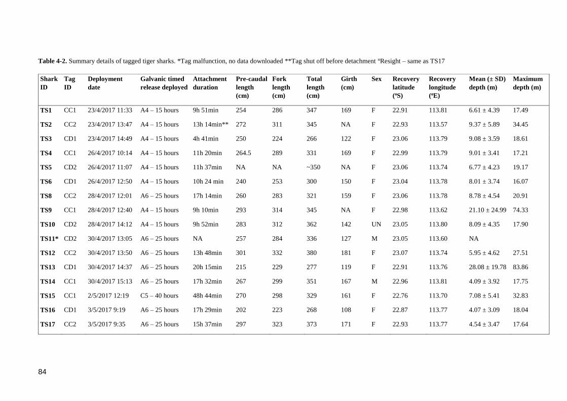
84
Table 4-2. Summary details of tagged tiger sharks. *Tag malfunction, no data downloaded **Tag shut off before detachment nResight – same as TS17
Shark
ID
Tag
ID
Deployment
date
Galvanic timed
release deployed
Attachment
duration
Pre-caudal
length
(cm)
Fork
length
(cm)
Total
length
(cm)
Girth
(cm)
Sex Recovery
latitude
(oS)
Recovery
longitude
(oE)
Mean (± SD)
depth (m)
Maximum
depth (m)
TS1 CC1 23/4/2017 11:33 A4 – 15 hours 9h 51min 254 286 347 169 F 22.91 113.81 6.61 ± 4.39 17.49
TS2 CC2 23/4/2017 13:47 A4 – 15 hours 13h 14min** 272 311 345 NA F 22.93 113.57 9.37 ± 5.89 34.45
TS3 CD1 23/4/2017 14:49 A4 – 15 hours 4h 41min 250 224 266 122 F 23.06 113.79 9.08 ± 3.59 18.61
TS4 CC1 26/4/2017 10:14 A4 – 15 hours 11h 20min 264.5 289 331 169 F 22.99 113.79 9.01 ± 3.41 17.21
TS5 CD2 26/4/2017 11:07 A4 – 15 hours 11h 37min NA NA ~350 NA F 23.06 113.74 6.77 ± 4.23 19.17
TS6 CD1 26/4/2017 12:50 A4 – 15 hours 10h 24 min 240 253 300 150 F 23.04 113.78 8.01 ± 3.74 16.07
TS8 CC2 28/4/2017 12:01 A6 – 25 hours 17h 14min 260 283 321 159 F 23.06 113.78 8.78 ± 4.54 20.91
TS9 CC1 28/4/2017 12:40 A4 – 15 hours 9h 10min 293 314 345 NA F 22.98 113.62 21.10 ± 24.99 74.33
TS10 CD2 28/4/2017 14:12 A4 – 15 hours 9h 52min 283 312 362 142 UN 23.05 113.80 8.09 ± 4.35 17.90
TS11* CD2 30/4/2017 13:05 A6 – 25 hours NA 257 284 336 127 M 23.05 113.60 NA
TS12 CC2 30/4/2017 13:50 A6 – 25 hours 13h 48min 301 332 380 181 F 23.07 113.74 5.95 ± 4.62 27.51
TS13 CD1 30/4/2017 14:37 A6 – 25 hours 20h 15min 215 229 277 119 F 22.91 113.76 28.08 ± 19.78 83.86
TS14 CC1 30/4/2017 15:13 A6 – 25 hours 17h 32min 267 299 351 167 M 22.96 113.81 4.09 ± 3.92 17.75
TS15 CC1 2/5/2017 12:19 C5 – 40 hours 48h 44min 270 298 329 161 F 22.76 113.70 7.08 ± 5.41 32.83
TS16 CD1 3/5/2017 9:19 A6 – 25 hours 17h 29min 202 223 268 108 F 22.87 113.77 4.07 ± 3.09 18.04
TS17 CC2 3/5/2017 9:35 A6 – 25 hours 15h 37min 297 323 373 171 F 22.93 113.77 4.54 ± 3.47 17.64
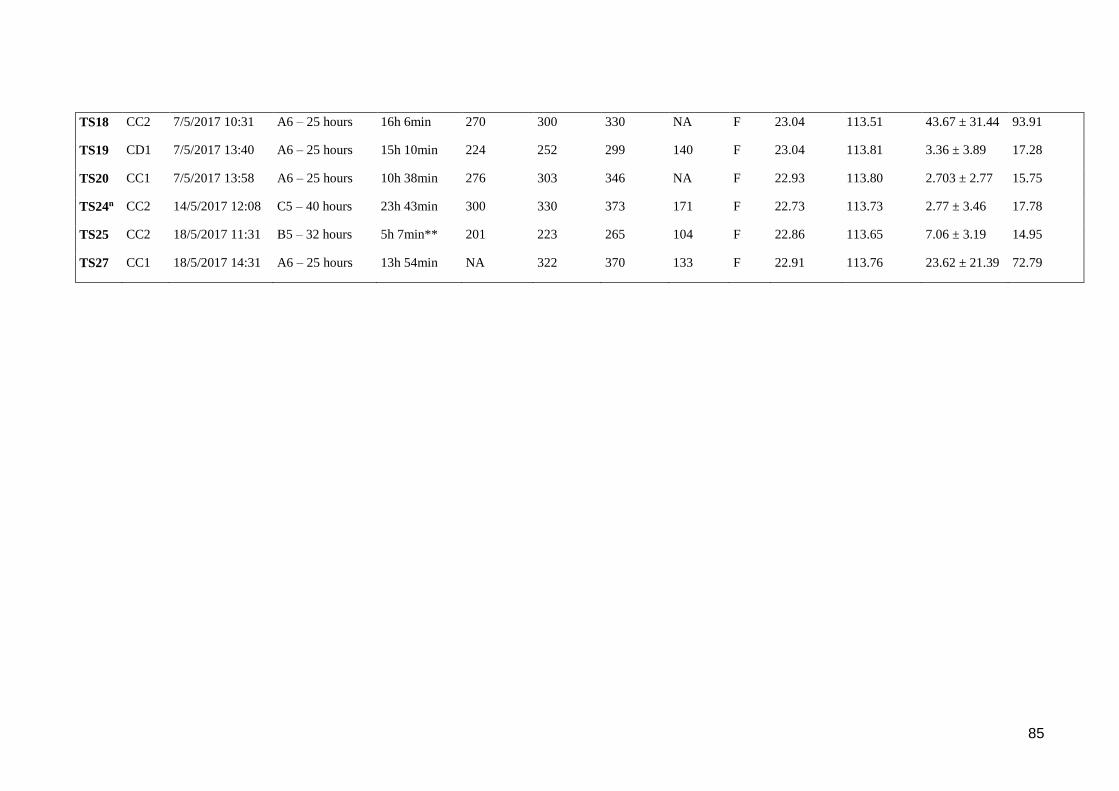
85
TS18 CC2 7/5/2017 10:31 A6 – 25 hours 16h 6min 270 300 330 NA F 23.04 113.51 43.67 ± 31.44 93.91
TS19 CD1 7/5/2017 13:40 A6 – 25 hours 15h 10min 224 252 299 140 F 23.04 113.81 3.36 ± 3.89 17.28
TS20 CC1 7/5/2017 13:58 A6 – 25 hours 10h 38min 276 303 346 NA F 22.93 113.80 2.703 ± 2.77 15.75
TS24n CC2 14/5/2017 12:08 C5 – 40 hours 23h 43min 300 330 373 171 F 22.73 113.73 2.77 ± 3.46 17.78
TS25 CC2 18/5/2017 11:31 B5 – 32 hours 5h 7min** 201 223 265 104 F 22.86 113.65 7.06 ± 3.19 14.95
TS27 CC1 18/5/2017 14:31 A6 – 25 hours 13h 54min NA 322 370 133 F 22.91 113.76 23.62 ± 21.39 72.79

86
4.3.3.2 Tri-axial sensor data
Data recorded by the accelerometer (acceleration) and gyroscope (angular velocity) were analysed
using Igor Pro ver. 7.0.4.1 (Wavemetrics, Inc. Lake Oswego, USA) and Ethographer (Sakamoto
et al. 2009). The gravitational component of acceleration (static acceleration) was determined
using a three second box smoothing window on the raw acceleration data (Shepard et al. 2008).
Pitch angles were derived by calculating the arcsine of the static acceleration in the surging
(posterior-anterior) axis. To correct for the tag attachment angle on each individual shark, we
determined the pitch when the shark was swimming at a constant depth (when VV was equal to
zero), and subtracted this value from all pitch estimates (Kawatsu et al. 2009). ODBA (overall
dynamic body acceleration) was calculated by summing the absolute value of dynamic
acceleration from all three axes (Wilson et al. 2006). Comparing ODBA with video recorded burst
events allowed us to classify bursts as events where ODBA >0.2. The dynamic component of
acceleration was calculated by subtracting the gravitational component from the raw acceleration
for each axis. We used a continuous wavelet transformation on the dynamic component of sway
(lateral) axis to calculate the acceleration signal amplitude and frequency of tailbeats (Sakamoto
et al. 2009). Using these same methods, angular velocity signal amplitude and frequency were
calculated using the angular velocity data, and the resulting signals were compared with those
derived from the acceleration data to determine the best measure of tailbeats.
4.3.3.3 Recovery period
We used metrics quantifying tailbeat activity calculated from tri-axial sensor data to estimate the
duration of recovery from stress of capture following the methods of Whitney et al. (2016b). This
study found that immediately after release, the tailbeats of blacktip sharks Carcharhinus limbatus
were elevated, and would slowly decline in frequency over the course of an individual’s recovery.
Briefly, to calculate this period for tiger sharks, tailbeat cycle (the inverse of tailbeat frequency)
throughout descent was summarized for 15 minute windows, and plotted against time post-
release. A recovery period was defined as the time it took for this metric to reach 80% of its
asymptote (Whitney et al. 2016b). This recovery period was eliminated from the data prior to
further analyses to remove potential sublethal and unnatural behaviours resulting from stress of
capture by drumlines.
4.3.3.4 Shark heading and pseudo-track calculation
Acceleration and magnetometer data were used to calculate head yaw angle (hereafter referred to
as ‘heading’) and pseudo-tracks in the software Framework 4 (Walker et al. 2015). Heading
calculations required input of orientation of the sensors in the tags, and magnetometer and
acceleration data. The orientation of the device was corrected using orientation specifications
provided by CATS (N. Liebsch pers. comm). The coordinate systems of the accelerometer and
87
magnetometer were perfectly aligned and consequently no adjustment was required to align these
sensors. Pitch and roll calculated from the accelerometer data were used to correct for tilt (Walker
et al. 2015). In addition to the calculations applied by Framework 4, we applied a three second
box smoothing window to the heading data to filter out the dynamic movements of the sharks
caused by tailbeats.
Heading was used to calculate pseudo-tracks for each shark. These tracks were used only for
plotting short-term movements of the sharks in three-dimensional space. They could not be used
to estimate accurate locations of the tagged sharks due to the accumulation of errors from the
estimates of heading and speed over the course of the dead-reckoned track (Wilson et al. 2007;
Walker et al. 2015). Heading data were also used to calculate the turning angles of individuals on
a between-second basis. Data were resampled to a one second frequency and converted to a 0-
360o scale. The minimum difference in angle between consecutive observations was used to
determine turning angle.
4.3.3.5 Window size and statistics
The time window used for analysis was selected by determining the window for which the highest
variance in turning angle was observed, while being of sufficient width to capture the longest
dives in their entirety. This time window was estimated to be 15 minutes, and within this period,
a number of vertical movement parameters were summarized including mean (± standard
deviation) and maximum depth, ascent pitch, descent pitch, ascent VV and descent VV. The
percent of time spent moving vertically (ascending and descending), termed the ‘diving ratio’,
was also calculated for each window. In addition, heading was used to calculate measurements of
path tortuosity and direction. Firstly, turning angles were summed for each window to obtain an
estimate of tortuosity. Secondly, the Circular package in R was used to calculate the mean
resultant length, or 𝑅, of the heading, a measure of the concentration of unimodal circular data
(Pewsey et al. 2013). When 𝑅 is close to or equal to one, points are closely clustered around the
mean direction and are highly directional, and as 𝑅 approaches zero, points spread more evenly
in a circle indicative of a tortuous path.
4.3.3.6 Video analysis
Video recorded by the tags was analysed in BORIS (Behavioural Observation Research
Interactive Software; Friard and Gamba 2016). This open-source software allows the user to set
an ethogram and record the timing of behavioural events. We set an ethogram to mark the
occurrence of prey interactions, shark responses to the presence of prey, burst swimming events,
presence of seabed in the field of view, habitat type, and other notable behaviours (Table S 4.1).
Video was also used to validate parameters recorded and calculated from the diary data, such as
tailbeat frequency, bursts and glides.

88
4.3.3.7 Movement classification
Hierarchical cluster analysis was used to categorize both vertical movements and path tortuosity
for each analysis window in the software R 3.4.0 (R Core Team 2017). Vertical movements were
classified using mean ascent and descent pitch, and diving ratio, and the path tortuosity using the
sum of the turning angles and 𝑅. These variables were scaled using the scale function in R and a
cluster analysis was applied using the hclust function, based on a dissimilarity matrix produced
from Euclidean distances and complete linkage as the agglomeration method. We chose the
number of clusters by looking at the gradient of reduction in within groups sum of squares with
additional number of clusters added. Groups resulting from the clustering of vertical movements
were labelled as ‘V-groups’ and from the clustering of path tortuosity as ‘T-groups’. The resulting
V-groups were compared through qualitative analysis and correlation coefficients with T-groups
to investigate if more tortuous movements were related to more oscillatory movements. Where
movements were identified to be tortuous, available behavioural records from concurrent videos
were examined.
4.3.3.8 Generalised linear mixed models (GLMMs)
To further investigate relationships between oscillatory and tortuous movements, generalised
linear mixed models (GLMMs) were built in R using the nlme package (Pinheiro et al. 2017).
Diving ratio was set as the response variable, 𝑅 and sum of turning angles were sequentially set
as explanatory variables (due to correlation >0.6 between these variables), and tiger shark identity
was set as a random variable. Diving ratio was logit transformed prior to analysis. We used the
corAR1 function to account for temporal auto-correlation in our datasets (Zuur et al. 2009). The
resulting models were compared with null models using Akaike’s information criterion (AIC).
4.4 Results
A total of 22 tiger sharks ranging in length from 2.65 – 3.8 m TL were caught and tagged (14
camera tag and 8 daily diary tag deployments) (Table 4-2). Tags were attached for a mean duration
of 15 hours (range 4.5-48 hours) and recorded approximately 410 hours of diary data and 50 hours
of video footage. One diary tag failed to record any data. One shark was recaptured after 11 days
and was re-tagged (TS17 and TS24 in Table 4-2). Based on an analysis of tailbeats, we assumed
a recovery period from capture and tagging by the sharks of four hours and for this reason, the
first four hours of each dataset were excluded from further analysis (Figure S 4-1). Evidence for
recovery after this time was also provided by the video records, which showed investigations of
potential prey and consumption of a discarded fish head by sharks within two hours of tagging
and release (Supplementary Video 1). The angular velocity data produced the clearest tailbeat
signal and was therefore used for further data exploration.

89
4.4.1 Vertical movements
The seabed was observed in videos at least every 15 minutes in all but 14 (~2%) sampling
windows where the water visibility was very poor, or in one case, during a period of extended
surface swimming by a shark while offshore. As a result, we assumed that vertical oscillations
were depth-limited and could be used to map the approximate depth of the seabed throughout the
tracks (Figure S 4-2). Tagged tiger sharks swam at a mean depth of 11.6 ± 17.5 m, predominately
remaining in inshore habitats, with four tiger sharks moving into offshore habitats and diving to
a maximum depth of 94 m. Video analysis showed tiger sharks transiting a variety of habitats,
including sand, macroalgal reefs, coral reef, bare reef, pelagic, and edge habitats (Bancroft 2003)
(Supplementary Video 1).
The cluster analysis revealed six vertical-groupings (V-groups) as the dominant vertical
movement modes, with an additional six V-groups describing <8% of the data (Figure 4.2,

90
Table S 4.2). Diving ratio increased from 0.5 ± 0.8% in V-group 1 to 80 ± 6% in Group 8. Groups
4, 5 and 7 were characterized by mean diving ratio and/or mean pitch that were greater than overall
mean values, and examination of tracks associated with these groups demonstrated that they were
associated with a higher frequency of oscillations throughout the water column. Offshore periods
were only clustered into these three V-groups, whereas all modes of vertical movement were
displayed by inshore sharks.
4.4.2 Horizontal path tortuosity
The classification of path tortuosity generated seven tortuosity-groups (T-groups) (Figure 4.2,
Table S 4.3). Movements increased in tortuosity from T-groups 1-7, ranging from highly
directional with low turning to almost uniform distributions of direction with high levels of
turning. A total of 72.6% of windows were classified in T-groups 1-3 where movements were
categorized as directional and the remaining 27.4% in T-groups 4-7 were categorized as tortuous.
All T-groups were present in both inshore and offshore habitats.
Video cameras were recording for 21 of the windows assessed to have tortuous paths. For almost
half of these windows (43%), tiger sharks were located on the shallow sandflats (<3 m in depth).
Six tortuous windows were associated with investigations of turtles. For example, TS15 was
tracking through coral reef habitat when a loggerhead turtle (Caretta caretta) was sighted on the
far right of the field of view (Figure 4.3, Supplementary Video 1). After this first observation, the
shark turned sharply and the turtle was again spotted in mid-water, tightly turning away from the
shark with its shell perpendicular to the shark. The shark then approached the surface and
descended before circling the same area of coral reef for 25 minutes, remaining on the seabed and
following the structure of the reef (Figure 4.3, Supplementary Video 1). The turtle was not
observed again in the field of view for the remainder of this 25 minute period.

91
Figure 4.2. Comparison of dominant vertical movement clusters (V-groups) and path tortuosity clusters
(T-groups) from hierarchical cluster analysis. (a) 15 minute depth profiles representative of V-groups 1, 3
and 6, demonstrating the increase in oscillatory movements with V-group. (b) 15 minute pseudo-tracks
representative of each T-group, demonstrating the increase in tortuosity with T-group. Polar plot on bottom
right of each track displays example of heading variance for each group. (c) The % windows found in each
cluster. (d) The % T-group composition of each dominant V-group. Colours are T-groups from (b).

92
Figure 4.3. Tiger shark and loggerhead turtle interaction. (a) One-hour long pseudo-track from TS15. Red
square denotes area of prey interaction displayed in (b) and (c). (b) Depth track. (c) 3D track. (d)
Screenshots from video of the interaction. 1 and 2 refer to where interaction takes place in depth and 3D
tracks. See Supplementary Video 1 for full video of interaction.
A number of other interactions with prey were recorded on the cameras (Table S 4.4), however
none of these involved successful foraging on live prey. Most interactions (92%) occurred when
sharks were level swimming with the seabed in the field of view of the camera and included
investigations and possible stalking of several lutjanid fish (Symphorus nematophorus), in at least
one case prompting a rapid colour change, 17 interactions with turtles, in at least four cases
eliciting tight turning and shell up responses from turtles, and potential investigations of a tawny
nurse shark (Nebrius ferrugineus) and another tiger shark (Table S 4.4 & Supplementary Video
1). Several investigations of prey were immediately preceded by burst, stalking and/or turning
behaviours (Figure 4.4). Sharks did not pursue vigilant or fleeing prey, and no bursts were
observed in the direction of prey when prey were in the field of view.
No extended periods of bursting that may be indicative of headshaking behaviour (bursts greater
than two seconds in length; Brewster et al. 2018) were observed in any part of the dataset. Burst
behaviour was highly variable with a mean 3 ± 15 bursts occurring in a 15 minute window. Highly
tortuous windows (T-groups 6 and 7) were associated with higher than average bursts (e.g. Figure
4.6), however further analysis of bursting was confounded by artificially high ODBA levels when
swimming at the surface due to the effects of chop.

93
Table 4-3. Results of generalised linear mixed models testing the relationship between diving ratio and
indicators of horizontal path tortuosity. Diving ratio was logit transformed prior to analysis. All models
were compared with null models using Akaike’s Information Criterion (AIC) and conditional (R2c) and
marginal (R2m) R2 values. All models were run using the nlme package in R with shark identity as a random
variable. All null models include the random effect
Inshore Model DF AIC R2m R2c
Diving Ratio ~ 𝑅 865 2340 0.001 0.51
Diving Ratio ~ 1 866 2339 0 0.51
Diving Ratio ~ Sum of turning angles 865 2361 0.0002 0.51
Diving Ratio ~ 1 866 2339 0 0.51
Figure 4.4. One minute pseudo-tracks of tiger shark and Chinamanfish (Symphorus nematophorus)
interactions. Track line is coloured by tailbeat frequency (Hz). Red dashed square indicates where the fish
was observed in the video field of view (displayed in screenshots to the right of the pseudo-track). X and
Y-axes represent arbitrary units of latitude and longitude created by magnetometer and accelerometer data
whilst a constant speed is assumed. (a) Example of an interaction where the tailbeat of the shark slows upon
encountering the fish. (b) Example of an interaction where the tailbeat of the shark quickens upon
encountering the fish.

94
4.4.3 Oscillations and tortuosity
There were no strong correlations between vertical movement and tortuosity variables (all r <0.3)
and almost all vertical movements displayed all levels of tortuosity. For example, highly
oscillatory movements classified in V-group 8 were classified in both T-group 1 with directional
swimming, and in T-group 6 where movements were highly tortuous (Figure 4.5). Conversely,
Figure 4.6. 15 minute pseudo-track throughout a tortuous window in TS20. Track is coloured by bursts
(ODBA>0.2) and takes place at approximately 21:30 in water approximately 2 m in depth.
Figure 4.5. Two tiger sharks (i & ii) with very similar oscillatory depth tracks but different horizontal tracks
in offshore environments over a 2.5 hour period. (a) Depth track. (b) Pseudo-track. (c) 3D track.

95
windows containing entirely level swimming in V-group 1 were also classified in both T-groups
1 and 6. In addition, generalized linear mixed models revealed no relationships between diving
ratio and variables describing tortuosity (𝑅 and sum of turning angles, Table 4-3).
4.5 Discussion
Our study shows how a multi-sensor biologging approach may be used to investigate foraging
behaviour of sharks as large, top-order predators. This information is essential if we are to
understand the keystone role that these animals are thought to play in marine ecosystems.
4.5.1 Foraging behaviour and tortuosity
We found evidence of foraging behaviour based on path tortuosity and video recorded encounters
with potential prey. Tiger sharks displayed tortuous horizontal paths for approximately 27% of
their tracks. As straight-line directional movement has been calculated to be the most
energetically efficient form of travel (Wilson et al. 2013), the initiation of tortuous movements
should provide some form of benefit to offset the energetic costs of turning. Tortuous movements
have been linked with searching behaviour and increased foraging success in many marine
animals, and are thought to indicate area-restricted searching (Kareiva and Odell 1987; Austin et
al. 2006; Papastamatiou et al. 2012; Adachi et al. 2017). For this reason, we argue that the tortuous
tracks we recorded represented prey searching, despite the fact that we did not witness any
consumption of prey. It should also be noted that the direct observation of natural predation events
by marine predators tends to be very rare (Pitman et al. 2014; Papastamatiou et al. 2019),
particularly for ectothermic shark species that are likely to feed less frequently compared to
marine mammals and seabirds (Papastamatiou et al. 2019). Given that video recordings were
limited to a maximum of six daylight hours per tag due to data storage and lighting constraints, it
is perhaps not surprising that we did not record any predation events involving live prey.
In addition, previous observations of foraging behaviour suggest that tiger sharks have a
preference for weakened and/or injured prey and rarely predate on vigilant animals (Heithaus et
al. 2002b; Hammerschlag et al. 2016). In several cases prey investigations were followed by either
escape maneuvers performed by turtles, or colour displays from demersal fish, all of which
culminated with the shark continuing on its course without attempting to predate on the alert
individual. It is also possible that some of these foraging behaviours may not have been focused
on the potential prey species that were seen in the video, particularly in the case of benthic fishes.
Facultative scavenging is an important feature of the behaviour of tiger sharks (Clua et al. 2013;
Hammerschlag et al. 2016) and in some cases sharks may have been drawn to approach
mesopredatory benthic fishes simply by the potential opportunity to scavenge food, i.e.

96
kleptoparasitism. This might explain why burst acceleration occurred during only sporadically in
prey investigations (Figure 4.4).
Video data showed that tortuous movements were often associated with shallow sandflat habitats,
a location where tiger sharks at Ningaloo Reef have frequently been observed hunting prey by
ecotourism operators (pers. comm Frazer McGregor, Figure S 4-3). It is possible that tiger sharks
may be showing a pattern of area-restricted search after detecting potential prey, either to
investigate this prey source or due to the high probability of encountering other prey items nearby,
or when entering areas linked to high foraging success based on past learning experiences (Adachi
et al. 2017). Similar patterns in exploratory foraging have been found in the movements of lions
(Panthera leo), where GPS-collared individuals exhibited more tortuous and slower movements
when in the vicinity of waterholes, a pattern that suggested area-restricted searching in an area
with potentially higher prey density (Valeix et al. 2010). In our study, sandflats may be preferred
habitats for foraging by tiger sharks because prey here have less room to perform evasive
maneuvers and to escape (Heithaus et al. 2002a), increasing the efficiency of hunting.
4.5.2 Three-dimensional movements
Fine-scale movement behaviours were invisible in the time-depth record. A comparison of
vertical and horizontal tracks of tagged tiger sharks found no relationship between vertical
movements and path tortuosity, and some tracks with the same time-depth record displayed very
different horizontal paths. Level or oscillatory swimming occurred while the shark displayed
either directional or tortuous swimming, suggesting that vertical movements may not change
significantly when undergoing area-restricted search. The majority of investigations (92%) of
potential prey occurred when tiger sharks were level swimming, with several of these taking place
during tortuous paths. Oscillatory behaviour was often observed prior to prey investigation events.
This behaviour suggests that sharks may have been searching the water column for visual or
olfactory cues (Carey et al. 1990; Klimley et al. 2002), and once triggered, began tortuous paths
in order to locate prey and to remain in a potentially profitable area. For example, one shark
encountered a loggerhead turtle on a small coral reef and then circled the same area for 25 minutes,
although the prey was not re-encountered. The variance in behaviours observed in similar depth
profiles highlights the need for a combination of high resolution tri-axial movement and depth
sensors to gain a full picture of the behaviour of these animals, as time-depth records alone would
be insufficient to distinguish prey searching and fine-scale habitat use.
4.5.3 Challenges and future considerations
Although biologging approaches provide a wealth of new information, there are many challenges
in processing, analyzing, visualizing and interpreting the large amount of data recorded by these
tags (Whitney et al. 2019). Manipulation of the datasets can require access to large computers and
97
proficiency in multiple types of specialist software and challenges also arise in visualizing the
data to display biologically relevant patterns within very complex data sets. Here, many of the
different data streams were shown to be important in understanding the fine-scale movement
behaviour of tiger sharks. Pseudo-tracks and three-dimensional plots presented a relatively simple
means to visualize the data, and both heading and tailbeat kinematic data were demonstrated to
be useful in describing interactions with prey. Such an approach is likely to be of use for
investigating and comparing these behaviours among other shark species, where differences in
foraging ecology may drive differences in prey searching behaviours and therefore three-
dimensional movement patterns.
Despite our biologging approach revealing detailed insights into movements and behaviours of
tiger sharks, interpretation of data sets was hampered by several issues. Firstly, the field of view
of the camera often limited our interpretation of behaviours, and was not likely to record all
interactions of sharks with prey. A wider field of view, or optimally cameras capable of filming
across 360° may enable further behavioural insights. Secondly, storage and battery constraints
and the need to recover the tags in order to download archived data sets constrained tag
deployments to relatively short periods (a few days at most). Delaying video activation until after
predicted recovery periods for sharks could assist in extending tag recording time. However, there
is no current solution to the need to recover the tags, which makes it difficult to place the fine-
scale movement patterns we described into a longer term context. Lastly, accurate speed
measurements and GPS anchor points would considerably increase the value of the magnetometer
data in allowing us to calculate more accurate fine-scale locational and habitat preferences, and
the incidence of area-restricted search (Walker et al. 2015).
4.5.4 Conclusion
Our study demonstrates the utility of multi-sensor biologging tags in classifying the fine-scale
movements and behaviours of a keystone marine predator. Our results showed that recording
movement in two-dimensions alone, as is the case with traditional time-depth recorders, will not
be sufficient in distinguishing among fine-scale behavioural modes. Data obtained from the
combination of magnetometers, accelerometers and video effectively described predator-prey
interactions and habitat use, providing important information about how these sharks interact with
their ecosystem. Such information will enable a greater understanding of the role these predators
play in coral reef ecosystems.
4.6 Acknowledgements
Fieldwork and tags were funded by crowdfunding on the Experiment platform (DOI:
10.18258/7190), a Holsworth Wildlife Research Endowment, a UWA Graduate Research School

98
fieldwork award and BigWave Productions. We thank Murdoch University and Coral Bay
Research Station for accommodation and vessel use while conducting fieldwork. This work
would not have been possible without the generous support of numerous volunteers, particularly:
Frazer McGregor, Abraham Sianipar, Adam Jolly, Blair Bentley, Evan Byrnes, Garry Teesdale
and Michael Tropiano providing valuable field support; Olivia Seeger and Abraham Sianipar who
helped with the video analysis. Nikolai Liebsch provided invaluable assistance with tag
functioning. Alex Kydd, David Palfrey and Daniel Thomas-Browne generously contributed
photos and video. Ryan Daly supplied helpful assistance for the analysis.

99
4.7 Supporting Information
Supplementary Video 1: https://vimeo.com/303181061
Password: shark
Figure S 4-1. Recovery period in tiger sharks after being caught and released. Black dots and error bars
represent mean tailbeat cycles (the inverse of tailbeat frequency) during descent for individual tiger sharks
over 15 minute windows. The solid blue line is the combined regression for all individuals, and the red
dashed line indicates the point at which the approximate 80% threshold was calculated, and individuals
were considered to be recovered. Methods follow that of Whitney et al. (2016b)
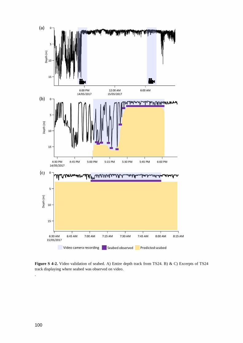
100
Figure S 4-2. Video validation of seabed. A) Entire depth track from TS24. B) & C) Excerpts of TS24
track displaying where seabed was observed on video.
.

101
Figure S 4-3. Interaction between a tiger shark and turtle in the sandflats around Coral Bay. Photos courtesy
of Daniel Thomas-Browne.
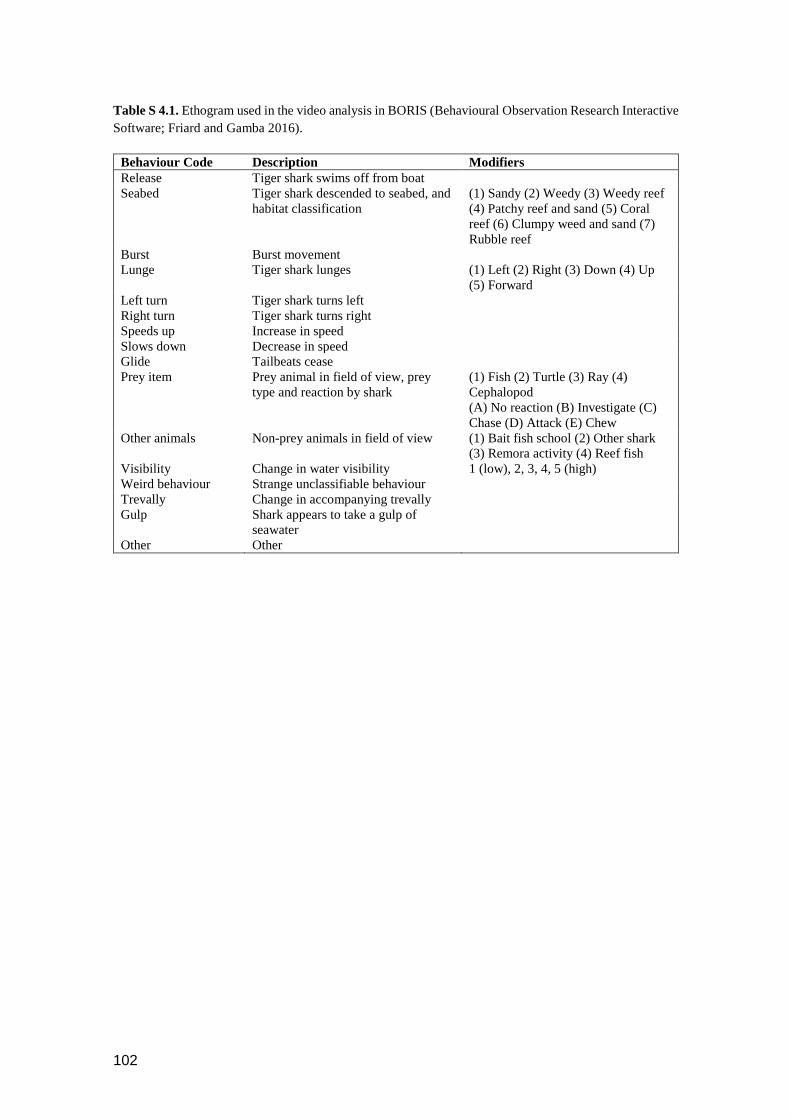
102
Table S 4.1. Ethogram used in the video analysis in BORIS (Behavioural Observation Research Interactive
Software; Friard and Gamba 2016).
Behaviour Code Description Modifiers
Release Tiger shark swims off from boat
Seabed Tiger shark descended to seabed, and
habitat classification
(1) Sandy (2) Weedy (3) Weedy reef
(4) Patchy reef and sand (5) Coral
reef (6) Clumpy weed and sand (7)
Rubble reef
Burst Burst movement
Lunge Tiger shark lunges (1) Left (2) Right (3) Down (4) Up
(5) Forward
Left turn Tiger shark turns left
Right turn Tiger shark turns right
Speeds up Increase in speed
Slows down Decrease in speed
Glide Tailbeats cease
Prey item Prey animal in field of view, prey
type and reaction by shark
(1) Fish (2) Turtle (3) Ray (4)
Cephalopod
(A) No reaction (B) Investigate (C)
Chase (D) Attack (E) Chew
Other animals Non-prey animals in field of view (1) Bait fish school (2) Other shark
(3) Remora activity (4) Reef fish
Visibility Change in water visibility 1 (low), 2, 3, 4, 5 (high)
Weird behaviour Strange unclassifiable behaviour
Trevally Change in accompanying trevally
Gulp Shark appears to take a gulp of
seawater
Other Other

103
Table S 4.2. Summarised characteristics of each V-group derived from the hierarchical cluster analysis.
Values are mean ± standard deviation.
Cluster
ID
No. % Vertical
ratio
Descent
Pitch
Ascent
Pitch
Description Example
G1 66 7.1 0.005 ±
0.008
-6.63 ±
2.02
4.07 ± 0.64 Very low vertical, low-med descent
angle, low ascent angle
TS24
G2 190 20.4 0.12 ± 0.09 -7.38 ±
1.83
7.24 ± 1.53 Low vertical, low-med descent
angle, med ascent angle
TS16, TS24
G3 15 1.6 0.32 ± 0.13 -19.73 ±
2.85
12.0 ± 2.20 Low-med vertical, high descent
angle, med ascent angle
TS15
G4 52 5.6 0.37 ± 0.14 -13.25 ±
1.63
13.22 ±
2.38
Low-med vertical, med-high
descent angle, med-high ascent
angle
TS15
G5 287 30.8 0.52 ± 0.13 -10.71 ±
1.83
8.88 ± 1.45 Med-high vertical, med descent
angle, low-med ascent angle
Most, TS2,
TS12
G6 40 4.3 0.65 ± 0.15 -17.91 ±
2.74
8.59 ± 1.78 Med-high vertical, med-high
descent angle, low-med ascent
angle
TS13
G7 143 15.3 0.24 ± 0.10 -10.90 ±
1.56
10.04 ±
1.69
Low-med vertical, med descent
angle, med ascent angle
TS15
G8 120 12.9 0.80 ± 0.06 -12.55 ±
2.37
11.18 ± 2.1 High vertical, med-high descent
angle, med-high ascent angle
TS27, TS13
G9 9 0.9 0.26 ± 0.12 -13.57 ±
1.40
4.87 ± 1.04 Low-med vertical, med descent
angle, low ascent angle
TS15
G10 7 0.8 0.35 ± 0.08 -27.32 ±
4.13
19.25 ±
1.77
Med vertical, high-very high
descent angle, high ascent angle
TS9
G11 1 0.1 0.82 -19.57 22.23 High vertical, high descent angle,
very high ascent angle
TS13
G12 3 0.3 0.18 ± 0.24 -5.80 15.31 ±
1.24
Low-med vertical, low descent
angle, med-high ascent angle
TS15, TS27

104
Table S 4.3. Summarised characteristics of each T-group derived from the hierarchical cluster analysis.
Values are mean ± standard deviation.
Cluster
ID
No. % 𝑹 Turning Description Example
1 351 37.6 0.93 ±
0.04
1489 ±
501 High 𝑅, low turning TS14, TS15, TS18
2 108 11.6 0.80 ±
0.08
4273 ±
820 Med-high 𝑅, med
turning
TS13, TS14, TS15
3 218 23.4 0.70 ±
0.1
2611 ±
987 Med-high 𝑅, low-med
turning
TS15, TS24, TS8
4 73 7.8 0.64 ±
0.10
7623 ±
1544 Med-high 𝑅, med-
high turning
TS13, TS19
5 93 10 0.33 ±
0.13
3603 ±
1193 Low-med 𝑅, low-med
turning
TS15, TS24
6 78 8.4 0.34 ±
0.13
6086 ±
1269 Low-med 𝑅, med-
high turning
TS13, TS15, TS5
7 12 1.3 0.35 ±
0.16
13031 ±
1431 Low-med 𝑅, high
turning
TS20
Table S 4.4. All predator-prey interactions recorded on CATS video tags
Shark
ID
Prey Shark
behaviour
Depth &
vertical phase
Habitat Observational notes
TS1 Turtle Investigate 14 m – level Sandy seabed Bad vis, veers towards it then
away
TS1 Trevally – F.
Carangidae
Investigate 13 m – level Sandy seabed Turn right towards it quickly
TS1 Chinamanfish -
Symphorus
nematophorus
Investigate 4 m – level Sandy seabed Slows down, stalks then veers
away
TS1 Tuskfish –
Choerodon sp.
Investigate 4.8 m – level Sandy and
weedy seabed
Slows down, investigates and
moves on
TS1 Spangled emperor
- Lethrinus
nebulosus
Investigate 4 m – level Sandy seabed Increases speed and turns left
towards fish, swims past
TS1 Chinamanfish -
Symphorus
nematophorus
Investigate 4 m – level Sandy with
weed clumps
Turn left, burst, slows down,
inspects fish and swims by
TS1 Chinamanfish -
Symphorus
nematophorus
Investigate 4 m – level Sandy seabed Turn left, speed up and inspect
from distance
TS1 Batfish - Platax
teira
Investigate 3 m – level Sandy seabed Burst, slowdown, slight turn
right as investigates
Tortuosity
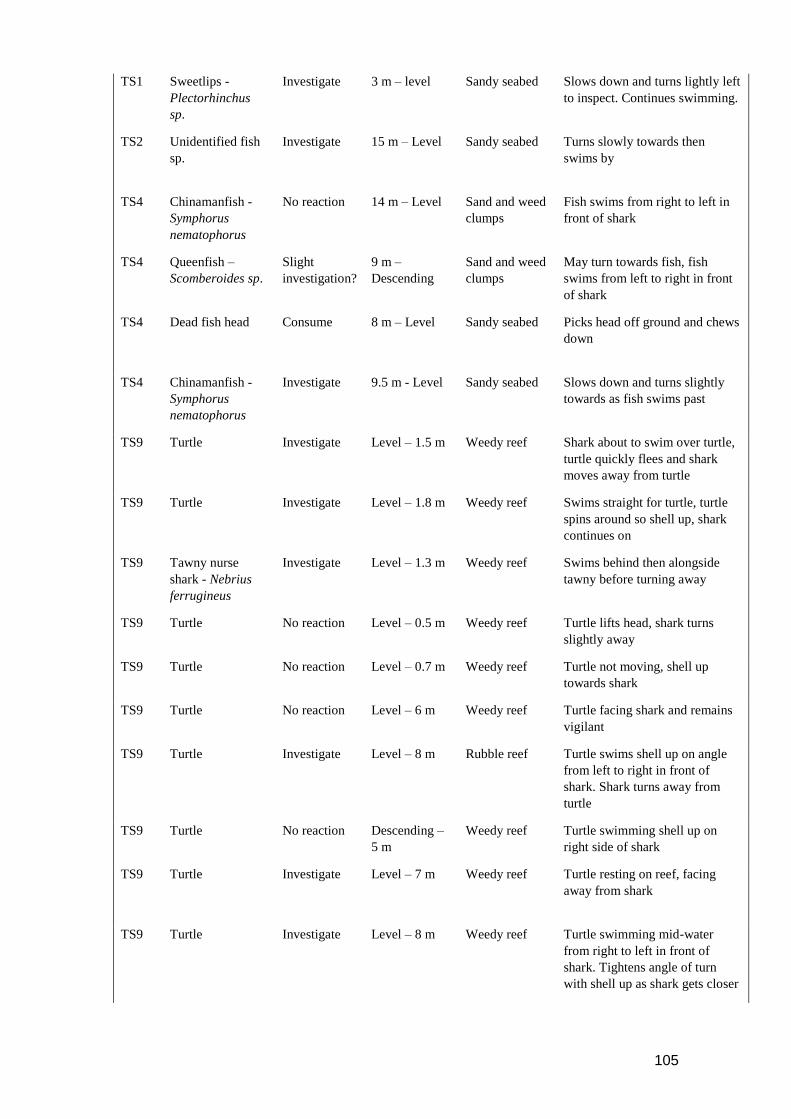
105
TS1 Sweetlips -
Plectorhinchus
sp.
Investigate 3 m – level Sandy seabed Slows down and turns lightly left
to inspect. Continues swimming.
TS2 Unidentified fish
sp.
Investigate 15 m – Level Sandy seabed Turns slowly towards then
swims by
TS4 Chinamanfish -
Symphorus
nematophorus
No reaction 14 m – Level Sand and weed
clumps
Fish swims from right to left in
front of shark
TS4 Queenfish –
Scomberoides sp.
Slight
investigation?
9 m –
Descending
Sand and weed
clumps
May turn towards fish, fish
swims from left to right in front
of shark
TS4 Dead fish head Consume 8 m – Level Sandy seabed Picks head off ground and chews
down
TS4 Chinamanfish -
Symphorus
nematophorus
Investigate 9.5 m - Level Sandy seabed Slows down and turns slightly
towards as fish swims past
TS9 Turtle Investigate Level – 1.5 m Weedy reef Shark about to swim over turtle,
turtle quickly flees and shark
moves away from turtle
TS9 Turtle Investigate Level – 1.8 m Weedy reef Swims straight for turtle, turtle
spins around so shell up, shark
continues on
TS9 Tawny nurse
shark - Nebrius
ferrugineus
Investigate Level – 1.3 m Weedy reef Swims behind then alongside
tawny before turning away
TS9 Turtle No reaction Level – 0.5 m Weedy reef Turtle lifts head, shark turns
slightly away
TS9 Turtle No reaction Level – 0.7 m Weedy reef Turtle not moving, shell up
towards shark
TS9 Turtle No reaction Level – 6 m Weedy reef Turtle facing shark and remains
vigilant
TS9 Turtle Investigate Level – 8 m Rubble reef Turtle swims shell up on angle
from left to right in front of
shark. Shark turns away from
turtle
TS9 Turtle No reaction Descending –
5 m
Weedy reef Turtle swimming shell up on
right side of shark
TS9 Turtle Investigate Level – 7 m Weedy reef Turtle resting on reef, facing
away from shark
TS9 Turtle Investigate Level – 8 m Weedy reef Turtle swimming mid-water
from right to left in front of
shark. Tightens angle of turn
with shell up as shark gets closer
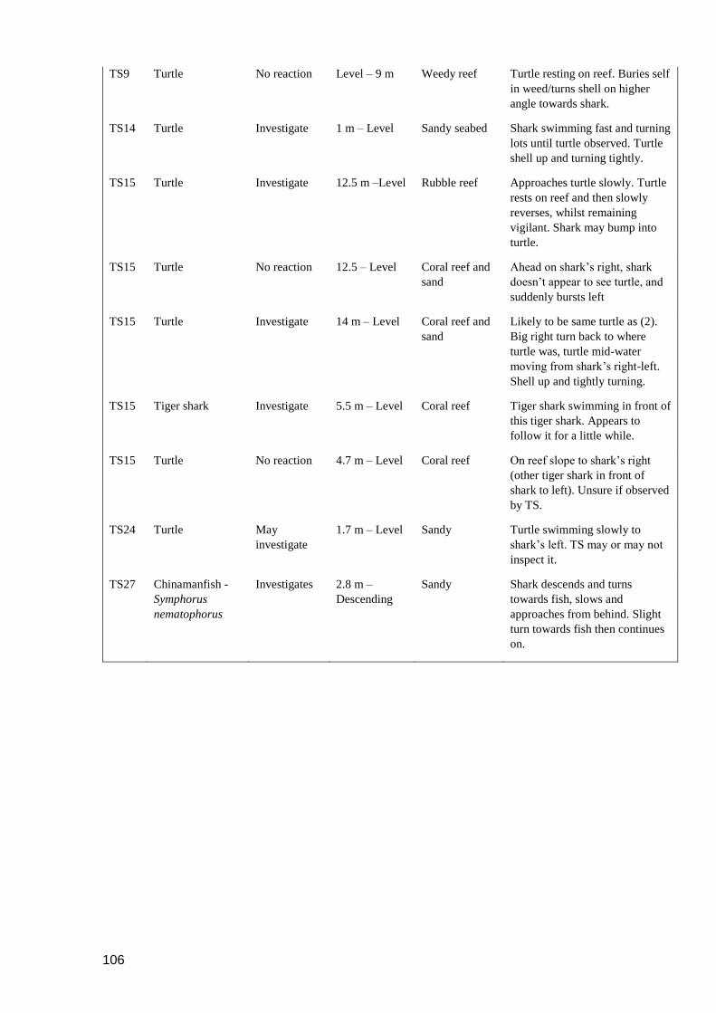
106
TS9 Turtle No reaction Level – 9 m Weedy reef Turtle resting on reef. Buries self
in weed/turns shell on higher
angle towards shark.
TS14 Turtle Investigate 1 m – Level Sandy seabed Shark swimming fast and turning
lots until turtle observed. Turtle
shell up and turning tightly.
TS15 Turtle Investigate 12.5 m –Level Rubble reef Approaches turtle slowly. Turtle
rests on reef and then slowly
reverses, whilst remaining
vigilant. Shark may bump into
turtle.
TS15 Turtle No reaction 12.5 – Level Coral reef and
sand
Ahead on shark’s right, shark
doesn’t appear to see turtle, and
suddenly bursts left
TS15 Turtle Investigate 14 m – Level Coral reef and
sand
Likely to be same turtle as (2).
Big right turn back to where
turtle was, turtle mid-water
moving from shark’s right-left.
Shell up and tightly turning.
TS15 Tiger shark Investigate 5.5 m – Level Coral reef Tiger shark swimming in front of
this tiger shark. Appears to
follow it for a little while.
TS15 Turtle No reaction 4.7 m – Level Coral reef On reef slope to shark’s right
(other tiger shark in front of
shark to left). Unsure if observed
by TS.
TS24 Turtle May
investigate
1.7 m – Level Sandy Turtle swimming slowly to
shark’s left. TS may or may not
inspect it.
TS27 Chinamanfish -
Symphorus
nematophorus
Investigates 2.8 m –
Descending
Sandy Shark descends and turns
towards fish, slows and
approaches from behind. Slight
turn towards fish then continues
on.

107
Chapter 5 Depth dependent dive kinematics
suggest cost-efficient foraging
strategies by tiger sharks
5.1 Abstract
Tiger sharks (Galeocerdo cuvier) are a keystone, top-order predator that are assumed to engage
in cost-efficient movement and foraging patterns. To investigate the extent to which patterns of
oscillatory diving by these animals conform to a strategy of cost-efficient foraging, we used a
biologging approach to model their cost of transport. High-resolution biologging tags were
deployed on 21 tiger sharks at Ningaloo Reef for durations of 5-48 hours. Tags recorded animal
depth, and through the use of accelerometers, in situ measurements of animal trajectory and
locomotion, which enabled calculation of dive geometry and swimming energetics. Using overall
dynamic body acceleration (ODBA) as a proxy for energy expenditure, we modelled the cost of
transport of oscillatory movements of varying geometries in both horizontal and vertical planes
for tiger sharks. The cost of horizontal transport was minimized at absolute dive angles greater
than 0°, so that oscillations conserved energy relative to swimming at a level depth. Optimization
of vertical travel occurred at steeper angles. The absolute dive angles of tiger sharks increased
between inshore and offshore zones, presumably to reduce energy costs while continuously
hunting for prey in both benthic and surface habitats. On shallow (<3 m depth) sandflats at
Ningaloo Reef, tiger sharks were able to hunt continuously while exploiting the most cost-
efficient dive angles. In deeper environments, steeper dive angles were found to partially
compensate for the added energy costs of transiting a longer distance through the water column
between the surface and the seafloor. Oscillatory movements of tiger sharks conform to strategies
of cost-efficient foraging, and shallow sandflats appear to be an important habitat for both hunting
prey and saving energy.
5.2 Introduction
The tiger shark is a top-order predator that has wide-ranging impacts on the ecology of the tropical
and warm-temperate marine ecosystems they inhabit (Heithaus et al. 2002b; Heithaus et al. 2007).
These sharks are generalist feeders with anatomical specializations for feeding on large prey
(Lowe et al. 1996; Heithaus 2001; Simpfendorfer et al. 2001; Hammerschlag et al. 2016; Ferreira
et al. 2017). Although they actively hunt prey, they are also facultative scavengers
(Hammerschlag et al. 2016), which avoids or reduces many of the energetic costs involved in the

108
process of predation (Clua et al. 2013; Hammerschlag et al. 2016). However, injured or dead prey
are windfalls that only occur sporadically and for the most part, tiger sharks must actively locate,
hunt and capture their food. Like all top-order predators, they are assumed to do so in a cost-
efficient manner (Ruxton and Houston 2004).
Tagging studies have revealed that the fine-scale movements of tiger sharks are characterised by
patterns of oscillatory ascents and descents (“dives”) throughout the water column (Heithaus et
al. 2002b; Nakamura et al. 2011; Chapter 4), a behaviour that is shared by many species of large
epipelagic fishes (see Chapter 2). For tiger sharks, these dives have been recorded in a number of
habitats, ranging from very shallow (<4 m) seagrass beds in Shark Bay (Heithaus et al. 2002b),
to deeper (>100 m), offshore waters in Hawaii and Brazil (Holland et al. 1999; Nakamura et al.
2011; Afonso and Hazin 2014). It has been argued that these oscillatory movements are not likely
to be primarily driven by behavioural thermoregulation, because they often occur in well-mixed
and/or shallow environments (Heithaus et al. 2002b; Nakamura et al. 2011) where there is little
gradient in temperature between the surface and the seafloor. Instead, previous studies have
suggested that oscillatory diving provides an effective search strategy for an animal that feeds on
prey both at the surface and near the seabed (Heithaus et al. 2002b; Nakamura et al. 2011). More
recently, tiger sharks tagged at Ningaloo Reef have been found to make oscillatory dives during
the tortuous movements associated with area-restricted search (see Chapter 4). These oscillatory
dives also occurred during directional swimming, suggesting that there may be drivers other than
foraging contributing to these patterns.
In addition to allowing sharks to search for prey, oscillatory dives may represent a strategy to
reduce the cost of transport. Weihs (1973) proposed that a two-stage mode of swimming may
allow negatively-buoyant animals to reduce energy expenditure relative to swimming at a level
depth between two horizontal points, whereby individuals oscillate through the water column,
gliding on descent and actively swimming on ascent. Recent advances in the use of tri-axial
sensors in biologging tags provide a means to test this hypothesis in a natural setting. Tri-axial
accelerometers can be used to calculate dive angles in addition to overall dynamic body
acceleration (ODBA), a parameter that can act as a proxy for energy consumption (Gleiss et al.
2011a), and can therefore be used to quantify and compare the energy costs of different movement
behaviours. Gleiss et al. (2011a) used a biologging approach to explore how differences in the
dive geometry in whale sharks (Rhincodon typus) influenced the cost of transport with respect to
both horizontal and vertical distance, using dynamic body acceleration as a proxy for power.
Empirical optimality models suggested that some dive profiles reduced the cost of horizontal
transport, while other steeper-angled dives minimized the cost of vertical transport; indicating
that the choice of dive undertaken by an individual may be dependent on the ecological context
i.e. travel, search or foraging (Gleiss et al. 2013). Collectively, whale sharks were found to use
oscillatory movements to conserve energy while both travelling and searching for prey,
109
culminating in the observed patterns of cost-efficient foraging.
As tiger sharks are negatively buoyant (Nakamura et al. 2011), we hypothesise that they may also
exploit their weight in water and use oscillatory movements to reduce the cost of transport while
travelling or searching for prey. However, given that dead prey will sink to the bottom whereas
active prey may be most easily ambushed at the surface where they can be approached from below
(Martin and Hammerschlag 2012) movement strategies may be habitat dependent. Tiger sharks
tagged at Ningaloo Reef were found to undertake oscillatory movements in both inshore and
offshore habitats (see Chapter 4). In very shallow habitats (<3 m), tiger sharks would have no
need to undergo vertical search patterns given the short distance between the surface of the water
and the seabed. In deeper habitats, however, individuals would need to actively transit through a
larger water column between the surface and seabed in their search for prey. We therefore predict
that the diving energetics and kinematics of these animals will be dependent on the depth of the
habitat being occupied, with deeper waters featuring steeper dive angles to allow for faster transit
times.
Here, we use a biologging approach to examine the energetics of oscillatory diving behaviour in
tiger sharks at Ningaloo Reef, Western Australia. We examine the incidence of gliding behaviour
in tiger sharks and model the cost of transport of oscillatory movements of varying movement
geometries using ODBA as a proxy for energy expenditure. We document the range of dive angles
utilised by tagged sharks, particularly in relation to habitat depth, discuss the role of oscillatory
movements in both efficient foraging and energy conservation, and re-evaluate the drivers of
oscillatory diving in this species.
5.3 Methods
5.3.1 Ethics
All methods were used in accordance with approved guidelines by the University of Western
Australia Animal Ethics Committee (RA/3/100/1437), and under permit numbers 2881 (WA
Department of Fisheries) and 08-000322-3 (WA Department of Parks and Wildlife).
5.3.2 Data collection
Tiger sharks were captured and tagged at Ningaloo Reef, Western Australia (Figure 6.1) in April
and May 2017 following the methods described in Chapter 5. In brief, biologging tags were
clamped to the dorsal fins of 22 captured tiger sharks for periods of 7-48 hours (see Table 4-2).
Tags were equipped with tri-axial accelerometers, magnetometers and gyroscopes, and sensors
for depth, temperature and light. All sensors recorded continuously at 20 Hz. In addition, 14 of
the 22 deployments recorded video at pre-programmed hours of the day for a maximum of six

110
hours per deployment. The tags detached from the clamp in the days following tagging, and were
recovered using a handheld VHF receiver operated from a vessel.
Figure 5.1. Location of tagging and tag recoveries. Note that eight tags are outside of the map area – two
approximately 10 km further north, and six offshore (ranging from 15-27 km offshore).
111
5.3.3 Data processing
Data recorded by the tags were processed to obtain a number of parameters classifying shark
movements, behaviour and the external environment. Vertical phases of movement, dive angles,
overall dynamic body acceleration (ODBA), and tailbeat kinematics were calculated as described
in Chapter 4. In brief, the depth record was split into vertical phases of ascent, descent and
constant depth. Tri-axial sensor data were then used to calculate the pitch angles of vertical
movements, ODBA, and the signal amplitude and frequency of tailbeats in Igor Pro ver. 7.0.4.1
(Wavemetrics, Inc. Lake Oswego, USA). Tailbeat data were used to calculate the recovery period
from capture following methods outlined by Whitney et al. (2016b). Video data were also
processed as per Chapter 4, and were used to record interactions with prey, determine habitat
types, and validate behaviours recorded by the sensors (e.g. tailbeats and gliding behaviour). In
addition, sensor data were used to compute gliding behaviour, and ascent and descent speed, as
described below.
5.3.3.1 Gliding behaviour
We used a continuous wavelet transformation on the dynamic component of the sway (i.e. lateral)
axis to calculate the signal amplitude and frequency of shark tailbeats using both the acceleration
and angular velocity data (Sakamoto et al. 2009). The resulting signals were compared to
determine the best measure of tailbeat activity. The angular velocity data produced the clearest
tailbeat signal, and were consequently used to quantify the incidence of gliding behaviour –
defined here as a cessation of tailbeats for more than one second – through a two-step process.
Gliding behaviour was firstly computed using the ‘k-means cluster’ function in the Ethographer
for Igor Pro (Sakamoto et al. 2009). This function clusters the spectra computed by the wavelet
transformation based on similarity of shape. The behavioural spectrum with the lowest peaks in
angular velocity signal amplitude was assumed to represent gliding behaviour (Nakamura et al.
2011), and the incidence of the resulting cluster was then inspected against the dynamic sway
data. As this cluster did not match with gliding behaviour in some individuals (i.e. tailbeats
evident in sway data were classified to be gliding, and vice versa), a mask was created using the
characteristics of the angular velocity signal amplitude and tailbeat frequency where the cluster
was judged to correctly classify gliding behaviour (from visual inspection of the dynamic sway
data and concurrent videos). This mask was then used to extract glides from all sharks. These
were confirmed by a visual scan of the data.
5.3.3.2 Ascent and descent speed
Vertical velocity (VV) and pitch were used to estimate the mean speed of ascents and descents
through trigonometry, however, this could only be calculated when pitch exceeded 20° due to
the large errors associated with estimating speed at low pitch angles (Gleiss et al. 2011b).

112
5.3.3.3 Window size and statistics
The sampling window used for analysis was determined in Chapter 4 by calculating the time
period for which the highest variance in turning angles was observed, while being of sufficient
size to capture the longest recorded dives in their entirety. This time window was estimated to be
15 minutes (900 seconds), and within this period, a number of vertical movement parameters were
summarized including mean (± standard deviation) and maximum depth, ascent pitch, descent
pitch, ascent VV and descent VV. The percent of time spent moving vertically (ascending and
descending), termed the ‘diving ratio’, was also calculated within each window for each
individual as per:
𝐷𝑖𝑣𝑖𝑛𝑔 𝑟𝑎𝑡𝑖𝑜 = 𝑇𝑖𝑚𝑒 𝑣𝑒𝑟𝑡𝑖𝑐𝑎𝑙𝑙𝑦 𝑚𝑜𝑣𝑖𝑛𝑔 𝑖𝑛 𝑤𝑖𝑛𝑑𝑜𝑤 (𝑠𝑒𝑐𝑜𝑛𝑑𝑠)
𝑇𝑜𝑡𝑎𝑙 𝑡𝑖𝑚𝑒 𝑖𝑛 𝑠𝑎𝑚𝑝𝑙𝑖𝑛𝑔 𝑤𝑖𝑛𝑑𝑜𝑤 (900 𝑠𝑒𝑐𝑜𝑛𝑑𝑠)
5.3.4 Data analysis
5.3.4.1 Generalised linear mixed models (GLMMs)
Generalised linear mixed models (GLMMs) were built using the nlme package in R 3.4.0
(Pinheiro et al. 2017; R Core Team 2017) to investigate possible relationships between seabed
depth and vertical movement behaviours in tiger sharks. The maximum depth (m) recorded within
each time window was used as a proxy for seabed depth (based on video analysis; see Chapter 4
Results and Figure S 4-2) and was set as the explanatory variable, and tiger shark identity set as
a random variable for all models. Ascent pitch, descent pitch, ascent VV, descent VV and diving
ratio were all set sequentially as response variables. We used the corAR1 function to account for
temporal auto-correlation in our datasets (Zuur et al. 2009). Together with nautical charts from
Ningaloo Reef, maximum depth was used to classify windows as either ‘inshore’ (<25 m, inside
the reef) or ‘offshore’ (>25 m, outside the reef). GLMMs were analysed separately for inshore
and offshore periods due to heterogeneity in residuals and an unbalanced design. The resulting
models were compared against the null models and ranked using Akaike’s information criterion
(AIC).
To investigate if observed changes in diving ratio with depth were an artifact of our selected
sampling window, we calculated diving ratio for oscillations occurring in increasingly deeper
water given a fixed interval of level swimming at the surface and seabed. One-hour long depth
traces were simulated for a hypothetical shark oscillating in depths of 5, 10, 20, 30, 40, 50 and 60
m. The ascent VV and descent VV for each depth zone were determined following relationships
calculated between VV and seabed depth (see above). The fixed interval spent at the surface and
on the seabed between vertical movements was set at two minutes following exploration of the
depth traces. Diving ratio was calculated for each of the four 15 minute windows, and averaged
for the hour so that one value of diving ratio was calculated for each depth.

113
5.3.4.2 Cost of transport models
We modelled the cost of transport of oscillatory movements of varying geometries in relation to
optimization of either horizontal or vertical distance travelled following methods similar to those
described by Gleiss et al. (2011a) (Figure 5.2). Firstly we calculated the total cost of an oscillation
(ascent (a) and descent (d) combined; TC) based on pitch angle (φ) and time taken (T) using the
equation:
TC = Ta(φa) × ODBA (φa) + Td (φd) × ODBA (φd) + k × (Td (φd) + Ta (φa))
ODBA was used to calculate energetic costs of a given dive angle. For ascents, this was calculated
from the relationship between ODBA and ascent angle (Figure 5.3a), and for descents a single
mean value (0.012) was used as no relationship was found between descent angle and ODBA
(Figure 5.3b). The proxy for basal cost in our model (k) was estimated from published figures to
be approximately 0.6 × routine metabolic rate, as estimated from a range of species of shark
irrespective of size (see Dowd et al. 2006 and references therein). As mean ODBA recorded for
all sharks was ~0.026 g we estimated k at 0.0156 g. The time spent ascending (Ta) and descending
(Td) are a function of ascent and descent pitch respectively, and the mean speed:
Ta =
𝐷𝑒𝑝𝑡ℎsin (φa)
mean ascent speed
Td =
𝐷𝑒𝑝𝑡ℎsin (φd)
mean descent speed
We used a fixed mean estimate of speed for both ascents (0.87 m/s) and descents (0.85 m/s) as no
relationship was found between speed and pitch angle. TC was calculated for fixed ascent angles
from 5° to 45°, binned in 5° increments. For each ascent angle, TC was calculated sequentially
for decent angles of 5° to 20°, binned in 5° increments.
We constructed two different models based on the cost of transport for tiger sharks when moving
horizontally (COTHD) and vertically (COTVD). These models calculated the cost of moving a unit
of horizontal (HD) and vertical distance (VD) respectively, and were used to determine the angles
that optimized the efficiency of transport on each of these scales for this species. The COTHD was
modelled by:
𝐶𝑂𝑇𝐻𝐷
= 𝑇𝐶
𝐻𝐷

114
Where horizontal distance was calculated as a function of trigonometry from ascent and descent
pitch using the equation:
𝐻𝐷 = 𝐷𝑒𝑝𝑡ℎ
tan(𝜑𝑑) +
𝐷𝑒𝑝𝑡ℎ
tan(𝜑𝑎)
The COTVD was modelled by:
𝐶𝑂𝑇𝑉𝐷
= 𝑇𝐶
2 × 𝐷𝑒𝑝𝑡ℎ
All model calculations used oscillations of 10 m depth, however, the resulting COT for horizontal
and vertical distance was the same regardless of depth.
Figure 5.2. Schematic representation of an oscillatory movement, and the distance parameters used in
calculating the cost of transport.
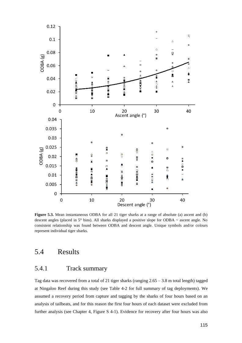
115
Figure 5.3. Mean instantaneous ODBA for all 21 tiger sharks at a range of absolute (a) ascent and (b)
descent angles (placed in 5° bins). All sharks displayed a positive slope for ODBA ~ ascent angle. No
consistent relationship was found between ODBA and descent angle. Unique symbols and/or colours
represent individual tiger sharks.
5.4 Results
5.4.1 Track summary
Tag data was recovered from a total of 21 tiger sharks (ranging 2.65 – 3.8 m total length) tagged
at Ningaloo Reef during this study (see Table 4-2 for full summary of tag deployments). We
assumed a recovery period from capture and tagging by the sharks of four hours based on an
analysis of tailbeats, and for this reason the first four hours of each dataset were excluded from
further analysis (see Chapter 4, Figure S 4-1). Evidence for recovery after four hours was also

116
provided by the video records, which showed investigation of prey and consumption of a
discarded fish head by sharks within two hours of release after tagging (Supplementary Video 1).
Tagged tiger sharks swam at a mean depth of 11.6 ± 17.5 m, predominately residing in inshore
habitats, with four tiger sharks moving into offshore habitats and one individual diving to a
maximum depth of 94 m. Sharks moved vertically for a mean of 38.4 ± 26% of their track and
utilised significantly steeper descent (-11.11 ± 3.6o) than ascent (9.38 ± 2.6o) angles (Wilcoxon
signed-ranks test, P < 0.001).
5.4.2 Gliding behaviour
There was a high level of individual variation in the proportion of gliding descents by tiger sharks
(range 0-35%, Figure 5.4). Six sharks glided for more than 19% of their total descent time, of
which three glided for more than 30% of their descents. A maximum uninterrupted glide time of
two minutes was recorded for one individual. Gliding was rarely recorded in the first four hours
of each tag deployment (designated as the recovery period) and no gliding behaviour was recorded
for two sharks (Figure 5.4). Gliding was exhibited by tiger sharks in both inshore and offshore
zones and occurred at a minimum descent angle of -8° and at a mean angle of -12.2 ± 2.7°.
5.4.3 Relationship between seabed depth and vertical
movement behaviours
GLMMs revealed significant relationships between seabed depth and vertical movements of tiger
sharks (Table 5-1). For inshore GLMMs, all models retained their predictor variables of vertical
movement, whereas for offshore models, only the random effect of tiger shark identity was
retained. Up to depths of 25 m (inshore) diving ratio, pitch and VV all increased with seabed
depth, after which point relationships plateaued and displayed high levels of variation (Figure S
5-1). Inshore, maximum/seabed depth explained 35% (marginal R2) of the variation in both diving
ratio and descent pitch. For all models, high conditional R2 values (up to 55%) suggested high
inter-individual variability in vertical movements (Table 5-1). Mean absolute pitch angles
increased between inshore and offshore habitats from 10.3 ± 2.8° to 14.1 ± 4.7° for descent, and
9 ± 2.3 to 10.7 ± 3.2° for ascent (Figure 5.5).
Between inshore and offshore habitats, the mean diving ratio increased from 31 ± 23% to 69 ±
17% (Figure 5.6a). From simulated depth data generated using VV from GLMM relationships
and fixed intervals of level swimming between vertical movements, diving ratios were found to
exhibit a similar pattern to that observed in the raw data (Figure 5.6). Despite VV also increasing
with depth, diving ratio increased quickly between 5 and 20 m depths, after which the slope
between subsequent points rapidly decreased.
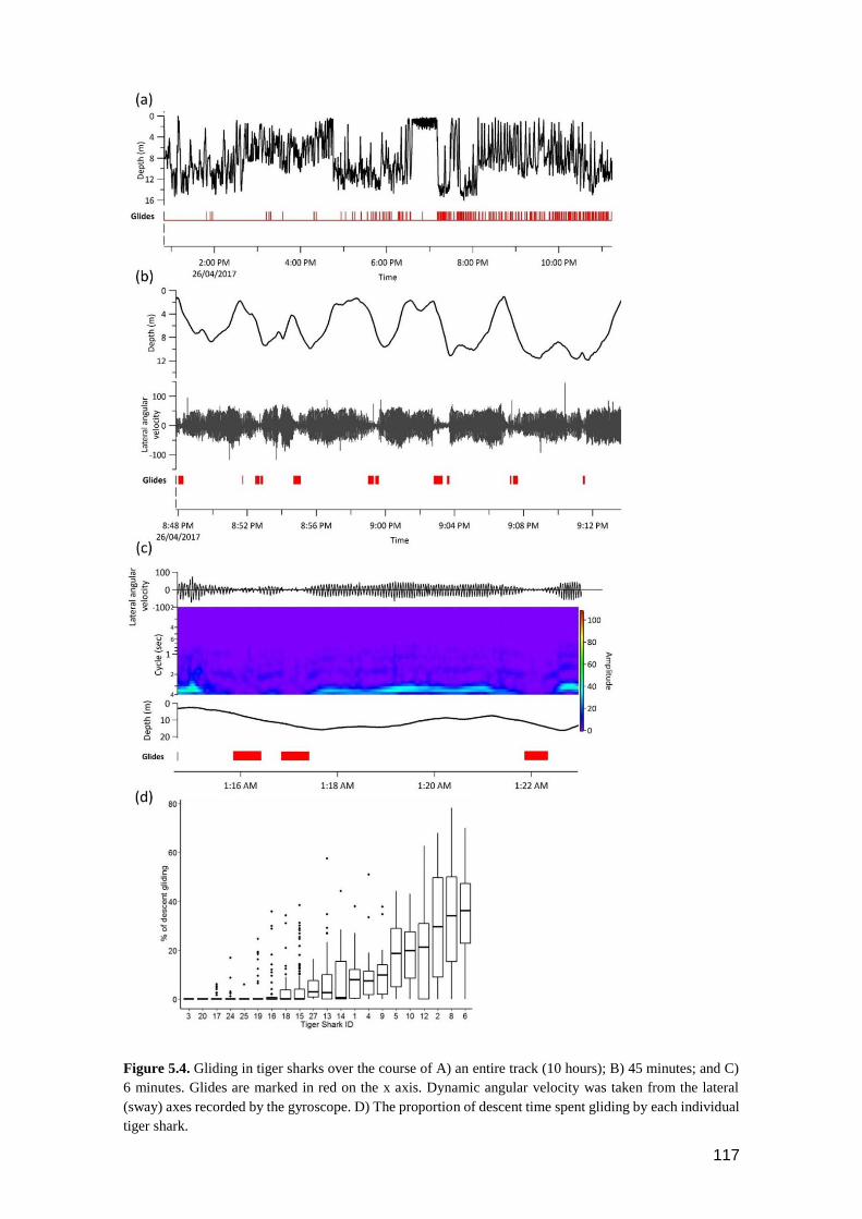
117
Figure 5.4. Gliding in tiger sharks over the course of A) an entire track (10 hours); B) 45 minutes; and C)
6 minutes. Glides are marked in red on the x axis. Dynamic angular velocity was taken from the lateral
(sway) axes recorded by the gyroscope. D) The proportion of descent time spent gliding by each individual
tiger shark.
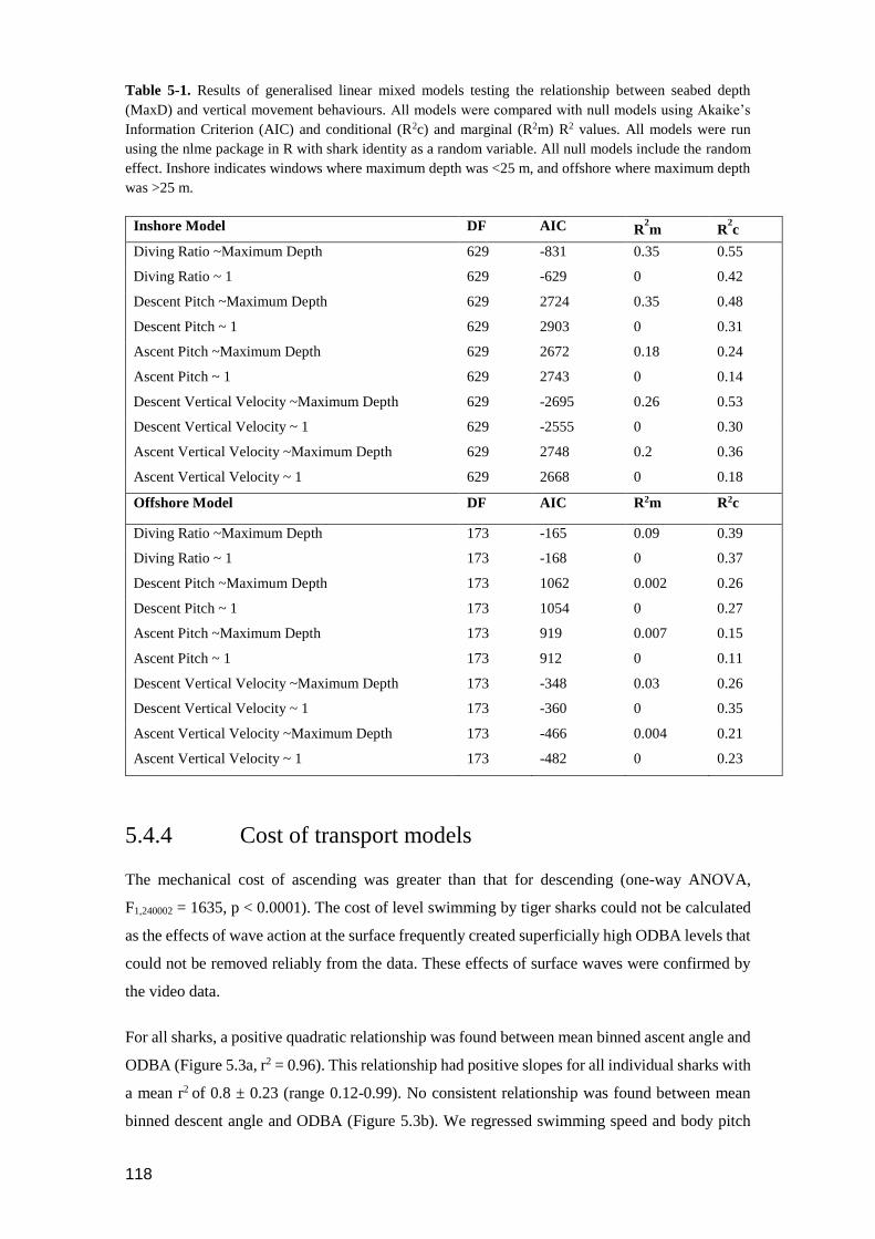
118
Table 5-1. Results of generalised linear mixed models testing the relationship between seabed depth
(MaxD) and vertical movement behaviours. All models were compared with null models using Akaike’s
Information Criterion (AIC) and conditional (R2c) and marginal (R2m) R2 values. All models were run
using the nlme package in R with shark identity as a random variable. All null models include the random
effect. Inshore indicates windows where maximum depth was <25 m, and offshore where maximum depth
was >25 m.
Inshore Model DF AIC R2m R
2c
Diving Ratio ~Maximum Depth 629 -831 0.35 0.55
Diving Ratio ~ 1 629 -629 0 0.42
Descent Pitch ~Maximum Depth 629 2724 0.35 0.48
Descent Pitch ~ 1 629 2903 0 0.31
Ascent Pitch ~Maximum Depth 629 2672 0.18 0.24
Ascent Pitch ~ 1 629 2743 0 0.14
Descent Vertical Velocity ~Maximum Depth 629 -2695 0.26 0.53
Descent Vertical Velocity ~ 1 629 -2555 0 0.30
Ascent Vertical Velocity ~Maximum Depth 629 2748 0.2 0.36
Ascent Vertical Velocity ~ 1 629 2668 0 0.18
Offshore Model DF AIC R2m R2c
Diving Ratio ~Maximum Depth 173 -165 0.09 0.39
Diving Ratio ~ 1 173 -168 0 0.37
Descent Pitch ~Maximum Depth 173 1062 0.002 0.26
Descent Pitch ~ 1 173 1054 0 0.27
Ascent Pitch ~Maximum Depth 173 919 0.007 0.15
Ascent Pitch ~ 1 173 912 0 0.11
Descent Vertical Velocity ~Maximum Depth 173 -348 0.03 0.26
Descent Vertical Velocity ~ 1 173 -360 0 0.35
Ascent Vertical Velocity ~Maximum Depth 173 -466 0.004 0.21
Ascent Vertical Velocity ~ 1 173 -482 0 0.23
5.4.4 Cost of transport models
The mechanical cost of ascending was greater than that for descending (one-way ANOVA,
F1,240002 = 1635, p < 0.0001). The cost of level swimming by tiger sharks could not be calculated
as the effects of wave action at the surface frequently created superficially high ODBA levels that
could not be removed reliably from the data. These effects of surface waves were confirmed by
the video data.
For all sharks, a positive quadratic relationship was found between mean binned ascent angle and
ODBA (Figure 5.3a, r2 = 0.96). This relationship had positive slopes for all individual sharks with
a mean r2 of 0.8 ± 0.23 (range 0.12-0.99). No consistent relationship was found between mean
binned descent angle and ODBA (Figure 5.3b). We regressed swimming speed and body pitch

119
where pitch was greater than 20° for each individual shark, and did not detect quantifiable changes
in speed with pitch angle (Table S 5.1). Where the relationship was found to be significant, slope
did not exceed 0.02, and we therefore concluded that increased locomotory activity at increasing
pitch was due to counteracting gravity, rather than increasing drag due to greater speed (Gleiss et
al. 2011b).
Figure 5.5. Relationship between dive angle and habitat depth. (a & b) Boxplots displaying differences in
ascent and descent pitch angle between habitat zones. Inshore denotes areas where maximum depth within
a window was <25 m, and offshore where depths were >25 m. Shark silhouettes angles are not to scale. (c
& d) Relationship between maximum depth in a sampling window and descent and ascent angle in inshore
zones (<25 m).
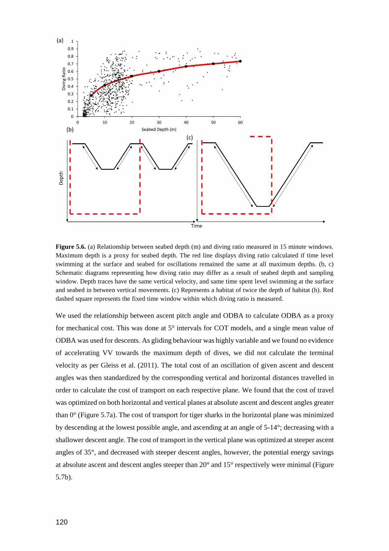
120
Figure 5.6. (a) Relationship between seabed depth (m) and diving ratio measured in 15 minute windows.
Maximum depth is a proxy for seabed depth. The red line displays diving ratio calculated if time level
swimming at the surface and seabed for oscillations remained the same at all maximum depths. (b, c)
Schematic diagrams representing how diving ratio may differ as a result of seabed depth and sampling
window. Depth traces have the same vertical velocity, and same time spent level swimming at the surface
and seabed in between vertical movements. (c) Represents a habitat of twice the depth of habitat (b). Red
dashed square represents the fixed time window within which diving ratio is measured.
We used the relationship between ascent pitch angle and ODBA to calculate ODBA as a proxy
for mechanical cost. This was done at 5° intervals for COT models, and a single mean value of
ODBA was used for descents. As gliding behaviour was highly variable and we found no evidence
of accelerating VV towards the maximum depth of dives, we did not calculate the terminal
velocity as per Gleiss et al. (2011). The total cost of an oscillation of given ascent and descent
angles was then standardized by the corresponding vertical and horizontal distances travelled in
order to calculate the cost of transport on each respective plane. We found that the cost of travel
was optimized on both horizontal and vertical planes at absolute ascent and descent angles greater
than 0° (Figure 5.7a). The cost of transport for tiger sharks in the horizontal plane was minimized
by descending at the lowest possible angle, and ascending at an angle of 5-14°; decreasing with a
shallower descent angle. The cost of transport in the vertical plane was optimized at steeper ascent
angles of 35°, and decreased with steeper descent angles, however, the potential energy savings
at absolute ascent and descent angles steeper than 20° and 15° respectively were minimal (Figure
5.7b).

121
5.5 Discussion
Our study provides evidence that oscillatory movements through the water column allowed tiger
sharks to conserve energy while travelling and searching for prey and resulted in a strategy of
cost-efficient foraging. Our empirical models of the cost of transport showed that, while in transit,
tiger sharks required less energy to move in oscillatory dives at shallow angles through the water
column than they did while swimming at a constant depth. Shallow angles of ascent and descent
allowed tiger sharks to reduce their COT in the horizontal plane, whereas steeper angles reduced
their energetic costs in the vertical plane. The absolute dive angles of tiger sharks increased
between inshore and offshore zones, presumably to reduce energy costs while continuously
hunting for prey in both benthic and surface habitats.
5.5.1 Cost of vertical movements
Patterns of gliding varied among tagged sharks. Gliding occurred through 0-35% of the overall
descent phase of oscillations for individuals at Ningaloo, a finding comparable to that of
Nakamura et al. (2011). Although the majority of sharks displayed increasing levels of gliding
behaviour post-release, as previously observed in black-tip sharks (Carcharhinus limbatus;
Whitney et al. 2016b), some sharks – including an individual tagged for >15 hours – recorded no
gliding behaviour throughout tag deployment. This variability may be driven by minor individual
differences in body composition (Adachi et al. 2014; Gleiss et al. 2017a), and/or behavioural
differences in their response to catch and release. At all spatial scales movements of tiger sharks
have been characterized by high levels of individual variation (Vaudo et al. 2014; Ferreira et al.
Figure 5.7. The cost of transport of a single oscillatory movement of a tiger shark on (a) a horizontal plane
and (b) a vertical plane. Arrows indicate where the cost of transport is minimised in both cases. Lines
represent the cost of a given descent pitch angle (label on figure) in relation to varying ascent pitch (x-axis).

122
2015).
The energetic costs involved in descents were significantly lower than those of ascent in tiger
sharks, despite the majority of the descent phases of oscillations involving active swimming. This
result is a factor of the negative buoyancy of these animals (Nakamura et al. 2011), as it would
enable their descent phase to be partially powered by gravity. When ascents and descents were
considered together, the cost of horizontal transport of this two-stage mode of swimming was
reduced at absolute angles greater than 0°, allowing tagged individuals to conserve energy relative
to the cost of swimming an equivalent horizontal distance at a level depth. The modelled cost of
horizontal transport for tiger sharks was minimized at a descent angle of -5° and ascent angle of
14°. This closely matches modelled dive angles of whale sharks, where horizontal transport was
optimized at -10° and 11° for descents and ascents, respectively (Gleiss et al. 2011b). For whale
sharks, costs were minimized at the smallest angle at which whale sharks could glide. Tiger sharks
displayed a minimal glide angle of -8°, and therefore we suspect that steeper optimal descent
angles may exist for individuals that display a greater degree of gliding behaviour. Optimization
of vertical travel for tagged tiger sharks also exhibited a similar patterns to whale sharks, whereby
steeper angles on ascent than descent reduced the cost of vertical transport. Ascent angles of 35°
were found to reduce the cost of vertical transport for tiger sharks at Ningaloo – a marked increase
from the 23° reported for whale sharks – although energy savings beyond 20° appear to be
minimal for tiger sharks (Gleiss et al. 2011b). The costs of vertical transport decreased with
increasingly steep descent angles, but again, energy savings beyond -15° appeared to be minimal.
5.5.2 Cost-efficient foraging
Oscillatory movements of tiger sharks have previously been thought to be a strategy to allow them
to alternate between searching the surface and seabed for prey (Heithaus et al. 2002b; Nakamura
et al. 2011). Heithaus et al. (2002b) found that tiger sharks often spend a short period of time
swimming at the surface before descending to swim along the seabed. After another short period
they ascend, presumably searching for prey at the surface during the time they reside there. These
patterns were consistent with those observed in our study. The diving ratio of tiger sharks tagged
at Ningaloo Reef increased as seabed depth increased i.e. sharks spent more time within a
sampling window ascending and descending relative to level swimming in deeper water. Upon
further examination of our data, however, we believed this pattern to be an artefact of our 15
minute sampling window. Larger distances needed to be traversed between the surface and seabed
in deeper water, meaning a greater proportion of time is spent vertically moving in these areas.
We therefore hypothesise that tiger sharks were in fact spending a similar length of time searching
the surface and benthos for prey in between oscillations, regardless of water depth (Figure 5.6).
In addition, ascent angles were shallower than descent angles and remained relatively constrained
between habitats. This may be a function of retinal specialization in the visual system of tiger

123
sharks (Bozzano and Collin 2000). Tiger sharks are able to observe their upper visual field in
greater detail (Bozzano and Collin 2000), and their angle of ascent may optimize the field of view
for searching for unsuspecting prey silhouetted above them.
In the shallowest, inshore waters (< 3 m), tiger sharks would be able to continuously hunt as either
the seabed or the surface would always remain within their field of view. Oscillatory behaviours,
however, continued in these habitats at very shallow dive angles, consistent with movements that
reduced the horizontal cost of transport. In addition, these movements occurred throughout both
directional travel and tortuous movements assumed to be associated with foraging behaviour
(Chapter 4), suggesting that foraging behaviour alone was not primarily driving these movements.
As tiger sharks moved into deeper waters, they would need to transit through a deeper water
column between surface and benthic habitats in their hunt for prey or to scavenge, reducing the
amount of time spent foraging and increasing the energy costs of this activity. Here, we found
that the dive angles used by tiger sharks at Ningaloo increased as these animals moved into deeper
waters, allowing them to compensate for the increased cost of hunting through a larger water
column. Collectively, vertical movements of the tagged tiger sharks culminated in patterns of
cost-efficient foraging.
5.5.3 Model limitations
The cost of transport models constructed here from tiger shark acceleration data incorporated
some parameters that do not allow for the accurate measurement of movement costs in this
species. Despite this, we believe that the overall model is relatively insensitive to errors, allowing
us to test our hypotheses regarding the cost-efficiency of tiger shark movements against the
qualitative predictions produced by the models. Errors are likely to occur in the estimate of basal
cost, as this has not specifically been calculated for tiger sharks, and in the estimates for speed,
as this was only calculated where absolute pitch angles exceeded 20°. Gleiss et al. (2011a) tested
the sensitivity of cost of transport models to predicting qualitative trends for whale sharks and
found that (1) both doubling and halving of basal cost had no appreciable change on optimal
ascent angle, and (2) variations in speed of 0.2 m/s either side of the mean descent speed only
changed optimal ascent angle by 2°. In addition, our speed estimates (0.85 m/s for descent and
0.87 m/s for ascent) fit into the range of those directly quantified by Nakamura et al. (2011)
(overall mean speed 0.54-0.92 m/s among individuals, 0.53-0.82 m/s when gliding). Therefore,
we believe model results accurately reflect the trends in dive pitch angles for optimizing the cost
of vertical and horizontal transport.
5.5.4 Seascape effects on energy expenditure and gain
Our results suggest that very shallow waters (<3 m) are the most cost-efficient place for tiger
sharks to forage, and may therefore represent an important energy landscape for these animals.

124
Variation in an energy landscape occurs where the cost of transport is influenced by physical
characteristics of the environment (Wilson et al. 2012). This results in animals modifying
movements among habitats to either exploit opportunities for energy gain, and/or reduce costs
(Shepard et al. 2013). Establishing the variability in movement costs across landscapes can help
us to understand how and why animals distribute themselves in space (Wilson et al. 2012). For
tiger sharks, alternating between the seabed and surface in the search for prey means that the
energetic costs of foraging increase with depth. Very shallow environments (<3 m), such as the
sandflats of Ningaloo Reef, represent a landscape where tiger sharks can move and forage at the
most cost-efficient dive angles. In addition, pseudo-tracks, video data and observations from the
ecotourism industry have highlighted the importance of the shallow sandflat environments for
tiger sharks at Ningaloo Reef (see Chapter 4). In these habitats, tiger sharks often displayed the
tortuous movement patterns thought to denote foraging behaviour (Kareiva and Odell 1987;
Adachi et al. 2017), and predator-prey interactions have frequently been observed here. Tiger
sharks tagged in other regions have also been found to display a preference for shallow habitats,
including seagrass habitats less than four meters in depth in Shark Bay, and lagoon habitats in
Hawaii (Heithaus et al. 2002b; Meyer et al. 2010).
The preferential selection of these shallow water habitats has implications for the distribution of
predation pressure, and therefore the distribution of prey species. A study conducted over 15 years
in the largely seagrass habitat of Shark Bay, Western Australia, found that the presence of tiger
sharks influenced the movements and behaviour of a number of prey species, including dolphins,
turtles and dugongs (Heithaus et al. 2012). Given the prolonged residency of tiger sharks at
Ningaloo Reef (several months) (Ferreira et al. 2015) it seems likely that they will have similar
structuring roles in these coral reef environments.
5.5.5 Conclusion
Collectively, our data showed that the oscillatory movements of coastal tiger sharks are the
product of a combined foraging and energy conservation strategy. Tiger sharks modified their
vertical movement behaviours between inshore and offshore zones, presumably to optimize the
use of energy while continuously hunting for benthic and air-breathing prey. The shallow
sandflats of Ningaloo Reef appear to be an important habitat for hunting prey and saving energy.
5.6 Acknowledgements
Fieldwork and tags were funded by crowdfunding on the Experiment platform (DOI:
10.18258/7190), a Holsworth Wildlife Research Endowment, a UWA Graduate Research School
fieldwork award and BigWave Productions. We thank Murdoch University and Coral Bay
Research Station for accommodation and vessel use while conducting fieldwork. This work

125
would not have been possible without the generous support of numerous volunteers, particularly:
Frazer McGregor, Abraham Sianipar, Adam Jolly, Blair Bentley, Evan Byrnes, Garry Teesdale
and Michael Tropiano providing valuable field support; Olivia Seeger and Abraham Sianipar who
helped with the video analysis. Nikolai Liebsch provided invaluable assistance with tag
functioning. Thanks to Lauren Peel for helpful comments on an earlier version of this manuscript.

126
5.7 Supplementary information
Supplementary Video 1: https://vimeo.com/303181061
Password: shark
Figure S 5-1. Relationships between dive angles and maximum depth; (a) Maximum depth and ascent
angle for all data. (b) Maximum depth and descent angle for all data only.

127
Table S 5.1. Estimated ascent and descent speeds calculated by pitch and vertical velocity for absolute dive
angles >20° for each individual tiger shark, and their relationship with pitch. Individuals with <20 points
were excluded (TS10, TS16, TS20, TS25). Note that where significant relationships exist, slopes do not
exceed an absolute value of 0.02.
Shark
ID
Vertical
phase
N Mean
speed
F-value P r2 Slope Intercept
TS1 Ascent 58 0.78 3.7 0.06 0.06 -0.01 1.04
Descent 540 0.79 0.41 0.52 0.008 <-0.001 -0.8
TS2 Ascent 181 0.87 1.70 0.19 0.009 -0.003 0.96
Descent 281 0.86 59.2 <0.001 0.17 -0.01 0.56
TS3 Ascent 24 0.79 17.1 <0.001 0.43 -0.008 0.99
Descent 88 0.87 3.6 0.06 0.04 -0.006 0.71
TS4 Ascent 215 0.91 8.8 0.003 0.04 0.01 0.59
Descent 315 0.90 10.36 0.001 0.03 -0.018 0.45
TS5 Ascent 504 0.97 5.8 0.02 0.01 0.004 0.87
Descent 979 0.82 21.59 <0.001 0.02 -0.003 0.75
TS6 Ascent 85 0.72 34.6 <0.001 0.3 0.009 0.49
Descent 456 0.58 41.02 <0.001 0.08 -0.007 0.41
TS8 Ascent 294 0.89 6.24 0.01 0.02 0.004 0.77
Descent 716 0.69 72.3 0.001 0.09 -0.01 0.40
TS9 Ascent 858 1.03 38.87 <0.001 0.04 0.004 0.92
Descent 1580 1.0 3157 0.001 0.67 -0.02 0.43
TS12 Ascent 50 0.65 2.1 0.155 0.04 -0.002 0.71
Descent 112 0.70 0.001 0.97 <0.001 -0.0001 0.69
TS13 Ascent 2041 0.92 3.93 0.05 0.002 -0.0007 0.94
Descent 3439 0.96 2455 0.001 0.42 0.02 0.4
TS14 Ascent 216 0.91 0.06 0.81 0.0003 -0.0007 0.92
Descent 301 0.83 0.17 0.68 0.0005 -0.002 0.79
TS15 Ascent 1149 0.74 9.5 0.002 0.008 0.002 0.67
Descent 1362 0.76 181.6 <0.001 0.12 -0.009 0.53
TS17 Ascent 127 0.98 0.52 0.47 0.004 0.002 0.94
Descent 663 0.96 46.2 <0.001 0.07 -0.02 0.56
TS18 Ascent 1059 1.25 11.48 <0.001 0.01 -0.003 1.3
Descent 3115 1.1 373.6 <0.001 0.11 -0.01 0.84
TS19 Ascent 101 0.90 13.02 <0.001 0.12 0.01 0.62
Descent 78 0.73 5.57 0.02 0.07 -0.005 0.60
TS24 Ascent 63 0.98 1.8 0.18 0.03 0.01 0.67
Descent 263 0.89 15.4 <0.001 0.06 -0.005 0.75
TS27 Ascent 958 0.76 26.3 <0.001 0.03 0.004 0.66
Descent 118 1.03 49.4 <0.001 0.31 -0.02 0.21

128
Chapter 6 First insight into the fine-scale
movement behaviours of sandbar
sharks Carcharhinus plumbeus
6.1 Abstract
The expanding use of biologging tags in studies of shark movement provides an opportunity to
compare fine-scale movement behaviours among species. In May 2017, we deployed high-
resolution biologging tags on four mature female sandbar sharks Carcharhinus plumbeus at
Ningaloo Reef for durations ranging between 13 and 25.5 hours. Pressure and tri-axial motion
sensors within these tags enabled the calculation of dive geometry, swimming kinematics and
path tortuosity at fine spatial scales (m-km) and concurrent validation of these behaviours from
video recordings. Sandbar sharks oscillated through the water column at shallow dive angles, with
gliding behaviour observed in the descent phase for all sharks. Continual V-shaped oscillatory
movements were occasionally interspersed by U-shaped dives that predominately occurred
around dusk. The bottom phase of these U-shaped dives likely occurred on the seabed, with dead-
reckoning revealing a highly tortuous, circling track. By combining these fine-scale behavioural
observations with existing ecological knowledge of sandbar habitat and diet, we argue that this
circling behaviour is likely to be a strategy for hunting benthic prey. Comparing dive geometry
and energetics with those of other sharks reveals common patterns in energetically efficient
oscillatory swimming.
6.2 Introduction
An understanding of the movement ecology of marine megafauna requires investigation of
patterns at a range of spatial and temporal scales across an individual’s lifetime (Nathan et al.
2008). Broad-scale movements determined by acoustic and satellite tracking can reveal migratory
pathways, environmental preferences and patterns in habitat use and residency (Braccini et al.
2017; Ferreira et al. 2019). Fine-scale movements recorded by advanced biologging tags allow
the quantification of patterns in activity, feeding and energetics (e.g. Gleiss et al. 2013;
Brownscombe et al. 2014; Brewster et al. 2018), and can provide behavioural and physiological
context to other studies of broad-scale movements (Whitney et al. 2012; 2019).
Recent biologging studies on whale sharks (Rhincodon typus) and oceanic whitetip sharks
(Carcharhinus longimanus) have shown that the foraging, energetics and movement patterns of
sharks are likely linked through behaviours that minimize energy outputs, while maximizing
foraging opportunities (cost-efficient foraging) (Gleiss et al. 2011b; Meekan et al. 2015;

129
Papastamatiou et al. 2018a). To date, the applicability of this concept to other sharks is difficult
to determine, as relatively few species have been studied using a biologging approach.
Here, we used biologging tags to investigate the fine-scale movement behaviours of adult sandbar
sharks (Carcharhinus plumbeus) for the first time. This species is globally distributed in tropical
and warm temperate coastal waters, and is commercially important throughout its range
(McAuley et al. 2007; Ebert et al. 2013). K-selected species traits, such as low fecundity and late
age at maturity, targeted fishing and predicted population declines have led to the sandbar shark
being listed as Vulnerable on the IUCN Red List (Musick et al. 2009). Largely because of its
commercial importance, there exists a robust understanding of the broad-scale (10-1000 km)
distribution, movements and diet of the species (Stevens and McLoughlin 1991; McElroy et al.
2006; Ellis and Musick 2007; Grubbs et al. 2007; McAuley et al. 2007; Barnes et al. 2016;
Braccini 2017; Braccini et al. 2017). Tracking studies have found that sandbar sharks are
generally wide-ranging, undergo large migrations (>1000 km) but also display evidence of site-
fidelity (Grubbs et al. 2007; Papastamatiou et al. 2010; Barnes et al. 2016; Braccini et al. 2017).
Diet studies in a number of regions have found a preference for feeding on benthic prey,
predominately demersal fishes, cephalopods and crustaceans (Cliff et al. 1988; Stevens and
McLoughlin 1991; McElroy et al. 2006; Ellis and Musick 2007). Our use of biologging tags
allowed our study to record fine spatial and temporal scale (m and seconds) behaviour that linked
foraging to movement. Our aim was to determine the extent to which these movements conformed
to patterns of cost-efficient foraging seen in other species monitored with this type of technology.
Patterns consistent across species support the contention that this type of foraging is a key
determinant of the vertical movements of sharks and other megafauna in marine environments.
6.3 Materials and methods
6.3.1 Data collection
In Western Australia, mature sandbar sharks are predominately found in north and north-west
tropical waters (McAuley et al. 2007; Braccini and Taylor 2016), and some degree of site fidelity
have been revealed around Ningaloo Reef (Figure 6.1a) (Braccini et al. 2017). We captured
sandbar sharks at this locality using baited drumlines inside the reef lagoon (22.99°S, 113.8°E) in
May 2017 (Figure 6.1a). Drumlines were equipped with a single 20/0 circle hook baited with fish
scraps. Three drumlines were deployed approximately 100 m apart at depths of 8-12 m between
7:00 and 16:00, and were monitored continuously. Once a shark was caught, it was secured
alongside a 5.8 m vessel by the leader of the fishing line and a tail rope. Each shark was measured
and its sex recorded before a biologging tag was clamped to the base of its dorsal fin.
Either a CATS Diary Tag (Customised Animal Tracking Solutions, Australia) or CATS Cam Tag

130
was deployed on sandbar sharks (Figure 6.1b, Figure 6.1c). Both are equipped with tri-axial
accelerometers, magnetometers and gyroscopes, depth, temperature and light sensors In addition,
the Cam tag housed a HD video camera, and speed sensors were present, but not functional, in
the diary tags. Active sensors recorded all parameters at 20 Hz, and video recorded at pre-
programmed hours of the day. CATS tags were attached to a stainless steel spring clamp [CATS,
Australia, (Gleiss et al. 2009b; Chapple et al. 2015)] via docking pin and a corrodible galvanic
timed release (GTR, Ocean Appliances, Australia) allowing the tags to be rigidly attached to the
dorsal fin. The GTRs were designed to dissolve in seawater after 24 hours. After this time the tag
would release from the clamp and float to the surface. Floating tag packages were tracked down
in the days following tagging using a hand-held VHF receiver operated from the vessel (Lear and
Whitney 2016). The magnesium sleeve on the clamp also dissolved after seven days, detaching
the clamp from the shark.
Figure 6.1. Tagged sandbar sharks at Ningaloo Reef. (a) Location of tag deployments (b) CATS
Cam tag clamped to the dorsal fin. (c) CATS Diary tag clamped to the dorsal fin.

131
6.3.2 Data processing
6.3.2.1 Depth Record
Zero offset corrections were applied to the depth record based on times when sharks were being
tagged at the surface. The depth record was then split into vertical swimming phases (‘ascending’,
’descending’ and ‘level swimming’) using vertical velocity (VV). To do this the depth record was
firstly smoothed using a ten second running mean and the average VV was calculated by taking
the difference of this smoothed depth between successive points at one second intervals. Ascents
and descents were defined where VV exceeded an absolute value of 0.05 m/s for more than ten
seconds, and level where this value was not exceeded (Whitney et al. 2016b).
6.3.2.2 Tri-axial sensor data
Data recorded by the accelerometer (acceleration) and gyroscope (angular velocity) were analysed
using Igor Pro ver. 7.0.4.1 (Wavemetrics, Inc. Lake Oswego, USA) and Ethographer (Sakamoto
et al. 2009). The gravitational component of acceleration (static acceleration) was determined
using a three second box smoothing window on the raw acceleration data (Shepard et al. 2008).
Shark body pitch angles (orientation of the shark with regard to the horizontal plane) were derived
by calculating the arcsine of the static acceleration in the surging (posterior-anterior) axis. To
correct for the tag attachment angle on each individual shark, we determined the pitch when the
shark was swimming at a constant depth (when VV was equal to zero), and subtracted this value
from all pitch estimates (Kawatsu et al. 2009). The dynamic component of acceleration was
calculated by subtracting the gravitational component from the raw acceleration for each axis. We
then used a continuous wavelet transformation on the dynamic component of the sway (lateral)
axis to calculate the acceleration signal amplitude and frequency of tailbeats. Using these same
methods, amplitude and frequency were calculated using the angular velocity data, and the
resulting signals were compared with those derived from the acceleration data to determine the
best measure of tailbeat kinematics.
The angular velocity data produced the clearest tailbeat signal and consequently was used to
quantify the incidence of gliding behaviour (cessation of tailbeats for more than one second) using
a combination of two methods. Gliding behaviour was firstly computed using the k-means cluster
function in Ethographer. This algorithm clusters the spectra computed by the wavelet
transformation based on similarity of shape. The behavioural spectrum with the lowest peaks in
amplitude was assumed to represent gliding behaviour (Nakamura et al. 2011). The incidence of
the resulting cluster was then inspected against the dynamic sway data. As this cluster did not
match with gliding behaviour in some individuals (i.e. tailbeats evident in sway data classified to
be gliding and vice versa), a mask was created using the characteristics of the tailbeat amplitude
and frequency where the cluster was judged to correctly classify gliding behaviour (from visual

132
inspection of the dynamic sway and concurrent videos). This mask was then used to extract glides
from all sharks, and an additional manual quality control was undergone in the case where the
mask obviously misclassified glides.
Tailbeat signals were also examined for evidence of a recovery period following the stress of
capture following Whitney et al. (2016b).
6.3.2.3 Shark heading and pseudo-track calculation
Acceleration and magnetometer data were used to calculate head yaw angle (hereafter referred to
as ‘heading’) and pseudo-tracks in the software Framework 4 (Walker et al. 2015; Whitney et al.
2019). Heading calculations required input of orientation of the sensors in the tags, and
magnetometer and acceleration data. The orientation of the device was corrected using orientation
specifications provided by CATS (N. Liebsch pers. comm). Pitch and roll calculated from the
accelerometer data were used to correct for tilt (Walker et al. 2015). In addition to the calculations
applied by Framework 4, we applied a three second box smoothing window to the heading data
to filter out the dynamic movements of the sharks caused by tail beating that created significant
yaw.
Heading was then used to calculate pseudo-tracks for each shark using dead-reckoning (Mitani et
al. 2003; Wilson et al. 2007). These calculations operate under the principle that the heading and
speed of an individual at time ‘t’ can be used to calculate the position at time ‘t+1’ (Walker et al.
2015). Because a fixed value of speed is unlikely to be representative of individual sharks, the
dead-reckoning will accumulate errors over the course of the track. Therefore, tracks were used
only for plotting short-term movements of the sharks in three-dimensional space (‘pseudo-tracks’)
and could not be used to estimate geographical positions (Wilson et al. 2007; Walker et al. 2015).
Heading data were also used to calculate the turning angles of individuals on a second-by-second
basis. Data were resampled to a one second frequency and converted to a 0-360° scale. The
minimum difference in angle between consecutive observations was used to determine turning
angle.
6.3.2.4 Window size and statistics
The time window used for analysis was selected by determining the window for which the highest
variance in turning angle was observed. This time window was estimated to be 15 minutes (900
seconds), and within this period, a number of vertical movement parameters were summarized
including mean and maximum depth, ascent pitch, descent pitch, ascent VV and descent VV. The
proportion of time spent moving vertically (ascending and descending), termed the ‘diving ratio’,
was also calculated for each window as per:

133
𝐷𝑖𝑣𝑖𝑛𝑔 𝑟𝑎𝑡𝑖𝑜 =𝑇𝑖𝑚𝑒 𝑣𝑒𝑟𝑡𝑖𝑐𝑎𝑙𝑙𝑦 𝑚𝑜𝑣𝑖𝑛𝑔 𝑖𝑛 𝑤𝑖𝑛𝑑𝑜𝑤 (𝑠𝑒𝑐𝑜𝑛𝑑𝑠)
𝑇𝑜𝑡𝑎𝑙 𝑡𝑖𝑚𝑒 𝑖𝑛 𝑠𝑎𝑚𝑝𝑙𝑖𝑛𝑔 𝑤𝑖𝑛𝑑𝑜𝑤
This parameter allowed us to discriminate between sampling windows where vertical movements
consisted of continuous oscillations through the water column or extended periods of level
swimming between dives. In addition, heading data were used to calculate measurements of path
tortuosity and direction. Firstly, turning angles were summed for each window to obtain an
estimate of tortuosity. This was also separately calculated for each vertical phase (level
swimming, ascending and descending), and standardized by the time spent in the relative phase
within a sampling window (i.e. the mean). Secondly, the Circular package in R was used to
calculate the mean resultant length, or 𝑅 of the heading, a measure of the concentration of
unimodal circular data (Pewsey et al. 2013). When 𝑅 is close to or equal to one, points are closely
clustered around the mean direction and are highly directional, and as 𝑅 approaches zero, points
spread more evenly in a circle and become tortuous.
6.3.2.5 Video analysis
Video recorded by the tags was analysed in BORIS (Behavioural Observation Research
Interactive Software; Friard and Gamba 2016). This open-source software allows the user to set
an ethogram and record the timing of these events. We set an ethogram to mark burst swimming
events, presence of seabed in the field of view, habitat type, and other notable behaviours. Video
was also used to validate parameters recorded and calculated from the tri-axial sensor data, such
as tailbeat frequency, bursts and glides.
6.3.3 Statistical analysis
To investigate if changes in vertical movements were related to changes in horizontal movements,
we constructed a series of generalized linear models (GLMs) for each individual sandbar shark
(N=4). Diving ratio within a sampling window (see 2.2.4) was set as the response variable in all
models, and turning (a proxy for tortuosity) as the explanatory variable. The first set of models
used summed turning angles to explore the general relationship between tortuosity and diving
behaviour in tagged sharks. For the remaining models, mean turning angle for each phase of
vertical movement (level swimming, ascent and descent, see 2.2.4) was sequentially set as the
explanatory variable. Inspection for correlation at lag = 1 found no serial correlation in the data.
Statistical analysis was performed in R 3.4.0 (R Core Team 2017).

134
6.4 Results
Four mature female sandbar sharks ranging in length from 1.76 – 1.89 m TL were caught and
tagged at Ningaloo Reef in May 2017 (two camera tag and two diary tag deployments, Table 6-1).
Time from capture to release did not exceed 25 minutes for any of the tagged sharks. All deployed
tags were recovered after a mean attachment duration of 18 hours (range 13-25.5 hours). All
sensors recorded continuously for all four tag deployments, excluding the video camera, which
only recorded a total 5.5 hours and 30 minutes in two deployments.
The quantification of the post-release recovery period for sandbar sharks using tailbeat data was
confounded by the immediate movement into deeper water by three of the tagged individuals
(Figure S 6-1). For these sharks, increases in tailbeat frequency were associated with deeper dives.
Shark 4 remained inshore and no recovery period was observed i.e. there was no apparent effect
of capture on activity (Figure S 6-1). As a result, the entire recorded track from shark release to
tag detachment for each individual was used in the analysis.
6.4.1 Vertical movements
Tagged sandbar sharks swam at a mean depth of 23.4 ± 17.5 m, reaching a maximum depth of
96.6 m (Table 6-2). Sharks moved vertically in an oscillating pattern for a mean 57 ± 17.6% of
their track at a mean ascent angle of 11.4 ± 2.2° and descent angle of -11.5 ± 3.5° (Table 6-2).
Sharks displayed a mean tailbeat frequency of 0.65 ± 0.19 Hz, averaging 0.72 ± 0.12 Hz on ascent
and 0.57 ± 0.13 Hz on descent. Gliding behaviour was observed throughout 13.2 ± 14.3% of the
descent phase (range 0-75%), with a maximum continuous glide time of 210 seconds (Figure 6.2,
Table 6-2). Sparse tailbeats often interrupted glides during descents (Figure 6.2). For other
summary statistics of vertical movements, see Table 6-2.
The depth record for each shark consisted of continual V-shaped oscillatory vertical movements,
interspersed by occasional U-shaped dives with extended bottom periods (Figure 6.3). These U-
shaped dives occurred predominately around dusk for all individuals. Through a combination of
seabed observations in the video, dead-reckoning and the gradual increase in window maximum
depth as three sharks moved offshore, we assumed that the oscillations were limited vertically by
the seabed. Comparing these maximum depths with bathymetry of the study site, three sharks
moved offshore (maximum depths >70 m), and one shark appeared to remain inside the reef
(Shark 4, maximum depth <20 m).
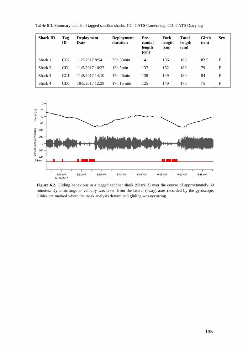
135
Table 6-1. Summary details of tagged sandbar sharks. CC: CATS Camera tag, CD: CATS Diary tag
Shark ID Tag
ID
Deployment
Date
Deployment
duration
Pre-
caudal
length
(cm)
Fork
length
(cm)
Total
length
(cm)
Girth
(cm)
Sex
Shark 1 CC2 11/5/2017 8:54 25h 33min 141 156 185 82.5 F
Shark 2 CD1 11/5/2017 10:27 13h 5min 137 152 189 79 F
Shark 3 CC1 11/5/2017 14:10 17h 46min 138 149 180 84 F
Shark 4 CD1 18/5/2017 12:29 17h 15 min 125 140 176 75 F
Figure 6.2. Gliding behaviour in a tagged sandbar shark (Shark 3) over the course of approximately 30
minutes. Dynamic angular velocity was taken from the lateral (sway) axes recorded by the gyroscope.
Glides are marked where the mask analysis determined gliding was occurring.
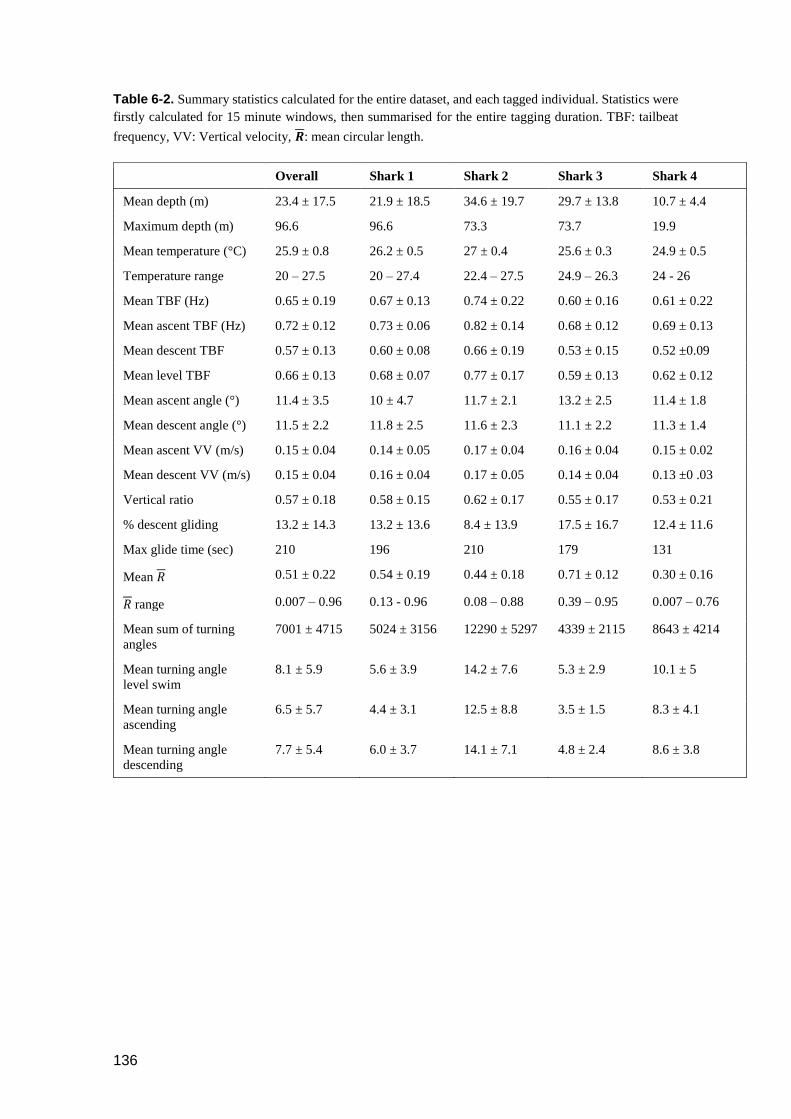
136
Table 6-2. Summary statistics calculated for the entire dataset, and each tagged individual. Statistics were
firstly calculated for 15 minute windows, then summarised for the entire tagging duration. TBF: tailbeat
frequency, VV: Vertical velocity, 𝑹: mean circular length.
Overall Shark 1 Shark 2 Shark 3 Shark 4
Mean depth (m) 23.4 ± 17.5 21.9 ± 18.5 34.6 ± 19.7 29.7 ± 13.8 10.7 ± 4.4
Maximum depth (m) 96.6 96.6 73.3 73.7 19.9
Mean temperature (°C) 25.9 ± 0.8 26.2 ± 0.5 27 ± 0.4 25.6 ± 0.3 24.9 ± 0.5
Temperature range 20 – 27.5 20 – 27.4 22.4 – 27.5 24.9 – 26.3 24 - 26
Mean TBF (Hz) 0.65 ± 0.19 0.67 ± 0.13 0.74 ± 0.22 0.60 ± 0.16 0.61 ± 0.22
Mean ascent TBF (Hz) 0.72 ± 0.12 0.73 ± 0.06 0.82 ± 0.14 0.68 ± 0.12 0.69 ± 0.13
Mean descent TBF 0.57 ± 0.13 0.60 ± 0.08 0.66 ± 0.19 0.53 ± 0.15 0.52 ±0.09
Mean level TBF 0.66 ± 0.13 0.68 ± 0.07 0.77 ± 0.17 0.59 ± 0.13 0.62 ± 0.12
Mean ascent angle (°) 11.4 ± 3.5 10 ± 4.7 11.7 ± 2.1 13.2 ± 2.5 11.4 ± 1.8
Mean descent angle (°) 11.5 ± 2.2 11.8 ± 2.5 11.6 ± 2.3 11.1 ± 2.2 11.3 ± 1.4
Mean ascent VV (m/s) 0.15 ± 0.04 0.14 ± 0.05 0.17 ± 0.04 0.16 ± 0.04 0.15 ± 0.02
Mean descent VV (m/s) 0.15 ± 0.04 0.16 ± 0.04 0.17 ± 0.05 0.14 ± 0.04 0.13 ±0 .03
Vertical ratio 0.57 ± 0.18 0.58 ± 0.15 0.62 ± 0.17 0.55 ± 0.17 0.53 ± 0.21
% descent gliding 13.2 ± 14.3 13.2 ± 13.6 8.4 ± 13.9 17.5 ± 16.7 12.4 ± 11.6
Max glide time (sec) 210 196 210 179 131
Mean 𝑅 0.51 ± 0.22 0.54 ± 0.19 0.44 ± 0.18 0.71 ± 0.12 0.30 ± 0.16
𝑅 range 0.007 – 0.96 0.13 - 0.96 0.08 – 0.88 0.39 – 0.95 0.007 – 0.76
Mean sum of turning
angles
7001 ± 4715 5024 ± 3156 12290 ± 5297 4339 ± 2115 8643 ± 4214
Mean turning angle
level swim
8.1 ± 5.9 5.6 ± 3.9 14.2 ± 7.6 5.3 ± 2.9 10.1 ± 5
Mean turning angle
ascending
6.5 ± 5.7 4.4 ± 3.1 12.5 ± 8.8 3.5 ± 1.5 8.3 ± 4.1
Mean turning angle
descending
7.7 ± 5.4 6.0 ± 3.7 14.1 ± 7.1 4.8 ± 2.4 8.6 ± 3.8

137
Figure 6.3. Entire depth record and gliding behaviour for each tagged sandbar shark. Glides are marked where the
mask analysis determined gliding was occurring. Dashed blue squares denote extended periods of U-shaped diving,
and associated looping behaviour. (a) Shark 1; (b) Shark 2; (c) Shark 3; and (d) Shark 4. Note that both x- and y-
axes scales differ between sharks.

138
6.4.2 Tortuosity and three-dimensional paths
All sharks displayed periods of both directional and tortuous travel, with an overall mean 𝑅 of
0.51 ± 0.22 (range among individuals 0.007 – 0.96, Table 6-3). The GLMs revealed a significant
negative relationship between tortuosity and diving ratio for three of the four individual sharks,
with turning explaining 53-66% of the variation in diving ratio (Table 6-3, Figure S 6-2). Shark
2 showed no significant relationship between tortuosity and diving ratio, with this individual
observed to display relatively high levels of tortuosity throughout the track in comparison to the
other sharks (Table 6-1). Further investigation of the windows with the highest tortuosity (high
sum of turning angles and low 𝑅), found tortuous windows to be associated with U-shaped dives
(Figure 6.4). Due to extended periods of level swimming, the diving ratio was relatively low in
sampling windows containing U-shaped dives. For all tagged sharks, pseudo-tracks displayed
repeated circling on the bottom phase of these dives, irrespective of depth (Figure 6.5). For
example, U-shaped dives recorded throughout dusk periods had circling phases at depths of 36.5,
67, 67 and 14.6 m for each individual shark respectively (Figure 6.5). These bottom phases lasted
a maximum of 55 minutes.
As sampling windows of low or high diving ratio represented U- or V-shaped dives respectively,
models were taken a step further to investigate changes in turning angle for each phase of vertical
movement. Significant negative relationships were revealed between diving ratio and turning
angles for both level and ascent phases in Sharks 1, 3 and 4 (Table S 6.1). The relationship was
stronger for level swimming phases (R2 = 0.32-0.42) than ascent phases (R2 = 0.12-0.19). More
tortuous ascents were evident in U-shaped dives, and directional ascents in V-shaped dives
(Figure 6.6). No relationship was found between descent turning angles and diving ratio, and
similar patterns of descent were found in both V- and U-shaped dives (e.g. Figure 6.6).
Table 6-3. Linear model comparisons using Akaike’s Information Criterion (AIC), R2, and p-values. ΔAIC
displays deviance in AIC scores from null model. Diving ratio is modelled as a function of turning, where
turning is the sum of the turning angles for a sampling window. Model results where turning is standardised
by vertical phase of movement are shown in Supplementary Table 1.
Shark ID Model df Slope AIC ΔAIC R2 p
Shark 1 Diving ratio ~ turning
Diving ratio ~ 1
101
102
-0.03 -169
-91
-66 0.54 <0.001
Shark 2 Diving ratio ~ turning
Diving ratio ~ 1
51
52
-0.006 -37
-36
-1 0.04 0.15
Shark 3 Diving Ratio ~ turning
Diving ratio ~ 1
70
71
-0.05 -97
-44
-53 0.53 <0.001
Shark 4 Diving Ratio ~ turning
Diving ratio ~ 1
68
69
-0.03 -93
-18
-75 0.66 <0.001
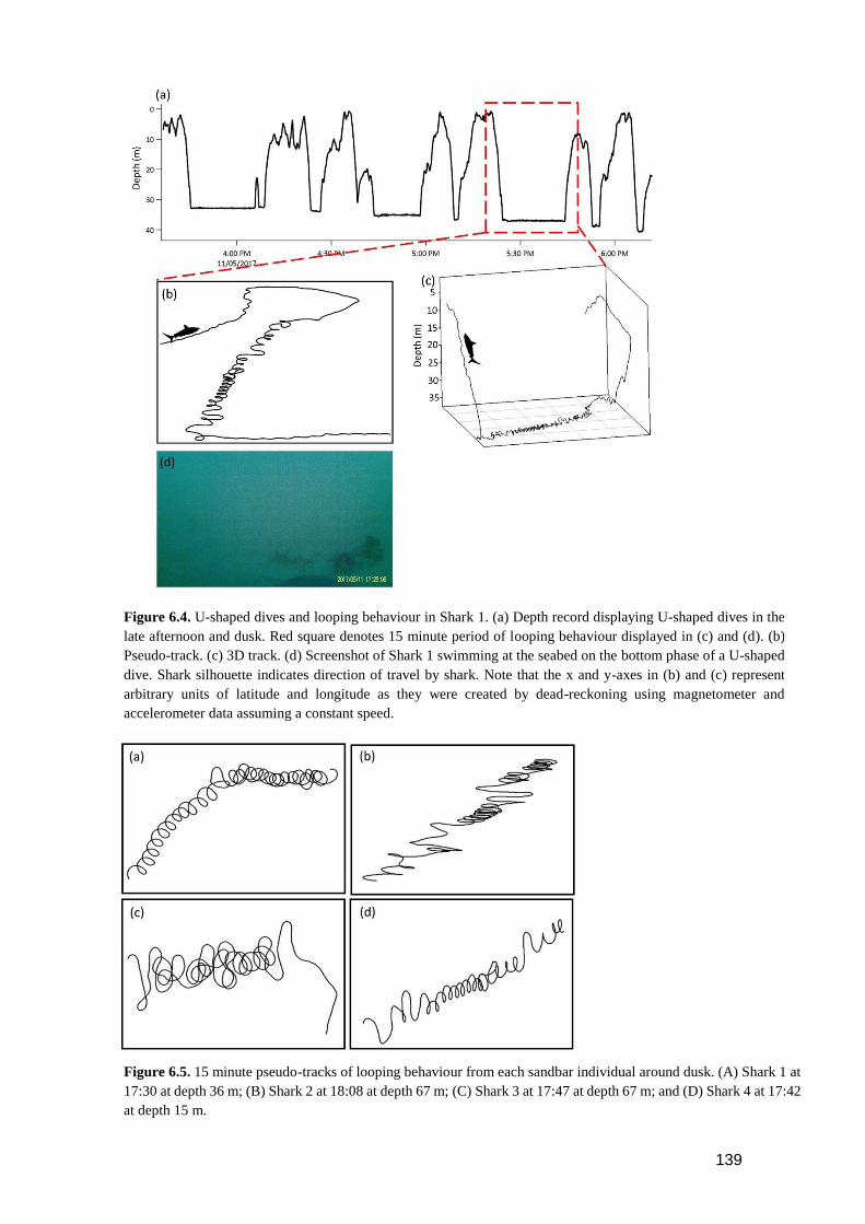
139
Figure 6.4. U-shaped dives and looping behaviour in Shark 1. (a) Depth record displaying U-shaped dives in the
late afternoon and dusk. Red square denotes 15 minute period of looping behaviour displayed in (c) and (d). (b)
Pseudo-track. (c) 3D track. (d) Screenshot of Shark 1 swimming at the seabed on the bottom phase of a U-shaped
dive. Shark silhouette indicates direction of travel by shark. Note that the x and y-axes in (b) and (c) represent
arbitrary units of latitude and longitude as they were created by dead-reckoning using magnetometer and
accelerometer data assuming a constant speed.
Figure 6.5. 15 minute pseudo-tracks of looping behaviour from each sandbar individual around dusk. (A) Shark 1 at
17:30 at depth 36 m; (B) Shark 2 at 18:08 at depth 67 m; (C) Shark 3 at 17:47 at depth 67 m; and (D) Shark 4 at 17:42
at depth 15 m.

140
Figure 6.6. Five minute 3D tracks and pseudo-tracks of turning behaviour throughout the ascents and
descents of U-shaped dives and V-shaped dives. X and Y axes represent arbitrary units of latitude (P-lat)
and longitude (P-long) as they were created by dead-reckoning using magnetometer and accelerometer data
assuming a constant speed. The Z axes in the 3D plots represents depth (m).
6.4.3 Video
The six hours of video validated gliding and turning behaviour, and identified seabed habitat at
the bottom of dives. No interactions with prey or conspecifics were observed, and the only other
animals observed were trevally accompanying the shark, and one school of baitfish briefly
swimming through the field of view. For Shark 1, a 24 minute video recorded a U-shaped dive at
dusk. The video confirmed the bottom phase of the dive occurred at the seabed in a sandy habitat
with patchy weed and reef, and validated the circling behaviour (Supplementary Video 2).

141
6.5 Discussion
Our deployment of biologging tags on adult female sandbar sharks revealed oscillatory and
tortuous movement paths. Tagged sharks underwent continual V- and U-shaped dives through the
water column, diving at shallow angles and displaying tortuous circling behaviours throughout
the bottom phase of U-shaped dives.
6.5.1 Tortuous circling behaviour
As travelling in a straight line is the most energetically efficient form of movement, the higher
energetic costs of turning should be offset by other benefits, such as enhanced foraging success
(Wilson et al. 2013). Because turn costs increase linearly with angle, Wilson et al. (2013)
predicted that more acute turns should be strongly motivated, and would have a tendency to be
clustered in time and space. The tortuous circling behaviour observed in all sandbar sharks
supported these predictions, occurring on the seabed throughout the bottom phase of U-shaped
dives, and predominately occurring around dusk. Possible explanations for this behaviour include
intra-specific interactions, the presence of favourable oceanographic conditions, or foraging
behaviour. Given that no conspecifics were observed in any of the recorded video, and circling
behaviour was observed in both well-mixed offshore and protected inshore environments, it is
unlikely that intra-specific interactions or oceanographic conditions are acting as the primary
drivers of the recorded patterns. The most likely explanation for such behaviour is that it aids in
foraging in this species.
Tortuous movement paths across a range of both aquatic and terrestrial taxa have been used as a
proxy to identify foraging and may be associated with prey pursuit, or search for prey either upon
encountering a cue or based on past learning experiences (Austin et al. 2006; Wilson et al. 2007;
Byrne and Chamberlain 2012; Papastamatiou et al. 2012; Adachi et al. 2017). Sandbar shark diets
are dominated by demersal fauna, such as bentho-pelagic fishes, cephalopods and crustaceans
(McElroy et al. 2006; Ellis and Musick 2007), and at dusk many nocturnal benthic species emerge
from their diurnal refuges (Helfman 1986). The circling behaviour that sandbar sharks were
recorded to display on the seabed may therefore represent a strategy to increase the chance of
capturing prey at this time. In addition to undertaking circling behaviour on the bottom phase of
U-shaped dives, relatively higher turning angles were recorded on the ascent phase of U-shaped
dives in comparison to V-shaped dives. It is possible that sandbar sharks may also be searching
for prey throughout the ascent phase of U-shaped dives while moving between benthic foraging
patches. On ascent, sharks may be able to search for prey that are backlit and silhouetted against
the surface, and potentially ambush them from below (Martin and Hammerschlag 2012). No
changes in turning angle were observed between dive types during descent, indicating that
individuals may be less motivated to search for prey in this phase.

142
6.5.2 Vertical movements
Previous studies reporting vertical movements of sandbar sharks have found these animals to
reach maximum depths of over 250 m and display diel patterns in movement (Papastamatiou et
al. 2006; Barnes et al. 2016). Barnes et al. (2016) found that sandbar sharks tagged off eastern
Australia exhibited a preference for deeper waters throughout daylight hours. Our fine-scale
movement data showed that sandbar sharks displayed continual patterns of oscillatory vertical
movements in both inshore and offshore habitats that were likely bathymetrically limited,
reaching a maximum depth of 96.6 m. Shallow dive angles occurred throughout the tracks, with
relatively symmetrical patterns in ascent and descent. Due to the limited duration of tag
attachment, we were not able to explore diel patterns in vertical movement, particularly as patterns
during the day were biased to the shallow inshore waters in which the sharks were tagged. U-
shaped dives, however, occurred in both inshore and offshore habitats, predominately around
dusk. Several other species of elasmobranch have been found to display diel patterns in foraging-
related behaviours, with crepuscular periods commonly being associated with enhanced activity
rates (Gleiss et al. 2013; Papastamatiou et al. 2015b; Gleiss et al. 2017b; Papastamatiou et al.
2018b). Despite a potential preference for foraging at this time, sandbar sharks may still feed
opportunistically throughout other diel periods, as occurs in grey reef sharks (Carcharhinus
amblyrhynchos) (Papastamatiou et al. 2018b). This may account for occasional U-shaped dives
observed throughout the night in sandbar shark depth traces (Figure 6.3). However, we again
highlight the limited duration of tag attachment in our study and longer tag deployments are
required to determine if these patterns occur on a diel cycle.
6.5.3 Species comparisons
Repetitive oscillatory movements through the water column are a common feature of the tracks
of nearly all epipelagic fishes for which fine-scale depth traces have been recorded (Carey et al.
1990; Klimley et al. 2002; Schaefer et al. 2009). Recent studies using biologging tags on tiger
sharks (Galeocerdo cuvier) and oceanic whitetip sharks (Carcharhinus longimanus) suggested
that these dives likely function as a means of searching for prey (Nakamura et al. 2011;
Papastamatiou et al. 2018a). However, if sandbar sharks are predominately searching for prey on
the seabed, continual hunting forays through the water column are unlikely to be the primary
motivator of these movements. Alternatively, these animals may be indirectly searching for
benthic prey by oscillating through vertically stratified layers for olfactory cues in between
patches (Carey et al. 1990; Klimley et al. 2002). In addition, data from tri-axial sensors suggest
that they are doing so in an energetically efficient manner. Shallow dive angles and gliding
behaviour appear to be common feature of the vertical movements of all large epipelagic fishes
for which detailed data records are available (Furukawa et al. 2011; Gleiss et al. 2011b; Gleiss et
al. 2011c; Meekan et al. 2015; Papastamatiou et al. 2018a). Given the need to oscillate through

143
the water column to search for cues, shallow dive angles and intermittent gliding behaviour have
been calculated to minimize the cost of transport, culminating in patterns of cost-efficient foraging
(Gleiss et al. 2011b; Papastamatiou et al. 2018a). Sandbar sharks descended at very shallow dive
angles (mean 11.4 ± 2.2° and -11.5 ± 3.5° for ascent and descent respectively), with uninterrupted
glides of up to 210 seconds in duration. These angles are comparable with mean dive angles for
both tiger sharks and whale sharks (Rhincodon typus). Mean ascent and descent angles for tiger
sharks were recorded at 9.4° and -11° respectively (see Chapter 5), and for whale sharks mean
descent angles of 12-13° were documented, with highly variable ascent angles varying 10-25°
depending on dive type (Gleiss et al. 2011b). The shallower dive angles were estimated to
minimize the cost of horizontal travel for whale sharks, and may have been near the minimum
angle required for gliding to be possible. However, in contrast to sandbar sharks, whale sharks
would continuously glide on a majority of descents. A number of factors may be responsible for
these inter-specific differences in gliding behaviour, including body composition (i.e. ratio lipids
to lean tissue) (Gleiss et al. 2017a), morphometrics influencing lift and drag, and the increased
drag incurred by smaller sharks carrying relatively large biologging tags.
6.5.4 Limitations and future considerations
Despite our limited sample size and tag attachment durations, consistent patterns emerged among
tagged individuals. Populations of sandbar sharks at Ningaloo mostly consist of adult females
(Braccini and Taylor 2016; Braccini et al. 2017), therefore tagging in other locations will likely
be required to obtain a more representative sample of both sexes and all size classes. Durations
of attachment (>24 hours) in our study were limited by our need to recover biologging tags to
download the data. Offshore swimming behaviour of the tagged individuals meant that the
distances involved in tag recovery following 24 hours of attachment were at the limit of our VHF
radio range and offshore boat license in two cases (25-30 km). Longer durations of tag attachment
will provide a greater understanding of diel cycles of movement in this species, and an increased
capacity to record and store video will aid in revealing more about the drivers of movements,
particularly in relation to foraging behaviours. We also acknowledge that the recovery rate of
sharks from capture processes can be difficult to define, and that we may not be recording natural
behaviours in our current study. Although continuous glides of up to 210 seconds were recorded
by sandbar sharks, sparse tailbeats frequently interrupted gliding descents. The possibility that
drag due to the tag (Whitney et al. 2019) may be playing a role in inhibiting natural gliding
behaviours in this and other studies that use relatively large biologging devices requires future
investigation. Lastly, accurate speed measurements and GPS anchor points would considerably
enhance dead-reckoning analyses, allowing further insight into fine-scale locational and habitat
preferences (Walker et al. 2015).
144
6.5.5 Conclusions
Evaluating the results of our study in the context of broad scale ecological knowledge for the
species provided new ecological insights into the fine spatial and temporal scale movement
behaviours of the sandbar shark. Collectively, patterns recorded by biologging tags on sandbar
sharks suggested energetically efficient oscillatory swimming behaviours whilst moving between
benthic hunting patches, consistent with biologging studies emphasizing the role of cost-efficient
foraging. Larger sample sizes with extended tag recording durations will enable greater ecological
insight into these behaviours.
6.6 Acknowledgements
We thank Murdoch University and Coral Bay Research Station for accommodation and vessel
use while conducting fieldwork. This work would not have been possible without the generous
support of numerous field volunteers, particularly: Karissa Lear, Frazer McGregor, Abraham
Sianipar, Adam Jolly, Evan Byrnes, Garry Teesdale and Michael Tropiano. Nikolai Liebsch
provided invaluable assistance with tag functioning. We are grateful to Lauren Peel and two
reviewers, whose comments greatly improved this manuscript.

145
6.7 Supporting Information
Supplementary Video 2: https://vimeo.com/303182717
Password: shark
Figure S 6-1. Mean and sd of tailbeat cycles (inverse of tailbeat frequency) during descent for individual
sandbar sharks over 15 minute windows. (a) Shark 1; (b) Shark 2; (c) Shark 3; and (d) Shark 4.
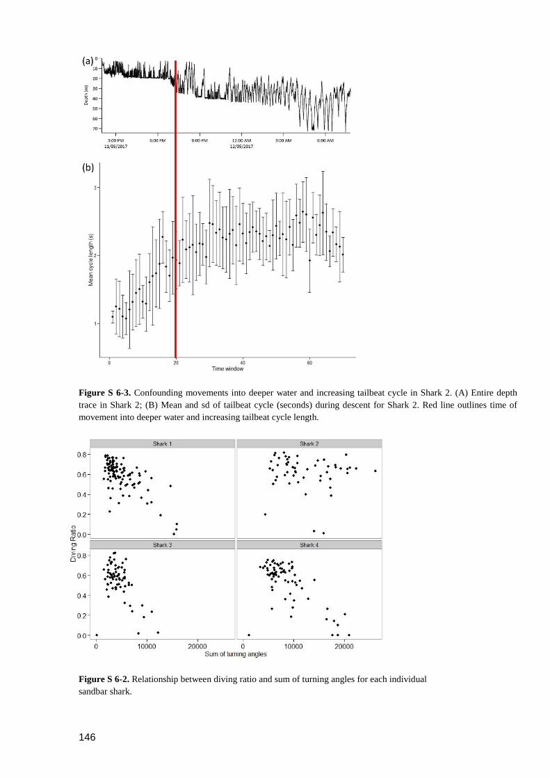
146
Figure S 6-3. Confounding movements into deeper water and increasing tailbeat cycle in Shark 2. (A) Entire depth
trace in Shark 2; (B) Mean and sd of tailbeat cycle (seconds) during descent for Shark 2. Red line outlines time of
movement into deeper water and increasing tailbeat cycle length.
Figure S 6-2. Relationship between diving ratio and sum of turning angles for each individual
sandbar shark.

147
Table S 6.1. Linear model comparisons using Akaike’s Information Criterion (AIC), R2, and p-values.
ΔAIC displays deviance in AIC scores from null model. Diving ratio (DR) is modelled as a function of
turning. Turning has been subset for each vertical phase of movement (level swimming, ascending and
descending), and standardised by the time spent in that phase within a sampling window.
Shark ID Model Slope AIC ΔAIC R2 p
Shark 1 DR ~ level turning
DR ~ 1
-0.02 -176
-138
38 0.32 <0.001
Shark 2 DR ~ level turning
DR ~ 1
-0.001 -83
-84
-1 0.01 0.5
Shark 3 DR ~ level turning
DR ~ 1
-0.03 -98
-64
34 0.40 <0.001
Shark 4 DR ~ level turning
DR ~ 1
-0.02 -81
-47
34 0.42 <0.001
Shark ID Model Slope AIC ΔAIC R2 p
Shark 1 DR ~ ascent turning
DR ~ 1
-0.02 -153
-138
15 0.15 <0.001
Shark 2 DR ~ ascent turning
DR ~ 1
-0.002 -84
-84
0 0.04 0.003
Shark 3 DR ~ ascent turning
DR ~ 1
-0.03 -71
-64
7 0.12 0.15
Shark 4 DR ~ ascent turning
DR ~ 1
-0.02 -59
-47
12 0.19 <0.001
Shark ID Model Slope AIC ΔAIC R2 p
Shark 1 DR ~ descent turning
DR ~ 1
-0.007 -141
-138
3 0.05 0.03
Shark 2 DR ~ descent turning
DR ~ 1
-0.001 -83
-81
-1 0.009 0.52
Shark 3 DR ~ descent turning
DR ~ 1
-0.02 -67
-64
3 0.07 0.02
Shark 4 DR ~ descent turning
DR ~ 1
-0.009 -48
-47
1 0.05 0.08

148
Chapter 7 General Discussion
Advances in the affordability and sophistication of electronic tags now allow researchers to
routinely document the vertical movements of large, epipelagic fishes (>30 kg adult size). Despite
the increasing research focus, there has been no standardised approach to classify these
behaviours and investigate their physical and biological drivers. This thesis aimed to review the
existing knowledge of the vertical movements of large, epipelagic fishes, and improve our
understanding of the underlying factors structuring these behaviours through several case studies.
Through a synthesis of the existing knowledge of vertical movements, I was able to provide a
framework to investigate the drivers of these patterns in future studies (Chapter 2). I then used
this framework to explore some of the key drivers highlighted in the synthesis, using advanced
tagging technologies and new analytical techniques at seasonal (Chapter 3) and fine scales
(Chapters 4, 5 and 6, Figure 7.1). There were two common themes through all of my chapters.
Firstly, cost-efficient foraging appears to play a significant role in the vertical movements of large,
epipelagic fishes. Secondly, our overall understanding of these patterns is limited by tagging
technologies, and as a result, I highlight the important trade-offs in data resolution and
deployment duration that must be considered before commencing studies of this kind. I argue that
patterns of vertical movement result from the need for ram ventilating animals to move
continuously in a 3D environment while simultaneously optimizing prey encounter, energy
expenditure and remaining within physical limits imposed by the environment on their
physiology, and that an understanding of such patterns is beneficial to conservation efforts in the
context of a warming ocean.
Figure 7.1. Schematic of the timeline of different processes that may influence patterns of vertical
movement in large, epipelagic fishes. Dashed squares denote the time periods for which biologging tags
and recovered satellite tags will be most effective.

149
7.1 Seasonal scales of vertical movement
Due to limited band width of satellite communications, data from satellite-linked tags are typically
transmitted in a summarized form (histograms in pre-defined bins), preventing the detailed
reconstruction of relationships between depth and temperature (Chapter 2). However, the rare
recovery of these tags and subsequent download of detailed data sets archived within the tag
provides us with the opportunity to explore these relationships in detail at seasonal time scales
(Chapter 2). Depth and temperature archives from 16 recovered satellite tags enabled me to
investigate how seasonal changes in the thermal environment influenced the vertical movement
patterns of a large, epipelagic, ectothermic shark (Chapter 3). As the water column warmed and
stratified in summer months, oceanic whitetip sharks in the North Atlantic Ocean were observed
to reduce the proportion of time spent in the upper 50 m of the water column and to increase the
amplitude of their oscillatory movements. These patterns of vertical movement allowed
individuals to maintain a relatively stable mean daily temperature year-round, despite much larger
annual changes in mean sea surface temperatures. Such behaviours likely represent behavioural
thermoregulation, a strategy to maintain a favourable body temperature (Chapter 3).
Neill et al. (1979) proposed that a fish that successfully thermoregulates will move through its
habitat in a way that allows it to maximize time spent within a preferred temperature range where
physiological processes are optimised. However, there may be discrepancies between this range
and the distribution of prey, and for this reason, these animals may need to perform physiological
and/or behavioural thermoregulation to avoid reaching critical temperature limits when foraging
(Chapter 2). Thermoregulation has typically been described by tagging studies as a process
whereby large, epipelagic fishes utilize surface waters to warm up between periods of foraging in
cooler and deeper habitats (positive thermotaxis, Chapter 2) (Carey et al. 1990; Klimley et al.
2002; Abecassis et al. 2012; Thums et al. 2013; Nakamura et al. 2015a). However, at a time where
the consequences of a warming climate are a major concern for marine ecosystems, and given the
asymmetric shape of the thermal performance curve (Martin and Huey 2008), it is somewhat
surprising that the reverse pattern has not been described to a greater extent.
Ectothermic fishes in tropical epipelagic systems, where waters are warm and prey sparsely
distributed, pose an interesting case when considering thermal tolerance. Large ectothermic fish
in these environments will have high metabolic rates, and in order to survive, they need to be cost-
efficient foragers and maintain their body temperatures within an optimal range. Oceanic whitetip
sharks were able to do this by shifting their vertical behaviours and distribution on a seasonal
scale (Chapter 3). In this case, temperature appeared to be a physiological driver of vertical
movements (Chapter 2), setting an upper limit to vertical distributions. An interesting finding was
that there was individual variability in the vertical movement behaviours used to thermoregulate.
Shark size and migratory phase did not appear to be responsible for these patterns. Beyond this,
150
the data gathered by the tag did not allow me to determine the processes driving these differences.
In addition, oscillatory movements continued in winter months when the water-column was well-
mixed, indicating that an ecological driver (Chapter 2) may be influencing how these animals
moved within their physiological limits. Insight into these patterns of vertical movement on a
seasonal scale was made possible through the long-term deployment and retrieval of archival
satellite tags, however, a biologging approach may enable the ecological driver(s) and individual
differences to be more clearly determined.
7.2 Biologging and fine-scale patterns of vertical
movement
Recent advances in biologging technologies have fundamentally enhanced our understanding of
the fine-scale (seconds to days, m to km) movements of marine megafauna (Bograd et al. 2010;
Goldbogen et al. 2013a). The additional sensors and high resolution of data recorded by these tags
have documented detail well beyond that of the traditional depth and temperature logs produced
by conventional tagging technologies. At fine-scales, oscillatory movement patterns are a
common feature of the tracks of nearly all epipelagic fishes for which high-resolution depth traces
are available (Chapter 2). By using advanced biologging tags, I was able to investigate the role of
cost-efficient foraging in driving these patterns in tiger sharks and sandbar sharks. Data from these
tags revealed how vertical oscillations were linked to energetics, kinematics, prey interactions,
and fine-scale habitat use.
Initially, I demonstrated the utility of these tags to document complex movement behaviours in
tiger sharks that would otherwise be invisible within time-depth records (Chapter 4). I found that
oscillatory movements occurred not only during directional travel, but continued throughout the
tortuous movements that are likely to be associated with foraging behaviour. This suggests that
the vertical movements of tiger sharks were not primarily driven by prey search alone as
hypothesized in previous studies (Chapter 4; Heithaus et al. 2002b; Nakamura et al. 2011). To
investigate if oscillatory movements were also a strategy for conservation of energy, I modelled
the cost of transport of varying movement geometries using overall dynamic body acceleration
(ODBA) as a proxy for energy expenditure (Chapter 5; Gleiss et al. 2011b). I found that tiger
sharks could reduce their cost of horizontal transport relative to level swimming by swimming at
shallow dive angles, and this supported my hypothesis that conservation of energy was a primary
factor in the oscillatory movement patterns I observed (Chapter 5). Energy savings were likely
optimized in very shallow environments (<3 m), where tiger sharks were able to continuously
search for prey at the surface and seabed while exploiting the most cost-efficient dive angles. In
deeper environments, however, tiger sharks encountered added energy costs from transiting a
longer distance through the water column between the surface and the seabed, and to compensate,
they displayed steeper angles that reduced the cost of vertical transport (Chapter 5).

151
Tiger sharks are a well-studied and charismatic species, and a number of previous studies have
explored their fine-scale vertical movements (E.g. Holland et al. 1999; Heithaus et al. 2002b;
Nakamura et al. 2011; Afonso and Hazin 2015). In contrast, sandbar sharks are less charismatic,
and their commercial importance has led previous studies to focus on their broad-scale (10-1000
km) horizontal movement patterns, with only brief descriptions of vertical movements
(Papastamatiou et al. 2006; Barnes et al. 2016). By using a biologging approach, I was able
examine these vertical movements at a fine-scale for the first time, and to reveal energetically
efficient oscillatory diving behaviours in sandbar sharks (Chapter 6). As with the tiger sharks, the
dive angles used by this species were very shallow, and gliding behaviour was observed in all
four tagged individuals. In addition, the fine-scale depth record exposed two different vertical
movement patterns in this species; U-shaped dives and V-shaped dives. U-shape dives occurred
most frequently around dusk and dead-reckoning using accelerometer and magnetometer data
recorded highly tortuous, circling tracks on their bottom phase. Given the largely benthic diet of
the sandbar shark, I believe this vertical movement behavior is a strategy for hunting emergent
benthic prey (Chapter 6).
The biologging approach described above revealed disparities and similarities between the
vertical paths of tiger and sandbar sharks. Tiger sharks exhibited an affinity for shallower waters
where they could reduce the cost of transport while searching the surface and seabed, and
displayed no relationship between oscillatory and tortuous horizontal movements (Chapter 4, 5).
Sandbar sharks displayed V- and U-shaped dives in both inshore and offshore habitats, with the
tortuosity of movements increasing with bottom time (Chapter 6). I argue that these contrasting
patterns are a function of inter-specific differences in foraging ecology. Tiger sharks are likely
transiting continuously through the water column to search for prey and scavenging opportunities
at the surface and near the seabed (Simpfendorfer et al. 2001), while sandbar sharks are
predominately searching for demersal prey at a level depth along the seabed (McElroy et al. 2006)
before using vertical movements to travel between benthic hunting patches. Despite foraging in a
different manner within distinct regions of the water column, however, both species were found
to display patterns of energetically efficient oscillatory swimming.
The expanding use of biologging tags on sharks and other large epipelagic fishes is revealing
common patterns in the energetics and kinematics of oscillatory movement behaviours of these
animals. For example, shallow dive angles and/or gliding behaviour have now been recorded for
oceanic whitetip (Papastamatiou et al. 2018a), whale (Rhincodon typus; Gleiss et al. 2011a), white
(Carcharodon carcharias; Gleiss et al. 2011c), tiger (Chapter 5) and sandbar (Chapter 6) sharks.
It has also been recorded in dolphinfish (Coryphaena hippurus) and Pacific bluefin tuna (Thunnus
orientalis) (Furukawa et al. 2011; Noda et al. 2016). The diversity of habitats, distribution and
feeding ecologies among these species suggests that shallow, energetically efficient dive angles
and gliding behaviour may be commonplace in large epipelagic fishes, and as a result, cost-

152
efficient foraging a primary driver of vertical movements at fine-scales. The approaches used in
this thesis are likely to be of use for studying the movements of other animals that move in three-
dimensions, notably flying animals.
7.3 Temporal scale and vertical movements
All case studies in this thesis utilized data from tags that had been physically recovered,
highlighting the applicability of these data sets to investigations of the patterns and drivers of
vertical movements in large epipelagic fishes. It remains significant to future studies of vertical
movements to emphasise the importance of determining the temporal scale of interest before
forming specific hypotheses and selecting a tagging technique, given the short deployment
periods of biologging tags in contrast to the durations that are feasible for satellite tags and the
recovery period associated with most tagging procedures.
Biologging tags enabled fine-scale patterns to be recorded that could then be compared to habitat
use, diel phase and environmental temperature. In the case of tiger and sandbar sharks at Ningaloo
Reef, no changes in environmental temperature were observed in this well-mixed, shelf
environment, precluding examination of the role of this driver on the vertical movement patterns
of these species. Absence of a temperature gradient was beneficial as it eliminated the possibility
of this variable playing a synergistic role with other drivers, however, well-mixed water columns
are a feature mostly limited to shallow coastal shelves. Because they encompassed a much longer
period of deployment (up to a year) where animals moved across coastal and oceanic habitats,
recovered satellite tag data from oceanic whitetip sharks recorded seasonal changes in the water
column and allowed me to investigate the role of environmental temperature on vertical
movements. The disparity between the environmental temperature datasets collected in these
studies highlight how these two tagging methods can currently be used to separately address
drivers at different scales (Figure 7.1). Delayed tag activation, onboard processing and cameras
triggered by predetermined movement thresholds (e.g. Naito et al. 2017) may help in extending
biologging tag recording duration in the future. Until the deployment duration of biologging tags
can be extended to that currently available from satellite tags, however, a comprehensive
understanding of the collective patterns and drivers of vertical movements of epipelagic fishes
will require these two discrete tag types.
7.4 Limitations and future directions
The choice of tag type for a study is currently a tradeoff between deployment duration, data
resolution, tag cost and sensor capabilities. In an ideal world, biologging tags with a wide range
of high-resolution sensors would be deployed on a representative cross-section of a population of
large epipelagic fishes for seasonal to annual scales, enabling thorough investigation of
153
energetics, kinematics, foraging, and physiological limits at all temporal scales of movement.
Given current battery and storage limitations, high costs, the need to recover these tags to
download archived data, and the likely influence of physical variables that require sensors (e.g.
oxygen concentration) not typically available in tags, however, this remains a goal for future tag
development.
Alongside advancing the battery life and storage capabilities of biologging tags, additional
sensors are being developed and trialed, and will soon enable more hypotheses driven approach
to vertical movement studies. For example, dissolved oxygen sensors in satellite tags (Coffey and
Holland 2015) will allow us to test the influence of this physical factor as a physiological driver
on the vertical movement patterns of epipelagic fishes over seasonal time scales. For oceanic
whitetip sharks, these tags would allow us to determine if dissolved oxygen concentration is acting
synergistically with environmental temperature to produce the observed seasonal scale patterns
in Chapter 3, as was found to be the case in salmon sharks (Lamna ditropis) (Coffey et al. 2017).
These will also provide insight into the physiology of epipelagic fishes and their capacity to
tolerate low oxygen concentrations. Sonar tags are also being trialed, and will allow focal species
to map the prey field that they encounter during a dive (Lawson et al. 2015). These tags would
allow testing of hypotheses attributing oscillatory diving to prey search (see Chapter 2), and
reduce a reliance on video for this task, which is both battery hungry and requires large data
storage capacity.
There is currently no solution to extend the sampling duration of biologging tags, largely because
of the need to physically recover the devices. Where accelerometers have been incorporated into
acoustic tags to enable longer-term studies of activity and metabolic rate (Papastamatiou et al.
2015b; Barnett et al. 2016), transmissions are typically summarized into lower resolution time
bins, and patterns with vertical habitat use are masked (Whitney et al. 2019). Until we are able to
provide a means to both extend the deployment duration of high-resolution tags and ensure
retrieval of the full, high-resolution data sets, recovered archival tags provide the most practical
means to gain insights into the drivers of epipelagic fish vertical movements on larger temporal
scales.
Whereas advances towards extending the temporal scales over which the vertical movement
patterns of an individual can be monitored are ongoing, it is also interesting to consider how such
patterns might change throughout the lifetime of the individual. Acoustic tags currently provide
the longest view (multiple years) into the movement patterns of epipelagic fishes and are an
affordable means to obtain population-scale estimates of movement behaviour, however,
sampling periods are restricted to when tagged individuals enter the boundary of a receiver array.
Satellite tags overcome the spatial restrictions imposed by acoustic tags and receivers, but are
rarely attached to individuals for over one year (Chapter 2). In cases where tag attachment exceeds

154
an annual cycle, collected data is still of a relatively low resolution, preventing a detailed
assessment of how drivers vary in their impact on ontogenetic scales (Figure 1). For these reasons,
previous studies investigating how vertical movements change with increasing body size have
been limited to comparisons among individuals of different sizes (E.g. Afonso and Hazin 2015;
Williams et al. 2017b), rather than observation of changes as an individual grows. Although not
ideal, these studies have enabled insights into how ontogenetic differences in foraging behaviour
and/or physiology may drive changes in vertical movements, highlighting the benefits of tagging
representative cross-sections of a population (Chapter 2), and providing added motivation for the
continued development and improvement of biologging techniques.
The challenges of assessing patterns of vertical movement in large epipelagic fishes are not only
restricted to technology. The logistics, ethics and often opportunistic nature of field sampling,
generate difficulties in obtaining the large and representative sample sizes of study species that
are necessary to understand movement drivers for a population as a whole. Tag deployments are
also ethically constrained to individuals of a minimum size, precluding attachment to juveniles
until this size is attained. The expense of field operations, coupled with the need to retrieve tags
to download collected data means that tag deployments are often limited to coastal areas and
restricted to a non-migrating portion of the population. As many species of shark also tend to
segregate by sex and size (Sims 2005; Speed et al. 2010), sampling will often be biased by the
regional composition of the population. In this thesis, adult females comprised the majority of the
tagging cohort (93%), likely reflecting the composition of the respective study region (Chapters
3, 4 & 6). The one male oceanic whitetip shark tagged in Chapter 3 was the only individual of
this species to not show a thermoregulatory strategy. Further sampling of males is therefore
required to explore the possibility that male oceanic whitetips have a wider thermal range
compared to females. The continuing advance of tagging technologies will enable us to address
these issues in future studies. Miniaturization and extended recording durations will enhance our
capacity to tag a more representative portion of the population, as well as to investigate vertical
movements throughout both resident and migratory phases of a species.
7.5 Implications
The combination of high commercial importance and k-selected life history traits in many large,
epipelagic fishes (Chapter 2) means that the odds of continued survival are already stacked against
this group of animals. Given the importance of remaining within an optimal thermal range, global
climate change could further lower these odds by expanding regions of the water column that are
unsuitable for these taxa to inhabit. Epipelagic species in a warming ocean are more likely to
encounter upper thermal limits in surface waters, and could use vertical behaviours to avoid
prolonged exposure to these temperatures as a result (Chapter 3). This behavioural shift would
have repercussions for available foraging time and space, particularly as there may be mismatches
155
with how prey distributions respond to warming temperatures (Edwards and Richardson 2004;
Hazen et al. 2013). Fishes with higher energy demands, such as tuna and billfishes (Wegner et al.
2010), are hypothesised to pay a high energetic price to find prey, maximize energy surplus per
unit time, and together, lead a life of high energy turnover (Papastamatiou et al. 2018a). Warming
waters may then increase the susceptibility of these fishes to overheating (Gilman et al. 2016),
resulting in the generation of higher metabolic rates that require supplementary energy intake,
and amplifying the consequences of trophic mismatch. Conversely, large epipelagic fishes with
lower metabolic rates, such as ectothermic sharks (Dowd et al. 2006), likely utilize cost-efficient
strategies that enable them to expend less energy to find prey (Chapter 5), lowering the rate of
energy turnover and surplus in these species (Papastamatiou et al. 2018a). These animals,
however, have a lower probability of food acquisition per unit time and are more liable to
starvation and breeding failure (Wilson et al. 2018). A reduction in available foraging time and
space, coupled with prey mismatch, could then further thin this energetic knife-edge on which
they currently live, increasing the probability of mortality through exhausted energy reserves in
these taxa (Wilson et al. 2018).
The ability of large epipelagic fishes to adapt to these environmental impacts is questionable given
the accelerated rates of climate change (Intergovernmental Panel on Climate Change 2013), in
addition to the synergistic effect of other anthropogenic threats. Conservation and management
strategies therefore need to be adaptive, and focus on ensuring that populations remain resilient
to give them the best chances of survival (Fuentes et al. 2016). Adaptive management takes
advantage of new information that will improve management outcomes. Examples of such
information that would improve management strategies were found in this thesis.
Firstly, given that different fishing gears target different depths, an understanding of how
temperature influences vertical movement behaviour of oceanic whitetip sharks (Chapter 3) will
enable adaptive management by both target and non-target fisheries. The avoidance of surface
waters by this species in summer months will reduce the susceptibility of individuals to surface-
set fishing gears, but may increase their vulnerability to deeper-set longlines (Chapter 3). Fisheries
management could take advantage of this information by introducing temporal changes in
management strategies and fishing practices. Secondly, at finer-scales, biologging tags enabled
better understanding of habitat use in two species of coastal shark. Tiger and sandbar sharks
display patterns of residency in coastal and well-mixed regions (Ferreira et al. 2015; Braccini et
al. 2017), and warming temperatures may instead elicit shifts to higher latitudes. Understanding
the patterns of fine-scale movement and habitat use will enable us to foresee the viability of these
range shifts. Shallow habitats, for example, were found to be an important area for tiger sharks to
reduce energy expenditure while hunting (Chapter 5). Identifying these key foraging areas will
assist in optimizing strategies for spatial protection such as marine protected areas (MPAs), the
efficacy of which will be maximized by allowing them to be adaptive and compensate for future

156
range shifts.
7.6 Concluding remarks
My thesis demonstrated how tagging datasets can enable us to improve our understanding of the
patterns and drivers of vertical movements in large, epipelagic fishes. I examined and
acknowledged the trade-offs between biologging and satellite tagging technologies and their
ability to target specific temporal resolutions of vertical movement. Through both my methods
and results, I provide a framework for future studies to continue to explore and understand vertical
movements in these animals using both tag types. I argue that patterns of vertical movement result
from the need for gill-breathing animals to move continuously in a 3D environment while
optimising food encounter, energy expenditure and remaining within limits imposed by the
physical environment on their physiology. The expanding use of biologging tags on large fishes
will continue to uncover cryptic behaviours, and provide revelations about movements in
environments where they would otherwise be very difficult to observe. Representative sampling
of populations and extended deployment durations of high resolution biologging tags will enable
us to continue improving our understanding of vertical movements in these charismatic taxa and
in so doing, generate the knowledge base essential for determining the impacts of a warming
ocean on these species.

157
Bibliography
Abascal F, Quintans M, Ramos-Cartelle A, Mejuto J (2011) Movements and environmental preferences
of the shortfin mako, Isurus oxyrinchus, in the southeastern Pacific Ocean. Marine Biology
158:1175-1184
Abascal FJ, Mejuto J, Quintans M, Ramos-Cartelle A (2010) Horizontal and vertical movements of
swordfish in the Southeast Pacific. ICES Journal of Marine Science: Journal du Conseil 67:466-
474
Abecassis M, Dewar H, Hawn D, Polovina J (2012) Modeling swordfish daytime vertical habitat in the
North Pacific Ocean from pop-up archival tags. Marine Ecology Progress Series 452:219-236
Acuña-Marrero D, Smith ANH, Hammerschlag N, Hearn A, Anderson MJ, Calich H, Pawley MDM,
Fischer C, Salinas-de-León P (2017) Residency and movement patterns of an apex predatory
shark (Galeocerdo cuvier) at the Galapagos Marine Reserve. PLOS ONE 12:e0183669
Adachi T, Costa DP, Robinson PW, Peterson SH, Yamamichi M, Naito Y, Takahashi A (2017) Searching
for prey in a three-dimensional environment: hierarchical movements enhance foraging success
in northern elephant seals. Functional Ecology 31:361-369
Adachi T, Maresh JL, Robinson PW, Peterson SH, Costa DP, Naito Y, Watanabe YY, Takahashi A
(2014) The foraging benefits of being fat in a highly migratory marine mammal. Proceedings of
the Royal Society B: Biological Sciences 281
Afonso AS, Hazin FH (2014) Post-release survival and behavior and exposure to fisheries in juvenile
tiger sharks, Galeocerdo cuvier, from the South Atlantic. Journal of Experimental Marine
Biology and Ecology 454:55-62
Afonso AS, Hazin FH (2015) Vertical movement patterns and ontogenetic niche expansion in the tiger
shark, Galeocerdo cuvier. PLoS ONE 10:e116720
Aguilar Soto N, Johnson Mark P, Madsen Peter T, Díaz F, Domínguez I, Brito A, Tyack P (2008)
Cheetahs of the deep sea: deep foraging sprints in short-finned pilot whales off Tenerife (Canary
Islands). Journal of Animal Ecology 77:936-947
Andrews KS, Williams GD, Farrer D, Tolimieri N, Harvey CJ, Bargmann G, Levin PS (2009) Diel
activity patterns of sixgill sharks, Hexanchus griseus: the ups and downs of an apex predator.
Animal Behaviour 78:525-536
Andrzejaczek S, Gleiss AC, Jordan LKB, Pattiaratchi CB, Howey LA, Brooks EJ, Meekan MG (2018)
Temperature and the vertical movements of oceanic whitetip sharks, Carcharhinus longimanus.
Scientific Reports 8:8351
Angilletta MJ, Niewiarowski PH, Navas CA (2002) The evolution of thermal physiology in ectotherms.
Journal of Thermal Biology 27:249-268
Austin D, Bowen WD, McMillan JI, Iverson SJ (2006) Linking movement, diving, and habitat to foraging
success in a large marine predator. Ecology 87:3095-3108
Bancroft K (2003) A standardised classification scheme for the mapping of shallow-water marine habitats
in Western Australia. Marine Conservation Branch, Department of Conservation and Land
Management, Report MCB-05/2003, Fremantle, Western Australia
Barnes CJ, Butcher PA, Macbeth WG, Mandelman JW, Smith SDA, Peddemors VM (2016) Movements
and mortality of two commercially exploited carcharhinid sharks following longline capture and
release off eastern Australia. Endangered Species Research 30:193-208
Barnett A, Payne NL, Semmens JM, Fitzpatrick R (2016) Ecotourism increases the field metabolic rate of
whitetip reef sharks. Biological Conservation 199:132-136
Barnett A, Abrantes KG, Stevens JD, Bruce BD, Semmens JM (2010) Fine-scale movements of the
broadnose sevengill shark and its main prey, the gummy shark. PLoS ONE 5:e15464
Baum JK, Myers RA (2004) Shifting baselines and the decline of pelagic sharks in the Gulf of Mexico.
Ecology Letters 7:135-145
Baum JK, Worm B (2009) Cascading top-down effects of changing oceanic predator abundances. Journal
of Animal Ecology 78:699-714
Bernal D, Carlson JK, Goldman KJ, Lowe CG (2012) Energetics, metabolism, and endothermy in sharks
and rays. In: Carrier J, Musick JA, Heithaus Michael R (eds) Biology of sharks and their
relatives. CRC Press, Boca Raton,
Bessudo S, Soler GA, Klimley PA, Ketchum J, Arauz R, Hearn A, Guzmán A, Calmettes B (2011)
Vertical and horizontal movements of the scalloped hammerhead shark (Sphyrna lewini) around
Malpelo and Cocos Islands (Tropical Eastern Pacific) using satellite telemetry. Boletín de
Investigaciones Marinas y Costeras-INVEMAR 40:91-106
Bestley S, Gunn JS, Hindell MA (2009) Plasticity in vertical behaviour of migrating juvenile southern
bluefin tuna (Thunnus maccoyii) in relation to oceanography of the south Indian Ocean.
Fisheries Oceanography 18:237-254

158
Biais G, Coupeau Y, Séret B, Calmettes B, Lopez R, Hetherington S, Righton D (2017) Return migration
patterns of porbeagle shark (Lamna nasus) in the Northeast Atlantic: implications for stock range
and structure. ICES Journal of Marine Science 74:1268-1276
Bigelow KA, Maunder MN (2007) Does habitat or depth influence catch rates of pelagic species?
Canadian Journal of Fisheries and Aquatic Sciences 64:1581-1594
Bird CS, Veríssimo A, Magozzi S, Abrantes KG, Aguilar A, Al-Reasi H, Barnett A, Bethea DM, Biais G,
Borrell A, Bouchoucha M, Boyle M, Brooks EJ, Brunnschweiler J, Bustamante P, Carlisle A,
Catarino D, Caut S, Cherel Y, Chouvelon T, Churchill D, Ciancio J, Claes J, Colaço A, Courtney
DL, Cresson P, Daly R, de Necker L, Endo T, Figueiredo I, Frisch AJ, Hansen JH, Heithaus M,
Hussey NE, Iitembu J, Juanes F, Kinney MJ, Kiszka JJ, Klarian SA, Kopp D, Leaf R, Li Y,
Lorrain A, Madigan DJ, Maljković A, Malpica-Cruz L, Matich P, Meekan MG, Ménard F,
Menezes GM, Munroe SEM, Newman MC, Papastamatiou YP, Pethybridge H, Plumlee JD,
Polo-Silva C, Quaeck-Davies K, Raoult V, Reum J, Torres-Rojas YE, Shiffman DS, Shipley
ON, Speed CW, Staudinger MD, Teffer AK, Tilley A, Valls M, Vaudo JJ, Wai T-C, Wells RJD,
Wyatt ASJ, Yool A, Trueman CN (2018) A global perspective on the trophic geography of
sharks. Nature Ecology & Evolution 2:299-305
Block B, Booth D, Carey F (1992) Depth and temperature of the blue marlin, Makaira nigricans,
observed by acoustic telemetry. Marine Biology 114:175-183
Block B, Keen J, Castillo B, Dewar H, Freund E, Marcinek D, Brill R, Farwell C (1997) Environmental
preferences of yellowfin tuna (Thunnus albacares) at the northern extent of its range. Marine
Biology 130:119-132
Block BA, Dewar H, Blackwell SB, Williams TD, Prince ED, Farwell CJ, Boustany A, Teo SL, Seitz A,
Walli A (2001) Migratory movements, depth preferences, and thermal biology of Atlantic
bluefin tuna. Science 293:1310-1314
Block BA, Jonsen ID, Jorgensen SJ, Winship AJ, Shaffer SA, Bograd SJ, Hazen EL, Foley DG, Breed
GA, Harrison AL, Ganong JE, Swithenbank A, Castleton M, Dewar H, Mate BR, Shillinger GL,
Schaefer KM, Benson SR, Weise MJ, Henry RW, Costa DP (2011) Tracking apex marine
predator movements in a dynamic ocean. Nature 475:86-90
Boeuf BJL, Naito Y, Huntley AC, Asaga T (1989) Prolonged, continuous, deep diving by northern
elephant seals. Canadian Journal of Zoology 67:2514-2519
Bograd SJ, Block BA, Costa DP, Godley BJ (2010) Biologging technologies: new tools for conservation.
Introduction. Endangered Species Research 10:1-7
Bograd SJ, Castro CG, Di Lorenzo E, Palacios DM, Bailey H, Gilly W, Chavez FPCL (2008) Oxygen
declines and the shoaling of the hypoxic boundary in the California Current. Geophysical
Research Letters 35
Bond ME, Tolentino E, Mangubhai S, Howey LA (2015) Vertical and horizontal movements of a
silvertip shark (Carcharhinus albimarginatus) in the Fijian archipelago. Animal Biotelemetry
3:1-7
Bonfil R, Francis M, Duffy C, Manning M, O’Brien S (2010) Large-scale tropical movements and diving
behavior of white sharks Carcharodon carcharias tagged off New Zealand. Aquat Biol 8:115-
123
Bonfil R, Clarke S, Nakano H, Camhi MD, Pikitch EK, Babcock EA (2008) The biology and ecology of
the oceanic whitetip shark, Carcharhinus longimanus. In: M. Camhi, Pikitch E, Babcock E (eds)
Sharks of the open ocean: Biology, fisheries, and conservation. Blackwell Publishing, Oxford,
U.K., pp128-139
Bonfil R, Meÿer M, Scholl MC, Johnson R, O'Brien S, Oosthuizen H, Swanson S, Kotze D, Paterson M
(2005) Transoceanic migration, spatial dynamics, and population linkages of white sharks.
Science 310:100-103
Boustany AM, Davis SF, Pyle P, Anderson SD, Le Boeuf BJ, Block BA (2002) Satellite tagging:
expanded niche for white sharks. Nature 415:35-36
Boyd IL (1997) The behavioural and physiological ecology of diving. Trends in Ecology & Evolution
12:213-217
Bozzano A, Collin SP (2000) Retinal ganglion cell topography in elasmobranchs. Brain, Behavior and
Evolution 55:191-208
Braccini M (2017) Temporal patterns in the size of the main commercial shark species of Western
Australia. Marine and Freshwater Research 68:1112-1117
Braccini M, Taylor S (2016) The spatial segregation patterns of sharks from Western Australia. Royal
Society Open Science 3
Braccini M, Rensing K, Langlois T, McAuley R (2017) Acoustic monitoring reveals the broad-scale
movements of commercially important sharks. Marine Ecology Progress Series 577:121-129
Braun CD, Skomal GB, Thorrold SR, Berumen ML (2014) Diving behavior of the reef manta ray links
coral reefs with adjacent deep pelagic habitats. PLoS ONE 9:e88170
159
Braun CD, Kaplan MB, Horodysky AZ, Llopiz JK (2015) Satellite telemetry reveals physical processes
driving billfish behavior. Animal Biotelemetry 3:2
Brewster LR, Dale JJ, Guttridge TL, Gruber SH, Hansell AC, Elliott M, Cowx IG, Whitney NM, Gleiss
AC (2018) Development and application of a machine learning algorithm for classification of
elasmobranch behaviour from accelerometry data. Marine Biology 165:62
Brill RW, Holts DB, Chang RKC, Sullivan S, Dewar H, Carey FG (1993) Vertical and horizontal
movements of striped marlin (Tetrapturus audax) near the Hawaiian Islands, determined by
ultrasonic telemetry, with simultaneous measurement of oceanic currents. Marine Biology
117:567-574
Brownscombe JW, Gutowsky LF, Danylchuk AJ, Cooke SJ (2014) Foraging behaviour and activity of a
marine benthivorous fish estimated using tri-axial accelerometer biologgers. Marine Ecology
Progress Series 505:241-251
Bruce B, Stevens J, Malcolm H (2006) Movements and swimming behaviour of white sharks
(Carcharodon carcharias) in Australian waters. Marine Biology 150:161-172
Brunnschweiler J, Queiroz N, Sims D (2010) Oceans apart? Short‐term movements and behaviour of
adult bull sharks Carcharhinus leucas in Atlantic and Pacific Oceans determined from pop‐off
satellite archival tagging. Journal of Fish Biology 77:1343-1358
Brunnschweiler JM, Baensch H, Pierce SJ, Sims DW (2009) Deep-diving behaviour of a whale shark
Rhincodon typus during long-distance movement in the western Indian Ocean. Journal of Fish
Biology 74:706-714
Byrne ME, Chamberlain MJ (2012) Using first-passage time to link behaviour and habitat in foraging
paths of a terrestrial predator, the racoon. Animal Behaviour 84:593-601
Campana SE, Dorey A, Fowler M, Joyce W, Wang Z, Wright D, Yashayaev I (2011) Migration
pathways, behavioural thermoregulation and overwintering grounds of blue sharks in the
Northwest Atlantic. PLoS ONE 6:e16854
Canese S, Cardinali A, Romeo T, Giusti M, Salvati E, Angiolillo M, Greco S (2011) Diving behavior of
the giant devil ray in the Mediterranean Sea. Endangered Species Research 14:171-176
Cardillo M, Mace GM, Jones KE, Bielby J, Bininda-Emonds ORP, Sechrest W, Orme CDL, Purvis A
(2005) Multiple causes of high extinction risk in large mammal species. Science 309:1239
Carey F, Scharold J, Kalmijn AJ (1990) Movements of blue sharks (Prionace glauca) in depth and
course. Marine Biology 106:329-342
Carey FG (1990) Further acoustic telemetry observations of swordfish. In: Stroud RH (ed) Planning the
Future of Billfishes, Research and Management in the 90s and Beyond. National Coalition for
Marine Conservation, Inc, Savannah., Georgia, pp103-122
Carlisle AB, Perle CR, Goldman KJ, Block BA (2011) Seasonal changes in depth distribution of salmon
sharks (Lamna ditropis) in Alaskan waters: implications for foraging ecology. Canadian Journal
of Fisheries and Aquatic Sciences 68:1905-1921
Carlson JK, Gulak S (2012) Habitat use and movement patterns of oceanic whitetip, bigeye thresher and
dusky sharks based on archival satellite tags. ICCAT Collect Vol Sci Papers, ICCAT 68:1922-
1932
Carlson JK, Ribera MM, Conrath CL, Heupel MR, Burgess GH (2010) Habitat use and movement
patterns of bull sharks Carcharhinus leucas determined using pop-up satellite archival tags.
Journal of Fish Biology 77:661-675
Cartamil D, Wegner N, Aalbers S, Sepulveda C, Baquero A, Graham J (2010) Diel movement patterns
and habitat preferences of the common thresher shark (Alopias vulpinus) in the Southern
California Bight. Marine and Freshwater Research 61:596-604
Cartamil DP, Lowe CG (2004) Diel movement patterns of ocean sunfish Mola mola off southern
California. Marine Ecology Progress Series 266:245-253
Cartamil DP, Sepulveda CA, Wegner NC, Aalbers SA, Baquero A, Graham JB (2011) Archival tagging
of subadult and adult common thresher sharks (Alopias vulpinus) off the coast of southern
California. Marine Biology 158:935-944
Cermeño P, Quílez-Badia G, Ospina-Alvarez A, Sainz-Trápaga S, Boustany AM, Seitz AC, Tudela S,
Block BA (2015) Electronic tagging of Atlantic bluefin tuna (Thunnus thynnus L.) reveals
habitat use and behaviors in the Mediterranean Sea. PLoS ONE 10:e0116638
Chapman DD, Pikitch EK, Babcock EA, Shivji MS (2007) Deep-diving and diel changes in vertical
habitat use by Caribbean reef sharks Carcharhinus perezi. Marine Ecology Progress Series
344:271-275
Chapman DD, Feldheim KA, Papastamatiou YP, Hueter RE (2015) There and back again: A review of
residency and return migrations in sharks, with implications for population structure and
management. Annual Review of Marine Science 7:547-570
Chapple TK, Gleiss AC, Jewell OJD, Wikelski M, Block BA (2015) Tracking sharks without teeth: a
non-invasive rigid tag attachment for large predatory sharks. Animal Biotelemetry 3:1-8

160
Chiang W-C, Musyl MK, Sun C-L, Chen S-Y, Chen W-Y, Liu D-C, Su W-C, Yeh S-Z, Fu S-C, Huang T-
L (2011) Vertical and horizontal movements of sailfish (Istiophorus platypterus) near Taiwan
determined using pop-up satellite tags. Journal of Experimental Marine Biology and Ecology
397:129-135
Chiang W-C, Musyl MK, Sun C-L, DiNardo G, Hung H-M, Lin H-C, Chen S-C, Yeh S-Z, Chen W-Y,
Kuo C-L (2015) Seasonal movements and diving behaviour of black marlin (Istiompax indica) in
the northwestern Pacific Ocean. Fisheries Research 166:92-102
Childers J, Snyder S, Kohin S (2011) Migration and behavior of juvenile North Pacific albacore (Thunnus
alalunga). Fisheries Oceanography 20:157-173
Chollett I, Müller-Karger FE, Heron SF, Skirving W, Mumby PJ (2012) Seasonal and spatial
heterogeneity of recent sea surface temperature trends in the Caribbean Sea and southeast Gulf
of Mexico. Marine Pollution Bulletin 64:956-965
Clarke SC, Harley SJ, Hoyle SD, Rice JS (2012) Population trends in Pacific oceanic sharks and the
utility of regulations on shark finning. Conservation Biology 27:197-209
Clarke SC, McAllister MK, Milner‐Gulland EJ, Kirkwood GP, Michielsens CGJ, Agnew DJ, Pikitch EK,
Nakano H, Shivji MS (2006) Global estimates of shark catches using trade records from
commercial markets. Ecology letters 9:1115-1126
Cliff G, Dudley SFJ, Davis B (1988) Sharks caught in the protective gill nets off Natal, South Africa. 1.
The sandbar shark Carcharhinus plumbeus (Nardo). South African Journal of Marine Science
7:255-265
Clua E, Chauvet C, Read T, Werry JM, Lee SY (2013) Behavioural patterns of a tiger shark (Galeocerdo
cuvier) feeding aggregation at a blue whale carcass in Prony Bay, New Caledonia. Marine and
Freshwater Behaviour and Physiology 46:1-20
Coelho R, Fernandez-Carvalho J, Santos MN (2015) Habitat use and diel vertical migration of bigeye
thresher shark: Overlap with pelagic longline fishing gear. Marine Environmental Research 112,
Part B:91-99
Coffey DM, Holland KN (2015) First autonomous recording of in situ dissolved oxygen from free-
ranging fish. Animal Biotelemetry 3:1-9
Coffey DM, Carlisle AB, Hazen EL, Block BA (2017) Oceanographic drivers of the vertical distribution
of a highly migratory, endothermic shark. Scientific Reports 7:10434
Comfort CM, Weng KC (2015) Vertical habitat and behaviour of the bluntnose sixgill shark in Hawaii.
Deep Sea Research Part II: Topical Studies in Oceanography 115:116-126
Cortés E, A. BC, Beerhircher L (2007) Relative abundance of pelagic sharks in the western north Atlantic
Ocean, including the Gulf of Mexico, and Caribbean Sea. Gulf and Caribbean Research 19:37-
52
Cosgrove R, Arregui I, Arrizabalaga H, Goni N, Sheridan M (2014) New insights to behaviour of North
Atlantic albacore tuna (Thunnus alalunga) observed with pop-up satellite archival tags. Fisheries
Research 150:89-99
Creel S, Christianson D (2008) Relationships between direct predation and risk effects. Trends in Ecology
& Evolution 23:194-201
Curtis TH, Zeeman SI, Summers EL, Cadrin SX, Skomal GB (2014) Eyes in the sky: linking satellite
oceanography and biotelemetry to explore habitat selection by basking sharks. Animal
Biotelemetry 2:1-15
Dagorn L, Bach P, Josse E (2000) Movement patterns of large bigeye tuna (Thunnus obesus) in the open
ocean, determined using ultrasonic telemetry. Marine Biology 136:361-371
Davidson Lindsay NK, Krawchuk Meg A, Dulvy Nicholas K (2015) Why have global shark and ray
landings declined: improved management or overfishing? Fish and Fisheries 17:438-458
Davis RW, Fuiman LA, Madden KM, Williams TM (2013) Classification and behavior of free-ranging
Weddell seal dives based on three-dimensional movements and video-recorded observations.
Deep Sea Research Part II: Topical Studies in Oceanography 88–89:65-77
Davis RW, Fuiman LA, Williams TM, Horning M, Hagey WP (2003) Classification of Weddell seal
dives based on 3-dimensional movements and video-recorded observations. Marine Ecology
Progress Series 264:109-122
Davis RW, Fuiman LA, Williams TM, Collier SO, Hagey WP, Kanatous SB, Kohin S, Horning M (1999)
Hunting behavior of a marine mammal beneath the Antarctic fast ice. Science 283:993
de Boyer Montégut C, Madec G, Fischer AS, Lazar A, Iudicone DCC (2004) Mixed layer depth over the
global ocean: An examination of profile data and a profile-based climatology. Journal of
Geophysical Research: Oceans 109
de Knegt HJ, Hengeveld GM, van Langevelde F, de Boer WF, Kirkman KP (2007) Patch density
determines movement patterns and foraging efficiency of large herbivores. Behavioral Ecology
18:1065-1072
Dent F, Clarke S (2015) State of the global market for shark products. FAO Fisheries and Aquaculture
Technical Paper No 590. FAO, Rome 187

161
Dewar H, Thys T, Teo S, Farwell C, O'Sullivan J, Tobayama T, Soichi M, Nakatsubo T, Kondo Y, Okada
Y (2010) Satellite tracking the world's largest jelly predator, the ocean sunfish, Mola mola, in the
Western Pacific. Journal of Experimental Marine Biology and Ecology 393:32-42
Domeier ML, Nasby-Lucas N (2008) Migration patterns of white sharks Carcharodon carcharias tagged
at Guadalupe Island, Mexico, and identification of an eastern Pacific shared offshore foraging
area. Mar Ecol Prog Ser 370:221-237
Dowd WW, Brill RW, Bushnell PG, Musick JA (2006) Standard and routine metabolic rates of juvenile
sandbar sharks (Carcharhinus plumbeus), including the effects of body mass and acute
temperature change. Fishery Bulletin 104
Dulvy NK, Fowler SL, Musick JA, Cavanagh RD, Kyne PM, Harrison LR, Carlson JK, Davidson LNK,
Fordham SV, Francis MP, Pollock CM, Simpfendorfer CA, Burgess GH, Carpenter KE,
Compagno LJV, Ebert DA, Gibson C, Heupel MR, Livingstone SR, Sanciangco JC, Stevens JD,
Valenti S, White WT (2014) Extinction risk and conservation of the world’s sharks and rays.
eLife 3:e00590
Ebert DA, Fowler S, Compagno L (2013) Sharks of the world: A fully illustrated guide. Nature Press,
Plymouth
Edwards M, Richardson AJ (2004) Impact of climate change on marine pelagic phenology and trophic
mismatch. Nature 430:881
Ellis JK, Musick JA (2007) Ontogenetic changes in the diet of the sandbar shark, Carcharhinus
plumbeus, in lower Chesapeake Bay and Virginia (USA) coastal waters. Environmental Biology
of Fishes 80:51-67
Engelbrecht TM, Kock AA, O'Riain MJ (2019) Running scared: when predators become prey. Ecosphere
10:e02531
Estes JA, Heithaus MR, McCauley DJ, Rasher DB, Worm B (2016) Megafaunal impacts on structure and
function of ocean ecosystems. Annual Review of Environment and Resources 41:83-116
Estes JA, Terborgh J, Brashares JS, Power ME, Berger J, Bond WJ, Carpenter SR, Essington TE, Holt
RD, Jackson JBC, Marquis RJ, Oksanen L, Oksanen T, Paine RT, Pikitch EK, Ripple WJ,
Sandin SA, Scheffer M, Schoener TW, Shurin JB, Sinclair ARE, Soulé ME, Virtanen R, Wardle
DA (2011) Trophic downgrading of planet earth. Science 333:301-306
Evans K, Abascal F, Kolody D, Sippel T, Holdsworth J, Maru P (2014) The horizontal and vertical
dynamics of swordfish in the South Pacific Ocean. Journal of Experimental Marine Biology and
Ecology 450:55-67
Evans K, Langley A, Clear NP, Williams P, Patterson T, Sibert J, Hampton J, Gunn JS (2008) Behaviour
and habitat preferences of bigeye tuna (Thunnus obesus) and their influence on longline fishery
catches in the western Coral Sea. Canadian Journal of Fisheries and Aquatic Sciences 65:2427-
2443
Ferreira LC, Mansfield KL, Thums M, Meekan MG (2019) Satellite tracking technologies and their
application to shark movement ecology. In: Carrier JC, Heithaus Michael R, Simpfendorfer CA
(eds) Shark research: emerging technologies and applications for the field and laboratory. CRC
Press, Boca Raton, FL,
Ferreira LC, Thums M, Meeuwig JJ, Vianna GMS, Stevens J, McAuley R, Meekan MG (2015) Crossing
latitudes—long-distance tracking of an apex predator. PLOS ONE 10:e0116916
Ferreira LC, Thums M, Heithaus MR, Barnett A, Abrantes KG, Holmes BJ, Zamora LM, Frisch AJ,
Pepperell JG, Burkholder D, Vaudo J, Nowicki R, Meeuwig J, Meekan MG (2017) The trophic
role of a large marine predator, the tiger shark Galeocerdo cuvier. Scientific Reports 7:7641
Ferretti F, Worm B, Britten GL, Heithaus MR, Lotze HK (2010) Patterns and ecosystem consequences of
shark declines in the ocean. Ecology Letters 13:1055-1071
Fish FE (1994) Influence of hydrodynamic-design and propulsive mode on mammalian swimming
energetics. Australian Journal of Zoology 42:79-101
Fisher DO, Owens IPF (2004) The comparative method in conservation biology. Trends in Ecology &
Evolution 19:391-398
Fisk AT, Lydersen C, Kovacs KM (2012) Archival pop-off tag tracking of Greenland sharks Somniosus
microcephalus in the High Arctic waters of Svalbard, Norway. Marine Ecology Progress Series
468:255
Fossette S, Gleiss AC, Myers AE, Garner S, Liebsch N, Whitney NM, Hays GC, Wilson RP, Lutcavage
ME (2010) Behaviour and buoyancy regulation in the deepest-diving reptile: the leatherback
turtle. The Journal of Experimental Biology 213:4074
Francesco Ficetola G, Denoël M (2009) Ecological thresholds: an assessment of methods to identify
abrupt changes in species–habitat relationships. Ecography 32:1075-1084
Francis MP, Holdsworth JC, Block BA (2015) Life in the open ocean: seasonal migration and diel diving
behaviour of Southern Hemisphere porbeagle sharks (Lamna nasus). Marine Biology 162:2305-
2323

162
Friard O, Gamba M (2016) BORIS: a free, versatile open-source event-logging software for video/audio
coding and live observations. Methods in Ecology and Evolution 7:1325-1330
Friedlaender AS, Tyson RB, Stimpert AK, Read AJ, Nowacek DP (2013) Extreme diel variation in the
feeding behavior of humpback whales along the western Antarctic Peninsula during autumn.
Marine Ecology Progress Series 494:281-289
Froese R, Pauly D (2017) FishBase, Kiel, Germany: Leibniz Inst. Mar. Sci.
Fuentes MMPB, Chambers L, Chin A, Dann P, Dobbs K, Marsh H, Poloczanska ES, Maison K, Turner
M, Pressey RL (2016) Adaptive management of marine mega-fauna in a changing climate.
Mitigation and Adaptation Strategies for Global Change 21:209-224
Fuller DW, Schaefer KM, Hampton J, Caillot S, Leroy BM, Itano DG (2015) Vertical movements,
behavior, and habitat of bigeye tuna (Thunnus obesus) in the equatorial central Pacific Ocean.
Fisheries Research 172:57-70
Furukawa S, Kawabe R, Ohshimo S, Fujioka K, Nishihara G, Tsuda Y, Aoshima T, Kanehara H, Nakata
H (2011) Vertical movement of dolphinfish Coryphaena hippurus as recorded by acceleration
data-loggers in the northern East China Sea. Environmental Biology of Fishes 92:89-99
Furukawa S, Tsuda Y, Nishihara GN, Fujioka K, Ohshimo S, Tomoe S, Nakatsuka N, Kimura H,
Aoshima T, Kanehara H (2014) Vertical movements of Pacific bluefin tuna (Thunnus orientalis)
and dolphinfish (Coryphaena hippurus) relative to the thermocline in the northern East China
Sea. Fisheries Research 149:86-91
Gallagher AJ, Hammerschlag N (2011) Global shark currency: the distribution, frequency, and economic
value of shark ecotourism. Current Issues in Tourism 14:797-812
Galuardi B, Lutcavage M (2012) Dispersal routes and habitat utilization of juvenile Atlantic bluefin tuna,
Thunnus thynnus, yracked with mini PSAT and archival tags. PLoS ONE 7:e37829
Gilman E, Allain V, Collette BB, Hampton J, Lehodey P (2016) Effects of pcean warming on pelagic
tunas, a review. In: Laffole D, Baxter J (eds) Explaining ocean warming: Causes, scale, effects
and consequences. IUCN - International Union for the Conservation of Nature, Gland,
Switzerland,
Gleiss AC, Gruber SH, Wilson RP (2009a) Multi-channel data-logging: Towards determination of
behaviour and metabolic rate in free-swimming sharks. In: Nielsen JL, Arrizabalaga H, Fragoso
N, Hobday AJ, Lutcavage M, Sibert J (eds) Tagging and tracking of marine animals with
electronic devices. Springer New York, pp211-228
Gleiss AC, Wilson RP, Shepard EL (2011a) Making overall dynamic body acceleration work: on the
theory of acceleration as a proxy for energy expenditure. Methods in Ecology and Evolution
2:23-33
Gleiss AC, Norman B, Wilson RP (2011b) Moved by that sinking feeling: variable diving geometry
underlies movement strategies in whale sharks. Functional Ecology 25:595-607
Gleiss AC, Potvin J, Goldbogen JA (2017a) Physical trade-offs shape the evolution of buoyancy control
in sharks. Proceedings of the Royal Society B: Biological Sciences 284
Gleiss AC, Norman B, Liebsch N, Francis C, Wilson RP (2009b) A new prospect for tagging large free-
swimming sharks with motion-sensitive data-loggers. Fisheries Research 97:11-16
Gleiss AC, Wright S, Liebsch N, Wilson RP, Norman B (2013) Contrasting diel patterns in vertical
movement and locomotor activity of whale sharks at Ningaloo Reef. Marine Biology 160:2981-
2992
Gleiss AC, Morgan DL, Whitty JM, Keleher JJ, Fossette S, Hays GC (2017b) Are vertical migrations
driven by circadian behaviour? Decoupling of activity and depth use in a large riverine
elasmobranch, the freshwater sawfish (Pristis pristis). Hydrobiologia 787:181-191
Gleiss AC, Jorgensen SJ, Liebsch N, Sala JE, Norman B, Hays GC, Quintana F, Grundy E, Campagna C,
Trites AW (2011c) Convergent evolution in locomotory patterns of flying and swimming
animals. Nature Communications 2:352
Goldbogen JA, Friedlaender AS, Calambokidis J, McKenna MF, Simon M, Nowacek DP (2013a)
Integrative Approaches to the Study of Baleen Whale Diving Behavior, Feeding Performance,
and Foraging Ecology. BioScience 63:90-100
Goldbogen JA, Calambokidis J, Friedlaender AS, Francis J, DeRuiter SL, Stimpert AK, Falcone E,
Southall BL (2013b) Underwater acrobatics by the world's largest predator: 360° rolling
manoeuvres by lunge-feeding blue whales. Biology Letters 9
Goodyear CP, Luo J, Prince ED, Hoolihan JP, Snodgrass D, Orbesen ES, Serafy JE (2008) Vertical
habitat use of Atlantic blue marlin Makaira nigricans: interaction with pelagic longline gear.
Marine Ecology Progress Series 365:233-245
Gore MA, Rowat D, Hall J, Gell FR, Ormond RF (2008) Transatlantic migration and deep mid-ocean
diving by basking shark. Biology letters 4:395-398
Graham RT, Roberts CM, Smart JC (2006) Diving behaviour of whale sharks in relation to a predictable
food pulse. Journal of The Royal Society Interface 3:109-116
163
Grubbs RD, Musick J, Conrath CL, Romine JG (2007) Long-term movements, migration, and temporal
delineation of a summer nursery for juvenile sandbar sharks in the Chesapeake Bay region.
American Fisheries Society Symposium 50:87-107
Grubbs RD, Carlson JK, Romine JG, Curtis TH, McElroy WD, McCandless CT, Cotton CF, Musick JA
(2016) Critical assessment and ramifications of a purported marine trophic cascade. Scientific
Reports 6:20970
Gunn JS, Stevens JD, Davis TLO, Norman BM (1999) Observations on the short-term movements and
behaviour of whale sharks (Rhincodon typus) at Ningaloo Reef, Western Australia. Marine
Biology 135:553-559
Hammerschlag N, Gallagher AJ, Lazarre DM (2011) A review of shark satellite tagging studies. Journal
of Experimental Marine Biology and Ecology 398:1-8
Hammerschlag N, Bell I, Fitzpatrick R, Gallagher AJ, Hawkes LA, Meekan MG, Stevens JD, Thums M,
Witt MJ, Barnett A (2016) Behavioral evidence suggests facultative scavenging by a marine
apex predator during a food pulse. Behavioral Ecology and Sociobiology:1-12
Hansen AK, Byriel DB, Jensen MR, Steffensen JF, Svendsen MBS (2017) Optimum temperature of a
northern population of Arctic charr (Salvelinus alpinus) using heart rate Arrhenius breakpoint
analysis. Polar Biology 40:1063-1070
Hays GC (2003) A review of the adaptive significance and ecosystem consequences of zooplankton diel
vertical migrations. Migrations and dispersal of marine organisms. Springer, pp163-170
Hays GC, Farquhar MR, Luschi P, Teo SL, Thys TM (2009) Vertical niche overlap by two ocean giants
with similar diets: Ocean sunfish and leatherback turtles. Journal of Experimental Marine
Biology and Ecology 370:134-143
Hays GC, Ferreira LC, Sequeira AMM, Meekan MG, Duarte CM, Bailey H, Bailleul F, Bowen WD,
Caley MJ, Costa DP, Eguíluz VM, Fossette S, Friedlaender AS, Gales N, Gleiss AC, Gunn J,
Harcourt R, Hazen EL, Heithaus MR, Heupel M, Holland K, Horning M, Jonsen I, Kooyman
GL, Lowe CG, Madsen PT, Marsh H, Phillips RA, Righton D, Ropert-Coudert Y, Sato K,
Shaffer SA, Simpfendorfer CA, Sims DW, Skomal G, Takahashi A, Trathan PN, Wikelski M,
Womble JN, Thums M (2016) Key questions in marine megafauna movement ecology. Trends
in Ecology & Evolution 31:463-475
Hazen EL, Jorgensen S, Rykaczewski RR, Bograd SJ, Foley DG, Jonsen ID, Shaffer SA, Dunne JP, Costa
DP, Crowder LB, Block BA (2013) Predicted habitat shifts of Pacific top predators in a changing
climate. Nature Climate Change 3:234-238
Heithaus M, Frid A, Dill L (2002a) Shark-inflicted injury frequencies, escape ability, and habitat use of
green and loggerhead turtles. Marine Biology 140:229-236
Heithaus M, Dill L, Marshall G, Buhleier B (2002b) Habitat use and foraging behavior of tiger sharks
(Galeocerdo cuvier) in a seagrass ecosystem. Marine Biology 140:237-248
Heithaus MR (2001) The biology of tiger sharks, Galeocerdo cuvier, in Shark Bay, Western Australia:
sex ratio, size distribution, diet, and seasonal changes in catch rates. Environmental Biology of
Fishes 61:25-36
Heithaus MR, Wirsing AJ, Dill LM (2012) The ecological importance of intact top-predator populations:
a synthesis of 15 years of research in a seagrass ecosystem. Marine and Freshwater Research
63:1039-1050
Heithaus MR, Marshall GJ, Buhleier BM, Dill LM (2001) Employing Crittercam to study habitat use and
behavior of large sharks. Marine Ecology Progress Series 209:307-310
Heithaus MR, Frid A, Wirsing AJ, Worm B (2008) Predicting ecological consequences of marine top
predator declines. Trends in Ecology & Evolution 23:202-210
Heithaus MR, Frid A, Wirsing AJ, Dill LM, Fourqurean JW, Burkholder D, Thomson J, Bejder L (2007)
State-dependent risk-taking by green sea turtles mediates top-down effects of tiger shark
intimidation in a marine ecosystem. Journal of Animal Ecology 76:837-844
Helfman GS (1986) Fish behaviour by day, night and twilight. In: Pitcher TJ (ed) The behaviour of teleost
fishes. Springer US, Boston, MA, pp366-387
Heupel MR, Simpfendorfer CA (2015) Long-term movement patterns of a coral reef predator. Coral
Reefs 34:679-691
Hight BV, Lowe CG (2007) Elevated body temperatures of adult female leopard sharks, Triakis
semifasciata, while aggregating in shallow nearshore embayments: Evidence for behavioral
thermoregulation? Journal of Experimental Marine Biology and Ecology 352:114-128
Hoffmayer E, Franks J, Driggers W, III, McKinney J, Hendon J, Quattro J (2014) Habitat, movements
and environmental preferences of dusky sharks, Carcharhinus obscurus, in the northern Gulf of
Mexico. Marine Biology 161:911-924
Holland K, Wetherbee B, Lowe C, Meyer C (1999) Movements of tiger sharks (Galeocerdo cuvier) in
coastal Hawaiian waters. Marine Biology 134:665-673
Holts D, Bedford DW (1993) Horizontal and vertical movements of the shortfin mako shark, Isurus
oxyrinchus, in the Southern California Bight. Marine and Freshwater Research 44:901-909

164
Hoolihan JP (2005) Horizontal and vertical movements of sailfish (Istiophorus platypterus) in the
Arabian Gulf, determined by ultrasonic and pop-up satellite tagging. Marine Biology 146:1015-
1029
Hoolihan JP, Luo J (2007) Determining summer residence status and vertical habitat use of sailfish
(Istiophorus platypterus) in the Arabian Gulf. ICES Journal of Marine Science: Journal du
Conseil 64:1791-1799
Hoolihan JP, Luo J, Goodyear CP, Orbesen ES, Prince ED (2011) Vertical habitat use of sailfish
(Istiophorus platypterus) in the Atlantic and eastern Pacific, derived from pop‐up satellite
archival tag data. Fisheries Oceanography 20:192-205
Hoolihan JP, Wells RJD, Luo J, Falterman B, Prince ED, Rooker JR (2014) Vertical and horizontal
movements of yellowfin tuna in the Gulf of Mexico. Marine and Coastal Fisheries 6:211-222
Hoolihan JP, Luo J, Snodgrass D, Orbesen ES, Barse AM, Prince ED (2015) Vertical and horizontal
habitat use by white marlin Kajikia albida (Poey, 1860) in the western North Atlantic Ocean.
ICES Journal of Marine Science: Journal du Conseil
Horodysky AZ, Kerstetter DW, Latour RJ, Graves JE (2007) Habitat utilization and vertical movements
of white marlin (Tetrapturus albidus) released from commercial and recreational fishing gears in
the western North Atlantic Ocean: inferences from short duration pop‐up archival satellite tags.
Fisheries Oceanography 16:240-256
Houghton JDR, Doyle TK, Davenport J, Wilson RP, Hays GC (2008) The role of infrequent and
extraordinary deep dives in leatherback turtles (Dermochelys coriacea). Journal of Experimental
Biology 211:2566-2575
Howey-Jordan LA, Brooks EJ, Abercrombie DL, Jordan LK, Brooks A, Williams S, Gospodarczyk E,
Chapman DD (2013) Complex movements, philopatry and expanded depth range of a severely
threatened pelagic shark, the oceanic whitetip (Carcharhinus longimanus) in the western North
Atlantic. PLoS ONE 8:e56588
Howey LA, Tolentino ER, Papastamatiou YP, Brooks EJ, Abercrombie DL, Watanabe YY, Williams S,
Brooks A, Chapman DD, Jordan LKB (2016) Into the deep: the functionality of mesopelagic
excursions by an oceanic apex predator. Ecology and Evolution 6:5290-5304
Huey RB, Stevenson RD (1979) Integrating thermal physiology and ecology of ectotherms: A discussion
of approaches. American Zoologist 19:357-366
Hulbert L, Sigler M, Lunsford C (2006) Depth and movement behaviour of the Pacific sleeper shark in
the north‐east Pacific Ocean. Journal of Fish Biology 69:406-425
Hussey NE, Kessel ST, Aarestrup K, Cooke SJ, Cowley PD, Fisk AT, Harcourt RG, Holland KN, Iverson
SJ, Kocik JF, Mills Flemming JE, Whoriskey FG (2015) Aquatic animal telemetry: A panoramic
window into the underwater world. Science 348
Hutchings JA, Myers RA, García VB, Lucifora LO, Kuparinen A (2012) Life-history correlates of
extinction risk and recovery potential. Ecological Applications 22:1061-1067
Intergovernmental Panel on Climate Change (2013) The Physical Science Basis. Contribution of Working
Group I to the Fifth Assessment Report of the Intergovernmental Panel on Climate Change,
Cambridge, United Kingdom and New York, USA 1535
Itoh T, Tsuji S, Nitta A (2003) Swimming depth, ambient water temperature preference, and feeding
frequency of young Pacific bluefin tuna (Thunnus orientalis) determined with archival tags.
Fishery Bulletin 101:535-544
IUCN (2018) The IUCN Red List of threatened species, version 2018-2
Jaine F, Rohner C, Weeks S, Couturier L, Bennett M, Townsend K, Richardson A (2014) Movements and
habitat use of reef manta rays off eastern Australia: Offshore excursions, deep diving and eddy
affinity revealed by satellite telemetry. Marine Ecology Progress Series 510:73-86
Jorgensen S, Klimley A, Muhlia‐Melo A (2009a) Scalloped hammerhead shark Sphyrna lewini, utilizes
deep‐water, hypoxic zone in the Gulf of California. Journal of Fish Biology 74:1682-1687
Jorgensen SJ, Arnoldi NS, Estess EE, Chapple TK, Rückert M, Anderson SD, Block BA (2012) Eating or
meeting? Cluster analysis reveals intricacies of white shark (Carcharodon carcharias) migration
and offshore behavior. PLoS ONE 7:e47819
Jorgensen SJ, Reeb CA, Chapple TK, Anderson S, Perle C, Van Sommeran SR, Fritz-Cope C, Brown
AC, Klimley AP, Block BA (2009b) Philopatry and migration of Pacific white sharks.
Proceedings of the Royal Society B: Biological Sciences
Josse E, Bach P, Dagorn L (1998) Simultaneous observations of tuna movements and their prey by sonic
tracking and acoustic surveys. Hydrobiologia 371:61-69
Juan-Jordá MJ, Mosqueira I, Freire J, Dulvy NK (2015) Population declines of tuna and relatives depend
on their speed of life. Proceedings of the Royal Society B: Biological Sciences 282
Kareiva P, Odell G (1987) Swarms of predators exhibit "preytaxis" if individual predators use area-
restricted search. The American Naturalist 130:233-270

165
Kawatsu S, Sato K, Watanabe Y, Hyodo S, Breves JP, Fox BK, Grau EG, Miyazaki N (2009) A new
method to calibrate attachment angles of data loggers in swimming sharks. EURASIP Journal on
Advances in Signal Processing 2010:732586
Kays R, Crofoot MC, Jetz W, Wikelski M (2015) Terrestrial animal tracking as an eye on life and planet.
Science 348
Kearney M, Shine R, Porter WP (2009) The potential for behavioral thermoregulation to buffer “cold-
blooded” animals against climate warming. Proceedings of the National Academy of Sciences
106:3835-3840
Kerstetter DW, Bayse SM, Fenton JL, Graves JE (2011) Sailfish habitat utilization and vertical
movements in the southern Gulf of Mexico and Florida Straits. Marine and Coastal Fisheries
3:353-365
Ketchum JT, Hearn A, Klimley AP, Espinoza E, Peñaherrera C, Largier JL (2014) Seasonal changes in
movements and habitat preferences of the scalloped hammerhead shark (Sphyrna lewini) while
refuging near an oceanic island. Marine biology 161:755-767
Kitagawa T, Kimura S, Nakata H, Yamada H (2004) Diving behavior of immature, feeding Pacific
bluefin tuna (Thunnus thynnus orientalis) in relation to season and area: the East China Sea and
the Kuroshio–Oyashio transition region. Fisheries Oceanography 13:161-180
Kitagawa T, Boustany AM, Farwell CJ, Williams TD, Castleton MR, Block BA (2007) Horizontal and
vertical movements of juvenile bluefin tuna (Thunnus orientalis) in relation to seasons and
oceanographic conditions in the eastern Pacific Ocean. Fisheries Oceanography 16:409-421
Klimley A (1993) Highly directional swimming by scalloped hammerhead sharks, Sphyrna lewini, and
subsurface irradiance, temperature, bathymetry, and geomagnetic field. Marine Biology 117:1-
22
Klimley AP, Beavers SC, Curtis TH, Jorgensen SJ (2002) Movements and swimming behavior of three
species of sharks in La Jolla Canyon, California. Environmental Biology of Fishes 63:117-135
Koopman HN, Westgate AJ, Siders ZA, Cahoon LB (2014) Rapid sub-surface ocean warming in the Bay
of Fundy as measured by free-swimming basking sharks. Oceanography 27:14-16
Kramer DL (1987) Dissolved oxygen and fish behavior. Environmental Biology of Fishes 18:81-92
Kraus RT, Rooker JR (2007) Patterns of vertical habitat use by Atlantic blue marlin (Makaira nigricans)
in the Gulf of Mexico. Gulf and Caribbean Research 19:89
Lam CH, Galuardi B, Lutcavage ME (2014) Movements and oceanographic associations of bigeye tuna
(Thunnus obesus) in the Northwest Atlantic. Canadian Journal of Fisheries and Aquatic Sciences
71:1529-1543
Lam CH, Kiefer DA, Domeier ML (2015) Habitat characterization for striped marlin in the Pacific
Ocean. Fisheries Research 166:80-91
Lavery TJ, Roudnew B, Seymour J, Mitchell JG, Smetacek V, Nicol S (2014) Whales sustain fisheries:
Blue whales stimulate primary production in the Southern Ocean. Marine Mammal Science
30:888-904
Lavery TJ, Roudnew B, Gill P, Seymour J, Seuront L, Johnson G, Mitchell JG, Smetacek V (2010) Iron
defecation by sperm whales stimulates carbon export in the Southern Ocean. Proceedings of the
Royal Society of London B: Biological Sciences
Lawson GL, Hückstädt LA, Lavery AC, Jaffré FM, Wiebe PH, Fincke JR, Crocker DE, Costa DP (2015)
Development of an animal-borne “sonar tag” for quantifying prey availability: test deployments
on northern elephant seals. Animal Biotelemetry 3:1-16
Lea JSE, Humphries NE, Clarke CR, Sims DW (2015) To Madagascar and back: long-distance, return
migration across open ocean by a pregnant female bull shark Carcharhinus leucas. Journal of
Fish Biology 87:1313-1321
Lear KO, Whitney NM (2016) Bringing data to the surface: recovering data loggers for large sample sizes
from marine vertebrates. Animal Biotelemetry 4:1
Lear KO, Whitney NM, Brewster LR, Morris JJ, Hueter RE, Gleiss AC (2016) Correlations of metabolic
rate and body acceleration in three species of coastal sharks under contrasting temperature
regimes. The Journal of Experimental Biology
Levitus S (1982) Climatological atlas of the world oceans. NOAA Prof Pap 13
Lohmann KJ, Lohmann CMF, Endres CS (2008) The sensory ecology of ocean navigation. Journal of
Experimental Biology 211:1719
Lowe CG, Wetherbee BM, Crow GL, Tester AL (1996) Ontogenetic dietary shifts and feeding behavior
of the tiger shark, Galeocerdo cuvier, in Hawaiian waters. Environmental Biology of Fishes
47:203-211
Lowry M, Williams D, Metti Y (2007) Lunar landings—Relationship between lunar phase and catch rates
for an Australian gamefish-tournament fishery. Fisheries Research 88:15-23
Madigan DJ, Brooks EJ, Bond ME, Gelsleichter J, Howey LA, Abercrombie DL, Brooks A, Chapman
DD (2015) Diet shift and site-fidelity of oceanic whitetip sharks Carcharhinus longimanus along
the Great Bahama Bank. Marine Ecology Progress Series 529:185-197

166
Majkowski J (2007) Global fishery resources of tuna and tuna-like species. Food & Agriculture Org.
Martin RA, Hammerschlag N (2012) Marine predator–prey contests: Ambush and speed versus vigilance
and agility. Marine Biology Research 8:90-94
Martin Tara L, Huey Raymond B (2008) Why “suboptimal” is optimal: Jensen’s inequality and ectotherm
thermal preferences. The American Naturalist 171:E102-E118
McAuley RB, Simpfendorfer CA, Hyndes GA, Lenanton RCJ (2007) Distribution and reproductive
biology of the sandbar shark, Carcharhinus plumbeus (Nardo), in Western Australian waters.
Marine and Freshwater Research 58:116-126
McCauley DJ, Young HS, Dunbar RB, Estes JA, Semmens BX, Micheli F (2012) Assessing the effects of
large mobile predators on ecosystem connectivity. Ecological Applications 22:1711-1717
McElroy WD, Wetherbee BM, Mostello CS, Lowe CG, Crow GL, Wass RC (2006) Food habits and
ontogenetic changes in the diet of the sandbar shark, Carcharhinus plumbeus, in Hawaii.
Environmental Biology of Fishes 76:81-92
Meekan M, Fuiman L, Davis R, Berger Y, Thums M (2015) Swimming strategy and body plan of the
world's largest fish: implications for foraging efficiency and thermoregulation. Frontiers in
Marine Science 2
Merten W, Appeldoorn R, Rivera R, Hammond D (2014) Diel vertical movements of adult male
dolphinfish (Coryphaena hippurus) in the western central Atlantic as determined by use of pop-
up satellite archival transmitters. Marine Biology 161:1823-1834
Meyer C, Papastamatiou Y, Holland K (2010) A multiple instrument approach to quantifying the
movement patterns and habitat use of tiger (Galeocerdo cuvier) and Galapagos sharks
(Carcharhinus galapagensis) at French Frigate Shoals, Hawaii. Marine Biology 157:1857-1868
Mitani Y, Sato K, Ito S, Cameron MF, Siniff DB, Naito Y (2003) A method for reconstructing three-
dimensional dive profiles of marine mammals using geomagnetic intensity data: results from two
lactating Weddell seals. Polar Biology 26:311-317
Musick J, Stevens JD, Baum JK, Bradai M, Clò S, Fergusson I, Grubbs RD, Soldo A, Vacchi M, Vooren
CM (2009) Carcharhinus plumbeus. The IUCN Red List of Threatended Species 2009:
eT3853A10130397
Musyl MK, Brill RW, Boggs CH, Curran DS, Kazama TK, Seki MP (2003) Vertical movements of
bigeye tuna (Thunnus obesus) associated with islands, buoys, and seamounts near the main
Hawaiian Islands from archival tagging data. Fisheries Oceanography 12:152-169
Musyl MK, Brill RW, Curran DS, Fragoso NM, McNaughton LM, Nielsen A, Kikkawa BS, Moyes CD
(2011) Postrelease survival, vertical and horizontal movements, and thermal habitats of five
species of pelagic sharks in the central Pacific Ocean. Fishery Bulletin 109:341-368
Naito Y, Costa DP, Adachi T, Robinson PW, Peterson SH, Mitani Y, Takahashi A (2017) Oxygen
minimum zone: An important oceanographic habitat for deep-diving northern elephant seals,
Mirounga angustirostris. Ecology and Evolution 7:6259-6270
Nakamura I, Goto Y, Sato K (2015a) Ocean sunfish rewarm at the surface after deep excursions to forage
for siphonophores. Journal of Animal Ecology 84:590-603
Nakamura I, Meyer CG, Sato K (2015b) Unexpected positive buoyancy in deep sea sharks, Hexanchus
griseus, and a Echinorhinus cookei. PLoS ONE 10:e0127667
Nakamura I, Watanabe YY, Papastamatiou YP, Sato K, Meyer CG (2011) Yo-yo vertical movements
suggest a foraging strategy for tiger sharks Galeocerdo cuvier. Marine Ecology Progress Series
424:237-246
Nakano H, Matsunaga H, Okamoto H, Okazaki M (2003) Acoustic tracking of bigeye thresher shark
Alopias superciliosus in the eastern Pacific Ocean. Marine Ecology Progress series 265:255-261
Narazaki T, Sato K, Abernathy KJ, Marshall GJ, Miyazaki N (2013) Loggerhead turtles (Caretta caretta)
use vision to forage on gelatinous prey in mid-water. PLOS ONE 8:e66043
Nathan R, Getz WM, Revilla E, Holyoak M, Kadmon R, Saltz D, Smouse PE (2008) A movement
ecology paradigm for unifying organismal movement research. Proceedings of the National
Academy of Sciences 105:19052
Neill WH (1979) Mechanisms of fish distribution in heterothermal environments. American Zoologist
19:305-317
Nelson DR, McKibben JN, Strong Jr WR, Lowe CG, Sisneros JA, Schroeder DM, Lavenberg RJ (1997)
An acoustic tracking of a megamouth shark, Megachasma pelagios: a crepuscular vertical
migrator. Environmental Biology of Fishes 49:389-399
Noda T, Fujioka K, Fukuda H, Mitamura H, Ichikawa K, Arai N (2016) The influence of body size on the
intermittent locomotion of a pelagic schooling fish. Proceedings of the Royal Society B:
Biological Sciences 283
O'Connor S, Campbell R, Cortez H, Knowles T (2009) Whale watching worldwide: tourism numbers,
expenditures and expanding economic benefits, a special report from the International Fund for
Animal Welfare. International Fund for Animal Welfare, Yarmouth MA, USA

167
Pade NG, Queiroz N, Humphries NE, Witt MJ, Jones CS, Noble LR, Sims DW (2009) First results from
satellite-linked archival tagging of porbeagle shark, Lamna nasus: area fidelity, wider-scale
movements and plasticity in diel depth changes. Journal of Experimental Marine Biology and
Ecology 370:64-74
Papastamatiou Y, Lowe C (2012) An analytical and hypothesis‐driven approach to elasmobranch
movement studies. Journal of Fish Biology 80:1342-1360
Papastamatiou Y, Meyer CG, Kosaki RK, Wallsgrove NJ, Popp BN (2015a) Movements and foraging of
predators associated with mesophotic coral reefs and their potential for linking ecological
habitats. Marine Ecology Progress Series
Papastamatiou YP, DeSalles PA, McCauley DJ (2012) Area-restricted searching by manta rays and their
response to spatial scale in lagoon habitats. Marine Ecology Progress Series 456:233-244
Papastamatiou YP, Wetherbee BM, Lowe CG, Crow GL (2006) Distribution and diet of four species of
carcharhinid shark in the Hawaiian Islands: evidence for resource partitioning and competitive
exclusion. Marine Ecology Progress Series 320:239-251
Papastamatiou YP, Lowe CG, Caselle JE, Friedlander AM (2009) Scale-dependent effects of habitat on
movements and path structure of reef sharks at a predator-dominated atoll. Ecology 90:996-1008
Papastamatiou YP, Meyer CG, Watanabe YY, Heithaus MR (2019) Animal-borne video cameras and
their use to study shark ecology and conservation. In: Carrier JC, Heithaus MR, Simpfendorfer
CA (eds) Shark research: emerging technologies and applications for the field and laboratory.
CRC Press, Boca Raton, FL,
Papastamatiou YP, Itano DG, Dale JJ, Meyer CG, Holland KN (2010) Site fidelity and movements of
sharks associated with ocean-farming cages in Hawaii. Marine and Freshwater Research
61:1366-1375
Papastamatiou YP, Watanabe YY, Bradley D, Dee LE, Weng K, Lowe CG, Caselle JE (2015b) Drivers of
daily routines in an ectothermic marine predator: Hunt warm, rest warmer? PLOS ONE
10:e0127807
Papastamatiou YP, Iosilevskii G, Leos-Barajas V, Brooks EJ, Howey LA, Chapman DD, Watanabe YY
(2018a) Optimal swimming strategies and behavioral plasticity of oceanic whitetip sharks.
Scientific Reports 8:551
Papastamatiou YP, Watanabe YY, Demšar U, Leos-Barajas V, Bradley D, Langrock R, Weng K, Lowe
CG, Friedlander AM, Caselle JE (2018b) Activity seascapes highlight central place foraging
strategies in marine predators that never stop swimming. Movement Ecology 6:9
Patterson TA, Evans K, Carter TI, Gunn JS (2008) Movement and behaviour of large southern bluefin
tuna (Thunnus maccoyii) in the Australian region determined using pop‐up satellite archival tags.
Fisheries Oceanography 17:352-367
Pewsey A, Neuhäuser M, Ruxton GD (2013) Circular statistics in R, Oxford University Press
Pinheiro J, Bates D, DebRoy S, Sarkar D, Heisterkamp S, Van Willigen B, Maintainer R (2017) Package
‘nlme’. Linear and Nonlinear Mixed Effects Models, version:3-1
Pistevos JCA, Nagelkerken I, Rossi T, Connell SD (2016) Antagonistic effects of ocean acidification and
warming on hunting sharks. Oikos 126
Pitman RL, Totterdell JA, Fearnbach H, Ballance LT, Durban JW, Kemps H (2014) Whale killers:
Prevalence and ecological implications of killer whale predation on humpback whale calves off
Western Australia. Marine Mammal Science 31:629-657
Polovina JJ, Hawn D, Abecassis M (2008) Vertical movement and habitat of opah (Lampris guttatus) in
the central North Pacific recorded with pop-up archival tags. Marine Biology 153:257-267
Ponganis PJ (2007) Bio-logging of physiological parameters in higher marine vertebrates. Deep Sea
Research Part II: Topical Studies in Oceanography 54:183-192
Ponganis PJ, Williams CL (2015) Oxygen stores and diving. In: Castellini MA, Mellish JA (eds) Marine
mammal physiology: Requisites for ocean living. CRC Press, Boca Raton, pp29-46
Pons M, Branch Trevor A, Melnychuk Michael C, Jensen Olaf P, Brodziak J, Fromentin Jean M, Harley
Shelton J, Haynie Alan C, Kell Laurie T, Maunder Mark N, Parma Ana M, Restrepo Victor R,
Sharma R, Ahrens R, Hilborn R (2016) Effects of biological, economic and management factors
on tuna and billfish stock status. Fish and Fisheries 18:1-21
Prince ED, Goodyear CP (2006) Hypoxia-based habitat compression of tropical pelagic fishes. Fisheries
Oceanography 15:451-464
Prince ED, Luo J, Phillip Goodyear C, Hoolihan JP, Snodgrass D, Orbesen ES, Serafy JE, Ortiz M,
Schirripa MJ (2010) Ocean scale hypoxia‐based habitat compression of Atlantic istiophorid
billfishes. Fisheries Oceanography 19:448-462
Punt AE, Su N-J, Sun C-L (2015) Assessing billfish stocks: A review of current methods and some future
directions. Fisheries Research 166:103-118
Queiroz N, Humphries NE, Noble LR, Santos AM, Sims DW (2010) Short-term movements and diving
behaviour of satellite-tracked blue sharks Prionace glauca in the northeastern Atlantic Ocean.
Marine Ecology Progress Series 406:265-279

168
Queiroz N, Humphries NE, Noble LR, Santos AM, Sims DW (2012) Spatial dynamics and expanded
vertical niche of blue sharks in oceanographic fronts reveal habitat targets for conservation.
PLoS ONE 7:e32374
R Core Team (2017) R: A Language and Environment for Statistical Computing. In: Computing RFfS
(ed), Vienna, Austria
Ramírez-Macías D, Queiroz N, Pierce SJ, Humphries NE, Sims DW, Brunnschweiler JM (2017) Oceanic
adults, coastal juveniles: tracking the habitat use of whale sharks off the Pacific coast of Mexico.
PeerJ 5:e3271
Rogers PJ, Huveneers C, Goldsworthy SD, Mitchell JG, Seuront L (2013) Broad-scale movements and
pelagic habitat of the dusky shark Carcharhinus obscurus off Southern Australia determined
using pop-up satellite archival tags. Fisheries Oceanography 22:102-112
Roman J, Estes James A, Morissette L, Smith C, Costa D, McCarthy J, Nation JB, Nicol S, Pershing A,
Smetacek V (2014) Whales as marine ecosystem engineers. Frontiers in Ecology and the
Environment 12:377-385
Rowat D, Gore M (2007) Regional scale horizontal and local scale vertical movements of whale sharks in
the Indian Ocean off Seychelles. Fisheries Research 84:32-40
Ruxton GD, Houston DC (2004) Energetic feasibility of an obligate marine scavenger. Marine Ecology
Progress Series 266:59-63
Ryan PG, Petersen SL, Peters G, Grémillet D (2004) GPS tracking a marine predator: the effects of
precision, resolution and sampling rate on foraging tracks of African penguins. Marine Biology
145:215-223
Sakamoto KQ, Sato K, Ishizuka M, Watanuki Y, Takahashi A, Daunt F, Wanless S (2009) Can
ethograms be automatically generated using body acceleration data from free-ranging birds.
PLoS one 4:e5379
Saunders RA, Royer F, Clarke MW (2011) Winter migration and diving behaviour of porbeagle shark,
Lamna nasus, in the Northeast Atlantic. ICES Journal of Marine Science: Journal du Conseil
68:166-174
Schaefer K, Fuller D (2010) Vertical movements, behavior, and habitat of bigeye tuna (Thunnus obesus)
in the equatorial eastern Pacific Ocean, ascertained from archival tag data. Marine Biology
157:2625-2642
Schaefer KM, Fuller DW (2002) Movements, behavior, and habitat selection of bigeye tuna (Thunnus
obesus) in the eastern equatorial Pacific, ascertained through archival tags. Fishery Bulletin
100:765-788
Schaefer KM, Fuller DW (2007) Vertical movement patterns of skipjack tuna (Katsuwonus pelamis) in
the eastern equatorial Pacific Ocean, as revealed with archival tags. Fishery Bulletin 105:379-
389
Schaefer KM, Fuller DW, Block BA (2009) Vertical movements and habitat utilization of skipjack
(Katsuwonus pelamis), yellowfin (Thunnus albacares), and bigeye (Thunnus obesus) tunas in the
equatorial eastern Pacific Ocean, ascertained through archival tag data. In: Nielsen JL,
Arrizabalaga H, Fragoso N, Hobday A, Lutcavage M, Sibert J (eds) Tagging and tracking of
marine animals with electronic devices. Springer Berlin, pp121-144
Schaefer KM, Fuller DW, Aldana G (2014) Movements, behavior, and habitat utilization of yellowfin
tuna (Thunnus albacares) in waters surrounding the Revillagigedo Islands Archipelago
Biosphere Reserve, Mexico. Fisheries Oceanography 23:65-82
Schlaff AM, Heupel MR, Simpfendorfer CA (2014) Influence of environmental factors on shark and ray
movement, behaviour and habitat use: a review. Reviews in Fish Biology and Fisheries 24:1089-
1103
Schmidt-Nielsen KCFpdJ (1972) Locomotion: Energy cost of swimming, flying, and running. Science
177:222-228
Sepulveda C, Kohin S, Chan C, Vetter R, Graham J (2004) Movement patterns, depth preferences, and
stomach temperatures of free-swimming juvenile mako sharks, Isurus oxyrinchus, in the
Southern California Bight. Marine Biology 145:191-199
Sepulveda CA, Aalbers SA, Ortega-Garcia S, Wegner NC, Bernal D (2011) Depth distribution and
temperature preferences of wahoo (Acanthocybium solandri) off Baja California Sur, Mexico.
Marine biology 158:917-926
Shepard EL, Ahmed MZ, Southall EJ, Witt MJ, Metcalfe JD, Sims DW (2006) Diel and tidal rhythms in
diving behaviour of pelagic sharks identified by signal processing of archival tagging data.
Marine Ecology Progress Series 328:205
Shepard ELC, Wilson RP, Rees WG, Grundy E, Lambertucci SA, Vosper SB (2013) Energy landscapes
shape animal movement. The American Naturalist 182:298-312
Shepard ELC, Wilson RP, Halsey LG, Quintana F, Laich AG, Gleiss AC, Liebsch N, Myers AE, Norman
B (2008) Derivation of body motion via appropriate smoothing of acceleration data. Aquatic
Biology 4:235-241
169
Shipley ON, Howey LA, Tolentino ER, Jordan LKB, Ruppert JLW, Brooks EJ (2017) Horizontal and
vertical movements of Caribbean reef sharks (Carcharhinus perezi): conservation implications
of limited migration in a marine sanctuary. Royal Society Open Science 4
Simpfendorfer C, Goodreid A, McAuley R (2001) Size, sex and geographic variation in the diet of the
tiger shark, Galeocerdo cuvier, from Western Australian waters. Environmental Biology of
Fishes 61:37-46
Sims DW (2003) Tractable models for testing theories about natural strategies: foraging behaviour and
habitat selection of free-ranging sharks. Journal of Fish Biology 63:53-73
Sims DW (2005) Differences in habitat selection and reproductive strategies of male and female sharks.
In: Ruckstuhl KE, Neuhaus P (eds) Sexual segregation in vertebrates: ecology of the two sexes.
Cambridge University Press, Cambridge,
Sims DW, Southall EJ, Tarling GA, Metcalfe JD (2005) Habitat‐specific normal and reverse diel vertical
migration in the plankton‐feeding basking shark. Journal of Animal Ecology 74:755-761
Sims DW, Witt MJ, Richardson AJ, Southall EJ, Metcalfe JD (2006) Encounter success of free-ranging
marine predator movements across a dynamic prey landscape. Proc R Soc B 273:1195-1201
Sims DW, Queiroz N, Doyle TK, Houghton JDR, Hays GC (2009) Satellite tracking of the World's
largest bony fish, the ocean sunfish (Mola mola L.) in the north east Atlantic. Journal of
Experimental Marine Biology and Ecology 370:127-133
Sippel T, Holdsworth J, Dennis T, Montgomery J (2011) Investigating behaviour and population
dynamics of striped marlin (Kajikia audax) from the southwest Pacific Ocean with satellite tags.
PLOS ONE 6:e21087
Skomal GB, Wood G, Caloyianis N (2004) Archival tagging of a basking shark, Cetorhinus maximus, in
the western North Atlantic. Journal of the Marine Biological Association of the United Kingdom
84:795-799
Skomal GB, Braun CD, Chisholm JH, Thorrold SR (2017) Movements of the white shark Carcharodon
carcharias in the North Atlantic Ocean. Marine Ecology Progress Series 580:1-16
Skomal GB, Zeeman SI, Chisholm JH, Summers EL, Walsh HJ, McMahon KW, Thorrold SR (2009)
Transequatorial migrations by basking sharks in the western Atlantic Ocean. Current biology
19:1019-1022
Sousa LL, Queiroz N, Mucientes G, Humphries NE, Sims DW (2016) Environmental influence on the
seasonal movements of satellite-tracked ocean sunfish Mola mola in the north-east Atlantic.
Animal Biotelemetry 4:1-19
Spaet JLY, Lam CH, Braun CD, Berumen ML (2017) Extensive use of mesopelagic waters by a scalloped
hammerhead shark (Sphyrna lewini) in the Red Sea. Animal Biotelemetry 5:20
Speed CW, Field IC, Meekan MG, Bradshaw CJA (2010) Complexities of coastal shark movements and
their implications for management. Marine Ecology Progress Series 408:275-U305
Stephens DW, Krebs JR (1986) Foraging Theory. Princeton University Press, Princeton, NJ
Stevens JD, McLoughlin KJ (1991) Distribution, size and sex composition, reproductive biology and diet
of sharks from northern Australia. Marine and Freshwater Research 42:151-199
Stevens JD, Bradford RW, West GJ (2010) Satellite tagging of blue sharks (Prionace glauca) and other
pelagic sharks off eastern Australia: depth behaviour, temperature experience and movements.
Mar Biol 157
Stevens JD, Bonfil R, Dulvy NK, Walker PA (2000) The effects of fishing on sharks, rays, and chimaeras
(chondrichthyans), and the implications for marine ecosystems. ICES Journal of Marine Science:
Journal du Conseil 57:476-494
Stokesbury MJ, Harvey-Clark C, Gallant J, Block BA, Myers RA (2005) Movement and environmental
preferences of Greenland sharks (Somniosus microcephalus) electronically tagged in the St.
Lawrence Estuary, Canada. Marine Biology 148:159-165
Stramma L, Johnson GC, Sprintall J, Mohrholz V (2008) Expanding oxygen-minimum zones in the
tropical oceans. Science 320:655-658
Tambourgi MRdS, Hazin FHV, Oliveira PGV, Coelho R, Burgess G, Roque PCG (2013) Reproductive
aspects of the oceanic whitetip shark, Carcharhinus longimanus (Elasmobranchii:
Carcharhinidae), in the equatorial and southwestern Atlantic Ocean. Brazilian Journal of
Oceanography 61:161-168
Teo SL, Boustany A, Dewar H, Stokesbury MJ, Weng KC, Beemer S, Seitz AC, Farwell CJ, Prince ED,
Block BA (2007) Annual migrations, diving behavior, and thermal biology of Atlantic bluefin
tuna, Thunnus thynnus, on their Gulf of Mexico breeding grounds. Marine Biology 151:1-18
Theisen TC, Baldwin JD (2012) Movements and depth/temperature distribution of the ectothermic
Scombrid, Acanthocybium solandri (wahoo), in the western North Atlantic. Marine Biology
159:2249-2258
Thorrold SR, Afonso P, Fontes J, Braun CD, Santos RS, Skomal GB, Berumen ML (2014) Extreme
diving behaviour in devil rays links surface waters and the deep ocean. Nature communications 5

170
Thums M, Meekan M, Stevens J, Wilson S, Polovina J (2013) Evidence for behavioural thermoregulation
by the world's largest fish. Journal of The Royal Society Interface 10
Thygesen UH, Sommer L, Evans K, Patterson TA (2016) Dynamic optimal foraging theory explains
vertical migrations of bigeye tuna. Ecology 97:1852-1861
Tittensor DP, Mora C, Jetz W, Lotze HK, Ricard D, Berghe EV, Worm B (2010) Global patterns and
predictors of marine biodiversity across taxa. Nature 466:1098
Tolotti MT, Bach P, Hazin F, Travassos P, Dagorn L (2015a) Vulnerability of the oceanic whitetip shark
to pelagic longline fisheries. PLOS ONE 10:e0141396
Tolotti MT, Filmalter JD, Bach P, Travassos P, Seret B, Dagorn L (2015b) Banning is not enough: The
complexities of oceanic shark management by tuna regional fisheries management organizations.
Global Ecology and Conservation 4:1-7
Tyminski JP, de la Parra-Venegas R, González CJ, Hueter RE (2015) Vertical movements and patterns in
diving behavior of whale sharks as revealed by pop-up satellite tags in the eastern Gulf of
Mexico. PloS one 10:e0142156
Valeix M, Loveridge AJ, Davidson Z, Madzikanda H, Fritz H, Macdonald DW (2010) How key habitat
features influence large terrestrial carnivore movements: waterholes and African lions in a semi-
arid savanna of north-western Zimbabwe. Landscape Ecology 25:337-351
Vaudo JJ, Wetherbee BM, Wood AD, Weng K, Howey-Jordan LA, Harvey GM, Shivji MS (2016)
Vertical movements of shortfin mako sharks Isurus oxyrinchus in the western North Atlantic
Ocean are strongly influenced by temperature. Marine Ecology Progress Series 547:163-175
Vaudo JJ, Wetherbee BM, Harvey G, Nemeth RS, Aming C, Burnie N, Howey‐Jordan LA, Shivji MS
(2014) Intraspecific variation in vertical habitat use by tiger sharks (Galeocerdo cuvier) in the
western North Atlantic. Ecology and evolution 4:1768-1786
Vianna GMS, Meekan MG, Meeuwig JJ, Speed CW (2013) Environmental influences on patterns of
vertical movement and site fidelity of grey reef sharks (Carcharhinus amblyrhynchos) at
aggregation sites. PLoS One 8:e60331
Vianna GMS, Meekan MG, Pannell DJ, Marsh SP, Meeuwig JJ (2012) Socio-economic value and
community benefits from shark-diving tourism in Palau: A sustainable use of reef shark
populations. Biological Conservation 145:267-277
Walker JS, Jones MW, Laramee RS, Holton MD, Shepard ELC, Williams HJ, Scantlebury DM, Marks
NJ, Magowan EA, Maguire IE, Bidder OR, Di Virgilio A, Wilson RP (2015) Prying into the
intimate secrets of animal lives; software beyond hardware for comprehensive annotation in
‘Daily Diary’ tags. Movement Ecology 3:29
Walli A, Teo SLH, Boustany A, Farwell CJ, Williams T, Dewar H, Prince E, Block BA (2009) Seasonal
movements, aggregations and diving behavior of Atlantic bluefin tuna (Thunnus thynnus)
revealed with archival tags. PLoS ONE 4:e6151
Watanabe YY, Lydersen C, Fisk AT, Kovacs KM (2012) The slowest fish: swim speed and tail-beat
frequency of Greenland sharks. Journal of Experimental Marine Biology and Ecology 426:5-11
Watanabe YY, Goldman KJ, Caselle JE, Chapman DD, Papastamatiou YP (2015) Comparative analyses
of animal-tracking data reveal ecological significance of endothermy in fishes. Proceedings of
the National Academy of Sciences 112:6104-6109
Wearmouth VJ, Sims DW (2009) Movement and behaviour patterns of the critically endangered common
skate Dipturus batis revealed by electronic tagging. Journal of Experimental Marine Biology and
Ecology 380:77-87
Wegner NC, Sepulveda CA, Bull KB, Graham JB (2010) Gill morphometrics in relation to gas transfer
and ram ventilation in high-energy demand teleosts: Scombrids and billfishes. Journal of
Morphology 271:36-49
Weihs D (1973) Mechanically efficient swimming techniques for fish with negative buoyancy. Journal of
Marine Research 31:194-209
Weimerskirch H, Pinaud D, Pawlowski F, Bost CA (2007) Does prey capture induce area‐restricted
search? A fine‐scale study using GPS in a marine predator, the wandering albatross. The
American Naturalist 170:734-743
Weng KC, Block BA (2004) Diel vertical migration of the bigeye thresher shark (Alopias superciliosus),
a species possessing orbital retia mirabilia. Fisheries Bulletin
Weng KC, O'Sullivan JB, Lowe CG, Winkler CE, Dewar H, Block BA (2007a) Movements, behavior and
habitat preferences of juvenile white sharks Carcharodon carcharias in the eastern Pacific.
Marine Ecology Progress Series 338:211-224
Weng KC, Boustany AM, Pyle P, Anderson SD, Brown A, Block BA (2007b) Migration and habitat of
white sharks (Carcharodon carcharias) in the eastern Pacific Ocean. Marine Biology 152:877-
894
Weng KC, Castilho PC, Morrissette JM, Landeira-Fernandez AM, Holts DB, Schallert RJ, Goldman KJ,
Block BA (2005) Satellite tagging and cardiac physiology reveal niche expansion in salmon
sharks. Science 310:104-106
171
Werry JM, Planes S, Berumen ML, Lee KA, Braun CD, Clua E (2014) Reef-fidelity and migration of
tiger sharks, Galeocerdo cuvier, across the Coral Sea. PLoS ONE 9:e83249
Whitney NM, Papastamatiou YP, Gleiss AC (2012) Integrative multi-sensor tagging of elasmobranchs:
emerging techniques to quantify behavior, physiology, and ecology. In: Carrier J, Musick JA,
Heithaus M (eds) Biology of sharks and their relatives CRC Press, Boca Raton,
Whitney NM, Pratt Jr HL, Pratt TC, Carrier JC (2010) Identifying shark mating behaviour using three-
dimensional acceleration loggers. Endangered Species Research 10:71-82
Whitney NM, Lear KO, Gaskins LC, Gleiss AC (2016a) The effects of temperature and swimming speed
on the metabolic rate of the nurse shark (Ginglymostoma cirratum, Bonaterre). Journal of
Experimental Marine Biology and Ecology 477:40-46
Whitney NM, Lear KO, Gleiss AC, Payne N, White CF (2019) Advances in the application of high-
resolution biologgers to elasmobranch fishes. In: Carrier JC, R. HM, Simpfendorfer C (eds)
Shark research: emerging technologies and applications for the field and laboratory. CRC Press,
Boca Raton, FL,
Whitney NM, White CF, Gleiss AC, Schwieterman GD, Anderson P, Hueter RE, Skomal GB (2016b) A
novel method for determining post-release mortality, behavior, and recovery period using
acceleration data loggers. Fisheries Research 183:210-221
Williams AJ, Allain V, Nicol SJ, Evans KJ, Hoyle SD, Dupoux C, Vourey E, Dubosc J (2015a) Vertical
behavior and diet of albacore tuna (Thunnus alalunga) vary with latitude in the South Pacific
Ocean. Deep Sea Research Part II: Topical Studies in Oceanography 113:154-169
Williams HJ, Holton MD, Shepard ELC, Largey N, Norman B, Ryan PG, Duriez O, Scantlebury M,
Quintana F, Magowan EA, Marks NJ, Alagaili AN, Bennett NC, Wilson RP (2017a)
Identification of animal movement patterns using tri-axial magnetometry. Movement Ecology
5:6
Williams JJ, Papastamatiou YP, Caselle JE, Bradley D, Jacoby DMP (2018) Mobile marine predators: an
understudied source of nutrients to coral reefs in an unfished atoll. Proceedings of the Royal
Society B: Biological Sciences 285
Williams P, Terawasi P (2015) Overview of tuna fisheries in the western and central Pacific Ocean,
including economic conditions - 2014. WCPFC-SC11-2014/GN WP-1, Pohnpei, Federated
States of Micronesia
Williams SM, Holmes BJ, Tracey SR, Pepperell JG, Domeier ML, Bennett MB (2017b) Environmental
influences and ontogenetic differences in vertical habitat use of black marlin (Istiompax indica)
in the southwestern Pacific. Royal Society Open Science 4
Williams TM, Davis RW, Fuiman LA, Francis J, Le BJ, Horning M, Calambokidis J, Croll DA (2000)
Sink or swim: strategies for cost-efficient diving by marine mammals. Science 288:133-136
Williams TM, Fuiman LA, Kendall T, Berry P, Richter B, Noren SR, Thometz N, Shattock MJ, Farrell E,
Stamper AM, Davis RW (2015b) Exercise at depth alters bradycardia and incidence of cardiac
anomalies in deep-diving marine mammals. Nature Communications 6:6055
Willis J, Phillips J, Muheim R, Diego-Rasilla F, Hobday A (2009) Spike dives of juvenile southern
bluefin tuna (Thunnus maccoyii): a navigational role? Behavioral Ecology and Sociobiology
64:57-68
Wilson RP, Vandenabeele SP (2012) Technological innovation in archival tags used in seabird research.
Marine Ecology Progress Series 451:245-262
Wilson RP, Shepard ELC, Liebsch N (2008) Prying into the intimate details of animal lives: use of a daily
diary on animals. Endangered Species Research 4:123-137
Wilson RP, Quintana F, Hobson VJ (2012) Construction of energy landscapes can clarify the movement
and distribution of foraging animals. Proceedings of the Royal Society B: Biological Sciences
279:975
Wilson RP, White CR, Quintana F, Halsey LG, Liebsch N, Martin GR, Butler PJ (2006) Moving towards
acceleration for estimates of activity-specific metabolic rate in free-living animals: the case of
the cormorant. Journal of Animal Ecology 75:1081-1090
Wilson RP, Griffiths IW, Legg PA, Friswell MI, Bidder OR, Halsey LG, Lambertucci SA, Shepard ELC
(2013) Turn costs change the value of animal search paths. Ecology Letters 16:1145-1150
Wilson RP, Neate A, Holton MD, Shepard ELC, Scantlebury DM, Lambertucci SA, di Virgilio A, Crooks
E, Mulvenna C, Marks N (2018) Luck in food finding affects individual performance and
population trajectories. Current Biology
Wilson RP, Liebsch N, Davies IM, Quintana F, Weimerskirch H, Storch S, Lucke K, Siebert U, Zankl S,
Müller G, Zimmer I, Scolaro A, Campagna C, Plötz J, Bornemann H, Teilmann J, McMahon CR
(2007) All at sea with animal tracks; methodological and analytical solutions for the resolution
of movement. Deep Sea Research Part II: Topical Studies in Oceanography 54:193-210
Wilson SG, Lutcavage ME, Brill RW, Genovese MP, Cooper AB, Everly AW (2005) Movements of
bluefin tuna (Thunnus thynnus) in the northwestern Atlantic Ocean recorded by pop-up satellite
archival tags. Marine Biology 146:409-423

172
Womble JN, Horning M, Lea M-A, Rehberg MJ (2013) Diving into the analysis of time–depth recorder
and behavioural data records: A workshop summary. Deep Sea Research Part II: Topical Studies
in Oceanography 88–89:61-64
Womble JN, Blundell GM, Gende SM, Horning M, Sigler MF, Csepp DJ (2014) Linking marine predator
diving behavior to local prey fields in contrasting habitats in a subarctic glacial fjord. Marine
Biology 161:1361-1374
Yoda K, Sato K, Niizuma Y, Kurita M, Bost C, Le Maho Y, Naito Y (1999) Precise monitoring of
porpoising behaviour of Adélie penguins determined using acceleration data loggers. Journal of
Experimental Biology 202:3121-3126
Zuur A, Ieno EN, Walker N, Saveliev AA, Smith GM (2009) Mixed effects models and extensions in
ecology with R. Springer Science & Business Media

173
Appendix A
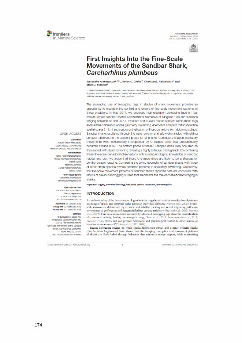
174