investigating local polarisation contrast with fibre …€¦ · axially in air, 1.6 µm...
TRANSCRIPT
i
INVESTIGATING LOCAL
POLARISATION CONTRAST WITH
FIBRE-BASED POLARISATION-
SENSITIVE OPTICAL COHERENCE
TOMOGRAPHY AND MICROSCOPY
Qingyun Li
BEng, MEng
This thesis is presented for the degree of
Doctor of Philosophy
of The University of Western Australia
Department of Electrical, Electronic & Computer Engineering
2020

ii
iii
In loving memory of my grandfather
Zhonghe Li
1922‒2019

iv

v
THESIS DECLARATION
I, Qingyun Li, certify that:
This thesis has been substantially accomplished during enrolment in this
degree.
This thesis does not contain material which has been submitted for the award
of any other degree or diploma in my name, in any university or other tertiary
institution.
In the future, no part of this thesis will be used in a submission in my name, for
any other degree or diploma in any university or other tertiary institution without
the prior approval of The University of Western Australia and where applicable,
any partner institution responsible for the joint-award of this degree.
This thesis does not contain any material previously published or written by
another person, except where due reference has been made in the text and,
where relevant, in the Authorship Declaration that follows.
This thesis does not violate or infringe any copyright, trademark, patent, or
other rights whatsoever of any person.
The research involving human and animal data reported in this thesis is
presented only as part of published work and work prepared for publication; the
relevant ethics approvals for each work are listed in the corresponding methods
sections.
This thesis contains published work and work prepared for publication, some
of which has been co-authored.

vi
Signature: Qingyun Li
Date: 26/03/2020

vii
ABSTRACT
This thesis makes several important contributions to polarisation-sensitive optical
coherence tomography (PS-OCT) through developing novel methods to
effectively extract local contrast from birefringence and the orientation of the
associated optic axis, at conventional and ultra-high resolution.
It has been challenging to retrieve the local optic axis (OA) orientation of the
sample in single-mode-fibre-based PS-OCT, due to the unknown transmission
matrices of the fibre circuits in the system. A robust method was developed that
is able to calculate the relative local OA in both bench-top and catheter-based
PS-OCT systems. The method corrects for the system polarisation distortions,
including both polarisation mode dispersion and polarisation-dependent loss in
the wavenumber domain, whilst maintaining the full axial resolution. Airway
samples from sheep and humans were scanned ex vivo, and the local OA clearly
demonstrated that the smooth muscle layer was orthogonal to the mucosal layer.
The ability to segment the smooth muscle layer from its surrounding tissues,
especially in a catheter-based scenario, can potentially allow in-vivo studies of
smooth muscle remodelling, a phenomenon of great significance in diseases
such as asthma.
The local birefringence, proportional to the scalar retardation of a local layer,
on the other hand, is more straightforwardly available. In-vivo measurements
were performed on human oral mucosa that demonstrated the depth-resolved
organisation of stromal collagen fibres. Furthermore, multi-contrast imaging was
demonstrated to afford a better understanding of the complex structure, by
viii
adding the angiographic contrast from speckle decorrelation, and coding the local
phase retardation (brightness) with local OA (colour).
Ultra-high-resolution (sub-2 m) imaging is desirable as it reveals micro-
morphology not available at more conventional resolutions. Incorporation of ultra-
high-resolution into local birefringence imaging improves the ability to resolve
micrometre-scale fibrous tissues in particular. PS-optical coherence microscopy
(OCM) with ultra-high-resolution and extended-focus was developed. The system
uses a Bessel beam for illumination and Gaussian beam for detection, that
breaks the intrinsic trade-off between lateral resolution and depth of focus in
Gaussian optics. The setup has an almost isotropic spatial resolution (1.4 µm
axially in air, 1.6 µm laterally), and an extended depth of focus (approximately
70 µm in tissue). The robust method to calculate the local OA, developed for fibre-
based PS-OCT, was also applied here, to correct for the system polarisation
distortions. Ocular tissues, including the limbus and cornea, from sheep, were
scanned ex vivo. As a result of the exceptional resolution, three-dimensional
distribution and organisation of the collagen fibre bundles in individual layers of
the cornea were clearly depicted in the volumetric local OA image.
Overall, the methods developed here show promise for a range of applications,
from understanding tumour progression in animal models, to assessment of
cancer, respiratory and other disease in humans.
ix
ACKNOWLEDGEMENTS
First, a sincere thanks to my supervisors for their guidance of my research: Prof.
David D. Sampson, Dr. Martin Villiger and Dr. Karol Karnowski. David offered me
the precious opportunity to pursue my dream PhD in OBEL and helped me
winning a scholarship to support my studies. Martin encouraged me to complete
my PhD in difficult times and brought lots of hope to my life, which I will remember
for the rest of my life. Karol quietly helped me with many things in both research
and life and supported me all the way towards the finishing line.
Many thanks to the other OBEL members: Dr. Andrea Curatolo, A/Prof. Barry
Cense, Dr. Peijun Gong, Michael Hackmann, Gavrielle Untracht, Danuta
Sampson, Liz Albert, Hava Zhang, Qiang Wang, including visitors Dr. Fabio
Feroldi, Tim Eixmann, Prof. Gijs van Soest.
Thanks also to my collaborators from other laboratories: Dr. Julia Walther, Dr.
Peter B. Noble, Prof. Alan James, Dr. Alvenia Cairncross, Prof. Camile S. Farah,
and Jonas Golde.
This research was supported by an Australian Government Research Training
Program (RTP) Scholarship. Travel grants from UWA Graduate Research School
to support attending international conferences are also acknowledged.
Last, but not least, I thank my parents for their endless support in my life, and
my fiancée, Ying, without whose company I would never be able to complete this
long journey.

x
STATEMENT OF CONTRIBUTION
This thesis contains the results of the research that I, Qingyun Li (QL), performed
within the Department of Electrical, Electronic, and Computer Engineering at The
University of Western Australia, between 2015 and 2020. Except where indicated
below and throughout the text, all work and writing are my own. The chapters of
this thesis are primarily derived from four full-length journal articles (3 published,
and 1 submitted): two first-authored, and two co-first-authored. I am the sole
author of the remainder of the document. Sections 3.1, 3.2, 4.1 and 5.1 are
reproductions of publications, as reported below, included without change in
content, but modified only in formatting for consistency with the remainder of this
document. I am the sole author of Chapters 1, 6 and the majority of Chapter 2
(except where indicated).
Listed below are the publications included in this thesis. My contributions are
given as a percentage next to my name, and in the descriptions.
1. Q. Li (40%), K. Karnowski, P. B. Noble, A. Cairncross, A. James, M.
Villiger, and D. D. Sampson, “Robust reconstruction of local optic axis
orientation with fiber-based polarization-sensitive optical coherence
tomography,” Biomedical Optics Express 9 (11), 5437-5455 (2018).
Section 4.1. QL was the principle author of this article. QL upgraded an
existing PS-OCT with KK and MV, programmed the acquisition and real-time
display software, performed the experiments with KK and PBN, developed the
processing chain under the supervision of MV, reviewed results and planned
xi
experiments with DDS, and composed the draft, which was edited and
reviewed by all co-authors.
2. J. Walther†, Q. Li† (25%), M. Villiger, C. S. Farah, E. Koch, K. Karnowski,
and D. D. Sampson, “Depth-resolved birefringence imaging of collagen
fiber organization in the human oral mucosa in vivo,” Biomedical Optics
Express 10 (4), 1942-1956 (2019).
Section 3.1. JW and QL were the joint principal authors of this article. JW and
QL adapted the system, performed the experiments and processed the data.
QL adapted the processing chain from MV, discussed the results and revised
the draft.
3. Q. Li (40%), K. Karnowski, G. Untracht, P. B. Noble, B. Cense, M. Villiger†,
and D. D. Sampson†, “Vectorial birefringence imaging by optical
coherence microscopy for assessing fibrillar microstructures in the cornea
and limbus,” Biomedical Optics Express 11 (2), 1122-1138 (2020).
Section 5.1. QL was the principle author of this article. QL designed the
system with MV, KK, and DS, established the system with MV, programmed
the data acquisition, hardware control and real-time display software, took the
measurements, improved the processing chain under the supervision of MV,
reviewed results and planned experiments with DDS, processed the data,
prepared the results under the supervision of MV and composed the draft,
which was edited and reviewed by all co-authors.
4. K. Karnowski†, Q. Li† (20%), A. Poudyal, M. Villiger, C. S. Farah, and D.
D. Sampson, “Influence of tissue fixation on depth-resolved birefringence
of oral cavity tissue samples,” Journal of Biomedical Optics (submitted).
Section 3.2. KK and QL were the joint principle authors of this article. KK and
QL optimised the system, performed the experiments and processed the data.
QL revised the draft.
Student signature: Qingyun Li

xii
Date: 26/03/2020
Coordinating supervisor signature: . . . . . . . . . . . . . . . . . . . . . . . . .
Date: 27/03/2020
xiii
LIST OF PUBLICATIONS
The following is a chronological list of publications arising during the duration of
this thesis.
Fully refereed journal articles
Key: † These authors contributed equally to this work
• Q. Li, K. Karnowski, P. B. Noble, A. Cairncross, A. James, M. Villiger,
and D. D. Sampson, “Robust reconstruction of local optic axis
orientation with fiber-based polarization-sensitive optical coherence
tomography,” Biomedical Optics Express 9 (11), 5437-5455 (2018).
• J. Walther†, Q. Li†, M. Villiger, C. S. Farah, E. Koch, K. Karnowski, and
D. D. Sampson, “Depth-resolved birefringence imaging of collagen
fiber organization in the human oral mucosa in vivo,” Biomedical Optics
Express 10 (4), 1942-1956 (2019).
• Q. Li, K. Karnowski, G. Untracht, P. B. Noble, B. Cense, M. Villiger†,
and D. D. Sampson†, “Vectorial birefringence imaging by optical
coherence microscopy for assessing fibrillar microstructures in the
cornea and limbus,” Biomedical Optics Express 11 (2), 1122-1138
(2020).
• K. Karnowski†, Q. Li†, A. Poudyal, M. Villiger, C. S. Farah, and D. D.
Sampson, “Influence of tissue fixation on depth-resolved birefringence
of oral cavity tissue samples,” Journal of Biomedical Optics (submitted).
xiv
Selected conference papers (First author only)
Key: * International | ^ Domestic | § Abstract| | ! Unrefereed or abstract refereed
1. *§! Q. Li, K. Karnowski, P. B. Noble, M. Hackmann, O. Çetinkaya, B.
Cense, A. James, M. Villiger, and D. D. Sampson, “Local optic axis
mapping for airway smooth muscle assessment in catheter-based
polarization-sensitive optical coherence tomography,” SPIE Photonics
West: Biomedical Optics and Biophotonics (BiOS), San Francisco, USA,
2 - 7 Feb. 2019.
2. ^§! Q. Li, K. Karnowski, P. B. Noble, M. Hackmann, O. Çetinkaya, B.
Cense, A. James, M. Villiger, and D. D. Sampson, “Local optic axis
mapping in bench-top and catheter-based polarization-sensitive optical
coherence tomography,” 15th Conference on Optics Within Life Sciences
(OWLS), Rottnest Island, Australia, 25 – 28 Nov. 2018.
3. *§! Q. Li, K. Karnowski, P. B. Noble, A. James, M. Villiger, and D. D.
Sampson, “Reconstruction of depth-resolved relative optic axis orientation
with passive delay polarization-multiplexed PS-OCT,” SPIE Photonics
West: Biomedical Optics and Biophotonics (BiOS), San Francisco, USA,
27 Jan. – 1 Feb. 2018.
4. ^§! Q. Li, K. Karnowski, M. Villiger, and D. D. Sampson, “Local
birefringence of the anterior segment of the human eye in a single capture
with full range polarization-sensitive optical coherence tomography,”
International Conference on Biophotonics, Perth, Australia, 30 Apr. – 1
May 2017 (Best poster award winner).
5. ^§! Q. Li, K. Karnowski, M. Villiger, D. Lorenser, and D. D. Sampson, “Full-
range complex swept-source polarization-sensitive optical coherence
tomography,” Biophotonics Australasia, Adelaide, Australia, 16 – 19 Oct.
2016.

xv
TABLE OF CONTENTS
Thesis Declaration
Abstract
Acknowledgements
Statement of Contribution
List of Publications
Table of Contents
Authorship Declaration
List of Figures
List of Acronyms
Chapter 1: INTRODUCTION …………………………………………...…….….1
1.1 Research objectives ………………………………………………..…….…..1
1.2 Structure of the thesis ……………………………………………….…..……2
Chapter 2: BACKGROUND ………………………………………………………4
2.1 Optical coherence tomography ……………………………………………....5
2.1.1 Working principle …………………………………………………......5
2.1.2 Imaging properties …………………………………………………..11
2.2 Polarisation-sensitive optical coherence tomography ……………..…….12
xvi
2.2.1 Fundamentals of polarisation ………………………………………12
2.2.2 PS-OCT configurations ………………………………………..…...19
2.2.3 Reconstructing tissue polarisation properties ……………………26
Chapter 3: LOCAL BIREFRINGENCE IMAGING ……………………………31
3.1 Depth-resolved birefringence imaging of collagen fiber organization in the
human oral mucosa in vivo ………………………………………………………32
3.1.1 Motivation …………………………………………………………….33
3.1.2 Methods ………………………………………………………………35
3.1.3 Experimental results ………………………………………………...41
3.1.4 Discussion and conclusion .………………………………………..48
3.2 Influence of tissue fixation on depth-resolved birefringence of oral cavity
tissue samples ……………………………………………………………..…….59
3.2.1 Introduction …………………………………………………..….…..60
3.2.2 Materials and methods……………………………………………….62
3.2.3 Results …………………………………………………………...…..66
3.2.4 Discussion and conclusions ………………………………………..69
3.3 Conclusion …………………………………………………………………….74
Chapter 4: LOCAL OPTIC AXIS IMAGING …………………………………...75
4.1 Robust reconstruction of local optic axis orientation with fiber-based
polarization-sensitive optical coherence tomography …………………………76
4.1.1 Introduction …………………………………………………………..77
4.1.2 Methods ………………………………………………………………79
4.1.3 Algorithm ……………………………………………………………..80
4.1.4 Results ……………………………………………………...………..89
xvii
4.1.5 Discussion ……………………………………………………………96
4.1.6 Conclusion …………………………………………………………..100
4.2 Rotating catheter-based configuration …………………………………...108
4.3 Full-range configuration ……………………………………………………112
4.4 Multi-functional PS-OCT …………………………………………………..117
4.5 Summary …………………………………..…………………….……….….120
Chapter 5: POLARIZATION-SENSITIVE OPTICAL COHERENCE
MICROSCOPY ………………………….…………………………...………….122
5.1 Vectorial birefringence imaging by optical coherence microscopy for
assessing fibrillar microstructures in the cornea and limbus…………………123
5.1.1 Introduction ………………………………………………..…….…124
5.1.2 Materials and methods ……………………………………………126
5.1.3 Results ……………………………………………………...…….…132
5.1.4 Discussion ………………………………………………………......142
5.1.5 Conclusion …………………………………………………………..146
5.2 Summary ………………………………………………………………….....155
Chapter 6: CONCLUSION AND PERSPECTIVES ………………………..156
6.1 Research contributions and significance ………………………………..156
6.2 Study limitations and future work ……………………………………..…158
6.3 Final remarks ……………………………………………………………….161
Bibliography …………………………………………………………..………162

xviii
AUTHORSHIP DECLARATION
This thesis contains work that has been published and prepared for
publication.
Details of the work:
Depth-resolved birefringence imaging of collagen fiber organization in the
human oral mucosa in vivo
Location in thesis:
Section 3.1
Student contribution to work:
Adapted the PS-OCT system, performed the experiment, processed the data,
discussed the results and revised the draft.
Details of the work:
Robust reconstruction of local optic axis orientation with fiber-based
polarization-sensitive optical coherence tomography
Location in thesis:
Section 4.1
Student contribution to work:
Upgraded an existing PS-OCT system, programmed the acquisition and
control software, performed the experiment, developed the algorithm,
processed the data, composed and revised the draft.
xix
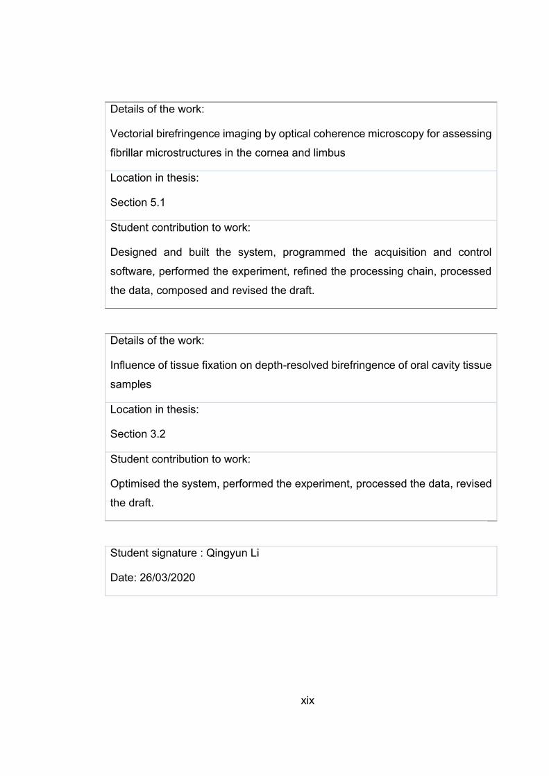
Details of the work:
Vectorial birefringence imaging by optical coherence microscopy for assessing
fibrillar microstructures in the cornea and limbus
Location in thesis:
Section 5.1
Student contribution to work:
Designed and built the system, programmed the acquisition and control
software, performed the experiment, refined the processing chain, processed
the data, composed and revised the draft.
Details of the work:
Influence of tissue fixation on depth-resolved birefringence of oral cavity tissue
samples
Location in thesis:
Section 3.2
Student contribution to work:
Optimised the system, performed the experiment, processed the data, revised
the draft.
Student signature : Qingyun Li
Date: 26/03/2020

xx
I, David D. Sampson, certify that the student’s statements regarding their
contribution to each of the works listed above are correct.
As all co-authors’ signatures could not be obtained, I hereby authorise inclusion
of the co-authored work in the thesis.
Coordinating supervisor signature:
Date: 27/03/2020
xxi
LIST OF FIGURES
2.1 A comparison of OCT resolution and penetration depth to other biomedical
imaging methods..………………………………………………………………6
2.2 Schematic of TD-OCT ………………………………………………………...7
2.3 Schematic of SD-OCT ………………………………………………………...8
2.4 Schematic of Michelson interferometry used in OCT..…………………..…10
2.5 A simple illustration of diattenuation and birefringence..……….…………..13
2.6 Poincaré sphere representation of Stokes vectors……………………..….18
2.7 Schematic of a basic setup of PS-OCT with one single input state..……..21
2.8 A conceptual scheme of the polarisation properties of the PS-OCT detecting
Jones matrices ……………………………………………………………......23
2.9 Simplified flowchart of processing for local polarisation contrasts in the
thesis …………………………………………………………………………...28
3.1 PS-OCT system with standard scanner head for imaging the oral mucosa
of the anterior human oral cavity in vivo ……………………………..……..36
3.2 Measurement points within the anterior oral cavity for representative
polarization-sensitive OCT imaging of the oral mucosa.…………………..38
3.3 Cross-sectional and en-face projection images of the labial oral mucosa by
PS-OCT..……………………………………………………………………….39
3.4 Averaged intensity and maximum intensity projection of the depth-resolved
birefringence (MIP Δn) of N = 30 en-face slices within the RL at
measurement point A in Fig. 3.2 (a), and the corresponding color depth-
encoded tissue birefringence…………………………………….…………..40
3.5 En-face projections of the intensity, depth-resolved birefringence and
cumulative retardation of the labial oral mucosa detected at position A in
Fig. 3.2 (a) and displayed via B-scans in Fig. 3.3 ……………………….…41
3.6 Intensity and birefringence (Δn) at different depths of the reticular layer (RL)
within the lamina propria of the inner side of the lower lip at measurement

xxii
points in Fig. 3.2 (a) labelled B (a) and C (c) presenting the vestibular
mucosa (mucolabial fold) (Fig. 3.2 (a)), and their corresponding color
depth-encoded depth-resolved birefringence ……………………………..43
3.7 Intensity and birefringence (Δn) at different depths of the dorsal tongue at
measurement points in Fig. 3.2(b) labelled D (a) and E (c), and their
corresponding color depth-encoded depth-resolved birefringence.……...44
3.8 Intensity and birefringence (Δn) at different depths of the transition region
from dorsal to lateral tongue at measurement points in Fig. 3.2(c) labelled
F (a) and G (c), and their corresponding color depth-encoded depth-
resolved birefringence ……………………………………………….…...…..46
3.9 Intensity and birefringence (Δn) at different depths of the transition from
dorsal to ventral tongue at measurement points in Fig. 3.2(c) labelled H (a)
and I (c), and their corresponding color depth-encoded depth-resolved
birefringence ……………………………………………...………….……….47
3.10 Intensity and birefringence (Δn) at different depths of the ventral tongue at
measurement points in Fig. 3.2(d) labelled J (a) and K (c), and their
corresponding color depth-encoded depth-resolved birefringence …..….48
3.11 Cross-sectional (B-scan) images of the ex vivo right ventral tongue
sample ………………..………………………………………………...……...64
3.12 Paired - OCT intensity on the left and birefringence on the right - en-face
projections of an ex vivo right ventral tongue sample at various
depths...………………...……………..………………………….……………66
3.13 Paired - OCT intensity on the left and birefringence on the right - en-face
projections of an ex vivo right soft palate sample at various
depths.………………………………………………………….…...………....67
3.14 Quantitative comparison of contrast change during the fixation process for
all measured samples……………………………………………….………..68
3.15 Change in fixed-sample contrast versus fresh sample versus depth …..…69
4.1 Example of symmetrization of full Jones matrix with an ex-vivo lamb trachea
sample …………………………………………………………………………83
4.2 Compensation of system polarization distortions …………….………...…86
4.3 Generation and spatial filtering of cumulative SO(3) …………...……….…87
4.4 Validation with custom-made birefringence phantoms……………….…....90
4.5 Local optic axis orientations with different system distortions ………….…91
4.6 Cross-sectional B-scan views of lamb tracheal samples measured ex
vivo ………………………………………………………………...……….…..93
xxiii
4.7 En face views of lamb trachea samples measured ex vivo …………..…...94
4.8 Human airway sample measured ex vivo …………………………………..96
4.9 A simple schematic of the home-made catheter with ball lens structure 109
4.10 Estimation of the transmission matrices of the system in a rotating catheter
configuration……………………………………………………………….…111
4.11 Porcine airway sample imaged with a catheter ex vivo………………….112
4.12 Sketch of probing beam geometry for full-range configuration.……….…114
4.13 Comparison of conventional and full-range OCT processing ……………115
4.14 Full-range PS-OCT measurement of the anterior segment of a porcine eye
globe ex vivo………………………………………………………….………116
4.15 Intensity, local optic axis orientation, and speckle decorrelation images at
different depths of a healthy adult human lower lip, measured with PS-OCT
in vivo …………………………………………………………………..……..119
5.1 System schematic of PS-OCM ……………………………………….…….129
5.2 Mean DOP and DI of ~10 times diluted coffee creamer with respect to the
lateral A-line sampling density………………………………….…………..134
5.3 A representative cross-sectional view (in the fast scanning direction, XZ) of
the intensity, local OA orientation, local retardation, and DI, of the corneal-
sclera limbus region of an adult sheep eye globe (Sample #1), imaged ex
vivo …………………………………………………………………………...136
5.4 Three representative cross-sectional views (in the slow scanning direction,
YZ) of the intensity and local OA orientation of Sample #1 ………………138
5.5 A representative B-scan view of the intensity and the local OA orientation
of the limbus region of an adult sheep eye globe (Sample #2), imaged ex
vivo ……………………………………………………………….…………...139
5.6 Cross-sectional views of intensity and local OA orientation of the anterior
stroma of the cornea of an ex-vivo adult sheep eye globe, in the fast and
slow scanning directions, respectively ……………………………………140
5.7 A representative cross-sectional view of the intensity and local optic axis
orientation of the posterior stroma of the dissected cornea from a sheep
eye globe, imaged at approximately the central region, from inside out ex
vivo ……………………..………………………………………...........…….141
5.8 A quantitative analysis of local OA orientation and local retardation in five
representative lamellae in the posterior stroma …………………………142
xxiv
LIST OF ACRONYMS
Acronym Definition
1D One dimensional
2D Two dimensional
3D Three dimensional
AFM Atomic force microscopy
ASM Airway smooth muscle
DI Depolarisation index
DOF Depth of field
DOP Degree of polarisation
DOPU Degree of polarisation uniformity
EOM Electro-optic modulator
FD-OCT Fourier-domain optical coherence tomography
FOV Field of view
FWHM Full-width at half-maximum
H&E Haematoxylin and eosin
LCI Low coherence interferometry
MZI Mach-Zehnder interferometer
NA Numerical aperture

xxv
OA Optic axis
OCM Optical coherence microscopy
OCT Optical coherence tomography
PBS Polarising beam splitter
PLM Polarised light microscopy
PMD Polarisation mode dispersion
PMF Polarisation-maintaining fibre
PSF Point-spread-function
PS-OCM Polarisation-sensitive optical coherence microscopy
PS-OCT Polarisation-sensitive optical coherence tomography
QWP Quarter-wave plate
SD Speckle decorrelation
SD-OCT Spectral-domain optical coherence tomography
SHG Second harmonic generation
SMF Single-mode fibre
SNR Signal-to-noise ratio
SS-OCT Swept-source optical coherence tomography
TD-OCT Time-domain optical coherence tomography
TEM Transmission electron microscopy


1
1 INTRODUCTION
1.1 RESEARCH OBJECTIVES
Birefringence is an intrinsic property of biological tissues that is directly related to
the arrangement of fibrous structures. Polarisation-sensitive optical coherence
tomography (PS-OCT) measures the polarisation state and intensity of the depth-
resolved back-scattered light from a sample. Cumulative retardation and
cumulative optic axis orientation are the two parameters most reported in the PS-
OCT literature. These two sources of contrast, however, represent the cumulative
effect of light propagation from the sample surface to a certain depth and back
again, and can be difficult to interpret when the sample is not homogeneous
versus depth. Local retardation and local optic axis orientation, as implied,
represent the contrasts at a local layer in depth free from the cumulative effects,
and are hence more physically meaningful and more easily interpretable.
Yet, the local parameters describing polarisation contrast are more difficult to
extract than the cumulative ones, especially the local optic axis orientation.
Single-mode-fibre (SMF) -based systems, are more convenient than bulk-optic
ones and may be used in endoscopic imaging, significantly extending their
potential applications. Local optic axis orientation achieved with a SMF-based
system, in particular, is capable of segmenting different tissue layers in hollow
organs based on the orientations of the fibrous structures, and is thus highly

2
desirable in airway imaging to differentiate the smooth muscle, and may be very
useful in gastrointestinal and cardiovascular applications.
Currently, most PS-OCT systems lack the resolution to resolve tissue
organisation on the micrometre length scale. Such organisation carries direct
implications for health and disease but remains difficult to assess in vivo. Optical
coherence microscopy (OCM) is capable of revealing the micro-morphology non-
destructively, but it is commonly based on the backscattering intensity only, and
thus lacks tissue specificity. It is of great interest if polarisation-sensitive capability
is added to OCM such that the local birefringence and optic axis orientation could
further reveal the organisation of fibrous structures, which is not possible with
only the back-scattering intensity.
The objectives of this thesis are to develop PS-OCT systems and processing
algorithms to investigate the sources of local polarisation contrast, and to
demonstrate the usefulness of the local polarisation contrast in different tissues.
1.2 THESIS STRUCTURE
The content of each chapter is briefly summarized. Where journal papers are
included, they are reproduced as published, including with original language (US-
English) and reference list. Other papers cited elsewhere are listed in the
Bibliography at the end of the thesis.
Chapter 2 Background
Chapter 2 provides an overview of PS-OCT, starting with a brief introduction of
the fundamentals and some basic properties of OCT, and followed by a brief
overview of fundamentals of polarisation, basic PS-OCT setups and processing
algorithm used in the thesis.
Chapter 3 Local birefringence imaging
Chapter 3 introduces two applications of local birefringence imaging: imaging the
collagen fibre organisations in the human oral mucosa in vivo, and studying the
effect of fixation onto the local birefringence of human oral biopsy samples ex
vivo.
3
Chapter 4 Local optic axis orientation imaging
Chapter 4 develops a robust method to calculate the local optic axis orientation
from a SMF-based PS-OCT, which is extended from standard bench-top to
rotating catheter and full-range configurations, respectively. The smooth muscle
could be segmented from its surrounding tissue in airway samples using the
algorithm, in both bench-top and catheter configurations. Multi-functional PS-
OCT is also demonstrated, that provides additional angiography contrast and
allows comprehensive understanding of the tissue by combining contrasts
generated by the collagen fibre organisation and blood vessels.
Chapter 5 Polarisation-sensitive optical coherence microscopy
Chapter 5 describes a micron-resolution, focus-extended PS-OCM, and its
application to characterize the microstructures of limbus and cornea of ex-vivo
adult sheep eye globes. The local optic axis orientation provides a striking
contrast between fibrous structures at different orientations.
Chapter 6 Summary
Chapter 6 summarizes the main outcomes of this thesis and concludes with a
discussion and final remarks.

4
2 BACKGROUND
In this thesis, polarisation-sensitive optical coherence tomography (PS-OCT) and
microscopy (PS-OCM) are the two imaging techniques employed to measure the
polarisation properties of the sample. Since these two techniques share the same
basic working principle and differ mostly in resolution, for brevity, here only PS-
OCT is introduced. This chapter provides a brief background of PS-OCT,
beginning with OCT.
5
2.1 OCT
2.1.1 Working principle
OCT is an optical imaging modality capable of non-invasively acquiring three-
dimensional (3-D) and high-resolution images of biological samples [1].
Analogous to detecting the sound echoes in ultrasonography, OCT illuminates
the sample with near-infrared light and detects the backscattered light that
represents a depth-resolved signal (A-line). A cross-sectional, two-dimensional
(2-D) image (B-scan) can be formed by translating the probing beam transversely
to the sample, and a sequence of B-scans can construct a volumetric, 3-D
dataset (C-scan). Since the speed of light is orders of magnitude faster than that
of sound, it is not feasible currently to measure the time-of-flight of light directly.
Instead, OCT uses coherence gating to resolve the time-of-flight of light and
hence the depth structure of sample, based on the technique of low coherence
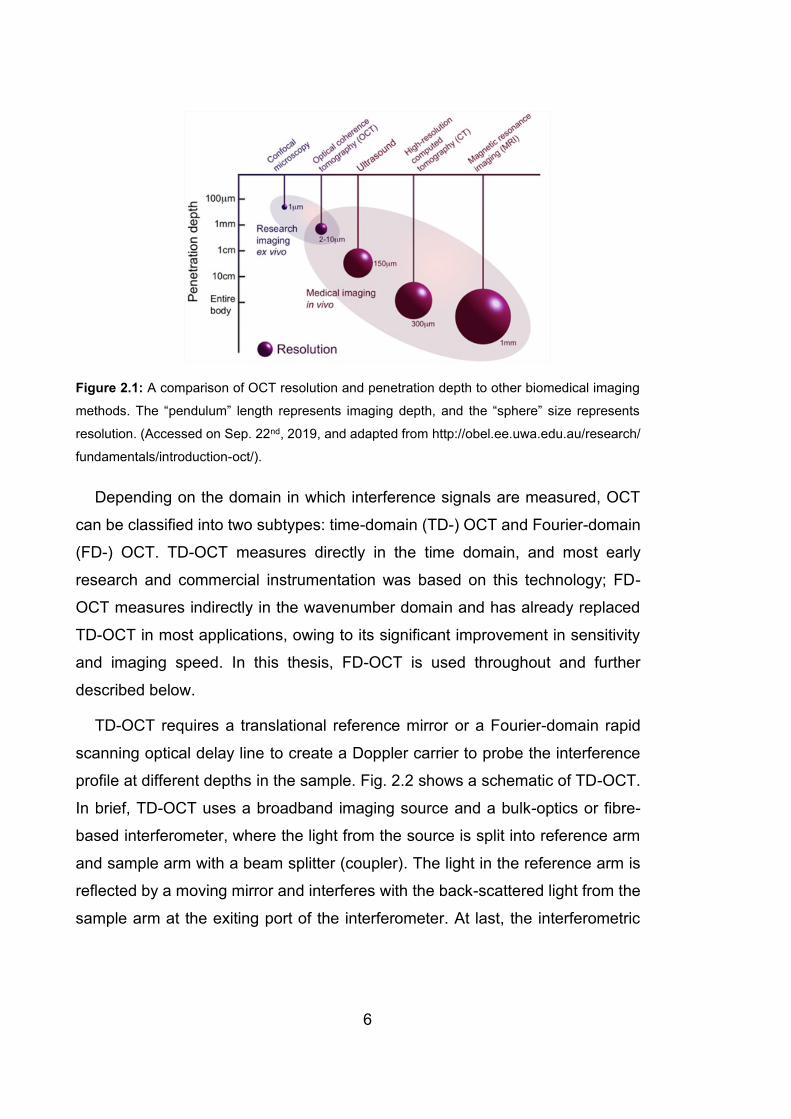
interferometry (LCI) [2]. A comparison of OCT resolution and penetration depth
to other biomedical imaging methods is presented in Fig. 2.1, which shows nicely
that OCT fills the gap between in-vivo medical imaging techniques and ex-vivo
microscopy.
6
Figure 2.1: A comparison of OCT resolution and penetration depth to other biomedical imaging
methods. The “pendulum” length represents imaging depth, and the “sphere” size represents
resolution. (Accessed on Sep. 22nd, 2019, and adapted from http://obel.ee.uwa.edu.au/research/
fundamentals/introduction-oct/).
Depending on the domain in which interference signals are measured, OCT
can be classified into two subtypes: time-domain (TD-) OCT and Fourier-domain
(FD-) OCT. TD-OCT measures directly in the time domain, and most early
research and commercial instrumentation was based on this technology; FD-
OCT measures indirectly in the wavenumber domain and has already replaced
TD-OCT in most applications, owing to its significant improvement in sensitivity
and imaging speed. In this thesis, FD-OCT is used throughout and further
described below.
TD-OCT requires a translational reference mirror or a Fourier-domain rapid
scanning optical delay line to create a Doppler carrier to probe the interference
profile at different depths in the sample. Fig. 2.2 shows a schematic of TD-OCT.
In brief, TD-OCT uses a broadband imaging source and a bulk-optics or fibre-
based interferometer, where the light from the source is split into reference arm
and sample arm with a beam splitter (coupler). The light in the reference arm is
reflected by a moving mirror and interferes with the back-scattered light from the
sample arm at the exiting port of the interferometer. At last, the interferometric

7
signals are detected, whose demodulated intensity is used to reconstruct the A-
line profiles.
Figure 2.2: Schematic of TD-OCT. TD-OCT, time-domain OCT. (Accessed on Sep. 22nd, 2019,
and adapted from http://obel.ee.uwa.edu.au/research/fundamentals/introduction-oct/)
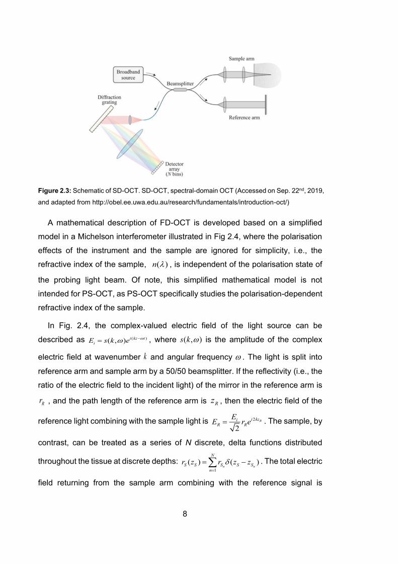
Similarly, FD-OCT also has two arms, i.e., the reference arm and the sample
arm. However, FD-OCT relaxes the need of translating the reference mirror and
hence enhances imaging speed. In this case, A-line profiles are not measured
directly in time domain, but reconstructed via Fourier transform of the acquired
interferometric signals in the wavenumber domain. Depending on the source type
and detection mechanism, FD-OCT can be further divided into two categories,
spectral domain (SD-) OCT and swept source (SS-) OCT. SD-OCT employs a
spectrometer to detect the spectral components of the interferometric signals,
whereas SS-OCT uses a wavelength tuning source such that the detected
spectral components are encoded in time. SS-OCT systems are more robust
because photodetectors are used to measure the interference signals, which
saves the efforts of aligning spectrometers. Yet, most high-resolution OCT
systems are based on SD-OCT, because commercial swept sources lack the
broad spectral bandwidth crucial for high-resolution imaging. In this thesis, the
measurements in Chapter 3 and Chapter 4 were based on a home-built SS-OCT
system, whereas the PS-OCM in Chapter 5 was a home-built SD-OCT instrument.
The schematic of SD-OCT is shown in Fig. 2.3.
8
Figure 2.3: Schematic of SD-OCT. SD-OCT, spectral-domain OCT (Accessed on Sep. 22nd, 2019,
and adapted from http://obel.ee.uwa.edu.au/research/fundamentals/introduction-oct/)
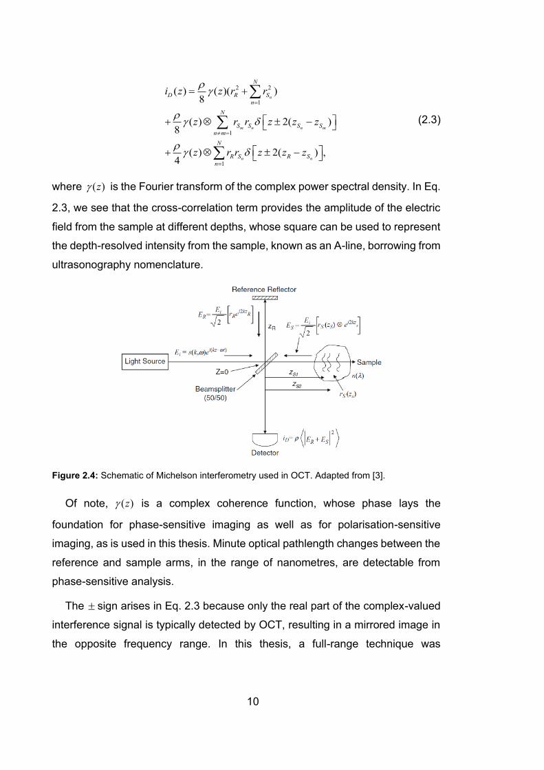
A mathematical description of FD-OCT is developed based on a simplified
model in a Michelson interferometer illustrated in Fig 2.4, where the polarisation
effects of the instrument and the sample are ignored for simplicity, i.e., the
refractive index of the sample, ( )n , is independent of the polarisation state of
the probing light beam. Of note, this simplified mathematical model is not
intended for PS-OCT, as PS-OCT specifically studies the polarisation-dependent
refractive index of the sample.
In Fig. 2.4, the complex-valued electric field of the light source can be
described as ( )( , ) i kz t
iE s k e −= , where ( , )s k is the amplitude of the complex
electric field at wavenumber k and angular frequency . The light is split into
reference arm and sample arm by a 50/50 beamsplitter. If the reflectivity (i.e., the
ratio of the electric field to the incident light) of the mirror in the reference arm is
Rr , and the path length of the reference arm is Rz , then the electric field of the
reference light combining with the sample light is 2
2
Ri kziR R
EE r e= . The sample, by
contrast, can be treated as a series of N discrete, delta functions distributed
throughout the tissue at discrete depths: 1
( ) ( )n n
N
S S S S S
n
r z r z z=
= − . The total electric
field returning from the sample arm combining with the reference signal is
9
2( )
2
Si kziS S S
EE r z e =
, where represents convolution. By substituting ( )S Sr z ,
one can simplify the description of the sample signal to 2
12
Sn
n
Ni kzi
S S
n
EE r e
=
= . The
photocurrent, DI , generated by the detector is given by:
2
,2
R S
D
E EI
+= (2.1)
where is the responsivity of the detector. The factor of 2 is to account for the
second pass of the beamsplitter, and denotes integration over the response
time of the detector. After substituting SE and RE , we can rewrite Eq. 2.1 as
below:
2 2
1
1
1
( ) ( )( )4
( ) cos 2 ( )4
( ) cos 2 ( ) ,2
n
m n n m
n n
N
D R S
n
N
S S S S
n m
N
R S R S
n
I k S k r r
S k r r k z z
S k r r k z z
=
=
=
= +
+ −
+ −
(2.2)
where 2
( ) ( , )S k s k = is the power spectral distribution of the light source. The
first summand on the right-hand side (RHS) of Eq. 2.2 contains no interference
signal and is usually taken as the DC term. The second summand is the
interference signal of the sample from different depths, and is called auto-
correlation term. And the last summand is the desired interference signal
between the reference arm and the sample arm, and is called the cross-
correlation term. The first two terms do not contribute to OCT signals, and are not
even detected in SS-OCT when balanced detection is employed.
If we Fourier transform Eq. 2.2, we obtain the following:
10
2 2
1
1
1
( ) ( )( )8
( ) 2( )8
( ) 2( ) ,4
n
m n n m
n n
N
D R S
n
N
S S S S
n m
N
R S R S
n
i z z r r
z r r z z z
z r r z z z
=
=
=
= +
+ −
+ −
(2.3)
where ( )z is the Fourier transform of the complex power spectral density. In Eq.
2.3, we see that the cross-correlation term provides the amplitude of the electric
field from the sample at different depths, whose square can be used to represent
the depth-resolved intensity from the sample, known as an A-line, borrowing from
ultrasonography nomenclature.
Figure 2.4: Schematic of Michelson interferometry used in OCT. Adapted from [3].
Of note, ( )z is a complex coherence function, whose phase lays the
foundation for phase-sensitive imaging as well as for polarisation-sensitive
imaging, as is used in this thesis. Minute optical pathlength changes between the
reference and sample arms, in the range of nanometres, are detectable from
phase-sensitive analysis.
The sign arises in Eq. 2.3 because only the real part of the complex-valued
interference signal is typically detected by OCT, resulting in a mirrored image in
the opposite frequency range. In this thesis, a full-range technique was
11
demonstrated that removed the mirror artefact and doubled the usable imaging
range. This was achieved by performing an additional demodulation in the spatial
domain.
2.1.2 Imaging properties
Unlike most other microscopies, OCT systems have decoupled axial and lateral
resolving mechanisms, determined by the coherence gating and confocal gating
(focussing), respectively. The axial resolution, indicated by the coherence length
cl , is defined as the full-width at half-maximum (FWHM) of the axial point-spread-
function (PSF), and is determined purely by the central (mean) wavelength and
the effective spectral bandwidth of the imaging light source, given by:
2
02ln 2,cl
=
(2.4)
where and 0 represent the FWHM bandwidth and the central wavelength of
the light source, respectively. Here the spectrum of the source is assumed to be
of Gaussian shape. In practice, the spectrum of the imaging light source might
not have a perfect Gaussian shape, and reshaping the spectrum before
performing Fourier transformation is needed to maintain the nominal axial
resolution and minimize sidelobes in the point-spread function.
The lateral resolution and the depth of field (DOF), in contrast, are completely
determined by the focusing properties of the probing beam, in common with other
microscopic techniques. Using standard Gaussian optics, there exists an
inherent trade-off between lateral resolution and DOF, i.e., the higher the
numerical aperture (NA) of the imaging optics, the better the lateral resolution,
and the shorter the DOF. For high lateral resolution (< 2 μm) OCT systems, the
nominal DOF is less than 30 μm, limiting the capacity of imaging in depth. This is
because FD-OCT captures a full A-line in a single sweep, and thus a strong focal
gate is inefficient, as the remainder of the sweep/energy is thrown away. A simple
and straightforward way to overcome this limitation is to physically translate the
12
confocal gate for depth sectioning, as is done in full-field (FF-) OCM [4] and
Gabor-domain OCT [5]. However, this strategy does not satisfy our needs for PS-
OCM imaging because: firstly, acquiring multiple depths to reconstruct a full B-
scan requires more time, limiting the capability for in-vivo applications; secondly,
any mechanically moving part in the instrument will tend to cause deterioration of
the phase sensitivity of the system, preventing us from reaching SNR-limited
phase sensitivity [6].
In contrast to Gaussian beams, Bessel-like beams can maintain a high lateral
resolution over an extended DOF, at the cost of system sensitivity loss [7], which
can be partially compensated by increasing the power of the incident beam and
sidelobes in the point-spread function. In this thesis, a PS-OCM instrument was
built with engineered wavefront to maintain high lateral resolution over an
extended focus, by taking advantage of decoupled Bessel beam for illumination
and Gaussian beam for detection [8].
2.2 PS-OCT
Conventional OCT images are based on the back-scattering intensity which often
reveals morphology, but lacks specificity to tissue type. Polarisation-sensitive
optical coherence tomography (PS-OCT) is one important contrast extension of
OCT, in that it additionally measures the polarisation properties of the sample,
which are related to the organisation of the fibrous structures it contains.
In this section, before introducing our processing algorithm, we first briefly
touch on the fundamentals of polarisation, and describe basic PS-OCT setups.
2.2.1 Fundamentals of polarisation
Longitudinal waves, such as sound in a gas or liquid, can be completely
described by their amplitude, frequency and phase. However, the same
parameters are not adequate to fully characterise transverse waves, such as
electromagnetic waves, in that transverse waves have an additional freedom in
the direction of oscillations, known as the state of polarisation. In our previous
mathematical models in Section 2.1, light has been assumed to be linearly

13
polarised and the refractive index of the sample to be independent of the
polarisation state of the incident light. Whilst such a simplified model is enough
for most OCT techniques, it does not satisfy the needs of PS-OCT, which
specifically seeks to ascertain the polarisation-dependent effect of a sample on
the incident beam.
The real and imaginary parts of the complex-valued refractive index of a
medium determine, respectively, the phase velocity and attenuation of light as it
propagates through the medium. If the real part of the refractive index of a
medium is dependent on the polarisation state of the light, this medium is
birefringent; whereas, if the imaginary part is dependent on the polarisation state
of the light, the medium is diattenuating.
Although birefringent materials exhibit optical properties dependent on the
polarisation state of light, there is at least one propagation axis in the material,
along which light travels always at a constant phase velocity, regardless of its
polarisation state. This axis is called optic axis, and depending on the number of
optic axes, birefringent materials can be classified into uniaxial and biaxial forms,
representing those with a single optic axis and two optic axes, respectively.
Figure 2.5: A simple illustration of diattenuation (left) and birefringence (right). In the illustration,
for diattenuation, the intensity of the electric field is attenuated by different amounts in the
horizontal and vertical directions; whereas, for birefringence, the phase velocity of the electric
field is different in the horizontal and vertical directions, leading to a relative phase delay between
the fields in the two directions. Adapted from [9].
In uniaxial media, the real part of the refractive index for polarised light aligned
parallel to the optic axis (extraordinary ray) is en , whereas the real part of the

14
refractive index for polarised light aligned perpendicular to the optic axis (ordinary
ray) is on . The difference between these two refractive indices, en and on , defines
the magnitude of birefringence of this medium, e on n n = − . A phase retardation
, will be induced between the extraordinary and ordinary rays of light passing
through a birefringent material, whose amount is given by:
,n L k = (2.5)
where L is the length light travels in the medium, and k is the wavenumber of the
light. Eq. 2.5 links between phase retardation and the scalar amount of
birefringence. PS-OCT measures the phase retardation and converts that to
birefringence.
Biological samples usually exhibit negligible diattenuation, and birefringence
and depolarisation are the more pronounced polarisation properties interesting
to study by PS-OCT. Birefringence arises from the arrangement of fibrous
structures in the sample, and the observed birefringence might be a combination
of both intrinsic and form birefringence. Biological birefringent tissues, such as
collagen and muscle, feature positive birefringence [10], and hence, the axis of
the fibres is the slow axis, i.e., the polarised light whose polarisation state is
parallel to the fibre axis has the lowest phase velocity, whereas the light whose
polarisation state is perpendicular to the fibre axis has the highest phase velocity.
Hence, the fast axis orientation measured by PS-OCT is perpendicular to the true
axis of the fibres [11].
Jones calculus is a convenient formalism for describing purely polarised light
and the non-depolarising polarisation properties of media, i.e., the polarisation
state of purely polarised light can be expressed by a complex-valued column
Jones vector E , and the non-depolarising properties of any optical element or
system by a 2 × 2 complex-valued Jones matrix J . The output polarisation state
E of an input polarisation state E , after transmitting through an optical system
with a Jones matrix J , is determined by:

15
11 12
21 22
,H H
V V
E EJ J
E EJ J
= = = E JE (2.6)
where T
H VE E and T
H VE E denote the complex electric fields of the input
and output light in two orthogonal directions (horizontal and vertical)
perpendicular to the propagation direction of the light. A Jones matrix describes
fully the non-depolarising properties of a material, and it is feasible to extract
these properties by analysing the Jones matrix of a material. For instance, the
phase retardation between the ordinary and the extraordinary rays, and the optic
axis orientation, are encoded in the eigenvalues and the eigenvectors of the
Jones matrix, respectively.
The combined or cumulative, non-depolarising polarisation effect totJ of a
series of optical elements, 1J , 2J , 3J ,···, nJ , is their product:
tot 1 2 1.n n−= J J J J J (2.7)
Of note, biological samples can be treated as a multiple-layer structure, and
each local layer has its local non-depolarising property also representable by a
Jones matrix. Ignoring the system transmission matrices, PS-OCT directly
measures the round-trip matrix from sample surface to a certain depth and back,
that essentially describes a round-trip cumulative matrix. Here, Eq. 2.7 provides
us the hint to access the local matrix from the cumulative matrix, i.e., remove the
matrix of preceding layers from the cumulative matrix.
Since Jones formalism can only deal with purely polarised light, Mueller-
Stokes formalism is needed where the depolarising properties of light and sample
are of interest. In analogy to a Jones vector, a Stokes vector can describe the
polarisation state of light, which is composed of four real-valued elements,
, , ,T
I Q U V , and defined by a set of irradiance measurements, given by:

16
* *
* *
0 90
* *
45 45
* *( ) ,
tot H H V V
H H V V
H V V H
rc lc H V V H
I I E E E E
Q I I E E E E
U I I E E E E
V I I i E E E E
−
−
= = +
= − = −
= − = +
= − = − −
(2.8)
where HE and VE denote the horizontal and vertical electric field of a Jones
vector, respectively. is an ‘ensemble’ average over time or space. Here I is
the overall irradiance of the beam, and Q is the difference of the irradiance of the
beam between 0˚ and 90˚. In analogy, U and V are the differences of irradiance
between 45˚ and -45˚, right and left circular polarisations, respectively.
The degree of polarisation (DOP) is needed to describe partially polarised light,
defined as:
2 2 2
2,
Q U VDOP
I
+ += (2.9)
which ranges from 0 for completely unpolarised light, to unity for purely polarised
light. For depolarisation imaging, most PS-OCT literatures detect Jones vectors,
convert them to Stokes vectors, perform spatial averaging and analyse the
depolarisation property. Of note, since PS-OCT is a coherent imaging technique,
the DOP calculated from those directly derived Stokes vectors remains unity. It
is by spatial averaging of the Stokes vectors over a few speckles that one gains
access to the degree of polarisation uniformity (DOPU) [12], which is closely
related to the definition of DOP.
In analogy to Jones vectors, the evolution of a Stokes vector through an optical
system or element, can also be described mathematically by applying a matrix
that contains the polarisation properties of the optical component:

17
11 12 13 14
21 22 23 24
31 32 33 34
41 42 43 44
'
'' .
'
'
M M M MI I
M M M MQ QS S
M M M MU U
M M M MV V
= = =
M (2.10)
Here, the 4 × 4 real-valued matrix, M , is named Mueller matrix. A Mueller
matrix has advantages over a Jones matrix of being able to describe all the
possible polarisation effects, including depolarisation, of the optical elements.
According to the definition, direct measurements of the full Mueller matrix
require a total of 16 measurements, which is too many and impractical for in-vivo
PS-OCT imaging [13]. Yet, efforts can be significantly saved by measuring a
Jones matrix and converting it to a Mueller matrix. A straightforward way to
transfer a Jones matrix to its corresponding Mueller matrix is given by [14]:
* 1( ) ,
1 0 0 1
1 0 0 1where = .
0 1 1 0
0 0i i
−=
−
−
M U J J U
U (2.11)
Here J is the Jones matrix, * the complex conjugate operation, and ⨂ the
Kronecker tensor product. For 2 × 2 matrices, the Kronecker tensor product is
given by:
11 11 11 12 12 11 12 12
11 12 11 12 11 21 11 22 12 21 12 22
21 22 21 22 21 11 21 12 22 11 22 12
21 21 21 22 22 21 22 22
.
a b a b a b a b
a a b b a b a b a b a b
a a b b a b a b a b a b
a b a b a b a b
=
(2.12)
Since Jones matrices are non-depolarising, the Mueller matrices directly
derived from Jones matrices are also non-depolarising, and it is also by means
of spatial averaging the Mueller matrices over a few speckles that the
depolarisation properties can be retrieved.

18
The Q , U and V components of the Stokes vector are already enough to
describe the polarisation state of purely polarised light, whereas the I
component only provides the additional DOP information for partially polarised
light. Hence, the Stokes vectors in PS-OCT context can be simplified to three
components by normalising the parameters with I and dropping the normalised
component I , which is always unity after normalisation. The other three
parameters remaining, Q , U and V , can be represented as a vector in a
Poincaré sphere, which is a convenient yet useful geometrical tool for displaying
3D vectors. In the context of polarisation optics, Poincaré sphere is useful to
describe Stokes vectors and their evolution through materials. If the radius of the
Poincaré sphere is unity, a normalised Stokes vector of purely polarised light will
lie on the surface of the sphere, whereas a normalised Stokes vector of partially
polarised light will lie inside the sphere.
Figure 2.6: Poincaré sphere representation of Stokes vectors. Adapted from [15].
If a Mueller matrix contains only retardation components, all the meaningful
information of this Mueller matrix is contained in its lower right 3 × 3 sub-matrix.
In this case, this sub-matrix can be visualised as an operator that rotates any
normalised Stokes vectors in the Poincaré sphere along a common axis without
changing their lengths. Such a 3 × 3 matrix belongs to a 3-dimensional special
orthogonal group, SO(3), which is defined as the set of rotations:

19
3 3
3 3SO(3) I ,det( ) 1TR R R R
= = = (2.13)
Apparently, a SO(3) matrix, R , has only two rotational properties: the rotation
axis with a unit length 1 2 3ˆ , ,
Tr r r r= and the rotation angle , corresponding to
the axis and the amount of the rotation, respectively. Indeed, it is possible to
describe the two properties simultaneously using a single 3 × 1 vector r ,
whose axis and length represents the axis and amount of rotation, respectively.
These properties lay the foundation of vectorial birefringence, which can encode
simultaneously the scalar amount of phase retardation and the optic axis
orientation in a single 3 × 1 vector. In such a vectorial birefringence vector, the
axis and the length represent the optic axis orientation and the scalar amount of
phase retardation, respectively. In the following chapters of the thesis, the
advantage of encoding the optic axis orientation over the traditional scalar
amount of phase retardation is demonstrated. Mathematically, a rotation matrix,
R, is linked with its rotation properties by [16]:
ˆˆ ˆ(cos ) (1 cos ) (sin ) ,R I rr r = + − + (2.14)
where the 3-D dyadic ˆˆrr is the projection operator and r the cross-product
operator:
1 1 1 2 1 3 3 2
2 1 2 2 2 3 3 1
3 1 3 2 3 3 2 1
0
ˆˆ ˆ; 0 .
0
r r r r r r r r
rr r r r r r r r r r
r r r r r r r r
−
= = − −
(2.15)
The link between a rotation matrix and its associated rotation vector, provides
the possibility to construct a rotation matrix based on a rotation vector, as well as
to decompose a rotation matrix into a rotation vector.
2.2.2 PS-OCT configurations
The A-scan element of PS-OCT was first demonstrated by Hee at al. [17] in a
bulk-optic time-domain configuration in one dimension, shortly after the same
research group coined the term OCT. In this paper, for the first time, a polarisation
detection mechanism using two orthogonal polarisation channels was developed

20
and enabled measurement of the Jones vector, and hence the Stokes vector of
the back-scattered light. The first 2D (B-scan) PS-OCT image of a biological
sample required another 5 years to be demonstrated [18]. Since then, PS-OCT
technology has matured gradually, following closely the evolution of OCT, from
time-domain to Fourier-domain, and from simple bulk-optic-based to more
convenient fibre-based.
PS-OCT can be generally categorised into two basic formats, according to the
number of input states: single and double. With a single input state, usually
circularly polarised light is used to probe the sample; whereas, with double input
states, the polarisation states of the probing beam can be arbitrary (non-singular).
The former needs to measure only one Jones vector, whereas the latter needs
to measure two Jones vectors that can be combined to form a full Jones matrix,
or Stokes vector pairs. The single input state scheme is typically implemented via
bulk-optic (or polarising-maintaining fibre-based) systems, where the
transmission matrix of every component is known, and the double input state
scheme is employed by SMF-based systems, where the transmission matrices
of the fibres are unknown.
Compared to bulk-optics and polarisation-maintaining fibre-based systems,
SMF-based systems are flexible in handling, robust in alignment and effective in
cost, and hence, they are more promising for in-vivo clinical applications.
Fig. 2.7 shows a simplified schematic of single-input-state bulk-optic PS-OCT
system. The linear polariser in the source port filters the light such that only the
polarised light in the horizontal direction passes through to the beam splitter,
which splits the light into reference arm and sample arm, the same way as in
conventional OCT. Yet, the reflected light from the reference arm is no more
horizontal, but diagonal, because it travels a round-trip through the quarter wave
plate (QWP1) orientated at 22.5˚ with respect to the horizontal direction. The
reference light is diagonally polarised to ensure that it has equal amplitude and
phase in both horizontal and vertical directions, and the contribution of the
reference light to the interference signals can be simplified to a common scalar
21
that amplifies the sample signal. The polarisation state of the light in the sample
arm is converted from linear to circular by QWP2, the axis of which is orientated
at 45˚ relative to the horizontal direction. The back-scattered light from the sample,
usually in an elliptical polarisation state, is recombined with the reference signal
at the exit port and divided by a polarising beam splitter and detected by two
separate detectors.
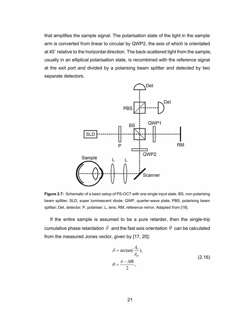
Figure 2.7: Schematic of a basic setup of PS-OCT with one single input state. BS, non-polarising
beam splitter; SLD, super luminescent diode; QWP, quarter-wave plate; PBS, polarising beam
splitter; Det, detector; P, polariser; L, lens; RM, reference mirror. Adapted from [19].
If the entire sample is assumed to be a pure retarder, then the single-trip
cumulative phase retardation and the fast axis orientation can be calculated
from the measured Jones vector, given by [17, 20]:
arctan( ),
,2
V
H
A
A
=
− =
(2.16)
22
where VA and HA are the amplitudes of the electrical field in the vertical and
horizontal directions, respectively, and is the phase difference between them.
The main advantage of the first-generation bulk-optic PS-OCT lies in its simple
setup, i.e., only few additional changes are made from a standard bulk-optic OCT
system. However, this setup also has limitations. Firstly, bulk-optic systems are
less flexible and require more effort to maintain alignment and are difficult to
adapt for endoscopic imaging with catheters. Secondly, the fast axis indicates the
overall axis accumulated from the sample surface to a certain depth, and
corresponds to the true axis of the sample only when the sample does not have
a depth-varying optic axis, and the phase retardation is not wrapped [21].
However, in practice, these two conditions are difficult to meet in biological
samples, especially the former. Thirdly, in theory, there are possibilities that the
polarisation state of the probing beam inside the sample becomes aligned with
or perpendicular to the optic axis of the sample, in which case, no birefringence
would be detectable. Although using a circularly polarised probing beam already
minimises the chance of detection failure, it is not guaranteed.
Although most literature demonstrates only cumulative polarisation contrast
with such a setup, the researchers at the University of Missouri extracted local
polarisation contrast with the same setup [21, 22], by assuming that each local
layer is a linear retarder.
In terms of convenience of alignment, a fibre-based system would be a better
option, because it can divide the whole system into several sub-units, whose
alignment can be individually optimised without impacting each other.
Polarisation-maintaining fibre-based (PMF-based) PS-OCT systems [23], in
principle, can be treated as bulk-optic systems, but the fibres require careful
alignment of their optic axes with linearly polarised light, are also less cost-
effective [24] and prone to causing cross-talk artefacts [25]. PMF-based systems
also remain challenging for endoscopic applications, particularly when used with
rotational side-viewing imaging probes interfaced through a rotary joint. In
contrast, single-mode fibre-based systems relax the need for rotational alignment
23
of the fibres with respect to specific polarisation states. Yet, single-mode fibres
behave like retarders whose optic axis and birefringence change with
temperature and external mechanical forces. Furthermore, a circulator or a fibre
coupler is needed in the sample arm to link the sample arm with the light source
and the detection unit. In either case, the fibre segments delivering the source
light and connecting the sample arm with the detection unit introduces two distinct,
unknown polarisation transformations that sandwich the effect of the sample,
making it challenging to isolate the polarisation properties of the sample. In
general, probing the sample with only a single polarisation state is insufficient to
extract the polarisation properties of the sample, even if the sample and the fibres
are assumed to be pure retarders. However, recent developments towards single
input PS-OCT have overcome this limitation by leveraging the PMD of the system
[26].
A general conceptual scheme of an SMF-based PS-OCT systems is shown in
Fig. 2.8. There exist a variety of implementations to measure the desired matrices,
differing from each other mostly in the way two probing states are launched and
detected. To probe the sample with two incident polarisation states can be
achieved either sequentially [27] or simultaneously [28, 29]. In the former, a
polarisation modulator alternates the polarisation state of the source A-line by A-
line, whereas the latter multiplexes the two polarisation states along depth. The
simultaneous implementation requires an extended detection range and has so
far only been demonstrated with SS-OCT for several reasons. Firstly, the imaging
range of SS-OCT is relatively easy to extend, by electronically frequency doubling
the k-clock [30, 31], or directly a doubling the pathlength difference of the k-
clock’s Mach-Zehnder interferometer (MZI). Secondly, SS-OCT usually has a
smaller sensitivity roll-off along depth, thanks to the narrow instantaneous line-
width of the swept-source that leads to a longer instantaneous coherence length.

24
Figure 2.8:. A conceptual scheme of the polarisation properties of the PS-OCT detecting Jones
matrices. Here, Jin and Jout represent the matrices of the illumination and detection optics,
respectively. Js and JsT represent the cumulative matrix from sample surface to a certain depth,
and its return trip, respectively. Adapted from [32].
Despite the different implementations, eventually, all these systems lead to a
Jones matrix tomogram, representing the round-trip through the sample
sandwiched by two unknown system matrices, given by:
,T T
out in out s s in in out s s in= = =E JE J J J J E J J J J (2.17)
where (1) (2) (1) (2), , .out out out in in in in in inE E E E→ → → →
=
E E J J E The unknown system
transmission matrices might not only come from the optical fibres, but also the
rest of the optical elements [33, 34]. Hence, although optical fibres are generally
assumed as pure retarders [35], the overall system transmission matrices are not
necessarily pure retarders. There are several instances where diattenuation is
introduced into the measured Jones matrix, to name a few, the difference of the
irradiances of the two probing beams, and the difference of the coupling efficiency
and quantum efficiency of the photodetectors in the orthogonal detection
channels. Not only are the system matrices general Jones matrices, they may
also not be constant over the full spectrum, but vary with the wavenumber, which
is treated by us as system polarisation distortions. The sources of system
polarisation distortions include polarisation mode dispersion (PMD) [36], and the
wavelength-dependent diattenuation of the optical components. The system
25
polarisation distortions could lead to artefacts [37], if they are strong and not
compensated [38].
Starting from here, two different approaches have been developed to analyse
the sample birefringence properties, based either on Stokes vector analysis [39]
or the full Jones/Mueller matrix [35], via geometric reasoning and matrix
decomposition, respectively. Currently, the Jones matrix-based approach
appears to be the most commonly used analysis for PS-OCT, mostly because it
is more straightforward to calculate, and more tolerable to the exact relation of
the two probing polarisation states.
The introduction of Jones matrix method to analyse the PS-OCT
measurements is of high benefit to the evolution of PS-OCT, as the existing
theory and knowledge of Jones matrix formalism, as well as Mueller formalism,
can be directly applied to PS-OCT measurements. Many researchers even
directly call such PS-OCT systems Jones-matrix (PS-) OCT [33, 40], highlighting
the importance of recovering the full Jones matrix. The possible failure to detect
tissue birefringence due to the usage of a single input state that happens to be
aligned with or perpendicular to the optic axis of the sample, does not exist for
Jones matrix PS-OCT, because the difference of the phase delay between the
two unaltered probing states is still detected and encoded in the Jones matrix.
In principle, all the non-depolarising polarisation effects of a material could be
retrieved from its Jones matrix, as has been demonstrated with bulk-optic Jones-
matrix PS-OCT [11, 41-44]. Yet, the Jones matrix tomograms measured with
SMF-based PS-OCT systems also include two unknown system transmission
matrices that complicate the analysis of the sample property, especially the optic
axis orientation. Efforts have been made by different research groups to recover
the optic axis orientation [45, 46] from the cumulative matrix, assuming that the
sample has a constant optic axis over depth. Yet, the recovered optic axis
orientation is relative to an unknown laboratory frame and also ambiguous in sign,
and an additional calibration is thus needed to retrieve the absolute optic axis,
removing any ambiguity [47]. Indeed, the ambiguity of sign and laboratory frame
26
is inherent to all SMF-based PS-OCT systems, unless it is calibrated by a
birefringent sample with known optic axis orientation.
The optic axis orientation and the birefringence measured with PS-OCT both
correspond to the in-plane values, i.e., only the components projected onto the
plane perpendicular to the probing beam can be measured, in analogy to the
Doppler phase shift measured with Doppler OCT. If the optic axis of the sample
were parallel to the propagation direction of the probing beam, then no
birefringence would be detected. To recover the full three dimensional orientation
of the optic axis, corresponding, e.g. to a sample with fibrous tissue elements
oriented in all directions, requires at least two scans at different illumination
angles to measure two distinct projections of the optic axes and indirectly
conclude on its axial component [48, 49].
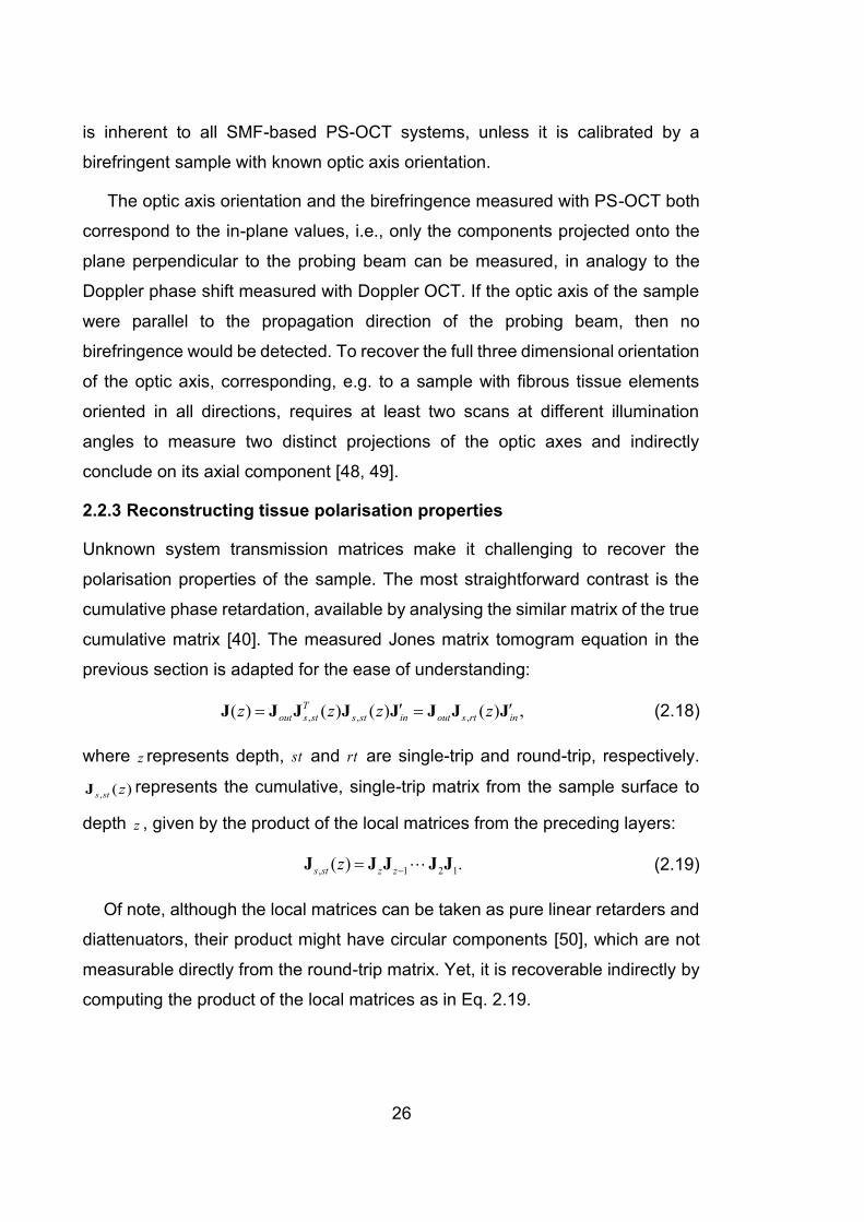
2.2.3 Reconstructing tissue polarisation properties
Unknown system transmission matrices make it challenging to recover the
polarisation properties of the sample. The most straightforward contrast is the
cumulative phase retardation, available by analysing the similar matrix of the true
cumulative matrix [40]. The measured Jones matrix tomogram equation in the
previous section is adapted for the ease of understanding:
, , ,( ) ( ) ( ) ( ) ,T
out s st s st in out s rt inz z z z = =J J J J J J J J (2.18)
where z represents depth, st and rt are single-trip and round-trip, respectively.
, ( )s st zJ represents the cumulative, single-trip matrix from the sample surface to
depth z , given by the product of the local matrices from the preceding layers:
, 1 2 1( ) .s st z zz −= J J J J J (2.19)
Of note, although the local matrices can be taken as pure linear retarders and
diattenuators, their product might have circular components [50], which are not
measurable directly from the round-trip matrix. Yet, it is recoverable indirectly by
computing the product of the local matrices as in Eq. 2.19.

27
The matrix of the sample surface is the direct product of the input matrix and
the output matrix:
.surf out in=J J J (2.20)
Hence, it is possible to retrieve a matrix similar to the cumulative sample matrix,
by simply multiplying the measured sample matrix with the inverse of the surface
matrix [35]:
1 1
,( ) ( ) .surf out s rt outz z− − =J J J J J (2.21)
Since similar matrices share the same eigenvalues, the cumulative phase
retardation and diattenuation of the sample can be extracted directly from the
similar matrix, by comparing the phase and magnitude difference between the
two eigenvalues, respectively [40]; whereas, the cumulative optic axis orientation,
encoded in the eigenvectors of a matrix, is only relative, rather than absolute,
unless a pre-calibration is performed [47].
Although the Jones formalism is straightforward, it has one disadvantage, i.e.,
speckle, which is inherent to OCT measurements, is hard to remove by spatial
filtering [34, 51, 52], because the elements are complex-valued and a random
global phase is added to each matrix [53]. It has been demonstrated that coherent
averaging of the Jones matrices can lead to artefacts, whereas incoherent
averaging of the real-valued Mueller matrices do not [31]. Hence, spatial
averaging throughout this thesis, is applied incoherently to Mueller matrices or
SO(3) matrices, rather than coherently to Jones matrix matrices.
Although the cumulative polarisation contrasts are achieved straightforwardly,
they represent the round-trip property from the sample surface to a certain depth
inside the sample and back to the sample surface. They reveal only the
cumulative effects and not the local effects inside the sample, and the properties
of local layers are thus hard to interpret. It is only feasible to assess the properties
of the local layers by analysing the local matrix, which is very challenging to
extract, given the fact that the measured matrix is sandwiched by unknown and
k-dependent system transmission matrices.

28
In principle, to extract the local polarisation properties from a local layer inside
the sample, the combined effect of preceding layers above the local layer needs
to be removed. In analogy to the cumulative phase retardation, if the local phase
retardation is the only desired contrast, a similar matrix of the local matrix would
be sufficient. However, the same does not hold true for local optic axis orientation,
unless the matrices sandwiching the local matrix are identical for the entire
tomogram.
Figure 2.9: Simplified flowchart of processing for local polarisation contrasts in the thesis.
Detailed manipulations, such as spatial filtering, transpose-symmetrisation, system distortion
compensation, and depth-correction are ignored to keep simplicity.
A flowchart of processing for the sources of local polarisation contrast explored
in this thesis is displayed in Fig. 2.9, ignoring the detailed manipulation in each
step, such as spatial filtering, transpose-symmetrisation, system distortion
correction or depth-correction. Briefly speaking, two separate paths, denoted by
1 and 2 in Fig. 2.9, lead both to local phase retardation or birefringence, but only
the first approach leads to the local optic axis orientation. This is because in the
first approach, a recursive peeling process [11] was applied to the cumulative
SO(3) matrices to isolate local SO(3) matrices, such that the sandwiching
matrices to the local matrices are identical across the entire tomogram. Whereas,
in the second approach, the differential Mueller matrix was computed by directly
multiplying the cumulative matrix in the sample with the inverse of the cumulative
matrix of preceding layers [31]. Of note, the first approach uses 3 × 3 SO(3)
matrices to simplify the processing compared to the full 4 × 4 Mueller matrices,
29
by removing the less meaningful diattenuation from the recovered Jones matrices,
using a concurrent decomposition method [54]. In the second approach, the
differential Mueller matrix is approximated for increased computationally
efficiency [31]. In situations where local birefringence is sufficient, the second
approach is preferred over the first one, due to its higher computational speed.
However, only the first approach can calculate the local optic axis orientation.
Here, only the second approach is introduced, since the first approach is
described in detail in Section 4.1. The second approach for local birefringence
imaging processing is based on an approximated differential Mueller method,
developed by Villiger et al. [31]. In brief, the detected cumulative, round-trip Jones
matrices are converted to Mueller matrices, thus allowing incoherent spatial
averaging to suppress speckle noise. The cumulative, round-trip Mueller matrix,
( )zM , directly derived from the measured Jones matrix, can be expressed as:
( ) ( ) ( ) ,Tz z z= M B D N D N A (2.22)
where A and B are the system transmission matrices sandwiching the sample
matrix, respectively. ( )zN is the cumulative, single-trip matrix from sample
surface to depth z , (1, 1, 1, -1),diag=D and ( )T z D N D represents the return
trip sample matrix from depth z back to the sample surface in the Mueller
formalism, in analogy to the simple transpose in the Jones formalism.
Then the local tissue birefringence at a given depth, can be computed over a
differential depth z , given by:
1 1 1( ) ( ) ( ) ( ) ( ) ( ) ,z z z z z z z− − − = + = M M M B Q M Q B (2.23)
where ( ) ( )Tz z= Q D N D , and ( ) Tz = M D N D N . However, the inverse
matrices of Mueller matrices are computationally expensive and difficult to
evaluate in parallel. Hence the inverse matrices 1( )z−
M are approximated with a
more computationally-efficient, pseudo-inverse, which correspond to the true
inverse matrix if M is a non-depolarising Mueller matrix:

30
1 ( ) 1( )
det( ( )) ( ( ))
T
D
zz
z z
− G M G
MM D M
(2.24)
where (1, -1, -1, -1),diag=G is the Minkowski matrix and DD is the depolarisation
index [55]:
2
00
2
00
( )
3
T
D
Tr M
M
−=
M MD (2.25)
To estimate the differential Mueller matrix, the matrix logarithm, ( )zm is also
approximated as:
1/4
( )( ) logm( ( ))
det( ( ))
zz z
z
= −
Mm M I
M (2.26)
where I is the identity matrix. The local retardation can be extracted from ( )zm
by computing the G-symmetric differential matrix and taking the norm of the
averaged retardation vector:
where m = m - G m GT .
In this thesis, the matrix-based method is used throughout. Jones matrix
tomograms of the sample are directly measured by PS-OCT and converted to
Mueller or SO(3) matrices, depending on whether local optic axis orientation is of
interest. Chapter 3 and Chapter 4 are based on measurements obtained with
swept source PS-OCT at a centre wavelength of 1300 nm, detecting two probing
input states simultaneously by multiplexing along depth. Chapter 5 uses a
spectral domain PS-OCM centred at 800 nm, with sequential detection of two
modulated input polarisation probing states.
31
3 LOCAL BIREFRINGENCE IMAGING
Local birefringence, namely, the birefringence of a local layer inside the sample,
is proportional to the magnitude of local retardation, free from the cumulative
effects of preceding layers. In this chapter, these two terms, i.e., local
birefringence and local retardation, may be used interchangeably. In contrast to
cumulative retardation, local retardation is directly related to the organisation of
the local fibrous structures inside the sample. Since PS-OCT originally detects
the cumulative matrices naturally, the transmission matrix of the preceding layers
needs to be compensated in processing, to extract the local matrix, which
contains both local retardation and local optic axis orientation. In the following
work, we used the approximate differential Mueller method described in Section
2.2.3 and demonstrated two investigations based on human oral mucosa tissues
in vivo and ex vivo, respectively.
32
3.1 DEPTH-RESOLVED BIREFRINGENCE IMAGING OF
COLLAGEN FIBER ORGANIZATION IN THE HUMAN
ORAL MUCOSA IN VIVO
Julia Walther,1,2,† Qingyun Li,3,† Martin Villiger,4 Camile S. Farah,5,6 Edmund
Koch,2 Karol Karnowski,3 and David D. Sampson3,7;
Biomedical Optics Express, 10(4), 1942-1956, 2019
Abstract: Stromal collagen organization has been identified as a potential
prognostic indicator in a variety of cancers and other diseases accompanied by
fibrosis. Changes in the connective tissue are increasingly considered for grading
dysplasia and progress of oral squamous cell carcinoma, investigated mainly ex
vivo by histopathology. In this study, polarization-sensitive optical coherence
tomography (PS-OCT) with local phase retardation imaging is used for the first
time to visualize depth-resolved (i.e., local) birefringence of healthy human oral
mucosa in vivo. Depth-resolved birefringence is shown to reveal the expected
local collagen organization. To demonstrate proof-of-principle, 3D image stacks
were acquired at labial and lingual locations of the oral mucosa, chosen as those
most commonly affected by cancerous alterations. To enable an intuitive
evaluation of the birefringence images suitable for clinical application, color
1TU Dresden, Faculty of Medicine Carl Gustav Carus, Department of Medical Physics and
Biomedical Engineering, 01307 Dresden, Germany
2 TU Dresden, Faculty of Medicine Carl Gustav Carus, Anesthesiology and Intensive Care
Medicine, Clinical Sensoring and Monitoring, 01307 Dresden, Germany
3Optical+Biomedical Engineering Laboratory, Department of Electrical, Electronic & Computer
Engineering, The University of Western Australia, Perth, WA 6009, Australia
4Harvard Medical School and Massachusetts General Hospital, Wellman Center for
Photomedicine, Boston, MA USA
5UWA Dental School, The University of Western Australia, Perth, WA 6009, Australia
6Australian Centre for Oral Oncology Research and Education, Perth, WA 6009, Australia
7University of Surrey, Guilford, Surrey GU2 7XH, United Kingdom
†These authors contributed equally.
33
depth-encoded en-face projections were generated. Compared to en-face views
of intensity or conventional cumulative phase retardation, we show that this novel
approach offers improved visualization of the mucosal connective tissue layer in
general, and reveals the collagen fiber architecture in particular. This study
provides the basis for future prospective pathological and comparative in vivo
studies non-invasively assessing stromal changes in conspicuous and cancerous
oral lesions at different stages.
3.1.1 Motivation
Oral squamous cell carcinoma (OSCC) is the most common malignant lesion of
the oral cavity and is considered to be mostly curable in the case of early
detection and treatment [1,2]. Progression to malignancy is primarily related to
two components – the action of malignant epithelial cells and the reaction of the
stroma (extracellular matrix) of the oral mucosa [3]. Whereas the epithelial
component of OSCC has been the subject of many studies, the role of the
extracellular matrix has more recently captured researchers’ attention [4-8]. Most
studies have investigated stromal changes ex vivo, in particular, in collagen fiber
organization (i.e., arrangement and density) by polarized light microscopy using
Picrosirius red staining (PSR-POL) [4-9]. Whereas PSR-POL is an established
method for visualizing collagen fibers in histopathological sections, due to its low
cost and availability in most clinical laboratories, second harmonic generation
(SHG) microscopy remains the gold standard for assessing collagen properties
in experimental research settings, because of its high resolution and
nondestructive imaging of both stained and unstained tissues up to 200 µm thick,
many times the thickness of standard 5-µm pathology sections. However, the link
between reduced collagen organization and oral tumor progression has primarily
been investigated by means of PSR-POL [4-8] and only occasionally by SHG
microscopy [10,11]. PSR-POL has shown that the oral stroma undergoes a
change in birefringence, because of altered arrangement and density of its
collagen fibrils, predominantly caused by the tumor invasion [8]. Well-
differentiated OSCCs often show distinct deposits of collagen with higher
34
birefringence around the tumor; whereas, moderately and poorly differentiated
OSCCs show lower birefringence.
PSR-POL is limited to histology and SHG microscopy is challenging in vivo
due to the limited field-of-view (FOV) and high magnification. As an interesting
alternative, we propose polarization-sensitive optical coherence tomography
(PS-OCT) for in vivo imaging collagen fiber organization in the human oral
mucosa, employing the intrinsic birefringence of collagen as the contrast
mechanism, and combined with reconstructing the local, depth-resolved tissue
birefringence. Even though optical coherence tomography (OCT) has inferior
spatial resolution (1-20 µm lateral, 1-15 µm axial) than SHG microscopy (~0.5 µm
lateral, 1-2 µm axial), it is attractive due to its large imaging depth of ~1 mm in
soft tissue, wide FOV (from a few to tens of square millimeters), fast acquisition
rates and workflows, with the potential for real-time imaging under in vivo
conditions, suitable for clinical translation [12]. Conventional intensity-based OCT
has previously been used for the detection of oral (pre-) cancerous lesions, in
animal and human studies, to evaluate in vivo oral dysplasia and malignancies
[13-16], but without investigating the polarization properties of the oral mucosa.
By extending OCT to measuring the polarization state of the light returning
from the sample, additional tissue-specific contrast, such as birefringence of
aligned fibrous structures, is obtained [17,18]. In most PS-OCT studies in
biomedical and clinical research, including previous studies on healthy and
pathologically altered oral mucosa in animal models [19] and humans [20-25],
images showing cumulative (phase) retardation has been reported. Some studies
have started to improve this by presenting en-face parametric maps of
birefringence averaged over appreciable fractions of a millimeter, with
encouraging results [26,27]. The problem is that cumulative retardation is difficult
to interpret locally, on a depth-resolved basis, especially in tissues consisting of
several layers with different values of birefringence. To address this, several
different approaches, based on determining localized Jones matrices from depth-
localized retardation measurements, have been introduced, considerably
35
improving interpretation of birefringent tissue structures [28,29]. Since the local
Jones matrix measurement is vulnerable to low SNR, averaging techniques have
been introduced, e.g., based on the coherent Jones formalism [30-34] or the
Mueller formalism [35-40]. Focusing on collagen assessment, local birefringence
(henceforth, referred to as depth-resolved birefringence) imaging was performed
using local retardation reconstruction methods for eye [32,41], skin [33,36] and
breast [37] imaging.
To the best of our knowledge, for the first time, we visualize non-invasively the
stromal collagen organization in healthy oral soft tissue in vivo with images of
depth-resolved birefringence, reconstructed from measurements with PS-OCT.
Moreover, for the first time, healthy oral collagen structures are visualized using
a novel en-face color-based depth-encoded projection of depth-resolved
birefringence obtained using PS-OCT. The current realization has a FOV of
2.1 mm × 2.1 mm, images collagen at depths up to 400 µm, and conveys all
essential information conveniently in a single image. Our method and results
suggest the way forward for further studies assessing malignant stromal
alterations in oral cancer.
3.1.2 Methods
3.1.2.1 Experimental setup
The PS-OCT system setup was based on a wavelength-swept light source
(AXP50125-6, Axsun, USA) centered at λ = 1310 nm with Δλ = 110 nm and a
modified fiber-coupled Mach-Zehnder interferometer (Fig. 3.1), and has been
described in detail recently [37]. Imaging at 1300 nm wavelength provides deeper
penetration than at 800 nm but a detailed comparison of wavelengths has not
been made in the oral mucosa [42-44].

36
Figure 3.1: PS-OCT system with standard scanner head modified from [37] for imaging the oral
mucosa of the anterior human oral cavity in vivo. The system contains a swept laser source, a
fiber-based interferometer including a polarization delay unit, a scanning unit for 2D beam
deflection, a reference arm and a polarization-diverse balanced receiver. FC, fiber coupler; OC,
optical circulator; RM, reference mirror; BS, beamsplitter; PBS, polarizing beamsplitter; S,P,
orthogonal input polarization states; BD, balanced detectors; H,V, horizontal and vertical
polarization state channels; GS, galvanometer scanner.
Briefly, a free-space polarization delay unit (PDU) was placed in the sample
arm to generate two orthogonal linear polarization states with different delays
(passive polarization multiplexing) [45-47]. After recombination of the light from
sample and reference arms using a non-polarizing beamsplitter, its two outputs
were further split into orthogonal polarization states by polarization beamsplitters
(PBS) in each path and separately detected with balanced detectors (PDB460C-
AC, Thorlabs Inc., USA), often referred to as a polarization-diverse balanced
receiver (PDBR). The system acquisition rate was electronically adapted using
the frequency-doubled sampling clock of the swept source to achieve an
adequate imaging depth range (similar to [47]) for recording of the depth-
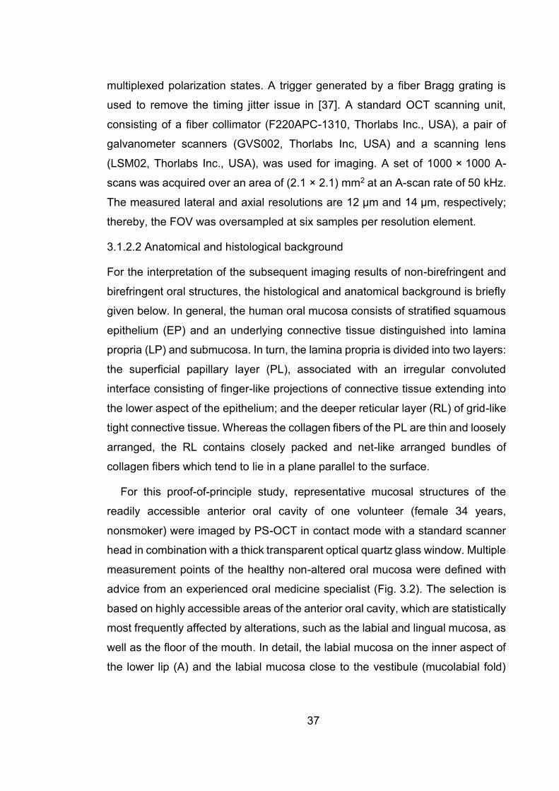
37
multiplexed polarization states. A trigger generated by a fiber Bragg grating is
used to remove the timing jitter issue in [37]. A standard OCT scanning unit,
consisting of a fiber collimator (F220APC-1310, Thorlabs Inc., USA), a pair of
galvanometer scanners (GVS002, Thorlabs Inc, USA) and a scanning lens
(LSM02, Thorlabs Inc., USA), was used for imaging. A set of 1000 × 1000 A-
scans was acquired over an area of (2.1 × 2.1) mm2 at an A-scan rate of 50 kHz.
The measured lateral and axial resolutions are 12 µm and 14 µm, respectively;
thereby, the FOV was oversampled at six samples per resolution element.
3.1.2.2 Anatomical and histological background
For the interpretation of the subsequent imaging results of non-birefringent and
birefringent oral structures, the histological and anatomical background is briefly
given below. In general, the human oral mucosa consists of stratified squamous
epithelium (EP) and an underlying connective tissue distinguished into lamina
propria (LP) and submucosa. In turn, the lamina propria is divided into two layers:
the superficial papillary layer (PL), associated with an irregular convoluted
interface consisting of finger-like projections of connective tissue extending into
the lower aspect of the epithelium; and the deeper reticular layer (RL) of grid-like
tight connective tissue. Whereas the collagen fibers of the PL are thin and loosely
arranged, the RL contains closely packed and net-like arranged bundles of
collagen fibers which tend to lie in a plane parallel to the surface.
For this proof-of-principle study, representative mucosal structures of the
readily accessible anterior oral cavity of one volunteer (female 34 years,
nonsmoker) were imaged by PS-OCT in contact mode with a standard scanner
head in combination with a thick transparent optical quartz glass window. Multiple
measurement points of the healthy non-altered oral mucosa were defined with
advice from an experienced oral medicine specialist (Fig. 3.2). The selection is
based on highly accessible areas of the anterior oral cavity, which are statistically
most frequently affected by alterations, such as the labial and lingual mucosa, as
well as the floor of the mouth. In detail, the labial mucosa on the inner aspect of
the lower lip (A) and the labial mucosa close to the vestibule (mucolabial fold)
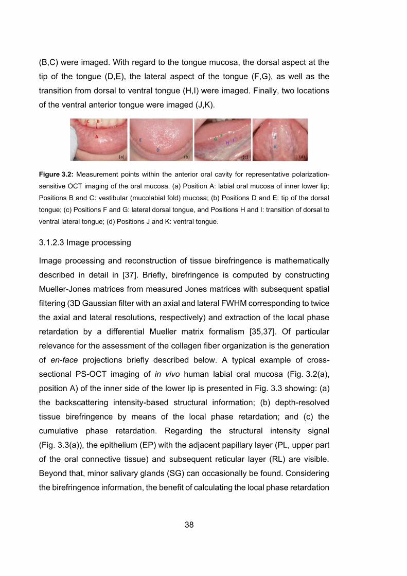
38
(B,C) were imaged. With regard to the tongue mucosa, the dorsal aspect at the
tip of the tongue (D,E), the lateral aspect of the tongue (F,G), as well as the
transition from dorsal to ventral tongue (H,I) were imaged. Finally, two locations
of the ventral anterior tongue were imaged (J,K).
Figure 3.2: Measurement points within the anterior oral cavity for representative polarization-
sensitive OCT imaging of the oral mucosa. (a) Position A: labial oral mucosa of inner lower lip;
Positions B and C: vestibular (mucolabial fold) mucosa; (b) Positions D and E: tip of the dorsal
tongue; (c) Positions F and G: lateral dorsal tongue, and Positions H and I: transition of dorsal to
ventral lateral tongue; (d) Positions J and K: ventral tongue.
3.1.2.3 Image processing
Image processing and reconstruction of tissue birefringence is mathematically
described in detail in [37]. Briefly, birefringence is computed by constructing
Mueller-Jones matrices from measured Jones matrices with subsequent spatial
filtering (3D Gaussian filter with an axial and lateral FWHM corresponding to twice
the axial and lateral resolutions, respectively) and extraction of the local phase
retardation by a differential Mueller matrix formalism [35,37]. Of particular
relevance for the assessment of the collagen fiber organization is the generation
of en-face projections briefly described below. A typical example of cross-
sectional PS-OCT imaging of in vivo human labial oral mucosa (Fig. 3.2(a),
position A) of the inner side of the lower lip is presented in Fig. 3.3 showing: (a)
the backscattering intensity-based structural information; (b) depth-resolved
tissue birefringence by means of the local phase retardation; and (c) the
cumulative phase retardation. Regarding the structural intensity signal
(Fig. 3.3(a)), the epithelium (EP) with the adjacent papillary layer (PL, upper part
of the oral connective tissue) and subsequent reticular layer (RL) are visible.
Beyond that, minor salivary glands (SG) can occasionally be found. Considering
the birefringence information, the benefit of calculating the local phase retardation
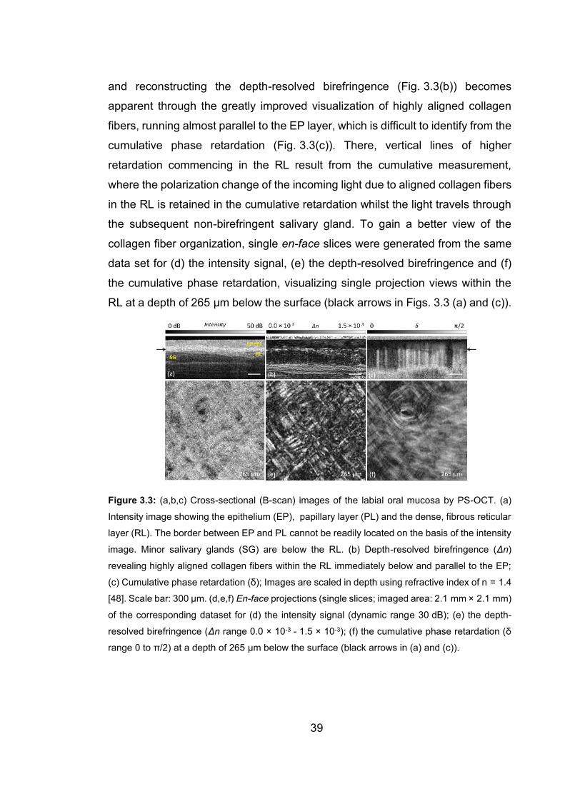
39
and reconstructing the depth-resolved birefringence (Fig. 3.3(b)) becomes
apparent through the greatly improved visualization of highly aligned collagen
fibers, running almost parallel to the EP layer, which is difficult to identify from the
cumulative phase retardation (Fig. 3.3(c)). There, vertical lines of higher
retardation commencing in the RL result from the cumulative measurement,
where the polarization change of the incoming light due to aligned collagen fibers
in the RL is retained in the cumulative retardation whilst the light travels through
the subsequent non-birefringent salivary gland. To gain a better view of the
collagen fiber organization, single en-face slices were generated from the same
data set for (d) the intensity signal, (e) the depth-resolved birefringence and (f)
the cumulative phase retardation, visualizing single projection views within the
RL at a depth of 265 µm below the surface (black arrows in Figs. 3.3 (a) and (c)).
Figure 3.3: (a,b,c) Cross-sectional (B-scan) images of the labial oral mucosa by PS-OCT. (a)
Intensity image showing the epithelium (EP), papillary layer (PL) and the dense, fibrous reticular
layer (RL). The border between EP and PL cannot be readily located on the basis of the intensity
image. Minor salivary glands (SG) are below the RL. (b) Depth-resolved birefringence (Δn)
revealing highly aligned collagen fibers within the RL immediately below and parallel to the EP;
(c) Cumulative phase retardation (δ); Images are scaled in depth using refractive index of n = 1.4
[48]. Scale bar: 300 µm. (d,e,f) En-face projections (single slices; imaged area: 2.1 mm × 2.1 mm)
of the corresponding dataset for (d) the intensity signal (dynamic range 30 dB); (e) the depth-
resolved birefringence (Δn range 0.0 × 10⁻³ - 1.5 × 10⁻³); (f) the cumulative phase retardation (δ
range 0 to π/2) at a depth of 265 µm below the surface (black arrows in (a) and (c)).
40
Even with careful inspection of the cumulative retardation (Fig. 3.3(f)), the
collagen fiber structure organization within the RL is more difficult to interpret due
to the cumulative measurement. There, the connective tissue papillae within the
overlaid PL already result in a low cumulative retardation, which is blurred across
the entire width of the en-face slices over the whole measurement depth range.
In addition to the collagen fiber layer above the salivary gland (SG), muscle
structure can be identified by the strong birefringence signal at greater depth (Fig.
3.2(b)).
Figure 3.4: (a,b) Averaged (AVG) intensity and maximum intensity projection of the depth-
resolved birefringence (MIP Δn) of N = 30 en-face slices within the RL at measurement point A in
Fig. 3.2 (a). (c) Corresponding color depth-encoded tissue birefringence (∆n) for representative
depths within the absolute range 214-367 µm below the surface. (d) Resulting color depth-
encoded birefringence using isoluminant colormap; Scaling: intensity 20 dB; tissue birefringence
Δn 0.3 × 10⁻³ - 1.5 × 10⁻³. Salivary glands marked by asterisk. The imaged area corresponds to
2.1 mm × 2.1 mm.
We anticipate that it may be beneficial in future clinical applications to visualize
the collagen organization in a single en-face projection, instead of a series of
single en-face images. Thus, we reduced the 3D stack of local birefringence ∆n
voxels to a 2D image with color-encoded depth information. This visualization is
shown for the stack of en-face slices of the preceding data set (Fig. 3.3) via the
average intensity projection (Fig. 3.4(a), AVG intensity) as well as the maximum
intensity projection of the local birefringence ∆n (Fig. 3.4(b), MIP ∆n) for the depth
range of 214-367 µm below the surface. AVG intensity gave better contrast by
inspection than MIP intensity. The depth range representing the RL is manually
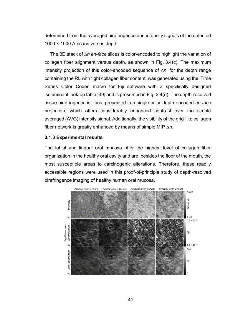
41
determined from the averaged birefringence and intensity signals of the detected
1000 × 1000 A-scans versus depth.
The 3D stack of ∆n en-face slices is color-encoded to highlight the variation of
collagen fiber alignment versus depth, as shown in Fig. 3.4(c). The maximum
intensity projection of this color-encoded sequence of ∆n, for the depth range
containing the RL with tight collagen fiber content, was generated using the ‘Time
Series Color Coder’ macro for Fiji software with a specifically designed
isoluminant look-up table [49] and is presented in Fig. 3.4(d). The depth-resolved
tissue birefringence is, thus, presented in a single color-depth-encoded en-face
projection, which offers considerably enhanced contrast over the simple
averaged (AVG) intensity signal. Additionally, the visibility of the grid-like collagen
fiber network is greatly enhanced by means of simple MIP ∆n.
3.1.3 Experimental results
The labial and lingual oral mucosa offer the highest level of collagen fiber
organization in the healthy oral cavity and are, besides the floor of the mouth, the
most susceptible areas to carcinogenic alterations. Therefore, these readily
accessible regions were used in this proof-of-principle study of depth-resolved
birefringence imaging of healthy human oral mucosa.
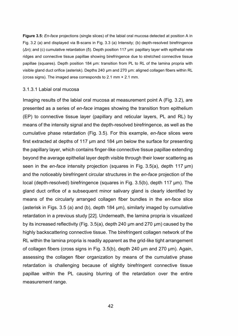
42
Figure 3.5: En-face projections (single slices) of the labial oral mucosa detected at position A in
Fig. 3.2 (a) and displayed via B-scans in Fig. 3.3 (a) Intensity; (b) depth-resolved birefringence
(Δn); and (c) cumulative retardation (δ). Depth position 117 µm: papillary layer with epithelial rete
ridges and connective tissue papillae showing birefringence due to stretched connective tissue
papillae (squares). Depth position 184 µm: transition from PL to RL of the lamina propria with
visible gland duct orifice (asterisk). Depths 240 µm and 270 µm: aligned collagen fibers within RL
(cross signs). The imaged area corresponds to 2.1 mm × 2.1 mm.
3.1.3.1 Labial oral mucosa
Imaging results of the labial oral mucosa at measurement point A (Fig. 3.2), are
presented as a series of en-face images showing the transition from epithelium
(EP) to connective tissue layer (papillary and reticular layers, PL and RL) by
means of the intensity signal and the depth-resolved birefringence, as well as the
cumulative phase retardation (Fig. 3.5). For this example, en-face slices were
first extracted at depths of 117 µm and 184 µm below the surface for presenting
the papillary layer, which contains finger-like connective tissue papillae extending
beyond the average epithelial layer depth visible through their lower scattering as
seen in the en-face intensity projection (squares in Fig. 3.5(a), depth 117 µm)
and the noticeably birefringent circular structures in the en-face projection of the
local (depth-resolved) birefringence (squares in Fig. 3.5(b), depth 117 µm). The
gland duct orifice of a subsequent minor salivary gland is clearly identified by
means of the circularly arranged collagen fiber bundles in the en-face slice
(asterisk in Figs. 3.5 (a) and (b), depth 184 µm), similarly imaged by cumulative
retardation in a previous study [22]. Underneath, the lamina propria is visualized
by its increased reflectivity (Fig. 3.5(a), depth 240 µm and 270 µm) caused by the
highly backscattering connective tissue. The birefringent collagen network of the
RL within the lamina propria is readily apparent as the grid-like tight arrangement
of collagen fibers (cross signs in Fig. 3.5(b), depth 240 µm and 270 µm). Again,
assessing the collagen fiber organization by means of the cumulative phase
retardation is challenging because of slightly birefringent connective tissue
papillae within the PL causing blurring of the retardation over the entire
measurement range.

43
Figure 3.6: (a,c) Intensity and birefringence (Δn) at different depths of the reticular layer (RL)
within the lamina propria of the inner side of the lower lip at measurement points in Fig. 3.2 (a)
labelled B (a) and C (c) presenting the vestibular mucosa (mucolabial fold) (Fig. 3.2 (a)). The
alignment of collagen fibers within the RL and around salivary glands (asterisk) are more visible
by means of the local tissue birefringence than by intensity. The imaged area corresponds to
2.1 mm × 2.1 mm. (b,d) Corresponding color depth-encoded depth-resolved birefringence. (b)
Position B: N = 33 en-face slices; Δn: 0.5 × 10⁻³ – 1.5 × 10⁻³. (d) Position C: N = 17 en-face slices;
Δn: 0.5 × 10⁻³ – 1.5 × 10⁻³.
Additionally, a series of en-face images of the labial oral mucosa at
measurement point B and C (Fig. 3.2), containing the intensity signal and the
depth-resolved birefringence, are presented below (Fig. 3.6). As expected, the
alveolar mucosa close to the vestibular fold exhibits dense fibrous connective
tissue with parallel aligned collagen fibers, which can be readily identified by the
en-face projections of the local birefringence. Furthermore, minor salivary glands
are found at larger depths presenting as low scattering regions (asterisk in
Figs. 3.6 (a) and (c)). Apart from the birefringent structure indicated by the cross
symbol in Fig. 3.6 (a), collagen fibers are highly aligned. Additionally, a capsule
of connective tissue surrounding the salivary gland is clearly visible in the depth-

44
resolved birefringence projection (asterisk in Figs. 3.6 (a) and (c)). The septae of
connective tissue originating from the capsule can be also identified (plus sign in
Fig. 3.6 (c)). Color depth-encoded en-face projections of the depth-resolved
birefringence provide single images revealing the collagen fiber organization
throughout the projected tissue depth range (Fig. 3.6 (b,d)).
3.1.3.2 Lingual oral mucosa
Malignant alterations are frequently observed at rapidly changing transitions
between different epithelial types. Therefore, the dorsal side of the volunteer’s
tongue was imaged in vivo at the tip and the outer third of the tongue body
(Fig. 3.2(b), positions D and E). The dorsal side of the tongue is covered by a
functionally masticatory mucosa with different types of lingual papillae. Images of
the distinctive specialized oral mucosa, containing mainly filiform but also
fungiform papillae, are presented for the tip of the tongue (Fig. 3.7(a), position D)
and for the lateral side of the dorsal tongue (Fig. 3.7(c), position E).
Figure 3.7: (a,c) Intensity and birefringence (Δn) at different depths of the dorsal tongue at
measurement points in Fig. 3.2(b) labelled D (a) and E (c). The birefringence of the connective
tissue core of the lingual papillae (filiform and fungiform papillae) is shown. The imaged area
corresponds to 2.1 mm × 2.1 mm. (b,d) Corresponding color depth-encoded depth-resolved
45
birefringence. (b) Position D: N = 20 en-face slices; Δn: 0.2 × 10⁻³ – 1.2 × 10⁻³. (d) Position E:
N = 30 en-face slices; Δn: 0.1 × 10⁻³ – 1.5 × 10⁻³.
In each example, a large papilla with a dominant highly reflecting connective
core containing a collagen fiber bundle can be identified, due to the non-
keratinized epithelium, as an indicator for a fungiform papillae (asterisks in Figs.
3.7(a) and (c)). In addition, smaller filiform papillae (plus signs in Fig. 3.7(c)) are
the most numerous lingual papillae with a keratin-containing epithelium and were
imaged from the side (due to the contact mode measurement) so that the
keratinized tip is not disruptive in visualizing the underlying structures. The two
small papillae at the lower right side of the en-face projections (squares in
Fig. 3.7(a)) exhibit a circular shape in combination with a backscattering signal
from larger depth but no highly reflecting connective tissue core with
corresponding birefringent signal. The reason for the weak birefringent contrast
of the border of each papilla could be due to the orientation and/or the amount of
aligned collagen fibers surrounding the papillae.
Progressing towards the posterior lateral border of the tongue (points F and G
in Fig. 3.2(c)), much smaller non-keratinized papillae become visible (asterisks in
Figs. 3.8(a) and (c)). The filiform papillae do not have a significant connective
tissue core detectable with PS-OCT but instead collagen fibers surround these
small papillae. Comparing the measurements slightly closer to the dorsal side
(position F in Fig. 3.2(c)) with those closer to the lateral tongue (position G in Fig.
3.2(c)), fewer papillae and lower birefringence due to a significantly lower content
of thick aligned collagen fibers can be noted for the more lateral position
(Fig. 3.8(c)).

46
Figure 3.8: (a,c) Intensity and birefringence (Δn) at different depths of the transition region from
dorsal to lateral tongue at measurement points in Fig. 3.2(c) labelled F (a) and G (c). The higher
birefringence of aligned collagen fibers surrounding small lingual papillae can be seen. The
imaged area corresponds to 2.1 mm × 2.1 mm. (b,d) Corresponding color depth-coded depth-
resolved birefringence. (b) Position F: N = 20 en-face slices; Δn: 0.2 × 10⁻³ – 1.5 × 10⁻³. (d)
Position G: N = 12 en-face slices; Δn: 0.1 ×10⁻³ – 1.0 × 10⁻³.
In contrast, the collagen content is increased towards the ventral tongue but
shows a high variability in fiber orientation, especially at larger depths. The parts
with no birefringence and less backscattering intensity (asterisks in Figs. 3.9(a)
and (c)) correspond to regions of the upper connective tissue (lower part of the
papillary layer) with less collagen content in comparison to the adjacent reticular
layer with highly aligned and strongly reflecting collagen fibers (cross signs in
Figs. 3.9(a) and (c)).
47
Figure 3.9: (a,c) Intensity and birefringence (Δn) at different depths of the transition from dorsal
to ventral tongue at measurement points in Fig. 3.2(c) labelled H (a) and I (c). The imaged area
corresponds to 2.1 mm × 2.1 mm. (b,d) Corresponding color depth-encoded depth-resolved
birefringence. (b) Position H: N = 21 en-face slices; Δn: 0.3 × 10⁻³ – 1.5 × 10⁻³. (d) Position I:
N = 31 en-face slices; Δn: 0.3 × 10⁻³ – 1.5 × 10⁻³.
For completeness, the ventral side of the tongue was imaged (positions J and
K in Fig. 3.2(d)). The results cannot be interpreted in a straightforward manner
on first examination. However, with the prior knowledge gained here, one can
again clearly identify less birefringent regions belonging to the upper connective
tissue (papillary layer, asterisks in Fig. 3.10(a)). Furthermore, highly reflecting
regions with lower birefringence are probably anchor points, where collagen
orientation is almost parallel to the incident sample beam, with the consequence
that only less or no birefringence is measurable (plus sign in Fig. 3.10(a)).
Additionally, the circular structures in the projection of the depth-resolved
birefringence (circles in Fig. 3.10(c)) are caused by connective tissue
surrounding a larger blood vessel. In general, the central part of the ventral

48
tongue (Fig. 3.2(d)) contains a high content of aligned collagen fibers resulting in
strong contrast in the depth-resolved birefringence projection images.
Figure 3.10: (a,c) Intensity and birefringence (Δn) at different depths of the ventral tongue at
measurement points in Fig. 3.2(d) labelled J (a) and K (c). The imaged area corresponds to
2.1 mm × 2.1 mm. (b,d) Corresponding color depth-encoded depth-resolved birefringence. (b)
Position J: N = 25 en-face slices; birefringence Δn: 0.3 × 10⁻³ – 2.5 × 10⁻³. (d) Position K: N = 16
en-face slices; Δn: 0.2 × 10⁻³ – 1.5 × 10⁻³.
3.1.4 Discussion and Conclusion
In previous PS-OCT studies, the human oral mucosa has been evaluated based
on cumulative phase retardation [20-24], which is considerably more difficult to
interpret than depth-resolved birefringence, as exemplified in Fig. 3.3 in this
manuscript [34,36]. Furthermore, we have demonstrated an approach to
collapsing 3D volumetric local-birefringence image data into depth-encoded en-
face parametric images. In particular, our results demonstrate the great potential
of depth-resolved birefringence for visualization of collagen fiber organization
within the upper connective tissue layer. In detail, the healthy reticular layer (RL)

49
we investigated, with measured thickness in the range 100-200 µm, is well suited
to be represented by a single 2D MIP image. The conditions for imaging aligned
collagen fibers within the RL of the oral lamina propria by PS-OCT are optimal
because the fiber orientation is mainly perpendicular to the incident sample
beam, particularly when using a glass plate in contact mode, as in the present
study. Further, we have shown this configuration leads to strong backscattering
signals, with good SNR, relatively large phase retardation and strong local
birefringence contrast. Even though our OCT system, with spatial resolution of
12-14 µm, cannot directly resolve the fibrillar collagen (mainly type I and III [50])
within the reticular layer, the larger fiber composite structures it forms can be
detected by the polarization-sensitive measurement with lateral oversampling (at
six samples per resolution element), which allows for the effective depiction of
the collagen fiber arrangement. Moreover, structures linked to aligned collagen
fibers, such as gland duct orifices and subsequent minor salivary glands, can be
identified. We additionally note that depth-resolved birefringence measured by
PS-OCT is sensitive to the sub-resolution, even sub-wavelength, structures not
spatially resolved, and therein lies one its key advantages as a source of
additional contrast.
En-face projections of the 3D PS-OCT data set provide new insights into the
collagen fiber organization of the oral mucosa, especially in comparison to
common PS-OCT cross-sectional (B-scan) imaging and ex vivo PSR-POL, which
is conventionally based on cross-sectioning in depth. For histological biopsy
examination of thin tissue slices by means of PSR-POL, it is challenging to
assess the collagen fiber organization as cross sections typically cut across the
collagen fiber plane. Thus, depth-resolved birefringence presented as en-face
images could provide an alternative non-invasive means to access information
on the connective tissue of the oral mucosa during prospective preoperative
examinations. At the very least, PS-OCT could serve as an adjunct to routine
histopathology for studying stromal changes at the invading front of the tumor
island, which, in turn, could help to develop a grading system for tumor
behavior/progression in vivo. For in vivo imaging, a hand-held device will be
50
necessary, with rigid or fiber-based endoscopic head [12,51,52], combined with
a sufficiently high scan rate to avoid motion artifacts. Additionally, the
combination of optical coherence angiography (OCA) [51,53] revealing
microvascular anatomy with PS-OCT may increase the potential for staging of
oral tumor invasion in advanced cancerous lesions non-invasively.
With regard to oral squamous cell carcinoma in particular, previous studies
using polarized light microscopy have shown that distinct deposits of collagen
with high birefringence, mainly around the tumor islands (neoplastic epithelial
cells/islands), are present in well-differentiated lesions [4-8,54]. The reason for
the strong birefringence could be newly formed thick bands of collagen fibers
consisting of densely packed fibrils [4,55,56]. In contrast, in moderately and
poorly differentiated squamous cell carcinoma, the collagen fibers were reticular
fibrillary and more disorganized. Thus, the extent to which invasion in oral
squamous cell carcinoma may be assessed by depth-resolved birefringence
using PS-OCT remains to be investigated in future studies. In general terms, the
motivation is the improved distinction between the tumor island and the
surrounding healthy collagen network within the thin RL and, consequently, the
better evaluation of the tumor border as a possible marker for tumor progression
in vivo. For this, the depth range used for the color-encoded MIP must be chosen
appropriately depending on the tumor dimensions and the nature of its transition
to the adjacent healthy RL.
In summary, PS-OCT with depth-resolved birefringence based on a differential
Mueller matrix formalism [35,36] was used for the first time for the visualization
of the collagen content of the fibrous connective tissue layer of healthy human
oral mucosa. In this study, we have imaged and assessed variations in collagen
fiber alignment in the human labial and lingual oral mucosa in vivo, with the main
observation of high birefringence within the lamina propria caused by a high level
of collagen organization. Looking forwards, color depth-encoded en-face
projections may offer a more intuitive way of viewing OCT data, with the aim to
make screenings of the scanned oral area more efficient. The results of this study

51
motivate future pathological and comparative studies assessing cancer-induced
stromal changes in the human oral connective tissue non-invasively by PS-OCT.
Funding
German Research Foundation (DFG WA 2812/3-1), the Australian Dental
Research Foundation, the National Institutes of Health (P41EB-015903), the
Australian Government, International Research Training Program (RTP) Fee
Offset Scholarship.
Acknowledgements
Julia Walther acknowledges receipt of financial support from the German
Research Foundation (DFG WA 2812/3-1) for the research and travel to the
University of Western Australia. Karol Karnowski, Camile S. Farah and David D.
Sampson acknowledge partial financial support of the Australian Dental
Research Foundation. Martin Villiger acknowledges support from the National
Institutes of Health (P41EB-015903). Qingyun Li acknowledges the financial
support of the Australian Government International Research Training Program
(RTP) Fee Offset Scholarship. We thank Marius Albrecht for histological advice
and Dr. Roberta Galli for useful discussions on SHG imaging. Additionally, we
thank Kota Miura for the color scale plugin for Fiji (https://imagej.net/Temporal-
Color_Code).
Disclosures
The human study was approved by the Human Research Ethics Office of the
University of Western Australia (UWA Ethics number RA/4/1/8562) with written
informed consent obtained from the participant. The authors declare that there
are no conflicts of interest related to this article.
References for Section 3.1
1. C. Rivera and B. Venegas, “Histological and molecular aspects of oral
squamous cell carcinoma (Review),” Oncol. Lett. 8(1), 7-11 (2014).
52
2. W. L. Dissanayaka, G. Pitiyage, P. V. R. Kumarasiri, R. L. P. R. Liyanage, K.
D. Dias, and W. M. Tilakaratne, “Clinical and histopathologic parameters in
survival of oral squamous cell carcinoma,” Oral Surg. Oral Med. Oral Pathol.
Oral Radiol. 113(4), 518-525 (2012).
3. L. Feller and J. Lemmer, “Oral squamous cell carcinoma: epidemiology,
clinical presentation and treatment,” J. Cancer Ther. 3(4), 263-268 (2012).
4. V. Aparna and S. Charu, “Evaluation of collagen in different grades of oral
squamous cell carcinoma by using the Picrosirius red stain - a histochemical
study,” J. Clin. Diagn. Res. 4(6), 3444-3449 (2010).
5. P. Arun Gopinathan, G. Kokila, M. Jyothi, C. Ananjan, L. Pradeep, and S. H.
Nazir, “Study of collagen birefringence in different grades of oral squamous
cell carcinoma using picrosirius red and polarized light microscopy,”
Scientifica (Cairo) 2015, 802980 (2015).
6. P. Kardam, M. Mehendiratta, S. Rehani, M. Kumra, K. Sahay, and K. Jain,
“Stromal fibers in oral squamous cell carcinoma: A possible new prognostic
indicator?,” J. Oral Maxillofac. Pathol. 20(3), 405-412 (2016).
7. R. E. John and S. Murthy, “Morphological analysis of collagen and elastic
fibers in oral squamous cell carcinoma using special stains and comparison
with Broder's and Bryne's grading systems,” Indian J. Dent. Res. 27(3), 242-
248 (2016).
8. A. Devendra, K. C. Niranjan, A. Swetha, and H. Kaveri, “Histochemical
analysis of collagen reorganization at the invasive front of oral squamous cell
carcinoma tumors,” J. Investig. Clin. Dent. 9(1), 12283 (2018).
9. C. R. Drifka, A. G. Loeffler, K. Mathewson, G. Mehta, A. Keikhosravi, Y. Liu,
S. Lemancik, W. A. Ricke, S. M. Weber, W. J. Kao, and K. W. Eliceiri,
“Comparison of picrosirius red staining with second harmonic generation
imaging for the quantification of clinically relevant collagen fiber features in
histopathology samples,” J. Histochem. Cytochem. 64(9), 519-529 (2016).
53
10. A. T. Shah and M. C. Skala, “Ex vivo label-free microscopy of head and neck
cancer patient tissues,” Proc. SPIE 9329, 93292B (2015).
11. W. S. Chen, Y. Wang, N. R. Liu, J. X. Zhang, and R. Chen, “Multiphoton
microscopic imaging of human normal and cancerous oesophagus tissue,” J.
Microsc. 253(1), 79-82 (2014).
12. J. Walther, C. Schnabel, F. Tetschke, T. Rosenauer, J. Golde, N. Ebert, M.
Baumann, C. Hannig, and E. Koch, “In vivo imaging in the oral cavity by
endoscopic optical coherence tomography,” J. Biomed. Opt. 23(7), 071207
(2018).
13. P. Wilder‐Smith, K. Lee, S. Guo, J. Zhang, K. Osann, Z. Chen, and D.
Messadi, “In vivo diagnosis of oral dysplasia and malignancy using optical
coherence tomography: Preliminary studies in 50 patients,” Lasers Surg.
Med. 41(5), 353-357 (2009).
14. P. Wilder‐Smith, W. Jung, M. Brenner, K. Osann, H. Beydoun, D. Messadi,
and Z. Chen, “In vivo optical coherence tomography for the diagnosis of oral
malignancy,” Lasers Surg. Med. 35(4), 269-275 (2004).
15. P. H. Tomlins, O. K. Adegun, E. Hagi-Pavli, K. Piper, D. Bader, and F.
Fortune, “Scattering attenuation microscopy of oral epithelial dysplasia,” J.
Biomed. Opt. 15(6), 066003 (2010).
16. M.-T. Tsai, C.-K. Lee, H.-C. Lee, H.-M. Chen, C.-P. Chiang, Y.-M. Wang, and
C.-C. Yang, “Differentiating oral lesions in different carcinogenesis stages
with optical coherence tomography,” J. Biomed. Opt. 14(4) 044028 (2009).
17. J. F. de Boer, C. K. Hitzenberger, and Y. Yasuno, “Polarization sensitive
optical coherence tomography: a review,” Biomed. Opt. Express 8(3), 1838–
1873 (2017).
18. B. Baumann, “Polarization sensitive optical coherence tomography: a review
of technology and applications,” Appl. Sci. 7(5), 474 (2017).
54
19. K. H. Kim, B. H. Park, Y. Tu, T. Hasan, B. Lee, J. Li, and J. F. de Boer,
“Polarization-sensitive optical frequency domain imaging based on
unpolarized light,” Opt. Express 19(2),552-561 (2011).
20. N. Gladkova, E. Kiseleva, N. Robakidze, I. Balalaeva, M. Karabut, E.
Gubarkova, and F. Feldchtein, “Evaluation of oral mucosa collagen condition
with cross‐polarization optical coherence tomography,” J. Biophotonics 6(4),
321-329 (2013).
21. J. Walther, J. Golde, L. Kirsten, F. Tetschke, F. Hempel, T. Rosenauer, C.
Hannig, and E. Koch, “In vivo imaging of human oral hard and soft tissues by
polarization-sensitive optical coherence tomography,” J. Biomed. Opt. 22(12),
121717 (2017).
22. Y. Yoon, W. H. Jang, P, Xiao, B. Kim, T. Wang, Q. Li, J. Y. Lee, E. Chung,
and K. H. Kim, “In vivo wide-field reflectance/fluorescence imaging and
polarization-sensitive optical coherence tomography of human oral cavity with
a forward-viewing probe,” Biomed. Opt. Express 6(2), 524-535 (2015).
23. A. M. F. Lee, L. Cahill, K. Liu, C. MacAulay, C. Poh, and P. Lane, “Wide-
field in vivo oral OCT imaging,” Biomed. Opt. Express 6(7), 2664-2674
(2015).
24. P. Sharma, Y. Verma, K. Sahu, S. Kumar, A. V. Varma, J. Kumawat, and P.
K. Gupta, “Human ex-vivo oral tissue imaging using spectral domain
polarization sensitive optical coherence tomography,” Lasers Med. Sci. 32(1),
143-150 (2017).
25. R. V. Kuranov, V. V. Sapozhnikova, I. V. Turchin, E. V. Zagainova, V. M.
Gelikonov, V. A. Kamensky, L. B. Snopova, and N. N. Prodanetz,
“Complementary use of cross-polarization and standard OCT for differential
diagnosis of pathological tissues,” Opt. Express 10(15), 707-713 (2002).
26. L. Chin, X. Yang, R. A. McLaughlin, P. B. Noble, and D. D. Sampson, “En face
parametric imaging of tissue birefringence using polarization-sensitive optical
coherence tomography,” J. Biomed. Opt. 18(6), 066005 (2013).
55
27. X. Yang, L. Chin, B. R. Klyen, T. Shavlakadze, R. A. McLaughlin, M. D.
Grounds and D. D. Sampson, “Quantitative assessment of muscle damage in
the mdx mouse model of Duchenne muscular dystrophy using polarization-
sensitive optical coherence tomography,” J. Appl. Physiol. 115(9), 1393-1401
(2013).
28. S. Makita, M. Yamanari, and Y. Yasuno, “Generalized Jones matrix optical
coherence tomography: performance and local birefringence imaging,” Opt.
Express 18(2), 854-876 (2010).
29. M. Todorovic, S. L. Jiao, and L. V. Wang, “Determination of local polarization
properties of biological samples in the presence of diattenuation by use of
Mueller optical coherence tomography,” Opt. Lett. 29(20), 2402–2404 (2004).
30. Y. Lim, M. Yamanari, S. Fukuda, Y. Kaji, T. Kiuchi, M. Miura, T. Oshika, and
Y. Yasuno, “Birefringence measurement of cornea and anterior segment by
office-based polarization-sensitive optical coherence tomography,” Biomed.
Opt. Express 2(8), 2392-2402 (2011).
31. M. J. Ju, Y.-J. Hong, S. Makita, Y. Lim, K. Kurokawa, L. Duan, M. Miura, S.
Tang, and Y. Yasuno, “Advanced multi-contrast Jones matrix optical
coherence tomography for Doppler and polarization sensitive imaging,” Opt.
Express 21(16), 19412-19436 (2013).
32. M.Yamanari, S. Tsuda, T. Kokubun, Y. Shiga, K. Omodaka, Y.Yokoyama, N.
Himori, M. Ryu, S. Kunimatsu-Sanuki, H. Takahashi, K.Maruyama, H.
Kunikata, and T. Nakazawa, “Fiber-based polarization-sensitive OCT for
birefringence imaging of the anterior eye segment,” Biomed. Opt. Express
6(2), 369-389 (2015).
33. E. Li, S. Makita, Y.-J. Hong, D. Kasaragod, and Y. Yasuno, “Three-
dimensional multi-contrast imaging of in vivo human skin by Jones matrix
optical coherence tomography,” Biomed. Opt. Express 8(3), 1290-1305
(2017).
56
34. J. Li, F. Feroldi, J. de Lange, J. M. A. Daniels, K. Grunberg and J. F. de Boer,
“Polarization sensitive optical frequency domain imaging system for
endobronchial imaging,” Optics Express 23(3), 3390–3402 (2015).
35. M. Villiger, E. Z. Zhang, S. K. Nadkarni, W.-Y. Oh, B. J. Vakoc, B. E. Bouma,
“Spectral binning for mitigation of polarization mode dispersion artifacts in
catheter-based optical frequency domain imaging,” Opt. Express 21(14),
16353–69 (2013).
36. W. C. Y. Lo, M. Villiger, A. Goldberg, G. F. Broelsch, S. Khan, C. G. Lian, W.
G. Austen Jr., M. Yurmush, and B. E. Bouma, “Longitudinal, 3D imaging of
collagen remodeling in murine hypertrophic scars in vivo using polarization-
sensitive optical frequency domain imaging,” J. Investig. Dermatol. 136(1),
84-92 (2016).
37. M. Villiger, D. Lorenser, R. A. McLaughlin, B. C. Quirk, R. W. Kirk, B. E.
Bouma, and D. D. Sampson, “Deep tissue volume imaging of birefringence
through fibre-optic needle probes for the delineation of breast tumour,” Sci.
Rep. 6, 28771 (2016).
38. M. Villiger, B. Braaf, N. Lippok, K. Otsuka, S. K. Nadkarni, and B. E. Bouma,
“Optic axis mapping with catheter-based polarization-sensitive optical
coherence tomography,” Optica 5(10), 1329-1337 (2018).
39. Q. Li, K. Karnowski, P. B. Noble, A. Cairncross, A. James, M. Villiger, and D.
D. Sampson, “Robust reconstruction of local optic axis orientation with fiber-
based polarization-sensitive optical coherence tomography,” Biomed. Opt.
Express 9(11), 5437-5455 (2018).
40. M. Villiger, K. Otsuka, A. Karanasos, P. Doradla, J. Ren, N. Lippok, M.
Shishkov, J. Daemen, R. Diletti, R. J. Van Geuns, F. Zijlstra, G. Van Soest,
P. Libby, E. Regar, S. K. Nadkarni, B. E. Bouma, “Coronary Plaque
Microstructure and Composition Modify Optical Polarization,“ JACC.
Cardiovasc. Imaging. 11(11), 1666–76 (2018).

57
41. D. Kasaragod, S. Fukuda, Y. Ueno, S. Hoshi, T. Oshika, and Y. Yasuno,
“Objective evaluation of functionality of filtering bleb based on polarization-
sensitive optical coherence tomography,” Invest. Ophthalmol. Vis. Sci. 57(4),
2305-2310 (2016).
42. F. Spöler, S. Kray, P. Grychtol, B. Hermes, J. Bornemann, M. Först, and H.
Kurz, “Simultaneous dual-band ultra-high resolution optical coherence
tomography,” Opt. Express 15(17), 10832-10842 (2007).
43. D. Sacchet, J. Moreau, P. Georges, and A. Dubois, “Simultaneous dual-band
ultra-high resolution full-field optical coherence tomography,” Opt.
Express 16(24), 19434-19446 (2008).
44. P. Cimalla, J. Walther, M. Mehner, M. Cuevas, and E. Koch, “Simultaneous
dual-band optical coherence tomography in the spectral domain for high
resolution in vivo imaging,” Opt. Express 17(22), 19486-19500 (2009).
45. Y. Lim, Y.-J. Hong, L. Duan, M. Yamanari, and Y. Yasuno, “Passive
component based multifunctional Jones matrix swept source optical
coherence tomography for Doppler and polarization imaging,” Opt. Lett.
37(11), 1958-1960 (2012).
46. B. Baumann, W. J. Choi, B. Potsaid, D. Huang, J. S. Duker, and J. G.
Fujimoto, “Swept source / Fourier domain polarization sensitive optical
coherence tomography with a passive polarization delay unit,” Opt. Express
20(9), 10229-10241 (2012).
47. Z. Wang, H.-C. Lee, O. O. Ahsen, B. K. Lee, W. J. Choi, B. Potsaid, J. Liu, V.
Jayaraman, A. Cable, M. F. Kraus, K. Liang, J. Hornegger, and J. G. Fujimoto,
“Depth-encoded all-fiber swept source polarization sensitive OCT,” Biomed.
Opt. Express 5(9), 2931-2949 (2014).
48. S. Prestin, S. I. Rotschild, C. S. Betz, and M. Kraft, “Measurement of epithelial
thickness within the oral cavity using optical coherence tomography,” Head
Neck. 34(12), 1777-1781 (2012).

58
49. J. Schindelin, I. Argand-Carreras, E. Frise, V. Kaynig, M. Longair, T. Pietzsch,
S. Preibisch, C. Rueden, S. Saalfeld, B. Schmid, J.-Y. Tinevez, D. J. White,
V. Hartenstein, K. Eliceiri, P. Tomancak, and A. Cardona, “Fiji: an open-
source platform for biological-image analysis,” Nat. Methods 9(7), 676–682,
(2012).
50. P. A. Reichart, C. W. van Wyk, J. Becker, and D. Schuppan, “Distribution of
procollagen type III, collagen type VI and tenascin in oral submucous fibrosis
(OSF),” J. Oral Pathol. Med. 23(9), 394-398 (1994).
51. M.-T. Tsai, Y. Chen, C.-Y. Lee, B.-H. Huang, N. H. Trung, Y.-J. Lee, and Y.-
L. Wang, “Noninvasive structural and microvascular anatomy of oral mucosae
using handheld optical coherence tomography,” Biomed. Opt. Express 8(11),
5001–5012 (2017).
52. J. Wang, W. Zheng, K. Lin, and Z. Huang, “Development of a hybrid Raman
spectroscopy and optical coherence tomography technique for real-time in
vivo tissue measurements,” Opt. Lett. 41(13), 3045–3048 (2016).
53. P.-H. Chen, C.-H. Wu, Y.-F. Chen, Y.C. Yeh, B.-H. Lin, K.-W. Chang, P.-Y.
Lai, M.-C. Hou, C.-L. Lu, and W. C. Kuo, “Combination of structural and
vascular optical coherence tomography for differentiating oral lesions of mice
in different carcinogenesis stages,” Biomed. Opt. Express 9(4), 1461-1476
(2018).
54. I. Sawazaki-Calone, A. Rangel, A. G. Bueno, C. F. Morais, H. M. Nagai, R. P.
Kunz, R. L. Souza, L. Rutkauskis, T. Salo, A. Almangush, and R. D. Colatta,
“The prognostic value of histopathological grading systems in oral squamous
cell carcinomas,” Oral Dis. 21(6), 755-761 (2015).
55. L. C. U. Junqueira, W. Cossermelli, and R. Brentani, “Differential staining of
collagens TypeI, II and III by Sirius red and Polarization microscopy,” Arch.
Histol. Jpn 41(3), 267-274 (1978).
59
56. G. S. Montes, R. M. Krisztan, K. M. Shigihara, R. Tokoro, P. A. Mourao, and
L. C. Junqueira, “Histochemical and morphological characterization of
reticular fibres,” Histochem. J. 65(2),131-141 (1980).
3.2 INFLUENCE OF TISSUE FIXATION ON DEPTH-
RESOLVED BIREFRINGENCE OF ORAL CAVITY TISSUE
SAMPLES
Karol Karnowski,1,2,ϯ Qingyun Li,1, ϯ Anima Poudyal,3 Martin Villiger,4 Camile S.
Farah,3,5,6 David D. Sampson1,7
Journal of Biomedical Optics (submitted)
Abstract: To advance our understanding of the contrast observed when imaging
with polarization-sensitive optical coherence tomography (PS-OCT) and its
correlation with oral cancerous pathologies, a detailed comparison with histology
provided via ex vivo fixed tissue is required. Since the effects of tissue fixation on
such polarization-based contrast measured with PS-OCT have not yet been
investigated, we performed a study on depth-resolved (i.e., local) birefringence
to assess its impact. A wide variety of ex vivo samples were measured freshly
after excision and again 24 h and 48 h after fixation. Statistically significant
1Optical + Biomedical Engineering Laboratory, Department of Electrical, Electronic & Computer
Engineering, The University of Western Australia, Perth, WA 6009, Australia
2Institute of Physical Chemistry, Polish Academy of Sciences, ul. Kasprzaka44/52, Warsaw,
Poland
3UWA Dental School, The University of Western Australia, Perth, WA 6009, Australia
4Wellman Center for Photomedicine, Harvard Medical School and Massachusetts General
Hospital, Boston, MA, USA
5Australian Centre for Oral Oncology Research and Education, Perth, WA 6009, Australia
6Oral, Maxillofacial and Dental Surgery, Fiona Stanley Hospital, Murdoch, WA 6150, Australia
7Surrey Biophotonics, School of Physics and School of Biosciences and Medicine, University of
Surrey, Guilford, Surrey GU2 7XH, United Kingdom
†These authors contributed equally.
60
changes were observed in 11 out of 12 samples; these changes represented an
increase in contrast, overall, by 11% on average. Thus, we conclude fixed
samples are suitable for studies seeking a deeper understanding of such contrast
in oral tissue pathology.
3.2.1 Introduction
Even though the potential of using optical coherence tomography (OCT) in the
oral cavity and the oropharynx has been reported in a positive light [1-3], the
evidence suggests that differentiation between healthy and potentially malignant
oral tissue is still challenging when only conventional OCT image contrast is
available. Some studies have been limited to only a few samples [2], or identified
disease from a single feature extracted from OCT scans (e.g., epithelial thickness)
[1]. In most studies reported thus far, diagnostic scores have been based on
image comparison (OCT vs. histology) by a previously trained surgeon and/or
pathologist [3-9]. The sensitivity and specificity of differentiating pathological from
normal tissue reported in those studies are in the ranges 81.5 - 93.1% and 78 -
97.3%, respectively. Detection of carcinoma in situ, squamous cell carcinoma
(SCC) versus non-cancer (sensitivity – 0.931, specificity – 0.931), or SCC versus
other pathologies (sensitivity – 0.931, specificity – 0.973) was also reported [7].
The study by Kraft et al. suggests the exact grading of dysplasia might be better
determined if microlaryngoscopy is supported by examination by OCT [10]. It is
not clear, however, what the diagnostic accuracy would be if only OCT images
were analyzed. The only study assessing the automatic classification of oral
malignancy from OCT images was performed in an animal model (hamster cheek
pouch) [11]. The performance of the sophisticated method used was failure-prone
because of common artifacts in OCT images (e.g., detector saturation due to
specular reflection).
Various extensions have been proposed to enhance the contrast in OCT
images in general. For instance, compression OCT elastography (OCE) shows
promise as a tool for interoperative assessment of cancer margins for ex vivo
human breast samples [12]. However, in vivo OCE imaging in the oral cavity with
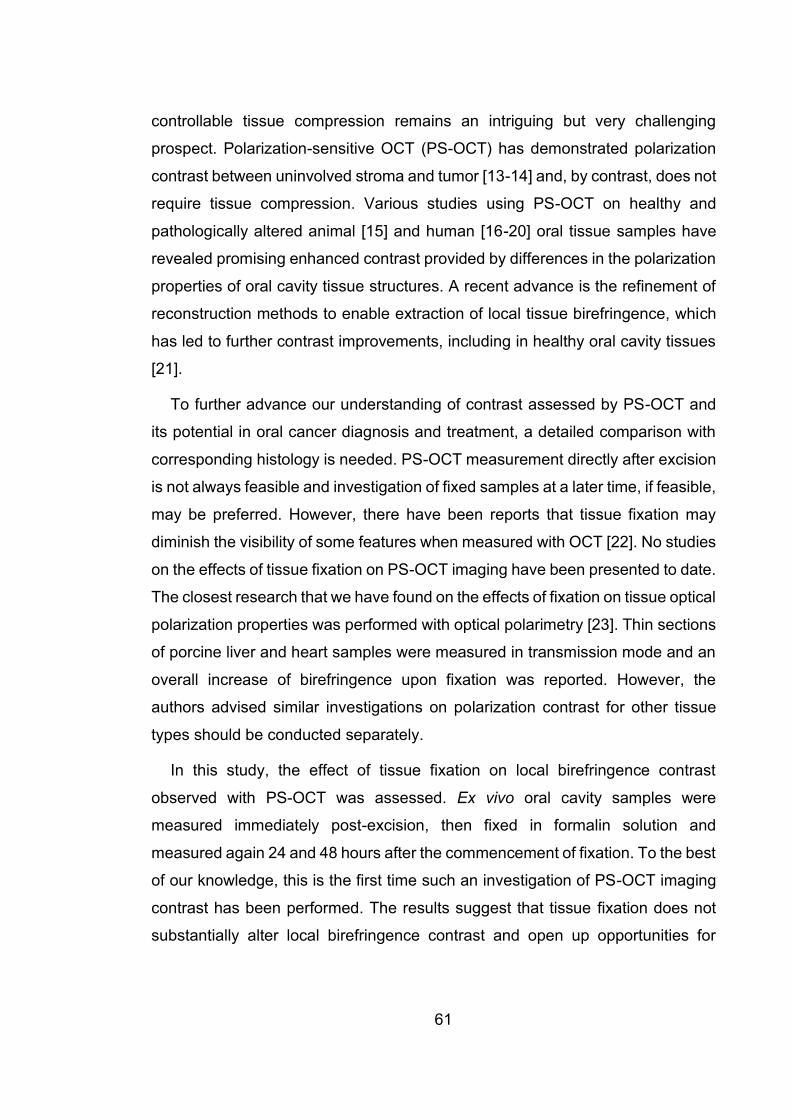
61
controllable tissue compression remains an intriguing but very challenging
prospect. Polarization-sensitive OCT (PS-OCT) has demonstrated polarization
contrast between uninvolved stroma and tumor [13-14] and, by contrast, does not
require tissue compression. Various studies using PS-OCT on healthy and
pathologically altered animal [15] and human [16-20] oral tissue samples have
revealed promising enhanced contrast provided by differences in the polarization
properties of oral cavity tissue structures. A recent advance is the refinement of
reconstruction methods to enable extraction of local tissue birefringence, which
has led to further contrast improvements, including in healthy oral cavity tissues
[21].
To further advance our understanding of contrast assessed by PS-OCT and
its potential in oral cancer diagnosis and treatment, a detailed comparison with
corresponding histology is needed. PS-OCT measurement directly after excision
is not always feasible and investigation of fixed samples at a later time, if feasible,
may be preferred. However, there have been reports that tissue fixation may
diminish the visibility of some features when measured with OCT [22]. No studies
on the effects of tissue fixation on PS-OCT imaging have been presented to date.
The closest research that we have found on the effects of fixation on tissue optical
polarization properties was performed with optical polarimetry [23]. Thin sections
of porcine liver and heart samples were measured in transmission mode and an
overall increase of birefringence upon fixation was reported. However, the
authors advised similar investigations on polarization contrast for other tissue
types should be conducted separately.
In this study, the effect of tissue fixation on local birefringence contrast
observed with PS-OCT was assessed. Ex vivo oral cavity samples were
measured immediately post-excision, then fixed in formalin solution and
measured again 24 and 48 hours after the commencement of fixation. To the best
of our knowledge, this is the first time such an investigation of PS-OCT imaging
contrast has been performed. The results suggest that tissue fixation does not
substantially alter local birefringence contrast and open up opportunities for
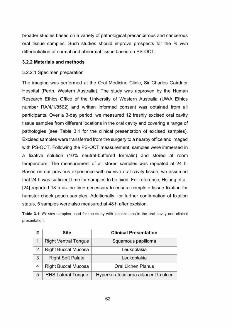
62
broader studies based on a variety of pathological precancerous and cancerous
oral tissue samples. Such studies should improve prospects for the in vivo
differentiation of normal and abnormal tissue based on PS-OCT.
3.2.2 Materials and methods
3.2.2.1 Specimen preparation
The imaging was performed at the Oral Medicine Clinic, Sir Charles Gairdner
Hospital (Perth, Western Australia). The study was approved by the Human
Research Ethics Office of the University of Western Australia (UWA Ethics
number RA/4/1/8562) and written informed consent was obtained from all
participants. Over a 3-day period, we measured 12 freshly excised oral cavity
tissue samples from different locations in the oral cavity and covering a range of
pathologies (see Table 3.1 for the clinical presentation of excised samples).
Excised samples were transferred from the surgery to a nearby office and imaged
with PS-OCT. Following the PS-OCT measurement, samples were immersed in
a fixative solution (10% neutral-buffered formalin) and stored at room
temperature. The measurement of all stored samples was repeated at 24 h.
Based on our previous experience with ex vivo oral cavity tissue, we assumed
that 24 h was sufficient time for samples to be fixed. For reference, Hsiung et al.
[24] reported 18 h as the time necessary to ensure complete tissue fixation for
hamster cheek pouch samples. Additionally, for further confirmation of fixation
status, 5 samples were also measured at 48 h after excision.
Table 3.1: Ex vivo samples used for the study with localizations in the oral cavity and clinical
presentation.
# Site Clinical Presentation
1 Right Ventral Tongue Squamous papilloma
2 Right Buccal Mucosa Leukoplakia
3 Right Soft Palate Leukoplakia
4 Right Buccal Mucosa Oral Lichen Planus
5 RHS Lateral Tongue Hyperkeratotic area adjacent to ulcer

63
6 Left Buccal Mucosa Oral Lichen Planus
7 Lower Left Lip Actinic Cheilitis
8 Left Buccal Mucosa Oral Lichen Planus
9 Left Lateral Tongue Leukoplakia
10 Left Ventral Tongue Leukoplakia
11 Right Soft Palate Leukoplakia with Pigmentation
12 Right Lower Lip Actinic Cheilitis
3.2.2.2 Polarization-sensitive OCT
Imaging was performed with a custom PS-OCT scanner developed in-house and
used previously for needle-based measurements of breast samples [13] and
adapted recently for bulk optics-based measurements [24]. The technical
specifications of the scanner are summarized as follows. The system operated
with an A-line repetition rate of 50 kHz at the center wavelength of 1310 nm and
a scanning range of 110 nm. We employed passively depth-encoded polarization
multiplexing and polarization-diverse detection to measure the full Jones matrix
containing the cumulative polarization information of backscattered light after
round-trip propagation through the sample [26]. To provide sufficient imaging
range for depth-encoded multiplexing, a custom-made sampling clock frequency-
doubling circuit was used. The resolution of the system was 13 μm and 20 μm in
tissue in the axial and lateral directions, respectively (assuming a tissue refractive
index n = 1.4 [27]). Single volumetric data sets consisting of 1000 × 1000 A-scans
covering an area of 5.1 x 5.1 mm with a depth range of 3.5 mm in air were
captured for each sample.
Data processing to extract local birefringence is summarized as follows.
Mueller-Jones matrices were constructed from the measured Jones matrices and
spatially averaged before extraction of the local birefringence using a differential
Mueller matrix algorithm [13]. An averaging kernel of 26 μm axially and 40 μm
laterally was used to improve the local birefringence contrast at the expense of a

64
two-fold reduction in spatial resolution. Both OCT intensity and local birefringence
cross-sectional images are presented in grayscale in Figs. 3.11 (a-b). Better
insight regarding the features of measured samples is provided using an en-face
slice view (Figs. 3.11c-d). The measured image data were first flattened by
automatic subtraction of the extracted position of the tissue surface, so each
projection corresponds to a given depth below the tissue surface (as marked by
the red dotted curve on the cross-sections in Figs. 3.11a-b). We note that, for
some of the samples, the surface of the excised tissue does not correspond to
the natural anatomical surface of the tissue before extraction. The flattening
procedure was introduced to create en-face projections and to enable automation
of the quantitative analysis.
Figure 3. 11: Cross-sectional (B-scan) PS-OCT images of the ex vivo right ventral tongue sample:
(a) conventional OCT intensity image, (b) depth-resolved birefringence (Δn) revealing increased
contrast compared to OCT intensity image. The en-face projections extracted from the depth
indicated by the red dotted curve for OCT intensity, (c), and birefringence, (d). Yellow dotted lines
correspond to the position of cross-sectional images. For both en-face images and birefringence
cross-sectional images, regions corresponding to low SNR, as measured in the conventional OCT
image, were masked out. Images were scaled in depth assuming a refractive index of n=1.4.

65
Surface flattening was performed and en-face slices were prepared for all
measurements. For visual presentation purposes only, the orientation angle in
the XY plane of some en-face slices was adjusted to enable the best visual
comparison between images of the same sample at different time points.
To ensure the quantitative analysis of local birefringence contrast did not suffer
from observer bias, we automated its determination. We selected data for
analysis using a binary mask (separate masks we created for each en-face depth
slice and each time point) by intensity thresholding of OCT intensity data followed
by morphological operations applied to the mask to eliminate noise and irrelevant
artifacts. The intensity-based masks were used for corresponding en-face
projections of local birefringence. All procedures, e.g., selecting the intensity
thresholding and parameters of morphological operations, were optimized on a
randomly selected data set and then applied to all data sets. The contrast was
calculated for each en-face slice starting from the surface down to a depth of
almost 800 μm, determined as the ratio of the standard deviation ( n ) to mean
value of birefringence ( )n :
nnC
n
=
, (3.1)
For samples #9 and #11 the analysis depth was reduced to 600 m and
450 m, respectively, as no sample-related signal was present below these
depths.
For each sample and time point, we performed a statistical comparison for
every en-face slice (N=112) between measurements of freshly excised samples
and fixed samples measured 24h (and 48h where available) after the
commencement of fixation. Statistical comparison first tested for normality of the
distribution using the Shapiro-Wilk test [28]. As all pairs had non-normal
distribution the Wilcoxon test [29] was used. Additionally, we analyzed the
contrast differences at given depths in the complete sample population. For every
depth slice, we calculated the contrast differences between the fresh and 24h

66
time points as well as between the fresh and 48h time points. The mean
difference and standard deviation for each slice were calculated and plotted
versus depth.
3.2.3 Results
3.2.3.1 Local birefringence qualitative contrast
Figure 3.12 shows en-face OCT intensity and local birefringence projections
extracted from different depths below the sample surface at the different time
points of the fixation process. The sample was excised from the right ventral
tongue and was pre-assessed as squamous papilloma. For this sample, we
observe high variability of birefringent structures, which most likely represent
highly aligned collagen fibers in the reticular layer, as described in our previous
study [21]. In general, in Fig. 3.12 we observe the contrast in both intensity and
birefringence due to tissue alteration induced by the fixation procedure. For the
deepest image sections (Fig. 3.12c), some examples of decreased contrast are
observed (e.g., at the location marked by the yellow asterisk). This may be the
effect of axial tissue shrinkage during fixation causing previously deeper layers
to be shifted closer to the surface. The overall and rigorous assessment of the
birefringence contrast change, however, is difficult based on a visual basis;
therefore, we undertook the quantitative analysis described above and now
present it in the following sections.
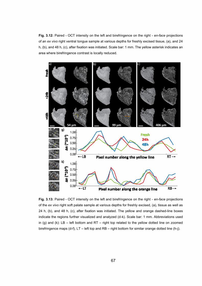
67
Fig. 3.12: Paired - OCT intensity on the left and birefringence on the right - en-face projections
of an ex vivo right ventral tongue sample at various depths for freshly excised tissue, (a), and 24
h, (b), and 48 h, (c), after fixation was initiated. Scale bar: 1 mm. The yellow asterisk indicates an
area where birefringence contrast is locally reduced.
Fig. 3.13: Paired - OCT intensity on the left and birefringence on the right - en-face projections
of the ex vivo right soft palate sample at various depths for freshly excised, (a), tissue as well as
24 h, (b), and 48 h, (c), after fixation was initiated. The yellow and orange dashed-line boxes
indicate the regions further visualized and analyzed (d-k). Scale bar: 1 mm. Abbreviations used
in (g) and (k): LB – left bottom and RT – right top related to the yellow dotted line on zoomed
birefringence maps (d-f), LT – left top and RB – right bottom for similar orange dotted line (h-j).

68
The second example (Figs. 3.13a-c) taken from the right soft palate reveals
changes in the pattern of birefringent features. Magnified views (Figs. 3.13d-j)
depict visible improvement in the birefringence contrast during the fixation
process. Two regions (yellow and orange boxes in Figs. 3.13a and b) were
selected to show the effect quantitatively. Zoomed maps of birefringence for
freshly excised (Figs. 3.13d and h), 24 h (Figs. 3.13e and i) and 48 h after fixation
was initiated (Fig. 3.13f and j), as well as plots of birefringence extracted along
selected lines (Figs. 3.13g and k), are presented.
3.2.3.2 Local birefringence quantitative contrast
To provide more than the visual assessment of the effects of tissue fixation on
polarization contrast, as described in Section 2, we applied automatic contrast
analysis for both intensity and birefringence images. The results are presented
as a boxplot (Fig. 3.14). For further statistical assessment, the paired t-test was
applied to the results. Statistically significant differences were found for all cases
except when fresh tissue was compared with 24 h after fixation for samples #1,
#2 and #9.
Fig. 3.14: Quantitative comparison of contrast change during the fixation process for all measured
samples (Fresh – green color, 24 h after fixation was initiated – red color, 48 h after fixation was
initiated – blue color). Red crosses represent outliers (values that are more than 3 times the
interquartile range away from the bottom or top of the box). Asterisks indicate statistically
significant differences in 11 out of the 12 samples.
69
To provide more insight on how the contrast changes versus depth in the
sample, we performed statistical (mean and standard deviation) slice-by-slice
assessment of the differences in contrast between freshly measured samples
and those measured 24 h or 48 h after fixation. At each sample depth, the
contrast change (24h vs. fresh and 48h vs. fresh) was calculated. Depth by depth,
we plot the mean contrast change over all samples with ribbon representing
standard deviation (Fig. 3.15). On average, we observe up to 10% increase in
mean contrast to a depth of 500 μm followed by up to 20% increase for deeper
layers. The variation, presented as a ribbon plot, is higher at deeper layers, where
the SNR is usually lower than that for preceding layers.
Fig. 3.15: Change in fixed-sample contrast versus fresh sample versus depth. Mean contrast
change over depth is presented with red-dashed curve for changes between fresh sample and
24 h after fixation, and blue-dotted curve for changes between fresh sample and 48 h after
fixation. Corresponding ribbon plots represent ± standard deviation. Solid line was added at 0%
contrast change.
3.2.4 Discussion and conclusions
In this study, the effect of fixation on polarization-sensitive contrast (local
birefringence) was investigated. Tissue samples from multiple locations in the

70
oral cavity and covering a range of pathologies were imaged with PS-OCT.
Results presented in Fig. 3.14 show that tissue fixation does not diminish the
contrast provided by the polarization-sensitive measurement; quite the contrary,
the contrast is generally increased. Statistically significant increases in contrast
were observed, compared to the contrast of fresh samples, in 11 of the 12
samples. Mean contrast change was calculated to be 11%. The greatest
increases are observed in the deepest layers, which is most likely associated with
lower SNR compared to more superficial layers. The significant differences
consistently represented an increase in birefringence contrast with fixation, which
is a positive effect considering the future utility of fixed oral cancer tissue samples.
A limitation of our work is that it does not explain the cause of the observed
changes. In the present study, however, our objective was to investigate whether
local birefringence contrast is preserved after tissue fixation, and the extent to
which fixation permits the assessment of fixed oral cavity tissues using PS-OCT.
The observed effects may be the result of tissue shrinkage, which alters the
patterns of birefringent structures in the measured samples. Such contrast
enhancement may arise from the fact that local birefringence is calculated from
the retardance 2k n z across differential depth z . In the case of axial
shrinkage, differential depth z reduces and leads to an increase in local
birefringence, other things being equal.
Promisingly, from the perspective of the utilization of fixed oral cancer tissue
samples, the enhancement of birefringent contrast, nC , removes the need to
image them immediately after excision. Furthermore, such relaxation of the need
to perform imaging in vivo facilitates the future use of recently developed
ultrahigh-resolution, extended-focus polarization-sensitive optical coherence
microscopy (PS-OCM) platform that cannot be readily moved to a dental clinic
[30]. Such a PS-OCM platform could offer detailed insight into fine sample
structure via imaging of the local optic axis, which would only be meaningful in
sample regions with sufficient local birefringence.

71
The corollary to the above arguments is the conclusions drawn by the study of
ex vivo samples will be more challenging to apply in vivo, in which images
generally show lower contrast.
In the future, the study of numerous fixed samples might lead to processing
methods, further enhancement of contrast and the emergence of clear means of
differentiation between normal and abnormal tissue. In conclusion, our results
justify the use of fixed oral tissue; however, as mentioned previously by Wood et
al. [23], we caution that similar investigations are advised if other tissue types are
to be studied.
Acknowledgments
The project was funded by the Australian Dental Research Foundation (grant no.
224-2017). K. Karnowski acknowledges support from the Polish National Agency
for Academic Exchange and the European Union’s Horizon 2020 research and
innovation program under the grant agreement no. 666295. Q. Li acknowledges
the financial support of the Australian Government International Research
Training Program (RTP) Fee Offset Scholarships. M. Villiger acknowledges
support from the National Institutes of Health (P41EB-015903).
References for Section 3.2 1. C.K. Lee et al., “Diagnosis of oral submucous fibrosis with optical coherence
tomography,” J. Biomed. Opt. 14(5), 054008 (2009).
2. N. Ozawa et al., “In vivo imaging of human labial glands using advanced
optical coherence tomography,” Oral Surg., Oral Med., Oral Pathol., Oral
Radiol., and Endod. 108(3), 425-429 (2009).
3. Z. Hamdoon, Z et al., “Optical coherence tomography in the assessment of
suspicious oral lesions: an immediate ex vivo study,” Photodiagnosis
Photodyn Ther. 10(1) 17-27 (2013).
4. O. R. Hughes et al., “Optical and molecular techniques to identify tumor
margins within the larynx,” Head Neck 32(11),1544-53 (2010).

72
5. Z. Hamdoon et al., “Structural validation of oral mucosal tissue using optical
coherence tomography,” Head Neck Oncol. 4 29 (2012).
6. W. Jerjes et al., “In vitro examination of suspicious oral lesions using optical
coherence tomography,” Br. J. Oral Maxillofac. Surg. 48(1),18-25 (2010).
7. P. Wilder-Smith et al., “In vivo diagnosis of oral dysplasia and malignancy
using optical coherence tomography: preliminary studies in 50 patients,”
Lasers Surg. Med. 41(5), 353-7 (2009).
8. Z. Hamdoon et al., “Optical coherence tomography in the assessment of oral
squamous cell carcinoma resection margins,” Photodiagnosis Photodyn.
Ther. 13, 211-7 (2016).
9. A. M. Lee et al., “Wide-field in vivo oral OCT imaging,” Biomed. Opt. Express
6(7), 2664-74 (2015).
10. M. Kraft et al., “Optical coherence tomography: significance of a new method
for assessing unclear laryngeal pathologies,” HNO 58(5), 472-9 (2010).
11. P. Pande et al., “Automated classification of optical coherence tomography
images for the diagnosis of oral malignancy in the hamster cheek pouch,” J.
Biomed. Opt. 19(8), 086022, (2014).
12. W. M. Allen et al., “Wide-field optical coherence micro-elastography for
intraoperative assessment of human breast cancer margins,” Biomed. Opt.
Express 7(10), 4139-4153 (2016).
13. M. Villiger et al., “Deep tissue volume imaging of birefringence through fibre-
optic needle probes for the delineation of breast tumour,”. Sci. Rep. 6, 28771
(2016).
14. F. A. South et al., “Differentiation of ex vivo human breast tissue using
polarization-sensitive optical coherence tomography,” Biomed. Opt. Express
5(10), 3417-3426 (2014).
15. K. H. Kim et al., “Polarization-sensitive optical frequency domain imaging
based on unpolarized light,” Opt. Express 19(2), 552–561 (2011).
73
16. N. Gladkova et al., “Evaluation of oral mucosa collagen condition with cross-
polarization optical coherence tomography,” J. Biophotonics 6(4), 321–329
(2013).
17. J. Walther et al., “In vivo imaging of human oral hard and soft tissues by
polarization-sensitive optical coherence tomography,” J. Biomed. Opt. 22(12),
121717 (2017).
18. Y. Yoon et al., “In vivo wide-field reflectance/fluorescence imaging and
polarization-sensitive optical coherence tomography of human oral cavity with
a forward-viewing probe,” Biomed. Opt. Express 6(2), 524–535 (2015).
19. P. Sharma et al., “Human ex-vivo oral tissue imaging using spectral domain
polarization sensitive optical coherence tomography,” Lasers Med. Sci. 32(1),
143–150 (2017).
20. R. Kuranov et al., “Complementary use of cross-polarization and standard
OCT for differential diagnosis of pathological tissues,” Opt. Express 10(15),
707–713 (2002).
21. J. Walther et al., “Depth-resolved birefringence imaging of collagen fiber
organization in the human oral mucosa in vivo,” Biomed. Opt. Express 10(4),
1942-1956 (2019).
22. K. Grieve et al., “Appearance of the retina with full-field optical coherence
tomography,” Invest. Ophth. Vis. Sci. 57(9), OCT96-OCT104 (2016).
23. M. Wood et al., “Effects of formalin fixation on tissue optical polarization
properties,” Phys. Med. Biol. 56 N115 (2011).
24. P. L. Hsiung, et al., “Effect of tissue preservation on imaging using ultrahigh
resolution optical coherence tomography,” J. Biomed. Opt. 10(6), 064033
(2005).
25. Q. Li et al., “Robust reconstruction of local optic axis orientation with fiber-
based polarization-sensitive optical coherence tomography," Biomed. Opt.
Express 9(11), 5437-5455 (2018).

74
26. E. Li et al., “Three-dimensional multi-contrast imaging of in vivo human skin
by Jones matrix optical coherence tomography,” Biomed. Opt. Express 8(3),
1290-1305 (2017).
27. S. Prestin et al., “Measurement of epithelial thickness within the oral cavity
using optical coherence tomography,” Head Neck 34(12), 1777-1781 (2012).
28. S. S. Shapiro, et al., “An analysis of variance test for normality (complete
samples),” Biometrika, 52(3-4), 591-611 (1965).
29. M. Hollander et al., “Nonparametric Statistical Methods,” Wiley (1973).
30. Q. Li et al., “Vectorial birefringence imaging by optical coherence microscopy
for assessing fibrillar microstructures in the cornea and limbus,” Biomed. Opt.
Express 11(2), 1122-1138 (2020).
3.3 SUMMARY
In this chapter, the advantage of local retardation is clearly demonstrated over
cumulative retardation in delineating the collagen fibres in human oral mucosa in
vivo, thanks to the fact that the local retardation directly indicates the
birefringence of a local layer in the sample, free from the cumulative effect of the
preceding layers. The capacity of studying the collagen fibre organisations non-
invasively is important, as the fibre organisations could potentially indicate health
and disease. Besides the backscattering intensity and the interesting local
retardation results demonstrated in this chapter, our PS-OCT instrument can also
provide other interesting sources of contrast that add values to the
characterisation of the sample, such as angiography and optic axis orientation,
indicating the structures of the blood vessels and underlying fibres, respectively.
In the next chapter, we demonstrate the capacity to provide these additional
valuable contrasts with our fibre-based PS-OCT.

75
4 LOCAL OPTIC AXIS IMAGING
In the previous chapter, we explored local birefringence contrast without
reference to its orientation. Here, we explore this orientation. Local optic axis
refers to the optic axis orientation of a local layer inside the sample. It was first
demonstrated with a free-space PS-OCT system, which is not as convenient as
fibre-based systems and not suitable for endoscopic applications. Yet, in SMF-
based PS-OCT systems, the optical fibres introduce unknown and wavelength-
dependent transmission matrices that sandwich the sample matrix, and hence
complicate the retrieval of local optic axis orientation. As demonstrated in Chapter
2, only the similar matrix of the local sample matrix is readily available, which
makes it challenging to extract the local optic axis. This chapter presents a robust
local optic axis algorithm in SMF-based PS-OCT with three different
configurations: standard bench-top, rotating catheter and full-range bench-top.
The smooth muscle layer in the airway was successfully segmented from its
surrounding tissue in the airway samples, both in standard bench-top and rotating
catheter configurations. Finally, multi-functional imaging capacity is presented
with PS-OCT, by incorporating angiography information derived from speckle
decorrelation, thereby, allowing the more comprehensive characterisation of the
tissue under study.
76
4.1 ROBUST RECONSTRUCTION OF LOCAL OPTIC AXIS
ORIENTATION WITH FIBER-BASED POLARIZATION-
SENSITIVE OPTICAL COHERENCE TOMOGRAPHY [54]
Qingyun Li, 1 Karol Karnowski,1 Peter B. Noble,2 Alvenia Cairncross,2 Alan
James,3 Martin Villiger4 and David D. Sampson1,5;
Biomedical Optics Express, 9(11), 5437-5455, 2018
Abstract: It is challenging to recover local optic axis orientation from samples
probed with fiber-based polarization-sensitive optical coherence tomography
(PS-OCT). In addition to the effect of preceding tissue layers, the transmission
through fiber and system elements, and imperfect system alignment need to be
compensated. Here, we present a method to retrieve the required correction
factors from measurements with depth-multiplexed PS-OCT, which accurately
measures the full Jones matrix. The correction considers both retardation and
diattenuation and is applied in the wavenumber domain, preserving the axial
resolution of the system. The robustness of the method is validated by measuring
a birefringence phantom with a misaligned system. Imaging ex-vivo lamb trachea
and human bronchus demonstrates the utility of reconstructing the local optic axis
orientation to assess smooth muscle, which is expected to be useful in the
assessment of airway smooth muscle thickness in asthma, amongst other fiber-
based applications.
1Optical+Biomedical Engineering Laboratory, Department of Electrical, Electronic & Computer
Engineering, The University of Western Australia, Perth, WA 6009, Australia
2School of Human Sciences, The University of Western Australia, Perth, WA 6009, Australia
3Department of Pulmonary Physiology and Sleep Medicine, Sir Charles Gairdner Hospital, Perth,
Australia
4Wellman Center for Photomedicine, Harvard Medical School and Massachusetts General
Hospital, Boston, MA, USA
5University of Surrey, Guildford, GU2 7XH, Surrey, United Kingdom
77
4.1.1 Introduction
Optical coherence tomography (OCT) measures the amount and path-length of
light back-scattered by tissue to reconstruct cross-sectional views of the
subsurface microstructure [1]. Many tissues feature similar scattering contrast,
which can make their differentiation difficult, and would benefit from additional
contrast. Various contrast-enhancing extensions of OCT have been proposed to
date, such as optical coherence elastography (OCE) [2, 3], OCT angiography [4,
5] and polarization-sensitive optical coherence tomography (PS-OCT) [6, 7]. PS-
OCT provides additional contrast by measuring the polarization properties of the
sample, including birefringence, degree of polarization (DOP), or optic axis
orientation. The promise of polarization imaging has been demonstrated in
various fields of medicine, including ophthalmology [8, 9], dentistry [10],
dermatology [11-13], neurology [14, 15], cardiology [16] and pulmonology [17,
18].
Cumulative birefringence (or phase retardation) and cumulative optic axis
imaging are the two most straightforward contrasts available from PS-OCT, but
since they do not directly provide local sample information, they are difficult to
interpret, especially in samples with birefringence that varies with depth. In
addition, wrapping of the cumulative phase retardation causes artifacts in
cumulative optic axis imaging [19]. It is more desirable, therefore, to assess
birefringence and optic axis orientation locally at each depth for imaging samples,
especially those composed of differently birefringent layers.
Local optic axis imaging has been demonstrated with free-space PS-OCT [20-
24]. Recently, it has also been shown that local optic axis imaging is possible with
fiber- and catheter-based PS-OCT employing non-polarization-maintaining
optical fiber [25]. This has been achieved by compensating for the transmission
through the system and fiber elements, estimated directly from the measurement
data, owing to an intrinsic symmetry constraint when measuring polarization
properties along identical illumination and detection paths [25]. The specific PS-
OCT implementation in that work used sequential illumination with two input
78
polarization states orthogonal to each other on the Poincaré sphere, and relied
on the assumption that the imaging system and the sample are free of
diattenuation. Whereas dichroism is negligible compared with birefringence in
most biological tissues, imperfect system components or inadequate alignment
can lead to readily observed diattenuation that impacts the accurate recovery of
the optic axis orientation. Further, the processing used therein employs spectral
binning and, thereby, sacrifices axial resolution to mitigate polarization mode
dispersion (PMD) present in the system components.
One of the recently investigated applications of optic axis orientation imaging
is the assessment of airway smooth muscle (ASM) structure. Thickening
(remodeling) and contraction of the ASM is considered a primary cause of
excessive narrowing and symptoms in diseases such as asthma [26], and the
capacity to clearly image the ASM could guide and improve patient therapy [27].
The idea behind imaging the optic axis orientation of the ASM relies on the
organization of the airway wall, where the ASM is oriented approximately
orthogonal to the surrounding tissue. To date, only one study on PS-OCT
measurements of ASM has been presented by Adams et al. [18], which used the
angle between the apparent optic axis orientation of the similarity transformed
local Jones matrix and a reference axis without, however, correcting for the
preceding layers. The extent to which such an assessment without depth-
correction might compromise ASM assessment in more general airway
geometries is as yet unknown.
In this manuscript, we present an improved method for local optic axis
orientation imaging that corrects for general system imperfections and maintains
the full axial resolution. It is based on a depth-multiplexed PS-OCT system that
simultaneously measures the full Jones matrix and, therefore, does not rely on
assumptions regarding the system and sample properties. The method is
insensitive to system polarization distortions, including wavelength-dependent
reference polarization states, and PMD in the system components. The full
nominal axial resolution of the employed light source remains available because
79
the corrections are directly applied in the wavenumber (k) domain. We validate
our method on tissue-like birefringence phantoms, benchmark it against the
previous reconstruction approach, and demonstrate imaging of a lamb trachea
and human bronchus ex vivo.
4.1.2 Methods
We adapted a PS-OCT system previously used for deep tissue volumetric
imaging with needle probes [28], where the needle probes were replaced with a
standard scanning microscope configuration. The light source used is a
wavelength-swept laser (Axsun Technologies, Bellerica, MA, USA), centered at
1310 nm, with a full sweep range of 100 nm at a 50 kHz sweep rate. 1% of the
power of the source, split by a fiber coupler, was directed to a fiber Bragg grating
and reflection from the grating was employed to trigger the acquisition and
minimize timing jitter. The remaining power of the source, further split by a fiber
coupler, was delivered to the sample (80%) and reference (20%) arms via
conventional single-mode fibers, respectively. The sampling clock generated by
the laser was electronically frequency-doubled to extend the total depth range
from 5.0 mm to 10.0 mm. The increased imaging range enabled depth-encoded
polarization multiplexing by passively delaying one of two orthogonal polarization
states illuminating the sample with a free-space-based polarization delay unit
(PDU) [29, 30]. An optical circulator delivered the light from the PDU to a standard
scanning microscope configuration, which contains a fiber collimator (F220APC-
1310, Thorlabs Inc., New Jersey, USA), a galvanometric x-y scanner (GVS002,
Thorlabs Inc.) and a scan lens (LSM03, Thorlabs Inc.), providing approximately
25 μm lateral resolution. For lateral scanning, the distance between adjacent A-
lines was adjusted to 5 μm for slight oversampling. In the reference arm, a fiber
coupler was used to direct the light to the reference mirror and on to the receiver,
imparting a 6 dB loss but avoiding potential polarization effects that could be
caused by a circulator. The sample signal and reference signal were combined
with a commercial polarization-diverse optical mixer (PDOM-1310, Finisar,
Sunnyvale, USA) and detected with a pair of balanced detectors (PDB460C-AC,
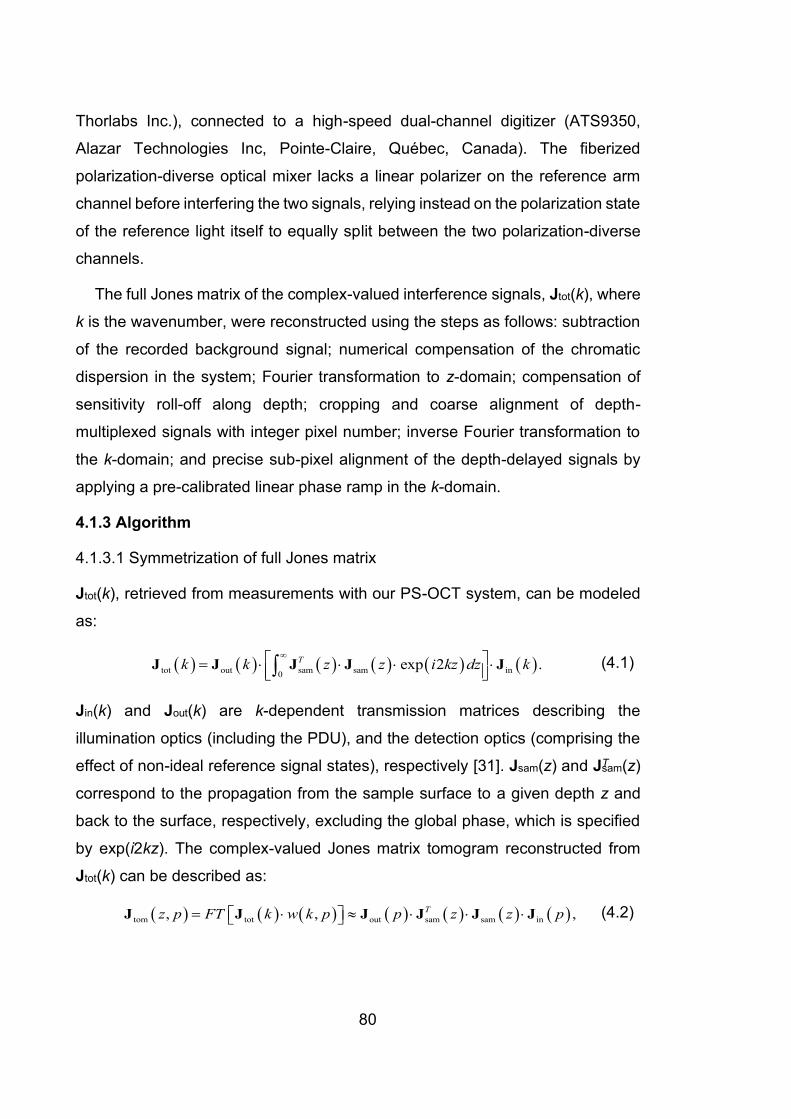
80
Thorlabs Inc.), connected to a high-speed dual-channel digitizer (ATS9350,
Alazar Technologies Inc, Pointe-Claire, Québec, Canada). The fiberized
polarization-diverse optical mixer lacks a linear polarizer on the reference arm
channel before interfering the two signals, relying instead on the polarization state
of the reference light itself to equally split between the two polarization-diverse
channels.
The full Jones matrix of the complex-valued interference signals, Jtot(k), where
k is the wavenumber, were reconstructed using the steps as follows: subtraction
of the recorded background signal; numerical compensation of the chromatic
dispersion in the system; Fourier transformation to z-domain; compensation of
sensitivity roll-off along depth; cropping and coarse alignment of depth-
multiplexed signals with integer pixel number; inverse Fourier transformation to
the k-domain; and precise sub-pixel alignment of the depth-delayed signals by
applying a pre-calibrated linear phase ramp in the k-domain.
4.1.3 Algorithm
4.1.3.1 Symmetrization of full Jones matrix
Jtot(k), retrieved from measurements with our PS-OCT system, can be modeled
as:
( ) ( ) ( ) ( ) ( ) ( )tot out sam sam in0
exp 2 .Tk k z z i kz dz k =
J J J J J (4.1)
Jin(k) and Jout(k) are k-dependent transmission matrices describing the
illumination optics (including the PDU), and the detection optics (comprising the
effect of non-ideal reference signal states), respectively [31]. Jsam(z) and JTsam(z)
correspond to the propagation from the sample surface to a given depth z and
back to the surface, respectively, excluding the global phase, which is specified
by exp(i2kz). The complex-valued Jones matrix tomogram reconstructed from
Jtot(k) can be described as:
( ) ( ) ( ) ( ) ( ) ( ) ( )tom tot out sam sam in, , ,Tz p FT k w k p p z z p= J J J J J J (4.2)
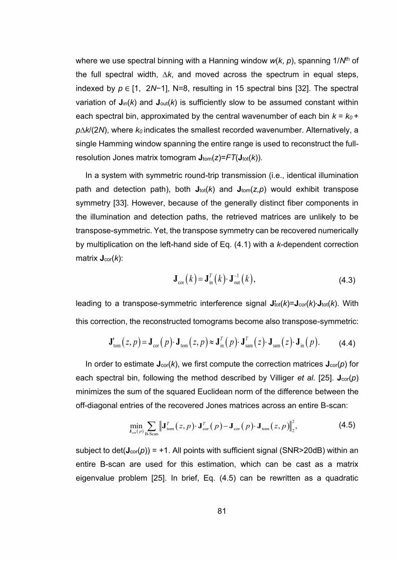
81
where we use spectral binning with a Hanning window w(k, p), spanning 1/Nth of
the full spectral width, ∆k, and moved across the spectrum in equal steps,
indexed by p ∈ [1, 2N−1], N=8, resulting in 15 spectral bins [32]. The spectral
variation of Jin(k) and Jout(k) is sufficiently slow to be assumed constant within
each spectral bin, approximated by the central wavenumber of each bin k = k0 +
p∆k/(2N), where k0 indicates the smallest recorded wavenumber. Alternatively, a
single Hamming window spanning the entire range is used to reconstruct the full-
resolution Jones matrix tomogram Jtom(z)=FT(Jtot(k)).
In a system with symmetric round-trip transmission (i.e., identical illumination
path and detection path), both Jtot(k) and Jtom(z,p) would exhibit transpose
symmetry [33]. However, because of the generally distinct fiber components in
the illumination and detection paths, the retrieved matrices are unlikely to be
transpose-symmetric. Yet, the transpose symmetry can be recovered numerically
by multiplication on the left-hand side of Eq. (4.1) with a k-dependent correction
matrix Jcor(k):
( ) ( ) ( )1
cor in out ,Tk k k−= J J J (4.3)
leading to a transpose-symmetric interference signal J′tot(k)=Jcor(k)‧Jtot(k). With
this correction, the reconstructed tomograms become also transpose-symmetric:
( ) ( ) ( ) ( ) ( ) ( ) ( )tom cor tom in sam sam in, , .T Tz p p z p p z z p = J J J J J J J (4.4)
In order to estimate Jcor(k), we first compute the correction matrices Jcor(p) for
each spectral bin, following the method described by Villiger et al. [25]. Jcor(p)
minimizes the sum of the squared Euclidean norm of the difference between the
off-diagonal entries of the recovered Jones matrices across an entire B-scan:
( )( ) ( ) ( ) ( )
cor
2
tom cor cor tom 2B-Scan
min , , ,T T
pz p p p z p −
JJ J J J (4.5)
subject to det(Jcor(p)) = +1. All points with sufficient signal (SNR>20dB) within an
entire B-scan are used for this estimation, which can be cast as a matrix
eigenvalue problem [25]. In brief, Eq. (4.5) can be rewritten as a quadratic
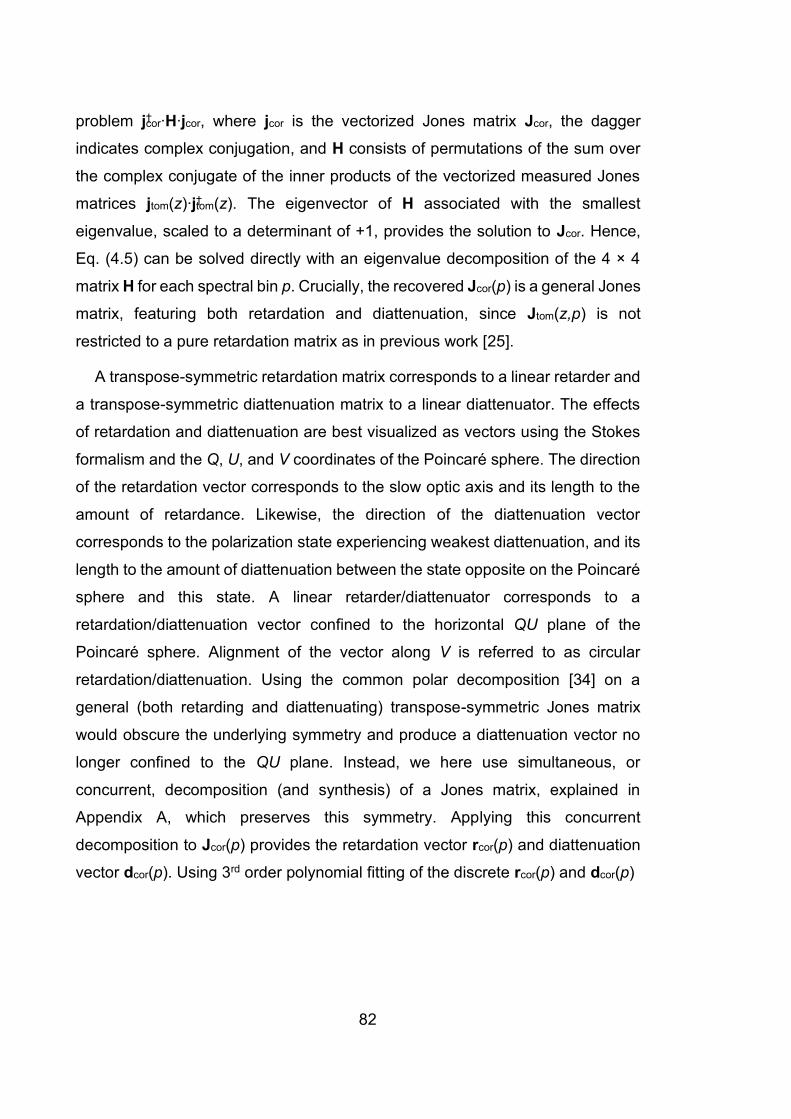
82
problem j†cor∙H∙jcor, where jcor is the vectorized Jones matrix Jcor, the dagger
indicates complex conjugation, and H consists of permutations of the sum over
the complex conjugate of the inner products of the vectorized measured Jones
matrices jtom(z)∙j†tom(z). The eigenvector of H associated with the smallest
eigenvalue, scaled to a determinant of +1, provides the solution to Jcor. Hence,
Eq. (4.5) can be solved directly with an eigenvalue decomposition of the 4 × 4
matrix H for each spectral bin p. Crucially, the recovered Jcor(p) is a general Jones
matrix, featuring both retardation and diattenuation, since Jtom(z,p) is not
restricted to a pure retardation matrix as in previous work [25].
A transpose-symmetric retardation matrix corresponds to a linear retarder and
a transpose-symmetric diattenuation matrix to a linear diattenuator. The effects
of retardation and diattenuation are best visualized as vectors using the Stokes
formalism and the Q, U, and V coordinates of the Poincaré sphere. The direction
of the retardation vector corresponds to the slow optic axis and its length to the
amount of retardance. Likewise, the direction of the diattenuation vector
corresponds to the polarization state experiencing weakest diattenuation, and its
length to the amount of diattenuation between the state opposite on the Poincaré
sphere and this state. A linear retarder/diattenuator corresponds to a
retardation/diattenuation vector confined to the horizontal QU plane of the
Poincaré sphere. Alignment of the vector along V is referred to as circular
retardation/diattenuation. Using the common polar decomposition [34] on a
general (both retarding and diattenuating) transpose-symmetric Jones matrix
would obscure the underlying symmetry and produce a diattenuation vector no
longer confined to the QU plane. Instead, we here use simultaneous, or
concurrent, decomposition (and synthesis) of a Jones matrix, explained in
Appendix A, which preserves this symmetry. Applying this concurrent
decomposition to Jcor(p) provides the retardation vector rcor(p) and diattenuation
vector dcor(p). Using 3rd order polynomial fitting of the discrete rcor(p) and dcor(p)

83
Figure 4.1: Example of symmetrization of full Jones matrix with an ex-vivo lamb trachea sample.
(a) Cross-sectional intensity image of the sample. M: Mucosa; ASM: Airway smooth muscle; C:
Cartilage. (b) Plots of retardation vectors rcor(p) (circles) and diattenuation vectors dcor(p) (stars)
of Jcor(p) and their 3rd order polynomial fits rcor(k) (solid lines) and dcor(k) (dashed lines) across
the full spectrum. kc is the central wavenumber. Normalized histogram of the circular (V)
component of the retardation vectors (c) and diattenuation vectors (d) of the full Jones matrix
before (red, Jtom(z)) and after (blue, J′tom(z)) symmetrization. Images of the retardation vectors of
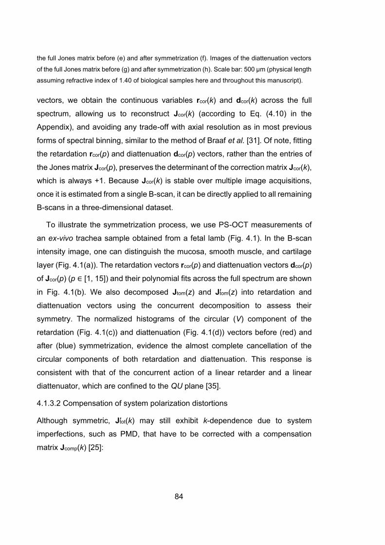
84
the full Jones matrix before (e) and after symmetrization (f). Images of the diattenuation vectors
of the full Jones matrix before (g) and after symmetrization (h). Scale bar: 500 μm (physical length
assuming refractive index of 1.40 of biological samples here and throughout this manuscript).
vectors, we obtain the continuous variables rcor(k) and dcor(k) across the full
spectrum, allowing us to reconstruct Jcor(k) (according to Eq. (4.10) in the
Appendix), and avoiding any trade-off with axial resolution as in most previous
forms of spectral binning, similar to the method of Braaf et al. [31]. Of note, fitting
the retardation rcor(p) and diattenuation dcor(p) vectors, rather than the entries of
the Jones matrix Jcor(p), preserves the determinant of the correction matrix Jcor(k),
which is always +1. Because Jcor(k) is stable over multiple image acquisitions,
once it is estimated from a single B-scan, it can be directly applied to all remaining
B-scans in a three-dimensional dataset.
To illustrate the symmetrization process, we use PS-OCT measurements of
an ex-vivo trachea sample obtained from a fetal lamb (Fig. 4.1). In the B-scan
intensity image, one can distinguish the mucosa, smooth muscle, and cartilage
layer (Fig. 4.1(a)). The retardation vectors rcor(p) and diattenuation vectors dcor(p)
of Jcor(p) (p ∈ [1, 15]) and their polynomial fits across the full spectrum are shown
in Fig. 4.1(b). We also decomposed Jtom(z) and J′tom(z) into retardation and
diattenuation vectors using the concurrent decomposition to assess their
symmetry. The normalized histograms of the circular (V) component of the
retardation (Fig. 4.1(c)) and diattenuation (Fig. 4.1(d)) vectors before (red) and
after (blue) symmetrization, evidence the almost complete cancellation of the
circular components of both retardation and diattenuation. This response is
consistent with that of the concurrent action of a linear retarder and a linear
diattenuator, which are confined to the QU plane [35].
4.1.3.2 Compensation of system polarization distortions
Although symmetric, J′tot(k) may still exhibit k-dependence due to system
imperfections, such as PMD, that have to be corrected with a compensation
matrix Jcomp(k) [25]:
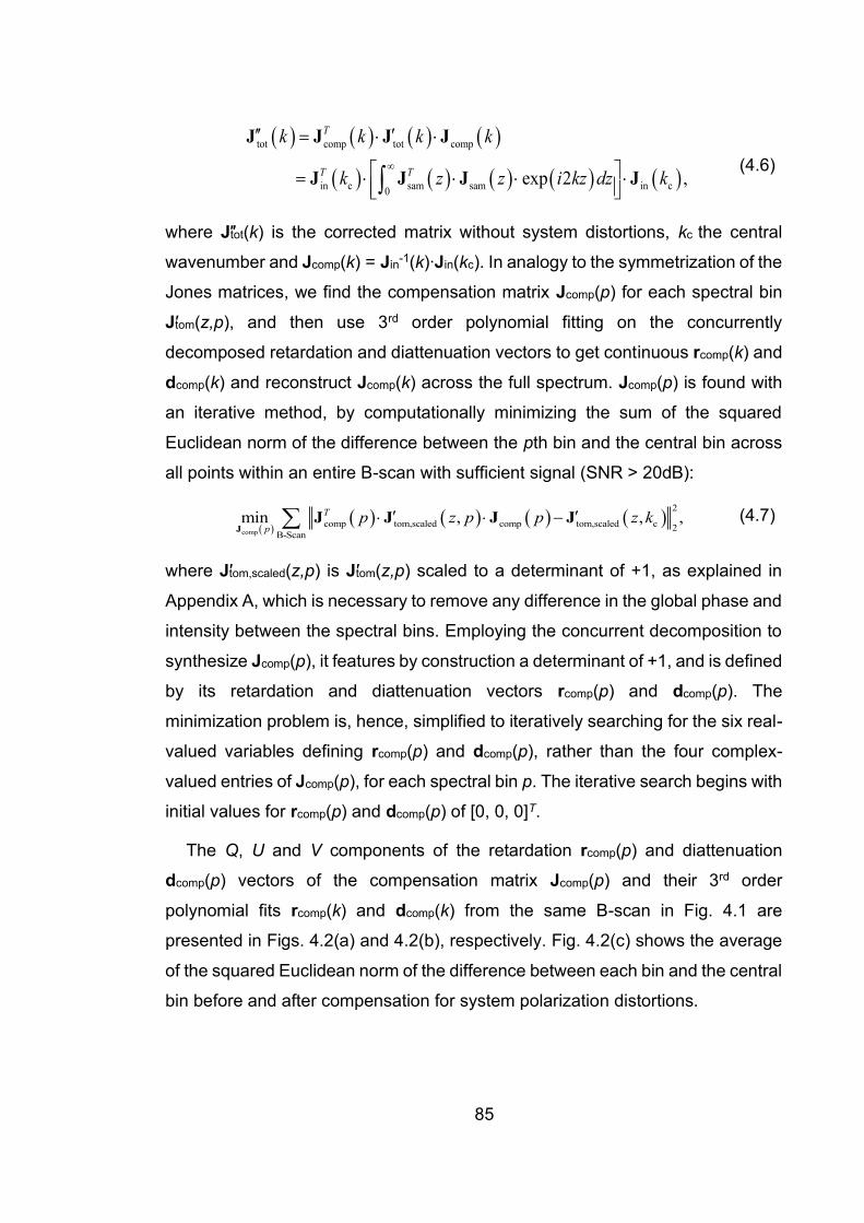
85
( ) ( ) ( ) ( )
( ) ( ) ( ) ( ) ( )
tot comp tot comp
in c sam sam in c0
exp 2 ,
T
T T
k k k k
k z z i kz dz k
=
=
J J J J
J J J J (4.6)
where J″tot(k) is the corrected matrix without system distortions, kc the central
wavenumber and Jcomp(k) = Jin-1(k)∙Jin(kc). In analogy to the symmetrization of the
Jones matrices, we find the compensation matrix Jcomp(p) for each spectral bin
J′tom(z,p), and then use 3rd order polynomial fitting on the concurrently
decomposed retardation and diattenuation vectors to get continuous rcomp(k) and
dcomp(k) and reconstruct Jcomp(k) across the full spectrum. Jcomp(p) is found with
an iterative method, by computationally minimizing the sum of the squared
Euclidean norm of the difference between the pth bin and the central bin across
all points within an entire B-scan with sufficient signal (SNR > 20dB):
( )( ) ( ) ( ) ( )
comp
2
comp tom,scaled comp tom,scaled c 2B-Scan
min , , ,T
pp z p p z k −
JJ J J J (4.7)
where J′tom,scaled(z,p) is J′tom(z,p) scaled to a determinant of +1, as explained in
Appendix A, which is necessary to remove any difference in the global phase and
intensity between the spectral bins. Employing the concurrent decomposition to
synthesize Jcomp(p), it features by construction a determinant of +1, and is defined
by its retardation and diattenuation vectors rcomp(p) and dcomp(p). The
minimization problem is, hence, simplified to iteratively searching for the six real-
valued variables defining rcomp(p) and dcomp(p), rather than the four complex-
valued entries of Jcomp(p), for each spectral bin p. The iterative search begins with
initial values for rcomp(p) and dcomp(p) of [0, 0, 0]T.
The Q, U and V components of the retardation rcomp(p) and diattenuation
dcomp(p) vectors of the compensation matrix Jcomp(p) and their 3rd order
polynomial fits rcomp(k) and dcomp(k) from the same B-scan in Fig. 4.1 are
presented in Figs. 4.2(a) and 4.2(b), respectively. Fig. 4.2(c) shows the average
of the squared Euclidean norm of the difference between each bin and the central
bin before and after compensation for system polarization distortions.
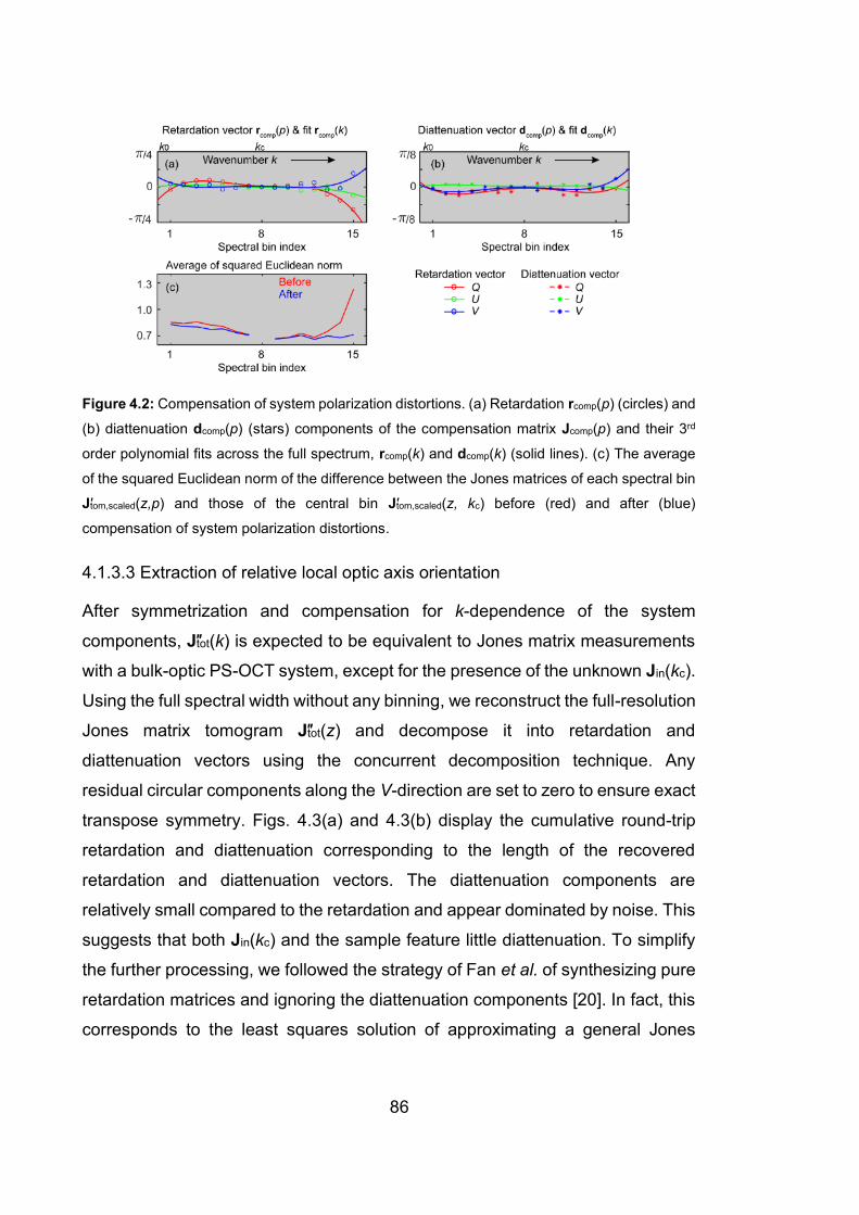
86
Figure 4.2: Compensation of system polarization distortions. (a) Retardation rcomp(p) (circles) and
(b) diattenuation dcomp(p) (stars) components of the compensation matrix Jcomp(p) and their 3rd
order polynomial fits across the full spectrum, rcomp(k) and dcomp(k) (solid lines). (c) The average
of the squared Euclidean norm of the difference between the Jones matrices of each spectral bin
J′tom,scaled(z,p) and those of the central bin J′tom,scaled(z, kc) before (red) and after (blue)
compensation of system polarization distortions.
4.1.3.3 Extraction of relative local optic axis orientation
After symmetrization and compensation for k-dependence of the system
components, J″tot(k) is expected to be equivalent to Jones matrix measurements
with a bulk-optic PS-OCT system, except for the presence of the unknown Jin(kc).
Using the full spectral width without any binning, we reconstruct the full-resolution
Jones matrix tomogram J″tot(z) and decompose it into retardation and
diattenuation vectors using the concurrent decomposition technique. Any
residual circular components along the V-direction are set to zero to ensure exact
transpose symmetry. Figs. 4.3(a) and 4.3(b) display the cumulative round-trip
retardation and diattenuation corresponding to the length of the recovered
retardation and diattenuation vectors. The diattenuation components are
relatively small compared to the retardation and appear dominated by noise. This
suggests that both Jin(kc) and the sample feature little diattenuation. To simplify
the further processing, we followed the strategy of Fan et al. of synthesizing pure
retardation matrices and ignoring the diattenuation components [20]. In fact, this
corresponds to the least squares solution of approximating a general Jones

87
matrix with a pure retardation matrix. But rather than using SU(2) Jones matrices,
we construct SO(3) rotation matrices from the retardation vectors [36] to enable
effective incoherent spatial averaging, similar to the averaging of Mueller
matrices [28]. Moreover, conversion to SO(3) removes the sign ambiguity of the
retardation vector in J″tot(z). To suppress speckle, the SO(3) matrices are
weighted with the tomogram intensity signal (the magnitude of the determinant of
the Jones matrix J″tot(z) before scaling [37]) and then spatially averaged by a
three-dimensional Gaussian kernel (FWHM approximately twice the speckle
width in both lateral and axial directions), using the same formulation and
computationally efficient implementation of the Euclidean mean described
previously [25]. In short, the averaged rotation matrices contain depolarization
components that have to be removed in order to remain in SO(3). We used three-
dimensional averaging throughout this work, but two-dimensional filtering may be
necessary for in vivo imaging and the presence of motion artifacts. The effect on
the retardance of spatially filtered SO(3) rotation matrices is shown in Fig. 4.3(c).
In addition, retardance from the central A-lines of the yellow and green boxes
before (Fig. 4.3(a)) and after (Fig. 4.3(c)) spatial filtering are plotted in Figs. 4.3(d)
and 3(e), respectively.
Figure 4.3: Generation and spatial filtering of cumulative SO(3). Image of cumulative retardance
(a) and (b) diattenuation of the sample decomposed from the general Jones matrix. (c) Image of
retardance of SO(3) after spatial averaging. (d) Retardance of the central A-line in the yellow box
in (a) before (red) and in (b) after spatial averaging (blue). (e) Retardance of the central A-line in
the green box in (a) before (red) and in (b) after spatial averaging (blue).
88
The recovered SO(3) retardation matrices after spatial filtering, denoted as
Rrt(z), express the retardation accumulated during the round trip to depth z and
back. If Rst(z) is the single trip retardation matrix to depth z, we have Rrt(z) = D∙
RTst (z)∙D∙Rst(z), where D is a diagonal matrix diag(1, 1, −1). In SO(3), D∙MT∙D
corresponds to the reverse transmission through element M, in analogy to the
simple transpose of Jones matrices [33]. Rst(z) can be described as the
sequential transmission through individual tissue layers Qn of thickness dz, the
axial sampling distance:
( )st n 2 1 0.n dz = R Q Q Q Q (4.8)
Each layer is assumed to act as a linear retarder. Its retardation vector defines
the local retardation and local optic axis orientation that we are attempting to
recover. The sequence of linear retarders defining Rst(z) results in a general
retarder. However, we only measure the round-trip matrix Rrt(z), which cancels
the circular retardation component. Hence, we follow the recursive reconstruction
of Fan et al. [20] to isolate the round-trip transmission through each individual
layer and compute its square root to recover the single-pass transmission and
construct Rst(z) for the subsequent layer, starting at z = 0:
( )
( )
( )
( ) ( ) ( )
0 rt
1 0 rt 0
2 1 0 rt 0 1
n st rt st
0
2
1 1 ,
T
T T
T
dz
dz
n dz n dz n dz
=
=
=
= − −
Q R
Q D Q D R Q
Q D Q Q D R Q Q
Q D R D R R
(4.9)
where we used the fact that MT = M−1 in SO(3). At pixel locations with insufficient
signal (SNR < 5dB), Q is replaced with the identity matrix. Finally, the retardation
vector of Q is retrieved and axially filtered with a rectangular filter equal in width
to the axial FWHM of the spatial filter previously used to average the SO(3)
retardation matrices. The length and orientation of this filtered vector provide the
local retardation and the local optic axis orientation, respectively.

89
Although we confirmed that Jin(kc) is minimally diattenuating, its retardation
component still impacts Rrt(z) and defines Rrt(z = 0). Taking its matrix root to
compute Q0 only recovers the linear retardation of Jin(kc). The non-detectable
circular retarding component in Jin(kc) offsets the recovered optic axis
orientations of the sample, making the optic axis measurement relative.
4.1.4 Results
4.1.4.1 Validation with birefringence phantoms
We validated the method using a custom-made birefringence phantom (Sample
#1). We cut thin strips from a polylactic acid (PLA) 3D printer filament. The PLA
filament exhibits intrinsic birefringence with its fast optic axis parallel to the
filament’s axis [38]. The strips were prepared so the longer edge is parallel to the
optic axis of the filament. We arranged multiple thin strips at different angles with
respect to the laboratory frame and used adhesive tape to fix the assembly. No
contrast between strips is visible for the OCT intensity, local phase retardation,
and depolarization index images (Figs. 4.4(a-c)), where the depolarization index
was computed following Lippok et al. [39]. The local optic axis visualization,
however, strongly correlates with the orientation of each strip (Fig. 4.4(d)). Note
that since the measured optic axis orientation is relative to an unknown laboratory
frame, an offset angle is manually applied here to the measured optic axis
orientation to align it with the optic axis wheel, purely for ease of comparison.
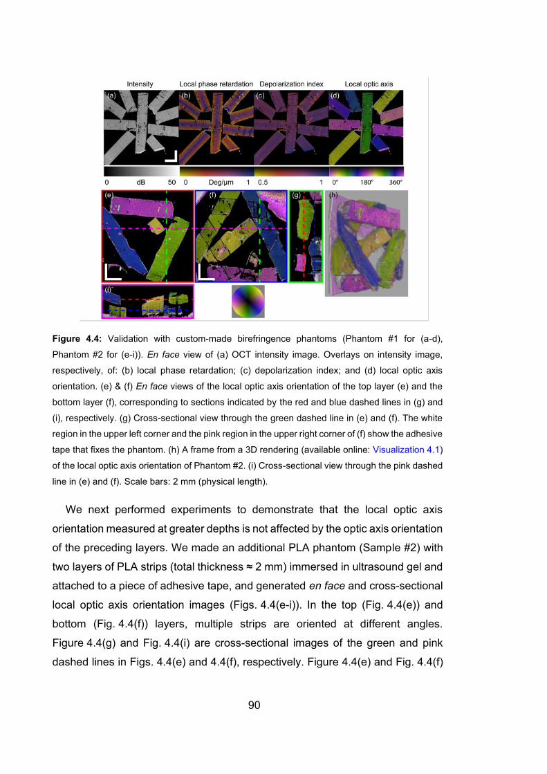
90
Figure 4.4: Validation with custom-made birefringence phantoms (Phantom #1 for (a-d),
Phantom #2 for (e-i)). En face view of (a) OCT intensity image. Overlays on intensity image,
respectively, of: (b) local phase retardation; (c) depolarization index; and (d) local optic axis
orientation. (e) & (f) En face views of the local optic axis orientation of the top layer (e) and the
bottom layer (f), corresponding to sections indicated by the red and blue dashed lines in (g) and
(i), respectively. (g) Cross-sectional view through the green dashed line in (e) and (f). The white
region in the upper left corner and the pink region in the upper right corner of (f) show the adhesive
tape that fixes the phantom. (h) A frame from a 3D rendering (available online: Visualization 4.1)
of the local optic axis orientation of Phantom #2. (i) Cross-sectional view through the pink dashed
line in (e) and (f). Scale bars: 2 mm (physical length).
We next performed experiments to demonstrate that the local optic axis
orientation measured at greater depths is not affected by the optic axis orientation
of the preceding layers. We made an additional PLA phantom (Sample #2) with
two layers of PLA strips (total thickness ≈ 2 mm) immersed in ultrasound gel and
attached to a piece of adhesive tape, and generated en face and cross-sectional
local optic axis orientation images (Figs. 4.4(e-i)). In the top (Fig. 4.4(e)) and
bottom (Fig. 4.4(f)) layers, multiple strips are oriented at different angles.
Figure 4.4(g) and Fig. 4.4(i) are cross-sectional images of the green and pink
dashed lines in Figs. 4.4(e) and 4.4(f), respectively. Figure 4.4(e) and Fig. 4.4(f)
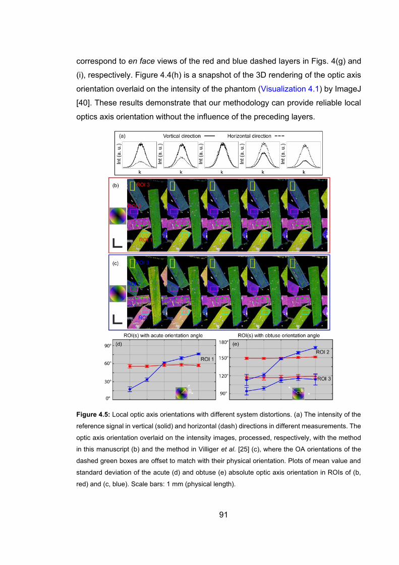
91
correspond to en face views of the red and blue dashed layers in Figs. 4(g) and
(i), respectively. Figure 4.4(h) is a snapshot of the 3D rendering of the optic axis
orientation overlaid on the intensity of the phantom (Visualization 4.1) by ImageJ
[40]. These results demonstrate that our methodology can provide reliable local
optics axis orientation without the influence of the preceding layers.
Figure 4.5: Local optic axis orientations with different system distortions. (a) The intensity of the
reference signal in vertical (solid) and horizontal (dash) directions in different measurements. The
optic axis orientation overlaid on the intensity images, processed, respectively, with the method
in this manuscript (b) and the method in Villiger et al. [25] (c), where the OA orientations of the
dashed green boxes are offset to match with their physical orientation. Plots of mean value and
standard deviation of the acute (d) and obtuse (e) absolute optic axis orientation in ROIs of (b,
red) and (c, blue). Scale bars: 1 mm (physical length).
92
We next show here that, through symmetrization and compensation of system
PMD, our method becomes robust to variations in the system. We do this by
deliberately introducing distortions into the system. We repeatedly measured the
same PLA phantom (Figs. 4.5(b-e)), whilst varying the distortions in between
measurements by adjusting the polarization controller in the reference arm
(Fig. 4.5(a)). Because the polarization mixer lacks a linear polarizer on the
reference input, varying the reference polarization state is akin to introducing
system diattenuation [31]. To characterize the distortion, we analyzed the
intensity in each reference polarization state by summing the square of the
magnitude of the demodulated complex-valued fringe signals (dominated by the
reference signal) over the two input states. The optic axis orientations remain
almost unchanged regardless of the distortions (Fig. 4.5(b)). In addition, a
benchmark against the method published by Villiger et al. [25] is also performed,
the results of which (Fig. 4.5(c)) are expected to be suboptimal due to its neglect
of system diattenuation. Briefly, in Villiger et al. [25], the imaging system uses two
sequential probing Stokes vectors orthogonal to each other on the Poincaré
sphere, and the processing assumes pure retardation of the sample and the
system. To ease the comparison with a common reference, the measured relative
optic axis orientations in Figs. 4.5(b) and 4.5(c) are individually offset, such that
the averaged orientations of the dashed green boxes are 6º, matching with their
physical orientations and, thus, in effect, converting the relative OA into an
absolute OA. Since there is an intrinsic π ambiguity with the optic axis orientation,
we confine the absolute optic axis between 0º and 180º, and the acute and obtuse
mean value and the standard deviation of the absolute OA of three ROIs (solid
boxes in (b) and (c)) are plotted in Figs. 4.5 (d) and (e), respectively. Apparently,
by means of the method described in this manuscript, the absolute OA shows
more consistency across different distortions of the reference signal, suggesting
better robustness of this method.
4.1.4.2 Tissue imaging
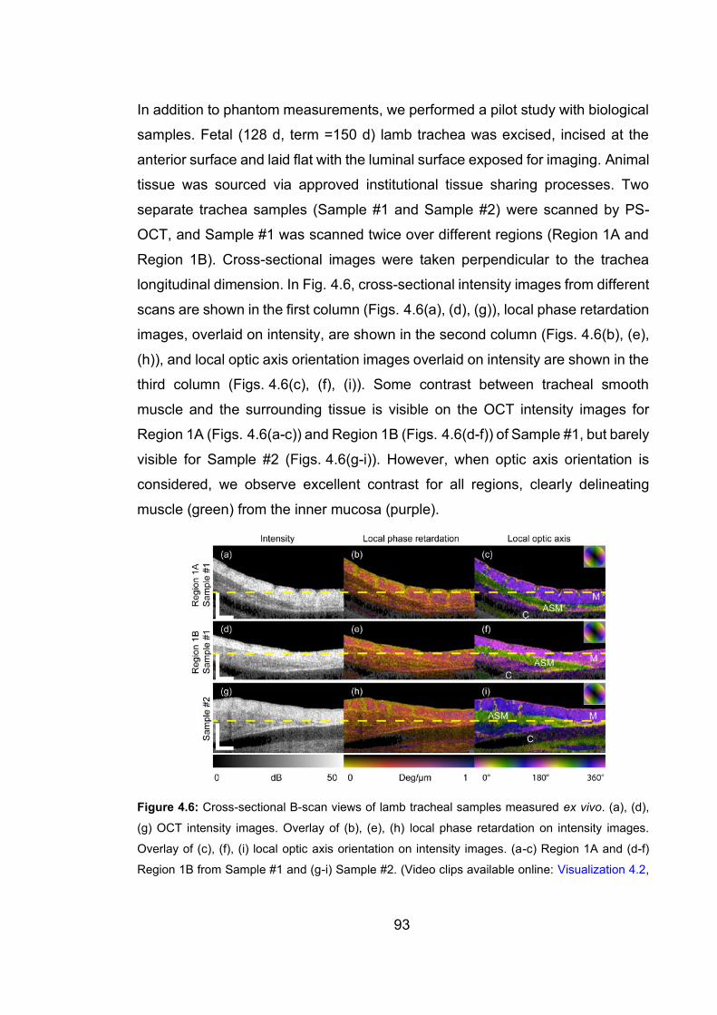
93
In addition to phantom measurements, we performed a pilot study with biological
samples. Fetal (128 d, term =150 d) lamb trachea was excised, incised at the
anterior surface and laid flat with the luminal surface exposed for imaging. Animal
tissue was sourced via approved institutional tissue sharing processes. Two
separate trachea samples (Sample #1 and Sample #2) were scanned by PS-
OCT, and Sample #1 was scanned twice over different regions (Region 1A and
Region 1B). Cross-sectional images were taken perpendicular to the trachea
longitudinal dimension. In Fig. 4.6, cross-sectional intensity images from different
scans are shown in the first column (Figs. 4.6(a), (d), (g)), local phase retardation
images, overlaid on intensity, are shown in the second column (Figs. 4.6(b), (e),
(h)), and local optic axis orientation images overlaid on intensity are shown in the
third column (Figs. 4.6(c), (f), (i)). Some contrast between tracheal smooth
muscle and the surrounding tissue is visible on the OCT intensity images for
Region 1A (Figs. 4.6(a-c)) and Region 1B (Figs. 4.6(d-f)) of Sample #1, but barely
visible for Sample #2 (Figs. 4.6(g-i)). However, when optic axis orientation is
considered, we observe excellent contrast for all regions, clearly delineating
muscle (green) from the inner mucosa (purple).
Figure 4.6: Cross-sectional B-scan views of lamb tracheal samples measured ex vivo. (a), (d),
(g) OCT intensity images. Overlay of (b), (e), (h) local phase retardation on intensity images.
Overlay of (c), (f), (i) local optic axis orientation on intensity images. (a-c) Region 1A and (d-f)
Region 1B from Sample #1 and (g-i) Sample #2. (Video clips available online: Visualization 4.2,

94
Visualization 4.3, and Visualization 4.4). M: Mucosa; ASM: Airway smooth muscle; C: Cartilage.
Scale bar: 500 μm (physical length).
Some indication of the orientation of the fibrous structures in different layers of
the lamb trachea is observable in the OCT intensity images when en face
projection (without flattening in post-processing) is used (Figs. 4.7(a), (d), (g)).
Local phase retardation mapping offers rather homogeneous images of the same
en face layers (Figs. 4.7(b), (e), (h)); whereas, local optic axis mapping provides
excellent contrast (Figs. 4.7(c), (f), (i)).
Figure 4.7: En face views of lamb trachea samples measured ex vivo. OCT intensity, local phase
retardation and local optic axis for: Regions 1A (a-c) and 1B (d-f) of Sample #1 and Sample #2
(g-i), corresponding to the layers indicated by the dashed yellow lines in Fig. 6, respectively. The
dashed cyan lines indicate the locations of the B-scan in Fig. 6. The localized blue region in (b)
and small white regions in (e) and (h) are artifacts due to strong reflections from the sample
surface. M: Mucosa; ASM: Airway smooth muscle. (Video clips available online: Visualization 4.5,
Visualization 4.6, and Visualization 4.7). Scale bar: 500 μm (physical length).
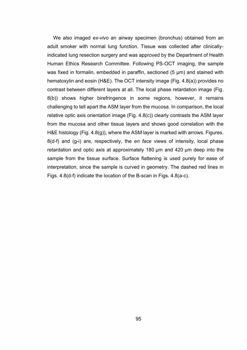
95
We also imaged ex-vivo an airway specimen (bronchus) obtained from an
adult smoker with normal lung function. Tissue was collected after clinically-
indicated lung resection surgery and was approved by the Department of Health
Human Ethics Research Committee. Following PS-OCT imaging, the sample
was fixed in formalin, embedded in paraffin, sectioned (5 μm) and stained with
hematoxylin and eosin (H&E). The OCT intensity image (Fig. 4.8(a)) provides no
contrast between different layers at all. The local phase retardation image (Fig.
8(b)) shows higher birefringence in some regions, however, it remains
challenging to tell apart the ASM layer from the mucosa. In comparison, the local
relative optic axis orientation image (Fig. 4.8(c)) clearly contrasts the ASM layer
from the mucosa and other tissue layers and shows good correlation with the
H&E histology (Fig. 4.8(g)), where the ASM layer is marked with arrows. Figures.
8(d-f) and (g-i) are, respectively, the en face views of intensity, local phase
retardation and optic axis at approximately 180 μm and 420 μm deep into the
sample from the tissue surface. Surface flattening is used purely for ease of
interpretation, since the sample is curved in geometry. The dashed red lines in
Figs. 4.8(d-f) indicate the location of the B-scan in Figs. 4.8(a-c).
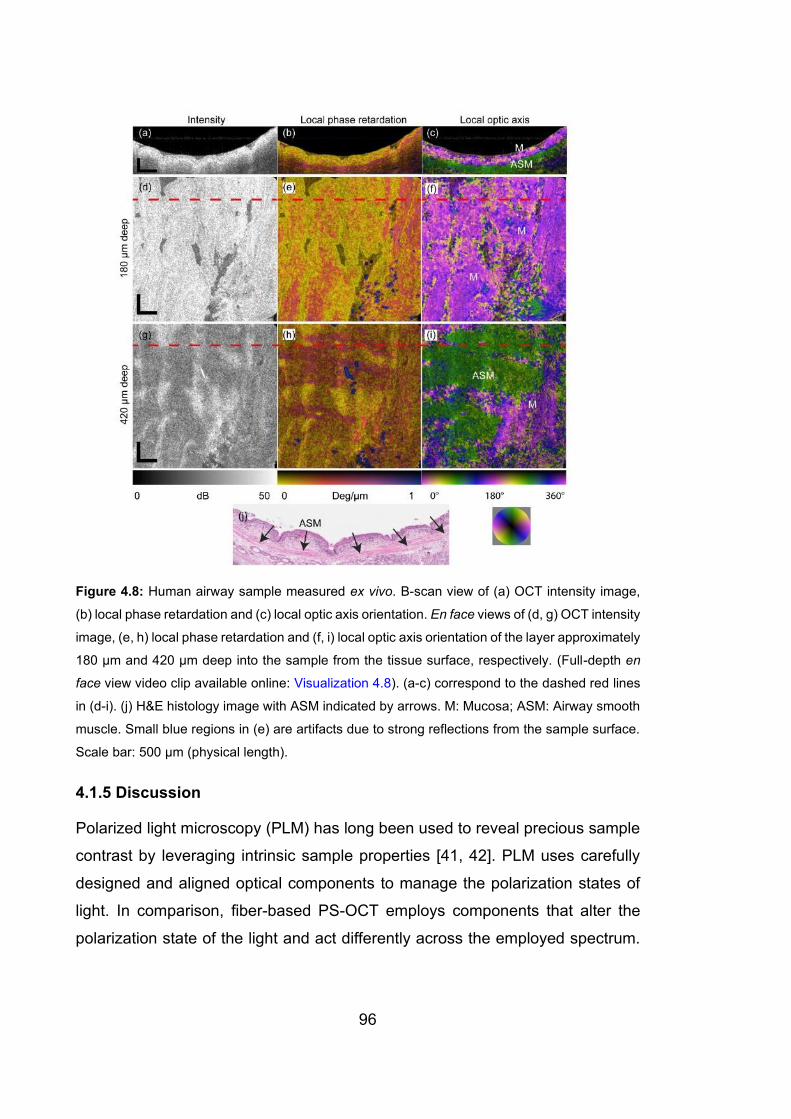
96
Figure 4.8: Human airway sample measured ex vivo. B-scan view of (a) OCT intensity image,
(b) local phase retardation and (c) local optic axis orientation. En face views of (d, g) OCT intensity
image, (e, h) local phase retardation and (f, i) local optic axis orientation of the layer approximately
180 μm and 420 μm deep into the sample from the tissue surface, respectively. (Full-depth en
face view video clip available online: Visualization 4.8). (a-c) correspond to the dashed red lines
in (d-i). (j) H&E histology image with ASM indicated by arrows. M: Mucosa; ASM: Airway smooth
muscle. Small blue regions in (e) are artifacts due to strong reflections from the sample surface.
Scale bar: 500 μm (physical length).
4.1.5 Discussion
Polarized light microscopy (PLM) has long been used to reveal precious sample
contrast by leveraging intrinsic sample properties [41, 42]. PLM uses carefully
designed and aligned optical components to manage the polarization states of
light. In comparison, fiber-based PS-OCT employs components that alter the
polarization state of the light and act differently across the employed spectrum.
97
The method presented in this manuscript estimates wavelength-dependent
correction terms, thereby improving on these deficiencies. The estimation is
performed directly on sample data, without specific requirements on sample
properties and without the need for specific calibration signals.
Comparisons of the optic axis orientation at three distinct regions of a
birefringence phantom suggest better robustness of the method in this
manuscript (red in Figs. 4.5(d-e)) than the one in Villiger et al. [25] (blue in Figs.
4.5(d-e)). The advantages of the approach proposed here are: i) the corrections
are made in the k-domain, so the axial resolution of the system is preserved,
which is especially important in resolving thin structures of thickness close to the
OCT axial resolution; ii) the diattenuation of the system is taken into account and,
therefore, the errors introduced by ignoring diattenuation are avoided and the
effort of aligning the reference signal is minimized; iii) unlike those systems that
require probing beam(s) with circular polarization states, the method requires no
alignment of input polarization states on the sample, and its extraction of the
relevant polarization parameters is robust, which might be beneficial for future
clinical applications, where careful alignment procedures are impractical.
In our system, the polarization-diverse optical mixer is a compact commercial
product, which prevents us from inserting a linear polarizer to filter the reference
signal to have identical power and phase for the orthogonal detection channels.
As a result, it is the dominant source of apparent system diattenuation. However,
in a system where the reference signal is polarized and correctly aligned, we
suggest making the Jones matrix symmetric with a correction matrix on the right-
hand side of Jtot(k), canceling Jin(k) instead of Jout(k). This would correct more
efficiently for an imbalance in the PDU, where the ratio of the power in the two
orthogonal polarized illumination beams might drift over time. In our case, we
carefully aligned the PDU before taking measurements, such that the two
illumination beams had equal power onto the sample. As a result, Jin(k) featured
minimal diattenuation that could be simply ignored. To further improve the
robustness to system drift and polarization dependent loss, it would be possible

98
to estimate the residual system diattenuation present in Jin(k) by minimizing the
cumulative diattenuation of J″tot(z) across an entire B-scan, under the assumption
that the sample itself is free of diattenuation. In this work, we also implicitly
assumed that the sample retardation is independent of the wavelength, i.e., the
same phase retardation is measured across all spectral bins. The same
assumption is made when reconstructing conventional PS-OCT images without
spectral binning. Yet, the correction for the k-dependence of the system
components relies on their effects being constant in time. k-dependence of the
sample retardation, if sufficiently varying in orientation across a B-scan, should
not significantly impact the ability to correct for the system transmission.
According to Park et al. [35], for fiber-based PS-OCT, there exists an inherent
ambiguity in the sign of the relative optic axis orientation. Although there is a
unique solution to the symmetrization of the polarization measurements, there
remains an ambiguity in the sign of the matrix root when computing Q0, which
corresponds to a ‘flip’ of the QU-plane of the Poincaré sphere. A straightforward
calibration step allows removing this sign ambiguity, whereby a birefringence
phantom with at least two distinct, non-orthogonal, and a priori known optic axis
orientations is imaged. Matching the sense of the relative axis orientations readily
provides the required sign to correctly interpret the axis orientations, as illustrated
in Fig. 4.4, and remains consistent until the system retardance is altered.
Once the sign ambiguity is removed, it is possible to convert the relative local
optic axis orientation, as measured here, to absolute local optic axis orientation
if the orientation of any layer is known and, thus, serves as a reference for the
entire sample, as in Fig. 4.5. Yet, in many cases, the relative optic axis orientation
provides sufficient information to differentiate layers of the sample and renders
unnecessary the need for absolute optic axis orientation. Additionally, we found
that in our system the relative orientation of the optic axis remained unchanged
with respect to the laboratory frame, even over periods of several days, as long
as the system components and fibers remained untouched. Therefore, we
anticipate that calibration with a polarization element once per measurement
99
session may well be sufficient to provide a measure of absolute optic axis
orientation.
The optic axis identified by our processing corresponds to a right-handed
rotation in the Poincaré space with right-hand circularly polarized light (looking
against the source) located at [Q, U, V]T = [0, 0, 1]T, and identifies the slow, i.e.,
retarding, axis of the birefringent material [36]. Biological birefringent tissues,
such as collagen and muscle, feature positive birefringence and, hence, the slow
axis corresponds to their extraordinary refractive index aligned along their fiber
direction [43]. Optic axis imaging in such tissues, as in Figs. 4.5-4.8, provides
excellent contrast between layers with different orientations. Local phase
retardation imaging, however, might fail to contrast such layers if they have
similar birefringence. Additionally, tensile or compressional stress of the sample,
occurring in preparation or in situ, might influence the amount of birefringence
with unknown effect, but should, in principle, not change the local optic axis
orientations of any layers in the sample. For tissues without birefringence, the
local SO(3) becomes close to the identity matrix, whose optic axis orientation is
undefined. Practically, the residual noise ensures that the resulting optic axis
orientation is, indeed, randomly oriented. The higher the birefringence of a
sample, the more trustworthy is the measured optic axis orientation. Hence, it is
possible to use the local phase retardation as a mask to suppress regions with
low/no birefringence. However, our samples were sufficiently retarding
throughout that we did not use this strategy. In Fig. 4.7, the inner mucosa has,
indeed, lower birefringence than the smooth muscle, but still features sufficient
birefringence to produce reliable optic axis maps.
With the current unoptimized code running on MATLAB R2016b, the
processing time is on average 2.0 s per B-scan (consisting of 1000 A-lines and
computing 1.2 mm in depth) on a desktop equipped with an Intel CPU (i7-7700
@3.6GHz) and with 32GB RAM. The symmetrization correction matrix Jcor(k) and
system polarization distortion compensation matrix Jcomp(k) are both estimated
from only a single B-scan at the beginning of the processing and directly applied

100
to all the other B-scans in the dataset. It takes approximately 19 s to find Jcor(k)
and Jcomp(k). Total time to process a 3D data set (1000 × 1000 A-lines) currently
is approximately 30 min for computing 1.2 mm in depth and 63 min for computing
5.0 mm in depth. To maximize the computing efficiency, we first crop the data
volume based on its 3D intensity, and then compute the optic axis only to a certain
depth, which is typically less than 2.0 mm, depending on the thickness of the
measured sample. We expect that the reconstruction could be significantly
accelerated by improving the numerical implementation and using parallel
processing with a graphics card.
4.1.6 Conclusions
We have developed a robust method for local phase retardation and local relative
optic axis orientation imaging that corrects for general system imperfections and
maintains the full axial resolution, based on a depth-multiplexed PS-OCT system
that simultaneously measures the full Jones matrix. We validated this method
with birefringence phantoms and demonstrated imaging of lamb trachea and
human airway samples ex vivo. We demonstrated it as a promising method for
segmenting ASM from other wall structures, which, with further validation, may
be a useful tool to study ASM remodeling in asthma.
Appendix A. Concurrent decomposition of a general Jones matrix into
simultaneously acting retardation and diattenuation vectors
A general Jones matrix is defined, to within an arbitrary phase and scaling term,
as:
3 3
1 1
1 1exp ,
2 2n n n n
n n
i r d = =
= − +
J (4.10)
where n = 1, 2, 3. Real-valued r1, r2 and r3 correspond, respectively, to the Q, U,
V components of a retardation vector r = [r1, r2, r3]T. Similarly, real-valued d1, d2
and d3 correspond, respectively, to a diattenuation vector d = [d1, d2, d3]T. σn is
the Pauli basis (n=0, 1, 2, 3):
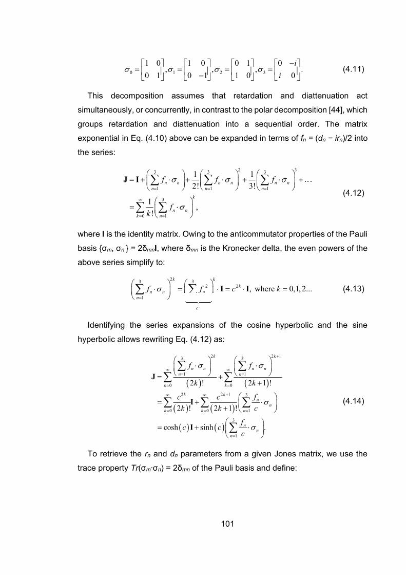
101
0 1 2 3
1 0 1 0 0 1 0, , , .
0 1 0 1 1 0 0
i
i
− = = = =
− (4.11)
This decomposition assumes that retardation and diattenuation act
simultaneously, or concurrently, in contrast to the polar decomposition [44], which
groups retardation and diattenuation into a sequential order. The matrix
exponential in Eq. (4.10) above can be expanded in terms of fn = (dn − irn)/2 into
the series:
2 33 3 3
1 1 1
3
0 1
1 1
2! 3!
1 ,
!
n n n n n n
n n n
k
n n
k n
f f f
fk
= = =
= =
= + + + +
=
J I
(4.12)
where I is the identity matrix. Owing to the anticommutator properties of the Pauli
basis {σm, σn } = 2δmnI, where δmn is the Kronecker delta, the even powers of the
above series simplify to:
2
23 3
2 2
1 1
, where 0,1,2...
k k
k
n n n
n n
c
f f c k= =
= = =
I I (4.13)
Identifying the series expansions of the cosine hyperbolic and the sine
hyperbolic allows rewriting Eq. (4.12) as:
( ) ( )
( ) ( )
( ) ( )
2 2 13 3
1 1
0 0
2 2 1 3
0 0 1
3
1
2 ! 2 1 !
2 ! 2 1 !
cosh sinh .
k k
n n n n
n n
k k
k k
nn
k k n
nn
n
f f
k k
fc c
k k c
fc c
c
+
= =
= =
+
= = =
=
= +
+
= +
+
= +
J
I
I
(4.14)
To retrieve the rn and dn parameters from a given Jones matrix, we use the
trace property Tr(σm∙σn) = 2δmn of the Pauli basis and define:
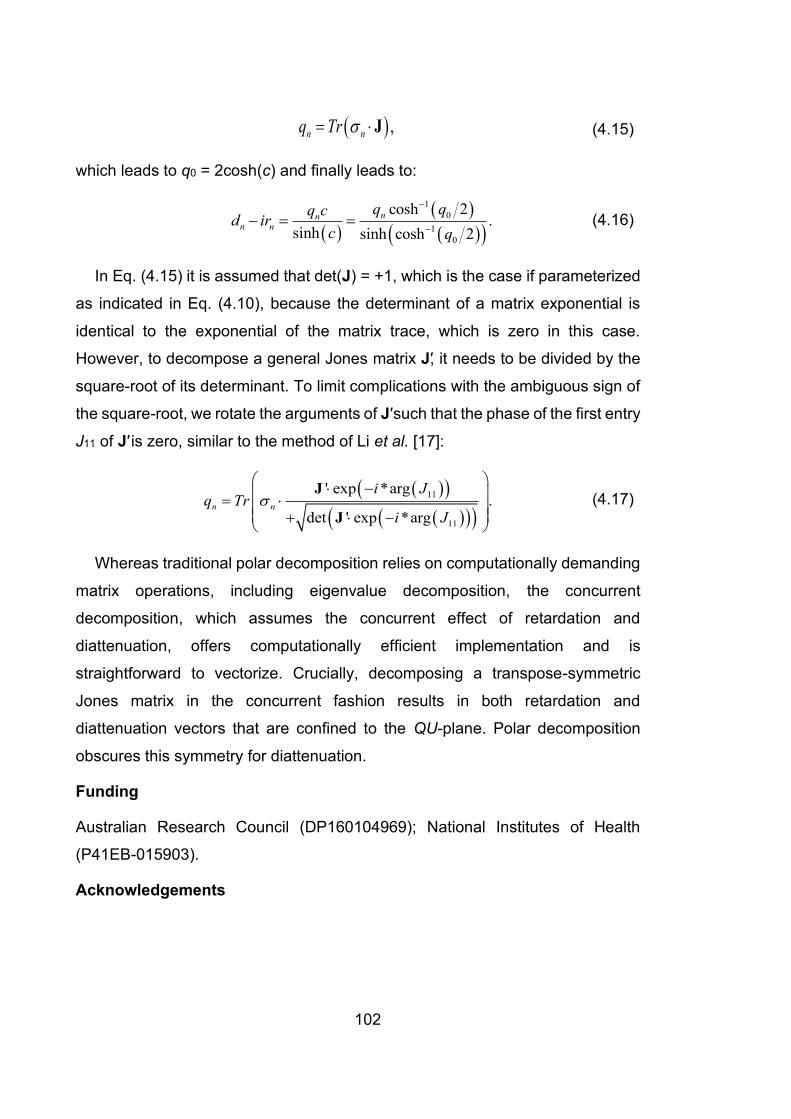
102
( ) ,n nq Tr = J (4.15)
which leads to q0 = 2cosh(c) and finally leads to:
( )
( )
( )( )
1
0
1
0
cosh 2.
sinh sinh cosh 2
nnn n
q qq cd ir
c q
−
−− = = (4.16)
In Eq. (4.15) it is assumed that det(J) = +1, which is the case if parameterized
as indicated in Eq. (4.10), because the determinant of a matrix exponential is
identical to the exponential of the matrix trace, which is zero in this case.
However, to decompose a general Jones matrix J′, it needs to be divided by the
square-root of its determinant. To limit complications with the ambiguous sign of
the square-root, we rotate the arguments of J′ such that the phase of the first entry
J11 of J′ is zero, similar to the method of Li et al. [17]:
( )( )
( )( )( )11
11
' exp *arg.
det ' exp *argn n
i Jq Tr
i J
− =
+ −
J
J
(4.17)
Whereas traditional polar decomposition relies on computationally demanding
matrix operations, including eigenvalue decomposition, the concurrent
decomposition, which assumes the concurrent effect of retardation and
diattenuation, offers computationally efficient implementation and is
straightforward to vectorize. Crucially, decomposing a transpose-symmetric
Jones matrix in the concurrent fashion results in both retardation and
diattenuation vectors that are confined to the QU-plane. Polar decomposition
obscures this symmetry for diattenuation.
Funding
Australian Research Council (DP160104969); National Institutes of Health
(P41EB-015903).
Acknowledgements

103
Q. Li would like to acknowledge the financial support of the Australian
Government International Research Training Program (RTP) Fee Offset
Scholarships.
Disclosures
The authors declare that there are no conflicts of interest related to this article.
References for Section 4.1
1. D. Huang, E. A. Swanson, C. P. Lin, J. S. Schuman, W. G. Stinson, W. Chang,
M. R. Hee, T. Flotte, K. Gregory, C. A. Puliafito, and J. G. Fujimoto, “Optical
coherence tomography,” Science 254(5035), 1178‒1181 (1991).
2. K. V. Larin and D. D. Sampson, “Optical coherence elastography - OCT at
work in tissue biomechanics [Invited],” Biomed. Opt. Express 8(2), 1172‒1202
(2017).
3. B. F. Kennedy, P. Wijesinghe, and D. D. Sampson, “The emergence of optical
elastography in biomedicine,” Nat. Photon. 11, 215 (2017).
4. C.-L. Chen and R. K. Wang, “Optical coherence tomography based
angiography [Invited],” Biomed. Opt. Express 8(2), 1056‒1082 (2017).
5. P. Gong, S. Es'haghian, K. A. Harms, A. Murray, S. Rea, B. F. Kennedy, F.
M. Wood, D. D. Sampson, and R. A. McLaughlin, “Optical coherence
tomography for longitudinal monitoring of vasculature in scars treated with
laser fractionation,” J. Biophotonics 9(6), 626‒636 (2015).
6. J. F. de Boer, C. K. Hitzenberger, and Y. Yasuno, “Polarization sensitive
optical coherence tomography - a review [Invited],” Biomed. Opt. Express 8(2),
1838-‒1873 (2017).
7. B. Baumann, “Polarization sensitive optical coherence tomography: a review
of technology and applications,” Appl. Sci. 7(5), 474 (2017).
8. B. Cense, T. C. Chen, B. H. Park, M. C. Pierce, and J. F. de Boer, “In vivo
depth-resolved birefringence measurements of the human retinal nerve fiber
104
layer by polarization-sensitive optical coherence tomography,” Opt. Lett.
27(18), 1610‒1612 (2002).
9. M. Pircher, C. K. Hitzenberger, and U. Schmidt-Erfurth, “Polarization sensitive
optical coherence tomography in the human eye,” Prog. Retin. Eye Res.
30(6), 431–451 (2011).
10. T. Louie, C. Lee, D. Hsu, K. Hirasuna, S. Manesh, M. Staninec, C. L. Darling,
and D. Fried, “Clinical assessment of early tooth demineralization using
polarization sensitive optical coherence tomography,” Lasers in Surg. Med.
42(10), 898‒905 (2010).
11. W. C. Lo, M. Villiger, A. Golberg, G. F. Broelsch, S. Khan, C. G. Lian, W. G.
Austen, Jr., M. Yarmush, and B. E. Bouma, “Longitudinal, 3D Imaging of
Collagen Remodeling in Murine Hypertrophic Scars In Vivo Using
Polarization-Sensitive Optical Frequency Domain Imaging,” J. Invest.
Dermatol. 136(1), 84‒92 (2016).
12. P. Gong, L. Chin, S. Es'haghian, Y. M. Liew, F. M. Wood, D. D. Sampson,
and R. A. McLaughlin, “Imaging of skin birefringence for human scar
assessment using polarization-sensitive optical coherence tomography aided
by vascular masking,” J. Biomed. Opt. 19(12), 126014 (2014).
13. E. Li, S. Makita, Y.-J. Hong, D. Kasaragod, and Y. Yasuno, “Three-
dimensional multi-contrast imaging of in vivo human skin by Jones matrix
optical coherence tomography,” Biomed. Opt. Express 8(3), 1290‒1305
(2017).
14. H. Wang, A. J. Black, J. Zhu, T. W. Stigen, M. K. Al-Qaisi, T. I. Netoff, A.
Abosch, and T. Akkin, “Reconstructing micrometer-scale fiber pathways in the
brain: Multi-contrast optical coherence tomography based tractography,”
Neuroimage 58(4), 984‒992 (2011).
15. H. Wang, T. Akkin, C. Magnain, R. Wang, J. Dubb, W. J. Kostis, M. A. Yaseen,
A. Cramer, S. Sakadžić, and D. Boas, “Polarization sensitive optical

105
coherence microscopy for brain imaging,” Opt. Lett. 41(10), 2213‒2216
(2016).
16. M. Villiger, K. Otsuka, A. Karanasos, P. Doradla, J. Ren, N. Lippok, M.
Shishkov, J. Daemen, R. Diletti, R.-J. van Geuns, F. Zijlstra, G. van Soest, P.
Libby, E. Regar, S. K. Nadkarni, and B. E. Bouma, “Coronary plaque
microstructure and composition modify optical polarization: a new
endogenous contrast mechanism for optical frequency domain imaging,”
JACC: Cardiovasc. Imag., Dec., e-pub ahead of print (2017).
17. J. Li, F. Feroldi, J. de Lange, J. M. A. Daniels, K. Grünberg, and J. F. de Boer,
“Polarization sensitive optical frequency domain imaging system for
endobronchial imaging,” Opt. Express 23(3), 3390‒3402 (2015).
18. D. C. Adams, L. P. Hariri, A. J. Miller, Y. Wang, J. L. Cho, M. Villiger, J. A.
Holz, M. V. Szabari, D. L. Hamilos, R. Scott Harris, J. W. Griffith, B. E. Bouma,
A. D. Luster, B. D. Medoff, and M. J. Suter, “Birefringence microscopy
platform for assessing airway smooth muscle structure and function in vivo,”
Sci. Transl. Med. 8, 359ra131 (2016).
19. C. Fan and G. Yao, “Mapping local retardance in birefringent samples using
polarization sensitive optical coherence tomography,” Opt. Lett. 37(9), 1415‒
1417 (2012).
20. C. Fan and G. Yao, “Imaging myocardial fiber orientation using polarization
sensitive optical coherence tomography,” Biomed. Opt. Express 4(3), 460‒
465 (2013).
21. M. Todorović, S. Jiao, L. V. Wang, and G. Stoica, “Determination of local
polarization properties of biological samples in the presence of diattenuation
by use of Mueller optical coherence tomography,” Opt. Lett. 29(20), 2402–
2404 (2004).
22. L. Azinfar, M. Ravanfar, Y. Wang, K. Zhang, D. Duan, and G. Yao, “High
resolution imaging of the fibrous microstructure in bovine common carotid
106
artery using optical polarization tractography,” J. Biophotonics 10(2), 231‒241
(2017).
23. Y. Wang, K. Zhang, N. B. Wasala, D. Duan, and G. Yao, “Optical polarization
tractography revealed significant fiber disarray in skeletal muscles of a mouse
model for Duchenne muscular dystrophy,” Biomed. Opt. Express 6(2), 347‒
352 (2015).
24. Y. Wang, M. Ravanfar, K. Zhang, D. Duan, and G. Yao, “Mapping 3D fiber
orientation in tissue using dual-angle optical polarization tractography,”
Biomed. Opt. Express 7(10), 3855‒3870 (2016).
25. M. Villiger, B. Braaf, N. Lippok, K. Otsuka, S. K. Nadkarni, and B. E. Bouma,
“Optic axis mapping with catheter-based polarization-sensitive optical
coherence tomography, ” Optica 5(10), 1329‒1337 (2018).
26. Y. S. Prakash, “Emerging concepts in smooth muscle contributions to airway
structure and function: implications for health and disease,” Am. J. Physiol.
Lung Cell Mol. Physiol. 311(6), L1113‒L1140 (2016).
27. G. M. Donovan, J. G. Elliot, F. H. Y. Green, A. L. James, and P. B. Noble,
“Unravelling a clinical paradox - why does bronchial thermoplasty work in
asthma?” Am. J. of Respir. Cell Mol. Biol. 59(3), 355‒362; e-pub ahead of
print (2018).
28. M. Villiger, D. Lorenser, R. A. McLaughlin, B. C. Quirk, R. W. Kirk, B. E.
Bouma, and D. D. Sampson, “Deep tissue volume imaging of birefringence
through fibre-optic needle probes for the delineation of breast tumour,” Sci.
Rep. 6(1), 28771 (2016).
29. B. Baumann, W. Choi, B. Potsaid, D. Huang, J. S. Duker, and J. G. Fujimoto,
“Swept source/Fourier domain polarization sensitive optical coherence
tomography with a passive polarization delay unit,” Opt. Express 20(9),
10229‒10241 (2012).
30. Y. Lim, Y.-J. Hong, L. Duan, M. Yamanari, and Y. Yasuno, “Passive
component based multifunctional Jones matrix swept source optical
107
coherence tomography for Doppler and polarization imaging,” Opt. Lett.
37(11), 1958‒1960 (2012).
31. B. Braaf, K. A. Vermeer, M. de Groot, K. V. Vienola, and J. F. de Boer, “Fiber-
based polarization-sensitive OCT of the human retina with correction of
system polarization distortions,” Biomed. Opt. Express 5(8), 2736‒2758
(2014).
32. M. Villiger, E. Z. Zhang, S. K. Nadkarni, W.-Y. Oh, B. J. Vakoc, and B. E.
Bouma, “Spectral binning for mitigation of polarization mode dispersion
artifacts in catheter-based optical frequency domain imaging,” Opt. Express
21(14), 16353‒16369 (2013).
33. N. Vansteenkiste, P. Vignolo, and A. Aspect, “Optical reversibility theorems
for polarization: application to remote control of polarization,” J. Opt. Soc. Am.
A 10(10), 2240–2245 (1993).
34. S.-Y. Lu and R. A. Chipman, “Interpretation of Mueller matrices based on
polar decomposition,” J. Opt. Soc. Am. A 13(5), 1106‒1113 (1996).
35. B. H. Park, M. C. Pierce, B. Cense, and J. F. de Boer, “Optic axis
determination accuracy for fiber-based polarization-sensitive optical
coherence tomography,” Opt. Lett. 30(19), 2587‒2589 (2005).
36. J. P. Gordon and H. Kogelnik, “PMD fundamentals: Polarization mode
dispersion in optical fibers,” Proc. Natl. Acad. Sci. 97(9), 4541‒4550 (2000).
37. J. Li and J. F. de Boer, “Coherent signal composition and global phase
determination in signal multiplexed polarization sensitive optical coherence
tomography,” Opt. Express 22(18), 21382‒21392 (2014).
38. Y. Furuhashi, Y. Kimura, and H. Yamane, “Higher order structural analysis of
stereocomplex‐type poly (lactic acid) melt‐spun fibers,” J. Polym. Sci. B:
Polym. Phys. 45(2), 218‒228 (2007).
108
39. N. Lippok, M. Villiger, and B. E. Bouma, “Degree of polarization (uniformity)
and depolarization index: unambiguous depolarization contrast for optical
coherence tomography,” Opt. Lett. 40(17), 3954‒3957 (2015).
40. J. Schindelin, I. Arganda-Carreras, E. Frise, V. Kaynig, M. Longair, T.
Pietzsch, S. Preibisch, C. Rueden, S. Saalfeld, B. Schmid, J.-Y. Tinevez, D.
J. White, V. Hartenstein, K. Eliceiri, P. Tomancak, and A. Cardona, “Fiji: an
open-source platform for biological-image analysis,” Nat. Methods 9, 676
(2012).
41. R. Oldenbourg, “A new view on polarization microscopy,” Nature 381, 811‒
812 (1996).
42. R. A. Carlton, “Polarized Light Microscopy,” in Pharmaceutical Microscopy, R.
A. Carlton, ed. (Springer New York, New York, NY, 2011), pp. 7‒64.
43. M. Wolman, “Polarized light microscopy as a tool of diagnostic pathology,” J.
Histochem. Cytochem. 23(1), 21–50 (1975).
44. Tudor, “Vectorial Pauli algebraic approach in polarization optics. I. Device and
state operators,” Optik 121(13), 1226‒1235 (2010).
4.2 ROTATING CATHETER-BASED CONFIGURATION
Previously, Villiger et al. [56] demonstrated that the local optic axis orientation of
sample can be recovered in a rotating catheter-based PS-OCT system for
endoscopic applications. Here, we also extend our robust processing from
standard bench-top to rotating catheter-based configuration and demonstrate the
capacity to differentiate smooth muscle layers in in-tact porcine airway samples
ex-vivo.
A home-made ball-lens catheter with ~1.0 m length replaced the standard
microscope configuration for this experiment. Single-mode fibres were used in
the system throughout, including within the catheter. A commercial rotary joint
linked the catheter and the static part of the OCT system and provided
unidirectional rotation of the catheter at ~2.0 rev/s. The rotary joint was mounted

109
on a translation stage that provided pullback of the catheter at ~25 μm/s for 3D
volumetric scanning. The ball lens at the distal end of the catheter was 400 μm
in diameter and approximately half of the ball was removed by polishing at 45˚.
The catheter provided a working distance of 1.15 mm from its centre, a DOF of
266 μm and lateral resolution of 15 μm. The ball lens was protected by a thin,
hollow, cylindrical metal cap with ~600 μm outer diameter, into which a window
was drilled for the side-viewing purposes. The entire catheter rotated inside a
transparent plastic tubing, whose inner and outer diameters were 1.2 mm and 2.0
mm, respectively. Fresh, hollow ex-vivo porcine airway samples a few
centimetres in length were scanned by inserting the plastic tubing inside the
lumen of the samples. Fig. 4.9 shows a simple schematic of the ball-lens structure.
Figure 4.9: A simple schematic of the home-made catheter with ball lens structure. SMF, single-
mode fibre.
The imaging source was upgraded to a newer model with a broader spectral
bandwidth of ~ 130 nm, improving the axial resolution to 11 μm in air. Due to the
relatively slow scanning speed, only 10% of the A-lines of the source were used
for imaging, which essentially reduces the effective A-line rate from 50 kHz down
to 5 kHz.
The same processing algorithm as [56] was applied here, except that all the
system distortions (including diattenuation components) were corrected in the
original wavenumber domain rather than in SO(3) domain, which maintained the
system axial resolution.

110
In brief, the outer surface of the ball lens provided an additional reference
signal that allowed estimation of the system transmission matrices. The
measured Jones matrix Jtot(k, θ) with a rotating catheter has two additional
elements compared to the measurement from a static system, i.e., R(θ) and Jcat,
as seen in Eq. 4.18:
( )
( ) ( ) ( ) ( ) ( ) ( ) ( )
tot
out cat sam sam cat in0
,
exp 2 .T T T
k
k z z i k z dz k
=
J
J R J J J J R J (4.18)
Note that here Jtot(k, θ) not only varies with wavenumber k, but also the angular
orientation (between 0 and 2π) of the catheter θ. R(θ) is a θ-dependent circular
retarding matrix resulting from the coordinate change due to rotation of the
catheter, whereas Jcat denotes a constant transmission matrix of the catheter
from the rotary joint to the ball-lens surface.
With the same strategy as used in the static bench-top setup, the original
Jones matrices were transpose symmetrised first, and compensated for system
polarisation distortions, such that the k-dependence is removed, as in Eq. 4.19:
( )
( ) ( ) ( ) ( ) ( ) ( ) ( )
tot
in cat sam sam cat in0
exp 2 .T T T T
c ck z z i k z dz k
=
J
J R J J J J R J
(4.19)
To obtain access to the sample matrices, we had to remove the effects of the
rotating catheter, including R(θ) and Jcat. Here the Jones matrices of the catheter
due to the reflection of the ball-lens were used to estimate the unknown matrices,
Jin(kc), R(θ) and Jcat, following a similar strategy to that in [56], except that Jin(kc)
and Jcat are no longer assumed to be purely retarding, but also diattenuating,
although the amount of diattenuation is relatively small.
Firstly, the current Jones matrix of the catheter surface signal could be
expressed as below:
( ) ( ) ( ) ( ) ( )surf in cat cat in .T T T
c ck k = J J R J J R J (4.20)
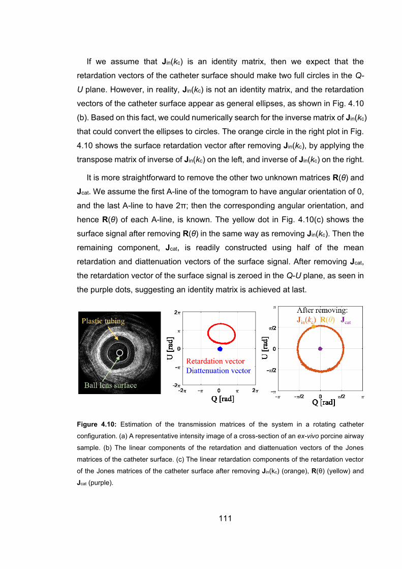
111
If we assume that Jin(kc) is an identity matrix, then we expect that the
retardation vectors of the catheter surface should make two full circles in the Q-
U plane. However, in reality, Jin(kc) is not an identity matrix, and the retardation
vectors of the catheter surface appear as general ellipses, as shown in Fig. 4.10
(b). Based on this fact, we could numerically search for the inverse matrix of Jin(kc)
that could convert the ellipses to circles. The orange circle in the right plot in Fig.
4.10 shows the surface retardation vector after removing Jin(kc), by applying the
transpose matrix of inverse of Jin(kc) on the left, and inverse of Jin(kc) on the right.
It is more straightforward to remove the other two unknown matrices R(θ) and
Jcat. We assume the first A-line of the tomogram to have angular orientation of 0,
and the last A-line to have 2π; then the corresponding angular orientation, and
hence R(θ) of each A-line, is known. The yellow dot in Fig. 4.10(c) shows the
surface signal after removing R(θ) in the same way as removing Jin(kc). Then the
remaining component, Jcat, is readily constructed using half of the mean
retardation and diattenuation vectors of the surface signal. After removing Jcat,
the retardation vector of the surface signal is zeroed in the Q-U plane, as seen in
the purple dots, suggesting an identity matrix is achieved at last.
Figure 4.10: Estimation of the transmission matrices of the system in a rotating catheter
configuration. (a) A representative intensity image of a cross-section of an ex-vivo porcine airway
sample. (b) The linear components of the retardation and diattenuation vectors of the Jones
matrices of the catheter surface. (c) The linear retardation components of the retardation vector
of the Jones matrices of the catheter surface after removing Jin(kc) (orange), R(θ) (yellow) and
Jcat (purple).
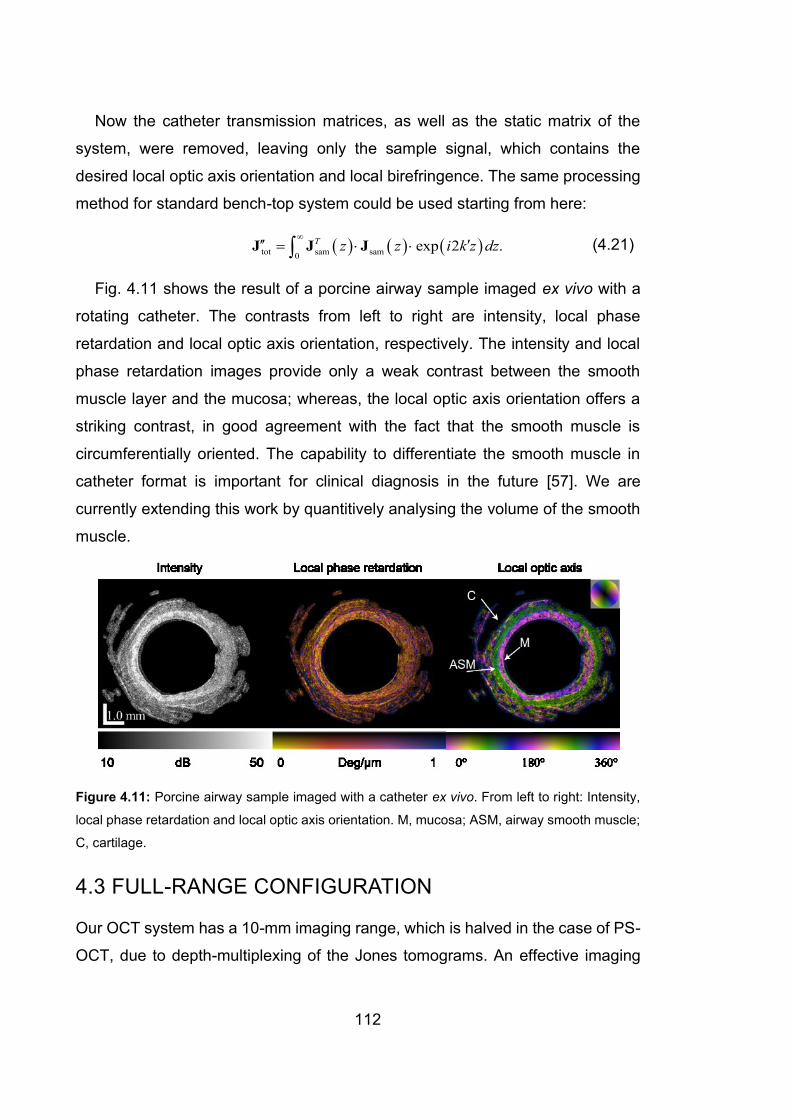
112
Now the catheter transmission matrices, as well as the static matrix of the
system, were removed, leaving only the sample signal, which contains the
desired local optic axis orientation and local birefringence. The same processing
method for standard bench-top system could be used starting from here:
( ) ( ) ( )tot sam sam0
exp 2 .T z z i k z dz
= J J J (4.21)
Fig. 4.11 shows the result of a porcine airway sample imaged ex vivo with a
rotating catheter. The contrasts from left to right are intensity, local phase
retardation and local optic axis orientation, respectively. The intensity and local
phase retardation images provide only a weak contrast between the smooth
muscle layer and the mucosa; whereas, the local optic axis orientation offers a
striking contrast, in good agreement with the fact that the smooth muscle is
circumferentially oriented. The capability to differentiate the smooth muscle in
catheter format is important for clinical diagnosis in the future [57]. We are
currently extending this work by quantitively analysing the volume of the smooth
muscle.
Figure 4.11: Porcine airway sample imaged with a catheter ex vivo. From left to right: Intensity,
local phase retardation and local optic axis orientation. M, mucosa; ASM, airway smooth muscle;
C, cartilage.
4.3 FULL-RANGE CONFIGURATION
Our OCT system has a 10-mm imaging range, which is halved in the case of PS-
OCT, due to depth-multiplexing of the Jones tomograms. An effective imaging

113
range of 5 mm is enough for most applications except for capturing the entire
anterior segment of human eye. Its large geometric curvature requires a detection
range of ~10 mm. Here, we adapted our system and doubled the imaging range
by introducing a simple full-range technique using an off-pivot scanning strategy,
developed over a decade ago [58, 59].
In brief, the collimated illumination beam in the sample arm, does not impinge
on the centre of the faster galvanometric mirror, but is laterally offset from it. By
doing so, a constant phase shift is induced between adjacent A-lines in a B-scan
that corresponds to adding a modulation in the lateral spatial domain. A simple
sketch of the probing beam geometry is shown in Fig. 4.12. The induced phase
difference between two adjacent A-lines is given as [58]:
max4,
s
N
=
(4.22)
where s is the offset of the mirror’s axis relative to the beam, max is the total
scanning angle of the mirror, N is the number of A-lines per B-scan, and is
the central wavelength of light source.
The offset is optimised to maximise the suppression ratio of the intensity of a
true image over its mirrored artefact, by monitoring in real time both the position
of the peak frequency in the spatial domain and the intensity of the mirror image,
with a custom-written C++ program. In principle, the highest suppression ratio
was reached when the induced phase shift between adjacent A-lines was / 2
[58, 59].

114
Figure 4.12: Sketch of probing beam geometry for full-range configuration. GM, Galvanometric
mirror. The illumination beam does not impinge on the centre of the galvanometric mirror, but is
offset by s. Adapted from [58].
By demodulating the interferograms in the spatial domain, we recovered the
imaginary part of the complex-valued interferogram that was otherwise not
measurable. Hence, the conjugate mirrored artefact in FD-OCT is removed and
the negative frequency region of z domain is also valid for imaging. To also
extend the lateral scanning range, a pair of large galvanometric mirrors (10 mm,
GVS112, Thorlabs Inc.) and a low N.A. objective lens (LSM05, Thorlabs Inc.) with
a large F.O.V (> 20 × 20 mm2) were used. An example of human palm image is
presented in Fig. 4.13 that compares the conventional and full-range processing.
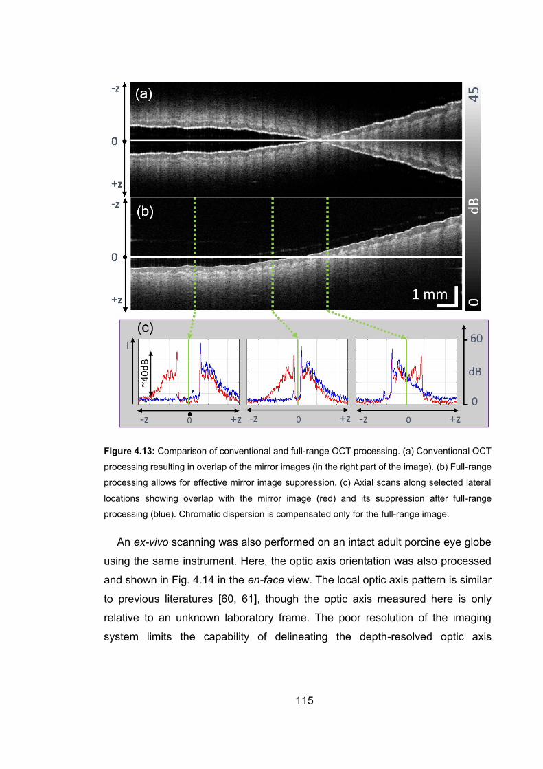
115
Figure 4.13: Comparison of conventional and full-range OCT processing. (a) Conventional OCT
processing resulting in overlap of the mirror images (in the right part of the image). (b) Full-range
processing allows for effective mirror image suppression. (c) Axial scans along selected lateral
locations showing overlap with the mirror image (red) and its suppression after full-range
processing (blue). Chromatic dispersion is compensated only for the full-range image.
An ex-vivo scanning was also performed on an intact adult porcine eye globe
using the same instrument. Here, the optic axis orientation was also processed
and shown in Fig. 4.14 in the en-face view. The local optic axis pattern is similar
to previous literatures [60, 61], though the optic axis measured here is only
relative to an unknown laboratory frame. The poor resolution of the imaging
system limits the capability of delineating the depth-resolved optic axis
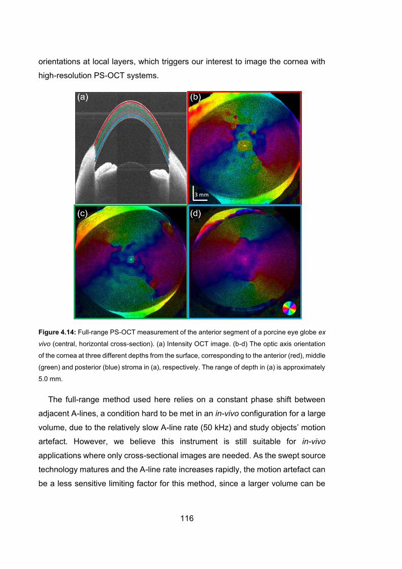
116
orientations at local layers, which triggers our interest to image the cornea with
high-resolution PS-OCT systems.
Figure 4.14: Full-range PS-OCT measurement of the anterior segment of a porcine eye globe ex
vivo (central, horizontal cross-section). (a) Intensity OCT image. (b-d) The optic axis orientation
of the cornea at three different depths from the surface, corresponding to the anterior (red), middle
(green) and posterior (blue) stroma in (a), respectively. The range of depth in (a) is approximately
5.0 mm.
The full-range method used here relies on a constant phase shift between
adjacent A-lines, a condition hard to be met in an in-vivo configuration for a large
volume, due to the relatively slow A-line rate (50 kHz) and study objects’ motion
artefact. However, we believe this instrument is still suitable for in-vivo
applications where only cross-sectional images are needed. As the swept source
technology matures and the A-line rate increases rapidly, the motion artefact can
be a less sensitive limiting factor for this method, since a larger volume can be
117
scanned in a shorter time. In contrast, the detection bandwidth and hence the
imaging range might not be enough to allow depth-multiplexing for high-speed
acquisitions, and doubling the imaging range with a simple, passive off-pivot
strategy, as demonstrated here, can be an interesting option.
Indeed, the phase shift induced between adjacent A-lines is chromatic.
Therefore, for high-resolution imaging applications, the full-range technique
might not work as reliably as demonstrated here, given the broad bandwidth of
the imaging light source.
In conclusion, the robust method developed for standard bench-top systems
can be readily applied in full-range configurations, where the doubled imaging
range through spatial domain demodulation allows imaging of the entire porcine
anterior segment. However, the lateral resolution of the system had to be
sacrificed to provide enough range of confocal gating to match the extended
range of coherence gating.
4.4 MULTI-FUNCTIONAL PS-OCT
Our PS-OCT is readily adaptable to provide other interesting sources of contrast.
For instance, by capturing two or more B-scans at the same location, we can map
the angiographic distributions based on the speckle decorrelation between the
multiple intensity images [62, 63]. In static tissues, the back-scattering intensity
is constant over time; whereas, the flowing blood in the vessel changes the
intensity. The collagen fibre distribution and the blood vessel architecture
together will allow a more comprehensive characterisation of the sample, which
is useful in diagnosing diseases, such as cancer.
Here, we followed our previous studies of the healthy human oral mucosa in
vivo [64]. The configuration of the imaging setup remained the same, i.e., a tilted
glass window was properly positioned after the objective lens, and in-vivo human
oral mucosa was attached directly onto the outer side of the glass window. The
scanning pattern of the galvanometric mirrors was adjusted accordingly such that
every single cross-section of the sample was scanned twice consecutively. The
intensity of a tomogram was computed by taking the magnitude of the

118
determinant of the Jones matrix, after numerical correction of system polarisation
distortions. Then the decorrelation of the two intensity tomograms of the same
cross-section, ( , , )D x y z , was computed for angiographic imaging, given by [62],
3 3
1 1
3 3 3 32 2
1 1 1 1
( , , )
( ( , , , ) ( , , , ))( ( , , , ) ( , , , ))
1 .
( ( , , , ) ( , , , )) ( ( , , , ) ( , , , ))
m n
m n m n
D x y z
I x m y z n t I x y z t I x m y z n t I x y z t
I x m y z n t I x y z t I x m y z n t I x y z t
= =
= = = =
=
+ + − + + − −
+ + − + + −
(4.23)
Here, I is the back-scattering intensity, I is the spatially filtered back-
scattering intensity, , ,x y z indicate the 3-D locations, and ,t t indicate the
different time points of the scanning.
The intensity, local OA orientation and the speckle decorrelation at different
depths of healthy human oral mucosa, measured in vivo, are shown in Fig. 4.15.
The local OA contrast is overlaid onto the local birefringence such that higher
birefringence has higher brightness, highlighting the collagen fibres. A
comprehensive characterisation is obtained by combining the collagen fibre
organisations from OA and the blood vessels from the speckle decorrelation.
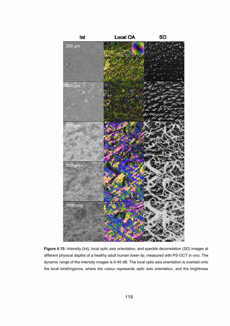
119
Figure 4.15: Intensity (Int), local optic axis orientation, and speckle decorrelation (SD) images at
different physical depths of a healthy adult human lower lip, measured with PS-OCT in vivo. The
dynamic range of the intensity images is 0-45 dB. The local optic axis orientation is overlaid onto
the local birefringence, where the colour represents optic axis orientation, and the brightness
120
represents the value of local birefringence. The field of view is 2.5 mm × 2.5 mm. The group
refractive index of the tissue is assumed to be n=1.4.
The angiographic images were acquired by simply repeating the lateral
scanning without physical modification of the system, and the blood vessels
revealed from these images, can significantly enrich our understanding of the
sample, especially if one combines the local optic axis orientation information as
well. We anticipate that the multi-contrasts from our PS-OCT provides a more
comprehensive characterisation of the structure of the sample, and may aid in
non-invasively detecting oral mucosal changes related to diseases, in particular,
oral cancer. Such studies are a natural extension of the preliminary
demonstration reported here.
4.5 SUMMARY
In this chapter, a robust method to retrieve local optic axis orientation with a
standard bench-top fibre-based PS-OCT system was developed and extended
to rotating catheter and full-range configurations. The algorithm corrects for
system polarisation distortions in the wavenumber domain and hence maintains
the axial resolution of the system. Smooth muscle was differentiated from the
surrounding tissues in airway samples, both in bench-top and catheter
configurations. A more comprehensive characterisation of living tissue was
demonstrated by combining the collagen fibre organisation from polarisation
contrast with the blood vessels obtained from angiography. Yet, the resolution of
the most PS-OCT systems, including those demonstrated in this chapter, is in the
order of 10 μm, which is not enough to resolve sample structures on the
micrometre scale such as stromal morphology. It is desirable to push the
resolution of PS-OCT to micrometre scale for imaging sample microstructures.
Attaining such high resolution based on swept source OCT has been a challenge,
because the current commercially available lasers lack the broad spectral
bandwidth for micrometre axial resolution. So, we decided to build a PS-OCM
system based on spectral domain OCT, by taking advantage of off-the-shelf

121
supercontinuum light source and twin spectrometers. We describe this system
and the remarkable images it is able to generate in the next chapter.
122
5 POLARISATION-SENSITIVE OPTICAL
COHERENCE MICROSCOPY
In earlier chapters, local polarisation contrasts have been investigated with PS-
OCT at conventional resolution on the order of 10 μm. Here, a micron-resolution,
PS-OCM is developed and presented, and shown capable of volumetrically
revealing the micro-morphology and fibre structures of sheep ocular tissues ex
vivo, using intensity and local optic axis orientations, respectively. Single-mode
fibres are used throughout the system, conveniently dividing the whole system
into several sub-units the alignment of which can be optimised separately. To
overcome the intrinsic trade-off between high lateral resolution and shallow depth
of field present with Gaussian optics, the illumination and detection beams were
decoupled, and the illumination beam was engineered to have a Bessel-like
shape by means of an axicon lens, that maintains high lateral resolution over an
extended depth of field. As in the conventional resolution setup, here, in the high-
resolution regime, the wavelength-dependent system polarisation distortions are
compensated in the wavenumber domain to remove system-induced artefacts.
The system is highly promising for imaging human cornea in vivo, especially if a
more appropriate light source is used.
123
5.1 VECTORIAL BIREFRINGENCE IMAGING BY OPTICAL
COHERENCE MICROSCOPY FOR ASSESSING
FIBRILLAR MICROSTRUCTURES IN THE CORNEA AND
LIMBUS
Qingyun Li, 1 Karol Karnowski,1,2 Gavrielle Untracht,1 Peter B. Noble,3 Barry
Cense,1 Martin Villiger4, † and David D. Sampson1,5, †;
Biomedical Optics Express 11 (2), 1122-1138 (2020).
Abstract: The organization of fibrillar tissue on the micrometer scale carries
direct implications for health and disease but remains difficult to assess in vivo.
Polarization-sensitive optical coherence tomography measures birefringence,
which relates to the microscopic arrangement of fibrillar tissue components. Here,
we demonstrate a critical improvement in leveraging this contrast mechanism by
employing the improved spatial resolution of focus-extended optical coherence
microscopy (1.4 µm axially in air and 1.6 µm laterally, over more than 70 µm
depth of field). Vectorial birefringence imaging of sheep cornea ex vivo revealed
1Optical+Biomedical Engineering Laboratory, Department of Electrical, Electronic & Computer
Engineering, The University of Western Australia, Perth, WA 6009, Australia
2Institute of Physical Chemistry, Polish Academy of Sciences, ul. Kasprzaka44/52, 01-224
Warsaw, Poland 3School of Human Sciences, The University of Western Australia, Perth, WA 6009, Australia
3Department of Pulmonary Physiology and Sleep Medicine, Sir Charles Gairdner Hospital, Perth,
Australia
4Wellman Center for Photomedicine, Harvard Medical School and Massachusetts General
Hospital, Boston, MA, USA
5Surrey Biophotonics, School of Physics and School of Biosciences and Medicine, University of
Surrey, Guildford, GU2 7XH, Surrey, United Kingdom †These authors share senior authorship equally
124
its lamellar organization into thin sections with distinct local optic axis orientations,
paving the way to resolving similar features in vivo.
5.1.1 Introduction
Fibrillar collagen is the main structural extracellular matrix protein in mammals
and an essential component of connective tissues. The microscopic organization
of collagen fibers directly impacts the mechanical and structural tissue properties.
There remains a strong need to assess this microscopic tissue organization,
which is critical for physiological function, without involving biopsies of delicate
tissues, non-invasively, and compatible with a clinical setting. One prominent
example of need is the arrangement of collagen fibers in the cornea, which
provides both mechanical protection of the eye and the optical transparency
required for visual acuity [1]. High-resolution microscopy, including scanning
electron microscopy [2, 3] and X-ray scattering [4, 5] of histological sample
preparations, has been used to study collagen morphology in the cornea in great
detail. The microscopic tissue organization of unstained sections is also
accessible to polarized light microscopy (PLM) [6‒8] and nonlinear microscopy
[9‒11]. Although second harmonic generation (SHG) is more efficient in
transmission, it can be performed in vivo in reflection, as demonstrated in rats
[11]. Yet, its low scattering cross section, need for high numerical aperture,
resulting small field of view and long acquisition times complicate practical
imaging in patients. In comparison, Brillouin microscopy has been successfully
demonstrated in vivo in humans [12], albeit at modest imaging speed. Rather
than directly visualizing tissue microstructure, it probes the mechanical properties
of the sample through measurements of the local longitudinal elastic modulus [13,
14].
Optical coherence tomography (OCT) reveals the subsurface microstructure
of biological tissue by measuring the pathlength of backscattered light and is
routinely used for imaging the geometry of the anterior eye in humans, owing to
its high imaging speed and reflection geometry [15, 16]. With the improved spatial
resolution of optical coherence microscopy (OCM), many details of the weakly
125
scattering structures in the cornea emerge [17‒20]. However, because the
backscattering signal amplitude does not directly depend on the orientation of
individual collagen fibers, OCM lacks the specificity needed to identify differently
oriented fibers and reveal their detailed organization.
Collagen and other fibrillar tissues, such as muscle and nerves, exhibit
birefringence, whereby light polarized along the fibrils’ axis experiences a delay
relative to light polarized orthogonally. Birefringence serves as the contrast
mechanism underlying PLM [21, 22] and polarization-sensitive (PS-) OCT [23,
24]. PLM measures the modification of known input polarization states upon
transmission through physically sliced, thin histological sections to determine the
amount of retardance as well as its vectorial property, the optic axis (OA)
orientation, i.e., the angle of linear polarization experiencing the smallest delay
through the sample. PS-OCT, in comparison, uses coherence gating to measure
the depth-resolved cumulative polarization effect of round-trip propagation to a
given pathlength, without physically cutting any tissue. Recently developed
processing strategies enable the elucidation of the polarization states of light
backscattered within tissue; the reconstruction of depth-resolved birefringence
and OA orientation from these cumulative measurements [25‒28]. They isolate
the polarization properties of a given depth location from the effect of preceding
tissue layers to leverage the physical (in-plane) orientation of fibrillar structures
as a compelling contrast mechanism. Yet, to date, the spatial resolution of the
employed PS-OCT systems has been insufficient to resolve intricate features of
fibrillar structures on the micrometer scale.
Here, we combine the high spatial resolution of OCM with local OA imaging to
complement the detailed backscattering tomograms of the subsurface
microstructure to give valuable insight into the organization and orientation of
fibrillar tissue components. Our focus-extended PS-OCM system provides close
to isotropic resolution < 2 µm. It employs a Bessel-like beam for illumination and
a decoupled Gaussian detection mode to maintain high lateral resolution over an
extended depth of field (DOF) and preserves the parallel depth imaging capability
126
of OCT [29, 30]. The polarization state of the light illuminating the sample is
modulated between A-lines and two spectrometers detect orthogonal polarization
states to measure the full Jones matrix. We adapted our recently developed
correction and reconstruction method to extract the relative OA orientation with
high axial resolution [28]. Focus-extended PS-OCM of sheep limbus and cornea,
imaged ex vivo, demonstrates the unique capability of local OA imaging with
improved spatial resolution by revealing the organization of the collagen fibers in
these tissues into thin, stacked lamellae with distinct in-plane orientations. If
operated at contemporary imaging speed, focus-extended PS-OCM could serve
to investigate these microscopic tissue features in human corneas and other
tissues in vivo.
5.1.2 Materials and methods
5.1.2.1 Focus-extended PS-OCM
The system was designed to define an extended DOF by illuminating the sample
with a Bessel-like beam and using a decoupled Gaussian detection mode [31]. It
employed two spectrometers for polarization-diverse detection and inter-A-line
modulation of the illumination polarization state for polarization-sensitive imaging.
As depicted in Fig. 5.1, unpolarized light from a supercontinuum source (SuperK
Extreme EXR-1, NKT Photonics, Denmark) with a 3 dB bandwidth exceeding 200
nm centered on 800 nm was split into reference (10%) and sample arms (90%)
by a wideband fiber coupler (TW805R2A2, Thorlabs Inc., New Jersey, USA). A
polarization modulation unit, consisting of a linear polarizer (FBR-LPNIR,
Thorlabs Inc.) and an electro-optic modulator (EOM, 4102NF, Newport Corp.,
California, USA), modulated the input polarization state, A-line by A-line, between
right- and left-handed circularly polarized light [32, 33]. The polarizer filtered the
unpolarized source light to a linear state oriented at 45˚ to the optic axis of the
EOM, which was driven to operate as a quarter-waveplate (for the central
wavelength) with alternating positive and negative retardation. The polarization-
modulated light is coupled back into a single-mode fiber and no attempt was
made to control the polarization states incident on the sample.

127
In the illumination path of the sample arm, collimated light from a reflective
collimator (RC02APC-P01, Thorlabs Inc.) impinged on the flat surface of a 176˚-
apex angle axicon lens (XFL25-020-U-B, Asphericon GmbH, Jena, Germany) to
create a Bessel-like beam with a Fresnel number of 10.9, which offered a good
trade-off between DOF extension and SNR penalty [34]. An achromatic doublet
lens with 400 mm focal length (AC254-400-B, Thorlabs Inc.) transformed the
Bessel beam into a thin annulus (11 mm in diameter), accommodating a 6 mm-
diameter, 45˚ rod mirror (#49-399, Edmund Optics, New Jersey, USA) in its
center for decoupling of the detection path. The mode of the detection fiber was
collimated (RC04APC-P01, Thorlabs Inc.) and relayed (AC254-125-B and
AC254-200-B, Thorlabs Inc.) via the rod mirror into the common Fourier plane
(FP3 in Fig. 5.1). A 4f telescope (AC254-250-B and AC254-80-B, Thorlabs Inc.)
relayed the combined illumination and detection modes to an intermediate plane
between a pair of galvanometric scanners (GVS112/M, Thorlabs Inc.). A pair of
achromatic doublet lenses (AC508-300-B, Thorlabs Inc.) served as an
economical compound scan lens to limit the scanning-induced aberrations. An
infinity-corrected tube lens (TTL200-B, Thorlabs Inc.) and a 20 × plan fluorite
objective lens (0.50 NA, 2.1 mm WD, N20X-PF, Nikon, Tokyo, Japan) further
relayed the intermediate image plane to the object plane (OP) within the sample.
Depending on the sample surface geometry, a tilted coverslip (# 1.5) was used
in front of the sample to reduce specular reflection. The gap between the
coverslip and the sample was filled with ultrasound gel. Typical illumination power
on the sample was 7 mW.
The chromatic dispersion of the optical components in the sample arm was
compensated in part by an additional 0.9 m of fiber (630HP, Thorlabs Inc., used
throughout the system) in the reference arm and a pair of UV fused silica prisms
(PS612, Thorlabs Inc.). Residual higher-order chromatic dispersion imbalance,
induced primarily by the lithium niobate (LiNbO3) in the EOM, was compensated
numerically [35]. The reference arm power was adjusted by means of neutral
density filters to reach the sensitivity plateau between receiver noise and excess
noise [36].
128
In the detection unit, the reference light was polarized with a linear diagonal
polarizer and mixed with the sample signal by a 90:10 non-polarizing beam
splitter cube (BS035, Thorlabs Inc.) in favor of the sample signal. A polarizing
beam splitter cube (PBS052, Thorlabs Inc.) split the combined signal into
orthogonal polarization directions that were delivered via single-mode fibers to
two identical spectrometers (CS800-800/300-250-OC2K-CL, Wasatch Photonics,
North Carolina, USA), covering the wavelength range 650-950 nm. Of note, the
polarization controller in the reference arm (PC2 in Fig. 5.1) was critical to match
the coherence of the linear polarizations defined by polarizers P1 and P2,
respectively. Whilst changing PC2 did not alter the reference power reaching the
spectrometers, matching reference and sample arm polarization states optimized
the fringe visibility on the spectrometer.
Two frame grabbers (Xtium-CL MX4, Teledyne Dalsa, Ontario, Canada)
simultaneously acquired data from the spectrometers. Although the
spectrometers support line-rates up to 250 kHz, significant excess noise of the
super-continuum source imposed a modest A-line rate of 10 kHz to preserve
measurement sensitivity. Synchronized frame and line trigger signals were
generated together with the driving signals for the galvanometric scanners and
the EOM by a control board (PCIe-6353, National Instruments, Texas, USA). A
custom-written C++ application was used to control the system and display
intensity tomograms of both detection channels in real-time, employing a
graphics processing unit (Nvidia GeForce GTX1080 Ti, ASUS, Taipei, Taiwan)
and CUDA libraries.
The typical lateral scan range for volumetric imaging was 1 mm in both the X
and Y direction, defined as the fast and slow scanning lateral directions,
respectively, with a range of up to 1 mm optical length, in Z, the depth coordinate.
B-scans contained 3000 A-lines spaced by 0.33 µm and with alternating input
polarization states, resulting in 1500 pairs of polarization-modulated A-lines.
Along the Y direction, 1500 B-scans were acquired to obtain equidistant spatial
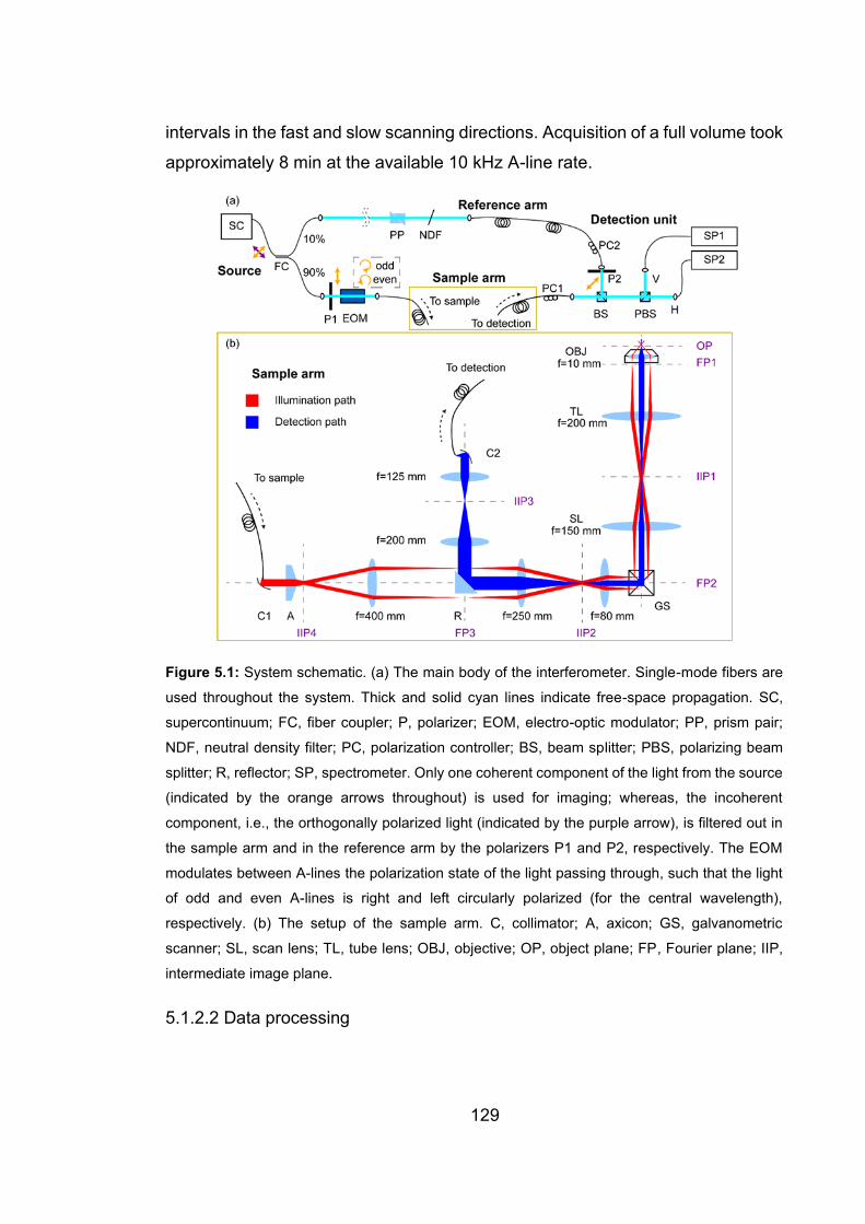
129
intervals in the fast and slow scanning directions. Acquisition of a full volume took
approximately 8 min at the available 10 kHz A-line rate.
Figure 5.1: System schematic. (a) The main body of the interferometer. Single-mode fibers are
used throughout the system. Thick and solid cyan lines indicate free-space propagation. SC,
supercontinuum; FC, fiber coupler; P, polarizer; EOM, electro-optic modulator; PP, prism pair;
NDF, neutral density filter; PC, polarization controller; BS, beam splitter; PBS, polarizing beam
splitter; R, reflector; SP, spectrometer. Only one coherent component of the light from the source
(indicated by the orange arrows throughout) is used for imaging; whereas, the incoherent
component, i.e., the orthogonally polarized light (indicated by the purple arrow), is filtered out in
the sample arm and in the reference arm by the polarizers P1 and P2, respectively. The EOM
modulates between A-lines the polarization state of the light passing through, such that the light
of odd and even A-lines is right and left circularly polarized (for the central wavelength),
respectively. (b) The setup of the sample arm. C, collimator; A, axicon; GS, galvanometric
scanner; SL, scan lens; TL, tube lens; OBJ, objective; OP, object plane; FP, Fourier plane; IIP,
intermediate image plane.
5.1.2.2 Data processing

130
A standard processing chain was used to reconstruct tomograms, including fixed
background removal, zeroing negative frequency content to recover the analytic
signal, interpolation from pixel to wavenumber domain, chromatic dispersion
compensation, spectral reshaping and apodization, Fourier transformation to z
domain, and relative sensitivity roll-off correction.
Careful relative alignment of the spectrometers’ pixel to wavenumber mapping
to match the spectral ranges is crucial for polarization-sensitive analysis [37]. We
first calibrated the two spectrometers individually, following the method of
Patarroyo et al. [38], which uses calibration measurements of a discrete sample
reflection at varying pathlength offsets to optimize both the mapping and the
dispersion imbalance. A difference in the spectral range results in diverging peak
positions in the tomograms of the two spectrometers; whereas, a relative spectral
offset causes a depth-dependent phase difference. Minimizing the position and
phase difference between the depth-varying calibration peak signals allowed
defining the pixel to wavenumber mapping of each spectrometer to ensure
matching spectral ranges. The calibration data also served to characterize and
compensate for relative depth-dependent signal roll-off between the two
spectrometers.
Tomograms were then combined to form Jones matrix tomograms, i.e., the
tomograms of the two detection channels of the same A-line define a Jones
vector and pairs of Jones vectors corresponding to illumination with orthogonal
polarization states determine the two columns of a Jones matrix. Polarization-
sensitive analysis of the Jones matrix tomograms was based on the formalism
presented in our recent work [28]. It compensates for wavelength-dependent
polarization distortions of the static system components and corrects for the effect
of preceding tissue layers to recover the depth-resolved, i.e., local, birefringence
and OA orientation. In brief, recovering the intrinsic transpose symmetry of the
Jones matrices served to compensate for system polarization distortions and
obtain corrected Jones matrix tomograms. The amplitude of the determinant of
the Jones matrix was used to define the structural image [39]. These Jones

131
matrices encode the cumulative polarization effect of the sample, which always
corresponds to the concurrent effect of a linear retarder and a linear diattenuator
when using identical illumination and detection paths [28]. The linear retardation
components of concurrently decomposed Jones matrices were converted to
SO(3) rotation matrices and spatially averaged by a 3D Gaussian kernel with an
isotropic full width at half maximum (FWHM) of 3 µm. Finally, local (i.e., depth-
resolved) linear SO(3) retardation matrices were recovered by recursive
correction for the effect of preceding tissue layers. The amount of rotation and
the angle of the rotation axis (by construction contained within the horizontal
plane of the Poincaré sphere) of the local SO(3) matrix correspond to the
retardation and the relative OA orientation of the local layer, respectively. The
relative axis orientation between the layers is accurately recovered, but there
remains an overall unknown offset in the axis orientation, which can be
determined by a priori knowledge of the sample in many instances.
Because the effective spectral bandwidth was approximately 8 times broader
than that of the conventional-resolution PS-OCT system previously used for
developing the processing method [28], which resulted in a larger k-dependence
of the system polarization distortions here, a few modifications of the correction
method were necessary. Firstly, 29 spectral bins instead of 15 were used to
estimate the correction matrices, with each bin extending over 12.5 % of the full
spectrum and adjacent bins overlapping with each other by 75 %. Secondly, the
retardation and the diattenuation vectors of the correction matrices were
smoothed with a linear filter corresponding to 7 % of the full spectral range, after
interpolation across different spectral bins to regularize the estimation of the
correction components over the full spectrum. Thirdly, to avoid a potential sign
ambiguity in the Jones matrix decomposition, the linear component of the system
transmission, as determined from the sample surface, was removed from the
cumulative sample Jones matrices.
All processing was performed with MATLAB R2016b on a workstation PC
equipped with an Intel CPU (i7-7700 @3.6GHz) and 32GB RAM. The total time

132
to process one full volumetric dataset (500 depth pixels × 3000 A-lines × 1500 B-
scans) was approximately 1 hour.
5.1.2.3 Sample preparation
Ocular tissues from freshly harvested adult sheep eye globes were scanned ex
vivo. Samples were obtained through institutional tissue sharing protocols from
unrelated projects that had been approved by the animal ethics committee of The
University of Western Australia. Eye globes were kept in Krebs solution. When
exposed to air before imaging, Krebs solution was applied to the samples to keep
them hydrated. All measurements were performed within 8 hours of harvesting.
5.1.3 Results
5.1.3.1 System performance and validation
First, we set out to validate the system design and characterize its performance.
The supercontinuum source, in combination with the wide-range spectrometers,
offered a measured axial resolution of 1.4 μm in air, corresponding to better than
1.0 μm in collagen-rich samples, assuming a refractive index of n = 1.45 [40]. The
focal properties of the decoupled illumination and detection modes are similar to
our previous OCM system used for ultrahigh-resolution optical coherence
elastography [31]. The annulus of the Bessel-like illumination path in the back
focal plane of the sample objective lens uses an effective numerical aperture of
NAeff = 0.26; whereas, the decoupled Gaussian detection mode corresponds to
NAeff = 0.14. Combined, they offered a lateral resolution (FWHM) of 1.6 µm,
extending over a DOF ~ 70 μ m, where DOF is defined as an axial OCM signal
roll-off ≤ 3 dB. Because the detection mode rejects specular reflections of the
Bessel-like illumination, system sensitivity cannot be directly measured by
evaluating the signal of an attenuated reflector. Instead, system sensitivity was
estimated to be > 100 dB with 7.0 mW of illumination power by comparing the
signal level in a scattering intralipid sample to that measured with a conventional
configuration using equal Gaussian illumination and detection modes, which, in
turn, allowed traditional evaluation of system sensitivity [30].
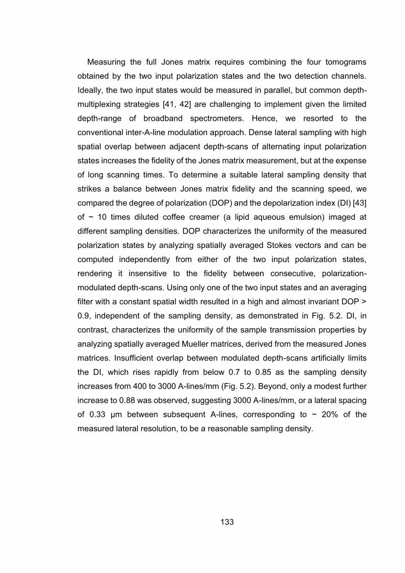
133
Measuring the full Jones matrix requires combining the four tomograms
obtained by the two input polarization states and the two detection channels.
Ideally, the two input states would be measured in parallel, but common depth-
multiplexing strategies [41, 42] are challenging to implement given the limited
depth-range of broadband spectrometers. Hence, we resorted to the
conventional inter-A-line modulation approach. Dense lateral sampling with high
spatial overlap between adjacent depth-scans of alternating input polarization
states increases the fidelity of the Jones matrix measurement, but at the expense
of long scanning times. To determine a suitable lateral sampling density that
strikes a balance between Jones matrix fidelity and the scanning speed, we
compared the degree of polarization (DOP) and the depolarization index (DI) [43]
of ~ 10 times diluted coffee creamer (a lipid aqueous emulsion) imaged at
different sampling densities. DOP characterizes the uniformity of the measured
polarization states by analyzing spatially averaged Stokes vectors and can be
computed independently from either of the two input polarization states,
rendering it insensitive to the fidelity between consecutive, polarization-
modulated depth-scans. Using only one of the two input states and an averaging
filter with a constant spatial width resulted in a high and almost invariant DOP >
0.9, independent of the sampling density, as demonstrated in Fig. 5.2. DI, in
contrast, characterizes the uniformity of the sample transmission properties by
analyzing spatially averaged Mueller matrices, derived from the measured Jones
matrices. Insufficient overlap between modulated depth-scans artificially limits
the DI, which rises rapidly from below 0.7 to 0.85 as the sampling density
increases from 400 to 3000 A-lines/mm (Fig. 5.2). Beyond, only a modest further
increase to 0.88 was observed, suggesting 3000 A-lines/mm, or a lateral spacing
of 0.33 μm between subsequent A-lines, corresponding to ~ 20% of the
measured lateral resolution, to be a reasonable sampling density.
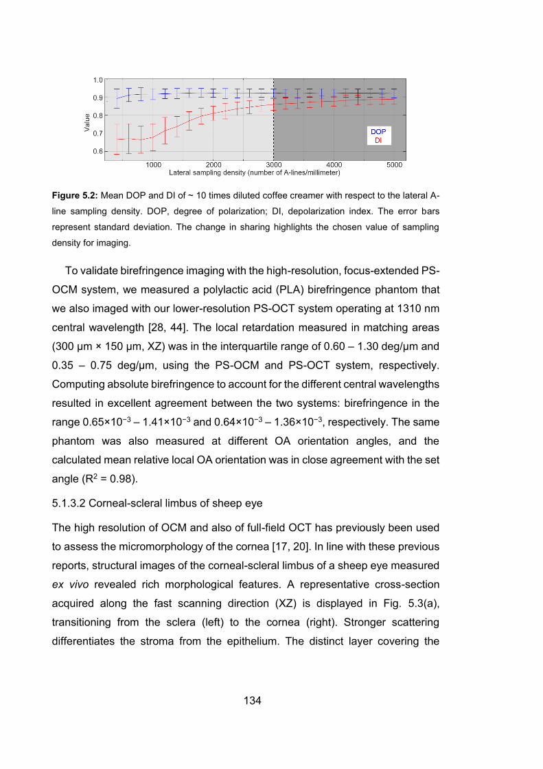
134
Figure 5.2: Mean DOP and DI of ~ 10 times diluted coffee creamer with respect to the lateral A-
line sampling density. DOP, degree of polarization; DI, depolarization index. The error bars
represent standard deviation. The change in sharing highlights the chosen value of sampling
density for imaging.
To validate birefringence imaging with the high-resolution, focus-extended PS-
OCM system, we measured a polylactic acid (PLA) birefringence phantom that
we also imaged with our lower-resolution PS-OCT system operating at 1310 nm
central wavelength [28, 44]. The local retardation measured in matching areas
(300 μm × 150 μm, XZ) was in the interquartile range of 0.60 ‒ 1.30 deg/μm and
0.35 ‒ 0.75 deg/μm, using the PS-OCM and PS-OCT system, respectively.
Computing absolute birefringence to account for the different central wavelengths
resulted in excellent agreement between the two systems: birefringence in the
range 0.65×10⁻³ ‒ 1.41×10⁻³ and 0.64×10⁻³ ‒ 1.36×10⁻³, respectively. The same
phantom was also measured at different OA orientation angles, and the
calculated mean relative local OA orientation was in close agreement with the set
angle (R2 = 0.98).
5.1.3.2 Corneal-scleral limbus of sheep eye
The high resolution of OCM and also of full-field OCT has previously been used
to assess the micromorphology of the cornea [17, 20]. In line with these previous
reports, structural images of the corneal-scleral limbus of a sheep eye measured
ex vivo revealed rich morphological features. A representative cross-section
acquired along the fast scanning direction (XZ) is displayed in Fig. 5.3(a),
transitioning from the sclera (left) to the cornea (right). Stronger scattering
differentiates the stroma from the epithelium. The distinct layer covering the
135
sclera is likely Tenon’s capsule, overlying the periscleral lymph space with
several vessels clearly visible. The stroma appears as a homogeneously
scattering body, interspersed only by stromal striae that present as vertically
oriented shadow-like structures [45]; three representative examples are marked
by the red asterisks in Fig. 5.3(a). Whilst high for OCT imaging, the achieved
spatial resolution is insufficient to reveal any detail on the internal organization of
the stroma. The lamellar architecture of the stroma, consisting of sheets or strips
of aligned collagen fibrils that have distinct, seemingly random orientations
parallel to the corneal surface, has been well established using microscopic
techniques, including PLM and SHG microscopy [46], but remains inaccessible
to OCT and OCM.
Figure 5.3(b) displays the local OA map corresponding to the same cross-
section using a 2D color map, encoding the local OA orientation in color and the
local retardation, after a further spatial filtering with a kernel of approximately
twice the size of the speckle, in brightness. The OA map reveals thin, clearly
defined, at times wavy, layers of distinct OA orientation that are entirely
indistinguishable in the structural intensity image. The local OA indicates the
angular direction of linear polarization, within the plane orthogonal to the
interrogating beam, that experiences the fastest propagation. In the case of
fibrillar collagen, this corresponds to the direction orthogonal to the fiber
orientation and suggests that consecutive layers have very distinct fiber
orientation, as expected from the individual lamellae. Because of the unknown
overall offset, it is possible, however, to treat the OA orientation as the fiber
orientation. On the left-hand side of the image in the sclera, layer thickness is
heterogeneous, with some very thin layers sandwiched between thicker layers.
In the cornea on the right-hand side, the layers appear uniformly thin.
Interestingly, the striae, while clearly visible in the scattering signal, have little
impact on the OA signal and are invisible in the OA maps. Reconstructing the
local OA corrects for the cumulative polarization rotating effect of preceding
layers, but there remains an overall unknown orientation offset, leaving the
absolute 0˚ direction undefined. Also, depth-correction is only possible with

136
sufficient signal and areas with low SNR (< 7 dB in the stroma and < 15 dB in the
epithelium) are, thus, grayed out. Furthermore, the OA is only meaningful in areas
with sufficient local retardation. Indeed, where not masked, the OA orientation in
the epithelium and other tissue ahead of the stroma appears random, with two
dominating apparent OA orientations encoded in green and purple, respectively,
but without defining layers of continuous OA orientation. A fly-through video of
the micro-morphology and the local OA orientation of the entire volume (1 mm ×
1 mm × 0.45 mm, XYZ) is available as Visualization 5.1.
Figure 5.3: A representative cross-sectional view (in the fast scanning direction, XZ) of the
intensity (a), local OA orientation (b), local retardation (c), and DI (d), of the corneal-sclera limbus
region of an adult sheep eye globe (Sample #1), imaged ex vivo. Epi, epithelium; OA, optic axis;
DI, depolarization index. The local OA orientation image is color coded and overlaid with the local
retardation as brightness, as indicted by the color bar and wheel in panel (b). The red asterisks
in (a) indicate three representative stromal striae. The dashed cyan lines in (a) and (b) correspond
to the cross-sections in the slow scanning direction (YZ), shown in Fig. 5.4. The white arrow in

137
(b) and the white arrow in Fig. 5.4(a) highlight the same OA layer in orthogonal cross-sections.
The black arrow in (d) indicates the high depolarizing layer, presumed to be Tenon’s capsule. A
fly-through video of the volumetric data (1.0 mm × 1.0 mm × 0.45 mm, XYZ) is available as
Visualization 5.1. Scale bars: 100 μm.
Figure 5.3(c) shows the local retardation, overlaid with the intensity image as
brightness. Whilst the range of local retardation values is high for biological
samples, the local retardation image exhibits only poor contrast and does not
reveal any clear features. Figure 5.3(d) displays the DI, in a similar overlay with
the intensity image. As well as an obvious noise-induced depolarization
noticeable at deeper sample locations, Tenon’s capsule induces pronounced
depolarization, indicated by the black arrow in (d).
To further illustrate the change in thickness of the observed layers between
the sclera and the cornea, Fig. 5.4 presents cross-sectional views of the same
volumetric data along the slow scanning direction (YZ), taken at the positions of
the dashed cyan lines in Figs. 5.3(a) and (b), respectively. A fly-through video of
the volumetric data (1 mm × 1 mm × 0.45 mm, XYZ) in this orientation is available
as Visualization 5.2, highlighting the smooth transition in layer thickness from the
sclera to the cornea. Leveraging the distinct advantage of volumetric imaging
over histology, we point out one interesting fiber bundle, i.e., the yellow layer
marked by the white arrow in Fig. 5.3(b) and Fig. 5.4(a). It extends over almost
500 µm of the trans-ocular cross-section in Fig. 5.3(b) but has a shorter width of
approximately 200 μm in Fig. 5.4(a), suggesting a radial orientation of this
particular strip. From this observation, it can be inferred that the yellow color in
the local OA orientation points to the center of the cornea; whereas, the blue color
is orthogonal, i.e., in the azimuthal direction.
138
Figure 5.4: Three representative cross-sectional views (in the slow scanning direction, YZ) of the
intensity (left column) and local OA orientation (right column) of Sample #1. (a-c) are from the
sclera, limbus and cornea, respectively, corresponding to the dashed cyan lines in Figs. 5.3(a)
and (b), from left to right. The dashed red lines correspond to the cross-section in Fig. 5.3. The
white arrow and dashed ellipse in (a) and the white arrow in Fig. 5.3(b) highlight the same OA
layer in orthogonal cross-sections. Epi, epithelium. A fly-through video of the volumetric data (1
mm × 1 mm × 0.45 mm, XYZ) is available as Visualization 5.2. Scale bars: 100 μm.
A representative cross-sectional view of the intensity and the local OA
orientation of the limbus region imaged in a second sample is presented in Fig.
5.5. In this sample, the individual layers in the stroma form more complex
networks than observed in the first sample, suggesting possible fusing and
branching [1]. Again, nothing in the structural images discloses this intricate
internal organization that is only revealed by the local OA image, and best
appreciated in the fly-through video of the volumetric data (1 mm × 0.5 mm × 0.54
mm, XYZ), available as Visualization 5.3.
Overall, conventional backscatter tomograms and local retardation images
(not shown) of the stromal tissue in the limbus region of sheep eyes provide
valuable image contrast but do not reveal the detailed tissue organization related
to the directional arrangement of fibrillar tissue components. In comparison, the
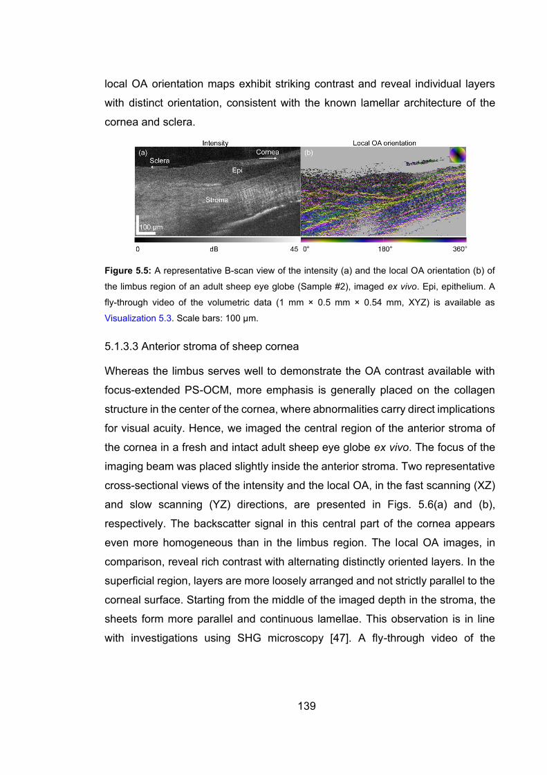
139
local OA orientation maps exhibit striking contrast and reveal individual layers
with distinct orientation, consistent with the known lamellar architecture of the
cornea and sclera.
Figure 5.5: A representative B-scan view of the intensity (a) and the local OA orientation (b) of
the limbus region of an adult sheep eye globe (Sample #2), imaged ex vivo. Epi, epithelium. A
fly-through video of the volumetric data (1 mm × 0.5 mm × 0.54 mm, XYZ) is available as
Visualization 5.3. Scale bars: 100 μm.
5.1.3.3 Anterior stroma of sheep cornea
Whereas the limbus serves well to demonstrate the OA contrast available with
focus-extended PS-OCM, more emphasis is generally placed on the collagen
structure in the center of the cornea, where abnormalities carry direct implications
for visual acuity. Hence, we imaged the central region of the anterior stroma of
the cornea in a fresh and intact adult sheep eye globe ex vivo. The focus of the
imaging beam was placed slightly inside the anterior stroma. Two representative
cross-sectional views of the intensity and the local OA, in the fast scanning (XZ)
and slow scanning (YZ) directions, are presented in Figs. 5.6(a) and (b),
respectively. The backscatter signal in this central part of the cornea appears
even more homogeneous than in the limbus region. The local OA images, in
comparison, reveal rich contrast with alternating distinctly oriented layers. In the
superficial region, layers are more loosely arranged and not strictly parallel to the
corneal surface. Starting from the middle of the imaged depth in the stroma, the
sheets form more parallel and continuous lamellae. This observation is in line
with investigations using SHG microscopy [47]. A fly-through video of the
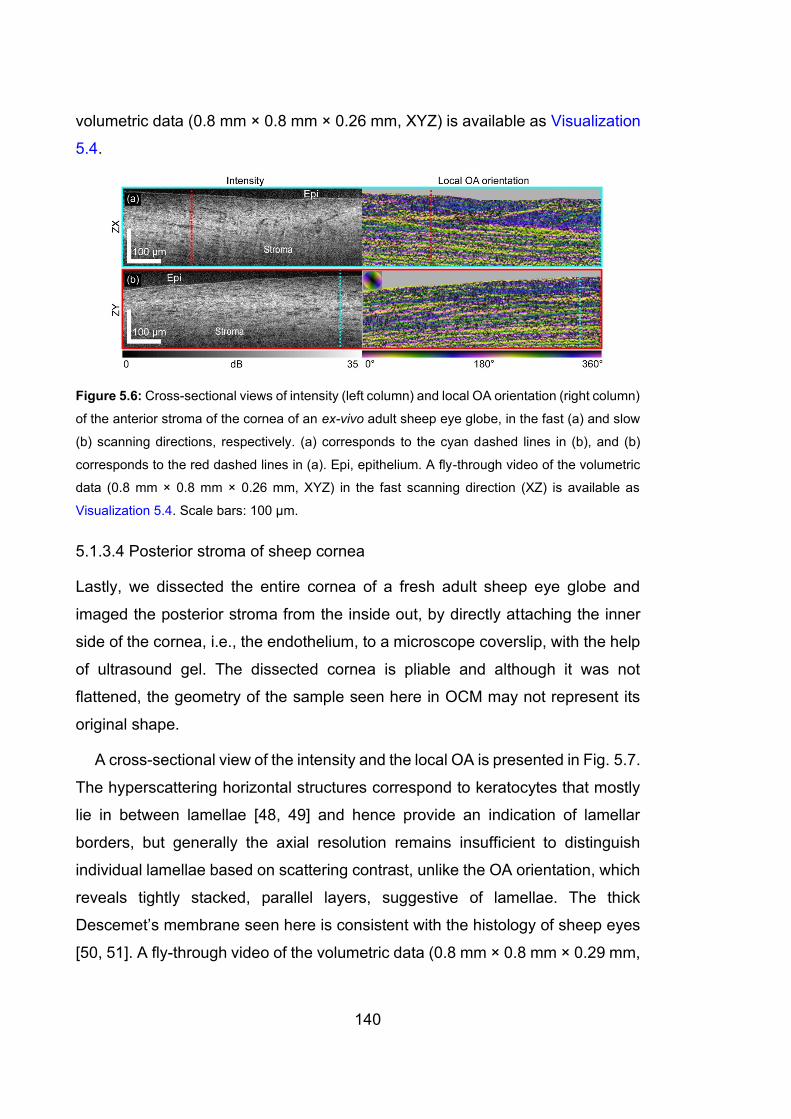
140
volumetric data (0.8 mm × 0.8 mm × 0.26 mm, XYZ) is available as Visualization
5.4.
Figure 5.6: Cross-sectional views of intensity (left column) and local OA orientation (right column)
of the anterior stroma of the cornea of an ex-vivo adult sheep eye globe, in the fast (a) and slow
(b) scanning directions, respectively. (a) corresponds to the cyan dashed lines in (b), and (b)
corresponds to the red dashed lines in (a). Epi, epithelium. A fly-through video of the volumetric
data (0.8 mm × 0.8 mm × 0.26 mm, XYZ) in the fast scanning direction (XZ) is available as
Visualization 5.4. Scale bars: 100 μm.
5.1.3.4 Posterior stroma of sheep cornea
Lastly, we dissected the entire cornea of a fresh adult sheep eye globe and
imaged the posterior stroma from the inside out, by directly attaching the inner
side of the cornea, i.e., the endothelium, to a microscope coverslip, with the help
of ultrasound gel. The dissected cornea is pliable and although it was not
flattened, the geometry of the sample seen here in OCM may not represent its
original shape.
A cross-sectional view of the intensity and the local OA is presented in Fig. 5.7.
The hyperscattering horizontal structures correspond to keratocytes that mostly
lie in between lamellae [48, 49] and hence provide an indication of lamellar
borders, but generally the axial resolution remains insufficient to distinguish
individual lamellae based on scattering contrast, unlike the OA orientation, which
reveals tightly stacked, parallel layers, suggestive of lamellae. The thick
Descemet’s membrane seen here is consistent with the histology of sheep eyes
[50, 51]. A fly-through video of the volumetric data (0.8 mm × 0.8 mm × 0.29 mm,
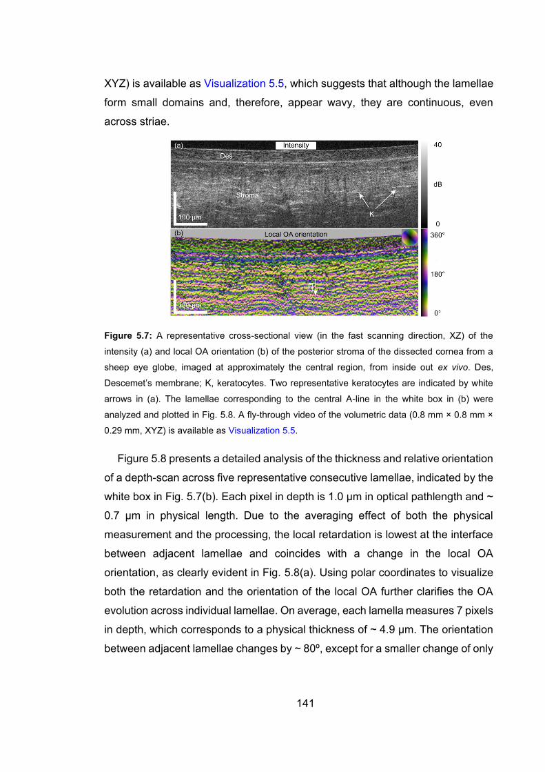
141
XYZ) is available as Visualization 5.5, which suggests that although the lamellae
form small domains and, therefore, appear wavy, they are continuous, even
across striae.
Figure 5.7: A representative cross-sectional view (in the fast scanning direction, XZ) of the
intensity (a) and local OA orientation (b) of the posterior stroma of the dissected cornea from a
sheep eye globe, imaged at approximately the central region, from inside out ex vivo. Des,
Descemet’s membrane; K, keratocytes. Two representative keratocytes are indicated by white
arrows in (a). The lamellae corresponding to the central A-line in the white box in (b) were
analyzed and plotted in Fig. 5.8. A fly-through video of the volumetric data (0.8 mm × 0.8 mm ×
0.29 mm, XYZ) is available as Visualization 5.5.
Figure 5.8 presents a detailed analysis of the thickness and relative orientation
of a depth-scan across five representative consecutive lamellae, indicated by the
white box in Fig. 5.7(b). Each pixel in depth is 1.0 μm in optical pathlength and ~
0.7 μm in physical length. Due to the averaging effect of both the physical
measurement and the processing, the local retardation is lowest at the interface
between adjacent lamellae and coincides with a change in the local OA
orientation, as clearly evident in Fig. 5.8(a). Using polar coordinates to visualize
both the retardation and the orientation of the local OA further clarifies the OA
evolution across individual lamellae. On average, each lamella measures 7 pixels
in depth, which corresponds to a physical thickness of ~ 4.9 μm. The orientation
between adjacent lamellae changes by ~ 80º, except for a smaller change of only

142
~ 60º between the 3rd and the 4th layer. We conclude that adjacent lamellae
have random orientation relative to each other, in agreement with observations
using SHG microscopy [11, 52].
Figure 5.8: A quantitative analysis of local OA orientation and local retardation in five
representative lamellae in the posterior stroma. (a) Plot of the local OA orientation and the local
retardation in a short segment of a representative A-line, located in the center of the white box in
Fig. 5.7(b). Five lamellae are distinguished in this range. OPL, optical path length. (b),(c) Plots of
the vectorized local OA orientation and local retardation of the five lamellae in polar coordinates,
where the local OA orientation and local retardation are represented as the angle and the length
of the vectors, respectively. In (b) and (c), the radius of the semicircles represents 4.0 deg/μm of
local retardation.
5.1.4 Discussion
This study demonstrates the striking contrast of local OA imaging when combined
with the improved spatial resolution of OCM. Depending on the specific tissue
morphology, scattering contrast may be sufficient to reveal relevant details at high
spatial resolution, as in the coronary arteries [53] or for imaging of Alzheimer’s
plaques [54]. In the cornea, OCM resolves fine details including nerves,
keratocytes, and stromal striae, but detecting the orientation of collagen fibers
and inspecting their microscopic arrangement remains difficult simply based on
spatially resolved measurements of the amplitude of backscattered light.
143
However, the orientation of collagen fibers induces minute polarization-
dependent phase differences in the backscattered light, which we utilize to
reconstruct the local OA orientation from polarization-sensitive measurements.
As evidenced with focus-extended PS-OCM images of the limbus and cornea,
local OA images offer an impressive contrast between adjacent tissue layers that
only differ in their orientation and are indistinguishable in structural tomograms.
Similarly, the scalar amount of local retardation proved difficult to interpret, likely
because the layers feature comparable local retardation and only contrast in their
OA orientation. Previous measurements of human sclera with lower resolution in
the 1.3 µm wavelength region have resulted in much lower local retardation
values (<1 deg/µm) [55], even when considering the difference in wavelength.
Our higher retardation values (~ 3 deg/µm) are likely the result of the improved
spatial resolution, which reduces the extent of averaging across several
differently oriented collagen fibers.
To the best of our knowledge, this work is the first demonstration of high-
resolution local OA imaging. Previous efforts combining PS-OCT with the high
resolution of OCM used cumulative OA imaging of brain tissue [56, 57]. The
correction for system polarization distortions and the reconstruction of the local
instead of the cumulative OA orientation employed in the current work were
critical to obtain the presented results. The polarization states across the wide
wavelength range required to achieve high axial resolution are bound to
experience spectrally dependent variations upon propagation through the system
components, leading to artifacts in the reconstructed OA and birefringence maps.
Indeed, in conventional retinal PS-OCT, the transmission through the cornea
only imparts a modest polarization change on the imaging beam that can be
compensated [58]. Direct investigation of the cumulative retardation and OA of
the cornea exhibits characteristic patterns exceeding a quarter-wave of
retardation and has been shown to differ in keratoconus patients [59]. The extent
to which the angle of incidence on the corneal surface impacts the observed
retardation effects remains a topic of investigation [60]. On the macroscopic scale,

144
the cumulative retardation across the full thickness of the cornea, consisting of a
stack of thin lamellae with random orientations, can be expected to be modest.
Although each lamella exhibits moderate birefringence, an adjacent lamella with
an OA oriented at 90˚ entirely compensates the retardation across the pair of
lamellae. The more random angular orientation reported from mammalian
corneas [52] still results, overall, in the absence of any pronounced retardation.
However, inspecting the corneal polarization properties with the improved spatial
resolution of our focus-extended PS-OCM displays a dramatically different
picture. The observed OA patterns of distinctly oriented layers closely match the
expected organization of stromal tissue into tightly stacked lamellae. The
estimated layer thickness of ~ 4.9 µm is consistent with reports of transmission
electron microscopy of adult sheep cornea [51], although literature values for
lamellar thickness in human cornea are smaller [61]. Currently, our results lack
comparison with histopathology confirming a direct association of the observed
OA layers with individual lamellae. Future studies are needed to examine if the
resolution of focus-extended PS-OCM is sufficient to resolve lamellae in human
cornea.
A further limitation of our work is the investigation of excised eye globes ex
vivo. Previous studies of PS-OCT in the cornea suggested specific depolarization
signatures only arise in vivo [60]. It remains an open question if and how this
would impact local OA imaging. There is no fundamental barrier to performing
focus-extended PS-OCM in vivo. In this initial investigation of combining local OA
imaging with OCM, the high relative intensity noise of the available
supercontinuum source limited the acquisition speed. Newer sources with higher
pump repetition rates have been shown to allow OCT operation with a 70 kHz A-
line rate in the shot-noise limit [62]. Depth-encoding the two input polarization
states instead of sequential modulation would relieve the tight spatial sampling
constraint and enable faster and more flexible scanning. The implemented focus
scheme already ensures that a tight lateral resolution can be maintained over an
extended axial range and avoids the multiple acquisitions with varied axial focus
positions of conventional OCM [63, 64]. Although the nominal DOF, defined as
145
the FWHM of the product of the intensity profiles of the illuminating Bessel beam
and the detecting Gaussian beam, is only approximately 70 μm, the practical
imaging range providing meaningful intensity images and OA orientation maps
extends well beyond 300 µm. The long tail of the Bessel-like illumination results
in a slow decay of the illumination power behind the focus position, maintaining
an appreciable signal beyond the nominal DOF. In the intensity images, the
logarithmic display helps to produce an appreciable gray-level at these depth
positions. The OA maps depend primarily on the SNR, and hence benefit from
the same extended range. Combination with numerical refocusing may enable
imaging through the entire cornea, since it would potentially enable one to correct
for aberrations that limit the imaging depth in tissue achievable at high resolution
[65].
There remains room for improving the local OA reconstruction method.
Currently, the compensation for the preceding tissue layers occurs recursively,
starting from the sample surface. When focusing deeper inside a sample, the
surface signal may have limited SNR and only provide a poor starting point for
this correction. In these situations, we started from a higher SNR area within the
sample but lost the surface reference that would be needed when attempting to
convert the relative to absolute OA orientations. Also, the processing assumes
that polarization-dependent scattering amplitude, i.e., diattenuation, is negligible
and casts the measurements into the SO(3) formalism. Whilst static system
diattenuation is corrected by our processing before conversion to the SO(3)
formalism, we found that its presence makes the noise polarization-dependent,
and causes preferential OA directions in noise-dominated regions with low
birefringence. This explains the observed OA pattern in the epithelium and the
Descemet’s membrane, which are both cellular and not fibrillar structures. A more
rigorous strategy to treat system diattenuation and consider sample diattenuation
and depolarization effects may achieve improved results and reveal additional
sample features.
146
We highlighted the remarkable opportunities for high-resolution OA imaging
by inspecting structures in the anterior eye. Such imaging could be of particular
interest for the study and diagnosis of keratoconus, which involves alterations in
the collagen lamellae and fibrils [66, 67], leading to a loss of the normal
interwoven structure of the lamellae [68, 69]. Whereas current diagnostic
strategies, including Brillouin microscopy [14], probe the biomechanical
properties of the thinning cornea, OA imaging may offer direct insight into the
altered collagen morphology. Besides the anterior eye, there are numerous
tissues with similarly intricate fibrillar architectures. Further progress in local OA
imaging, in combination with the high spatial resolution of OCM, may enable the
investigation of the skin, nerves, vessel walls, or cartilage in vivo on the
microscopic scale, which remains difficult to date.
5.1.5 Conclusions
Vectorial birefringence enables detailed study of the organization of intact fibrillar
tissues, probing tissue organization on length scales beyond the imaging
resolution. Our results demonstrate that the improved spatial resolution of focus-
extended PS-OCM is critical to avoid averaging of the birefringence features and
to resolve relevant morphological features. Whereas tomograms of the
backscatter-intensity and the scalar amount of local birefringence failed to reliably
differentiate individual lamellar layers in sheep cornea, the local OA orientation
reveals distinct layers with striking contrast, suggesting that the vectorial property
of birefringence is more resilient to the detrimental averaging effects of limited
spatial resolution. The same contrast enhancement may enable human in vivo
imaging, with suitable improvements in the imaging speed, for investigation of the
cornea or other organs accessible to OCM imaging.
Funding
Australian Research Council (DP160104969); National Institutes of Health
(P41EB-015903 and R03EB-024803); Western Australian Department of Health
Merit Award and the Medical and Health Research Infrastructure Fund.
147
Acknowledgements
The authors acknowledge Dr. Andrea Curatolo, Dr. Danuta Sampson, Prof. Dao-
Yi Yu, Dr. Peijun Gong, Dr. Nishant Mohan, Prof. Chulmin Joo and Dr. Boy Braaf
for fruitful discussions. Q. Li acknowledges the financial support of the Australian
Government International Research Training Program (RTP) Fee Offset
Scholarships.
Disclosures
The authors declare that there are no conflicts of interest related to this article.
References for Section 5.1
1. K. M. Meek and C. Knupp, "Corneal structure and transparency," Prog. Retin.
Eye Res. 49, 1‒16 (2015).
2. S. Yamamoto, H. Hashizume, J. Hitomi, M. Shigeno, S. Sawaguchi, H. Abe,
and T. Ushiki, "The subfibrillar arrangement of corneal and scleral collagen
fibrils as revealed by scanning electron and atomic force microscopy," Arch.
Histol. Cytol. 63(2), 127‒135 (2000).
3. W. Radner, M. Zehetmayer, R. Aufreiter, and R. Mallinger, "Interlacing and
cross-angle distribution of collagen lamellae in the human cornea," Cornea
17(5), 537‒543 (1998).
4. K. M. Meek and C. Boote, "The use of X-ray scattering techniques to quantify
the orientation and distribution of collagen in the corneal stroma," Prog. Retin
Eye Res. 28(5), 369‒392 (2009).
5. K. M. Meek and A. J. Quantock, "The use of X-ray scattering techniques to
determine corneal ultrastructure," Prog. Retin Eye Res. 20(1), 95‒137 (2001).
6. N.-J. Jan, J. L. Grimm, H. Tran, K. L. Lathrop, G. Wollstein, R. A. Bilonick, H.
Ishikawa, L. Kagemann, J. S. Schuman, and I. A. Sigal, "Polarization
microscopy for characterizing fiber orientation of ocular tissues," Biomed. Opt.
Express 6(12), 4705‒4718 (2015).

148
7. N.-J. Jan, B. L. Brazile, D. Hu, G. Grube, J. Wallace, A. Gogola, and I. A. Sigal,
"Crimp around the globe; patterns of collagen crimp across the corneoscleral
shell," Exp. Eye Res. 172, 159‒170 (2018).
8. B. Yang, N.-J. Jan, B. Brazile, A. Voorhees, K. L. Lathrop, and I. A. Sigal,
"Polarized light microscopy for 3-dimensional mapping of collagen fiber
architecture in ocular tissues," J. Biophotonics 11, e201700356 (2018).
9. Y. Mega, M. Robitaille, R. Zareian, J. McLean, J. Ruberti, and C. DiMarzio,
"Quantification of lamellar orientation in corneal collagen using second
harmonic generation images," Opt. Lett. 37(16), 3312‒3314 (2012).
10. S.-W. Teng, H.-Y. Tan, J.-L. Peng, H.-H. Lin, K. H. Kim, W. Lo, Y. Sun, W.-C.
Lin, S.-J. Lin, S.-H. Jee, P. T. C. So, and C.-Y. Dong, "Multiphoton
autofluorescence and second-harmonic generation imaging of the ex vivo
porcine eye," Invest. Ophthalmol. Vis. Sci. 47(3), 1216‒1224 (2006).
11.G. Latour, I. Gusachenko, L. Kowalczuk, I. Lamarre, and M.-C. Schanne-Klein,
"In vivo structural imaging of the cornea by polarization-resolved second
harmonic microscopy," Biomed. Opt. Express 3(1), 1‒15 (2012).
12. G. Scarcelli and S. H. Yun, "In vivo Brillouin optical microscopy of the human
eye," Opt. Express 20(8), 9197‒9202 (2012).
13. G. Scarcelli and S. H. Yun, "Confocal Brillouin microscopy for three-
dimensional mechanical imaging," Nat. Photonics 2(1), 39‒43 (2008).
14. T. G. Seiler, P. Shao, A. Eltony, T. Seiler, and S.-H. Yun, "Brillouin
spectroscopy of normal and keratoconus corneas," Am. J. Ophthalmol. 202,
118‒125 (2019).
15. M. Ang, M. Baskaran, R. M. Werkmeister, J. Chua, D. Schmidl, V. Aranha dos
Santos, G. Garhöfer, J. S. Mehta, and L. Schmetterer, "Anterior segment
optical coherence tomography," Prog. Retin. Eye Res. 66, 132‒156 (2018).
149
16. J. L. B. Ramos, Y. Li, and D. Huang, "Clinical and research applications of
anterior segment optical coherence tomography – a review," Clin. Experiment.
Ophthalmol. 37(1), 81‒89 (2009).
17. R. M. Werkmeister, S. Sapeta, D. Schmidl, G. Garhöfer, G. Schmidinger, V.
Aranha dos Santos, G. C. Aschinger, I. Baumgartner, N. Pircher, F.
Schwarzhans, A. Pantalon, H. Dua, and L. Schmetterer, "Ultrahigh-resolution
OCT imaging of the human cornea," Biomed. Opt. Express 8(2), 1221‒1239
(2017).
18. K. Bizheva, B. Tan, B. MacLelan, O. Kralj, M. Hajialamdari, D. Hileeto, and L.
Sorbara, "Sub-micrometer axial resolution OCT for in-vivo imaging of the
cellular structure of healthy and keratoconic human corneas," Biomed. Opt.
Express 8(2), 800‒812 (2017).
19. B. Tan, Z. Hosseinaee, L. Han, O. Kralj, L. Sorbara, and K. Bizheva, "250 kHz,
1.5 µm resolution SD-OCT for in-vivo cellular imaging of the human cornea,"
Biomed. Opt. Express 9(12), 6569‒6583 (2018).
20. V. Mazlin, P. Xiao, E. Dalimier, K. Grieve, K. Irsch, J.-A. Sahel, M. Fink, and
A. C. Boccara, "In vivo high resolution human corneal imaging using full-field
optical coherence tomography," Biomed. Opt. Express 9(2), 557‒568 (2018).
21. R. Oldenbourg, "A new view on polarization microscopy," Nature 381(6585),
811 (1996).
22. R. A. Carlton, "Polarized Light Microscopy," in Pharmaceutical Microscopy, R.
A. Carlton, ed. (Springer New York, New York, NY, 2011), pp. 7‒64.
23. J. F. de Boer, C. K. Hitzenberger, and Y. Yasuno, "Polarization sensitive
optical coherence tomography - a review [Invited]," Biomed. Opt. Express 8(3),
1838‒1873 (2017).
24. B. Baumann, "Polarization sensitive optical coherence tomography: A review
of technology and applications," Appl. Sci. 7(5), 474 (2017).

150
25. C. Fan and G. Yao, "Mapping local optical axis in birefringent samples using
polarization-sensitive optical coherence tomography," J. Biomed. Opt. 17(11),
110501 (2012).
26. C. Fan and G. Yao, "Imaging myocardial fiber orientation using polarization
sensitive optical coherence tomography," Biomed. Opt. Express 4(3), 460‒
465 (2013).
27. M. Villiger, B. Braaf, N. Lippok, K. Otsuka, S. K. Nadkarni, and B. E. Bouma,
"Optic axis mapping with catheter-based polarization-sensitive optical
coherence tomography," Optica 5(10), 1329‒1337 (2018).
28. Q. Li, K. Karnowski, P. B. Noble, A. Cairncross, A. James, M. Villiger, and D.
D. Sampson, "Robust reconstruction of local optic axis orientation with fiber-
based polarization-sensitive optical coherence tomography," Biomed. Opt.
Express 9(11), 5437‒5455 (2018).
29. R. A. Leitgeb, M. Villiger, A. H. Bachmann, L. Steinmann, and T. Lasser,
"Extended focus depth for Fourier domain optical coherence microscopy," Opt.
Lett. 31(16), 2450‒2452 (2006).
30. M. Villiger, C. Pache, and T. Lasser, "Dark-field optical coherence
microscopy," Opt. Lett. 35(20), 3489‒3491 (2010).
31. A. Curatolo, M. Villiger, D. Lorenser, P. Wijesinghe, A. Fritz, B. F. Kennedy,
and D. D. Sampson, "Ultrahigh-resolution optical coherence elastography,"
Opt. Lett. 41(1), 21‒24 (2016).
32. C. E. Saxer, J. F. de Boer, B. H. Park, Y. Zhao, Z. Chen, and J. S. Nelson,
"High-speed fiber-based polarization-sensitive optical coherence tomography
of in vivo human skin," Opt. Lett. 25(18), 1355‒1357 (2000).
33. B. H. Park, M. C. Pierce, B. Cense, and J. F. de Boer, "Real-time multi-
functional optical coherence tomography," Opt. Express 11(7), 782‒793
(2003).
151
34. D. Lorenser, C. Christian Singe, A. Curatolo, and D. D. Sampson, "Energy-
efficient low-Fresnel-number Bessel beams and their application in optical
coherence tomography," Opt. Lett. 39(3), 548‒551 (2014).
35. M. Wojtkowski, V. J. Srinivasan, T. H. Ko, J. G. Fujimoto, A. Kowalczyk, and
J. S. Duker, "Ultrahigh-resolution, high-speed, Fourier domain optical
coherence tomography and methods for dispersion compensation," Opt.
Express 12(11), 2404‒2422 (2004).
36. J. F. de Boer, R. Leitgeb, and M. Wojtkowski, "Twenty-five years of optical
coherence tomography: the paradigm shift in sensitivity and speed provided
by Fourier domain OCT [Invited]," Biomed. Opt. Express 8(7), 3248‒3280
(2017).
37. M. Mujat, B. H. Park, B. Cense, T. C. Chen, and J. F. de. Boer,
"Autocalibration of spectral-domain optical coherence tomography
spectrometers for in vivo quantitative retinal nerve fiber layer birefringence
determination," J. Biomed. Opt. 12(4), 041205 (2007).
38. N. Uribe-Patarroyo, S. H. Kassani, M. Villiger, and B. E. Bouma, "Robust
wavenumber and dispersion calibration for Fourier-domain optical coherence
tomography," Opt. Express 26(7), 9081‒9094 (2018).
39. J. Li and J. F. de Boer, "Coherent signal composition and global phase
determination in signal multiplexed polarization sensitive optical coherence
tomography," Opt. Express 22(18), 21382‒21392 (2014).
40. A. N. Bashkatov, E. A. Genina, V. I. Kochubey, and V. V. Tuchin, "Estimation
of wavelength dependence of refractive index of collagen fibers of scleral
tissue," Proc. SPIE 4162, 265‒268 (2000).
41. B. Baumann, W. Choi, B. Potsaid, D. Huang, J. S. Duker, and J. G. Fujimoto,
"Swept source/Fourier domain polarization sensitive optical coherence
tomography with a passive polarization delay unit," Opt. Express 20(9),
10229‒10241 (2012).

152
42. Y. Lim, Y.-J. Hong, L. Duan, M. Yamanari, and Y. Yasuno, "Passive
component based multifunctional Jones matrix swept source optical
coherence tomography for Doppler and polarization imaging," Opt. Lett.
37(11), 1958‒1960 (2012).
43. N. Lippok, M. Villiger, and B. E. Bouma, "Degree of polarization (uniformity)
and depolarization index: unambiguous depolarization contrast for optical
coherence tomography," Opt. Lett. 40(17), 3954‒3957 (2015).
44. J. Walther, Q. Li, M. Villiger, C. S. Farah, E. Koch, K. Karnowski, and D. D.
Sampson, "Depth-resolved birefringence imaging of collagen fiber
organization in the human oral mucosa in vivo," Biomed. Opt. Express 10(4),
1942‒1956 (2019).
45. K. Grieve, D. Ghoubay, C. Georgeon, G. Latour, A. Nahas, K. Plamann, C.
Crotti, R. Bocheux, M. Borderie, T.-M. Nguyen, F. Andreiuolo, M.-C. Schanne-
Klein, and V. Borderie, "Stromal striae: a new insight into corneal physiology
and mechanics," Sci. Rep. 7(1), 13584 (2017).
46. M. Winkler, D. Chai, S. Kriling, C. J. Nien, D. J. Brown, B. Jester, T. Juhasz,
and J. V. Jester, "Nonlinear optical macroscopic assessment of 3-D corneal
collagen organization and axial biomechanics," Invest. Ophthamol. Vis. Sci.
52(12), 8818‒8827 (2011).
47. N. Morishige, Y. Takagi, T.-i. Chikama, A. Takahara, and T. Nishida, "Three-
dimensional analysis of collagen lamellae in the anterior stroma of the human
cornea visualized by second harmonic generation imaging microscopy,"
Invest. Ophthalmol. Vis. Sci. 52(2), 911‒915 (2011).
48. J. A. West-Mays and D. J. Dwivedi, "The keratocyte: Corneal stromal cell with
variable repair phenotypes," Int. J. Biochemi. Cell Biol. 38(10), 1625‒1631
(2006).
49. G. H.-F. Yam, G. P. Williams, M. Setiawan, N. Z. B. M. Yusoff, X.-w. Lee, H.
M. Htoon, L. Zhou, M. Fuest, and J. S. Mehta, "Nerve regeneration by human
153
corneal stromal keratocytes and stromal fibroblasts," Sci. Rep. 7(1), 45396
(2017).
50. C. A. Greene, S. L. Misra, H. Lee, J. McKelvie, K. Kapadia, R. McFarlane, C.
N. J. McGhee, C. R. Green, and T. Sherwin, "The sheep cornea: structural
and clinical characteristics," Curr. Eye Res. 43(12), 1432‒1438 (2018).
51. T. A. Cafaro, M. F. Suarez, C. Maldonado, J. O. Croxatto, C. Insfrán, J. A.
Urrets-Zavalía, and H. M. Serra, "On the cornea of healthy merino sheep: a
detailed ex vivo confocal, histological and ultrastructural study," Anat. Histol.
Embryol. 44(4), 247‒254 (2015).
52. M. Winkler, G. Shoa, S. T. Tran, Y. Xie, S. Thomasy, V. K. Raghunathan, C.
Murphy, D. J. Brown, and J. V. Jester, "A comparative study of vertebrate
corneal structure: The evolution of a refractive lensvertebrate corneal
structure," Invest. Ophthalmol. Vis. Sci. 56(4), 2764‒2772 (2015).
53. L. Liu, J. A. Gardecki, S. K. Nadkarni, J. D. Toussaint, Y. Yagi, B. E. Bouma,
and G. J. Tearney, "Imaging the subcellular structure of human coronary
atherosclerosis using micro-optical coherence tomography," Nat. Med. 17(8),
1010‒1014 (2011).
54. T. Bolmont, A. Bouwens, C. Pache, M. Dimitrov, C. Berclaz, M. Villiger, B. M.
Wegenast-Braun, T. Lasser, and P. C. Fraering, "Label-free imaging of
cerebral β-amyloidosis with extended-focus optical coherence microscopy," J.
Neurosci. 32(42), 14548‒14556 (2012).
55. M. Yamanari, S. Nagase, S. Fukuda, K. Ishii, R. Tanaka, T. Yasui, T. Oshika,
M. Miura, and Y. Yasuno, "Scleral birefringence as measured by polarization-
sensitive optical coherence tomography and ocular biometric parameters of
human eyes in vivo," Biomed. Opt. Express 5(5), 1391‒1402 (2014).
56. H. Wang, T. Akkin, C. Magnain, R. Wang, J. Dubb, W. J. Kostis, M. A. Yaseen,
A. Cramer, S. Sakadžić, and D. Boas, "Polarization sensitive optical
coherence microscopy for brain imaging," Opt. Lett. 41(10), 2213‒2216
(2016).
154
57. B. Baumann, A. Woehrer, G. Ricken, M. Augustin, C. Mitter, M. Pircher, G. G.
Kovacs, and C. K. Hitzenberger, "Visualization of neuritic plaques in
Alzheimer’s disease by polarization-sensitive optical coherence microscopy,"
Sci. Rep. 7(1), 43477 (2017).
58. M. Pircher, E. Götzinger, B. Baumann, and C. K. Hitzenberger, "Corneal
birefringence compensation for polarization sensitive optical coherence
tomography of the human retina," J. Biomed. Opt. 12(4), 041210 (2007).
59. E. Gotzinger, M. Pircher, I. Dejaco-Ruhswurm, S. Kaminski, C. Skorpik, and
C. K. Hitzenberger, "Imaging of birefringent properties of keratoconus corneas
by polarization-sensitive optical coherence tomography," Invest. Ophthalmol.
Vis. Sci. 48(8), 3551‒3558 (2007).
60. F. Beer, A. Wartak, R. Haindl, M. Gröschl, B. Baumann, M. Pircher, and C. K.
Hitzenberger, "Conical scan pattern for enhanced visualization of the human
cornea using polarization-sensitive OCT," Biomed. Opt. Express 8(6), 2906‒
2923 (2017).
61. Y. Komai and T. Ushiki, "The three-dimensional organization of collagen fibrils
in the human cornea and sclera," Invest. Ophthalmol. Vis. Sci. 32, 2244‒2258
(1991).
62. W. Yuan, J. Mavadia-Shukla, J. Xi, W. Liang, X. Yu, S. Yu, and X. Li, "Optimal
operational conditions for supercontinuum-based ultrahigh-resolution
endoscopic OCT imaging," Opt. Lett. 41(2), 250‒253 (2016).
63. W. Drexler, U. Morgner, F. X. Kärtner, C. Pitris, S. A. Boppart, X. D. Li, E. P.
Ippen, and J. G. Fujimoto, "In vivo ultrahigh-resolution optical coherence
tomography," Opt. Lett. 24(17), 1221‒1223 (1999).
64. C. Canavesi and J. P. Rolland, "Ten years of Gabor-domain optical coherence
microscopy," Appl. Sci. 9(12), 2565 (2019).
65. F. A. South, Y.-Z. Liu, Y. Xu, N. D. Shemonski, P. S. Carney, and S. A.
Boppart, "Polarization-sensitive interferometric synthetic aperture
microscopy," Appl. Phys. Lett. 107(21), 211106 (2015).

155
66.K. M. Meek, S. J. Tuft, Y. Huang, P. S. Gill, S. Hayes, R. H. Newton, and A. J.
Bron, "Changes in collagen orientation and distribution in keratoconus
corneas," Invest. Ophthalmol. Vis. Sci. 46(6), 1948‒1956 (2005).
67. W. Lo, W.-L. Chen, C.-M. Hsueh, A. A. Ghazaryan, S.-J. Chen, D. H.-K. Ma,
C.-Y. Dong, and H.-Y. Tan, "Fast Fourier transform-based analysis of second-
harmonic generation image in keratoconic cornea," Invest. Ophthalmol. Vis.
Sci. 53(7), 3501‒3507 (2012).
68. N. Morishige, A. J. Wahlert, M. C. Kenney, D. J. Brown, K. Kawamoto, T.-i.
Chikama, T. Nishida, and J. V. Jester, "Second-harmonic imaging microscopy
of normal human and keratoconus cornea," Invest. Ophthalmol. Vis. Sci. 48(3),
1087‒1094 (2007).
69. N. Morishige, R. Shin-gyou-uchi, H. Azumi, H. Ohta, Y. Morita, N. Yamada, K.
Kimura, A. Takahara, and K.-H. Sonoda, "Quantitative analysis of collagen
lamellae in the normal and keratoconic human cornea by second harmonic
generation imaging microscopy," Invest. Ophthalmol. Vis. Sci. 55(12), 8377‒
8385 (2014).
5.2 SUMMARY
Local optic axis imaging was combined with OCM for the first time. PS-OCM
offered striking contrast between layers of mainly collagen fibres in the volumetric
ocular tissues ex-vivo, which demonstrate that the improved spatial resolution of
focus-extended OCM is critical to avoid averaging of the birefringence features
and to resolve relevant morphological features, demonstrated for the first time
with local optic axis imaging. The current system has a bulky setup that takes an
area of approximately 2.0 m by 1.0 m on the optical table, which might limit its
utility in clinics. Miniaturisation of the system would be desirable for future
applications. The backscattered signal of the stroma in the cornea is typically
above 25 dB in the focal region, that guarantees the stability of the phase-
sensitive measurement and hence the fidelity of the measured Jones matrix.

156
6 CONCLUSION AND PERSPECTIVES
In this thesis, we have developed systems and methods to exploit sources of
local polarisation contrast with SMF-based, polarisation-sensitive optical
coherence tomography and microscopy. These local contrasts, unlike the
conventional cumulative ones, reveal directly the depth-resolved fibrous
structures in the sample. Yet, using local polarisation contrast for PS-OCT
imaging is still a relatively new field, and most of the work in the thesis is focused
on the development of both the imaging system and processing algorithms, rather
than applications.
6.1 RESEARCH CONTRIBUTIONS AND SIGNIFICANCE
The contributions and significance of the research presented in this thesis are
summarised as follows.
In Chapter 3, a recently developed approximate differential Mueller method
was applied to retrieve the local birefringence of a sample, based on
measurements with an SMF-based PS-OCT system. Two investigations were
demonstrated based on human oral mucosa tissues in vivo and ex vivo,
respectively. For the first time, the local birefringence contrast of the collagen
content was used for the visualization of the fibrous connective tissue layer of
healthy human oral mucosa in vivo. The same instrument and processing
algorithm were also used to study the effect of Formalin fixation on the
157
birefringence of oral cavity biopsy samples ex vivo, where the results justify the
use of fixed oral tissues. The results of both studies motivate future pathological
and comparative studies on fixed samples and in vivo to assess cancer-induced
stromal changes in the human oral connective tissue non-invasively by PS-OCT.
In Chapter 4, a robust algorithm was developed and presented to reconstruct
the local optic axis orientation with a SMF-based PS-OCT system. It was then
extended from standard bench-top to full-range and rotating catheter
configurations, respectively, enabling different applications in each case. The
algorithm was capable of correcting for system distortions in the wavenumber
domain, and hence maintaining the full axial resolution. The instrument and the
algorithm were demonstrated as a promising tool for segmenting smooth muscle
from other tissues in the airway, expected to be extremely useful to study smooth
muscle remodelling in diseases, such as asthma. After doubling the imaging
range in depth by a simple off-pivot scheme and extending the lateral FOV, we
were also capable to perform local optic axis imaging on the entire anterior
segment of porcine eye ex-vivo. Finally, PS-OCT was also adapted for
angiographic imaging in the human oral mucosa in vivo, potentially enabling more
comprehensive characterisation of tissue remodelling by pathology by revealing
multiple contrasts, stromal and vascular architecture, simultaneously.
In Chapter 5, a micron-resolution, focus-extended, PS-OCM was built and
presented. This system has the highest isotropic resolution amongst all PS-OCT
and PS-OCM systems reported to date. With the help of intensity and local optic
axis orientation, the microstructures of ex-vivo sheep ocular tissues were
characterised volumetrically. For the first time, PS-OCM was demonstrated to be
capable of delineating fibrous structures on the micrometre scale.
Overall, in this thesis, two sources of local polarisation contrast, local
birefringence and local optic axis orientation, have been demonstrated to be
significantly more interesting than their cumulative counterparts, especially the
local optic axis orientation, as it directly reveals the orientation of the fibrous
structures. Regardless of the unknown transmission matrices of the single-mode
158
fibres, the local contrasts were still retrievable, providing an encouraging basis
for translating these instruments from the optics laboratory to clinical
environments. In addition to measuring the conventional back-scattering intensity
which reveals morphology on the resolution scale available, we believe our
instruments and methods have revealed more information through accessing
birefringence contrast, that was not revealed with cumulative retardation and
optic axis orientation. Yet, high SNR of back-scattering is still vital in determining
the performance of the birefringence imaging, as the fidelity of the phase
information relies heavily on the SNR. In many samples, such as the cornea, the
fibrous structures were resolvable neither by the back-scattering intensity, nor in
the birefringence magnitude, and the orientation turned out to be the most
significant contrast with which to distinguish them.
6.2 STUDY LIMITATIONS AND FUTURE WORK
Although SS-OCT was introduced more than a decade ago, our home-built
systems still have various issues regarding k-clock sampling and signal
digitisation. These issues, such as trigger jitter, involve the incompatibility of the
commercial laser and digitiser, and currently limit SS-OCT in applications
involving phase-sensitive measurements. We minimised the detrimental effect of
the trigger jitter issue by means of regenerating an optical trigger from the
reflected signal from a fibre Bragg grating. However, for continuous acquisition,
the first few k-clock samples of an A-line were not captured, suggesting a problem
with data streaming, possibly caused by one or more of the operating system, the
digitiser, and the noisy k-clock. The shift of the spectral interferogram disturbs the
phase sensitive measurements, by virtually adding a linear phase ramp to the
tomograms in the z domain, the slope of which is proportional to the number of
pixels shifted in the k domain. In many research papers using SS-OCT for phase-
sensitive imaging, an additional calibration was performed to align the A-lines,
that re-matched the pixel-wavenumber correlation. The period over which our SS-
OCT system performs reliably is only a few minutes. Hopefully, as SS-OCT

159
technology matures in the future, this potential impediment to end-users will be
removed.
The supercontinuum source for the PS-OCM has high relative intensity noise,
due to its low pulse repetition rate (78 MHz). Recently, it has been demonstrated
that a newer model with higher repetition rate (320 MHz) can run at 70 kHz A-line
rate, and achieve shot-noise-limited SNR. The PS-OCM presented here will be
even more promising for in-vivo applications if such a lower-noise source is used.
The commercial spectrometers in the PS-OCM have limited spectral resolution
in the short-wavelength range, such that this range is more likely to be disturbed
by fringe washout and sensitivity roll-off. The huge chromatic dispersion
imbalance between the reference and sample arms exacerbates this issue. An
ideal spectrometer for this PS-OCM should maintain a good axial resolution and
sensitivity over a large bandwidth, that allows two non-singular incident probing
beams to be multiplexed in depth and detected simultaneously.
The PS-OCM system currently has a long and bulky sample arm, to satisfy the
need to engineer the illumination and detection beams, which unavoidably
reduces the phase stability of the system over what what might be acheived with
shorter path lengths. In future, a more careful optical design of the sample arm
could miniaturise the system, such that it becomes more suitable for in-vivo, and
even endoscopic applications.
Our current real-time acquisition and display software processes the intensity
images only, and it would be more helpful for current experiments and future
applications if it could also show the local polarisation contrasts. Our unoptimized
post-processing code in MATLAB still has room for improvement. If necessary,
correction of system distortions in the wavenumber domain can be switched off
to save processing time, as such distortions in our systems are already physically
well managed to be minimal. Hence, we believe it is highly likely that a simplified
algorithm could be developed to process local polarisation contrast in real-time.
Another interesting contrast to show in real-time is the difference between the off-
diagonal entries of the raw Jones tomogram or interferogram, which could be

160
computed without adding much load to the real-time processing code. By
monitoring this value in real-time, a user can tune the polarisation controllers in
the system to minimise physically the transpose-asymmetry of the system. If the
optical fibres in the system are well fixed and the external disturbances in the
environment are minimised, the transpose-symmetry of the system, once
achieved, could be even maintained over a long time period. In this case, the
local matrix could be extracted convincingly from the original matrix without
forcing symmetry in processing, if the system polarisation distortions are
negligible.
A strong case has been made to examine airway smooth muscle remodelling
in an in-vivo setting. Our preliminary endoscopic results show promise in doing
so with PS-OCT. Yet, there are still technical challenges for in-vivo imaging, such
as, the guidance of imaging catheter to the region of interest.
In the current setting of PS-OCM, it is technically feasible to scan the whole
cornea ex vivo and study the organisation of the lamellae, including thickness
and absolute orientation. To do so, lateral scanning via the galvanometric mirrors
is insufficient for the entire cornea, and lateral translation of the sample would be
more appropriate – a simple addition we did not implement. Furthermore, it would
be very interesting to scan the same sample with different technologies, including
PS-OCM, polarised light microscopy and non-linear microscopy and compare the
results. Although we already know from the literature the advantages of OCM
over the other techniques, such as non-invasiveness and scanning over large
volumes, a direct comparative study would be helpful to firmly establish the role
of PS-OCM, by clearly demonstrating the pros and cons of each technique.
Our PS-OCT and PS-OCM systems can be easily adapted for other functional
imaging purposes, such as elastography. It would be of great interest to combine
the biomechanics information from elastography with the local polarisation
contrasts from PS-OCT. Other polarisation contrasts, including diattenuation and
depolarisation, might also contain interesting information that is not known yet.
The broad bandwidth of the spectrum in the PS-OCM also naturally allows
161
spectroscopic analysis that could be interesting in some instances. Overall, our
systems are readily adaptable in hardware and software to provide multi-
contrasts, thanks to the availability of both intensity and phase information in the
measured Jones matrix.
6.3 FINAL REMARKS
Cumulative polarisation contrast, including cumulative retardation and average
optic axis orientation, are the most commonly presented sources of contrast from
PS-OCT and more widely accepted by the community, partially due to their ready
availability. However, the local contrasts have become more and more attractive,
as they can directly reveal depth-resolved fibrous structures, free from the
cumulative effects of the preceding layers, even when based on single-mode
fibre-based systems. The results in the thesis demonstrate the significant
progress this research has made in revealing and enhancing the precious local
polarisation contrasts with fibre-based PS-OCT and PS-OCM. Yet, it might still
take years for the local contrasts to be fully acknowledged, mostly due to the
significantly more involved processing required. We hope that the focus of the
work in the thesis, on the development of the system and associated processing
algorithms, will open doors to various applications yet to follow.
162
BIBLIOGRAPHY
1. D. Huang, E. Swanson, C. Lin, J. Schuman, W. Stinson, W. Chang, M. Hee,
T. Flotte, K. Gregory, C. Puliafito, and J. G. Fujimoto, "Optical coherence
tomography," Science 254, 1178‒1181 (1991).
2. B. L. Danielson, and C. D. Whittenberg, "Guided-wave reflectometry with
micrometer resolution," Appl. Optics 26, 2836‒2842 (1987).
3. J. A. Izatt, M. A. Choma, and A.-H. Dhalla, "Theory of Optical Coherence
Tomography," in Optical Coherence Tomography: Technology and
Applications, W. Drexler, and J. G. Fujimoto, eds. (Springer International
Publishing, 2015), pp. 65‒94.
4. F. Harms, A. Latrive, and A. C. Boccara, "Time Domain Full Field Optical
Coherence Tomography Microscopy," in Optical Coherence Tomography:
Technology and Applications, W. Drexler, and J. G. Fujimoto, eds. (Springer
International Publishing, 2015), pp. 791‒812.
5. C. Canavesi, and J. P. Rolland, "Ten years of Gabor-Domain optical
coherence microscopy," App. Sci. 9(12), 2565 (2019).
6. B. Hyle Park, M. C. Pierce, B. Cense, S.-H. Yun, M. Mujat, G. J. Tearney, B.
E. Bouma, and J. F. d. Boer, "Real-time fiber-based multi-functional spectral-
domain optical coherence tomography at 1.3 µm," Opt. Express 13, 3931‒
3944 (2005).
163
7. D. Lorenser, C. Christian Singe, A. Curatolo, and D. D. Sampson, "Energy-
efficient low-Fresnel-number Bessel beams and their application in optical
coherence tomography," Opt. Lett. 39, 548‒551 (2014).
8. R. A. Leitgeb, M. Villiger, A. H. Bachmann, L. Steinmann, and T. Lasser,
"Extended focus depth for Fourier domain optical coherence microscopy," Opt.
Lett. 31, 2450‒2452 (2006).
9. B. H. Park, and J. F. de Boer, "Polarization Sensitive Optical Coherence
Tomography," in Optical Coherence Tomography: Technology and
Applications, W. Drexler, and J. G. Fujimoto, eds. (Springer International
Publishing, 2015), pp. 1055‒1101.
10. M. Wolman, "Polarized light microscopy as a tool of diagnostic pathology," J.
Histochem. Cytochem. 23(1), 21‒50 (1975).
11. C. Fan, and G. Yao, "Imaging myocardial fiber orientation using polarization
sensitive optical coherence tomography," Biomed. Opt. Express 4, 460‒465
(2013).
12. E. Götzinger, M. Pircher, W. Geitzenauer, C. Ahlers, B. Baumann, S. Michels,
U. Schmidt-Erfurth, and C. K. Hitzenberger, "Retinal pigment epithelium
segmentation by polarization sensitive optical coherence tomography," Opt.
Express 16, 16410‒16422 (2008).
13. S. Jiao, G. Yao, and L. V. Wang, "Depth-resolved two-dimensional Stokes
vectors of backscattered light and Mueller matrices of biological tissue
measured with optical coherence tomography," App. Optics 39, 6318‒6324
(2000).
14. R. Simon, "The connection between Mueller and Jones matrices of
polarization optics," Opt. Commun. 42, 293‒297 (1982).
15. J. F. de Boer, "Polarization Sensitive Optical Coherence Tomography," in
Handbook of Coherent-Domain Optical Methods: Biomedical Diagnostics,
Environmental Monitoring, and Materials Science, V. V. Tuchin, ed. (Springer
New York, 2013), pp. 857‒888.
164
16. J. P. Gordon, and H. Kogelnik, "PMD fundamentals: Polarization mode
dispersion in optical fibers," Proc. Natl. Acad. Sci. 97(9), 4541‒4550 (2000).
17. M. R. Hee, D. Huang, E. A. Swanson, and J. G. Fujimoto, "Polarization-
sensitive low-coherence reflectometer for birefringence characterization and
ranging," J. Opt. Soc. Am. B 9, 903‒908 (1992).
18. J. F. de Boer, T. E. Milner, M. J. C. van Gemert, and J. S. Nelson, "Two-
dimensional birefringence imaging in biological tissue by polarization-
sensitive optical coherence tomography," Opt. Lett. 22, 934‒936 (1997).
19. C. K. Hitzenberger, and M. Pircher, "MUW Approach of PS OCT," in Optical
Coherence Tomography: Technology and Applications, W. Drexler, and J. G.
Fujimoto, eds. (Springer International Publishing, 2015), pp. 1103‒1136.
20. C. K. Hitzenberger, E. Götzinger, M. Sticker, M. Pircher, and A. F. Fercher,
"Measurement and imaging of birefringence and optic axis orientation by
phase resolved polarization sensitive optical coherence tomography," Opt.
Express 9, 780‒790 (2001).
21. C. Fan, and G. Yao, "Mapping local retardance in birefringent samples using
polarization sensitive optical coherence tomography," Opt. Lett. 37, 1415‒
1417 (2012).
22. C. Fan, and G. Yao, "Mapping local optical axis in birefringent samples using
polarization-sensitive optical coherence tomography," J. Biomed. Opt. 17,
110501‒110501 (2012).
23. E. Götzinger, B. Baumann, M. Pircher, and C. K. Hitzenberger, "Polarization
maintaining fiber based ultra-high resolution spectral domain polarization
sensitive optical coherence tomography," Opt. Express 17, 22704‒22717
(2009).
24. D. P. Davé, T. Akkin, and T. E. Milner, "Polarization-maintaining fiber-based
optical low-coherence reflectometer for characterization and ranging of
birefringence," Opt. Lett. 28, 1775‒1777 (2003).
165
25. R. Byers, and S. Matcher, "Attenuation of stripe artifacts in optical coherence
tomography images through wavelet-FFT filtering," Biomed. Opt. Express 10,
4179‒4189 (2019).
26. Q. Xiong, N. Wang, X. Liu, S. Chen, C. S. Braganza, B. E. Bouma, L. Liu, and
M. Villiger, "Constrained polarization evolution simplifies depth-resolved
retardation measurements with polarization-sensitive optical coherence
tomography," Biomed. Opt. Express 10, 5207‒5222 (2019).
27. C. E. Saxer, J. F. de Boer, B. H. Park, Y. Zhao, Z. Chen, and J. S. Nelson,
"High-speed fiber–based polarization-sensitive optical coherence
tomography of in vivo human skin," Opt. Lett. 25, 1355‒1357 (2000).
28. B. Baumann, W. Choi, B. Potsaid, D. Huang, J. S. Duker, and J. G. Fujimoto,
"Swept source/Fourier domain polarization sensitive optical coherence
tomography with a passive polarization delay unit," Opt. Express 20, 10229‒
10241 (2012).
29. Y. Lim, Y.-J. Hong, L. Duan, M. Yamanari, and Y. Yasuno, "Passive
component based multifunctional Jones matrix swept source optical
coherence tomography for Doppler and polarization imaging," Opt. Lett. 37,
1958‒1960 (2012).
30. Z. Wang, H.-C. Lee, O. O. Ahsen, B. Lee, W. Choi, B. Potsaid, J. Liu, V.
Jayaraman, A. Cable, M. F. Kraus, K. Liang, J. Hornegger, and J. G. Fujimoto,
"Depth-encoded all-fiber swept source polarization sensitive OCT," Biomed.
Opt. Express 5, 2931‒2949 (2014).
31. M. Villiger, D. Lorenser, R. A. McLaughlin, B. C. Quirk, R. W. Kirk, B. E.
Bouma, and D. D. Sampson, "Deep tissue volume imaging of birefringence
through fibre-optic needle probes for the delineation of breast tumour," Sci.
Rep. 6, 28771 (2016).
32. Y. Yasuno, M.-J. Ju, Y. J. Hong, S. Makita, Y. Lim, and M. Yamanari, "Jones
Matrix Based Polarization Sensitive Optical Coherence Tomography," in
Optical Coherence Tomography: Technology and Applications, W. Drexler,
166
and J. G. Fujimoto, eds. (Springer International Publishing, 2015), pp. 1137‒
1162.
33. M. J. Ju, Y.-J. Hong, S. Makita, Y. Lim, K. Kurokawa, L. Duan, M. Miura, S.
Tang, and Y. Yasuno, "Advanced multi-contrast Jones matrix optical
coherence tomography for Doppler and polarization sensitive imaging," Opt.
Express 21, 19412‒19436 (2013).
34. B. Braaf, K. A. Vermeer, M. de Groot, K. V. Vienola, and J. F. de Boer, "Fiber-
based polarization-sensitive OCT of the human retina with correction of
system polarization distortions," Biomed. Opt. Express 5, 2736‒2758 (2014).
35. B. Hyle Park, M. C. Pierce, B. Cense, and J. F. de Boer, "Jones matrix
analysis for a polarization-sensitive optical coherence tomography system
using fiber-optic components," Opt. Lett. 29, 2512‒2514 (2004).
36. E. Z. Zhang, and B. J. Vakoc, "Polarimetry noise in fiber-based optical
coherence tomography instrumentation," Opt. Express 19, 16830‒16842
(2011).
37. M. Villiger, E. Z. Zhang, S. Nadkarni, W.-Y. Oh, B. E. Bouma, and B. J. Vakoc,
"Artifacts in polarization-sensitive optical coherence tomography caused by
polarization mode dispersion," Opt. Lett. 38, 923‒925 (2013).
38. M. Villiger, E. Z. Zhang, S. K. Nadkarni, W.-Y. Oh, B. J. Vakoc, and B. E.
Bouma, "Spectral binning for mitigation of polarization mode dispersion
artifacts in catheter-based optical frequency domain imaging," Opt. Express
21, 16353‒16369 (2013).
39. B. H. Park, M. C. Pierce, B. Cense, and J. F. de Boer, "Real-time multi-
functional optical coherence tomography," Opt. Express 11, 782‒793 (2003).
40. S. Makita, M. Yamanari, and Y. Yasuno, "Generalized Jones matrix optical
coherence tomography: performance and local birefringence imaging," Opt.
Express 18, 854‒876 (2010).

167
41. C. Fan, and G. Yao, "Full-range spectral domain Jones matrix optical
coherence tomography using a single spectral camera," Opt. Express 20,
22360‒22371 (2012).
42. Y. Wang, K. Zhang, N. B. Wasala, X. Yao, D. Duan, and G. Yao, "Histology
validation of mapping depth-resolved cardiac fiber orientation in fresh mouse
heart using optical polarization tractography," Biomed. Opt. Express 5, 2843‒
2855 (2014).
43. L. Azinfar, M. Ravanfar, Y. Wang, K. Zhang, D. Duan, and G. Yao, "High
resolution imaging of the fibrous microstructure in bovine common carotid
artery using optical polarization tractography," J. Biophotonics (2015).
44. Y. Wang, K. Zhang, N. B. Wasala, D. Duan, and G. Yao, "Optical polarization
tractography revealed significant fiber disarray in skeletal muscles of a mouse
model for Duchenne muscular dystrophy," Biomed. Opt. Express 6, 347‒352
(2015).
45. B. H. Park, M. C. Pierce, B. Cense, and J. F. de Boer, "Optic axis
determination accuracy for fiber-based polarization-sensitive optical
coherence tomography," Opt. Lett. 30, 2587‒2589 (2005).
46. L. Zenghai, K. K. Deepa, and J. M. Stephen, "Optic axis determination by
fibre-based polarization-sensitive swept-source optical coherence
tomography," Phys. Med. Biol. 56, 1105 (2011).
47. Z. Lu, and S. J. Matcher, "Absolute fast axis determination using non-
polarization-maintaining fiber-based polarization-sensitive optical coherence
tomography," Opt. Lett. 37, 1931‒1933 (2012).
48. D. K. Kasaragod, Z. Lu, J. Jacobs, and S. J. Matcher, "Experimental validation
of an extended Jones matrix calculus model to study the 3D structural
orientation of the collagen fibers in articular cartilage using polarization-
sensitive optical coherence tomography," Biomed. Opt. Express 3, 378‒387
(2012).

168
49. Y. Wang, M. Ravanfar, K. Zhang, D. Duan, and G. Yao, "Mapping 3D fiber
orientation in tissue using dual-angle optical polarization tractography,"
Biomed. Opt. Express 7, 3855‒3870 (2016).
50. S.-Y. Lu, and R. A. Chipman, "Homogeneous and inhomogeneous Jones
matrices," J. Opt. Soc. Am. A 11, 766‒773 (1994).
51. Y. Lim, M. Yamanari, S. Fukuda, Y. Kaji, T. Kiuchi, M. Miura, T. Oshika, and
Y. Yasuno, "Birefringence measurement of cornea and anterior segment by
office-based polarization-sensitive optical coherence tomography," Biomed.
Opt. Express 2, 2392‒2402 (2011).
52. Z. Lu, D. K. Kasaragod, and S. J. Matcher, "Method to calibrate phase
fluctuation in polarization-sensitive swept-source optical coherence
tomography," J. Biomed. Opt. 16(7), 070502 (2011).
53. M. Yamanari, S. Makita, Y. Lim, and Y. Yasuno, "Full-range polarization-
sensitive swept-source optical coherence tomography by simultaneous
transversal and spectral modulation," Opt. Express 18, 13964‒13980 (2010).
54. Q. Li, K. Karnowski, P. B. Noble, A. Cairncross, A. James, M. Villiger, and D.
D. Sampson, "Robust reconstruction of local optic axis orientation with fiber-
based polarization-sensitive optical coherence tomography," Biomed. Opt.
Express 9, 5437‒5455 (2018).
55. N. Lippok, M. Villiger, and B. E. Bouma, "Degree of polarization (uniformity)
and depolarization index: unambiguous depolarization contrast for optical
coherence tomography," Opt. Lett. 40, 3954‒3957 (2015).
56. M. Villiger, B. Braaf, N. Lippok, K. Otsuka, S. K. Nadkarni, and B. E. Bouma,
"Optic axis mapping with catheter-based polarization-sensitive optical
coherence tomography," Optica 5, 1329‒1337 (2018).
57. D. C. Adams, L. P. Hariri, A. J. Miller, Y. Wang, J. L. Cho, M. Villiger, J. A.
Holz, M. V. Szabari, D. L. Hamilos, R. Scott Harris, J. W. Griffith, B. E. Bouma,
A. D. Luster, B. D. Medoff, and M. J. Suter, "Birefringence microscopy
169
platform for assessing airway smooth muscle structure and function in vivo,"
Sci. Trans. Med. 8, 359ra131 (2016).
58. B. Baumann, M. Pircher, E. Götzinger, and C. K. Hitzenberger, "Full range
complex spectral domain optical coherence tomography without additional
phase shifters," Opt. Express 15, 13375‒13387 (2007).
59. R. A. Leitgeb, R. Michaely, T. Lasser, and S. C. Sekhar, "Complex ambiguity-
free Fourier domain optical coherence tomography through transverse
scanning," Opt. Lett. 32, 3453‒3455 (2007).
60. F. Beer, A. Wartak, R. Haindl, M. Gröschl, B. Baumann, M. Pircher, and C. K.
Hitzenberger, "Conical scan pattern for enhanced visualization of the human
cornea using polarization-sensitive OCT," Biomed. Opt. Express 8, 2906‒
2923 (2017).
61. Spaide RF, Klancnik JM, Cooney MJ. “Retinal vascular layers imaged by
fluorescein angiography and optical coherence tomography angiography,”
JAMA Ophthalmol. 2014; E1-6. doi:10.1001/jamaophthalmol.2014.3616."
62. J. Enfield, E. Jonathan, and M. Leahy, "In vivo imaging of the microcirculation
of the volar forearm using correlation mapping optical coherence tomography
(cmOCT)," Biomed. Opt. Express 2, 1184‒1193 (2011).
63. Y. M. Liew, R. A. McLaughlin, P. Gong, F. M. W. M.D., and D. D. Sampson,
"In vivo assessment of human burn scars through automated quantification of
vascularity using optical coherence tomography," J. Biomed. Opt. 18, 1‒10
(2012).
64. J. Walther, Q. Li, M. Villiger, C. S. Farah, E. Koch, K. Karnowski, and D. D.
Sampson, "Depth-resolved birefringence imaging of collagen fiber
organization in the human oral mucosa in vivo," Biomed. Opt. Express 10,
1942‒1956 (2019).