Second MaPhySto Workshop on

Inverse ProblemsInverse Problems from a Statistical Perspective

28-31 March 2001, Aalborg University, Denmark

Contents

1 Introduction 1

2 Content 1

3 Program 2

4 Abstracts (in alphabetical order) 4

5 List of speakers and participants 41

1 Introduction

This workshop was the second in a series organized by MaPhySto. The workshop brought togetherresearchers with varied backgrounds, and common interest in inverse problems seen from a statisticalperspective. There was a series of lectures by leading scientists having an active interest in thethemes of the workshop. It fostered fruitful discussions on the role of statistics in solution of inverseproblems.

The Workshop was organized by

Martin B. Hansen (MaPhySto, Aalborg)

Jens Ledet Jensen (MaPhySto, Aarhus)

Steffen Lilholt Lauritzen (MaPhySto, Aalborg)

2 Content

The term inverse problems is used to denote a wide area of problems from both pure and appliedmathematics, where one must recover information about a quantity or a phenomenon under studyfrom measurements which are indirect and possibly noisy as well. This corresponds to the situationsconfronting engineers, scientists and industrial mathematicians on a daily basis. Informally, a directproblem corresponds to calculating the effect of some given cause, whereas the inverse problemcorresponds to deriving the cause given some of its effects.

A practical example comes from the scattering of sound waves as occurs in ultrasonic imaging. Thedirect problem is to calculate the scattered waves given the scattering medium. On the other hand,the inverse problem consists in determining the structure of the scattering medium, given the wave

1

source and measurements of the scattered waves. As noise and uncertainty is inevitable in mostapplications the focus of the workshop will be on statistical aspects of inverse problems.

3 Program

Wednesday 28 March

09.30 - 10.15 Registration/Coffee10.15 - 10.30 Welcome by Martin B. Hansen

Chairman: Steffen L. Lauritzen10.30 - 11.30 Finbarr O’Sullivan : Quantitative analysis of data from PET imaging

studies11.30 - 11.45 Break11.45 - 12.45 Philip B. Stark : Inverse problems in helioseismology12.45 - 14.00 Lunch

Chairman: Martin B. Hansen14.00 - 15.00 Viktor Benes: On stereological unfolding problems15.00 - 15.15 Coffee15.15 - 16.15 Markus Kiderlen : Discrete inversion of the spherical cosine transform

in stereology

Thursday 29 March

Chairman: Jesper Møller09.00 - 10.00 Geoff Nicholls: Bayesian inversion of boundary value data10.00 - 10.30 Coffee10.30 - 11.30 Henning Omre: Bayesian inversion in reservoir characterization with

complex forward models11.30 - 11.45 Break11.45 - 12.45 Klaus Mosegaard: Geophysical applications of MCMC: Bayesian cal-

culations and MC-optimization with slow forward algorithms12.45 - 14.00 Lunch

Chairman: Bob Anderssen14.00 - 15.00 Odd Kolbjørnsen: Bayesian inversion of piecewise affine inverse prob-

lems15.00 - 15.15 Coffee15.15 - 15.45 Marcela Hlawiczkova: Estimating fibre process anisotropy

2

Friday 30 March

Chairman: Geoff Nicholls09.00 - 10.00 Grace Wahba: Combining observations with models: Penalized likeli-

hood and related methods in numerical weather prediction10.00 - 10.30 Coffee10.30 - 11.30 Douglas W. Nychka: Posterior distributions for numerical weather

forecasts11.30 - 11.45 Break11.45 - 12.45 Robin Morris : 3D surface reconstruction as Bayesian inference12.45 - 14.00 Lunch

Chairman: Grace Wahba14.00 - 15.00 Maria D. Ruiz-Medina : Inverse estimation of random fields: Regular-

ization and approximation15.00 - 15.15 Coffee15.15 - 16.15 Anne Vanhems: Nonparametric study of differential equations and in-

verse problems16.15 - 16.30 Break16.30 - 17.30 Round table discussion19.00 Conference Dinner

Saturday 31 March

Chairman: Douglas Nychka09.00 - 10.00 Bob Anderssen: Recovering molecular information from the mixing of

wheat-flour dough10.00 - 10.30 Coffee10.30 - 11.30 Frits Ruymgaart : Spectral methods for noisy integral equations11.30 - 11.45 Break11.45 - 12.45 Per Christian Hansen: Inverse acoustic problems: Sound source re-

construction12.45 - 14.00 Lunch

3

4 Abstracts (in alphabetical order)

Recovering molecular information from the mixing ofwheat-flour dough

Bob Anderssen (Bob.Anderssen@cmis.csiro.au)

CSIRO Mathematical and Information Sciences, Canberra, Australia

The study of the mixing of wheat-flour dough on recording mixers, such as the Farinograph andMixograph, is central to issues related to the milling of hard and soft wheats, the mixing of theresulting flours with water and other ingredients and the baking of the resulting doughs, as well asthe design of scientific and industrial mixers. It plays an even greater and more fundamental role inthe breeding of new wheat varieties. It is this latter aspect that will be the focus of the talk, thoughrelated aspects of bread, cake, pasta and Danish pastry making will not be ignored. It is guaranteeingtheir quality that is the control back to which plant breeding must respond.

The overall goal of the talk is an examination of some of the recent statistics and mathematicsinvolved with extracting molecular information from various types of cereal chemistry experiments.In particular, the talk will focus on the following four topics:

1. The Measurement of the Hardness of Wheat.

When a particular variety of wheat is milled, the resulting flour will have either a unimodalor a bimodal size distribution. This relates directly to how the wheat has fractured duringthe milling. Hard wheats give the unimodal distribution, because the breakage is along cellwalls and across the cells rupturing the starch granules. Soft wheats give the bimodal becausethe breakage is across the cells and around the starch granules with virtually no rupturing ofthe granules. Under the same milling conditions, the particle size of the hard wheats tendsto be larger than for the softs. This strong and definite phenotype has been shown to have anunambiguous genetic explanation, in terms of genes that express proteins that induce adhesionbetween the gluten polymers and the surface of the starch granules.

For cereal chemists, hardness characterizes wheats according to the way in which they frac-ture, when subjected to grinding or milling (cf. Simmonds (1989)). Consequently, the hard-ness classes ‘hard’ and ‘soft’ serve as the primary basis for the initial classification of hexa-ploid wheats. However, the expression of the hardness genes is greatly influenced by the en-vironmental conditions prevailing during grain filling, and during conditioning prior to flourmilling (Manley et al, 1995; Bechtel et al, 1996; Delwiche, 2000). Genetically, it has beenconfirmed (Morris et al (1999)) that major allelic differences are assignable to a single dom-inant gene (Hardness, Ha) on the short arm of the 5D chromosome, and that various minorgenes play a not unimportant role.

Independently, it has been confirmed (Osborne et al. (2001)) that, among the various proce-dures available, the Single-Kernel Characterization System (i.e. the SKCS 4100 instrument)provides the most discrimination in the measurement of wheat hardness. The SKCS 4100instrument, now marketed worldwide by Perten Instruments, was initially developed at theUSDA Grain Marketing and Production Research Center in Manhattan, Kansas. The originalmotivation was the need for objectivity and reliability in the classification and grading of USwheats. Full details about the operation of the SKCS instrument can be found in Martin etal. (1993). Some interesting questions arise about how the data recorded on such instrumentsshould be modelled.

4

2. Estimating the Number of Active Genes in Endosperm Development.

In the study of genes in plants (and animals), an important issue is the identification, classifi-cation and comparison of the different genes that are active in various parts of the plant beingexamined at key stages in its development and growth. Among other things, such informationis crucial in identifying the genes which play multiple roles and why. For example, for theefficient breeding of new wheat varieties, there is a need to know which genes are controllingthe different stages of the starch and protein synthesis in the seeds.

However, when isolating such active genes experimentally, one is confronted with a situationwhere the different active genes are present in proportion to their expression activity. Conse-quently, one has the problem of estimating the number of distinct classes in a population ofmany individuals when a random sample of the individuals is all that is observed.

The same problem arises in many other contexts, for example, finding the species richnessof some family of plants or animals in a specified environment (Fisher et al. (1943)), andestimating the size of an author’s vocabulary (Efron and Thisted (1976)). As the samplingprogresses, one will identify many members from the plants, animals or words (or genes) thatare common, and few or no members from those that are uncommon. Bunge and Fitzpartick(1993) review the general problem, and Hass and Stokes (1998) focus on the situation wherethe total population size is known. In a recent analysis of wheat endosperm EST data, Woodet al. (2001) have shown that the earlier estimators of Goodman (1949) are more appropriatethan the popular jackknife estimators.

3. Recovering Molecular Information from High Resolution Mixograms. In a traditional ex-amination of the rheology of a wheat-flour dough, one first mixes the dough to peak doughdevelopment, then performs a suitable rheological experiment on the dough, and finally, for-mulates a qualitative or a simple mathematical modelling to analyse and interpret the observedbehaviour of the dough. However, in such situations, the dough is being treated separatelyfrom the process by which it has been manipulated and produced, as if it were not a ‘livingsystem’ (Meisner and Hostettler (1994)). An alternative approach is to directly utilize theinformation in the measurements obtained from a recording mixer, such as a MixographTM.This allows one to monitor the changing behaviour of a dough during mixing. In this way, therheology of the dough is simulated as a part of the overall modelling of the mixing, and theconstitutive relationship, which defines the changing rheology of the dough, is encapsulatedimplicitly within the modelling. The first step in a project to examine the feasibility and meritof performing such a study of the ‘elongate-rupture-relax’ mixing action of a MixographTMhas been performed (Anderssen et al. (1998)). Normally, this is done as two separate stepswhere the dough is first mixed and then a sample of it is tested in an extension tester. Inessence, a mixogram is a record of a series of extension tests that result from the ‘elongate-rupture-relax’ action which a MixographTM performs on the dough. The significance of thisfact has been discussed in the recent literature (Gras et al. (2000)). In particular, it has beenestablished that the bandwidth of a mixogram measures the changing extensional viscosity ofa dough as it is being mixed.

Consequently, the flow and deformation occurring within a dough can be viewed as a repetitiveloading process consisting of a sequence of ‘elongate-rupture-relax’ events. Chemically andphysically, the elongation relates to the nature of the protein unfolding and cross-linking whichthe extension of the dough induces, while the relaxation relates to the partial refolding of theproteins, which occurs after the rupture, until the start of the next extension. Because theunfolding and refolding will occur at different rates, partially in response to the intensity ofthe cross-linking being stimulated by the mixing, one is led naturally to the hypothesis that ‘thebehaviour of wheat-flour dough during mixing is hysteretic in nature’. There are various ways

5

in which information about this hysteretic behaviour can be recovered from high resolutionmixograms, such as the determination of the partial Bauschinger plots of the changing stress-strain behaviour of the dough during mixing (Anderssen and Gras (2000)) and the applicationof incremental change analysis (rainflow counting) to the individual ‘elongate-rupture-relax’events (Anderssen and Gras (2001)). The advantage of such methodologies is that they giveone the opportunity to see to the molecular level of the changing rheology of a dough duringmixing, which is important for plant breeding investigations and the optimization of industrialmixing.

4. Recovering the Relaxation Spectrum and Molecular Weight Distribution of Polymers.

A popular molecular characterization of polymers is their molecular weight distribution. Thereare various ways in which it is estimated. They range from direct experimental procedureslike gel chromatography electrophoresis and flow field flow fractionation (flow-FFF), to indi-rect measurement procedures such as the utilization of rheological measurements and mixingrules. The direct procedures spawn many interesting statistical and mathematical questions,while the indirect pose challenging questions about the formulation, solution and interpreta-tion of inverse problems in rheology. In particular, questions about the formulation of themixing rules that relate estimates of the relaxation modulus of the polymer (determined viaa relaxation spectrum recovery process) to the molecular weight distribution. For example,some interesting mathematics arises when characterizing the family of mixing rules for whichthe scaling of rheological parameters, in terms of the molecular weight distribution, remainsinvariant. Recently, Anderssen and Loy (2001) have established how integral mean valuetheorems can be utilized to assist with the characterization.

It one takes a practical and important subject, like the breeding of new varieties of wheat,one finds that it has a long and interesting history that involves much science, statistics andmathematics. Because of the work of William Farrer, Australia has a long and distinguishedhistory as a breeder, grower and exporter of wheat. Through the work of CSIRO’s WheatResearch Unit (subsequently, the Grain Quality Research Laboratory), it has also played adominant role in the development of the cereal science of wheat.

Cereal science lived on the invention and success of the recording mixer in the early 1930’s.It has been molecular biology that has forced it to become more quantitative!

Assorted Bibliography

Anderssen B, de Hoog F and Hegland M (1998) A stable finite difference ansatz for higher orderdifferentiation of non-exact data, Bulletin of the Australian Mathematical Society 58, 223-232.

R. S. Anderssen, P. W. Gras and F. MacRitchie, J.Cereal Sci., 1998, 27, 167

R. S. Anderssen, P.W. Gras and F. MacRitchie, Chem. in Aust., 1967, 64(8), 3

R. S. Anderssen, I. G. Gotz, and K.-H. Hoffmann, SIAM J. Appl. Math., 1998, 58, 703

R. S. Anderssen, P. W. Gras and F. MacRitchie, ‘Proceedings of the 6th International Gluten Work-shop: Gluten ‘96’, RACI, North Melbourne, VIC, 1990, p. 249

R. S. Anderssen and R. J. Loy (2001) On the scaling of molecular weight distribution functionals, J.Rheology (revised)

Bechtel D B, Wilson J D and Martin C R (1996). Determining endosperm texture of developing hardand soft red winter wheats dried by different methods using the single-kernel wheat characterizationsystem. Cereal Chemistry 73, 567-570.

6

M. Brokate, K. Dressler and P. Krejci (1996) Rainflow counting and energy dissipation for hysteresismodels in elastoplasticity, Eur. J. Mech., A/Solids and Phase Transitions 15 (1996), 705-737.

M. Brokate and J. Sprekels (1996) Hysteresis and Phase Transitions, Springer, New York, 1996.

J. Bunge and M. Fitzpatrick (1993) Estimating the number of species: A review, J. Amer. Stats.Assoc. 88 (1993), 364-373.

R. H. Buchholz, The Mathematical Scientist, 1990, 15, 7

D. R. Causton and J. C. Venus (1981) The Biometry of Plant Growth, Edward Arnold, London,1981.

Delwiche S R (2000) Wheat endosperm compressive strength properties as affected by moisture.Transactions ASAE 43:365-373.

B. Efron and R. Thisted (1976) Estimating the number of unseen species: How many words didShakespeare know? Biometrika 63 (1976), 435-447.

R. A. Fischer, A. S. Corbet and C. B. Williams (1943) The relation between the number of speciesand the number of individuals in a random sample of an animal population, J. Animal Ecology 12(1943), 42-58.

Gaines C S, Finney P F, Fleege L M and Andrews L C (1996) Predicting a hardness measurementusing the single-kernel characterization system. Cereal Chemistry 73: 278-283.

Giroux MJ, Morris CF (1998). Wheat grain hardness results from highly conserved mutations in thefriabilin components puroindoline a and b. Proc. Natl. Acad. Sci. USA 95, 6262-6266.

L. A. Goodman (1949) On the estimation of the number of classes in a population, Ann. Math. Stats.20 (1949), 572-579.

P. W. Gras, H. C. Carpenter and R. S. Anderssen, J. Cereal Sci., 2000, 31, 1

P. W. Gras and R. S. Anderssen, ‘Proceedings of the 49th Annual RACI Cereal Chemistry Confer-ence’, 2000,

P. W. Gras, F. MacRitchie and R. S. Anderssen, ‘MODSIM 97, Proceedings of International Con-gress on Modelling and Simulation’, Modelling and Simulation Society of Australia, ANU, Can-berra, ACT, 1998, p. 512

P. W. Gras, G. E. Hibberd and C. E. Walker, Cereal Foods World, 1990, 35, 572

P. J. Haas and L. Stokes (1998) Estimating species richness using the jackknife procedure, J. Amer.Stats. Assoc. 93 (1998), 1475-1487.

K. L. Laheru (1992) Development of a generalized failure criterion for viscoelastic materials, J.Propulsion and Power 8 (1992), 756-759.

C. R. Martin, R. Rousser and D. L. Brabec (1993) Development of a single-kernel wheat characteri-zation system, Trans. ASAE 36 (1993), 1399-1404.

J. Meisner and J. Hostettler, Rheol. Acta, 1994, 33, 1

Morris C F, DeMacon V L and Giroux M J (1999) Wheat grain hardness among chromosome 5Dhomozygous recombinant substitution lines using different methods of measurement. Cereal Chem-istry 76, 249-254.

L. E. Nielsen, ‘Mechanical Properties of Polymers and Composites’, Marcel Dekker, New York,1974.

Osborne B G, Jackson R and Delwiche S R (2001) Rapid prediction of wheat endosperm com-pressive strength properties using the Single-Kernel Characterization System. Cereal Chemistry (in

7

press)

Pomeranz, Y., Peterson, CJ., Mattern, PJ. (1985) Hardness of winter wheats grown under widelydifferent climatic conditions. Cereal Chemistry 62, 463-467

M. Shogren, J. L. Steele and D. L. Brabec, ‘Proceedings of the Internat. Wheat Quality Conf.’, GrainIndustry Alliance, Manhattan, Kansas, 1997, p. 105

D. H. Simmonds (1989) Wheat and Wheat Quality in Australia, CSIRO Australia (Printed by Wil-liam Brooks, Queensland), 1989.

Sissons M J, Osborne B G, Hare R A, Sissons S A and Jackson R (2000) Application of the Single-Kernel Characterization System to durum wheat testing and quality prediction. Cereal Chemistry77: 4-10.

Williams P C, Sobering D, Knight J and Psotka J (1998) Application of the Perten SKCS-4100 singlekernel characterization system to predict kernel texture on the basis of Particle Size Index, CerealFoods World, 43, 550.

J. T. Wood, R. I. Forrester, B. C. Clarke and R. S. Anderssen (2001) Estimating the number of genesactive in organism development, (in preparation)

8

Inverse estimation of random fields: Regularizationand approximation

Jose Miguel Angulo (jmangulo@ugr.es)

Department of Statistics & Operations Research, University of Granada, Spain

Maria Dolores Ruiz-Medina (mruiz@ugr.es)

Department of Statistics & Operations Research, University of Granada, Spain

The problem of least-squares linear estimation of an input random field from the observation of anoutput random field in a linear system is considered. Different approaches to statistical inversionare reviewed, for example, in De Villers (1992). Miller and Willsky (1995) present a wavelet-based approximation to the problem for uniparameter processes under a fractal-type prior model(multiscalemodel class) for the input. In the case where the system is defined by a mean-squareintegral equation relating two second-order random fields, Angulo and Ruiz-Medina (1999) derivea discretization method in terms of wavelet-based orthogonal expansions, related by the systemequation, of the random input and output. An extension of this approach to the spatio-temporal caseis given in Ruiz-Medina and Angulo (1999).

In this paper, we study the least-squares linear inverse estimation problem in a fractional generalisedframework, using the definition of generalised random functions on fractional Sobolev spaces. Theconsideration of appropriate spaces according to the second-order properties of the input and obser-vation (output, possibly affected by additive noise) random fields leads, under suitable conditions, tothe definition of a stable solution. In the ordinary case, the solution derived is found in a distributionspace. Furthermore, this approach allows the treatment of systems defined in terms of improperrandom fields with positive singularity orders. Finally, the computation of the solution, in both thegeneralised and ordinary cases, is carried out by using orthogonal expansions of the random fieldsinvolved in terms of dual Riesz bases (see Angulo and Ruiz-Medina, 1998, 1999). In the case wherethese dual Riesz bases are constructed from orthonormal wavelet bases, the approach presented pro-vides amultiresolution-likeanalysis to the problem.

Angulo, J.M. and Ruiz-Medina, M.D. (1998). A series expansion approach to the inverse problem.J. Appl. Prob.35, 371-382.

Angulo, J.M. and Ruiz-Medina, M.D. (1999). Multiresolution approximation to the stochastic in-verse problem.Adv. Appl. Prob.31, 1039-1057.

De Villiers, G. (1992). Statistical inversion methods. In M. Bertero and E.R. Pike (eds.),InverseProblems in Scattering and Imaging, 371–392. Adam Hilger.

Miller, E.L. and Willsky, A.S. (1995). A multiscale approach to sensor fusion and the solution oflinear inverse problems.Appl. Comput. Harmonic Anal.2, 127-147.

Ruiz-Medina, M.D. and Angulo, J.M. (1999). Stochastic multiresolution approach to the inverseproblem for image sequences. In K.V. Mardia, R.G. Aykroyd, and I.L. Dryden (eds.),Proceedingsin Spatial Temporal Modelling and its Applications, 57–60. Leeds University Press.

9

On stereological unfolding problems

Viktor Benes (benesv@karlin.mff.cuni.cz)

Department of Probability and Statistics, Charles University, Praha, The Czech Republik

In this lecture recent results in an inverse problem concerning stereology of particle systems will bereviewed. First the technique of derivation of an integral equation describing the problem is shown inthe multivariate case. Besides theoretical solution more attention is paid to the numerical solution.The statistical extreme value theory may enter in the problem to discuss stereology of extremes.Finally a practical application in materials research is demonstrated.

10

Inverse acoustic problems: Sound source reconstruction

Per Christian Hansen (pch@imm.dtu.dk)

Informatics and Mathematical Modelling, Technical University of Denmark

Andreas P. Schuhmacher and Jørgen Hald

Bruel & Kjær A/S, Denmark

Karsten Bo Rasmussen

Oticon A/S, Denmark

The goal of this work is to develop robust software for computing the unknown surface velocity dis-tribution on a complex acoustic source from measured acoustic field data. Hence we are faced withan inverse source problem, which involves forming a transfer matrix relating the pressure at everyfield point to the normal component of the surface velocity. The forward modeling is done by meansof a boundary element method (BEM) and the inverse problem is solved by means of Tikhonovregularization. A practical case using a car tyre demonstrates the capabilities of our regularizationscheme.

Throughout we use complex notation for harmonic time variation, andj denotes the imaginary unit.Our forward modeling problem is based on adouble-layer formulation, which relates the pressurep at an arbitrary pointP in the exterior regionΩ to the normal componentvn of the velocity of thesurfaceS:

p(P) =Z

Sµ(Q)

∂∂nQ

e jkR

4πR

dS(Q); P2Ω: (1)

HereQ is a point on the surface,R is the distance betweenP andQ, k is the acoustic wave number,andµ is a distribution ofacoustic dipoleson the surface. In addition we need the following relationbetweenµ and the velocityvn:

jωρvn(P) =Z

Sµ(Q)

∂2

∂nP∂nQ

e jkR

4πR

dS(Q); P2 S; (2)

whereω is the angular frequency andρ is the fluid density.

Equations (1) and (2) are both discretized by means of a boundary element method with triangularlinear elements for both the geometry and the acoustic variables on the surface. The resulting linearsystems of equations take the form

p = Gµ and jωρBvn = Qµ; (3)

in whichp is a vector with the measurements of the acoustic pressure, whileµandvn are vectors withBEM nodal values of the dipole sources and the normal surface velocities, respectively. Moreover,G andQ are complex matrices arising from the BEM discretization of the surface integrals, andBis real symmetric matrix that takes the BEM geometry into account; see [5] for details. Combiningthe two systems in (3) we obtain

p = jωρGQ1Bvn = Hvn (4)

which is a discrete inverse problem (in the terminology of [3]) that relates the unknown normalsurface velocityµ to the measured acoustic pressurep via the “transfer matrix”H = jωρGQ1B.

11

Figure 1: Reconstructed normal surface velocityvn at 60Hz computed by means of the L-curvecriterion.

We note that the above formulation breaks down for frequencies close to the so-called irregularfrequencies (i.e., the eigenfrequencies of the associated interior problem), where the condition num-ber of Q becomes very large. An alternative formulation that can be used at these frequencies isdescribed in [5].

The discrete inverse problem (4) is solved by means of Tikhonov regularization in the form

minnkHvnpk2

2+λ2kLvnk22

o(5)

where the diagonal matrixL defines an approximate kinetic energy smoothing norm [5]. The reg-ularization parameterλ is computed by means of the L-curve criterion [4] as well as generalizedcross-validation [1], and the results computed by Tikhonov regularization with the two parameter-choice methods are compared with results computed by means of near-field acoustic holography [2].

In one of our experimental setups, we measured the acoustic pressure from a car tyre rolling at 80km/h. A total of 977 measurements were recorded on a plane at the side of the tyre as well as on twocurved surfaces in the front and the back of the tyre. The BEM discretization of the tyre itself consistsof 266 nodes. The BEM discretization as well as the reconstructed normal surface velocity at 60 Hzis shown above, and we note that only the highest 20 dB are displayed. The computed results agreewith those from the near-field acoustic holography analysis. More results will be shown in the talk.

References

[1] G. H. Golub, M. T. Heath and G. Wahba,Generalized cross-validation as a method for choosinga good ridge parameter, Technometrics, 21 (1979), pp. 215–223.

[2] J. Hald,STSF – a unique technique for scan-based near-field acoustic holography without re-strictions on coherence, Bruel & Kjær Technical Review no. 1 & 2, 1989.

12

[3] P. C. Hansen,Rank-Deficient and Discrete Ill-Posed Problems, Numerical Aspects of LinearInversion, SIAM, Philadelphia, 1998.

[4] P. C. Hansen and D. P. O’Leary,The use of the L-curve in the regularization of discrete ill-posedProblems, SIAM J. Sci. Comput., 14 (1993), pp. 1487–1503.

[5] A. P. Schuhmacher,Sound Source Reconstructions Using Inverse Sound Field Calculations, PhDTheses, Report No. 77, July 2000, ØrstedDTU, Technical University of Denmark.

13

Estimating fibre process anisotropy

Marcela Hlawiczkov´a (mhlawiczkova@yahoo.com)

Department of Probability and Statistics, Charles University, Praha, The Czech Republik

Viktor Benes (benesv@karlin.mff.cuni.cz)

Department of Probability and Statistics, Charles University, Praha, The Czech Republik

Key words: rose of directions, zonotope, zonoid, fiber process, Prokhorov distance

The anisotropy of 3D fiber processes may be studied by counting intersections of the fiber processwith a planar test probe. The 3D problem is reduced to the 2D problem this way.

LetX be a fiber process in 3D space with the length densityLV and the directional distributionR(alsocalled the rose of directions), which is a probability measure. To estimate the rose of directions, thegeometrical approach can be used based on zonotopes and zonoids (limits of zono topes with respectto the Haussdorff metric). Given a rose of directionsR, there is a unique zonoidZ correspondingto it. Its support functionu is determined by the cosine transformation formula (Goodey & Weil,1993). Further, there exists a zonotopeZn with the property that the values of its support functionun(ni) in the directionsni equal the values of the support functionu(ni) of the zonoidZ. Let zi be thenumber of intersections of the test plane of a given orientation (normal vectorsni) with the processX on the unit area of the test plane. The zonotopeZn may be estimated from the valueszi using theEM-algorithm (Kiderlen, 1999). The probability measureRn corresponding to the zonotopeZn is theestimate of the rose of directions. The distance between the true rose of directions and its estimationis measured using the Prokhorov distance (Beneˇs & Gokhale, 2000).

In the present study, the case of isotropy is considered. The corresponding zonoidZ is then a sphere.The number of intersections between the fiber process and the test probe is evaluated for two testprobes (cube, regular octahedron) and realizations of three isotropic fiber processes, for which theedges of 3D Voronoi tessellations generated by various isotropic point processes were chosen. Thegenerating point processes are special cases of Bernoulli cluster fields (BCF, Saxl & Pon´ızil, 2001)generalizing the Neyman-Scott process of independent clustering (Stoyan et al., 1995) in such away that the parent points are replaced by point clusters (Mat´ern globular clusters of the mean car-dinality N = 200 in the present case) with a probability 0 p 1. Denotingλp the intensity ofthe parent process, the resulting intensity isλB = (1+ p(N1))λp. BCF’s of p= 0;1;0:5 producePoisson-Voronoi tessellation (PVT), inhomogeneous tessellation NS200 generated by a standardNeyman-Scott process and the extremely inhomogeneous tessellation B200, respectively. The strik-ing differences between these tessellations are at best revealed by the the coefficient of cell volumevariation CVv; they are 0.42, 3.1 and 7.9 and for PVT, NS200 and B200, respectively.

The tessellations have been constructed in a unite cube by means of the incremental method withthe nearest neighbour algorithm (Okabe et al., 1992). The probes were placed in the centre of thecube and their size was chosen such that the edge effects were nearly completely suppressed (thehigher is the local inhomogeneity of the tessellation the smaller must be the probe size). The choiceof intensitiesλB = 1984;11 577 and 17 095 for PVT, NS200 and B200 ensured 397 intersectionsfor all processes and probes and the number of process realizations was 1000 in all cases.

Using this data, the Prokhorov distance and its pdf were estimated. Two different approaches werechosen:

1. the discrete measureR corresponding to the zonotope in the case when the expected number

14

of intersections with all test planes is independent of their directions (cube for a cubic probe,tetrakaidecahedron for an octahedral probe),

2. the continuous measureR represented by the zonoid (i.e. by sphere in the considered case).

The results obtained for discrete measure approach are shown in Fig. 1. The effect is clearly man-ifested of the local inhomogeneity of the examined processes on the distributions of the Prokhorovdistances - see Tab. I. The mean value and the standard deviation of PVT edges are significantlysmaller than these ones of NS200 and B200 edges. In the latter two inhomogeneous cases, thedifference in the two discrete measures is clearly revealed. In a high number of realizations, theProkhorov distance corresponds to the angles between the normal vectors of zonotopeZ faces (π=2for cube and 0:95;1:23 for octahedron) and is represented by peaks in the histogram. The continu-ous measure approach is presented in Fig. 2. The local inhomogenity has the same effect as in thediscrete case. It can be seen that the values of Prokhorov distance are shifted from zero to highervalues, because discrete and continuous measures are compared here. The estimation of Prokhorovdistance and its minimum value are based on the evaluation of the sphere covering by spherical caps.The Prokhorov distance of a significant number of fiber processes realizations equals this minimumvalue. The mean values and standard deviations for all investigated cases are shown in the Tab. I.

0.25 0.5 0.75 1 1.25 1.5 1.75 2

kx

0

1

2

3

4

5

f(x)

/k

PVT

NS200

CUBE

B200

0.2 0.4 0.6 0.8 1 1.2

kx

0

5

10

15

20

25f(

x)/k

PVT

NS200OCTAHEDRON

B200

Figure 1: Probability density functionsf (x) of the Prokhorov distances in the discrete approach;k= 2π.

0.7 0.8 0.9 1 1.1

kx

0

5

10

15

20

25

f(x)

/k

PVT

NS200

CUBE

B200

0.6 0.7 0.8 0.9 1 1.1

kx

0

5

10

15

20

25

f(x)

/k

PVT

NS200

OCTAHEDRON

B200

Figure 2: Probability density functionsf (x) of the Prokhorov distances in the continuous approach;k= 2π.

15

Tab. I Prokhorov distancesP and their standard deviationsin thediscrete andcontinuous cases

EPdis SDPdis EPcon SDPcon

tess. oct: cub: oct: cub: oct: cub: oct: cub:PVT 0:053 0:025 0:024 0:014 0:097 0:126 0:005 0:002NS200 0:142 0:105 0:029 0:053 0:118 0:133 0:015 0:006B200 0:154 0:137 0:033 0:068 0:131 0:138 0:019 0:011

ReferencesBenes, V. & Gokhale, A. (2000) Kybernetika 36, p. 149.

Goodey, P. & Weil, W. (1993) In P.M. Gruber, J.M. Wills (eds.): Handbook of Convex Geometry,p. 1297.

Kiderlen, M. (1999) Dissertation. Universit¨at Karlsruhe.

Okabe, A., Boots, B. & Sugihara, K. (1992) Spatial tessellations. J.Wiley & Sons, Chichester.

Saxl, I. & Pon´ızil, P. (2001) Materials Characterization (in press).

Stoyan, D., Kendall, W.S. & Mecke, J. (1995) Stochastic Geometry and its Applications. J. Wiley& Sons, New York.

16

Discrete inversion of the spherical cosinetransform in stereology

Markus Kiderlen (kiderlen@imf.au.dk)

Mathematical Institute, University of Karlsruhe, Germany

Several Stereological questions lead to the problem to estimate a (positive) measure on the unitsphere from (approximate) values of its cosine transform in finitely many directions. In the talk, ashort introduction to the geometric background of the problem will be given. Then, a nonparametricmaximum likelihood method will be presented. The resulting estimator is a discrete measure onthe unit sphere, which can be calculated numerically using the EM algorithm. Under some mildconditions on the input data we will show consistency for this estimator. Simulations will illustratethe methods.

17

Bayesian inversion of picewise affine inverse problems

Odd Kolbjørnsen (ok@math.ntnu.no)

Department of Mathematical Sciences, Norwegian University of Science and Technology, Trond-heim, Norway

Henning Omre (omre@math.ntnu.no)

Department of Mathematical Sciences, Norwegian University of Science and Technology, Trond-heim, Norway

Abstract

Piecewise affine inverse problems are solved in Bayesian framework with Gaussian randomfield priors and a Gaussian likelihood. The posterior distribution for this problem is not Gaussianbecause of the nonlinearity in the problem. An algorithm to sample the posterior for piecewiseaffine inverse problems is defined under Gaussian assumption.

Introduction

Inverse problems arise in many scientific problems and engineering applications. An inverse problemis obtained when the observations are related to transforms of the object of interest. Let the object ofinterest be a function,z, assumed to be in a function spaceZ. The observations are theno=ω(z)+ε,with ω : Z !Rr being the known forward map of the inverse problem, andε2Rr being observationerror.

The Bayesian approach to inverse problems, is in principle no different from the Bayesian approachto any other problem, see Gelman et al. (1995). The analyzer must specify a prior,DfZg, on theparameter spaceZ and a likelihood,DfOjZ = zg, for the observations. The posterior distribution,DfZjO = og, is the Bayesian answer to an inverse problem. A common way of representing theposterior is through a finite sample. For general nonlinear inverse problems, the posterior is usuallysampled by the use of a general purpose algorithm such as rejection sampling, resampling schemesor Markov chain based methods. When the observations are measured with high precision, manygeneral purpose algorithms experience problems and fail for the case of exact observations. Whenexplicit choices have been made for the prior and the likelihood, specialized algorithms may beimplemented to overcome these problems.

The problem

In the current presentation the inverse problem is assumed to be piecewise affine. Piecewise affineinverse problems are very general. In particular inverse problems having a variational structure,such as the Fermat principle of travel time tomography can be phrased as piecewise affine inverseproblems. In the current setting a solution is sought for the case of a Gaussian random field prioron Z and a Gaussian likelihood. A similar problem was investigated by Kolessa (1986) in a slightlydifferent setting.

An inverse problem is classified as piecewise affine if the forward map of the problem is a piecewiseaffine operator.

18

Definition 1 (Piecewise affine operator)An operatorω : Z ! Rr , is said to be piecewise affine, ifit can be represented in the following way:

ω(z) = Bxz+bx for z2 Ax ; x2 X

with X being an index set,fAxgx2X being a partition ofZ; Bx : Z ! Rr being bounded linearoperators onZ and bx being r dimensional vectors. The indexed set of tripletsfAx;Bx;bxgx2X arethe parameters of the piecewise affine operator.

The type of piecewise affine inverse problems depend on the index setX . For the caseX = f1git correspond to linear inverse problems, forX 6= f1g they constitute a general class of nonlinearinverse problems. In current work bothX = f1;2; :::;mg andX Rd is considered.

The results

The posterior distribution is calculated to be a mixture of truncated Gaussian distributions both inthe case of a finite index and in the case of a continuous index.

For the finite index case,X = f1;2; :::;mg, a mixing distribution onX can be explicitly calculated,and an algorithm based on rejection sampling that produces exact independent samples from theposterior can be provided.

In the case of a continuous index,X Rd, more attention must be given to the partitionfAxgx2X .Under the right assumptions there also exist a mixing distribution for this case, however the distribu-tion must be extended beyondX to deal with the continuous dependence onx in the partition (Adler1981). Moreover as a part of the final sampling algorithm a distribution that is only known to pro-portionality must be sampled by the use of general purpose algorithms. This distribution is howeverof finite dimension, and nonsingular even for the case of exact observations, which is a substantialimprovement on the initial problem.

Example

A meteorologist want to reconstruct the temperature field of the previous day. The observations athand, are the temperatures each morning and the global extremes in between.

A stochastic model for the temperature during one day,t 2 [0;24] is described by,

Z(t) = Z0+Z1sinπt12

+Z2cosπt12

+ eZ(t);with Z0;Z1;Z2 and eZ(t) being independent;Z0 N(15;52), Z1 N(5;22), Z2 N(0;0:52), andeZ(t) is a zero mean residual stochastic field with covariance function C

eZ(t; t +h) = expf3jh=4j2g:Figure 1 shows 200 samples from this prior distribution. Assumez(0) = 19:78, z(24) = 19:74,max0t24z(t) = 26:04 and min0t24z(t) = 16:61 is observed, and that the observations are exact.

The posterior was sampled in three steps. Firstly the location of the extremal points and the secondderivative at these points was sampled according to a distribution known up to a constant, this wasdone using a SIR algorithm. Secondly the Gaussian random field was sampled conditioned to linearconstraints imposed by the problem. In the last step the sample was accepted if the minimum and themaximum values of the obtained sample where the values observed. In the third step 43:8% of thesamples where accepted. In Figure 2, 400 samples from the posterior are shown. For this particularproblem general purpose algorithms does not work.

19

0 5 10 15 2010

14

18

22

26

30

Temp

eratur

e

Time

Figure 1: The Figure shows 200 samples from the prior distribution of the example. The horizon-tal lines shows the observed level of maximum and minimum values. The white circles at eachend, show the values observed at the boundaries. Some of samples from the prior are partially orcompletely outside the scaling of the figure.

0 5 10 15 2010

14

18

22

26

30

Temp

eratur

e

Time

Figure 2: The figure show 400 realizations from the posterior distribution from the example. Thewhite curve is the actual path.

20

ReferencesAdler, R.J. (1981), ”The geometry of random fields”; Wiley.

Gelman, A., Carlin, J., Stern, H., and Rubin, D.B. (1995), ”Bayesian data analysis”; London; Chap-man & Hall.

Kolessa A.E. (1986), ”Recursive filtering algorithms for systems with piecewise linear non-linear-ities”, Avtomat. Telemekh., 4, 48-55.

21

3D surface reconstruction as Bayesian inversion

Robin D. Morris (rdm@ptolemy.arc.nasa.gov)

NASA Ames Research Center, California, USA

Vadim Smelyanskiy, Peter Cheeseman and David Maluf

NASA Ames Research Center, California, USA

The problem of three dimensional surface reconstruction from images can be formulated as an in-version problem – inverting the image formation process. From a Bayesian viewpoint, the problembecomes one of estimating the parameters of a surface model from observations (images) of thatmodel. In this talk I will show how a computer model of the forward problem (going from a modelto an image, the computer graphics problem of rendering) can be augmented to also compute thederivatives of the image pixel values with respect to the 3d surface model parameters. This allows usto efficiently invert the process and infer the MAP surface estimate. It also allows us to reconstructthe 3d model at any scale that is justified by the data, including the super-resolved case, where manysurface elements project into a single pixel in each of the (many) low-resolution images.

Consider a height field surface described by a regular triangular mesh. At each vertex of the meshwe store the values of the height and the albedo, so the surface isfz;ρg. We group the heights andalbedos into a vectoru. Applying Bayes Theorem gives

p(ujI1 : : : In) ∝ p(I1 : : : Inju)p(u); (6)

whereIi are the observed images.

We assume that the likelihood results from Gaussian residuals, and use a simple smoothing prior onu that penalizes curvature. The negative log-posterior is then

L(u) =1

2σ2f∑f ;p

(I f ;p I f ;p(u))2+xQxT (7)

wherep indexes the pixels. The formation ofI(u) is the computer graphics process of rendering,and so clearlyL(u) is a nonlinear function ofu. To make progress with finding the MAP estimate,we linearize the rendering process about the current estimateu0, to give

I(u) = I(u0)+Dx (8)

whereD is the matrix of derivatives,∂I f ;p=∂ui andx = uu0. This linearization turns the probleminto the minimization of a quadratic form, which can be performed using, for example, conjugategradient. At the convergence of the minimization the new estimate foru can be used asu0 and theprocess iterated. We have found that four or five iterations are usually sufficient.

It now remains to describe how to compute the image,I(u), and the derivative matrixD. Computingan image from a triangulated mesh description of a surface is a well studied problem in computergraphics [1]. However, because of the emphasis in computer graphics of producing a visually ap-pealing image quickly, much modern computer graphics is unsuitable, and we must return to theearly work, when computation was done inobject space. The brightness of a pixel in the image is asum of the contributions from individual surface triangles whos projection overlaps the pixel

I p =∑4

f p4Φ4 (9)

22

0

pi

pi2

>

s pi1

s

>

z

>

nzv

v

β

α

α

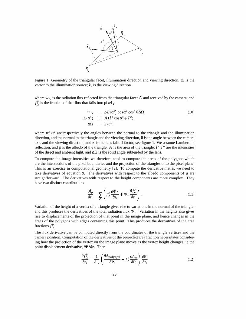
Figure 1: Geometry of the triangular facet, illumination direction and viewing direction.zs is thevector to the illumination source;zv is the viewing direction.

whereΦ4 is the radiation flux reflected from the triangular facet4 and received by the camera, andf p4 is the fraction of that flux that falls into pixelp.

Φ4 = ρE(αs) cosαv cosκ θ∆Ω; (10)

E(αs) = A (I s cosαs+ I a) :

∆Ω = S=d2:

whereαs;αv are respectively the angles between the normal to the triangle and the illuminationdirection, and the normal to the triangle and the viewing direction,θ is the angle between the cameraaxis and the viewing direction, andκ is the lens falloff factor, see figure 1. We assume Lambertianreflection, andρ is the albedo of the triangle.A is the area of the triangle,I s;I a are the intensitiesof the direct and ambient light, and∆Ω is the solid angle subtended by the lens.

To compute the image intensities we therefore need to compute the areas of the polygons whichare the intersections of the pixel boundaries and the projection of the triangles onto the pixel plane.This is an exercise in computational geometry [2]. To compute the derivative matrix we need totake derivatives of equation 9. The derivatives with respect to the albedo components ofu arestraightforward. The derivatives with respect to the height components are more complex. Theyhave two distinct contributions

∂I p

∂zi= ∑

4

f p4

∂Φ4

∂zi+Φ4

∂ f p4

∂zi

!: (11)

Variation of the height of a vertex of a triangle gives rise to variations in the normal of the triangle,and this produces the derivatives of the total radiation fluxΦ4. Variation in the heights also givesrise to displacements of the projection of that point in the image plane, and hence changes in theareas of the polygons with edges containing this point. This produces the derivatives of the areafractions f p

4.

The flux derivative can be computed directly from the coordinates of the triangle vertices and thecamera position. Computation of the derivatives of the projected area fraction necessitates consider-ing how the projection of the vertex on the image plane moves as the vertex height changes, ie thepoint displacement derivative,∂P=∂zi . Then

∂ f p4

∂zi=

1A4

∂Apolygon

∂Pi f p

4

∂A4∂Pi

!∂Pi

∂zi(12)

23

Figure 2: Two images rendered from the synthetic Death Valley surface

50100

150200

250300

350

50

100

150

200

250

300

350

05

101520

Figure 3: Surface reconstructed from the images in figure 2

which shows that to compute the derivative of the area fraction we need to compute the derivative ofthe triangle area,A4, and the polygon areas,Apolygon. These derivatives can be computed by a verygeneral algorithm that considers one edge of the polygon at a time, and accumulates the contributionsto the derivative.

The point displacement derivatives,∂P=∂zi can be derived from the definition of the simple perspec-tive sensor [3], where

Px =[AR(P t)]x[R(P t)]z

(13)

A is the matrix of camera internal parameters,R is the rotation matrix andt the position of thecamera. The point displacement derivatives are given in [4].

Figure 2 shows two of the four images rendered from an artificial surface. The surface was generatedby taking a USGS digital elevation model for Death Valley, and using the intensities from a co-registered Landsat-TM image as surrogates for the albedos. Figure 3 shows the surface reconstructedfrom the four images. Further details can be found in [5].

24

References

[1] J. Foley, A. van Dam, S. Finer, and J. Hughes.Computer Graphics, principles and practice.Addison-Wesley, 2nd ed. edition, 1990.

[2] J. O’Rourke.Computational Geometry in C. Cambridge University Press, 1993.

[3] G. Xu and Z. Zhang Epipolar Geometry in Stereo, Motion and Object Recognition. Kluwer,1996.

[4] R.D. Morris, V.N. Smelyanskiy and P.C. Cheeseman.Matching Images to Models – CameraCalibration for 3-D Surface Reconstruction. Submitted to EMMCVPR 2001, Sophia Antipolis,September 2001.

[5] V.N. Smelyanskiy, P. Cheeseman, D.A. Maluf and R.D. Morris.Bayesian Super-Resolved Sur-face Reconstruction from Images. In Proceedings of Conference on Computer Vision and PatternRecognition, Hilton Head Island, 2000 (CVPR 2000).

25

Geophysical applications of MCMC: Bayesiancalculations and MC-optimization with slowforward algorithms

Klaus Mosegaard (klaus@gfy.ku.dk)

Department of Geophysics, University of Copenhagen, Denmark

Monte Carlo methods are becoming increasingly important for solution of non-linear inverse prob-lems in two different, but related, situations. In the first situation we need a near optimal solution(measured in terms of data fit and adherence to given constraints) to the problem. In the secondsituation, the inverse problem is formulated as a search for solutions fitting the data within a cer-tain tolerance, given by data uncertainties. In a non-probabilistic setting this means that we searchfor solutions with calculated data whose distance from the observed is less than a fixed, positivenumber. In a Bayesian context, the tolerance is “soft”: a large number of samples of statisticallynear-independent models from the a posterior probability distribution are sought. Such solutions areconsistent with the data as well as the available prior information.

Early examples of solution of inverse problems by means of Monte Carlo methods are abundant ingeophysics and other disciplines of applied physics. SinceKeilis-Borok and Yanovskaya[1967] andPress[1968, 1971] made the first attempts at randomly exploring the space of possible Earth modelsconsistent with seismological data, there has been considerable advances in computer technology,and therefore an increasing interest in these methods. Recently, Bayes theorem and the Metropolisalgorithm have been used for calculating approximate a posteriori probabilities for inverse problems(see, e.g.,Pedersen and Knudsen[1990], Koren et al.[1991], Gouveia and Scales[1998], Dahl-Jensen et al.[1999], Khan et al.[2000], Rygaard-Hjalsted et al.[2000], and Khan and Mosegaard[2001]).

Most applications of Monte Carlo Methods for inversion suffer from the major problem that misfitcalculations are so computer intensive, and the model parameter space is so vast, that, in practice,only relatively few models can be sampled. This has led to the development of methods that seekto obtain (in some sense) optimum results within a given (fixed) number of iterations. Some of themost successful of these methods are based on ideas borrowed from statistical mechanics (Nultonand Salamon[1988]).

26

Bayesian inversion of boundary value data

Geoff Nicholls (nicholls@math.auckland.ac.nz)

Department of Mathematics, University of Auckland, New Zealand

Colin Fox (fox@math.auckland.ac.nz)

Department of Mathematics, University of Auckland, New Zealand

Electrical conductivity imaging is one of several non-invasive imaging techniques in which an objectis probed by irradiating it with waves of current, heat or ultrasound, and measurements are made ofthe scattered field. The imaged quantityσ is then related to the wave fieldu by

Electrical ∇ σ∇u = 0

Thermal ∇ σ∇u =∂u∂t

Acoustic ∇ σ∇u =σc2

∂2u∂t2

In each of these canonical expressions the “forward problem” (fromσ to u) requires solution of thecorresponding boundary, or initial-boundary value problem in two or three dimensions. To recoverthe image,σ we must solve the “inverse problem”, which is ill-posed and non-linear.

Exact inverses have been found for some of these problems (see for example [3]). However, anal-ysis shows that the linearised forward problems above have singular values that decrease at leastgeometrically (for example [1]) and hence any inverse must be discontinuous and will give imagesdominated by noise. This inherent ill posed behaviour is actually severe since, in the presence ofnoise, only a limited amount of information aboutσ is transmitted through the forward map. Con-sequently, any image reconstruction algorithm must provide information that is not available in themeasurements. To make best use of the information that is measurable, algorithms must use accuratemodels of both the forward map and noise process. Finally, we would like to quantify uncertaintyin our “solution”. A solution is not a single image, it is a distribution over more or less plausibleimages. We are not aware of any inferential framework which meets all these criteria, unless it be anessentially Bayesian inferential scheme, with a physics-based likelihood.

New sampling methodologies open up the possibility of sampling distributions involving such like-lihoods, and thereby carrying out sample-based Bayesian inference. We focus on the conductivityimaging problem, and a corresponding family of Markov chain Monte carlo algorithms. Such al-gorithms require millions of likelihood ratio evaluations, in each of which a number of Green’sfunctions must be computed. Over the last few years, we have been investigating methods to makethis iterative calculation tractable. We are particularly concerned with the order of one likelihoodratio calculation, as a function of the number of elements in the finite element and boundary elementschemes used to solve for the Green’s function of the forward problem. It seems hard to go past alocal linearisation scheme [2], which is order constant in the number of elements. However, we willdiscuss a wide range of Markov chain Monte carlo schemes, including Langevin and hybrid algo-rithms, and algorithms related to continuous time MCMC, and consider how they may be coupledto numerical methods for solving the forward boundary value problem.

In order to solve an inverse problem, it is not necessary to invert anything, except possibly our wayof thinking.

27

References

[1] C. Fox. Conductance Imaging. PhD thesis, University of Cambridge, 1989.

[2] C. Fox and G. K. Nicholls. Sampling conductivity images via MCMC. In K.V. Mardia, R.G.Ackroyd, and C.A. Gill, editors,The Art and Science of Bayesian Image Analysis, Leeds AnnualStatistics Research Workshop, pages 91–100. University of Leeds, 1997.

[3] J. Sylvester and G. Uhlman. A global uniquness theorem for an inverse boundary value problem.Ann. Math., 125:643–667, 1987.

28

Posterior distributions for numerical weather forecasts

Douglas Nychka (nychka@cgd.ucar.edu)

National Center for Atmospheric Research, Boulder, USA

Thomas Bengtsson and Chris Snyder

National Center for Atmospheric Research, Boulder, USA

Given sparse irregular observation functionals of the atmosphere, the goal is to update the estimateof the current state of the atmosphere and then to use this update to forecast ahead in time. Theupdating step is a huge inverse problem, perhaps the largest solved on a routine basis; the numberof observations is on the order of 105 and the state vector describing the atmosphere is 106. Thistalk reports our research to find computable, Bayesian solutions to this problem. The focus is onan ensemble technique (i.e. Monte Carlo sampling) to estimate reasonable regularizing penaltiesthat adapt to the changing state of the atmosphere and provide credible posterior probabilities. Aninteresting statistical problem is to estimate regularization parameters sequentially because the largesize of this problem does not allow for storage of previous forecasts.

Ensemble forecasting is used in numerical weather prediction to give an improved estimate of theatmospheric state and provide measures of forecast accuracy. Essentially one carries along a set offorecasts where the spread among the group is a measure of forecast uncertainty and the group meanis interpreted as the best single forecast. While the method is effective, there are some fundamentalissues in interpreting the ensemble as a statistically valid representation of uncertainty in the state ofthe atmosphere. In Bayes language, in what sense does the distribution among ensemble membersapproximate a posterior distribution for the state vector? Coupled with this interpretation is thedifficulty in the specification of large, complex covariance matrices used to combine a numericalforecast with observed data. We approach this problem by representing the prior distribution as amixture of Gaussian distributions, then generate an ensemble as a random sample from the posterior.A crucial step in this process to go backwards from an ensemble to a prior distribution for the nextforecast cycle. Here we use a kernel density estimate. The bandwidth in this kernel approximation isan important tunable parameter and we construct a sequential estimate using discrepancies betweenthe forecasts and the observed data.

29

Bayesian inversion in reservoir characterization withcomplex forward models

Henning Omre (omre@math.ntnu.no)

Department of Mathematical Sciences, Norwegian University of Science and Technology, Trond-heim, Norway

Ole Petter Lødøen (olelod@math.ntnu.no)

Department of Mathematical Sciences, Norwegian University of Science and Technology, Trond-heim, Norway

Problem setting

Reliable forecasts of production from petroleum reservoirs are crucial for efficient reservoir man-agement. These forecasts must be based on general reservoir knowledge and reservoir specific ob-servations.

Consider a reservoir with production start at timet0, and let time for evaluation bete, with te t0.The production variables, containing oil production-rate, gas-oil ratio, bottom-hole pressure etc., istermedpt ; t 2 [t0;∞). The production is crucially dependent on the reservoir variables,rx;x 2 D,containing porosity, permeability etc. in the three dimensional reservoir domainD. The reservoirspecific observations contain seismic amplitude data coveringD, ds; observations along the welltrace,dw; and production history observed in time[t0; te), dp.

Focus of the study is on forecasting future production,pt ; t 2 [te;∞), termedpt+ , based on the avail-able information. The time reference,t, is continuously defined, but in practicept will be a finite-dimensional vector on a grid along the time axis.

Stochastic model

The problem is solved in a Bayesian inversion setting, see Omre and Tjelmeland (1997), and themodel is presented in the graph in Figure 1.

A prior model for the reservoir variables,Rx, is represented by the probability density function(pdf), f (rx). These variables are linked to the production variables by a fluid flow simulator,Pt =ω(Rx). Implicitly in this is a recovery strategy for oil, i.e. a well design and injection procedure,defined. The simulator is assumed to be perfect, i.e. it linksPt andRx without error, f (pt jrx). Thereservoir specific observations are linked to(Pt ;Rx) through likelihood modelsf (dsjrx), f (dwjrx)and f (dpjpt). The two former are defined in Eide et al.(1999) and Buland and Omre (2000). Thelatter representspt in the time interval[t0; te), termedpt , with an additive Gaussian observationerror.

The reservoir is usually evaluated at two stages:

Appraisal stage, withte = t0, and the posterior pdf of interest being:

f (pt jds;dw) =

Zf (pt jrx) f (rxjds;dw)drx (14)

30

Production stage, withte t0, and the posterior pdf of interest being:

f (pt+ jds;dw;dp) = f1(dp)

Z Zf (dpjpt) f (pt jrx) f (pt+ jrx) f (rxjds;dw)drxdpt (15)

Sampling procedure

The posterior models are not analytically tractable, primarily due to strong non-linearity in the fluidflow simulatorω(). Moreover, it may take days, or even weeks, to run one forward model inω(). This makes general purpose sampling algorithms like rejection sampling, SIR, Kitanidis-Oliver algorithm and McMC-algorithms unsuitable, see Omre (2000).

In order to improve the sampling, an approximate fluid flow simulator is defined,pt = ω(rx). Thismay be done by solving the differential equations involved on a coarser mesh. The productionvariables are assumed to be linked to the approximate ones through,

f (pt jpt )!Gauss(Apt ;Σ) (16)

with A andΣ being unknown parameters.

The forecast of production can then be written as:

appraisal stage:

f (pt) =Z

f (pt jpt ) f (pt )dpt (17)

production stage:

f (pt+ jdp) = f1(dp)Z Z

f (dpjpt) f (pt jpt ) f (pt+ jp

t ) f (pt )dptdpt (18)

The conditioning on(ds;dw) is implicitly done throughpt and is not shown in the notation.

The following sampling is performed:

r ix; i 2 f1; :::;ng iid f (rxjds;dw) (19)

and

pit = ω(rix); i 2 f1; :::;ng (20)

This can be done with small computational cost even for largen. Based on this, an estimate of thepdf f (pt ) can be made:f (pt ).

Considerf1; :::;mg being a subset off1; :::;ng with m n. Compute:

pjt = ω(r j

x); j 2 f1; :::;mg (21)

Each computation will be very computationally expensive. Based on(pjt ; p j

t ); j 2 f1; :::;mg esti-mates forA andΣ can be made and hence an estimatef (pt jpt ) can be obtained. Note that theselection of the subsetf1; :::;mg amongf1; :::;ngmay be optimized.

The estimated forecasts of production can be based on:

31

appraisal stage:

f (pt) =

Zf (pt jp

t ) f (pt )dpt (22)

production stage:

f (pt+ jdp) = f1(dp)

Z Zf (dpjpt) f (pt jp

t ) f (pt+ jp

t ) f (pt )dptdpt (23)

The former estimate is straight forward to compute. While the latter can be determined by a proce-dure similar to the SIR algorithm. Note that the uncertainty related to using the approximate fluidflow simulator instead of the correct one will be reflected in the production forecast uncertainty.

Example

The example is based on the study in Hegstad and Omre (1999). The setting is as in Figure 1.The correct fluid flow simulator,ω(), is based on a(50 50 15) discretization, and each runrequires 24 hours processing time. The approximate simulator,ω(), is based on a(101015)discretization and can be run in less than five minutes.

*

Reservoir Specific Observations

d pdds w

Reservoir Variables

Production

ApproximateProduction

R

P

Pt

t

x

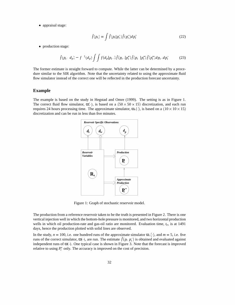
Figure 1: Graph of stochastic reservoir model.

The production from a reference reservoir taken to be the truth is presented in Figure 2. There is onevertical injection well in which the bottom-hole pressure is monitored, and two horizontal productionwells in which oil production-rate and gas-oil ratio are monitored. Evaluation time,te, is at 1491days, hence the production plotted with solid lines are observed.

In the study,n= 100, i.e. one hundred runs of the approximate simulatorω(), andm= 5, i.e. fiveruns of the correct simulator,ω(), are run. The estimatef (pt jpt ) is obtained and evaluated againstindependent runs ofω(). One typical case is shown in Figure 3. Note that the forecast is improvedrelative to usingPt only. The accuracy is improved on the cost of precision.

32

0 1000 2000 30000

5000

10000

15000

OPR 1

0 1000 2000 30000

5000

10000

15000

OPR 2

0 1000 2000 30003500

4000

4500

5000

5500

6000

6500

7000BHP

0 1000 2000 30000

2

4

6

8

10GOR 1

0 1000 2000 30000

2

4

6

8

10GOR 2

Figure 2: Production variables from reference reservoir

0 1000 2000 30000

5000

10000

15000

OPR 1

0 1000 2000 30000

5000

10000

15000

OPR 2

0 1000 2000 30000

2

4

6

8

10GOR 1

0 1000 2000 30000

2

4

6

8

10GOR 2

0 1000 2000 30003500

4000

4500

5000

5500

6000

6500

7000BHP

Figure 3: Forecast of one arbitrary realization,rx.pt = ω(rx):— ; pt = ω(rx) :- - -; f (pt jpt ) : exp--- , 0.80 interval ---

33

In Figure 4, estimated forecast of production,f (pt+ jdp), is presented. Note that if onlym= 5 runsof the correct simulator are possible, none of the general purpose sampling algorithms can be used.

0 1000 2000 30000

5000

10000

15000

OPR 1

0 1000 2000 30000

5000

10000

15000

OPR 2

0 1000 2000 30003500

4000

4500

5000

5500

6000

6500

7000BHP

0 1000 2000 30000

2

4

6

8

10GOR 1

0 1000 2000 30000

2

4

6

8

10GOR 2

Figure 4: Forecast at production stage:f (pt+ jdp) : exp--- , 0.80 interval --- .Reference production: observed—, future —

References

See www.math.ntnu.no/omre/recentwork.html and references therein.

34

Quantitative analysis of data from PET imaging studies

Finbarr O’Sullivan (finbarr@stat.ucc.ie)

Department of Statistics, University College Cork, Ireland

Positron emission tomography (PET) is a radiological imaging technique that has the ability to mea-sure metabolic characteristics of tissue in-vivo. Statisticians are familiar with the reconstructionproblem of PET which involves the inversion of the Radon transform based on scaled Poisson datato produce estimates of the distribution of activity of an injected radio-tracer.

Data sets arising from PET studies involve dynamic volumetric scans representing the temporallyintegrated time-course of the distribution of a radiotracer and its metabolites in a tissue region. Doseconstraints on the injected radio-tracer place critical limitations on the spatial and temporal accuracyof the data. In modern PET machines the nominal spatial resolution of scans is between 2 and 5mm.Temporal sampling varies with the radiotracer used - there can be as many as 1 scan per second toperhaps as few as 2 scans per hour. A typical data set would be on the order of 140Mb in size.

A range of statistical methodologies, including semi-blind deconvolution, image segmentation, mix-ture modeling, non-linear functional estimation arise in the context of the analysis of modern PETstudies. This talk presents an overview of research conducted on the development of these techniquesin the context of two primary applications: (i) Construction of functional images for brain and car-diac studies, and (ii), Assessment of tissue heterogeneity for human sarcoma. Data from on-goingstudies conducted at the University of Washington, PET imaging facility are used for illustration.

35

Spectral methods for noisy integral equations

Frits H. Ruymgaart (ruymg@math.ttu.edu)

Department of Mathematics and Statistics, Texas Tech University, Lubbock, USA

Inverse estimation concerns the recovery of an unknown input signal from blurred observations ona known transformation of that signal. The estimators of such indirectly observed curves to beconsidered here are derived from a regularized inverse of the transformation involved, exploitingHalmos’s (1963) version of the spectral theorem. The usual criterion for asymptotic optimality ofsuch curve estimators is based on the mean integrated squared error. It will be seen that the proposedestimators are rate optimal in general. One may also consider optimality related to weak convergencein the sense of Ha’jek’s (1970) ”convolution” theorem and its generalizations as developed in van derVaart (1988). The curve estimators induce natural estimators for certain linear functionals that turnout to be optimal in the case of indirect density estimation. However,the estimators are not in generaloptimal in the indirect regression model, except when the errors are normal. This suboptimality isdue to the error density that plays the role of a nuisance parameter.

36

Inverse problems in helioseismology

Philip B. Stark (stark@stat.berkeley.edu)

Department of Statistics, University of California, Berkeley, USA

The Sun vibrates constantly in a superposition of acoustic normal modes excited by turbulence inthe Suu’s convective zone. The modes have a velocity amplitude of about 1cm/s in the photosphere.They have characteristic periods on the order of 5 minutes, lifetimes ranging from hours to months,and are excited many times per lifetime. The Sun is thought to support about 107 modes; about3105 have been observed.

Each mode has two quantum numbers, l and m, that characterize its angular dependence, and a thirdquantum number, n, that characterizes its radial dependence. If the Sun were spherically symmetricaland did not rotate, the

freguencies of the 2l +1 modes with the same values ofl andn would have the same temporal fre-quency; that frequency is related to soundspeed as a function of radius by an Abel transform. TheSun rotates, but not rigidly. Differential rotation splits the 2l +1 degenerate frequencies symmetri-cally. Asphericity of material properties splits the 2l +1 degenerate frequencies asymmetrically; thissplitting is a weighted average of the rotation rate as a function of radius and latitude. The frequen-cies of the modes thus contain information about the composition, state, and kinematics of the solarinterior. Extracting estimates of solar structure and kinematics from the normal mode frequenciesare the fundamental inverse problems of normal mode helioseismology.

However, estimating the frequencies of the modes is itself an inverse problem, whose ill-posedness isexacerbated by gaps in the spatio-temporal data. Two current experiments take different approachesto reducing diurnal gaps: the SOHO project observes the Sun from orbit around the L1 Lagrangepoint, where the Sun never sets; the GONG network of solar telescopes spans the globe at midlatitudes, so the Sun never sets on the network. Neither experiment can observe as much as half thesurface of the Sun at one time, and both suffer from occasional data loss, so there are gaps in thedata.

I will present an approach to estimating solar oscillation frequencies that mitigates the problemscaused by gaps by tailoring apodizing windows to the gap structure in an optimal way. The work,joint with I.K. Fodor, extends work by Thompson, Riedel, Sidorenko, Bronez and others on optimaltapering. Computing optimal tapers is very demanding computationally, but there is an inexpensiveapproach that is nearly optimal in practice for typical helioseismic data. The frequencies of morenormal modes can be identified from these spectrum estimates than from estimates used previouslyby the GONG project. Calculating confidence intervals for the multitaper spectrum estimates provesto be challenging: existing methods–including parametric approximations and a variety of resam-pling plans in the time and frequency domains–fail, partly because of the dependence structure of thedata. A novel resampling approach yields (apparently) conservative confidence intervals. Researchis underway to extend the approach to estimate the spatial spectra from spherical data.

37

Nonparametric study of differential equationsand inverse problems

Anne Vanhems (anne.vanhems@univ-tlse1.fr)

Gremaq and Crest, University Toulouse, France

The aim of our work is to provide a general framework for studying nonparametrically differentialequations. We intend to replace our study in the context of inverse problems as treated by Tikhonovand Arsenin (1977) and to link it with economic issues.

Therefore, let us consider independent identically distributed observations which admit an unknowncumulative density functionF . Structural econometrics considers implicit transformation ofF . Ofcourse, the theory developped depends on the nature and properties of the transformation considered.For example, there exists a wide literature about integral transformations, like additive models orinstrumental variables theory. We are interested in studying differential transformations ofF, andby extension of the conditional expectation. In a general way, we want to characterize the solutionsof ordinary differential equations of that kind:

y0 = m(x;y;F)y(x0) = y0

wherey2 IR and m : IR IRz(IR)! IR is, for the moment, continuous. We want first to studythe existence and unicity of a solution, that is formally to inverse a differential operator. Second, ourobjective is to consider the solution, if it exists, of the following system:(

y0 = m

x;y; bFy(x0) = y0

At last, we will study the asymptotic properties of these two solutions.

Such a purpose can be justified first by the numerous applications in economics. For example, in amicroeconomic context, Hausman and Newey (1995) estimate nonparametrically the exact consumersurplus by solving a differential equation. In physics, Florens and Vanhems (2000) find the estimatorof the ionosphere thickness by solving a differential equation given by physics theory. In finance,Ait-Sahalia (1996) studies the prices of derivative securities by solving a Cauchy problem.

Second, the properties of solutions of such systems are attractive. We all know that integratinga nonparametric estimator will improve its properties. More generally, we want to examine theproperties of integral operators on a nonparametric estimator, and to show that it will improve it.

References

[1] Ait-Sahalia, Y. (1993). The delta and bootstrap methods for non parametric kernel functionals.Preprint

[2] Ait-Sahalia, Y. (1996). Nonparametric pricing of interest rate derivative securities.Economet-rica, Vol.64, 527-560

[3] Bosq, D. (1996). Non parametric statistics for stochastic processus.Springer-Verlag

38

[4] Choquet, G. (1964). Cours d’analyse tome II Topologie.Masson et Cie

[5] Florens, J.P. and Vanhems, A. (2000). Nonparametric estimation of ionosphere thickness.Preprint

[6] Hausman, J. and Newey, W. K. (1995). Nonparametric estimation of exact consumers surplusand deadweight loss.Econometrica, Vol. 63, 1445-1476

[7] Kunze, H. E. and Vrscay, E. R. (1999). Solving inverse problems for ordinary differential equa-tions using the Picard contraction mapping.Inverse Problems, Vol.15, 745-770

[8] Sibony, M. and Mardon, J.-Cl. (1984). Approximations et equations differentielles.Hermann

[9] Tikhonov, A. N. and Arsenin, V. Y. (1977). Solutions of ill-posed problems.V.H. Winston &Sons

39

Combining observations with models: Penalizedlikelihood and related methods in numericalweather prediction

Grace Wahba (wahba@cs.wisc.edu)

Department of Statistics, University of Wisconsin-Madison, Madison, USA

We will look at variational data assimilation as practiced by atmospheric scientists, with the eyes of astatistician. Recent operational numerical weather prediction models operate on what might be con-sidered a very grand penalized likelihood point of view: A variational problem is set up and solvedto obtain the evolving state of the atmosphere, given heterogenous observations in time and space,a numerical model embodying the nonlinear equations of motion of the atmosphere, and variousphysical constraints and prior physical and historical information. The idea is to obtain a sequenceof state vectors which is ‘close’ to the observations, close to a trajectory satisfying the equations ofmotion, and simultaneously respects the other information available. The state vector may be as bigas 107, and the observation vector 105 or 106, leading to some interesting implementation questions.Interesting non-standard statistical issues abound.

This talk is based partly on

J. Gong, G. Wahba, D. Johnson and J. Tribbia, ‘Adaptive Tuning of Numerical Weather Predic-tion Models: Simultaneous Estimation of Weighting, Smoothing and Physical Parameters, MonthlyWeather Review 125, 210-231 (1998)

A related paper is G. Wahba, ”Adaptive Tuning, four Dimensional Variational Data Assimilation, andRepresenters in RKHS, in ‘Diagnosis of Data Assimilations Systems’, Proceedings of a Workshopheld at the European Centre for Medium-Range Weather Forecasts, Reading, England, March 1999,45-52. Both are available via Grace Wahba’s home page.

40

5 List of speakers and participants

Speakers

Robert S. AnderssenCSIRO Mathematical and Information SciencesGPO Box 664Canberra, ACT 2601AustraliaE-mail: Bob.Anderssen@cmis.csiro.au

Jose M. AnguloDepartment of Statistics and Operations ResearchFaculty of SciencesUniversity of GranadaCampus Fuente Nueva s/nSpainE-mail: jmangulo@ugr.es

Viktor BenesDepartment of Probability and StatisticsCharles UniversityFaculty of Mathematics and PhysicsSokolovska 8318675 Praha 8The Czech RepublikE-mail: benesv@karlin.mff.cuni.cz

Per Christian HansenInformatics and Mathematical ModellingTechnical University of DenmarkRichard Petersens PladsBuilding 3212800 Kongens LyngbyDenmarkE-mail: pch@imm.dtu.dk

Marcela HlawiczkovaDepartment of Probability and Statistics Charles UniversityFaculty of Mathematics aand PhysicsSokolovska 8318675 Praha 8The Czech RepublikE-mail: mhlawiczkova@yahoo.com

Markus KiderlenMathemat. Inst. IIUniversity of Karlsruhe76128 KarlsruheGermanyE-mail: kiderlen@imf.au.dk

Odd KolbjørnsenDepartment of Mathematical SciencesNorwegian University of Science and Technology7491 TrondheimNorwayE-mail: ok@math.ntnu.no

Robin MorrisUSRA-RIACSNASA Ames Research Center, Mail Stop 269-2Moffett Field, CA 94035-1000USAE-mail: rdm@ptolemy.arc.nasa.gov

Klaus MosegaardDepartment of GeophysicsUniversity of CopenhagenJuliane Maries Vej 302100 Cophenhagen ØDenmarkE-mail: klaus@gfy.ku.dk

Geoff NichollsDepartment of MathematicsUniversity of AucklandPrivate Bag 92019AucklandNew Zealandnicholls@math.auckland.ac.nz

Doug W. NychkaGeophysical Statistics ProjectNational Center for Atmosphserical ResearchClimate and Global Dynamics DivisionBoulder, CO 80302USAE-mail: nychka@cgd.ucar.edu

Henning OmreDepartment of Mathematical SciencesNorwegian University of Science and Technology7491 TrondheimNorwayE-mail: omre@math.ntnu.no

Finbarr O’ SullivanDepartment of StatisticsUniversity College CorkCorkIrelandE-mail: finbarr@stat.ucc.ie

Maria D. Ruiz-MedinaDepartment of Statistics and Operations ResearchFaculty of SciencesUniversity of GranadaCampus Fuente Nueva s/nSpainE-mail: mruiz@ugr.es

41

Frits H. RuymgaartDepartment of Mathematics and StatisticsTexas Tech UniversityBox 41042Lubbock, TX 79409-1042USAruymg@math.ttu.edu

Philip B. StarkDepartment of StatisticsUniversity of CaliforniaBerkeley, CA 94720-3860USAE-mail:stark@stat.Berkeley.EDU

Anne VanhemsGremaq - Universit des Sciences SocialesManufacture des Tabacs21, alles de Brienne31000 ToulouseFranceE-mail: anne.vanhems@univ.tlse1.fr

Grace WahbaDepartment of StatisticsUniversity of Wisconsin-Madison1210 West Dayton StreetMadison, WI 53706-1685USAwahba@stat.wisc.edu

Participants

Kim Emil AndersenDepartment of Mathematical SciencesAalborg UniversityFredrik Bajers Vej 7G9220 Aalborg ØDenmarkE-mail: emil@math.auc.dk

Marie Lund AndersenInformatics and Mathematical ModellingTechnical University of DenmarkRichard Petersens PladsBuilding 3052800 Kongens LyngbyDenmarkE-mail: marie915@forum.dk

Ann-Charlotte BerglundInformatics and Mathematical ModellingTechnical University of DenmarkRichard Petersens PladsBuilding 3212800 Kongens LyngbyDenmarkE-mail: acb@imm.dtu.dk

Svend BerntsenDepartment of Mathematical SciencesAalborg UniversityFredrik Bajers Vej 7G9220 Aalborg ØDenmarkE-mail: sb@math.auc.dk

Kasper BerthelsenDepartment of Mathematical SciencesAalborg UniversityFredrik Bajers Vej 7G9220 Aalborg ØDenmarkE-mail: kkb@math.auc.dk

Ole F. ChristensenDepartment of Mathematical SciencesAalborg UniversityFredrik Bajers Vej 7G9220 Aalborg ØDenmarkE-mail: olefc@math.auc.dk

Horia CorneanDepartment of Mathematical SciencesAalborg UniversityFredrik Bajers Vej 7G9220 Aalborg ØDenmarkE-mail: cornean@math.auc.dk

Martin B. HansenDepartment of Mathematical SciencesAalborg UniversityFredrik Bajers Vej 7G9220 Aalborg ØDenmarkE-mail: mbh@math.auc.dk

Sture HolmMatematisk StatistikChalmersSE-41296 G¨oteborgSwedenE-mail: holm@math.chalmers.se

Michael JacobsenInformatics and Mathematical ModellingTechnical University of DenmarkRichard Petersens PladsBuilding 3052800 Kongens LyngbyDenmarkE-mail: mj@imm.dtu.dk

42

Jens Ledet JensenDepartment of Mathematical SciencesTheoretical StatisticsUniversity of Aarhus8000 Aarhus CDenmarkE-mail: jlj@imf.au.dk

Jon JohnsenDepartment of Mathematical SciencesAalborg UniversityFredrik Bajers Vej 7G9220 Aalborg ØDenmarkE-mail: jjohnsen@math.auc.dk

Rikke Høj KjeldsenInformatics and Mathematical ModellingTechnical University of DenmarkRichard Petersens PladsBuilding 3052800 Kongens LyngbyDenmarkE-mail: rikke@ostenfeld.dk

Kim KnudsenDepartment of Mathematical SciencesAalborg UniversityFredrik Bajers Vej 7G9220 Aalborg ØDenmarkE-mail: kim@math.auc.dk

Steffen L. LauritzenDepartment of Mathematical SciencesAalborg UniversityFredrik Bajers Vej 7G9220 Aalborg ØDenmarkE-mail: steffen@math.auc.dk

Roderik V.N. MelnikUniversity of Southern DenmarkMads Clausen InstituteGrundtvigs Alle 1506400 SønderborgDenmarkE-mail: rmelnik@mci.sdu.dk

Jesper MøllerDepartment of Mathematical SciencesAalborg UniversityFredrik Bajers Vej 7G9220 Aalborg ØDenmarkE-mail: jm@math.auc.dk

Steen MøllerDepartment of Mathematical SciencesAalborg UniversityFredrik Bajers Vej 7G9220 Aalborg ØDenmarkE-mail: moeller@math.auc.dk

Anders NielsenDepartment of Mathematics and PhysicsThe Royal Veterinary and Agricultural UniversityThorvaldsensvej 401871 Frederiksberg CDenmarkE-mail: an@dfu.min.dk

Jonny OlssonStatistical NormBomvagen 20226-51 LundSwedenE-mail:jonny.olsson@mailbox.swipnet.se

Frede TøgersenBiometry Research UnitDepartment of Agricultural SystemsResearch Centre FoulumP.O. Box 508830 TjeleDenmarkE-mail: FredeA.Togersen@agrsci.dk

Samuli SiltanenInstrumentarium Corp. Imaging DivisionP.O. Box 2004301 TuusulaFinlandE-mail:samuli.siltanen@fi.instrumentarium.com

Christian Bressen PipperDepartment of Mathematics and PhysicsThe Royal Veterinary and Agricultural UniversityThorvaldsensvej 401871 Frederiksberg CDenmarkE-mail: bressen@dina.kvl.dk

Jan Marthedal RasmussenInformatics and Mathematical ModellingTechnical University of DenmarkRichard Petersens PladsBuilding 3052800 Kongens LyngbyDenmarkE-mail: jmr@imm.dtu.dk

Christian RitzDepartment of Mathematics and PhysicsThe Royal Veterinary and Agricultural UniversityThorvaldsensvej 401871 Frederiksberg CDenmarkE-mail: ritz@dina.kvl.dk

43