inverse modelling of two-phase flow - el rincón de jaime gómez
TRANSCRIPT

UNIVERSIDAD POLITECNICA DE VALENCIA
Departamento de Ingenierıa Hidraulica y Medio Ambiente
INVERSE MODELLING
OF TWO-PHASE FLOW:
CALIBRATION OF RELATIVE
PERMEABILITY CURVES
TESIS DOCTORAL
By
Carolina Guardiola-Albert
Adviser:
Jaime Gomez-Hernandez


Abstract
Stochastic mathematical modeling of multi-phase flow in heterogeneous porous media is
of great interest in petroleum engineering and subsurface hydrology. Reservoir simula-
tion models are essential for the management of petroleum production or remediation
water resources. The stochastic framework gives the possibility to characterize the
natural spatial variability of the flow parameters. Within this stochastic framework,
multiphase flow simulations are used in order to evaluate different recovery or clean
up processes, to make decisions regarding the placement of the wells, and to specify
various operating procedures associated with injection and production wells.
It is common knowledge that inverse modeling theory provides a methodology to
integrate both static and dynamic data in reservoir characterization. The inversion
method can make the model geologically consistent at the same time that it reproduces
parameter measurements and dynamic responses of the reservoir. Production data
integration in reservoir modeling is performed through an inverse technique because
dynamic data are non linearly related with reservoir heterogeneous properties through
multiphase flow equations. In fact, the inverse modeling tool is a key factor in drawing
up the field development plan, and for managing the available reserves over time. The
advances in computational algorithms and hardware are continuously improving every
day. New inverse numerical techniques take advantage of these progresses. However,
still remains a practical tool for reservoir characterization which takes into account all
the complex processes and parameters that are important for multiphase flow.
Absolute permeability is one of the parameters that are typically estimated with
inverse flow simulators. The inversion techniques that estimate the spatial distribution
of absolute permeability are commonly apply to multi and single phase flow problems.
During last decades this issue has been submitted to intensive research. However,
when studying multiphase flow there is another important property that complements
absolute permeability. This parameter is relative permeability, which controls the
rate of displacement of the different phases present in the reservoir. Altough relative
permeabilities are so important to characterize the movement of two immiscible fluids,
like oil and water or non aqueous contaminants and water, there are not studies nor
i

ii ABSTRACT
techniques to estimate the spatial distribution of relative permeabilities as it is done
with absolute permeability. Normally these functions are assumed to be equal to
measured values from laboratory experiments performed on core samples. Or, if there
are not core samples available, they are taken from studies with similar geology and
flow configuration.
In any case, if the output value from the core experiment is assigned to represent
the relative permeability value of the whole reservoir, or if the relative permeability
is taken from another reservoir study, the model of the multiphase flow simulator is
subjected to an important source of error. This dissertation proposses to characterize
relative permeabilities assuming that they have a spatial distribution, and estimate
this spatial variability as it is usually done with absolute permeability distributions.
The objective of the research work presented here is to develop a new inverse technique
to estimate both absolute and relative permeabilities spatial distributions from static
parameter measurements and production data, such as pressures and saturations. This
technique has to deal with the non linearities present in the multiphase flow equations.
As relative permeabilities are dependent on one of the state variables (saturations) the
optimization problem is highly non linear, increasing the difficulty of the problem that
has to be solved.
The governing equations for immiscible two-phase flow are formulated in terms of
water saturation and fluid pressure. The proposed formulation simplifies the equation
by disregarding gravity and capillary pressure terms, and using finite differences nu-
merical approach. Calibration of the flow model to non linear data is formulated as
an optimization problem, which tries to minimize some objective function. This objec-
tive function measures the differences between the historical production data (water
breakthrough and pressure changes) and the corresponding simulated values. The
inverse method presented here follows the technique developed in the Sequential Self-
Calibrated method. A computer code, written in C, couples the forward two-phase
flow simulator TOUGH with the iterative inverse method. The optimization algorithm
is based on gradient methods, and the concept of master points is borrowed from
the Sequential Self-Calibrated method to reduce the number of parameters subjected
to calibration. After calibration, the result is one equally likely reservoir realization
honoring historical pressure and saturation data.
Calibration parameters were chosen from the relative permeability expressions in
function of saturation. These parameters are: the two end-points of oil and water rela-
tive permeability functions and the two residual saturations. These four values control
the shape of the relative permeability curves. The method is tested with different synt-
hetic examples in one and two dimensions. All simulations shown in this dissertation
iii
assume that porosity is known. The goal of these examples is to test the applicability
of the method and to study the influence of relative permeability parameters in the dy-
namic behavior of the reservoir. In the implementation different injection/production
configurations have been assumed and different kind of heterogeneities for the relative
permeability function have been proposed.
Results given by several examples of inversion simulations have shown that the
method works. Once the calibration is performed, the result is just one of the possible
representations of the medium. Using multiple equiprobable realizations it is possible
to develop a study of uncertainty of the reservoir model, and then to translate it into
uncertainty of reservoir performance predictions for reservoir management. This way
to carry out an uncertainty analysis is normally known as Monte Carlo simulation.
The objective is to analyze the influence of relative permeability parameters on the
model, as well as on the predictions of the reservoir performance. It has been found
out that uncertainties related with oil and water end-points of the relative permeability
curves are higher than the uncertainties related with residual saturations. In general, it
looks like uncertainties related with the four relative permeability parameters in study
are important. Breakthrough saturation predictions appear to have small uncertainty
when they are forecasted with the inversion technique developed, and to be better
predicted in the first states of the exploitation. The most important conclusion of the
dissertation is the high influence of relative permeability heterogeneities in the values
of the saturation shock front. Hence, the importance of research studies about how
to estimate the spatial distribution of relative permeability parameters and absolute
permeability, in order to improve predictions of the water displacement in two-phase
immiscible flow problems.

iv ABSTRACT

Resumen
Los modelos matematicos estocasticos para la simulacion de flujo multifase en medios
porosos heterogeneos tienen un gran interes en ingenierıa del petroleo e hidrologıa
subterranea. Los modelos de simulacion de yacimientos son esenciales en la gestion
de produccion petrolıfera o en la recuperacion de acuıferos contaminados. El entorno
estocastico da la posibilidad de caracterizar la variabilidad espacial intrınseca de los
parametros de flujo. Dentro de este marco estocastico, la simulacion de flujo multifase
se usa para poder evaluar los diferentes procesos de recuperacion o limpieza, y ası
tomar decisiones con respecto al emplazamiento de los pozos o a los procedimientos
asociados a los bombeos o las inyecciones.
La teorıa de modelizacion inversa da la posibilidad de integrar variables estaticas
y dinamicas en la caracterizacion del yacimiento. El metodo inverso puede hacer que
el modelo sea geologicamente consistente al mismo tiempo que reproduce las medidas
de los parametros y las repuestas dinamicas del medio. La integracion de los datos
de produccion en la modelizacion del yacimiento se realiza a traves de las tecnicas de
modelizacion inversa porque los datos dinamicos estan relacionados de forma no lineal
con las propiedades heterogeneas del yacimiento por las ecuaciones de flujo multifase.
De hecho, la modelizacion inversa es un factor clave a la hora de planificar el plan
de desarrollo de un campo petrolıfero, o para la gestion de las posibles reservas a
explotar. Los avances en algorimos de computacion y hardware mejoran dıa a dıa.
Los metodos mas modernos hacen uso de estos avances para mejorar la rapidez en la
simulacion de flujo. Sin embargo, todavıa no existe una herramienta que sea practica
y que ademas tenga en cuenta todos los procesos y parametros que son importantes en
el flujo multifase.
La permeabilidad absoluta es uno de los parametros que que son tıpicamente esti-
mados por medio de simulaciones inversa de flujo. Las tecnicas de simulacion inversas
que estiman la distribucion espacial de la permeabilidad absoluta se utilizan normal-
mente tanto en problemas de flujo de multifase como para flujo de una sola fase. En
las ultimas decadas este tema ha sido sujeto de intensas investigaciones. En cambio,
cuando se estudia flujo multifase hay que tener en cuenta otra propiedad que com-
v

vi RESUMEN
plemente la permeabilidad absoluta, y que es muy importante. Este parametro es la
permeabilidad relativa, que controla la tasa de desplazamiento de las diferentes fases
presentes en el yacimiento. A pesar de que la permeabilidad relativa es muy importante
para caracterizar el movimiento de dos fluidos inmiscibles, como por ejemplo el agua
y el petroleo o el agua y un contaminante no acuoso, no existen estudios o tecnicas
que estimen la distribucion espacial de las permeabilidades relativas como se hace ha-
bitualmente con la permeabilidad absoluta. Normalmente, estas funciones se suponen
conocidas, cuyo valor se toma de medidas en laboratorio tomadas en testigos. En el
caso de que no hayan testigos, las permeabilidad relativas se asignan por similitud con
otros yacimientos de geologıa y condiciones de flujo similares.
En cualquier caso, si se asume que el valor obtenido en el laboratorio representa el
valor de la permeabilidad relativa en todo el yacimiento, o incluso si se toma de otro
yacimiento similar al de estudio, el modelo del flujo multifase experimentara impor-
tantes errores. Esta tesis doctoral propone caracterizar las permeabilidades relativas
asumiendo que tienen variabilidad espacial, y estimar esta variabilidad espacial como
se hace normalmente con las distribuciones de permeabilidad absoluta. El objetivo
del trabajo de investigacion que se presenta a continuacion es desarrollar una nueva
tecnica de simulacion inversa que estime la distribucion espacial de las permeabilida-
des absoluta y relativa a partir de las medidas de parametros estaticos y los datos
de produccion, como las presiones y las saturaciones. Esta tecnica tiene que tener en
cuenta las no linearidades que existen en las ecuaiones de flujo multifase. Al ser la per-
meabilidades relativas dependientes de una de las variables de estado (la saturacion)
el problema de optimizacion el altamente no lineal, incrementando las dificultades del
problema a resolver.
Las ecuaiones que gobiernan el flujo inmiscible bifase estan formuladas en terminos
de las saturaciones y las presiones. Ademas, las ecuaciones se simplifican desestimando
las fuerzas gravitatorias y capilares, y usando aproximacion numerica por diferencias
finitas. La calibracion del modelo de flujo a los datos no lineales se expresa como un
problema de optimizacion, que minimiza una funcion objetivo. Esta funcion objetivo
mide las diferencias entre los datos historicos de produccion y los valores simulados
correspondientes. El metodo inverso que se presenta en esta tesis sigue la tecnica
desarrollada por el metodo autocalibrante. Se ha escrito un codigo, en lenguaje C,
que acopla el modelo de flujo directo TOUGH con el metodo inverso iterativo. El
algoritmo de optimizacion se basa en el metodo de los gradientes, y el concepto de
puntos maestros se toma prestado del metodo autocalibrante para reducir el numero
de parametros que se van a calibrar. Despues de realizar una calibracion se obtiene
una realizacion, que una mas del conjunto de realizaciones posibles que reproducen los

vii
datos de saturacion y presion.
Los parametros elegidos para la calibracion se toman de las expresiones de las per-
meabilidades relativas en funcion de la saturacion. Estos parametros son: los dos
puntos finales de las curvas de permeabilidad relativa del agua y del petroleo y las
saturaciones residuales. Estos cuatro parametros controlan el tamano y la forma de
las curvas de permeabilidad relativa. Se ha probado el metodo con varios ejemplos
sinteticos en una y dos dimensiones. En todas las simulaciones mostradas en esta tesis
la porosidad es conocida. El objetivo de estos ejemplos es mostrar que el metodo es
aplicable y estudiar la influencia de la distribucion espacial de los parametros de la per-
meabilidad relativa. Se han probado distintas configuraciones de inyeccion/produccion
y diferentes tipos de heterogeneidad para las curvas de permeabilidad relativa.
Los resultados dados en distintos ejemplos de simulaciones inversas han demostrado
que el metodo funciona. Una vez que la calibracion se ha realizado, el resultado es una
posible representacion del yacimiento. Usando multiples realizaciones equiprobables es
posible desarrollar un estudio de incertidumbre del modelo del yacimiento, para trasla-
darlo a incertidumbres en las predicciones de gestion del mismo. Esta forma de realizar
un estudio de incertidumbre es lo que comunmente se conoce como simulacion de Monte
Carlo. El objetivo es analizar la influencia de los parametros de permeabilidad relativa
en el modelo, ası como en las predicciones del funcionamiento del yacimiento. Los re-
sultados encontrados en este trabajo de investigacion muestran que las incertidumbres
relacionadas con los puntos finales de las curvas de permeabilidad relativa son mayores
que las incertidumbres relacionadas con las saturaciones residuales. En general parece
que las incertidumbres para los cuatro parametros que se calibran son bastante impor-
tantes. Las predicciones de los datos de saturacion tienen menor incertidumbre cuando
se predicen con la tecnica aquı desarrollada, y se obtienen mejores resultados para los
primeros tiempos de explotacion del yacimiento. La conclusion mas importante que
aporta este trabajo es la gran influencia que tienen las heterogeneidades de las curvas
de permeabilidad relativa en los valores de saturacion. Es por ello que es muy impor-
tante que los estudios sobre como estimar la distribucion espacial de la permeabilidad
absoluta y relativa continuen y sobretodo que se consigan algoritmos mas rapidos para
hacer estudios de mayores dimensiones mas reales.

viii RESUMEN

Resum
ix

x RESUM

Agradecimientos
Esta tesis ha sido posible gracias a la ayuda y apoyo de muchas personas que me
han acompanado durante estos anos. En primer lugar quiero agradecer a mi director
de tesis, Jaime Gomez-Hernandez, por darme la oportunidad de hacer este trabajo
de investigacion. Sin sus ideas, propuestas y supervision este trabajo simplemente no
existirıa. Quiero agradecerle tambien los consejos que me ha dado, los ’entrenamientos’
en las exposiciones, y todas las oportunidades que me ha ofrecido.
La fundacion Repsol-YPF y la Empresa Nacional de Residuos Radioactivos S.A.
(ENRESA) a traves de la Universidad Politecnica de Valencia han financiado estos
anos de investigacion.
Mis companeros de departamento me han ayudado en los problemas del dıa a dıa
y ademas han hecho que mi experiencia en Valencia sea inolvidable. En especial me
gustarıa agradecer a Eduardo Cassiraga por sus animos para que realizase la tesis en la
UPV, su ayuda y su amistad durante estos anos. A Rafael Aliaga, companero de luchas
con linux y demas problemas informaticos, siempre dispuesto a ayudarme y animarme.
A Harrie Hendricks-F., por su legado de INVERTO. A Andres Sahuquillo, Edu, Rafa,
Harrie, Claudia, Lourdes, Carmen, Carlos, Hector, y JianLin por todas las horas de
convivencia y por hacer mas agradables los momentos de trabajo. Por supuesto me
siento agradecida a todos los ’materos’, por la companıa en los descansos y por las
risas, las comidas en derecho y las tertulias en Dos Hermanos. A Andres, Julian y
Andrea por su amistad y su apoyo. A Guey, por la gran amiga que he ganado.
Fuera del departamento no me puedo olvidar de Jose, Manuela, Victor, Ivan y los
demas del grupo, por cuidarme tanto y hacer que no me sintiera una extrana en esta
ciudad, por los momentos en el Roca. A todos mis amigos de Madrid, por el apoyo en
la distancia. Habrıa mucha mas gente que mencionar, que estan o han estado cerca de
mı. Las limitaciones de espacio no me permiten escribir sus nombres, aunque ello no
significa que hayan sido menos importantes en estos anos. Le agradezco enormemente
a mis padres su apoyo y su confianza en mı. A mi padre su asesoramiento constante
en programacion en C y FORTRAN, y en los problemas con linux.
Finalmente quiero dedicar esta tesis a Carlos, por su amor y su espera.
xi

xii AGRADECIMIENTOS

Contents
Abstract i
Resumen v
Resum ix
Agradecimientos xi
Nomenclature xxiii
1 Introduction 1
1.1 Motivation and scope . . . . . . . . . . . . . . . . . . . . . . . . . . . . 1
1.2 Stochastic inverse modeling . . . . . . . . . . . . . . . . . . . . . . . . 3
1.3 Why calibration of krel? . . . . . . . . . . . . . . . . . . . . . . . . . . 5
1.4 Objectives and dissertation outline . . . . . . . . . . . . . . . . . . . . 6
2 Literature Review 9
2.1 The beginnings . . . . . . . . . . . . . . . . . . . . . . . . . . . . . . . 9
2.2 Current numerical approaches . . . . . . . . . . . . . . . . . . . . . . . 10
2.2.1 The choice of primary variables . . . . . . . . . . . . . . . . . . 12
2.2.2 Numerical approximation . . . . . . . . . . . . . . . . . . . . . 15
2.3 Inverse stochastic simulation . . . . . . . . . . . . . . . . . . . . . . . . 17
2.3.1 Stochastic framework . . . . . . . . . . . . . . . . . . . . . . . . 17
2.3.2 Inverse modeling problem . . . . . . . . . . . . . . . . . . . . . 18
2.3.3 Ill-posedness . . . . . . . . . . . . . . . . . . . . . . . . . . . . . 19
2.3.4 Optimization algorithms . . . . . . . . . . . . . . . . . . . . . . 20
2.4 Inverse modeling methods . . . . . . . . . . . . . . . . . . . . . . . . . 22
2.4.1 Cokriging method . . . . . . . . . . . . . . . . . . . . . . . . . . 22
2.4.2 Fast Fourier transform method . . . . . . . . . . . . . . . . . . 23
2.4.3 Pilot point method . . . . . . . . . . . . . . . . . . . . . . . . . 24
xiii

xiv CONTENTS
2.4.4 Self-calibrated method . . . . . . . . . . . . . . . . . . . . . . . 24
2.4.5 Maximum likehood method . . . . . . . . . . . . . . . . . . . . 25
2.4.6 Markov Chain Monte Carlo Method . . . . . . . . . . . . . . . . 25
2.4.7 Simulated annealing method . . . . . . . . . . . . . . . . . . . . 26
2.4.8 Genetic Algorithms . . . . . . . . . . . . . . . . . . . . . . . . . 27
2.4.9 Two-step inversion for multiphase flow . . . . . . . . . . . . . . 27
2.4.10 Gradual Deformation . . . . . . . . . . . . . . . . . . . . . . . . 28
2.4.11 Fractal simulation method . . . . . . . . . . . . . . . . . . . . . 28
2.4.12 Neural networks . . . . . . . . . . . . . . . . . . . . . . . . . . . 29
2.5 Uncertainties . . . . . . . . . . . . . . . . . . . . . . . . . . . . . . . . 29
2.6 Relative permeability . . . . . . . . . . . . . . . . . . . . . . . . . . . . 31
3 Two-phase flow numerical approach 35
3.1 Governing equations . . . . . . . . . . . . . . . . . . . . . . . . . . . . 35
3.2 Relative permeability functions . . . . . . . . . . . . . . . . . . . . . . 39
3.3 Fractional flow formulation . . . . . . . . . . . . . . . . . . . . . . . . . 42
3.4 Discrete equations in 1D . . . . . . . . . . . . . . . . . . . . . . . . . . 45
3.5 Discrete equations in 2D . . . . . . . . . . . . . . . . . . . . . . . . . . 49
3.5.1 Numerical solution scheme . . . . . . . . . . . . . . . . . . . . . 51
3.6 Convergence and Stability . . . . . . . . . . . . . . . . . . . . . . . . . 53
3.7 Applying numerical two-phase flow solver . . . . . . . . . . . . . . . . . 57
3.7.1 Spatial parameters estimation . . . . . . . . . . . . . . . . . . . 58
3.7.2 Flow results . . . . . . . . . . . . . . . . . . . . . . . . . . . . . 61
4 Inverse method 67
4.1 Self-calibrated method . . . . . . . . . . . . . . . . . . . . . . . . . . . 67
4.2 Computing the perturbations . . . . . . . . . . . . . . . . . . . . . . . 72
4.3 Optimization . . . . . . . . . . . . . . . . . . . . . . . . . . . . . . . . 74
4.4 Applying the inverse method . . . . . . . . . . . . . . . . . . . . . . . . 75
5 Calibrating k and krel in 2D 83
5.1 Quarter five spot case . . . . . . . . . . . . . . . . . . . . . . . . . . . . 84
5.2 Seismic data case . . . . . . . . . . . . . . . . . . . . . . . . . . . . . . 94
5.3 Vertical section case . . . . . . . . . . . . . . . . . . . . . . . . . . . . 101
5.4 Heterogeneous permeability field . . . . . . . . . . . . . . . . . . . . . . 105
6 Uncertainty study 109
6.1 1D uncertainty relative permeability parameters. . . . . . . . . . . . . . 110
6.2 1D uncertainty absolute and relative permeabilities. . . . . . . . . . . . 112

CONTENTS xv
6.3 2D Uncertainty absolute and relative permeabilities. . . . . . . . . . . . 115
7 Conclusions and further research 121
7.1 Conclusions . . . . . . . . . . . . . . . . . . . . . . . . . . . . . . . . . 121
7.2 Suggestions for further research . . . . . . . . . . . . . . . . . . . . . . 123
A Buckley-Leverett solution 127
B Sensitivity equations 131
B.1 Adjoint states . . . . . . . . . . . . . . . . . . . . . . . . . . . . . . . . 131
B.2 Calcuation of the adjoint states . . . . . . . . . . . . . . . . . . . . . . 133
B.3 Calculation of the gradient of J . . . . . . . . . . . . . . . . . . . . . . 134

xvi CONTENTS

List of Figures
1.1 Numerical simulation steps. . . . . . . . . . . . . . . . . . . . . . . . . 4
3.1 Control volume flow through a reservoir. . . . . . . . . . . . . . . . . . 37
3.2 Capillary pressure curve. . . . . . . . . . . . . . . . . . . . . . . . . . . 39
3.3 Drainage and imbibition capillary pressure functions. . . . . . . . . . . 40
3.4 Relative permeability curves. . . . . . . . . . . . . . . . . . . . . . . . . 41
3.5 Water and oil relative permeability curves. . . . . . . . . . . . . . . . . 42
3.6 Fractional flow curve. . . . . . . . . . . . . . . . . . . . . . . . . . . . . 43
3.7 Buckley-Leverett one dimensional displacement. . . . . . . . . . . . . . 46
3.8 Block centered grid. . . . . . . . . . . . . . . . . . . . . . . . . . . . . . 47
3.9 fw-Sw curves for cases A, B, C and D. . . . . . . . . . . . . . . . . . . 54
3.10 Sw-xD for time tD=0.5 for approximation (3.28). . . . . . . . . . . . . . 56
3.11 Sw-xD for time tD=0.5 for approximation (3.17). . . . . . . . . . . . . . 57
3.12 Comparasion between Buckley and Leverett analytical solution and nu-
merical solution taking different spatial discretization. . . . . . . . . . . 58
3.13 Logarithmic absolute permeability simulation. One dimensional field
225 nodes. . . . . . . . . . . . . . . . . . . . . . . . . . . . . . . . . . . 59
3.14 Logarithmic absolute permeability simulation. Two dimensional field of
15x15 nodes. . . . . . . . . . . . . . . . . . . . . . . . . . . . . . . . . . 60
3.15 Srw, Sro, k0rw and k0
ro simulations. One dimensional field 225 nodes. . . 61
3.16 k0rw, Srw, k0
ro and Sro simulations. Two dimensional field 15x15 nodes. . 62
3.17 1D saturation and pressure front with homogeneous relative permeabi-
lity curves. . . . . . . . . . . . . . . . . . . . . . . . . . . . . . . . . . . 63
3.18 1D saturation and pressure front with heterogeneous relative permeabi-
lity curves. . . . . . . . . . . . . . . . . . . . . . . . . . . . . . . . . . . 63
3.19 2D saturation and pressure front with homogeneous relative permeabi-
lity curves. . . . . . . . . . . . . . . . . . . . . . . . . . . . . . . . . . . 64
3.20 2D saturation and pressure front with heterogeneous relative permeabi-
lity curves. . . . . . . . . . . . . . . . . . . . . . . . . . . . . . . . . . . 64
xvii

xviii LIST OF FIGURES
4.1 Self-calibrated method scheme. . . . . . . . . . . . . . . . . . . . . . . 69
4.2 Buckely and Leverett displacement scheme. . . . . . . . . . . . . . . . . 76
4.3 Real, initial and calibrated saturation front. Example of absolute and
relative permeability calibration. . . . . . . . . . . . . . . . . . . . . . . 77
4.4 Real, initial and calibrated pressure front. Example of relative permea-
bility calibration. . . . . . . . . . . . . . . . . . . . . . . . . . . . . . . 78
4.5 Calibrated saturation for the calibration example at the end of the si-
mulation. . . . . . . . . . . . . . . . . . . . . . . . . . . . . . . . . . . 79
4.6 Calibrated pressure for the calibration example at the end of the simu-
lation. . . . . . . . . . . . . . . . . . . . . . . . . . . . . . . . . . . . . 80
4.7 Objective function versus number of iterations. . . . . . . . . . . . . . . 81
5.1 Quarter five spot scheme and relative permeability real parameters. . . 84
5.2 2D heterogeneous absolute permeability field taken as real field. . . . . 85
5.3 2D saturations and pressure field at the end of the simulation taken real
parameters. . . . . . . . . . . . . . . . . . . . . . . . . . . . . . . . . . 85
5.4 Master point positions for inversion modeling in the five quarter spot
example. . . . . . . . . . . . . . . . . . . . . . . . . . . . . . . . . . . . 86
5.5 Grid block data positions for the quarter five spot example with pro-
duction and absolute permeability measurements. . . . . . . . . . . . . 86
5.6 Initial, calibrated and real logk, Sw and p. t = 120 days. Quarter five
spot problem with 3 measurement points. . . . . . . . . . . . . . . . . . 87
5.7 Simulated versus observed values for saturation and pressures. Five
quarter spot problem. . . . . . . . . . . . . . . . . . . . . . . . . . . . . 90
5.8 Histograms for the saturation residuals. Five quarter spot case. . . . . 92
5.9 Histograms for the pressure residuals. Five quarter spot case. . . . . . . 93
5.10 Simulated seismic data. . . . . . . . . . . . . . . . . . . . . . . . . . . . 94
5.11 Initial, calibrated and real logk, Sw and p. t = 120 days. Quarter five
spot problem with seismic data. . . . . . . . . . . . . . . . . . . . . . . 95
5.12 Simulated versus observed values for pressures. Quarter five spot case
with seismic data. . . . . . . . . . . . . . . . . . . . . . . . . . . . . . . 97
5.13 Histograms for the saturation residuals. Five quarter spot case with
seismic data. . . . . . . . . . . . . . . . . . . . . . . . . . . . . . . . . . 99
5.14 Histograms for the pressure residuals. Five quarter spot case with seis-
mic data. . . . . . . . . . . . . . . . . . . . . . . . . . . . . . . . . . . 100
5.15 Master point positions for inverse modeling in the vertical section example.101
5.16 Absolute permeability and production data for inversion modeling in the
vertical section example. . . . . . . . . . . . . . . . . . . . . . . . . . . 102

LIST OF FIGURES xix
5.17 Initial, calibrated and real logk, Sw and P . t = 120 days. Vertical
section problem with 3 measurement points. . . . . . . . . . . . . . . . 103
5.18 Simulated versus observed S and p for the vertical section case. . . . . 105
5.19 Initial, calibrated and real logk, Sw and P . t = 120 days. Full heteroge-
neity for krl parameters with 5 measurement points. . . . . . . . . . . . 106
5.20 Initial, calibrated and real k0rw, Srw, k0
ro and Sro Full heterogeneity for
krl parameters with 5 measurement points. . . . . . . . . . . . . . . . . 108
6.1 Uncertainty for k0rw and k0
ro calibrated to water saturation measurements.110
6.2 Uncertainty for Srw and Sro calibrated to water saturation measurements.112
6.3 Uncertainty for k0rw and k0
ro calibrated to water saturation and pressure
measurements. . . . . . . . . . . . . . . . . . . . . . . . . . . . . . . . . 113
6.4 Uncertainty for Srw and Sro calibrated to water saturation and pressure
measurements. . . . . . . . . . . . . . . . . . . . . . . . . . . . . . . . . 114
6.5 Uncertainty for absolute permeability calibrated to water saturation and
pressure measurements. . . . . . . . . . . . . . . . . . . . . . . . . . . . 114
6.6 Relative permeability zone definition for 2D uncertainty analysis. . . . 115
6.7 Logarithmic absolute permeability for the 2D uncertainty study. . . . . 115
6.8 k0rw, Srw, k0
ro and Sro true values for the 2D uncertainty analysis. . . . . 116
6.9 2D saturations and pressure field at the end of the simulation taken real
parameters for the uncertainty study. . . . . . . . . . . . . . . . . . . . 117
6.10 2D uncertainty for k0rw and k0
ro calibrated to water saturation measure-
ments. . . . . . . . . . . . . . . . . . . . . . . . . . . . . . . . . . . . . 118
6.11 2D uncertainty for Srw and Sro calibrated to water saturation measure-
ments. . . . . . . . . . . . . . . . . . . . . . . . . . . . . . . . . . . . . 118
6.12 Fractional flow versus time at the production well. . . . . . . . . . . . . 119
A.1 Shock front. . . . . . . . . . . . . . . . . . . . . . . . . . . . . . . . . . 129

xx LIST OF FIGURES

List of Tables
4.1 Parameters that define the absolute and relative permeabilities for the
three zones. . . . . . . . . . . . . . . . . . . . . . . . . . . . . . . . . . 76
4.2 Initial parameters for the example of absolute and relative permeabilities. 77
4.3 Calibrated parameters after the example calibration. . . . . . . . . . . 80
5.1 End-points after inverse modeling. Results for the 3 areas (2D domain)
with a quarter five spot problem configuration. 5 production data points. 89
5.2 Residual saturations after inverse modeling. Results for the 3 areas (2D
domain) with a quarter five spot problem configuration. 5 production
data points. . . . . . . . . . . . . . . . . . . . . . . . . . . . . . . . . . 89
5.3 End-points after inverse modeling with seismic data. Results for the 3
areas (2D domain) with a quarter five spot problem configuration. . . . 96
5.4 Residual saturations after inverse modeling with seismic data. Results
for the three areas (2D domain) with a quarter five spot problem confi-
guration. . . . . . . . . . . . . . . . . . . . . . . . . . . . . . . . . . . . 97
5.5 End-points after inverse modeling. Results for the three areas (2D do-
main) for the vertical section problem set out. 5 production measure-
ment grid blocks. . . . . . . . . . . . . . . . . . . . . . . . . . . . . . . 102
5.6 Residual saturations after inverse modeling. Results for the 3 zones
(2D domain) for the vertical section problem set out. 5 production
measurement grid blocks. . . . . . . . . . . . . . . . . . . . . . . . . . . 104
xxi


Nomenclature
φ Porosity of the medium (no dimensions)
w Subscript water phase qualifier
o Subscript for oil phase qualifier
l Phase qualifier
Sw Water saturation
So Oil saturation
Sl Saturation of fluid l
t Time variable [T ]
ul Darcy’s velocity of the phase l [L/T ]
ρl Phase density [M/L3]
ql Injection/production rate per unit volume [T−1]
k Absolute permeability tensor [L2]
krw Water relative permeability (no dimensions)
kro Oil relative permeability (no dimensions)
µl Viscosity of the phase l [M/LT ]
pw Water pressure [M/LT 2]
po Oil pressure [M/LT 2]
∇pl Pressure gradient [M/L2T 2]
Pc Capillary pressure [M/LT 2]
βl l-fluid compressibility [LT 2/M ]
βm Matrix compressibility [LT 2/M ]
φ0 Porosity at the reference pressure
Cl l-fluid capacity coefficient
fw Fractional flow
uT Total flux [L/T ]
P Total (or global) fluid pressure [M/LT 2]
J Objective function
Ns Number of saturation measured points
Np Number of pressure measured points
xxiii

xxiv NOMENCLATURE
Ts Number of times with saturation data
Tp Number of times with pressure data
SIM Index which refers to simulated values
MEAS Index which referes to measured values
ws,i Weighthing term for the saturation part of the objective function
wp,i Weighting term for the pressure part of the objective function
k0rw End-point of water relative permeability
k0ro End-point of oil relative permeability
Srw Water residual saturation
Sro Oil residual saturation
nw Shape exponent for water relative permeability
no Shape exponent for oil relative permeability
kefec Effective permeability tensor [L2]
∆x Grid spacing between two sucessive nodes in direction x [L]
∆y Grid spacing between two sucessive nodes in direction y [L]
∆t Increment between two time steps [T ]
A Transversal area [L2]
N Number of nodes which are used to discretize the work domain
Vi Cell volume multiplied by porosity
Γ Closed surface
n Inward normal vector
Ml Mass accumulation term for fluid l
Fl Mass flux term
V Arbitrary subdomain
R Residual
ξ Unknown primary variable
ε Tolerance
f ′w,i Fractional flow derivative with respect water saturation Sw
xD Adimensional spatial coordinate
tD Adimensional time
Nm Total number of master points
α Step size along the gradient direction
∆k0rw Perturbation
Di,m Distance between point i and point m
ei,m Interpolation weight
{g} Gradient of the objective function


Chapter 1
Introduction
1.1 Motivation and scope
The mathematical modeling and simulation of fluid flow in underground reservoirs
is an indispensable tool for planning aspects associated with production petroleum
and remediation of water resources. Flow simulation is used in order to evaluate
different recovery (or remediation) processes, to make decisions regarding the placement
of the wells, and to specify various operating procedures associated with injection and
production wells.
The objective of reservoir evaluation is to decide on a reservoir management stra-
tegy. The reservoir engineer needs not only to match the past, but also has to forecast
the dynamic behavior of a reservoir over its total production period in order to optimize
hydrocarbon production. Predictions of production, and the corresponding uncertain-
ties, are commonly performed with simulation models and inverse modeling.
Current geostatistical methods for reservoir characterization can be effectively used
to integrate a variety of static data such as cores, logs, seismic, etc. Nevertheless, they
are not well suited to directly integrate dynamic data, that are for example transient
pressure response, or water breakthrough measurements. Realizations generated just
based on static data tend to overestimate uncertainty in performance predictions. The-
refore, to better estimate uncertainty in the predictions, the incorporation of dynamic
data becomes primarily important. Besides, in general there are much more measu-
rements of dynamic variables, which provide information about the direct response of
the reservoir to recovery processes.
It is now common knowledge that inverse problem theory provides a methodology
to integrate both static and dynamic data in reservoir characterization. In fact, the
1

2 CHAPTER 1. INTRODUCTION
inverse modeling tool is a key factor in drawing up the field development plan, and
for managing the available reserver over time. There has been a continual progress
in both computational algorithms and hardware, however, numerical simulation and
inverse modeling of multiphase flow through porous media remains a challenging task.
Improvements are still needed in order to make the approach fast, so it can be partially
automated to complete history matches and forecasts of stochastic models as they are
updated with the drilling of additional wells. The fact that inverse modeling yields
nonunique reservoir description and the widespread recognition that reservoir hetero-
geneities largely control the performance of reservoirs, has served to motivate intense
interest in reservoir characterization.
In parallel to the reservoir interest, soil and groundwater contamination by nona-
queous phase liquids (NAPL), such as contaminants from oil and gasoline leakage or
other organic chemicals, has received increasing attention in recent years. The tech-
niques used in petroleum engineering have given a base for the analysis of immiscible
contaminant migration, and have been adapted to conditions typical in groundwater
contamination. The NAPL related environmental concern, has motivated research ac-
tivities in developing and applying multiphase flow and transport models for assessing
NAPL contamination and the associated clean up operations. As a result, many nu-
merical models and computational algorithms have been developed and improved for
solving multiphase fluid flow.
Multiphase flow inverse modeling, so far, has mainly focused on estimating spatial
distribution of absolute permeability. Among the various properties important for si-
mulating reservoir behavior, the relative permeability functions may be by far the most
poorly determined by present methods. Typically relative permeabilities are assumed
to be known homogeneous functions within the reservoir domain, while generally they
are obtained from core analysis. However, only few small core samples are taken wit-
hin the reservoir, and therefore, they can hardly represent the entire reservoir. When
cores are not available, the relative permeability functions might have to be obtained
by analogy with other similar reservoirs.
Thus, during reservoir characterization, the assumption that the relative permeabi-
lities are known homogeneous functions can be a major source of weakness. This lack
of an addequate technique to estimate the spatial distribution of relative permeabi-
lity in reservoir characterization has motivated the subject of this dissertation. What
is proposed here is to develop a new technique to estimate both absolute and rela-
tive permeabilities spatial distributions from production data, such as pressures and
saturations. The estimation of relative permeability simultaneously with absolute per-
meability is a strongly nonlinear problem, which dramatically increases the simulation

1.2. STOCHASTIC INVERSE MODELING 3
difficulties.
1.2 The importance of stochastic inverse modeling
Eventhough there are analytical solutions for single phase flow (e.g., De Marsilly, 1986;
Bear, 1979) and multiphase flow (e.g., Buckley y Leverett, 1942; Morel and Seytoux,
1973), the solutions are obtained under very restrictive assumptions for the reservoir
properties and geometry. Alternatively, there are methods that are hybrids of numerical
and analytical solutions, for both one phase (e.g., Bakr et al., 1978; Gutjahr et al.,
1978; Gelhar, 1986) and multiphase flow (e.g., Douglas, 1983; Dahle et al., 1990;
Langlo and Espedal, 1994). These semi-analytical solutions can handle the spatial
variability of hydraulic parameters as permeability, however they only can be applied
under certain suppositions (in groundwater flow, small hydraulic conductivity variance
or simple aquifer geometries and boundary conditions). The lack of an analytical
solution, applicable to the real cases, brought on numerical solutions for groundwater
flow and mass transport equations (e.g., De Marsily, 1986; Kinzelbach, 1986; Zhen and
Bennet, 1995), and similarly with the multiphase flow equations (Aziz and Settari,
1979).
Predicting multiphase flow and mass transport processes in the subsurface by means
of numerical simulation involves a number of steps, represented in Figure 1.1 (Sun,
1994; Deutsch, 2002):
I Developing a conceptual model of the natural system.
II Assigning values to the input parameters through the available static data.
III Running the model in order to predict the system state.
IV Interpreting the results and assessing the uncertainty of the predictions.
The first step is the most difficult and also most important task, because the concep-
tual model provides the basis for all the subsequent steps. The errors in the conceptual
model usually have the largest impact on model predictions.
The second step, assigning parameter values, can be tedious because some of these
properties display a large spatial heterogeneity, with possible variations of several orders
of magnitude within a short distance. Moreover, while the equations for modeling
many different displacement processes are fairly well established, the specification of
the appropriate porous media properties to input into the flow simulator is an enormous
problem. The characterization of the parameter spatial variability in a deterministic

4 CHAPTER 1. INTRODUCTION
I.- BUILDING CONCEPTUAL
MODEL
II.- ASSINGPARAMETER
VALUES
Loggin Data
Seismic
Core Data
GEOLOGICAL KNOWLEDGE
GEOSTATISTICS
III.- FLOW SIMULATION
FINITE DIFFERENCES
FINITE ELEMENTS
IV.- INTERPRET
ANDPREDICT
RESERVOIR MANAGEMENT
INVERSE MODELING
Figure 1.1: Here are schemed the different steps that should be followed whenperforming numerical model for flow simulation.
way is difficult, if not impossible. This fact was first pointed out by Matheron (1973)
and Freeze (1975): there is some structure in the natural spatial variability that can be
characterized only in a statistical way, and nowadays it is commonly accepted (Smith,
1981; Hoeksema and Kitanidis, 1985a; Sudicky, 1986). A stochastic framework has
been addopted in order to give this statistical nature to the spatial distribution of
parameters, resulting in more realistic models.
Another important task in the numerical modeling is the integration of static and
dynamic data, particularly it is very effective in identifying preferential flow paths or
barriers to flow that can adversely impact sweep efficiency. This integration of different
data, here called inverse modeling, it is also termed with different names as parameter
estimation, history matching and model calibration. All of them describe essentially the
same technique with a slightly different objective in mind. During the last two decades a
considerable number of inverse methods, for groundwater flow and transport modeling,
have been developed towards the generation of hydraulic realizations conditioned on

1.3. WHY CALIBRATION OF KREL? 5
different kinds of field data (e.g., Hoeksema and Kitanidis, 1984; Carrera and Neuman,
1986a; Rubin and Dagan, 1992; Sahuquillo et al., 1992; RamaRao et al., 1995; Oliver
et al., 1996; Yeh et al., 1996; Wen, 1996; Gomez-Hernandez et al., 1997; Oliver et
al., 1997; Abbaspour et al., 1997; Hendricks-Franssen, 2001; Jang and Choe, 2002).
Among them, the Sequential Self-Calibrated (SSC) method is computationally efficient
and flexible for the fast generation of permeability realizations conditioning on both
permeability and pressure data (Sahuquillo et al.,1992; Gomez-Hernandez et al. 1997;
Hendricks-Franssen, 2001).
There is also an enormous number of papers published about multiphase flow inverse
modeling with historical data (Guerillot and Roggero ,1995; Roggero and Guerillot,
1996; Batycky et al., 1996a; 1996b; Batycky, 1997; Ates and Kelkar, 1998; Roggero
and Hu, 1998; Vasco et al., 1999; Wu et al., 1999; Wang and Kovscek, 2000; Hu, 2000a;
Hu, 2000b; Romero et al., 2000; Wen et al., 2002;). Wen et al. (1997) and Oliver et al.
(2001) provide a thorough review of the most important inverse techniques.
In general, the aim is not only to search a single best estimate of the parameter
spatial distribution, which matches the historical data. The best estimate is usually
oversmoothed compared to the spatial variability observed in the reality. Modern
inverse approaches have shown a great ability to construct multiple realizations of
reservoir properties, having the same spatial variability as observed from field data, at
the same time that honoring historical data. These techniques are generally within a
stochastic framework and are used to find a measure of the uncertainty in the parameter
estimates and, more importantly, in the response values of the models in which these
parameters are used.
The propose of this dissertation is to develop a technique to incorporate dynamical
data to better define both spatial distribution of absolute and relative permeabilities.
The inverse philosophy followed is the same as the one of the Sequential Self-Calibrated
method. This method is adapted for two-phase flow. The extensions of the Sequential
Self-Calibrated method are: (i) to consider two immiscible fluids, (ii) to incorporate
the information about the differential variation in water breakthrough and pressure
response, (iii) to characterize the spatial variability of the relative permeability curves.
1.3 Why calibration of relative permeability cur-
ves?
Simulation of multiphase flow in porous media requires knowledge of relative permea-
bility. The relative permeability is a macroscopic property that is defined through
extensions of Darcy’s law to multiphase flow. The relative permeabilities are satura-

6 CHAPTER 1. INTRODUCTION
tion dependent functions describing the fluid flow when several phases are present and
flowing in a porous media. Accurate estimates of these functions are of great impor-
tance for proper exploitation of the petroleum resources. These functions are, however,
inaccessible to direct measurement, and are typically determined through interpreta-
tion of flow data collected from laboratory displacement experiments in which one fluid
is injected into a core sample that is saturated with another fluid or fluids. The inter-
pretation of displacement data, at the core scale, is usually based on the application of
semi-analytical approaches (Mitlin et al., 1999), or inverse modeling (Grimstad et al.,
1997; Valestrand et al., 2002)
After estimating a relative permeability curve from the core sample, it is usually
assumed that it represents the entire reservoir, being this assumption a major source of
error. To the best of our knowledge, there exist few studies trying to estimate relative
permeability curves at reservoir scale (e.g., Kulkarni and Datta-Gupta, 1999; Ates and
Kelkar, 2000; Bennett and Graf, 2002), but none of them treats the heterogeneity of the
relative permeabilities. Relative permeability is often assumed to control the part of the
history match that corresponds to the saturation match, consequently not only absolute
permeabilities should be adjusted in the inversion, but also relative permeabilities. This
dissertation explores the development and application of an inverse modeling technique
for the simultaneous calibration of absolute and relative permeabilities, considering
their heterogeneous nature. Reservoir production data, such as well pressures and
water saturations are used in the calibration.
1.4 Objectives and dissertation outline
The purpose of this dissertation is to develop and new two-phase flow inverse technique
and to address practical issues related with the heterogeneity of relative permeability
curves. To resume, the main objectives of this dissertation are:
• To perform a literature research on the methods for multiphase flow inverse
modeling, looking for existing techniques which calibrate relative permeability
functions to static and dynamic data. The research has to be focused on the
estimation of relative permeabilities at reservoir scale.
• To develop a new two-phase flow inverse technique following the ideas of the SSC
method, in what refers to perturbation on master points, static and dynamic
data integration and generation of multiple realizations.
• To program a computer code that enables the automatic calibration of absolute
and permeability parameters against static and dynamic measurements.

1.4. OBJECTIVES AND DISSERTATION OUTLINE 7
• To apply the developed technique to 1D and 2D cases in order to test its feasibility.
• To study the uncertainties related with relative permeability parameters.
• To study the influence of these parameters on the prediction of the reservoir per-
formance, how important these parameters are to obtain a good model predictor.
This dissertation is organized as follows. Chapter 2 presents a literature review on
relevant studies on stochastic simulation and inverse modeling of groundwater flow,
mass transport and multiphase flow, conditioning on field data, with emphasis in the
relative permeability calibrations. Chapter 3 recalls the general procedure of numerical
solution of multiphase flow and presents the numerical difficulties that have to be taken
into account. Chapter 4 is dedicated to the inverse technique for the generation of
permeability realizations conditioned on both pressure and saturation data. The SSC
method adaptation to two-phase flow is presented. Practical considerations related to
the implementation of this technique are discussed. In chapter 5 different applications
in 2D are tested. The consideration of additional data as seismic information is also
analyzed in this chapter. In chapter 6 the worth of taking into account the heterogeneity
of relative permeability curves is investigated, as well as the improvements get when
conditioning on pressure and saturation data. Several uncertainty studies are described.
This is done through a series of Monte Carlo analyses. Finally, chapter 7 summarizes
the discussion and conclusions of this dissertation, recalls the limitations of the method
proposed, and provides some guidelines for the future research directions.

8 CHAPTER 1. INTRODUCTION

Chapter 2
Literature Review
This chapter presents a literature review of the numerical modeling for groundwater
and multiphase flow, inverse modeling and production data integration. It was pointed
out before that calibration of relative permeability curves at reservoir scale still needs
further research. Following this idea, this review of current approaches was focused
in the search of existing methods to calibrate simultaneously absolute and relative
permeabilities.
2.1 The beginnings
The beginnings of the studies about multiphase flow were developed in the field of
petroleum engineering. One of the very first works published about this issue was the
one of Buckley and Leverett (1942). Buckley and Leverett presented the basic equation
that describe the movement of two immiscible fluids in one dimension. When petroleum
is displaced by water, the Buckley and Leverrett’s theory gives the equation to calculate
the velocity of a constant water shock that is moving across a lineal medium. Buckley
and Leverett found an analytical solution for the one dimensional horizontal flow,
considering zero compressibility and no gravitational or capillary forces.
From the petroleum perspective, the starting research works about multiphase flow
modeling in porous media were Douglas et al. (1959), Peaceman and Rachford (1962)
and Coasts et al. (1967). Bear (1972) published the book Dynamics of Fluids in Porous
Media, in which there is one chapter exclusively dedicated to the description of the
physical phenomena related with multiphase flow in porous media. The paper of Morel-
Seytoux (1973) had crucial relevance to merge the advances reached by petroleum
engineers and hydrogeologists, in parallel until that moment. In Morel-Seytoux’s study,
it was shown that air and water fluxes in unsaturated porous media can be seen as
a multiphase system. Thus, it was possible to apply petroleum experience to better
9

10 CHAPTER 2. LITERATURE REVIEW
understand multiphase flow problems in hydrology.
In late seventies and early eighties, several seminal books dealing with the descrip-
tion of the multiphase flow, from a petroleum perspective, were published. The most
relevant were: Dake (1978), Aziz and Settari (1979), and Marle (1981).
Because of the increasing concern over the environmental impact of nonaqueous
phase liquids spilled into the subsurface, modeling multiphase systems has now become
relevant for environmental and hydrogeology fields. The first works in this direction
were Abriola and Pinder (1985a and 1985b) and Faust (1985).
After these initial studies there have been uncounted publications about multiphase
flow from a petroleum and hydrogeologist point of view. Below there is a resume of
the works that have been more significant for the development of the stochastic inverse
simulation for multiphase flow.
2.2 Current numerical approaches for multiphase
flow
The fundamental principles for multiphase flow are material and energy conservation.
Each of the phases has its own properties and quantities such as viscosity and density
and it is studied as if it filled all the medium, simultaneously with the other phase.
Starting with this idea, the conservation equation can be directly applied to each of
the phases. The mass-balance equation is derived by equating the rate of mass change,
corresponding to a component, in a given control volume (Bear, 1979):
∂ (φρlSl)
∂t+∇ · ρlul = −qlρl para l = o, w (2.1)
where the subscripts w and o are phase qualifiers corresponding, respectively, to wetting
(water) and non-wetting (oil) phases. The subscript l is a phase qualifier, ul is Darcy’s
velocity of the phase [L/T ], Sl is the saturation (volume fraction of the total void space
occupied by the phase l, with no dimensions), φ is the porosity (with no dimensions),
ρl the phase density [M/L3], ql is the injection/production rate per unit volume [T−1]
and t is the time [T ]. For injection the rate will be negative, while for production it will
be positive. Equation (2.1) can also be used to describe a pseudo-three-phase system
in which the third phase is assumed to be at constant pressure.
Darcy’s law is an empirical expression that describes the relation between the flux
and the fluid pressure. Since its discovery last century, it has been derived from the
momentum balance equations (Dullien, 1979). Although Darcy’s law was originally
developed for one fluid that completely saturates the medium, it can also be applied to

2.2. CURRENT NUMERICAL APPROACHES 11
describe the flow of each of the immiscible fluids, which move simultaneously. In this
case, the permeability concept that defines the flow of one fluid, has to be modified
depending on the quantity of the other fluid. Assuming that density and porosity are
constant, and negligible gravitational effects, Darcy’s equation for each of the phases
l, can be expressed as:
ul = −kkrl
µl
∇pl (2.2)
where k is the absolute permeability [L2] of the porous medium, krl is the relative
permeability of the phase l (no dimensions), µl is the phase viscosity [M/LT ] of the
phase l, and ∇pl is the pressure gradient [M/L2T 2]. Relative permeability concept
isolates mathematically the physical phenomena that explains the interference of each
fluid phase with the flow of the other. The relative permeabilities are normally taken
to be scalar functions of phase saturations, ranging between 0 and 1.
Substituting equation (2.2) into mass conservation equation (2.1), the formula to
express the movement for each of the phases is:
∂ (φρlSl)
∂t−∇ ·
[ρl
kkrl
µl
∇pl
]= −ql para l = w, o (2.3)
This generalization was introduced in the petroleum field rejecting the gravitational
effects, and thus the equations appear in function of the pressure function gradient
∇pl and not in function of the potential or piezometric heads. describes two-phase
immiscible flow, these equations are completed with the next auxiliary relations:
1. Continuity of fluid saturations and pore volume,
Sw + So = 1 (2.4)
which simply says that the pore space is completely occupied by the two fluid
phases.
2. Capillary pressure-saturation relationships,
Pc(Sw) = po − pw (2.5)
Pc is the capillary pressure [M/LT 2] function. It reflects the fact that two im-
miscibly mixed fluids will have different pressures due to surface tension.
3. Relative permeability-saturation relationships,
krl = krl(Sw) (2.6)

12 CHAPTER 2. LITERATURE REVIEW
Other assumptions taken for two-phase immiscible flow formulation, include uni-
que functional relations for Pc(Sw) and krl(Sw), ignoring hysteresis and organic liquid
entrapment. Non linearities inherent in the above system of equations (2.5) are due
to capillary pressure Pc and relative permeabilities krl, which can be approximated
as functions of saturation. The relative permeability dependence with saturation is
commonly represented by either a set of tabled values or in a functional form such as
those described by van Genuchten (1980) and Brooks and Corey (1966).
These partial differential equations (2.3)-(2.6) are the basic equations used to des-
cribe the flow of two immiscible fluid phases in underground reservoirs. The state
quantities are pressures and saturations for each fluid phase, as a function of position
and time.
There are two main methods to solve the system of equations (2.3)-(2.6). Analytical
methods (Buckley and Leverett, 1942; Morel and Seytoux, 1973) have been used for
more than a century to deal with differential equations. On the other hand, numerical
approaches have also existed for many years, but they were not fully exploited until
the development of computers to solve approximate forms of the governing equations
(Aziz and Settari, 1979). The main power of the analytical methods is their capability
in many cases to produce exact solutions in terms of the controlling parameters. The
analytical methods provide an insight into how the processes control flow, at the same
time that can be used to check on the accuracy of numerical methods, which can be
subjected to a variety of different errors. To solve real problems analytical methods
are not useful as only work under very restrictive conditions on the geometry and
the medium and fluid properties. Hence, equations for multiphase flow have to be
solved with numerical approximations complemented with a suitable set of initial and
boundary conditions. As it has been mentioned in the introduction, in addition there
are hybrid methods of numerical and analytical solutions (e.g., Douglas, 1983; Dahle
et al., 1990; Langlo and Espedal, 1994), but they also have the limitation of being
applicable only under certain circumstances.
2.2.1 The choice of primary variables
The system of equations (2.3)-(2.6) is very difficult to solve because of two main reasons:
the highly non linear nature of the coupled partial differential equations governing the
system, and the lack of reliable constitutive data for these problems. These difficulties
have led many researches to explore alternative forms of the governing equations, and to
seek specialized numerical algorithms that can improve the computational performance
of the simulators. These studies have identified that the different choices of primary
variables not only impact on the computational performance of a numerical code, but
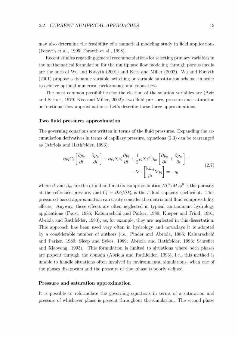
2.2. CURRENT NUMERICAL APPROACHES 13
may also determine the feasibility of a numerical modeling study in field applications
(Forsyth et al., 1995; Forsyth et al., 1998).
Recent studies regarding general recommendations for selecting primary variables in
the mathematical formulation for the multiphase flow modeling through porous media
are the ones of Wu and Forsyth (2001) and Kees and Miller (2002). Wu and Forsyth
(2001) propose a dynamic variable switching or variable substitution scheme, in order
to achieve optimal numerical performance and robustness.
The most common possibilities for the election of the solution variables are (Aziz
and Settari, 1979, Kiss and Miller, 2002): two fluid pressure, pressure and saturation
or fractional flow approximations. Let’s describe these three approximations.
Two fluid pressures approximation
The governing equations are written in terms of the fluid pressures. Expanding the ac-
cumulation derivatives in terms of capillary pressure, equations (2.3) can be rearranged
as (Abriola and Rathfelder, 1993):
φρlCl
[∂po
∂t− ∂pw
∂t
]+ φρlSlβl
∂pl
∂t+
1
2ρlSlφ
0βm
[∂po
∂t+
∂pw
∂t
]−
−∇ ·[kkrl
µl
∇pl
]= −ql
(2.7)
where βl and βm are the l-fluid and matrix compressibilities LT 2/M ,φ0 is the porosity
at the reference pressure, and Cl = ∂Sl/∂Pc is the l-fluid capacity coefficient. This
pressured-based approximation can easity consider the matrix and fluid compressibility
effects. Anyway, these effects are often neglected in typical contaminant hydrology
applications (Faust, 1985; Kaluarachchi and Parker, 1989; Kueper and Frind, 1991;
Abriola and Rathfelder, 1993), as, for example, they are neglected in this dissertation.
This approach has been used very often in hydrology and nowadays it is adopted
by a considerable number of authors (i.e., Pinder and Abriola, 1986; Kaluarachchi
and Parker, 1989; Sleep and Sykes, 1989; Abriola and Rathfelder, 1993; Schrefler
and Xiaoyong, 1993). This formulation is limited to situations where both phases
are present through the domain (Abriola and Rathfelder, 1993), i.e., this method is
unable to handle situations often involved in environmental simulations, when one of
the phases disappears and the pressure of that phase is poorly defined.
Pressure and saturation approximation
It is possible to reformulate the governing equations in terms of a saturation and
pressure of whichever phase is present throughout the simulation. The second phase

14 CHAPTER 2. LITERATURE REVIEW
pressure can then be removed from the equations by expressing it in terms of the
saturations and pressures of the other phase, using equations (2.4) and (2.5) the system
(2.3) is:
φ∂Sw
∂t−∇ ·
[kkrw
µw
(∇po −∇Pc)
]= −qw
−φ∂Sw
∂t−∇ ·
[kkro
µo
∇po
]= −qo (2.8)
The importance of this method is its suitability for problems where one fluid com-
pletely saturates the medium and the other one disappears. In the formulation of
equations (2.8) this would mean So = 0, because So does not appear explicity. The
pressure-saturation formulation has been employed by several authors (Faust, 1985;
Kueper and Frind, 1991a and 1991b; Forsyth et al. 1995; Binning and Celia, 1999).
Fractional flow approximation
This approach is motivated almost exclusively by the petroleum reservoir simulation.
One of its main characteristics is that it is necessary to formulate streamline simulators.
The basic idea of the fractional flow definition, fw, is to treat the total multiphase flow
as a single mixed fluid, and then describe individual phases through fractions of the
total flow,
fw =| uw || uT |
(2.9)
Total flux uT , can be defined as the sum of the phase volumetric fluxes:
uT = uw + uo (2.10)
Under the assumption that fluids are incompressible, if (2.4) and (2.10) are applied
to (2.1), divergence of total Darcy’s velocity is obtained:
∇ · uT = −(qo + qw) = −qT (2.11)
In one dimesion this equation has the particularly simple solution that the total flux
is constant in space and it is determined by boundary conditions.
P is the total (or global) fluid pressure. It is defined as the pressure that would
produce the flow of a fluid of a mobility (krl/µl) equal to the sum of the flows of fluids
w and o,
uT = −k
(krw
µw
+kro
µo
)∇P (2.12)

2.2. CURRENT NUMERICAL APPROACHES 15
the use of this variable reduces the coupling between pressure and saturation equations.
With these definitions the water flux can be expressed as a function of the total
flux with the help of the fractional flow function:
uw = uT fw (2.13)
Using this formulation (2.13), the mass-balance equation (2.1) for the water can be
expressed as:
φ∂Sw
∂t+∇ · (uT fw) = −qw (2.14)
developing the second term,
φ∂Sw
∂t+ uT · ∇fw + fw∇ · uT = −qw
Substituting the equation (2.11) and assuming that fw is function of saturation
(∇fw = dfw(Sw)dSw
∇Sw), equation for the two-phase flow in function of the fractional flow
is:
φ∂Sw
∂t+ uT ·
∂fw
∂Sw
∇Sw = fwqT − qw (2.15)
Total Darcy’s velocity uT is derived from the solution to the total pressure field (equa-
tion (2.10)).
This approach leads to two equations: a saturation equation (2.15), that is parabolic
for Sw and it has an advection diffusion form, and a global pressure equation ((2.10)
and (2.12)) whose form is elliptic for P . The advective term is nonlinear and usually
leads to shock formations.
Examples about the use of this approximation can be found in Douglas (1983),
Morel-Seytoux and Billica (1985a y 1985b), Dahle et al. (1990) Wagen (1993), Langlo
and Espedal (1994) and Chen et al. (1995). The principal drawbacks of the fractional
flow approach are: complex to be applied in three dimensions, poor performance for
general boundary conditions, and difficult performance in more general problems in-
volving heterogenous material properties (Binning and Celia, 1999). On the contrary,
the great advantage is its low computational costs.
2.2.2 Numerical approximation
Numerical simulation of multiphase flow, expressed with any of the mentioned appro-
ximations, can be performed with several techniques:
• Finite differences: This is the method addopted in this dissertation, so it
will be explained in detail along next chapter. Examples of its applications are

16 CHAPTER 2. LITERATURE REVIEW
Abriola (1985), Morel-Seytoux and Billica (1985), Faust (1985) and Kueper and
Frind( 1991).
• Finite elements: It overcomes the difficulties in the treatment of complicated
geometry and boundary conditions. It has been applied by a high number of
authors like Li et al. (1990), Schrefler and Xiayong (1993) Forsyth et al. (1995),
Chen et al. (1995) and Kim et al. (1996)).
• Techniques based on the characteristics method for the saturations
equation: This method is used when the equations are expressed in function of
fractional flow (Douglas, 1983; Dahle et al., 1990; Langlo and Espedal, 1994).
• Streamline simulators: Streamline based methods have received significant
attention over the last years. Nowadays they are accepted to be an effective
and complementary technology to more traditional flow modeling techniques as
finite differences and finite elements. A comprehensive review of the theoretical
basis for streamline simulation technology can be found in Batycky (1997) and
Thiele (2001). The key principles are to express the mass conservation equation
in terms of the time of flight and to reproduce the 3D solution by combining one
dimensional solutions along streamlines. One benefit of streamline simulators
is its inherent memory and computational efficiency, being for many problems
2 to 3 order of magnitude faster than conventional finite difference simulators.
Applications of streamline simulators in different cases have been performed by
Batycky and his team (e.g., Batycky et al., 1996a and 1996b; Batycky, 1997).
Several works comparing the different behavior of the different approaches can
be found in the literature. Young (1984) compares the sensitivity to the grid size
and orientation. Ewing (1991) reviews numerical techniques for the solution of the
pressure equations in the fractional flow approach, and demonstrates the importance
of accurate determination of velocities. Abriola and Rathfelder (1993) analyse the mass
balance errors, and Binning and Celia (1999) study the advantages and disadvantages
of the characteristics method. Recently, the control volume finite element method and
the control volume function approximantion (Li et al., 2003) have been developed to
enforce the conservation property and get accurate fluid velocities using finite element
methods.
For temporal discretization there are also several choices, being the fully-implicit
time stepping the dominant approach in hydrology, while in traditional petroleum
engineering literature the predominant approach is the explicit or semi-explicit.
Anyway, it should be pointed out that a non mass conservative numerical scheme
may still give accurate and correct solutions with mass conservative results as long as

2.3. INVERSE STOCHASTIC SIMULATION 17
both spatial and temporal discretization are sufficiently small. A mass conservative
solution may not guarantee the accuracy of the solution. In other words, the ability
of a numerical model to conserve mass is a necessary but no sufficient condition for
convergence (Cella et al., 1990).
When the working scale is large a great computational time is required. There has
been a huge advance in new computational algorithms for solving the problem faster
and with better discretization. This fact, and the extraordinary advances in computer
hardware have resulted in quite good algorithms and codes that allow to perform fairly
efficiently the multiphase flow simulation. Although, it is always desirable to obtain
more speed and capacity for computing to achieve better model discretization and
characterization. Consequently, numerical simulation of multiphase flow remains a
challenging task. In Wu et al. (2002) there is a review of the last advances, and the
presentation of a new technique that allows to improve the compute efficiency with the
parallel-computing method (Larsen and Bech, 1990).
2.3 Inverse stochastic simulation
2.3.1 Stochastic framework
Until the eighties decade, most reservoir descriptions employed in simulation models
consisted of a layered system, where along each layer the petrophysical and flow pro-
perties (permeability, porosity, dispersivity, etc.) were homogeneous. This view of
modeling a reservoir suffered a major revolution with the recognition that it can be
impossible to characterize the natural variability in a deterministic way (Freeze, 1975).
This natural heterogeneity of the medium properties affects significantly the flow beha-
vior through porous media (i.e., Miller et al., 1998 and its references). Unfortunately,
it is quite difficult to characterize the heterogeneity of the different properties because
they are sampled at few locations, they are defined at laboratory scale, and they must
be specified at every location represented in the numerical model by smooth interpo-
lating the data at sampled locations. For example, porosity is generally less variable
than permeability, and can be measured fairly directly by well logging or experiments
on reservoir core samples, but permeability is much more heterogeneous, and difficult
to measure.
Stochastic analysis revealed to be a method that permits to model the spatial varia-
bility of heterogeneous hydraulic properties, by a space random function characterized
by its multivariate distribution (Matheron, 1973; Freeze, 1975; Smith, 1981; Hoeksema
and Kitanidis, 1985a; Dagan, 1986; Sudicky, 1986). In the stochastic framework, with
a few selected statistical parameters of the subsurface properties such as mean and
18 CHAPTER 2. LITERATURE REVIEW
variance, the overall variability of the flow processes can be determine. Geostatistical
techniques provide efficient tools to generate equi-probable distributions of unknown
fields from sampled data.
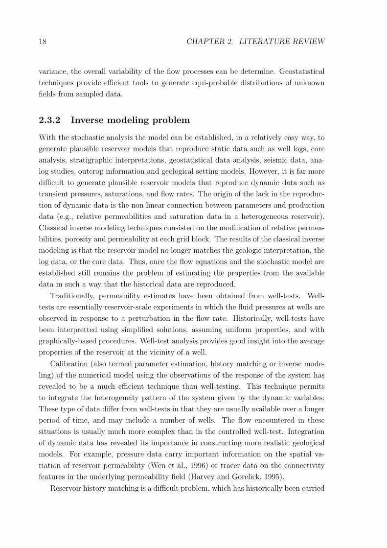
2.3.2 Inverse modeling problem
With the stochastic analysis the model can be established, in a relatively easy way, to
generate plausible reservoir models that reproduce static data such as well logs, core
analysis, stratigraphic interpretations, geostatistical data analysis, seismic data, ana-
log studies, outcrop information and geological setting models. However, it is far more
difficult to generate plausible reservoir models that reproduce dynamic data such as
transient pressures, saturations, and flow rates. The origin of the lack in the reproduc-
tion of dynamic data is the non linear connection between parameters and production
data (e.g., relative permeabilities and saturation data in a heterogeneous reservoir).
Classical inverse modeling techniques consisted on the modification of relative permea-
bilities, porosity and permeability at each grid block. The results of the classical inverse
modeling is that the reservoir model no longer matches the geologic interpretation, the
log data, or the core data. Thus, once the flow equations and the stochastic model are
established still remains the problem of estimating the properties from the available
data in such a way that the historical data are reproduced.
Traditionally, permeability estimates have been obtained from well-tests. Well-
tests are essentially reservoir-scale experiments in which the fluid pressures at wells are
observed in response to a perturbation in the flow rate. Historically, well-tests have
been interpretted using simplified solutions, assuming uniform properties, and with
graphically-based procedures. Well-test analysis provides good insight into the average
properties of the reservoir at the vicinity of a well.
Calibration (also termed parameter estimation, history matching or inverse mode-
ling) of the numerical model using the observations of the response of the system has
revealed to be a much efficient technique than well-testing. This technique permits
to integrate the heterogeneity pattern of the system given by the dynamic variables.
These type of data differ from well-tests in that they are usually available over a longer
period of time, and may include a number of wells. The flow encountered in these
situations is usually much more complex than in the controlled well-test. Integration
of dynamic data has revealed its importance in constructing more realistic geological
models. For example, pressure data carry important information on the spatial va-
riation of reservoir permeability (Wen et al., 1996) or tracer data on the connectivity
features in the underlying permeability field (Harvey and Gorelick, 1995).
Reservoir history matching is a difficult problem, which has historically been carried

2.3. INVERSE STOCHASTIC SIMULATION 19
out with trial and error processes. Nowadays the automatic history matching is used
to achieve a solution to the inverse problem. Automatic inverse modeling is based on
minimizing an objective function, J , which includes a sum of squared production data
mismatch terms:
J =Ts∑t=1
Ns∑i=1
ws,i(SSIMi,t − SMEAS
i,t
)2+
Tp∑t=1
Np∑i=1
wp,i
(pSIM
i,t − pMEASi,t
)2(2.16)
Ns and Np are, respectively, the number of saturation and pressure measured points.
Ts and Tp are, respectively, the number of times in which saturation and pressure are
measured, and the indexes SIM and MEAS are referred to simulated and measured
values. ws,i and wp,i are weighting terms.
Minimization is done based on least squares methods (linear or non linear multiple
variable regression) or optimization routines, which due to the non linearity of the
parameters requires the usage of iterative processes.
One of the first works presented for automatic history matching was the one of
Jacquard and Jain (1965). They applied the gradient method to the estimation of
permeability in a two dimensional reservoir from pressure data obtained under single-
phase flow conditions. They based their procedure on the computation of sensitivity
coefficients, using an electric-circuit analog, and used zonation to limit the number
of parameters to be estimated. Later, motived by Jacquard and Jain’s ideas, Carter
et al. (1974) presented a derivation of the method to compute sensitivity coefficients
for two dimensional single-phase flow problems. This procedure can be applied to
compute sensitivity of simulator grid block pressures to all grid block permeabilities
and porosities. Despite their efficiency, these initial studies are limited by the fact that
they are restricted to linear problems and consequently are not applicable to multiphase
flow problems.
2.3.3 Ill-posedness
The minimization problem is said to be ill-posed as its solution does not guarantee the
following properties (Carrera and Neuman, 1986a; Sun, 1994):
• Existence: The observation error (or noise) of state variables cannot be avoided.
As a result, an accurate solution of the inverse problem may not exist.
• Uniqueness: Different combinations of hydrogeologic conditions may lead to
similar observations of production variables. Hence, it is impossible to uniquely
determine the particularities of the reservoir by only observing the state variables.

20 CHAPTER 2. LITERATURE REVIEW
• Stability: Instability frequently results due to poor degree or lack of one-to-one-
ness in the pertinent operator. This feature produces a flat objective function
surface around minima.
For example (Watson et al., 1994), the estimation of the absolute permeability k(x)
(equation (2.2)) from pressure data taken at a well p(x0, t). The estimation of k(x) in
two or three dimensions cannot be appropriately done from the one dimensional data
p(x0, t). This feature results in non uniqueness in the solution. It is also possible that
no minimum of the objective function exists, or that two different sets of k give two
different p(x0, t) which are close. This makes inversion to be unstable.
In order to mitigate or eliminate these problems more information, apart from the
state variable observations, can be used. The technique known as regularization is a
way of alleviating the ill-posedness of inverse problems through the incorporation of
prior constrains or information into the objective function (Sun, 1994). Carrera and
Neuman (1986a, 1986b and 1986c) used prior information to modify the likelihood
function and showed that the use of prior information reduces the ill-posedness of the
problem. In this sense, the introduction of prior data is similar to a regularization of
the ill-posed problem as reduces the non uniqueness, but also reduces the instability
in the computational algorithms (Chu et al., 1995).
2.3.4 Optimization algorithms
There are a number of strategies to find parameter combinations that yield smaller
values of the objective function, eventually identifying a local or hopefully global mi-
nimum. The available algorithms can be classified as follows (Sun, 1994):
• Search methods: In this kind of methods the objective function is evaluated
for different parameter combinations, mapping out the objective function in the
n-dimensional parameter space, looking for the minimum. While no derivatives of
the objective functions with respect to the parameters must be calculated, these
methods usually require many function evaluations and are therefore inefficient.
Examples of search methods include trial-and-error, Fibonacci section search,
golden section search and quadratic interpolation method. Detailed discussions
about these methods can be found in any textbook on numerical optimization
(e.g., Scales, 1985).
• Gradient based methods: For this set of methods it is required the calculation
of the gradient of the objective function with respect to the parameter vector,
along the direction given by the gradient. The procedure is robust, but time ex-
pensive. The basic gradient method is steepest descent method, which uses the

2.3. INVERSE STOCHASTIC SIMULATION 21
negative gradient direction as the search direction in each iteration. However,
steepest descent usually terminates far from the solution due to round-off effects.
Instead, a conjugate gradient method as the one of Fletcher and Reeves allows to
find the minimum more efficiently (Carrera and Neuman, 1986b). For conjugate
gradient methods the computational requirement for each iteration is relatively
low, but the number of iterations required can be large, especially for multiphase
flow problems (Makhlouf et al., 1993). Other possibility is the adjoint method,
which is very efficient because the flow problem and the adjoint sensitivity pro-
blem have the same form, hence the calculation of the sensitivity coefficients is
straightforward. The adjoint method has also been applied to multiphase flow
problems, altough in many cases it resulted to be high computationally cost.
Carrera and Neuman (1986b) studied the convergence when switching from one
method to another when the former slows down or fails to convergence. Their
conclusion is that changing the optimization algorithm, an improvement in the
rate of convergence can be obtained.
• Second order methods: When the method is based on the Hessian matrix,
instead of the gradient, the approach is known as second order method. The com-
putational cost of calculating the second derivatives is compensated with a rat-
her efficient stepping in the parameter space. Examples of second-order methods
are Newton method, Gauss-Newton method and Levenberg-Marquardt method.
Standard implementations of these algorithms require calculation of sensitivity
coefficients, which formally represents the derivative of predicted variables with
respect to the model parameters. An excellent review of methods for computing
sensitivity coefficients and solving inverse problems was presented by Yeh (1986).
Chu et al. (1995) presented an efficient method of computing sensitivity coeffi-
cients. Additional information can be incorporated when it becomes available.
This method yields a smoothed version of the true distribution. Wu et al. (1999)
presented a good review about the calculation of sensitivity coefficients, and de-
veloped an algorithm to use the adjoint method to get the sensitivity matrix for a
two-phase flow problem, in a way that the Gauss-Newton method can be used for
inverse modeling. The drawback is that the adjoint approximation needs storage
of pressures and saturations for all the nodes and times of discretization. There
exist analytical developments of sensitivity parameters for the multiphase flow
like the ones of Ates and Kelkar (1998) or Vasco et al. (1999). Applications of
Gauss-Newton method and the calculation of sensitivity coefficients in the inte-
gration of well-test information, production history and time-lapse seismic data
can be found in the work of Landa (1997 and 2001).

22 CHAPTER 2. LITERATURE REVIEW
• Heuristic methods: The most common are simulated annealing (Hegstad et
al., 1994) or genetic algorithms (Romero et al., 2000). These methods sample a
much larger solution space than gradient methods and increase the likelihood of
obtaining global minimums to the objective function. However, their convergence
is reached quite slowly.
2.4 Inverse modeling methods
Depending on the assumptions taken, the optimization algorithm, the way the para-
meters are estimated, or the strategy for inversion, there are many different kind of
methods for inversion. The most extended methods are the ones that calibrate pertur-
bing non calibrated realizations of the model. For this type of methods the efficiency
depends on the way realizations are perturbated. For an extensive and comprehen-
sive review about the existing methods for integration of production data in reservoir
models, it is recommended to look at Wen et al. (1997), Oliver et al. (2001) or
Hendricks-Franssen (2001), and the references contained therein. In this section it is
presented a brief resume of the principal methods, developed until present time, that
integrate dynamic variables through inverse modeling. In Zimmerman et al. (1993)
there is a complete study comparing some of the inverse approaches described here.
The main conclusion achieved on this study was the importance of the appropriate
selection of the variogram and the time and experience devoted by the user of the
method in analyzing and modeling the observed data.
2.4.1 Cokriging method
Cokriging is a geostatistical tool for estimating two or more random fields together
by using their measurements, when they are correlated. This method was applied to
inverse groundwater modeling by Dagan and Rubin (Dagan, 1985; Rubin and Dagan,
1987a; Rubin and Dagan 1987b; Dagan and Rubin, 1988) and Hoeksema and Kitani-
dis (Hoeksema and Kitanidis, 1984; Hoeksema and Kitanidis, 1985b). The unknown
transmissivity value at a point is estimated by a weighted linear combination of the
observed transmissivity and pressure. Dagan (1985) and Rubin and Dagan (1987b)
showed that when the random transmissivity and pressure fields are jointly Gaussian
with known mean and covariance, the cokriging estimate and cokriging covariance are
equivalent to the conditional mean and conditional covariance of the new joint probabi-
lity distribution function conditioned on the measurements. The statistical parameters
are estimated by the maximum likelihood method that includes linearizations of the
steady state flow equations. Analytical expressions of cross-covariances of permeabi-

2.4. INVERSE MODELING METHODS 23
lity and pressure are obtained assuming uniform flow and infinite domain. Harvey
and Gorelick (1995) have applied the cokriging method to flow and tracer transport
integrating tracer arrival time data, concluding that it improves the accuracy of the
permeability estimation.
As transmissivity and pressure are non linearly related, the classical cokriging met-
hod needed a modification. To overcome this problem Yeh et al. (1996) proposed
an iterative stochastic inverse method to estimate transmissivity and pressure fields
that account for transmissivity and pressure data. It first estimates a transmissivity
field by cokriging from the available transmissivity and steady state pressure data.
The flow equation is then solved numerically to obtain a pressure field. The cova-
riance and cross-covariance of transmissivity and pressure are then updated and a new
transmissivity field can be obtained by again cokriging using the updated covariance
and cross-covariance. This process is continued until the variance of estimated trans-
missivity stabilizes. Later the method has been changed in the sense that a Monte
Carlo simulation approach is adopted (Hanna and Yeh, 1998) to account for the mass
conservation of the approach. The method requires significant computational effort,
while its advantages are that it is very simple to implement and has not suffered from
convergence problems.
2.4.2 Fast Fourier transform method
This method was developed by Gutjahr (Gutjahr, 1989; Gutjahr et al., 1993), and
allows to condition to both transmissivity and pressure data by using linearization and
fast Fourier transform method. The covariance and cross-covariance are represented
as functions of the spectral and cross-spectral density. Transmissivity realizations
conditioned to the pressure data are constructed by adding the difference between
the unconditional simulation and kriged values of the unconditional simulation to the
kriged values using the field data. The key assumption is the linearized flow equation
as in the linearized cokriging method. Later this method has been extended to account
for the non linear relationship between transmissivity and pressure in the computation
of the pressure covariance and the pressure-transmissivity cross-covariance using an
iterative approach (Gutjahr et al., 1994). This technique is very efficient and is capable
to generate many realizations with modest computing resources over times on the order
of minutes.

24 CHAPTER 2. LITERATURE REVIEW
2.4.3 Pilot point method
The pilot point method (de Marsily et al., 1984) reproduces pressure data by calibrating
the transmissivity field. The method starts by generating a conditional simulation
of the transmissivity field with geostatistical techniques. Then, the generated field
is modified by adding other transmissivity data at some select locations (called pilot
points). Adjoint sensitivity analysis is used to determine the locations where additional
transmissivity data should be included in order to improve the reproduction of the
pressure data. The new transmissivity data at the selected pilot points are treated as
local data, a new conditional realization of transmissivity is then generated, and, the
flow model is run again. The iteration of adding pilot points is continued until a least-
squared error criterion is met or the addition of more pilot points does not improve the
calibration. One of the disadvantages of this method is that is very CPU intensive.
Lavenue and Pickens (1992) and Ramarao et al. (1995) applied the pilot point
method to reproduce pressure data. In their work, they generated a selected number
of conditionally simulated transmissivity fields and calibrated each of the fields to
reproduce the pressure data.
2.4.4 Self-calibrated method
This method is also an iterative geostatistical based inverse technique, which reduces
the parameter space to be estimated in the optimization process. The conditioning to
pressure is done by solving the groundwater flow equation, not through any lineariza-
tion. It was introduced by Sahuquillo et al. (1992), and developed later by Gomez-
Hernandez and others (Gomez-Hernandez et al.,1997; Capilla et al., 1997; Capilla et
al., 1998). It was the first inverse stochastic simulation method to construct multiple
equiprobable transmissivity fields honoring single-phase historical pressure data.
In the self-calibrated method the spatially variable transmissivity values are para-
meterized as the sum of a seed transmissivity field, obtained by standard geostatistical
techniques, plus a perturbation of the entire field, which is expressed as a linear func-
tion of the perturbations at a selected number of locations referred to as master blocks.
This approach can also account for uncertainty in flow boundary conditions (pressure
or flowrate).
The self-calibrated method basic ideas and numerical schemes will be addopted in
this dissertation for the development of a two-phase inverse modeling method, therefore,
more details about the self-calibration method can be found in the following chapters.
In Wen et al. (1998) the self-calibrated method was extended to integrate pro-
duction data, such as fraction flow rate data and pressure at production wells. To

2.4. INVERSE MODELING METHODS 25
reach this aim a streamline based multiphase flow simulator was adapted for fast flow
simulation. One dimensional single-phase analytical streamline solution was utilized
for fast calculation of fractional flow sensitivity coefficients.
The self-calibrated method has also been extended by Hendrics-Franssen (2001) to
handle transient groundwater flow, joint conditioning of transmissivity and storativity
fields, and to couple inverse modeling of groundwater flow and mass transport (the
objective function also includes the mismatch corresponding to concentration data).
An application of the self-calibrated method to two-phase flow has been presen-
ted by Wen et al. (2002), using multiphase production data to estimate the spatial
distribution of lithofacies in 2D.
2.4.5 Maximum likehood method
This is a general non linear technique that estimates reservoir parameters using prior
estimates along with transient or steady state pressure data. Early development of this
method was presented in a series of three papers of Carrera and Neuman (Carrera and
Neuman, 1986a; Carrera and Neuman, 1986b; Carrera and Neuman, 1986c). Parameter
estimation is performed using the maximum likelihood theory, incorporating the prior
information into the likelihood function. The non linear flow equation is solved by a
numerical method.
The likelihood function expresses how likely are the parameteres to have producted
the observed data. The method of maximum likelihood consists of finding the specific
value of the parameter that is most likely to have produced the data. The inverse
problem solution is obtained iteratively. The most important characteristic of the
method is that aquifer parameters are estimated for a limited number of zones which
partition the aquifer. Different parameteres can be estimated for each zone such as,
values and directions of principal hydraulic conductivities in anisotropic media, specific
storage, boundary conditions, or recharge rates. This method is also computationally
intensive in the optimization process.
2.4.6 Markov Chain Monte Carlo Method
In the Bayesian approach, parameters are taken as random and through the differential
equation the state variables are also random, yielding the same results as conceptua-
lized from the geostatiscal approach. The method has been proposed by the team at
the Norwegian University of Science and Technology to integrate historical production
data (Hegstad et al., 1994; Omre and Tjelmeland, 1997; Tjelmeland and Omre, 1997;
Hegstad and Omre, 1997). This team was one of the pioneers in the applications of

26 CHAPTER 2. LITERATURE REVIEW
Markov chain Monte Carlo methods to the earth science for generating realizations
from a specified (but unnormalized) probability density function in reservoir characte-
rization. Inspired by their work, Oliver and others (Oliver et al., 1996; Oliver et al.,
1997) employed the Markov chain Monte Carlo method for the generation of reservoir
models that are conditional to transient pressure data. The most probable model (the
maximum a posteriori estimate) conditioned to both prior information and pressure
data is obtained by minimizing an objective function derived directly from the a poste-
riori probability density function. The decision to accept or reject the resulting history
matched realization is made on the basis of the Metropolis-Hastings algorithm. As in
most of the methods mentioned until this point, with the exception of the fast Fourier
method, in many applications the computational demands of the simulator can greatly
restrict the number of forward simulations that can be carried out. Consequently, the
Markov chain Monte Carlo method is hard, or even impractical, to implement. One
way to overcome this difficulty is to us the multi-scale computational model. Slightly
following the ideas suggested by Celia et al. (1993), Higdon et al. (2002) speed up the
forward simulator by running it on a smaller, coarsened version of the original inputs.
Then, use the resulting posterior simulation output to guide and speed up the posterior
simulation on the original, fine-scale specification.
2.4.7 Simulated annealing method
Simulated annealing has its basis in statistical theory, being a flexible and generally
applicable heuristic optimization technique (Hegstad et al., 1994). It does not require
neither a functional form for the covariances, nor gradient calculations. A perturbation
is applied in a set of grid blocks and an energy objective function is evaluated. The
decision of wether accepting or not the perturbation is based on the change of energy
caused by this perturbation. Its extensive use arises from the fact that additional data
constraints can be incorporated by a simple modification of the objective function
and its success in generating parameter fields that give a good approximation to the
global minimum of the objective function. The computational costs become immense
if the objective function includes production data that must be generated at each
iteration by solution of a forward problem using a reservoir simulator. It belongs to
the class of Markov chain Monte Carlo techniques, but when it is used without careful
consideration of the stopping temperature, the results will not be random realizations
from the correct probability density function.
Datta-Gupta et al. (1995) were able to use the simulated annealing method to
generate stochastic permeability fields conditioned to both spatial statistics and tracer
data. They also applied it to water-oil displacement calculations. Several examples of

2.4. INVERSE MODELING METHODS 27
simulated annealing usage for estimating model parameters in order to solve remedia-
tion management problems are provided in Finsterle and Pruess (994).
2.4.8 Genetic Algorithms
In the same way that simulated annealing is applied to address the optimization pro-
blem, the genetic algorithms have been used for reservoir engineering in several works,
including those by Romero et al. (2000), Romero et al. (2000b) and Romero and
Carter (2001). Genetic algorithms are a class of optimization methods which draw
on ideas from natural evolution and genetics. They are randomized search algorithms
based on an analogy to the mechanics of natural selection according to the Darwinian
evolutionary theory and the survival of the fittest principle. In the case of Romero et
al. (2000) and Romero and Carter (2001) the genetic algorithms has been applied to
optimize the inversion problem in which the pilot points method (de Marsily et al.,
1984) is used. Like the simulated annealing method the genetic algorithm has a slow
rate of convergence and is computationally inefficient. The main attractions of simula-
ted annealing and genetic algorithm formulations are their simple integration of static
data and their ability to converge to the global minimum of the objective function
whereas in the gradient based methods it is common to end up in a local minima or a
saddle point.
2.4.9 Two-step inversion for multiphase flow
A two step inversion method was developed by Vasco et al., 1999. This method utilizes
a multiphase streamline simulator as a forward model. The parameter sensitivities
are formulated in terms of one dimensional integrals of analytic functions along the
streamlines. The integration of dynamic data is then performed using a two-step
iterative inversion: (1) match the breakthrough times at the producting wells and (2)
matching the production history. The pressure and streamlines are recalculated for each
iteration during inversion. The approach follows from an analogy between streamlines
and ray tracing in seismology. One advantage is that sensitivities for all the reservoir
parameters require a single simulation. Yoon et al. (1999) have extended this approach
to multiscale, relying on a hierarchical parameterization and a scale-by-scale inversion
of the production response. With this extension, they are able to account explicitly for
varying data resolution.
Another two-step approach was presented by Wang and Kovscek (2000). However,
their method does not compute sensitivity coefficients nor is their formulation of the
inverse problem similar to Vasco et al’s approach. Their basic idea is to relate the

28 CHAPTER 2. LITERATURE REVIEW
fractional flow curve at a producer to the water breakthrough of individual streamlines.
By adjusting the effective permeability along streamlines, the breakthrough time of
each streamline is found that reproduces the reference producer fractional-flow curve.
The second step is to map the streamline permeability modification onto the grid blocks.
Then, flow simulation is performed to check the match and the process is iterated until
convergence. Argarwal and Blunt (2001) have extended the method proposed by Wang
and Kovscek (2000) to compressible models with gravity. However, Argawal and Blunt
(2001) consider gravity and compressibility only for the forward streamline simulator,
and do not take them into account to find the permeability perturbation.
2.4.10 Gradual Deformation
Developed very recently (Roggero and Hu, 1998; Hu, 2000a; Le Ravalec-Dupin, et al.,
2000), gradual deformation is a parameterization method that reduces considerably
the unknown parameter space of stochastic models. The method is based on the fact
that linear combinations of multi-Gaussian random functions remain multi-Gaussian
random functions. It consists in iteratively optimize combinations of independent rea-
lizations of a stochastic model until the constrains are satisfied. This method, initially
developed for Gaussian stochastic models, has been extended to non Gaussian realiza-
tions (Hu, 2000b).
The gradual deformation method has been developed by combining independent
realizations, the different features of the procedure using dependent realizations have
been recently analyzed by Hu (Hu, 2002). This new formulation improves the nu-
merical stability of the method, at the same time that explicitly takes into account
the numerical dependence between realizations, allowing the deformation of conditio-
nal realizations. However, this procedure is limited to global deformations with fixed
structural parameters. The modification of the gradual deformation algorithm made
by Ying and Gomez-Hernandez (2000) allows to honor the well data while preserving
the permeability variogram. In the paper mentioned above by Wen et al. (2002), Ying
and Gomez-Hernandez’s algorithm is modified to invert lithofacies distribution from
production data within the framework of truncated Gaussian simulation.
2.4.11 Fractal simulation method
This method treats the spatial distribution of reservoir permeability as fractal (Grin-
drod and Impey, 1993). The fractal parameters are estimated from field data (per-
meability and pressure) by maximum likelihood estimation method. Reservoir models
conditional to the pressure data are constructed through a linear superposition of un-

2.5. UNCERTAINTIES 29
conditional fields, as in the linearized fast Fourier transform method with randomly
generated phase and amplitude coefficients. A linear superposition of the unconditio-
ned fields is used to condition them to observed data, minimizing the difference between
the variance of the final field and the data.
2.4.12 Neural networks
Artificial neural networks can be trained to predict the outcome of the flow code. For
example, Rogers and Dowla (1994) trained an artificial neural network to predict the
mass of contaminant removed during 50-year simulation period, and then they used the
neural network to optimize a groundwater remediation plan. The principal advantage
that this technique gives for history matching is its potential to be implemented in
parallel processes in order to improve the speed of flow simulations.
2.5 Uncertainties
Having defined the parameters to be used in the reservoir model, the way to minimize
the objective function and the inversion approach, the result is a reservoir model which
is conditioned to both static and dynamic data. This model is then used to forecast
the future behavior of the reservoir. Traditional inversion techniques result in a single
best reservoir model that minimize the differences between the observed and simulated
historical data. But this prediction is affected by errors or uncertainties, as the error in
the input parameters lead to errors or uncertainties in the model predictions. Integra-
tions of additional data reduces the uncertainty of the model (Wen et al., 1998), but
the resulting best model is usually oversmooth compared to the real reservoir. either
this parameter uncertainty at unsampled locations is quantified. When using the re-
servoir model for prediction, the next step is to quantify the forecast uncertainty. The
purpose of inverse modeling is not only to estimate best parameters for a given model
structure, but also to reduce and estimate the parameter uncertainty.
Uncertainty quantification in the dynamic reservoir modeling is one of major cha-
llenges facing reservoir modeling. There are mainly two approaches to quantify the
flow-prediction uncertainty using the simulation methods described.
One of the methods to solve this problem is the Monte Carlo approach. This
method, as it has been explained in the section above, consists in performing a high
resolution flow simulation for each of a large number of realizations of the reservoir
description. It is based on the fact that the resultant distribution is an equal likely
representation. The dependent variables are averaged over many realizations to ob-
tain statistical moments, or probability distribution functions of the model prediction.

30 CHAPTER 2. LITERATURE REVIEW
Since it is a statistical postprocessing of deterministic flow simulations, the Monte Carlo
simulation approach is flexible. However, because of computational expense, someti-
mes it can be very difficult to generate sufficient conditional realizations to evaluate
uncertainty. Often, only few realizations are generated; for example, in the PUNQ
(production forecast uncertainty quantification) study, comparing several uncertainty
quantification methods for production forecasting, most participants generated 10 rea-
lizations (Floris et al, 2001). Another drawback of the Monte Carlo approach is that
the ensemble of realizations could provide a poor representation of uncertainty because
of a defect in the model or the sampling algorithm. The advantages are that any dis-
tribution function can be chosen, the non linearities are taken into account and the
results have a physical meaning.
One class of Monte Carlo techniques is the Markov chain Monte Carlo method
(Hegstad and Omre, 1997), which has been explained before. In Hegstad and Omre
(1998) an application to that approximation was shown and in Omre (2002) several
algorithms for the sampling of the posterior model were presented. One of that algo-
rithms to estimate the uncertainty of the model predictions is described in Oliver et al.
(1996) and Oliver et al. (1997), employing the Markov chain Monte Carlo technique
to generate a set of realizations. In Oliver’s approach a sample is drawn from the
prior reservoir model. Concurrently, a sample is also drawn from the production data.
This production sampling is done because the production data contains observation
errors and the reservoir model contains modeling error. Pairs of prior reservoir sam-
ples and production samples are subsequently history matched. The matching criterion
is formed by both the mismatch between the production sample and the simulated pro-
duction data and the deviation of the reservoir model from the sampled prior reservoir
model used as starting point for the optimization. Applications of Oliver’s approach
to full-field reservoir problems can be found in Wu et al. (1999) and Floris and Bos
(1998).
As it has been mentioned before the self-calibrated method (Sahuquillo et al., 1992;
Gomez-Hernandez et al., 1997; Capilla et al., 1997; Capilla et al., 1998; Hendrincks-
Franssen, 2201) was the first method to use inverse modeling techniques in the context
of generating multiple realizations. The self-calibrating method uses stochastic appro-
ximation to solve single-phase inverse flow problem. For example, in Gomez-Hernandez
et al. (1997) inverse modeling is applied to a number of stochastic reservoir models
and the range of forecasts is used as a quantification of uncertainty. In Ramarao et al.
(1995) there is an application of pilot point method and Monte Carlo techniques for
the quantification of uncertainty.
To avoid the computation of a high number of realizations, there is an alternative

2.6. RELATIVE PERMEABILITY 31
to the Monte Carlo methods, this technique consists in solving the statistical moment
equations of the interest variables (Zhang and Tchelepi, 1999; Zhang et al., 2000). The
stochastic differential equations that describe the flow process are averaged to obtain
the equations governing the statistical moments of the dependent variables. Then
the moment differential equations are solved either analytically or numerically. The
moment differential equations are commonly derived under the assumption that small
perturbation and with some kind of closure approximation. Zhang and Techelepi’s work
presents analytical solutions for simple 1D and 2D non linear problems, but is limited
to uniform mean flow in unbounded domains. Zhang et al. (2000) have extended the
Lagrangian statistical moment approach to more complex domains and flow patterns
due to the presence of wells. Huang et al. (1996) presented one of the first attempts to
quantify uncertainties for multiphase systems. They showed that secondary production
performance uncertainty is more affected by the iner-well variation of the permeability
field than primary production. Thus, descriptions obtained based on matching primary
performance are inadequate for secondary production performance matching. Other
studies as the one of Wen et al. (1998) have pointed out that the uncertainty is highly
influenced by the flux conditions of the system, for example the production state in
the wells.
To finish with the review about methods for estimation the parameter and model
uncertainties, gradual deformation method applications are analyzed. Le Ravalec et
al. (2000) presented a study proving that the realizations constructed with the gradual
deformation method do not reflect properly the posterior probability density function.
Hence, their conclusion was that the gradual deformation method cannot be used to
infer the uncertainty. At the same time, in this work it is proposed an improved gradual
deformation method. In this extension additional conditions for the objective function
were considered, allowing to investigate the conditioned realizations space from the
calibrated realizations, and then to obtained a measure for the uncertainty.
2.6 Relative permeability
History matching makes possible to build a reservoir model that satisfies static as well
as dynamic data. Integration of dynamic data centers its attention in the estimation
of absolute permeabilities. Relative permeability functions are generally estimated by
interpreting flow data collected from laboratory displacement experiments in which one
fluid is injected into a core sample that is saturated with another fluid or fluids. Typi-
cally the data consist of time dependencies of the differential pressure across the core
sample and the cumulative production of the fluid displacement. The interpretation
32 CHAPTER 2. LITERATURE REVIEW
of displacement data is usually based on the application of semi-analytical approa-
ches (Mitlin et al., 1999) or numerical simulations. The minimization of the objective
function in the semi-analytical method developed by Mitlin et al. (1999) is ensured
by using the simulated annealing method. They improved the model accounting for
presssure drop data before breakthrough in the laboratory experiments. Over the last
decade numerical inverse algorithms have been developed for the estimation of relative
permeabilities at core scale (Watson et al., 1994; Grimstad et al., 1997). Considerable
progress has been made in the methodology for interpretting core flow experiments
and recent experimental advances are providing exciting prospects for even more ef-
fective solutions on the laboratory scale. However, relatively little attention has been
directed to the estimation of these properties at reservoir scale. The values obtained in
the laboratory can be very different to the ones corresponding to the conceptual and
numerical model, mainly due to the scale effects (Frykman and Lindgaard, 1997) and
differences in reservoir conditions and laboratory conditions. In the study presented by
Smith (1991) the influence of heterogneities on average relative permeability functions
is analyzed. However, this study is performed for steady state conditions. Hastings
et al. (2001) presented a streamline simulator that permits to calculate multiphase
flow taking into account both heterogeneities of absolute and relative permeabilities
at reservoir scale. They apply the inverse method in order to calculate the uncertain-
ties of these parameters nor to the simultaneous estimation of absolute and relative
permeabilities. Alpak et al. (2001) is another of the few articles for the estimation of
two-phase relative permeabilities at reservoir scale. The problem of their application
to two-phase flow is that they use a single-phase inversion algorithm. Their idea was to
detect radial variability in the water saturation profile from the corresponding profile
of relative permeabilities.
During last years several works about the estimation of absolute and relative per-
meabilities with inverse techniques have been published (Watson et al., 1994; Kulkarni
and Datta-Gupta, 1999; Ates and Kelkar, 2000; Valestrand et al., 2001). In these works
different approaches are used, for different scales, but always considering homogeneous
relative permeability curves all over the study area. Kulkarni and Datta-Gupta (1999)
used the streamline based method developed by Vasco et al. (1999) to estimate re-
lative permeabilities from production data at reservoir scale for homogeneous relative
permeability curves. They concluded that the water front is highly sensitive to the
end-point water relative permeability. They also showed that water breakthrough data
are not sufficient to derive reliable estimates of both absolute and relative permeabili-
ties, and pressure information needs to be added. Valestrand et al. (2001) developed
an inverse method for simultaneous determination of absolute and relative permeabi-

2.6. RELATIVE PERMEABILITY 33
lities, but at core scale and for homogenous relative permeabilities. In their method
the relative permeabilities are estimated first by utilizing the harmonic mean value of
the absolute permeability. Then the absolute permeability is estimated, keeping the
relative permeabilities fixed at their first estimate. The procedure is repeated until
convergence. Some examples in 1D are presented.
Different analytical expressions have been developed for relative permeability cur-
ves. B-Splines (Kulkarni and Datta-Gupta, 1999; Valestrand et al., 2001) or potential
functions (Mitlin et al., 1999; Ates and Kelkar, 2000; Akin, 2001) are frequently used.
For this dissertation, the conventional Corey functional representations are used to
approximate water relative permeability, krw, and oil relative permeability, kro:
krw = k0rw
(Sw − Srw
1− Srw − Sro
)nw
(2.17)
kro = k0ro
(So − Sro
1− Srw − Sro
)no
k0rw and k0
ro are the end-point relative permeability curves, Srw and Sro the residual
saturations, and nw and no the shape exponents, for water and oil respectively.
Depending on which expressions for relative permeability curves are selected, the
parameters for the calibration change. For example, Ates and Kelkar (2000) used the
Corey function representations. They applied the method of the double loop (Ates and
Kelkar, 1998) for optimizing both relative and absolute permeabilities. They study the
sensibility of breakthrough with respect to the end-point relative permeability ratio
(k0ro/k
0rw) and the exponents (nw and no). The conclusion of the work is that, in
synthetic cases, their method can produce adequate descriptions of both absolute and
relative permeabilities. Bennet and Graf (2002) studied various parameters affecting
pressure and breakthrough performance, like permeability multipliers and end-point
water relative permeability.
To summarize, it has been shown that at present time there exist enough tools and
techniques to perform simultaneous absolute and relative permeabilities inverse mode-
ling at reservoir scale. Besides, the need to real characterize the reservoir properties
through heterogeneous absolute and relative permeabilities, can be done similarly to
the existing stochastic inverse techniques. However, to the best of our knowledge, this
kind of problems have not been performed yet, and this is the target of this disserta-
tion. In the following chapters a new technique to characterize the spatial distribution
of absolute and relative permeability curves is going to be described and applied.

34 CHAPTER 2. LITERATURE REVIEW

Chapter 3
Two-phase flow numerical approach
In this section the equations for immiscible flow of two phases, already presented in
last chapter, are expanded and approximated numerically. In general these equations
have important petroleum and hydrology applications. For example, it is often the case
that oil is found in geological formations together with water, the presence of which
must be accounted for in the modeling process. Moreover, improved oil recovery tech-
niques usually involve the injection of fluids such as water into the reservoir with goals
of maintaining reservoir pressure and sweepping the oil to production wells. Some of
the most popular models of groundwater flow (e.g., Richards equation) are based on
certain simplifications of the multiphase model. For more complex hydrological appli-
cations such as cleanup of hazardous water, it is often necessary to remove some of the
simplifying assumptions leading to Richards equations and return to more complete
multiphase models. It should be noted that in both the petroleum and groundwater
remediation contexts, there may arise more complex situations in which mass transfer
between phases and chemical reactions can occur. This creates the need for genera-
lizations of the multiphase immiscible flow model not presented here. However, the
formulation presented here is the basis for mathematically simulating two-phase flow
in a wide range of very important applications, and hence are used in this dissertation.
3.1 Governing equations
If a porous medium is saturated with one fluid and a second fluid, immiscible with the
first one, is introduced in the medium, the fluid that initially was filling the medium
suffers a displacement. For the petroleum engineering the two fluids are oil and water
(or gas and oil) while for hydrology are, for example, water and air (or a non aqueous
contaminant and water). To simplify, it can be assumed that there is an interphase
between the two fluids which moves changing its configuration depending on the flow.
35

36 CHAPTER 3. TWO-PHASE FLOW NUMERICAL APPROACH
The curvature of the interphase is given by the heterogeneity of the medium and the
fluid properties.
The mathematical formulation of the multiphase system in a porous, or fractured
formation, is developed here assuming that the system is composed of two phases:
water and oil. Altough each of these two phases contains a number of components,
they are treated a a single pseudo-component with averaged properties of the fluids.
The processes of interphase transfer are not considered, and the two fluid components
of water and oil are assumed to be present only in their associate phases. Each phase
flows in response to its pressure, gravitational, and capillary forces according to the
multiphase extension of Darcy’s law. In an isothermal system containing two mass
components, two mass-balance equations are needed to fully described the system for
flow. Let’s consider a very small part of the reservoir, called a control volume (see
Figure 3.1). The three sides are of lengths dx, dy and dz, respectively. The area of the
face normal to the x-axis is dydz, the area of the face normal to the y-axis is dxdz and
the area of the face normal to the z-axis is dxdy (figure 3.1). The mass balance equation
for both phases is normally formulated for standard conditions, requiring that the rate
of change of mass within the control volume (∂(φρlSl)∂t
) is equal to the net rate at which
the fluid is entering in the control volume through the control surface (−∇ · ρlul, see
Figure 3.1) plus the net rate at which the mass is produced (−qlρl) within the control
volume:
∂ (φρlSl)
∂t= −∇ · ρlul − qlρl for l = o, w
where subscripts w and o refer, respectively, to water (wetting phase) and oil (non-
wetting phase). ul is the volumetric flux vector or Darcy’s velocity [L/T ] for phase l,
Sl is the saturation (volume fraction of the total porous space occupied by the phase
l: Sw + So = 1), φ is the porosity (dimensionless parameter), ρl is the fluid density
[M/L3], ql is the injection or production rate per unit volume T−1] and t is the time
[T ]. For the injection case, the term ql is negative, while in the production case is
positive.
Rearranging the different terms for each fluid phase l, the mass balance equation
may be written as:
∂ (φρlSl)
∂t+∇ · ρlul = −qlρl for l = o, w (3.1)
The air-water system could be treated in the same manner, simply substituting
subscript o (oil) by a (air). It was shown in chapter 2 that this equation (3.1) can be
written in many ways with different dependent variables and constitutive relations.

3.1. GOVERNING EQUATIONS 37
z
y
x
ρyuydxdz
ρzuzdxdy
ρxuxdydz
ρyuydxdz +(∂(ρyuy)/∂y)dy dxdz
ρxuxdydz + (∂(ρxux)/∂x)dx dydz
ρzuzdxdy + (∂(ρzuz)/∂z)dz dxdy
Figure 3.1: Control volume flow through a reservoir.
In the same way that the mass balance equation has been employed for each of
the fluids, Darcy’s law, originally developed for a single fluid completely saturating the
medium, can be applied to describe the flow of each of the immiscible fluids simulta-
neously moving. Darcy’s law is a linear relation between the gradient of fluid pressure
and the fluid flux. It is valid for viscous dominated flow which occurs at low velocities.
At higher fluid velocities, slip flow, or non zero flux along the pore walls is increasingly
important and Darcy’s law must be modified to include additional terms.
For multiphase flow the concept of permeability, which defines the flow for a single
fluid, has to be modified depending on the quantity of the other fluid that is present.
For the purposes of this dissertation all fluids, as well as the solid matrix, will be
considered to be incompressible (constant porosity and density), as well as the absence
of gravity. Darcy’s law for each of the fluids l is:
ul = −kkrl
µl
∇pl (3.2)
where ∇pl is the pressure gradient of phase l. The product of the absolute permeability
tensor (also called intrinsic permeability), k [L2], by the dimensionless relative permea-
bility, krl, is known as the effective permeability kefec [L2]. The absolute permeability
depends exclusively on the porous medium properties. The relative permeability is

38 CHAPTER 3. TWO-PHASE FLOW NUMERICAL APPROACH
function of the saturation, the rock properties and the fluid properties, although it is
possible to approximate the relative permeability as a function of saturation (Bear,
1972).
Substituting the mass conservation equation (3.1) in Darcy’s equation (3.2) the
equation for the flow of each fluid is obtained (3.3). This generalization was introduced
in the oil field rejecting the gravitatory component in the fluid potential, resulting the
equations in function of the pressure gradient and not in function of the potential or
the piezometric head:
∂ (φρlSl)
∂t−∇ ·
[ρl
kkrl
µl
∇pl
]= −ql for l = w, o (3.3)
The equation system for the incompressible two-phase flow of water and oil, assu-
ming absolute permeability is isotropic (k is a scalar, k), is:
φ∂Sw
∂t−∇ ·
(kkrw
µw
∇pw
)= −qw
(3.4)
φ∂So
∂t−∇ ·
(kkro
µo
∇po
)= −qo,
where pw and po are respectively the water and oil pressures [M/LT 2].
Auxiliary relations have to be included in order to solve the system of equations.
These relations are the capillary pressure between the aqueous and non-aqueous phases
,Pc [M/LT 2], and the continuity of fluid saturations and pore volume:
Pc = po − pw
Sw + So = 1 (3.5)
The equations (3.4) and (3.5) define the differential equation system which describes
the two-phase immiscible flow, where the unknowns are the pressures po and pw, and
the saturations Sw and So. Given this set of equations, boundary and initial conditions
must be supplied to complete the mathematical description. They are usually given
as known pressures, saturations or fluxes for each of the fluid phases. Many different
combinations of these boundary conditions occur in practical problems. An important
criteria for acceptance of a solution method is that it must be able to solve the governing
equations for the wide variety of possible boundary conditions. This fact and the non
linear nature of the problem make difficult to find an analytical solution for this system
of equations ((??) and ??)).

3.2. RELATIVE PERMEABILITY FUNCTIONS 39
0
20
40
60
80
100
120
0 0.2 0.4 0.6 0.8 1Sw
P c (p
si)
Figure 3.2: Typical capillary pressure dependence with water saturation, for awater-oil system.
Capillary pressure, Pc, is the physical variable to describe the pressure difference
in the interphase between the two fluids that are in contact. An expression can be
established to calculate capillary pressure at any point in the interphase, in function of
the saturation (Sw). This relation, Pc-Sw, can be measured in the laboratory, resulting
in a series of curves, similar to the one shown in Figure 3.2. For a complete description
of the functions Pc-Sw, hysteresis effects have to be taken into account. This means that
capillarity depends on the wetting fluid saturation and direction of saturation change
(drainage or imbibition curve). As is shown in Figure 3.3, the capillary pressure curve
for an imbibition process is different from the drainage curve, and terminates at a
different saturation. Anyway, in most situations the direction of flow can be predicted
and only one set of capillary pressure curves is required. Capillary pressures are often
ignored in large-scale reservoir displacement studies, because their effect is small in
relation to the numerical dispersion associated with the large grid blocks in the reservoir
model. In the development of this dissertation this assumption has been adopted.
3.2 Relative permeability functions
Let’s now take a look to the behavior of the functions that have most interest in this
dissertation, relative permeability functions. In general, when studying the flow in
porous media for more than one fluid the permeability is defined with the effective

40 CHAPTER 3. TWO-PHASE FLOW NUMERICAL APPROACH
0
20
40
60
80
100
120
0 0.2 0.4 0.6 0.8 1Sw
P c (p
si)
ImbibictionDrainage
Figure 3.3: Typical drainage and imbibition capillary pressure functions.
permeability. The effective permeability of the medium to each fluid is the product
of the absolute permeability times the relative permeability of each phase (kefec =
kkrl). The relative permeabilities are dimensionless and vary with the void ratio for
a saturated soil and the void ratio and degree of saturation (or water content) for an
unsaturated soil. In many situations, the change in void ratio may be of secondary
importance and the coefficient of permeability can be satisfactorily defined as a function
of degree of saturation (or water content). For example, krw is the water relative
permeability which varies from 0.0 (for a completely dry soil) to 1.0 (for a fully saturated
soil). For each particular soil, the relations krl(Sw) are either predicted by models based
on some more or less realistic capillary assumptions or experimentally determined in
laboratory as well as in field conditions. The result is a series of curves krl−Sw, like the
schematic oil-water relative permeability curve given in Figure 3.4 (other examples in
Lake, 1989). For further information about oil and water relative permeabilities curves
(water-oil system), or water and air relative permeability curves (water-air system), the
reader is referred, respectively, to Holm et al. (1965) and Brooks and Corey (1966).
The relative permeability of one fluid decreases when the saturation of this fluid is
also decreasing. However, the relative permeability of one fluid disappears at a point
in which the saturation of this fluid is different from zero (Figure 3.5). This saturation
is called residual saturation (Srw and Sro), due to the zero relative permeability of
this fluid at this point. At residual saturation the fluid cannot move any more and
the saturation cannot be further reduced. Apart from the residual saturation there

3.2. RELATIVE PERMEABILITY FUNCTIONS 41
0
0.2
0.4
0.6
0.8
1
0 0.2 0.4 0.6 0.8 1Sw
kr
0
0.2
0.4
0.6
0.8
1
kro
krw
Figure 3.4: Typical saturation dependent relative permeabilities for water-oil systems.
are another two points that characterize the length of the curves, they are known as
the end-points (k0rw y k0
ro). These points correspond to the residual saturations of the
other fluid. The end-points are a measure of wettability, being the end-point of the
wettable fluid smaller than the corresponding the non wettable fluid. In the case of
water and oil, the water relative permeability, krw, has a value less than one for the
residual saturation Sro, however kro takes a value close to one for the saturation Srw.
This means that the presence of water has little influence in the oil flow, while the
presence of oil highly interferes in the water flow. The sum of the water and oil relative
permeabilities for the same saturation is always less than 1. This implies that for
multiphase flow, the total capacity through a porous medium is reduced.
Although there is not a theoretical expression for the relative perpermeability func-
tions, there are several empirical functions for the water-oil curves. When analytical
expressions are needed, B-splines or potential expressions are used. The potential
formulation given by Brooks and Corey (1996) are:
krw = k0rw
(Sw − Srw
1− Srw − Sro
)nw
(3.6)
kro = k0ro
(So − Sro
1− Srw − Sro
)no
where no and nw are the shape indexes. These equations are adjusted in most ex-
perimental cases and separate explicitly the modeling of the curvature through the

42 CHAPTER 3. TWO-PHASE FLOW NUMERICAL APPROACH
0
0.1
0.2
0.3
0.4
0.5
0.6
0.7
0.8
0.9
1
0 0.5 1
Saturation
Kro
0
0.2
0.4
0.6
0.8
1
Krw
k0
r
k0
rw
Srw
Sro
Figure 3.5: Water and oil relative permeability curves.
exponents. In Figure 3.5 indexes nw and no are equal to 2.
Wettability also has a great influence on the shape of relative permeability curves.
Residual oil saturation decreases and the water relative permeability increases as the
system becomes more oil-wet. For systems with preferential wettability, the relative
permeability for the non-wetting phase and the capillary pressure function exhibit
hysteresis effects, depending on wether the saturations are increasing or decreasing. In
this dissertation hysteresis effects of relative permeability functions are also neglected.
3.3 Fractional flow formulation
The fractional flow approach was first developed by petroleum engineers, but it has
also been used by hydrologists. This approximation appeared due to its possibilities
from a numerical point of view.
In chapter 2 it has been already developed the deduction of the fractional flow
approximation for two-phase flow (equations (2.9) to (2.15)). In any case, some of
these concepts should be reminded here, as they are needed for the development of the
numerical approach. Fractional flow is an adimensional variable defined as the ratio
between the module of water Darcy’s velocity and the module total Darcy’s velocity:
fw =| uw || uT |
(3.7)
Following the assumptions taken is this dissertation capillarity, gravity forces, and

3.3. FRACTIONAL FLOW FORMULATION 43
compressibility are neglected, resulting the fractional flow variable as:
fw =krw/µw
krw/µw + kro/µo
(3.8)
With these assumptions, and provided that oil displacement occurs at a constant
temperature, oil and water viscosities have fixed values and relative permeabilities
are strictly function of water saturations, the fractional flow is as well function of
saturation. For a typical set of relative permeabilities, fractional flow can take the
shape shown in Figure 3.6, with values ranging between 0 to 1. The shape of this curve
varies with the viscosity ratio of oil to water.
0
0.2
0.4
0.6
0.8
1
0 0.2 0.4 0.6 0.8 1Sw
fw
0
0.2
0.4
0.6
0.8
1
1-Sro
Figure 3.6: Typical fractional flow curve as a function of water saturation.
When flow is consider incompressible and the gravity term is rejected, the mass
conservation equation (3.1) can be written like:
φ∂ (Sl)
∂t+∇ · ul = −ql para l = w, o (3.9)
As in equation (3.2), Darcy’s law for the water (w) and oil (o) are respectively
written in the following form:
uw = −kkrw(Sw)
µw
∇pw uo = −kkro(So)
µo
∇po
being uT the total flux, defined as the sum of the phase-volumetric fluxes:

44 CHAPTER 3. TWO-PHASE FLOW NUMERICAL APPROACH
uT = uw + uo
and its divergence:
∇ · uT = −(qT + qw) = −qT (3.10)
In one dimesion this equation has a simple solution, the total flux is constant in
space and determined by the boundary conditions. This equation is obtained adding
both equations (3.9) and applying the second of the equations (3.5). If in the equations
(3.9) there are no terms of production or injection, the divergence of uT will be zero.
The water flux can be written in function of the total flux with the help of the
fractional flow:
uw = uT fw (3.11)
Applying this expression (3.11), equation (3.9) for the water is:
φ∂Sw
∂t+∇ · (uT fw) = −qw
φ∂Sw
∂t+ uT · ∇fw + fw∇ · uT = −qw
Substituting the equation (3.10) and taking into account that fractional flow fw
is only function of saturations (∇fw = dfw(Sw)dSw
∇Sw), the formulation of the two-phase
immiscible flow formulation with the fractional flow is the following:
φ∂Sw
∂t+ uT ·
∂fw
∂Sw
∇Sw = fwqT − qw (3.12)
The solution to this equation for the saturation Sw(x, t) needs to solve first the
equation (3.10) for the total flux uT , which solution is trivial only for the one dimen-
sional case. Buckley and Leverett (1942) found an analytical solution for the equation
(3.12) using the fractional flow values measured experimentally. In the appendix A
solution given by Buckley and Leverett is described in detail.
Sw has been taken as the state variable, but it is also possible to take So as Sw+So =
1 and fw + fo = 1. Neglecting capillary forces, fw can be expressed in function of Sw
through the relative permeabilities relations. In fact, the shape of fw-Sw is the principal
factor to determine the fluid displacement.
The source term, qw − fwqT , will be zero if it represents production, being for this
case qw = fwqT by the Darcy’s law. However, for injection the source term can be
different from zero, for example when only water is injected, qT = qw, and qw− fwqT =
(1− fw)qw 6= 0.

3.4. DISCRETE EQUATIONS IN 1D 45
The volumetric flow for oil and water given by Darcy’s law (equation (3.2)) is
respectively inverse proportional to the viscosities µo and µw. The dependence of both
viscosities on temperature, they decrease with increasing temperature, is ignored in
the present study. The oil is normally more viscous than water. behave
3.4 Discrete equations in 1D
The equation for two-phase flow in function of fractional flow has been derived (equa-
tion (3.12)), resulting in a differential partial equation of first order. In one dimension
this equation is expressed:
φ∂Sw
∂t+ uT ·
∂fw
∂Sw
∂Sw
∂x= fwqT − qw
where ∇Sw is represented by ∂Sw
∂x.
The solution to this equation for one injection and one production well, situated
in the extremes of the domain, is the so called two-phase Buckley-Leverett displace-
ment (see appendix A and Figure 3.7). This problem can be solved numerically or by
the characteristics method. The characteristic method reduce the partial differential
equation system to a system of ordinary differential equations. It has been already
mentioned in the literature review that there are several possibilities to numerically
approximate this equation. In this dissertation the approach addopted is the finite
differences.
The spatial derivative is approximated with the following finite difference expres-
sion:
∂fw
∂Sw
∂Sw,i
∂x'
fw,i+1/2 − fw,i−1/2
∆x
where ∆x is equal to the grid spacing between nodes i− 1 and i (see Figure 3.8). The
one point upstream weighting scheme, used in this dissertation, approximates the value
of fw at faces i+1/2 and i−1/2 with the value in the grid block on the upstream side,
in this case a smaller value of x:
∂fw
∂Sw
∂Sw,i
∂x' fw,i − fw,i−1
∆x(3.13)
Figure 3.8 illustrates the block centered grid that is commonly used in reservoir
simulation. The dependent variable is defined at the center of the grid block and the
fluxes are evaluated across the faces separating the grid blocks. The divergence of the
flux in grid block i expressed with finite differences is the net efflux from the grid block.
The developments presented here are for equal grid spacing, for unequal grid spacing

46 CHAPTER 3. TWO-PHASE FLOW NUMERICAL APPROACH
0x
Sw
Buckley-Leverett solutionnw = 1.0no = 1.0
µok0
rw/µwk0ro = 2.0
Figure 3.7: Water saturation distribution as a function of distance, prior to breakt-hrough in the producing well. Result given by the Buckley-Leverett solution. Thevalues taken for the parameters of relative permeability functions, equation (3.6), arethe following: the final points k0
rw = k0ro = 1.0, residual saturations Srw = Sro = 0.0,
indexes n1 = n2 = 2.0 and viscosity ratio µo/µw = 2.0.
the concepts are the same but the equations would need to be expressed with more
details.
The accuracy of the finite difference approximation for the time derivative and the
stability of the procedure is dependent on the time level at which the flux terms in the
conservation equation is evaluated. The formulation taken here is said to be the implicit
procedure. This formulation evaluates the spatial differences for the flux terms on the
new time level, t + 1, using the yet unknown values of the dependent variable. Thus,
the difference approximation in time couples the finite difference equation backwards
in time to the known value of the dependent variable at the old time level, t. Each
finite difference equation has several unknown values of the dependent variable at the
new time level. Since the dependent variable at the new time level has to be computed
by solving a system of equations, this formulation is said to be an implicit procedure.
With this temporal discretization the temporal derivative is equal to:
∂St+1w,i
∂t'
St+1w,i − St
w,i
∆t(3.14)
being t the calculation time step and ∆t the increment between two time steps.
The total flux is given by equation (3.10). In one dimension it is equal to uT =

3.4. DISCRETE EQUATIONS IN 1D 47
c c c
∆x
i-1 i i+1
Figure 3.8: Block centered grid.
QT /A. By using the approximations in equations (3.13) and (3.14), the two-phase flow
equation in one dimension can be discretized, obtaining the following expression:
φ
∆t
(St+1
w,i − Stw,i
)+
QT
A ·∆x
[f t+1
w,i − f t+1w,i−1
]= f t+1
w,i qT − qt+1w (3.15)
The terms in the right term disappeared in case inside the block there are not neither
injection nor production wells, or in case a production well is located. Multiplying by
A∆x, where A is the transversal area and ∆x is the spatial increment, equation (3.15)
can be expressed as:
Vi
∆t
(St+1
w,i − Stw,i
)+ QT
[f t+1
w,i − f t+1w,i−1
]= f t+1
w,i QT −Qt+1w,i (3.16)
where Vi is the cell volume multiplied by porosity, Vi = φA∆x, and Q is the production
term, Q = A∆xq.
Rearranging the terms of equation (3.16), the system of equations that results, for
each time step, is:
Vi
∆tSt+1
w,i −Vi
∆tSt
w,i = −QT
[f t+1
w,i − f t+1w,i−1
]−Qt+1
w,i + f t+1w,i QT (3.17)
and the matrix form for each iteration time is:
[A]({St+1} − {St}
)= {Qt+1} (3.18)

48 CHAPTER 3. TWO-PHASE FLOW NUMERICAL APPROACH
The matrix [A] is equal to:
[A] =
A1 0 0 0 . . .
0. . . 0 0 . . .
0 0 Ai 0 . . ....
... 0. . . . . .
......
... 0 AN
being N the number of nodes which are used to discretize the work domain. The
definition of the matrix components is:
Ai =Vi
∆t(3.19)
Saturations vector {St} and production vector {Qt} for time t are expressed:
{St} =
Stw,1...
Stw,i...
Stw,N
{Qt} =
Qt1...
Qti
...
QtN
the components of the production term vector {Q} are equal to:
Qti = QT f t+1
w,i−1 −Qt+1w,i (3.20)
To solve a problem similar to the one of Buckley and Leverett the medium is
supposed to be initially occupied by oil with a saturation equal to So = 1− Srw, being
Sw(x, 0) = Srw. At point x = 0 water is injected with a constant rate of qw. Following
the former notation Srw and Sro are respectively water and oil residual saturations.
The injection term is a boundary condition, its saturation is constant and it is not
necessary to calculate. This makes that for every node the right term of equation (3.16)
is equal to zero. Because of that, and to simplify the equations from now on, the right
term of equation (3.16) is ignored.
Considering all the equations for the whole discretized time space, it is possible to
write the system of equations in a compact form:
[A] {S} = {Q} (3.21)
the matrix [A] is constituted by a series of submatrices [Alt] with size NxN . Coefficients
t and l take the values 1, ...T , where T is the final discretization time. Matrix [A] will
have the following non zero submatrices:

3.5. DISCRETE EQUATIONS IN 2D 49
[A] =
A00 0 0 0 . . .
A01 A11 0 0 . . .
0 A12 A22 0 . . .... 0
. . . . . . . . ....
... 0 AT−1T ATT
where
Attii = φ
∆tAt−1,t
ii = φ∆t
Attij = 0 At−1,t
ij = 0 if i 6= j
{S} and {Q} vectors are given by:
{S} =
S0
S1
0...
ST
{Q} =
Q0
Q1
0...
QT
The N size vectors {St} and {Qt} correspond to the unknown saturations and the
production term:
Sti = St
w,i Qti =
QT
A∆x
(f t
w,i − f tw,i−1
)Once the system of equations (3.21) is solved, saturations for each time step at
every node are available, and consequently pressure values could easily be deduced
from equation (3.9).
3.5 Discrete equations in 2D
The formulation with fractional flow, saturation as the only dependent variable, can be
used for one dimensional problems but can not be extended to two or three dimensions.
The total flux is no longer known in advance for dimensions higher than one. An alter-
native is to calculate the total flux field and calculate stream tubes in which the fluid
flows as if the displacement is one dimensional within the stream tube. This approach,
known as streamline method, is valid if the total flux field does not change with time.
However, the total flux changes if relative well rates change or the displacement is not
a unit mobility ratio displacement (k0rwµo/k
0roµw 6= 1).

50 CHAPTER 3. TWO-PHASE FLOW NUMERICAL APPROACH
In 2D is necessary to include pressure as dependent variable. The typical formula-
tion in reservoir engineering for finite differences is the implicit pressure and explicit
saturation (IMPES method). Its basic idea is to obtain a single pressure equation by a
combination of the flow equations. After the pressure has been advanced in time, the
saturations are updated explicitly.
The finite difference approach applied to the equations of multiphase flow (3.4),
using the spatial and temporal discretization defined before and the definition λl = kkrl
µl,
results for 2D in the following equations:
φSt+1
l,ij − Stl,ij
∆t−
λl,(i+1/2)j
(pt+1
l,(i+1)j − pt+1l,ij
)− λl,(i−1/2)j
(pt+1
l,ij − pt+1l,(i−1)j
)(∆x)2
−λl,i(j+1/2)
(pt+1
l,i(j+1) − pt+1l,ij
)− λl,i(j−1/2)
(pt+1
l,ij − pt+1l,i(j−1)
)(∆y)2
= −ql,ij for l = w, o
where i and j are respectively row and column indexes. This system of equations has
to be complemented with capillary pressure and saturation continuity equations (3.5).
The coefficient λl can be upstream weighted as it was explained before. This means
that λl,(i+1/2)j is approximated by λl,ij and l,(i−1/2)j by λl,(i−1)j, and similarly with the
column indexes j. With the upstream approach 2D equations are equal to:
φSt+1
l,ij − Stl,ij
∆t−
λl,ij
(pt+1
l,(i+1)j − pt+1l,ij
)− λl,(i−1)j
(pt+1
l,ij − pt+1l,(i−1)j
)(∆x)2
−λl,ij
(pt+1
l,i(j+1) − pt+1l,ij
)− λl,i(j−1)
(pt+1
l,ij − pt+1l,i(j−1)
)(∆y)2
= −ql,ij for l = w, o
(3.22)
If the IMPES method is used to solve this system of equations, the capillary pressure
definition, Pc, is used to express both equations (3.22) in function of Pc and the pressure
of one of the fluids, p. Done that, the IMPES solution consists of two steps, first with
Pc evaluated explicitly pt+1 is evaluated implicitly, and second St+1l is solved explicitly.
In this study the flow formulation in two dimensions is taken from the code TOUGH2
(Pruess and Oldenburg, 1999). The modified version of TOUGH2, T2VOC module
(Falta et al., 1995) has been taken to solve the two-phase flow equations in 2D. In the
TOUGH2 code the equations are discretized in space using the integral finite difference
method. For systems of regular grid blocks, the integral finite difference method results

3.5. DISCRETE EQUATIONS IN 2D 51
identical to a conventional finite difference formulation (equations (3.22)), but the de-
rivation of the finite differential equations is based on a discrete conservation principle.
This method does not need the partial differential equations (3.4) to derive the nume-
rical approximation. All that is needed is a physical problem involving a density of
some material and a rule for the flux of that quantity. For the two-phase flow problem
that it is studied here, the governing mass balance equation for each component can
be written in the following integral form:
∂
∂t
∫V
Mldv =
∫Γ
Fl · ndΓ +
∫V
qldv
The integration is over an arbitrary subdomain V of the flow system, which is
bounded by the closed surface Γ, with inward normal vector n. Ml is the mass accu-
mulation term for fluid l, Fl is the mass flux term, and ql is a term representing sinks
and sources. The mass accumulation term is (Finsterle and Pruess, 1995)
Ml = φ∑
Slρl
thus, Ml is the total mass fraction of component l present per unit volume. The mass
flux term, neglecting gravity effects, is equal to:
Fl = −kkrl
µl
ρl(∇pl)
The time discretization is carried out with an implicit finite difference scheme. The
resulting discrete non linear equations used in TOUGH2, derived with the technique of
integral finite differences with regular spacing discretization, are similar to equations
(3.22).
3.5.1 Numerical solution scheme
The code TOUGH2 is programmed to solve the discrete non linear system (3.22) by
Newton-Raphson iteration, which is implemented as follows. Let’s first write equations
(3.22) in a residual form as:

52 CHAPTER 3. TWO-PHASE FLOW NUMERICAL APPROACH
Rl,n+1ij =
− φSt+1
l,ij − Stl,ij
∆t+
λl,ij
(pt+1
l,(i+1)j − pt+1l,ij
)+ λl,(i−1)j
(pt+1
l,ij − pt+1l,(i−1)j
)(∆x)2
+λl,ij
(pt+1
l,i(j+1) − pt+1l,ij
)+ λl,i(j−1)
(pt+1
l,ij − pt+1l,i(j−1)
)(∆y)2
− ql,ij
for l = w, o
(3.23)
For a two-phase flow system, 2 × N coupled non linear equations must be solved
(N= number of grid blocks), with two equations at each node for water and oil flow
equations. The unknowns are the independent primary variables which completely
define the state of the flow system at a given time. In this work the two primary
variables are fluid pressure and saturation, and the rest of the dependent variables, such
as relative permeability, as well as non selected pressure and saturation, are treated as
secondary variables. In general the unknowns, can be expressed as ξi i = 1, . . . , 2N .
An iteration index κ is introduced and the residuals Rl,t+1n , for node n, in equations
(3.23) at iteration step κ + 1 in a Taylor series in terms of those at index κ are:
Rl,t+1n (ξi,κ+1) +
∑i
∂Rl,t+1n
∂ξi
∣∣∣∣κ
(ξi,κ+1 − ξi,κ)) + · · · = 0 (3.24)
Retaining only terms up to first order, the following set of linear equations for the
increments (ξi,κ+1 − ξi,κ) is obtained:
−∑
i
∂Rl,t+1n
∂ξi
∣∣∣∣κ
(ξi,κ+1 − ξi,κ)) = Rl,t+1n (ξi,κ) (3.25)
All terms ∂Rn
∂ξiin the Jacobian matrix are evaluated by numerical differentiation.
Equation (3.25) is solved by sparse direct matrix methods or iteratively by means of
preconditioned conjugate gradients. Iteration is continued until the residual, Rl,t+1n ,
for solving changes in primary variables, ξi,κ+1, over an iteration is reduced below a
present convergence tolerance ε,
∣∣Rl,t+1n
∣∣ 6 ε (3.26)

3.6. CONVERGENCE AND STABILITY 53
3.6 Convergence and Stability
Likewise in single phase flow numerical solvers, spatial and temporal truncation error
estimation have to be included in multiphase flow solution approaches (Kees and Miller,
2002). The numerical solution of the governing equation has only finite precision and
may suffer from discretization errors such as numerical dispersion. While care must
be taken when choosing the numerical scheme, errors from the numerical model are
usually smaller than errors made by using wrong parameter values, which in turn are
small compared with the errors from using an inappropriate conceptual model.
The beginnings of the research work for this dissertation encountered a curious and
important feature of the numerical approach taken for 1D fractional flow equations.
Here a resume of these results is submitted as these results are important to take into
account when performing 1D two-phase flow simulations expressed with the fractional
flow approach.
To commence with the research about the two-phase flow numerical approach, se-
veral 1D studies to reproduce the Buckley and Leverett displacement were planed.
Fractional flow approximation was taken for that exercises, while it was not yet deci-
ded what numerical approximation for two-phase flow was the most suitable for the
inversion method to be developed. The first possibility considered was the spatial
numerical approximation suggested by Aziz and Settari (1979):
∂fw
∂Sw
∂Sw,i
∂x'
f ′w,iSw,i − f ′
w,i−1Sw,i−1
∆x(3.27)
where f ′w,i is the fractional flow derivative with respect water saturation Sw. This
approximation differs from the one described in section 3.4, given by equation (3.13),
which ended up to be much more appropriate. Let’s see what happens when approxi-
mation (3.27) is used instead of approximation (3.13).
Equation (3.27) is common in petroleum engineering for cases in which the system
of equations for multiphase flow is given in terms of pressure and saturation, or for the
two-pressure approximation. Taking this spatial approach and the time discretization
given by equation (3.14), the two-phase flow equation in one dimension is:
Vi
∆t
(St+1
w,i − Snw,i
)+ QT
[f ′ t+1
w,i St+1w,i − f ′ t+1
w,i−1St+1w,i−1
]= 0 (3.28)
This equation is the equivalent to formula (3.17), but with spatial discretization corres-
ponding to (3.28). The way it was deduced is equivalent, and compressibility, gravitary
and capillary forces are neglected.
To check the behavior of this approach the next step was to compare the numerical
results given by expression (3.28) with the analytical solution given by Buckley and

54 CHAPTER 3. TWO-PHASE FLOW NUMERICAL APPROACH
0
0.2
0.4
0.6
0.8
1
0 0.2 0.4 0.6 0.8 1
Sw
fw
(a) Case A
0
0.2
0.4
0.6
0.8
1
0 0.2 0.4 0.6 0.8 1
Sw
fw
(b) Case B
0
0.2
0.4
0.6
0.8
1
0 0.2 0.4 0.6 0.8 1
Sw
fw
(c) Case C
0
0.2
0.4
0.6
0.8
1
0 0.2 0.4 0.6 0.8 1
Sw
fw
(d) Case D
Figure 3.9: fw in function of Sw for cases A, B, C and D. In equation (3.29) case A: no =nw = 1.0 and µok
0rw/µwk0
ro = 2.0, case B: no = nw = 1.0 and µok0rw/µwk0
ro = 0.5, case C:no = nw = 2.0 and µok
0rw/µwk0
ro = 2.0 and case D: no = nw = 2.0 and µok0rw/µwk0
ro = 0.5.
Leverett (e.g., Figure 3.7) described in appendix A. The work domain consisted of 500
discretization nodes and the time domain was discretized with 500 time steps. The re-
sults are given in function of adimensional spatial coordinate xD and adimensional time
tD, both defined following the analytical formulation given by Buckley and Leverett
(see appendix A).
Comparing equation (3.28) with equation (3.17), fractional flow derivative appears
instead of fractional flow. This new variable, saturation dependent, is analytically
calculated. Substituting analytical expressions for relative permeability curves given
by equations (3.6) in the fractional flow equation (3.8), the fractional flow in function
of saturation is:

3.6. CONVERGENCE AND STABILITY 55
fw =1
1 + µwk0ro
µok0rw
(1−S)no
Snw
(3.29)
where S is the water reduced saturation:
S =Sw − Srw
1− Srw − Sro
The fractional flow derivative with respect saturation is:
f ′w =
µwk0ro
µok0rw
nw(1− S)noSnw−1 + µwk0ro
µok0rw
no(1− S)no−1Snw(Snw + µwk0
ro
µok0rw
(1− S)no
)2
(1− Sro − Srw)(3.30)
Assuming immiscible displacements, the shape presented by the fractional flow
curve has an important influence on the numerical results (Young 1984). Four different
fractional flow curves were used, varying the values of the two indexes nw and no and
the mobility ratio µok0rw/µwk0
ro. The four curves fw-Sw are drawn in Figures 3.9(a) to
3.9(d). The four cases are going to be called case A for fw in Figure 3.9(a) no = nw = 1.0
µok0rw/µwk0
ro = 2.0, case B in Figure 3.9(b) no = nw = 1.0 µok0rw/µwk0
ro = 0.5, case
C in Figure 3.9(c) no = nw = 2.0 µok0rw/µwk0
ro = 2.0 and case D in Figure 3.9(d)
no = nw = 2.0 µok0rw/µwk0
ro = 0.5.
Numerical approach given by equation (3.28) resulted in the saturation fronts grap-
hed in Figures 3.10(a) to 3.10(d), corresponding respectively to cases A to D. Analytical
and numerical solutions for time tD = 0.5 are shown in these figures. In cases A and B
it is found quite good reproduction of the analytical solution, but in cases C and D the
match is not good enough. So, it can be concluded that numerical approximation given
by equation (3.28) does not converge to the analytical solution for some fractional flow
curves.
However, if instead of using approximation (3.28) equation (3.17) is used, the results
are good for all the four fractional flow curves tested. These results are shown in Figures
3.11(a) to 3.11(d) for the four cases A, B, C and D, also for tD = 0.5. Hence, the results
suggest that this discretization is more appropriate when studying the fractional flow
approximation.
It has been already mentioned that it is very important to choose spatial and
temporal increments small enough to converge the numerical approach. The temporal
increments have to be taken such as the maximum change of saturation is not too big.
Aziz and Settari (1979) affirm that to make the solution stable the temporal increment
has to follow this relation:
4t <φ
uT f ′wi
4x. (3.31)

56 CHAPTER 3. TWO-PHASE FLOW NUMERICAL APPROACH
0
0.2
0.4
0.6
0.8
1
0 0.2 0.4 0.6 0.8 1
xD
Sw
Analytical solution
Numerical solution
(a) Case A
0
0.2
0.4
0.6
0.8
1
0 0.2 0.4 0.6 0.8 1
xD
Sw
Analyticalsolution
Numericalsolution
(b) Case B
0
0.2
0.4
0.6
0.8
1
0 0.2 0.4 0.6 0.8 1xD
Sw Analyticalsolution
Numericalsolution
(c) Case C
0
0.2
0.4
0.6
0.8
1
0 0.2 0.4 0.6 0.8 1
xD
Sw Analyticalsolution
Numericalsolution
(d) Case D
Figure 3.10: Sw in function of xD for time tD = 0.5. fw −Sw curves are given in Figures 3.9for cases A, B, C and D. Numerical approach for the discretization is equation (3.28) case A:no = nw = 1.0 and µok
0rw/µwk0
ro = 2.0, case B: no = nw = 1.0 and µok0rw/µwk0
ro = 0.5, caseC: no = nw = 2.0 and µok
0rw/µwk0
ro = 2.0 and case D: no = nw = 2.0 and µok0rw/µwk0
ro = 0.5.
This guarantees that the saturation front advances with a velocity of, at least, a grid
block per unit time step.
Using different spatial discretization that obey relation (3.31), several two-phase
flow runs have been performed. The results are represented in Figure 3.12. The
spatial discretization that represent almost exactly the Buckley and Leverett analytical
solution are ∆xD = 0.002 y ∆xD = 0.004, while for ∆xD = 0.05 the convergence is not
good enough. In all the runs the mobility ratio is taken as µok0rw/µwk0
ro = 2.0. These
results mark the need to use adequate spatial and temporal discretization (Aziz and
Settari, 1979) at the same time that show the applicability of the 1D fractional flow
numerical approximation in order to reproduce the analytical solution of the saturation

3.7. APPLYING NUMERICAL TWO-PHASE FLOW SOLVER 57
0
0.2
0.4
0.6
0.8
1
0 0.2 0.4 0.6 0.8 1xD
Sw
Analytical solution
Numerical solution
(a) Case A
0
0.2
0.4
0.6
0.8
1
0 0.2 0.4 0.6 0.8 1
xD
Sw
Analytical solution
Numerical solution
(b) Case B
0
0.2
0.4
0.6
0.8
1
0 0.2 0.4 0.6 0.8 1
xD
Sw
Analyticalsolution
Numericalsolution
(c) Case C
0
0.2
0.4
0.6
0.8
1
0 0.2 0.4 0.6 0.8 1xD
Sw
Analyticalsolution
Numericalsolution
(d) Case D
Figure 3.11: Sw in function of xD for time tD = 0.5. fw −Sw curves are given in Figures 3.9for cases A, B, C and D. Numerical approach for the discretization is equation (3.17) case A:no = nw = 1.0 and µok
0rw/µwk0
ro = 2.0, case B: no = nw = 1.0 and µok0rw/µwk0
ro = 0.5, caseC: no = nw = 2.0 and µok
0rw/µwk0
ro = 2.0 and case D: no = nw = 2.0 and µok0rw/µwk0
ro = 0.5.
front.
3.7 Applying numerical two-phase flow solver
To give an idea of the applicability of the numerical scheme taken for the two-phase
flow solver in 1D an 2D, a series of examples are presented. At the same time, the
relevance of heterogeneities in relative permeability curves is going to be shown for
both one and two dimensional cases.
All numerical studies were run on dedicated machines running Suse Linux 8.0 with
1800+AMD processors, 1 Gb of RAM. The code was compiled with gcc/ifc and -O3

58 CHAPTER 3. TWO-PHASE FLOW NUMERICAL APPROACH
0
0.2
0.4
0.6
0.8
1
0 0.2 0.4 0.6 0.8 1xD
Sw
Discretization 0.05
Discretization 0.02
Discretization 0.004
Discretization 0.002
Analytical solution
Figure 3.12: Comparison between Buckley and Leverett analytical solution andnumerical solution using different spatial discretization. The problem is similarto the Buckley and Leverett displacement problem where water is injected in theleft node (xD = 0.0) and is pumped in the right node (xD = 1.0). The differentdiscretizations used are: ∆xD = 0.05, ∆xD = 0.002, ∆xD = 0.004 y ∆xD = 0.002,and the mobility ratio taken is equal to µok
0rw/µwk0
ro = 2.0.
optimization.
As the goal of this dissertation is to take into account the heterogeneity of both ab-
solute and relative permeabilities it was necessary to modify the code T2VOC (Falta et
al., 1995) in order to be able to input absolute permeabilities and relative permeability
curves for each of the nodes, or at least, for a number of zones in which the domain
can be divided.
3.7.1 Spatial parameters estimation
Remember the diagram in chapter 1 (Figure 1.1), ones the conceptual model is built,
the parameter values have to be assigned (step II in Figure 1.1). Here the parameters
subjected to study are absolute and relative permeabilities, and their spatial distri-
bution has to be estimated. Geostatistics has given a wide variety of techniques for
spatial data analysis, estimation and simulation. Kriging is the basic geostatistical tool
in order to interpolate measured data, for mapping application purposes. Kriging, and
in general all estimation techniques have several drawbacks. Estimation produces a
smooth map of the variable, and moreover this smoothing is not uniform (e.g., a map
of kriging estimates displays artifact structures). Instead of estimating, simulation
techniques give a possible solution to the estimation drawbacks. Simulation techniques

3.7. APPLYING NUMERICAL TWO-PHASE FLOW SOLVER 59
Absolute permeability
-13.5
-13.2
-12.9
-12.6
-12.3
-12
-11.7
0 50 100 150 200
x(m)
log k
abso
lute
Figure 3.13: One dimensional example of the logarithm of absolute permeabilityfield. This field is the result of performing a sequential Gaussian simulation for 225nodes.
go further than just estimating a permeability field, they can generate multiple equally
likely realizations of permeability fields with the desired geostatiscal features. The idea
of simulations is to build a representation of the field that is consistent with the data
observed, as kriging is, but the result is one of the possible versions of the reality.
There are many algorithms that can be applied to simulate spatial distribution of per-
meability: matrix approaches (LU Decomposition), turning bands, spectral methods
using fast Fourier transforms, moving averages, probability-field simulation, simulated
annealing, and sequential Gaussian simulation. This last method is the most common
approach adopted in recent times for reservoir modeling applications. For more infor-
mation about kriging and simulation algorithms the reader is referred to Armstrong
and Dowd (1994), Goovaerts (1997), Chiles and Delfiner (1999) and Deutsch (2002).
Before performing the simulation, a structural analysis and a statistical parameter
inference must be performed. The purpose of this stage is to identify different zones
of permeability within each of which the spatial statistical properties (e.g., histogram
and variogram) can be inferred from the available data. In some occasions, when the
number of data available are not enough to infer a spatial structure, the variogram is
imposed from similar data set or case studies. With the variogram model defined, the
sequential Gaussian simulation consists of visiting each grid node in a random order
and following next steps:
1. Look for nearby data and previously simulated grid nodes.

60 CHAPTER 3. TWO-PHASE FLOW NUMERICAL APPROACH
log KABSOLUTE
East
Nor
th
0.0 150.000.0
150.00
-13.500
-13.000
-12.500
-12.000
-11.500
Figure 3.14: Two dimensional example of the logarithm of absolute permeabilityfield. This field is the result of performing a sequential Gaussian simulation for15x15 nodes.
2. Perform kriging and construct the conditional distributions calculating a mean
and estimation variance by simple kriging.
3. Draw a simulated value from the conditional distribution (normal with mean and
variance from step 2).
This entire procedure can be repeated with different random number of seeds to gene-
rate multiple realizations.
In the present study absolute permeability field is considered to be heterogeneous
but isotropic. Conditional or unconditional simulations can be used to construct ab-
solute permeability, which can be represented by a lognormal distribution with known
mean and variance. Hence, it is also assumed that the spatial variability of absolute
permeability is characterized by a known omnidirectional variogram. To generate si-
mulated fields in this dissertation it was used the code GCOSIM3D (Gomez-Hernandez
and Journel, 1993). For 1D, the resulting simulated absolute permeability field could
be the one shown in Figure 3.13, in which the total domain consists of 225 nodes. The
graph in Figure 3.13 represents the logarithm of absolute permeabilities.
In 2D a simulation of absolute permeability values is represented in Figure 3.14.
The heterogeneities are reflected by an area of low permeability and an area of high
permeability, both of them quite close to each other.
To represent relative permeability functions power analytical expressions have been
chosen. The formulas given in equations (3.6), corresponding to Brooks and Corey
(1966), are taken for this dissertation. In the estimation of heterogeneous relative

3.7. APPLYING NUMERICAL TWO-PHASE FLOW SOLVER 61
Relative permability parameters
0
0.2
0.4
0.6
0.8
1
0 50 100 150 200x(m)
End-point krw Srw End-point kro Sro
Figure 3.15: One dimensional example of Srw, Sro, k0rw and k0
ro simulations. Theseparameters correspond to the relative permeability formulation given in equation(3.6). The total simulated field consists of 225 nodes.
permeabilities indexes nw and no are assumed to be known, the two residual saturations
Srw and Sro, and two end-points k0rw and k0
ro for water and oil are assumed to be the
parameters representing the heterogeneity. This means that to simulate heterogeneous
relative permeabilities of water and oil, four simulations for Srw, Sro, k0rw and k0
ro have
to be run. The results for one case in 1D are shown in Figure 3.15. Four simulations
has been carried out giving a simulated field for each of the parameters, Srw, Sro, k0rw
and k0ro, at every node.
In 2D one possibility for relative permeability simulated fields is drawn in Figures
3.16(a) to 3.16(d). For absolute permeability fields the variogram taken to represent
its spatial structure is spherical, while for the relative permeability parameters the
variogram is Gaussian. Figure 3.16(a) corresponds to the end-point of water relative
permeability, Figure 3.16(b) to water residual saturation, figure 3.16(c) to end-point of
oil relative permeability and Figure 3.16(d) to oil residual saturation.
3.7.2 Flow results
Simulated fields for absolute and relative permeabilities are introduced in the numerical
solver (step III in Figure 1.1) for two-phase flow. Initial and boundary conditions are
also necessary to get a solution for the problem. In 1D, the problem that is going to
be solved has one injector well at one extreme of the domain (node number 1) and one
production well at the other extreme (node number 225). Constant mesh with block

62 CHAPTER 3. TWO-PHASE FLOW NUMERICAL APPROACH
End-point krw
East
Nor
th
0.0 150.000.0
150.00
0.0
0.1000
0.2000
0.3000
0.4000
0.5000
0.6000
0.7000
0.8000
0.900
1.000
(a) k0rw
Srw
East
Nor
th
0.0 150.000.0
150.00
0.0
0.1000
0.2000
0.3000
0.4000
0.5000
0.6000
0.7000
0.8000
0.900
1.000
(b) Srw
End-point Kro
East
Nor
th
0.0 150.000.0
150.00
0.0
0.1000
0.2000
0.3000
0.4000
0.5000
0.6000
0.7000
0.8000
0.900
1.000
(c) k0ro
Sro
East
Nor
th
0.0 150.000.0
150.00
0.0
0.1000
0.2000
0.3000
0.4000
0.5000
0.6000
0.7000
0.8000
0.900
1.000
(d) Sro
Figure 3.16: Two dimensional example of simulated values for k0rw, Srw, k0
ro and Sro (equation(3.6)). 15x15 grid blocks.
grids of 1 meter length by 10 meter width is taken. The initial conditions are Sw = 0.2
and P = 6.895e6 Pa. The water is injected into the porous medium filled with oil and
water. Water is injected at constant rate of 75×10−3kg/s. For these examples mobility
ratio is taken to be equal to one, k0rwµo/k
0roµw = 1. Constant 10.35 hour time steps are
prescribed, an the simulation is run to 345.18 days.
Two different runs are performed, both of them with the absolute permeability
field shown in Figure 3.9, but with different relative permeability fields. The first run
is done assuming homogeneous relative permeabilities, so just one relative permeability
curve for each of the fluids is taken. The parameters k0rw, k0
ro, Srw and Sro are set to
be equal to the average values taken to perform the simulations in Figure 3.11. These
values are: k0rw = 0.7, Srw = 0.1, k0
ro = 0.85 and Sro = 0.2. The second run is done

3.7. APPLYING NUMERICAL TWO-PHASE FLOW SOLVER 63
0.0
0.2
0.4
0.6
0.8
1.0
0 50 100 150 200
x (m)
Sw
6.0E+6
6.2E+6
6.4E+6
6.6E+6
6.8E+6
7.0E+6
7.2E+6
P (Pa)
S_w
P
Figure 3.17: Saturation and pressure front corresponding to 1D two-phase flowwhen absolute permeability is taken heterogeneous, but relative permeability curvesare homogeneous within all the domain. Injection water is applied in the grid blocksituated to the left.
0.0
0.2
0.4
0.6
0.8
1.0
0 50 100 150 200
x (m)
Sw
6.0E+6
6.2E+6
6.4E+6
6.6E+6
6.8E+6
7.0E+6
7.2E+6
P (Pa)
S_w
P
Figure 3.18: Saturation and pressure front corresponding to 1D two-phase flowwhen absolute and permeability are taken to be heterogeneous. Relative permea-bility parameters correspond to Figure 3.15. Injection water is applied in the gridblock situated to the left.
with heterogeneous values for all four parameters represented in Figure 3.15. For both
runs saturation and pressure fields are obtained all over the domain (Figures 3.17 and

64 CHAPTER 3. TWO-PHASE FLOW NUMERICAL APPROACH
3.18).
SATURATIONS
East
Nor
th
0.0 150.000.0
150.00
0.0
0.1000
0.2000
0.3000
0.4000
0.5000
0.6000
0.7000
0.8000
0.900
1.000
PRESSURES
East
Nor
th
0.0 150.000.0
150.00
4500000.
5000000.
5500000.
6000000.
6500000.
7000000.
7500000.
8000000.
8500000.
9000000.
9500000.
Figure 3.19: Saturation and pressure front corresponding to 2D two-phase flow whenabsolute permeability is taken heterogeneous, but relative permeability curves are ho-mogeneous within all the domain. Injection water well is situated in the left lower gridblock.
SATURATIONS
East
Nor
th
0.0 150.000.0
150.00
0.0
0.1000
0.2000
0.3000
0.4000
0.5000
0.6000
0.7000
0.8000
0.900
1.000
PRESSURES
East
Nor
th
0.0 150.000.0
150.00
4500000.
5000000.
5500000.
6000000.
6500000.
7000000.
7500000.
8000000.
8500000.
9000000.
9500000.
Figure 3.20: Saturation and pressure front corresponding to 2D two-phase flow whenabsolute and relative permeability are taken heterogeneous within all the domain. Rela-tive permeability parameters are taken from figures 3.16(a) to 3.16(d). Injection waterwell is situated in the left lower grid block.
The main difference observed between Figure 3.17 and Figure 3.18 is that the satu-
ration front for the heterogeneous relative permeability case presents some fluctuations
in comparison to the homogeneous case. However, the pressure field does not present
important differences when the absolute permeability field used is the same.
In the 2D case the parameters used are different. The grid sizes are 10mx10m, for
a total of 15x15 grid blocks. The injector well is situated at the left lower corner, and
the production well at the right upper corner. The initial conditions for the 2D run
are Sw = 0.1 and P = 6.895e6 Pa. The water is injected into the porous medium filled

3.7. APPLYING NUMERICAL TWO-PHASE FLOW SOLVER 65
with oil and water. Water is injected at constant rate of 2.5kg/s. Constant 4.8 hour
time steps are prescribed, an the simulation is run to 120 days.
In the same manner that it was done for the 1D case, two runs where carried
out in 2D. One with homogeneous parameters for water and oil relative permeability
curves (Figure 3.19) and the other with the heterogeneous field (figure 3.20). The
heterogeneous parameters are given by Figures 3.16(a) to 3.16(d). The homogeneous
relative permeability curves are described with the same parameter values than in the
1D case: k0rw = 0.7, Srw = 0.1, k0
ro = 0.85 and Sro = 0.2
The results in 2D, as in the 1D case, show that for the same heterogenerous abso-
lute permeability field the pressures do not reflect the heterogeneities of the relative
permeability curves. The saturation is the variable that is highly influenced by the
changes in the spatial distribution of the water and oil relative permeability curves.
In this chapter the forward two-phase flow numerical solver has been studied and
adapted to take into account relative permeability heterogeneities. Numerical results
have been compared with analytical solutions in 1D. The method has been applied
in one and two dimensions to show the different characteristics when assuming homo-
geneous or heterogeneous relative permeability fields. The forward numerical solver
needed is ready to be used, next chapter moves on the inverse modeling process and
deals with the development of the inverse technique itself.

66 CHAPTER 3. TWO-PHASE FLOW NUMERICAL APPROACH

Chapter 4
Inverse method
When in chapter 1 numerical flow modeling was introduced, the explanation was as-
sisted with the scheme given in Figure 1.1. Within the former chapter 3 both steps II
and III of this scheme were described and detail instructions of the existing tools, for
both parameter value assignment and numerical two-phase flow solution, were given.
The next step, following Figure 1.1, is to apply the flow simulator to field cases. The
results given by the two-phase flow solution has to be interpreted and used in order to
predict how the reservoir in going to behave in the future. Before this can be done, it
is very important to check if the model results are agree with all the available data.
Following steps II and III it is guaranteed that the static parameter data are reprodu-
ced, but quite frequently it is found out that dynamic data are not. In this chapter
the method already introduced as inverse modeling is going to be described in detail,
in particular the inverse methodology followed and developed in this dissertation is
going to be discussed. The basic ideas described in this chapter are very similar to the
self-calibrated method (Hendricks-Franssen, 2001; Gomez-Hernandez et al.,1997).
4.1 Self-calibrated method
Nowadays the generation of conditioned permeability fields in order to characterize an
aquifer or a petroleum reservoir is a technique highly developed and of common usage.
However, usually this initial model does not honor the production data when they are
calculated with a numerical reservoir simulator under the same flow conditions. When
the permeability field is going to be conditioned to such a dynamic data, the problem
is the non linear relation given by the non linear differential equations (developed in
chapter 3). The determination of the input parameters for the flow equations, in order
to reproduce the saturation and pressure data, it is normally known as the inverse
problem.
67

68 CHAPTER 4. INVERSE METHOD
The main idea is based on the fact that saturations and pressures contain, indirectly,
very important information about the properties in the reservoir. Thus, it is of vital
importance that this information is incorporated in the characterization process. The
calibrated parameters that reproduce the saturation and pressure data are closer to
real values than those that cannot reproduce these dynamic data.
The self-calibrated method (Sahuquillo et al., 1992; Gmez-Hern ndez et al., 1997;
Hendricks-Franssen, 2001) was developed to obtained real estimations of the piezome-
tric heads in the aquifer. The estimation reflects the spatial variability corresponding
to the model, at the same time that contributes with an uncertainty model. The
self-calibrated method allows to integrate the most quantity of information that it is
possible in order to condition the realizations of the reservoir attributes.
In this dissertation the self-calibrated method scheme is followed, adapting the met-
hod to two-phase flow equations described in chapter 3. The differential variation of
water saturation is incorporated. The extension of the self-calibrated method presented
here consists in the calibration of a parameter set that constitute the relative permea-
bility functions. These parameters are chosen to characterize the heterogeneity of the
relative permeability curves, and are: the end-points, k0rw and k0
ro, and residual satu-
rations Srw and Sro, for both water and oil phases, four values that control the length
of the relative permeability curves when they are expressed in function of saturation.
The main steps of the iterative process, followed by the inversion technique deve-
loped, are resumed here. The loop from step 2 to step 7 is repeated until convergence
is reached (see Figure 4.1). For each iteration IT :
1. Geostatistical techniques are used to generate a reservoir parameter model con-
ditioned to local measurements of parameters, as it was explained in chapter
3. Simulations of the four parameters k0rw, k0
ro, Srw and Sro and absolute per-
meability k are carried out. These values can be simulated in such a way that
they only reproduce the spatial distribution taken to characterize the reservoir
(unconditional simulations). Or, they can be simulated with additional cons-
trains at the data points (conditional simulations). The built fields, conditional
or unconditional, constitute the seed or initial input fields.
2. Initial model (created in setp 1) is input into the two-phase flow numerical solver.
Saturation and pressure field are obtained for all the time steps at every grid
block.
3. An objective function is defined as the squared difference of the simulated and
observed saturation and pressures. Parameters are estimated by iteratively mi-
nimizing this objective function, which measures the deviation between the data

4.1. SELF-CALIBRATED METHOD 69
1. INITIAL PARAMETERS
2. FORWARD RUN
3. OBJECTIVE FUNCTION J
4. IS J GOOD?
5. PERTURBATION
End-point Kro
East
Nort
h
0.0 150.0000.0
150.000
0.0
0.1000
0.2000
0.3000
0.4000
0.5000
0.6000
0.7000
0.8000
0.900
1.000
End-point krw
East
No
rth
0.0 150.0000.0
150.000
0.0
0.1000
0.2000
0.3000
0.4000
0.5000
0.6000
0.7000
0.8000
0.900
1.000
Sro
East
No
rth
0.0 150.0000.0
150.000
0.0
0.1000
0.2000
0.3000
0.4000
0.5000
0.6000
0.7000
0.8000
0.900
1.000
Srw
East
Nort
h
0.0 150.0000.0
150.000
0.0
0.1000
0.2000
0.3000
0.4000
0.5000
0.6000
0.7000
0.8000
0.900
1.000
log KABSOLUTE
East
No
rth
0.0 150.0000.0
150.000
-13.500
-13.000
-12.500
-12.000
-11.500
k0rw Srw k0
ow Sow logk
PRESSURES
East
No
rth
0.0 150.0000.0
150.000
3500000.
4450000.
5400000.
6350000.
7300000.
8250000.
9200000.
10150000.
11100000.
12050000.
13000000.
SATURATIONS
East
Nort
h
0.0 150.0000.0
150.000
0.0
0.1000
0.2000
0.3000
0.4000
0.5000
0.6000
0.7000
0.8000
0.900
1.000
PSIM
SMEASSSIM
PMEAS-
PSIMULATED SSIMULATED
J < ε ?
NO
K0rw Srw k 0owSow logk
7. Go to 2.
Calutated master points
ENDYES
Interpolated for every node
6. OLD + PERTURB. = NEW
Figure 4.1: Self-calibrated method scheme.
and the model calculation:
J IT =Ts∑t=1
Ns∑i=1
ws,i
(SSIM,IT
i,t − SMEASi,t
)2
+
Tp∑t=1
Np∑i=1
wp,i
(pSIM,IT
i,t − pMEASi,t
)2
(4.1)
Ns and Np are, respectively, the number of saturation and pressure data points.
Ts and Tp are the number of times at which the measurements have been taken, for
saturation and pressure respectively. Indexes SIM and MEAS indicate simulated
and measured values. ws and wp are the weights that multiply the two terms in
the objective function.
4. If J is smaller than a pre-determined value, the simulated permeability values are
said to be conditioned to the measured saturation and pressure values, and the
iterative loop stops. On the contrary, if J is not small enough, the optimization
continues and k, krw and kro fields are perturbed. With this perturbation an

70 CHAPTER 4. INVERSE METHOD
improvement in the saturation and pressure values is searched, in order to get
them closer to the real ones (J smaller).
5. The optimization procedure determines the value of the perturbation that is ap-
plied to the initial field so that the objective function is reduced. In order to
diminish the parameter dimension, the optimization is parameterized as a func-
tion of the perturbations of permeability at a few selected locations, called master
points. If permeability measurements are assigned to master point positions, their
perturbation is equal to zero when measurements do not have any error. When
saturation and/or pressure is available at one point this point should be assig-
ned to be a master point. In the case of absolute permeability the logarithm of
absolute permeability, log(k), is used for the optimization instead of k. For the
method developed here, perturbations are computed from the gradient of the ob-
jective function. To explain the formulation, let’s say that iteration IT is already
finished and perturbations for iteration IT+1 are going to be calculated. Parame-
ter k0rw is taken to illustrate the equations in detail, with the rest of parameters
the algorithm is equivalent. If the steepest descent optimization method is used,
the element of perturbation vector {∆k0rw}
IT+1at master point m is:
∆k0rw
∣∣IT+1
m= −α gk0
rw
∣∣IT+1
m(4.2)
m represents any of the total number of master points, Nm. α is a step size
along the gradient direction, which can be obtained using linear optimization.
gk0rw
∣∣IT+1
mis the gradient of the objective function with respect k0
rw at point m
for the iteration IT+1 of the non linear optimization.
6. The resulting perturbations at the master points are extended throughout the
entire reservoir domain by interpolation to obtain the perturbations that are
going to be apply to the initial field to get a new field. The interpolation of
the perturbations at every node is expressed with a linear combination of the
perturbations at the master points. The perturbation ∆k0rw|
IT+1at any point i
is equal to:
∆k0rw
∣∣IT+1
i=
Nm∑m
ei,m ∆k0rw
∣∣IT+1
m(4.3)
where ei,m could be ordinary kriging coefficients when estimating ∆k0rw|
IT+1i from
the values at master points, or the coefficients of a linear interpolation. In this
dissertation inverse distance interpolation scheme is employed. If Di,m is the

4.1. SELF-CALIBRATED METHOD 71
distance between the point of interest i and the master point m, the weight ei,m
is given by:
ei,m =
1Db
i,m∑Nm
j=11
Dbi,j
where b is an appropriate constant. Once the perturbations are interpolated at
every node, ∆k0rw|
IT+1i in equation (4.3)), the new parameter field for iteration
IT+1 at point i is equal to:
k0rw
∣∣IT+1
i= k0
rw
∣∣IT
i+ ∆k0
rw
∣∣IT+1
ii = 1, ..., N (4.4)
With vector notation:
{k0
rw
}IT+1=
{k0
rw
}IT+
{∆k0
rw
}IT+1(4.5)
7. Go to step 2. The modified reservoir model, {k0rw}
IT+1, {Srw}IT+1, {k0
ro}IT+1
,
{Sro}IT+1 and {k}IT+1, is input again into the reservoir simulator. The squared
differences of simulated and observed saturations and pressures are re-evaluated
(step 3), and the whole process continues until the solution of pressures and
saturations corresponding to the numerical reservoir simulator is close to the
observed data.
The equation that defines the objective function was given in step 3. The purpose
and interpretation of the weights that appeared in equation (4.1), ws,i and wp,i, could
be explained with the next points:
• They scale data of different quality, that is, an accurate measurement obtains a
higher weight than a more uncertain measurement.
• They scale observations of different types. For example, saturations and pressures
have different units and usually differ by many orders of magnitude. They need
to be scaled appropriately to be comparable in a formalize parameter estimation
procedure.
• They weight the fitting error.

72 CHAPTER 4. INVERSE METHOD
4.2 Computing the perturbations
Steps 1 to 7 described in former section summarized the whole process that is involved
in the inversion. In step 5 the change directions are computed and the step size, α,
that defines the perturbation is calculated. This process of searching the direction and
module of the perturbation, in order to get a smaller objective function, is done with
optimization methods. There exist various optimization algorithms, sorted in chapter
2. These are search methods, gradient methods and second order methods. In this
dissertation, due the complexity of the non linear problem purposed, gradient methods
are used. The objective of this section is to explain how the perturbations or variations
are computed.
The basic gradient method is the steepest descent method, for which the search di-
rection is equal to the negative gradient direction at each iteration IT (equation (4.2)).
The optimal step size along this direction can be determined by a linear search. Howe-
ver, perturbation direction does not have to be equal to the negative gradient direction.
One can avoid the gradient method using Quasi-Newton or variable metric methods.
These are second order methods that require the computation of the Hessian matrix
(which elements are the partial second derivatives of the objective function with respect
to the perturbation parameters), or the sensitivity matrix. Other alternative is to use
the adjoint methods to compute the gradient of the objective function or sensitivity
of all production data to grid block permeability. Computation of the gradient of the
objective function requires only the solution of a single adjoint system and thus requi-
res no more computational time than one reservoir simulation run. Unfortunately, the
implementation of these methods have resulted in slow convergence (Makhlouf et al.
1993). Wu et al. (1999) were the first to used the adjoint method in conjunction with
the Gauss-Newton method to perform history matching. They implemented the adjoint
method to compute the sensitivity of all production data to grid block permeabilities
and porosities. The resulting calibrating process, however, is not practically feasible for
the type of problems of interest to us where the sensitivity equations are too complex
(see Appendix B). Because it is simple to implement, the so-called gradient method is
chosen in this dissertation. This method needs the computation of the gradient of the
objective function, {g}. In this section an explanation of how the components of the
gradient are computed is given. To illustrate the procedure, let’s say that the gradient
of J is going to be computed with respect one of the five parameters, let’s call it d.
Parameter d could be k0rw, k0
ro, Srw, Sro or logk.
The gradient of the objective function with respect d, is equal to:

4.2. COMPUTING THE PERTURBATIONS 73
{gd} =
{∂J
∂d
}(4.6)
at the master point m:
gd|m =∂J
∂d
∣∣∣∣m
(4.7)
The forward model can be used to calculate J for any parameter. The component of
the gradient gd|m can be approximated by the forward finite difference approximation:
gd|m =∂J
∂d
∣∣∣∣m
≈ J(dm + ∆d)− J(dm)
∆d(4.8)
where ∆d is an increment of the parameter d. The value for the objective function
J(dm + ∆d) and J(dm) can be calculated by running the simulation model with the
incremented parameter dm + ∆d and the parameter dm, respectively. Obviously, the
gradient is more accurate if the increment ∆d is small. Although, if it is too small,
the round-off error may control the results. Sun (1994) suggests that for the numerical
computation of the gradient of the objective function ∆d can be taken to be directly
proportional to d obtained in last iteration. The proportional factor can be determined
by a trial-error procedure. The value for this proportional factor usually ranges from
10−5 to 10−2. In this dissertation this value depends on the parameter that is considered
to be perturbed. Effectively, the proportional factor is taken to be within this range,
starting from 10−2 and making it smaller while the objective function is reducing its
value.
Equation 4.8 is used to compute the gradient of the objective function. Thus,
only for the computation of the gradient with respect each parameter, the forward
simulation model has to be run Nm times in each iteration.
The calculation of the component, let’s say M , of the gradient of the objective
function with respect d is calculated following the next steps. Subscript m represents
any master position, and can take the values m = 1, ..., Nm.
• A realization d is available from the last iteration, or from the seed field when
the first iteration is performed. The corresponding objective function has been
computed, J . The parameter value at the master point M is dM , in the point
where the component of the gradient of ∂J∂d
∣∣M
is going to be calculated.
• A perturbation of the parameter is assigned, ∆d. This increment is interpolated
with the increments for the rest of master points (equal to zero). The interpola-
tion results in a set of increments for all master points {∆d}. The interpolation

74 CHAPTER 4. INVERSE METHOD
can be performed with kriging or other interpolation methods. For this disserta-
tion inverse distance interpolation method is applied.
• With the interpolated increments, the parameter field is changed {d}+ {∆d}, at
every master point. The rest of parameters remain unchanged. The resulting field
is called {d}M . Subscript M means that, at master point M , the perturbation is
equal to ∆d.
• The two-phase flow equation is solved for {d}M and the rest of parameters remain
unchanged with respect the values obtained in last iteration.
• The objective function is computed with the output saturations and pressures at
every measured node and time.
• The numerical approximation for the gradient of the objective function with
respect d, at master point M in iteration IT , is approximated by equation (4.6).
gd|M =∂J
∂d
∣∣∣∣M
≈ J(d + ∆d)− J(d)
∆d
The process is repeated for every master point for all the parameters to obtain all
the components of the gradient:{gk0
rw
}, {gSrw},
{gk0
ro
}, {gSro} and {glogk}.
4.3 Optimization
In step 5 of the inversion model the steepest descent method was adopted for optimi-
zation. However, this method usually terminates far from the minimum. One possible
solution is to use second order methods, which imply a considerable number of gra-
dient evaluations. An alternative is to use conjugate gradient methods, for which the
number of total evaluations of the objective function is higher, but the total amount
of time is reduced. One of this methods was presented by Hestenes and Stiefel to solve
linear systems (Scales, 1985), employing the conjugate search directions. This method
for the optimization with respect k0rw is:
{∆k0
rw
}0= −
{gk0
rw
}0
(4.9)
{∆k0
rw
}IT= −
{gk0
rw
}IT+
({gk0
rw
}IT −{gk0
rw
}IT−1)′ {
gk0rw
}IT({gk0
rw
}IT −{gk0
rw
}IT−1)′{∆k0
rw}IT−1
{∆k0
rw
}IT−1

4.4. APPLYING THE INVERSE METHOD 75
where ()′ is the representation of the matrix transpose operator. Similarly equation
(4.9) can be written for the rest of relative permeability parameters and the logarithm
of absolute permeability.
Hestenes and Stiefel’s method has been extended by Fletcher and Reeves to non
linear optimization (Scales, 1985), using conjugate directions, which uses successive
search directions:
{∆k0
rw
}0= −
{gk0
rw
}0
(4.10){∆k0
rw
}IT= −
{gk0
rw
}IT+
{gk0
rw
}′IT {gk0
rw
}IT{gk0
rw
}′IT−1 {gk0
rw
}IT−1
{∆k0
rw
}IT−1
where{gk0
rw
}′represents the transpose of the vector
{gk0
rw
}.
These two methods have the drawback that for non quadratic functions can end
up with an updating direction almost orthogonal to the gradient. This will give no
progress in the minimization at the next iterations. The Hestenes and Stiefel’s variant
of conjugate gradients corrects this feature by resetting the steepest descent direction
of the current point (Scales, 1985). As suggested by Carrera and Neuman (1986c)
the optimization algorithm implemented in the inverse method developed, switches
these three methods described, steepest descent, Hestenes and Stiefel and Fletcher and
Reeves. This alternation results in a faster convergence and avoids results far from the
minimum.
4.4 Applying the inverse method
In this section an application of the developed inverse method, and the convenience
of the study of the heterogeneities in relative permeability curves and absolute per-
meability is shown. Here it is considered the simultaneous calibration of absolute and
relative permeability fields to saturation and pressure data. The problem configuration
is an application of Buckley and Leverett displacement, having a 1D medium with a
production well at one extreme, and an injection well at the other (Figure 4.2). The
simulator described in last chapter is used to generate synthetic pressure and satura-
tion data. The set of permeability values used to generate the well data are the truth
case. This process has consisted in:
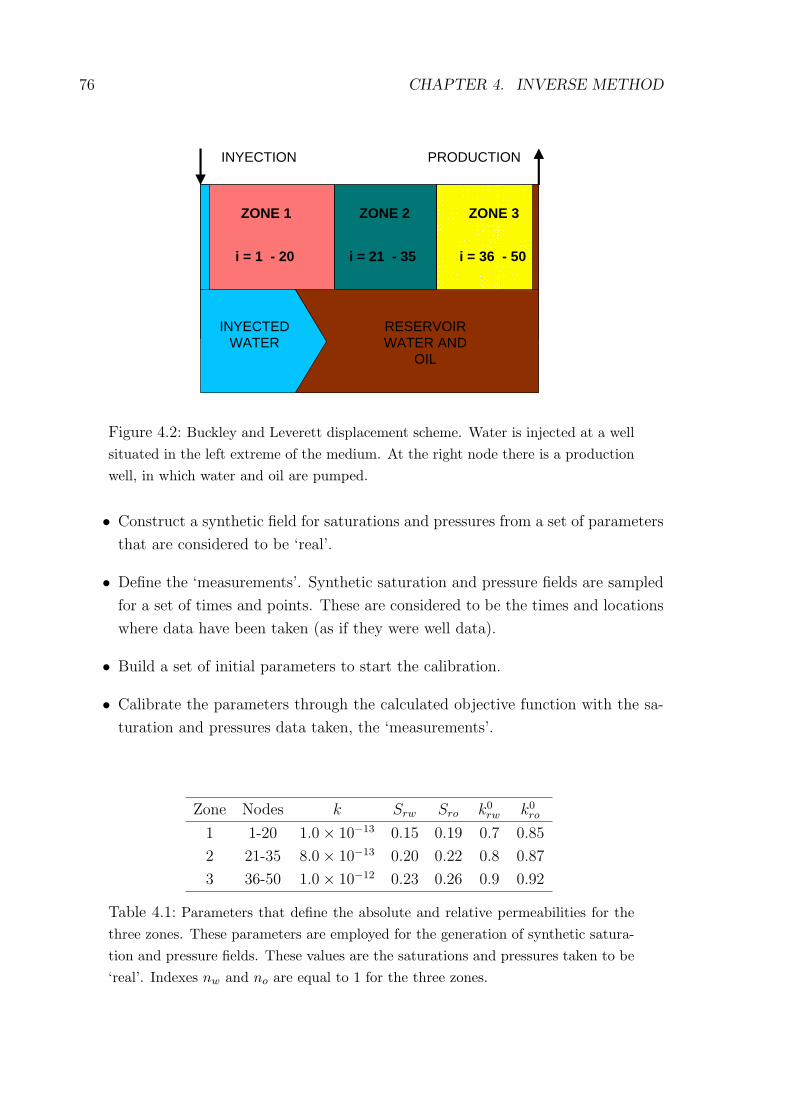
76 CHAPTER 4. INVERSE METHOD
ZONE 1 ZONE 2 ZONE 3
i = 1 - 20 i = 21 - 35 i = 36 - 50
INYECTION PRODUCTION
INYECTEDWATER
RESERVOIRWATER AND
OIL
Figure 4.2: Buckley and Leverett displacement scheme. Water is injected at a wellsituated in the left extreme of the medium. At the right node there is a productionwell, in which water and oil are pumped.
• Construct a synthetic field for saturations and pressures from a set of parameters
that are considered to be ‘real’.
• Define the ‘measurements’. Synthetic saturation and pressure fields are sampled
for a set of times and points. These are considered to be the times and locations
where data have been taken (as if they were well data).
• Build a set of initial parameters to start the calibration.
• Calibrate the parameters through the calculated objective function with the sa-
turation and pressures data taken, the ‘measurements’.
Zone Nodes k Srw Sro k0rw k0
ro
1 1-20 1.0× 10⁻¹³ 0.15 0.19 0.7 0.85
2 21-35 8.0× 10⁻¹³ 0.20 0.22 0.8 0.87
3 36-50 1.0× 10⁻¹² 0.23 0.26 0.9 0.92
Table 4.1: Parameters that define the absolute and relative permeabilities for thethree zones. These parameters are employed for the generation of synthetic satura-tion and pressure fields. These values are the saturations and pressures taken to be‘real’. Indexes nw and no are equal to 1 for the three zones.

4.4. APPLYING THE INVERSE METHOD 77
0.1
0.2
0.3
0.4
0.5
0.6
0.7
0.8
0.9
1.0
0 100 200 300 400 500x (m)
Sw
Kabs. = real & Krel. = real Kabs. = initial & Krel. = initialKabs. = real & Krel. = initial
Figure 4.3: Saturation front corresponding to the numerical solution at the end of the si-mulation. The blue curve represents the real case, the pink curve the initial results, and thegreen curve the saturation front when using the real values for absolute permeability and theinitial parameters for relative permeability curves.
The study area is discretized with a regular grid of 50 grid blocks. The medium
has been divided in three zones, within each of them permeability is considered to be
homogeneous. Grid blocks corresponding to each of the zones are graphed in figure
4.2. Parameters that describe the reality, which normally is not known, are resumed
in Table 4.1. In this example heterogeneity for both absolute and relative permeability
is built per zones. 500 time steps are used. The analysis is carried out assuming that
there are three data points at grid blocks i = 10, 25, 40, one per zone, for 10 times
(t = 50, 100, 150, 200, 250, 300, 350, 400, 450 and 500). These measurements are
directly read from the synthetic results.
k Srw Sro k0rw k0
ro
5.0× 10⁻¹³ 0.10 0.15 0.68 0.70
Table 4.2: Initial parameters taken for the example calibration. These parametersdefine relative permeability curves and absolute permeability in the three zones inwhich the domain is divided. Indexes nw and no are equal to 1 for the three zones.

78 CHAPTER 4. INVERSE METHOD
6.0E+06
6.2E+06
6.4E+06
6.6E+06
6.8E+06
7.0E+06
7.2E+06
7.4E+06
7.6E+06
7.8E+06
8.0E+06
0 100 200 300 400 500x (m)
Pre
ssur
e (P
a)
Kabs. = real & Krel. = real Kabs. = intial & Krel. = initialKabs. = real & Krel. = initial
Figure 4.4: Pressure front corresponding to the numerical solution at the end ofthe simulation. The blue curve represents the real case, the pink curve the initialresults, and the green curve the saturation front when using the real values forabsolute permeability and the initial parameters for relative permeability curves.
For the calibration it is necessary to start from a set of initial values, summarized
in Table 4.2. These parameters have been defined as homogeneous for all the domain.
In the Figures 4.3 and 4.4 saturation and pressure are graphed for all the nodes at the
last time step simulated. Blue curve represents the output values given by the two-
phase numerical flow solver with real parameter values in Table 4.1. The pink curve
corresponds to the numerical solution using initial parameter values in Table 4.2.
The objective of this exercise is to check the importance of calibrating or not cali-
brating relative permeability curves. The results are going to corroborate results shown
in chapter 2, the saturation front is much more influenced by the relative permeability
curves than the pressure front. Indeed, no calibration is necessary to arrive to that
conclusion. If saturation and pressure fronts are computed with the forward two-phase
flow simulator, assuming that absolute permeability is known, but relative permeability
values are unknown and assigned to be equal to the initial values (Table 4.2), the result
is very interesting. Saturation and pressure fronts are graphed in Figures 4.3 and 4.4
with the green curves. It can be seen that the pressure field does not change so much
with respect the real values given by the blue curve, while the saturation front is highly
affected. This property of relative permeabilities can be taken into account when the
optimization algorithm is programmed. If the pressure term in the objective function

4.4. APPLYING THE INVERSE METHOD 79
0.1
0.2
0.3
0.4
0.5
0.6
0.7
0.8
0.9
1.0
0 100 200 300 400 500x (m)
Sw
Kabs. = real & Krel. = realKabs. = initial & Krel. = initialKabs. = calibrated & Krel. = calibrated
Figure 4.5: Saturation front corresponding to the calibrated parameters. Results for thelast simulation time. The blue curve corresponds to real values, the pink one to the initial.The green curve is the result after the simultaneous calibration of relative and absolutepermeabilities.
has been reduced considerably, but not for the saturation term, weight for pressures
wp can be assigned to be zero and optimization can continue only for parameters of
relative permeability curves.
When the calibration is run the starting parameter values, given in Table 4.2, are
modified iteratively to end up with the values given in Table 4.3. The saturation and
pressure fronts given by the calibrated parameters are represented by the green curves
in Figures 4.5 and 4.6. In the calibration presented here it was employed a weight
for the pressures (wp,i in equation (4.1)) equal to 10−10, obtaining with it an initial
objective function value of 149.98. Saturation weights for all the examples taken in
this dissertation are equal to 1. This means that saturation measurements are assumed
to be free of any error. Saturation errors can be taken into account by just changing
this value. The election of the pressure weight wp in the objective function was made
after several tries with different weights. The value chosen was the one that resulted
in an objective function with an order of magnitude low enough to perform the inverse
modeling. After 323 iterations the objective function resulted equal to 0.00176. The
match was considered very optimum for both saturation and pressure fields (see Figures
4.5 and 4.6).

80 CHAPTER 4. INVERSE METHOD
6.0E+06
6.2E+06
6.4E+06
6.6E+06
6.8E+06
7.0E+06
7.2E+06
7.4E+06
7.6E+06
7.8E+06
8.0E+06
0 100 200 300 400 500x (m)
Pre
ssur
e (P
a)
Kabs. = real & Krel. = realKabs. = initial & Krel. = initialKabs. = calibrated & Krel. = calibrated
Figure 4.6: Pressure front corresponding to the calibrated parameters. Results forthe last simulation time. The blue curve corresponds to real values, the pink oneto the initial. The green curve is the result after the simultaneous calibration ofrelative and absolute permeabilities.
For this exercise the evolution of the objective function for the first 100 iterations
has been graphed in Figure 4.7. The y axis corresponds to the objective function and
it has been plotted in logarithm scale. For the first 5 iterations, when the objective
function is bigger than 2, the weight value of the saturations has been set to zero,
ws = 0. This has been done because until that point the contribution for the objective
function is mainly due to the pressure term. This avoids to compute the gradient for
the relative permeability parameters for the first iterations.
Zone Nodes k Srw Sro k0rw k0
ro
1 1-20 1.0× 10⁻¹³ 0.145 0.194 0.608 0.738
2 21-35 8.0× 10⁻¹³ 0.203 0.215 0.890 0.867
3 36-50 1.0× 10⁻¹² 0.211 0.230 0.759 0.827
Table 4.3: Parameter values obtained after the simultaneous calibration of relativeand absolute permeability fields in the three zones.

4.4. APPLYING THE INVERSE METHOD 81
1.E-03
1.E-02
1.E-01
1.E+00
1.E+01
1.E+02
1.E+03
0 20 40 60 80 100
Number of iterations
Log
(Obj
ectiv
e Fu
nctio
n)
Figure 4.7: The objective function (in logarithm scale) is represented in function ofthe number of iterations for 1D example.
This simple example shows that the inverse method developed works and it is
capable to match the production data. The technique is ready to be applied to more
complex 1D and 2D cases, and to perform uncertainty analysis. Next chapters present
these applications.

82 CHAPTER 4. INVERSE METHOD

Chapter 5
Calibrating absolute and relative
permeabilities in 2D
The main objective of this dissertation is to produce a technique that simultaneously
calibrate (or inverse model) both absolute and relative permabilities, considering both
parameters spatially variable within the reservoir. Former chapters have extensively
described the most important basic concepts of the inverse method developed. The
present chapter shows several applications of this method in one and two dimensions
for different reservoir configurations. In first place, calibrations of absolute and relative
permeability fields in two dimensions are shown. Also one calibration with seismic data
as dynamic variable plus production data is analyzed.
In the following examples absolute permeability heterogeneity is closer to a real re-
servoir representation than the heterogeneities used for 1D cases. These heterogeneities
are similar to the field presented in chapter 3 (Figure 3.14). Relative permeabilities are
still assumed to be homogeneous within different areas in which the domain is divided
in all the analyzed cases, except in one example. To make the hypothetical problem
closer to a real case, extra data are supposed to be available, like absolute permeability
measurements or seismic information. This additional information has a major impor-
tance for a good agreement between reality and calibrated results. First, three test
problems were run: quarter five spot configuration with production data, quarter five
spot configuration with production and seismic data and vertical section with produc-
tion data. A final forth example was carried out with relative permeabilities varying
all over the domain.
Discretization and size taken in the cases performed in this dissertation are chosen
to make the problems easy to compute. It is the aim of this research to develope a
new inverse technique, to test the possibilities to run it, and to see how this technique
can improve reservoir characterization. Future research must look for optimization
83

84 CHAPTER 5. CALIBRATING K AND KREL IN 2D
techniques to speed up the forward and inverse simulator in order to perform more
realistic cases with higher discretizations and domain size.
5.1 Relative permeability field given in zones: quar-
ter five spot case.
INJECTOR
PRODUCTOR
k°_rw =0.7 k°_ro =0.75
S_rw =0.1 S_ro =0.18
k°_rw =0.8 k°_ro =0.85
S_rw =0.2 S_ro =0.23
k°_rw =0.87 k°_ro =0.90
S_rw =0.26 S_ro =0.29ZONE 3
ZONE 2
ZONE 1
Figure 5.1: The quarter five spot scheme is represented in this figure, injector situa-ted at lower left corner, and producer at upper right corner. The reservoir is dividedinto 3 different zones, within each of them the relative permeability parameters areassumed to be constant. The true values for the relative permeability parametersare also resumed in the figure.
The first example chosen for a 2D immiscible two-phase flow was the so called
quarter five spot problem, which is a model problem in reservoir engineering. The
spatial domain is a horizontal cut of an oil field, where a periodic arrangement of
injection and production wells is considered. Figure 5.1 should clear the setting. In
one space dimension this problem simplifies to Buckley-Leverett displacement problem,
used in former chapters.
As in 1D, a synthetic case is created. 15 by 15 grid blocks are used to discretized
the 2D domain with no flow boundaries. Reservoir performance was simulated using
a uniform spatial grid with ∆x = ∆y = 10m. Remember that the objective of the

5.1. QUARTER FIVE SPOT CASE 85
log KABSOLUTE
East
Nor
th
0.0 150.000.0
150.00
-13.500
-13.000
-12.500
-12.000
-11.500
Figure 5.2: 2D heterogeneous absolute permeability field that is taken as the real absolutepermeability field.
SATURATIONS
East
Nor
th
0.0 150.000.0
150.00
0.0
0.1000
0.2000
0.3000
0.4000
0.5000
0.6000
0.7000
0.8000
0.900
1.000
(a) Sw
PRESSURES
East
Nor
th
0.0 150.000.0
150.00
4500000.
5000000.
5500000.
6000000.
6500000.
7000000.
7500000.
8000000.
8500000.
9000000.
9500000.
(b) P
Figure 5.3: When introducing real parameters in the two-phase flow simulator this is thesaturation (a) and pressure (b) field obtained at the end of the simulation.
exercise is just to check the feasibility of the inverse technique, this is the reason why
the discretization is so simple. Absolute permeability is heterogeneous all over the
reservoir, but relative permeability is constant within some areas (schemed in Figure
5.1). No statistical correlation was considered between the five parameters (k, k0rw,
Srw, k0ro and Sro). However, there is an implicit correlation as all the parameters are
calibrated to the same set of production data. Three relative permeability curves (one
per zone) are considered to describe the domain. Parameters corresponding to these
water and oil relative permeability curves are resumed in Figure 5.1. The sequential
Gaussian simulation code GCOSIM3D (Gomez-Hernandez and Journel, 1993) was run
in order to generate heterogenous absolute permeability field. The resulting real lo-
garithm absolute permeability field is shown in Figure 5.2. The absolute permeability

86 CHAPTER 5. CALIBRATING K AND KREL IN 2D
(a) Configuration 1 (b) Configuration 2
Figure 5.4: Master point positions for inversion modeling. Red circles correspondto absolute permeability master points and yellow starts to relative permeabilitymaster points.
distribution is assumed to be log-normal with log-mean equal to -13.0 and variance
equal to 0.3. It is also assumed that absolute permeability field is isotropic and spatial
continuity can be described with a spherical variogram model of range equal to 60 m.
Another relevant reservoir property is the porosity, being φ = 0.2. The parameter set
given by Figures 5.1 and 5.2 are assigned to be the real values for this example and
the next two sections.
Initially, the saturation conditions are considered homogeneous. The reservoir is
almost full with oil (90%), and the rest (10%) is filled with water. Water is injected
through a well situated in the lower left corner of the computational domain (Figure
Figure 5.5: Grid blocks positions at which absolute permeability and productiondata are available. They are indicated with orange squares.

5.1. QUARTER FIVE SPOT CASE 87
log KABSOLUTE
East
Nor
th
0.0 150.000.0
150.00
-13.500
-13.000
-12.500
-12.000
-11.500
(a) Initial logk
log KABSOLUTE
East
Nor
th
0.0 150.000.0
150.00
-13.500
-13.000
-12.500
-12.000
-11.500
(b) Calibrated logk
log KABSOLUTE
East
Nor
th
0.0 150.000.0
150.00
-13.500
-13.000
-12.500
-12.000
-11.500
(c) Real logk
SATURATIONS
East
Nor
th
0.0 150.000.0
150.00
0.0
0.1000
0.2000
0.3000
0.4000
0.5000
0.6000
0.7000
0.8000
0.900
1.000
(d) Initial Sw
SATURATIONS
East
Nor
th
0.0 150.000.0
150.00
0.0
0.1000
0.2000
0.3000
0.4000
0.5000
0.6000
0.7000
0.8000
0.900
1.000
(e) Calibrated Sw
SATURATIONS
East
Nor
th
0.0 150.000.0
150.00
0.0
0.1000
0.2000
0.3000
0.4000
0.5000
0.6000
0.7000
0.8000
0.900
1.000
(f) Real Sw
PRESSURES
East
Nor
th
0.0 150.000.0
150.00
4500000.
5000000.
5500000.
6000000.
6500000.
7000000.
7500000.
8000000.
8500000.
9000000.
9500000.
(g) Initial P
PRESSURES
East
Nor
th
0.0 150.000.0
150.00
4500000.
5000000.
5500000.
6000000.
6500000.
7000000.
7500000.
8000000.
8500000.
9000000.
9500000.
(h) Calibrated P
PRESSURES
East
Nor
th
0.0 150.000.0
150.00
4500000.
5000000.
5500000.
6000000.
6500000.
7000000.
7500000.
8000000.
8500000.
9000000.
9500000.
(i) Real P
Figure 5.6: In this figure initial (first column), calibrated (second column) and real (thirdcolumn) realizations are presented for comparison. First row corresponds to logarithm ofabsolute permeability, second row to water saturations after 120 days and third column topressures after 120 days. Well layout has the form of a quarter five spot problem. Inversionwith 5 production data points and 4 absolute permeability measurements was run.
5.1). Water and oil are produced through a well in the upper right corner (Figure 5.1).
The absolute and relative permeability realizations, considered as real representations
of the reservoir, are introduced in the forward two-phase solver. The initial conditions
are Sw = 0.1 and P = 6.895× 10⁶ Pa. Water is injected into the porous medium filled

88 CHAPTER 5. CALIBRATING K AND KREL IN 2D
with oil and water at constant rate of 2.5kg/s. Production rate is also constant and
equal to 2.5kg/s. For the following examples mobility ratio is taken to be equal to
one, k0rwµo/k
0roµw = 1, and exponents nw = no = 1. Constant 4.8 hours time steps are
prescribed, an the simulation is run to 120 days. Saturation and pressure fields after
the 120 days are given in Figures 5.3(a) and 5.3(b). They represent the behavior of
the reservoir assumed to be real.
The hypothetical data production measurements are located in 5 selected grid
blocks, indicated in Figure 5.5 with orange squares. Data values are supposed to
be measured for 10 times of the 600 time steps during which the forward simulator was
run. These are the data introduced in the objective function, SMEASw and pMEAS, and
the values that are going to be reproducted with the inversion.
Iterations start from an initial set of absolute and relative permeabilities. Initial
absolute field is given in Figure 5.6(a). The initial relative permeability field is taken
to be homogeneous all over the domain. The parameters that define this relative
permeability curve are resumed in Tables 5.1 and 5.2. For the last time step of the
simulation the saturation and pressure fields with these initial parameters are shown
in Figures 5.6(d) and 5.6(g), respectively.
In the inversion, the parameter space is reduced by the definition of a set of points
for the perturbation, called master points. For the calibration the number and lo-
cations of the master points must be selected. Capilla et al. (1997) found that 3
master blocks per correlation range was optimal. Here, 3 master points are taken for
relative permeabilities (yellow starts in Figure 5.4) and 11 master points for absolute
permeability (red circles in Figure 5.4). Hendricks-Franssen (2001) suggests that if the
master blocks configuration changes as the iterations proceed the procedure yields a
faster convergence. Two different master point configurations where selected in this
test problem, which are shown in Figures 5.4(a) and 5.4(b). During the calibration
the configuration of master blocks switches between both of them. In 5 grid blocks
(orange squares in Figure 5.6) absolute permeability measurements are supposed to be
available. The 5 corresponding master points will have a perturbation equal to zero
during all the calibration.
With this configuration, the total parameter space to be calibrated is: (5 parame-
ters k, k0rw, Srw, k0
ro, Sro) x (11 + 3 master points - 5 k data points). This means that
the forward simulator must be run in each iteration 45 times, for the computation of
the gradient components, plus the runs required in the linear optimization for the cal-
culation of α (perturbation size, equation (4.2)). In order to slow down the simulation
time in each iteration it has been decided to avoid the linear optimization. Instead,
the size of the perturbation is fixed, and gradually decreased while the objective func-

5.1. QUARTER FIVE SPOT CASE 89
Zone k0rw k0
ro
Initial Calibrated Real Initial Calibrated Real
1 0.911 0.991 0.700 0.911 0.896 0.750
2 0.911 0.924 0.800 0.911 0.954 0.850
3 0.911 0.988 0.870 0.911 0.978 0.900
Table 5.1: Initial, calibrated and real values for water and oil end-points of relativepermeability curves. The calibration test case is a quarter five spot problem with 5production data points in 10 times and 5 absolute permeability measurements.
tion diminishes. This is a compromise solution that results in a quite high number
of iterations necessary to arrive to the minimum objective function. For this example
the calibration process was stopped after 3000 iterations, when the objective function
seemed to be low enough.
Zone Srw Sro
Initial Calibrated Real Initial Calibrated Real
1 0.245 0.034 0.100 0.245 0.196 0.180
2 0.245 0.270 0.200 0.245 0.272 0.230
3 0.245 0.165 0.260 0.245 0.433 0.290
Table 5.2: Initial, calibrated and real values for water and oil residual saturations.The calibration test case is a quarter five spot problem with 5 production datapoints in 10 times and 5 absolute permeability measurements.
In general the output given by the calibration reveals that the inverse technique can
perform the calibration in two dimensions. Some of the results after the calibration are
resumed in Figure 5.6. Absolute permeability fields are represented in Figures 5.6(a)
to 5.6(c) (for initial, calibrated and real cases), and saturation and pressure responses
after 120 days, shown in Figures 5.6(d) to 5.6(f) and Figures 5.6(g) to 5.6(i), also for
initial, calibrated and real cases. A preliminary qualitative evaluation of the calibration
method follows.
Calibrated absolute permeability (Figure 5.6(b)) smooths some of the high and low
initial values (Figure 5.6(a)) which do not match with the true field (Figure 5.6(c)).
Anyway, the areas where no production data is located, neither absolute permeabilities
are available, are not well calibrated. Look for example, the high values (red spot)

90 CHAPTER 5. CALIBRATING K AND KREL IN 2DS
imul
ated
Sw
Observed Sw
Observed - Simulated Sw at data wells
0.00 0.20 0.40 0.60 0.80 1.00
0.00
0.20
0.40
0.60
0.80
1.00Number of data 50Number plotted 50
X Variable: mean 0.44std. dev. 0.32
Y Variable: mean 0.45std. dev. 0.33
correlation 0.90rank correlation 0.93
(a) Before inversionS
imul
atea
d S
w
Observed Sw
Observed - Simulated Sw at data wells
0.00 0.20 0.40 0.60 0.80 1.00
0.00
0.20
0.40
0.60
0.80
1.00Number of data 50Number plotted 50
X Variable: mean 0.44std. dev. 0.32
Y Variable: mean 0.41std. dev. 0.31
correlation 0.99rank correlation 0.98
(b) After inversion
Obs
erve
d P
x 1
e6
Simulated P x 1e6
Observed - Simulated P at data wells
3.0 7.0 11.0 15.0
3.0
7.0
11.0
15.0
Number of data 50Number plotted 50
X Variable: mean 6.97std. dev. 1.37
Y Variable: mean 7.95std. dev. 4.54
correlation 0.85rank correlation 0.97
(c) Before inversion
Sim
ulat
ed P
x 1
e6
Observed P x 1e6
Observed - Simulated P at data wells
3.0 7.0 11.0 15.0
3.0
7.0
11.0
15.0
Number of data 50Number plotted 50
X Variable: mean 6.97std. dev. 1.37
Y Variable: mean 6.87std. dev. 1.39
correlation 0.99rank correlation 0.98
(d) After inversion
Figure 5.7: Simulated versus observed values are plotted for the results before and afterthe inversion is performed. The graphs presented here correspond to the quarter five spotconfiguration with 5 data wells and 10 times of measurements. Figures (a) and (b) are thescatter plots for water saturations and (c) and (d) for pressures.
situated in middle left zone. However, the pressure front (Figure 5.6(h)) matches quite
well the true values (Figure 5.6(i)). The same happens with the saturation field, in
which the different values related with the relative permeability curves are reflected
after the calibration (Figure 5.6(e)). Initial values for relative permeability curves
where taken to be homogenous (Tables 5.1 and 5.2) and this is reflected in the shape
of the initial saturation front (Figure 5.6(d)). After calibration, though the relative
permeability parameter values are not matched, with them a better reproduction of the
saturation front is achieved (compare Figures 5.6(e) and 5.6(f)). It can be said that the

5.1. QUARTER FIVE SPOT CASE 91
inversion is well performed and the saturation and pressure data are well reproduced.
When no data are available it is normal to find some disagreements between real and
simulatead fields. This is what it is reflected in the results found in this test case. The
inverse method works and can perform an inversion as the data values are matched.
The calibrated permeability fields shown in Figure 5.6(c) and Tables 5.1 and 5.2
are one possible representation of the reservoir. Indeed, if other input parameters
are considered for the initial values the calibrated permeabilities would be different.
These examples are shown in order to check that the inverse technique works, however
the method must be complemented with an uncertainty study, which is going to be
presented in next chapter.
For a quantitative evaluation of the results two different kind of plots have been
performed. First, scatter plots for saturation and pressure at well data are graphed.
Figure 5.7 compares the production data misfit before (Figures 5.7(a) and (c)) and
after the calibration (Figures 5.7(b) and (d)). Though the results still do not match
exactly the observed saturation and pressures, the calibration reduces the spread of
the scatter plot.
Because this is a synthetic case, true values for saturation and pressure are available
all over the domain for every time step. Another way to measure the misfit between
the true and simulated values is with the definition of the residuals R:
Rts,i = (SSIM
i,t − SMEASi,t )
Rtp,i = (pSIM
i,t − pMEASi,t )
(5.1)
for saturations, Rs, and pressures, Rp, at grid block i and time step t. The histograms
of the residuals for 6 time steps are plotted in Figures 5.8 and 5.9. All the histograms
are fairly symmetric and do not have long tails. Saturation residuals for first time
steps reflect a tendency towards underestimation (negative mean), while overestimation
appears for last times. Saturation estimations are quite unbiased as both mean and
median error are close to zero. In general pressure values seem to be underestimated.
Mean values are very close to zero while the median expresses some asymmetry in
the errors. Saturation and pressure error distributions present a small spread. These
results show that for the data grid blocks the observed values are well reproduced
(Figure 5.7), while when looking at the whole field some disagreements must exist and
consecuently the histograms indicate residuals different from zero.

92 CHAPTER 5. CALIBRATING K AND KREL IN 2D
Fre
quen
cy
-1.00 -0.50 0.00 0.50 1.00
0.000
0.100
0.200
0.300
0.400
0.500
0.600
0.700Residual Sw t=100
Number of Data 225
mean -0.0002std. dev. 0.0478
coef. of var undefined
maximum 0.1706upper quartile 0.0005
median 0.0001lower quartile -0.0002
minimum -0.1870
(a) t=100
Fre
quen
cy
-1.00 -0.50 0.00 0.50 1.00
0.000
0.100
0.200
0.300
0.400
0.500
0.600
0.700Residual Sw t=200
Number of Data 225
mean -0.0005std. dev. 0.0969
coef. of var undefined
maximum 0.3595upper quartile 0.0185
median 0.0002lower quartile -0.0001
minimum -0.3905
(b) t=200
Fre
quen
cy
-1.00 -0.50 0.00 0.50 1.00
0.000
0.100
0.200
0.300
0.400
0.500
0.600
0.700Residual Sw t=300
Number of Data 225
mean -0.0006std. dev. 0.1378
coef. of var undefined
maximum 0.5201upper quartile 0.0286
median 0.0005lower quartile -0.0124
minimum -0.4825
(c) t=300
Fre
quen
cy
-250. -150. -50. 50. 150. 250.
0.000
0.100
0.200
0.300Residual P (psi) t=400
Number of Data 225
mean -0.5706std. dev. 48.2812
coef. of var undefined
maximum 93.7200upper quartile 41.4900
median -0.5272lower quartile -39.4425
minimum -142.0000
(d) t=400
Fre
quen
cy
-1.00 -0.50 0.00 0.50 1.00
0.000
0.100
0.200
0.300
0.400
0.500
0.600
0.700Residual Sw t=500
Number of Data 225
mean 0.0145std. dev. 0.1440
coef. of var undefined
maximum 0.4257upper quartile 0.0754
median 0.0186lower quartile -0.0210
minimum -0.4476
(e) t=500
Fre
quen
cy
-1.00 -0.50 0.00 0.50 1.00
0.000
0.100
0.200
0.300
0.400
0.500
0.600
0.700Residual Sw t=600
Number of Data 225
mean 0.0178std. dev. 0.1424
coef. of var undefined
maximum 0.4075upper quartile 0.0836
median 0.0309lower quartile -0.0009
minimum -0.4407
(f) t=600
Figure 5.8: Histograms for the saturation residuals defined in equation (5.1). 6 time stepsare chosen: t = 100, t = 200, t = 300, t = 400, t = 500 and t = 600 (graphs (a) to (f)). Thegraphs presented here correspond to the quarter five spot configuration with 5 productiondata grid blocks, absolute permeability data in 5 grid blocks, and production data availablefor 10 times.

5.1. QUARTER FIVE SPOT CASE 93
Fre
quen
cy
-250. -150. -50. 50. 150. 250.
0.000
0.100
0.200
0.300Residual P (psi) t=100
Number of Data 225
mean -0.2711std. dev. 39.3565
coef. of var undefined
maximum 79.6200upper quartile 30.7275
median 3.2110lower quartile -33.1850
minimum -120.4000
(a) t=100
Fre
quen
cy
-250. -150. -50. 50. 150. 250.
0.000
0.100
0.200
0.300Residual P (psi) t=200
Number of Data 225
mean -0.4799std. dev. 42.4193
coef. of var undefined
maximum 86.6400upper quartile 34.7525
median 2.3280lower quartile -36.2975
minimum -124.7000
(b) t=200
Fre
quen
cy
-250. -150. -50. 50. 150. 250.
0.000
0.100
0.200
0.300Residual P (psi) t=300
Number of Data 225
mean -0.5792std. dev. 45.7595
coef. of var undefined
maximum 91.0500upper quartile 39.1475
median 0.8411lower quartile -39.7050
minimum -131.2000
(c) t=300
Fre
quen
cy
-600. -200. 200. 600.
0.000
0.100
0.200
0.300
0.400
0.500
0.600Residual P (psi) t=400
Number of Data 225
mean -0.4063std. dev. 45.0710
coef. of var undefined
maximum 85.2300upper quartile 35.9000
median 3.9890lower quartile -39.3450
minimum -131.5000
(d) t=400
Fre
quen
cy
-250. -150. -50. 50. 150. 250.
0.000
0.100
0.200
0.300Residual P (psi) t=500
Number of Data 225
mean -1.0731std. dev. 49.9833
coef. of var undefined
maximum 94.8300upper quartile 42.4175
median -1.3140lower quartile -39.9350
minimum -151.8000
(e) t=500
Fre
quen
cy
-250. -150. -50. 50. 150. 250.
0.000
0.100
0.200
0.300Residual P (psi) t=600
Number of Data 225
mean -1.1222std. dev. 50.4734
coef. of var undefined
maximum 95.3000upper quartile 42.7475
median -1.5250lower quartile -40.4100
minimum -153.7000
(f) t=600
Figure 5.9: Histograms for the pressure residuals defined in equation (5.1). 6 time steps arechosen: t = 100, t = 200, t = 300, t = 400, t = 500 and t = 600 (graphs (a) to (f)). Thegraphs presented here correspond to the quarter five spot configuration with 5 productiondata grid blocks, absolute permeability data in 5 grid blocks, and production data availablefor 10 times.

94 CHAPTER 5. CALIBRATING K AND KREL IN 2D
5.2 Relative permeability field given in zones: seis-
mic data case
Important decisions in the petroleum industry are based on information from seismic
data. Seismic data are originated from acoustic pulses generated on the earth’s surface.
They are the record of the reflection from the earth’s interior. During the last years the
geophysics field has developed and refined the 3D and 4D seismic technology. The 3D
seismic data comes from a high resolution seismic survey that allows a more detailed
three dimensional characterization of the subsurface. When two or more successive 3D
surveys are shot over the same area the process is referred to as 4D seismic, to denote
the addition of the time dimension.
SATURATIONS
East
Nor
th
0.0 150.000.0
150.00
0.0
0.1000
0.2000
0.3000
0.4000
0.5000
0.6000
0.7000
0.8000
0.900
1.000
Figure 5.10: Simulated seismic data corresponding to the real water saturationfield. The procedure followed was to add a random noise to the water saturationfield given in 5.3(a), which corresponds to the last simulation time step. The sameprocedure has been applied to 10 different time steps.
In general, seismic images are sensitive to the spatial variation of two distinct types
of reservoir properties: static geologic properties, as lithology, porosity, cementation or
shale content, and dynamic fluid flow properties as saturation and pore pressures. By
comparing the data from 3D surveys acquired at different times at the same location,
it is possible to eliminate the effects of unknown static properties to focus on the
dynamic changes in production related properties. So, the sensitivity to saturation
changes allows tracking of the movement of fronts in the reservoir. The outstanding
characteristic of the 4D seismic data is that it provides areally distributed information,
which can therefore provide a higher areal resolution than well data. With this process,
it is possible to estimate the areal distribution of saturation changes in the reservoir
due to the production or injection of fluids.
For inverse modeling in reservoir simulation, it is possible to take advantage of this

5.2. SEISMIC DATA CASE 95
log KABSOLUTE
East
Nor
th
0.0 150.000.0
150.00
-13.500
-13.000
-12.500
-12.000
-11.500
(a) Initial logk
log KABSOLUTE
East
Nor
th
0.0 150.000.0
150.00
-13.500
-13.000
-12.500
-12.000
-11.500
(b) Calibrated logk
log KABSOLUTE
East
Nor
th
0.0 150.000.0
150.00
-13.500
-13.000
-12.500
-12.000
-11.500
(c) Real logk
SATURATIONS
East
Nor
th
0.0 150.000.0
150.00
0.0
0.1000
0.2000
0.3000
0.4000
0.5000
0.6000
0.7000
0.8000
0.900
1.000
(d) Initial Sw
SATURATIONS
East
Nor
th
0.0 150.000.0
150.00
0.0
0.1000
0.2000
0.3000
0.4000
0.5000
0.6000
0.7000
0.8000
0.900
1.000
(e) Calibrated Sw
SATURATIONS
East
Nor
th
0.0 150.000.0
150.00
0.0
0.1000
0.2000
0.3000
0.4000
0.5000
0.6000
0.7000
0.8000
0.900
1.000
(f) Real Sw
PRESSURES
East
Nor
th
0.0 150.000.0
150.00
4500000.
5000000.
5500000.
6000000.
6500000.
7000000.
7500000.
8000000.
8500000.
9000000.
9500000.
(g) Initial P
PRESSURES
East
Nor
th
0.0 150.000.0
150.00
4500000.
5000000.
5500000.
6000000.
6500000.
7000000.
7500000.
8000000.
8500000.
9000000.
9500000.
(h) Calibrated P
PRESSURES
East
Nor
th
0.0 150.000.0
150.00
4500000.
5000000.
5500000.
6000000.
6500000.
7000000.
7500000.
8000000.
8500000.
9000000.
9500000.
(i) Real P
Figure 5.11: In this figure initial (first column), calibrated (second column) and real (thirdcolumn) realizations are presented for comparison. First row corresponds to logarithm ofabsolute permeability, second row to water saturations after 120 days and third column topressures after 120 days. Well layout has the form of a quarter five spot problem. Inversionwith 3 absolute permeability data, 3 pressure well data and seismic information was run.
properties of 4D seismic to improve the resolution of the calibrations. This has been
carried out by Landa (1997), Idrobo et al. (1999) or Wen et al. (2002). Following the
same process, here it is presented a synthetic case in which 4D seismic are supposed
to be available. The inversion is performed by using 4D seismic data and absolute

96 CHAPTER 5. CALIBRATING K AND KREL IN 2D
permeability data. Let’s see how the inversion technique performs.
Zone k0rw k0
ro
Initial Calibrated Real Initial Calibrated Real
1 0.629 0.764 0.700 0.629 0.740 0.750
2 0.629 0.499 0.800 0.629 0.741 0.850
3 0.629 0.519 0.870 0.629 0.641 0.900
Table 5.3: Initial, calibrated and real values for water and oil end-points of relativepermeability curves. Calibration was performed for a quarter five spot problem withseismic data, 3 absolute permeability grid block data nd 3 pressure well measure-ments.
The true permeability fields are the ones taken in the former section (Figures 5.1
and 5.2), with relative permeabilities taken to be homogeneous within 3 different areas
in which the domain can be divided and absolute permeability heterogenous all over
the domain. The quarter five spot configuration described before is considered. The
same initial conditions (Sw = 0.1, P = 6.895 × 10⁶ Pa) and other parameters like
φ = 0.2, production/injection rate = 2.5kg/s, unit mobility ratio and nw = no = 1.
Instead of having saturation production data, seismic data are assumed to be available.
True water saturation and pressure fields after the 120 days of production are given in
Figures 5.3(a) and 5.3(b). To simulate seismic data water saturation plus a percentage
random noise is taken. Let’s suppose that seismic campaign has been done for 10
times. 10 simulated seismic field images are obtained by adding random noise to
the water saturation realizations corresponding to these 10 times. The seismic image
corresponding to water saturation in Figure 5.3(a) (t = 120 days) is drawn in Figure
5.10.
The objective function can take into account the error that water saturations have
when they are deduced from seismic 4D data. Pressure data are assign to be taken
at 3 grid blocks (injector, productor and an additional situated in the central grid
block) for the same 10 times that seismic data are available. In these 3 wells absolute
permeability measurements are availabe (instead of the 5 assumed in the former test
problem). After 2014 iterations the calibration is good enough. In the inversion process
3 master points were taken for the relative permeabilities (one per zone), while for the
absolute permeability 11 master points were selected, 3 of them corresponding to the
absolute permeability measurements (hence, no perturbation is applied to this 3 master
points). Absolute permeability master point positions are plotted with red circles in
Figure 5.4(a). Yellow starts in Figure 5.4(a) represent relative permeability master

5.2. SEISMIC DATA CASE 97
Zone Srw Sro
Initial Calibrated Real Initial Calibrated Real
1 0.105 0.112 0.100 0.105 0.177 0.180
2 0.105 0.170 0.200 0.105 0.235 0.230
3 0.105 0.152 0.260 0.105 0.264 0.290
Table 5.4: Initial, calibrated and real values for water and oil residual saturations.Calibration was performed for a quarter five spot problem seismic data, 3 absolutepermeability grid block data nd 3 pressure well measurements.
points. As in the former section, initial, calibrated and real fields are going to be
qualitatively analyzed.
Obs
erve
d P
x 1
e6
Simulated P x 1e6
Observed - Simulated P at data wells
3.0 7.0 11.0 15.0
3.0
7.0
11.0
15.0
Number of data 50Number plotted 50
X Variable: mean 6.97std. dev. 1.37
Y Variable: mean 7.95std. dev. 4.54
correlation 0.85rank correlation 0.97
(a) Before inversion
Sim
ulat
ed P
x 1
e6
Observed P x 1e6
Observed - Simulated P at data wells
3.0 7.0 11.0 15.0
3.0
7.0
11.0
15.0
Number of data 50Number plotted 50
X Variable: mean 6.97std. dev. 1.37
Y Variable: mean 6.88std. dev. 1.42
correlation 0.97rank correlation 0.97
(b) After inversion
Figure 5.12: Simulated versus observed values are plotted for pressures before (a) and after(b) the calibration. The graphs presented here correspond to the quarter five spot configu-ration with 3 pressure data grid blocks, 3 absolute permeability measurements and seismicdata. The data are available for 10 time steps.
Initial, calibrated an real absolute permeability fields are shown in Figures 5.11(a)
to 5.11(c). The initial logarithmic absolute permeability was generated again with con-
ditional sequential simulation (GCOSIM3D code). The absolute permeability data in
the 3 grid blocks mentioned before where used to generate the conditional simulation.
As it was explained in chapter 4 the absolute permeability at these points does not
change during the inversion. The iterative process was stopped when water saturation
and pressures were well reproduced. Comparing Figures 5.11(b) and 5.11(c) the high

98 CHAPTER 5. CALIBRATING K AND KREL IN 2D
absolute permeability region (near injector and productor well) and low absolute per-
meability region (the upper left area and the blue spot close to the lower right area) are
well captured in the calibrated realization. However, still some differences appear in
the location and boundaries of these areas. The differences between the calibrated and
true fields are in the normal range, and with the calibration the observed saturation
and pressures have been fitted very well. It can be stated that the method also works
when using seisimic information.
Results for relative permeability curves in the 3 zones are summarized in Tables 5.3
and 5.4, one for the end-points and the other for the residual saturations. The results
obtained in last section have shown that end-points for both water and oil relative
permeability curves seem to be quite unsensible to the changes of water saturation and
pressure. However, in this example, for the first two zones residual saturations after
the calibration turn out to be quite similar to the real values. In comparison with the
first test case, much improvement is obtained in the calibrated results by using extra
seismic information.
Calibration has been performed taking seismic data values all over the domain for
10 times, which obviously gives a better reproduction of the water saturations response
(compare Figures 5.11(e) and 5.11(f)). Just few differences in the shape of the water
saturation front exist between calibrated and real values. In the case of pressures, it
has been shown that after calibration with few data it is possible to match real values
quite well. With seismic data this effect is even improved (compare figure 5.11(h) and
5.11(i)). The method succeeded in applying the inverse two-phase flow technique with
seismic data.
Figure 5.12 shows the differences between observed and simulated pressures at well
data before and after the calibration. It can be seen that the performance of the
calibration is as good as in the former section. A different behavior, when taking into
account seismic data, appears more clear looking at the residual histograms. Saturation
residuals in Figure 5.13 are less spread than the ones in Figure 5.8, when the exact
saturation was measured in 5 points. The same happens with the media and median,
which are much closer to zero. Moreover, even for the pressure histograms the results
are slightly better with less spread, media and median (Figure 5.14).
The very recent availability of new sensors to measure pressure and temperature
downhole in a permanent way has been taken into account for reservoir characterization
by Alpak et al. (2001). These prototypes of permanent sensors have been constructed
to be used behind casing and hence to be in direct contact with the formation. Even in-
situ sensors are not commercially available for the moment, the pressure data acquired
with permanent sensors is an important potential application of the inverse method

5.2. SEISMIC DATA CASE 99
Fre
quen
cy
-1.00 -0.50 0.00 0.50 1.00
0.000
0.100
0.200
0.300
0.400
0.500
0.600
0.700Residual Sw t=100
Number of Data 225
mean 0.0000std. dev. 0.0612
coef. of var undefined
maximum 0.4377upper quartile 0.0003
median -0.0001lower quartile -0.0005
minimum -0.2380
(a) t=100
Fre
quen
cy
-1.00 -0.50 0.00 0.50 1.00
0.000
0.100
0.200
0.300
0.400
0.500
0.600
0.700Residual Sw t=200
Number of Data 225
mean 0.0001std. dev. 0.0723
coef. of var undefined
maximum 0.3548upper quartile 0.0005
median -0.0001lower quartile -0.0027
minimum -0.2546
(b) t=200
Fre
quen
cy
-1.00 -0.50 0.00 0.50 1.00
0.000
0.100
0.200
0.300
0.400
0.500
0.600
0.700Residual Sw t=300
Number of Data 225
mean 0.0002std. dev. 0.0643
coef. of var undefined
maximum 0.2221upper quartile 0.0089
median 0.0000lower quartile -0.0035
minimum -0.3992
(c) t=300
Fre
quen
cy
-1.00 -0.50 0.00 0.50 1.00
0.000
0.100
0.200
0.300
0.400
0.500
0.600
0.700Residual Sw t=400
Number of Data 225
mean 0.0002std. dev. 0.0801
coef. of var undefined
maximum 0.2830upper quartile 0.0115
median -0.0005lower quartile -0.0081
minimum -0.4236
(d) t=400
Fre
quen
cy
-1.00 -0.50 0.00 0.50 1.00
0.000
0.100
0.200
0.300
0.400
0.500
0.600
0.700Residual Sw t=500
Number of Data 225
mean 0.0044std. dev. 0.0873
coef. of var undefined
maximum 0.3720upper quartile 0.0163
median -0.0009lower quartile -0.0088
minimum -0.3743
(e) t=500
Fre
quen
cy
-1.00 -0.50 0.00 0.50 1.00
0.000
0.100
0.200
0.300
0.400
0.500
0.600
0.700Residual Sw t=600
Number of Data 225
mean -0.0011std. dev. 0.0850
coef. of var undefined
maximum 0.3885upper quartile 0.0083
median -0.0007lower quartile -0.0095
minimum -0.3352
(f) t=600
Figure 5.13: Histograms for the saturation residuals (equation (5.1)). 6 time steps are plot-ted: t = 100, t = 200, t = 300, t = 400, t = 500 and t = 600 (corresponding to graphs (a) to(f)). The test problem corresponds to the quarter five spot configuration with 3 productiondata grid blocks for 10 times, absolute permeability data in 3 grid blocks, plus seismic imagesfor 10 time steps.

100 CHAPTER 5. CALIBRATING K AND KREL IN 2D
Fre
quen
cy
-250. -150. -50. 50. 150. 250.
0.000
0.100
0.200
0.300
0.400Residual P (psi) t=100
Number of Data 225
mean 0.0157std. dev. 39.3946
coef. of var undefined
maximum 129.4000upper quartile 20.3925
median 3.0020lower quartile -19.0300
minimum -112.4000
(a) t=100
Fre
quen
cy
-250. -150. -50. 50. 150. 250.
0.000
0.100
0.200
0.300
0.400Residual P (psi) t=200
Number of Data 225
mean 0.1089std. dev. 42.7913
coef. of var undefined
maximum 134.7000upper quartile 24.1375
median 4.7490lower quartile -23.5775
minimum -124.3000
(b) t=200
Fre
quen
cy
-250. -150. -50. 50. 150. 250.
0.000
0.100
0.200
0.300
0.400Residual P (psi) t=300
Number of Data 225
mean 0.2356std. dev. 47.3433
coef. of var undefined
maximum 148.9000upper quartile 26.1325
median 0.6879lower quartile -29.9775
minimum -135.6000
(c) t=300
Fre
quen
cy
-250. -150. -50. 50. 150. 250.
0.000
0.100
0.200
0.300
0.400Residual P (psi) t=400
Number of Data 225
mean 0.2656std. dev. 51.1336
coef. of var undefined
maximum 166.9000upper quartile 29.7400
median 0.2832lower quartile -31.6575
minimum -140.3000
(d) t=400
Fre
quen
cy
-250. -150. -50. 50. 150. 250.
0.000
0.100
0.200
0.300
0.400Residual P (psi) t=500
Number of Data 225
mean 0.1254std. dev. 53.2188
coef. of var undefined
maximum 175.4000upper quartile 29.7775
median -0.6004lower quartile -32.6375
minimum -142.8000
(e) t=500
Fre
quen
cy
-250. -150. -50. 50. 150. 250.
0.000
0.100
0.200
0.300
0.400Residual P (psi) t=600
Number of Data 225
mean 0.2920std. dev. 54.0641
coef. of var undefined
maximum 178.2000upper quartile 31.7650
median -1.4820lower quartile -30.0925
minimum -143.8000
(f) t=600
Figure 5.14: Histograms for the pressure residuals (equation (5.1)). 6 time steps are plotted:t = 100, t = 200, t = 300, t = 400, t = 500 and t = 600 (corresponding to graphs (a) to (f)).The test problem corresponds to the five quarter spot configuration with 3 production datagrid blocks for 10 times, absolute permeability data in 3 grid blocks, plus seismic images for10 time steps.

5.3. VERTICAL SECTION CASE 101
presented here, very similar to this seismic 4D data example.
5.3 Relative permeability field given in zones: ver-
tical section case.
Another common configuration in 2D reservoir modeling is a vertical section. It is
assumed that the reservoir is produced by two fully penetrated wells. At one side of
the reservoir water is injected. At the other side a production well is situated. A simple
grid discretization is chosen, as in the quarter five spot problem, of 15 by 15 grid blocks
with size 10mx10m. The absolute and relative permeability realizations for the real
synthetic case are the same as the ones drawn in Figures 5.1 and 5.2.
Figure 5.15: Master point positions for inverse modeling. Red circles correspond toabsolute permeability master points and yellow starts to the relative permeabilitymaster points. This configuration is used in the vertical section test case.
In the same manner that it was done for the former problem, the reservoir is assu-
med to be saturated with oil and water. The reservoir is almost full with oil (90%).
Water is injected through a well that occupies all the left border, with constant in-
jection rate. The production well is situated at the right border with also constant
production rate. The absolute and relative permeability realizations, considered as
real representations of the reservoir, are introduced in the forward two-phase solver.
The initial conditions are Sw = 0.1 and P = 6.895 × 10⁶ Pa. The water is injected
into the porous medium filled with oil and water. Water is injected at constant rate in
each of the boundary grid blocks with a rate at each grid block equal to 0.25kg/s. The
same configuration is assumed for the production boundary with a constant production

102 CHAPTER 5. CALIBRATING K AND KREL IN 2D
rate at each production grid block equal to 0.25kg/s. Unity mobility ratio is taken,
k0rwµo/k
0roµw = 1, porosity φ = 0.2 and nw = no = 1. Similar time discretization as
before is chosen (constant 4.8 hours time step and 120 days for the total time). Satu-
ration and pressure fields after 60 days are given in Figures 5.17(f) and 5.17(i). They
represent the behavior of the reservoir assumed to be real.
Figure 5.16: Absolute permeability and produciton data positions for inversion mo-deling in the vertical section example. Orange squares correspond to the grid blockmeasuremets.
Zone k0rw k0
ro
Initial Calibrated Real Initial Calibrated Real
1 0.629 0.998 0.700 0.629 0.946 0.750
2 0.629 0.662 0.800 0.629 0.619 0.850
3 0.629 0.500 0.870 0.629 0.526 0.900
Table 5.5: Initial, calibrated and real values for water and oil end-points of relativepermeability curves. Calibration was performed for the vertical section problemset out with 5 production measurement grid blocks in 10 times and 5 absolutepermeability data.
The master points taken are shown in Figure 5.15. Absolute data points are as-
sumed to be measured in the top and bottom of both production wells and in the
center grid block (orange squares in Figure 5.16). The calibration process was stopped
after 2400 iterations, objective function seemed to be good enough. The results before
and after calibration, in comparison with the real and initial fields, can be found in
Figures 5.17(a) to 5.17(c) for absolute permeabilities, in Figures 5.17(d) to 5.17(f) for
saturations and Figures 5.17(g) to 5.17(i) for pressures. These images correspond to
half of the total simulated time, as it is easier to see the situation of the water front.

5.3. VERTICAL SECTION CASE 103
log KABSOLUTE
East
Nor
th
0.0 150.000.0
150.00
-13.500
-13.000
-12.500
-12.000
-11.500
(a) Initial logk
log KABSOLUTE
East
Nor
th
0.0 150.000.0
150.00
-13.500
-13.000
-12.500
-12.000
-11.500
(b) Calibrated logk
log KABSOLUTE
East
Nor
th
0.0 150.000.0
150.00
-13.500
-13.000
-12.500
-12.000
-11.500
(c) Real logk
SATURATIONS
East
Nor
th
0.0 150.000.0
150.00
0.0
0.1000
0.2000
0.3000
0.4000
0.5000
0.6000
0.7000
0.8000
0.900
1.000
(d) Initial Sw
SATURATIONS
East
Nor
th
0.0 150.000.0
150.00
0.0
0.1000
0.2000
0.3000
0.4000
0.5000
0.6000
0.7000
0.8000
0.900
1.000
(e) Calibrated Sw
SATURATIONS
East
Nor
th
0.0 150.000.0
150.00
0.0
0.1000
0.2000
0.3000
0.4000
0.5000
0.6000
0.7000
0.8000
0.900
1.000
(f) Real Sw
PRESSURES
East
Nor
th
0.0 150.000.0
150.00
5300000.
5976000.
6652000.
7328000.
8004000.
8680000.
(g) Initial P
PRESSURES
East
Nor
th
0.0 150.000.0
150.00
5300000.
5976000.
6652000.
7328000.
8004000.
8680000.
(h) Calibrated P
PRESSURES
East
Nor
th
0.0 150.000.0
150.00
5300000.
5976000.
6652000.
7328000.
8004000.
8680000.
(i) Real P
Figure 5.17: In this figure initial (first column), calibrated (second column) and real (thirdcolumn) realizations are presented for comparison. First row corresponds to logarithm ofabsolute permeability, second row to water saturations after 60 days and third row to pressuresafter 60 days. The well layout consists in one fully penetrated injection well at left boundaryand one fully penetrated production well at the right boundary. The figure represents avertical section of the reservoir. Inversion with 5 absolute permeability and production datagrid blocks was run.
As it has been commented in the quarter five spot case the relative permeability
parameter values calibrated are not well reproduced after calibration (look at Tables

104 CHAPTER 5. CALIBRATING K AND KREL IN 2D
Zone Srw Sro
Initial Calibrated Real Initial Calibrated Real
1 0.105 0.124 0.100 0.105 0.174 0.180
2 0.105 0.000 0.200 0.105 0.076 0.230
3 0.105 0.000 0.260 0.105 0.260 0.290
Table 5.6: Initial, calibrated and real values for water and oil residual saturations.Calibration was performed for the vertical section problem set out with 5 productionmeasurement grid blocks in 10 times and 5 absolute permeability data.
5.5 and 5.6). This is probably caused by a lack of sensitivity of saturations and pres-
sures to the parameter values that have being calibrated. Comparing the saturation
realization of Figure 5.17(e) with the truth case Figure 5.17(f), it can be seen that the
realization captures most of the major features of the truth case. The calibrated satu-
ration response seems to be worse for zone 2 (where the front have just arrived to the
data point, which is situated at the central grid block). In zones 1 and 3 the resulted
saturations are quite well reproduced by the calibration. The same conclusion taken in
the former cases can be stated for this one, the inversion method calibrates saturation
and pressure responses. In order to better estimate relative permeability parameters
one solution could be to limit the calibrated values with some relative permeability
measures.
The misfit in the grid blocks where production data are available is plotted in
Figure 5.18. These results are quite similar to the ones obtained in the quarter five
spot test case, section 5.1. After the calibration the production values reproduce the
observations.
The three examples shown to this point indicate that it is important to take into
account the relative permeability curves in order to characterize the behavior of the
reservoir. However, these examples suggest that the values of the relative permeability
parameters are quite uncertain. This will be further study in next chapter. The use
of seismic data gives better estimation for the relative permeability parameters. The
integration of seismic data is a good possibility to reduce uncertainty, and to better
characterize the relative permeability parameters.

5.4. HETEROGENEOUS PERMEABILITY FIELD 105
Sim
ulat
ed S
w
Observed Sw
Observed - Simulated Sw at data wells
0.00 0.20 0.40 0.60 0.80 1.00
0.00
0.20
0.40
0.60
0.80
1.00Number of data 50Number plotted 50
X Variable: mean 0.43std. dev. 0.30
Y Variable: mean 0.45std. dev. 0.31
correlation 0.92rank correlation 0.93
(a) Before inversion
Sim
ulat
ed S
w
Observed Sw
Observed - Simulated Sw at data wells
0.00 0.20 0.40 0.60 0.80 1.00
0.00
0.20
0.40
0.60
0.80
1.00Number of data 50Number plotted 50
X Variable: mean 0.43std. dev. 0.30
Y Variable: mean 0.45std. dev. 0.30
correlation 0.99rank correlation 0.96
(b) After inversion
Sim
ulat
ed P
x 1
e6
Observed P x 1e6
Observed - Simulated P at data wells
3.0 5.0 7.0 9.0 11.0
3.0
5.0
7.0
9.0
11.0
Number of data50Number plotted50
X Variable: mean7.12std. dev.2.47
Y Variable: mean6.59std. dev.1.43
correlation0.90rank correlation0.99
(c) Before inversion
Sim
ulat
ed P
x 1
e6
Observed P x 1e6
Observed - Simulated P at data wells
3.0 5.0 7.0 9.0 11.0
3.0
5.0
7.0
9.0
11.0
Number of data 50Number plotted 50
X Variable: mean 7.12std. dev. 2.47
Y Variable: mean 7.25std. dev. 2.45
correlation 1.00rank correlation 0.99
(d) After inversion
Figure 5.18: Simulated versus observed pressure and saturation values are plotted before((a) and (c)) and after ((b) and (d)) the calibration. The graphs presented here correspondto the vertical section case with 5 production data grid blocks and 10 times of measurements.
5.4 Heterogeneous permeability field
The last test case was run in order to check other possibilities of the inversion method
developed. It was supposed that relative permeability curves can vary within the whole
domain, having a different value in each grid block. The absolute permeability field
taken as real is the equal to the real absolute permeability field used in last sections.
The real relative permeability parameters are graphed in the third column of Figure
5.20. The well configuration, initial conditions, porosity and production/injection rates
are equivalent to the quarter five spot case in section 5.1. 5 production data grid
blocks are assumed to be available for the calibration and 5 absolute permeability

106 CHAPTER 5. CALIBRATING K AND KREL IN 2D
log KABSOLUTE
East
Nor
th
0.0 150.000.0
150.00
-13.500
-13.000
-12.500
-12.000
-11.500
(a) Initial logk
log KABSOLUTE
EastN
orth
0.0 150.000.0
150.00
-13.500
-13.000
-12.500
-12.000
-11.500
(b) Calibrated logk
log KABSOLUTE
East
Nor
th
0.0 150.000.0
150.00
-13.500
-13.000
-12.500
-12.000
-11.500
(c) Real logk
SATURATIONS
East
Nor
th
0.0 150.000.0
150.00
0.0
0.1000
0.2000
0.3000
0.4000
0.5000
0.6000
0.7000
0.8000
0.900
1.000
(d) Initial Sw
SATURATIONS
East
Nor
th
0.0 150.000.0
150.00
0.0
0.1000
0.2000
0.3000
0.4000
0.5000
0.6000
0.7000
0.8000
0.900
1.000
(e) Calibrated Sw
SATURATIONS
East
Nor
th
0.0 150.000.0
150.00
0.0
0.1000
0.2000
0.3000
0.4000
0.5000
0.6000
0.7000
0.8000
0.900
1.000
(f) Real Sw
PRESSURES
East
Nor
th
0.0 150.000.0
150.00
3500000.
4450000.
5400000.
6350000.
7300000.
8250000.
9200000.
10150000.
11100000.
12050000.
13000000.
(g) Initial P
PRESSURES
East
Nor
th
0.0 150.000.0
150.00
3500000.
4450000.
5400000.
6350000.
7300000.
8250000.
9200000.
10150000.
11100000.
12050000.
13000000.
(h) Calibrated P
PRESSURES
East
Nor
th
0.0 150.000.0
150.00
3500000.
4450000.
5400000.
6350000.
7300000.
8250000.
9200000.
10150000.
11100000.
12050000.
13000000.
(i) Real P
Figure 5.19: In this figure initial (first column), calibrated (second column) and real (thirdcolumn) realizations are presented for comparison. First row corresponds to logarithm ofabsolute permeability, second row to water saturations after 120 days and third row to pres-sures after 120 days. The well layout is a quarter five spot problem. Inversion with 5 datagrid blocks was run. Relative permeability parameters are taken to vary all over the domain.
measurements. 11 master points are taken to calibrate heterogeneous fields for k, k0rw,
Srw, k0ro and Sro. Results are given in Figures 5.19 and 5.20.
The shape of the saturation front at the end of the calibration (Figure 5.19(e))
is more similar to the real saturation front (Figure 5.19(f)) than the one given by

5.4. HETEROGENEOUS PERMEABILITY FIELD 107
the initial parameters (Figure 5.19(d)). The same happens with the pressure values
(compare Figures 5.19(h) and (i)), though the saturation lower right zone still does not
match the real values. The calibrated heterogeneous logarithm absolute permeability
field (Figure 5.19(b)) reproduces the left part of the domain but the right area is not
so well fitted (Figure 5.19(c)).
The relative permeability parameters taken as heterogeneous are also calibrated.
The fields resulted from the calibration are resumed in Figure 5.20. It looks like
the end-points of relative permeability curves are better reproduced than the residual
saturations. In general the end-point of oil relative permeability is better calibrated
than the end-point of water relative permeability. The shape of the high and low values
after calibration are quite similar for the fields of calibrated end-points. This does not
happens in the case of water residual saturation. Calibrated oil residual saturation is
the parameters that fits worst the real field.
This example with such a complex heterogeneity for relative permeability curves
shows that even for very complicate heterogeneities it is possible to inverse model
the parameters of relative permeability curves. This case and the rest of the examples
presented in this chapter show the possibilities of the inverse method in 2D fields. It can
be concluded that it is possible to generate a conditional realization in 2D with different
conditions and parameter set. The results obtained after the calibration represent one
possible realization to characterize the reservoir, but the results shown are just one of
the representations of the reservoir. It is necessary to perform an uncertainty analysis
to see if the prediction given by this realization can be close to reality or not. The
uncertainty analysis are going to be computed in next chapter.

108 CHAPTER 5. CALIBRATING K AND KREL IN 2D
End-point krw
East
Nor
th
0.0 150.000.0
150.00
0.0
0.1000
0.2000
0.3000
0.4000
0.5000
0.6000
0.7000
0.8000
0.900
1.000
(a) Initial k0rw
End-point krw
East
Nor
th
0.0 150.000.0
150.00
0.0
0.1000
0.2000
0.3000
0.4000
0.5000
0.6000
0.7000
0.8000
0.900
1.000
(b) Calibrated k0rw
End-point krw
East
Nor
th
0.0 150.000.0
150.00
0.0
0.1000
0.2000
0.3000
0.4000
0.5000
0.6000
0.7000
0.8000
0.900
1.000
(c) Real k0rw
Srw
East
Nor
th
0.0 150.000.0
150.00
0.0
0.1000
0.2000
0.3000
0.4000
0.5000
0.6000
0.7000
0.8000
0.900
1.000
(d) Initial Srw
Srw
East
Nor
th
0.0 150.000.0
150.00
0.0
0.1000
0.2000
0.3000
0.4000
0.5000
0.6000
0.7000
0.8000
0.900
1.000
(e) Calibrated Srw
Srw
East
Nor
th
0.0 150.000.0
150.00
0.0
0.1000
0.2000
0.3000
0.4000
0.5000
0.6000
0.7000
0.8000
0.900
1.000
(f) Real Srw
End-point Kro
East
Nor
th
0.0 150.000.0
150.00
0.0
0.1000
0.2000
0.3000
0.4000
0.5000
0.6000
0.7000
0.8000
0.900
1.000
(g) Initial k0ro
End-point Kro
East
Nor
th
0.0 150.000.0
150.00
0.0
0.1000
0.2000
0.3000
0.4000
0.5000
0.6000
0.7000
0.8000
0.900
1.000
(h) Calibrated k0ro
End-point Kro
East
Nor
th
0.0 150.000.0
150.00
0.0
0.1000
0.2000
0.3000
0.4000
0.5000
0.6000
0.7000
0.8000
0.900
1.000
(i) Real k0ro
Sro
East
Nor
th
0.0 150.000.0
150.00
0.0
0.1000
0.2000
0.3000
0.4000
0.5000
0.6000
0.7000
0.8000
0.900
1.000
(j) Initial Sro
Sro
East
Nor
th
0.0 150.000.0
150.00
0.0
0.1000
0.2000
0.3000
0.4000
0.5000
0.6000
0.7000
0.8000
0.900
1.000
(k) Calibrated Sro
Sro
East
Nor
th
0.0 150.000.0
150.00
0.0
0.1000
0.2000
0.3000
0.4000
0.5000
0.6000
0.7000
0.8000
0.900
1.000
(l) Real Sro
Figure 5.20: In this figure initial (first column), calibrated (second column) and real (thirdcolumn) realizations are presented for comparison. First row corresponds to k0
rw, second rowto Srw, third row to k0
ro and fourth column to Sro. The well layout is a quarter five spotproblem. Inversion with 5 data grid blocks was run. Relative permeability parameters aretaken to vary all over the domain.

Chapter 6
Uncertainty study
The examples described in last chapter have shown that it is possible to generate a
conditional realization of effective permeability field to production data. If the spatial
distribution of relative permeability curves is considered, there is an important change
in the production rate and the sweep efficiency within the reservoir. However, the
realizations obtained after the calibrations have pointed out that relative permeability
parameters seem to be quite insensitive to saturation and pressure data, at least for
some of the 2D examples. In addition, it is commonly known that is not possible
to avoid the uncertainties associated with the simple models used in the inverse two-
phase modeling. There are different kind of sources of uncertainty (Smith and Schwartz,
1981): unknown spatial variation, the model chosen or boundary conditions. In chapter
2, section 2.3, the importance of uncertainty studies was emphasized. In general, the
goal of the uncertainty studies is to quantify the reliability of the predictions given by
the numerical simulator. The common approach in this dissertation is to use multiple
equally likely realizations of permeabilities in a Monte Carlo study for two-phase flow.
The Monte Carlo approach is used to construct estimates of the multivariate pro-
bability distribution function of the output model parameters. This technique consists
in the repetitive generation of many different realizations of the reservoir from the
stochastic process describing the heterogeneity. An ensemble of permeability fields,
and the corresponding ensembles of saturation and pressure solutions (in time and
space) are the results of many calibrations. The statistical analysis of these ensembles
of realizations produces models of uncertainty for both permeabilities and production
data that serve to assess the degree of confidence on the predictions made using these
models. A Monte Carlo analysis essentially repeats the entire modeling (in Figure
1.1: process-sampling, input, estimation, and prediction) many times. Each of these
hypothetical modeling studies (or replicates) is based on a different synthetically ge-
nerated parameter description. It might be argued that Monte Carlo methods are too
109

110 CHAPTER 6. UNCERTAINTY STUDY
complex and time-consuming to be practical in reservoir applications. However, for
the objectives of the present research, the Monte Carlo method is the best approach.
This chapter explains different uncertainty studies performed. The first two sections
are uncertainty studies for relative permeability parameters in 1D, the second one with
simultaneous calibration of absolute permeability. Last section shows 2D uncertainty
results.
6.1 1D uncertainty study of relative permeability
parameters.
The inverse method procedure was described in detail in chapter 4. At the end of that
chapter the approach was apply to a 1D calibration case, in which relative and absolute
permeabilities were estimated. This test case investigated the little influence of pressure
data to relative permeability estimations and the changes that the saturation shock
front suffers if the relative permeability curve is considered to be heterogeneous within
the domain. The parameters fitted with the calibration gave a very good agreement
for the true pressure and saturation fields. Nevertheless, still remains to study the
sensibility of these parameters to historical data and to perform the uncertainty analysis
of the predictions.
K0rw1 K0rw2 K0rw3 K0ro1 K0ro2 K0ro30
0,1
0,2
0,3
0,4
0,5
0,6
0,7
0,8
0,9
1
End-points calibration for the 3 zones
Quartile75
Real
Median
Quartile25
End-point zone
End
-poin
t re
lati
ve p
erm
eabilit
y
Figure 6.1: Uncertainty related with the end-points of water and oil relative per-meability curves for the 3 areas in which the domain is divided. The objectivefunction is defined in terms of water saturation. Real values are represented with ared diamond and median with a light blue square. Probability variables are calcu-lated from 100 different realizations.

6.1. 1D UNCERTAINTY RELATIVE PERMEABILITY PARAMETERS. 111
In this section, and also in the following one, the uncertainty study has been per-
formed for a 1D hypothetical water injection displacement, equivalent to the inversion
example in chapter 4, section 4.4. The uncertainty analysis is done for the four relative
permeability parameters chosen for calibration (k0rw, Srw, k0
ro and Sro), while in this
case absolute permeabilities are supposed to be known. The real 1D reservoir is taken
from the 1D synthetic case described in chapter 4. The entire domain is divided in three
zones within each of them absolute and relative permeabilities are homogeneous. The
three zones were depicted in Figure 4.2. The domain is discretized with 50 grid blocks,
and the simulation time with 500 time steps. The parameter values corresponding to
the real case were resumed in Table 4.1. The same procedure described for the exercise
in chapter 4 has been adopted to sample the data. Measurements are assumed to be
water saturations taken for 10 different times at 3 different points from the synthetic
forward results. 100 different initial values for each of the four parameters subjected to
calibration were introduced as initial values in 100 different calibration processes. The
result of the 100 different calibrations are 100 representations of the medium that are
going to be used to perform the uncertainty analysis related with the four parameters,
following the Monte Carlo methodology. The 100 realizations are 100 equally likely
representations of the reservoir because they reproduce the measured data. Reflexions
expounded in the chapters 3 and 4 turned out that pressure field is not importantly
affected by spatial variations in relative permeability curves. Absolute permeability is
assumed to be known, hence only water saturation data are included in the objective
function (wp,i = 0 and ws,i = 1 in equation (4.1)).
Figure 6.1 represents with red diamonds the real end-points of water and oil relative
permeability curves, k0rw and k0
ro, for each of the zones in which the domain is divided.
Light blue squares are the median of the 100 k0rw and k0
ro realizations, and the upper
and lower part of the rectangles drawn for each of the zones are respectively the Q25
and Q75 probability quartiles. These statistics are obtained from the ensemble of 100
calibrations. The x axis in Figure 6.1 corresponds to the parameter that is calibrated
and the zone that characterizes. Figure 6.2 shows similar results but for water and oil
residual saturations in each of the zones. Upper and lower quantiles form and interval
that can be seen as a measure of uncertainty of the relative permeability parameters
when the saturation shock front is predicted.
These results given in Figures 6.1 and 6.2 show that, in 1D, the inter-quantile
interval is quite wide for the end-points. For the given information and method used,
the inter-quantile interval includes the real data in most of the cases (see Figure 6.1).
In the water and oil residual saturation calibrations the inter-quantile interval is very
narrow, also including in most of the cases the real value, which at the same time is

112 CHAPTER 6. UNCERTAINTY STUDY
Srw1 Srw2 Srw3 Sro1 Sro2 Sro30
0,1
0,2
0,3
0,4
0,5
0,6
0,7
0,8
0,9
Residual sat. calibration for the 3 zones
Cuartil75
Real
Mediana
Cuartil25
Residual sat. zone
Res
idual
sat
ura
tion
Figure 6.2: Uncertainty related with the water and oil residual saturations for the3 areas in which the domain is divided. The objective function is defined in termsof water saturation. Real values are represented with a red diamond and medianwith a light blue square. Probability variables are calculated from 100 differentcalibrations.
reproduced quite well by the median (see Figure 6.2).
These are the main results when only relative permeability parameters are cali-
brated, and absolute permeability is known. Let’s see in next section what are the
differences when absolute and relative permeabilities are calibrated simultaneously.
6.2 1D uncertainty study of absolute permeability
and relative permeability parameters.
Another set of 100 calibrations were carried out, but this time simultaneously to relative
permeability parameters, absolute permeability was also calibrated. Absolute permea-
bility, likewise the examples shown in chapter 4, is homogeneous within the 3 zones in
which the 1D reservoir is divided. 100 different sets of the four relative permeability
parameters and absolute permeability are introduced in 100 different calibrations. The
results are 100 relative permeability curves and 100 absolute permeabilities for each
of the 3 zones. The real parameters are the same as in the section before, taken from
chapter 4. In this case absolute permeability is also calibrated and pressure and wa-
ter saturation data are introduced in the objective function definition (ws,i 6= 0 and
wp,i 6= 0 in equation (4.1)).
The results of the uncertainty analysis when both absolute and relative permeabi-

6.2. 1D UNCERTAINTY ABSOLUTE AND RELATIVE PERMEABILITIES. 113
K0rw1 K0rw2 K0rw3 K0ro1 K0ro2 K0ro30
0,1
0,2
0,3
0,4
0,5
0,6
0,7
0,8
0,9
1
End-points calibration for the 3 zones
Quartile75
Real
Median
Quartile25
End-point zone
End
-poin
t re
lati
ve p
erm
eabilit
y
Figure 6.3: Uncertainty related with the end-points of water and oil relative per-meability curves for the 3 areas in which the domain is divided. The objectivefunction is defined in terms of water saturation and pressure data. The calibrationis performed simultaneously with absolute permeabilities. Real values are represen-ted with a red diamond and median with a light blue square. Probability variablesare calculated from 100 different calibrations.
lities are calibrated are resumed in a set of graphics similar to the ones used in the
former section. For the end-points of water and oil relative permeability curves, the
median and quantiles Q25 and Q75 are drawn in Figure 6.3. In the Figure 6.4 the
statiscal analysis for the 100 calibrations of residual saturations can be seen. Lastly,
the uncertainty study for absolute permeability can be found in Figure 6.5.
Inter-quantile intervals, seen as a measure of the uncertainty in the prediction of the
parameter values, do not change significantly for any of the four relative permeability
parameters (k0rw, k0
ro, Srw and Sro), in comparison with the results in former section.
Anyhow, the inter-quantile interval corresponding to the end-points (Figure 6.3) seems
to narrow when the pressures are included in the objective function. The inter-quantile
intervals for residual saturations (Figure 6.4) and for absolute permeability (Figure 6.5)
are very constrict. Figure 6.3 shows that the prediction of the end-points, given by the
median, is slightly improved when pressure data are included in the objective function
(in all the zones k0rw and k0
ro median and true values are included in the interquantile
interval). The predictions given by the median of absolute permeability values in the
3 zones are quite satisfactory (Figure 6.5).
In the 2D examples shown in chapter 5 calibrated relative permeability parameters
appear to indicate an important uncertainty as they were quite insensitive to production
data. The 1D uncertainty analysis reflects these results for the end-points, but not for

114 CHAPTER 6. UNCERTAINTY STUDY
Srw1 Srw2 Srw3 Sro1 Sro2 Sro30
0,1
0,2
0,3
0,4
0,5
0,6
0,7
0,8
0,9
Residual sat. calibration for the 3 zones
Quartile75
Real
Median
Quartile25
Residual sat. zone
Res
idual
sat
ura
tion
Figure 6.4: Uncertainty related with the water and oil residual saturations for the3 areas in which the domain is divided. The objective function is defined in termsof water saturation and pressure data. The calibration is performed simultaneouslywith absolute permeabilities. Real values are represented with a red diamond andmedian with a light blue square. Probability variables are calculated from 100different calibrations.
k_absolute 1 k_absolute 2 k_absolute 31,00E-15
1,00E-14
1,00E-13
1,00E-12
1,00E-11
k calibration for the 3 zones
Quartile75
Real
Median
Quartile25
k zone
log k
Figure 6.5: Uncertainty related with the absolute permeability for the 3 areas inwhich the domain is divided. The objective function is defined in terms of watersaturation and pressure data. The calibration is performed simultaneously withrelative permeability parameters. Real values are represented with a red diamondand median with light blue square. Probability variables are calculated from 100different calibrations.
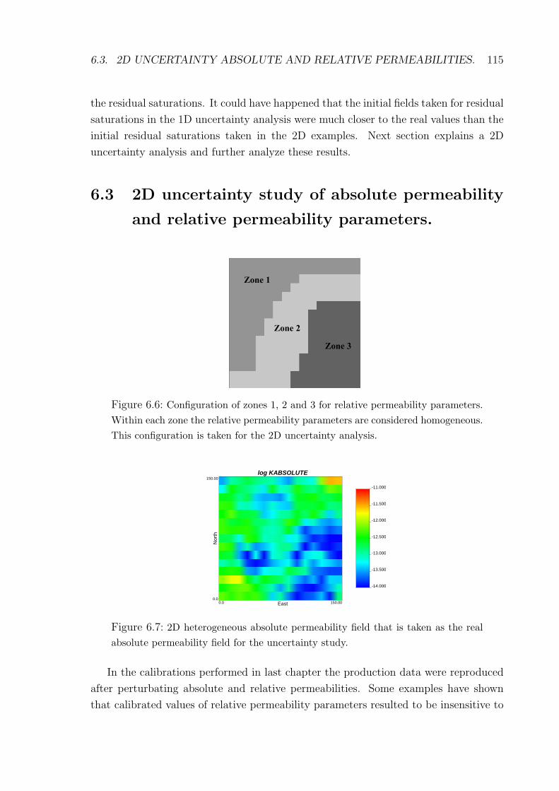
6.3. 2D UNCERTAINTY ABSOLUTE AND RELATIVE PERMEABILITIES. 115
the residual saturations. It could have happened that the initial fields taken for residual
saturations in the 1D uncertainty analysis were much closer to the real values than the
initial residual saturations taken in the 2D examples. Next section explains a 2D
uncertainty analysis and further analyze these results.
6.3 2D uncertainty study of absolute permeability
and relative permeability parameters.
Zone 1
Zone 2
Zone 3
Figure 6.6: Configuration of zones 1, 2 and 3 for relative permeability parameters.Within each zone the relative permeability parameters are considered homogeneous.This configuration is taken for the 2D uncertainty analysis.
log KABSOLUTE
East
Nor
th
0.0 150.000.0
150.00
-14.000
-13.500
-13.000
-12.500
-12.000
-11.500
-11.000
Figure 6.7: 2D heterogeneous absolute permeability field that is taken as the realabsolute permeability field for the uncertainty study.
In the calibrations performed in last chapter the production data were reproduced
after perturbating absolute and relative permeabilities. Some examples have shown
that calibrated values of relative permeability parameters resulted to be insensitive to

116 CHAPTER 6. UNCERTAINTY STUDY
saturations and pressures. On the other hand, the uncertainty analysis performed in
1D (last two sections) concludes that the uncertainty related with the end-points is
quite wide, while for residual saturations the inter-quantile range is very narrow. The
2D calibrations performed in chapter 5 suggest that also for residual saturations the
uncertainty range should be rather wide. In this section a 2D uncertainty analysis is
performed. The high computational cost required for each 2D calibration has limited
the number of realizations for the uncertainty analysis to 10 runs.
End-point krw
East
Nor
th
0.0 150.000.0
150.00
0.0
0.1000
0.2000
0.3000
0.4000
0.5000
0.6000
0.7000
0.8000
0.900
1.000
(a) k0rw
Srw
East
Nor
th
0.0 150.000.0
150.00
0.0
0.1000
0.2000
0.3000
0.4000
0.5000
0.6000
0.7000
0.8000
0.900
1.000
(b) Srw
End-point Kro
East
Nor
th
0. 0 150.000.0
150.00
0.0
0.1000
0.2000
0.3000
0.4000
0.5000
0.6000
0.7000
0.8000
0.900
1.000
(c) k0ro
Sro
East
Nor
th
0.0 150.000.0
150.00
0.0
0.1000
0.2000
0.3000
0.4000
0.5000
0.6000
0.7000
0.8000
0.900
1.000
(d) Sro
Figure 6.8: 2D values for k0rw, Srw, k0
ro and Sro given in three zones. They are the true valuesfor the 2D uncertainty study.
The problem configuration is similar to the examples shown in chapter 5. Different
geometry has been chosen for the zones that define the heterogeneity of relative per-
meability in order to reproduce a geology that would be closer to a real realization.
As in other cases, 3 zones of the domain are considered to have homogeneous relative
permeability parameters. These zones are numbered from 1 to 3 and their contour
limits are plotted in Figure 6.6. The true case is represented with absolute and relative

6.3. 2D UNCERTAINTY ABSOLUTE AND RELATIVE PERMEABILITIES. 117
SATURATIONS
East
Nor
th
0.0 150.000.0
150.00
0.0
0.1000
0.2000
0.3000
0.4000
0.5000
0.6000
0.7000
0.8000
0.900
1.000
PRESSURES
East
Nor
th
0.0 150.000.0
150.00
15000000.
16000000.
17000000.
18000000.
19000000.
20000000.
21000000.
22000000.
23000000.
24000000.
25000000.
(b) P
Figure 6.9: When introducing real parameters in the forward two-phase flow simulator thisis the saturation (a) and pressure (b) field obtained at the end of the simulation. These aresaturation and pressure fields corresponding to the true fields for the 2D uncertainty study.
permeability fields, graphed in Figures 6.7 and 6.8. The absolute permeability field, as
explained in former chapters, is constructed with GCOSIM3D simulation code. The
log-mean is equal to -13.0 and the variance is equal to 0.3. The field is isotropic and
spatial continuity can be described with a spherical variogram model of range equal to
60m. The porosity is equal to φ = 0.2. True absolute permeability values are assumed
to be known, and only relative permeability parameters are subjected to calibration.
The well configuration is the already used quarter five spot case. The same spatial
discretization used in former 2D simulations of 15x15 grid blocks (of 10x10m) is taken.
600 time steps of 4.8 hours are used for the time discretization. In this example the
injection well is situated in the upper right grid block of the domain and the production
well in the lower left grid block. The injection and production rates are equal to 2.5kg/s.
At the end of the forward simulation, for the last time step, the saturation and pressure
fields are given in Figure 6.9.
After 10 calibrations, statistical analysis has been applied to the ensemble of end-
points and residual saturations estimated. Likewise in the 1D uncertainty analysis,
these statistics were median, Q25 and Q75 interquantiles. The results, in comparison
with the real values, are graphed in Figures 6.10 and 6.11.
These graphs show a very narrow uncertainty range for the four parameters, which
do not envelope the real corresponding values. This result suggest that more calibra-
tions should be performed in order to get a wider range of different possible values, 10
calibrations is not enough to infer the probabilities corresponding to the output ensem-
ble. The results obtained in 1D, and the calibrated values given by the 2D examples

118 CHAPTER 6. UNCERTAINTY STUDY
Krw01 Krw02 Krw03 Kro01 Kro02 Kro03.000
.100
.200
.300
.400
.500
.600
.700
.800
.900
1.000
End-points calibration for the 3 zones
Q75
Real
Median
Q25
End-point zone
End
-poin
t re
lati
ve p
erm
eab
ilit
y
Figure 6.10: Uncertainty related with the end-points of water and oil relative per-meability curves for the 3 areas in which the domain is divided. Real values arerepresented with a red diamond and median with a light blue square. Probabilityvalues are calculated from 10 different calibrations in 2D.
Srw1 Srw2 Srw2 Sro1 Sro2 Sro3.000
.100
.200
.300
.400
.500
.600
.700
.800
.900
1.000
Residual sat. calibration for the 3 zones
Q75
Real
Median
Columna 17
Residual sat. zone
Resid
ual satu
rati
on
Figure 6.11: Uncertainty related with the water and oil residual saturations for the3 areas in which the domain is divided. Real values are represented with a reddiamond and median with a light blue square. Probability values are calculatedfrom 10 different 2D calibrations.
have point out the large uncertainty related with the end-point of relative permeabili-
ties. Even this uncertainty analysis performed in 2D gives smaller inter-quantile range
for the end-points, it is probably due to the few number of calibrations performed. To
solve this necessity the method should be improved in order to perform a higher number

6.3. 2D UNCERTAINTY ABSOLUTE AND RELATIVE PERMEABILITIES. 119
of calibrations much faster than in the computations run during this dissertation.
Fractional flow at production well
0.0
0.1
0.2
0.3
0.4
0.5
0.6
0 20 40 60 80 100 120Time (days)
fw
fw_truefw_medianfw_Q25fw_Q75
Figure 6.12: Evolution of fractional flow with time. The fw values are plotted forthe true parameters and the statics calculated from 10 different 2D calibrations.
The set of relative permeability values would correspond to 10 different water
breakthrough responses. This set of water saturations can also be used to study the
uncertainty in the production forecasts. Statistics can also be computed on the set of
10 saturation fields. The results, given in fractional flow terms, are plotted in Figure
6.12. The true curve (plotted in dark blue) in the production well (lower left corner)
corresponds to the fractional flow values in function of time. Statistical values are
computed from the 10 equivalent curves of the 10 calibrations, plotted in the same
Figure 6.12. It has been pointed out that more realizations should be run to obtain
a better uncertainty study, but these values give an idea of the behavior of the pro-
duction forecast. At the initial stages of the production upper and lower quantiles
envelope both median an real values. However, when the water production increases
its rate, the uncertainty range gives worse prediction. In any case, all the curves are
very close to each other indicating the good predictions that could be obtained by using
the inversion method described here.
All these results indicate that uncertainties related with the end-points of relative
permeability curves are higher than the uncertainties related with residual saturations.
However, the calibrated values for the 2D examples presented an important lack of
sensitivity of these parameters to saturation and pressure production data. Further
research is needed in order to improve the computational time to be able to perform
more simulations and more uncertainty analysis in different situations. The importance
of the heterogeneity in relative permeability functions has been marked during the

120 CHAPTER 6. UNCERTAINTY STUDY
tests shown in former chapters. The values and spatial distribution of these parameters
influence so much on the saturation shock front distribution that more attention should
be paid to the role of these parameters in multiphase flow simulations.

Chapter 7
Conclusions and further research
7.1 Conclusions
The main objective of this dissertation is to take into account relative permeability
heterogeneities in inverse two-phase flow modeling for reservoir characterization pur-
poses. After performing a literature review (chapter 2) it was found out that, to the
best of our knowledge, there is an important gap in inverse two-phase flow techniques
in what refers to the role of relative permeabilities. Then, the different possibilities
to implement the heterogeneities of relative permeability curves in forward two-phase
flow simulators were analyzed (chapter 3). A new tool to carry out inverse modeling of
relative permeability parameters was developed (chapter 4). Once the tool was ready
to use, different examples in 2D have shown the applicability of the method (chapter
5) and uncertainty analysis were performed (chapter 6). It is the aim of this disserta-
tion to investigate the influence of relative permeabilities on the behavior of dynamic
variables in the reservoir. From the research done, the principal conclusions that can
be extracted are:
1. A literature research showed that it is very common to perform stochastic inverse
modeling in order to characterize the heterogeneity of absolute permeability. The
majority of the references checked assume homogeneous relative permeability
curves when multiphase flow is subjected to inverse modeling. However, some
approaches consider heterogeneous relative permeability. The few works that es-
timate relative permeability parameters with inverse modeling, considering these
functions to be heterogeneous, are applied to core sample scale cases and not to
reservoir scale. In these studies some of the parameters that define the relative
permeability functions are chosen to be estimated by history matching processes.
Furthermore, the conclusions given by these research works reveal the impor-
121

122 CHAPTER 7. CONCLUSIONS AND FURTHER RESEARCH
tance of the estimation of relative permeability functions. In general, there is
not a technique to inverse model relative permeability functions considering their
heterogeneity within the reservoir, at reservoir scale.
2. It has been possible to develop and implement a code that calibrates simulta-
neously relative and absolute permeability functions to historical data. In this
code relative permeabilities are assumed to be function of saturation, and are
expressed as power functions. Four parameters were chosen to characterize the
relative permeability curves: the two end-points of the curves and the residual
saturations. These parameters are subjected to calibration to dynamic varia-
bles such as saturations and pressures. The method not only allows to estimate
relative permeability functions, another important contribution is that the cali-
bration of relative permeability parameters is performed simultaneously with the
calibration of absolute permeability when absolute and relative permeabilities are
considered to be spatially variable.
3. Inverse calibration has been computed following the ideas given by the Sequential
Self-Calibrated method. This methodology allows to reduce the parameter space
for the calculation of perturbations, making the process faster. The concept of
master point perturbations has been successfully implement in the two-phase flow
simulation showing the advantages of this method not only in single phase flow
simulations, but also when the concept of relative permeability is necessary to
define the flow equations.
4. It has been shown that the code can be successfully applied to different kind of
1D and 2D cases. Different type of data are integrated with the inversion met-
hod developed. Static variable measurements such as absolute permeabilities are
considered in the examples shown. Dynamic variables as saturations and pres-
sures are integrated through the iterative inversion method, keeping the static
variable measurements. The possibilities given by the integration of soft data,
as the seismic information, are shown in one of the examples run. 4D seismic
information can enormously improve the estimation of the absolute and rela-
tive permeabilities at the same time that the uncertainty related with calibrated
relative permeability parameters seems to be reduced.
5. All the inverse modeling examples, and even the forward simulations, reveal that
the heterogeneity of the relative permeability functions can dramatically change
the dynamic behavior of the reservoir. When oil is displaced by injected water,
this influence of relative permeabilities spatial variation is very important for

7.2. SUGGESTIONS FOR FURTHER RESEARCH 123
the saturation shock front. This means that if the relative permeabilities (or
fractional flow, which is a variable dependent on relative permeabilities) are going
to be estimated it is not sufficient to calibrate them to pressure data, saturations
must also be considered to get a real estimation.
6. The uncertainty analysis studied in 1D has shown that uncertainties related with
the end-points of water and oil relative permeability curves are quite wide. These
uncertainties are reduced if instead of just consider saturation measurements,
pressures are also included in the objective function. The uncertainties related
with residual saturations in this 1D analysis resulted very narrow, as well as for
the estimated absolute permeabilities.
7. In 2D, the uncertainty analysis gives results similar with the 1D uncertainty
analysis. The number of realizations performed in 2D was limited by the compu-
tational cost, and more runs would be necessary to perform a complete analysis
as it has been done in 1D. The ensemble of water breakthrough values allows to
perform an uncertainty study in the production predictions. Better production
forecasts are obtained in the first stages of the exploitation.
All these points resume the principal conclusions of the research done in this dis-
sertation, and give an answer to the objectives that were proposed at the beginning of
the research work (explained in chapter 1). However, there were parts of the work that
did not result as it was expected, and new options have appeared during the research.
Thus, further research must be continued to investigate in this direction and to facili-
tate the creation of a more practical tool to inverse estimate relative permeabilities at
reservoir scale.
7.2 Suggestions for further research
The following issues deserving further research have been identified:
• The difficulty of the method is the high computational cost that the method re-
quires at each iteration. The forward 2D problem requires a considerable time to
be run, and this is one of the main reasons why at each iteration so much time
was needed. Thus more research has to be conducted in what refers to forward
modeling, especially in the area of numerical solvers for non linear differential
system of equations. One of the possible solutions would be to apply streamline
simulators and fractional flow formulation. Making the forward method compu-
tationally faster, each iteration could be speed up, and the inverse method could
be applied to higher domains and discretizations.

124 CHAPTER 7. CONCLUSIONS AND FURTHER RESEARCH
• Altough the use of the concept of master points reduces the number of para-
meters in which the perturbations must be computed, there is still another area
which needs further research to obtain less computational time: the optimization
algorithm used in the iterative inversion. Presently, the inverse method uses a
numerical approach of the gradient of the objective function. It also uses gra-
dient approaches to solve the optimization process. These approximations are
valid, but it would be desirable to implement other approximations in order to
make the process faster. One possible solution for further research it would be
the implementation of the sensitivity equations to use a second order method to
perform the optimization during the inversion. As the forward two-phase flow
simulator, the optimization algorithm needs an improvement in order to make
possible the study of higher dimensional fields with more discretization.
• Other possibility to increase the performance of the method it would be the
study of parallel computing advantages to speed up the CPU cost. These new
techniques offer the possibility to get good computational times in complex non
linear problems as the one study here.
• The information used in the examples shown in this dissertation has consisted
in absolute permeability data, saturations and pressures. The use of relative
permeability measurements was not explored in this work, and further research
to include relative permeability available data should be considered.
• The use of seismic information has shown the improvements that can be obtained
in the model. The very recent availability of new sensors to measure pressure
and temperature downhole in a permanent way is still on research and develop in
order to build a new pressure sensor. The pressure data acquired with this kind
of new techniques is an important potential application of the inverse method
presented here, very similar to the seismic 4D data application.
• As it is available an inverse code for the numerical solver used during this disser-
tation (TOUGH code) called ITOUGH, it would be very interesting to compare
the proceduce presented here with the inverse code ITOUGH. A modification
of the code to take into account heterogeneities of the relative permeabilities
parameters for the inversion would have to be done.
• If the improvement in the computational cost of the process is reached, the next
step that should be considered is the application of the method to a real case.
The examples and studies shown in this dissertation are created synthetically
and still remains to show how the estimation of relative permeability curves by

7.2. SUGGESTIONS FOR FURTHER RESEARCH 125
inverse two-phase flow can improve the characterization of the reservoir in a real
case.

126 CHAPTER 7. CONCLUSIONS AND FURTHER RESEARCH

Appendix A
Buckley-Leverett solution
The formulation of the 1D two-phase immiscible flow with the fractional flow is descri-
bed in chapters 2 and 3. The equation that must be solved is (equation (3.12)):
φ∂Sw
∂t+ uT
∂fw
∂Sw
∇Sw = fwqT − qw
To solve this equation Bukley y Leverett assumed the following initial and boundary
conditions:
Sw(x, 0) = SwI , x ≥ 0
Sw(0, t) = SwJ , t ≥ 0(A.1)
Initially the medium has a saturation equal to SwI . At the origin position x = 0
water is injected with constant rate qw, keeping constant the saturation at the injection
well, equal to SwJ . At origin and initial time, t = x = 0, all the values for Sw are
possible ranging between SwI and SwJ .
Assuming that there are not injection nor production terms, the equation (3.12)
and (A.1) can be rewritten in a simpler way (adimensional):
(∂Sw
∂tD
)+
(∂fw
∂Sw
) (∂Sw
∂xD
)= 0 (A.2)
Sw(xD, 0) = SwJ , xD ≥ 0 (A.3)
Sw(0, tD) = SwJ , tD ≥ 0 (A.4)
where xD and tD are adimensional variables equal to:
127

128 APPENDIX A. BUCKLEY-LEVERETT SOLUTION
xD = xL
tD =∫ t
0uT dtφL
xD is the adimensional space variable and tD is the adimensional time variable. L is
the total length of the porous medium in the direction of x. In these equations uT
can be function of time but it cannot be function of position because incompressibility
has been assumed. Moreover, dfw
dSwis the total derivative because fw is function of Sw
(unique dependent variable).
Equation (A.2) is a differential equation of first order partial derivatives, the unique
dependent variable is Sw = Sw(x, t) because ∂fw
∂Swis function of Sw. This equation can
be solved with numerical methods or with the method of characteristics (Marle, 1981).
Multiplying and dividing by the transversal section A, the adimensional time can
also be expressed as:
tD =
∫ t
0
Audt
AφL=
∫ t
0
QT dt
Vp
(A.5)
where QT is the volumetric flux rate and Vp is the porous volume. tD is the total
volume injected until time t divided by the total porous volume.
Starting from equation (A.2), saturation Sw can be written in a differential form:
dSw =
(∂Sw
∂xD
)tD
dxD +
(∂Sw
∂tD
)xD
dtD (A.6)
The velocity vsw can be deduced from this equation (A.6). For a point at constant
saturation Sw in the space xD − tD the velocity is equal to:(dxD
dtD
)Sw
= −(∂Sw/∂td)xD
(∂Sw/∂xD)tD
≡ vSw (A.7)
This is the specific velocity of saturation Sw because it has been normalized with u/φ.
Applying the equation (A.7) to equation (A.2) the result is:
vSw =dfw
dSw
(A.8)
The meaning of the equation (A.8) is that the specific velocity of constant saturation
Sw is equal to the derivative of the fractional flow curve at this point Sw of the curve
fw −Sw. This equation is the solution of the one dimensional problem of displacement
of petroleum with water, and can be used to predict the rate of displacement of the
shock front. Selecting different Sw between SwI and SwJ , the curve Sw(xD, tD) can be
built. Fractional flow, fw, is a function of relative permeabilities, thus a function of
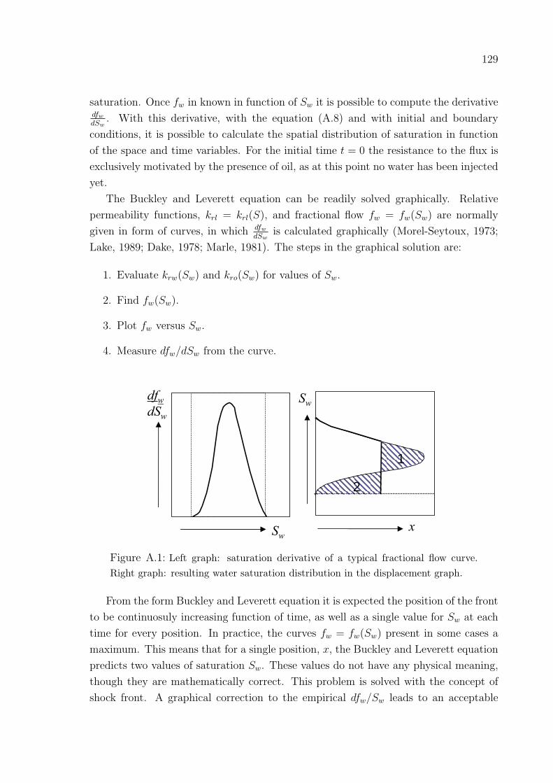
129
saturation. Once fw in known in function of Sw it is possible to compute the derivativedfw
dSw. With this derivative, with the equation (A.8) and with initial and boundary
conditions, it is possible to calculate the spatial distribution of saturation in function
of the space and time variables. For the initial time t = 0 the resistance to the flux is
exclusively motivated by the presence of oil, as at this point no water has been injected
yet.
The Buckley and Leverett equation can be readily solved graphically. Relative
permeability functions, krl = krl(S), and fractional flow fw = fw(Sw) are normally
given in form of curves, in which dfw
dSwis calculated graphically (Morel-Seytoux, 1973;
Lake, 1989; Dake, 1978; Marle, 1981). The steps in the graphical solution are:
1. Evaluate krw(Sw) and kro(Sw) for values of Sw.
2. Find fw(Sw).
3. Plot fw versus Sw.
4. Measure dfw/dSw from the curve.
Sw
x
1
2
Sw
dfwdSw
Figure A.1: Left graph: saturation derivative of a typical fractional flow curve.Right graph: resulting water saturation distribution in the displacement graph.
From the form Buckley and Leverett equation it is expected the position of the front
to be continuosuly increasing function of time, as well as a single value for Sw at each
time for every position. In practice, the curves fw = fw(Sw) present in some cases a
maximum. This means that for a single position, x, the Buckley and Leverett equation
predicts two values of saturation Sw. These values do not have any physical meaning,
though they are mathematically correct. This problem is solved with the concept of
shock front. A graphical correction to the empirical dfw/Sw leads to an acceptable

130 APPENDIX A. BUCKLEY-LEVERETT SOLUTION
solution. A value of dfw/dSw is chosen such that the areas 1 y 2 (look Figure A.1)
are equal. The derivative curve is truncated so the value of x is the same for all
Sw below the threshold. This implies an abrupt jump in Sw at a specific x-position.
This is observed in practice and is called the shock front. This implies that there are
discontinuous changes of saturation. Strictly speaking the discontinuities do not exist
in nature because there is always a diffusive effect that spreads the discontinuity effect.
Although this phenomenon exists, the role that discontinuity has in the displacement
is fundamental for the theory of the fractional flow, where the diffusive mechanisms are
ignored. The solution given by Buckley and Leverett is a good approximation when
capillary effects are neglected and the flow rates are high (Bear, 1972).

Appendix B
Sensitivity equations for the
fractional flow formulation
In chapter 4 it was described how the perturbation of the master points can be calcula-
ted numerically. The gradient vector containing the partial derivatives of the objective
function with respect to perturbations at the master point locations must be calcu-
lated. In this appendix the fractional flow formulation given in chapter 3 is taken to
describe another way to compute the perturbations, with adjoint states. The following
steps are similar to the explanation given in Hendricks-Frassen (2001).
B.1 Adjoint states
The fracional flow formulation has the water saturations Sw as the state variables.
There are N × T state variables, where N is the total number of discretization nodes
and T is the number of times in which the simulation time is discretized. Let’s define
the vector {p}, with dimension M containing all the parameters to be calibrated. The
water saturations and the parameters are related through N × T state equations:
Ψ({Sw}, {p}) = 0 (B.1)
State equations can be expressed with the fractional flow formulation, or with other
approaches mentioned in the literative review as the two pressures method. Let’s take
for this case the fractional flow approach. The matix form of the two-phase flow
equation is (equation (??)):
[A]({St+1} − {St}
)= {Qt+1} (B.2)
131

132 APPENDIX B. SENSITIVITY EQUATIONS
where [A] is N ×N matrix and {Q} and {S} are vectors of dimension N . Ai elements
are equal to:
Ai =Vi
∆t(B.3)
and Qti:
Qti = QT f t+1
w,i−1 −Qt+1w,i (B.4)
The state equations for two sucessive time steps can be written as:
{Ψt} = [A]({St} − {St−1}
)− {Qt} = 0 (B.5)
{Ψt+1} = [A]({St+1} − {St}
)− {Qt+1} = 0 (B.6)
The Lagrangian of the objetive function to be minimized buject to the constrains
B.5 and B.6 is:
= = J + {λ}′{Ψ} (B.7)
where λ is a vector of length N × T , which elements are the Lagrange multipliers,
also called adjoint states. {λ}′ represents the transpose of the vector {λ}′. For each
of the times in shcih teh adjoint state equation is solved a vector {λ} of dimensions
N is estimated. The Lagrange multipliers obtained for the state {Ψt} are {λt}, the
Lagrange multiplier for state {Ψt+1} are {λt+1}, and similarlty for the following time
steps.
The derivatives of the Lagrangian with respect the perturbation parameters, {p},are given by the equation:
d=d{p}
=dJ
d{p}=
∂J
∂{p}+
∂J
∂{Sw}∂{Sw}∂{p}
+ {λ}′(
∂{Ψ}∂{p}
+∂{Ψ}∂{Sw}
∂{Sw}∂{p}
)(B.8)
This derivatives are similar to the derivatives of the objective function with respect the
perturbation parameters. Equation (B.8) can be rearrange as:
dJ
d{p}=
∂J
∂{p}+
(∂J
∂{Sw}+ {λ}T ∂{Ψ}
∂{Sw}
)∂{Sw}∂{p}
+ {λ}T ∂{Ψ}∂{p}
(B.9)
The adjoing state is taken as the solution of the expression:
∂J
∂{Sw}+ {λ}T ∂{Ψ}
∂{Sw}= 0 (B.10)
which makes that equation (B.9) can be simplified resulting:

B.2. CALCUATION OF THE ADJOINT STATES 133
dJ
d{p}=
∂J
∂{p}+ {λ}T ∂{Ψ}
∂{p}(B.11)
The adjoint states vector is estimated by solving equation (B.8). The result can be
used to compute the gradient of the objective function given by equation (B.11).
B.2 Calculation of the adjoint states for the frac-
tional flow formulation
The objective function has been defined in chapter 4. For the fractional flow formula-
tion let’s consider that only water saturation measurements are available, and that the
weighting terms are equal to 1. Then, the objective function is:
J =Ts∑t=1
Ns∑i=1
(St,SIM
w,i − St,MEASw,i
)2
(B.12)
Ns is the number of water saturation measurements and Ts the number of times in
which the water saturation data are taken. Exponents SIM and MEAS refer to
simulated and measured values.
With this definition of the objective function, the derivatives with respect the state
variables, that appear in equation (B.10), can be expressed as:
∂J
∂{Stw}
= 2Ts∑t=1
Ns∑i=1
(St,SIM
wi − St,MEASwi
)(B.13)
The derivatives of the state equation with respect the water saturation in the time
step t (second term in equation (B.10)) are not equal to zero only for the times t and
t + 1:
∂{Ψt}∂{St
w}=
([A]− ∂{Qt}
∂{Stw}
)(B.14)
∂{Ψt+1}∂{St
w}=
(−[A]− ∂{Qt+1}
∂{Stw}
)(B.15)
Combining the equations (B.13) and (B.15) with equation (B.10) the adjoint state
equation is:
2Ts∑t=1
Ns∑i=1
(St,SIM
wi − St,MEASwi
)+ {λt}′
([A]− ∂{Qt}
∂{Stw}
)+{λt+1}′
(−[A]− ∂{Qt+1}
∂{Stw}
)= 0
(B.16)

134 APPENDIX B. SENSITIVITY EQUATIONS
Remember that Qti = QT f t+1
w,i−1 − Qt+1w,i , hence the partial derivatives ∂{Qt}
∂{Stw} and
∂{Qt+1}∂{St
w} are equal to zero. The adjoint state equation simplies to the following form:
2Ts∑t=1
Ns∑i=1
(St,SIM
wi − St,MEASwi
)+ {λt}′ ([A]) + {λt+1}′ (−[A]) = 0 (B.17)
which rearranging terms is:
[A]({λt+1}′ − {λt}′
)= 2
Ts∑t=1
Ns∑i=1
(St,SIM
wi − St,MEASwi
)(B.18)
This is the adjoing state equation, which has a similar form to the flow equation
expressed with the fractional flow formulation. In this equation (B.18) the unknowns
are the adjoint states and the independent term is not function of fractional flow. This
similarity is normally used in order to reduce the time of calcuation for the coefficients
of the system of equations.
B.3 Calculation of the gradient of J using the ad-
joint states
Once the adjoint states are computed following the steps given in former sectioin, it is
possible to used them to calculate the gradient of the objective function with equation
(B.11). The derivatives that appear in that equation can be expressed as follows:
∂J
∂{p}= 0 (B.19)
∂{Ψt}∂{p}
=∂[A]
∂{p}({St
w} − {St−1w }
)− ∂{Qt}
∂{p}(B.20)
As all the element of [A] are constants, its derivative with respect the parameters
is zero. Then, it is possible to solve the equation (B.11) calculating:
∂{Ψt}∂{p}
= −∂{Qt}∂{p}
(B.21)
With the definition of Qti:
∂Qti
∂pk
= QT
∂f t+1w,i−1
∂pk
(B.22)
where f t+1w,i is function of pi. Those pi are the paremeter values in all the nodes, that
are expressed as a linear combination of the parameters in a few points (master points)
pk:

B.3. CALCULATION OF THE GRADIENT OF J 135
pi =∑
k
eki pk (B.23)
eki could be, for exmple, the ordinary kriging coefficients when pi is estimated with
the values at the master points, pk. If the parameters are expressed in this way, the
derivatives of the fractional flow with respect the parameters are:
∂Qti
∂pk
= QT
∂f t+1w,i−1
∂pi
∂pi
∂pk
= QT
∂f t+1w,i−1
∂pi
∂pi
∂pk
(B.24)
where:
∂pi
∂pk
= eki (B.25)
∂f t+1w,i−1
∂pican be deduced from the expression of fw in potential form:
fw =1
1 + µwk0ro
µok0rw
(1−S)no
Snw
where S is the water reduced saturation:
S =Sw − Srw
1− Srw − Sro
If the perturbation parameter is k0rw the derivative is:
∂fw
∂k0rw
=1
k0rw
µwk0ro
µok0rw
(1−S)no
Snw(1 + µwk0
ro
µok0rw
(1−S)no
Snw
)2 =µwk0
ro
µok02rw
(1− S)no
Snwf 2
w
This derivatives for all the perturbation parameters have to be introduced in equa-
tion (B.24), in order to get the derivatives of the state equation (B.21). This derivatives
are sustituted in equation (B.11) to finally get the derivatives of the objective function
with respect the perturbation parameters.

136 APPENDIX B. SENSITIVITY EQUATIONS

Bibliography
[1] R.C. Abbaspour, M.T. van Genuchten, R. Schulin, and E. Schlappi. A sequential
uncertainty domain inverse procedure for estimating subsurface flow and trans-
port parameters. Water Resources Research, 33(8):1879–1892, 1997.
[2] L. M. Abriola and G. F. Pinder. A multiphase approach to the modelling of
porous media contamination by organic compounds 1. Equation development.
Water Resources Research, 21(1):11–18, 1985.
[3] L. M. Abriola and G. F. Pinder. A multiphase approach to the modelling of
porous media contamination by organic compounds 2. Numerical simulation.
Water Resources Research, 21(1):19–26, 1985.
[4] L. M. Abriola and K. Rathfelder. Mass balance errors in modelling two-phase
inmiscible flows: causes and remedies. Advances in Water Resources Research,
16:223–239, 1993.
[5] B. Agarwal and J. Blunt. A full-physics, streamline-based method for history
matching performance data of a north sea field. SPE 66388, 2001.
[6] S. Akin. Estimation of fracture relative permeabilities from unsteady state core-
floods. Petroleum Science and Engineering, 30:1–14, 2001.
[7] F. O. Alpak, C. Torres-Verdın, and K. Sepehrnoori. Numerical simulation and
inversion of pressure data acquired with permanent sensor. SPE 71612, 2001.
[8] M. Armstrong and P.A. Dowd, editors. Geostatistical simulations. Proceedings
of the Geostatistical Simulation Workshop, Fontainebleau, France, 27-28 May,
1993, Kluwer Academic Publishers, Dordrecht, Holland, 1994.
[9] H. Ates and M. Kelkar. Incorporation of two-phase production data into reservoir
characterization. SPE Annual Technical Conference and Exhibition hel in New
Orleans, Loisiana, 27-30 September, 1998.
137
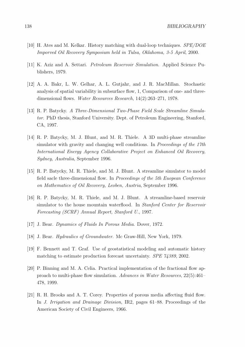
138 BIBLIOGRAPHY
[10] H. Ates and M. Kelkar. History matching with dual-loop techniques. SPE/DOE
Imporved Oil Recovery Symposium held in Tulsa, Oklahoma, 3-5 April, 2000.
[11] K. Aziz and A. Settari. Petroleum Reservoir Simulation. Applied Science Pu-
blishers, 1979.
[12] A. A. Bakr, L. W. Gelhar, A. L. Gutjahr, and J. R. MacMillan. Stochastic
analysis of spatial variability in subsurface flow, 1, Comparison of one- and three-
dimensional flows. Water Resources Research, 14(2):263–271, 1978.
[13] R. P. Batycky. A Three-Dimensional Two-Phase Field Scale Streamline Simula-
tor. PhD thesis, Stanford University. Dept. of Petroleum Engineering, Stanford,
CA, 1997.
[14] R. P. Batycky, M. J. Blunt, and M. R. Thiele. A 3D multi-phase streamline
simulator with gravity and changing well conditions. In Proceedings of the 17th
International Energy Agency Collaborative Project on Enhanced Oil Recovery,
Sydney, Australia, September 1996.
[15] R. P. Batycky, M. R. Thiele, and M. J. Blunt. A streamline simulator to model
field sacle three-dimensional flow. In Proceedings of the 5th Euopean Conference
on Mathematics of Oil Recovery, Leoben, Austria, September 1996.
[16] R. P. Batycky, M. R. Thiele, and M. J. Blunt. A streamline-based reservoir
simulator to the house mountain waterflood. In Stanford Center for Reservoir
Forecasting (SCRF) Annual Report, Stanford U., 1997.
[17] J. Bear. Dynamics of Fluids In Porous Media. Dover, 1972.
[18] J. Bear. Hydraulics of Groundwater. Mc Graw-Hill, New York, 1979.
[19] F. Bennett and T. Graf. Use of geostatistical modeling and automatic history
matching to estimate production forecast uncertainty. SPE 74389, 2002.
[20] P. Binning and M. A. Celia. Practical implementation of the fractional flow ap-
proach to multi-phase flow simulation. Advances in Water Resources, 22(5):461–
478, 1999.
[21] R. H. Brooks and A. T. Corey. Properties of porous media affecting fluid flow.
In J. Irrigation and Drainage Division, IR2, pages 61–88. Proceedings of the
American Society of Civil Engineers, 1966.

BIBLIOGRAPHY 139
[22] S.E. Buckely and M.C. Leverett. Mechanism of fluid displacement in sands.
Transactions AIME, 146:107–116, 1942.
[23] J.E. Capilla, J.J. Gomez-Hernandez, and A. Sahuquillo. Stochastic simulation of
transmissivity fields conditional to both transmissivity and piezometric data, 2,
Demonstration on a synthetic aquifer. Journal of Hydrology, 203(1–4):175–188,
1997.
[24] J.E. Capilla, J.J. Gomez-Hernandez, and A. Sahuquillo. Stochastic simulation of
transmissivity fields conditional to both transmissivity and piezometric data, 3,
Application to the WIPP site. Journal of Hydrology, 207(3–4):254–269, 1998.
[25] J. Carrera and S. P. Neuman. Estimation of aquifer parameters under transient
and steady state conditions, 1, Maximum likelihood method incorporating prior
information. Water Resources Research, 22(2):199–210, 1986.
[26] J. Carrera and S. P. Neuman. Estimation of aquifer parameters under transient
and steady state conditions, 2, Uniqueness, stability, and solution algorithms.
Water Resources Research, 22(2):211–227, 1986.
[27] J. Carrera and S. P. Neuman. Estimation of aquifer parameters under transient
and steady state conditions, 3, Application to synthetic and field data. Water
Resources Research, 22(2):228–2427, 1986.
[28] R. D. Carter, L. F. Kemp, A. C. Pierce, and D. L. Williams. Permformance
matching with constrains. Society of Petroleum Engineers Journal, 14(4):187–
196, 1974.
[29] M. A. Celia, H. Rajaram, and L. A. Ferrand. A multi-scale computational model
for multiphase flow in porous media. Adv. Water Resources, 16:81–92, 1993.
[30] M. A. Cella, E. T. Bouloutas, and R. L. Zarba. A general mass-conservative
numerical solution for the unsaturated flow equations. Water Resources Research,
26(7):1483–1496, 1990.
[31] Z. Chen, M. Espedal, and R. E. Ewing. Continuous-time finite element analysis of
multiphase flow in groundwater hydrology. Applications of Mathematics, 40:203–
226, 1995.
[32] J.-P. Chiles and P. Delfiner. Geostatistics. Modeling spatial uncertainty. John
Wiley and Sons Inc., New York, 1999.

140 BIBLIOGRAPHY
[33] L. Chu, A. C. Reynolds, and D. S. Oliver. Computation of sensitivity coeffi-
cients for conditioning the permeability field to well-test pressure data. In Situ,
19(2):179–223, 1995.
[34] K. H. Coats, R. L. Nielsen, M. H. Terhune, and A. G. Weber. Simulation of
three-dimensional, two-phase flow in oil and gas reservoirs. Transactions AIME,
240:377–388, 1967.
[35] G. Dagan. Stochastic modeling of groundwater flow by unconditional and
conditional probabilities, 2, The inverse problem. Water Resources Research,
21(4):573–578, 1985.
[36] G. Dagan. Statistical theory of groundwater flow and transport: Pore to labora-
tory, laboratory to formation, and formation to regional scale. Water Resources
Research, 22(9):120S–134S, 1986.
[37] G. Dagan and Y. Rubin. Stochastic identification of recharge, transmissivity and
storativity in aquifer unsteady flow: a quasi-steady approach. Water Resources
Research, 24(10):1698–1710, 1988.
[38] H.K. Dahle, M.S. Espedal, R.E. Ewing, and O. Saevareid. Characteristic adaptive
subdomain methods for reservoir flow problems. Numerical Methods for Partial
Differential Equations, 6:279–309, 1990.
[39] L. P. Dake. Fundamentals of Reservoir Engineering. Elsevier, New York, 1978.
[40] A. Datta-Gupta, L. W. Lake, and G. A. Pope. Characterizing heterogeneous
permeable media with spatial statistics and tracer data using sequential simulated
annealing. Math Geol, 27(6):763–787, 1995.
[41] G. de Marsily. Quantitative Hydrogeology. Academic Press, 1986.
[42] G. de Marsily, G. Lavedau, M. Boucher, and G. Fasanino. Interpretation of inter-
ference test in a well field using geostatistical techniques to fit the permeability
distribution in a reservoir model. In G. W. Verly, M. David, A. G. Journel, and
A. Marechal, editors, Geostatistics for Natural Resources Characterization, pa-
ges 831–849. Proceedings of the NATO Advanced Study Institute, South Lake
Tahoe, California, September 6-17, D. Reidel, Dordrecht, Holland, 1984.
[43] C.V. Deutsch. Geostatistical Reservoir Modeling. Oxford University Press, New
York, first edition, 2002.

BIBLIOGRAPHY 141
[44] J. Jr. Douglas. Finite difference method for two-phase incompressible flow in
porous media. SIAM Journal of Numerical Analysis, 20:681–696, 1983.
[45] J. Jr. Douglas, D. W. Peaceman, and H. H. Jr. Tachford. A method for calculating
multi-dimensional immiscible displacement. Transactions AIME, 216:297–306,
1956.
[46] F. A. L. Dullien. Porous Media Fluid Transport and Pore Structure. Academic
Press, New York, 1979.
[47] R.E. Ewing. Simulation of multiphase flows in porous media. Transport in Porous
Media, 6:479–499, 1991.
[48] R. W. Falta, K. Pruess, S. Finsterle, and A. Battistelli. T2voc user’s guide.
Technical Report LBL-36400, Enerst Orlando Lawrence Berkeley National La-
boratory, Berkeley, 1995.
[49] C. R. Faust. Transport of immiscible fluids within and below the unsaturated
zone: a numerical model. Water Resources Research, 21(4):587–596, 1985.
[50] S. Finsterle and K. Pruess. Optimizing multiphase aquifer remediation using
itough2. Report LBL-36088, Lawrence Berkeley Laboratory, Berkeley, CA., 1994.
[51] S. Finsterle and K. Pruess. Solving the estimation-identification problme in two-
phase flow modeling. Water Resources Research, 31(4):913–924, 1995.
[52] F. J. T. Floris, M. D. Bush, M. Cuypers, F. Roggero, and A.-R. Syversveen. Com-
parison of production forecast uncertainty quantification methods: An integratd
study. Petroleum Geoscience, 7:S87–S96, 2001.
[53] F.J.T. Floris and C.F.M.Bos. Quantification of uncertainty reduction by condi-
tioning to dynamic production data. In Proceedings of European Conference on
the Mathematics of Oil Recovery, Peebles, Scotland, 8-11 September, 1998.
[54] P. A. Forsyth, A. J. A. Unger, and E. A. Sudicky. Nonlinear iteration methods
for nonequilibrium multiphase subsurfase flow. Advances in Water Resources,
18:25–38, 1995.
[55] P. A. Forsyth, Y. S. Wu, and K. Pruess. Robust numerical methods for saturated-
unsaturated flow with dry intial conditions in heterogeneous media. Advances in
Water Resources, 18:25–38, 1995.

142 BIBLIOGRAPHY
[56] R.A. Freeze. A stochastic-conceptual analysis of one-dimensional groundwater
flow in nonuniform heterogeneous media. Water Resources Research, 11(5):725,
741 1975.
[57] P. Frykman and H.F. Lindgaard. Dynamic upscaling of relative permeability in
chalk. Technical Report 1997/145, Geological survey of Denmark and Greenland,
1997.
[58] L.W. Gelhar. Stochastic subsurface hydrology from theory to application. Water
Resources Research, 22(9):135S–145S, 1986.
[59] J. Gomez-Hernandez, A. Sahuquillo, and J.E. Capilla. Stochastic simulation of
transmissivity fields conditional to both transmissivity and piezometric data. 1.
Theory. Journal of Hydrology, 203(1-4):162–174, 1997.
[60] J.J. Gomez-Hernandez and A.G. Journel. Joint simulation of multiGaussian
random variables. In Amilcar Soares, editor, Geostatistics Troia ’92, volume 1,
pages 85–94. Kluwer, 1993.
[61] P. Goovaerts. Geostatistics for Natural Resources Evaluation. Oxford University
Press, New York, 1997.
[62] A. A. Grimstad, K. Kolltveit, J. E. Nordtvedt, A. T. Watson, T. Mannseth, and
A. Sylte. The uniqueness and accuracy of porous media multiphase properties
estimated from displacement experiments. In Proceedings of the International
Symposium of the Society of Core Analysis, September 1997.
[63] P. Grindrod and M. D. Impey. Channeling and fickian dispersion in fractal
simulated porous media. Water Resources Research, 29(12):4077–4089, 1993.
[64] D. Guerillot and F. Roggero. Matching the future for the evaluation of extreme
reservoir development scenarios. In 8th European Symposium on Improved Oil
Recovery, Vienna, Austria, 15-17 May, 1995.
[65] A. Gutjahr, S. Hatch, and B. Bullard. Conditional simulation and contaminant
flow modeling: effects of linearization. Technical Completion Report Project
Number: WER-91-08, New Mexico Institute of Mining and Technology, 1993.
[66] A. Gutjahr, S. Hatch, and B. Bullard. Conditional simulation and contaminant
flow modeling: effects of linearization. Technical Completion Report Project
Number: WER-91-08, New Mexico Institute of Mining and Technology, 1994.

BIBLIOGRAPHY 143
[67] A. L. Gutjahr, L. W. Gelhar, A. A. Bakr, and J. R. MacMillan. Stochastic
analysis of spatial variability in subsurface flows. 2. Evaluation and application.
Water Resources Research, 14(5):953–959, 1978.
[68] A.L. Gutjahr. Fast fourier transforms for random field generator. Technical Com-
pletion Report A-R58-2690R, New Mexico Institute of Mining and Technology,
1989.
[69] S. Hanna and T.C. Jim Yeh. Estimation of co-coditional moments of trans-
missivity, hydraulic head, and velocity fields. Advances in Water Resources,
22(1):87–95, 1998.
[70] C. F. Harvey and S. M. Gorelick. Mapping hydraulic conductivity: Sequential
conditioning with measurements of solute arrival time, hydraulic head, and local
conductivity. Water Resources Research, 31(7):1615–1626, 1995.
[71] J.J. Hastings, A.H. Muggeridge, and M.J. Blunt. A new streamline method for
evaluating uncertainty in small-scale, two-phase flow properties. SPE 66349,
2001.
[72] B. K. Hegstad and H. Omre. Uncertainty assessment in history matching and
forecasting. In Baafi and Schofield, editors, Fifth International Geostatistics
Congress, Wollongong. Kluwer, 1997.
[73] B. K. Hegstad and H. Omre. Reservoir characterization integrating well ober-
vations, seismic data and producting history. Prepints Statistics no. 11/1998,
Deparment of mathmatical sciences, NTNU, Trondheim, Norway, 1998.
[74] B. K. Hegstad, H. Omre, H. Tjelmeland, and K. Tyler. Stochastic simulation and
conditioning by annealing reservoir description. In M. Armstrong and P. Dowd,
editors, Geostatistical Simulation, pages 43–55. Kluwer, 1994.
[75] H. J. Hendricks-Franssen. Inverse Stochastic Modelling of Groundwater Flow and
Mass Transport. PhD thesis, Universidad Politecnica de Valencia, Spain, 2001.
[76] D. Higdon, H. Lee, and Z. Bi. A bayesian approach to characterizing uncertainty
in inverse problems using coarse and fine-scale information. IEEE Transactions
on signal proceesing, 50(2):389–399, 2002.
[77] R. J. Hoeksema and P. K. Kitanidis. An application of the geostatistical ap-
proach to the inverse problem in two-dimensional groundwater modeling. Water
Resources Research, 20(7):1003–1020, 1984.

144 BIBLIOGRAPHY
[78] R. J. Hoeksema and P. K. Kitanidis. Analysis of the spatial structure of properties
of selected aquifers. Water Resources Research, 21(4):563–572, 1985.
[79] R. J. Hoeksema and P. K. Kitanidis. Comparison of Gaussian conditional mean
and kriging estimation in the geostatistical solution of the inverse problem. Water
Resources Research, 21(6):825–836, 1985.
[80] L. W. Holm, A. K. Csaszar, and G. G. Bernard. Field test shows stp advantage
in waterflood. Oil Gas Journal, 63:72–76, 1965.
[81] L.Y. Hu. Gradual deformation and iterative calibration of gaussian-related sto-
chastic models. Mathematical Geology, 32(1):87–108, 2000.
[82] L.Y. Hu. Gradual deformation of non-gaussian stochastic simulations. In W.J.
Kleingeld and D.G. Krige, editors, Geostats 2000 Cape Town. Document Trans-
formation Technologies, 2000.
[83] L.Y. Hu. Combination of dependent realizations with the gradual deformation
method. Mathematical Geology, 34(8):953–963, 2002.
[84] X. Huang, A. Gajraj, and M. Kelkar. The impact of integrating static and dy-
namic data in quatifying uncertatinties in the future prediction of multi-phase
systems. SPE Annual Technial Conference and Exhibition held in Denver, Colo-
rado, USA, 6-9 Oct., 1996.
[85] E. A. Idrobo, A. H. Malallah, A. Datta-Gupta, and J. O. Parra. Characterizing
fluid saturation distribution using cross-well seismic and well data: A geostatis-
tical study. SPE 56515, 1999.
[86] P. Jacquard and C. Jain. Permeability distribution from field pressure data.
Society of Petroleum Engineers Journal, 5(4):281:294, 1965.
[87] M. Jang and J. Choe. Stochastic optimization for global minimization and geos-
tatistical calibration. Journal of Hydrology, 266:40–52, 2002.
[88] J. J. Kaluarachchi and J. C. Parker. An efficient finite elements method for
modeling multiphase flow. Water Resources Research, 25(1):43–54, 1989.
[89] C. E. Kees and C. T. Miller. Higher order time integration methods for two-phase
flow. Advances in Water Resources, 25:159–177, 2002.
[90] J. H. Kim, M. K. Stenstrom, and T. C. Harmon. A study on fluid flow and mass
transformations in immiscible liquids. In Proceedings of the 69th Annual Water

BIBLIOGRAPHY 145
Environment Federation Conference and Exposition, Dallas, TX, USA, October
5-9, 9605001, pages 1–15, 1996.
[91] W. Kinzelbach. Groundwater modelling: An introduction with sample programs
in BASIC. Elsevier, 1986.
[92] B. H. Kueper and E. O. Frind. Two-phase flow in heterogeneous porous media.
1. model development. Water Resources Research, 27(6):1049–1057, 1991.
[93] B. H. Kueper and E. O. Frind. Two-phase flow in heterogeneous porous media.
2. model application. Water Resources Research, 27(6):1059–1070, 1991.
[94] K.N. Kulkarni and A. Datta-Gupta. Estimating relative permeability from pro-
duction data: a streamline approach. SPE Annual Technical Conference and
Exhibition held in Houston, Texas, 3-6 Oct., 1999.
[95] L. W. Lake. Enhaced Oil Recovery. Prentice-Hall, 1 edition, 1989.
[96] J.L. Landa. Reservoir Parameter Estimation Constrained to Pressure Transients,
Performance History and Distributed Saturation Data. PhD thesis, Standord
University, Stanford, CA, 1997.
[97] J.L. Landa. Technique to integrate production and static data in a self-consisten
way. SPE Annual Technical Conference and Exhibition held in New Orleans,
Lousiana, 30 September - 3 October, 2001.
[98] P. Langlo and M. S. Espedal. Macrodispersion for two phase, inmiscible flow in
porous media. Advances in Water Resources Research, 17:297–316, 1994.
[99] J. Larsen and N. Bech. Parallel simulation of petroelum reservoirs. In D. Guerillot
and O.Guillon, editors, 2nd European Conference on the Mathematics of Oil
Recovery, pages 1–15, Paris, 1990. EDITIONS TECHNIP.
[100] A. M. LaVenue and J. F. Pickens. Application of a coupled adjoint sensitivity
and kriging approach to calibrate a groundwater flow model. Water Resources
Research, 28(6):1543–1569, 1992.
[101] M. LeRavlec-Dupin, L. Y. Hu, and B. Noetinger. Sampling the conditional reali-
zation space using the gradual deformation method. In W.J. Kleingeld and D.G.
Krige, editors, Geostats 2000 Cape Town. Document Transformation Technolo-
gies, 2000.

146 BIBLIOGRAPHY
[102] B. Li, Z. Chen, and G. Hun. Control volume function approximation methods and
their applications to modeling porous media flow. Advances in Water Resources,
26:435–444, 2003.
[103] X. Li, O. C. Zienkiewicz, and M. Xie. A numerical model for immiscible two-
phase fluid flow in porous medium and its time domain solution. International
Journal for Numerical Methods in Engineering, 30:1195–1212, 1990.
[104] C. M. Marle. Multiphase Flow in Porous Media. Gulf Publishing, Houston, 1981.
[105] G. F. Matheron. The intrinsic random functions and their applications. Adv.
Appl. Probabilities, 5:439–458, 1973.
[106] C. T. Miller, G. Christakos, P. T. Imhoff, J. F. McBride, J. A. Pedit, and J. A.
Trangenstein. Multiphase flow and transport modeling in heterogeneous porous
media: challenges and approaches. Adv. in Water Resources, 21:77–120, 1998.
[107] V. Mitlin, B. Lawton, and L. Owen. A semi-analytical procedure for esti-
mating relative permeability from displacement experiments: account for pre-
breakthrough data. International Journal of Engineering Science, 37:1051–1067,
1999.
[108] E. M. Mkhlouf, W. H. Chen, M. L. Wasserman, and J. H. Seifeld. A general his-
tory matching algorithm for three-phase, three-dimensional petroleum reservoirs.
SPE Advanced Technology Series, 1(2):83–92, 1993.
[109] H. J. Morel-Seytoux. Two-phase flow in porous media. Advances in Hydroscience,
9:119–202, 1973.
[110] H. J. Morel-Seytoux and J. A. Billica. A two-phase numerical model for prediction
of infiltration: Applications to a semi-infinite column. Water Resources Research,
21:607–615, 1985.
[111] H. J. Morel-Seytoux and J. A. Billica. A two-phase numerical model for prediction
of infiltration: Case of impervious bottom. Water Resources Research, 21:1389–
1396, 1985.
[112] D. S. Oliver, L. B. Cunha, and A. C. Reynolds. Markov chain monte carlo
methods for conditioning field to pressure data. Mathematical Geology, 29(1):61–
91, 1997.

BIBLIOGRAPHY 147
[113] D. S. Oliver, N. He, and A. C. Reynolds. Conditioning permeability fields to
pressure data. In 5th European Conference of the Mathematics of Oil Recovery,
Leoben, Austria, 3-6 September, 1996.
[114] D. S. Oliver, A. C. Reynolds, Z. Bi, and Y. Abacioglu. Integration of production
data into reservoir models. Petroleum Geoscience, 7:S65–S73, 2001.
[115] H. Omre. Stochstic reservoir models conditioned to non-linear production history
observations. In Kleingeld and Krige, editors, Geostatistics 2000 Cape Town,
volume 1, pages 166–175. Kluwer, 2002.
[116] H. Omre and H. Tjelmand. Petroleum geostatistics. In Baafi and Schofield,
editors, Geostatistics Wollongong 1996, pages 41–52. Kluwer, 1997.
[117] D. W. Peaceman and H. H. Jr. Rachford. Numerical calculation of multidimen-
sional miscible displacement. Transactions AIME, 225:327–339, 1962.
[118] G. F. Pinder and L. M. Abriola. On the simulation of non-aqueous phase organic
compounds in the subsurface. Water Resources Research, 22:109–119, 1986.
[119] K. Pruess and C. Oldenburg. Tough2 user s guide. Report LBNL-43134, Ernert
Orlando Lawrence Berkeley National Laboratory, Berkeley, 1999.
[120] B. S. Ramarao, A. M. LaVenue, G. de Marsily, and M. G. Marietta. Pilot point
methodology for automated calibration of an ensemble of conditionally simulated
transmissivity fields, 1, Theory and computational experiments. Water Resources
Research, 31(3):475–493, 1995.
[121] F. Roggero and D. Guerillot. Gradient method and bayesian formalism appli-
cation to petrophysical parameter characterization. In 5th European Conference
on the Mathematics of Oil Recovery, Leoben, Austria, 3-6 September, 1996.
[122] F. Roggero and L. Y. Hu. Gradual deformation of continuous geostatistical
models for history matching. SPE 49004, presented at the Annual Technical
Conference, 1998.
[123] C. E. Romero and J. N. Carter. Using genetic algorithms for reservoir characte-
risation. Journal of Petroleum Science and Engineering, 31:113–123, 2001.
[124] C. E. Romero, J. N. Carter, A. C. Gringarten, and R. W. Zimmerman. A mo-
dified genetic algorithm for reservoir characterization. SPE Annual Technical
Conference and Exhibition held in Beijing, China, 7-10 Nov., 2000.

148 BIBLIOGRAPHY
[125] C. E. Romero, J. N. Carter, R. W. Zimmerman, and A. C. Gringarten. Impro-
ved reservoir characterization through evolutionary computation. SPE Annual
Technical Conference and Exhibition held in Dallas, Texas, 1-4 Oct., 2000.
[126] Y. Rubin and G. Dagan. Stochastic identification of transmissivity and effective
recharge in steady groundwater flow, 1, Theory. Water Resources Research,
23(7):1185–1191, 1987.
[127] Y. Rubin and G. Dagan. Stochastic identification of transmissivity and effective
recharge in steady groundwater flow, 2, Case study. Water Resources Research,
23(7):1192–1200, 1987.
[128] Y. Rubin and G. Dagan. Conditional estimation of solute travel time in hete-
rogeneous formations: Impact of transmissivity measurements. Water Resources
Research, 28(4):1033–1040, 1992.
[129] A. Sahuquillo, J. E. Capilla, J. J. Gomez-Hernandez, and J. Andreu. Conditional
simulation of transmissivity fields honouring piezometric head data. In W. R.
Blair and E. Cabrera, editors, Hydraulic Engineering Software IV, Fluid Flow
Modeling, volume II, pages 201–214, London, UK, 1992. Elsevier Applied Science.
[130] L. E. Scales. Introduction to Non-Linear Optimization. MacMillan Publishers,
Hong Kong, 1985.
[131] B. A. Schrefler and Z. Xiayong. A fully coupled model for water flow and airflow
in deformable porous media. Water Resources Research, 29(1):155–167, 1993.
[132] B. E. Sleep and J. F. Sykes. Modeling the transport of volatile organics in variably
saturated media. Water Resources Research, 25(1):81–92, 1989.
[133] E. H. Smith. The influence of small-scale heterogeneity on average relative per-
meability. In L.W. Lake, H.B. Carroll Jr., and T.C. Wesson, editors, Reservoir
Characterization II, pages 52–76, New York, 1991. Academic Press.
[134] L. Smith. Spatial variability of flow parameters in a stratified sand. Math.
Geology, 13(1):1–21, 1981.
[135] L. Smith and F. W. Schwartz. Mass transport 2. analysis of uncertainty in
prediction. Water Resources Research, 17(2), 1981. 351–369.
[136] E. A. Sudicky. A natural gradient experiment on solute transport in a sand
aquifer: Spatial variability of hydraulic conductivity and its role in the dispersion
process. Water Resources Research, 22(13):2069–2082, 1986.

BIBLIOGRAPHY 149
[137] Ne-Zheng Sun. Inverse Problems in Groundwater Modeling. Kluwer Academic
Publishers, 1994.
[138] M. R. Thiele. Streamline simulation. In 6th International Forum on Reservoir
Simulation, 3-7 September, 2001, Schloss Fuschl, Austria, 2001.
[139] H. Tjelmeland and H. Omre. A complex sand-shale facies model conditioned on
observations from wells, seismics, and production. In E. Baafi and N. Schofield,
editors, Fifth International Geostatistics, Wollongong. Kluwer, 1997.
[140] R. Valestrand, A. A. Grimstad, K. Kollveit, G. Naevdal, and J. E. Nordtvedt.
Simultaneous determination of absolute and relative permeabilities. International
Journal of Thermal Sciences, 41(6):546–556, 2002.
[141] R. Valestrand, A. A. Grimstad, K. Kollveit, J. E. Nordtvedt, and G. Naevdal.
Simultaneous determination of absolute and relative permeabilities. Inverse pro-
blems and experimental design and thermal and mech. eng. Seminar no 68, 5-7
March, ENSMA FUTUROSCOPE, France, 2001.
[142] M. T. van Genuchten. A closed form equation for predicting the hydraulic con-
ductivity of unsaturated soils. Soil Sic. Soc. Am. J., 44:892–898, 1980.
[143] D. W. Vasco, S. Yoon, and A. Datta-Gupta. Integrating dynamic data into
high-resolution reservoir models using streamline-based analytic sensitivity coef-
ficients. SPE Journal, 4(4):389–399, 1999.
[144] Y. Wang and A. R. Kovscek. A streamline approach for history-matching pro-
duction data. SPE/DOE Improved Oil Recovery Symposium held in Tulsa,
Oklahoma, 3-5 April, 2000.
[145] M. Wangen. Vertical migration of hydrocarbons modelled with fractional flow
theory. Geophysical Journal International, 115:109–131, 1993.
[146] A.T. Watson, J.G.Wade, and R.E. Ewing. Parameter and system identification
for fluid flow in underground reservoirs. In H.W. Engl and J. JcLaughlin, editors,
Proceeding of the Conference: Inverse Problmes and Optimal Design in Industry,
July 8-10, 1993, Philadelphia, Pa. B.G.Teubner, Stuttgart, Germany, 1994.
[147] X.-H. Wen. Stochastic Simulation of Groundwater Flow and Mass Transport in
Heterogeneous Aquifers: Conditioning and the problem of scales. PhD thesis,
Universidad Politecnica de Valencia, Dep. de Ing. Hidraulica y Medio Ambiente,
Valencia, Spain, 1996.

150 BIBLIOGRAPHY
[148] X.-H. Wen, C. V. Deutsch, and A. S. Cullick. A review of current approaches
to integrate flow production data in geological modeling. In Stanford Center for
Reservoir Forecasting (SCRF) Annual Report, Stanford U., May 1997.
[149] X. H. Wen, C. V. Deutsch, and S. Cullick. Integrating pressure and fractional
flow data in reservoir modeling with fast streamline-based inverse method. SPE
4897, 1998.
[150] X.-H. Wen, J. J. Gomez-Hernandez, J. E. Capilla, and A. Sahuquillo. Significance
of conditioning to piezometric head data for predictions of mass transport in
groundwater modeling. Math. Geology, 28(7):951–968, 1996.
[151] X. H. Wen, T. T. Tran, R. A. Behrens, and J. J. Gomez-Hernandez. Production
data integration in sand/shale reservoirs using sequential self-calibration and
geomorphing: A comparison. SPE Reservoir Evaluation and Engineering, pages
255–265, June 2002.
[152] Yu-Shu Wu and P. A. Forsyth. On the selection of primary variables in nu-
merical formultaion for modeling multiphase flow in porous media. Journal of
Contaminant Hydrology, 48:277–304, 2001.
[153] Yu-Shu Wu, K. Zhang, C. Ding, K. Pruess, E. Elmroth, and G. S. Bodvarsson.
An efficient parallel-computing method for modeling nonisothermal multiphase
flow and multicomponent transport in porous and fractured media. Advances in
Water Resources, 25:243–261, 2002.
[154] Zhan Wu, A. C. Reynolds, and D. S. Oliver. Conditioning geostatistical models
to two-phase production data. SPE Journal, 4(2):142–155, 1999.
[155] W. W-G. Yeh. Review of parameter identification procedures in groundwater
hydrology: The inverse problem. Water Resources Research, 22(2):95–108, 1986.
[156] W. W-G. Yeh, M. Jin, and S. Hanna. An iterative stochastic inverse method:
Conditional effective transmissivity and hydraulic head fields. Water Resources
Research, 32(1):85–92, 1996.
[157] Z. Ying and J. J. Gomez-Hernandez. An improved deformation algorithm for au-
tomatic history matching. In Stanford Center for Reservoir Forecasting (SCRF)
Annual Report, Stanford U., 2000.
[158] S. Yoon, A.H. Malallah an dA. Datta-Gupta, D. W. Vasco, and R. A. Behrens.
A multiscale approach to production data integration using streamline models.
SPE 56653, 1999.

BIBLIOGRAPHY 151
[159] L. C. Young. A study of spatial approximation for simultaing fluid displacements
in petroleum reservoirs. Computer Methods in Applied Mechanics and Enginee-
ring, 47:3–46, 1984.
[160] D. Zhang, L. Li, and H. Tchelepi. Stochastic formulation for uncertainty analysis
of two-phase flow in heterogeneous reservoirs. SPE Journal, 5(1):60–70, 2000.
[161] D. Zhang and H. Tchelepi. Stochastic analysis of immiscible two-phase flow in
heterogeneous media. SPE Journal, 4(4):380–388, 1999.
[162] C. Zhen and G.D. Bennett. Applied contaminant transport modelling. Theory
and practice. John Wiley and Sons Inc., 1995.
[163] D. A. Zimmerman and D. P. Gallegos. A comparison of geostatistically-based
inverse techniques for use in performance assessment analyses at the WIPP site.
Results from test case no 1. In High Level Radioactive Waste Management,
Proceedings of the 4th International Conference, pages 1426–1436, Las Vegas,
Nevada, April 1993.