Alexander N. Gorban, Iliya V. Karlin

Invariant Manifoldsfor Physical and ChemicalKinetics

Springer

Berlin Heidelberg NewYorkHongKong LondonMilan Paris Tokyo

To our parents

Preface

This book is about model reduction in kinetics. Is this physics or mathemat-ics? There can be at least four reasonable answers to this question:

– It is physics, it is not mathematics;– It is mathematics, it is not physics;– It is both physics and mathematics;– It is neither physics, nor mathematics, it is something else (but what could

that be?).

Of course, it is physics. Model reduction in kinetics requires physical con-cepts and structures, it is impossible to make an expedient reduction of akinetic model without thermodynamics, for example. The entropy, the Leg-endre transformation generated by the entropy, and the Riemann structuredefined by the second differential of the entropy provide the elementary geo-metrical basis for the first approximation. The physical sense of the modelsgives many hints for their further processing. So, it is not mathematics, wecare about the physical sense more than about rigorous proofs. We shoulddeal with equations even in the absence of theorems about existence anduniqueness of solutions. Mathematics assimilates the physical notions witha considerable delay in time, but any such an assimilation leads to furtherinsights.1

But, without doubt, it is mathematics. The story about invariant man-ifolds for differential equations began inside mathematics. The first signifi-cant steps were taken by two great mathematicians, A.M. Lyapunov and H.Poincare, at the end of the XIXth century. Then N.M. Krylov and N.N. Bo-golyubov, A.N. Kolmogorov, V.I. Arnold and J. Moser, J.E. Marsden, M.I.Vishik, R. Temam and many other mathematicians developed this field ofscience, and many elegant theorems and useful methods were created. This isnot only pure mathematics, the wide field of applications was developed too,from hydrodynamics to process engineering and control theory and methods.This is pure and applied dynamics. The language of model reduction, the1 The nearest example: After mathematicians discovered how the entropy func-

tional may be important for the theory of the Boltzmann equation, then theyproved the existence theorem (P.L. Lions and R. DiPerna, this work was awardedthe Fields medal in 1994).

VIII Preface

basic notions that we use, the theorems and methods, all this either camefrom the pure and applied dynamics directly, or bears the evident imprint ofits ideas and methods. Maybe, the book presents a specific chapter of thissubject?

But, of course, the problems came from physics, from engineering. Maybeit is both physics and mathematics? Or perhaps it is something different, butwhat can it be? It is not so easy to answer the question, what is the subjectof our book, even for the authors. But we can say what we want it to be.We want it to be a special “meeting point” of pure and applied dynamics,of physics, and of engineering sciences. This meeting point has sufficientlymany specific problems, methods and results to deserve a special name. Wepropose the name Model Engineering. As long as it is engineering, it issynthetic subject: if it is possible to prove something exactly, this is great,and we should follow this possibility, but if the physical sense gives us aseminal hint, well, we should use it even if the rigorous foundations are farfrom complete. The necessary result is the model that works. In this enormousfield of intellectual activity our book tends to be in the theoretical corner, wefocus our study on constructive methods, and the examples that fill up morethan 3/4 of the book are used for motivation, demonstration and developmentof the methods.

Which scientific disciplines should meet at the meeting point we build inour book? The last century demonstrated the emergence of two disciplines, ofthe theory of dynamical systems in mathematics, and of statistical physics.Nonequilibrium statistical physics, in brief, is a science about slow-fast mo-tion decomposition. Dynamic theory is about general features of long-timetypical behaviour. Our book is about what dynamic theory has to say aboutnonequilibrium systems. The very brief answer is – it makes the theory ofnonequilibrium systems the theory of slow invariant manifolds. But the re-verse impact of physics onto methods is also significant. Applied mathematicsand computational physics create a “second (computational) reality”. This isa beautiful intellectual building, but in each element of this building, at eachstep of the work, we should take into account the basic physics; the violationof a physical law at one place can destroy an important part of the wholeconstruction.

The presented methods to construct slow invariant manifolds certainlyreflect the authors’ preference and their own work. Much effort was spent tocoordinate the developed methods with the basic physics at each step.

The book can be used for various purposes:

– As a collection of tools for model reduction in kinetics;– As a source of mathematical problems;– As a guide to physical concepts useful for model reduction;– As a collection of successful examples of model reduction;– As a source of recent bibliography on model reduction, invariant manifolds

and related topics.

Preface IX

We wrote the book for our colleagues and for our students in order toavoid in the future the usual excessive explanation: To explain the basicnotions and physical sense, to answer the common questions about invariantmanifolds and model reduction, about our point of view, about the balancebetween physics, mathematics (dynamics) and engineering in our work. Nowwe can simply hand over this book and suggest reading approaches. There aremany possible approaches for different purposes. Some of them are presentedin the introduction.

As the useful background for reading the book, three graduate coursesshould be mentioned: Differential equations and dynamical systems, Kineticsand thermodynamics, and Elementary functional analysis.

Once upon a time Lev Landau gave the following advice: If the Contentsof a book is interesting to you, close the book and try to write it. If it istoo difficult a task, then look through the first chapter and try to write it.If it is still too hard, go ahead and try to write a section, a subsection, aparagraph, a formula. We completely agree with this advice with just oneaddition: please send us your results, because your book will contain anotherpoint of view, and will be highly interesting.

Acknowledgements. First of all, we are grateful to our collaborators:S. Ansumali (Zurich), V.I. Bykov (Krasnoyarsk), Ch. Frouzakis (Zurich),M. Deville (Lausanne), G. Dukek (Ulm), P.A. Gorban (Krasnoyarsk–Omsk–Zurich), P. Ilg (Zurich–Berlin), R.G. Khlebopros (Krasnoyarsk), T.F. Non-nenmacher (Ulm), V.A. Okhonin (Krasnoyarsk–Toronto), H.C. Ottinger(Zurich), A. Ricksen (Zurich), A.A. Rossiev (Krasnoyarsk), S. Succi (Rome),L.L. Tatarinova (Krasnoyarsk–Zurich), G.S. Yablonskii (Novosibirsk–Saint-Louis), D.C. Wunsch (Lubbock–Missouri-Rolla), A.Yu. Zinovyev (Krasno-yarsk–Bures-sur-Yvette), V.B. Zmievskii (Krasnoyarsk–Lausanne–Montreal)for years of collaboration, stimulating discussions and support. We appreciatethe comments from T. Kaper (Boston), H. Lam (Princeton), and A. Santos(Badajoz) about various parts of the book. We thank M. Grmela (Montreal)for detailed and encouraging discussions of the geometrical foundations ofnonequilibrium thermodynamics. M. Shubin (Moscow-Boston) explained tous some important chapters of the pseudodifferential operators theory. Fi-nally, it is our pleasure to thank Misha Gromov (Bures-sur-Yvette) for en-couragement and the spirit of Geometry.

Zurich, Alexander GorbanMay 2004 Iliya Karlin

Contents

1 Introduction . . . . . . . . . . . . . . . . . . . . . . . . . . . . . . . . . . . . . . . . . . . . . . 11.1 Ideas and references . . . . . . . . . . . . . . . . . . . . . . . . . . . . . . . . . . . . 11.2 Content and reading approaches . . . . . . . . . . . . . . . . . . . . . . . . . . 12

2 The source of examples . . . . . . . . . . . . . . . . . . . . . . . . . . . . . . . . . . . 212.1 The Boltzmann equation . . . . . . . . . . . . . . . . . . . . . . . . . . . . . . . . 21

2.1.1 The equation . . . . . . . . . . . . . . . . . . . . . . . . . . . . . . . . . . . . 212.1.2 The basic properties of the Boltzmann equation . . . . . . 232.1.3 Linearized collision integral . . . . . . . . . . . . . . . . . . . . . . . . 25

2.2 Phenomenology and Quasi-chemical representationof the Boltzmann equation . . . . . . . . . . . . . . . . . . . . . . . . . . . . . . . 26

2.3 Kinetic models . . . . . . . . . . . . . . . . . . . . . . . . . . . . . . . . . . . . . . . . . 272.4 Methods of reduced description . . . . . . . . . . . . . . . . . . . . . . . . . . 28

2.4.1 The Hilbert method . . . . . . . . . . . . . . . . . . . . . . . . . . . . . . 292.4.2 The Chapman–Enskog method . . . . . . . . . . . . . . . . . . . . . 302.4.3 The Grad moment method . . . . . . . . . . . . . . . . . . . . . . . . 322.4.4 Special approximations . . . . . . . . . . . . . . . . . . . . . . . . . . . . 332.4.5 The method of invariant manifold . . . . . . . . . . . . . . . . . . 332.4.6 Quasiequilibrium approximations . . . . . . . . . . . . . . . . . . . 35

2.5 Discrete velocity models . . . . . . . . . . . . . . . . . . . . . . . . . . . . . . . . . 362.6 Direct simulation . . . . . . . . . . . . . . . . . . . . . . . . . . . . . . . . . . . . . . . 362.7 Lattice Gas and Lattice Boltzmann models . . . . . . . . . . . . . . . . 37

2.7.1 Discrete velocity models for hydrodynamics . . . . . . . . . . 372.7.2 Entropic lattice Boltzmann method . . . . . . . . . . . . . . . . . 422.7.3 Entropic lattice BGK method (ELBGK) . . . . . . . . . . . . 422.7.4 Boundary conditions . . . . . . . . . . . . . . . . . . . . . . . . . . . . . . 462.7.5 Numerical illustrations of the ELBGK . . . . . . . . . . . . . . 46

2.8 Other kinetic equations . . . . . . . . . . . . . . . . . . . . . . . . . . . . . . . . . 472.8.1 The Enskog equation for hard spheres . . . . . . . . . . . . . . . 472.8.2 The Vlasov equation . . . . . . . . . . . . . . . . . . . . . . . . . . . . . . 482.8.3 The Fokker–Planck equation . . . . . . . . . . . . . . . . . . . . . . . 49

2.9 Equations of chemical kinetics and their reduction . . . . . . . . . . 502.9.1 Dissipative reaction kinetics . . . . . . . . . . . . . . . . . . . . . . . 502.9.2 The problem of reduced description in chemical kinetics 552.9.3 Partial equilibrium approximations . . . . . . . . . . . . . . . . . 55

XII Contents

2.9.4 Model equations . . . . . . . . . . . . . . . . . . . . . . . . . . . . . . . . . 572.9.5 Quasi-steady state approximation . . . . . . . . . . . . . . . . . . 592.9.6 Thermodynamic criteria

for the selection of important reactions . . . . . . . . . . . . . . 612.9.7 Opening . . . . . . . . . . . . . . . . . . . . . . . . . . . . . . . . . . . . . . . . . 62

3 Invariance equation in differential form . . . . . . . . . . . . . . . . . . . 65

4 Film extension of the dynamics: Slowness as stability . . . . . 694.1 Equation for the film motion . . . . . . . . . . . . . . . . . . . . . . . . . . . . . 694.2 Stability of analytical solutions . . . . . . . . . . . . . . . . . . . . . . . . . . . 71

5 Entropy, quasiequilibrium, and projectors field . . . . . . . . . . . 795.1 Moment parameterization . . . . . . . . . . . . . . . . . . . . . . . . . . . . . . . 795.2 Entropy and quasiequilibrium . . . . . . . . . . . . . . . . . . . . . . . . . . . . 805.3 Thermodynamic projector without a priori parameterization . 855.4 Uniqueness of thermodynamic projector . . . . . . . . . . . . . . . . . . . 87

5.4.1 Projection of linear vector field . . . . . . . . . . . . . . . . . . . . . 875.4.2 The uniqueness theorem . . . . . . . . . . . . . . . . . . . . . . . . . . . 885.4.3 Orthogonality of the thermodynamic projector

and entropic gradient models . . . . . . . . . . . . . . . . . . . . . . 905.4.4 Violation of the transversality condition,

singularity of thermodynamic projection,and steps of relaxation . . . . . . . . . . . . . . . . . . . . . . . . . . . . 92

5.4.5 Thermodynamic projector, quasiequilibrium,and entropy maximum . . . . . . . . . . . . . . . . . . . . . . . . . . . . 93

5.5 Example: Quasiequilibrium projectorand defect of invariance for the Local Maxwellians manifoldof the Boltzmann equation . . . . . . . . . . . . . . . . . . . . . . . . . . . . . . . 975.5.1 Difficulties of classical methods

of the Boltzmann equation theory . . . . . . . . . . . . . . . . . . 975.5.2 Boltzmann Equation . . . . . . . . . . . . . . . . . . . . . . . . . . . . . . 985.5.3 Local manifolds . . . . . . . . . . . . . . . . . . . . . . . . . . . . . . . . . . 995.5.4 Thermodynamic quasiequilibrium projector . . . . . . . . . . 1015.5.5 Defect of invariance for the LM manifold . . . . . . . . . . . . 102

5.6 Example: Quasiequilibrium closure hierarchiesfor the Boltzmann equation . . . . . . . . . . . . . . . . . . . . . . . . . . . . . . 1025.6.1 Triangle Entropy Method . . . . . . . . . . . . . . . . . . . . . . . . . . 1035.6.2 Linear macroscopic variables . . . . . . . . . . . . . . . . . . . . . . . 1065.6.3 Transport equations for scattering rates

in the neighbourhood of local equilibrium.Second and mixed hydrodynamic chains . . . . . . . . . . . . . 112

5.6.4 Distribution functionsof the second quasiequilibrium approximationfor scattering rates . . . . . . . . . . . . . . . . . . . . . . . . . . . . . . . 116

Contents XIII

5.6.5 Closure of the second and mixed hydrodynamic chains 1225.6.6 Appendix: Formulas

of the second quasiequilibrium approximation . . . . . . . . 1265.7 Example: Alternative Grad equations and

a “new determination of molecular dimensions” (revisited) . . . 1315.7.1 Nonlinear functionals instead of moments

in the closure problem . . . . . . . . . . . . . . . . . . . . . . . . . . . . 1325.7.2 Linearization . . . . . . . . . . . . . . . . . . . . . . . . . . . . . . . . . . . . 1335.7.3 Truncating the chain . . . . . . . . . . . . . . . . . . . . . . . . . . . . . . 1335.7.4 Entropy maximization . . . . . . . . . . . . . . . . . . . . . . . . . . . . 1345.7.5 A new determination of molecular dimensions

(revisited) . . . . . . . . . . . . . . . . . . . . . . . . . . . . . . . . . . . . . . . 135

6 Newton method with incomplete linearization . . . . . . . . . . . . 1396.1 The method . . . . . . . . . . . . . . . . . . . . . . . . . . . . . . . . . . . . . . . . . . . 1396.2 Example: Two-step catalytic reaction . . . . . . . . . . . . . . . . . . . . . 1416.3 Example: Non-perturbative correction

of Local Maxwellian manifold . . . . . . . . . . . . . . . . . . . . . . . . . . . . 1446.3.1 Positivity and normalization . . . . . . . . . . . . . . . . . . . . . . . 1456.3.2 Galilean invariance of invariance equation . . . . . . . . . . . 1466.3.3 Equation of the first iteration . . . . . . . . . . . . . . . . . . . . . . 1466.3.4 Parametrix Expansion . . . . . . . . . . . . . . . . . . . . . . . . . . . . 1496.3.5 Finite-Dimensional Approximations

to Integral Equations . . . . . . . . . . . . . . . . . . . . . . . . . . . . . 1546.3.6 Hydrodynamic Equations . . . . . . . . . . . . . . . . . . . . . . . . . . 1606.3.7 Nonlocality . . . . . . . . . . . . . . . . . . . . . . . . . . . . . . . . . . . . . . 1606.3.8 Acoustic spectra . . . . . . . . . . . . . . . . . . . . . . . . . . . . . . . . . 1616.3.9 Nonlinearity . . . . . . . . . . . . . . . . . . . . . . . . . . . . . . . . . . . . . 161

6.4 Example: Non-perturbative derivationof linear hydrodynamics . . . . . . . . . . . . . . . . . . . . . . . . . . . . . . . . . 164

6.5 Example: Dynamic correction to moment approximations . . . . 1706.5.1 Dynamic correction or extension of the list of variables?1706.5.2 Invariance equation

for thirteen–moment parameterization . . . . . . . . . . . . . . 1726.5.3 Solution of the invariance equation . . . . . . . . . . . . . . . . . 1746.5.4 Corrected thirteen–moment equations . . . . . . . . . . . . . . . 1766.5.5 Discussion: transport coefficients,

destroying the hyperbolicity, etc. . . . . . . . . . . . . . . . . . . . 177

7 Quasi-chemical representation . . . . . . . . . . . . . . . . . . . . . . . . . . . . 1817.1 Decomposition of motions, Onsager filter,

and quasi-chemical representation . . . . . . . . . . . . . . . . . . . . . . . . 1817.2 Example: Self-adjoint linearization

of the Boltzmann collision operator . . . . . . . . . . . . . . . . . . . . . . . 185

XIV Contents

8 Hydrodynamics from Grad’s equations:What can we learn from exact solutions? . . . . . . . . . . . . . . . . . 1918.1 The “ultra-violet catastrophe”

of the Chapman-Enskog expansion . . . . . . . . . . . . . . . . . . . . . . . . 1918.2 The Chapman–Enskog method

for linearized Grad’s equations . . . . . . . . . . . . . . . . . . . . . . . . . . . 1948.3 Exact summation of the Chapman–Enskog expansion . . . . . . . 197

8.3.1 The 1D10M Grad equations . . . . . . . . . . . . . . . . . . . . . . . 1978.3.2 The 3D10M Grad equations . . . . . . . . . . . . . . . . . . . . . . . 204

8.4 The dynamic invariance principle . . . . . . . . . . . . . . . . . . . . . . . . . 2148.4.1 Partial summation of the Chapman–Enskog expansion 2148.4.2 The dynamic invariance . . . . . . . . . . . . . . . . . . . . . . . . . . . 2178.4.3 The Newton method . . . . . . . . . . . . . . . . . . . . . . . . . . . . . . 2198.4.4 Invariance equation for the 1D13M Grad system . . . . . 2258.4.5 Invariance equation for the 3D13M Grad system . . . . . 2308.4.6 Gradient expansions in kinetic theory of phonons . . . . . 2328.4.7 Nonlinear Grad equations . . . . . . . . . . . . . . . . . . . . . . . . . 241

8.5 The main lesson . . . . . . . . . . . . . . . . . . . . . . . . . . . . . . . . . . . . . . . . 248

9 Relaxation methods . . . . . . . . . . . . . . . . . . . . . . . . . . . . . . . . . . . . . . 2499.1 “Large stepping” for the equation of the film motion . . . . . . . . 2499.2 Example: Relaxation method for the Fokker-Planck equation . 250

9.2.1 Quasi-equilibrium approximationsfor the Fokker-Planck equation . . . . . . . . . . . . . . . . . . . . . 250

9.2.2 The invariance equation for the Fokker-Planck equation2539.2.3 Diagonal approximation . . . . . . . . . . . . . . . . . . . . . . . . . . . 254

9.3 Example: Relaxational trajectories: global approximations . . . 2569.3.1 Initial layer and large stepping . . . . . . . . . . . . . . . . . . . . . 2569.3.2 Extremal properties of the limiting state . . . . . . . . . . . . 2589.3.3 Approximate trajectories . . . . . . . . . . . . . . . . . . . . . . . . . . 2619.3.4 Relaxation of the Boltzmann gas . . . . . . . . . . . . . . . . . . . 2649.3.5 Estimations . . . . . . . . . . . . . . . . . . . . . . . . . . . . . . . . . . . . . . 2709.3.6 Discussion . . . . . . . . . . . . . . . . . . . . . . . . . . . . . . . . . . . . . . . 278

10 Method of invariant grids . . . . . . . . . . . . . . . . . . . . . . . . . . . . . . . . . 28110.1 Invariant grids . . . . . . . . . . . . . . . . . . . . . . . . . . . . . . . . . . . . . . . . . 28110.2 Grid construction strategy . . . . . . . . . . . . . . . . . . . . . . . . . . . . . . . 284

10.2.1 Growing lump . . . . . . . . . . . . . . . . . . . . . . . . . . . . . . . . . . . 28410.2.2 Invariant flag . . . . . . . . . . . . . . . . . . . . . . . . . . . . . . . . . . . . 28410.2.3 Boundaries check and the entropy . . . . . . . . . . . . . . . . . . 285

10.3 Instability of fine grids . . . . . . . . . . . . . . . . . . . . . . . . . . . . . . . . . . 28510.4 Which space is most appropriate for the grid construction? . . 28610.5 First benefit of analyticity: superresolution . . . . . . . . . . . . . . . . 28710.6 Example: Two-step catalytic reaction . . . . . . . . . . . . . . . . . . . . . 29010.7 Example: Model hydrogen burning reaction . . . . . . . . . . . . . . . . 291

Contents XV

10.8 Invariant grid as a tool for data visualization . . . . . . . . . . . . . . . 297

11 Method of natural projector . . . . . . . . . . . . . . . . . . . . . . . . . . . . . . 30111.1 Ehrenfests’ coarse-graining extended to a formalism

of nonequilibrium thermodynamics . . . . . . . . . . . . . . . . . . . . . . . 30111.2 Example: From reversible dynamics

to post-Navier–Stokes hydrodynamics . . . . . . . . . . . . . . . . . . . . . 30311.2.1 General construction . . . . . . . . . . . . . . . . . . . . . . . . . . . . . . 30511.2.2 Enhancement of quasiequilibrium approximations

for entropy-conserving dynamics . . . . . . . . . . . . . . . . . . . . 30611.2.3 Entropy production . . . . . . . . . . . . . . . . . . . . . . . . . . . . . . . 30911.2.4 Relation to the work of Lewis . . . . . . . . . . . . . . . . . . . . . . 31011.2.5 Equations of hydrodynamics . . . . . . . . . . . . . . . . . . . . . . . 31211.2.6 Derivation of the Navier–Stokes equations . . . . . . . . . . . 31211.2.7 Post-Navier–Stokes equations . . . . . . . . . . . . . . . . . . . . . . 315

11.3 Example: Natural projector for the Mc Kean model . . . . . . . . . 31811.3.1 General scheme . . . . . . . . . . . . . . . . . . . . . . . . . . . . . . . . . . 31811.3.2 Natural projector for linear systems. . . . . . . . . . . . . . . . . 32011.3.3 Explicit example of the fluctuation–dissipation formula 32111.3.4 Comparison with the Chapman–Enskog method

and solution of the invariance equation . . . . . . . . . . . . . . 323

12 Geometry of irreversibility:The film of nonequilibrium states . . . . . . . . . . . . . . . . . . . . . . . . . 32712.1 Macroscopically definable and primitive definable ensembles . 32712.2 The problem of irreversibility . . . . . . . . . . . . . . . . . . . . . . . . . . . . 330

12.2.1 The phenomenon of the macroscopic irreversibility . . . . 33012.2.2 Phase volume and dynamics of ensembles . . . . . . . . . . . . 33112.2.3 Macroscopically definable ensembles and quasiequilibria33312.2.4 Irreversibility and initial conditions . . . . . . . . . . . . . . . . . 33612.2.5 Weak and strong tendency to equilibrium,

shaking and short memory . . . . . . . . . . . . . . . . . . . . . . . . . 33712.2.6 Subjective time and irreversibility . . . . . . . . . . . . . . . . . . 338

12.3 Geometrization of irreversibility . . . . . . . . . . . . . . . . . . . . . . . . . . 33812.3.1 Quasiequilibrium manifold . . . . . . . . . . . . . . . . . . . . . . . . . 33812.3.2 Quasiequilibrium approximation . . . . . . . . . . . . . . . . . . . . 341

12.4 Natural projector and models of nonequilibrium dynamics . . . 34412.4.1 Natural projector . . . . . . . . . . . . . . . . . . . . . . . . . . . . . . . . . 34412.4.2 One-dimensional model of nonequilibrium states . . . . . . 34612.4.3 Curvature and entropy production:

Entropic circle and first kinetic equations . . . . . . . . . . . . 34912.5 The film of non-equilibrium states . . . . . . . . . . . . . . . . . . . . . . . . 351

12.5.1 Equations for the film . . . . . . . . . . . . . . . . . . . . . . . . . . . . . 35112.5.2 Thermodynamic projector on the film . . . . . . . . . . . . . . . 35212.5.3 Fixed points of the film equation . . . . . . . . . . . . . . . . . . . 355

XVI Contents

12.5.4 The failure of the simplestGalerkin-type approximations for conservative systems 356

12.5.5 Second order Kepler models of the film . . . . . . . . . . . . . . 35812.5.6 The finite models: termination at the horizon points . . 36012.5.7 The transversal restart lemma . . . . . . . . . . . . . . . . . . . . . 36312.5.8 The time replacement, and the invariance

of the projector . . . . . . . . . . . . . . . . . . . . . . . . . . . . . . . . . . 36412.5.9 Correction to the infinite models . . . . . . . . . . . . . . . . . . . 36412.5.10 The film, and the macroscopic equations . . . . . . . . . . . . 36512.5.11 New in the separation of the relaxation times . . . . . . . 367

12.6 The main results . . . . . . . . . . . . . . . . . . . . . . . . . . . . . . . . . . . . . . . 368

13 Slow invariant manifolds for open systems . . . . . . . . . . . . . . . . 37113.1 Slow invariant manifold for a closed system

has been found. What next? . . . . . . . . . . . . . . . . . . . . . . . . . . . . . 37113.2 Slow dynamics in open systems. Zero-order approximation . . . 37213.3 Slow dynamics in open systems. First-order approximation. . . 37513.4 Beyond the first-order approximation . . . . . . . . . . . . . . . . . . . . . 37713.5 Example: The universal limit in dynamics

of dilute polymeric solutions . . . . . . . . . . . . . . . . . . . . . . . . . . . . . 37913.5.1 The problem of reduced description

in polymer dynamics . . . . . . . . . . . . . . . . . . . . . . . . . . . . . . 38113.5.2 The method of invariant manifold

for weakly driven systems . . . . . . . . . . . . . . . . . . . . . . . . . 38613.5.3 Linear zero-order equations . . . . . . . . . . . . . . . . . . . . . . . . 39113.5.4 Auxiliary formulas. 1. Approximations

to eigenfunctions of the Fokker–Planck operator . . . . . . 39213.5.5 Auxiliary formulas. 2. Integral relations . . . . . . . . . . . . . 39413.5.6 Microscopic derivation of constitutive equations . . . . . . 39413.5.7 Tests on the FENE dumbbell model . . . . . . . . . . . . . . . . 40013.5.8 The main results of this Example . . . . . . . . . . . . . . . . . . . 406

13.6 Example: Explosion of invariant manifoldand limits of macroscopic description . . . . . . . . . . . . . . . . . . . . . 40713.6.1 Dumbbell models and the problem

of the classical Gaussian solution stability . . . . . . . . . . . 40713.6.2 Dynamics of the moments

and explosion of the Gaussian manifold . . . . . . . . . . . . . 40813.6.3 Two-peak approximation for polymer stretching

in flow and explosion of the Gaussian manifold . . . . . . . 41113.6.4 Polymodal polyhedron and molecular individualism . . . 415

14 Dimension of attractors estimation . . . . . . . . . . . . . . . . . . . . . . . 42114.1 Lyapunov norms, finite-dimensional asymptotics

and volume contraction . . . . . . . . . . . . . . . . . . . . . . . . . . . . . . . . . 421

Contents XVII

14.2 Examples: Infinite–dimensional systemswith finite–dimensional attractors . . . . . . . . . . . . . . . . . . . . . . . . 426

14.3 Systems with inheritance:dynamics of distributions with conservation of support,natural selection and finite-dimensional asymptotics . . . . . . . . 43214.3.1 Introduction: Unusual conservation law . . . . . . . . . . . . . 43214.3.2 Optimality principle for limit diversity . . . . . . . . . . . . . . 43614.3.3 How many points

does the limit distribution support hold? . . . . . . . . . . . . 43914.3.4 Selection efficiency. . . . . . . . . . . . . . . . . . . . . . . . . . . . . . . . 44114.3.5 Gromov’s interpretation of selection theorems . . . . . . . . 44414.3.6 Drift equations . . . . . . . . . . . . . . . . . . . . . . . . . . . . . . . . . . . 44514.3.7 Three main types of stability . . . . . . . . . . . . . . . . . . . . . . 44914.3.8 Main results about systems with inheritance . . . . . . . . . 450

14.4 Example: Cell division self-synchronization . . . . . . . . . . . . . . . . 451

15 Accuracy estimation and post-processing . . . . . . . . . . . . . . . . . 45715.1 Formulas for dynamic and static post-processing . . . . . . . . . . . . 45715.2 Example: Defect of invariance estimation

and switching from the microscopic simulationsto macroscopic equations . . . . . . . . . . . . . . . . . . . . . . . . . . . . . . . . 46015.2.1 Invariance principle and micro-macro computations . . . 46015.2.2 Application to dynamics of dilute polymer solution . . . 461

16 Conclusion . . . . . . . . . . . . . . . . . . . . . . . . . . . . . . . . . . . . . . . . . . . . . . . 467

References . . . . . . . . . . . . . . . . . . . . . . . . . . . . . . . . . . . . . . . . . . . . . . . . . . . . 469

Mathematical notation and some terminology . . . . . . . . . . . . . . . . 489

Index . . . . . . . . . . . . . . . . . . . . . . . . . . . . . . . . . . . . . . . . . . . . . . . . . . . . . . . . . 491

1 Introduction

1.1 Ideas and references

In this book, we present a collection of constructive methods to study slow(stable) positively invariant manifolds of dynamic systems. The main objectsof our study are dissipative dynamic systems (finite or infinite) which arisein various problems of kinetics. Some of the results and methods presentedherein may have a more general applicability, and can be useful not only fordissipative systems but also, for example, for conservative systems.

Nonequilibrium statistical physics is a collection of ideas and methodsfor the extraction of slow invariant manifolds. Reduction of description fordissipative systems assumes (explicitly or implicitly) the following picture:There exists a manifold of slow motions in the phase space of the system.From the initial conditions the system goes quickly in a small neighborhoodof the manifold, and after that moves slowly along this manifold (see, forexample, [1]). The manifold of slow motion (slow manifold, for short) mustbe positively invariant: if a motion starts on the manifold at t0, then it stayson the manifold at t > t0. The frequently used wording “invariant manifold”is not really precise: for dissipative systems, the possibility of extending thesolutions (in a meaningful way) backwards in time is limited. So, in nonequi-librium statistical physics we study positively invariant (or inward invariant)slow manifolds. The necessary invariance condition can be written explicitlyas the differential equation for the manifold immersed into the phase space.This picture is directly applicable to dissipative systems.

Time separation for conservative systems and the way from the reversiblemechanics (for example, from the Liouville equation) to dissipative systems(for example, to the Boltzmann equation) requires some additional ideas andsteps. For any conservative system, a restriction of its dynamics onto anyinvariant manifold is conservative again. We should represent a dynamicsof a large conservative system as a result of dynamics in its small subsys-tems, and it is necessary to take into account that a macroscopically smallinterval of time can be considered as an infinitely large interval for a smallsubsystem, i.e. microscopically. It allows us to represent the relaxation ofsuch large systems as an ensemble of indivisible events (for example, colli-sions). The Bogolyubov–Born–Green–Kirkwood–Yvon (BBGKY) hierarchy

2 1 Introduction

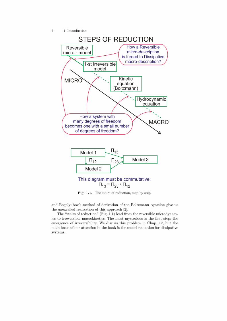
Fig. 1.1. The stairs of reduction, step by step.

and Bogolyubov’s method of derivation of the Boltzmann equation give usthe unexcelled realization of this approach [2].

The “stairs of reduction” (Fig. 1.1) lead from the reversible microdynam-ics to irreversible macrokinetics. The most mysterious is the first step: theemergence of irreversibility. We discuss this problem in Chap. 12, but themain focus of our attention in the book is the model reduction for dissipativesystems.

1.1 Ideas and references 3

U T xx J ( x ) P J ( x ) = ( 1 P ) J ( x ) x + k e r P

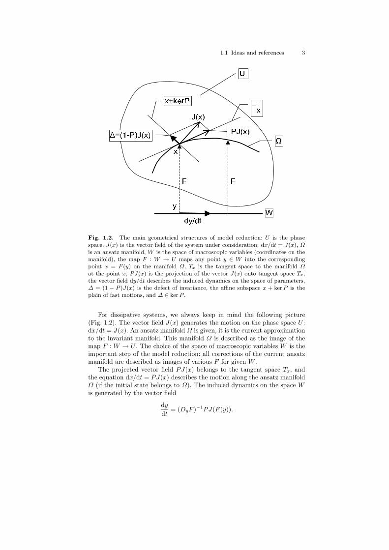
y WF Fd y / d tFig. 1.2. The main geometrical structures of model reduction: U is the phasespace, J(x) is the vector field of the system under consideration: dx/dt = J(x), Ωis an ansatz manifold, W is the space of macroscopic variables (coordinates on themanifold), the map F : W → U maps any point y ∈ W into the correspondingpoint x = F (y) on the manifold Ω, Tx is the tangent space to the manifold Ωat the point x, PJ(x) is the projection of the vector J(x) onto tangent space Tx,the vector field dy/dt describes the induced dynamics on the space of parameters,∆ = (1 − P )J(x) is the defect of invariance, the affine subspace x + ker P is theplain of fast motions, and ∆ ∈ ker P .

For dissipative systems, we always keep in mind the following picture(Fig. 1.2). The vector field J(x) generates the motion on the phase space U :dx/dt = J(x). An ansatz manifold Ω is given, it is the current approximationto the invariant manifold. This manifold Ω is described as the image of themap F : W → U . The choice of the space of macroscopic variables W is theimportant step of the model reduction: all corrections of the current ansatzmanifold are described as images of various F for given W .

The projected vector field PJ(x) belongs to the tangent space Tx, andthe equation dx/dt = PJ(x) describes the motion along the ansatz manifoldΩ (if the initial state belongs to Ω). The induced dynamics on the space Wis generated by the vector field

dy

dt= (DyF )−1PJ(F (y)).

4 1 Introduction

Here the inverse linear operator (DyF )−1 is defined on the tangent spaceTF (y), because the map F is assumed to be immersion, that is the differential(DyF ) is the isomorphism onto the tangent space TF (y).

The main focus of our analysis is the invariance equation1:

∆ = (1− P )J = 0,

the defect of invariance ∆ should vanish. It is a differential equation for anunknown map F : W → U . Solutions of this equation are invariant in thesense that the vector field J(x) is tangent to the manifold Ω = F (W ) foreach point x ∈ Ω. But this condition says nothing about the slowness of themanifold Ω.

How to choose the projector P? Another form of this question is: how todefine the plain of fast motions x + kerP? The choice of the projector P isambiguous, from the formal point of view, but the second law of thermody-namics gives a good hint [9]: the entropy should grow in the fast motion, andthe point x should be the point of entropy maximum on the plane of fastmotion x + kerP . That is, the subspace kerP should belong to the kernel ofthe entropy differential:

kerPx ⊂ kerDxS.

Of course, this rule is valid for closed systems with entropy, but it can be alsoextended onto open systems: the projection of the “thermodynamic part” ofJ(x) onto Tx should have the positive entropy production. If this thermo-dynamic requirement is valid for any ansatz manifold not tangent to theentropy levels and for any thermodynamic vector field, then the thermody-namic projector is unique [10]. Let us describe this projector P for given pointx, subspace Tx = imP, differential DxS of the entropy S at the point x andthe second differential of the entropy at the point x, the bilinear functional(D2

xS)x. We need the positively definite bilinear form 〈z|p〉x = −(D2xS)x(z, p)

(the entropic scalar product). There exists a unique vector g such that〈g|p〉x = DxS(p). It is the Riesz representation of the linear functional DxSwith respect to entropic scalar product. If g 6= 0 then the thermodynamicprojector is1 A.M. Lyapunov studied analytical solutions of similar equations near a fixed

point [3]. He found these solutions in a form of the Taylor series expansion andproved the convergency of those power series near the non-resonant fixed point(the Lyapunov auxiliary theorem). In 1960s the invariance equations approachwas developed, first of all, in the context of the Kolmogorov–Arnold–Moser the-ory for invariant tori computation [4–6], as a special analytical perturbationtheory [7,8]. Recently, the main task is to develop constructive non-perturbativemethods, because the series of perturbations theory diverge and, moreover, thehigh–order terms loose the physical sense for most interesting applications. Theseminal Kolmogorov’s idea was to use Newton’s method for solution of the invari-ance equation (instead of the Taylor series expansion) [4]. In this book we discussthe methods for invariant manifold construction that exploit the thermodynamicproperties of the kinetic equations.

1.1 Ideas and references 5

P (J) = P⊥(J) +g‖

〈g‖|g‖〉x〈g⊥|J〉x,

where P⊥ is the orthogonal projector onto Tx with respect the entropic scalarproduct, and the vector g is splitted onto tangent and orthogonal components:

g = g‖ + g⊥; g‖ = P⊥g; g⊥ = (1− P⊥)g.

This projector is defined if g‖ 6= 0.If g = 0 (the equilibrium point) then P (J) = P⊥(J).For given Tx, the thermodynamic projector (5.25) depends on the point

x through the x-dependence of the scalar product 〈|〉x, and also through thedifferential of S in x.

A dissipative system may have many closed positively invariant sets. Forexample, for every set of initial conditions K, union of all the trajectoriesx(t), t ≥ 0 with initial conditions x(0) ∈ K is positively invariant. Thus,the selection of the slow (stable) positively invariant manifolds becomes animportant problem2.

One of the difficulties in the problem of reducing the description is due tothe fact that there exists no commonly accepted formal definition of a slow(and stable) positively invariant manifold. This difficulty is resolved in Chap.4 of our book in the following way: First, we consider manifolds immersedinto a phase space and study their motion along trajectories. Second, we sub-tract from this motion the motion of immersed manifolds along themselves,and obtain a new equation for dynamics of manifolds in the phase space:the manifold Ω moves by the vector field ∆. It is the film extension of thedynamics:

dFt(y)dt

= ∆,

where the defect of invariance, ∆ = (1−P )J , depends on the point x = F (y)and on the tangent space to the manifold Ω = F (W ) at this point. Invariantmanifolds are fixed points for this extended dynamics, and slow invariantmanifolds are Lyapunov stable fixed points.

The main body of this book is about how to actually compute the slowinvariant manifold. We present three approaches to constructing slow (stable)positively invariant manifolds.

– Iteration method for solution of the invariance equation (Newton methodsubject to incomplete linearization);

2 Nevertheless, there exists a different point of view: “Non–uniqueness, when itarises, is irrelevant for modeling” [13], because the differences between the pos-sible manifolds are of the same order as the differences we set out to ignore inestablishing the low-dimensional model. We do not share this viewpoint becauseit may be relevant only if there exists a small parameter, and, moreover, onlyasymptotically when this small parameter tends to zero.

6 1 Introduction

– Relaxation methods based on the film extension of the original dynamicsystem;

– The method of natural projector that projects not the vector fields, butrather finite segments of trajectories.

The Newton method (with incomplete linearization) is the iterationmethod for solving the invariance equation. On each iteration we linearizethe invariance equation and solve obtained linear equation. In the defect ofinvariance ∆ = (1 − P )J(x) both the vector field J(x) = J(F (y)) (y ∈ W )and the projector P depend on the unknown map F (P depends on the pointx ∈ W and on the tangent space Tx = imDyF ). On each iteration we use forJ(F (y)) the first-order (linear in F ) approximation, and for P only the zero-order (constant) one. The iteration method with this incomplete linearizationleads to the slowest invariant manifold [11]. The Newton method (with in-complete linearization) is convenient for obtaining the explicit formulas –even one iteration can give a good approximation.

Relaxation methods are directed more towards the numerical implemen-tation. Nevertheless, several first steps also can give appropriate analyticalapproximations, competitive with other methods. These methods are basedon the stepwise solution of the differential equation dF (y)/dt = ∆ (the filmextension of the dynamics).

Finally, the natural projector method constructs not the manifold itselfbut a projection of slow dynamics onto some set of variables. This method isthe successor of two important methods: the Ehrenfests’ coarse-graining [15]and the Hilbert method for solution of the Boltzmann equation [16]. It canby applied to reversible and irreversible systems, and allows us to make thefirst step of reduction (see Fig. 1.1) as well as the following steps.

The Newton method subject to incomplete linearization was developedfor the construction of slow (stable) positively invariant manifolds in thefollowing problems:

– Derivation of the post–Navier–Stokes hydrodynamics from the Boltzmannequation [11,12,14,17].

– Description of the dynamics of polymers solutions [12,107].– Correction of the moment equations [12,21].– Reduced description for chemical kinetics [12,22,23,106].

Relaxation methods based on the film extension of the original dynamicsystem were applied to the Fokker–Planck equation [12, 24]. Applications ofthese methods in the theory of the Boltzmann equation can benefit from theestimations, obtained in the papers [26,27].

The method of natural projector was originally applied to derivation of thedissipative equations of macroscopic dynamics from the conservative equa-tions of the microscopic dynamics [12,30–36]. Using this method, new equa-tions were obtained for the post–Navier–Stokes hydrodynamics, equations of

1.1 Ideas and references 7

plasma hydrodynamics and others [31, 35]. This short-memory approxima-tion was applied to the Wigner formulation of quantum mechanics [37–39].The dissipative dynamics of a single quantum particle in a confining externalpotential is shown to take the form of a damped oscillator whose effectivefrequency and damping coefficients depend on the shape of the quantum-mechanical potential [36]. Further examples of the coarse-graining quantumfields dynamics can be found in [40]. The natural projector method can alsobe applied effectively to dissipative systems: instead of the Chapman–Enskogmethod in theory of the Boltzmann equation, for example.

The most natural initial approximation for the methods under considera-tion is a quasiequilibrium manifold. It is the manifold of conditional maximaof the entropy. The majority of works on nonequilibrium thermodynamicsdeal with corrections to quasi-equilibrium approximations, or with applica-tions of these approximations (with or without corrections). The constructionof the quasi-equilibrium allows for the following generalization: almost everymanifold can be represented as a set of minimizers of the entropy under lin-ear constraints. However, in contrast to the standard quasiequilibrium, theselinear constraints will depend on the point on the manifold. We describe thequasiequilibrium manifold and the quasiequilibrium projector on the tan-gent space of this manifold. This projector is orthogonal with respect to theentropic scalar product (the bilinear form defined by the negative second dif-ferential of the entropy). We construct the thermodynamical projector, whichtransforms the arbitrary vector field equipped with the given Lyapunov func-tion (the entropy) into a vector field with the same Lyapunov function for anarbitrary anzatz manifold which is not tangent to the level of the Lyapunovfunction. The uniqueness of this construction is demonstrated.

Here, a comment on the status of most of the statements in this bookis in order. Just like the absolute majority of claims concerning such thingsas general solutions of the Navier–Stokes or the Boltzmann equation, theyhave the status of being plausible. They can become theorems only if onerestricts essentially the set of the objects under consideration. Among suchrestrictions we should mention cases of the exact reduction, for example, exactderivation of hydrodynamics from kinetics [41, 43]. In these (still infinite-dimensional) examples one can compare different methods, for example, theNewton method with the methods of series summation in the perturbationtheory [43,44].

Also, it is necessary to stress here, that even if in the limit all the methodslead to the same results, they can give rather different approximations “onthe way”.

The rigorous foundation of the constructive methods of invariant mani-folds should, in particular, include theorems about persistence of invariantmanifolds under perturbations. For instance, the compact normally hyperbolicinvariant manifolds persist under small perturbations for finite-dimensionaldynamical systems [47, 48]. The most well-known result of this type is the

8 1 Introduction

Kolmogorov–Arnold–Moser theory about persistence of almost all invarianttori of completely integrable system under small perturbations [4–6].

Such theorems exist for some classes of infinite dimensional dissipativesystems too [49]. Unfortunately, it is not proven until now that many impor-tant systems (the Boltzmann equation, the three-dimensional Navier–Stokesequations, the Grad equations, etc.) belong to these classes. So, it is necessaryto act with these systems without a rigorous basis.

The new quantum field theory formulation of the problem of persistence ofinvariant tori in perturbed completely integrable systems was obtained [69],and a new proof of the KAM theorem for analytic Hamiltonians based onthe renormalization group method was given.

Two approaches to the construction of the invariant manifolds are widelyused: the Taylor series expansion for the solution of the invariance equa-tion [3, 51–53] and the method of renormalization group [54, 55, 57–60]. Theadvantages and disadvantages of the Taylor series expansion are well-known:constructivity versus the absence of physical meaning for the high-order terms(often), and divergence in the most interesting cases (often).

In the paper [57], a geometrical formulation of the renormalization groupmethod for global analysis was given. It was shown that the renormalizationgroup equation can be interpreted as an envelope equation. Recently [58] therenormalization group method was formulated in terms of invariant mani-folds. This method was applied to derive kinetic and transport equations fromthe respective microscopic equations [59]. The derived equations include theBoltzmann equation in classical mechanics (see also the paper [56], where itwas shown for the first time that kinetic equations such as the Boltzmannequation can be understood naturally as renormalization group equations),the Fokker–Planck equation, a rate equation in a quantum field theoreticalmodel.

From the point of view of the authors of the paper [56], the relation ofrenormalization group theory and reductive perturbation theory has simul-taneously been recognized: renormalization group equations are actually theslow-motion equations which are usually obtained by reductive perturbationmethods.

The renormalization group approach was applied to the stochastic Navier–Stokes equation in order to model fully developed fluid turbulence [61–63].For the evaluation of the relevant degrees of freedom the renormalizationgroup technique was revised for discrete systems in the recent paper [60].

The kinetic theory approach to subgrid modeling of fluid turbulence be-came more popular recently. [64–67]. A mean-field approach (filtering outsubgrid scales) was applied to the Boltzmann equation in order to derive asubgrid turbulence model based on kinetic theory. It was demonstrated [67]that the only Smagorinsky type model which survives in the hydrodynamiclimit on the viscosity time scale is the so-called tensor-diffusivity model [68].

1.1 Ideas and references 9

The first systematic and successful method of constructing invariant man-ifolds for dissipative systems was the celebrated Chapman-Enskog method [71]for the Boltzmann kinetic equation. The Chapman–Enskog method resultsin a series development of the so-called normal solution (the notion intro-duced by Hilbert [16]) where the one-body distribution function depends ontime and space only through its locally conserved moments. To the first ap-proximation, the Chapman–Enskog method leads to hydrodynamic equationswith transport coefficients expressed in terms of molecular scattering cross-sections. However, the higher order terms of the Chapman–Enskog expansionbring in the “ultra-violet catastrophe” (noticed first by Bobylev [73]) andnegative viscosity. This drawback pertinent to the Taylor series expansiondisappears as soon as the Newton method is used to construct the invariantmanifold [11].

The Chapman–Enskog method was generalized many times [77] and gaverise to a host of subsequent works and methods, such as the famous methodof the quasi-steady state in chemical kinetics, pioneered by Bodenstein andSemenov and explored in considerable detail by many authors (see, for ex-ample, [22, 78–82]), and the theory of singularly perturbed differential equa-tions [78,83–88].

There exists a set of methods to construct an ansatz for the invariantmanifold based on the spectral decomposition of the Jacobian. The idea touse the spectral decomposition of Jacobian fields in the problem of separatingthe motions into fast and slow originates from analysis of stiff systems [89],and from methods of sensitivity analysis in control theory [90, 91]. One ofthe currently most popular methods based on the spectral decomposition ofJacobian fields is the construction of the so-called intrinsic low-dimensionalmanifold (ILDM) [94].

These methods were thoroughly analyzed in two papers [95, 96]. It wasshown that the successive applications of the Computational Singular Per-turbation (CSP) algorithm (developed in [91]) generate, order by order, theasymptotic expansion of a slow manifold, and the manifold identified by theILDM technique (developed in [94]) agrees with the invariant manifold tosome order. An explicit algorithm based on the CSP method is designed forthe integration of stiff systems of PDEs by means of explicit schemes [92].The CSP analysis of time scales and manifolds in a transient flame-vortexinteraction was presented in [93].

The theory of inertial manifold is based on the special linear dominance inhigher dimensions. Let an infinite-dimensional system have a form: u+Au =R(u), where A is self-adjoint, and has a discrete spectrum λi → ∞ withsufficiently big gaps between λi, and let R(u) be continuous. One can buildthe slow manifold as the graph over a root space of A [97]. The textbook [101]provides an exhaustive introduction to the main ideas and methods of thistheory. Systems with linear dominance have limited utility in kinetics. Oftenthere are no big spectral gaps between λi, and even the sequence λi → ∞

10 1 Introduction

might be bounded (for example, this is the case for the model Bhatnagar–Gross–Krook (BGK) equations, or for the Grad equations). Nevertheless, theconcept of the inertial attracting manifold has wider field of applications thanthe theory, based on the linear dominance assumption.

The Newton method with incomplete linearization and the relaxationmethod allow us to find an approximate slow invariant manifolds withoutJacobian field spectral decomposition. Moreover, a necessary slow invariantsubspace of the Jacobian at the equilibrium point appears as a by-productof the Newton iterations (with incomplete linearization), or of the relaxationmethod.

It is of importance to search for minimal (or subminimal) sets of naturalparameters that uniquely determine the long-time behaviour of a system. Thisproblem was first discussed by Foias and Prodi [98] and by Ladyzhenskaya [99]for the two-dimensional Navier–Stokes equations. They have proved that thelong-time behaviour of solutions is completely determined by the dynamicsof sufficiently large number of Fourier modes. A general approach to theproblem on the existence of a finite number of determining parameters hasbeen discussed [100,101].

The past decade has witnessed a rapid development of the so-called setoriented numerical methods [102]. The purpose of these methods is to com-pute attractors, invariant manifolds (often, computation of stable and un-stable manifolds in hyperbolic systems [103–105]). Also, one of the centraltasks of these methods is to gain statistical information, i. e. computationsof physically observable invariant measures. The distinguished feature of themodern set-oriented methods of numerical dynamics is the use of ensemblesof trajectories within a relatively short propagation time instead of a longtime single trajectory.

In this book we systematically consider a discrete analog of the slow (sta-ble) positively invariant manifolds for dissipative systems, invariant grids.These invariant grids were introduced in [22]. Here we shall describe the New-ton method subject to incomplete linearization and the relaxation methodsfor the invariant grids [106].

It is worth mentioning that the problem of the grid correction is fullydecomposed into the tasks of the grid’s nodes correction. The edges betweenthe nodes appear only in the calculation of the tangent spaces at the nodes.This fact determines the high computational efficiency of the invariant gridsmethod.

Let the (approximate) slow invariant manifold for a dissipative system befound. Why have we constructed it? One important part of the answer to thisquestion is: We have constructed it to create models of open system dynamicsin the neighborhood of this manifold. Different approaches for this modelingare described.

We apply these methods to the problem of reduced description in poly-mer dynamics and derive the universal limit in dynamics of dilute polymeric

1.1 Ideas and references 11

solutions. It is represented by the revised Oldroyd 8 constants constitutiveequation [107] for the polymeric stress tensor. Coefficients of this constitu-tive equation are expressed in terms of the microscopic parameters. Thislimit of dynamics of dilute polymeric solutions is universal, and any phys-ically consistent equation should contain the obtained equation as a limit,or one should explain why it is not achieved. Such universal limit equationsare well-known in various fields of physics. For example, the Navier–Stokesequation in fluid dynamics is an universal limit for dynamics of simple gasdescribed by the Boltzmann equation, the Korteweg–De-Vries equation isuniversal in the description of the dispersive dissipative nonlinear waves, etc.

The phenomenon of invariant manifold explosion in driven open systemsis demonstrated on the example of dumbbell models of dilute polymeric so-lutions [110]. This explosion gives us a possible mechanism of drag reductionin dilute polymeric solutions [111].

Suppose that for the kinetic system the approximate invariant manifoldhas been constructed and the slow motion equations have been derived. Sup-pose that we have solved the slow motion system and obtained xsl(t). Weconsider the following two questions:

– How well does this solution approximate the true solution x(t) given thesame initial conditions?

– How is it possible to use the solution xsl(t) for its refinement withoutsolving the slow motion system (or its modifications) again?

These two questions are interconnected. The first question states the prob-lem of the accuracy estimation. The second one states the problem of post-processing [348–351]. We propose various algorithms for post-processing andaccuracy estimation, and give an example of application.

Our collection of methods and algorithms can be incorporated into re-cently developed technologies of computer-aided multiscale analysis whichenable “level jumping” between microscopic and macroscopic (system) lev-els. It is possible both for the traditional technique based on transition frommicroscopic equations to macroscopic equations and for the “equation-free”approach [108]. This approach developed in recent work [109], when success-ful, can bypass the derivation of the macroscopic evolution equations whenthese equations conceptually exist but are not available in closed form. Themathematics-assisted development of a computational superstructure mayenable alternative descriptions of the problem physics (e.g. Lattice Boltz-mann (LB), kinetic Monte- Carlo (KMC) or Molecular Dynamics (MD) mi-croscopic simulators, executed over relatively short time and space scales) toperform systems level tasks (integration over relatively large time and spacescales, coarse bifurcation analysis, optimization, and control) directly. It ispossible to use macroscopic invariant manifolds in this environment withoutexplicit equations.

12 1 Introduction

3 15

4 9 10 13

7 5 6

11

8

12

142

Fig. 1.3. Logical connections between chapters. All the chapters depend on Chap.3. For understanding examples and problems it may be useful (but not alwaysnecessary) to read Chap. 2.

1.2 Content and reading approaches

The present book comprises sections of two kinds. The first includes the sec-tions that contain basic notions, methods and algorithms. Another group ofsections entitled “Examples” contain various case studies where the meth-ods are applied to specific equations. Exposition in the “Examples” sectionsis not as consequent as in the basic sections. Most of the examples can beread more or less independently. Logical connections between chapters arepresented in Fig. 1.3.

The main results and notions presented in the book are as follows. In thisChap. 1 we present the main ideas, references, abstracts of chapters, and thepossible reading plans.

Chap. 2 is the second introduction, it introduces the main equations ofkinetics: the Boltzmann equation, equations of chemical kinetics, and theFokker–Planck equation. The main methods of reduction for these equa-tions are also discussed: from the Chapman–Enskog and Hilbert methodsto quasiequilibrium and quasi-steady state approximations.

In Chap. 3 we write down the invariance equation in the differential form.This equation gives the necessary conditions of invariance of a manifold im-mersed into the phase space of a dynamical system. In order to estimatethe discrepancy of an ansatz manifold, the defect of invariance if defined.

1.2 Content and reading approaches 13

The introduction of this defect of invariance requires a projector field. Thesenotions, defect of invariance and projector field, as well as the invarianceequation play the central role in the whole book.

Chap. 4 is devoted to the definition of slowness of a positively invariantmanifold. The equation of motion of the manifold (the “film”) immersed intothe phase space of the dynamical system is discussed (equation for the filmmotion). A slow positively invariant manifold is defined as a stable fixed pointfor this motion. The projector field introduced in Chap. 3 is crucial for thedefinition of the stability.

The main thermodynamic structures, the entropy, the entropic scalarproduct, quasiequilibrium, and the thermodynamic projector, are introducedin Chap. 5. The quasiequilibrium manifold is the manifold of conditionalentropy maxima for given values of macroscopic variables. These valuesparametrize this manifold. Most of the works on nonequilibrium thermo-dynamics deal with corrections to quasiequilibrium approximations, or withapplications of these approximations (with or without corrections). This view-point is not the only possible, but it proves very efficient for the constructionof a variety of useful models, approximations and equations, as well as meth-ods to solve them.

The entropic scalar product is generated by the second differential of theentropy. It endows the space of states by the unique distinguished Riemannianstructure. The thermodynamic projector is the operator which transformsthe arbitrary vector field equipped with the given Lyapunov function into avector field with the same Lyapunov function. Uniqueness of such projectoris proved.

In Chap. 5 we start the series of examples for the Boltzmann equations.First, we analyze the defect of invariance for the Local Maxwellian manifold:the manifold of the locally equilibrium distributions. Second, we present thequasi-equilibrium closure hierarchies for the Boltzmann equation. In 1949,Harold Grad [202] extended the basic assumption behind the Hilbert andChapman–Enskog methods (the space and time dependence of the normalsolutions is mediated by the five hydrodynamic moments). A physical ratio-nale behind the Grad moment method is an assumption of the decompositionof motion. (i) During the time of order τ , a set of distinguished moments M ′

(which include the hydrodynamic moments and a subset of higher-order mo-ment) does not change significantly as compared to the rest of the momentsM ′′ (the fast evolution). (ii) Towards the end of the fast evolution, the valuesof the moments M ′′ become unambiguously determined by the values of thedistinguished moments M ′. (iii) On the time of order θ À τ , dynamics ofthe distribution function is determined by the dynamics of the distinguishedmoments while the rest of the moments remains to be determined by thedistinguished moments (the slow evolution period).

An important generalization of the Grad moment method is the conceptof quasiequilibrium approximations. The quasiequilibrium distribution func-

14 1 Introduction

tion for a set of distinguished moments M ′ maximizes the entropy density Sfor fixed M ′. The quasiequilibrium manifold is the collection of the quasiequi-librium distribution functions for all admissible values of M . The quasiequi-librium approximation is the simplest and very useful (not only in the kinetictheory itself) implementation of the hypothesis about time separation.

The quasiequilibrium approximation does not exist if the highest ordermoment is an odd polynomial of velocity (therefore, there exists no quasiequi-librium for thirteen Grad’s moments). The Grad moment approximation isthe first-order expansion of the quasiequilibrium around the local Maxwellian.An explicit method of constructing of approximations (the Triangle EntropyMethod) is developed for strongly nonequilibrium problems of Boltzmann–type kinetics, i.e. when standard moment variables are insufficient. Thismethod enables one to treat any complicated nonlinear functionals that fitthe physics of a problem (such as, for example, rates of processes) as newindependent variables.

The method is applied to the problem of derivation of hydrodynamicsfrom the Boltzmann equation. New macroscopic variables are introduced(moments of the Boltzmann collision integral, or collision moments). Theyare treated as independent variables rather than as infinite moment series.This approach gives the complete account of the rates of scattering processes.Transport equations for scattering rates are obtained (the second hydrody-namic chain), similar to the usual moment chain (the first hydrodynamicchain). Using the triangle entropy method, three different types of macro-scopic description are considered. The first type involves only moments of dis-tribution functions, and the results coincide with those of the Grad method inthe Maximum Entropy version. The second type of description involves onlycollision moments. Finally, the third type involves both the moments andthe collision moments (the mixed description). The second and the mixedhydrodynamics are sensitive to the choice of the collision model. The sec-ond hydrodynamics is equivalent to the first hydrodynamics only for Maxwellmolecules, and the mixed hydrodynamics exists for all types of collision mod-els excluding Maxwell molecules. Various examples of the closure of the first,of the second, and of the mixed hydrodynamic chains are considered for thehard spheres model. It is shown, in particular, that the complete account ofscattering processes leads to a renormalization of transport coefficients.

We apply the developed method to a classical problem: determination ofmolecular dimensions (as diameters of equivalent hard spheres) from experi-mental viscosity data. It is the third example in Chap. 5.

The first non-perturbative method for solution of the invariance equationis developed in Chap. 6. It is the Newton method with incomplete lineariza-tion. The incomplete linearization means that in the Newton–type iterationfor the invariance equation we do not use the whole differential of the right-hand side of the invariance equation: the differential of the projector fieldis excluded. This modification of the Newton method leads to selection of

1.2 Content and reading approaches 15

the slowest invariant manifold. The series of examples for the Boltzmannequations is continued in this chapter. The non-perturbative correction tothe Local Maxwellian manifold is constructed, and the equations of the high-order (the post–Navier–Stokes) hydrodynamics are obtained.

In Chap. 5 we use the second law of thermodynamics – existence of theentropy – in order to equip the problem of constructing slow invariant man-ifolds with a geometric structure. The requirement of the entropy growth(universally, for all the reduced models) significantly restricts the form of thethermodynamic projectors. In Chap. 7 we introduce a different but equallyimportant argument – the micro-reversibility (T -invariance), and its macro-scopic consequences, the Onsager reciprocity relations. The main idea in thischapter is to use the reciprocity relations for the fast motions. In order to ap-preciate this idea, we should mention that the decomposition of motions intofast and slow is not unique. Requirement of the Onsager reciprocity relationsfor any equilibrium point of fast motions implies the selection (filtration) ofthe fast motions. We term this the Onsager filter. Equilibrium points of fastmotions are all the points on manifolds of slow motions. The formalism ofthe quasi-chemical representation is one of the most developed means of mod-elling, it makes it possible to “assemble” complex processes out of elementaryprocesses. This formalism is very natural for representation of the reciprocityrelations. And again, the Example to this chapter continues the “Boltzmannseries”. It is the quasi-chemical representation and the self-adjoint (i.e. On-sager) linearization of the Boltzmann collision operator in the slow, but notobligatory equilibrium states.

In Chap. 8 a new class of exactly solvable problems in nonequilibriumstatistical physics is described. The systems that allow the exact solution ofthe reduction problem are presented. Up to now, the problem of the exactrelationship between kinetics and hydrodynamics remains unsolved. All themethods used to establish this relationship are not rigorous, and involve ap-proximations. In this chapter, we consider situations where hydrodynamics isthe exact consequence of kinetics, and in that respect, a new class of exactlysolvable models of statistical physics has been established. The Chapman–Enskog method is treated as the Taylor series expansion approach to solvingthe appropriate invariance equation. A detailed treatment of the classicalChapman–Enskog derivation of hydrodynamics is given in the framework ofGrad’s moment equations. Grad’s systems are considered as the minimal ki-netic models where the Chapman–Enskog method can be studied exactly,thereby providing the basis to compare various approximations in extend-ing the hydrodynamic description beyond the Navier–Stokes approximation.Various techniques, such as the method of partial summation, the Pade ap-proximants, and the invariance principle are compared both in linear andnonlinear situations.

In Chap. 9 the “large stepping” relaxation method for solution of theinvariance equation is developed. The relaxation method is an alternative to

16 1 Introduction

the Newton iteration method described in Chap. 6: The initial approximationto the invariant manifold is moved with the film extension of the dynamicsdescribed in Chap. 4. The proposed step in time for the stepwise solutionof the film extension equation is the maximal possible step that does notviolate the thermodynamic conditions. In the examples, the idea of the largestepping is applied to the Fokker–Planck equation and to the initial layerproblem for the Boltzmann equation. The obtained approximate solutions ofthe initial layer problem are compared to the exact solutions.

How can we represent invariant manifolds numerically? How can we usethe numerical representation in all the methods for invariant manifold re-finement? Chapter 10 is devoted to answering these questions. A grid-basedversion of the method of invariant manifold is developed. The most essentialelement of this chapter is the systematic consideration of a discrete analogueof the slow (stable) positively invariant manifolds for dissipative systems, in-variant grids. The invariant grid is defined as a mapping of finite-dimensionalgrids into the phase space of a dynamic system. We define the differential op-erators on the grid as difference operators, hence, it is possible to definethe tangent space at each point of the grid mapped into the phase space. Ifthe tangent space is constructed, then the invariance equation can be writ-ten down. We describe the Newton method and the relaxation method forsolution of this discrete analogue of the invariance equation. Examples forthis chapter are taken from the chemical kinetics. One attractive feature oftwo-dimensional invariant grids is the possibility to use them as a screen, onwhich one can display different functions and dynamic of the system.

P. and T. Ehrenfest suggested in 1911 a model of dynamics with a coarse-graining of the original conservative system in order to introduce irreversibil-ity [15]. The Ehrenfests considered a partition of the phase space into smallcells, and they have suggested combining the motions of the phase space en-semble due to the Liouville equation with coarse-graining “shaking” steps –averaging of the density of the ensemble over the phase cells. This general-izes to the following: combination of the motion of the phase ensemble dueto microscopic equations with returns to the quasiequilibrium manifold whilepreserving the values of the macroscopic variables. In Chap. 11 we develop themethod of natural projector, a formalism of nonequilibrium thermodynamicsbased on this generalization.

The method of natural projector can be considered as a development ofthe ideas of the Hilbert method from the theory of the Boltzmann equation.The main new element in the method of natural projector with respect tothe Hilbert method is the construction of the macroscopic equations from themicroscopic equations, not just a “normal solution” to a microscopic equation.The obtained macroscopic equations contain one unknown parameter, thetime between coarse-graining (shaking) steps (τ). This parameter can beobtained from the experimental data, or from independent microscopic orphenomenological consideration.

1.2 Content and reading approaches 17

In the first example to this chapter the microscopic dynamics is givenby the one-particle Liouville equation. The set of macroscopic variables isdensity, momentum density, and the density of average kinetic energy. Thecorrespondent quasiequilibrium distribution is the local Maxwell distribu-tion. For the hydrodynamic equations, the zeroth (quasiequilibrium) approx-imation is given by the Euler equations of compressible nonviscous fluid.The next order approximation gives the Navier–Stokes equations which havedissipative terms. Higher-order approximations to the hydrodynamic equa-tions, when they are derived from the Boltzmann kinetic equation by theChapman–Enskog expansion (so-called Burnett approximation), are proneto various difficulties, in particular, they exhibit instability of sound waves atsufficiently short wave length (see Chap. 8). Here we demonstrate how modelhydrodynamic equations, including the post–Navier–Stokes approximations,can be derived on the basis of the coarse-graining idea, and find that theresulting equations are stable, contrary to the Burnett equation.

In the second example the fluctuation-dissipation formula is derived bythe method of natural projector and is illustrated by the explicit computationfor the exactly solvable McKean kinetic model [286]. It is demonstrated thatthe result is identical, on the one hand, to the sum of the Chapman–Enskogexpansion, and, on the other hand, to the exact solution of the invarianceequation.

In Chap. 12 the general geometrical framework of nonequilibrium ther-modynamics is developed. It is the generalization of the method of naturalprojector (Chap. 11) to large steps in time. The notion of macroscopicallydefinable ensembles is introduced. The thesis about macroscopically defin-able ensembles is suggested. This thesis should play the same role in thenonequilibrium thermodynamics, as the Church–Turing thesis in the theoryof computability. The primitive macroscopically definable ensembles are de-scribed. These are ensembles with macroscopically prepared initial states.

The method for computing trajectories of primitive macroscopically de-finable nonequilibrium ensembles is elaborated. These trajectories are repre-sented as sequences of deformed equilibrium ensembles and simple quadraticmodels between them. The primitive macroscopically definable ensemblesform a manifold in the space of ensembles. We call this manifold the film ofnonequilibrium states. The equation for the film and the equation for the en-semble motion on the film are written down. The notion of the invariant filmof non-equilibrium states, and the method of its approximate constructiontransform the problem of nonequilibrium kinetics into a series of problems ofequilibrium statistical physics. The developed methods allow us to solve theproblem of macro-kinetics even when there are no autonomous equations ofmacro-kinetics.

The slow invariant manifold for a closed system has been found. Whatnext? Chapter 13 gives the answer to this question. The theory of invari-ant manifolds is developed for weakly open systems. In the first example the

18 1 Introduction

method of invariant manifold for driven systems is developed for a derivationof a reduced description in kinetic equations of dilute polymeric solutions.The method applies to any models of polymers and is consistent with basicphysical requirements: frame invariance and dissipativity of resulting consti-tutive equation. It is demonstrated that this reduced description becomesuniversal in the limit of small Deborah and Weissenberg numbers, and it isrepresented by the revised Oldroyd 8 constants constitutive equation for thepolymeric stress tensor. This equation differs from the classical Oldroyd 8constants constitutive equation by one additional term. Coefficients of thisconstitutive equation are expressed in terms of the microscopic parametersof the polymer model. A systematic procedure of corrections to the revisedOldroyd 8 constants equations is developed. Results are tested with simpleflows.

In the second example in this chapter the derivation of macroscopic equa-tions from the simplest dumbbell models is revisited. It is demonstrated thatthe onset of the macroscopic description is sensitive to the flows. For theFENE-P model it is shown that there is a possibility of “explosion” of theGaussian manifold: with a small initial deviation, solution of the kinetic equa-tion very quickly deviate from the manifold, and then slowly come back to thestationary point located on the Gaussian manifold. Nevertheless, the Gaus-sian manifold remains invariant. Some consequences of these observationsare discussed. A new class of closures is introduced, the kinetic multipeakpolyhedra. Distributions of this type are expected in kinetic models withmultidimensional instability as universally, as the Gaussian distribution ap-pears for stable systems. The number of possible relatively stable states ofa nonequilibrium system grows as 2m, and the number of macroscopic pa-rameters is of the order mn, where n is the dimension of configuration space,and m is the number of independent unstable directions in this space. Theelaborated class of closures and equations pretends to describe the effects ofso-called “molecular individualism”.

How can we prove that all the attractors of a infinite-dimensional systembelong to a finite-dimensional manifold? How can we estimate the dimensionof this manifold? There are two methods for such estimations, discussed inChap. 14. First, if we find that k-dimensional volumes are contracted dueto dynamics, then (after some additional technical steps concerning exis-tence of the positively–invariant bounded set and uniformity of the volumecontraction on this set) we can state that the Hausdorff dimension of themaximal attractor is less, then k. Second, if we find the representation ofour system as a nonlinear kinetic system with conservation of supports ofdistributions, then (again, after some additional technical steps) we can statethat the asymptotics is finite-dimensional. This conservation of support hasa quasi-biological interpretation, the inheritance (if a gene is not presentedin an isolated population without mutations, then it cannot appear in time).

1.2 Content and reading approaches 19

The finite-dimensional asymptotics demonstrates the effects of “natural” se-lection.

The post-processing (Chap. 15) is a very simple, but attractive idea. Inthe method of invariant manifold we improve the whole manifold on eachiteration. If we need only one or several solutions, this whole manifold maybe too big for our goals, and we can restrict our activity by refinement of agiven solution: a curve instead of a multi-dimensional manifold. The classicalPicard iteration for a solution of a differential equation gives the simplestpost-processing. Various forms of post-processing are presented. In the ex-ample to this chapter the method which recognizes the onset and breakdownof the macroscopic description in microscopic simulations is presented. Themethod is based on the invariance of the macroscopic dynamics relative to themicroscopic dynamics, and it is demonstrated for a model of dilute polymericsolutions where it decides switching between Direct Brownian Dynamics sim-ulations and integration of constitutive equations.

The list of cited literature is by no means complete although we spenteffort in order to reflect at least the main directions of studies related tocomputations of the invariant manifolds. We think that this list is more orless exhaustive in the second-order approximation.

There are many different roads of reading this book. Chapter 3 is neces-sary for reading all of the other chapters, as is shown in the flowchart (Fig.1.3). Here we propose several possible roads. This is not the exhaustive list,and everybody can invent his own road.

The short formal road: Chap. 3, Sects.: 4.1, 5.1–5.3, 6.1, 7.1, 9.1, 10.1, 11.1,13.1–13.4, 15.1. If you are ready to look at the formal ordinary differentialequation dx

dt = J(x), x ∈ U, and to imagine in this form all the kineticequations, from the Boltzmann equation to the Fokker–Planck equation, thenthis formal road is the best way to start. After that, you can choose variousexamples and chapters. Before reading the examples sections, it may be usefulto look through Chap. 2.

The long formal road: Chaps. 3, 4, Sects.: 5.1–5.3, 6.1, 7.1, 9.1, 10.1, 11.1,13.1–13.4, 14.1, 14.2, 15.1.

The short Boltzmann road: Chap. 2 (including chemical kinetics), Chap.3, Sects. 5.1–5.3, 5.5, 6.1–6.3, Chap. 8. This road gives the invariance equa-tion, the Newton method with incomplete linearization for solution of thisequation, the theory of Local Maxwellian manifold, and the application ofthis method to correction of these manifolds. Chapter 8 adds the exact so-lutions of the reduction problem and the test of the developed methods onthese solutions.

The long Boltzmann road: Chap. 2 (including chemical kinetics), Chap.3, Sects. 5.1–5.3, 5.5, 5.6, 5.7, Chaps. 6–8, Sections 4.1, 9.1, 9.3. Exhaustivereading: everything concerning the Boltzmann equation.

20 1 Introduction

The nonequilibrium thermodynamic road: Chap. 2, Chap. 3, Sects. 4.1,5.1–5.4, 7.1, 9.1, Chaps. 11, 12, 14. This road can be naturally supplementedby some sections from the Boltzmann roads.

The short Grad road: Chaps. 2, 3, Sects. 5.1–5.6, 6.1, Chap. 8.