introductiontocommunicationsystems - university of … · number of institutions only teach digital...

Introduction to Communication Systems

Upamanyu Madhow

University of California, Santa Barbara

August 18, 2013

Contents

Preface 9

Acknowledgements 13

1 Introduction 15

1.1 Analog or Digital? . . . . . . . . . . . . . . . . . . . . . . . . . . . . . . . . . . . 15

1.1.1 Analog communication . . . . . . . . . . . . . . . . . . . . . . . . . . . . . 16

1.1.2 Digital communication . . . . . . . . . . . . . . . . . . . . . . . . . . . . . 16

1.1.3 Why digital? . . . . . . . . . . . . . . . . . . . . . . . . . . . . . . . . . . 20

1.2 A Technology Perspective . . . . . . . . . . . . . . . . . . . . . . . . . . . . . . . 21

1.3 Scope of this Textbook . . . . . . . . . . . . . . . . . . . . . . . . . . . . . . . . . 24

1.4 Concept Inventory . . . . . . . . . . . . . . . . . . . . . . . . . . . . . . . . . . . 24

1.5 Endnotes . . . . . . . . . . . . . . . . . . . . . . . . . . . . . . . . . . . . . . . . . 25

2 Signals and Systems 27

2.1 Complex Numbers . . . . . . . . . . . . . . . . . . . . . . . . . . . . . . . . . . . 28

2.2 Signals . . . . . . . . . . . . . . . . . . . . . . . . . . . . . . . . . . . . . . . . . . 30

2.3 Linear Time Invariant Systems . . . . . . . . . . . . . . . . . . . . . . . . . . . . 36

2.3.1 Discrete time convolution . . . . . . . . . . . . . . . . . . . . . . . . . . . 43

2.3.2 Multi-rate systems . . . . . . . . . . . . . . . . . . . . . . . . . . . . . . . 45

2.4 Fourier Series . . . . . . . . . . . . . . . . . . . . . . . . . . . . . . . . . . . . . . 46

2.4.1 Fourier Series Properties and Applications . . . . . . . . . . . . . . . . . . 49

2.5 Fourier Transform . . . . . . . . . . . . . . . . . . . . . . . . . . . . . . . . . . . . 51

2.5.1 Fourier Transform Properties . . . . . . . . . . . . . . . . . . . . . . . . . 53

2.5.2 Numerical computation using DFT . . . . . . . . . . . . . . . . . . . . . . 57

2.6 Energy Spectral Density and Bandwidth . . . . . . . . . . . . . . . . . . . . . . . 59

2.7 Baseband and Passband Signals . . . . . . . . . . . . . . . . . . . . . . . . . . . . 61

2.8 The Structure of a Passband Signal . . . . . . . . . . . . . . . . . . . . . . . . . . 63

2.8.1 Time Domain Relationships . . . . . . . . . . . . . . . . . . . . . . . . . . 63

2.8.2 Frequency Domain Relationships . . . . . . . . . . . . . . . . . . . . . . . 70

2.8.3 Complex baseband equivalent of passband filtering . . . . . . . . . . . . . 74

3

2.8.4 General Comments on Complex Baseband . . . . . . . . . . . . . . . . . . 75

2.9 Wireless Channel Modeling in Complex Baseband . . . . . . . . . . . . . . . . . . 77


2.11 Endnotes . . . . . . . . . . . . . . . . . . . . . . . . . . . . . . . . . . . . . . . . . 79

3 Analog Communication Techniques 87

3.1 Terminology and notation . . . . . . . . . . . . . . . . . . . . . . . . . . . . . . . 88

3.2 Amplitude Modulation . . . . . . . . . . . . . . . . . . . . . . . . . . . . . . . . . 89

3.2.1 Double Sideband (DSB) Suppressed Carrier (SC) . . . . . . . . . . . . . . 89

3.2.2 Conventional AM . . . . . . . . . . . . . . . . . . . . . . . . . . . . . . . . 92

3.2.3 Single Sideband Modulation (SSB) . . . . . . . . . . . . . . . . . . . . . . 98

3.2.4 Vestigial Sideband (VSB) Modulation . . . . . . . . . . . . . . . . . . . . . 103

3.2.5 Quadrature Amplitude Modulation . . . . . . . . . . . . . . . . . . . . . . 105

3.2.6 Concept synthesis for AM . . . . . . . . . . . . . . . . . . . . . . . . . . . 106

3.3 Angle Modulation . . . . . . . . . . . . . . . . . . . . . . . . . . . . . . . . . . . . 107

3.3.1 Limiter-Discriminator Demodulation . . . . . . . . . . . . . . . . . . . . . 110

3.3.2 FM Spectrum . . . . . . . . . . . . . . . . . . . . . . . . . . . . . . . . . . 111

3.3.3 Concept synthesis for FM . . . . . . . . . . . . . . . . . . . . . . . . . . . 114

3.4 The Superheterodyne Receiver . . . . . . . . . . . . . . . . . . . . . . . . . . . . . 115

3.5 The Phase Locked Loop . . . . . . . . . . . . . . . . . . . . . . . . . . . . . . . . 118

3.5.1 PLL Applications . . . . . . . . . . . . . . . . . . . . . . . . . . . . . . . . 121

3.5.2 Mathematical Model for the PLL . . . . . . . . . . . . . . . . . . . . . . . 122

3.5.3 PLL Analysis . . . . . . . . . . . . . . . . . . . . . . . . . . . . . . . . . . 123

3.6 Some Analog Communication Systems . . . . . . . . . . . . . . . . . . . . . . . . 128

3.6.1 FM radio . . . . . . . . . . . . . . . . . . . . . . . . . . . . . . . . . . . . 128

3.6.2 Analog broadcast TV . . . . . . . . . . . . . . . . . . . . . . . . . . . . . . 129

3.7 Problems . . . . . . . . . . . . . . . . . . . . . . . . . . . . . . . . . . . . . . . . . 131

4 Digital Modulation 141

4.1 Signal Constellations . . . . . . . . . . . . . . . . . . . . . . . . . . . . . . . . . . 142

4.2 Bandwidth Occupancy . . . . . . . . . . . . . . . . . . . . . . . . . . . . . . . . . 145

4.2.1 Power Spectral Density . . . . . . . . . . . . . . . . . . . . . . . . . . . . . 145

4.2.2 PSD of a linearly modulated signal . . . . . . . . . . . . . . . . . . . . . . 147

4.3 Design for Bandlimited Channels . . . . . . . . . . . . . . . . . . . . . . . . . . . 150

4.3.1 Nyquist’s Sampling Theorem and the Sinc Pulse . . . . . . . . . . . . . . . 150

4.3.2 Nyquist Criterion for ISI Avoidance . . . . . . . . . . . . . . . . . . . . . . 153

4.3.3 Bandwidth efficiency . . . . . . . . . . . . . . . . . . . . . . . . . . . . . . 155

4.3.4 Power-bandwidth tradeoffs: a sneak preview . . . . . . . . . . . . . . . . . 157

4.3.5 The Nyquist criterion at the link level . . . . . . . . . . . . . . . . . . . . 159

4

4.3.6 Linear modulation as a building block . . . . . . . . . . . . . . . . . . . . 160

4.4 Orthogonal and Biorthogonal Modulation . . . . . . . . . . . . . . . . . . . . . . . 160

4.5 Proofs of the Nyquist theorems . . . . . . . . . . . . . . . . . . . . . . . . . . . . 164


4.7 Endnotes . . . . . . . . . . . . . . . . . . . . . . . . . . . . . . . . . . . . . . . . . 167

4.A Power spectral density of a linearly modulated signal . . . . . . . . . . . . . . . . 178

4.B Simulation resource: bandlimited pulses and upsampling . . . . . . . . . . . . . . 180

5 Probability and Random Processes 185

5.1 Probability Basics . . . . . . . . . . . . . . . . . . . . . . . . . . . . . . . . . . . . 185

5.2 Random Variables . . . . . . . . . . . . . . . . . . . . . . . . . . . . . . . . . . . . 191

5.3 Multiple Random Variables, or Random Vectors . . . . . . . . . . . . . . . . . . . 196

5.4 Functions of random variables . . . . . . . . . . . . . . . . . . . . . . . . . . . . . 202

5.5 Expectation . . . . . . . . . . . . . . . . . . . . . . . . . . . . . . . . . . . . . . . 206

5.5.1 Expectation for random vectors . . . . . . . . . . . . . . . . . . . . . . . . 210

5.6 Gaussian Random Variables . . . . . . . . . . . . . . . . . . . . . . . . . . . . . . 211

5.6.1 Joint Gaussianity . . . . . . . . . . . . . . . . . . . . . . . . . . . . . . . . 216

5.7 Random Processes . . . . . . . . . . . . . . . . . . . . . . . . . . . . . . . . . . . 224

5.7.1 Running example: sinusoid with random amplitude and phase . . . . . . . 224

5.7.2 Basic definitions . . . . . . . . . . . . . . . . . . . . . . . . . . . . . . . . . 225

5.7.3 Second order statistics . . . . . . . . . . . . . . . . . . . . . . . . . . . . . 227

5.7.4 Wide Sense Stationarity and Stationarity . . . . . . . . . . . . . . . . . . . 228

5.7.5 Power Spectral Density . . . . . . . . . . . . . . . . . . . . . . . . . . . . . 229

5.7.6 Gaussian random processes . . . . . . . . . . . . . . . . . . . . . . . . . . 234

5.8 Noise Modeling . . . . . . . . . . . . . . . . . . . . . . . . . . . . . . . . . . . . . 235

5.9 Linear Operations on Random Processes . . . . . . . . . . . . . . . . . . . . . . . 240

5.9.1 Filtering . . . . . . . . . . . . . . . . . . . . . . . . . . . . . . . . . . . . . 240

5.9.2 Correlation . . . . . . . . . . . . . . . . . . . . . . . . . . . . . . . . . . . 243


5.11 Endnotes . . . . . . . . . . . . . . . . . . . . . . . . . . . . . . . . . . . . . . . . . 247

5.12 Problems . . . . . . . . . . . . . . . . . . . . . . . . . . . . . . . . . . . . . . . . . 247

5.A Q function bounds and asymptotics . . . . . . . . . . . . . . . . . . . . . . . . . . 260

5.B Approximations using Limit Theorems . . . . . . . . . . . . . . . . . . . . . . . . 260

5.C Noise Mechanisms . . . . . . . . . . . . . . . . . . . . . . . . . . . . . . . . . . . . 262

5.D The structure of passband random processes . . . . . . . . . . . . . . . . . . . . . 263

5.D.1 Baseband representation of passband white noise . . . . . . . . . . . . . . 265

5.E SNR Computations for Analog Modulation . . . . . . . . . . . . . . . . . . . . . . 266

5.E.1 Noise Model and SNR Benchmark . . . . . . . . . . . . . . . . . . . . . . . 266

5.E.2 SNR for Amplitude Modulation . . . . . . . . . . . . . . . . . . . . . . . . 266

5

5.E.3 SNR for Angle Modulation . . . . . . . . . . . . . . . . . . . . . . . . . . . 269

6 Optimal Demodulation 277

6.1 Hypothesis Testing . . . . . . . . . . . . . . . . . . . . . . . . . . . . . . . . . . . 278

6.1.1 Error probabilities . . . . . . . . . . . . . . . . . . . . . . . . . . . . . . . 279

6.1.2 ML and MAP decision rules . . . . . . . . . . . . . . . . . . . . . . . . . . 280

6.1.3 Soft Decisions . . . . . . . . . . . . . . . . . . . . . . . . . . . . . . . . . . 285

6.2 Signal Space Concepts . . . . . . . . . . . . . . . . . . . . . . . . . . . . . . . . . 287

6.2.1 Representing signals as vectors . . . . . . . . . . . . . . . . . . . . . . . . 288

6.2.2 Modeling WGN in signal space . . . . . . . . . . . . . . . . . . . . . . . . 292

6.2.3 Hypothesis testing in signal space . . . . . . . . . . . . . . . . . . . . . . . 293

6.2.4 Optimal Reception in AWGN . . . . . . . . . . . . . . . . . . . . . . . . . 295

6.2.5 Geometry of the ML decision rule . . . . . . . . . . . . . . . . . . . . . . . 298

6.3 Performance Analysis of ML Reception . . . . . . . . . . . . . . . . . . . . . . . . 301

6.3.1 The Geometry of Errors . . . . . . . . . . . . . . . . . . . . . . . . . . . . 301

6.3.2 Performance with binary signaling . . . . . . . . . . . . . . . . . . . . . . . 302

6.3.3 M-ary signaling: scale-invariance and SNR . . . . . . . . . . . . . . . . . . 305

6.3.4 Performance analysis for M-ary signaling . . . . . . . . . . . . . . . . . . . 310

6.3.5 Performance analysis for M-ary orthogonal modulation . . . . . . . . . . . 318

6.4 Bit Error Probability . . . . . . . . . . . . . . . . . . . . . . . . . . . . . . . . . . 320

6.5 Link Budget Analysis . . . . . . . . . . . . . . . . . . . . . . . . . . . . . . . . . . 322


6.7 Endnotes . . . . . . . . . . . . . . . . . . . . . . . . . . . . . . . . . . . . . . . . . 329

6.A Irrelevance of component orthogonal to signal space . . . . . . . . . . . . . . . . . 347

7 Channel Coding 349

7.1 Motivation . . . . . . . . . . . . . . . . . . . . . . . . . . . . . . . . . . . . . . . . 350

7.2 Model for Channel Coding . . . . . . . . . . . . . . . . . . . . . . . . . . . . . . . 352

7.3 Shannon’s Promise . . . . . . . . . . . . . . . . . . . . . . . . . . . . . . . . . . . 354

7.3.1 Design Implications of Shannon Limits . . . . . . . . . . . . . . . . . . . . 360

7.4 Introducing linear codes . . . . . . . . . . . . . . . . . . . . . . . . . . . . . . . . 361

7.5 Soft decisions and belief propagation . . . . . . . . . . . . . . . . . . . . . . . . . 370

7.6 Concept inventory on channel coding . . . . . . . . . . . . . . . . . . . . . . . . . 374

7.7 Endnotes . . . . . . . . . . . . . . . . . . . . . . . . . . . . . . . . . . . . . . . . . 376

7.8 Problems . . . . . . . . . . . . . . . . . . . . . . . . . . . . . . . . . . . . . . . . . 376

8 Dispersive Channels and MIMO 387

8.1 Singlecarrier System Model . . . . . . . . . . . . . . . . . . . . . . . . . . . . . . 388

8.1.1 Signal Model . . . . . . . . . . . . . . . . . . . . . . . . . . . . . . . . . . 388

6

8.1.2 Noise Model and SNR . . . . . . . . . . . . . . . . . . . . . . . . . . . . . 393

8.2 Linear equalization . . . . . . . . . . . . . . . . . . . . . . . . . . . . . . . . . . . 394

8.2.1 Adaptive MMSE Equalization . . . . . . . . . . . . . . . . . . . . . . . . . 397

8.2.2 Geometric Interpretation and Analytical Computations . . . . . . . . . . . 400

8.3 Orthogonal Frequency Division Multiplexing . . . . . . . . . . . . . . . . . . . . . 406

8.3.1 DSP-centric implementation . . . . . . . . . . . . . . . . . . . . . . . . . . 408

8.4 MIMO . . . . . . . . . . . . . . . . . . . . . . . . . . . . . . . . . . . . . . . . . . 413

8.4.1 The linear array . . . . . . . . . . . . . . . . . . . . . . . . . . . . . . . . . 413

8.4.2 Beamsteering . . . . . . . . . . . . . . . . . . . . . . . . . . . . . . . . . . 415

8.4.3 Rich Scattering and MIMO-OFDM . . . . . . . . . . . . . . . . . . . . . . 418

8.4.4 Diversity . . . . . . . . . . . . . . . . . . . . . . . . . . . . . . . . . . . . . 421

8.4.5 Spatial multiplexing . . . . . . . . . . . . . . . . . . . . . . . . . . . . . . 426


8.6 Endnotes . . . . . . . . . . . . . . . . . . . . . . . . . . . . . . . . . . . . . . . . . 430

8.7 Problems . . . . . . . . . . . . . . . . . . . . . . . . . . . . . . . . . . . . . . . . . 431

Epilogue 445

7

Preface

Progress in telecommunications over the past two decades has been nothing short of revolution-ary, with communications taken for granted in modern society to the same extent as electricity.There is therefore a persistent need for engineers who are well-versed in the principles of commu-nication systems. These principles apply to communication between points in space, as well ascommunication between points in time (i.e, storage). Digital systems are fast replacing analogsystems in both domains. This book has been written in response to the following core question:what is the basic material that an undergraduate student with an interest in communicationsshould learn, in order to be well prepared for either industry or graduate school? For example, anumber of institutions only teach digital communication, assuming that analog communicationis dead or dying. Is that the right approach? From a purely pedagogical viewpoint, there arecritical questions related to mathematical preparation: how much mathematics must a studentlearn to become well-versed in system design, what should be assumed as background, and atwhat point should the mathematics that is not in the background be introduced? Classically,students learn probability and random processes, and then tackle communication. This does notquite work today: students increasingly (and I believe, rightly) question the applicability of thematerial they learn, and are less interested in abstraction for its own sake. On the other hand,I have found from my own teaching experience that students get truly excited about abstractconcepts when they discover their power in applications, and it is possible to provide the meansfor such discovery using software packages such as Matlab. Thus, we have the opportunity toget a new generation of students excited about this field: by covering abstractions “just in time”to shed light on engineering design, and by reinforcing concepts immediately using software ex-periments in addition to conventional pen-and-paper problem solving, we can remove the lagbetween learning and application, and ensure that the concepts stick.

This textbook represents my attempt to act upon the preceding observations, and is an out-growth of my lectures for a two-course undergraduate elective sequence on communication atUCSB, which is often also taken by some beginning graduate students. Thus, it can be used asthe basis for a two course sequence in communication systems, or a single course on digital com-munication, at the undergraduate or beginning graduate level. The book also provides a reviewor introduction to communication systems for practitioners, easing the path to study of moreadvanced graduate texts and the research literature. The prerequisite is a course on signals andsystems, together with an introductory course on probability. The required material on randomprocesses is included in the text.

A student who masters the material here should be well-prepared for either graduate schoolor the telecommunications industry. The student should leave with an understanding of base-band and passband signals and channels, modulation formats appropriate for these channels,random processes and noise, a systematic framework for optimum demodulation based on signalspace concepts, performance analysis and power-bandwidth tradeoffs for common modulationschemes, introduction to communication techniques over dispersive channels, and a hint of thepower of information theory and channel coding. Given the significant ongoing research anddevelopment activity in wireless communication, and the fact that an understanding of wirelesslink design provides a sound background for approaching other communication links, materialenabling hands-on discovery of key concepts for wireless system design is interspersed throughout

9

the textbook.

The goal of the lecture-style exposition in this book is to clearly articulate a selection of conceptsthat I deem fundamental to communication system design, rather than to provide comprehensivecoverage. “Just in time” coverage is provided by organizing and limiting the material so that weget to core concepts and applications as quickly as possible, and by sometimes asking the readerto operate with partial information (which is, of course, standard operating procedure in the realworld of engineering design).

Organization

• Chapter 1 provides a perspective on communication systems, including a discussion of thetransition from analog to digital communication and how it colors the selection of material inthis text. Chapter 2 provides a review of signals and systems (biased towards communicationsapplications), and then discusses the complex baseband representation of passband signals andsystems, emphasizing its critical role in modeling, design and implementation. A software labon modeling and undoing phase offsets in complex baseband, while providing a sneak preview ofdigital modulation, is included.

• Chapter 2 also includes a section on wireless channel modeling in complex baseband using raytracing, reinforced by a software lab which applies these ideas to simulate link time variationsfor a lamppost based broadband wireless network.

• Chapter 3 covers analog communication techniques which are relevant even as the world goesdigital, including superheterodyne reception and phase locked loops. Legacy analog modulationtechniques are discussed to illustrate core concepts, as well as in recognition of the fact thatsuboptimal analog techniques such as envelope detection and limiter-discriminator detectionmay have to be resurrected as we push the limits of digital communication in terms of speed andpower consumption.

• Chapter 4 discusses digital modulation, including linear modulation using constellations suchas Pulse Amplitude Modulation (PAM), Quadrature Amplitude Modulation (QAM), and PhaseShift Keying (PSK), and orthogonal modulation and its variants. The chapter includes discussionof the number of degrees of freedom available on a bandlimited channel, the Nyquist criterionfor avoidance of intersymbol interference, and typical choices of Nyquist and square root Nyquistsignaling pulses. We also provide a sneak preview of power-bandwidth tradeoffs (with detaileddiscussion postponed until the effect of noise has been modeled in Chapters 5 and 6). A softwarelab providing a hands-on feel for Nyquist signaling is included in this chapter.

The material in Chapters 2 through 4 requires only a background in signals and systems.

• Chapter 5 provides a review of basic probability and random variables, and then introducesrandom processes. This chapter provides detailed discussion of Gaussian random variables, vec-tors and processes; this is essential for modeling noise in communication systems. Exampleswhich provide a preview of receiver operations in communication systems, and computation ofperformance measures such as error probability and signal-to-noise ratio (SNR), are provided.Discussion of circular symmetry of white noise, and noise analysis of analog modulation tech-niques is placed in an appendix, since this is material that is often skipped in modern courses oncommunication systems.

• Chapter 6 covers classical material on optimum demodulation for M-ary signaling in the pres-ence of additive white Gaussian noise (AWGN). The background on Gaussian random variables,vectors and processes developed in Chapter 5 is applied to derive optimal receivers, and to analyzetheir performance. After discussing error probability computation as a function of SNR, we areable to combine the materials in Chapters 4 and 6 for a detailed discussion of power-bandwidthtradeoffs. Chapter 6 concludes with an introduction to link budget analysis, which provides

10

guidelines on the choice of physical link parameters such as transmit and receive antenna gains,and distance between transmitter and receiver, using what we know about the dependence oferror probability as a function of SNR. This chapter includes a software lab which builds on theNyquist signaling lab in Chapter 4 by investigating the effect of noise. It also includes anothersoftware lab simulating performance over a time-varying wireless channel, examining the effectsof fading and diversity, and introduces the concept of differential demodulation for avoidance ofexplicit channel tracking.

Chapters 2 through 6 provide a systematic lecture-style exposition of what I consider core con-cepts in communication at an undergraduate level.

• Chapter 7 provides a glimpse of information theory and coding whose goal is to stimulate thereader to explore further using more advanced resources such as graduate courses and textbooks.It shows the critical role of channel coding, provides an initial exposure to information-theoreticperformance benchmarks, and discusses belief propagation in detail, reinforcing the basic con-cepts through a software lab.

• Chapter 8 provides a first exposure to the more advanced topics of communication over dis-persive channels, and of multiple antenna systems, often termed space-time communication, orMultiple Input Multiple Output (MIMO) communication. These topics are grouped together be-cause they use similar signal processing tools. We emphasize lab-style “discovery” in this chapterusing three software labs, one on adaptive linear equalization for singlecarrier modulation, one onbasic OFDM transceiver operations, and one on MIMO signal processing for space-time codingand spatial multiplexing. The goal is for students to acquire hands-on insight that hopefullymotivates them to undertake a deeper and more systematic investigation.

• Finally, the epilogue contains speculation on future directions in communications research andtechnology. The goal is to provide a high-level perspective on where mastery of the introductorymaterial in this textbook could lead, and to argue that the innovations that this field has alreadyseen set the stage for many exciting developments to come.

The role of software: Software problems and labs are integrated into the text, while “code frag-ments” implementing core functionalities provided in the text. While code can be providedonline, separate from the text (and indeed, sample code is made available online for instruc-tors), code fragments are integrated into the text for two reasons. First, they enable readers toimmediately see the software realization of a key concept as they read the text. Second, I feelthat students would learn more by putting in the work of writing their own code, building onthese code fragments if they wish, rather than using code that is easily available online. Theparticular software that we use is Matlab, because of its widespread availability, and because ofits importance in design and performance evaluation in both academia and industry. However,the code fragments can also be viewed as “pseudocode,” and can be easily implemented usingother software packages or languages. Block-based packages such as Simulink (which builds uponMatlab) are avoided here, because the use of software here is pedagogical rather than aimed at,say, designing a complete system by putting together subsystems as one might do in industry.

Suggestions for using this book

I view Chapter 2 (complex baseband), Chapter 4 (digital modulation), and Chapter 6 (optimumdemodulation) as core material that must be studied to understand the concepts underlyingmodern communication systems. Chapter 6 relies on the probability and random processesmaterial in Chapter 5, especially the material on jointly Gaussian random variables and WGN,but the remaining material in Chapter 5 can be covered selectively, depending on the students’background. Chapter 3 (analog communication techniques) is designed such that it can becompletely skipped if one wishes to focus solely on digital communication. Finally, Chapter

11

7 and Chapter 8 contain glimpses of advanced material that can be sampled according to theinstructor’s discretion. The qualitative discussion in the epilogue is meant to provide the studentwith perspective, and is not intended for formal coverage in the classroom.

In my own teaching at UCSB, this material forms the basis for a two-course sequence, withChapters 2-4 covered in the first course, and Chapters 5-6 covered in the second course, with thedispersive channels portion of Chapter 8 providing the basis for the labs in the second course.The content of these courses are constantly being revised, and it is anticipated that the materialon channel coding and MIMO may displace some of the existing material in the future. UCSB ison a quarter system, hence the coverage is fast-paced, and many topics are omitted or skimmed.There is ample material here for a two-semester undergraduate course sequence. For a singleone-semester course, one possible organization is to cover Chapter 4, a selection of Chapter 5,Chapter 6, and if time permits, Chapter 7.

12

Acknowledgements

This book grew out of lecture notes for an undergraduate elective course sequence in communi-cations at UCSB, and I am grateful to the succession of students who have used, and providedencouraging comments on, the evolution of the course sequence and the notes. I would also liketo acknowledge faculty in the communications area at UCSB who were kind enough to give mea “lock” on these courses over the past few years, as I was developing this textbook.

The first priority in a research university is to run a vibrant research program, hence I mustacknowledge the extraordinarily capable graduate students in my research group over the yearsthis textbook was developed. They have done superb research with minimal supervision fromme, and the strength of their peer interactions and collaborations is what gave me the mentalspace, and time, needed to write this textbook. Current and former group members who havedirectly helped with aspects of this book include Andrew Irish, Babak Mamandipoor, DineshRamasamy, Maryam Eslami Rasekh, Sumit Singh, Sriram Venkateswaran, and Aseem Wadhwa.

I gratefully acknowledge the funding agencies that have provided support for our research group inrecent years, including the National Science Foundation (NSF), the Army Research Office (ARO),the Defense Advanced Research Projects Agency (DARPA), and the Systems on Nanoscale In-formation Fabrics (SONIC), a center supported by DARPA and Microelectronics Advanced Re-search Corporation (MARCO). One of the primary advantages of a research university is thatundergraduate education is influenced, and kept up to date, by cutting edge research. This text-book embodies this paradigm both in its approach (an emphasis on what one can do with whatone learns) and content (emphasis of concepts that are fundamental background for research inthe area).

I thank Phil Meyler and his colleagues at Cambridge University Press for encouraging me to ini-tiate this project, and for their blend of patience and persistence in getting me to see it throughdespite a host of other commitments. I also thank the anonymous reviewers of the book pro-posal and sample chapters sent to Cambridge several years back for their encouragement andconstructive comments. I am also grateful to a number of faculty colleagues who have givenencouragement, helpful suggestions, and pointers to alternative pedagogical approaches: Pro-fessor Soura Dasgupta (University of Iowa), Professor Jerry Gibson (UCSB), Professor GerhardKramer (Technische Universitat Munchen, Munich, Germany), Professor Phil Schniter (OhioState University), and Professor Venu Veeravalli (University of Illinois at Urbana-Champaign).

Finally, I would like to thank my wife and children for always being the most enjoyable andinteresting people to spend time with. Recharging my batteries in their company, and that ofour many pets, is what provides me with the energy needed for an active professional life.

13

Chapter 1

Introduction

This textbook provides an introduction to the conceptual underpinnings of communication tech-nologies. Most of us directly experience such technologies daily: browsing (and audio/videostreaming from) the Internet, sending/receiving emails, watching television, or carrying out aphone conversation. Many of these experiences occur on mobile devices that we carry aroundwith us, so that we are always connected to the cyberworld of modern communication systems.In addition, there is a huge amount of machine-to-machine communication that we do not di-rectly experience, but which are indispensable for the operation of modern society. Examplesinclude signaling between routers on the Internet, or between processors and memories on anycomputing device.

We define communication as the process of information transfer across space or time. Commu-nication across space is something we have an intuitive understanding of: for example, radiowaves carry our phone conversation between our cell phone and the nearest base station, andcoaxial cables (or optical fiber, or radio waves from a satellite) deliver television from a remotelocation to our home. However, a moment’s thought shows that that communication across time,or storage of information, is also an everyday experience, given our use of storage media such ascompact discs (CDs), digital video discs (DVDs), hard drives and memory sticks. In all of theseinstances, the key steps in the operation of a communication link are as follows:(a) insertion of information into a signal, termed the transmitted signal, compatible with thephysical medium of interest.(b) propagation of the signal through the physical medium (termed the channel) in space ortime;(c) extraction of information from the signal (termed the received signal) obtained after propa-gation through the medium.In this book, we study the fundamentals of modeling and design for these steps.

Chapter Plan: In Section 1.1, we provide a high-level description of analog and digital com-munication systems, and discuss why digital communication is the inevitable design choice inmodern systems. In Section 1.2, we briefly provide a technological perspective on recent devel-opments in communication. We do not attempt to provide a comprehensive discussion of thefascinating history of communication: thanks to the advances in communication that brought usthe Internet, it is easy to look it up online! A discussion of the scope of this textbook is providedin Section 1.3.

1.1 Analog or Digital?

Even without defining information formally, we intuitively understand that speech, audio, andvideo signals contain information. We use the term message signals for such signals, since these

15

are the messages we wish to convey over a communication system. In their original form–both during generation and consumption–these message signals are analog: they are continuoustime signals, with the signal values also lying in a continuum. When someone plays the violin,an analog acoustic signal is generated (often translated to an analog electrical signal using amicrophone). Even when this music is recorded onto a digital storage medium such as a CD (usingthe digital communication framework outlined in Section 1.1.2), when we ultimately listen to theCD being played on an audio system, we hear an analog acoustic signal. The transmitted signalscorresponding to physical communication media are also analog. For example, in both wirelessand optical communication, we employ electromagnetic waves, which correspond to continuoustime electric and magnetic fields taking values in a continuum.

1.1.1 Analog communication

Message

InformationSource

Modulator Channel Demodulatorconsumer

Information

signalTransmitted Received

signalMessage

signal signal

Figure 1.1: Block diagram for an analog communication system. The modulator transformsthe message signal into the transmitted signal. The channel distorts and adds noise to thetransmitted signal. The demodulator extracts an estimate of the message signal from the receivedsignal arriving from the channel.

Given the analog nature of both the message signal and the communication medium, a naturaldesign choice is to map the analog message signal (e.g., an audio signal, translated from theacoustic to electrical domain using a microphone) to an analog transmitted signal (e.g., a radiowave carrying the audio signal) that is compatible with the physical medium over which we wishto communicate (e.g., broadcasting audio over the air from an FM radio station). This approachto communication system design, depicted in Figure 1.1, is termed analog communication. Earlycommunication systems were all analog: examples include AM (amplitude modulation) and FM(frequency modulation) radio, analog television, first generation cellular phone technology (basedon FM), vinyl records, audio cassettes, and VHS or beta videocassettes

While analog communication might seem like the most natural option, it is in fact obsolete. Cel-lular phone technologies from the second generation onwards are digital, vinyl records and audiocassettes have been supplanted by CDs, and videocassettes by DVDs. Broadcast technologiessuch as radio and television are often slower to upgrade because of economic and political factors,but digital broadcast radio and television technologies are either replacing or sidestepping (e.g.,via satellite) analog FM/AM radio and television broadcast. Let us now define what we mean bydigital communication, before discussing the reasons for the inexorable trend away from analogand towards digital communication.

1.1.2 Digital communication

The conceptual basis for digital communication was established in 1948 by Claude Shannon,when he founded the field of information theory. There are two main threads to this theory:• Source coding and compression: Any information-bearing signal can be represented ef-ficiently, to within a desired accuracy of reproduction, by a digital signal (i.e., a discrete timesignal taking values from a discrete set), which in its simplest form is just a sequence of binary

16

digits (zeros or ones), or bits. This is true whether the information source is text, speech, au-dio or video. Techniques for performing the mapping from the original source signal to a bitsequence are generically termed source coding. They often involve compression, or removal ofredundancy, in a manner that exploits the properties of the source signal (e.g., the heavy spatialcorrelation among adjacent pixels in an image can be exploited to represent it more efficientlythan a pixel-by-pixel representation).• Digital information transfer: Once the source encoding is done, our communication task re-duces to reliably transferring the bit sequence at the output of the source encoder across space ortime, without worrying about the original source and the sophisticated tricks that have been usedto encode it. The performance of any communication system depends on the relative strengthsof the signal and noise or interference, and the distortions imposed by the channel. Shannonshowed that, once we fix these operational parameters for any communication channel, thereexists a maximum possible rate of reliable communication, termed the channel capacity. Thus,given the information bits at the output of the source encoder, in principle, we can transmit themreliably over a given link as long as the information rate is smaller than the channel capacity,and we cannot transmit them reliably if the information rate is larger than the channel capac-ity. This sharp transition between reliable and unreliable communication differs fundamentallyfrom analog communication, where the quality of the reproduced source signal typically degradesgradually as the channel conditions get worse.

A block diagram for a typical digital communication system based on these two threads is shownin Figure 1.2. We now briefly describe the role of each component, together with simplifiedexamples of its function.

Decoder

Channelencoder

Modulator Channel DemodulatorChanneldecoder

Information

bitsbits

Information

Codedbits

Transmittedsignal signal

Received Estimatesof coded bits

Digitalcommunication

link

Information SourceEncoderSource

Informationbits

signalMessage

Source InformationConsumerbits

Information

signalMessage

Figure 1.2: Components of a digital communication system.

Source encoder: As already discussed, the source encoder converts the message signal into asequence of information bits. The information bit rate depends on the nature of the messagesignal (e.g., speech, audio, video) and the application requirements. Even when we fix the classof message signals, the choice of source encoder is heavily dependent on the setting. For example,video signals are heavily compressed when they are sent over a cellular link to a mobile device,but are lightly compressed when sent to an high definition television (HDTV) set. A cellular link

17

can support a much smaller bit rate than, say, the cable connecting a DVD player to an HDTVset, and a smaller mobile display device requires lower resolution than a large HDTV screen. Ingeneral, the source encoder must be chosen such that the bit rate it generates can be supportedby the digital communication link we wish to transfer information over. Other than this, sourcecoding can be decoupled entirely from link design (we comment further on this a bit later).Example: A laptop display may have resolution 1024× 768 pixels. For a grayscale digital image,the intensity for each pixel might be represented by 8 bits. Multiplying by the number ofpixels gives us about 6.3 million bits, or about 0.8 Mbyte (a byte equals 8 bits). However,for a typical image, the intensities for neighboring pixels are heavily correlated, which can beexploited for significantly reducing the number of bits required to represent the image, withoutnoticeably distorting it. For example, one could take a two-dimensional Fourier transform, whichconcentrates most of the information in the image at lower frequencies and then discard manyof the high frequency coefficients. There are other possible transforms one could use, and alsoseveral more processing stages, but the bottomline is that, for natural images, state of the artimage compression algorithms can provide 10X compression (i.e., reduction in the number of bitsrelative to the original uncompressed digital image) with hardly any perceptual degradation. Farmore aggressive compression ratios are possible if we are willing to tolerate more distortion. Forvideo, in addition to the spatial correlation exploited for image compression, we can also exploittemporal correlation across successive frames.

Channel encoder: The channel encoder adds redundancy to the information bits obtainedfrom the source encoder, in order to facilitate error recovery after transmission over the channel.It might appear that we are putting in too much work, adding redundancy just after the sourceencoder has removed it. However, the redundancy added by the channel encoder is tailored tothe channel over which information transfer is to occur, whereas the redundancy in the originalmessage signal is beyond our control, so that it would be inefficient to keep it when we transmitthe signal over the channel.Example: The noise and distortion introduced by the channel can cause errors in the bits wesend over it. Consider the following abstraction for a channel: we can send a string of bits (zerosor ones) over it, and the channel randomly flips each bit with probability 0.01 (i.e., the channelhas a 1% error rate). If we cannot tolerate this error rate, we could repeat each bit that we wishto send three times, and use a majority rule to decide on its value. Now, we only make an errorif two or more of the three bits are flipped by the channel. It is left as an exercise to calculatethat an error now happens with probability approximately 0.0003 (i.e., the error rate has gonedown to 0.03%). That is, we have improved performance by introducing redundancy. Of course,there far more sophisticated and efficient techniques for introducing redundancy than the simplerepetition strategy just described; see Chapter 7.

Modulator: The modulator maps the coded bits at the output of the channel encoder to atransmitted signal to be sent over the channel. For example, we may insist that the transmittedsignal fit within a given frequency band and adhere to stringent power constraints in a wirelesssystem, where interference between users and between co-existing systems is a major concern.Unlicensed WiFi transmissions typically occupy 20-40 MHz of bandwidth in the 2.4 or 5 GHzbands. Transmissions in fourth generation cellular systems may often occupy bandwidths rangingfrom 1-20 MHz at frequencies ranging from 700 MHz to 3 GHz. While these signal bandwidthsare being increased in an effort to increase data rates (e.g., up to 160 GHz for emerging WiFistandards, and up to 100 MHz for emerging cellular standards), and new frequency bands arebeing actively explored (see the epilogue for more discussion), the transmitted signal still needsto be shaped to fit within certain spectral constraints.Example: Suppose that we send bit value 0 by transmitting the signal s(t), and bit value 1 bytransmitting −s(t). Even for this simple example, we must design the signal s(t) so it fits withinspectral constraints (e.g., two different users may use two different segments of spectrum to avoidinterfering with each other), and we must figure out how to prevent successive bits of the sameuser from interfering with each other. For wireless communication, these signals are voltages

18

generated by circuits coupled to antennas, and are ultimately emitted as electromagnetic wavesfrom the antennas.

The channel encoder and modulator are typically jointly designed, keeping in mind the antici-pated channel conditions, and the result is termed a coded modulator.

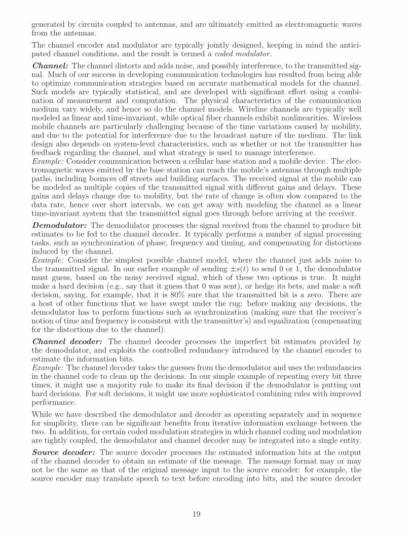
Channel: The channel distorts and adds noise, and possibly interference, to the transmitted sig-nal. Much of our success in developing communication technologies has resulted from being ableto optimize communication strategies based on accurate mathematical models for the channel.Such models are typically statistical, and are developed with significant effort using a combi-nation of measurement and computation. The physical characteristics of the communicationmedium vary widely, and hence so do the channel models. Wireline channels are typically wellmodeled as linear and time-invariant, while optical fiber channels exhibit nonlinearities. Wirelessmobile channels are particularly challenging because of the time variations caused by mobility,and due to the potential for interference due to the broadcast nature of the medium. The linkdesign also depends on system-level characteristics, such as whether or not the transmitter hasfeedback regarding the channel, and what strategy is used to manage interference.Example: Consider communication between a cellular base station and a mobile device. The elec-tromagnetic waves emitted by the base station can reach the mobile’s antennas through multiplepaths, including bounces off streets and building surfaces. The received signal at the mobile canbe modeled as multiple copies of the transmitted signal with different gains and delays. Thesegains and delays change due to mobility, but the rate of change is often slow compared to thedata rate, hence over short intervals, we can get away with modeling the channel as a lineartime-invariant system that the transmitted signal goes through before arriving at the receiver.

Demodulator: The demodulator processes the signal received from the channel to produce bitestimates to be fed to the channel decoder. It typically performs a number of signal processingtasks, such as synchronization of phase, frequency and timing, and compensating for distortionsinduced by the channel.Example: Consider the simplest possible channel model, where the channel just adds noise tothe transmitted signal. In our earlier example of sending ±s(t) to send 0 or 1, the demodulatormust guess, based on the noisy received signal, which of these two options is true. It mightmake a hard decision (e.g., say that it guess that 0 was sent), or hedge its bets, and make a softdecision, saying, for example, that it is 80% sure that the transmitted bit is a zero. There area host of other functions that we have swept under the rug: before making any decisions, thedemodulator has to perform functions such as synchronization (making sure that the receiver’snotion of time and frequency is consistent with the transmitter’s) and equalization (compensatingfor the distortions due to the channel).

Channel decoder: The channel decoder processes the imperfect bit estimates provided bythe demodulator, and exploits the controlled redundancy introduced by the channel encoder toestimate the information bits.Example: The channel decoder takes the guesses from the demodulator and uses the redundanciesin the channel code to clean up the decisions. In our simple example of repeating every bit threetimes, it might use a majority rule to make its final decision if the demodulator is putting outhard decisions. For soft decisions, it might use more sophisticated combining rules with improvedperformance.

While we have described the demodulator and decoder as operating separately and in sequencefor simplicity, there can be significant benefits from iterative information exchange between thetwo. In addition, for certain coded modulation strategies in which channel coding and modulationare tightly coupled, the demodulator and channel decoder may be integrated into a single entity.

Source decoder: The source decoder processes the estimated information bits at the outputof the channel decoder to obtain an estimate of the message. The message format may or maynot be the same as that of the original message input to the source encoder: for example, thesource encoder may translate speech to text before encoding into bits, and the source decoder

19

may output a text message to the end user.Example: For the example of a digital image considered earlier, the compressed image can betranslated back to a pixel-by-pixel representation by taking the inverse spatial Fourier transformof the coefficients that survived the compression.

We are now ready to compare analog and digital communication, and discuss why the trendtowards digital is inevitable.

1.1.3 Why digital?

Comparing the block diagrams for analog and digital communication in Figures 1.1 and 1.2,respectively, we see that the digital communication system involves far more processing. How-ever, this is not an obstacle for modern transceiver design, due to the exponential increase inthe computational power of low-cost silicon integrated circuits. Digital communication has thefollowing key advantages.

Optimality: For a point-to-point link, it is optimal to separately optimize source coding andchannel coding, as long we do not mind the delay and processing incurred in doing so. Dueto this source-channel separation principle, we can leverage the best available source codes andthe best available channel codes in designing a digital communication system, independentlyof each other. Efficient source encoders must be highly specialized. For example, state of theart speech encoders, video compression algorithms, or text compression algorithms are verydifferent from each other, and are each the result of significant effort over many years by a largecommunity of researchers. However, once source encoding is performed, the coded modulationscheme used over the communication link can be engineered to transmit the information bitsreliably, regardless of what kind of source they correspond to, with the bit rate limited onlyby the channel and transceiver characteristics. Thus, the design of a digital communicationlink is source-independent and channel-optimized. In contrast, the waveform transmitted in ananalog communication system depends on the message signal, which is beyond the control of thelink designer, hence we do not have the freedom to optimize link performance over all possiblecommunication schemes. This is not just a theoretical observation: in practice, huge performancegains are obtained from switching from analog to digital communication.

Scalability: While Figure 1.2 shows a single digital communication link between source en-coder and decoder, under the source-channel separation principle, there is nothing preventingus from inserting additional links, putting the source encoder and decoder at the end points.This is because digital communication allows ideal regeneration of the information bits, henceevery time we add a link, we can focus on communicating reliably over that particular link. (Ofcourse, information bits do not always get through reliably, hence we typically add error recoverymechanisms such as retransmission, at the level of an individual link or end-to-end.) Anotherconsequence of the source-channel separation principle is that, since information bits are trans-ported without interpretation, the same link can be used to carry multiple kinds of messages. Aparticularly useful approach is to chop the information bits up into discrete chunks, of packets,which can then be processed independently on each link. These properties of digital communica-tion are critical for enabling massively scalable, general purpose, communication networks suchas the Internet. Such networks can have large numbers of digital communication links, possiblywith different characteristics, independently engineered to provide bit pipes that can supportdata rates. Messages of various kinds, after source encoding, are reduced to packets, and thesepackets are switched along different paths along the network, depending on the identities of thesource and destination nodes, and the loads on different links in the network. None of this wouldbe possible with analog communication: link performance in an analog communication systemdepends on message properties, and successive links incur noise accumulation, which limits thenumber of links which can be cascaded.

20

The preceding makes it clear that source-channel separation is crucial in the formation and growthof modern communication networks. It is worth noting, however, that joint source-channel designcan provide better performance in some settings, especially when there are constraints on delayor complexity, or if multiple users are being supported simultaneously on a given communicationmedium. In practice, this means that “local” violations of the separation principle (e.g., over awireless last hop in a communication network) may be a useful design trick.

1.2 A Technology Perspective

We now discuss some technology trends and concepts that have driven the astonishing growthin communication systems in the past two decades, and that are expected to impact futuredevelopments in this area. Our discussion is structured in terms of big technology “stories.”

Technology story 1: The Internet. Some of the key ingredients that contributed to itsgrowth and the essential role it plays in our lives are as follows:• Any kind of message can be chopped up into packets and routed across the network, using anInternet Protocol (IP) that is simple to implement in software;• Advances in optical fiber communication and high-speed digital hardware enable a super-fast“core” of routers connected by very high-speed, long-range links, that enable world-wide coverage;• The World Wide Web, or web, makes it easy to organize information into interlinked hypertextdocuments which can be browsed from anywhere in the world;• The digitization of content (audio, video, books) means that ultimately “all” information isexpected to be available on the web;• Search engines enable us to efficiently search for this information;• Connectivity applications such as email, teleconferencing, videoconferencing and online socialnetworks have become indispensable in our daily lives.

Technology story 2: Wireless. Cellular mobile networks are everywhere, and are based onthe breakthrough concept that ubiquitous tetherless connectivity can be provided by breakingthe world into cells, with “spatial reuse” of precious spectrum resources in cells that are “farenough” apart. Base stations serve mobiles in their cells, and hand them off to adjacent basestations when the mobile moves to another cell. While cellular networks were invented to supportvoice calls for mobile users, today’s mobile devices (e.g., “smart phones” and tablet computers)are actually powerful computers with displays large enough for users to consume video on the go.Thus, cellular networks must now support seamless access to the Internet. The billions of mobiledevices in use easily outnumber desktop and laptop computers, so that the most important partsof the Internet today are arguably the cellular networks at its edge. Mobile service providers arehaving great difficulty keeping up with the increase in demand resulting from this convergenceof cellular and Internet; by some estimates, the capacity of cellular networks must be scaled upby several orders of magnitude, at least in densely populated urban areas! As discussed in theepilogue, a major challenge for the communication researcher and technologist, therefore, is tocome up with the breakthroughs required to deliver such capacity gains.

Another major success in wireless is WiFi, a catchy term for a class of standardized wirelesslocal area network (WLAN) technologies based on the IEEE 802.11 family of standards. Cur-rently, WiFi networks use unlicensed spectrum in the 2.4 and 5 GHz bands, and have come intowidespread use in both residential and commercial environments. WiFi transceivers are nowincorporated into almost every computer and mobile device. One way of alleviating the cellularcapacity crunch that was just mentioned is to offload Internet access to the nearest WiFi net-work. Of course, since different WiFi networks are often controlled by different entities, seamlessswitching between cellular and WiFi is not always possible.

It is instructive to devote some thought to the contrast between cellular and WiFi technologies.Cellular transceivers and networks are far more tightly engineered. They employ spectrum that

21

mobile operators pay a great deal of money to license, hence it is critical to use this spectrumefficiently. Furthermore, cellular networks must provide robust wide-area coverage in the face ofrapid mobility (e.g., automobiles at highway speeds). In contrast, WiFi uses unlicensed (i.e., free!)spectrum, must only provide local coverage, and typically handles much slower mobility (e.g.,pedestrian motion through a home or building). As a result, WiFi can be more loosely engineeredthan cellular. It is interesting to note that despite the deployment of many uncoordinatedWiFi networks in an unlicensed setting, WiFi typically provides acceptable performance, partlybecause the relatively large amount of unlicensed spectrum (especially in the 5 GHz band) allowsfor channel switching when encountering excessive interference, and partly because of naturallyoccurring spatial reuse (WiFi networks that are “far enough” do not interfere with each other).Of course, in densely populated urban environments with many independently deployed WiFinetworks, the performance can deteriorate significantly, a phenomenon sometimes referred to asa tragedy of the commons (individually selfish behavior leading to poor utilization of a sharedresource). As we briefly discuss in the epilogue, both the cellular and WiFi design paradigmsneed to evolve to meet our future needs.

Technology story 3: Moore’s law. Moore’s “law” is actually an empirical observation at-tributed to Gordon Moore, one of the co-founders of Intel Corporation. It can be paraphrased assaying that the density of transistors in an integrated circuit, and hence the amount of compu-tation per unit cost, can be expected to increase exponentially over time. This observation hasbecome a self-fulfilling prophecy, because it has been taken up by the semiconductor industryas a growth benchmark driving their technology roadmap. While Moore’s law may be slowingdown somewhat, it has already had a spectacular impact on the communications industry bydrastically lowering the cost and increasing the speed of digital computation. By convertinganalog signals to the digital domain as soon as possible, advanced transceiver algorithms canbe implemented in digital signal processing (DSP) using low-cost integrated circuits, so that re-search breakthroughs in coding and modulation can be quickly transitioned into products. Thisleads to economies of scale that have been critical to the growth of mass market products in bothwireless (e.g., cellular and WiFi) and wireline (e.g., cable modems and DSL) communication.

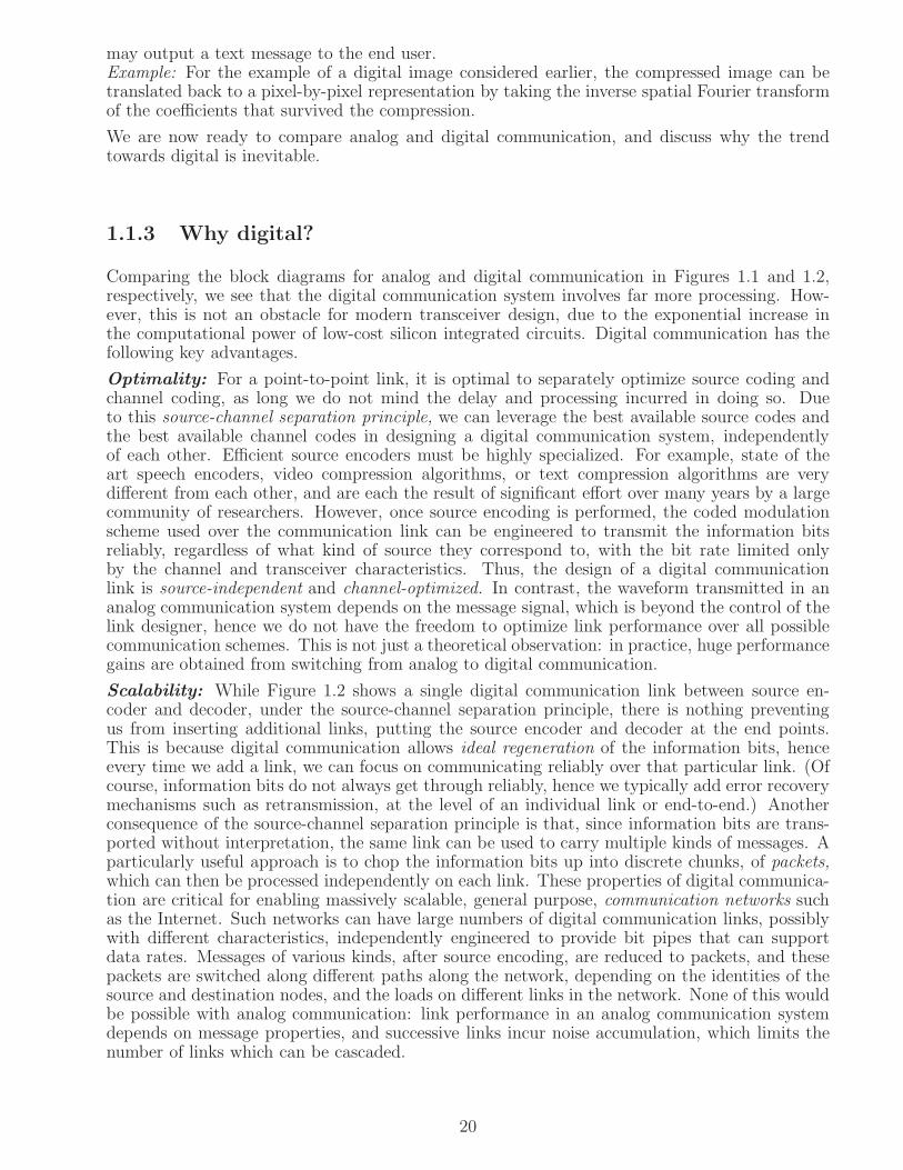
Figure 1.3: The Internet has a core of routers and servers connected by high-speed fiber links,with wireless networks hanging off the edge (figure courtesy Aseem Wadhwa).

How do these stories come together? The sketch in Figure 1.3 highlights key building blocksof the Internet today. The core of the network consists of powerful routers that direct packetsof data from an incoming edge to an outgoing edge, and servers (often housed in large datacenters) that serve up content requested by clients such as personal computers and mobile devices.The elements in the core network are connected by high-speed optical fiber. Wireless can beviewed as hanging off the edge of the Internet. Wide area cellular networks may have worldwidecoverage, but each base station is typically connected by a high-speed link to the wired Internet.

22

WiFi networks are wireless local area networks, typically deployed indoors (but potentially alsoproviding outdoor coverage for low-mobility scenarios) in homes and office buildings, connected tothe Internet via last mile links, which might run over copper wires (a legacy of wired telephony,with transceivers typically upgraded to support broadband Internet access) or coaxial cable(originally deployed to deliver cable television, but now also providing broadband Internet access).Some areas have been upgraded to optical fiber to the curb or even to the home, while someothers might be remote enough to require wireless last mile solutions.

Figure 1.4: A segment of a cellular network with idealized hexagonal shapes (figure courtesyAseem Wadhwa).

Zooming in now on cellular networks, Figure 1.4 shows three adjacent cells in a cellular networkwith hexagonal cells. A working definition of a cell is that it is the area around a base stationwhere the signal strength is higher than that from other base stations. Of course, under realisticpropagation conditions, cells are never hexagonal, but the concept of spatial reuse still holds: theinterference between distant cells can be neglected, hence they can use the same communicationresources. For example, in Figure 1.4, we might decide to use three different frequency bandsin the three cells shown, but might then reuse these bands in other cells. Figure 1.4 also showsthat a user may be simultaneously in range of multiple base stations when near cell boundaries.Crossing these boundaries may result in a handoff from one base station to another. In addition,near cell boundaries, a mobile device may be in communication with multiple base stationssimultaneously, a concept known as soft handoff.

It is useful for a communication system designer to be aware of the preceding “big picture” oftechnology trends and network architectures in order to understand how to direct his or hertalents as these systems continue to evolve (the epilogue contains more detailed speculationregarding this evolution). However, the first order of business is to acquire the fundamentalsrequired to get going in this field. These are quite simply stated: a communication systemdesigner must be comfortable with mathematical modeling (in order to understand the state ofthe art, as well as to devise new models as required), and with devising and evaluating signalprocessing algorithms based on these models. The goal of this textbook is to provide a firstexposure to such a technical background.

23

1.3 Scope of this Textbook

Referring to the block diagram of a digital communication system in Figure 1.2, our focus inthis textbook is to provide an introduction to design of a digital communication link as showninside the dashed box. While we are primarily interested in digital communication, circuit de-signers implementing such systems must deal with analog waveforms, hence we believe that arudimentary background in analog communication techniques, as provided in this book, is usefulfor the communication system designer. We do not discuss source encoding and decoding inthis book; these topics are highly specialized and technical, and doing them justice requires anentire textbook of its own at the graduate level. A detailed outline of the book is provided inthe preface, hence we restrict ourselves here to summarizing the roles of the various chapters:Chapter 2: introduces the signal processing background required for DSP-centric implementa-tions of communication transceivers;Chapter 3: provides just enough background on analog communication techniques (can beskipped if only focused on digital communication);Chapter 4: discusses digital modulation techniques;Chapter 5: provides the probability background required for receiver design, including noisemodeling;Chapter 6: discusses design and performance analysis of demodulators in digital communicationsystems for idealized link models;Chapter 7: provides an initial exposure to channel coding techniques and benchmarks;Chapter 8: provides an introduction to approaches for handling channel dispersion, and to mul-tiple antenna communication;Epilogue: discusses emerging trends shaping research and development in communications.

Chapters 2, 4 and 6 are core material that must be mastered (much of Chapter 5 is also corematerial, but some readers may already have enough probability background that they can skip,or skim, it). Chapter 3 is highly recommended for communication system designers with interestin radio frequency circuit design, since it highlights, at a high level, some of the ideas and issuesthat come up there. Chapters 7 and 8 are independent of each other, and contain more advancedmaterial that may not always fit within an undergraduate curriculum. They contain “hands-on”introductions to these topics via code fragments and software labs that hopefully encourage thereader to explore further.

1.4 Concept Inventory

The goal of this chapter is to provide an intellectual framework and motivation for the rest ofthis textbook. Some of the key concepts are as follows.

• Communication refers to information transfer across either space or time, where the latterrefers to storage media.• Signals carrying information and signals that can be sent over a communication medium areboth inherently analog (i.e., continuous-time, continuous-valued).• Analog communication corresponds to transforming an analog message waveform directly intoan analog transmitted waveform at the transmitter, and undoing this transformation at thereceiver.• Digital communication corresponds to first reducing message waveforms to information bits,and then transporting these bits over the communication channel.• Digital communication requires the following steps: source encoding and decoding, modulationand demodulation, channel encoding and decoding.• While digital communication requires more processing steps than analog communication, it hasthe advantages of optimality and scalability, hence there is an unstoppable trend from analog to

24

digital.• The growth in communication has been driven by major technology stories including theInternet, wireless and Moore’s law.• Key components of the communication system designer’s toolbox are mathematical modelingand signal processing.

1.5 Endnotes

There are a large number of textbooks on communication systems at both the undergraduate andgraduate level. Undergraduate texts include Haykin [1], Proakis and Salehi [2], Pursley [3], andZiemer and Tranter [4]. Graduate texts, which typically focus on digital communication includeBarry, Lee and Messerschmitt [5], Benedetto and Biglieri [6], Madhow [7], and Proakis and Salehi[8]. The first coherent exposition of the modern theory of communication receiver design is inthe classical (graduate level) textbook by Wozencraft and Jacobs [9]. Other important classicalgraduate level texts are Viterbi and Omura [10] and Blahut [11]. More specialized references (e.g.,on signal processing, information theory, channel coding, wireless communication) are mentionedin later chapters. In addition to these textbooks, an overview of many important topics can befound in the recently updated mobile communications handbook [12] edited by Gibson.

This book is intended to be accessible to readers who have never been exposed to communicationsystems before. It has some overlap with more advanced graduate texts (e.g., Chapters 2, 4, 5and 6 here overlap heavily with Chapters 2 and 3 in the author’s own graduate text [7]), andprovides the technical background and motivation required to easily access these more advancedtexts. Of course, the best way to continue building expertise in the field is by actually workingin it. Research and development in this field requires study of the research literature, of morespecialized texts (e.g., on information theory, channel coding, synchronization), and of commer-cial standards. The Institute for Electrical and Electronics Engineers (IEEE) is responsible forpublication of many conference proceedings and journals in communications: major conferencesinclude IEEE Global Telecommunications Conference (Globecom), IEEE International Com-munications Conference (ICC), major journals and magazines include IEEE CommunicationsMagazine, IEEE Transactions on Communications, IEEE Journal on Selected Areas in Commu-nications. Closely related fields such as information theory and signal processing have their ownconferences, journals and magazines. Major conferences include the IEEE International Sympo-sium on Information Theory (ISIT) and IEEE International Conference on Acoustics, Speech andSignal Processing (ICASSP), journals include the IEEE Transactions on Information Theory andthe IEEE Transactions on Signal Processing. The IEEE also publishes a number of standardsonline, such as the IEEE 802 family of standards for local area networks.

A useful resource for learning source coding and data compression, which are not discussed inthis text, is the textbook by Sayood [13]. Textbooks on core concepts in communication networksinclude Bertsekas and Gallager [14], Kumar, Manjunath and Kuri [15], and Walrand and Varaiya[16].

25

Chapter 2

Signals and Systems

A communication link involves several stages of signal manipulation: the transmitter transformsthe message into a signal that can be sent over a communication channel; the channel distortsthe signal and adds noise to it; and the receiver processes the noisy received signal to extractthe message. Thus, communication systems design must be based on a sound understanding ofsignals, and the systems that shape them. In this chapter, we discuss concepts and terminologyfrom signals and systems, with a focus on how we plan to apply them in our discussion ofcommunication systems. Much of this chapter is a review of concepts with which the readermight already be familiar from prior exposure to signals and systems. However, special attentionshould be paid to the discussion of baseband and passband signals and systems (Sections 2.7and 2.8). This material, which is crucial for our purpose, is typically not emphasized in a firstcourse on signals and systems. Additional material on the geometric relationship between signalsis covered in later chapters, when we discuss digital communication.

Chapter Plan: After a review of complex numbers and complex arithmetic in Section 2.1, weprovide some examples of useful signals in Section 2.2. We then discuss LTI systems and convolu-tion in Section 2.3. This is followed by Fourier series (Section 2.4) and Fourier transform (Section2.5). These sections (Sections 2.1 through Section 2.5) correspond to a review of material thatis part of the assumed background for the core content of this textbook. However, even readersfamiliar with the material are encouraged to skim through it quickly in order to gain familiaritywith the notation. This gets us to the point where we can classify signals and systems basedon the frequency band they occupy. Specifically, we discuss baseband and passband signals andsystems in Sections 2.7 and 2.8. Messages are typically baseband, while signals sent over channels(especially radio channels) are typically passband. We discuss methods for going from basebandto passband and back. We specifically emphasize the fact that a real-valued passband signal isequivalent (in a mathematically convenient and physically meaningful sense) to a complex-valuedbaseband signal, called the complex baseband representation, or complex envelope, of the pass-band signal. We note that the information carried by a passband signal resides in its complexenvelope, so that modulation (or the process of encoding messages in waveforms that can besent over physical channels) consists of mapping information into a complex envelope, and thenconverting this complex envelope into a passband signal. We discuss the physical significanceof the rectangular form of the complex envelope, which corresponds to the in-phase (I) andquadrature (Q) components of the passband signal, and that of the polar form of the complexenvelope, which corresponds to the envelope and phase of the passband signal. We conclude bydiscussing the role of complex baseband in transceiver implementations, and by illustrating itsuse for wireless channel modeling.

27

2.1 Complex Numbers

(x,y)

x

y

Re(z)

Im(z)

θr

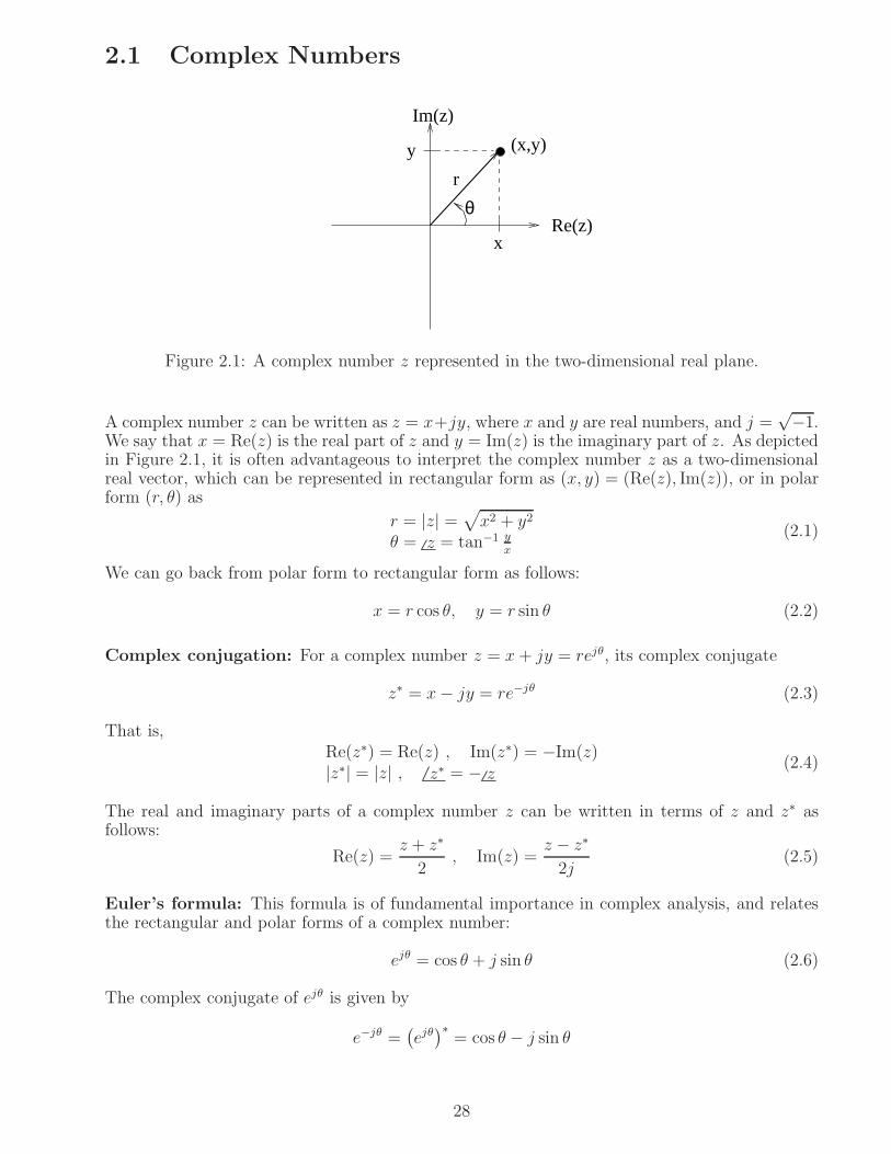
Figure 2.1: A complex number z represented in the two-dimensional real plane.

A complex number z can be written as z = x+jy, where x and y are real numbers, and j =√−1.

We say that x = Re(z) is the real part of z and y = Im(z) is the imaginary part of z. As depictedin Figure 2.1, it is often advantageous to interpret the complex number z as a two-dimensionalreal vector, which can be represented in rectangular form as (x, y) = (Re(z), Im(z)), or in polarform (r, θ) as

r = |z| =√

x2 + y2

θ = z = tan−1 yx

(2.1)

We can go back from polar form to rectangular form as follows:

x = r cos θ, y = r sin θ (2.2)

Complex conjugation: For a complex number z = x+ jy = rejθ, its complex conjugate

z∗ = x− jy = re−jθ (2.3)

That is,Re(z∗) = Re(z) , Im(z∗) = −Im(z)|z∗| = |z| , z∗ = − z

(2.4)

The real and imaginary parts of a complex number z can be written in terms of z and z∗ asfollows:

Re(z) =z + z∗

2, Im(z) =

z − z∗

2j(2.5)

Euler’s formula: This formula is of fundamental importance in complex analysis, and relatesthe rectangular and polar forms of a complex number:

ejθ = cos θ + j sin θ (2.6)

The complex conjugate of ejθ is given by

e−jθ =(

ejθ)∗

= cos θ − j sin θ

28

We can express cosines and sines in terms of ejθ and its complex conjugate as follows:

Re(

ejθ)

=ejθ + e−jθ

2= cos θ , Im

(

ejθ)

=ejθ − e−jθ

2j= sin θ (2.7)

Applying Euler’s formula to (2.1), we can write

z = x+ jy = r cos θ + jr sin θ = rejθ (2.8)

Being able to go back and forth between the rectangular and polar forms of a complex numberis useful. For example, it is easier to add in the rectangular form, but it is easier to multiply inthe polar form.

Complex Addition: For two complex numbers z1 = x1 + jy1 and z2 = x2 + jy2,

z1 + z2 = (x1 + x2) + j(y1 + y2) (2.9)

That is,Re(z1 + z2) = Re(z1) + Re(z2) , Im(z1 + z2) = Im(z1) + Im(z2) (2.10)

Complex Multiplication (rectangular form): For two complex numbers z1 = x1 + jy1 andz2 = x2 + jy2,

z1z2 = (x1x2 − y1y2) + j(y1x2 + x1y2) (2.11)

This follows simply by multiplying out, and setting j2 = −1. We have

Re(z1z2) = Re(z1)Re(z2)− Im(z1)Im(z2) , Im(z1z2) = Im(z1)Re(z2) + Re(z1)Im(z2) (2.12)

Note that, using the rectangular form, a single complex multiplication requires four real multi-plications.

Complex Multiplication (polar form): Complex multiplication is easier when the numbersare expressed in polar form. For z1 = r1e

jθ1, z2 = r2ejθ2 , we have

z1z2 = r1r2ej(θ1+θ2) (2.13)

That is,|z1z2| = |z1||z2| , z1z2 = z1 + z2 (2.14)

Division: For two complex numbers z1 = x1 + jy1 = r1ejθ1 and z2 = x2 + jy2 = r2e

jθ2 (withz2 6= 0, i.e., r2 > 0), it is easiest to express the result of division in polar form:

z1/z2 = (r1/r2)ej(θ1−θ2) (2.15)

That is,|z1/z2| = |z1|/|z2| , z1/z2 = z1 − z2 (2.16)

In order to divide using rectangular form, it is convenient to multiply numerator and denominatorby z∗2 , which gives

z1/z2 = z1z∗2/(z2z

∗2) = z1z

∗2/|z2|2 =

(x1 + jy1)(x2 − jy2)

x22 + y22

Multiplying out as usual, we get

z1/z2 =(x1x2 + y1y2) + j (−x1y2 + y1x2)

x22 + y22(2.17)

29

Example 2.1.1 (Computations with complex numbers) Consider the complex numbersz1 = 1 + j and z2 = 2e−jπ/6. Find z1 + z2, z1z2, and z1/z2. Also specify z∗1 , z

∗2 .

For complex addition, it is convenient to express both numbers in rectangular form. Thus,

z2 = 2 (cos(−π/6) + j sin(−π/6)) =√3− j

andz1 + z2 = (1 + j) + (

√3− j) =

√3 + 1

For complex multiplication and division, it is convenient to express both numbers in polar form.We obtain z1 =

√2ejπ/4 by applying (2.1). Now, from (2.11), we have

z1z2 =√2ejπ/42e−jπ/6 = 2

√2ej(π/4−π/6) = 2

√2ejπ/12

Similarly,

z1/z2 =

√2ejπ/4

2e−jπ/6=

1√2ej(π/4+π/6) =

1√2ej5π/12

Multiplication using the rectangular forms of the complex numbers yields the following:

z1z2 = (1 + j)(√3− j) =

√3− j +

√3j + 1 =

(√3 + 1

)

+ j(√

3− 1)

Note that z∗1 = 1 − j =√2e−jπ/4 and z∗2 = 2ejπ/6 =

√3 + j. Division using rectangular forms

gives

z1/z2 = z1z∗2/|z2|2 = (1 + j)(

√3 + j)/22 =

√3− 1

4+ j

√3 + 1

4

No need to memorize trigonometric identities any more: Once we can do computationsusing complex numbers, we can use Euler’s formula to quickly derive well-known trigonometricidentities involving sines and cosines. For example,

cos(θ1 + θ2) = Re(

ej(θ1+θ2))

Butej(θ1+θ2) = ejθ1ejθ2 = (cos θ1 + j sin θ1) (cos θ2 + j sin θ2)

= (cos θ1 cos θ2 − sin θ1 sin θ2) + j (cos θ1 sin θ2 + sin θ1 cos θ2)

Taking the real part, we can read off the identity

cos(θ1 + θ2) = cos θ1 cos θ2 − sin θ1 sin θ2 (2.18)

Moreover, taking the imaginary part, we can read off

sin(θ1 + θ2) = cos θ1 sin θ2 + sin θ1 cos θ2 (2.19)

2.2 Signals

Signal: A signal s(t) is a function of time (or some other independent variable, such as fre-quency, or spatial coordinates) which has an interesting physical interpretation. For example, itis generated by a transmitter, or processed by a receiver. While physically realizable signals suchas those sent over a wire or over the air must take real values, we shall see that it is extremely

30

useful (and physically meaningful) to consider a pair of real-valued signals, interpreted as thereal and imaginary parts of a complex-valued signal. Thus, in general, we allow signals to takecomplex values.

Discrete versus Continuous Time: We generically use the notation x(t) to denote continuoustime signals (t taking real values), and x[n] to denote discrete time signals (n taking integervalues). A continuous time signal x(t) sampled at rate Ts produces discrete time samples x(nTs+t0) (t0 an arbitrary offset), which we often denote as a discrete time signal x[n]. While signalssent over a physical communication channel are inherently continuous time, implementations atboth the transmitter and receiver make heavy use of discrete time implementations on digitizedsamples corresponding to the analog continuous time waveforms of interest.

We now introduce some signals that recur often in this text.

Sinusoid: This is a periodic function of time of the form

s(t) = A cos(2πf0t+ θ) (2.20)

where A > 0 is the amplitude, f0 is the frequency, and θ∈ [0, 2π] is the phase. By setting θ = 0,we obtain a pure cosine A cos 2πfct, and by setting θ = −π

2, we obtain a pure sine A sin 2πfct.

In general, using (2.18), we can rewrite (2.20) as

s(t) = Ac cos 2πf0t−As sin 2πf0t (2.21)

where Ac = A cos θ and As = A sin θ are real numbers. Using Euler’s formula, we can write

Aejθ = Ac + jAs (2.22)

Thus, the parameters of a sinusoid at frequency f0 can be represented by the complex number in(2.22), with (2.20) using the polar form, and (2.21) the rectangular form, of this number. Note

that A =√

A2c + A2

s and θ = tan−1 As

Ac.

Clearly, sinusoids with known amplitude, phase and frequency are perfectly predictable, andhence cannot carry any information. As we shall see, information can be transmitted by makingthe complex number Aejθ = Ac + jAs associated with the parameters of sinusoid vary in a waythat depends on the message to be conveyed. Of course, once this is done, the resulting signalwill no longer be a pure sinusoid, and part of the work of the communication system designer isto decide what shape such a signal should take in the frequency domain.

We now define complex exponentials, which play a key role in understanding signals and systemsin the frequency domain.

Complex exponential: A complex exponential at a frequency f0 is defined as

s(t) = Aej(2πf0t+θ) = αej2πf0t (2.23)

where A > 0 is the amplitude, f0 is the frequency, θ∈ [0, 2π] is the phase, and α = Aejθ is acomplex number that contains both the amplitude and phase information. Let us now makethree observations. First, note the ease with which we handle amplitude and phase for complexexponentials: they simply combine into a complex number that factors out of the complexexponential. Second, by Euler’s formula,

Re(

Aej(2πf0t+θ))

= A cos(2πf0t+ θ)

so that real-valued sinusoids are “contained in” complex exponentials. Third, as we shall soonsee, the set of complex exponentials ej2πft, where f takes values in (−∞,∞), form a “basis”for a large class of signals (basically, for all signals that are of interest to us), and the Fouriertransform of a signal is simply its expansion with respect to this basis. Such observations are

31

a/2

1/a

a

1/a

t t−a−a/2

Figure 2.2: The impulse function may be viewed as a limit of tall thin pulses (a → 0 in theexamples shown in the figure).

Unit area

0

t − a0 1 t + a0 2

s(t)

p(t)

tt

Figure 2.3: Multiplying a signal with a tall thin pulse to select its value at t0.

key to why complex exponentials play such an important role in signals and systems in general,and in communication systems in particular.

The Delta, or Impulse, Function: Another signal that plays a crucial role in signals and sys-tems is the delta function, or the unit impulse, which we denote by δ(t). Physically, we can thinkof it as a narrow, tall pulse with unit area: examples are shown in Figure 2.2. Mathematically,we can think of it as a limit of such pulses as the pulse width shrinks (and hence the pulse heightgoes to infinity). Such a limit is not physically realizable, but it serves a very useful purpose interms of understanding the structure of physically realizable signals. That is, consider a signals(t) that varies smoothly, and multiply it with a tall, thin pulse of unit area, centered at timet0, as shown in Figure 2.3. If we now integrate the product, we obtain

∫ ∞

−∞s(t)p(t)dt =

∫ t0+a2

t0−a1

s(t)p(t)dt ≈ s(t0)

∫ t0+a1

t0−a1

p(t)dt = s(t0)

That is, the preceding operation “selects” the value of the signal at time t0. Taking the limit ofthe tall thin pulse as its width a1 + a2 → 0, we get a translated version of the delta function,namely, δ(t − t0). Note that the exact shape of the pulse does not matter in the precedingargument. The delta function is therefore defined by means of the following sifting property: forany “smooth” function s(t), we have

∫ ∞

−∞s(t)δ(t− t0)dt = s(t0) Sifting property of the impulse (2.24)

Thus, the delta function is defined mathematically by the way it acts on other signals, ratherthan as a signal by itself. However, it is also important to keep in mind its intuitive interpretationas (the limit of) a tall, thin, pulse of unit area.

32

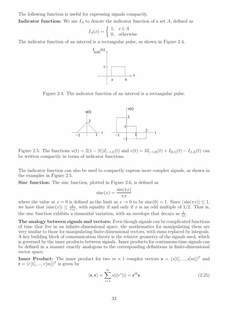
The following function is useful for expressing signals compactly.

Indicator function: We use IA to denote the indicator function of a set A, defined as

IA(x) =

1, x∈A0, otherwise

The indicator function of an interval is a rectangular pulse, as shown in Figure 2.4.

1

I (x)

a bx

[a,b]

Figure 2.4: The indicator function of an interval is a rectangular pulse.

t−1 1

21

3

−1

2

−1 1

u(t)v(t)

t

Figure 2.5: The functions u(t) = 2(1− |t|)I[−1,1](t) and v(t) = 3I[−1,0](t) + I[0,1](t)− I[1,2](t) canbe written compactly in terms of indicator functions.

The indicator function can also be used to compactly express more complex signals, as shown inthe examples in Figure 2.5.

Sinc function: The sinc function, plotted in Figure 2.6, is defined as

sinc(x) =sin(πx)

πx

where the value at x = 0 is defined as the limit as x→ 0 to be sinc(0) = 1. Since | sin(πx)| ≤ 1,we have that |sinc(x)| ≤ 1

π|x| , with equality if and only if x is an odd multiple of 1/2. That is,

the sinc function exhibits a sinusoidal variation, with an envelope that decays as 1|x| .

The analogy between signals and vectors: Even though signals can be complicated functionsof time that live in an infinite-dimensional space, the mathematics for manipulating them arevery similar to those for manipulating finite-dimensional vectors, with sums replaced by integrals.A key building block of communication theory is the relative geometry of the signals used, whichis governed by the inner products between signals. Inner products for continuous-time signals canbe defined in a manner exactly analogous to the corresponding definitions in finite-dimensionalvector space.

Inner Product: The inner product for two m × 1 complex vectors s = (s[1], ..., s[m])T andr = (r[1], ..., r[m])T is given by

〈s, r〉 =m∑

i=1

s[i]r∗[i] = rHs (2.25)

33

−5 −4 −3 −2 −1 0 1 2 3 4 5−0.4

−0.2

0

0.2

0.4

0.6

0.8

1

x

sinc

(x)

Figure 2.6: The sinc function.

Similarly, we define the inner product of two (possibly complex-valued) signals s(t) and r(t) asfollows:

〈s, r〉 =∫ ∞

−∞s(t)r∗(t) dt (2.26)

The inner product obeys the following linearity properties:

〈a1s1 + a2s2, r〉 = a1〈s1, r〉+ a2〈s2, r〉〈s, a1r1 + a2r2〉 = a∗1〈s, r1〉+ a∗2〈s, r2〉

where a1, a2 are complex-valued constants, and s, s1, s2, r, r1, r2 are signals (or vectors). Thecomplex conjugation when we pull out constants from the second argument of the inner productis something that we need to maintain awareness of when computing inner products for complex-valued signals.

Energy and Norm: The energy Es of a signal s is defined as its inner product with itself:

Es = ||s||2 = 〈s, s〉 =∫ ∞

−∞|s(t)|2dt (2.27)

where ||s|| denotes the norm of s. If the energy of s is zero, then s must be zero “almosteverywhere” (e.g., s(t) cannot be nonzero over any interval, no matter how small its length).For continuous-time signals, we take this to be equivalent to being zero everywhere. With thisunderstanding, ||s|| = 0 implies that s is zero, which is a property that is true for norms infinite-dimensional vector spaces.

Example 2.2.1 (Energy computations) Consider s(t) = 2I[0,T ] + jI[T/2,2T ]. Writing it out inmore detail, we have

s(t) =

2, 0 ≤ t < T/22 + j, T/2 ≤ t < Tj, T ≤ t < 2T

so that its energy is given by

||s||2 =∫ T/2

0

22dt+

∫ T

T/2

|2 + j|2dt+∫ 2T

T

|j|2dt = 4(T/2) + 5(T/2) + T = 11T/2

34

As another example, consider s(t) = e−3|t|+j2πt, for which the energy is given by

||s||2 =∫ ∞

−∞|e−3|t|+j2πt|2dt =

∫ ∞

−∞e−6|t|dt = 2

∫ ∞

0

e−6tdt = 1/3

Note that the complex phase term j2πt does not affect the energy, since it goes away when wetake the magnitude.

Power: The power of a signal s(t) is defined as the time average of its energy computed over alarge time interval:

Ps = limTo→∞

1

To

∫ To2

−To2

|s(t)|2dt (2.28)

Finite energy signals, of course, have zero power.

We see from (2.28) that power is defined as a time average. It is useful to introduce a compactnotation for time averages.

Time average: For a function g(t), define the time average as

g = limTo→∞

1

To

∫ To2

−To2

g(t)dt (2.29)

That is, we compute the time average over an observation interval of length To, and then letthe observation interval get large. We can now rewrite the power computation in (2.28) in thisnotation as follows.

Power: The power of a signal s(t) is defined as

Ps = |s(t)|2 (2.30)

Another time average of interest is the DC value of a signal.

DC value: The DC value of s(t) is defined as s(t).

Let us compute these quantities for the simple example of a complex exponential, s(t) =Aej(2πf0t+θ), where A > 0 is the amplitude, θ∈ [0, 2π] is the phase, and f0 is a real-valuedfrequency. Since |s(t)|2 ≡ A2 for all t, we get the same value when we average it. Thus, the

power is given by Ps = s2(t) = A2. For nonzero frequency f0, it is intuitively clear that all thepower in s is concentrated away from DC, since s(t) = Aej(2πf0t+θ) ↔ S(f) = Aejθδ(f − f0).We therefore see that the DC value is zero. While this is a convincing intuitive argument, it isinstructive to prove this starting from the definition (2.29).

Proving that a complex exponential has zero DC value: For s(t) = Aej(2πf0t+θ), theintegral over its period (of length 1/f0) is zero. As shown in Figure 2.7, the length L of anyinterval I can be written as L = K/f0 + ℓ where K is a nonnegative integer and 0 ≤ ℓ < 1

f0is

the length of the remaining interval Ir. Since the integral over an integer number of periods iszero, we have

∫

I

s(t)dt =

∫

Ir

s(t)dt

Thus,

|∫

I

s(t)dt| = |∫

Ir

s(t)dt| ≤ ℓ maxt|s(t)| = Aℓ <A

f0

35

]

I

1/f 0

0K/f

IrInterval (length )l

[

Interval

Figure 2.7: The interval I for computing the time average of a periodic function with period1/f0 can be decomposed into an integer number K of periods, with the remaining interval Ir oflength ℓ < 1

f0.

since |s(t)| = A. We therefore obtain

|∫ To

2

−To2

s(t)dt| ≤ (A/f0)

which yields that the DC value s = 0, since

|s| = | limTo→∞

1

To

∫ To2

−To2

s(t)dt| ≤ limTo→∞

A

f0To= 0

Essentially the same argument implies that, in general, the time average of a periodic signalequals the average over a single period. We use this fact without further comment henceforth.

Power and DC value of a sinusoid: For a real-valued sinusoid s(t) = A cos(2πf0t + θ), wecan use the results derived for complex exponentials above. Using Euler’s identity, a real-valuedsinusoid at f0 is a sum of complex exponentials at ±f0:

s(t) =A

2ej(2πf0t+θ) +

A

2e−j(2πf0t+θ)

Since each complex exponential has zero DC value, we obtain

s = 0

That is, the DC value of any real-valued sinusoid is zero.

Ps = s2(t) = A2 cos2(2πf0t + θ) =A2

2+A2

2cos(4πf0t+ 2θ) =

A2

2

since the DC value of the sinusoid at 2f0 is zero.

2.3 Linear Time Invariant Systems

System: A system takes as input one or more signals, and produces as output one or moresignals. A system is specified once we characterize its input-output relationship; that is, if wecan determine the output, or response, y(t), corresponding to any possible input x(t) in a givenclass of signals of interest.

36

Our primary focus here is on linear time invariant (LTI) systems, which provide good modelsfor filters at the transmitter and receiver, as well as for the distortion induced by a variety ofchannels. We shall see that the input-output relationship is particularly easy to characterize forsuch systems.

Linear system: Let x1(t) and x2(t) denote arbitrary input signals, and let y1(t) and y2(t)denote the corresponding system outputs, respectively. Then, for arbitrary scalars a1 and a2, theresponse of the system to input a1x1(t) + a2x2(t) is a1y1(t) + a2y2(t).

Time invariant system: Let y(t) denote the system response to an input x(t). Then thesystem response to a time-shifted version of the input, x1(t) = x(t− t0) is y1(t) = y(t− t0). Thatis, a time shift in the input causes an identical time shift in the output.

Example 2.3.1 Examples of linear systems It can (and should) be checked that the followingsystems are linear. These examples show that linear systems may or may not be time invariant.

y(t) = 2x(t− 1)− jx(t− 2) time invariant

y(t) = (3− 2j)x(1− t) time varying

y(t) = x(t) cos(100πt)− x(t− 1) sin(100πt) time varying

y(t) =

∫ t+1

t−1

x(τ)dτ time invariant

Example 2.3.2 Examples of time invariant systems It can (and should) be checked thatthe following systems are time invariant. These examples show that time invariant systems mayor may not be linear.

y(t) = e2x(t−1) nonlinear

y(t) =

∫ t

−∞x(τ)e−(t−τ)dτ linear

y(t) =

∫ t+1

t−1

x2(τ)dτ nonlinear

Linear time invariant system: A linear time invariant (LTI) system is (unsurprisingly) definedto be a system which is both linear and time invariant. What is surprising, however, is howpowerful the LTI property is in terms of dictating what the input-output relationship must looklike. Specifically, if we know the impulse response of an LTI system (i.e., the output signalwhen the input signal is the delta function), then we can compute the system response for anyinput signal. Before deriving and stating this result, we illustrate the LTI property using anexample; see Figure 2.8. Suppose that the response of an LTI system to the rectangular pulsep1(t) = I[− 1

2, 12](t) is given by the trapezoidal waveform h1(t). We can now compute the system

response to any linear combination of time shifts of the pulse p(t), as illustrated by the examplein the figure. More generally, using the LTI property, we infer that the response to an inputsignal of the form x(t) =

∑

i aip1(t− ti) is y(t) =∑

i aih1(t− ti).

Can we extend the preceding idea to compute the system response to arbitrary input signals?The answer is yes: if we know the system response to thinner and thinner pulses, then wecan approximate arbitrary signals better and better using linear combinations of shifts of thesepulses. Consider p∆(t) =

1∆I[−∆

2,∆2](t), where ∆ > 0 is getting smaller and smaller. Note that we

have normalized the area of the pulse to unity, so that the limit of p∆(t) as ∆ → 0 is the delta

37

1

1

−1

1 4

2h (t)1

2

30

y(t)

t1 2

3 4

−1

2

0

S

S

h (t)1

t1 2 30

11

p (t)

+=

1

t−0.5 0.5

2

t−0.5

1.5

−1

x(t) = 2 p (t) − p (t−1)1

−h (t−1)

Figure 2.8: Given that the response of an LTI system S to the pulse p1(t) is h1(t), we can use theLTI property to infer that the response to x(t) = 2p1(t)− p1(t− 1) is y(t) = 2h1(t)− h1(t− 1).

t

... ...

∆

x(t)

Figure 2.9: A smooth signal can be approximated as a linear combination of shifts of tall thinpulses.

38

function. Figure 2.9 shows how to approximate a smooth input signal as a linear combination ofshifts of p∆(t). That is, for ∆ small, we have

x(t) ≈ x∆(t) =∞∑

k=−∞x(k∆)∆p∆(t− k∆) (2.31)

If the system response to p∆(t) is h∆(t), then we can use the LTI property to compute theresponse y∆(t) to x∆(t), and use this to approximate the response y(t) to the input x(t), asfollows:

y(t) ≈ y∆(t) =

∞∑

k=−∞x(k∆)∆h∆(t− k∆) (2.32)

As ∆ → 0, the sums above tend to integrals, and the pulse p∆(t) tends to the delta function δ(t).The approximation to the input signal in equation (2.31) becomes exact, with the sum tendingto an integral:

lim∆→0

x∆(t) = x(t) =

∫ ∞

−∞x(τ)δ(t− τ)dτ

replacing the discrete time shifts k∆ by the continuous variable τ , the discrete increment ∆ bythe infinitesimal dτ , and the sum by an integral. This is just a restatement of the sifting propertyof the impulse. That is, an arbitrary input signal can be expressed as a linear combination oftime-shifted versions of the delta function, where we now consider a continuum of time shifts.

In similar fashion, the approximation to the output signal in (2.32) becomes exact, with the sumreducing to the following convolution integral:

lim∆→0

y∆(t) = y(t) =

∫ ∞

−∞x(τ)h(t− τ)dτ (2.33)

where h(t) denotes the impulse response of the LTI system.

Convolution and its computation: The convolution v(t) of two signals u1(t) and u2(t) isgiven by

v(t) = (u1 ∗ u2)(t) =∫ ∞

−∞u1(τ)u2(t− τ) dτ =

∫ ∞

−∞u1(t− τ)u2(τ) dτ (2.34)

Note that τ is a dummy variable that is integrated out in order to determine the value of thesignal v(t) at each possible time t. The role of u1 and u2 in the integral can be exchanged. Thiscan be proved using a change of variables, replacing t− τ by τ . We often drop the time variable,and write v = u1 ∗ u2 = u2 ∗ u1.An LTI system is completely characterized by its impulse response: As derived in(2.33), the output y of an LTI system is the convolution of the input signal u and the systemimpulse response h. That is, y = u∗h. From (2.34), we realize that the role of the signal and thesystem can be exchanged: that is, we would get the same output y if a signal h is sent througha system with impulse response u.

Flip and slide: Consider the expression for the convolution in (2.34):

v(t) =

∫ ∞

−∞u1(τ)u2(t− τ) dτ

Fix a value of time t at which we wish to evaluate v. In order to compute v(t), we must multiplytwo functions of a “dummy variable” τ and then integrate over τ . In particular, s2(τ) = u2(−τ)is the signal u2(τ) flipped around the origin, so that u2(t − τ) = u2(−(τ − t)) = s2(τ − t) iss2(τ) translated to the right by t (if t < 0, translation to the right by t actually corresponds to

39

translation is to the left by |t|). In short, the mechanics of computing the convolution involvesflipping and sliding one of the signals, multiplying with the other signal, and integrating. Picturesare extremely helpful when doing such computations by hand, as illustrated by the followingexample.

depicted in (a)−(e)

1 τ

u (t− )τ2

u (t− )τ2

u (t− )τ2

u (t− )τ2

u (t− )τ2

u (− )τ2

−3 −1τ

τ2u ( )

τ

τ

τ

τ

τ

τ5 11

t−3 t−1

t−3 t−1

t−3

t−3

t−3

t−1

t−1

t−1

(a) t−1 < 5

(b) t−3 < 5, t−1 > 5

(c) t−3 > 5, t−1 < 11

(d) t−3 < 11, t−1 > 11

(e) t−3 > 11

τ31

Flip

Different ranges of t

Slide by t

u ( )

Figure 2.10: Illustrating the flip and slide operation for the convolution of two rectangular pulses.

t

v(t)

2

6 8 12 14

Figure 2.11: The convolution of the two rectangular pulses in Example 2.3.3 results in a trape-zoidal pulse.

Example 2.3.3 Convolving rectangular pulses: Consider the rectangular pulses u1(t) =I[5,11](t) and u2(t) = I[1,3](t). We wish to compute the convolution

v(t) = (u1 ∗ u2)(t) =∫ ∞

−∞u1(τ)u2(t− τ)dτ

We now draw pictures of the signals involved in these “flip and slide” computations in order tofigure out the limits of integration for different ranges of t. Figure 2.10 shows that there are fivedifferent ranges of interest, and yields the following result:(a) For t < 6, u1(τ)u2(t− τ) ≡ 0, so that v(t) = 0.(b) For 6 < t < 8, u1(τ)u2(t− τ) = 1 for 5 < τ < t− 1, so that

v(t) =

∫ t−1

5

dτ = t− 6

40

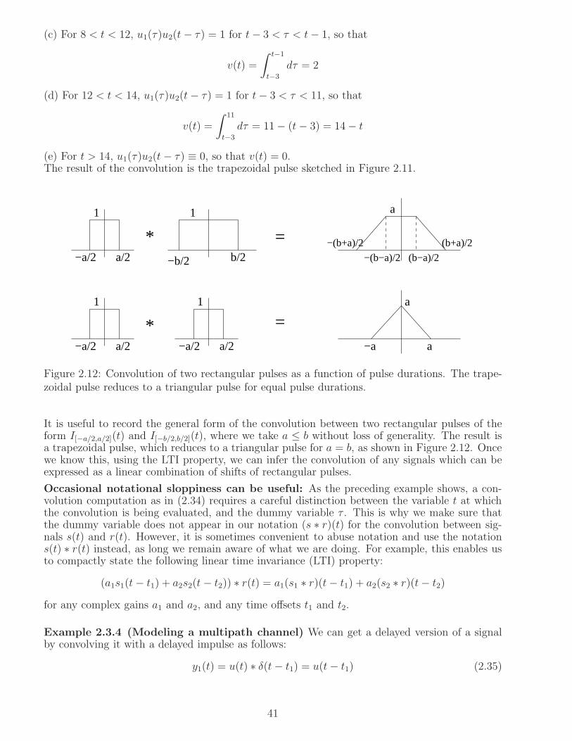
(c) For 8 < t < 12, u1(τ)u2(t− τ) = 1 for t− 3 < τ < t− 1, so that

v(t) =

∫ t−1

t−3

dτ = 2

(d) For 12 < t < 14, u1(τ)u2(t− τ) = 1 for t− 3 < τ < 11, so that

v(t) =

∫ 11

t−3

dτ = 11− (t− 3) = 14− t

(e) For t > 14, u1(τ)u2(t− τ) ≡ 0, so that v(t) = 0.The result of the convolution is the trapezoidal pulse sketched in Figure 2.11.

−(b+a)/2

−a/2 a/2

1

−a/2 a/2

1

−a/2 a/2

1

b/2−b/2

* =

1 a

* =−a a

a

(b−a)/2−(b−a)/2

(b+a)/2

Figure 2.12: Convolution of two rectangular pulses as a function of pulse durations. The trape-zoidal pulse reduces to a triangular pulse for equal pulse durations.

It is useful to record the general form of the convolution between two rectangular pulses of theform I[−a/2,a/2](t) and I[−b/2,b/2](t), where we take a ≤ b without loss of generality. The result isa trapezoidal pulse, which reduces to a triangular pulse for a = b, as shown in Figure 2.12. Oncewe know this, using the LTI property, we can infer the convolution of any signals which can beexpressed as a linear combination of shifts of rectangular pulses.

Occasional notational sloppiness can be useful: As the preceding example shows, a con-volution computation as in (2.34) requires a careful distinction between the variable t at whichthe convolution is being evaluated, and the dummy variable τ . This is why we make sure thatthe dummy variable does not appear in our notation (s ∗ r)(t) for the convolution between sig-nals s(t) and r(t). However, it is sometimes convenient to abuse notation and use the notations(t) ∗ r(t) instead, as long we remain aware of what we are doing. For example, this enables usto compactly state the following linear time invariance (LTI) property:

(a1s1(t− t1) + a2s2(t− t2)) ∗ r(t) = a1(s1 ∗ r)(t− t1) + a2(s2 ∗ r)(t− t2)

for any complex gains a1 and a2, and any time offsets t1 and t2.

Example 2.3.4 (Modeling a multipath channel) We can get a delayed version of a signalby convolving it with a delayed impulse as follows:

y1(t) = u(t) ∗ δ(t− t1) = u(t− t1) (2.35)

41

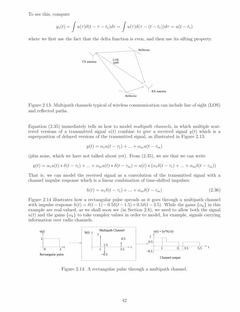
To see this, compute

y1(t) =

∫

u(τ)δ(t− τ − t1)dτ =

∫

u(τ)δ(τ − (t− t1))dτ = u(t− t1)

where we first use the fact that the delta function is even, and then use its sifting property.

Reflector

TX antenna

RX antenna

pathLOS

Reflector

Figure 2.13: Multipath channels typical of wireless communication can include line of sight (LOS)and reflected paths.

Equation (2.35) immediately tells us how to model multipath channels, in which multiple scat-tered versions of a transmitted signal u(t) combine to give a received signal y(t) which is asuperposition of delayed versions of the transmitted signal, as illustrated in Figure 2.13:

y(t) = α1u(t− τ1) + ...+ αmu(t− τm)

(plus noise, which we have not talked about yet). From (2.35), we see that we can write

y(t) = α1u(t) ∗ δ(t− τ1) + ...+ αmu(t) ∗ δ(t− τm) = u(t) ∗ (α1δ(t− τ1) + ...+ αmδ(t− τm))

That is, we can model the received signal as a convolution of the transmitted signal with achannel impulse response which is a linear combination of time-shifted impulses:

h(t) = α1δ(t− τ1) + ... + αmδ(t− τm) (2.36)

Figure 2.14 illustrates how a rectangular pulse spreads as it goes through a multipath channelwith impulse response h(t) = δ(t−1)−0.5δ(t−1.5)+0.5δ(t−3.5). While the gains αk in thisexample are real-valued, as we shall soon see (in Section 2.8), we need to allow both the signalu(t) and the gains αk to take complex values in order to model, for example, signals carryinginformation over radio channels.

y(t) = (u*h) (t)1

−0.5

0.5

11.5

3.5t

h(t)

Rectangular pulse

t0 2

1

Channel output

Multipath Channelu(t)

t1 3 5.53.5

1

0.5

−0.5

Figure 2.14: A rectangular pulse through a multipath channel.

42

H(f ) π 0ej2 f tπ 0e LTI System0

j2 f t

Figure 2.15: Complex exponentials are eigenfunctions of LTI systems.

Complex exponential through an LTI system: In order to understand LTI systems in thefrequency domain, let us consider what happens to a complex exponential u(t) = ej2πf0t when itgoes through an LTI system with impulse response h(t). The output is given by

y(t) = (u ∗ h)(t) =∫∞−∞ h(τ)ej2πf0(t−τ)dτ

= ej2πf0t∫∞−∞ h(τ)e−j2πf0τdτ = H(f0)e

j2πf0t

(2.37)

where

H(f0) =

∫ ∞

−∞h(τ)e−j2πf0τdτ

is the Fourier transform of h evaluated at the frequency f0. We discuss the Fourier transformand its properties in more detail shortly.

Complex exponentials are eigenfunctions of LTI systems: Recall that an eigenvector ofa matrix H is any vector x that satisfies Hx = λx. That is, the matrix leaves its eigenvectorsunchanged except for a scale factor λ, which is the eigenvalue associated with that eigenvector.In an entirely analogous fashion, we see that the complex exponential signal ej2πf0t is an eigen-function of the LTI system with impulse response h, with eigenvalue H(f0). Since we have notconstrained h, we conclude that complex exponentials are eigenfunctions of any LTI system. Weshall soon see, when we discuss Fourier transforms, that this eigenfunction property allows usto characterize LTI systems in the frequency domain, which in turn enables powerful frequencydomain design and analysis tools.

2.3.1 Discrete time convolution

DSP-based implementations of convolutions are inherent discrete time. For two discrete timesequences u1[n] and u2[n], their convolution y = u1 ∗ u2 is defined analogous to continuoustime convolution, replacing integration by summation:

y[n] =∑

k

u1[k]u2[n− k] (2.38)

Matlab implements this using the “conv” function. This can be interpreted as u1 being the inputto a system with impulse response u2, where a discrete time impulse is simply a one, followed byall zeros.

Continuous time convolution between u1(t) and u2(t) can be approximated using discrete timeconvolutions between the corresponding sampled signals. For example, for samples at rate 1/Ts,the infinitesimal dt is replaced by the sampling interval Ts as follows:

y(t) = (u1 ∗ u2)(t) =∫

u1(τ)u2(t− τ)dτ ≈∑

k

u1(kTs)u2(t− kTs)Ts

Evaluating at a sampling time t = nTs, we have

y(nTs) = Ts∑

k

u1(kTs)u2(nTs − kTs)

43

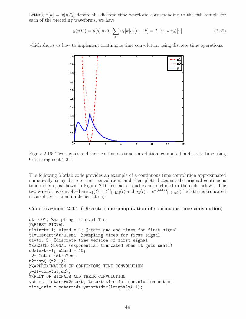
Letting x[n] = x(nTs) denote the discrete time waveform corresponding to the nth sample foreach of the preceding waveforms, we have

y(nTs) = y[n] ≈ Ts∑

k

u1[k]u2[n− k] = Ts(u1 ∗ u2)[n] (2.39)

which shows us how to implement continuous time convolution using discrete time operations.

−2 0 2 4 6 8 10 120

0.1

0.2

0.3

0.4

0.5

0.6

0.7

0.8

0.9

1

u1u2y

Figure 2.16: Two signals and their continuous time convolution, computed in discrete time usingCode Fragment 2.3.1.

The following Matlab code provides an example of a continuous time convolution approximatednumerically using discrete time convolution, and then plotted against the original continuoustime index t, as shown in Figure 2.16 (cosmetic touches not included in the code below). Thetwo waveforms convolved are u1(t) = t2I[−1,1](t) and u2(t) = e−(t+1)I[−1,∞) (the latter is truncatedin our discrete time implementation).

Code Fragment 2.3.1 (Discrete time computation of continuous time convolution)

dt=0.01; %sampling interval T_s%%FIRST SIGNALu1start=-1; u1end = 1; %start and end times for first signalt1=u1start:dt:u1end; %sampling times for first signalu1=t1.^2; %discrete time version of first signal%%SECOND SIGNAL (exponential truncated when it gets small)u2start=-1; u2end = 10;t2=u2start:dt:u2end;u2=exp(-(t2+1));%%APPROXIMATION OF CONTINUOUS TIME CONVOLUTIONy=dt*conv(u1,u2);%%PLOT OF SIGNALS AND THEIR CONVOLUTIONystart=u1start+u2start; %start time for convolution outputtime_axis = ystart:dt:ystart+dt*(length(y)-1);

44

%%PLOT u1, u2 and yplot(t1,u1,’r-.’);hold on;plot(t2,u2,’r:’);plot(time_axis,y);legend(’u1’,’u2’,’y’,’Location’,’NorthEast’);hold off;

2.3.2 Multi-rate systems

While continuous time signals can be converted to discrete time by sampling “fast enough,” it isoften required that we operate at multiple sampling rates. For example, in digital communication,we may send a string of symbols b[n] (think of these as taking values +1 or -1 for now) bymodulating them onto shifted versions of a pulse p(t) as follows:

u(t) =∑

n

b[n]p(t− nT ) (2.40)

where 1/T is the rate at which symbols are generated (termed the symbol rate). In order torepresent the analog pulse p(t) as discrete time samples, we may sample it at rate 1/Ts, typicallychosen to be an integer multiple of the symbol rate, so that T = mTs, where m is a positiveinteger. Typical values employed in transmitter DSP modules might be m = 4 or m = 8. Thus,the system we are interested is multi-rate: waveforms are sampled at rate 1/Ts = m/T , butthe input is at rate 1/T . Set u[k] = u(kTs) and p[k] = p(kTs) as the discrete time signalscorresponding to samples of the transmitted waveform u(t) and the pulse p(t), respectively. Wecan write the sampled version of (2.40) as

u[k] =∑

n

b[n]p(kTs − nT ) =∑

n

b[n]p[k − nm] (2.41)

The preceding almost has the form of a discrete time convolution, but the key difference isthat the successive symbols b[n] are spaced by time T , which corresponds to m > 1 samplesat the sampling rate 1/Ts. Thus, in order to implement this system using convolution at rate1/Ts, we must space out the input symbols by inserting m− 1 zeros between successive symbolsb[n], thus converting a rate 1/T signal to a rate 1/Ts = m/T signal. This process is termedupsampling. While the upsampling function is available in certain Matlab toolboxes, we providea self-contained code fragment below that illustrates its use for digital modulation, and plotsthe waveform obtained for symbol sequence −1,+1,+1,−1. The modulating pulse is a sinepulse: p(t) = sin(πt/T )I[0,T ], and our convention is to set T = 1 without loss of generality(or, equivalently, to replace t by t/T ). We set the oversampling factor M = 16 in order toobtain smooth plots, even though typical implementations in communication transmitters mayuse smaller values.

Code Fragment 2.3.2 (Upsampling for digital modulation)

m=16; %sampling rate as multiple of symbol rate%discrete time representation of sine pulsetime_p = 0:1/m:1; %sampling times over duration of pulsep = sin(pi*time_p); %samples of the pulse%symbols to be modulatedsymbols = [-1;1;1;-1];

45

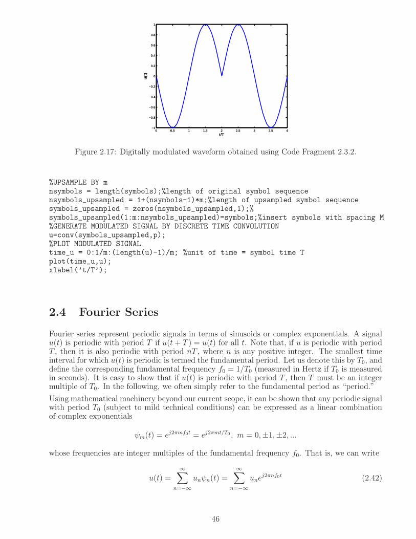
0 0.5 1 1.5 2 2.5 3 3.5 4−1

−0.8

−0.6

−0.4

−0.2

0

0.2

0.4

0.6

0.8

1

t/T

u(t)

Figure 2.17: Digitally modulated waveform obtained using Code Fragment 2.3.2.

%UPSAMPLE BY mnsymbols = length(symbols);%length of original symbol sequencensymbols_upsampled = 1+(nsymbols-1)*m;%length of upsampled symbol sequencesymbols_upsampled = zeros(nsymbols_upsampled,1);%symbols_upsampled(1:m:nsymbols_upsampled)=symbols;%insert symbols with spacing M%GENERATE MODULATED SIGNAL BY DISCRETE TIME CONVOLUTIONu=conv(symbols_upsampled,p);%PLOT MODULATED SIGNALtime_u = 0:1/m:(length(u)-1)/m; %unit of time = symbol time Tplot(time_u,u);xlabel(’t/T’);

2.4 Fourier Series

Fourier series represent periodic signals in terms of sinusoids or complex exponentials. A signalu(t) is periodic with period T if u(t+ T ) = u(t) for all t. Note that, if u is periodic with periodT , then it is also periodic with period nT , where n is any positive integer. The smallest timeinterval for which u(t) is periodic is termed the fundamental period. Let us denote this by T0, anddefine the corresponding fundamental frequency f0 = 1/T0 (measured in Hertz if T0 is measuredin seconds). It is easy to show that if u(t) is periodic with period T , then T must be an integermultiple of T0. In the following, we often simply refer to the fundamental period as “period.”

Using mathematical machinery beyond our current scope, it can be shown that any periodic signalwith period T0 (subject to mild technical conditions) can be expressed as a linear combinationof complex exponentials

ψm(t) = ej2πmf0t = ej2πmt/T0 , m = 0,±1,±2, ...

whose frequencies are integer multiples of the fundamental frequency f0. That is, we can write

u(t) =

∞∑

n=−∞unψn(t) =

∞∑

n=−∞une

j2πnf0t (2.42)

46

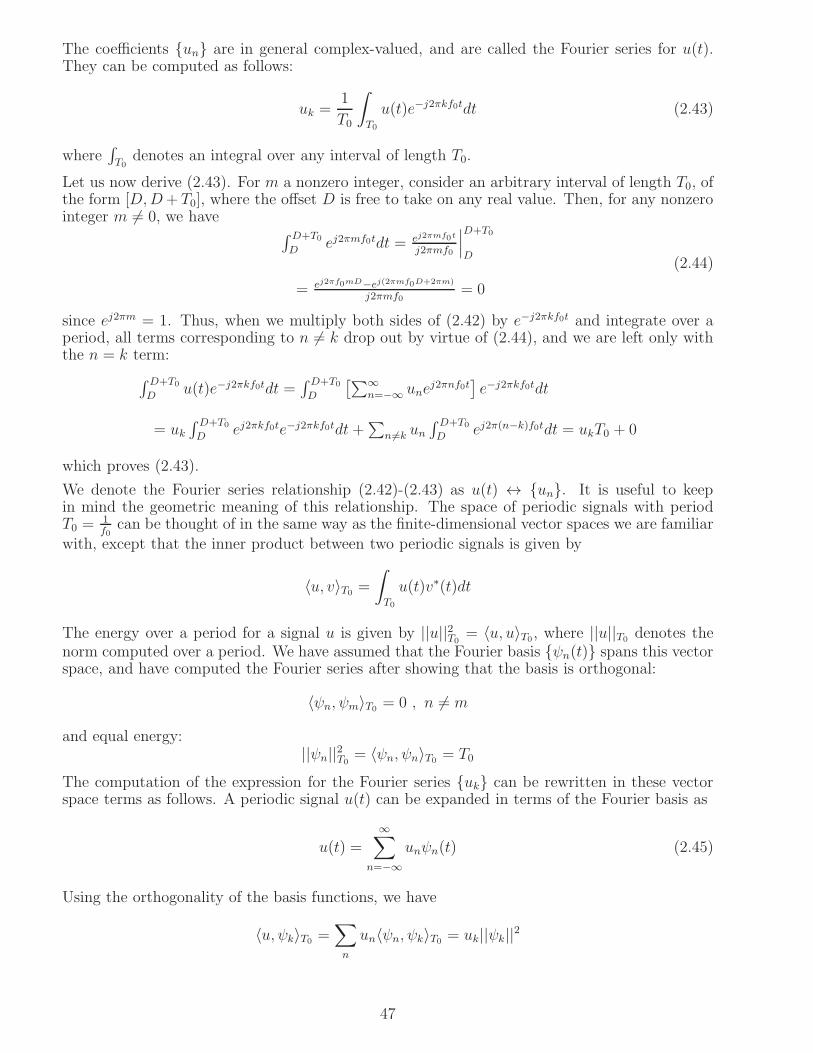
The coefficients un are in general complex-valued, and are called the Fourier series for u(t).They can be computed as follows:

uk =1

T0

∫

T0

u(t)e−j2πkf0tdt (2.43)

where∫

T0denotes an integral over any interval of length T0.

Let us now derive (2.43). For m a nonzero integer, consider an arbitrary interval of length T0, ofthe form [D,D+ T0], where the offset D is free to take on any real value. Then, for any nonzerointeger m 6= 0, we have

∫ D+T0

Dej2πmf0tdt = ej2πmf0t

j2πmf0

∣

∣

∣

D+T0

D

= ej2πf0mD−ej(2πmf0D+2πm)

j2πmf0= 0

(2.44)

since ej2πm = 1. Thus, when we multiply both sides of (2.42) by e−j2πkf0t and integrate over aperiod, all terms corresponding to n 6= k drop out by virtue of (2.44), and we are left only withthe n = k term:

∫ D+T0

Du(t)e−j2πkf0tdt =

∫ D+T0

D

[∑∞

n=−∞ unej2πnf0t

]

e−j2πkf0tdt

= uk∫ D+T0

Dej2πkf0te−j2πkf0tdt+

∑

n 6=k un∫ D+T0

Dej2π(n−k)f0tdt = ukT0 + 0

which proves (2.43).

We denote the Fourier series relationship (2.42)-(2.43) as u(t) ↔ un. It is useful to keepin mind the geometric meaning of this relationship. The space of periodic signals with periodT0 =

1f0

can be thought of in the same way as the finite-dimensional vector spaces we are familiar

with, except that the inner product between two periodic signals is given by

〈u, v〉T0 =

∫

T0

u(t)v∗(t)dt

The energy over a period for a signal u is given by ||u||2T0= 〈u, u〉T0, where ||u||T0 denotes the

norm computed over a period. We have assumed that the Fourier basis ψn(t) spans this vectorspace, and have computed the Fourier series after showing that the basis is orthogonal:

〈ψn, ψm〉T0 = 0 , n 6= m

and equal energy:||ψn||2T0

= 〈ψn, ψn〉T0 = T0

The computation of the expression for the Fourier series uk can be rewritten in these vectorspace terms as follows. A periodic signal u(t) can be expanded in terms of the Fourier basis as

u(t) =∞∑

n=−∞unψn(t) (2.45)

Using the orthogonality of the basis functions, we have

〈u, ψk〉T0 =∑

n

un〈ψn, ψk〉T0 = uk||ψk||2

47

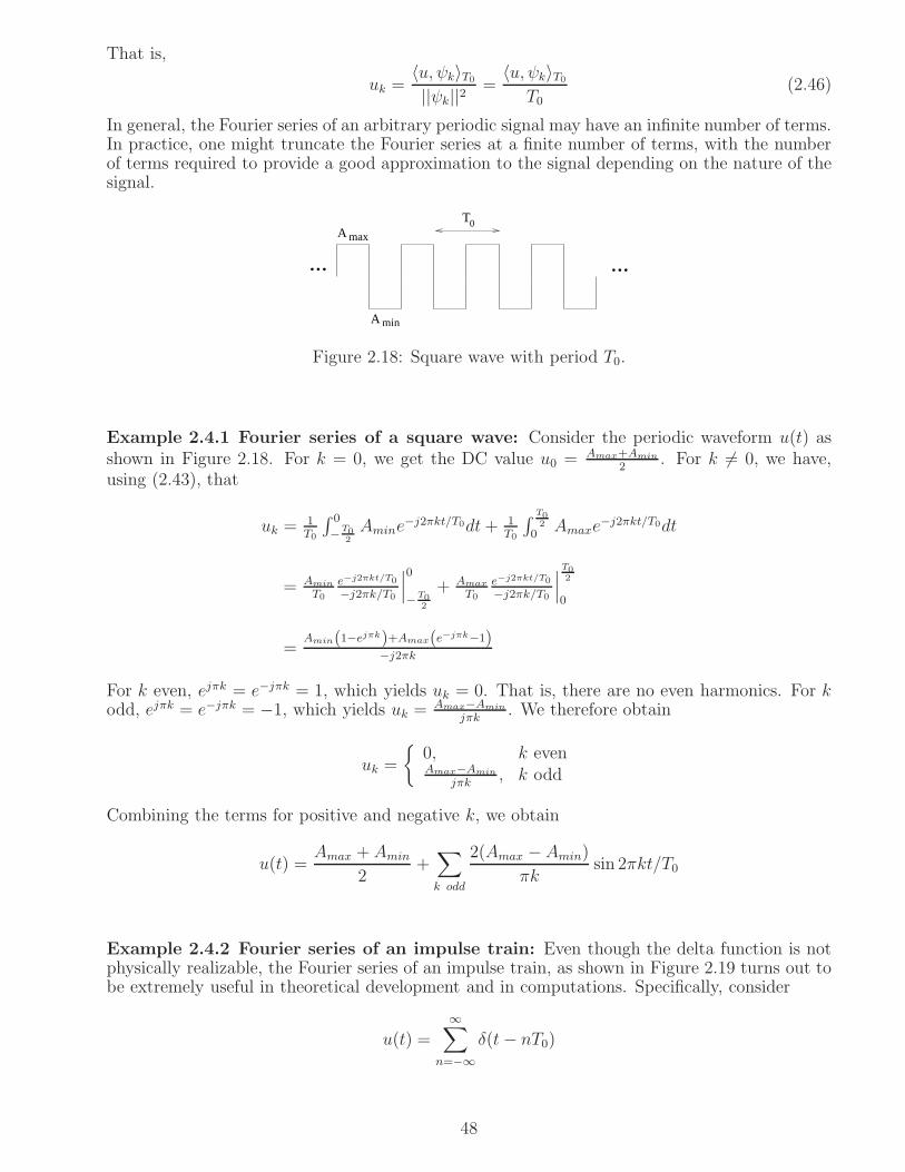
That is,

uk =〈u, ψk〉T0

||ψk||2=

〈u, ψk〉T0

T0(2.46)

In general, the Fourier series of an arbitrary periodic signal may have an infinite number of terms.In practice, one might truncate the Fourier series at a finite number of terms, with the numberof terms required to provide a good approximation to the signal depending on the nature of thesignal.

...max

A min

T0

...A

Figure 2.18: Square wave with period T0.

Example 2.4.1 Fourier series of a square wave: Consider the periodic waveform u(t) asshown in Figure 2.18. For k = 0, we get the DC value u0 = Amax+Amin

2. For k 6= 0, we have,

using (2.43), that

uk =1T0

∫ 0

−T02Amine

−j2πkt/T0dt+ 1T0

∫T02

0Amaxe

−j2πkt/T0dt

= Amin

T0

e−j2πkt/T0

−j2πk/T0

∣

∣

∣

0

−T02

+ Amax

T0

e−j2πkt/T0

−j2πk/T0

∣

∣

∣

T02

0

=Amin(1−ejπk)+Amax(e−jπk−1)

−j2πk

For k even, ejπk = e−jπk = 1, which yields uk = 0. That is, there are no even harmonics. For kodd, ejπk = e−jπk = −1, which yields uk =

Amax−Amin

jπk. We therefore obtain

uk =

0, k evenAmax−Amin

jπk, k odd

Combining the terms for positive and negative k, we obtain

u(t) =Amax + Amin

2+∑

k odd

2(Amax − Amin)

πksin 2πkt/T0

Example 2.4.2 Fourier series of an impulse train: Even though the delta function is notphysically realizable, the Fourier series of an impulse train, as shown in Figure 2.19 turns out tobe extremely useful in theoretical development and in computations. Specifically, consider

u(t) =

∞∑

n=−∞δ(t− nT0)

48

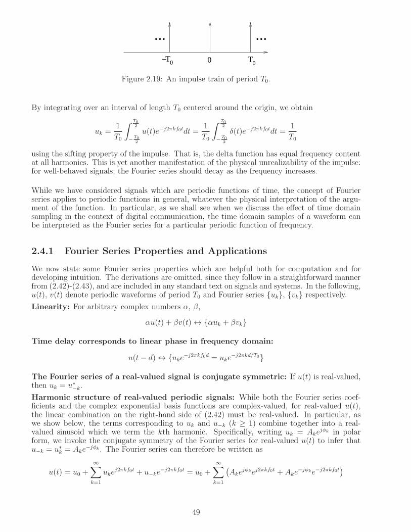
− 0T0

......

0 T

Figure 2.19: An impulse train of period T0.

By integrating over an interval of length T0 centered around the origin, we obtain

uk =1

T0

∫T02

−T02

u(t)e−j2πkf0tdt =1

T0

∫T02

−T02

δ(t)e−j2πkf0tdt =1

T0

using the sifting property of the impulse. That is, the delta function has equal frequency contentat all harmonics. This is yet another manifestation of the physical unrealizability of the impulse:for well-behaved signals, the Fourier series should decay as the frequency increases.

While we have considered signals which are periodic functions of time, the concept of Fourierseries applies to periodic functions in general, whatever the physical interpretation of the argu-ment of the function. In particular, as we shall see when we discuss the effect of time domainsampling in the context of digital communication, the time domain samples of a waveform canbe interpreted as the Fourier series for a particular periodic function of frequency.

2.4.1 Fourier Series Properties and Applications

We now state some Fourier series properties which are helpful both for computation and fordeveloping intuition. The derivations are omitted, since they follow in a straightforward mannerfrom (2.42)-(2.43), and are included in any standard text on signals and systems. In the following,u(t), v(t) denote periodic waveforms of period T0 and Fourier series uk, vk respectively.

Linearity: For arbitrary complex numbers α, β,

αu(t) + βv(t) ↔ αuk + βvk

Time delay corresponds to linear phase in frequency domain:

u(t− d) ↔ uke−j2πkf0d = uke−j2πkd/T0

The Fourier series of a real-valued signal is conjugate symmetric: If u(t) is real-valued,then uk = u∗−k.

Harmonic structure of real-valued periodic signals: While both the Fourier series coef-ficients and the complex exponential basis functions are complex-valued, for real-valued u(t),the linear combination on the right-hand side of (2.42) must be real-valued. In particular, aswe show below, the terms corresponding to uk and u−k (k ≥ 1) combine together into a real-valued sinusoid which we term the kth harmonic. Specifically, writing uk = Ake

jφk in polarform, we invoke the conjugate symmetry of the Fourier series for real-valued u(t) to infer thatu−k = u∗k = Ake

−jφk . The Fourier series can therefore be written as

u(t) = u0 +

∞∑

k=1

ukej2πkf0t + u−ke

−j2πkf0t = u0 +

∞∑

k=1

(

Akejφkej2πkf0t + Ake

−jφke−j2πkf0t)

49

This yields the following Fourier series in terms of real-valued sinusoids:

u(t) = u0 +

∞∑

k=1

2Ak cos(2πkf0t + φk) = u0 +

∞∑

k=1

2|uk| cos (2πkf0t + uk) (2.47)

Differentiation amplifies higher frequencies:

x(t) =d

dtu(t) ↔ xk = j2πkf0uk (2.48)

Note that differentiation kills the DC term, i,.e, x0 = 0. However, the information at all otherfrequencies is preserved. That is, if we know xk then we can recover uk, k 6= 0 as follows:

uk =xk

j2πf0k, k 6= 0 (2.49)

This is a useful property, since differentiation often makes Fourier series easier to compute.

d/dt

max

A min

T0

T0

T0

A minA max −

A minA max −( )−

...

...

...

... ...

...

0

/2

A

Figure 2.20: The derivative of a square wave is two interleaved impulse trains.

Example 2.4.1 redone (using differentiation to simplify Fourier series computation):Differentiating the square wave in Figure 2.18 gives us two interleaved impulse trains, one cor-responding to the upward edges of the rectangular pulses, and the other to the downward edgesof the rectangular pulses, as shown in Figure 2.20.

x(t) =d

dtu(t) = (Amax − Amin)

(

∑

k

δ(t− kT0)−∑

k

δ(t− kT0 − T0/2)

)

Compared to the impulse train in Example 2.4.2, the first impulse train above is offset by 0,while the second is offset by T0/2 (and inverted). We can therefore infer their Fourier seriesusing the time delay property, and add them up by linearity, to obtain

xk =Amax −Amin

T0− Amax −Amin

T0e−j2πf0kT0/2 =

Amax − Amin

T0

(

1− e−jπk)

, , k 6= 0

50

Using the differentiation property, we can therefore infer that

uk =xk

j2πf0k= Amax−Amin

−j2πkf0T0

(

1− e−jπk)

which gives us the same result as before. Note that the DC term u0 cannot be obtained usingthis approach, since it vanishes upon differentiation. But it is easy to compute, since it is justthe average value of u(t), which can be seen to be u0 = (Amax + Amin)/2 by inspection.

In addition to simplifying computation for waveforms which can be described (or approximated)as polynomial functions of time (so that enough differentiation ultimately reduces them to im-pulse trains), the differentiation method explicitly reveals how the harmonic structure (i.e., thestrength and location of the harmonics) of a periodic waveform is related to its transitions inthe time domain. Once we understand the harmonic structure, we can shape it by appropriatefiltering. For example, if we wish to generate a sinusoid of frequency 300 MHz using a digitalcircuit capable of generating symmetric square waves of frequency 100 MHz, we can choose afilter to isolate the third harmonic. However, we cannot generate a sinusoid of frequency 200MHz (unless we make the square wave suitably asymmetric), since the even harmonics do notexist for a symmetric square wave (i.e., a square wave whose high and low durations are thesame).

Parseval’s identity (periodic inner product/power can be computed in either timeor frequency domain): Using the orthogonality of complex exponentials over a period, it canbe shown that

〈u, v〉T0 =

∫

T0

u(t)v∗(t)dt = T0

∞∑

k=−∞ukv

∗k (2.50)

Setting v = u, and dividing both sides by T0, the preceding specializes to an expression for signalpower (which can be computed for a periodic signal by averaging over a period):

1

T0

∫

T0

|u(t)|2dt =∞∑

k=−∞|uk|2 (2.51)

2.5 Fourier Transform

We define the Fourier transform U(f) for a aperiodic, finite energy waveform u(t) as

U(f) =

∫ ∞

−∞u(t)e−j2πftdt , −∞ < f <∞ Fourier Transform (2.52)

The inverse Fourier transform is given by

u(t) =

∫ ∞

−∞U(f)ej2πftdf , −∞ < t <∞ Inverse Fourier Transform (2.53)

The inverse Fourier transform tells us that any finite energy signal can be written as a linear com-bination of a continuum of complex exponentials, with the coefficients of the linear combinationgiven by the Fourier transform U(f).

Notation: We call a signal and its Fourier transform a Fourier transform pair, and denote themas u(t) ↔ U(f). We also denote the Fourier transform operation by F , so that U(f) = F(u(t)).

51

Example 2.5.1 Rectangular pulse and sinc function form a Fourier transform pair:Consider the rectangular pulse u(t) = I[−T/2,T/2](t) of duration T . Its Fourier transform is givenby

U(f) =∫∞−∞ u(t)e−j2πftdt =

∫ T/2

−T/2e−j2πftdt

= e−j2πft

−j2πf

∣

∣

∣

T/2−T/2 = e−jπfT−ejπfT

−j2πf

= sin(πfT )πf

= T sinc(fT )

We denote this asI[−T/2,T/2](t) ↔ T sinc(fT )

Duality: Given the similarity of the form of the Fourier transform (2.52) and inverse Fouriertransform (2.53), we can see that the roles of time and frequency can be switched simply bynegating one of the arguments. In particular, suppose that u(t) ↔ U(f). Define the timedomain signal s(t) = U(t), replacing f by t. Then the Fourier transform of s(t) is given byS(f) = u(−f), replacing t by −f . Since negating the argument corresponds to reflection aroundthe origin, we can simply switch time and frequency for signals which are symmetric around theorigin. Applying duality to the Example 2.5.1, we infer that a signal that is ideally bandlimitedin frequency corresponds to a sinc function in time:

I[−W/2,W/2](f) ↔ W sinc(Wt)

Application to infinite energy signals: In engineering applications, we routinely apply theFourier and inverse Fourier transform to infinite energy signals, even though its derivation as thelimit of a Fourier series is based on the assumption that the signal has finite energy. While infiniteenergy signals are not physically realizable, they are useful approximations of finite energy signals,often simplifying mathematical manipulations. For example, instead of considering a sinusoidover a large time interval, we can consider a sinusoid of infinite duration. As we shall see, thisleads to an impulsive function in the frequency domain. As another example, delta functionsin the time domain are useful in modeling the impulse response of wireless multipath channels.Basically, once we are willing to work with impulses, we can use the Fourier transform on a verybroad class of signals.

Example 2.5.2 The delta function and the constant function form a Fourier trans-form pair: For u(t) = δ(t), we have

U(f) =

∫ ∞

−∞δ(t)e−j2πftdt = 1

for all f . That is,δ(t) ↔ I(−∞,∞)(f)

Now that we have seen both the Fourier series and the Fourier transform, it is worth commentingon the following frequently asked questions.

What do negative frequencies mean? Why do we need them? Consider a real-valuedsinusoid A cos(2πf0t+ θ), where f0 > 0. If we now replace f0 by −f0, we obtain A cos(−2πf0t+θ) = A cos(2πf0t−θ), using the fact that cosine is an even function. Thus, we do not need negativefrequencies when working with real-valued sinusoids. However, unlike complex exponentials, real-valued sinusoids are not eigenfunctions of LTI systems: we can pass a cosine through an LTIsystem and get a sine, for example. Thus, once we decide to work with a basis formed by complex

52

exponentials, we do need both positive and negative frequencies in order to describe all signalsof interest. For example, a real-valued sinusoid can be written in terms of complex exponentialsas

A cos(2πf0t+ θ) =A

2

(

ej(2πf0t+θ) + e−j(2πf0t+θ))

=A

2ejθej2πf0t +

A

2e−jθe−j2πf0t

so that we need complex exponentials at both +f0 and −f0 to describe a real-valued sinusoidat frequency f0. Of course, the coefficients multiplying these two complex exponentials are notarbitrary: they are complex conjugates of each other. More generally, as we have already seen,such conjugate symmetry holds for both Fourier series and Fourier transforms of real-valuedsignals. We can therefore state the following:(a) We do need both positive and negative frequencies to form a complete basis using complexexponentials;(b) For real-valued (i.e., physically realizable) signals, the expansion in terms of a complexexponential basis, whether it is the Fourier series or the Fourier transform, exhibits conjugatesymmetry. Hence, we only need to know the Fourier series or Fourier transform of a real-valuedsignal for positive frequencies.

2.5.1 Fourier Transform Properties

The Fourier transform can be obtained by taking the limit of the Fourier series as the periodgets large, with T0 → ∞ and f0 → 0 (think of an aperiodic signal as periodic with infiniteperiod). We do not provide details, but sketch the process of taking this limit: T0uk tends toU(f), where f = kf0, and the Fourier series sum in (2.42) become the inverse Fourier transformintegral in (2.53), with f0 becoming df . Not surprisingly, therefore, the Fourier transform exhibitsproperties entirely analogous to those for Fourier series. However, the Fourier transform appliesto a broader class of signals, and we can take advantage of time-frequency duality more easily,because both time and frequency are now continuous-valued variables.

We now state some key properties. In the following, u(t), v(t) denote signals with Fouriertransforms U(f), V (f), respectively.

Linearity: For arbitrary complex numbers α, β,

αu(t) + βv(t) ↔ αU(f) + βV (f)

Time delay corresponds to linear phase in frequency domain:

u(t− t0) ↔ U(f)e−j2πft0

Frequency shift corresponds to modulation by complex exponential:

U(f − f0) ↔ u(t)ej2πf0t

The Fourier transform of a real-valued signal is conjugate symmetric: If u(t) is real-valued, then U(f) = U∗(−f).Differentiation in the time domain amplifies higher frequencies:

x(t) =d

dtu(t) ↔ X(f) = j2πfU(f)

As for Fourier series, differentiation kills the DC term, i,.e, X(0) = 0. However, the informationat all other frequencies is preserved. Thus, if we know X(f) then we can recover U(f) for f 6= 0as follows:

U(f) =X(f)

j2πf, f 6= 0 (2.54)

53

This specifies the Fourier transform almost everywhere (except at DC: f = 0). If U(f) is finiteeverywhere, then we do not need to worry about its value at a particular point, and can leaveU(0) unspecified, or define it as the limit of (2.54) as f → 0 (and if this limit does not exist,we can set U(0) to be the left limit, or the right limit, or any number in between). In short, wecan simply adopt (2.54) as the expression for U(f) for all f , when U(0) is finite. However, theDC term does matter when u(t) has a nonzero average value, in which case we get an impulseat DC. The average value of u(t) is given by

u = limT→∞

1

T

∫ T2

−T2

u(t)dt

and has Fourier transform given by u(t) ≡ u ↔ uδ(f). Thus, we can write the overall Fouriertransform as

U(f) =X(f)

j2πf+ uδ(f) (2.55)

We illustrate this via the following example.

Example 2.5.3 (Fourier transform of a step function) Let us use differentiation to com-pute the Fourier transform of the unit step function

u(t) =

0, t < 01, t ≥ 0

Its DC value is given byu = 1/2

and its derivative is the delta function (see Figure 2.21):

x(t) =d

dtu(t) = δ(t) ↔ X(f) ≡ 1

Applying (2.55), we obtain that the Fourier transform of the unit step function is given by

u(t)

0

1

t t0

du/dt

Figure 2.21: The unit step function and its derivative, the delta function.

U(f) =1

j2πf+

1

2δ(f)

Parseval’s identity (inner product/energy can be computed in either time or fre-quency domain):

〈u, v〉 =∫ ∞

−∞u(t)v∗(t)dt =

∫ ∞

−∞U(f)V ∗(f)df

54

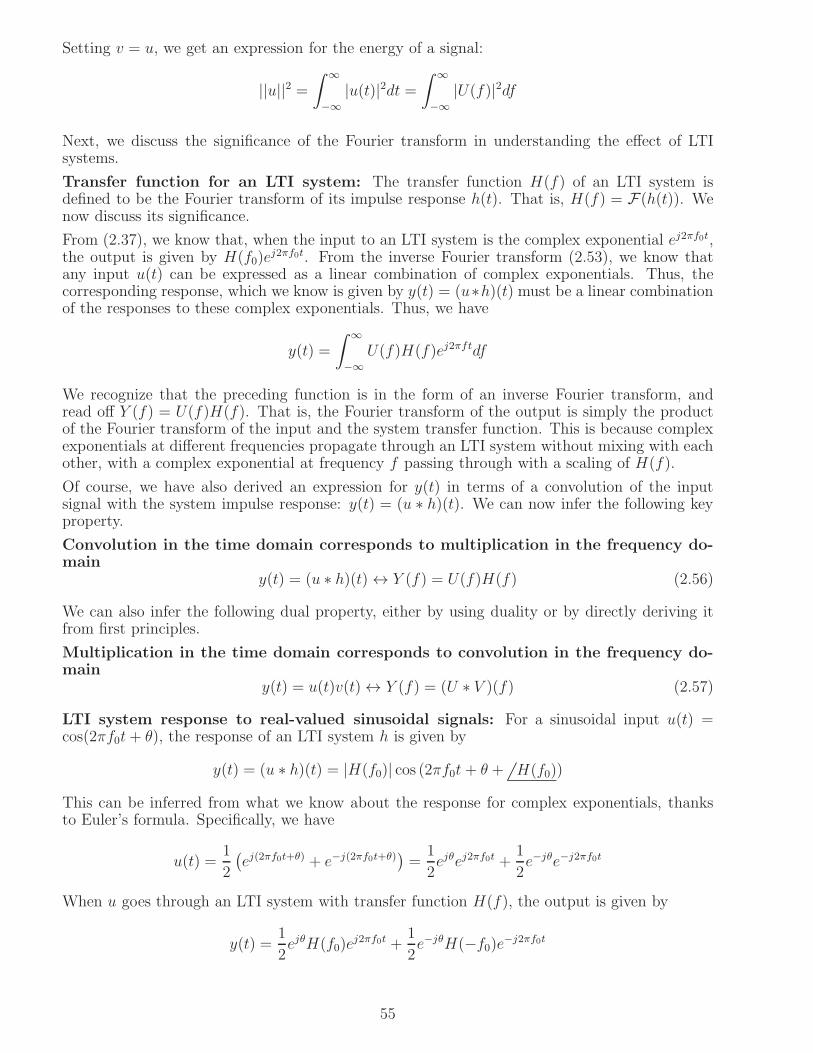
Setting v = u, we get an expression for the energy of a signal:

||u||2 =∫ ∞

−∞|u(t)|2dt =

∫ ∞

−∞|U(f)|2df

Next, we discuss the significance of the Fourier transform in understanding the effect of LTIsystems.

Transfer function for an LTI system: The transfer function H(f) of an LTI system isdefined to be the Fourier transform of its impulse response h(t). That is, H(f) = F(h(t)). Wenow discuss its significance.

From (2.37), we know that, when the input to an LTI system is the complex exponential ej2πf0t,the output is given by H(f0)e

j2πf0t. From the inverse Fourier transform (2.53), we know thatany input u(t) can be expressed as a linear combination of complex exponentials. Thus, thecorresponding response, which we know is given by y(t) = (u∗h)(t) must be a linear combinationof the responses to these complex exponentials. Thus, we have

y(t) =

∫ ∞

−∞U(f)H(f)ej2πftdf

We recognize that the preceding function is in the form of an inverse Fourier transform, andread off Y (f) = U(f)H(f). That is, the Fourier transform of the output is simply the productof the Fourier transform of the input and the system transfer function. This is because complexexponentials at different frequencies propagate through an LTI system without mixing with eachother, with a complex exponential at frequency f passing through with a scaling of H(f).

Of course, we have also derived an expression for y(t) in terms of a convolution of the inputsignal with the system impulse response: y(t) = (u ∗ h)(t). We can now infer the following keyproperty.

Convolution in the time domain corresponds to multiplication in the frequency do-main

y(t) = (u ∗ h)(t) ↔ Y (f) = U(f)H(f) (2.56)

We can also infer the following dual property, either by using duality or by directly deriving itfrom first principles.

Multiplication in the time domain corresponds to convolution in the frequency do-main

y(t) = u(t)v(t) ↔ Y (f) = (U ∗ V )(f) (2.57)

LTI system response to real-valued sinusoidal signals: For a sinusoidal input u(t) =cos(2πf0t+ θ), the response of an LTI system h is given by

y(t) = (u ∗ h)(t) = |H(f0)| cos (2πf0t + θ + H(f0))

This can be inferred from what we know about the response for complex exponentials, thanksto Euler’s formula. Specifically, we have

u(t) =1

2

(

ej(2πf0t+θ) + e−j(2πf0t+θ))

=1

2ejθej2πf0t +

1

2e−jθe−j2πf0t

When u goes through an LTI system with transfer function H(f), the output is given by

y(t) =1

2ejθH(f0)e

j2πf0t +1

2e−jθH(−f0)e−j2πf0t

55

If the system is physically realizable, the impulse response h(t) is real-valued, and the transferfunction is conjugate symmetric. Thus, if H(f0) = Gejφ (G ≥ 0), then H(−f0) = H∗(f0) =Ge−jφ. Substituting, we obtain

y(t) =G

2ej(2πf0t+θ+φ) +

G

2e−j(2πf0t+θ+φ) = G cos(2πf0t+ θ + φ)

This yields the well-known result that the sinusoid gets scaled by the magnitude of the transferfunction G = |H(f0)|, and gets phase shifted by the phase of the transfer function φ = H(f0).

Example 2.5.4 (Delay spread, coherence bandwidth, and fading for a multipathchannel) The transfer function of a multipath channel as in (2.36) is given by

H(f) = α1e−j2πfτ1 + ...+ αme

−j2πfτm (2.58)

Thus, the channel transfer function is a linear combination of complex exponentials in the fre-quency domain. As with any sinusoids, these can interfere constructively or destructively, leadingto significant fluctuations in H(f) as f varies. For wireless channels, this phenomenon is calledfrequency-selective fading. Let us examine the structure of the fading a little further. Suppose,without loss of generality, that the delays are in increasing order (i.e., τ1 < τ2 < ... < τm). Wecan then rewrite the transfer function as

H(f) = e−j2πfτ1

m∑

k=1

αke−j2πf(τk−τ1)

The first term e−j2πfτ1 corresponds simply to a pure delay τ1 (seen by all frequencies), and canbe dropped (taking τ1 as our time origin, without loss of generality), so that the transfer functioncan be rewritten as

H(f) = α1 +m∑

k=2

αke−j2πf(τk−τ1) (2.59)

The period of the kth sinusoid above (k ≥ 2) is 1/(τk − τ1), so that, the smallest period, andhence the fastest fluctuations as a function of f , occurs because of the largest delay differenceτd = τm − τ1, which we call the channel delay spread. Thus, for a frequency interval which issignificantly smaller than 1/τd, the variation of |H(f)| over the interval is small. We define thechannel coherence bandwidth as the inverse of the delay spread, i.e., as Bc = 1/(τm − τ1) =1/τd (this definition is not unique, but in general, the coherence bandwidth is defined to beinversely proportional to some appropriately defined measure of the channel delay spread). Aswe have noted, H(f) can be well modeled as constant over intervals significantly smaller thanthe coherence bandwidth.

Let us apply this to the example in Figure 2.14, where we have a multipath channel with impulseresponse h(t) = δ(t − 1) − 0.5δ(t − 1.5) + 0.5δ(t − 3.5). Dropping the first delay as before, wehave

H(f) = 1− 0.5e−jπf + 0.5e−j5πf

For concreteness, suppose that time is measured in microseconds (typical numbers for an outdoorwireless cellular link), so that frequency is measured in MHz. The delay spread is 2.5µs, hencethe coherence bandwidth is 400KHz. We therefore ballpark the size of the frequency intervalover which H(f) can be approximated as constant to about 40KHz (i.e., of size 10% of thecoherence bandwidth). Note that this is a very fuzzy estimate: if the larger delays occur withsmaller relative amplitudes, as is typical, then they have a smaller effect on H(f), and we couldpotentially approximate H(f) as constant over a larger fraction of the coherence bandwidth.Figure 2.22 depicts the fluctuations in H(f) first on a linear scale, and then on a log scale. A

56

plot of the transfer function magnitude is shown in Figure 2.22(a). This is the amplitude gain ona linear scale, and shows significant variations as a function of f (while we do not show it here,zooming in to 40 KHz bands shows relatively small fluctuations). The amount of fluctuationbecomes even more apparent on a log scale. Interpreting the gain at the smallest delay (α1 = 1in our case) as that of a nominal channel, the fading gain is defined as the power gain relativeto this nominal, and is given by 20 log10(|H(f)|/|α1|) in decibels (dB). This is shown in Figure2.22(b). Note that the fading gain can dip below -18 dB in our example, which we term a fadeof depth 18 dB. If we are using a “narrowband” signal which has a bandwidth small compared tothe coherence bandwidth, and happen to get hit by such a fade, then we can expect much poorerperformance than nominal. To combat this, one must use diversity. For example, a “wideband”signal whose bandwidth is larger than the coherence bandwidth provides frequency diversity,while, if we are constrained to use narrowband signals, we may need to introduce other forms ofdiversity (e.g., antenna diversity as in Software Lab 2.2).

−1 −0.8 −0.6 −0.4 −0.2 0 0.2 0.4 0.6 0.8 10

0.2

0.4

0.6

0.8

1

1.2

1.4

1.6

1.8

2

Frequency (MHz)

Mag

nitu

de o

f tra

nsfe

r fu

nctio

n

(a) Transfer Function Magnitude (linear scale)

−1 −0.8 −0.6 −0.4 −0.2 0 0.2 0.4 0.6 0.8 1−20

−15

−10

−5

0

5

10

Frequency (MHz)

Fad

ing

gain

(dB

)

(b) Frequency-selective fading (dB)

Figure 2.22: Multipath propagation causes severe frequency-selective fading.

2.5.2 Numerical computation using DFT

In many practical settings, we do not have nice analytical expressions for the Fourier or in-verse Fourier transforms, and must resort to numerical computation, typically using the discreteFourier transform (DFT). The DFT of a discrete time sequence u[n], n = 0, ..., N −1 of lengthN is given by

U [m] =N−1∑

n=0

u[n]e−j2πmn/N , m = 0, 1, ..., N − 1. (2.60)

Matlab is good at doing DFTs. When N is a power of 2, the DFT can be computed veryefficiently, and this procedure is called a Fast Fourier Transform (FFT). Comparing (2.60) withthe Fourier transform expression

U(f) =

∫ ∞

−∞u(t)e−j2πftdt (2.61)

we can view the sum in the DFT (2.60) as an approximation for the integral in (2.61) under theright set of conditions. Let us first assume that u(t) = 0 for t < 0: any waveform which can be

57

truncated so that most of its energy falls in a finite interval can be shifted so that this is true.Next, suppose that we sample the waveform with spacing ts to get

u[n] = u(nts)

Now, suppose we want to compute the Fourier transform U(f) for f = mfs, where fs is thedesired frequency resolution. We can approximate the integral for the Fourier transform by asum, using ts-spaced time samples as follows:

U(mfs) =

∫ ∞

−∞u(t)e−j2πmfstdt ≈

∑

n

u(nts)e−j2πmfsntsts

(dt in the integral is replaced by the sample spacing ts.) Since u[n] = u(nts), the approximationcan be computed using the DFT formula (2.60) as follows:

U(mfs) ≈ tsU [m] (2.62)

as long as fsts = 1N. That is, using a DFT of length N , we can get a frequency granularity of

fs =1

Nts. This implies that if we choose the time samples close together (in order to represent

u(t) accurately), then we must also use a large N to get a desired frequency granularity. Oftenthis means that we must pad the time domain samples with zeros.

Another important observation is that, while the DFT in (2.60) ranges from m = 0, ..., N − 1, itactually computes the Fourier transform for both positive and negative frequencies. Noting thatej2πmn/N = ej2π(−N+m)n/N , we realize that the DFT values for m = N/2, ..., N − 1 correspondto the Fourier transform evaluated at frequencies (m − N)fs = −N/2fs, ...,−fs. The DFTvalues for m = 0, ..., N/2 − 1 correspond to the Fourier transform evaluated at frequencies0, fs, ..., (N/2− 1)fs. Thus, we should swap the left and right halves of the DFT output in orderto represent positive and negative frequencies, with DC falling in the middle. Matlab actuallyhas a function, fftshift, that does this.

Note that the DFT (2.60) is periodic with period N , so that the Fourier transform approximation(2.62) is periodic with period Nfs =

1ts. We typically limit the range of frequencies over which

we use the DFT to compute the Fourier transform to the fundamental period (− 12ts, 12ts

). This is

consistent with the sampling theorem, which says that the sampling rate 1/ts must be at least aslarge as the size of the frequency band of interest. (The sampling theorem is reviewed in Chapter4, when we discuss digital modulation.)

Example 2.5.5 (DFT-based Fourier transform computation) Suppose that we want tocompute the Fourier transform of the sine pulse u(t) = sin πtI[0,1](t). The Fourier transform forthis can be computed analytically (see Problem 2.9) to be

U(f) =2 cosπf

π(1− 4f 2)e−jπf (2.63)

Note that U(f) has a 0/0 form at f = 1/2, but using L’Hospital’s rule, we can show thatU(1/2) 6= 0. Thus, the first zeros of U(f) are at f = ±3/2. This is a timelimited pulse andhence cannot be bandlimited, but U(f) decays as 1/f 2 for f large, so we can capture most ofthe energy of the pulse within a suitably chosen finite frequency interval. Let us use the DFT tocompute U(f) over f ∈ (−8, 8). This means that we set 1/(2ts) = 8, or ts = 1/16, which yieldsabout 16 samples over the interval [0, 1] over which the signal u(t) has support. Suppose nowthat we want the frequency granularity to be at least fs = 1/160. Then we must use a DFTwith N ≥ 1

tsfs= 2560 = Nmin. In order to efficiently compute the DFT using the FFT, we

choose N = 4096, the next power of 2 at least as large as Nmin. Code fragment 2.5.1 performsand plots this DFT. The resulting plot (with cosmetic touches not included in the code below)is displayed in Figure 2.23. It is useful to compare this with a plot obtained from the analyticalformula (2.63), and we leave that as an exercise.

58

−8 −6 −4 −2 0 2 4 6 80

0.1

0.2

0.3

0.4

0.5

0.6

0.7

Frequency

Mag

nitu

de S

pect

rum

Figure 2.23: Plot of magnitude spectrum of sine pulse in Example 2.5.5 obtained numericallyusing the DFT.

Code Fragment 2.5.1 Numerical computation of Fourier transform using FFT

ts=1/16; %sampling intervaltime_interval = 0:ts:1; %sampling time instants%%time domain signal evaluated at sampling instantssignal_timedomain = sin(pi*time_interval); %sinusoidal pulse in our examplefs_desired = 1/160; %desired frequency granularityNmin = ceil(1/(fs_desired*ts)); %minimum length DFT for desired frequency granularity%for efficient computation, choose FFT size to be power of 2Nfft = 2^(nextpow2(Nmin)) %FFT size = the next power of 2 at least as big as Nmin%Alternatively, one could also use DFT size equal to the minimum length%Nfft=Nmin;%note: fft function in Matlab is just the DFT when Nfft is not a power of 2%freq domain signal computed using DFT%fft function of size Nfft automatically zeropads as neededsignal_freqdomain = ts*fft(signal_timedomain,Nfft);%fftshift function shifts DC to center of spectrumsignal_freqdomain_centered = fftshift(signal_freqdomain);fs=1/(Nfft*ts); %actual frequency resolution attained%set of frequencies for which Fourier transform has been computed using DFTfreqs = ((1:Nfft)-1-Nfft/2)*fs;%plot the magnitude spectrumplot(freqs,abs(signal_freqdomain_centered));xlabel(’Frequency’);ylabel(’Magnitude Spectrum’);

2.6 Energy Spectral Density and Bandwidth

Communication channels have frequency-dependent characteristics, hence it is useful to appro-priately shape the frequency domain characteristics of the signals sent over them. Furthermore,for wireless communication systems, frequency spectrum is a particularly precious commodity,since wireless is a broadcast medium to be shared by multiple signals. It is therefore important

59

to quantify the frequency occupancy of communication signals. We provide a first exposure tothese concepts here via the notion of energy spectral density for finite energy signals. Theseideas are extended to finite power signals, for which we can define the analogous concept ofpower spectral density, in Chapter 4, “just in time” for our discussion of the spectral occupancyof digitally modulated signals. Once we know the energy or power spectral density of a signal,we shall see that there are a number of possible definitions of bandwidth, which is a measure ofthe size of the frequency interval occupied by the signal.

f*

∆

f∆uE ( )f*

H(f)

1Energy

Meteru(t)

f

Figure 2.24: Operational definition of energy spectral density.

Energy Spectral Density: The energy spectral density Eu(f) of a signal u(t) can be definedoperationally as shown in Figure 2.24. Pass the signal u(t) through an ideal narrowband filterwith transfer function as follows:

Hf∗(f) =

1, f ∗ − ∆f2< f < f ∗ + ∆f

2

0, else

The energy spectral density Eu(f∗) is defined to be the energy at the output of the filter, divided

by the width ∆f (in the limit as ∆f → 0). That is, the energy at the output of the filter isapproximately Eu(f

∗)∆f . But the Fourier transform of the filter output is

Y (f) = U(f)H(f) =

U(f), f ∗ − ∆f2< f < f ∗ + ∆f

2

0, else

By Parseval’s identity, the energy at the output of the filter is

∫ ∞

−∞|Y (f)|2 df =

∫ f∗+∆f2

f∗−∆f2

|U(f)|2 df ≈ |U(f ∗)|2 ∆f

assuming that U(f) varies smoothly and ∆f is small enough. We can now infer that the energyspectral density is simply the magnitude squared of the Fourier transform:

Eu(f) = |U(f)|2 (2.64)

The integral of the energy spectral density equals the signal energy, which is consistent withParseval’s identity.

The inverse Fourier transform of the energy spectral density has a nice intuitive interpretation.Noting that |U(f)|2 = U(f)U∗(f) and U∗(f) ↔ u∗(−t), let us define uMF (t) = u∗(−t) as (theimpulse response of) the matched filter for u(t), where the reasons for this term will be clarifiedlater. Then

|U(f)|2 = U(f)U∗(f) ↔ (u ∗ uMF )(τ) =∫

u(t)uMF (τ − t)dt=∫

u(t)u∗(t− τ)dt(2.65)

where t is a dummy variable for the integration, and the convolution is evaluated at the timevariable τ , which denotes the delay between the two versions of u being correlated: the extreme

60

right-hand side is simply the correlation of u with itself (after complex conjugation), evaluatedat different delays τ . We call this the autocorrelation function of the signal u. We have thereforeshown the following.

For a finite energy signal, the energy spectral density and the autocorrelation function form aFourier transform pair.

Bandwidth: The bandwidth of a signal u(t) is loosely defined to be the size of the bandof frequencies occupied by U(f). The definition is “loose” because the concept of occupancycan vary, depending on the application, since signals are seldom strictly bandlimited. Onepossibility is to consider the band over which |U(f)|2 is within some fraction of its peak value(setting the fraction equal to 1

2corresponds to the 3 dB bandwidth). Alternatively, we might

be interested in energy containment bandwidth, which is the size of the smallest band whichcontains a specified fraction of the signal energy (for a finite power signal, we define analogouslythe power containment bandwidth).

Only positive frequencies count when computing bandwidth for physical (real-valued)signals: For physically realizable (i.e., real-valued) signals, bandwidth is defined as its occupancyof positive frequencies, because conjugate symmetry implies that the information at negative fre-quencies is redundant.

While physically realizable time domain signals are real-valued, we shall soon introduce complex-valued signals that have useful physical interpretation, in the sense that they have a well-definedmapping to physically realizable signals. Conjugate symmetry in the frequency domain does nothold for complex-valued time domain signals, with different information contained in positiveand negative frequencies in general. Thus, the bandwidth for a complex-valued signal is definedas the size of the frequency band it occupies over both positive and negative frequencies. Thejustification for this convention becomes apparent later in this chapter.

Example 2.6.1 Some bandwidth computations(a) Consider u(t) = sinc(2t), where the unit of time is microseconds. Then the unit of frequencyis MHz, and U(f) = 1

2I[−1,1](f) is strictly bandlimited with 2 MHz.

(b) Now, consider the timelimited waveform u(t) = I[2,4](t), where the unit of time is microsec-onds. Then U(f) = 2sinc(2f)e−j6πf , which is not bandlimited. The 99% energy containmentbandwidth W is defined by the equation

∫ W

−W

|U(f)|2df = 0.99

∫ ∞

−∞|U(f)|2df = 0.99

∫ ∞

−∞|u(t)|2dt = 0.99

∫ 4

2

12dt = 1.98

where we use Parseval’s identity to simplify computation for timelimited waveforms. Using thefact that |U(f)| is even, we obtain that

1.98 = 2

∫ W

0

|U(f)|2df = 2

∫ W

0

4sinc2(2f)df

We can now solve numerically to obtain W ≈ 5.1 MHz.

2.7 Baseband and Passband Signals

Baseband: A signal u(t) is said to be baseband if the signal energy is concentrated in a bandaround DC, and

U(f) ≈ 0, |f | > W (2.66)

for some W > 0. Similarly, a channel modeled as a linear time invariant system is said to bebaseband if its transfer function H(f) has support concentrated around DC, and satisfies (2.66).

61

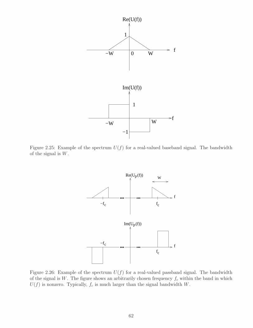
Im(U(f))

f0

1

Re(U(f))

f

1

−1

−W W

−W W

Figure 2.25: Example of the spectrum U(f) for a real-valued baseband signal. The bandwidthof the signal is W .

Re(U (f))

fc

−fc

−fc

fc

f

p

f

p

W

Im(U (f))

Figure 2.26: Example of the spectrum U(f) for a real-valued passband signal. The bandwidthof the signal is W . The figure shows an arbitrarily chosen frequency fc within the band in whichU(f) is nonzero. Typically, fc is much larger than the signal bandwidth W .

62

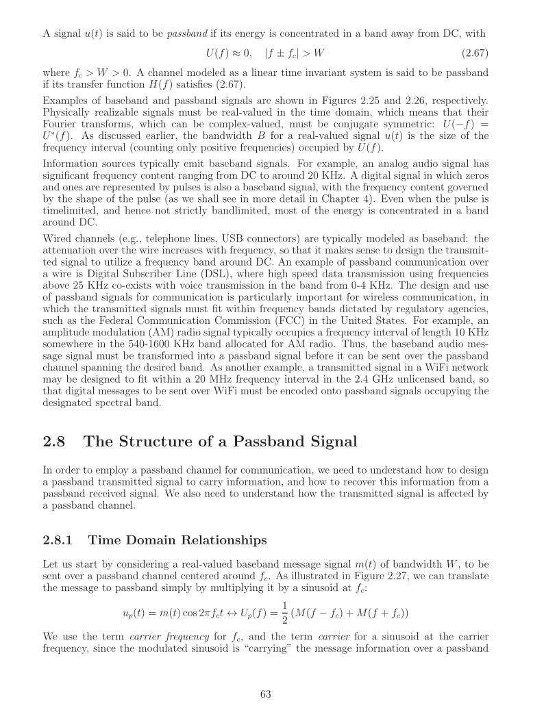
A signal u(t) is said to be passband if its energy is concentrated in a band away from DC, with

U(f) ≈ 0, |f ± fc| > W (2.67)

where fc > W > 0. A channel modeled as a linear time invariant system is said to be passbandif its transfer function H(f) satisfies (2.67).

Examples of baseband and passband signals are shown in Figures 2.25 and 2.26, respectively.Physically realizable signals must be real-valued in the time domain, which means that theirFourier transforms, which can be complex-valued, must be conjugate symmetric: U(−f) =U∗(f). As discussed earlier, the bandwidth B for a real-valued signal u(t) is the size of thefrequency interval (counting only positive frequencies) occupied by U(f).

Information sources typically emit baseband signals. For example, an analog audio signal hassignificant frequency content ranging from DC to around 20 KHz. A digital signal in which zerosand ones are represented by pulses is also a baseband signal, with the frequency content governedby the shape of the pulse (as we shall see in more detail in Chapter 4). Even when the pulse istimelimited, and hence not strictly bandlimited, most of the energy is concentrated in a bandaround DC.

Wired channels (e.g., telephone lines, USB connectors) are typically modeled as baseband: theattenuation over the wire increases with frequency, so that it makes sense to design the transmit-ted signal to utilize a frequency band around DC. An example of passband communication overa wire is Digital Subscriber Line (DSL), where high speed data transmission using frequenciesabove 25 KHz co-exists with voice transmission in the band from 0-4 KHz. The design and useof passband signals for communication is particularly important for wireless communication, inwhich the transmitted signals must fit within frequency bands dictated by regulatory agencies,such as the Federal Communication Commission (FCC) in the United States. For example, anamplitude modulation (AM) radio signal typically occupies a frequency interval of length 10 KHzsomewhere in the 540-1600 KHz band allocated for AM radio. Thus, the baseband audio mes-sage signal must be transformed into a passband signal before it can be sent over the passbandchannel spanning the desired band. As another example, a transmitted signal in a WiFi networkmay be designed to fit within a 20 MHz frequency interval in the 2.4 GHz unlicensed band, sothat digital messages to be sent over WiFi must be encoded onto passband signals occupying thedesignated spectral band.

2.8 The Structure of a Passband Signal

In order to employ a passband channel for communication, we need to understand how to designa passband transmitted signal to carry information, and how to recover this information from apassband received signal. We also need to understand how the transmitted signal is affected bya passband channel.

2.8.1 Time Domain Relationships

Let us start by considering a real-valued baseband message signal m(t) of bandwidth W , to besent over a passband channel centered around fc. As illustrated in Figure 2.27, we can translatethe message to passband simply by multiplying it by a sinusoid at fc:

up(t) = m(t) cos 2πfct↔ Up(f) =1

2(M(f − fc) +M(f + fc))

We use the term carrier frequency for fc, and the term carrier for a sinusoid at the carrierfrequency, since the modulated sinusoid is “carrying” the message information over a passband

63

Baseband

f c−fc f cf

0−W

|M(f))|

W f−W

|U(f)|,|V(f)|Modulation

Passband

Figure 2.27: A baseband message of bandwidth W is translated to passband by multiplying bya sinusoid at frequency fc, as long as fc > W .

channel. Instead of a cosine, we could also use a sine:

vp(t) = m(t) sin 2πfct↔ Vp(f) =1

2j(M(f − fc)−M(f + fc))

Note that |Up(f)| and |Vp(f)| have frequency content in a band around fc, and are passbandsignals (i.e., living in a band not containing DC) as long as fc > W .

I and Q components: If we use both the cosine and sine carriers, we can construct a passbandsignal of the form

up(t) = uc(t) cos 2πfct− us(t) sin 2πfct (2.68)

where uc and us are real baseband signals of bandwidth at most W , with fc > W . The signaluc(t) is called the in-phase (or I) component, and us(t) is called the quadrature (or Q) component.The negative sign for the Q term is a standard convention. Since the sinusoidal terms are entirelypredictable once we specify fc, all information in the passband signal up must be contained inthe I and Q components. Modulation for a passband channel therefore corresponds to choosinga method of encoding information into the I and Q components of the transmitted signal, whiledemodulation corresponds to extracting this information from the received passband signal. Inorder to accomplish modulation and demodulation, we must be able to upconvert from basebandto passband, and downconvert from passband to baseband, as follows.

cos 2 f t

LowpassFilter

LowpassFilter

cu (t)

su (t)

pu (t)

su (t)

cu (t)

pu (t)

π2cos 2 f tc

−sin 2 f tπ c π−2sin 2 f tc

(baseband to passband)Upconversion Downconversion

(passband to baseband)

π c

Figure 2.28: Upconversion from baseband to passband, and downconversion from passband tobaseband.

Upconversion and downconversion: Equation (2.68) immediately tells us how to upconvertfrom baseband to passband. To downconvert from passband to baseband, consider

2up(t) cos(2πfct) = 2uc(t) cos2 2πfct− 2us(t) sin 2πfct cos 2πfct

= uc(t) + uc(t) cos 4πfct− us(t) sin 4πfct

64

The first term on the extreme right-hand side is the I component uc(t), a baseband signal. Thesecond and third terms are passband signals at 2fc, which we can get rid of by lowpass filtering.Similarly, we can obtain the Q component us(t) by lowpass filtering −2up(t) sin 2πfct. Blockdiagrams for upconversion and downconversion are depicted in Figure 2.28. Implementation ofthese operations could, in practice, be done in multiple stages, and requires careful analog circuitdesign.

We now dig deeper into the structure of a passband signal. First, can we choose the I and Qcomponents freely, independent of each other? The answer is yes: the I and Q componentsprovide two parallel, orthogonal “channels” for encoding information, as we show next.

Orthogonality of I and Q channels: The passband waveform ap(t) = uc(t) cos 2πfct corre-sponding to the I component, and the passband waveform bp(t) = us(t) sin 2πfct correspondingto the Q component, are orthogonal. That is,

〈ap, bp〉 = 0 (2.69)

Let

x(t) = ap(t)bp(t) = uc(t)us(t) cos 2πfct sin 2πfct =1

2uc(t)us(t) sin 4πfct

We prove the desired result by showing that x(t) is a passband signal at 2fc, so that its DCcomponent is zero. That is,

∫ ∞

−∞x(t)dt = X(0) = 0

which is the desired result. To show this, note that

p(t) =1

2uc(t)us(t) ↔

1

2(Uc ∗ Us)(f)

is a baseband signal: if Uc(f) is baseband with bandwidth W1 and Us(f) is baseband withbandwidth W2, then their convolution has bandwidth at most W1 +W2. In order for ap to bepassband, we must have fc > W1, and in order for bp to be passband, we must have fc > W2.Thus, 2fc > W1 +W2, which means that x(t) = p(t) sin 4πfct is passband around 2fc, and istherefore zero at DC. This completes the derivation.

Example 2.8.1 (Passband signal): The signal

up(t) = I[0,1](t) cos 300πt− (1− |t|)I[−1,1](t) sin 300πt

is a passband signal with I component uc(t) = I[0,1](t) and Q component us(t) = (1−|t|)I[−1,1](t).This example illustrates that we do not require strict bandwidth limitations in our definitionsof passband and baseband: the I and Q components are timelimited, and hence cannot bebandlimited. However, they are termed baseband signals because most of their energy lies inbaseband. Similarly, up(t) is termed a passband signal, since most of its frequency content liesin a small band around 150 Hz.

Envelope and phase: Since a passband signal up is equivalent to a pair of real-valued basebandwaveforms (uc, us), passband modulation is often called two-dimensional modulation. The repre-sentation (2.68) in terms of I and Q components corresponds to thinking of this two-dimensionalwaveform in rectangular coordinates (the “cosine axis” and the “sine axis”). We can also rep-resent the passband waveform using polar coordinates. Consider the rectangular-polar transfor-mation

e(t) =√

u2c(t) + u2s(t) , θ(t) = tan−1 us(t)

uc(t)

65

where e(t) ≥ 0 is termed the envelope and θ(t) is the phase. This corresponds to uc(t) =e(t) cos θ(t) and us(t) = e(t) sin θ(t). Substituting in (2.68), we obtain

up(t) = e(t) cos θ(t) cos 2πfct− e(t) sin θ(t) sin 2πfct = e(t) cos (2πfct+ θ(t)) (2.70)

This provides an alternate representation of the passband signal in terms of baseband envelopeand phase signals.

u(t)s

u (t)c

I

Q

θ( )te(t)

u (t)

Figure 2.29: Geometry of the complex envelope.

Complex envelope: To obtain a third representation of a passband signal, we note that atwo-dimensional point can also be mapped to a complex number; see Section 2.1. We define thecomplex envelope u(t) of the passband signal up(t) in (2.68) and (2.70) as follows:

u(t) = uc(t) + jus(t) = e(t)ejθ(t) (2.71)

We can now express the passband signal in terms of its complex envelope. From (2.70), we seethat

up(t) = e(t)Re(

ej(2πfct+θ(t)))

= Re(

e(t)ej(2πfct+θ(t)))

= Re(

e(t)ejθ(t)ej2πfct)

This leads to our third representation of a passband signal:

up(t) = Re(

u(t)ej2πfct)

(2.72)

While we have obtained (2.72) using the polar representation (2.70), we should also check thatit is consistent with the rectangular representation (2.68), writing out the real and imaginaryparts of the complex waveforms above as follows:

u(t)ej2πfct = (uc(t) + jus(t)) (cos 2πfct+ j sin 2πfct)= (uc(t) cos 2πfct− us(t) sin 2πfct) + j (us(t) cos 2πfct+ uc(t) sin 2πfct)

(2.73)

Taking the real part, we obtain the expression (2.68) for up(t).

The relationship between the three time domain representations of a passband signal in termsof its complex envelope is depicted in Figure 2.29. We now specify the corresponding frequencydomain relationship.

Information resides in complex baseband: The complex baseband representation corre-sponds to subtracting out the rapid, but predictable, phase variation due to the fixed reference

66

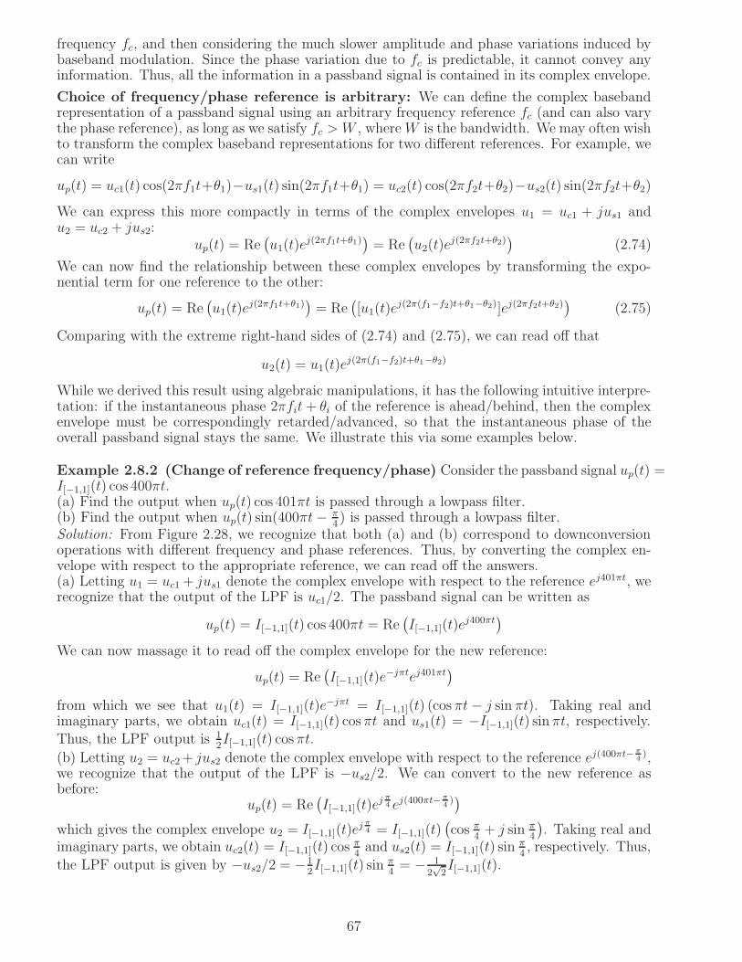
frequency fc, and then considering the much slower amplitude and phase variations induced bybaseband modulation. Since the phase variation due to fc is predictable, it cannot convey anyinformation. Thus, all the information in a passband signal is contained in its complex envelope.

Choice of frequency/phase reference is arbitrary: We can define the complex basebandrepresentation of a passband signal using an arbitrary frequency reference fc (and can also varythe phase reference), as long as we satisfy fc > W , whereW is the bandwidth. We may often wishto transform the complex baseband representations for two different references. For example, wecan write

up(t) = uc1(t) cos(2πf1t+θ1)−us1(t) sin(2πf1t+θ1) = uc2(t) cos(2πf2t+θ2)−us2(t) sin(2πf2t+θ2)We can express this more compactly in terms of the complex envelopes u1 = uc1 + jus1 andu2 = uc2 + jus2:

up(t) = Re(

u1(t)ej(2πf1t+θ1)

)

= Re(

u2(t)ej(2πf2t+θ2)

)

(2.74)

We can now find the relationship between these complex envelopes by transforming the expo-nential term for one reference to the other:

up(t) = Re(

u1(t)ej(2πf1t+θ1)

)

= Re(

[u1(t)ej(2π(f1−f2)t+θ1−θ2)]ej(2πf2t+θ2)

)

(2.75)

Comparing with the extreme right-hand sides of (2.74) and (2.75), we can read off that

u2(t) = u1(t)ej(2π(f1−f2)t+θ1−θ2)

While we derived this result using algebraic manipulations, it has the following intuitive interpre-tation: if the instantaneous phase 2πfit+ θi of the reference is ahead/behind, then the complexenvelope must be correspondingly retarded/advanced, so that the instantaneous phase of theoverall passband signal stays the same. We illustrate this via some examples below.

Example 2.8.2 (Change of reference frequency/phase) Consider the passband signal up(t) =I[−1,1](t) cos 400πt.(a) Find the output when up(t) cos 401πt is passed through a lowpass filter.(b) Find the output when up(t) sin(400πt− π

4) is passed through a lowpass filter.

Solution: From Figure 2.28, we recognize that both (a) and (b) correspond to downconversionoperations with different frequency and phase references. Thus, by converting the complex en-velope with respect to the appropriate reference, we can read off the answers.(a) Letting u1 = uc1+ jus1 denote the complex envelope with respect to the reference ej401πt, werecognize that the output of the LPF is uc1/2. The passband signal can be written as

up(t) = I[−1,1](t) cos 400πt = Re(

I[−1,1](t)ej400πt

)

We can now massage it to read off the complex envelope for the new reference:

up(t) = Re(

I[−1,1](t)e−jπtej401πt

)

from which we see that u1(t) = I[−1,1](t)e−jπt = I[−1,1](t) (cos πt− j sin πt). Taking real and

imaginary parts, we obtain uc1(t) = I[−1,1](t) cosπt and us1(t) = −I[−1,1](t) sin πt, respectively.Thus, the LPF output is 1

2I[−1,1](t) cosπt.

(b) Letting u2 = uc2+ jus2 denote the complex envelope with respect to the reference ej(400πt−π4),

we recognize that the output of the LPF is −us2/2. We can convert to the new reference asbefore:

up(t) = Re(

I[−1,1](t)ej π4 ej(400πt−

π4))

which gives the complex envelope u2 = I[−1,1](t)ej π4 = I[−1,1](t)

(

cos π4+ j sin π

4

)

. Taking real andimaginary parts, we obtain uc2(t) = I[−1,1](t) cos

π4and us2(t) = I[−1,1](t) sin

π4, respectively. Thus,

the LPF output is given by −us2/2 = −12I[−1,1](t) sin

π4= − 1

2√2I[−1,1](t).

67

From a practical point of view, keeping track of frequency/phase references becomes importantfor the task of synchronization. For example, the carrier frequency used by the transmitter forupconversion may not be exactly equal to that used by the receiver for downconversion. Thus,the receiver must compensate for the phase rotation incurred by the complex envelope at theoutput of the downconverter, as illustrated by the following example.

Example 2.8.3 (Modeling and compensating for frequency/phase offsets in complexbaseband): Consider the passband signal up (2.68), with complex baseband representationu = uc + jus. Now, consider a phase-shifted version of the passband signal

up(t) = uc(t) cos(2πfct+ θ(t))− us(t) sin(2πfct + θ(t))

where θ(t) may vary slowly with time. For example, a carrier frequency offset ∆f and a phaseoffset γ corresponds to θ(t) = 2π∆ft + γ. Suppose, now, that the signal is downconverted asin Figure 2.28, where we take the phase reference as that of the receiver’s local oscillator (LO).How do the I and Q components depend on the phase offset of the received signal relative to theLO? The easiest way to answer this is to find the complex envelope of up with respect to fc. Todo this, we write up in the standard form (2.70) as follows:

up(t) = Re(

u(t)ej(2πfct+θ(t)))

Comparing with the desired form

up(t) = Re(u(t)ej2πfct)

we can read offu(t) = u(t)ejθ(t) (2.76)

Equation (2.76) relates the complex envelopes before and after a phase offset. We can expandout this “polar form” representation to obtain the corresponding relationship between the I andQ components. Suppressing time dependence from the notation, we can rewrite (2.76) as

uc + jus = (uc + jus)(cos θ + j sin θ)

using Euler’s formula. Equating real and imaginary parts on both sides, we obtain

uc = uc cos θ − us sin θus = uc sin θ + us cos θ

(2.77)

The phase offset therefore results in the I and Q components being mixed together at the outputof the downconverter. Thus, for a coherent receiver recovers the original I and Q components uc,us, we must account for the (possibly time varying) phase offset θ(t). In particular, if we havean estimate of the phase offset, then we can undo it by inverting the relationship in (2.76):

u(t) = u(t)e−jθ(t) (2.78)

which can be written out in terms of real-valued operations as follows:

uc = uc cos θ + us sin θus = −uc sin θ + us cos θ

(2.79)

The preceding computations provide a typical example of the advantage of working in complexbaseband. Relationships between passband signals can be compactly represented in complexbaseband, as in (2.76) and (2.78). For signal processing using real-valued arithmetic, thesecomplex baseband relationships can be expanded out to obtain relationships involving real-valuedquantities, as in (2.77) and (2.79). See Software Lab 2.1 for an example of such computations.

68

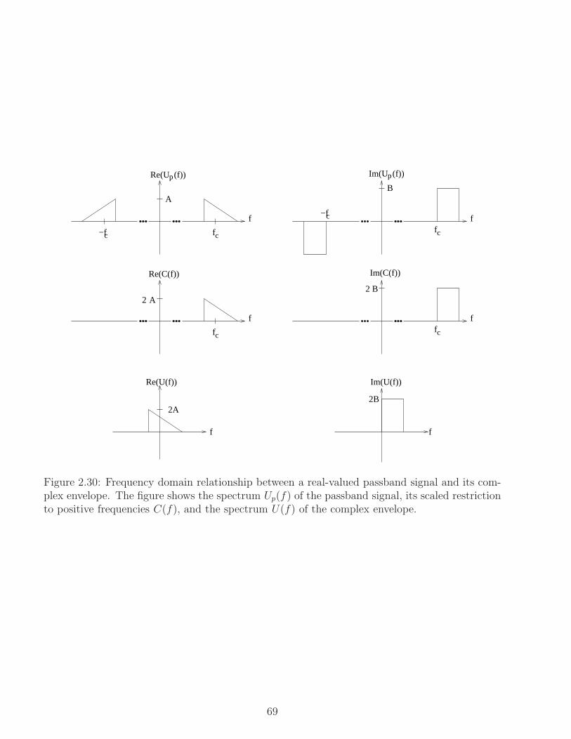
Im(U (f))

fcfc

fc−fc

−fc

fc

f f

f

p

f

p

AB

f f

A2B2

Re(C(f)) Im(C(f))

2A2B

Re(U(f)) Im(U(f))

Re(U (f))

Figure 2.30: Frequency domain relationship between a real-valued passband signal and its com-plex envelope. The figure shows the spectrum Up(f) of the passband signal, its scaled restrictionto positive frequencies C(f), and the spectrum U(f) of the complex envelope.

69

2.8.2 Frequency Domain Relationships

Consider an arbitrary complex-valued baseband waveform u(t) whose frequency content is con-tained in [−W,W ], and suppose that fc > W . We want to show that

up(t) = Re(

u(t)ej2πfct)

= Re (c(t)) (2.80)

is a real-valued passband signal whose frequency is concentrated around ±fc, away from DC. Let

c(t) = u(t)ej2πfct ↔ C(f) = U(f − fc) (2.81)

That is, C(f) is the complex envelope U(f), shifted to the right by fc. Since U(f) has frequencycontent in [−W,W ], C(f) has frequency content around [fc−W, fc+W ]. Since fc−W > 0, thisband does not include DC. Now,

up(t) = Re (c(t)) =1

2(c(t) + c∗(t)) ↔ Up(f) =

1

2(C(f) + C∗(−f))

Since C∗(−f) is the complex conjugated version of C(f), flipped around the origin, it has fre-quency content in the band of negative frequencies [−fc −W,−fc +W ] around −fc, which doesnot include DC because −fc +W < 0. Thus, we have shown that up(t) is a passband signal. Itis real-valued by virtue of its construction using the time domain equation (2.80), which involvestaking the real part. But we can also doublecheck for consistency in the frequency domain:Up(f) is conjugate symmetric, since its positive frequency component is C(f), and its nega-tive frequency component is C∗(−f). Substituting C(f) by U(f − fc), we obtain the passbandspectrum in terms of the complex baseband spectrum:

Up(f) =1

2(U(f − fc) + U∗(−f − fc)) (2.82)

So far, we have seen how to construct a real-valued passband signal given a complex-valuedbaseband signal. To go in reverse, we must answer the following: do the equivalent representa-tions (2.68), (2.70), (2.72) and (2.82) hold for any passband signal, and if so, how do we findthe spectrum of the complex envelope given the spectrum of the passband signal? To answerthese questions, we simply trace back the steps we used to arrive at (2.82). Given the spec-trum Up(f) for a real-valued passband signal up(t), we construct C(f) as a scaled version ofU+p (f) = Up(f)I[0,∞)(f), the positive frequency part of Up(f), as follows:

C(f) = 2U+p (f) =

2Up(f) , f > 00 , f < 0

This means that Up(f) =12C(f) for positive frequencies. By the conjugate symmetry of Up(f),

the negative frequency component must be 12C∗(−f), so that Up(f) =

12C(f) + 1

2C∗(−f). In the

time domain, this corresponds to

up(t) =1

2c(t) +

1

2c∗(t) = Re (c(t)) (2.83)

Now, let us define the complex envelope as follows:

u(t) = c(t)e−j2πfct ↔ U(f) = C(f + fc)

Since c(t) = u(t)ej2πfct, we obtain the desired relationship (2.68) on substituting into (2.83).Since C(f) has frequency content in a band around fc, U(f), which is obtained by shifting C(f)to the left by fc, is indeed a baseband signal with frequency content in a band around DC.

70

Frequency domain expressions for I and Q components: If we are given the time domaincomplex envelope, we can read off the I and Q components as the real and imaginary parts:

uc(t) = Re(u(t)) = 12(u(t) + u∗(t))

us(t) = Im(u(t)) = 12j(u(t)− u∗(t))

Taking Fourier transforms, we obtain

Uc(f) =12(U(f) + U∗(−f))

Us(f) =12j(U(f)− U∗(−f))

Figure 2.30 shows the relation between the passband signal Up(f), its scaled version C(f) re-stricted to positive frequencies, and the complex baseband signal U(f). As this example em-phasizes, all of these spectra can, in general, be complex-valued. Equation (2.80) corresponds tostarting with an arbitrary baseband signal U(f) as in the bottom of the figure, and constructingC(f) as depicted in the middle of the figure. We then use C(f) to construct a conjugate sym-metric passband signal Up(f), proceeding from the middle of the figure to the top. This examplealso shows that U(f) does not, in general, obey conjugate symmetry, so that the baseband signalu(t) is, in general, complex-valued. However, by construction, Up(f) is conjugate symmetric, andhence the passband signal up(t) is real-valued.

Example 2.8.4 Let vp(t) denote a real-valued passband signal, with Fourier transform Vp(f)specified as follows for negative frequencies:

Vp(f) =

−(f + 99) −101 ≤ f ≤ −990 f < −101 or − 99 < f ≤ 0

(a) Sketch Vp(f) for both positive and negative frequencies.(b) Without explicitly taking the inverse Fourier transform, can you say whether vp(t) = vp(−t)or not?(c) Find and sketch Vc(f) and Vs(f), the Fourier transforms of the I and Q components withrespect to a reference frequency fc = 99. Do this without going to the time domain.(d) Find an explicit time domain expression for the output when vp(t) cos 200πt is passed throughan ideal lowpass filter of bandwidth 4.(e) Find an explicit time domain expression for the output when vp(t) sin 202πt is passed throughan ideal lowpass filter of bandwidth 4.Solution:

f

p

~ ~~ ~

−101 −99 99 101

2

V (f)

Figure 2.31: Sketch of passband spectrum for Example 2.8.4.

(a) Since vp(t) is real-valued, we have Vp (f) = V ∗p (−f). Since the spectrum is also given to be

real-valued for f ≤ 0, we have V ∗p (−f) = Vp (−f). The spectrum is sketched in Figure 2.31.

(b) Yes, vp(t) = vp(−t). Since vp(t) is real-valued, we have vp(−t) = v∗p(−t) ↔ V ∗p (f). But

V ∗p (f) = Vp(f), since the spectrum is real-valued.

71

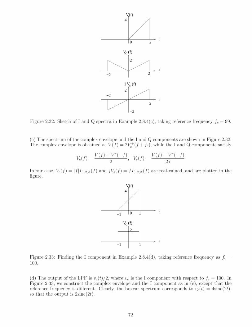
−2

f20

4V(f)

V (f)c

f2−2

2

j V (f)s

f2

−22

Figure 2.32: Sketch of I and Q spectra in Example 2.8.4(c), taking reference frequency fc = 99.

(c) The spectrum of the complex envelope and the I and Q components are shown in Figure 2.32.The complex envelope is obtained as V (f) = 2V +

p (f + fc), while the I and Q components satisfy

Vc(f) =V (f) + V ∗(−f)

2, Vs(f) =

V (f)− V ∗(−f)2j

In our case, Vc(f) = |f |I[−2,2](f) and jVs(f) = fI[−2,2](f) are real-valued, and are plotted in thefigure.

2

c

f0

4V(f)

f

−1 1

−1 1

V (f)

Figure 2.33: Finding the I component in Example 2.8.4(d), taking reference frequency as fc =100.

(d) The output of the LPF is vc(t)/2, where vc is the I component with respect to fc = 100. InFigure 2.33, we construct the complex envelope and the I component as in (c), except that thereference frequency is different. Clearly, the boxcar spectrum corresponds to vc(t) = 4sinc(2t),so that the output is 2sinc(2t).

72

−2

s

f20

V(f)4

f

2

2

−2

j V (f)

Figure 2.34: Finding the Q component in Example 2.8.4(e), taking reference frequency as fc =101.

(e) The output of the LPF is −vs(t)/2, where vs is the I component with respect to fc = 101. InFigure 2.34, we construct the complex envelope and the Q component as in (c), except that thereference frequency is different. We now have to take the inverse Fourier transform, which is alittle painful if we do it from scratch. Instead, let us differentiate to see that

jdVs(f)

df= I[−2,2](f)− 4δ(f) ↔ 4sinc(4t)− 4

But dVs(f)df

↔ −j2πtvs(t), so that j dVs(f)df

↔ 2πtvs(t). We therefore obtain that 2πtvs(t) =

4sinc(4t)− 4, or vs(t) =2(sinc(4t)−1)

πt. Thus, the output of the LPF is −vs(t)/2, or (1−sinc(4t))

πt.

U(f)

p

Y (f)p

fc

fc

fc

pU (f)

f

f

f f

f

f

H(f)

A

B

AB

Y(f)

Complex BasebandPassband

Output

Input

Filter2A

2AB

2B

H (f)

Figure 2.35: The relationship between passband filtering and its complex baseband analogue.

73

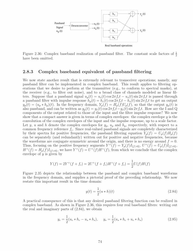
Real baseband operations

c

hs

hc

hs

cy (t)

y (t)spu (t)

cu (t)

su (t)

−

Signal

Passband Downconverter

h

Figure 2.36: Complex baseband realization of passband filter. The constant scale factors of 12

have been omitted.

2.8.3 Complex baseband equivalent of passband filtering

We now state another result that is extremely relevant to transceiver operations; namely, anypassband filter can be implemented in complex baseband. This result applies to filtering op-erations that we desire to perform at the transmitter (e.g., to conform to spectral masks), atthe receiver (e.g., to filter out noise), and to a broad class of channels modeled as linear fil-ters. Suppose that a passband signal up(t) = uc(t) cos 2πfct − us(t) sin 2πfct is passed througha passband filter with impulse response hp(t) = hc(t) cos 2πfct− hs(t) sin 2πfct to get an outputyp(t) = (up ∗ hp)(t). In the frequency domain, Yp(f) = Hp(f)Up(f), so that the output yp(t) isalso passband, and can be written as yp(t) = yc(t) cos 2πfct−ys(t) sin 2πfct. How are the I and Qcomponents of the output related to those of the input and the filter impulse response? We nowshow that a compact answer is given in terms of complex envelopes: the complex envelope y is theconvolution of the complex envelopes of the input and the impulse response, up to a scale factor.Let y, u and h denote the complex envelopes for yp, up and hp, respectively, with respect to acommon frequency reference fc. Since real-valued passband signals are completely characterizedby their spectra for positive frequencies, the passband filtering equation Yp(f) = Up(f)Hp(f)can be separately (and redundantly) written out for positive and negative frequencies, becausethe waveforms are conjugate symmetric around the origin, and there is no energy around f = 0.Thus, focusing on the positive frequency segments Y +(f) = Yp(f)If>0, U

+(f) = Up(f)If>0,H+(f) = Hp(f)If>0, we have Y

+(f) = U+(f)H+(f), from which we conclude that the complexenvelope of y is given by

Y (f) = 2Y +(f + fc) = 2U+(f + fc)H+(f + fc) =

1

2U(f)H(f)

Figure 2.35 depicts the relationship between the passband and complex baseband waveformsin the frequency domain, and supplies a pictorial proof of the preceding relationship. We nowrestate this important result in the time domain:

y(t) =1

2(u ∗ h)(t) (2.84)

A practical consequence of this is that any desired passband filtering function can be realized incomplex baseband. As shown in Figure 2.36, this requires four real baseband filters: writing outthe real and imaginary parts of (2.84), we obtain

yc =1

2(uc ∗ hc − us ∗ hs), ys =

1

2(us ∗ hc + uc ∗ hs) (2.85)

74

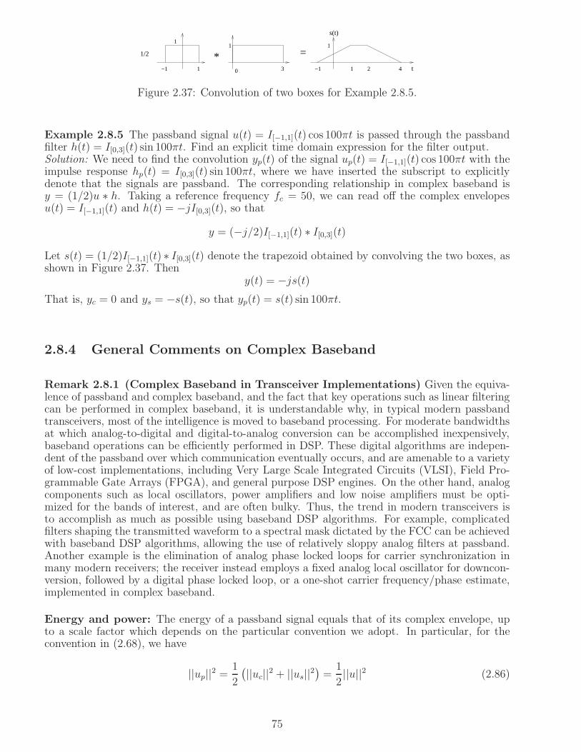
t−1 1 0 3

11

−1 1 2 4

1

1/2 * =

s(t)

Figure 2.37: Convolution of two boxes for Example 2.8.5.

Example 2.8.5 The passband signal u(t) = I[−1,1](t) cos 100πt is passed through the passbandfilter h(t) = I[0,3](t) sin 100πt. Find an explicit time domain expression for the filter output.Solution: We need to find the convolution yp(t) of the signal up(t) = I[−1,1](t) cos 100πt with theimpulse response hp(t) = I[0,3](t) sin 100πt, where we have inserted the subscript to explicitlydenote that the signals are passband. The corresponding relationship in complex baseband isy = (1/2)u ∗ h. Taking a reference frequency fc = 50, we can read off the complex envelopesu(t) = I[−1,1](t) and h(t) = −jI[0,3](t), so that

y = (−j/2)I[−1,1](t) ∗ I[0,3](t)

Let s(t) = (1/2)I[−1,1](t) ∗ I[0,3](t) denote the trapezoid obtained by convolving the two boxes, asshown in Figure 2.37. Then

y(t) = −js(t)That is, yc = 0 and ys = −s(t), so that yp(t) = s(t) sin 100πt.

2.8.4 General Comments on Complex Baseband

Remark 2.8.1 (Complex Baseband in Transceiver Implementations) Given the equiva-lence of passband and complex baseband, and the fact that key operations such as linear filteringcan be performed in complex baseband, it is understandable why, in typical modern passbandtransceivers, most of the intelligence is moved to baseband processing. For moderate bandwidthsat which analog-to-digital and digital-to-analog conversion can be accomplished inexpensively,baseband operations can be efficiently performed in DSP. These digital algorithms are indepen-dent of the passband over which communication eventually occurs, and are amenable to a varietyof low-cost implementations, including Very Large Scale Integrated Circuits (VLSI), Field Pro-grammable Gate Arrays (FPGA), and general purpose DSP engines. On the other hand, analogcomponents such as local oscillators, power amplifiers and low noise amplifiers must be opti-mized for the bands of interest, and are often bulky. Thus, the trend in modern transceivers isto accomplish as much as possible using baseband DSP algorithms. For example, complicatedfilters shaping the transmitted waveform to a spectral mask dictated by the FCC can be achievedwith baseband DSP algorithms, allowing the use of relatively sloppy analog filters at passband.Another example is the elimination of analog phase locked loops for carrier synchronization inmany modern receivers; the receiver instead employs a fixed analog local oscillator for downcon-version, followed by a digital phase locked loop, or a one-shot carrier frequency/phase estimate,implemented in complex baseband.

Energy and power: The energy of a passband signal equals that of its complex envelope, upto a scale factor which depends on the particular convention we adopt. In particular, for theconvention in (2.68), we have

||up||2 =1

2

(

||uc||2 + ||us||2)

=1

2||u||2 (2.86)

75

That is, the energy equals the sum of the energies of the I and Q components, up to a scalarconstant. The same relationship holds for the powers of finite-power passband signals and theircomplex envelopes, since power is computed as a time average of energy. To show (2.86), consider

||up||2 =∫

(uc(t) cos 2πfct− us(t) sin 2πfct)2 dt

=∫

u2c(t) cos2(2πfct)dt+

∫

u2s(t) sin2(2πfct)dt− 2

∫

uc(t) cos 2πfct us(t) sin 2πfctdt

The I-Q cross term drops out due to I-Q orthogonality, so that we are left with the I-I and Q-Qterms, as follows:

||up||2 =∫

u2c(t) cos2(2πfct)dt+

∫

u2s(t) sin2(2πfct)dt

Now, cos2 2πfct =12+ 1

2cos 4πfct and sin2 2πfct =

12− 1

2cos 4πfct. We therefore obtain

||up||2〈=1

2

∫

u2c(t)dt+1

2

∫

u2s(t)dt +1

2

∫

u2c(t) cos 4πfctdt−1

2

∫

u2s(t) cos 4πfctdt

The last two terms are zero, since they are equal to the DC components of passband waveformscentered around 2fc, arguing in exactly the same fashion as in our derivation of I-Q orthogonality.This gives the desired result (2.86).

Correlation between two signals: The correlation, or inner product, of two real-valuedpassband signals up and vp is defined as

〈up, vp〉 =∫ ∞

−∞up(t)vp(t)dt

Using exactly the same reasoning as above, we can show that

〈up, vp〉 =1

2(〈uc, vc〉+ 〈us, vs〉) (2.87)

That is, we can implement a passband correlation by first downconverting, and then employingbaseband operations: correlating I against I, and Q against Q, and then summing the results. Itis also worth noting how this is related to the complex baseband inner product, which is definedas

〈u, v〉 =∫∞−∞ u(t)v∗(t)dt =

∫∞−∞ (uc(t) + jus(t)) (vc(t)− jvs(t))

= (〈uc, vc〉+ 〈us, vs〉) + j (〈us, vc〉 − 〈uc, vs〉)(2.88)

Comparing with (2.87), we obtain that

〈up, vp〉 =1

2Re (〈u, v〉)

That is, the passband inner product is the real part of the complex baseband inner product (up toscale factor). Does the imaginary part of the complex baseband inner product have any meaning?Indeed it does: it becomes important when there is phase uncertainty in the downconversionoperation, which causes the I and Q components to leak into each other. However, we postponediscussion of such issues to later chapters.

76

2.9 Wireless Channel Modeling in Complex Baseband

We now provide a glimpse of wireless channel modeling using complex baseband. There are twokey differences between wireless and wireline communication. The first, which is what we focuson now, is multipath propagation due to reflections off of scatterers adding up at the receiver.This addition can be constructive or destructive (as we saw in Example 2.5.4), and is sensitive tosmall changes in the relative location of the transmitter and receiver which produce changes inthe relative delays of the various paths. The resulting fluctuations in signal strength are termedfading. The second key feature of wireless, which we explore in a different wireless module,is interference: wireless is a broadcast medium, hence the receiver can also hear transmissionsother than the one it is interested in. We now explore the effects of multipath fading for somesimple scenarios. While we just made up the example impulse response in Example 2.5.4, wenow consider more detailed, but still simplified, models of the propagation environment and theassociated channel models.

Consider a passband transmitted signal at carrier frequency, of the form

up(t) = uc(t) cos 2πfct− us(t) sin 2πfct = e(t) cos(2πfct + θ(t))

whereu(t) = uc(t) + jus(t) = e(t)ejθ(t)

is the complex baseband representation, or complex envelope. In order to model the propagationof this signal through a multipath environment, let us consider its propagation through a pathof length r. The propagation attenuates the field by a factor of 1/r, and introduces a delay ofτ(r) = r

c, where c denotes the speed of light. Suppressing the dependence of τ on r, the received

signal is given by

vp(t) =A

re(t− τ) cos(2πfc(t− τ) + θ(t− τ) + φ)

where we consider relative values (across paths) for the constants A and φ. The complex envelopeof vp(t) with respect to the reference ej2ıfct is given by

v(t) =A

ru(t− τ)e−j(2πfcτ+φ) (2.89)

For example, we may take A = 1, φ = 0 for a direct, or line of sight (LOS), path from transmitterto receiver, which we may take as a reference. Figure 2.38 shows the geometry of for a reflectedpath corresponding to a single bounce, relative to the LOS path. Follow standard terminology, θidenotes the angle of incidence, and θg =

π2−θi the grazing angle. The change in relative amplitude

and phase due to the reflection depends on the carrier frequency, the reflector material, the angleof incidence, and the polarization with respect to the orientation of the reflector surface. Sincewe do not wish to get into the underlying electromagnetics, we consider simplified models ofrelative amplitude and phase. In particular, we note that for grazing incidence (θg ≈ 0), we haveA ≈ 1, φ ≈ π.

Generalizing (2.89) to multiple paths of length r1, r2, ..., the complex envelope of the receivedsignal is given by

v(t) =∑

i

Ai

riu(t− τi)e

−j(2πfcτi+φi) (2.90)

where τi =ric, and Ai, φi depend on the reflector characteristic and incidence angle for the ith

ray. This corresponds to the complex baseband channel impulse response

h(t) =∑

i

Ai

rie−j(2πfcτi+φi)δ(t− τi) (2.91)

77

Reflected patht

hrθi

θg

TransmitterReceiver

Reflector

Virtual source

r=length of reflected path

Range R

LOS path

h

Figure 2.38: Ray tracing for a single bounce path. We can reflect the transmitter around thereflector to create a virtual source. The line between the virtual source and the receiver tells uswhere the ray will hit the reflector, following the law of reflection that the angles of incidenceand reflection must be equal. The length of the line equals the length of the reflected ray to beplugged into (2.92).

This is in exact correspondence with our original multipath model (2.36), with αi =Ai

rie−j(2πfcτi+φi).

The corresponding frequency domain response is given by

H(f) =∑

i

Ai

rie−j(2πfcτi+φi)e−j2πfτi (2.92)

Since we are modeling in complex baseband, f takes values around DC, with f = 0 correspondingto the passband reference frequency fc.

Channel delay spread and coherence bandwidth: We have already introduced these con-cepts in Example 2.5.4, but reiterate them here. Let τmin and τmax denote the minimum andmaximum of the delays τi. The difference τd = τmax − τmin is called the channel delay spread.The reciprocal of the delay spread is termed the channel coherence bandwidth, Bc =

1τd. A base-

band signal of bandwidth W is said to be narrowband if Wτd = W/Bc ≪ 1, or equivalently, ifits bandwidth is significantly smaller than the channel coherence bandwidth.

We can now infer that, for a narrowband signal around the reference frequency, the receivedcomplex baseband signal equals a delayed version of the transmitted signal, scaled by the complexchannel gain

h = H(0) =∑

i

Ai

rie−j(2πfcτi+φi) (2.93)

Example 2.9.1 (Two ray model) Suppose our propagation environment consists of the LOSray and the single reflected ray shown in Figure 2.38. Then we have two rays, with r1 =√

R2 + (hr − ht)2 and r2 =√

R2 + (hr + ht)2. The corresponding delays are τi = ri/c, i = 1, 2,where c denotes the speed of propagation. The grazing angle is given by θg = tan−1 ht+hr

R. Setting

A1 = 1 and φ1 = 0, once we specify A2 and φ2 for the reflected path, we can specify the complexbaseband channel. Numerical examples are explored in Problem 2.21, and in Software Lab 2.2.

78


In addition to a review of basic signals and systems concepts such as convolution and Fouriertransforms, the main focus of this chapter is to develop the complex baseband representation ofpassband signals, and to emphasize its crucial role in modeling and implementation of commu-nication systems.

Review• Euler’s formula: ejθ = cos θ + j sin θ• Important signals: delta function (sifting property), indicator function, complex exponential,sinusoid, sinc• Signals analogous to vectors: Inner product, energy and norm• LTI systems: impulse response, convolution, complex exponentials as eigenfunctions, multipathchannel modeling• Fourier series: complex exponentials or sinusoids as basis for periodic signals, conjugate sym-metry for real-valued signals, Parseval’s identity, use of differentiation to simplify computation• Fourier transform: standard pairs (sinc and boxcar, impulse and constant), effect of time de-lay and frequency shift, conjugate symmetry for real-valued signals, Parseval’s identity, use ofdifferentiation to simplify computation, numerical computation using DFT• Bandwidth: for physical signals, given by occupancy of positive frequencies; energy spectraldensity equals magnitude squared of Fourier transform; computation of fractional energy con-tainment bandwidth from energy spectral density

Complex baseband representation• Complex envelope of passband signal: rectangular form (I and Q components), polar form(envelope and phase), upconversion and downconversion, orthogonality of I and Q components(under ideal synchronization), frequency domain relationship between passband signal and itscomplex envelope• Passband filtering can be accomplished in complex baseband• Passband inner product and energy in terms of complex baseband quantities

Modeling in complex baseband• Frequency and phase offsets: rotating phasor multiplying complex envelope, derotation to undooffsets• Wireless multipath channel: impulse response modeled as sum of impulses with complex-valuedcoefficients, ray tracing, delay spread and coherence bandwidth

2.11 Endnotes

A detailed treatment of the material reviewed in Sections 2.1-2.5 can be found in basic textbookson signals and systems such as Oppenheim, Willsky and Nawab [17] or Lathi [18].

The Matlab code fragments and software labs interspersed in this textbook provide a glimpse ofthe use of DSP in communication. However, for a background in core DSP algorithms, we referthe reader to textbooks such as Oppenheim and Schafer [19] and Mitra [20].

79

Problems

LTI systems and Convolution

Problem 2.1 A system with input x(t) has output given by

y(t) =

∫ t

−∞eu−tx(u)du

(a) Show that the system is LTI and find its impulse response.(b) Find the transfer function H(f) and plot |H(f)|.(c) If the input x(t) = 2sinc(2t), find the energy of the output.

Problem 2.2 Find and sketch y = x1 ∗ x2 for the following:(a) x1(t) = e−tI[0,∞)(t), x2(t) = x1(−t).(b) x1(t) = I[0,2](t)− 3I[1,4](t), x2(t) = I[0,1](t).Hint: In (b), you can use the LTI property and the known result in Figure 2.12 on the convolutionof two boxes.

Fourier Series

Problem 2.3 A digital circuit generates the following periodic waveform with period 0.5:

u(t) =

1, 0 ≤ t < 0.10, 1 ≤ t < 0.5

where the unit of time is microseconds throughout this problem.(a) Find the complex exponential Fourier series for du/dt.(b) Find the complex exponential Fourier series for u(t), using the results of (a).(c) Find an explicit time domain expression for the output when u(t) is passed through an ideallowpass filter of bandwidth 100 KHz.(d) Repeat (c) when the filter bandwidth is increased to 300 KHz.(e) Find an explicit time domain expression for the output when u(t) is passed through a filterwith impulse response h2(t) = sinc(t) cos(8πt).(f) Can you generate a sinusoidal waveform of frequency 1 MHz by appropriately filtering u(t)?If so, specify in detail how you would do it.

Fourier Transform and Bandwidth

Problem 2.4 Find and sketch the Fourier transforms for the following signals:(a) u(t) = (1− |t|)I[−1,1](t).(b) v(t) = sinc(2t)sinc(4t).(c) s(t) = v(t) cos 200πt.(d) Classify each of the signals in (a)-(c) as baseband or passband.

Problem 2.5 Use Parseval’s identity to compute the following integrals:(a)∫∞−∞ sinc2(2t)dt

(b)∫∞0

sinc(t)sinc(2t)dt

80

Problem 2.6 (a) For u(t) = sinc(t) sinc(2t), where t is in microseconds, find and plot themagnitude spectrum |U(f)|, carefully labeling the units of frequency on the x axis.(b) Now, consider s(t) = u(t) cos 200πt. Plot the magnitude spectrum |S(f)|, again labelingthe units of frequency and carefully showing the frequency intervals over which the spectrum isnonzero.

Problem 2.7 The signal s(t) = sinc4t is passed through a filter with impulse response h(t) =sinc2t cos 4πt to obtain output y(t). Find and sketch the Fourier transform Y (f) of the output(sketch the real and imaginary parts separately if the spectrum is complex-valued).

Problem 2.8 Consider the tent signal s(t) = (1− |t|)I[−1,1](t).(a) Find and sketch the Fourier transform S(f).(b) Compute the 99% energy containment bandwidth in KHz, assuming that the unit of time ismilliseconds.

Problem 2.9 Consider the cosine pulse

p(t) = cosπt I[−1/2,1/2](t)

(a) Show that the Fourier transform of this pulse is given by

P (f) =2 cosπf

π(1− 4f 2)

(b) Use this result to derive the formula (2.63) for the sine pulse in Example 2.5.5.

Problem 2.10 (Numerical computation of the Fourier transform) Modify Code Frag-ment 2.5.1 for Example 2.5.5 to numerically compute the Fourier transform of the tent functionin Problem 2.8. Display the magnitude spectra of the DFT-based numerically computed Fouriertransform and the analytically computed Fourier transform (from Problem 2.8) in the same plot,over the frequency interval [−10, 10]. Comment on the accuracy of the DFT-based computation.

Introducing the matched filter

Problem 2.11 For a signal s(t), the matched filter is defined as a filter with impulse responseh(t) = smf (t) = s∗(−t) (we allow signals to be complex valued, since we want to handle complexbaseband signals as well as physical real-valued signals).(a) Sketch the matched filter impulse response for s(t) = I[1,3](t).(b) Find and sketch the convolution y(t) = (s ∗ smf )(t). This is the output when the signal ispassed through its matched filter. Where does the peak of the output occur?(c) (True or False) Y (f) ≥ 0 for all f .

Problem 2.12 Repeat Problem 2.11 for s(t) = I[1,3](t)− 2I[2,5](t).

Introducing delay spread and coherence bandwidth

Problem 2.13 A wireless channel has impulse response given by h(t) = 2δ(t − 0.1) + jδ(t −0.64)− 0.8δ(t− 2.2), where the unit of time is in microseconds.(a) What is the delay spread and coherence bandwidth?

81

(b) Plot the magnitude and phase of the channel transfer function H(f) over the interval[−2Bc, 2Bc], where Bc denotes the coherence bandwidth computed in (a). Comment on howthe phase behaves when |H(f)| is small.(c) Express |H(f)| in dB, taking 0 dB as the gain of a nominal channel hnom(t) = 2δ(t − 0.1)corresponding to the first ray alone. What are the fading depths that you see with respect tothis nominal?Define the average channel power gain over a band [−W/2,W/2] as

G(W ) =1

W

∫ W/2

−W/2

|H(f)|2 df

This is a simplified measure of how increasing signal bandwidth W can help compensate forfrequency-selective fading: we hope that, as W gets large, we can average out fluctuations in|H(f)|.(d) Plot G(W ) as a function of W/Bc, and comment on how large the bandwidth needs to be(as a multiple of Bc) to provide “enough averaging.”

Complex envelope of passband signals

Problem 2.14 Consider a passband signal of the form

up(t) = a(t) cos 200πt

where a(t) = sinc(2t), and where the unit of time is in microseconds.(a) What is the frequency band occupied by up(t)?(b) The signal up(t) cos 199πt is passed through a lowpass filter to obtain an output b(t). Givean explicit expression for b(t), and sketch B(f) (if B(f) is complex-valued, sketch its real andimaginary parts separately).(c) The signal up(t) sin 199πt is passed through a lowpass filter to obtain an output c(t). Givean explicit expression for c(t), and sketch C(f) (if C(f) is complex-valued, sketch its real andimaginary parts separately).(d) Can you reconstruct a(t) from simple real-valued operations performed on b(t) and c(t)? Ifso, sketch a block diagram for the operations required. If not, say why not.

s(t)

2 cos(401 t)π

2 sin(400 t+ /4)π π

Bandpass filter

h(t)

y(t)LPF

LPF u (t)

v (t)

Figure 2.39: Operations involved in Problem 2.15.

82

Problem 2.15 Consider the signal s(t) = I[−1,1](t) cos 400πt.(a) Find and sketch the baseband signal u(t) that results when s(t) is downconverted as shownin the upper branch of Figure 2.39.(b) The signal s(t) is passed through the bandpass filter with impulse response h(t) = I[0,1](t) sin(400πt+π4). Find and sketch the baseband signal v(t) that results when the filter output y(t) = (s ∗h)(t)

is downconverted as shown in the lower branch of Figure 2.39.

Problem 2.16 Consider the signals u1(t) = I[0,1](t) cos 100πt and u2(t) = I[0,1](t) sin 100πt.(a) Find the numerical value of the inner product

∫∞−∞ u1(t)u2(t)dt.

(b) Find an explicit time domain expression for the convolution y(t) = (u1 ∗ u2)(t).(c) Sketch the magnitude spectrum |Y (f)| for the convolution in (b).

Problem 2.17 Consider a real-valued passband signal vp(t) whose Fourier transform for positivefrequencies is given by

Re(Vp(f)) =

2, 30 ≤ f ≤ 320, 0 ≤ f < 300, 32 < f <∞

Im(Vp(f)) =

1− |f − 32|, 31 ≤ f ≤ 330, 0 ≤ f < 310, 33 < f <∞

(a) Sketch the real and imaginary parts of Vp(f) for both positive and negative frequencies.(b) Specify, in both the time domain and the frequency domain, the waveform that you get whenyou pass vp(t) cos(60πt) through a low pass filter.

Problem 2.18 The passband signal u(t) = I[−1,1](t) cos 100πt is passed through the passbandfilter h(t) = I[0,3](t) sin 100πt. Find an explicit time domain expression for the filter output.

Problem 2.19 Consider the passband signal up(t) = sinc(t) cos 20πt, where the unit of time isin microseconds.(a) Use Matlab to plot the signal (plot over a large enough time interval so as to include “most”of the signal energy). Label the units on the time axis.Remark: Since you will be plotting a discretized version, the sampling rate you should chooseshould be large enough that the carrier waveform looks reasonably smooth (e.g., a rate of at least10 times the carrier frequency).(b) Write a Matlab program to implement a simple downconverter as follows. Pass x(t) =2up(t) cos 20πt through a lowpass filter which consists of computing a sliding window average

over a window of 1 microsecond. That is, the LPF output is given by y(t) =∫ t

t−1x(τ) dτ . Plot

the output and comment on whether it is what you expect to see.

Problem 2.20 Consider the following two passband signals:

up(t) = sinc(2t) cos 100πt

andvp(t) = sinc(t) sin(101πt+

π

4)

(a) Find the complex envelopes u(t) and v(t) for up and vp, respectively, with respect to thefrequency reference fc = 50.(b) What is the bandwidth of up(t)? What is the bandwidth of vp(t)?(c) Find the inner product 〈up, vp〉, using the result in (a).(d) Find the convolution yp(t) = (up ∗ vp)(t), using the result in (a).

83

Wireless channel modeling

Problem 2.21 Consider the two-ray wireless channel model in Example 2.9.1.(a) Show that, as long as the range R ≫ ht, hr the delay spread is well approximated as

τd ≈2hthrRc

where c denotes the propagation speed. We assume free space propagation with c = 3× 108m/s.(b) Compare the approximation in (a) with the actual value of the delay spread for R = 200m,ht = 2m, hr = 10m. (e.g., modeling an outdoor link with LOS and single ground bounce).(c) What is the coherence bandwidth for the numerical example in (b).(d) Redo (b) and (c) for R = 10m, ht = hr = 2m (e.g., a model for an indoor link modeling LOSplus a single wall bounce).

Problem 2.22 Consider R = 200m, ht = 2m, hr = 10m in the two-ray wireless channel modelin Example 2.9.1. Assume A1 = 1 and φ1 = 0, set A2 = 0.95 and φ2 = π, and assume that thecarrier frequency is 5 GHz.(a) Specify the channel impulse response, normalizing the LOS path to unit gain and zero delay.Make sure you specify the unit of time being used.(b) Plot the magnitude and phase of the channel transfer function over [−3Bc, 3Bc], where Bc

denotes the channel coherence bandwidth.(c) Plot the frequency selective fading gain in dB over [−3Bc, 3Bc], using a LOS channel asnominal. Comment on the fading depth.(d) As in Problem 2.13, compute the frequency-averaged power gain G(W ) and plot it as afunction of W/Bc. How much bandwidth is needed to average out the effects of frequency-selective fading?

Software Lab 2.1: Modeling Carrier Phase Uncertainty

Consider a pair of independently modulated signals, uc(t) =∑N

n=1 bc[n]p(t − n) and us(t) =∑N

n=1 bs[n]p(t−n), where the symbols bc[n], bs[n] are chosen with equal probability to be +1 and-1, and p(t) = I[0,1](t) is a rectangular pulse. Let N = 100.(1.1) Use Matlab to plot a typical realization of uc(t) and us(t) over 10 symbols. Make sure yousample fast enough for the plot to look reasonably “nice.”(1.2) Upconvert the baseband waveform uc(t) to get

up,1(t) = uc(t) cos 40πt

This is a so-called binary phase shift keyed (BPSK) signal, since the changes in phase due tothe changes in the signs of the transmitted symbols. Plot the passband signal up,1(t) over foursymbols (you will need to sample at a multiple of the carrier frequency for the plot to look nice,which means you might have to go back and increase the sampling rate beyond what was requiredfor the baseband plots to look nice).(1.3) Now, add in the Q component to obtain the passband signal

up(t) = uc(t) cos 40πt− us(t) sin 40πt

Plot the resulting Quaternary Phase Shift Keyed (QPSK) signal up(t) over four symbols.(1.4) Downconvert up(t) by passing 2up(t) cos(40πt+ θ) and 2up(t) sin(40πt+ θ) through crudelowpass filters with impulse response h(t) = I[0,0.25](t). Denote the resulting I and Q componentsby vc(t) and vs(t), respectively. Plot vc and vs for θ = 0 over 10 symbols. How do they compare

84

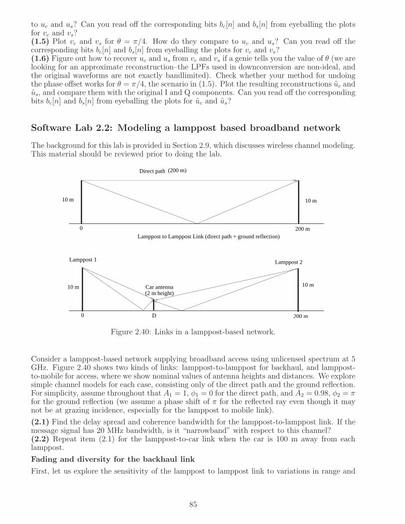
to uc and us? Can you read off the corresponding bits bc[n] and bs[n] from eyeballing the plotsfor vc and vs?(1.5) Plot vc and vs for θ = π/4. How do they compare to uc and us? Can you read off thecorresponding bits bc[n] and bs[n] from eyeballing the plots for vc and vs?(1.6) Figure out how to recover uc and us from vc and vs if a genie tells you the value of θ (we arelooking for an approximate reconstruction–the LPFs used in downconversion are non-ideal, andthe original waveforms are not exactly bandlimited). Check whether your method for undoingthe phase offset works for θ = π/4, the scenario in (1.5). Plot the resulting reconstructions uc andus, and compare them with the original I and Q components. Can you read off the correspondingbits bc[n] and bs[n] from eyeballing the plots for uc and us?

Software Lab 2.2: Modeling a lamppost based broadband network

The background for this lab is provided in Section 2.9, which discusses wireless channel modeling.This material should be reviewed prior to doing the lab.

Car antenna

Direct path

10 m10 m

(200 m)

Lamppost to Lamppost Link (direct path + ground reflection)

Lamppost 1 Lamppost 2

0 200 m

0 200 mD

10 m 10 m

(2 m height)

Figure 2.40: Links in a lamppost-based network.

Consider a lamppost-based network supplying broadband access using unlicensed spectrum at 5GHz. Figure 2.40 shows two kinds of links: lamppost-to-lamppost for backhaul, and lamppost-to-mobile for access, where we show nominal values of antenna heights and distances. We exploresimple channel models for each case, consisting only of the direct path and the ground reflection.For simplicity, assume throughout that A1 = 1, φ1 = 0 for the direct path, and A2 = 0.98, φ2 = πfor the ground reflection (we assume a phase shift of π for the reflected ray even though it maynot be at grazing incidence, especially for the lamppost to mobile link).

(2.1) Find the delay spread and coherence bandwidth for the lamppost-to-lamppost link. If themessage signal has 20 MHz bandwidth, is it “narrowband” with respect to this channel?(2.2) Repeat item (2.1) for the lamppost-to-car link when the car is 100 m away from eachlamppost.

Fading and diversity for the backhaul link

First, let us explore the sensitivity of the lamppost to lamppost link to variations in range and

85

height. Fix the height of the transmitter on lamppost 1 at 10 m. Vary the height of the receiveron lamppost 2 from 9.5 to 10.5 m.

(2.3) Letting hnom denote the nominal channel gain between two lampposts if you only considerthe direct path and h the net complex gain including the reflected path, plot the normalized

power gain in dB, 20 log10|h|

|hnom, as a function of the variation in the receiver height. Comment

on the sensitivity of channel quality to variations in the receiver height.(2.4) Modeling the variations in receiver height as coming from a uniform distribution over[9.5, 10.5], find the probability that the normalized power gain is smaller than -20 dB? (i.e., thatwe have a fade in signal power of 20 dB or worse).(2.5) Now, suppose that the transmitter has two antennas, vertically spaced by 25 cm, withthe lower one at a height of 10 m. Let h1 and h2 denote the channels from the two antennasto the receiver. Let hnom be defined as in item (2.3). Plot the normalized power gains in dB,

20 log10|hi|

|hnom| , i = 1, 2. Comment on whether or not both gains dip or peak at the same time.

(2.6) Plot 20 log10max(|h1|,|h2|)

|hnom| , which is the normalized power gain you would get if you switched

to the transmit antenna which has the better channel. This strategy is termed switched diversity.(2.7) Find the probability that the normalized power gain of the switched diversity scheme issmaller than -20 dB.(2.8) Comment on whether, and to what extent, diversity helped in combating fading.

Fading on the access link

Consider the access channel from lamppost 1 to the car. Let hnom(D) denote the nominal channelgain from the lamppost to the car, ignoring the ground reflection. Taking into account the groundreflection, let the channel gain be denoted as h(D). Here D is the distance of the car from thebottom of lamppost 1, as shown in Figure 2.40.

(2.9) Plot |hnom| and |h| as a function of D on a dB scale (an amplitude α is expressed on the dBscale as 20 log10 α). Comment on the “long-term” variation due to range, and the “short-term”variation due to multipath fading.

86

Chapter 3

Analog Communication Techniques

Modulation is the process of encoding information into a signal that can be transmitted (orrecorded) over a channel of interest. In analog modulation, a baseband message signal, suchas speech, audio or video, is directly transformed into a signal that can be transmitted overa designated channel, typically a passband radio frequency (RF) channel. Digital modulationdiffers from this only in the following additional step: bits are encoded into baseband messagesignals, which are then transformed into passband signals to be transmitted. Thus, despitethe relentless transition from digital to analog modulation, many of the techniques developed foranalog communication systems remain important for the digital communication systems designer,and our goal in this chapter is to study an important subset of these techniques, using legacyanalog communication systems as examples to reinforce concepts.

From Chapter 2, we know that passband signals carry information in their complex envelope,and that the complex envelope can be represented either in terms of I and Q components, or interms of envelope and phase. We study two broad classes of techniques: amplitude modula-tion, in which the analog message signal appears directly in the I and/or Q components; andangle modulation, in which the analog message signal appears directly in the phase or in theinstantaneous frequency (i.e., in the derivative of the phase), of the transmitted signal. Examplesof analog communication in space include AM radio, FM radio, and broadcast television, as wellas a variety of specialized radios. Examples of analog communication in time (i.e., for storage)include audiocassettes and VHS videotapes.

The analog-centric techniques covered in this chapter include envelope detection, superhetero-dyne reception, limiter discriminators, and phase locked loops. At a high level, these techniquestell us how to go from baseband message signals to passband transmitted signals, and backfrom passband received signals to baseband message signals. For analog communication, thisis enough, since we consider continuous time message signals which are directly transformed topassband through amplitude or angle modulation. For digital communication, we need to alsofigure out how to decode the encoded bits from the received passband signal, typically after down-conversion to baseband; this is a subject discussed in later chapters. However, between encodingat the transmitter and decoding at the receiver, a number of analog communication techniquesare relevant: for example, we need to decide between direct and superheterodyne architecturesfor upconversion and downconversion, and tailor our frequency planning appropriately; we mayuse a PLL to synthesize the local oscillator frequencies at the transmitter and receiver; andthe basic techniques for mapping baseband signals to passband remain the same (amplitudeand/or angle modulation). In addition, while many classical analog processing functionalitiesare replaced by digital signal processing in modern digital communication transceivers, when wepush the limits of digital communication systems, in terms of lowering power consumption orincreasing data rates, it is often necessary to fall back on analog-centric, or hybrid digital-analog,techniques. This is because the analog-to-digital conversion required for digital transceiver im-

87

plementations may often be too costly or power-hungry for ultra high-speed, or ultra low-power,implementations.

Chapter Plan: After a quick discussion of terminology and notation in Section 3.1, we discussvarious forms of amplitude modulation in Section 3.2, including bandwidth requirements and thetradeoffs between power efficiency and simplicity of demodulation. We discuss angle modulationin Section 3.3, including the relation between phase and frequency modulation, the bandwidthof angle modulated signals, and simple suboptimal demodulation strategies. The superhetero-dyne up/downconversion architecture is discussed in Section 3.4, and the design considerationsillustrated via the example of analog AM radio. The phase locked loop (PLL) is discussed inSection 3.5, including discussion of applications such as frequency synthesis and FM demodu-lation, linearized modeling and analysis, and a glimpse of the insights provided by nonlinearmodels. Finally, we discuss some legacy analog communication systems in Section 3.6, mainly tohighlight some of the creative design choices that were made in times when sophisticated digitalsignal processing techniques were not available. This last section can be skipped if the reader’sinterest is limited to learning analog-centric techniques for digital communication system design.

3.1 Terminology and notation

Message Signal: In the remainder of this chapter, the analog baseband message signal isdenoted by m(t). Depending on convenience of exposition, we shall think of this message aseither finite power or finite energy. In practice, any message we would encounter in practicewould have finite energy when we consider a finite time interval. However, when modelingtransmissions over long time intervals, it is useful to think of messages as finite power signalsspanning an infinite time interval. On the other hand, when discussing the effect of the messagespectrum on the spectrum of the transmitted signal, it may be convenient to consider a finiteenergy message signal. Since we consider physical message signals, the time domain signal is real-valued, so that its Fourier transform (defined for a finite energy signal) is conjugate symmetric:M(f) = M∗(−f). For a finite power (infinite energy) message, recall from Chapter 2 that thepower is defined as a time average in the limit of an infinite observation interval, as follows:

m2 = limTo→∞

1

To

∫ To

0

m2(t)dt

Similarly, the DC value is defined as

m = limTo→∞

1

To

∫ To

0

m(t)dt

We typically assume that the DC value of the message is zero: m = 0.

A simple example, shown in Figure 3.1, that we shall use often is a finite-power sinusoidalmessage signal, m(t) = Am cos 2πfmt, whose spectrum consists of impulses at ±fm: M(f) =Am

2(δ(f − fm) + δ(f + fm)). For this message, m = 0 and m2 = A2

m/2.

Transmitted Signal: When the signal transmitted over the channel is a passband signal, itcan be written as (see Chapter 2)

up(t) = uc(t) cos(2πfct)− us(t) sin(2πfct) = e(t) cos(2πfct+ θ(t))

where fc is a carrier frequency, uc(t) is the I component, us(t) is the Q component, e(t) ≥ 0 is theenvelope, and θ(t) is the phase. Modulation consist of encoding the message in uc(t) and us(t), orequivalently, in e(t) and θ(t). In most of the analog amplitude modulation schemes considered,

88

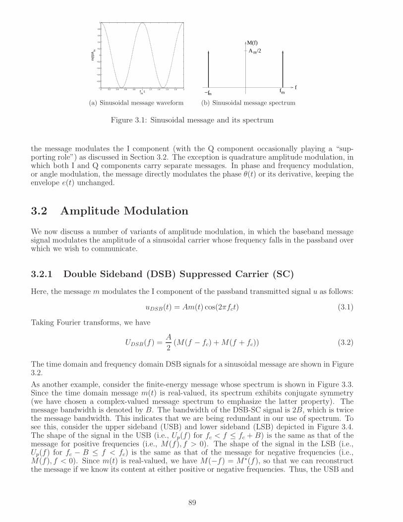
0 0.2 0.4 0.6 0.8 1 1.2 1.4 1.6 1.8 2−1

−0.8

−0.6

−0.4

−0.2

0

0.2

0.4

0.6

0.8

1

fm

tm

(t)/

Am

(a) Sinusoidal message waveform

f

m

m−f fm

M(f)

A /2

(b) Sinusoidal message spectrum

Figure 3.1: Sinusoidal message and its spectrum

the message modulates the I component (with the Q component occasionally playing a “sup-porting role”) as discussed in Section 3.2. The exception is quadrature amplitude modulation, inwhich both I and Q components carry separate messages. In phase and frequency modulation,or angle modulation, the message directly modulates the phase θ(t) or its derivative, keeping theenvelope e(t) unchanged.

3.2 Amplitude Modulation

We now discuss a number of variants of amplitude modulation, in which the baseband messagesignal modulates the amplitude of a sinusoidal carrier whose frequency falls in the passband overwhich we wish to communicate.

3.2.1 Double Sideband (DSB) Suppressed Carrier (SC)

Here, the message m modulates the I component of the passband transmitted signal u as follows:

uDSB(t) = Am(t) cos(2πfct) (3.1)

Taking Fourier transforms, we have

UDSB(f) =A

2(M(f − fc) +M(f + fc)) (3.2)

The time domain and frequency domain DSB signals for a sinusoidal message are shown in Figure3.2.

As another example, consider the finite-energy message whose spectrum is shown in Figure 3.3.Since the time domain message m(t) is real-valued, its spectrum exhibits conjugate symmetry(we have chosen a complex-valued message spectrum to emphasize the latter property). Themessage bandwidth is denoted by B. The bandwidth of the DSB-SC signal is 2B, which is twicethe message bandwidth. This indicates that we are being redundant in our use of spectrum. Tosee this, consider the upper sideband (USB) and lower sideband (LSB) depicted in Figure 3.4.The shape of the signal in the USB (i.e., Up(f) for fc < f ≤ fc + B) is the same as that of themessage for positive frequencies (i.e., M(f), f > 0). The shape of the signal in the LSB (i.e.,Up(f) for fc − B ≤ f < fc) is the same as that of the message for negative frequencies (i.e.,M(f), f < 0). Since m(t) is real-valued, we have M(−f) = M∗(f), so that we can reconstructthe message if we know its content at either positive or negative frequencies. Thus, the USB and

89

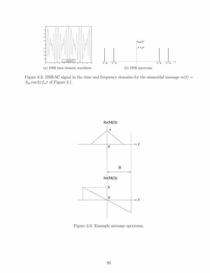
0 2 4 6 8 10 12 14 16 18 20−1

−0.8

−0.6

−0.4

−0.2

0

0.2

0.4

0.6

0.8

1

message waveformDSB waveform

(a) DSB time domain waveform

f−f + fm cf − fm cf + fm

A A /4m

U (f)DSB

c−f −fm c

(b) DSB spectrum

Figure 3.2: DSB-SC signal in the time and frequency domains for the sinusoidal message m(t) =Am cos 2πfmt of Figure 3.1.

b

B

Re(M(f))

Im(M(f))

f

f0

0

a

Figure 3.3: Example message spectrum.

90

A b/2

DSB

−fc fc

−fc fc

Im(U (f))DSB

LowerSideband

UpperSideband

UpperSideband

LowerSideband

2B

f

f

A a/2

Re(U (f))

Figure 3.4: The spectrum of the passband DSB-SC signal for the example message in Figure 3.3.

LSB of u(t) each contain enough information to reconstruct the message. The term DSB refers tothe fact that we are sending both sidebands. Doing this, of course, is wasteful of spectrum. Thismotivates single sideband (SSB) and vestigial sideband (VSB) modulation, which are discusseda little later.

The term suppressed carrier is employed because, for a message with no DC component, wesee from (3.2) that the transmitted signal does not have a discrete component at the carrierfrequency (i.e., Up(f) does not have impulses at ±fc).

messageLowpass

Filter

π2cos 2 f tc

Passband receivedsignal

Estimated

Figure 3.5: Coherent demodulation for AM.

Demodulation of DSB-SC: Since the message is contained in the I component, demodulationconsists of extracting the I component of the received signal, which we know how to do fromChapter 2: multiply the received signal with the cosine of the carrier, and pass it through a lowpass filter. Ignoring noise, the received signal is given by

yp(t) = Am(t) cos(2πfct+ θr) (3.3)

where θr is the phase of the received carrier relative to the local copy of the carrier producedby the receiver’s local oscillator (LO), and A is the received amplitude, taking into account thepropagation channel from the transmitter to the receiver. The demodulator is shown in Figure3.5. In order for this demodulator to work well, we must have θr as close to zero as possible;that is, the carrier produced by the LO must be coherent with the received carrier. To see theeffect of phase mismatch, let us compute the demodulator output for arbitrary θr. Using thetrigonometric identity 2 cos θ1 cos θ2 = cos(θ1 − θ2) + cos(θ1 + θ2), we have

2yp(t) cos(2πfct) = Am(t) cos(2πfct + θr) cos(2πfct) = Am(t) cos θr + Am(t) cos(4πfct + θr)

91

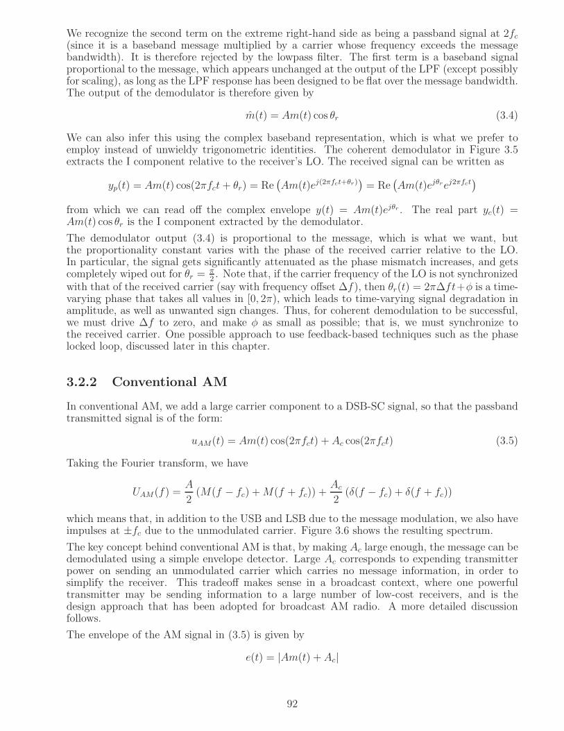
We recognize the second term on the extreme right-hand side as being a passband signal at 2fc(since it is a baseband message multiplied by a carrier whose frequency exceeds the messagebandwidth). It is therefore rejected by the lowpass filter. The first term is a baseband signalproportional to the message, which appears unchanged at the output of the LPF (except possiblyfor scaling), as long as the LPF response has been designed to be flat over the message bandwidth.The output of the demodulator is therefore given by

m(t) = Am(t) cos θr (3.4)

We can also infer this using the complex baseband representation, which is what we prefer toemploy instead of unwieldy trigonometric identities. The coherent demodulator in Figure 3.5extracts the I component relative to the receiver’s LO. The received signal can be written as

yp(t) = Am(t) cos(2πfct+ θr) = Re(

Am(t)ej(2πfct+θr))

= Re(

Am(t)ejθrej2πfct)

from which we can read off the complex envelope y(t) = Am(t)ejθr . The real part yc(t) =Am(t) cos θr is the I component extracted by the demodulator.

The demodulator output (3.4) is proportional to the message, which is what we want, butthe proportionality constant varies with the phase of the received carrier relative to the LO.In particular, the signal gets significantly attenuated as the phase mismatch increases, and getscompletely wiped out for θr =

π2. Note that, if the carrier frequency of the LO is not synchronized

with that of the received carrier (say with frequency offset ∆f), then θr(t) = 2π∆ft+φ is a time-varying phase that takes all values in [0, 2π), which leads to time-varying signal degradation inamplitude, as well as unwanted sign changes. Thus, for coherent demodulation to be successful,we must drive ∆f to zero, and make φ as small as possible; that is, we must synchronize tothe received carrier. One possible approach to use feedback-based techniques such as the phaselocked loop, discussed later in this chapter.

3.2.2 Conventional AM

In conventional AM, we add a large carrier component to a DSB-SC signal, so that the passbandtransmitted signal is of the form:

uAM(t) = Am(t) cos(2πfct) + Ac cos(2πfct) (3.5)

Taking the Fourier transform, we have

UAM(f) =A

2(M(f − fc) +M(f + fc)) +

Ac

2(δ(f − fc) + δ(f + fc))

which means that, in addition to the USB and LSB due to the message modulation, we also haveimpulses at ±fc due to the unmodulated carrier. Figure 3.6 shows the resulting spectrum.

The key concept behind conventional AM is that, by making Ac large enough, the message can bedemodulated using a simple envelope detector. Large Ac corresponds to expending transmitterpower on sending an unmodulated carrier which carries no message information, in order tosimplify the receiver. This tradeoff makes sense in a broadcast context, where one powerfultransmitter may be sending information to a large number of low-cost receivers, and is thedesign approach that has been adopted for broadcast AM radio. A more detailed discussionfollows.

The envelope of the AM signal in (3.5) is given by

e(t) = |Am(t) + Ac|

92

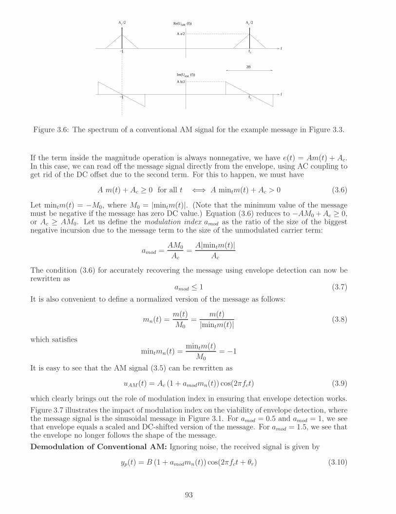
AM

−fc fc

−fc fc

cA /2 cA /2

f

f

A a/2

A b/2

2B

Re(U (f))AM

Im(U (f))

Figure 3.6: The spectrum of a conventional AM signal for the example message in Figure 3.3.

If the term inside the magnitude operation is always nonnegative, we have e(t) = Am(t) + Ac.In this case, we can read off the message signal directly from the envelope, using AC coupling toget rid of the DC offset due to the second term. For this to happen, we must have

A m(t) + Ac ≥ 0 for all t ⇐⇒ A mintm(t) + Ac > 0 (3.6)

Let mintm(t) = −M0, where M0 = |mintm(t)|. (Note that the minimum value of the messagemust be negative if the message has zero DC value.) Equation (3.6) reduces to −AM0 +Ac ≥ 0,or Ac ≥ AM0. Let us define the modulation index amod as the ratio of the size of the biggestnegative incursion due to the message term to the size of the unmodulated carrier term:

amod =AM0

Ac

=A|mintm(t)|

Ac

The condition (3.6) for accurately recovering the message using envelope detection can now berewritten as

amod ≤ 1 (3.7)

It is also convenient to define a normalized version of the message as follows:

mn(t) =m(t)

M0

=m(t)

|mintm(t)| (3.8)

which satisfies

mintmn(t) =mintm(t)

M0

= −1

It is easy to see that the AM signal (3.5) can be rewritten as

uAM(t) = Ac (1 + amodmn(t)) cos(2πfct) (3.9)

which clearly brings out the role of modulation index in ensuring that envelope detection works.

Figure 3.7 illustrates the impact of modulation index on the viability of envelope detection, wherethe message signal is the sinusoidal message in Figure 3.1. For amod = 0.5 and amod = 1, we seethat envelope equals a scaled and DC-shifted version of the message. For amod = 1.5, we see thatthe envelope no longer follows the shape of the message.

Demodulation of Conventional AM: Ignoring noise, the received signal is given by

yp(t) = B (1 + amodmn(t)) cos(2πfct + θr) (3.10)

93

0 2 4 6 8 10 12 14 16 18 20−1.5

−1

−0.5

0

0.5

1

1.5

envelopeAM waveform

(a) Modulation Index amod = 0.5

0 2 4 6 8 10 12 14 16 18 20−2

−1.5

−1

−0.5

0

0.5

1

1.5

2

envelopeAM waveform

(b) Modulation Index amod = 1.0

0 2 4 6 8 10 12 14 16 18 20−2.5

−2

−1.5

−1

−0.5

0

0.5

1

1.5

2

2.5

envelopeAM waveform

(c) Modulation Index amod = 1.5

Figure 3.7: Time domain AM waveforms for a sinusoidal message. The envelope no longer followsthe message for modulation index larger than one.

94

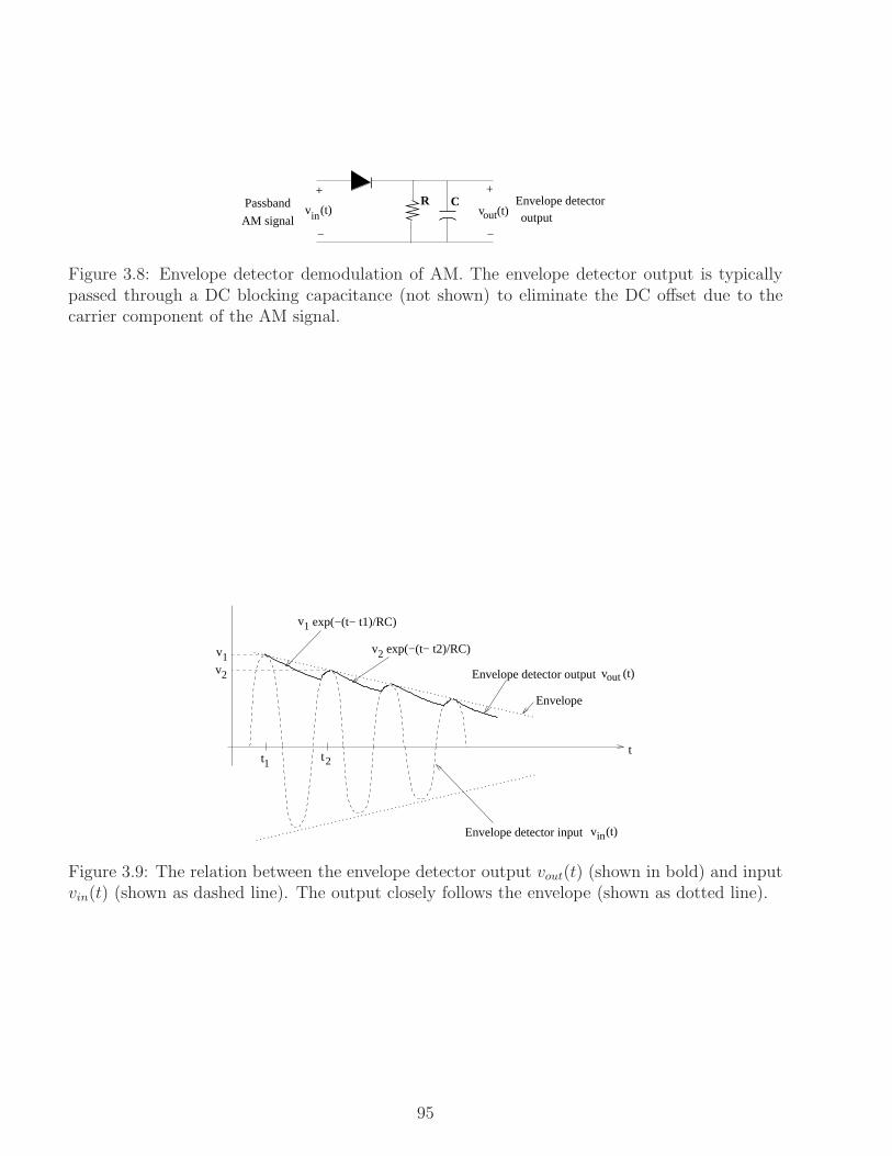
outputv (t)in v (t)out

+

−

R C+

−

Passband

AM signal

Envelope detector

Figure 3.8: Envelope detector demodulation of AM. The envelope detector output is typicallypassed through a DC blocking capacitance (not shown) to eliminate the DC offset due to thecarrier component of the AM signal.

exp(−(t− t2)/RC)1

t1 t2

v2 v (t)out

inv (t)

v2

v1

t

Envelope detector output

Envelope detector input

Envelope

exp(−(t− t1)/RC)

v

Figure 3.9: The relation between the envelope detector output vout(t) (shown in bold) and inputvin(t) (shown as dashed line). The output closely follows the envelope (shown as dotted line).

95

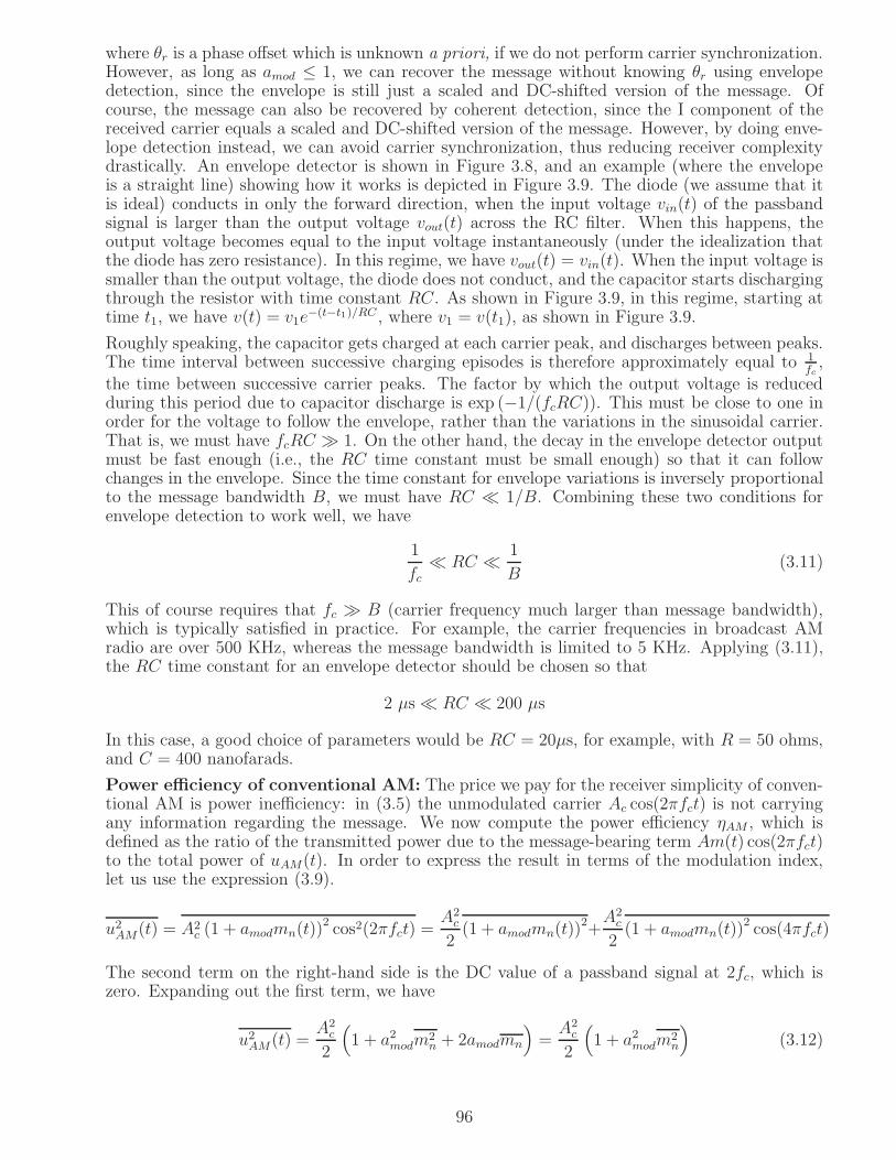
where θr is a phase offset which is unknown a priori, if we do not perform carrier synchronization.However, as long as amod ≤ 1, we can recover the message without knowing θr using envelopedetection, since the envelope is still just a scaled and DC-shifted version of the message. Ofcourse, the message can also be recovered by coherent detection, since the I component of thereceived carrier equals a scaled and DC-shifted version of the message. However, by doing enve-lope detection instead, we can avoid carrier synchronization, thus reducing receiver complexitydrastically. An envelope detector is shown in Figure 3.8, and an example (where the envelopeis a straight line) showing how it works is depicted in Figure 3.9. The diode (we assume that itis ideal) conducts in only the forward direction, when the input voltage vin(t) of the passbandsignal is larger than the output voltage vout(t) across the RC filter. When this happens, theoutput voltage becomes equal to the input voltage instantaneously (under the idealization thatthe diode has zero resistance). In this regime, we have vout(t) = vin(t). When the input voltage issmaller than the output voltage, the diode does not conduct, and the capacitor starts dischargingthrough the resistor with time constant RC. As shown in Figure 3.9, in this regime, starting attime t1, we have v(t) = v1e

−(t−t1)/RC , where v1 = v(t1), as shown in Figure 3.9.

Roughly speaking, the capacitor gets charged at each carrier peak, and discharges between peaks.The time interval between successive charging episodes is therefore approximately equal to 1

fc,

the time between successive carrier peaks. The factor by which the output voltage is reducedduring this period due to capacitor discharge is exp (−1/(fcRC)). This must be close to one inorder for the voltage to follow the envelope, rather than the variations in the sinusoidal carrier.That is, we must have fcRC ≫ 1. On the other hand, the decay in the envelope detector outputmust be fast enough (i.e., the RC time constant must be small enough) so that it can followchanges in the envelope. Since the time constant for envelope variations is inversely proportionalto the message bandwidth B, we must have RC ≪ 1/B. Combining these two conditions forenvelope detection to work well, we have

1

fc≪ RC ≪ 1

B(3.11)

This of course requires that fc ≫ B (carrier frequency much larger than message bandwidth),which is typically satisfied in practice. For example, the carrier frequencies in broadcast AMradio are over 500 KHz, whereas the message bandwidth is limited to 5 KHz. Applying (3.11),the RC time constant for an envelope detector should be chosen so that

2 µs ≪ RC ≪ 200 µs

In this case, a good choice of parameters would be RC = 20µs, for example, with R = 50 ohms,and C = 400 nanofarads.

Power efficiency of conventional AM: The price we pay for the receiver simplicity of conven-tional AM is power inefficiency: in (3.5) the unmodulated carrier Ac cos(2πfct) is not carryingany information regarding the message. We now compute the power efficiency ηAM , which isdefined as the ratio of the transmitted power due to the message-bearing term Am(t) cos(2πfct)to the total power of uAM(t). In order to express the result in terms of the modulation index,let us use the expression (3.9).

u2AM(t) = A2c (1 + amodmn(t))

2 cos2(2πfct) =A2

c

2(1 + amodmn(t))

2+A2

c

2(1 + amodmn(t))

2 cos(4πfct)

The second term on the right-hand side is the DC value of a passband signal at 2fc, which iszero. Expanding out the first term, we have

u2AM(t) =A2

c

2

(

1 + a2modm2n + 2amodmn

)

=A2

c

2

(

1 + a2modm2n

)

(3.12)

96

assuming that the message has zero DC value. The power of the message-bearing term can besimilarly computed as

(Acamodmn(t))2 cos2(2πfct) =

A2c

2a2modm

2n

so that the power efficiency is given by

ηAM =a2modm

2n

1 + a2modm2n

(3.13)

Noting that mn is normalized so that its most negative value is −1, for messages which havecomparable positive and negative excursions around zero, we expect |mn(t)| ≤ 1, and hence

average power m2n ≤ 1 (typical values are much smaller than one). Since amod ≤ 1 for envelope

detection to work, the power efficiency of conventional AM is at best 50%. For a sinusoidalmessage, for example, it is easy to see thatm2

n = 1/2, so that the power efficiency is at most 33%.For speech signals, which have significantly higher peak-to-average ratio, the power efficiency iseven smaller.

Example 3.2.1 (AM power efficiency computation): The message m(t) = 2 sin 2000πt−3 cos 4000πt is used in an AM system with a modulation index of 70% and carrier frequencyof 580 KHz. What is the power efficiency? If the net transmitted power is 10 watts, find themagnitude spectrum of the transmitted signal.We need to find M0 = |mintm(t)| in order to determine the normalized form mn(t) = m(t)/M0.To simplify notation, let x = 2000πt, and minimize g(x) = 2 sin x− 3 cos 2x. Since g is periodicwith period 2π, we can minimize it numerically over a period. However, we can perform theminimization analytically in this case. Differentiating g, we obtain

g′(x) = 2 cosx+ 6 sin 2x = 0

This gives2 cosx+ 12 sinx cos x = 2 cosx(1 + 6 sin x) = 0

There are two solutions cosx = 0 and sin x = −16. The first solution gives cos 2x = 2 cos2 x−1 =

−1 and sin x = ±1, which gives g(x) = 1, 5. The second solution gives cos 2x = 1 − 2 sin2 x =1− 2/36 = 17/18, which gives g(x) = 2(−1/6)− 3(17/18) = −19/6. We therefore obtain

M0 = |mintm(t)| = 19/6

This gives

mn(t) =m(t)

M0=

12

19sin 10πt− 18

19cos 20πt

This givesm2

n = (12/19)2(1/2) + (18/19)2(1/2) = 0.65

Substituting in (3.13), setting amod = 0.7, we obtain a power efficiency ηAM = 0.24, or 24%.To figure out the spectrum of the transmitted signal, we must find Ac in the formula (3.9). Thepower of the transmitted signal is given by (3.12) to be

10 =A2

c

2

(

1 + a2modm2n

)

=A2

c

2

(

1 + (0.72)(0.65))

which yields Ac ≈ 3.9. The overall AM signal is given by

uAM(t) = Ac(1 + amodmn(t)) cos 2πfct = Ac (1 + a1 sin 2πf1t+ a2 cos 4πf1t) cos 2πfct

97

where a1 = 0.7(12/19) = 0.44, a2 = 0.7(−18/19) = −0.66, f1 = 1 KHz and fc = 580KHz. Themagnitude spectrum is given by

|UAM(f)| = Ac/2 (δ(f − fc) + δ(f + fc))+ Ac|a1|/4 (δ(f − fc − f1) + δ(f − fc + f1) + δ(f + fc + f1) + δ(f + fc − f1))

+ Ac|a2|/4 (δ(f − fc − 2f1) + δ(f − fc + 2f1) + δ(f + fc + 2f1) + δ(f + fc − 2f1))

with numerical values shown in Figure 3.10.

0.644

AM

~ ~ ~ ~

f (KHz)−578 −579−580 −581 −582 579578 580 581 582

1.951.95

0.429 0.429 0.429 0.429

0.6440.6440.644

|U (f)|

Figure 3.10: Magnitude spectrum for the AM waveform in Example 3.2.1.

3.2.3 Single Sideband Modulation (SSB)

In SSB modulation, we send either the upper sideband or the lower sideband of a DSB-SC signal.For the running example, the spectra of the passband USB and LSB signals are shown in Figure3.11.

From our discussion of DSB-SC, we know that each sideband provides enough information toreconstruct the message. But how do we physically reconstruct the message from an SSB signal?To see this, consider the USB signal depicted in Figure 3.11(a). We can reconstruct the basebandmessage if we can move the component near +fc to the left by fc, and the component near −fcto the right by fc; that is, if we move in the passband components towards the origin. Thesetwo frequency translations can be accomplished by multiplying the USB signal by 2 cos 2πfct =ej2πfct + e−j2πfct, as shown in Figure 3.5, which creates the desired message signal at baseband,as well as undesired frequency components at ±2fc which can be rejected by a lowpass filter. Itcan be checked that the same argument applies to LSB signals as well.

It follows from the preceding discussion that SSB signals can be demodulated in exactly thesame fashion as DSB-SC, using the coherent demodulator depicted in Figure 3.5. Since thisdemodulator simply extracts the I component of the passband signal, the I component of theSSB signal must be the message. In order to understand the structure of an SSB signal, it remainsto identify the Q component. This is most easily done by considering the complex envelope ofthe passband transmitted signal. Consider again the example USB signal in Figure 3.11(a). Thespectrum U(f) of its complex envelope relative to fc is shown in Figure 3.12. Now, the spectraof I and Q components can be inferred as follows:

Uc(f) =U(f) + U∗(−f)

2, Us(f) =

U(f)− U∗(−f)2j

Applying these equations, we get I and Q components as shown in Figure 3.13.

98

B

c fc

−fc fc

f

f

A a/2

A b/2

Im(U (f))

Re(U (f))USB

USB

−f

(a) Upper Sideband Signaling

B

c fc

−fc fc

f

f

A a/2

A b/2

Re(U (f))

Im(U (f))LSB

LSB

−f

(b) Lower Sideband Signaling

Figure 3.11: Spectra for SSB signaling for the example message in Figure 3.3.

Im(U(f))

f

Aa

Re(U(f))

f

−Ab

f

Figure 3.12: Complex envelope for the USB signal in Figure 3.11(a).

99

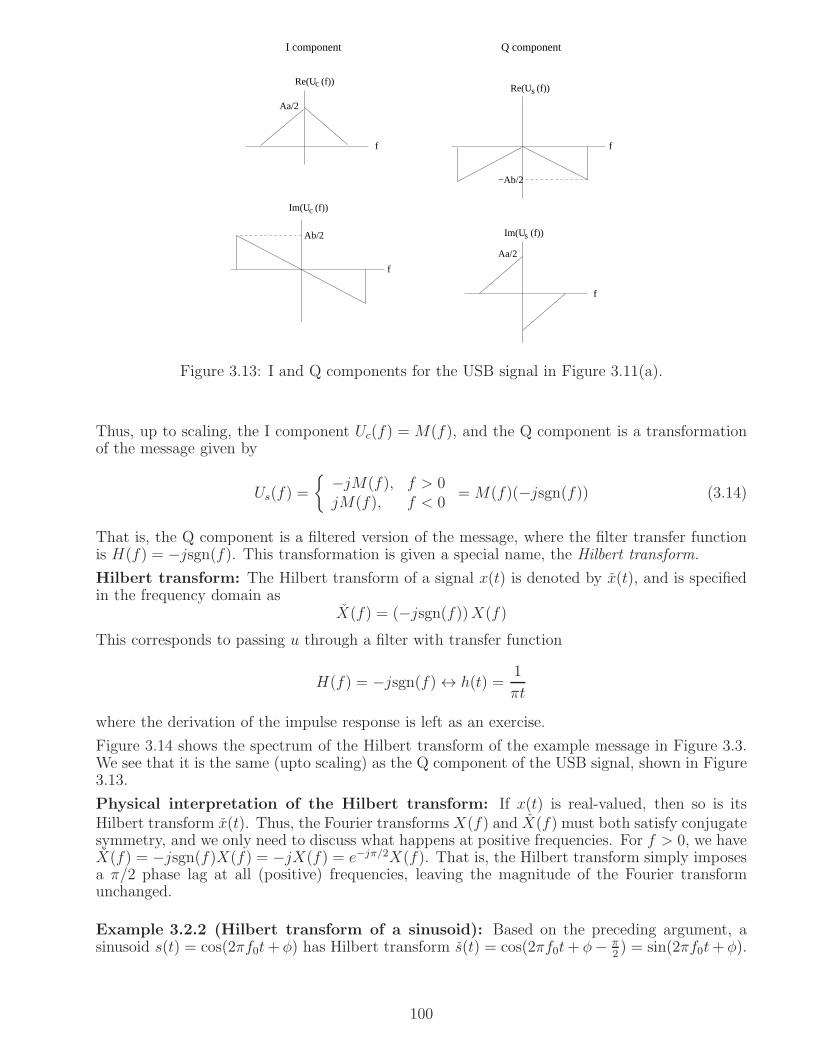
I component

Ab/2

f

Im(U (f))c

Aa/2

f

Re(U (f))c

f

−Ab/2

Aa/2

f

sIm(U (f))

Re(U (f))s

Q component

Figure 3.13: I and Q components for the USB signal in Figure 3.11(a).

Thus, up to scaling, the I component Uc(f) = M(f), and the Q component is a transformationof the message given by

Us(f) =

−jM(f), f > 0jM(f), f < 0

=M(f)(−jsgn(f)) (3.14)

That is, the Q component is a filtered version of the message, where the filter transfer functionis H(f) = −jsgn(f). This transformation is given a special name, the Hilbert transform.

Hilbert transform: The Hilbert transform of a signal x(t) is denoted by x(t), and is specifiedin the frequency domain as

X(f) = (−jsgn(f))X(f)

This corresponds to passing u through a filter with transfer function

H(f) = −jsgn(f) ↔ h(t) =1

πt

where the derivation of the impulse response is left as an exercise.

Figure 3.14 shows the spectrum of the Hilbert transform of the example message in Figure 3.3.We see that it is the same (upto scaling) as the Q component of the USB signal, shown in Figure3.13.

Physical interpretation of the Hilbert transform: If x(t) is real-valued, then so is itsHilbert transform x(t). Thus, the Fourier transforms X(f) and X(f) must both satisfy conjugatesymmetry, and we only need to discuss what happens at positive frequencies. For f > 0, we haveX(f) = −jsgn(f)X(f) = −jX(f) = e−jπ/2X(f). That is, the Hilbert transform simply imposesa π/2 phase lag at all (positive) frequencies, leaving the magnitude of the Fourier transformunchanged.

Example 3.2.2 (Hilbert transform of a sinusoid): Based on the preceding argument, asinusoid s(t) = cos(2πf0t+ φ) has Hilbert transform s(t) = cos(2πf0t+ φ− π

2) = sin(2πf0t+ φ).

100

−b

Im(M(f))

Re(M(f))

B

f

f0

0

a

Figure 3.14: Spectrum of the Hilbert transform of the example message in Figure 3.3.

We can also do this the hard way, as follows:

s(t) = cos(2πf0t+ φ) = 12

(

ej(2πf0t+φ) + e−j(2πf0t+φ))

↔ S(f) = 12

(

ejφδ(f − f0) + e−jφδ(f + f0))

Thus,S(f) = −jsgn(f)S(f) = 1

2

(

ejφ(−j)δ(f − f0) + e−jφ(j)δ(f + f0))

↔ s(t) = 12

(

ejφ(−j)ej2πf0t + e−jφ(j)ej2πf0t)

which simplifies to

s(t) =1

2j

(

ej(2πf0t+φ) − e−j(2πf0t+φ))

= sin(2πf0t+ φ)

Equation (3.14) shows that the Q component of the USB signal is m(t), the Hilbert transformof the message. Thus, the passband USB signal can be written as

uUSB(t) = m(t) cos(2πfct)− m(t) sin(2πfct) (3.15)

Similarly, we can show that the Q component of an LSB signal is −m(t), so that the passbandLSB signal is given by

uLSB(t) = m(t) cos(2πfct) + m(t) sin(2πfct) (3.16)

SSB modulation: Conceptually, an SSB signal can be generated by filtering out one of thesidebands of a DSB-SC signal. However, it is difficult to implement the required sharp cutoffat fc, especially if we wish to preserve the information contained at the boundary of the twosidebands, which corresponds to the message information near DC. Thus, an implementation ofSSB based on sharp bandpass filters runs into trouble when the message has significant frequencycontent near DC. The representations in (3.15) and (3.16) provide an alternative approach togenerating SSB signals, as shown in Figure 3.15. We have emphasized the role of 90 phase lagsin generating the I and Q components, as well as the LO signals used for upconversion.

Example 3.2.3 (SSB waveforms for a sinusoidal message): For a sinusoidal messagem(t) = cos 2πfmt, we have m(t) = sin 2πfmt from Example 3.2.2. Consider the DSB signal

uDSB(t) = 2 cos 2πfmt cos 2πfct

101

over message band)

2cos 2 f tc

m(t)

2sin 2 f tπ c

Local

Oscillator

90 deg

m(t)

Hilbert transform(90 deg phase lag

phase lag −/+

Message signal

USB/LSB signal

π

Figure 3.15: SSB modulation using the Hilbert transform of the message.

USB

DSB

~ ~~ ~

c−f + fmc−f −fm cf − fm cf + fm

1/2

f

~ ~~ ~

~ ~~ ~

c−f −fm cf + fm

c−f + fm cf − fm

1/2

f

U (f)

1/2

f

U (f)LSB

U (f)

Figure 3.16: DSB and SSB spectra for a sinusoidal message.

102

where we have normalized the signal power to one: u2DSB = 1. The DSB, USB and SSB spectrumare shown in Figure 3.16. From the SSB spectra shown, we can immediately write down thefollowing time domain expressions:

uUSB(t) = cos 2π(fc + fm)t = cos 2πfmt cos 2πfct− sin 2πfmt sin 2πfct

uLSB(t) = cos 2π(fc − fm)t = cos 2πfmt cos 2πfct + sin 2πfmt sin 2πfct

The preceding equations are consistent with (3.15) and (3.16). For both the USB and LSBsignals, the I component equals the message: uc(t) = m(t) = cos 2πfmt. The Q componentfor the USB signal is us(t) = m(t) = sin 2πfmt, and the Q component for the LSB signal isus(t) = −m(t) = − sin 2πfmt.

SSB demodulation: We know now that the message can be recovered from an SSB signalby extracting its I component using a coherent demodulator as in Figure 3.5. The difficulty ofcoherent demodulation lies in the requirement for carrier synchronization, and we have discussedthe adverse impact of imperfect synchronization for DSB-SC signals. We now show that theperformance degradation is even more significant for SSB signals. Consider a USB receivedsignal of the form (ignoring scale factors):

yp(t) = m(t) cos(2πfct+ θr)− m(t) sin(2πfct + θr) (3.17)

where θr is the phase offset with respect to the receiver LO. The complex envelope with respectto the receiver LO is given by

y(t) = (m(t) + jm(t)) ejθr = (m(t) + jm(t)) (cos θr + j sin θr)

Taking the real part, we obtain that the I component extracted by the coherent demodulator is

yc(t) = m(t) cos θr − m(t) sin θr

Thus, as the phase error θr increases, not only do we get an attenuation in the first term corre-sponding to the desired message (as in DSB), but we also get interference due to the second termfrom the Hilbert transform of the message. Thus, for coherent demodulation, accurate carriersynchronization is even more crucial for SSB than for DSB.

Noncoherent demodulation is also possible for SSB if we add a strong carrier term, as in conven-tional AM. Specifically, for a received signal given by

yp(t) = (A+m(t)) cos(2πfct + θr)± m(t) sin(2πfct+ θr)

the envelope is given by

e(t) =√

(A+m(t))2 + m2(t) ≈ A+m(t) (3.18)

if |A+m(t)| ≫ |m(t)|. Subject to the approximation in (3.18), an envelope detector works justas in conventional AM.

3.2.4 Vestigial Sideband (VSB) Modulation

VSB is similar to SSB, in that it also tries to reduce the transmitted bandwidth relative to DSB,and the transmitted signal is a filtered version of the DSB signal. The idea is to mainly transmitone of the two sidebands, but to leave a vestige of the other sideband in order to ease the filteringrequirements. The passband filter used to shape the DSB signal in this fashion is chosen so that

103

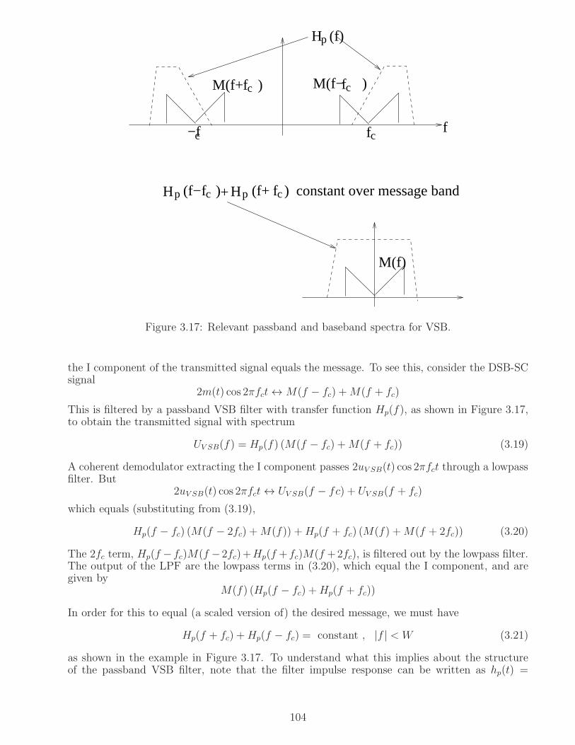
constant over message band

fc−fc

Hp fc(f+ )Hp fc(f− )+

fcM(f+ ) fcM(f− )

M(f)

f

H (f)p

Figure 3.17: Relevant passband and baseband spectra for VSB.

the I component of the transmitted signal equals the message. To see this, consider the DSB-SCsignal

2m(t) cos 2πfct↔ M(f − fc) +M(f + fc)

This is filtered by a passband VSB filter with transfer function Hp(f), as shown in Figure 3.17,to obtain the transmitted signal with spectrum

UV SB(f) = Hp(f) (M(f − fc) +M(f + fc)) (3.19)

A coherent demodulator extracting the I component passes 2uV SB(t) cos 2πfct through a lowpassfilter. But

2uV SB(t) cos 2πfct↔ UV SB(f − fc) + UV SB(f + fc)

which equals (substituting from (3.19),

Hp(f − fc) (M(f − 2fc) +M(f)) +Hp(f + fc) (M(f) +M(f + 2fc)) (3.20)

The 2fc term, Hp(f −fc)M(f −2fc)+Hp(f +fc)M(f +2fc), is filtered out by the lowpass filter.The output of the LPF are the lowpass terms in (3.20), which equal the I component, and aregiven by

M(f) (Hp(f − fc) +Hp(f + fc))

In order for this to equal (a scaled version of) the desired message, we must have

Hp(f + fc) +Hp(f − fc) = constant , |f | < W (3.21)

as shown in the example in Figure 3.17. To understand what this implies about the structureof the passband VSB filter, note that the filter impulse response can be written as hp(t) =

104

hc(t) cos 2πfct − hs(t) sin 2πfct, where hc(t) is obtained by passing 2hp(t) cos(2πfct) through alowpass filter. But 2hp(t) cos(2πfct) ↔ Hp(f − fc) + Hp(f + fc). Thus, the Fourier transforminvolved in (3.21) is precisely the lowpass restriction of 2hp(t) cos(2πfct), i.e., it is Hc(f). Thus,the correct demodulation condition for VSB in (3.21) is equivalent to requiring that Hc(f) beconstant over the message band. Further discussion of the structure of VSB signals is providedvia problems.

As with SSB, if we add a strong carrier component to the VSB signal, we can demodulate itnoncoherently using an envelope detector, again at the cost of some distortion from the presenceof the Q component.

3.2.5 Quadrature Amplitude Modulation

The transmitted signal in quadrature amplitude modulation (QAM) is of the form

uQAM(t) = mc(t) cos 2πfct−ms(t) sin 2πfct

where mc(t) and ms(t) are separate messages (unlike SSB and VSB, where the Q component isa transformation of the message carried by the I component). In other words, a complex-valuedmessage m = mc(t) + jms(t) is encoded in the complex envelope of the passband transmittedsignal. QAM is extensively employed in digital communication, as we shall see in later chapters.It is also used to carry color information in analog TV.

signal

LowpassFilter

LowpassFilter

cm (t)^

m (t)s^

f c−2 sin 2 tπ

f c2 cos 2 tπPassbandQAM

Figure 3.18: Demodulation for quadrature amplitude modulation.

Demodulation is achieved using a coherent receiver which extracts both the I and Q components,as shown in Figure 3.18. If the received signal has a phase offset θ relative to the receiver’s LO,then we get both attenuation in the desired message and interference from the undesired message,as follows. Ignoring noise and scale factors, the reconstructed complex baseband message is givenby

m(t) = mc(t) + jms(t) = (mc(t) + jms(t))ejθ(t) = m(t)ejθ(t)

from which we conclude that

mc(t) = mc(t) cos θ(t)−ms(t) sin θ(t)ms(t) = ms(t) cos θ(t) +mc(t) sin θ(t)

Thus, accurate carrier synchronization (θ(t) as close to zero as possible) is important for QAMdemodulation to function properly.

105

−1/2

f (KHz)

M(f)

10−10

20−20

1

−1/2

1

(a) Message spectrum

not shown)

600 610

620

590

580f (KHz)

X(f)

5/2

1/21/2

−1/4 −1/4

(spectrum fornegative frequencies

(b) AM spectrum

Figure 3.19: Spectrum of message and the corresponding AM signal in Example 3.2.4. Axes arenot to scale.

Y(f)

f (KHz)

5/2

1/2

−1/4

(spectrum fornegative frequenciesnot shown)

600 610

620

(a) Passband output of BPF

5

Y(f)

f (KHz)10

1

−1/2

20

0

~

(b) Complex envelope

Figure 3.20: Passband output of bandpass filter and its complex envelope with respect to 600KHz reference, for Example 3.2.4. Axes are not to scale.

3.2.6 Concept synthesis for AM

Here is a worked problem that synthesizes a few of the concepts we have discussed for AM.

Example 3.2.4 The signal m(t) = 2 cos 20πt− cos 40πt, where the unit of time is millisec-onds, is amplitude modulated using a carrier frequency fc of 600 KHz. The AM signal is givenby

x(t) = 5 cos 2πfct+m(t) cos 2πfct

(a) Sketch the magnitude spectrum of x. What is its bandwidth?(b) What is the modulation index?(c) The AM signal is passed through an ideal highpass filter with cutoff frequency 595 KHz (i.e.,the filter passes all frequencies above 595 KHz, and cuts off all frequencies below 595 KHz). Findan explicit time domain expression for the Q component of the filter output with respect to a600 KHz frequency reference.Solution: (a) The message spectrum M(f) = δ(f − 10) + δ(f + 10)− 1

2δ(f − 20)− 1

2δ(f + 20).

The spectrum of the AM signal is given by

X(f) =5

2δ(f − fc) +

5

2δ(f + fc) +

1

2M(f − fc) +

1

2M(f + fc)

These spectra are sketched in Figure 3.19.(b) From Figure 3.19, it is clear that a highpass filter with cutoff at 595 KHz selects the USBsignal plus the carrier. The passband output has spectrum as shown in Figure 3.20(a), and thecomplex envelope with respect to 600 KHz is shown in Figure 3.20(b). Taking the inverse Fouriertransform, the time domain complex envelope is given by

y(t) = 5 + ej20πt − 1

2ej40πt

106

We can now find the Q component to be

ys(t) = Im (y(t)) = sin 20πt− 1

2sin 40πt

where t is in milliseconds. Another approach is to recognize that the Q component is the Qcomponent of the USB signal, which is known to be the Hilbert transform of the message.Yet another approach is to find the Q component in the frequency domain using jYs(f) =(

Y (f)− Y ∗(f))

/2 and then take inverse Fourier transform. In this particular example, the first

approach is probably the simplest.

3.3 Angle Modulation

We know that a passband signal can be represented as e(t) cos(2πfct + θ(t)), where e(t) is theenvelope, and θ(t) is the phase. Let us define the instantaneous frequency offset relative to thecarrier as

f(t) =1

2π

dθ(t)

dt

In frequency modulation (FM) and phase modulation (PM), we encode information into thephase θ(t), with the envelope remaining constant. The transmitted signal is given by

u(t) = Ac cos(2πfct+ θ(t)), Angle Modulation (information carried in θ)

For a message m(t), we have

θ(t) = kpm(t) , Phase Modulation, (3.22)

and1

2π

dθ(t)

dt= f(t) = kfm(t) , Frequency Modulation, (3.23)

where kp, kf are constants. Integrating (3.23), the phase of the FM waveform is given by:

θ(t) = θ(0) + 2πkf

∫ t

0

m(τ)dτ (3.24)

Comparing (3.24) with (3.22), we see that FM is equivalent to PM with the integral of themessage. Similarly, for differentiable messages, PM can be interpreted as FM, with the inputto the FM modulator being the derivative of the message. Figure 3.21 provides an exampleillustrating this relationship; this is actually a digital modulation scheme called continuous phasemodulation, as we shall see when we study digital communication. In this example, the digitalmessage +1,−1,−1,+1 is the input to an FM modulator: the instantaneous frequency switchesfrom fc + kf (for one time unit) to fc − kf (for two time units) and then back to fc + kf again.The same waveform is produced when we feed the integral of the message into a PM modulator,as shown in the figure.

When the digital message of Figure 3.21 is input to a phase modulator, then we get a modulatedwaveform with phase discontinuities when the message changes sign. This is in contrast to theoutput in Figure 3.21, where the phase is continuous. That is, if we compare FM and PMfor the same message, we infer that FM waveforms should have less abrupt phase transitionsdue to the smoothing resulting from integration: compare the expressions for the phases of the

107

Phase Modulator

+1

−1

+1

−1

Integrate

Frequency Modulator

(a) Messages used for angle modulation

0 0.5 1 1.5 2 2.5 3 3.5 4−1

−0.8

−0.6

−0.4

−0.2

0

0.2

0.4

0.6

0.8

1

t

u(t)

(b) Angle modulated signal

Figure 3.21: The equivalence of FM and PM

+1

−1

+1

−1

(a) Digital input to phase modu-lator

0 0.5 1 1.5 2 2.5 3 3.5 4−1

−0.8

−0.6

−0.4

−0.2

0

0.2

0.4

0.6

0.8

1

t

u(t)

(b) Phase shift keyed signal

Figure 3.22: Phase discontinuities in PM signal due to sharp message transitions.

108

modulated signals in (3.22) and (3.24) for the same message m(t). Thus, for a given level ofmessage variations, we expect FM to have smaller bandwidth. FM is therefore preferred toPM for analog modulation, where the communication system designer does not have controlover the properties of the message signal (e.g., the system designer cannot require the messageto be smooth). For this reason, and also given the basic equivalence of the two formats, werestrict the discussion in the remainder of this section to FM for the most part. PM, however,is extensively employed in digital communication, where the system designer has significantflexibility in shaping the message signal. In this context, we use the term Phase Shift Keying(PSK) to denote the discrete nature of the information encoded in the message. Figure 3.22 isactually a simple example of PSK, although in practice, the phase of the modulated signal isshaped to be smoother in order to improve bandwidth efficiency.

Frequency Deviation and Modulation Index: The maximum deviation in instantaneousfrequency due to a message m(t) is given by

∆fmax = kfmaxt|m(t)|If the bandwidth of the message is B, the modulation index is defined as

β =∆fmax

B=kfmaxt|m(t)|

B

We use the term narrowband FM if β < 1 (typically much smaller than one), and the termwideband FM if β > 1. We discuss the bandwidth occupancy of FM signals in more detail a littlelater, but note for now that the bandwidth of narrowband FM signals is dominated by that of themessage, while the bandwidth of wideband FM signals is dominated by the frequency deviation.

Consider the FM signal corresponding to a sinusoidal message m(t) = Am cos 2πfmt. The phasedeviation due to this message is given by

θ(t) = 2πkf

∫ t

0

Am cos(2πfmτ) dτ =Amkffm

sin(2πfmt)

Since the maximum frequency deviation ∆fmax = Amkf and the message bandwidth B = fm,

the modulation index is given by β =Amkffm

, so that the phase deviation can be written as

θ(t) = β sin 2πfmt (3.25)

Modulation: An FM modulator, by definition, is a Voltage Controlled Oscillator (VCO), whoseoutput is a sinusoidal wave whose instantaneous frequency offset from a reference frequency isproportional to the input signal. VCO implementations are often based on the use of varactordiodes, which provide voltage-controlled capacitance, in LC tuned circuits. This is termed directFM modulation, in that the output of the VCO produces a passband signal with the desiredfrequency deviation as a function of the message. The VCO output may be at the desired carrierfrequency, or at an intermediate frequency. In the latter scenario, it must be upconverted furtherto the carrier frequency, but this operation does not change the frequency modulation. DirectFM modulation may be employed for both narrowband and wideband modulation.

An alternative approach to wideband modulation is to first generate a narrowband FM signal(typically using a phase modulator), and to then multiply the frequency (often over multiplestages) using nonlinearities, thus increasing the frequency deviation as well as the carrier fre-quency. This method, which is termed indirect FM modulation, is of historical importance, but isnot used in present-day FM systems because direct modulation for wideband FM is now feasibleand cost-effective.

Demodulation: Many different approaches to FM demodulation have evolved over the past cen-tury. Here we discuss two important classes of demodulators: limiter-discriminator demodulatorin Section 3.3.1, and the phase locked loop in Section 3.5.

109

3.3.1 Limiter-Discriminator Demodulation

Limiter

fc

d (t)/dt θ

fcA cos(2 t + (t)) π θ

Bandpassfilter( )

Ideal

Discriminatorsignalreceived Passband

Figure 3.23: Limiter-Discriminator Demodulation of FM.

The task of an FM demodulator is to convert frequency variations in the passband receivedsignal into amplitude variations, thus recovering an estimate of the message. Ideally, therefore,an FM demodulator would produce the derivative of the phase of the received signal; this istermed a discriminator, as shown in Figure 3.23. While an ideal FM signal as in (3.26) does nothave amplitude fluctuations, noise and channel distortions might create such fluctuations, whichleads to unwanted contributions to the discriminator output. In practice, therefore, as shownin the figure, the discriminator is typically preceded by a limiter, which removes amplitudefluctuations due to noise and channel distortions which might lead to unwanted contributionsto the discriminator output. This is achieved by passing the modulated sinusoidal waveformthrough a hardlimiter, which generates a square wave, and then selecting the right harmonicusing a bandpass filter tuned to the carrier frequency. The overall structure is termed a limiter-discriminator.

Ideal limiter-discriminator: Following the limiter, we have an FM signal of the form:

yp(t) = A cos(2πfct+ θ(t))

where θ(t) may include contributions due to channel and noise impairments (to be discussedlater), as well as the angle modulation due to the message. An ideal discriminator now produces

the output dθ(t)dt

(where we ignore scaling factors).

DCcA cos(2 t + (t)) π θ d (t)/dt θ

fcπ θ2 + d (t)/dt

d/dt EnvelopeDetector(from limiter) Block

f

Figure 3.24: A crude discriminator based on differentiation and envelope detection.

A crude realization of a discriminator, which converts fluctuations in frequency to fluctuationsin envelope, is shown in Figure 3.24. Taking the derivative of the FM signal

uFM(t) = Ac cos

(

2πfct+ 2πkf

∫ t

0

m(τ)dτ + θ0

)

(3.26)

we have

v(t) =duFM(t)

dt= −Ac (2πfc + 2πkfm(t)) sin

(

2πfct+ 2πkf

∫ t

0

m(τ)dτ + θ0

)

The envelope of v(t) is 2πAc|fc + kfm(t)|. Noting that kfm(t) is the instantaneous frequencydeviation from the carrier, whose magnitude is much smaller than fc for a properly designed

110

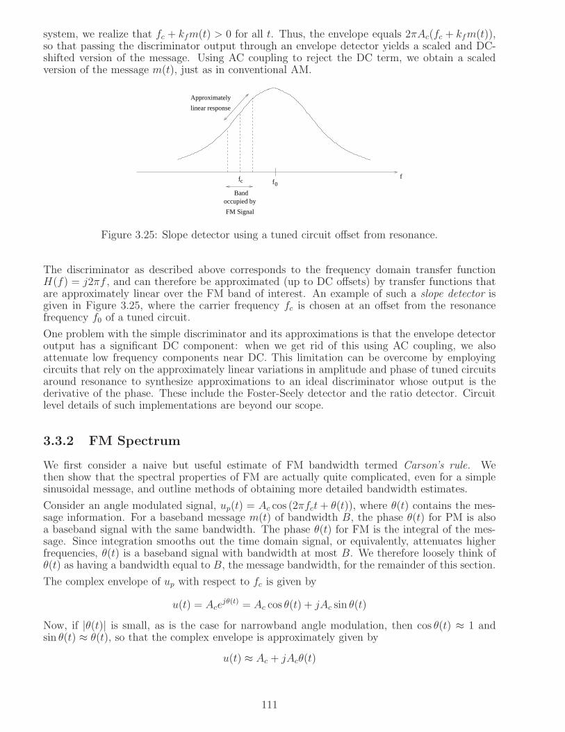
system, we realize that fc + kfm(t) > 0 for all t. Thus, the envelope equals 2πAc(fc + kfm(t)),so that passing the discriminator output through an envelope detector yields a scaled and DC-shifted version of the message. Using AC coupling to reject the DC term, we obtain a scaledversion of the message m(t), just as in conventional AM.

ff0

fc

Bandoccupied by

FM Signal

linear response

Approximately

Figure 3.25: Slope detector using a tuned circuit offset from resonance.

The discriminator as described above corresponds to the frequency domain transfer functionH(f) = j2πf , and can therefore be approximated (up to DC offsets) by transfer functions thatare approximately linear over the FM band of interest. An example of such a slope detector isgiven in Figure 3.25, where the carrier frequency fc is chosen at an offset from the resonancefrequency f0 of a tuned circuit.

One problem with the simple discriminator and its approximations is that the envelope detectoroutput has a significant DC component: when we get rid of this using AC coupling, we alsoattenuate low frequency components near DC. This limitation can be overcome by employingcircuits that rely on the approximately linear variations in amplitude and phase of tuned circuitsaround resonance to synthesize approximations to an ideal discriminator whose output is thederivative of the phase. These include the Foster-Seely detector and the ratio detector. Circuitlevel details of such implementations are beyond our scope.

3.3.2 FM Spectrum

We first consider a naive but useful estimate of FM bandwidth termed Carson’s rule. Wethen show that the spectral properties of FM are actually quite complicated, even for a simplesinusoidal message, and outline methods of obtaining more detailed bandwidth estimates.

Consider an angle modulated signal, up(t) = Ac cos (2πfct+ θ(t)), where θ(t) contains the mes-sage information. For a baseband message m(t) of bandwidth B, the phase θ(t) for PM is alsoa baseband signal with the same bandwidth. The phase θ(t) for FM is the integral of the mes-sage. Since integration smooths out the time domain signal, or equivalently, attenuates higherfrequencies, θ(t) is a baseband signal with bandwidth at most B. We therefore loosely think ofθ(t) as having a bandwidth equal to B, the message bandwidth, for the remainder of this section.

The complex envelope of up with respect to fc is given by

u(t) = Acejθ(t) = Ac cos θ(t) + jAc sin θ(t)

Now, if |θ(t)| is small, as is the case for narrowband angle modulation, then cos θ(t) ≈ 1 andsin θ(t) ≈ θ(t), so that the complex envelope is approximately given by

u(t) ≈ Ac + jAcθ(t)

111

Thus, the passband signal is approximately given by

up(t) ≈ Ac cos 2πfct− θ(t)Ac sin 2πfct

Thus, the I component has a large unmodulated carrier contribution as in conventional AM, butthe message information is now in the Q component instead of in the I component, as in AM.The Fourier transform is given by

Up(f) =Ac

2(δ(f − fc) + δ(f + fc))−

Ac

2j(Θ(f − fc)−Θ(f + fc))

where Θ(f) denotes the Fourier transform of θ(t). The magnitude spectrum is therefore givenby

|Up(f)| =Ac

2(δ(f − fc) + δ(f + fc)) +

Ac

2(|Θ(f − fc)|+ |Θ(f + fc)|) (3.27)

Thus, the bandwidth of a narrowband FM signal is 2B, or twice the message bandwidth, just asin AM. For example, narrowband angle modulation with a sinusoidal message m(t) = cos 2πfmt

occupies a bandwidth of 2fm: θ(t) =kffm

sin 2πfmt for FM, and θ(t) = kp cos 2πfmt) for PM.

For wideband FM, we would expect the bandwidth to be dominated by the frequency deviationkfm(t). For messages that have positive and negative peaks of similar size, the frequency devia-tion ranges between −∆fmax and ∆fmax, where ∆fmax = kfmaxt|m(t)|. In this case, we expectthe bandwidth to be dominated by the instantaneous deviations around the carrier frequency,which spans an interval of length 2∆fmax.

Carson’s rule: This is an estimate for the bandwidth of a general FM signal, based on simplyadding up the estimates from our separate discussion of narrowband and wideband modulation:

BFM ≈ 2B + 2∆fmax = 2B(β + 1) , Carson′s rule (3.28)

where β = ∆fmax/B is the modulation index, also called the FM deviation ratio, defined earlier.

FM Spectrum for a Sinusoidal Message: In order to get more detailed insight into whatthe spectrum of an FM signal looks like, let us now consider the example of a sinusoidal message,for which the phase deviation is given by θ(t) = β sin 2πfmt, from (3.25). The complex envelopeof the FM signal with respect to fc is given by

u(t) = ejθ(t) = ejβ sin 2πfmt

Since the sinusoid in the exponent is periodic with period 1fm

, so is u(t). It can therefore be

expanded into a Fourier series of the form

u(t) =

∞∑

n=−∞u[n]ej2πnfmt

where the Fourier coefficients u[n] are given by

u[n] = fm

∫ 12fm

− 12fm

u(t)e−j2πnfmtdt = fm

∫ 12fm

− 12fm

ejβ sin 2πfmte−j2πnfmtdt

Using the change of variables 2πfmt = x, we have

u[n] =1

2π

∫ π

−π

ej(β sinx−nx)dx = Jn(β)

112

where Jn(·) is the Bessel function of the first kind of order n. While the integrand above iscomplex-valued, the integral is real-valued. To see this, use Euler’s formula:

ej(β sinx−nx) = cos(β sin x− nx) + j sin(β sin x− nx)

Since β sin x−nx and the sine function are both odd, the imaginary term sin(β sin x−nx) aboveis an odd function, and integrates out to zero over [−π, π]. The real part is even, hence theintegral over [−π, π] is simply twice that over [0, π]. We summarize as follows:

u[n] = Jn(β) =1

2π

∫ π

−π

ej(β sinx−nx)dx =1

π

∫ π

0

cos(β sin x− nx)dx (3.29)

0 1 2 3 4 5 6 7 8 9 10−0.5

0

0.5

1

β

J0(β)

J1(β)

J2(β)

J3(β)

Figure 3.26: Bessel functions of the first kind, Jn(β) versus β, for n = 0, 1, 2, 3.

Bessel functions are available in mathematical software packages such as Matlab and Mathemat-ica. Figure 3.26 shows some Bessel function plots. Some properties of Bessel functions worthnoting are as follows:• For n integer, Jn(β) == (−1)nJ−n(β) = (−1)nJn(−β).• For fixed β, Jn(β) tends to zero fast as n gets large, so that the complex envelope is well ap-proximated by a finite number of Fourier series components. In particular, a good approximationis that Jn(β) is small for n > β + 1. This leads to an approximation for the bandwidth of theFM signal given by 2(β + 1)fm, which is consistent with Carson’s rule.• For fixed n, Jn(β) vanishes for specific values of β, a fact that can be used for spectral shaping.

To summarize, the complex envelope of an FM signal modulated by a sinusoidal message can bewritten as

u(t) = ejβ sin 2πfmt =∞∑

n=−∞Jn(β)e

j2πnfmt (3.30)

The corresponding spectrum is given by

U(f) =

∞∑

n=−∞Jn(β)δ(f − nfm) (3.31)

113

Noting that |J−n(β)| = |Jn(β)|, the complex envelope has discrete frequency components at±nfmof strength |Jn(β)|: these correspond to frequency components at fc ± nfm in the passband FMsignal.

Fractional power containment bandwidth: By Parseval’s identity for Fourier series, thepower of the complex envelope is given by

1 = |u(t)|2 = |u(t)|2 =∞∑

n=−∞J2n(β) = J2

0 (β) + 2∞∑

n=1

J2n(β)

we can compute the fractional power containment bandwidth as 2Kfm, where K ≥ 1 is thesmaller integer such that

J20 (β) + 2

K∑

n=1

J2n(β) ≥ α

where α is the desired fraction of power within the band. (e.g., α = 0.99 for the 99% powercontainment bandwidth). For integer values of β = 1, ..., 10, we find that K = β + 1 provides agood approximation to the 99% power containment bandwidth, which is again consistent withCarson’s formula.

3.3.3 Concept synthesis for FM

a(t)

−2 mV

2 mV

t (microsec)100 ...

200

...

Figure 3.27: Input to the VCO in Example 3.3.1.

The following worked problem brings together some of the concepts we have discussed regardingFM.

Example 3.3.1 The signal a(t) shown in Figure 3.27 is fed to a VCO with quiescent frequencyof 5 MHz and frequency deviation of 25 KHz/mV. Denote the output of the VCO by y(t).(a) Provide an estimate of the bandwidth of y. Clearly state the assumptions that you make.(b) The signal y(t) is passed through an ideal bandpass filter of bandwidth 5 KHz, centered at5.005 MHz. Provide the simplest possible expression for the power at the filter output (if youcan give a numerical answer, do so).Solution: (a) The VCO output is an FM signal with

∆fmax = kfmaxtm(t) = 25 KHz/mV × 2 mV = 50 KHz

The message is periodic with period 100 microseconds, hence its fundamental frequency is 10KHz. Approximating its bandwidth by its first harmonic, we have B ≈ 10 KHz. Using Carson’sformula, we can approximate the bandwidth of the FM signal at the VCO output as

BFM ≈ 2∆fmax + 2B ≈ 120 KHz

(b) The complex envelope of the VCO output is given by ejθ(t), where

θ(t) = 2πkf

∫

m(τ)dτ

114

For periodic messages with zero DC value (as is the case for m(t) here), θ(t), and hence, ejθ(t)

has the same period as the message. We can therefore express the complex envelope as a Fourierseries with complex exponentials at frequencies nfm, where fm = 10 KHz is the fundamentalfrequency for the message, and where n takes integer values. Thus, the FM signal has discretecomponents at fc + nfm, where fc = 5 MHz in this example. A bandpass filter at 5.005 MHzwith bandwidth 5 KHz does not capture any of these components, since it spans the interval[5.0025, 5.0075] MHz, whereas the nearest Fourier components are at 5 MHz and 5.01 MHz.Thus, the power at the output of the bandpass filter is zero.

3.4 The Superheterodyne Receiver

The receiver in a radio communication system must downconvert the passband received signaldown to baseband in order to recover the message. At the turn of the twentieth century, itwas difficult to produce amplification at frequencies beyond a few MHz) using the vacuum tubetechnology of that time. However, higher carrier frequencies are desirable because of the largeravailable bandwidths and the smaller antennas required. The invention of the superheterodyne,or superhet, receiver was motivated by these considerations. Basically, the idea is to use sloppydesign for front end filtering of the received radio frequency (RF) signal, and for translating it to alower intermediate frequency (IF). The IF signal is then processed using carefully designed filtersand amplifiers. Subsequently, the IF signal can be converted to baseband in a number of differentways: for example, an envelope detector for AM radio, a phase locked loop or discriminatorfor FM radio, and a coherent quadrature demodulator for digital cellular telephone receivers.While the original motivation for the superheterodyne receiver is no longer strictly applicable(modern analog electronics are capable of providing amplification at the carrier frequencies incommercial use), it is still true that gain is easier to provide at lower frequencies than at higherfrequencies. Furthermore, it becomes possible to closely optimize the processing at a fixed IF(in terms of amplifier and filter design), while permitting a tunable RF front end with morerelaxed specifications, which is important for the design of radios that operate over a widerange of carrier frequencies. For example, the superhet architecture is commonly employed forAM and FM broadcast radio receivers, where the RF front end tunes to the desired station,translating the received signal to a fixed IF. Radio receivers built with discrete components oftentake advantage of the widespread availability of inexpensive filters at certain commonly usedIF frequencies, such as 455 KHz (used for AM radio) and 10.7 MHz (used for FM radio). Ascarrier frequencies scale up to the GHz range (as is the case for modern digital cellular andwireless local area network transceivers), circuit components shrink with the carrier wavelength,and it becomes possible to implement RF amplifiers and filters using integrated circuits. In suchsettings, a direct conversion architecture, in which the passband signal is directly translated tobaseband, becomes increasingly attractive, as discussed later in this section.

The key element in frequency translation is a mixer, which multiplies two input signals. For ourpresent purpose, one of these inputs is a passband received signal A cos(2πfRF t + θ), where theenvelope A(t) and phase θ(t) are baseband signals that contain message information. The secondinput is a local oscillator (LO) signal, which is a locally generated sinusoid cos(2πfLOt) (we setthe LO phase to zero without loss of generality, effectively adopting it as our phase reference).The output of the mixer is therefore given by

A cos(2πfRF t+ θ) cos(2πfLOt) =A

2cos (2π(fRF − fLO)t+ θ) +

A

2cos (2π(fRF + fLO)t+ θ)

Thus, there are two frequency components at the output of the mixer, fRF + fLO and |fRF −fLO| (remember that we only need to talk about positive frequencies when discussing physically

115

realizable signals, due to the conjugate symmetry of the Fourier transform of real-valued timesignals). In the superhet receiver, we set one of these as our IF, typically the difference frequency:fIF = |fRF − fLO|.

Local Oscillator

LNA BPF (RF) BPF (IF)

Mixer Channel selectImage reject

RF signalinto antenna

IF to basebandconversion

Figure 3.28: Generic block diagram for a superhet receiver.

selection

fRF

fRFfLO = + 455 KHz

Antennareceiving

entire AM band

RF AmplifierTunable

TunableLocal Oscillator

Station

MixerIF amplifier(455 KHz)

Envelopedetector

Audioamplifier

To

speaker

Center frequency

Automatic gain control

Figure 3.29: A superhet AM receiver.

For a given RF and a fixed IF, we therefore have two choices of LO frequency when fIF =|fRF − fLO|: fLO = fRF − fIF and fLO = fRF + fIF To continue the discussion, let us considerthe example of AM broadcast radio, which operates over the band from 540 to 1600 KHz, with10 KHz spacing between the carrier frequencies for different stations. The audio message signalis limited to 5 KHz bandwidth, modulated using conventional AM to obtain an RF signal ofbandwidth 10 KHz. Figure 3.29 shows a block diagram for the superhet architecture commonlyused in AM receivers. The RF bandpass filter must be tuned to the carrier frequency for thedesired station, and at the same time, the LO frequency into the mixer must be chosen so thatthe difference frequency equals the IF frequency of 455 KHz. If fLO = fRF + fIF , then theLO frequency ranges from 995 to 2055 KHz, corresponding to an approximately 2-fold variationin tuning range. If fLO = fRF − fIF , then the LO frequency ranges from 85 to 1145 KHz,corresponding to more than 13-fold variation in tuning range. The first choice is thereforepreferred, because it is easier to implement a tunable oscillator over a smaller tuning range.Having fixed the LO frequency, we have a desired signal at fRF = fLO − fIF that leads to acomponent at IF, and potentially an undesired image frequency at fIM = fLO+fIF = fRF +2fIFthat also leads to a component at IF. The job of the RF bandpass filter is to block this imagefrequency. Thus, the filter must let in the desired signal at fRF (so that its bandwidth must belarger than 10 KHz), but severely attenuate the image frequency which is 910 KHz away fromthe center frequency. It is therefore termed an image reject filter. We see that, for the AMbroadcast radio application, a superhet architecture allows us to design the tunable image rejectfilter to somewhat relaxed specifications. However, the image reject filter does let in not onlythe signal from the desired station, but also those from adjacent stations. It is the job of theIF filter, which is tuned to the fixed frequency of 455 KHz, to filter out these adjacent stations.

116

relaxed specs

f IM

= f + fIFLO= f − fIFLO

fRF

Bchannel

2fIF

H (f)RF

f interf

f IF

IF filter must havesharp cutoff to blockinterfering signal

H (f)IF

fLOf

Image frequencygets blocked

BEFORE TRANSLATION TO IF

AFTER TRANSLATION TO IF

Image rejectfilter has

Figure 3.30: The role of image rejection and channel selection in superhet receivers.

For this purpose, we use a highly selective filter at IF with a bandwidth of 10 KHz. Figure 3.30illustrates these design considerations more generally.

Receivers for FM broadcast radio also commonly use a superhet architecture. The FM broadcastband ranges from 88-108 MHz, with carrier frequency separation of 200 KHz between adjacentstations. The IF is chosen at 10.7 MHz, so that the LO is tuned from 98.7 to 118.7 MHz for thechoice fLO = fRF + fIF . The RF filter specifications remain relaxed: it has to let in the desiredsignal of bandwidth 200 KHz, while rejecting an image frequency which is 2fIF = 21.4 MHz awayfrom its center frequency. We discuss the structure of the FM broadcast signal, particularly theway in which stereo FM is transmitted, in more detail in Section 3.6.

Roughly indexing the difficulty of implementing a filter by the ratio of its center frequency to itsbandwidth, or its Q factor, with high Q being more difficult to implement, we have the followingfundamental tradeoff for superhet receivers. If we use a large IF, then the Q needed for theimage reject filter is smaller. On the other hand, the Q needed for the IF filter to reject aninterfering signal whose frequency is near that of the desired signal becomes higher. In moderndigital communication applications, superheterodyne reception with multiple IF stages may beused in order to work around this tradeoff, in order to achieve the desired gain for the signal ofinterest and to attenuate sufficiently interference from other signals, while achieving an adequatedegree of image rejection. Image rejection can be enhanced by employing appropriately designedimage-reject mixer architectures.

Direct conversion receivers: With the trend towards increasing monolithic integration ofdigital communication transceivers for applications such as cellular telephony and wireless localarea networks, the superhet architecture is often being supplanted by direct conversion (or zeroIF) receivers, in which the passband received signal is directly converted down to basebandusing a quadrature mixer at the RF carrier frequency. In this case, the desired signal is itsown image, which removes the necessity for image rejection. Moreover, interfering signals can befiltered out at baseband, often using sophisticated digital signal processing after analog-to-digitalconversion (ADC), provided that there is enough dynamic range in the circuitry to prevent astrong interferer from swamping the desired signal prior to the ADC. In contrast, the high Qbandpass filters required for image rejection and interference suppression in the superhet design

117

must often be implemented off-chip using, for example, surface acoustic wave (SAW) devices,which is bulky and costly. Thus, direct conversion is in some sense the “obvious” thing to do,except that historically, people were unable to make it work, leading to the superhet architectureserving as the default design through most of the twentieth century. A key problem with directconversion is that LO leakage into the RF input of the mixer causes self-mixing, leading to a DCoffset. While a DC offset can be calibrated out, the main problem is that it can saturate theamplifiers following the mixer, thus swamping out the contribution of the weaker received signal.Note that the DC offset due to LO leakage is not a problem with a superhet architecture, sincethe DC term gets filtered out by the passband IF filter. Other problems with direct conversioninclude 1/f noise and susceptibility to second order nonlinearities, but discussion of these issuesis beyond our current scope. However, since the 1990s, integrated circuit designers have managedto overcome these and other obstacles, and direct conversion receivers have become the normfor monolithic implementations of modern digital communication transceivers. These includecellular systems in various licensed bands ranging from 900 MHz to 2 GHz, and WLANs in the2.4 GHz and 5 GHz unlicensed bands.

The insatiable demand for communication bandwidth virtually assures us that we will seek toexploit frequency bands well beyond 5 GHz, and circuit designers will be making informed choicesbetween the superhet and direct conversion architectures for radios at these higher frequencies.For example, the 60 GHz band in the United States has 7 GHz of unlicensed spectrum; thisband is susceptible to oxygen absorption, and is ideally suited for short range (e.g. 10-500meters range) communication both indoors and outdoors. Similarly, the 71-76 GHz and 81-86 GHz bands, which avoid oxygen absorption loss, are available for semi-unlicensed point-to-point “last mile” links. Just as with cellular and WLAN applications in lower frequency bands,we expect that proliferation of applications using these “millimeter (mm) wave” bands wouldrequire low-cost integrated circuit transceiver implementations. Based on the trends at lowerfrequencies, one is tempted to conjecture that initial circuit designs might be based on superhetarchitectures, with direct conversion receivers becoming subsequently more popular as designersbecome more comfortable with working at these higher frequencies. It is interesting to notethat the design experience at lower carrier frequencies does not go to waste; for example, directconversion receivers at, say, 5 GHz, can serve as the IF stage for superhet receivers for mm wavecommunication.

3.5 The Phase Locked Loop

The phase locked loop (PLL) is an effective FM demodulator, but also has a far broader rangeof applications, including frequency synthesis and synchronization. We therefore treat it sepa-rately from our coverage of FM. The PLL provides a canonical example of the use of feedbackfor estimation and synchronization in communication systems, a principle that is employed invariants such as the Costas’ loop and the delay locked loop.

The key idea behind the PLL, depicted in Figure 3.31, is as follows: we would like to lock on tothe phase of the input to the PLL. We compare the phase of the input with that of the output ofa voltage controlled oscillator (VCO) using a phase detector. The difference between the phasesdrives the input of the VCO. If the VCO output is ahead of the PLL input in phase, then wewould like to retard the VCO output phase. If the VCO output is behind the PLL input in phase,we would like to advance the VCO output phase. This is done by using the phase difference tocontrol the VCO input. Typically, rather than using the output of the phase detector directlyfor this purpose, we smooth it out using a loop filter in order to reduce the effect of noise.

Mixer as phase detector: The classical analog realization of the PLL is based on using amixer (i.e., a multiplier) as a phase detector. To see how this works, consider the product of two

118

VCO Output

i

θo

θi θoFunction of phase difference −

PhaseDetector

LoopFilter

VCO

PLL Input

Phase

Phase

θ

Figure 3.31: PLL block diagram.

x(t)

θi θoAvcA sin ( − )1/2fc+ passband (2 ) term

fc θicA πcos (2 t+ )

fc θov−A sin (2 t+ )π

LoopFilter

VCO

PLL Input

VCO Output

Figure 3.32: PLL realization using a mixer as phase detector.

sinusoids whose phases we are trying to align:

cos(2πfct + θ1) cos(2πfct + θ2) =1

2cos(θ1 − θ2) +

1

2cos(4πfct + θ1 + θ2))

The second term on the right-hand side is a passband signal at 2fc which can be filtered outby a lowpass filter. The first term contains the phase difference θ1 − θ2, and is to be used todrive the VCO so that we eventually match the phases. Thus, the first term should be smallwhen we are near a phase match. Since the driving term is the cosine of the phase difference,the phase match condition is θ1 − θ2 = π/2. That is, using a mixer as our phase detector meansthat, when the PLL is locked, the phase at the VCO output is 90 offset from the phase of thePLL input. Now that we know this, we adopt a more convenient notation, changing variablesto define a phase difference whose value at the desired matched state is zero rather than π/2.Let the PLL input be denoted by Ac cos(2πfc + θi(t)), and let the VCO output be denoted byAv cos(2πfc + θo(t) +

π2) = −Av sin(2πfc + θo(t)). The output of the mixer is now given by

−AcAv cos (2πfc + θi(t)) sin (2πfc + θo(t))

= AcAv

2sin (θi(t)− θo(t))− AcAv

2sin (4πfct + θi(t) + θo(t))

The second term on the right-hand side is a passband signal at 2fc which can be filtered outas before. The first term is the desired driving term, and with the change of notation, we notethat the desired state, when the driving term is zero, corresponds to θi = θo. The mixer basedrealization of the PLL is shown in Figure 3.32.

The instantaneous frequency of the VCO is proportional to its input. Thus the phase of theVCO output −sin(2πfct + θo(t)) is given by

θo(t) = Kv

∫ t

0

x(τ)dτ

119

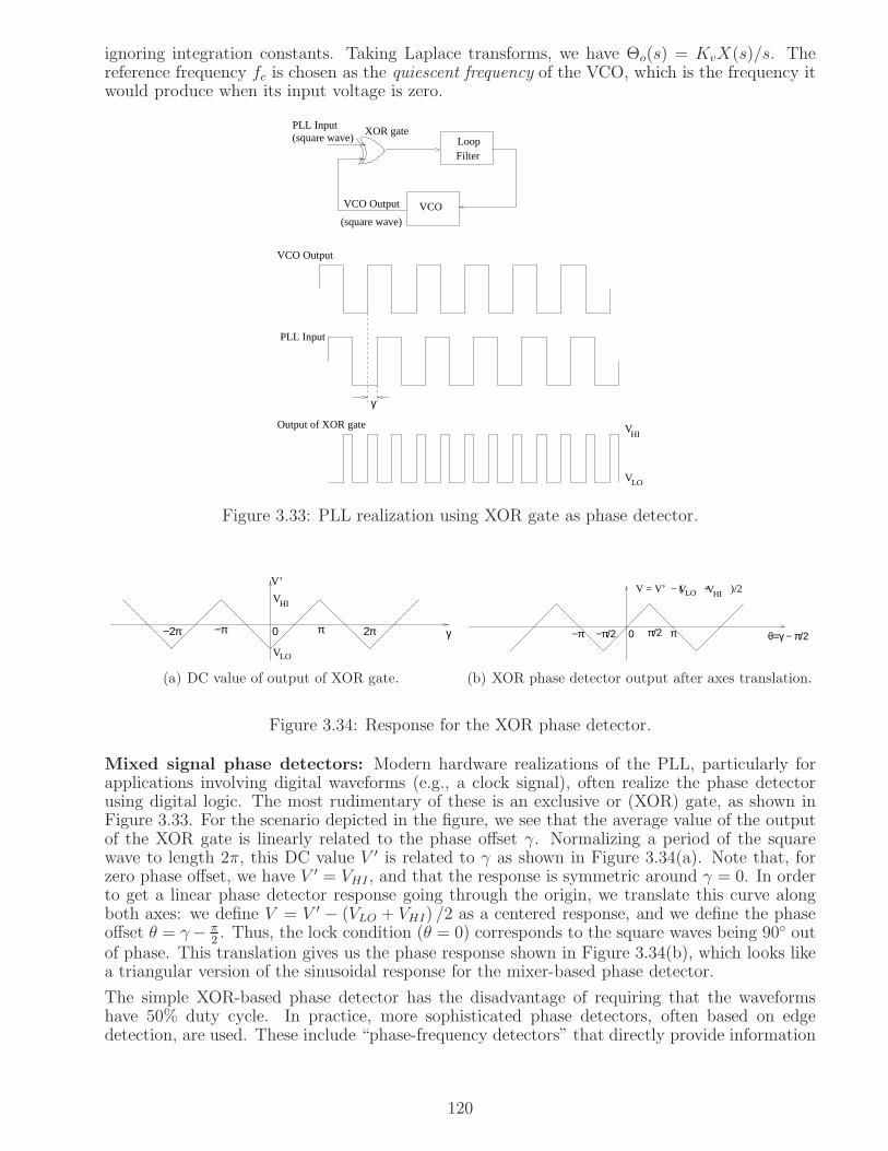
ignoring integration constants. Taking Laplace transforms, we have Θo(s) = KvX(s)/s. Thereference frequency fc is chosen as the quiescent frequency of the VCO, which is the frequency itwould produce when its input voltage is zero.

XOR gate

VHI

VLO

γ

PLL Input

Output of XOR gate

VCO Output

LoopFilter

VCO

PLL Input(square wave)

(square wave)

VCO Output

Figure 3.33: PLL realization using XOR gate as phase detector.

V’

HI

VLO

γπ0 2π−π−2π

V

(a) DC value of output of XOR gate.

−π

LO VHIV = V’ − ( + )/2

θ=γ − π/2π/20−π/2 π

V

(b) XOR phase detector output after axes translation.

Figure 3.34: Response for the XOR phase detector.

Mixed signal phase detectors: Modern hardware realizations of the PLL, particularly forapplications involving digital waveforms (e.g., a clock signal), often realize the phase detectorusing digital logic. The most rudimentary of these is an exclusive or (XOR) gate, as shown inFigure 3.33. For the scenario depicted in the figure, we see that the average value of the outputof the XOR gate is linearly related to the phase offset γ. Normalizing a period of the squarewave to length 2π, this DC value V ′ is related to γ as shown in Figure 3.34(a). Note that, forzero phase offset, we have V ′ = VHI , and that the response is symmetric around γ = 0. In orderto get a linear phase detector response going through the origin, we translate this curve alongboth axes: we define V = V ′ − (VLO + VHI) /2 as a centered response, and we define the phaseoffset θ = γ− π

2. Thus, the lock condition (θ = 0) corresponds to the square waves being 90 out

of phase. This translation gives us the phase response shown in Figure 3.34(b), which looks likea triangular version of the sinusoidal response for the mixer-based phase detector.

The simple XOR-based phase detector has the disadvantage of requiring that the waveformshave 50% duty cycle. In practice, more sophisticated phase detectors, often based on edgedetection, are used. These include “phase-frequency detectors” that directly provide information

120

on frequency differences, which is useful for rapid locking. While discussion of the many phasedetector variants employed in hardware design is beyond our scope, references for further studyare provided at the end of this chapter.

3.5.1 PLL Applications

Before trying to understand how a PLL works in more detail, let us discuss how we would useit, assuming that it has been properly designed. That is, suppose we can design a system suchas that depicted in Figure 3.32, such that θo(t) ≈ θi(t). What would we do with such a system?

Output

i θoFunction of phase difference −

PhaseDetector

LoopFilter

VCO

FM received

signal

FM Demodulator

θ

Figure 3.35: The PLL is an FM demodulator.

PLL as FM demodulator: If the PLL input is an FM signal, its phase is given by

θi(t) = 2πkf

∫ t

0

m(τ)dτ

The VCO output phase is given by

θo(t) = Kv

∫ t

0

x(τ)dτ

If θo ≈ θi, thendθodt

≈ dθidt, so that

Kvx(t) ≈ 2πkfm(t)

That is, the VCO input is approximately equal to a scaled version of the message. Thus, thePLL is an FM demodulator, where the FM signal is the input to the PLL, and the demodulatoroutput is the VCO input, as shown in Figure 3.35.

PLL as frequency synthesizer: The PLL is often used to synthesize the local oscillators usedin communication transmitters and receivers. In a typical scenario, we might have a crystaloscillator which provides an accurate frequency reference at a relatively low frequency, say 40MHz. We wish to use this to derive an accurate frequency reference at a higher frequency, say 1GHz, which might be the local oscillator used at an IF or RF stage in the transceiver. We havea VCO that can produce frequencies around 1 GHz (but is not calibrated to produce the exactvalue of the desired frequency), and we wish to use it to obtain a frequency f0 that is exactlyK times the crystal frequency fcrystal. This can be achieved by adding a frequency divider intothe PLL loop, as shown in Figure 3.36. Such frequency dividers can be implemented digitallyby appropriately skipping pulses. Many variants of this basic concept are possible, such as usingmultiple frequency dividers, frequency multipliers, or multiple interacting loops.

All of these applications rely on the basic property that the VCO output phase successfully trackssome reference phase using the feedback in the loop. Let us now try to get some insight into howthis happens, and into the impact of various parameters on the PLL’s performance.

121

reference

crystal

Kfcrystal

DetectorPhase Loop

Filter

VCO

Frequency Divider

(divide by K)

synthesizerFrequency

output

CrystalOscillator Frequency

f

Figure 3.36: Frequency synthesis using a PLL by inserting a frequency divider into the loop.

3.5.2 Mathematical Model for the PLL

−

o

θisin( ) K G(s)

1/s

VCO functionality(normalized)

Loop gainand filter

θ

Figure 3.37: Nonlinear model for mixer-based PLL.

The mixer-based PLL in Figure 3.32 can be modeled as shown in Figure 3.37, where θi(t) isthe input phase, and θo(t) is the output phase. It is also useful to define the correspondinginstantaneous frequencies (or rather, frequency deviations from the VCO quiescent frequencyfc):

fi(t) =1

2π

dθi(t)

dt, fo(t) =

1

2π

dθo(t)

dt

The phase and frequency errors are defined as

θe(t) = θi(t)− θo(t) , fe(t) = fi(t)− fo(t)

In deriving this model, we can ignore the passband term at 2fc, which will get rejected by theintegration operation due to the VCO, as well as by the loop filter (if a nontrivial lowpass loopfilter is employed). From Figure 3.32, the sine of the phase difference is amplified by 1

2AcAv due

to the amplitudes of the PLL input and VCO output. This is passed through the loop filter,which has transfer function G(s), and then through the VCO, which has a transfer function Kv/s.The loop gain K shown in Figure 3.37 is set to be the product K = 1

2AcAvKv (in addition, the

loop gain also includes additional amplification or attenuation in the loop that is not accountedfor in the transfer function G(s)).

The model in Figure 3.37 is difficult to analyze because of the sin(·) nonlinearity after the phasedifference operation. One way to avoid this difficulty is to linearize the model by simply dropping

122

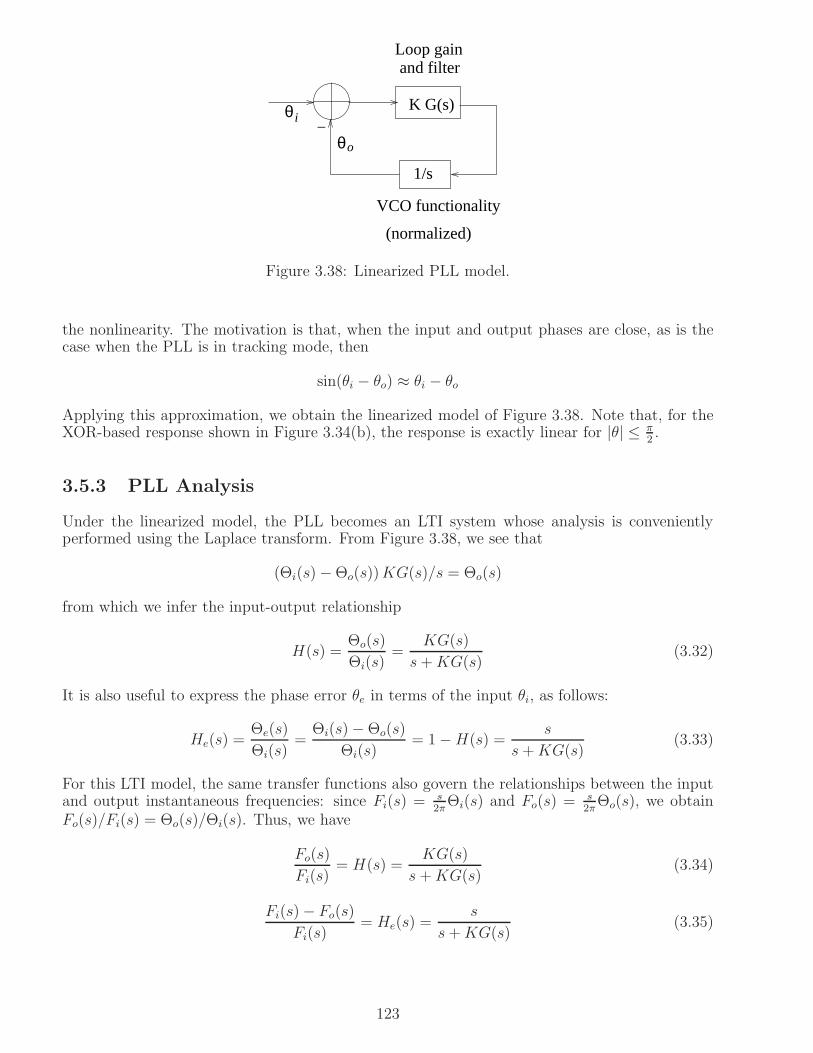
and filter

i

θo

−K G(s)

1/s

(normalized)

VCO functionality

Loop gain

θ

Figure 3.38: Linearized PLL model.

the nonlinearity. The motivation is that, when the input and output phases are close, as is thecase when the PLL is in tracking mode, then

sin(θi − θo) ≈ θi − θo

Applying this approximation, we obtain the linearized model of Figure 3.38. Note that, for theXOR-based response shown in Figure 3.34(b), the response is exactly linear for |θ| ≤ π

2.

3.5.3 PLL Analysis

Under the linearized model, the PLL becomes an LTI system whose analysis is convenientlyperformed using the Laplace transform. From Figure 3.38, we see that

(Θi(s)−Θo(s))KG(s)/s = Θo(s)

from which we infer the input-output relationship

H(s) =Θo(s)

Θi(s)=

KG(s)

s+KG(s)(3.32)

It is also useful to express the phase error θe in terms of the input θi, as follows:

He(s) =Θe(s)

Θi(s)=

Θi(s)−Θo(s)

Θi(s)= 1−H(s) =

s

s+KG(s)(3.33)

For this LTI model, the same transfer functions also govern the relationships between the inputand output instantaneous frequencies: since Fi(s) = s

2πΘi(s) and Fo(s) = s

2πΘo(s), we obtain

Fo(s)/Fi(s) = Θo(s)/Θi(s). Thus, we have

Fo(s)

Fi(s)= H(s) =

KG(s)

s +KG(s)(3.34)

Fi(s)− Fo(s)

Fi(s)= He(s) =

s

s+KG(s)(3.35)

123

First order PLL: When we have a trivial loop filter, G(s) = 1, we obtain the first order response

H(s) =K

s+K, He(s) =

s

s+K

which is a stable response for loop gain K > 0, with a single pole at s = −K. It is interesting tosee what happens when the input phase is a step function, θi(t) = ∆θI[0,∞)(t), or Θi(s) = ∆θ/s.We obtain

Θo(s) = H(s)Θi(s) =K∆θ

s(s+K)=

∆θ

s− ∆θ

s+K

Taking the inverse Laplace transform, we obtain

θo(t) = ∆θ(1− e−Kt)I[0,∞)(t)

so that θo(t) → ∆θ as t → ∞. Thus, the first order PLL can track a sudden change in phase,with the output phase converging to the input phase exponentially fast. The residual phase erroris zero. Note that we could also have inferred this quickly from the final value theorem, withouttaking the inverse Laplace transform:

limt→∞

θe(t) = lims→0

sΘe(s) = lims→0

sHe(s)Θi(s) (3.36)

Specializing to the setting of interest, we obtain

limt→∞

θe(t) = lims→0

ss

s+K

∆θ0s

= 0

We now examine the response of the first order PLL to a frequency step ∆f , so that the instanta-neous input frequency is fi(t) = ∆fI[0,∞)(t). The corresponding Laplace transform is Fi(s) =

∆fs.

The input phase is the integral of the instantaneous frequency:

θi(t) = 2π

∫ t

0

fi(τ)dτ

The Laplace transform of the input phase is therefore given by

Θi(s) = 2πF (s)/s =2π∆f

s2

Given that the input-output relationships are identical for frequency and phase, we can reusethe computations we did for the phase step input, replacing phase by frequency, to conclude thatfo(t) = ∆f(1− e−Kt)I[0,∞)(t) → ∆f as t → ∞, so that the steady-state frequency error is zero.The corresponding output phase trajectory is left as an exercise, but we can use the final valuetheorem to compute the limiting value of the phase error:

limt→∞

θe(t) = lims→0

ss

s+K

2π∆f

s2=

2π∆f

K

Thus, the first order PLL can adapt its frequency to track a step frequency change, but there isa nonzero steady-state phase error. This can be fixed by increasing the order of the PLL, as wenow show below.

Second order PLL: We now introduce a loop filter which feeds back both the phase error andthe integral of the phase error to the VCO input (in control theory terminology, we are using

124

”proportional plus integral” feedback). That is, G(s) = 1 + a/s, where a > 0. This yields thesecond order response

H(s) =KG(s)

s+KG(s)=

K(s+ a)

s2 +Ks+Ka

He(s) =s

s+KG(s)=

s2

s2 +Ks +Ka

The poles of the response are at s = −K±√K2−4Ka2

. It is easy to check that the response is stable(i.e., the poles are in the left half plane) for K > 0. The poles are conjugate symmetric with animaginary component if K2 − 4Ka < 0, or K < 4a, otherwise they are both real-valued. Notethat the phase error due to a step frequency response does go to zero. This is easily seen byinvoking the final value theorem (3.36):

limt→∞

θe(t) = lims→0

ss2

s2 +Ks+Ka

2π∆f

s2= 0

Thus, the second order PLL has zero steady state frequency and phase errors when respondingto a constant frequency offset.

We have seen now that the first order PLL can handle step phase changes, and the second orderPLL can handle step frequency changes, while driving the steady-state phase error to zero. Thispattern continues as we keep increasing the order of the PLL: for example, a third order PLLcan handle a linear frequency ramp, which corresponds to Θi(s) being proportional to 1/s3.

Linearized analysis provides quick insight into the complexity of the phase/frequency variationsthat the PLL can track, as a function of the choice of loop filter and loop gain. We now takeanother look at the first order PLL, accounting for the sin(·) nonlinearity in Figure 3.37, inorder to provide a glimpse of the approach used for handling the nonlinear differential equationsinvolved, and to compare the results with the linearized analysis.

Nonlinear model for the first order PLL: Let us try to express the phase error θe in terms ofthe input phase for a first order PLL, with G(s) = 1. The model of Figure 3.37 can be expressedin the time domain as:

∫ t

0

K sin(θe(τ))dτ = θo(t) = θi(t)− θe(t)

Differentiating with respect to t, we obtain

K sin θe =dθidt

− dθedt

(3.37)

(Both θe and θi are functions of t, but we suppress the dependence for notational simplicity.)Let us now specialize to the specific example of a step frequency input, for which

dθidt

= 2π∆f

Plugging into (3.37) and rearranging, we get

dθedt

= 2π∆f −K sin θe (3.38)

We cannot solve the nonlinear differential equation (3.38) for θe analytically, but we can getuseful insight by a “phase plane plot” of dθe

dtagainst θe, as shown in Figure 3.39. Since sin θe ≤ 1,

we have dθedt

≥ 2π∆f − K, so that, if ∆f > K2π, then dθe

dt> 0 for all t. Thus, for large enough

125

PLL locks

2π∆f − K

2π∆f

θe

θe(0) θe(1)

θed /dt

θe

2π∆f

2π∆f − K

θed /dtPLL does not lock

Figure 3.39: Phase plane plot for first order PLL.

frequency offset, the loop never locks. On the other hand, if ∆f < K2π, then the loop does lock.

In this case, starting from an initial error, say θe(0), the phase error follows the trajectory to theright (if the derivative is positive) or left (if the derivative is negative) until it hits a point atwhich dθe

dt= 0. From (3.38), this happens when

sin θe =2π∆f

K(3.39)

Due to the periodicity of the sine function, if θ is a solution to the preceding equation, so isθ + 2π. Thus, if the equation has a solution, there must be at least one solution in the basicinterval [−π, π]. Moreover, since sin θ = sin(π − θ), if θ is a solution, so is π − θ, so that thereare actually two solutions in [−π, π]. Let us denote by θe(0) = sin−1

(

2π∆fK

)

the solution thatlies in the interval [−π/2, π/2]. This forms a stable equilibrium: from (3.38), we see that thederivative is negative for phase error slightly above θe(0), and is positive as the phase errorslightly below θe(0), so that the phase error is driven back to θe(0) in each case. Using exactlythe same argument, we see that the points θe(0) + 2nπ are also stable equilibria, where n takesinteger values. However, another solution to (3.39) is θe(1) = π − θ(0), and translations of itby . It is easy to see that this is an unstable equilibrium: when there is a slight perturbation,the sign of the derivative is such that it drives the phase error away from θe(1). In general,θe(1) + 2nπ are unstable equlibria, where n takes integer values. Thus, if the frequency offset iswithin the “pull-in range” K

2πof the first order PLL, then the steady state phase offset (modulo

2π) is θe(0) = sin−1(

2π∆fK

)

, which, for small values of 2π∆fK

, is approximately equal to the value2π∆fK

predicted by the linearized analysis.

Linear versus nonlinear model: Roughly speaking, the nonlinear model (which we simplysimulate when phase-plane plots get too complicated) tells us when the PLL locks, while the

126

linearized analysis provides accurate estimates when the PLL does lock. The linearized modelalso tells us something about scenarios when the PLL does not lock: when the phase error blowsup for the linearized model, it indicates that the PLL will perform poorly. This is because thelinearized model holds under the assumption that the phase error is small; if the phase errorunder this optimistic assumption turns out not to be small, then our initial assumption musthave been wrong, and the phase error must be large.

PLL Input Phase Detector(0.5 V/radian)

VCO(10 KHz/V)

Figure 3.40: PLL for Example 3.5.1.

The following worked problem illustrates application of linearized PLL analysis.

Example 3.5.1 Consider the PLL shown in Figure 3.40, assumed to be locked at time zero.(a) Suppose that the input phase jumps by e = 2.72 radians at time zero (set the phase justbefore the jump to zero, without loss of generality). How long does it take for the differencebetween the PLL input phase and VCO output phase to shrink to 1 radian? (Make sure youspecify the unit of time that you use.)(b) Find the limiting value of the phase error (in radians) if the frequency jumps by 1 KHz justafter time zero.Solution: Let θe(t) = θi(t) − θo(t) denote the phase error. In the s domain, it is related to theinput phase as follows:

Θi(s)−K

sΘe(s) = Θe(s)

so thatΘe(s)

Θi(s)=

s

s+K

(a) For a phase jump of e radians at time zero, we have Θi(s) =es, which yields

Θe(s) = Θi(s)s

s+K=

e

s+K

Going to the time domain, we have

θe(t) = ee−Kt = e1−Kt

so that θe(t) = 1 for 1−Kt = 0, or t = 1K

= 15milliseconds.

(b) For a frequency jump of ∆f , the Laplace transform of the input phase is given by

Θi(s) =2π∆f

s2

so that the phase error is given by

Θe(s) = Θi(s)s

s+K=

2π∆f

s(s+K)

127

Using the final value theorem, we have

limt→∞

θe(t) = lims→0

sΘe(s) =2π∆f

K

For ∆f = 1 KHz and K = 5 KHz/radian, this yields a phase error of 2π/5 radians, or 72.

3.6 Some Analog Communication Systems

Some of the analog communication systems that we encounter (or at least, used to encounter)in our daily lives include broadcast radio and television. We have already discussed AM radio inthe context of the superhet receiver. We now briefly discuss FM radio and television. Our goalis to highlight design concepts, and the role played in these systems by the various modulationformats we have studied, rather than to provide a detailed technical description. Other commonlyencountered examples of analog communication that we do not discuss include analog storagemedia (audiotapes and videotapes), analog wireline telephony, analog cellular telephony, amateurham radio, and wireless microphones.

3.6.1 FM radio

L+R signal

533815 19 23 Frequency (KHz)

Pilot

DSB−SC modulatedL−R signal

Figure 3.41: Spectrum of baseband input to FM modulator for FM stereo broadcast.

FM mono radio employs a peak frequency deviation of 75 KHz, with the baseband audio messagesignal bandlimited to 15 KHz; this corresponds to a modulation index of 5. Using Carson’sformula, the bandwidth of the FM radio signal can be estimated as 180 KHz. The separationbetween adjacent radio stations is 200 KHz. FM stereo broadcast transmits two audio channels,“left” and “right,” in a manner that is backwards compatible with mono broadcast, in thata standard mono receiver can extract the sum of the left and right channels, while remainingoblivious to whether the broadcast signal is mono or stereo. The structure of the baseband signalinto the FM modulator is shown in Figure 3.41. The sum of the left and right channels, or theL+R signal, occupies a band from 30 Hz to 15 KHz. The difference, or the L−R signal (whichalso has a bandwidth of 15 KHz), is modulated using DSB-SC, using a carrier frequency of 38KHz, and hence occupies a band from 23 KHz to 53 KHz. A pilot tone at 19 KHz, at half thecarrier frequency for the DSB signal, is provided to enable coherent demodulation of the DSB-SCsignal. The spacing between adjacent FM stereo broadcast stations is still 200 KHz, which makesit a somewhat tight fit (if we apply Carson’s formula with a maximum frequency deviation of 75KHz, we obtain an RF bandwidth of 256 KHz).

The format of the baseband signal in Figure 3.41 (in particular, the DSB-SC modulation of thedifference signal) seems rather contrived, but the corresponding modulator can be implementedquite simply, as sketched in Figure 3.42: we simply switch between the L and R channel audiosignals using a 38 KHz clock. As we shown in one of the problems, this directly yields the L+R

128

signal

38 KHz clock

R channel signal

L channel signal

Frequency divideby two

FM modulatorTransmitted

signal

19 KHz pilot

Compositemessage

Figure 3.42: Block diagram of a simple FM stereo transmitter.

signal, plus the DSB-SC modulated L− R signal. It remains to add in the 19 KHz pilot beforefeeding the composite baseband signal to the FM modulator.

The receiver employs an FM demodulator to obtain an estimate of the baseband transmittedsignal. The L + R signal is obtained by bandlimiting the output of the FM demodulator to 15KHz using a lowpass filter; this is what an oblivious mono receiver would do. A stereo receiver,in addition, processes the output of the FM demodulator in the band from 15 KHz to 53 KHz.It extracts the 19 KHz pilot tone, doubles its frequency to obtain a coherent carrier reference,and uses that to demodulate the L− R signal sent using DSB-SC. It then obtains the L and Rchannels by adding and subtracting the L+R and L− R signals from each other, respectively.

3.6.2 Analog broadcast TV

While analog broadcast TV is obsolete, and is being replaced by digital TV as we speak, wediscuss it briefly here to highlight a few features. First, it illustrates an application of severalmodulation schemes: VSB (for intensity information), quadrature modulation (for the color in-formation), and FM (for audio information). Second, it is an interesting example of how theembedding of different kinds of information in analog form must account for the characteris-tics of the information source (video) and destination (a cathode ray tube TV monitor). Thiscustomized, and rather painful, design process is in contrast to the generality and conceptualsimplification provided by the source-channel separation principle in digital communication (men-tioned in Chapter 1). Indeed, from Chapter 4 onwards, where we restrict attention to digitalcommunication, we do not need to discuss source characteristics.

We first need a quick discussion of CRT TV monitors. An electron beam impinging on a fluores-cent screen is used to emit the light that we perceive as the image on the TV. The electron beamis “raster scanned” in horizontal lines moving down the screen, with its horizontal and verticallocation controlled by two magnetic fields created by voltages, as shown in Figure 3.43. We relyon the persistence of human vision to piece together these discrete scans into a continuous imagein space and time. Black and white TV monitors use a phosphor (or fluorescent material) thatemits white light when struck by electrons. Color TV monitors use three kinds of phosphors,typically arranged as dots on the screen, which emit red, green and blue light, respectively, whenstruck by electrons. Three electron beams are used, one for each color. The intensity of theemitted light is controlled by the intensity of the electron beam. For historical reasons, the scanrate is chosen to be equal to the frequency of the AC power (otherwise, for the power suppliesused at the time, rolling bars would appear on the TV screen). In the United States, this meansthat the scan rate is set at 60 Hz (the frequency of the AC mains).

In order to enable the TV receiver to control the operation of the CRTmonitor, the received signalmust contain not only intensity and color information, but also the timing information requiredto correctly implement the raster scan. Figure 3.44 shows the format of the composite video signal

129

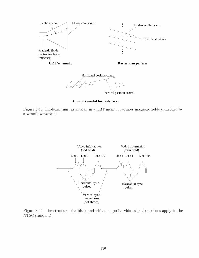
Controls needed for raster scan

Electron beam Fluorescent screen

Magnetic fieldscontrolling beamtrajectory

Horizontal line scan

Horizontal retrace

Horizontal position control

Vertical position control

CRT Schematic Raster scan pattern

Figure 3.43: Implementing raster scan in a CRT monitor requires magnetic fields controlled bysawtooth waveforms.

(even field)

Line 2 Line 4Line 1 Line 3 Line 479 Line 480

Vertical sync

(not shown)waveforms

Horizontal sync pulses

Horizontal syncpulses

Video information Video information(odd field)

Figure 3.44: The structure of a black and white composite video signal (numbers apply to theNTSC standard).

130

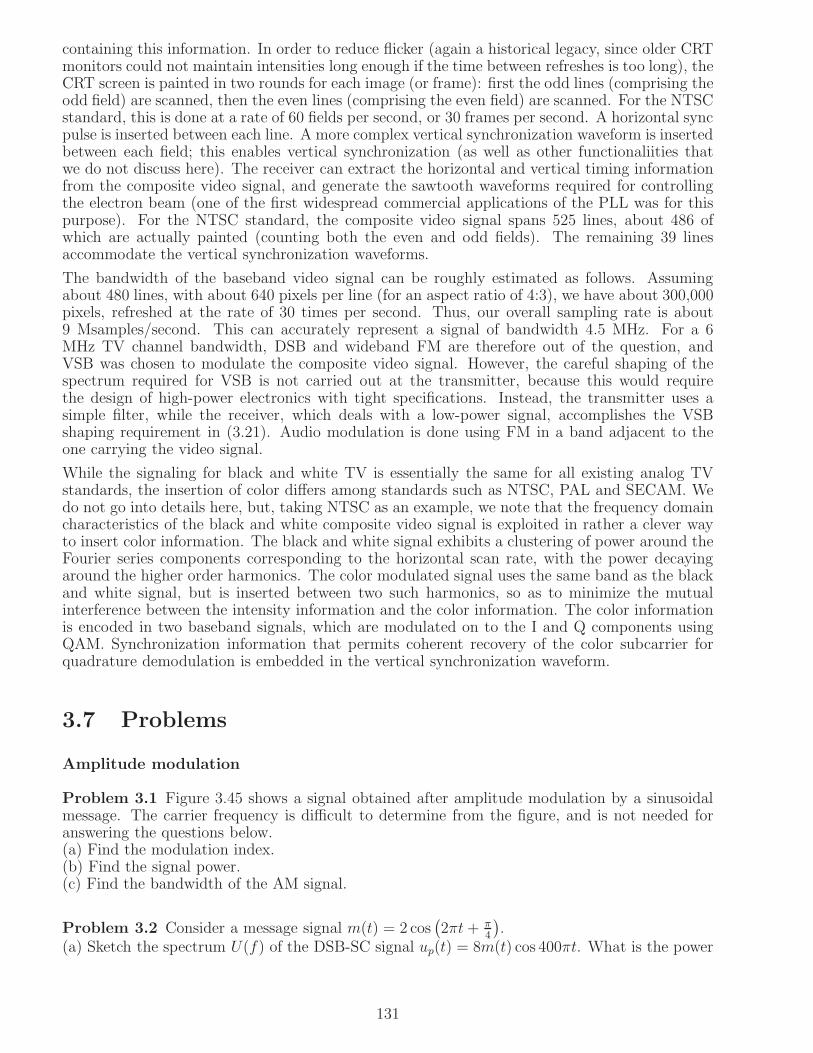
containing this information. In order to reduce flicker (again a historical legacy, since older CRTmonitors could not maintain intensities long enough if the time between refreshes is too long), theCRT screen is painted in two rounds for each image (or frame): first the odd lines (comprising theodd field) are scanned, then the even lines (comprising the even field) are scanned. For the NTSCstandard, this is done at a rate of 60 fields per second, or 30 frames per second. A horizontal syncpulse is inserted between each line. A more complex vertical synchronization waveform is insertedbetween each field; this enables vertical synchronization (as well as other functionaliities thatwe do not discuss here). The receiver can extract the horizontal and vertical timing informationfrom the composite video signal, and generate the sawtooth waveforms required for controllingthe electron beam (one of the first widespread commercial applications of the PLL was for thispurpose). For the NTSC standard, the composite video signal spans 525 lines, about 486 ofwhich are actually painted (counting both the even and odd fields). The remaining 39 linesaccommodate the vertical synchronization waveforms.

The bandwidth of the baseband video signal can be roughly estimated as follows. Assumingabout 480 lines, with about 640 pixels per line (for an aspect ratio of 4:3), we have about 300,000pixels, refreshed at the rate of 30 times per second. Thus, our overall sampling rate is about9 Msamples/second. This can accurately represent a signal of bandwidth 4.5 MHz. For a 6MHz TV channel bandwidth, DSB and wideband FM are therefore out of the question, andVSB was chosen to modulate the composite video signal. However, the careful shaping of thespectrum required for VSB is not carried out at the transmitter, because this would requirethe design of high-power electronics with tight specifications. Instead, the transmitter uses asimple filter, while the receiver, which deals with a low-power signal, accomplishes the VSBshaping requirement in (3.21). Audio modulation is done using FM in a band adjacent to theone carrying the video signal.

While the signaling for black and white TV is essentially the same for all existing analog TVstandards, the insertion of color differs among standards such as NTSC, PAL and SECAM. Wedo not go into details here, but, taking NTSC as an example, we note that the frequency domaincharacteristics of the black and white composite video signal is exploited in rather a clever wayto insert color information. The black and white signal exhibits a clustering of power around theFourier series components corresponding to the horizontal scan rate, with the power decayingaround the higher order harmonics. The color modulated signal uses the same band as the blackand white signal, but is inserted between two such harmonics, so as to minimize the mutualinterference between the intensity information and the color information. The color informationis encoded in two baseband signals, which are modulated on to the I and Q components usingQAM. Synchronization information that permits coherent recovery of the color subcarrier forquadrature demodulation is embedded in the vertical synchronization waveform.

3.7 Problems

Amplitude modulation

Problem 3.1 Figure 3.45 shows a signal obtained after amplitude modulation by a sinusoidalmessage. The carrier frequency is difficult to determine from the figure, and is not needed foranswering the questions below.(a) Find the modulation index.(b) Find the signal power.(c) Find the bandwidth of the AM signal.

Problem 3.2 Consider a message signal m(t) = 2 cos(

2πt+ π4

)

.(a) Sketch the spectrum U(f) of the DSB-SC signal up(t) = 8m(t) cos 400πt. What is the power

131

0 0.2 0.4 0.6 0.8 1 1.2 1.4 1.6 1.8 2−30

−20

−10

0

10

20

30

Time (milliseconds)

Figure 3.45: Amplitude modulated signal for Problem 3.1.

of u?(b) Carefully sketch the output of an ideal envelope detector with input up. On the same plot,sketch the message signal m(t).(c) Let vp(t) denote the waveform obtained by high-pass filtering the signal u(t) so as to letthrough only frequencies above 200 Hz. Find vc(t) and vs(t) such that we can write

vp(t) = vc(t) cos 400πt− vs(t) sin 400πt

and sketch the envelope of v.

Problem 3.3 A message to be transmitted using AM is given by

m(t) = 3 cos 2πt+ 4 sin 6πt

where the unit of time is milliseconds. It is to be sent using a carrier frequency of 600 KHz.(a) What is the message bandwidth? Sketch its magnitude spectrum, clearly specifying the unitsused on the frequency axis.(b) Find an expression for the normalized message mn(t).(c) For a modulation index of 50%, write an explicit time domain expression for the AM signal.(d) What is the power efficiency of the AM signal?(e) Sketch the magnitude spectrum for the AM signal, again clearly specifying the units used onthe frequency axis.(f) The AM signal is to be detected using an envelope detector (as shown in Figure 3.8), withR = 50 ohms. What is a good range of choices for the capacitance C?

Problem 3.4 Consider a message signal m(t) = cos(2πfmt + φ), and a corresponding DSB-SCsignal up(t) = Am(t) cos 2πfct, where fc > fm.(a) Sketch the spectra of the corresponding LSB and USB signals (if the spectrum is complex-valued, sketch the real and imaginary parts separately).(b) Find explicit time domain expressions for the LSB and USB signals.

Problem 3.5 One way of avoiding the use of a mixer in generating AM is to pass x(t) =m(t) + α cos 2πfct through a memoryless nonlinearity and then a bandpass filter.(a) Suppose that M(f) = (1 − |f |/10)I[−10,10] (the unit of frequency is in KHz) and fc is 900

132

KHz. For a nonlinearity f(x) = βx2 + x, sketch the magnitude spectrum at the output of thenonlinearity when the input is x(t), carefully labeling the frequency axis.(b) For the specific settings in (a), characterize the bandpass filter that you should use at theoutput of the nonlinearity so as to generate an AM signal carrying the message m(t)? That is,describe the set of the frequencies that the BPF must reject, and those that it must pass.

Problem 3.6 Consider a DSB signal corresponding to the message m(t) = sinc(2t) and a carrierfrequency fc which is 100 times larger than the message bandwidth, where the unit of time ismilliseconds.(a) Sketch the magnitude spectrum of the DSB signal 10m(t) cos 2πfct, specifying the units onthe frequency axis.(b) Specify a time domain expression for the corresponding LSB signal.(c) Now, suppose that the DSB signal is passed through a bandpass filter whose transfer functionis given by

Hp(f) = (f − fc +1

2)I[fc− 1

2,fc+

12] + I[fc+ 1

2,fc+

32] , f > 0

Sketch the magnitude spectrum of the corresponding VSB signal.(d) Find a time domain expression for the VSB signal of the form

uc(t) cos 2πfct− us(t) sin 2πfct

carefully specifying uc and us. the I and Q components.

waveform

Lowpassfilter

Lowpassfilter

cos 2 f tπ 2

πsin 2 f t2π 1sin 2 f t

cos 2 f tπ 1

_+

Message

waveform

Output

Figure 3.46: Block diagram of Weaver’s SSB modulator for Problem 3.7.

Problem 3.7 Figure 3.46 shows a block diagram of Weaver’s SSB modulator, which works if wechoose f1, f2 and the bandwidth of the lowpass filter appropriately. Let us work through thesechoices for a waveform of the form m(t) = AL cos(2πfLt + φL) + AH cos(2πfHt + φH), wherefH > fL (the design choices we obtain will work for any message whose spectrum lies in the band[fL, fH ].(a) For f1 = (fL+fH)/2 (i.e., choosing the first LO frequency to be in the middle of the messageband), find the time domain waveforms at the outputs of the upper and lower branches after thefirst mixer.(b) Choose the bandwidth of the lowpass filter to be W = fH+2fL

2(assume the lowpass filter is

ideal). Find the time domain waveforms at the outputs of the upper and lower branches afterthe LPF.(c) Now, assuming that f2 ≫ fH , find a time domain expression for the output waveform, as-suming that the upper and lower branches are added together. Is this an LSB or USB waveform?What is the carrier frequency?

133

(d) Repeat (c) when the lower branch is subtracted from the upper branch.Remark: Weaver’s modulator does not require bandpass filters with sharp cutoffs, unlike thedirect approach to generating SSB waveforms by filtering DSB-SC waveforms. It is also simplerthan the Hilbert transform method (the latter requires implementation of a π/2 phase shift overthe entire message band).

920

p

1

f (MHz)880 900

H (f)

Figure 3.47: Bandpass filter for Problem 3.8.

Problem 3.8 Consider the AM signal up(t) = 2(10 + cos 2πfmt) cos 2πfct, where the messagefrequency fm is 1 MHz and the carrier frequency fc is 885 MHz.(a) Suppose that we use superheterodyne reception with an IF of 10.7 MHz, and envelope detec-tion after the IF filter. Envelope detection is accomplished as in Figure 3.8, using a diode andan RC circuit. What would be a good choice of C if R = 100 ohms?(b) The AM signal up(t) is passed through the bandpass filter with transfer function Hp(f) de-picted (for positive frequencies) in Figure 3.47. Find the I and Q components of the filter outputwith respect to reference frequency fc of 885 MHz. Does the filter output represent a form ofmodulation you are familiar with?

Problem 3.9 Consider a message signal m(t) with spectrum M(f) = I[−2,2](f).(a) Sketch the spectrum of the DSB-SC signal uDSB−SC = 10m(t) cos 300πt. What is the powerand bandwidth of u?(b) The signal in (a) is passed through an envelope detector. Sketch the output, and commenton how it is related to the message.(c) What is the smallest value of A such that the message can be recovered without distortionfrom the AM signal uAM = (A+m(t)) cos 300πt by envelope detection?(d) Give a time-domain expression of the form


obtained by high-pass filtering the DSB signal in (a) so as to let through only frequencies above150 Hz.(e) Consider a VSB signal constructed by passing the signal in (a) through a passband filter withtransfer function for positive frequencies specified by:

Hp(f) =

f − 149 149 ≤ f ≤ 1512 f ≥ 151

(you should be able to sketch Hp(f) for both positive and negative frequencies.) Find a timedomain expression for the VSB signal of the form


134

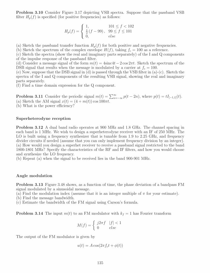
Problem 3.10 Consider Figure 3.17 depicting VSB spectra. Suppose that the passband VSBfilter Hp(f) is specified (for positive frequencies) as follows:

Hp(f) =

1, 101 ≤ f < 10212(f − 99) , 99 ≤ f ≤ 101

0, else

(a) Sketch the passband transfer function Hp(f) for both positive and negative frequencies.(b) Sketch the spectrum of the complex envelope H(f), taking fc = 100 as a reference.(c) Sketch the spectra (show the real and imaginary parts separately) of the I and Q componentsof the impulse response of the passband filter.(d) Consider a message signal of the form m(t) = 4sinc4t−2 cos 2πt. Sketch the spectrum of theDSB signal that results when the message is modulated by a carrier at fc = 100.(e) Now, suppose that the DSB signal in (d) is passed through the VSB filter in (a)-(c). Sketch thespectra of the I and Q components of the resulting VSB signal, showing the real and imaginaryparts separately.(f) Find a time domain expression for the Q component.

Problem 3.11 Consider the periodic signal m(t) =∑∞

n=−∞ p(t− 2n), where p(t) = tI[−1,1](t).(a) Sketch the AM signal x(t) = (4 +m(t)) cos 100πt.(b) What is the power efficiency?

Superheterodyne reception

Problem 3.12 A dual band radio operates at 900 MHz and 1.8 GHz. The channel spacing ineach band is 1 MHz. We wish to design a superheterodyne receiver with an IF of 250 MHz. TheLO is built using a frequency synthesizer that is tunable from 1.9 to 2.25 GHz, and frequencydivider circuits if needed (assume that you can only implement frequency division by an integer).(a) How would you design a superhet receiver to receive a passband signal restricted to the band1800-1801 MHz? Specify the characteristics of the RF and IF filters, and how you would chooseand synthesize the LO frequency.(b) Repeat (a) when the signal to be received lies in the band 900-901 MHz.

Angle modulation

Problem 3.13 Figure 3.48 shows, as a function of time, the phase deviation of a bandpass FMsignal modulated by a sinusoidal message.(a) Find the modulation index (assume that it is an integer multiple of π for your estimate).(b) Find the message bandwidth.(c) Estimate the bandwidth of the FM signal using Carson’s formula.

Problem 3.14 The input m(t) to an FM modulator with kf = 1 has Fourier transform

M(f) =

j2πf |f | < 10 else

The output of the FM modulator is given by

u(t) = A cos(2πfct + φ(t))

135

0 0.1 0.2 0.3 0.4 0.5 0.6 0.7 0.8 0.9 1−600

−400

−200

0

200

400

600

Time (milliseconds)

Pha

se d

evia

tion

(deg

rees

)Figure 3.48: Phase deviation of FM signal for Problem 3.13.

where fc is the carrier frequency.(a) Find an explicit time domain expression for φ(t) and carefully sketch φ(t) as a function oftime.(b) Find the magnitude of the instantaneous frequency deviation from the carrier at time t = 1

4.

(c) Using the result from (b) as an approximation for the maximum frequency deviation, estimatethe bandwidth of u(t).

Problem 3.15 Let p(t) = I[− 12, 12](t) denote a rectangular pulse of unit duration. Construct the

signal

m(t) =

∞∑

n=−∞(−1)np(t− n)

The signal m(t) is input to an FM modulator, whose output is given by

u(t) = 20 cos(2πfct + φ(t))

where

φ(t) = 20π

∫ t

−∞m(τ)dτ + a

and a is chosen such that φ(0) = 0.(a) Carefully sketch both m(t) and φ(t) as a function of time.(b) Approximating the bandwidth of m(t) as W ≈ 2, estimate the bandwidth of u(t) usingCarson’s formula.(c) Suppose that a very narrow ideal BPF (with bandwidth less than 0.1) is placed at fc + α.For which (if any) of the following choices of α will you get nonzero power at the output of theBPF: (i) α = .5, (ii) α = .75, (iii) α = 1.

Problem 3.16 Let u(t) = 20 cos(2000πt+ φ(t)) denote an angle modulated signal.(a) For φ(t) = 0.1 cos 2πt, what is the approximate bandwidth of u?(b) Let y(t) = u12(t). Specify the frequency bands spanned by y(t). In particular, specify theoutput when y is passed through:(i) A BPF centered at 12KHz. Using Carson’s formula, determine the bandwidth of the BPFrequired to recover most of the information in φ from the output.(ii) An ideal LPF of bandwidth 200 Hz.

136

(iii) A BPF of bandwidth 100 Hz centered at 11 KHz.(c) For φ(t) = 2

∑

n s(t− 2n), where s(t) = (1− |t|)I[−1,1].(i) Sketch the instantaneous frequency deviation from the carrier frequency of 1 KHz.(ii) Show that we can write

u(t) =∑

n

cn cos(2000πt+ nαt)

Specify α, and write down an explicit integral expression for cn.

Problem 3.17 Consider the set-up of Problem 3.15, taking the unit of time in milliseconds forconcreteness. You do not need the value of fc, but you can take it to be 1 MHz.(a) Numerically (e.g., using Matlab) compute the Fourier series expansion for the complex enve-lope of the FM waveform, in the same manner as was done for a sinusoidal message. Report themagnitudes of the Fourier series coefficients for the first 5 harmonics.(b) Find the 90%, 95% and 99% power containment bandwidths. Compare with the estimatefrom Carson’s formula obtained in Problem 3.15(b).

Problem 3.18 A VCO with a quiescent frequency of 1 GHz, with a frequency sweep of 2MHz/mV produces an angle modulated signal whose phase deviation θ(t) from a carrier frequencyfc of 1 GHz is shown in Figure 3.49.

VCO

(t)θ

t(microseconds)

10 π

1−1 3−3

πcos(2 f t + (t))θcm(t)2 MHz/mV

Figure 3.49: Set-up for Problem 3.18.

(a) Sketch the input m(t) to the VCO, carefully labeling both the voltage and time axes.(b) Estimate the bandwidth of the angle modulated signal at the VCO output. You may ap-proximate the bandwidth of a periodic signal by that of its first harmonic.

Uncategorized problems

Problem 3.19 The signal m(t) = 2 cos 20πt − cos 40πt, where the unit of time is millisec-onds, and the unit of amplitude is millivolts (mV), is fed to a VCO with quiescent frequencyof 5 MHz and frequency deviation of 100 KHz/mV. Denote the output of the VCO by y(t).(a) Provide an estimate of the bandwidth of y.(b) The signal y(t) is passed through an ideal bandpass filter of bandwidth 5 KHz, centered at5.005 MHz. Describe in detail how you would compute the power at the filter output (if you cancompute the power in closed form, do so).

Problem 3.20 Consider the AM signal up(t) = (A + m(t)) cos 400πt (t in ms) with messagesignal m(t) as in Figure 3.50, where A is 10 mV.(a) If the AM signal is demodulated using an envelope detector with an RC filter, how shouldyou choose C if R = 500 ohms? Try to ensure that the first harmonic (i.e., the fundamental)and the third harmonic of the message are reproduced with minimal distortion.(b) Now, consider an attempt at synchronous demodulation, where the AM signal is downcon-verted using a 201 KHz LO, as shown in Figure 3.51, find and sketch the I and Q components,

137

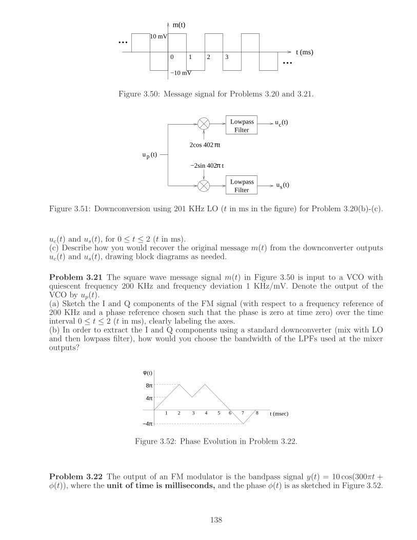
−10 mV

t (ms)

m(t)

2 30 1 ...

... 10 mV

Figure 3.50: Message signal for Problems 3.20 and 3.21.

LowpassFilter

LowpassFilter su (t)

cu (t)

pu (t)

2cos 402 tπ

π−2sin 402 t

Figure 3.51: Downconversion using 201 KHz LO (t in ms in the figure) for Problem 3.20(b)-(c).

uc(t) and us(t), for 0 ≤ t ≤ 2 (t in ms).(c) Describe how you would recover the original message m(t) from the downconverter outputsuc(t) and us(t), drawing block diagrams as needed.

Problem 3.21 The square wave message signal m(t) in Figure 3.50 is input to a VCO withquiescent frequency 200 KHz and frequency deviation 1 KHz/mV. Denote the output of theVCO by up(t).(a) Sketch the I and Q components of the FM signal (with respect to a frequency reference of200 KHz and a phase reference chosen such that the phase is zero at time zero) over the timeinterval 0 ≤ t ≤ 2 (t in ms), clearly labeling the axes.(b) In order to extract the I and Q components using a standard downconverter (mix with LOand then lowpass filter), how would you choose the bandwidth of the LPFs used at the mixeroutputs?

−4π

φ

4 5 6 7 81 2 3 t (msec)

8π

4π

(t)

Figure 3.52: Phase Evolution in Problem 3.22.

Problem 3.22 The output of an FM modulator is the bandpass signal y(t) = 10 cos(300πt +φ(t)), where the unit of time is milliseconds, and the phase φ(t) is as sketched in Figure 3.52.

138

(a) Suppose that y(t) is the output of a VCO with frequency deviation 1 KHz/mV and quiescentfrequency 149 KHz, find and sketch the input to the VCO.(b) Use Carson’s formula to estimate the bandwidth of y(t), clearly stating the approximationsthat you make.

Phase locked loop

Set-up for PLL problems: For the next few problems on PLL modeling and analysis, considerthe linearized model in Figure 3.38, with the following notation: loop filter G(s), loop gain K,and VCO modeled as 1/s. Recall from your background on signals and systems that a secondorder system of the form 1

s2+2ζωns+ω2nis said to have natural frequency ωn (in radians/second)

and damping factor ζ .

Problem 3.23 Let H(s) denote the gain from the PLL input to the output of the VCO. LetHe(s) denote the gain from the PLL input to the input to the loop filter. Let Hm(s) denote thegain from the PLL input to the VCO input.(a) Write down the formulas for H(s), He(s), Hm(s), in terms of K and G(s).(b) Which is the relevant transfer function if the PLL is being used for FM demodulation?(c) Which is the relevant transfer function if the PLL is being used for carrier phase tracking?(d) For G(s) = s+8

sand K = 2, write down expressions for H(s), He(s) and Hm(s). What is the

natural frequency and the damping factor?

Problem 3.24 Suppose the PLL input exhibits a frequency jump of 1 KHz.(a) How would you choose the loop gain K for a first order PLL (G(s) = 1) to ensure a steadystate error of at most 5 degrees?(b) How would you choose the parameters a and K for a second order PLL (G(s) = s+a

s) to have

a natural frequency of 1.414 KHz and a damping factor of 1√2. Specify the units for a and K.

(c) For the parameter choices in (b), find and roughly sketch the phase error as a function oftime for a frequency jump of 1 KHz.

Problem 3.25 Suppose that G(s) = s+16s+4

and K = 4.

(a) Find the transfer function Θo(s)Θi(s)

.

(b) Suppose that the PLL is used for FM demodulation, with the input to the PLL is being anFM signal with instantaneous frequency deviation of the FM signal 10

πm(t), where the message

m(t) = 2 cos t + sin 2t. Using the linearized model for the PLL, find a time domain expressionfor the estimated message provided by the PLL-based demodulator.Hint: What happens to a sinusoid of frequency ω passing through a linear system with transferfunction H(s)?

Problem 3.26 Consider the PLL depicted in Figure 3.53, with input phase φ(t). The outputsignal of interest to us here is v(t), the VCO input. The parameter for the loop filter G(s) isgiven by a = 1000π radians/sec.(a) Assume that the PLL is locked at time 0, and suppose that φ(t) = 1000πtIt>0. Find thelimiting value of v(t).(b) Now, suppose that φ(t) = 4π sin 1000πt. Find an approximate expression for v(t). For fullcredit, simplify as much as possible.(c) For part (b), estimate the bandwidth of the passband signal at the PLL input.

139

G(s) = (s+a)/sPhase Detector1 volt/radian

1KHz/voltVCO

v(t)

Figure 3.53: System for Problem 3.26.

Quiz on analog communication systems

Problem 3.27 Answer the following questions regarding commercial analog communication sys-tems (some of which may no longer exist in your neighborhood).(a) (True or False) The modulation format for analog cellular telephony was conventional AM.(b) (Multiple choice) FM was used in analog TV as follows:(i) to modulate the video signal(ii) to modulate the audio signal(iii) FM was not used in analog TV systems.(c) A superheterodyne receiver for AM radio employs an intermediate frequency (IF) of 455 KHz,and has stations spaced at 10 KHz. Comment briefly on each of the following statements:(i) The AM band is small enough that the problem of image frequencies does not occur.(ii) A bandwidth of 20 KHz for the RF front end is a good choice.(iii) A bandwidth of 20 KHz for the IF filter is a good choice.

140

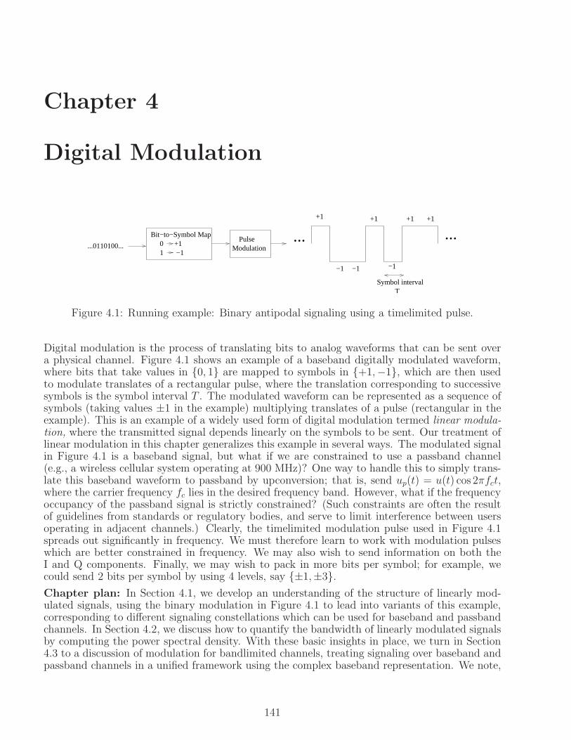
Chapter 4

Digital Modulation

+1

Bit−to−Symbol Map0 +11 −1

...PulseModulation...0110100...

...+1

−1 −1

+1

TSymbol interval

−1

+1

Figure 4.1: Running example: Binary antipodal signaling using a timelimited pulse.

Digital modulation is the process of translating bits to analog waveforms that can be sent overa physical channel. Figure 4.1 shows an example of a baseband digitally modulated waveform,where bits that take values in 0, 1 are mapped to symbols in +1,−1, which are then usedto modulate translates of a rectangular pulse, where the translation corresponding to successivesymbols is the symbol interval T . The modulated waveform can be represented as a sequence ofsymbols (taking values ±1 in the example) multiplying translates of a pulse (rectangular in theexample). This is an example of a widely used form of digital modulation termed linear modula-tion, where the transmitted signal depends linearly on the symbols to be sent. Our treatment oflinear modulation in this chapter generalizes this example in several ways. The modulated signalin Figure 4.1 is a baseband signal, but what if we are constrained to use a passband channel(e.g., a wireless cellular system operating at 900 MHz)? One way to handle this to simply trans-late this baseband waveform to passband by upconversion; that is, send up(t) = u(t) cos 2πfct,where the carrier frequency fc lies in the desired frequency band. However, what if the frequencyoccupancy of the passband signal is strictly constrained? (Such constraints are often the resultof guidelines from standards or regulatory bodies, and serve to limit interference between usersoperating in adjacent channels.) Clearly, the timelimited modulation pulse used in Figure 4.1spreads out significantly in frequency. We must therefore learn to work with modulation pulseswhich are better constrained in frequency. We may also wish to send information on both theI and Q components. Finally, we may wish to pack in more bits per symbol; for example, wecould send 2 bits per symbol by using 4 levels, say ±1,±3.Chapter plan: In Section 4.1, we develop an understanding of the structure of linearly mod-ulated signals, using the binary modulation in Figure 4.1 to lead into variants of this example,corresponding to different signaling constellations which can be used for baseband and passbandchannels. In Section 4.2, we discuss how to quantify the bandwidth of linearly modulated signalsby computing the power spectral density. With these basic insights in place, we turn in Section4.3 to a discussion of modulation for bandlimited channels, treating signaling over baseband andpassband channels in a unified framework using the complex baseband representation. We note,

141

invoking Nyquist’s sampling theorem to determine the degrees of freedom offered by bandlimitedchannels, that linear modulation with a bandlimited modulation pulse can be used to fill all ofthese degrees of freedom. We discuss how to design bandlimited modulation pulses based onthe Nyquist criterion for intersymbol interference (ISI) avoidance. Finally, we discuss orthogonaland biorthogonal modulation in Section 4.4.

Software: Over the course of this and later chapters, we develop a simulation framework forsimulating linear modulation over noisy dispersive channels. Software Lab 4.1 in this chapter isa first step in this direction. Appendix 4.B provides guidance for developing the software for thislab.

4.1 Signal Constellations

0 0.5 1 1.5 2 2.5 3−1

−0.8

−0.6

−0.4

−0.2

0

0.2

0.4

0.6

0.8

1

t/T

Figure 4.2: BPSK illustrated for fc =4Tand symbol sequence +1,−1,−1. The solid line corre-

sponds to the passband signal up(t), and the dashed line to the baseband signal u(t). Note that,due to the change in sign between the first and second symbols, there is a phase discontinuity ofπ at t = T .

The linearly modulated signal depicted in Figure 4.1 can be written in the following generalform:

u(t) =∑

n

b[n]p(t− nT ) (4.1)

where b[n] is a sequence of symbols, and p(t) is the modulating pulse. The symbols take valuesin −1,+1 in our example, and the modulating pulse is a rectangular timelimited pulse. As weproceed along this chapter, we shall see that linear modulation as in (4.1) is far more generallyapplicable, in terms of the set of possible values taken by the symbol sequence, as well as thechoice of modulating pulse.

The modulated waveform (4.1) is a baseband waveform. While it is timelimited in our example,and hence cannot be strictly bandlimited, it is approximately bandlimited to a band around DC.Now, if we are given a passband channel over which to send the information encoded in thiswaveform, one easy approach is to send the passband signal

up(t) = u(t) cos 2πfct (4.2)

where fc is the carrier frequency. That is, the modulated baseband signal is sent as the Icomponent of the passband signal. To see what happens to the passband signal as a consequenceof the modulation, we plot it in Figure 4.2. For the nth symbol interval nT ≤ t < (n + 1)T , wehave up(t) = cos 2πfct if b[n] = +1, and up(t) = − cos 2πfct = cos(2πfct+ π) if b[n] = −1. Thus,binary antipodal modulation switches the phase of the carrier between two values 0 and π, whichis why it is termed Binary Phase Shift Keying (BPSK) when applied to a passband channel:

142

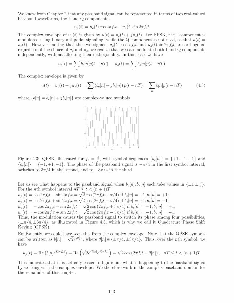
We know from Chapter 2 that any passband signal can be represented in terms of two real-valuedbaseband waveforms, the I and Q components.

up(t) = uc(t) cos 2πfct− us(t) sin 2πfct

The complex envelope of up(t) is given by u(t) = uc(t) + jus(t). For BPSK, the I component ismodulated using binary antipodal signaling, while the Q component is not used, so that u(t) =uc(t). However, noting that the two signals, uc(t) cos 2πfct and us(t) sin 2πfct are orthogonalregardless of the choice of uc and us, we realize that we can modulate both I and Q componentsindependently, without affecting their orthogonality. In this case, we have

uc(t) =∑

n

bc[n]p(t− nT ), us(t) =∑

n

bs[n]p(t− nT )

The complex envelope is given by

u(t) = uc(t) + jus(t) =∑

n

(bc[n] + jbs[n]) p(t− nT ) =∑

n

b[n]p(t− nT ) (4.3)

where b[n] = bc[n] + jbs[n] are complex-valued symbols.

0 0.5 1 1.5 2 2.5 3−1.5

−1

−0.5

0

0.5

1

1.5

t/T

Figure 4.3: QPSK illustrated for fc = 4T, with symbol sequences bc[n] = +1,−1,−1 and

bs[n] = −1,+1,−1. The phase of the passband signal is −π/4 in the first symbol interval,switches to 3π/4 in the second, and to −3π/4 in the third.

Let us see what happens to the passband signal when bc[n], bs[n] each take values in ±1 ± j.For the nth symbol interval nT ≤ t < (n+ 1)T :up(t) = cos 2πfct− sin 2πfct =

√2 cos (2πfct+ π/4) if bc[n] = +1, bs[n] = +1;

up(t) = cos 2πfct + sin 2πfct =√2 cos (2πfct− π/4) if bc[n] = +1, bs[n] = −1;

up(t) = − cos 2πfct− sin 2πfct =√2 cos (2πfct+ 3π/4) if bc[n] = −1, bs[n] = +1;

up(t) = − cos 2πfct + sin 2πfct =√2 cos (2πfct− 3π/4) if bc[n] = −1, bs[n] = −1.

Thus, the modulation causes the passband signal to switch its phase among four possibilities,±π/4,±3π/4, as illustrated in Figure 4.3, which is why we call it Quadrature Phase ShiftKeying (QPSK).

Equivalently, we could have seen this from the complex envelope. Note that the QPSK symbolscan be written as b[n] =

√2ejθ[n], where θ[n]∈ ±π/4,±3π/4. Thus, over the nth symbol, we

have

up(t) = Re(

b[n]ej2πfct)

= Re(√

2ejθ[n]ej2πfct)

=√2 cos (2πfct+ θ[n]) , nT ≤ t < (n + 1)T

This indicates that it is actually easier to figure out what is happening to the passband signalby working with the complex envelope. We therefore work in the complex baseband domain forthe remainder of this chapter.

143

In general, the complex envelope for a linearly modulated signal is given by (4.1), where b[n] =bc[n] + jbs[n] = r[n]ejθ[n] can be complex-valued. We can view this as bc[n] modulating theI component and bs[n] modulating the Q component, or as scaling the envelope by r[n] andswitching the phase by θ[n]. The set of values that each symbol can take is called the signalingalphabet, or constellation. We can plot the constellation in a two-dimensional plot, with the x-axis denoting the real part bc[n] (corresponding to the I component) and the y-axis denoting theimaginary part bs[n] (corresponding to the Q component). Indeed, this is why linear modulationover passband channels is also termed two-dimensional modulation. Note that this provides aunified description of constellations that can be used over both baseband and passband channels:for physical baseband channels, we simply constrain b[n] = bc[n] to be real-valued, setting bs[n] =0.

16QAM

BPSK/2PAM4PAM

QPSK/4PSK/4QAM 8PSK

Figure 4.4: Some commonly used constellations. Note that 2PAM and 4PAM can be used overboth baseband and passband channels, while the two-dimensional constellations QPSK, 8PSKand 16QAM are for use over passband channels.

Figure 4.4 shows some common constellations. Pulse Amplitude Modulation (PAM) correspondsto using multiple amplitude levels along the I component (setting the Q component to zero).This is often used for signaling over physical baseband channels. Using PAM along both I and Qaxes corresponds to Quadrature Amplitude Modulation (QAM). If the constellation points lie ona circle, they only affect the phase of the carrier: such signaling schemes are termed Phase ShiftKeying (PSK). When naming a modulation scheme, we usually indicate the number of pointsin the constellations. BPSK and QPSK are special: BPSK (or 2PSK) can also be classified as2PAM, while QPSK (or 4PSK) can also be classified as 4QAM.

Each symbol in a constellation of size M can be uniquely mapped to log2M bits. For a symbol

rate of 1/T symbols per unit time, the bit rate is therefore log2 MT

bits per unit time. Since thetransmitted bits often contain redundancy due to a channel code employed for error correction ordetection, the information rate is typically smaller than the bit rate. The choice of constellationfor a particular application depends on considerations such as power-bandwidth tradeoffs andimplementation complexity. We shall discuss these issues once we develop more background.

144

4.2 Bandwidth Occupancy

Bandwidth is a precious commodity, hence it is important to quantify the frequency occupancyof communication signals. To this end, consider the complex envelope of a linearly modulatedsignal (the two-sided bandwidth of this complex envelope equals the physical bandwidth of thecorresponding passband signal), which has the form given in (4.1): u(t) =

∑

n b[n]p(t − nT ).The complex-valued symbol sequence b[n] is modeled as random. Modeling the sequence asrandom at the transmitter makes sense because the latter does not control the information beingsent (e.g., it depends on the specific computer file or digital audio signal being sent). Since thisinformation is mapped to the symbols in some fashion, it follows that the symbols themselves arealso random rather than deterministic. Modeling the symbols as random at the receiver makeseven more sense, since the receiver by definition does not know the symbol sequence (otherwisethere would be no need to transmit). However, for characterizing the bandwidth occupancy of thedigitally modulated signal u, we do not compute statistics across different possible realizationsof the symbol sequence b[n]. Rather, we define the quantities of interest in terms of averagesacross time, treating u(t) as a finite power signal which can be modeled as deterministic once thesymbol sequence b[n] is fixed. (We discuss concepts of statistical averaging across realizationslater, when we discuss random processes in Chapter 5.)

We introduce the concept of PSD in Section 4.2.1. In Section 4.2.2, we state our main result onthe PSD of digitally modulated signals, and discuss how to compute bandwidth once we knowthe PSD.

4.2.1 Power Spectral Density

Meter

∆

f∆S ( )x f*

H(f)

x(t)

1

f*

Power

f

Figure 4.5: Operational definition of PSD.

We now introduce the important concept of power spectral density (PSD), which specifies howthe power in a signal is distributed in different frequency bands.

Power Spectral Density: The power spectral density (PSD), Sx(f), for a finite-power signalx(t) is defined through the conceptual measurement depicted in Figure 4.5. Pass x(t) throughan ideal narrowband filter with transfer function

Hf∗(f) =

1, f ∗ − ∆f2< f < f ∗ + ∆f

2

0, else

The PSD evaluated at f ∗, Sx(f∗), is defined as the measured power at the filter output, divided

by the filter width ∆f (in the limit as ∆f → 0).

Example (PSD of complex exponentials): Let us now find the PSD of x(t) = Aej(2πf0t+θ).Since the frequency content of x is concentrated at f0, the power meter in Figure 4.5 will havezero output for f ∗ 6= f0 (as ∆f → 0, f0 falls outside the filter bandwidth for any such f0). Thus,

145

Sx(f) = 0 for f 6= f0. On the other hand, for f ∗ = f0, the output of the power meter is theentire power of x, which is

Px = A2 =

∫ f0+∆f2

f0−∆f2

Sx(f)df

We conclude that the PSD is Sx(f) = A2δ(f−f0). Extending this reasoning to a sum of complexexponentials, we have

PSD of∑

i

Aiej(2πfit+θi) =

∑

i

A2i δ(f − fi)

where fi are distinct frequencies (positive or negative), and Ai, θi are the amplitude and phase,respectively, of the ith complex exponential. Thus, for a real-valued sinusoid, we obtain

Sx(f) =1

4δ(f−f0)+

1

4δ(f +f0) , for x(t) = cos(2πf0t+θ) =

1

2ej(2πf0t+θ)+

1

2e−j(2πf0t+θ) (4.4)

Periodogram-based PSD estimation: One way to carry out the conceptual measurement inFigure 4.5 is to limit x(t) to a finite observation interval, compute its Fourier transform and henceits energy spectral density (which is the magnitude square of the Fourier transform), and thendivide by the length of the observation interval. The PSD is obtained by letting the observationinterval get large. Specifically, define the time-windowed version of x as

xTo(t) = x(t)I[−To2,To

2](t) (4.5)

where To is the length of the observation interval. Since To is finite and x(t) has finite power,xTo(t) has finite energy, and we can compute its Fourier transform

XTo(f) = F(xTo)

The energy spectral density of xTo is given by |XTo(f)|2. Averaging this over the observationinterval, we obtain the estimated PSD

Sx(f) =|XTo(f)|2

To(4.6)

The estimate in (4.6), which is termed a periodogram, can typically be obtained by taking theDFT of a sampled version of the time windowed signal; the time interval To must be large enoughto give the desired frequency resolution, while the sampling rate must be large enough to capturethe variations in x(t). The estimated PSDs obtained over multiple observation intervals can thenbe averaged further to get smoother estimates.

Formally, we can define the PSD in the limit of large time windows as follows:

Sx(f) = limTo→∞

|XTo(f)|2To

(4.7)

Units for PSD: Power per unit frequency has the same units as power multiplied by time, orenergy. Thus, the PSD is expressed in units of Watts/Hertz, or Joules.

Power in terms of PSD: The power Px of a finite power signal x is given by integrating itsPSD:

Px =

∫ ∞

−∞Sx(f)df (4.8)

146

4.2.2 PSD of a linearly modulated signal

We are now ready to state our result on the PSD of a linearly modulated signal u(t) =∑

n b[n]p(t−nT ). While we derive a more general result in Appendix 4.A, our result here applies to the fol-lowing important special case:(a) the symbols have zero DC value: limN→∞

12N+1

∑Nn=−N b[n] = 0; and

(b) the symbols are uncorrelated: limN→∞12N

∑Nn=−N b[n]b

∗[n− k] = 0 for k 6= 0.

Theorem 4.2.1 (PSD of a linearly modulated signal) Consider a linearly modulated signal

u(t) =∑

n

b[n]p(t− nT )

where the symbol sequence b[n] is zero mean and uncorrelated with average symbol energy

|b[n]|2 = limN→∞

1

2N + 1

N∑

n=−N

|b[n]|2 = σ2b

Then the PSD is given by

Su(f) =|P (f)|2T

σ2b (4.9)

and the power of the modulated signal is

Pu =σ2b ||p||2T

(4.10)

where ||p||2 denotes the energy of the modulating pulse.

See Appendix 4.A for a proof of (4.9), which follows from specializing a more general expression.The expression for power follows from integrating the PSD:

Pu =

∫ ∞

−∞Su(f)df =

σ2b

T

∫ ∞

−∞|P (f)|2df =

σ2b

T

∫ ∞

−∞|p(t)|2dt = σ2

b ||p||2T

where we have used Parseval’s identity.

An intuitive interpretation of this theorem is as follows. Every T time units, we send a pulseof the form b[n]p(t − nT ) with average energy spectral density σ2

b |P (f)|2, so that the PSD isobtained by dividing this by T . The same reasoning applies to the expression for power: everyT time units, we send a pulse b[n]p(t − nT ) with average energy σ2

b ||p||2, so that the power isobtained by dividing by T . The preceding intuition does not apply when successive symbols arecorrelated, in which case we get the more complicated expression (4.32) for the PSD in Appendix4.A.

Once we know the PSD, we can define the bandwidth of u in a number of ways.3 dB bandwidth: For symmetric Su(f) with a maximum at f = 0, the 3 dB bandwidth B3dB

is defined by Su(B3dB/2) = Su(−B3dB/2) = 12Su(0). That is, the 3 dB bandwidth is the size

of the interval between the points at which the PSD is 3 dB, or a factor of 12, smaller than its

maximum value.Fractional power containment bandwidth. This is the size of the smallest interval that

147

contains a given fraction of the power. For example, for symmetric Su(f), the 99% fractionalpower containment bandwidth B is defined by

∫ B/2

−B/2

Su(f)df = 0.99Pu = 0.99

∫ ∞

−∞Su(f)df

(replace 0.99 in the preceding equation by any desired fraction γ to get the corresponding γpower containment bandwidth).

Time/frequency normalization: Before we discuss examples in detail, let us simplify ourlife by making a simple observation on time and frequency scaling. Suppose we have a linearlymodulated system operating at a symbol rate of 1/T , as in (4.1). We can think of it as anormalized system operating at a symbol rate of one, where the unit of time is T . This impliesthat the unit of frequency is 1/T . In terms of these new units, we can write the linearly modulatedsignal as

u1(t) =∑

n

b[n]p1(t− n)

where p1(t) is the modulation pulse for the normalized system. For example, for a rectangularpulse timelimited to the symbol interval, we have p1(t) = I[0,1](t). Suppose now that the band-width of the normalized system (computed using any definition that we please) is B1. Sincethe unit of frequency is 1/T , the bandwidth in the original system is B1/T . Thus, in terms ofdetermining frequency occupancy, we can work, without loss of generality, with the normalizedsystem. In the original system, what we are really doing is working with the normalized timet/T and the normalized frequency fT .

−5 −4 −3 −2 −1 0 1 2 3 4 50

0.1

0.2

0.3

0.4

0.5

0.6

0.7

0.8

0.9

1

fT

rect. pulsesine pulse

Figure 4.6: PSD corresponding to rectangular and sine timelimited pulses. The main lobe of thePSD is broader for the sine pulse, but its 99% power containment bandwidth is much smaller.

Rectangular pulse: Without loss of generality, consider a normalized system with p1(t) =I[0,1](t), for which P1(f) = sinc(f)e−jπf . For b[n] i.i.d., taking values ±1 with equal probability,we have σ2

b = 1. Applying (4.9), we obtain

Su1(f) = σ2b sinc

2(f) (4.11)

Integrating, or applying (4.10), we obtain Pu = σ2b . The scale factor of σ

2b is not important, since

it drops out for any definition of bandwidth. We therefore set it to σ2b = 1. The PSD for the

rectangular pulse, along with that for a sine pulse introduced shortly, is plotted in Figure 4.6.

148

Note that the PSD for the rectangular pulse has much fatter tails, which does not bode well forits bandwidth efficiency. For fractional power containment bandwidth with fraction γ, we havethe equation

∫ B1/2

−B1/2

sinc2fdf = γ

∫ ∞

−∞sinc2fdf = γ

∫ 1

0

12dt = γ

using Parseval’s identity. We therefore obtain, using the symmetry of the PSD, that the band-width is the numerical solution to the equation

∫ B1/2

0

sinc2fdf = γ/2 (4.12)

For example, for γ = 0.99, we obtain B1 = 10.2, while for γ = 0.9, we obtain B1 = 0.85.Thus, if we wish to be strict about power containment (e.g., in order to limit adjacent channelinterference in wireless systems), the rectangular timelimited pulse is a very poor choice. On theother hand, in systems where interference or regulation are not significant issues (e.g., low-costwired systems), this pulse may be a good choice because of its ease of implementation usingdigital logic.

Example 4.2.1 (Bandwidth computation): A passband system operating at a carrier fre-quency of 2.4 GHz at a bit rate of 20 Mbps. A rectangular modulation pulse timelimited to thesymbol interval is employed.(a) Find the 99% and 90% power containment bandwidths if the constellation used is 16-QAM.(b) Find the 99% and 90% power containment bandwidths if the constellation used is QPSK.Solution:(a) The 16-QAM system sends 4 bits/symbol, so that the symbol rate 1/T equals 20 Mbits/sec

4 bits/symbol= 5

Msymbols/sec. Since the 99% power containment bandwidth for the normalized system isB1 = 10.2, the required bandwidth is B1/T = 51 MHz. Since the 90% power containmentfor the normalized system is B1 = 0.85, the required bandwidth B1/T equals 4.25 MHz.(b) The QPSK system sends 2 bits/symbol, so that the symbol rate is 10 Msymbols/sec. Thebandwidths required are therefore double those in (a): the 99% power containment bandwidthis 102 MHz, while the 90% power containment bandwidth is 8.5 MHz.Clearly, when the criterion for defining bandwidth is the same, then 16-QAM consumes half thebandwidth compared to QPSK for a fixed bit rate. However, it is interesting to note that, forthe rectangular timelimited pulse, a QPSK system where we are sloppy about power leakage(90% power containment bandwidth of 8.5 MHz) can require far less bandwidth than a systemusing a more bandwidth-efficient 16-QAM constellation where we are strict about power leakage(99% power containment bandwidth of 51 MHz). This extreme variation of bandwidth when wetweak definitions slightly is because of the poor frequency domain containment of the rectangulartimelimited pulse. Thus, if we are serious about limiting frequency occupancy, we need to thinkabout more sophisticated designs for the modulation pulse.

Smoothing out the rectangular pulse: A useful alternative to using the rectangular pulse,while still keeping the modulating pulse timelimited to a symbol interval, is the sine pulse, whichfor the normalized system equals

p1(t) =√2 sin(πt) I[0,1](t)

Since the sine pulse does not have the sharp edges of the rectangular pulse in the time domain,we expect it to be more compact in the frequency domain. Note that we have normalized thepulse to have unit energy, as we did for the normalized rectangular pulse. This implies that thepower of the modulated signal is the same in the two cases, so that we can compare PSDs under

149

the constraint that the area under the PSDs remains constant. Setting σ2b = 1 and using (4.9),

we obtain (see Problem 4.1):

Su1(f) = |P1(f)|2 =8

π2

cos2 πf

(1− 4f 2)2(4.13)

Proceeding as we did for obtaining (4.12), the fractional power containment bandwidth for frac-tion γ is given by the formula:

∫ B1/2

0

8

π2

cos2 πf

(1− 4f 2)2df = γ/2 (4.14)

For γ = 0.99, we obtain B1 = 1.2, which is an order of magnitude improvement over thecorresponding value of B1 = 10.2 for the rectangular pulse.

While the sine pulse has better frequency domain containment than the rectangular pulse, it isstill not suitable for strictly bandlimited channels. We discuss pulse design for such channelsnext.

4.3 Design for Bandlimited Channels

Suppose that you are told to design your digital communication system so that the transmittedsignal fits between 2.39 and 2.41 GHz; that is, you are given a passband channel of bandwidth 20MHz at a carrier frequency of 2.4 GHz. Any signal that you transmit over this band has a complexenvelope with respect to 2.4 GHz that occupies a band from -10 MHz to 10 MHz. Similarly, thepassband channel (modeled as an LTI system) has an impulse response whose complex envelope isbandlimited from -10 MHz to 10 MHz. In general, for a passband channel or signal of bandwidthW , with an appropriate choice of reference frequency, we have a corresponding complex basebandsignal spanning the band [−W/2,W/2]. Thus, we restrict our design to the complex basebanddomain, with the understanding that the designs can be translated to passband channels byupconversion of the I and Q components at the transmitter, and downconversion at the receiver.Also, note that the designs specialize to physical baseband channels if we restrict the basebandsignals to be real-valued.

4.3.1 Nyquist’s Sampling Theorem and the Sinc Pulse

Our first step in understanding communication system design for such a bandlimited channel isto understand the structure of bandlimited signals. To this end, suppose that the signal s(t) isbandlimited to [−W/2,W/2]. We can now invoke Nyquist’s sampling theorem (proof postponedto Section 4.5) to express the signal in terms of its samples at rate W .

Theorem 4.3.1 (Nyquist’s sampling theorem) Any signal s(t) bandlimited to [−W2, W

2] can

be described completely by its samples s( nW) at rate W . The signal s(t) can be recovered from

its samples using the following interpolation formula:

s(t) =∞∑

n=−∞s( n

W

)

p(

t− n

W

)

(4.15)

where p(t) = sinc(Wt).

150

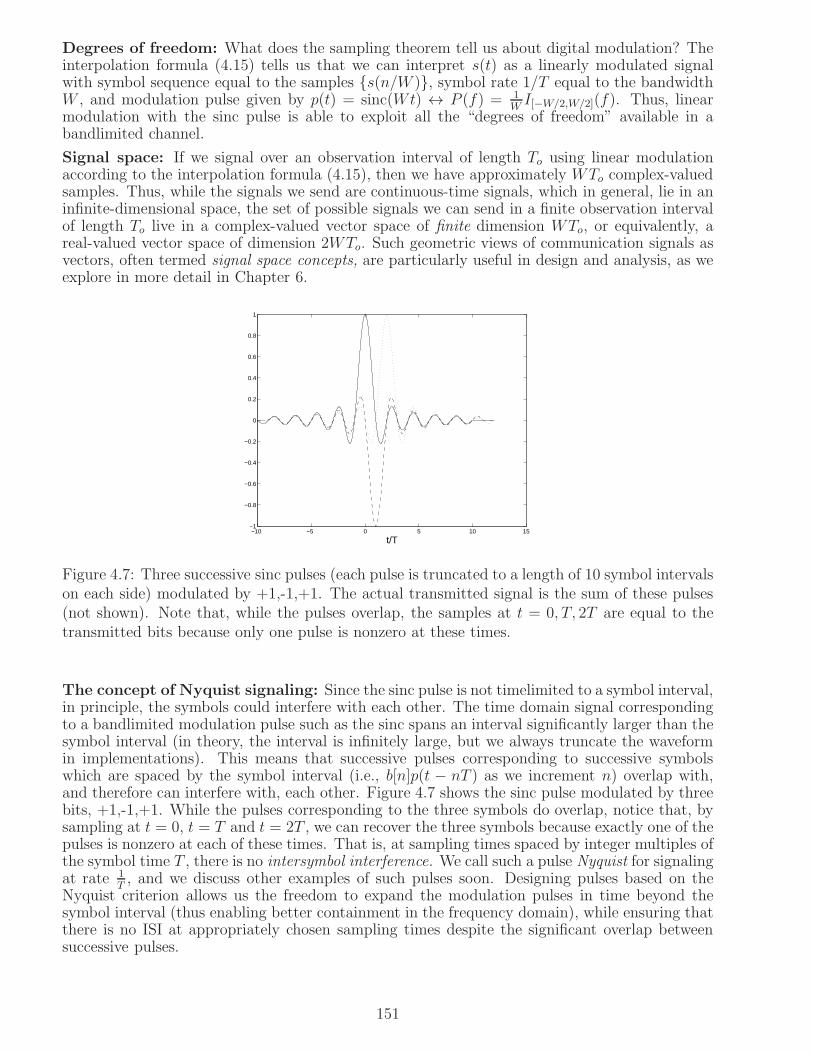
Degrees of freedom: What does the sampling theorem tell us about digital modulation? Theinterpolation formula (4.15) tells us that we can interpret s(t) as a linearly modulated signalwith symbol sequence equal to the samples s(n/W ), symbol rate 1/T equal to the bandwidthW , and modulation pulse given by p(t) = sinc(Wt) ↔ P (f) = 1

WI[−W/2,W/2](f). Thus, linear

modulation with the sinc pulse is able to exploit all the “degrees of freedom” available in abandlimited channel.

Signal space: If we signal over an observation interval of length To using linear modulationaccording to the interpolation formula (4.15), then we have approximately WTo complex-valuedsamples. Thus, while the signals we send are continuous-time signals, which in general, lie in aninfinite-dimensional space, the set of possible signals we can send in a finite observation intervalof length To live in a complex-valued vector space of finite dimension WTo, or equivalently, areal-valued vector space of dimension 2WTo. Such geometric views of communication signals asvectors, often termed signal space concepts, are particularly useful in design and analysis, as weexplore in more detail in Chapter 6.

−10 −5 0 5 10 15−1

−0.8

−0.6

−0.4

−0.2

0

0.2

0.4

0.6

0.8

1

t/T

Figure 4.7: Three successive sinc pulses (each pulse is truncated to a length of 10 symbol intervalson each side) modulated by +1,-1,+1. The actual transmitted signal is the sum of these pulses(not shown). Note that, while the pulses overlap, the samples at t = 0, T, 2T are equal to thetransmitted bits because only one pulse is nonzero at these times.

The concept of Nyquist signaling: Since the sinc pulse is not timelimited to a symbol interval,in principle, the symbols could interfere with each other. The time domain signal correspondingto a bandlimited modulation pulse such as the sinc spans an interval significantly larger than thesymbol interval (in theory, the interval is infinitely large, but we always truncate the waveformin implementations). This means that successive pulses corresponding to successive symbolswhich are spaced by the symbol interval (i.e., b[n]p(t − nT ) as we increment n) overlap with,and therefore can interfere with, each other. Figure 4.7 shows the sinc pulse modulated by threebits, +1,-1,+1. While the pulses corresponding to the three symbols do overlap, notice that, bysampling at t = 0, t = T and t = 2T , we can recover the three symbols because exactly one of thepulses is nonzero at each of these times. That is, at sampling times spaced by integer multiples ofthe symbol time T , there is no intersymbol interference. We call such a pulse Nyquist for signalingat rate 1

T, and we discuss other examples of such pulses soon. Designing pulses based on the

Nyquist criterion allows us the freedom to expand the modulation pulses in time beyond thesymbol interval (thus enabling better containment in the frequency domain), while ensuring thatthere is no ISI at appropriately chosen sampling times despite the significant overlap betweensuccessive pulses.

151

−10 −5 0 5 10 15 20−1.5

−1

−0.5

0

0.5

1

1.5

t/T

Figure 4.8: The baseband signal for 10 BPSK symbols of alternating signs, modulated using thesinc pulse. The first symbol is +1, and the sample at time t = 0, marked with ’x’, equals +1, asdesired (no ISI). However, if the sampling time is off by 0.25T , the sample value, marked by ’+’,becomes much smaller because of ISI. While it still has the right sign, the ISI causes it to havesignificantly smaller noise immunity. See Problem 4.14 for an example in which the ISI due totiming mismatch actually causes the sign to flip.

152

The problem with sinc: Are we done then? Should we just use linear modulation with a sincpulse when confronted with a bandlimited channel? Unfortunately, the answer is no: just as therectangular timelimited pulse decays too slowly in frequency, the rectangular bandlimited pulse,corresponding to the sinc pulse in the time domain, decays too slowly in time. Let us see whathappens as a consequence. Figure 4.8 shows a plot of the modulated waveform for a bit sequenceof alternating sign. At the correct sampling times, there is no ISI. However, if we consider a smalltiming error of 0.25T , the ISI causes the sample value to drop drastically, making the systemmore vulnerable to noise. What is happening is that, when there is a small sampling offset,we can make the ISI add up to a large value by choosing the interfering symbols so that theircontributions all have signs opposite to that of the desired symbol at the sampling time. Sincethe sinc pulse decays as 1/t, the ISI created for a given symbol by an interfering symbol whichis n symbol intervals away decays as 1/n, so that, in the worst-case, the contributions from theinterfering symbols roughly have the form

∑

n1n, a series that is known to diverge. Thus, in

theory, if we do not truncate the sinc pulse, we can make the ISI arbitrarily large when there isa small timing offset. In practice, we do truncate the modulation pulse, so that we only see ISIfrom a finite number of symbols. However, even when we do truncate, as we see from Figure 4.8,the slow decay of the sinc pulse means that the ISI adds up quickly, and significantly reducesthe margin of error when noise is introduced into the system.

While the sinc pulse may not be a good idea in practice, the idea of using bandwidth-efficientNyquist pulses is a good one, and we now develop it further.

4.3.2 Nyquist Criterion for ISI Avoidance

Nyquist signaling: Consider a linearly modulated signal

u(t) =∑

n

b[n]p(t− nT )

We say that the pulse p(t) is Nyquist (or satisfies the Nyquist criterion) for signaling at rate 1T

if the symbol-spaced samples of the modulated signal are equal to the symbols (or a fixed scalarmultiple of the symbols); that is, u(kT ) = b[k] for all k. That is, there is no ISI at appropriatelychosen sampling times spaced by the symbol interval.

In the time domain, it is quite easy to see what is required to satisfy the Nyquist criterion. Thesamples u(kT ) =

∑

n b[n]p(kT − nT ) = b[k] (or a scalar multiple of b[k]) for all k if and onlyif p(0) = 1 (or some nonzero constant) and p(mT ) = 0 for all integers m 6= 0. However, fordesign of bandwidth efficient pulses, it is important to characterize the Nyquist criterion in thefrequency domain. This is given by the following theorem.

Theorem 4.3.2 (Nyquist criterion for ISI avoidance): The pulse p(t) ↔ P (f) is Nyquistfor signaling at rate 1

Tif

p(mT ) = δm0 =

1 m = 00 m 6= 0

(4.16)

or equivalently,1

T

∞∑

k=−∞P (f +

k

T) = 1 for all f (4.17)

The proof of this theorem is given in Section 4.5, where we show that both the Nyquist samplingtheorem, Theorem 4.3.1, and the preceding theorem are based on the same mathematical result,that the samples of a time domain signal have a one-to-one mapping with the sum of translated(or aliased) versions of its Fourier transform.

153

In this section, we explore the design implications of Theorem 4.3.2. In the frequency domain,the translates of P (f) by integer multiples of 1/T must add up to a constant. As illustrated byFigure 4.9, the minimum bandwidth pulse for which this happens is the ideal bandlimited pulseover an interval of length 1/T .

Not Nyquist

P(f)P(f + 1/T) P(f − 1/T)

1/T

f

... ...... ...P(f)P(f + 1/T) P(f − 1/T)

1/T

f

Nyquist with minimum bandwidth

Figure 4.9: The minimum bandwidth Nyquist pulse is a sinc.

Minimum bandwidth Nyquist pulse: The minimum bandwidth Nyquist pulse is

P (f) =

T, |f | ≤ 12T

0, else

corresponding to the time domain pulse

p(t) = sinc(t/T )

As we have already discussed, the sinc pulse is not a good choice in practice because of its slowdecay in time. To speed up the decay in time, we must expand in the frequency domain, whileconforming to the Nyquist criterion. The trapezoidal pulse depicted in Figure 4.9 is an exampleof such a pulse.

P(f + 1/T)

(1+a)/(2T)(1−a)/(2T)−(1−a)/(2T)−(1+a)/(2T)f

T P(f) P(f − 1/T)

Figure 4.10: A trapezoidal pulse which is Nyquist at rate 1/T . The (fractional) excess bandwidthis a.

The role of excess bandwidth: We have noted earlier that the problem with the sinc pulsearises because of its 1/t decay and the divergence of the harmonic series

∑∞n=1

1n, which implies

that the worst-case contribution from “distant” interfering symbols at a given sampling instantcan blow up. Using the same reasoning, however, a pulse p(t) decaying as 1/tb for b > 1 shouldwork, since the series

∑∞n=1

1nb does converge for b > 1. A faster time decay requires a slower

decay in frequency. Thus, we need excess bandwidth, beyond the minimum bandwidth dictatedby the Nyquist criterion, to fix the problems associated with the sinc pulse. The (fractional)excess bandwidth for a linear modulation scheme is defined to be the fraction of bandwidthover the minimum required for ISI avoidance at a given symbol rate. In particular, Figure 4.10shows that a trapezoidal pulse (in the frequency domain) can be Nyquist for suitably chosenparameters, since the translates P (f+k/T ) as shown in the figure add up to a constant. Sincetrapezoidal P (f) is the convolution of two boxes in the frequency domain, the time domain pulsep(t) is the product of two sinc functions, as worked out in the example below. Since each sincdecays as 1/t, the product decays as 1/t2, which implies that the worst-case ISI with timingmismatch is indeed bounded.

154

Example 4.3.1 Consider the trapezoidal pulse of excess bandwidth a shown in Figure 4.10.(a) Find an explicit expression for the time domain pulse p(t).(b) What is the bandwidth required for a passband system using this pulse operating at 120Mbps using 64QAM, with an excess bandwidth of 25%?Solution: (a) It is easy to check that the trapezoid is a convolution of two boxes as follows (weassume 0 < a ≤ 1):

P (f) =T 2

aI[− 1

2T, 12T

](f) ∗ I[− a2T

, a2T

](f)

Taking inverse Fourier transforms, we obtain

p(t) =T 2

a

(

1

Tsinc(t/T )

)

( a

Tsinc(at/T )

)

= sinc(t/T )sinc(at/T ) (4.18)

The presence of the first sinc provides the zeroes required by the time domain Nyquist criterion:p(mT ) = 0 for nonzero integers m 6= 0. The presence of a second sinc yields a 1/t2 decay,providing robustness against timing mismatch.(b) Since 64 = 26, the use of 64QAM corresponding to sending 6 bits/symbol, so that the symbolrate is 120/6 = 20 Msymbols/sec. The minimum bandwidth required is therefore 20 MHz, sothat 25% excess bandwidth corresponds to a bandwidth of 20× 1.25 = 25 MHz.

Raised cosine pulse: Replacing the straight line of the trapezoid with a smoother cosine-shaped curve in the frequency domain gives us the raised cosine pulse shown in Figure 4.12,which has a faster, 1/t3, decay in the time domain.

P (f) =

T, |f | ≤ 1−a2T

T2[1 + cos((|f | − 1−a

2T)πT

a)], 1−a

2T≤ |f | ≤ 1+a

2T

0, |f | > 1+a2T

where a is the fractional excess bandwidth, typically chosen in the range where 0 ≤ a < 1. Asshown in Problem 4.11, the time domain pulse s(t) is given by

p(t) = sinc(t

T)cos πa t

T

1−(

2atT

)2

This pulse inherits the Nyquist property of the sinc pulse, while having an additional multiplica-tive factor that gives an overall 1/t3 decay with time. The faster time decay compared to thesinc pulse is evident from a comparison of Figures 4.12(b) and 4.11(b).

4.3.3 Bandwidth efficiency

We define the bandwidth efficiency of linear modulation with an M-ary alphabet as

ηB = log2M bits/symbol

The Nyquist criterion for ISI avoidance says that the minimum bandwidth required for ISI-freetransmission using linear modulation equals the symbol rate, using the sinc as the modulationpulse. For such an idealized system, we can think of ηB as bits/second per Hertz, since the symbolrate equals the bandwidth. Thus, knowing the bit rate Rb and the bandwidth efficiency ηB ofthe modulation scheme, we can determine the symbol rate, and hence the minimum requiredbandwidth Bmin. as follows:

Bmin =Rb

ηB

155

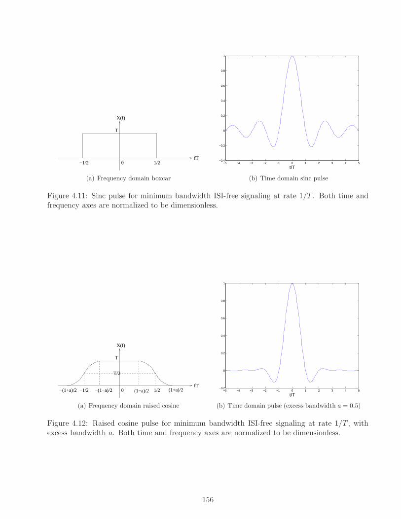
−1/2 1/2fT

T

0

X(f)

(a) Frequency domain boxcar

−5 −4 −3 −2 −1 0 1 2 3 4 5−0.4

−0.2

0

0.2

0.4

0.6

0.8

1

t/T

(b) Time domain sinc pulse

Figure 4.11: Sinc pulse for minimum bandwidth ISI-free signaling at rate 1/T . Both time andfrequency axes are normalized to be dimensionless.

−(1−a)/2 (1+a)/2(1−a)/2 1/2fT

T

T/2

0

X(f)

−(1+a)/2 −1/2

(a) Frequency domain raised cosine

−5 −4 −3 −2 −1 0 1 2 3 4 5−0.2

0

0.2

0.4

0.6

0.8

1

t/T

(b) Time domain pulse (excess bandwidth a = 0.5)

Figure 4.12: Raised cosine pulse for minimum bandwidth ISI-free signaling at rate 1/T , withexcess bandwidth a. Both time and frequency axes are normalized to be dimensionless.

156

This bandwidth would then be expanded by the excess bandwidth used in the modulating pulse.However, this is not included in our definition of bandwidth efficiency, because excess bandwidthis a highly variable quantity dictated by a variety of implementation considerations. Once wedecide on the fractional excess bandwidth a, the actual bandwidth required is

B = (1 + a)Bmin = (1 + a)Rb

ηB

4.3.4 Power-bandwidth tradeoffs: a sneak preview

Clearly, we can increase bandwidth efficiency simply by increasing M , the constellation size.For example, the bandwidth efficiency of QPSK is 2 bits/symbol, while that of 16QAM is 4bits/symbol. What stops us from increasing constellation size, and hence bandwidth efficiency,indefinitely is noise, and the fact that we cannot use arbitrarily large transmit power (typicallylimited by cost or physical and regulatory constraints) to overcome it. Noise in digital communi-cation systems must be modeled statistically, hence rigorous discussion of a formal model and itsdesign consequences is postponed to Chapters 5 and 6. However, that does not prevent us fromgiving a handwaving sneak preview of the bottomline here. Note that this subsection is meantas a teaser: it can be safely skipped, since these issues are covered in detail in Chapter 6.

−1

min

dmin

EsEs

of two

by factorScale up

−1 1

1

2

−2

−2 2

d

Figure 4.13: Scaling of minimum distance and energy per symbol.

Intuitively speaking, the effect of noise is to perturb constellation points from the nominal loca-tions shown in Figure 4.4, which leads to the possibility of making an error in deciding whichpoint was transmitted. For a given noise “strength” (which determines how much movement thenoise can produce), the closer the constellation points, the more the possibility of such errors.In particular, as we shall see in Chapter 6, the minimum distance between constellation points,termed dmin, provide a good measure of how vulnerable we are to noise. For a given constellationshape, we can increase dmin simply by scaling up the constellation, as shown in Figure 4.13, butthis comes with a corresponding increase in energy expenditure. To quantify this, define theenergy per symbol Es for a constellation as the average of the squared Euclidean distances of thepoints from the origin. For an M-ary constellation, each symbol carries log2M bits of informa-tion, and we can define the average energy per bit Eb as Eb =

Es

log2 M. Specifically, dmin increases

from 2 to 4 by scaling as shown in Figure 4.13. Correspondingly, Es = 2 and Eb = 1 is increasedto Es = 8 and Eb = 4 in Figure 4.13(b). Thus, doubling the minimum distance in Figure 4.13

leads to a four-fold increase in Es and Eb. However, the quantityd2min

Ebdoes not change due to

scaling; it depends only on the relative geometry of the constellation points. We therefore adopt

157

this scale-invariant measure as our notion of power efficiency for a constellation:

ηP =d2min

Eb(4.19)

Since this quantity is scale-invariant, we can choose any convenient scaling in computing it: forQPSK, choosing the scaling on the left in Figure 4.13, we have dmin = 2, Es = 2, Eb = 1, whichgives ηP = 4.

It is important to understand how these quantities relate to physical link parameters. For agiven bit rate Rb and received power PRX , the energy per bit is given by Eb =

PRX

Rb. It is worth

verifying that the units make sense: the numerator has units of Watts, or Joules/sec, while thedenominator has units of bits/sec, so that Eb has units of joules/bit. We shall see in Chapter 6that the reliability of communication is determined by the power efficiency ηP (a scale-invariantquantity which is a function of the constellation shape) and the dimensionless signal-to-noise ratio(SNR) measure Eb/N0, where N0 is the noise power spectral density, which has units of watts/Hz,or Joules. Specifically, the reliability can be approximately characterized by the product ηP

Eb

N0, so

that, for a given desired reliability, the required energy per bit (and hence power) scales inverselyas power efficiency for a fixed bit rate. Communication link designers use such concepts as thebasis for forming a “link budget” that can be used to choose link parameters such as transmitpower, antenna gains and range.

Even based on these rather sketchy and oversimplified arguments, we can draw quick conclusionson the power-bandwidth tradeoffs in using different constellations, as shown in the followingexample.

Example 4.3.2 We wish to design a passband communication system operating at a bit rate of40 Mbps.(a) What is the bandwidth required if we employ QPSK, with an excess bandwidth of 25%.(b) What if we now employ 16QAM, again with excess bandwidth 25%.(c) Suppose that the QPSK system in (a) attains a desired reliability when the transmit power is50 mW. Give an estimate of the transmit power needed for the 16QAM system in (b) to attaina similar reliability.(d) How does the bandwidth and transmit power required change for the QPSK system if weincrease the bit rate to 80 Mbps.(e) How does the bandwidth and transmit power required change for the QPSK system if weincrease the bit rate to 80 Mbps.Solution: (a) The bandwidth efficiency of QPSK is 2 bits/symbol, hence the minimum bandwidthrequired is 20 MHz. For excess bandwidth of 25%, the bandwidth required is 25 MHz.(b) The bandwidth efficiency of 16QAM is 4 bits/symbol, hence, reasoning as in (a), the band-width required is 12.5 MHz.(c) We wish to set ηPEb/N0 to be equal for both systems in order to keep the reliability roughlythe same. Assuming that the noise PSD N0 is the same for both systems, the required Eb scalesas 1/ηP . Since the bit rates Rb for both systems are equal, the required received power P = EbRb

(and hence the required transmit power, assuming that received power scales linearly with trans-mit power) also scales as 1/ηP . We already know that ηP = 4 for QPSK. It remains to find ηP for16QAM, which is shown in Problem 4.15 to equal 8/5. We therefore conclude that the transmitpower for the 16QAM system can be estimated as

PT (16QAM) = PT (QPSK)ηP (QPSK)

ηP (16QAM)

which evaluates for 125 mW.(d) For fixed bandwidth efficiency, required bandwidth scales linearly with bit rate, hence the

158

new bandwidth required is 50 MHz. In order to maintain a given reliability, we must maintainthe same value of ηPEb/N0 as in (c). The power efficiency ηP is unchanged, since we are usingthe same constellation. Assuming that the noise PSD N0 is unchanged, the required energy perbit Eb is unchanged, hence transmit power must scale up linearly with bit rate Rb. Thus, thepower required using QPSK is now 100 mW.(e) Arguing as in (d), we require a bandwidth of 25 MHz and a power of 250 mW for 16QAM,using the results in (b) and (c).

4.3.5 The Nyquist criterion at the link level

z(t)

TX g (t)C

g (t)RX

Transmit Filter Channel Filter Receive FilterSymbols

rate 1/T

b[n]Sampler

rate 1/T

z(nT)

When is z(nT) = b[n]? g (t)

Figure 4.14: Nyquist criterion at the link level.

Figure 4.14 shows a block diagram for a link using linear modulation, with the entire modelexpressed in complex baseband. The symbols b[n] are passed through the transmit filter toobtain the waveform

∑

n b[n]gTX(t − nT ). This then goes through the channel filter gC(t), andthen the receive filter gRX(t). Thus, at the output of the receive filter, we have the linearlymodulated signal

∑

n b[n]p(t − nT ), where p(t) = (gTX ∗ gC ∗ gRX)(t) is the cascade of thetransmit, channel and receive filters. We would like the pulse p(t) to be Nyquist at rate 1/T , sothat, in the absence of noise, the symbol rate samples at the output of the receive filter equalthe transmitted symbols. Of course, in practice, we do not have control over the channel, hencewe often assume an ideal channel, and design such that the cascade of the transmit and receivefilter, given by (gTX ∗ gRX) (t)GTX(f)GRX(f) is Nyquist. One possible choice is to set GTX tobe a Nyquist pulse, and GRX to be a wideband filter whose response is flat over the band ofinterest. Another choice that is even more popular is to set GTX(f) and GRX(f) to be squareroots of a Nyquist pulse. In particular, the square root raised cosine (SRRC) pulse is often usedin practice.

A framework for software simulations of linear modulated systems with raised cosine and SRRCpulses, including Matlab code fragments, is provided in the appendix, and provides a foundationfor Software Lab 4.1.

Square root Nyquist pulses and their time domain interpretation: A pulse g(t) ↔ G(f)is defined to be square root Nyquist at rate 1/T if |G(f)|2 is Nyquist at rate 1/T . Note thatP (f) = |G(f)|2 ↔ p(t) = (g ∗ gMF )(t), where gMF (t) = g∗(−t). The time domain Nyquistcondition is given by

p(mT ) = (g ∗ gMF )(mT ) =

∫

g(t)g∗(t−mT )dt = δm0 (4.20)

That is, a square root Nyquist pulse has an autocorrelation function that vanishes at nonzerointeger multiples of T . In other words, the waveforms g(t− kT, k = 0,±1,±2, ... are orthonor-mal, and can be used to provide a basis for constructing more complex waveforms, as we see inSection 4.3.6.

Food for thought: True or False? Any pulse timelimited to [0, T ] is square root Nyquist atrate 1/T .

159

4.3.6 Linear modulation as a building block

Linear modulation can be used as a building block for constructing more sophisticated waveforms,using discrete-time sequences modulated by square root Nyquist pulses. Thus, one symbol wouldbe made up of multiple “chips,” linearly modulated by a square root Nyquist “chip waveform.”Specifically, suppose that ψ(t) is square root Nyquist at a chip rate 1

Tc. N chips make up

one symbol, so that the symbol rate is 1Ts

= 1NTc

, and a symbol waveform is given by linearly

modulating a code vector s = (s[0], ..., s[N − 1]) consisting of N chips, as follows:

s(t) =N∑

k=0

s[k]ψ(t− kTc)

Since ψ(t− kTc) are orthonormal (see (4.20)), we have simply expressed the code vector in acontinuous time basis. Thus, the continuous time inner product between two symbol waveforms(which determines their geometric relationships and their performance in noise, as we see inthe next chapter) is equal to the discrete time inner product between the corresponding codevectors. Specifically, suppose that s1(t) and s2(t) are two symbol waveforms corresponding tocode vectors s1 and s2, respectively. Then their inner product satisfies

〈s1, s2〉 =N−1∑

k=0

N−1∑

l=0

s1[k]s∗2[l]

∫

ψ(t− kTc)ψ∗(t− lTc)dt =

N−1∑

k=0

s1[k]s∗2[k] = 〈s1, s2〉

where we have use the orthonormality of the translates ψ(t − kTc). This means that we candesign discrete time code vectors to have certain desired properties, and then linearly modulatesquare root Nyquist chip waveforms to get symbol waveforms that have the same desired prop-erties. For example, if s1 and s2 are orthogonal, then so are s1(t) and s2(t); we use this in thenext section when we discuss orthogonal modulation.

Examples of square root Nyquist chip waveforms include a rectangular pulse timelimited to aninterval of length Tc , as well as bandlimited pulses such as the square root raised cosine. FromTheorem 4.2.1, we see that the PSD of the modulated waveform is proportional to |Ψ(f)|2 (it istypically a good approximation to assume that the chips s[k] are uncorrelated). That is, thebandwidth occupancy is determined by that of the chip waveform ψ.

4.4 Orthogonal and Biorthogonal Modulation

While linear modulation with larger and larger constellations is a means of increasing bandwidthefficiency, we shall see that orthogonal modulation with larger and larger constellations is ameans of increasing power efficiency (at the cost of making the bandwidth efficiency smaller).Consider first M-ary frequency shift keying (FSK), a classical form of orthogonal modulation inwhich one of M sinusoidal tones, successively spaced by ∆f , are transmitted every T units oftime, where 1

Tis the symbol rate. Thus, the bit rate is log2 M

T, and for a typical symbol interval,

the transmitted passband signal is chosen from one of M possibilities:

up,k(t) = cos (2π(f0 + k∆f)t) , 0 ≤ t ≤ T, k = 0, 1, ...,M − 1

where we typically have f0 ≫ 1T. Taking f0 as reference, the corresponding complex baseband

waveforms areuk(t) = exp (j2πk∆ft) , 0 ≤ t ≤ T, k = 0, 1, ...,M − 1

160

Let us now understand how the tones should be chosen in order to ensure orthogonality. Recallthat the passband and complex baseband inner products are related as follows:

〈up,k, up,l〉 =1

2Re〈uk, ul〉

so we can develop criteria for orthogonality working in complex baseband. Setting k = l, we seethat

||uk||2 = T

For two adjacent tones, l = k + 1, we leave it as an exercise to show that

Re〈uk, uk+1〉 =sin 2π∆fT

2π∆f

We see that the minimum value of ∆f for which the preceding quantity is zero is given by2π∆fT = π, or ∆f = 1

2T.

Thus, from the point of view of the receiver, a tone spacing of 12T

ensures that when there is anincoming wave at the kth tone, then correlating against the kth tone will give a large output, butcorrelating against the (k + 1)th tone will give zero output (in the absence of noise). However,this assumes a coherent system in which the tones we are correlating against are synchronized inphase with the incoming wave. What happens if they are 90 out of phase? Then correlation ofthe kth tone with itself yields

∫ T

0

cos (2π(f0 + k∆f)t) cos(

2π(f0 + k∆f)t+π

2

)

dt = 0

(by orthogonality of the cosine and sine), so that the output we desire to be large is actuallyzero! Robustness to such variations can be obtained by employing noncoherent reception, whichwe describe next.

Noncoherent reception: Let us develop the concept of noncoherent reception in generality,because it is a concept that is useful in many settings, not just for orthogonal modulation. Sup-pose that we transmit a passband waveform, and wish to detect it at the receiver by correlatingit against the receiver’s copy of the waveform. However, the receiver’s local oscillator may notbe synchronized in phase with the phase of the incoming wave. Let us denote the receiver’s copyof the signal as

up(t) = uc(t) cos 2πfct− us(t) sin 2πfct

and the incoming passband signal as

yp(t) = yc(t) cos 2πfct− ys(t) sin 2πfct = uc(t) cos (2πfct+ θ)− us(t) sin (2πfct+ θ)

Using the receiver’s local oscillator as reference, the complex envelope of the receiver’s copy isu(t) = uc + jus(t), while that of the incoming wave is y(t) = u(t)ejθ. Thus, the inner product

〈yp, up〉 =1

2Re〈y, u〉 = 1

2Re〈uejθ, u〉 = 1

2Re(

||u||2ejθ)

=||u||22

cos θ

Thus, the output of the correlator is degraded by the factor cos θ, and can actually become zero,as we have already observed, if the phase offset θ = π/2. In order to get around this problem,let us look at the complex baseband inner product again:

〈y, u〉 = 〈uejθ, u〉 = ejθ||u||2

161

We could ensure that this output remains large regardless of the value of θ if we took its magni-tude, rather than the real part. Thus, noncoherent reception corresponds to computing |〈y, u〉|or |〈y, u〉|2. Let us unwrap the complex inner product to see what this entails:

〈y, u〉 =∫

y(t)u∗(t)dt =

∫

(yc(t)+jys(t))(uc(t)−jus(t))dt = (〈yc, uc〉+ 〈ys, us〉)+j (〈ys, uc〉 − 〈yc, us〉)

Thus, the noncoherent receiver computes the quantity

|〈y, u〉|2 = (〈yc, uc〉+ 〈ys, us〉)2 + (〈ys, uc〉 − 〈yc, us〉)2

In contrast, the coherent receiver computes

Re〈y, u〉 = 〈yc, uc〉+ 〈ys, us〉

That is, when the receiver LO is synchronized to the phase of the incoming wave, we can correlatethe I component of the received waveform with the I component of the receiver’s copy, andsimilarly correlate the Q components, and sum them up. However, in the presence of phaseasynchrony, the I and Q components get mixed up, and we must compute the magnitude of thecomplex inner product to recover all the energy of the incoming wave. Figure 4.15 shows thereceiver operations corresponding to coherent and noncoherent reception.

Squarer

Squarer receiveroutput

)Coherent receiver output

PassbandReceivedSignal

c

c

s

su (t)

u (t)

u (t)

u (t)

Z s

cZ

Low PassFilter

cπ− 2 sin 2 f t

2 cos 2 f tcπ

Low PassFilter

y (t)c

y (t)s

− Noncoherent

Figure 4.15: Structure of coherent and noncoherent receivers.

Back to FSK: Going back to FSK, if we now use noncoherent reception, then in order toensure that we get a zero output (in the absence of noise) when receiving the kth tone with anoncoherent receiver for the (k + 1)th tone, we must ensure that

|〈uk, uk+1〉| = 0

We leave it as an exercise (Problem 4.18) to show that the minimum tone spacing for noncoherentFSK is 1

T, which is double that required for orthogonality in coherent FSK. The bandwidth for

coherent M-ary FSK is approximately M2T, which corresponds to a time-bandwidth product of

approximately M2. This corresponds to a complex vector space of dimension M

2, or a real vector

space of dimension M , in which we can fit M orthogonal signals. On the other hand, M-arynoncoherent signaling requires M complex dimensions, since the complex baseband signals mustremain orthogonal even under multiplication by complex-valued scalars.

Summarizing the concept of orthogonality: To summarize, when we say “orthogonal”modulation, we must specify whether we mean coherent or noncoherent reception, because the

162

concept of orthogonality is different in the two cases. For a signal set sk(t), orthogonalityrequires that, for k 6= l, we have

Re(〈sk, sl〉) = 0 coherent orthogonality criterion〈sk, sl〉 = 0 noncoherent orthogonality criterion

(4.21)

Bandwidth efficiency: We conclude from the example of orthogonal FSK that the bandwidth

efficiency of orthogonal signaling is ηB = log2(2M)M

bits/complex dimension for coherent systems,

and ηB = log2(M)M

bits/complex dimension for noncoherent systems. This is a general observationthat holds for any realization of orthogonal signaling. In a signal space of complex dimensionD (and hence real dimension 2D), we can fit 2D signals satisfying the coherent orthogonalitycriterion, but only D signals satisfying the noncoherent orthogonality criterion. AsM gets large,the bandwidth efficiency tends to zero. In compensation, as we see in Chapter 6, the powerefficiency of orthogonal signaling for large M is the “best possible.”

Orthogonal Walsh-Hadamard codes

Section 4.3.6 shows how to map vectors to waveforms while preserving inner products, by usinglinear modulation with a square root Nyquist chip waveform. Applying this construction, theproblem of designing orthogonal waveforms si now reduces to designing orthogonal code vectorssi. Walsh-Hadamard codes are a standard construction employed for this purpose, and canbe constructed recursively as follows: at the nth stage, we generate 2n orthogonal vectors, usingthe 2n−1 vectors constructed in the n − 1 stage. Let Hn denote a matrix whose rows are 2n

orthogonal codes obtained after the nth stage, with H0 = (1). Then

Hn =

(

Hn−1 Hn−1

Hn−1 −Hn−1

)

We therefore get

H1 =

(

1 11 −1

)

, H2 =

1 1 1 11 −1 1 −11 1 −1 −11 −1 −1 1

, etc.

Figure 4.16 depicts the waveforms corresponding to the 4-ary signal set in H2 using a rectangulartimelimited chip waveform to go from sequences to signals, as described in Section 4.3.6.

The signals si obtained above can be used for noncoherent orthogonal signaling, since theysatisfy the orthogonality criterion 〈si, sj〉 = 0 for i 6= j. However, just as for FSK, we canfit twice as many signals into the same number of degrees of freedom if we used the weakernotion of orthogonality required for coherent signaling, namely Re(〈si, sj〉 = 0 for i 6= j. Itis easy to check that for M-ary Walsh-Hadamard signals si, i = 1, ...,M, we can get 2Morthogonal signals for coherent signaling: si, jsi, i = 1, ...,M. This construction correspondsto independently modulating the I and Q components with a Walsh-Hadamard code; that is,using passband waveforms si(t) cos 2πfct and−si(t) sin 2πfct (the negative sign is only to conformto our convention for I and Q, and can be dropped, which corresponds to replacing jsi by −jsiin complex baseband), i = 1, ...,M .

Biorthogonal modulation

Given an orthogonal signal set, a biorthogonal signal set of twice the size can be obtained byincluding a negated copy of each signal. Since signals s and −s cannot be distinguished in anoncoherent system, biorthogonal signaling is applicable to coherent systems. Thus, for anM-aryWalsh-Hadamard signal set si withM signals obeying the noncoherent orthogonality criterion,we can construct a coherent orthogonal signal set si, jsi of size 2M , and hence a biorthogonalsignal set of size 4M , e.g., si, jsi,−si,−jsi. These correspond to the 4M passband waveforms±si(t) cos 2πfct and ±si(t) sin 2πfct, i = 1, ...,M .

163

Figure 4.16: Walsh-Hadamard codes for 4-ary orthogonal modulation.

4.5 Proofs of the Nyquist theorems

We have used Nyquist’s sampling theorem, Theorem 4.3.1, to argue that linear modulationusing the sinc pulse is able to use all the degrees of freedom in a bandlimited channel. Onthe other hand, Nyquist’s criterion for ISI avoidance, Theorem 4.3.2, tells us, roughly speaking,that we must have enough degrees of freedom in order to avoid ISI (and that the sinc pulseprovides the minimum such degrees of freedom). As it turns out, both theorems are based onthe same mathematical relationship between samples in the time domain and aliased spectra inthe frequency domain, stated in the following theorem.

Theorem 4.5.1 (Sampling and Aliasing): Consider a signal s(t), sampled at rate 1Ts. Let

S(f) denote the spectrum of s(t), and let

B(f) =1

Ts

∞∑

k=−∞S(f +

k

Ts) (4.22)

denote the sum of translates of the spectrum. Then the following observations hold:(a) B(f) is periodic with period 1

Ts.

(b) The samples s(nTs) are the Fourier series for B(f), satisfying

s(nTs) = Ts

∫ 12Ts

− 12Ts

B(f)ej2πfnTs df (4.23)

B(f) =∞∑

n=−∞s(nTs)e

−j2πfnTs (4.24)

Remark: Note that the signs of the exponents for the frequency domain Fourier series in thetheorem are reversed from the convention in the usual time domain Fourier series (analogous tothe reversal of the sign of the exponent for the inverse Fourier transform compared to the Fouriertransform).

164

Proof of Theorem 4.5.1: The periodicity of B(f) follows by its very construction. To prove(b), apply the the inverse Fourier transform to obtain

s(nTs) =

∫ ∞

−∞S(f)ej2πfnTsdf

We now write the integral as an infinite sum of integrals over segments of length 1/T

s(nTs) =∞∑

k=−∞

∫

k+12

Ts

k− 12

Ts

S(f)ej2πfnTsdf

In the integral over the kth segment, make the substitution ν = f − kTs

and rewrite it as

∫ 12Ts

− 12Ts

S(ν +k

Ts)ej2π(ν+

kTs

)nTsdν =

∫ 12Ts

− 12Ts

S(ν +k

Ts)ej2πνnTsdν

Now that the limits of all segments and the complex exponential in the integrand are the same(i.e., independent of k), we can move the summation inside to obtain

s(nTs) =∫

12Ts

− 12Ts

(

∑∞k=−∞ S(ν + k

Ts))

ej2πνnTsdν

= Ts∫

12Ts

− 12Ts

B(ν)ej2πνnTsdν

proving (4.23). We can now recognize that this is just the formula for the Fourier series coefficientsof B(f), from which (4.24) follows.

to recover S(f) from B(f)

s 1/Ts1/TsS(f + ) 1/TsS(f − ) 1/TsS(f + ) 1/TsS(f − )

W W

f f

S(f) S(f)

Sampling rate not high enough Sampling rate high enoughto recover S(f) from B(f)

1/T

Figure 4.17: Recovering a signal from its samples requires a high enough sampling rate fortranslates of the spectrum not to overlap.

Inferring Nyquist’s sampling theorem from Theorem 4.5.1: Suppose that s(t) is ban-dlimited to [−W

2, W

2]. The samples of s(t) at rate 1

Tscan be used to reconstruct B(f), since they

are the Fourier series for B(f). But S(f) can be recovered from B(f) if and only if the translatesS(f − k

Ts) do not overlap, as shown in Figure 4.17. This happens if and only if 1

Ts≥ W . Once

this condition is satisfied, 1TsS(f) can be recovered from B(f) by passing it through an ideal

bandlimited filter H(f) = I[−W/2.W/2](f). We therefore obtain that

1

TsS(f) = B(f)H(f) =

∞∑

n=−∞s(nTs)e

−j2πfnTsI[−W/2.W/2](f) (4.25)

Noting that I[−W/2.W/2](f) ↔W sinc(Wt), we have

e−j2πfnTsI[−W/2.W/2](f) ↔W sinc (W (t− nTs))

165

Taking inverse Fourier transforms, we get the interpolation formula

1

Tss(t) =

∞∑

n=−∞s(nTs)W sinc (W (t− nTs))

which reduces to (4.15) for 1Ts

= W . This completes the proof of the sampling theorem, Theorem4.3.1.

Inferring Nyquist’s criterion for ISI avoidance from Theorem 4.5.1: A Nyquist pulsep(t) at rate 1/T must satisfy p(nT ) = δn0. Applying Theorem 4.5.1 with s(t) = p(t) and Ts = T ,it follows immediately from (4.24) that p(nT ) = δn0 (i.e., the time domain Nyquist criterionholds) if and only if

B(f) =1

T

∞∑

k=−∞P (f +

k

Ts) = 1

In other words, if the Fourier series only has a DC term, then the periodic waveform it correspondsto must be constant.


This chapter provides an introduction to how bits can be translated to information-carryingsignals which satisfy certain constraints (e.g., fitting within a given frequency band). We focuson linear modulation over passband channels.

Modulation basics• Information bits can be encoded into two-dimensional (complex-valued) constellations, whichcan be modulated onto baseband pulses to produce a complex baseband waveform. Constella-tions may carry information in both amplitude and phase (e.g., QAM) or in phase only (e.g.,PSK). This modulated waveform can then be upconverted to the appropriate frequency band forpassband signaling.• The PSD of a linearly modulated waveform using pulse p(t) is proportional to |P (f)|2, so thatthe choice of modulating pulse is critical for determining bandwidth occupancy. Fractional powercontainment provides a useful notion of bandwidth.• Time limited pulses with sharp edges have large bandwidth, but this can be reduced by smooth-ing out the edges (e.g., by replacing a rectangular pulse with a trapezoidal pulse or by a sinusoidalpulse).

Degrees of freedom• Nyquist’s sampling theorem says that a signal bandlimited over [−W/2,W/2] is completelycharacterized by its samples at rate W (or higher). Applying this to the complex envelope of apassband signal of bandwidth W , we infer that a passband channel of bandwidth W provides Wcomplex-valued degrees of freedom per unit time for carrying information.• The (time domain) sinc pulse, which corresponds to a frequency domain boxcar, allows us toutilize all degrees of freedom in a bandlimited channel, but it decays too slowly, at rate 1/t, forpractical use: it can lead to unbounded signal amplitude and, in the presence of timing mismatch,unbounded ISI.

ISI avoidance• The Nyquist criterion for ISI avoidance requires that the end-to-end signaling pulse vanishat nonzero integer multiples of the symbol time. In the frequency domain, this corresponds toaliased versions of the pulse summing to a constant.• The sinc pulse is the minimum bandwidth Nyquist pulse, but decays too slowly with time. Itcan be replaced, at the expense of some excess bandwidth, by pulses with less sharp transitions

166

in the frequency domain to obtain faster decay in time. The raised cosine pulse is a popularchoice, giving a 1/t3 decay.• If the receive filter is matched to the transmit filter, each has to be a square root Nyquist pulse,with their cascade being Nyquist. The SRRC is a popular choice.

Power-bandwidth tradeoffs• For an M-ary constellation, the bandwidth efficiency is log2M bits per symbol, so that largerconstellations are more bandwidth-efficient.• The power efficiency for a constellation is well characterized by the scale-invariant quantityd2min/Eb. Large constellations are typically less power-efficient.

Beyond linear modulation• Linear modulation using square root Nyquist pulses can be used to translate signal design fromdiscrete time to continuous time while preserving geometric relationships such as inner products.This is because, if ψ(t) is square root Nyquist at rate 1/Tc, then ψ(t− kTc), its translates byinteger multiples of Tc, form an orthonormal basis.• Orthogonal modulation can be used with either coherent or noncoherent reception, but theconcept of orthogonality is more stringent (eating up more degrees of freedom) for noncoherentorthogonal signaling. Waveforms for orthogonal modulation can be constructed in a varietyof ways, including FSK and Walsh-Hadamard sequences modulated onto square root Nyquistpulses. Biorthogonal signaling doubles the signaling alphabet for coherent orthogonal signalingby adding the negative of each signal to the constellation.

Sampling and aliasing• Time domain sampling corresponds to frequency domain aliasing. Specifically, the samples ofa waveform x(t) at rate 1/T are the Fourier series for the periodic frequency domain waveform1T

∑

kX(f − k/T ) obtained by summing the frequency domain waveform and its aliases X(f −k/T ) (k integer).• The Nyquist sampling theorem corresponds to requiring that the aliased copies are far enoughapart (i.e., the sampling rate is high enough) that we can recover the original frequency domainwaveform by filtering the sum of the aliased waveforms.• The Nyquist criterion for interference avoidance requires that the samples of the signalingpulse form a discrete delta function, or that the corresponding sum of the aliased waveforms isa constant.

4.7 Endnotes

While we use linear modulation in the time domain for our introduction to modulation, analternative frequency domain approach is to divide the available bandwidth into thin slices, orsubcarriers, and to transmit symbols in parallel on each subcarrier. Such a strategy is termedOrthogonal Frequency Division Multiplexing (OFDM) or multicarrier modulation, and we discussit in more detail in Chapter 7. OFDM is also termed multicarrier modulation, while the timedomain linear modulation schemes covered here are classified as singlecarrier modulation. Inaddition to the degrees of freedom provided by time and frequency, additional spatial degrees offreedom can be obtained by employing multiple antennas at the transmitter and receiver, andwe provide a glimpse of such Multiple Input Multiple Output (MIMO) techniques in Chapter 8.

While the basic linear modulation strategies discussed here, in either singlecarrier or multicarriermodulation formats, are employed in many existing and emerging communication systems, it isworth mentioning a number of other strategies in which modulation with memory is used to shapethe transmitted waveform in various ways, including insertion of spectral nulls (e.g., line codes,often used for baseband wireline transmission), avoidance of long runs of zeros and ones whichcan disrupt synchronization (e.g., runlength constrained codes, often used for magnetic recordingchannels), controlling variations in the signal envelope (e.g., constant phase modulation), and

167

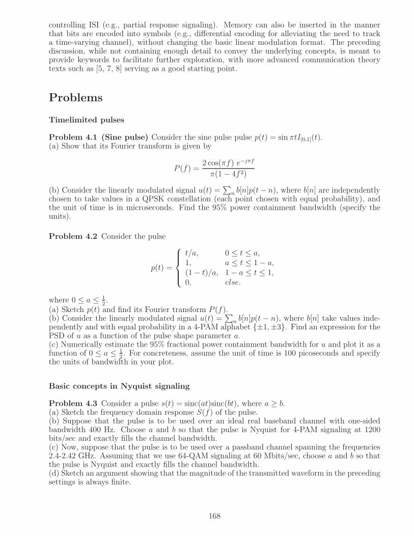
controlling ISI (e.g., partial response signaling). Memory can also be inserted in the mannerthat bits are encoded into symbols (e.g., differential encoding for alleviating the need to tracka time-varying channel), without changing the basic linear modulation format. The precedingdiscussion, while not containing enough detail to convey the underlying concepts, is meant toprovide keywords to facilitate further exploration, with more advanced communication theorytexts such as [5, 7, 8] serving as a good starting point.

Problems

Timelimited pulses

Problem 4.1 (Sine pulse) Consider the sine pulse pulse p(t) = sin πtI[0,1](t).(a) Show that its Fourier transform is given by

P (f) =2 cos(πf) e−jπf

π(1− 4f 2)

(b) Consider the linearly modulated signal u(t) =∑

n b[n]p(t− n), where b[n] are independentlychosen to take values in a QPSK constellation (each point chosen with equal probability), andthe unit of time is in microseconds. Find the 95% power containment bandwidth (specify theunits).

Problem 4.2 Consider the pulse

p(t) =

t/a, 0 ≤ t ≤ a,1, a ≤ t ≤ 1− a,(1− t)/a, 1− a ≤ t ≤ 1,0, else.

where 0 ≤ a ≤ 12.

(a) Sketch p(t) and find its Fourier transform P (f).(b) Consider the linearly modulated signal u(t) =

∑

n b[n]p(t − n), where b[n] take values inde-pendently and with equal probability in a 4-PAM alphabet ±1,±3. Find an expression for thePSD of u as a function of the pulse shape parameter a.(c) Numerically estimate the 95% fractional power containment bandwidth for u and plot it as afunction of 0 ≤ a ≤ 1

2. For concreteness, assume the unit of time is 100 picoseconds and specify

the units of bandwidth in your plot.

Basic concepts in Nyquist signaling

Problem 4.3 Consider a pulse s(t) = sinc(at)sinc(bt), where a ≥ b.(a) Sketch the frequency domain response S(f) of the pulse.(b) Suppose that the pulse is to be used over an ideal real baseband channel with one-sidedbandwidth 400 Hz. Choose a and b so that the pulse is Nyquist for 4-PAM signaling at 1200bits/sec and exactly fills the channel bandwidth.(c) Now, suppose that the pulse is to be used over a passband channel spanning the frequencies2.4-2.42 GHz. Assuming that we use 64-QAM signaling at 60 Mbits/sec, choose a and b so thatthe pulse is Nyquist and exactly fills the channel bandwidth.(d) Sketch an argument showing that the magnitude of the transmitted waveform in the precedingsettings is always finite.

168

Problem 4.4 Consider the pulse p(t) whose Fourier transform satisfies:

P (f) =

1, 0 ≤ |f | ≤ A

B−|f |B−A

, A ≤ |f | ≤ B

0, else

where A = 250KHz and B = 1.25MHz.(a) True or False The pulse p(t) can be used for Nyquist signaling at rate 3 Mbps using an8-PSK constellation.(b) True or False The pulse p(t) can be used for Nyquist signaling at rate 4.5 Mbps using an8-PSK constellation.

Problem 4.5 Consider the pulse

p(t) =

1− |t|T, 0 ≤ |t| ≤ T

0, else

Let P (f) denote the Fourier transform of p(t).(a) True or False The pulse p(t) is Nyquist at rate 1

T.

(b) True or False The pulse p(t) is square root Nyquist at rate 1T. (i.e., |P (f)|2 is Nyquist at

rate 1T).

P(f)

a b−b −a f

Figure 4.18: Signaling pulse for Problem 4.6.

Problem 4.6 Consider Nyquist signaling at 80 Mbps using a 16QAM constellation with 50%excess bandwidth. The signaling pulse has spectrum shown in Figure 4.18.(a) Find the values of a and b in the figure, making sure you specify the units.(b) True or False The pulse is also Nyquist for signaling at 20 Mbps using QPSK. (Justify youranswer.)

Problem 4.7 Consider linear modulation with a signaling pulse p(t) = sinc(at)sinc(bt), wherea and b are to be determined.(a) How should a and b be chosen so that p(t) is Nyquist with 50% excess bandwidth for a datarate of 40 Mbps using 16QAM? Specify the occupied bandwidth.(b) How should a and b be chosen so that p(t) can be used for Nyquist signaling both for a16QAM system with 40 Mbps data rate, and for an 8PSK system with 18 Mbps data rate?Specify the occupied bandwidth.

169

Problem 4.8 Consider a passband communication link operating at a bit rate of 16 Mbps usinga 256-QAM constellation.(a) What must we set the unit of time as so that p(t) = sin πtI[0,1](t) is square root Nyquist forthe system of interest, while occupying the smallest possible bandwidth?(b) What must we set the unit of time as so that p(t) = sinc(t)sinc(2t) is Nyquist for the systemof interest, while occupying the smallest possible bandwidth?

Problem 4.9 Consider passband linear modulation with a pulse of the form p(t) = sinc(3t)sinc(2t),where the unit of time is microseconds.(a) Sketch the spectrum P (f) versus f . Make sure you specify the units on the f axis.(b) What is the largest achievable bit rate for Nyquist signaling using p(t) if we employ a 16QAMconstellation? What is the fractional excess bandwidth for this bit rate?(c) (True or False) The pulse p(t) can be used for Nyquist signaling at a bit rate of 4 Mbpsusing a QPSK constellation.

Problem 4.10 (True or False) Any pulse timelimited to duration T is square root Nyquist(up to scaling) at rate 1/T .

Problem 4.11 (Raised cosine pulse) In this problem, we derive the time domain response ofthe frequency domain raised cosine pulse. Let R(f) = I[− 1

2, 12](f) denote an ideal boxcar transfer

function, and let C(f) = π2a

cos(πaf)I[− a

2, a2] denote a cosine transfer function.

(a) Sketch R(f) and C(f), assuming that 0 < a < 1.(b) Show that the frequency domain raised cosine pulse can be written as

S(f) = (R ∗ C)(f)

(c) Find the time domain pulse s(t) = r(t)c(t). Where are the zeros of s(t)? Conclude thats(t/T ) is Nyquist at rate 1/T .(d) Sketch an argument that shows that, if the pulse s(t/T ) is used for BPSK signaling at rate1/T , then the magnitude of the transmitted waveform is always finite.

Software experiments with Nyquist and square root Nyquist pulses

Problem 4.12 (Software exercise for the raised cosine pulse) Code fragment 4.B.1 in theappendix implements a discrete time truncated raised cosine pulse.(a) Run the code fragment for 25%, 50% and 100% excess bandwidths and plot the time domainwaveforms versus normalized time t/T over the interval [−5T, 5T ], sampling fast enough (e.g.,at rate 32/T or higher) to obtain smooth curves. Comment on the effect of varying the excessbandwidth on these waveforms.(b) For excess bandwidth of 50%, numerically explore the effect of time domain truncation onfrequency domain spillage. Specifically, compute the Fourier transform for two cases: truncationto [−2T, 2T ] and truncation to [−5T, 5T ], using the DFT as described in code fragment 2.5.1 toobtain a frequency resolution at least as good as 1

64T. Plot these Fourier transforms against the

normalized frequency fT , and comment on how much of increase in bandwidth, if any, you seedue to truncation in the two cases.(c) Numerically compute the 95% bandwidth of the two pulses in (b), and compare it with thenominal bandwidth without truncation.

Problem 4.13 (Software exercise for the SRRC pulse) (a) Write a function for generatinga sampled SRRC pulse, analogous to code fragment 4.B.1, where you can specify the sampling

170

rate, the excess bandwidth, and the truncation length. The time domain expression for theSRRC pulse is given by (4.45) in the appendix.Remark: The zero in the denominator can be handled either by analytical or numerical imple-mentation of L’Hospital’s rule. See comments in code fragment 4.B.1.(b) Plot the SRRC pulses versus normalized time t/T , for excess bandwidths of 25%, 50% and100%. Comment on the effect of varying excess bandwidth on these waveforms.(c) in the appendix implements a discrete time truncated raised cosine pulse.(a) Run the code fragment for 25%, 50% and 100% excess bandwidths and plot the time domainwaveforms over [−5T, 5T ], sampling fast enough (e.g., at rate 32/T or higher) to obtain smoothcurves. Comment on the effect of varying the excess bandwidth on these waveforms.(b) For excess bandwidth of 50%, numerically explore the effect of time domain truncation onfrequency domain spillage. Specifically, compute the Fourier transform for two cases: truncationto [−2T, 2T ] and truncation to [−5T, 5T ], using the DFT as described in code fragment 2.5.1 toobtain a frequency resolution at least as good as 1

64T. Plot these Fourier transforms against the

normalized frequency fT , and comment on how much of increase in bandwidth, if any, you seedue to truncation in the two cases.(c) Numerically compute the 95% bandwidth of the two pulses in (b), and compare it with thenominal bandwidth without truncation.

Effect of timing errors

Problem 4.14 (Effect of timing errors) Consider digital modulation at rate 1/T using thesinc pulse s(t) = sinc(2Wt), with transmitted waveform

y(t) =

100∑

n=1

bns(t− (n− 1)T )

where 1/T is the symbol rate and bn is the bit stream being sent (assume that each bn takesone of the values ±1 with equal probability). The receiver makes bit decisions based on thesamples rn = y((n− 1)T ), n = 1, ..., 100.(a) For what value of T (as a function of W ) is rn = bn, n = 1, ..., 100?Remark: In this case, we simply use the sign of the nth sample rn as an estimate of bn.(b) For the choice of T as in (a), suppose that the receiver sampling times are off by .25 T. Thatis, the nth sample is given by rn = y((n−1)T + .25T ), n = 1, ..., 100. In this case, we do have ISIof different degrees of severity, depending on the bit pattern. Consider the following bit pattern:

bn =

(−1)n−1 1 ≤ n ≤ 49(−1)n 50 ≤ n ≤ 100

Numerically evaluate the 50th sample r50. Does it have the same sign as the 50th bit b50?Remark: The preceding bit pattern creates the worst possible ISI for the 50th bit. Since the sincpulse dies off slowly with time, the ISI contributions due to the 99 other bits to the 50th samplesum up to a number larger in magnitude, and opposite in sign, relative to the contribution dueto b50. A decision on b50 based on the sign of r50 would therefore be wrong. This sensitivity totiming error is why the sinc pulse is seldom used in practice.(c) Now, consider the digitally modulated signal in (a) with the pulse s(t) = sinc(2Wt)sinc(Wt).For ideal sampling as in (a), what are the two values of T such that rn = bn?(d) For the smaller of the two values of T found in (c) (which corresponds to faster signaling,since the symbol rate is 1/T ), repeat the computation in (b). That is, find r50 and compare itssign with b50 for the bit pattern in (b).(e) Find and sketch the frequency response of the pulse in (c). What is the excess bandwidthrelative to the pulse in (a), assuming Nyquist signaling at the same symbol rate?(f) Discuss the impact of the excess bandwidth on the severity of the ISI due to timing mismatch.

171

−1 1 3−3

3

1

−3

−1

Figure 4.19: 16QAM constellation with scaling chosen for convenient computation of powerefficiency.

Power-bandwidth tradeoffs

Problem 4.15 (Power efficiency of 16QAM) In this problem, we sketch the computationof power efficiency for the 16QAM constellation shown in Figure 4.19.(a) Note that the minimum distance for the particular scaling chosen in the figure is dmin = 2.(b) Show that the constellation points divide into 3 categories based on their distance from theorigin, corresponding to squared distances, or energies, of 12+12, 12+32 and 32+32. Averagingover these energies (weighting by the number of points in each category), show that the averageenergy per symbol is Es = 10.(c) Using (a) and (b), and accounting for the number of bits/symbol, show that the power

efficiency is given by ηP =d2min

Eb= 8

5.

Problem 4.16 (Power-bandwidth tradeoffs) A 16QAM system transmits at 50 Mbps usingan excess bandwidth of 50%. The transmit power is 100 mW.(a) Assuming that the carrier frequency is 5.2 GHz, specify the frequency interval occupied bythe passband modulated signal.(b) Using the same frequency band in (a), how fast could you signal using QPSK with the sameexcess bandwidth?(c) Estimate the transmit power needed in the QPSK system, assuming the same range andreliability requirements as in the 16QAM system.

Minimum Shift Keying

Problem 4.17 (OQPSK and MSK) Linear modulation with a bandlimited pulse can performpoorly over nonlinear passband channels. For example, the output of a passband hardlimiter(which is a good model for power amplifiers operating in a saturated regime) has constantenvelope, but a PSK signal employing a bandlimited pulse has an envelope that passes throughzero during a 180 degree phase transition, as shown in Figure 4.20. One way to alleviate thisproblem is to not allow 180 degree phase transitions. Offset QPSK (OQPSK) is one example ofsuch a scheme, where the transmitted signal is given by

s(t) =

∞∑

n=−∞bc[n]p(t− nT ) + jbs[n]p(t− nT − T

2) (4.26)

where bc[n], bs[n] are ±1 BPSK symbols modulating the I and Q channels, with the I and Qsignals being staggered by half a symbol interval. This leads to phase transitions of at most 90

172

Envelope is zero due to 180 degrees phase transition

Figure 4.20: The envelope of a PSK signal passes through zero during a 180 degree phasetransition, and gets distorted over a nonlinear channel.

degrees at integer multiples of the bit time Tb =T2. Minimum Shift Keying (MSK) is a special

case of OQPSK with timelimited modulating pulse

p(t) =√2 sin(

πt

T)I[0,T ](t) (4.27)

(a) Sketch the I and Q waveforms for a typical MSK signal, clearly showing the timing relationshipbetween the waveforms.(b) Show that the MSK waveform has constant envelope (an extremely desirable property fornonlinear channels).(c) Find an analytical expression for the PSD of an MSK signal, assuming that all bits sent arei.i.d., taking values ±1 with equal probability. Plot the PSD versus normalized frequency fT .(d) Find the 99% power containment normalized bandwidth of MSK. Compare with the minimumNyquist bandwidth, and the 99% power containment bandwidth of OQPSK using a rectangularpulse.(e) Recognize that Figure 4.6 gives the PSD for OQPSK and MSK, and reproduce this figure,normalizing the area under the PSD curve to be the same for both modulation formats.

Orthogonal signaling

Problem 4.18 (FSK tone spacing) Consider two real-valued passband pulses of the form

s0(t) = cos(2πf0t+ φ0) 0 ≤ t ≤ Ts1(t) = cos(2πf1t+ φ1) 0 ≤ t ≤ T

where f1 > f0 ≫ 1/T . The pulses are said to be orthogonal if 〈s0, s1〉 =∫ T

0s0(t)s1(t)dt = 0.

(a) If φ0 = φ1 = 0, show that the minimum frequency separation such that the pulses areorthogonal is f1 − f0 =

12T.

(b) If φ0 and φ1 are arbitrary phases, show that the minimum separation for the pulses to beorthogonal regardless of φ0, φ1 is f1 − f0 = 1/T .Remark: The results of this problem can be used to determine the bandwidth requirements forcoherent and noncoherent FSK, respectively.

Problem 4.19 (Walsh-Hadamard codes)(a) Specify the Walsh-Hadamard codes for 8-ary orthogonal signaling with noncoherent reception.(b) Plot the baseband waveforms corresponding to sending these codes using a square root raisedcosine pulse with excess bandwidth of 50%.(c) What is the fractional increase in bandwidth efficiency if we use these 8 waveforms as buildingblocks for biorthogonal signaling with coherent reception?

173

t

0 2 0 1 2

1 1

−1

a(t) b(t)

t

Figure 4.21: Baseband signals for Problem 4

Problem 4.20 The two orthogonal baseband signals shown in Figure 4.21 are used as buildingblocks for constructing passband signals as follows.

up(t) = a(t) cos 2πfct− b(t) sin 2πfctvp(t) = b(t) cos 2πfct− a(t) sin 2πfctwp(t) = b(t) cos 2πfct+ a(t) sin 2πfctxp(t) = a(t) cos 2πfct+ b(t) sin 2πfct

where fc ≫ 1.(a) True or False The signal set can be used for 4-ary orthogonal modulation with coherentdemodulation.(b) True or False The signal set can be used for 4-ary orthogonal modulation with noncoherentdemodulation.

Bandwidth occupancy as a function of modulation format

Problem 4.21 We wish to send at a rate of 10 Mbits/sec over a passband channel. Assum-ing that an excess bandwidth of 50% is used, how much bandwidth is needed for each of thefollowing schemes: QPSK, 64-QAM, and 64-ary noncoherent orthogonal modulation using aWalsh-Hadamard code.

Problem 4.22 Consider 64-ary orthogonal signaling using Walsh-Hadamard codes. Assumingthat the chip pulse is square root raised cosine with excess bandwidth 25%, what is the bandwidthrequired for sending data at 20 Kbps over a passband channel assuming (a) coherent reception,(b) noncoherent reception.

Software Lab 4.1: Linear modulation over a noiseless ideal channel

This is the first of a sequence of software labs which gradually develop a reasonably completeMatlab simulator for a linearly modulated system. (the follow-on labs are in Chapters 6 and 7)

Background

Figure 4.22 shows block diagrams corresponding to a typical DSP-centric realization of a com-munication transceiver employing linear modulation. In the labs, we model the core componentsof such a system using the complex baseband representation, as shown in Figure 4.23. Given theequivalence of passband and complex baseband, we are only skipping the modeling of finite pre-cision effects due to digital-to-analog conversion (DAC) and analog-to-digital conversion (ADC).

174

demodulation)

Transmitfilter(implementedat rate 4/T)

I

Q

Digitalstreamsrate 4/T

Analog

I

QDnconverter

ADC

ADC

filter(implementedat rate 4/T)

DSP for

receiver

functions

(includes coarse analogpassband filtering)

Upconverter

Two−dimensionalsymbols

rate 1/T

I

Q

Digitalstreamsrate 4/T

DAC

DACI

Q

waveformsbasebandAnalog

symbols

Estimated

waveformsbaseband

PassbandChannel

Receive

(synchronization,equalization,

Figure 4.22: Typical DSP-centric transceiver realization. Our model does not include the blocksshown in dashed lines. Finite precision effects such as DAC and ADC are not considered. Theupconversion and downconversion operations are not modeled. The passband channel is modeledas an LTI system in complex baseband.

Estimated

TX

Transmit

Filter

Cg (t)

ChannelFilter

g (t)RX

ReceiveFilterb[n]

Noise

Rate 1/T

Sampler,rate m/T

ProcessingSignal

Receiver

(Synchronization,Equalization,Demodulation)

Symbols

symbolsg (t)

Figure 4.23: Block diagram of a linearly modulated system, modeled in complex baseband.

175

These effects can easily be incorporated into Matlab models such as those we develop, but arebeyond our current scope.

A few points worth noting about the model of Figure 4.23:

Choice of transmit filter: The PSD of the transmitted signal is proportional to |GTX(f)|2 (seeChapter 4). The choice of transmit filter is made based on spectral constraints, as well as con-siderations such as sensitivity to receiver timing errors and intersymbol interference. Typically,the bandwidth employed is of the order of 1

T.

Channel model: We typically model the channel as an linear time-invariant (LTI) system. Forcertain applications, such as wireless communications, the channel may be modeled as slowlytime varying.

Noise model: Noise is introduced in a later lab (in Chapter 6).

Receive filter and sampler: The optimal choice of receive filter is actually a filter matched tothe cascade of the transmit filter and the channel. In this case, there is no information lossin sampling the output of the receive filter at the symbol rate 1

T. Often, however, we use a

suboptimal choice of receive filter (e.g., a wideband filter flat over the signal band, or a filtermatched to the transmit filter). In this case, it is typically advantageous to sample faster thanthe symbol rate. In general, we assume that the sampler operates at rate m

T, where m is a positive

integer. The output of the sampler is then processed, typically using digital signal processing(DSP), to perform receiver functions such as synchronization, equalization and demodulation..

The simulation of a linearly modulated system typically involves the following steps.

Step 1: Generating random symbols to be sent

We restrict attention in this lab to Binary Phase Shift Keying (BPSK). That is, the symbolsbn in Figure 1 take values ±1.

Step 2: Implementing the transmit, channel, and receive filters

Since the bandwidth of these filters is of the order of 1T, they can be accurately implemented in

DSP by using FIR filters operating on samples at a rate which is a suitable multiple of 1T. The

default choice of sampling rate in the labs is 4T, unless specified otherwise. If the filter is specified

in continuous time, typically, one simply samples the impulse response at rate 4T, taking a large

enough filter length to capture most of the energy in the impulse response. Code fragment 4.B.1in the appendix illustrates generating a discrete time filter corresponding to a truncated raisedcosine pulse.

Step 3: Sending the symbols through the filters.

To send symbols at rate 1T

through filters implemented at rate 4T, it is necessary to upsample

the symbols before convolving them with the filter impulse response determined in Step 2. Codefragment 4.B.2 in the appendix illustrates this for a raised cosine pulse.

Step 4: Adding noise

Typically, we add white Gaussian noise (model to be specified in a later lab) at the input to thereceive filter.

Step 5: Processing at the receive filter output

If there is no intersymbol interference (ISI), the processing simply consists of sampling at rate 1T

to get decision statistics for the symbols of interest. For BPSK, you might simply take the signof the decision statistic to make your bit decision.

If the ISI is significant, then channel equalization (discussed in a later lab) is required prior tomaking symbol decisions.

Laboratory Assignment

176

See Appendix 4.B for information that may be useful for this lab.

0) Write a Matlab function analogous to Code Fragment 4.B.1 to generate an SRRC pulse (i.e.,do Problem 4.13(a)) where you can specify the truncation length and the excess bandwidth.

1) Set the transmit filter to an SRRC pulse with excess bandwidth 22%, sampled at rate 4/Tand truncated to [−5T, 5T ]. Plot the impulse response of the transmit filter versus t/T .

If you have difficulty generating the SRRC pulse, use the following code fragment to generatethe transmit filter:

Code Fragment 4.7.1 (Explicit specification of transmit filter)

%first specify half of the filterhhalf = [-0.025288315;-0.034167931;-0.035752323;-0.016733702;0.021602514;0.064938487;0.091002137;0.081894974;0.037071157;-0.021998074;-0.060716277 ;-0.051178658;0.007874526;0.084368728;0.126869306;0.094528345;-0.012839661;-0.143477028;-0.211829088;-0.140513128;0.094601918;0.441387140;0.785875640;1.0];transmit_filter = [hhalf;flipud(hhalf)];

2) Using the DFT (as in Code Fragment 2.5.1 for Example 2.5.4), compute the magnitude ofthe transfer function of the transmit filter versus the normalized frequency fT (make sure theresolution in frequency is good enough to get a smooth plot, e.g., at least as good as 1

64T). From

eyeballing the plot, check whether the normalized bandwidth (i.e., bandwidth as a multiple of1T) is well predicted by the nominal excess bandwidth.

3) Use the transmit filter in the Code Fragment 4.B.2, which implements upsampling and allowssending a programmable number of symbols through the system. Set the receive filter to be thematched filter corresponding to the transmit filter, and plot the response at the output of thereceive filter to a single symbol. Is the cascade of the transmit and receive filters is Nyquist atrate 1/T ?

4) Generate 100 random bits a[n] taking values in 0, 1, and map them to symbols b[n]taking values in −1,+1, with 0 mapped to +1 and 1 to −1.

5) Send the 100 symbols b[n] through the system. What is the length of the correspondingoutput of the transmit filter? What is the length of the corresponding output of the receivefilter? Plot separately the input to the receive filter, and the output of the receive filter versustime, with one unit of time on the x-axis equal to the symbol time T .

6) Do the best job you can in recovering the transmitted bits a[n] by directly sampling theinput to the receive filter, and add lines in the matlab code for implementing your idea. Thatis, select a set of 100 samples, and estimate the 100 transmitted bits based on the sign of thesesamples. (What sampling delay and spacing would you use?). Estimate the probability of error(note: no noise has been added).

7) Do the best job you can in recovering the transmitted bits by directly sampling the output ofthe receive filter, and add lines in the Matlab code for implementing your idea. That is, select aset of 100 samples, estimate the 100 transmitted bits based on the sign of these samples. (Whatsampling delay and spacing would you use?). Estimate the probability of error. Also estimatethe probability of error if you chose an incorrect delay, offset from the correct delay by T/2.

8) Suppose that the receiver LO used for downconversion is ahead in frequency and phase relativeto the incoming wave by ∆f = 1

40Tand a phase of π/2. Modify your complex baseband model

to include the effects of the carrier phase and frequency offset. When you now sample at the“correct” delay as determined in 7), do a scatter plot of the complex-valued samples y[n], n =1, ..., 100 that you obtain. Can you make correct decisions based on taking the sign of the realpart of the samples, as in 7)?

177

9) Now consider a differentially encoded system in which we send a[n], n = 1, ..., 99, wherea[n]∈0, 1, by sending the following ±1 bits: b[1] = +1, and for n = 2, ..., 100

b[n] =

b[n− 1], a[n] = 0,−b[n− 1], a[n] = 1,

Devise estimates for the bits a[n] from the samples y[n] in 8), and estimate the probabilityof error.Hint: What does y[n]y∗[n− 1] look like?

Lab Report: Your lab report should answer the preceding questions in order, and should documentthe reasoning you used and the difficulties you encountered. Comment on whether you get bettererror probability in 6) or 7), and why?

4.A Power spectral density of a linearly modulated signal

We wish to compute the PSD of a linearly modulated signal of the form

u(t) =∑

n

b[n]p(t− nT )

While we model the complex-valued symbol sequence b[n] as random, we do not need toinvoke concepts from probability and random processes to compute the PSD, but can simplymodel time-averaged quantities for the symbol sequence. For example, the DC value, which istypically designed to be zero, is defined by

b[n] = limN→∞

1

2N + 1

N∑

n=−N

b[n] (4.28)

We also define the time-averaged autocorrelation function Rb[k] = b[n]b∗[n− k] for the symbolsequence as the following limit:

Rb[k[= limN→∞

1

2N

N∑

n=−N

b[n]b∗[n− k] (4.29)

Note that we are being deliberately sloppy about the limits of summation in n on the right-handside to avoid messy notation. Actually, since −N ≤ m = n − k ≤ N , we have the constraint−N + k ≤ n ≤ N + k in addition to the constraint −N ≤ n ≤ N . Thus, the summation inn should depend on the delay k at which we are evaluating the autocorrelation function, goingfrom n = −N to n = N + k for k < 0, and n = −N + k to n = N for k ≥ 0. However, we ignorethese edge effects, since become negligible when we let N get large while keeping k fixed.

We now compute the time-averaged PSD. As described in Section 4.2.1, the steps for computingthe PSD for a finite-power signal u(t) are as follows:(a) timelimit to a finite observation interval of length To to get a finite energy signal uTo(t);(b) compute the Fourier transform UTo(f), and hence obtain the energy spectral density |UTo(f)|2;(c) estimate the PSD as Su(f) =

|UTo (f)|2T0

, and take the limit T0 → ∞ to obtain Su(f).

Consider the observation interval [−NT,NT ], which fits roughly 2N symbols. In general, themodulation pulse p(t) need not be timelimited to the symbol duration T . However, we can

178

neglect the edge effects caused by this, since we eventually take the limit as the observationinterval gets large. Thus, we can write

uTo(t) ≈N∑

n=−N

b[n]p(t − nT )

Taking the Fourier transform, we obtain

UTo(f) =N∑

n=−N

b[n]P (f)e−j2πfnT

The energy spectral density is therefore given by

|UTo(f)|2 = UTo(f)U∗To(f) =

N∑

n=−N

b[n]P (f)e−j2πfnTN∑

m=−N

b∗[m]P ∗(f)ej2πfmT

where we need to use two different dummy variables, n and m, for the summations correspondingto UTo(f) and U

∗To(f), respectively. Thus,

|UTo(f)|2 = |P (f)|2N∑

m=−N

N∑

n=−N

b[n]b∗[m]e−j2π(m−n)fT

and the PSD is estimated as

Su(f) =|UTo(f)|22NT

=|P (f)|2T

1

2N

N∑

m=−N

N∑

n=−N

b[n]b∗[m]e−j2πf(n−m)T (4.30)

Thus, the PSD factors into two components: the first is a term |P (f)|2T

that depends only on thespectrum of the modulation pulse p(t), while the second term (in curly brackets) depends onlyon the symbol sequence b[n]. Let us now work on simplifying the latter. Grouping terms ofthe form m = n− k for each fixed k, we can rewrite this term as

1

2N

N∑

m=−N

N∑

n=−N

b[n]b∗[m]e−j2πf(n−m)T =∑

k

1

2N

N∑

n=−N

b[n]b∗[n− k]e−j2πfkT (4.31)

From (4.29), we see that taking the limit N → ∞ in (4.31) yields∑

k Rb[k]e−j2πfkT . Substituting

into (4.30), we obtain that the PSD is given by

Su(f) =|P (f)|2T

∑

k

Rb[k]e−j2πfkT (4.32)

Thus, we see that the PSD depends both on the modulating pulse p(t) and on the propertiesof the symbol sequence b[n]. We explore how the dependence on the symbol sequence canbe exploited for shaping the spectrum in the problems. However, for most systems, the symbolsequence can be modeled as uncorrelated and zero mean, In this case, Rb[k] = 0 for k 6= 0.Specializing to this important setting yields Theorem 4.2.1.

179

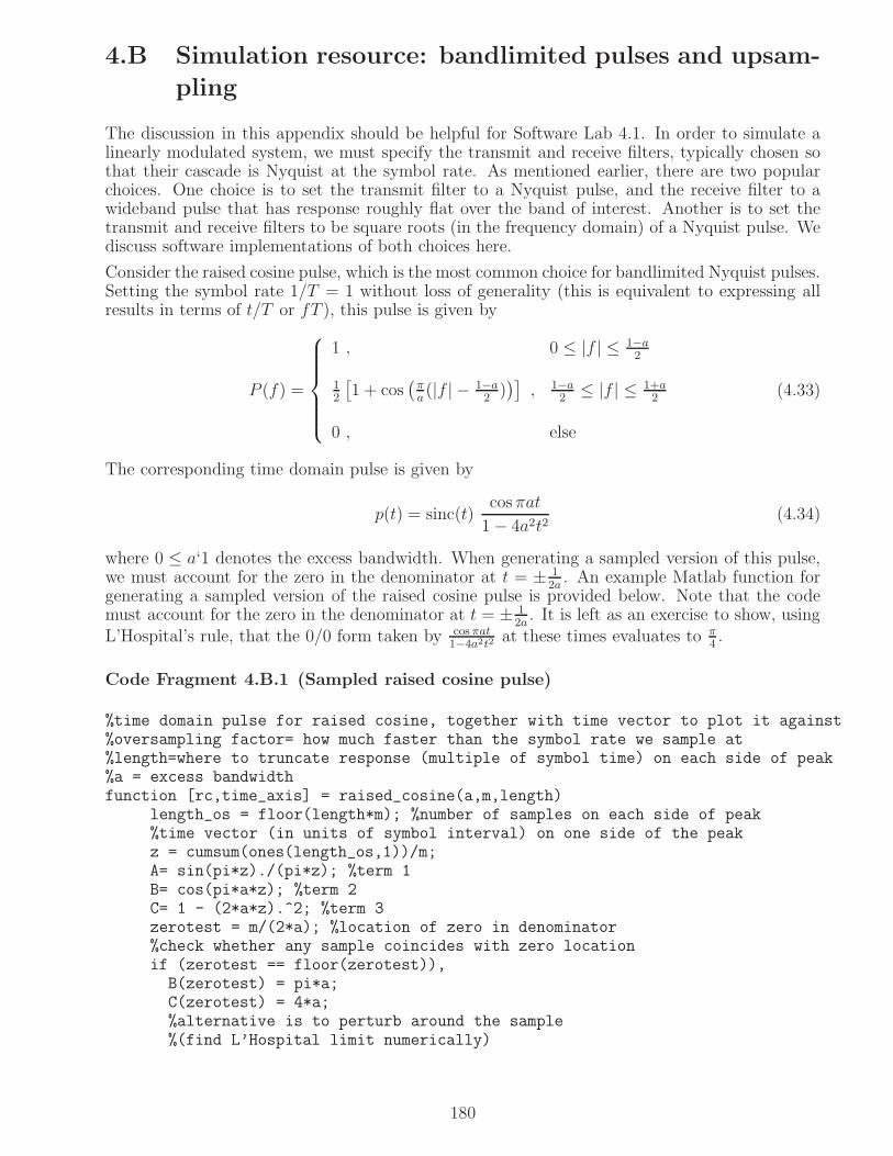
4.B Simulation resource: bandlimited pulses and upsam-

pling

The discussion in this appendix should be helpful for Software Lab 4.1. In order to simulate alinearly modulated system, we must specify the transmit and receive filters, typically chosen sothat their cascade is Nyquist at the symbol rate. As mentioned earlier, there are two popularchoices. One choice is to set the transmit filter to a Nyquist pulse, and the receive filter to awideband pulse that has response roughly flat over the band of interest. Another is to set thetransmit and receive filters to be square roots (in the frequency domain) of a Nyquist pulse. Wediscuss software implementations of both choices here.

Consider the raised cosine pulse, which is the most common choice for bandlimited Nyquist pulses.Setting the symbol rate 1/T = 1 without loss of generality (this is equivalent to expressing allresults in terms of t/T or fT ), this pulse is given by

P (f) =

1 , 0 ≤ |f | ≤ 1−a2

12

[

1 + cos(

πa(|f | − 1−a

2))]

, 1−a2

≤ |f | ≤ 1+a2

0 , else

(4.33)

The corresponding time domain pulse is given by

p(t) = sinc(t)cosπat

1− 4a2t2(4.34)

where 0 ≤ a‘1 denotes the excess bandwidth. When generating a sampled version of this pulse,we must account for the zero in the denominator at t = ± 1

2a. An example Matlab function for

generating a sampled version of the raised cosine pulse is provided below. Note that the codemust account for the zero in the denominator at t = ± 1

2a. It is left as an exercise to show, using

L’Hospital’s rule, that the 0/0 form taken by cos πat1−4a2t2

at these times evaluates to π4.

Code Fragment 4.B.1 (Sampled raised cosine pulse)

%time domain pulse for raised cosine, together with time vector to plot it against%oversampling factor= how much faster than the symbol rate we sample at%length=where to truncate response (multiple of symbol time) on each side of peak%a = excess bandwidthfunction [rc,time_axis] = raised_cosine(a,m,length)

length_os = floor(length*m); %number of samples on each side of peak%time vector (in units of symbol interval) on one side of the peakz = cumsum(ones(length_os,1))/m;A= sin(pi*z)./(pi*z); %term 1B= cos(pi*a*z); %term 2C= 1 - (2*a*z).^2; %term 3zerotest = m/(2*a); %location of zero in denominator%check whether any sample coincides with zero locationif (zerotest == floor(zerotest)),

B(zerotest) = pi*a;C(zerotest) = 4*a;%alternative is to perturb around the sample%(find L’Hospital limit numerically)

180

%B(zerotest) = cos(pi*a*(zerotest+0.001));%C(zerotest) = 1-(2*a*(zerotest+0.001))^2

endD = (A.*B)./C; %response to one side of peakrc = [flipud(D);1;D]; %add in peak and other sidetime_axis = [flipud(-z);0;z];

This can, for example, be used to generate a plot of the raised cosine pulse, as follows, where wewould typically oversample by a large factor (e.g., m = 32) in order to get a smooth plot.

%%plot time domain raised cosine pulsea = 0.5; % desired excess bandwidthm = 32; %oversample by a lot to get smooth plotlength = 10; % where to truncate the time domain response (one-sided, multiple of symbol time)[rc,time] = raised_cosine(a,M,length);plot(time,rc);

The code for the raised cosine function can also be used to generate the coefficients of a dis-crete time transmit filter. Here, the oversampling factor would be dictated by our DSP-centricimplementation, and would usually be far less than what is required for a smooth plot: thedigital-to-analog converter would perform the interpolation required to provide a smooth analogwaveform for upconversion. A typical choice ism = 4, as in the Matlab code below for generatinga noiseless BPSK modulated signal.

Upsampling: As noted in our preview of digital modulation in Section 2.3.2, the symbols comein every T seconds, while the samples of the transmit filter are spaced by T/m. For example,the nth symbol contributes b[n]p(t− nT ) to the transmit filter output, and the (n+1)st symbolcontributes b[n + 1]p(t − (n + 1)T ). Since p(t − nT ) and p(t − (n + 1)T ) are offset by T , theymust be offset by m samples when sampling at a rate of m/T . Thus, if the symbols are input toa transmit filter whose discrete time impulse response is expressed at sampling rate m/T , thensuccessive symbols at the input to the filter must be spaced by m samples. That is, in order toget the output as a convolution of the symbols with the transmit filter expressed at rate m/T ,we must insert m − 1 zeros between successive symbols to convert them to a sampling rate ofm/T .

For completeness, we reproduce part of the upsampling Code Fragment 2.3.2 below in imple-menting a raised cosine transmit filter.

Code Fragment 4.B.2 (Sampled transmitter output)

oversampling_factor = 4;m = oversampling_factor;%parameters for sampled raised cosine pulsea = 0.5;length = 10;% (truncated outside [-length*T,length*T])%raised cosine transmit filter (time vector set to a dummy variable which is not used)[transmit_filter,dummy] = raised_cosine(a,m,length);%NUMBER OF SYMBOLSnsymbols = 100;%BPSK SYMBOL GENERATIONsymbols = sign(rand(nsymbols,1) -.5);%UPSAMPLE BY mnsymbols_upsampled = 1+(nsymbols-1)*m;%length of upsampled symbol sequencesymbols_upsampled = zeros(nsymbols_upsampled,1);%initialize

181

symbols_upsampled(1:m:nsymbols_upsampled)=symbols;%insert symbols with spacing m%NOISELESS MODULATED SIGNALtx_output = conv(symbols_upsampled,transmit_filter);

Let us now discuss the implementation of an alternative transmit filter, the square root raisedcosine (SRRC). The frequency domain SRRC pulse is given by G(f) =

√

P (f), where P (f) isas in (4.33). We now need to find a sampled version of the time domain pulse g(t) in order toimplement linear modulation as above. While this could be done numerically by sampling thefrequency domain pulse and computing an inverse DFT, we can also find an analytical formulafor g(t), as follows. Given the practical importance of the SRRC pulse, we provide the formulaand sketch its derivation. Noting that 1 + cos theta = 2 cos2 θ, we can rewrite the frequencydomain expression (4.33) for the raised cosine pulse as

P (f) =

1 , 0 ≤ |f | ≤ 1−a2

cos2(

π2a(|f | − 1−a

2))

, 1−a2

≤ |f | ≤ 1+a2

0 , else

(4.35)

We can now take the square root to get an analytical expression for the SRRC pulse in thefrequency domain as follows:

G(f) =

1 , 0 ≤ |f | ≤ 1−a2

cos(

π2a(|f | − 1−a

2))

, 1−a2

≤ |f | ≤ 1+a2

0 , else

Frequency domain SRRC pulse

(4.36)Finding the time domain SRRC pulse is now a matter of computing the inverse Fourier transform.Since it is also an interesting exercise in utilizing Fourier transform properties, we sketch thederivation. First, we break up the frequency domain pulse into segments whose inverse Fouriertransforms are well known. Setting b = 1−a

2, we have

G(f) = G1(f) +G2(f) (4.37)

where

G1(f) = I[−b,b](f) ↔ g1(t) = 2b sinc(2bt) =sin(2πbt)

πt=

sin π(1− a)t

πt(4.38)

andG2(f) = U(f − b) + U(−f − b) (4.39)

with

U(f) = cos( π

2af)

I[0,a](f) =1

2

(

ejπ2a

f + e−j π2a

f)

I[0,a](f) (4.40)

To evaluate g2(t), note first that

I[0,a](f) ↔= a sinc(at) ejπat (4.41)

Multiplication by ejπ2a

f in the frequency domain corresponds to leftward time shift by 14a, while

multiplication by e−j π2a

f corresponds to a rightward time shift by 14a. From (4.40) and (4.41), we

therefore obtain that

U(f) = cos( π

2af)

I[0,a](f) ↔ u(t) =a

2sinc

(

a(t +1

4a)

)

ejπa(t+14a

)+a

2sinc

(

a(t− 1

4a)

)

ejπa(t−14a

)

182

Simplifying, we obtain that

u(t) =a

π

2ej2πat − j8at

1− 16a2t2(4.42)

Now,

G2(f) = U(f − b) + U(−f − b) ↔ g2(t) = u(t)ej2πbt + u∗(t)e−j2πbt = Re(

2u(t)ej2πbt)

(4.43)

Plugging in (4.42), and substituting the value of b = 1−a2, we obtain upon simplification that

2u(t)ej2πbt =2a

π

2ejπ(1+a)t − j8atejπ(1−a)t

1− 16a2t2

Taking the real part, we obtain

g2(t) =1

π

4a cos(π(1 + a)t) + 16a2t sin(π(1− a)t)

1− 16a2t2(4.44)

Combining (4.38) and (4.44) and simplifying, we obtain the following expression for the SRRCpulse g(t) = g1(t) + g2(t):

g(t) =4a cos(π(1 + a)t) + sin(π(1−a)t)

t

π(1− 16a2t2)Time domain SRRC pulse (4.45)

We leave it as an exercise to write Matlab code to generate a sampled version of the SRRC pulse(analogous to Code Fragment 4.B.1), taking into account the zeros in the denominator. Thiscan then be used to generate a noiseless transmit waveform as in Code Fragment 4.B.2 simplyby replacing the transmit filter by an SRRC pulse.

183

Chapter 5

Probability and Random Processes

Probability theory is fundamental to communication system design, especially for digital commu-nication. Not only are there uncontrolled sources of uncertainty such as noise, interference, andother channel impairments that are only amenable to statistical modeling, but the very notion ofinformation underlying digital communication is based on uncertainty. In particular, the receiverin a communication system does not know a priori what the transmitter is sending (otherwisethe transmission would be pointless), hence the receiver designer must employ statistical modelsfor the transmitted signal. In this chapter, we review basic concepts of probability and randomvariables with examples motivated by communications applications. We also introduce the con-cept of random processes, which are used to model both signals and noise in communicationsystems.

Chapter Plan: The goal of this chapter is to develop the statistical modeling tools required inlater chapters. Sections 5.1 through 5.5 provide a review of background material on probabilityand random variables. Section 5.1 discusses basic concepts of probability: the most importantof these for our purpose are the concepts of conditional probability and Bayes’ rule. Sections 5.2and 5.4 discuss random variables and functions of random variables. Multiple random variables,or random vectors, are discussed in Section 5.3. Section 5.5 discusses various statistical averagesand their computation. Material which is not part of the assumed background starts with Section5.6; this section goes in depth into Gaussian random variables and vectors, which play a criticalrole in the mathematical modeling of communication systems. Section 5.7 introduces randomprocesses in sufficient depth that we can describe, and perform elementary computations with,the classical white Gaussian noise (WGN) model in Section 5.8. At this point, zealous followersof a “just in time” philosophy can move on to the discussion of optimal receiver design in Chapter6. However, many others might wish to go through one more section Section 5.9, which providesa more general treatment of the effect of linear operations on random processes. The results inthis section allow us, for example, to model noise correlations and to compute quantities such assignal-to-noise ratio (SNR). Material which we do not build on in later chapters, but which may beof interest to some readers, is placed in the appendices: this includes limit theorems, qualitativediscussion of noise mechanisms, discussion of the structure of passband random processes, andquantification, via SNR computations, of the effect of noise on analog modulation.

5.1 Probability Basics

In this section, we remind ourselves of some important definitions and properties.

Sample Space: The starting point in probability is the notion of an experiment whose outcomeis not deterministic. The set of all possible outcomes from the experiment is termed the samplespace Ω. For example, the sample space corresponding to the throwing of a six-sided die is

185

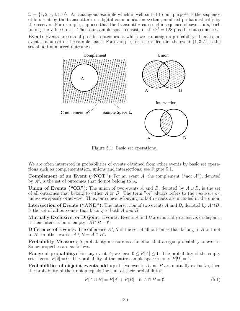
Ω = 1, 2, 3, 4, 5, 6. An analogous example which is well-suited to our purpose is the sequenceof bits sent by the transmitter in a digital communication system, modeled probabilistically bythe receiver. For example, suppose that the transmitter can send a sequence of seven bits, eachtaking the value 0 or 1. Then our sample space consists of the 27 = 128 possible bit sequences.

Event: Events are sets of possible outcomes to which we can assign a probability. That is, anevent is a subset of the sample space. For example, for a six-sided die, the event 1, 3, 5 is theset of odd-numbered outcomes.

c

BA

Union

A B

Intersection

Complement

A

Complement Sample SpaceA Ω

Figure 5.1: Basic set operations.

We are often interested in probabilities of events obtained from other events by basic set opera-tions such as complementation, unions and intersections; see Figure 5.1.

Complement of an Event (“NOT”): For an event A, the complement (“not A”), denotedby Ac, is the set of outcomes that do not belong to A.

Union of Events (“OR”): The union of two events A and B, denoted by A ∪ B, is the setof all outcomes that belong to either A or B. The term ”or” always refers to the inclusive or,unless we specify otherwise. Thus, outcomes belonging to both events are included in the union.

Intersection of Events (“AND”): The intersection of two events A and B, denoted by A∩B,is the set of all outcomes that belong to both A and B.

Mutually Exclusive, or Disjoint, Events: Events A andB are mutually exclusive, or disjoint,if their intersection is empty: A ∩ B = ∅.Difference of Events: The difference A \B is the set of all outcomes that belong to A but notto B. In other words, A \B = A ∩ Bc.

Probability Measure: A probability measure is a function that assigns probability to events.Some properties are as follows.

Range of probability: For any event A, we have 0 ≤ P [A] ≤ 1. The probability of the emptyset is zero: P [∅] = 0. The probabilty of the entire sample space is one: P [Ω] = 1.

Probabilities of disjoint events add up: If two events A and B are mutually exclusive, thenthe probability of their union equals the sum of their probabilities.

P [A ∪B] = P [A] + P [B] if A ∩ B = ∅ (5.1)

186

By mathematical induction, we can infer that the probability of the union of a finite number ofpairwise disjoint events also adds up. It is useful to review the principle of mathematical inductionvia this example. Specifically, suppose that we are given pairwise disjoint events A1, A2, A3, ....We wish to prove that, for any n ≥ 2,

P [A1 ∪ A2 ∪ ... ∪ An] = P [A1] + ...+ P [An] if Ai ∩ Aj = ∅ for all i 6= j (5.2)

Mathematical induction consists of the following steps:(a) verify that the result is true for the initial value of n, which in our case is n = 2;(b) assume that the result is true for an arbitrary value of n = k;(c) use (a) and (b) to prove that the result is true for n = k + 1.In our case, step (a) does not require any work; it holds by virtue of our assumption of (5.1).Now, assume that (5.2) holds for n = k. Now,

A1 ∪A2 ∪ ... ∪ Ak ∪ Ak+1 = B ∪ Ak+1

whereB = A1 ∪A2 ∪ ... ∪ Ak

and Ak+1 are disjoint. We can therefore conclude, using step (a), that

P [B ∪Ak+1] = P [B] + P [Ak+1]

But using step (b), we know that

P [B] = P [A1 ∪ A2 ∪ ... ∪ Ak] = P [A1] + ... + P [Ak]

We can now conclude that

P [A1 ∪ A2 ∪ ... ∪ Ak ∪Ak+1] = P [A1] + ...+ P [Ak+1]

thus accomplishing step (c).

The preceding properties are typically stated as axioms, which provide the starting point fromwhich other properties, some of which are stated below, can be derived.

Probability of the complement of an event: The probabilities of an event and its comple-ment sum to one. By definition, A and Ac are disjoint, and A∪Ac = Ω. Since P [Ω] = 1, we cannow apply (5.1) to infer that

P [A] + P [Ac] = 1 (5.3)

Probabilities of unions and intersections: We can use the property (5.1) to infer the fol-lowing property regarding the union and intersection of arbitrary events:

P [A1 ∪ A2] = P [A1] + P [A2]− P [A1 ∩ A2] (5.4)

Let us get a feel for how to use the probability axioms by proving this. We break A1 ∪ A2 intodisjoint events as follows:

A1 ∪ A2 = A2 ∪ (A1 \ A2)

Applying (5.1), we haveP [A1 ∪A2] = P [A2] + P [A1 \ A2] (5.5)

Furthermore, since A1 can be written as the disjoint union A1 = (A1 ∩ A2) ∪ (A1 \ A2), we haveP [A1] = P [A1 ∩ A2] + P [A1 \ A2], or P [A1 \ A2] = P [A1]− P [A1 ∩ A2]. Plugging into (5.5), weobtain (5.4).

187

Conditional probability: The conditional probability of A given B is the probability of Aassuming that we already know that the outcome of the experiment is in B. Outcomes corre-sponding to this probability must therefore belong to the intersection A∩B. We therefore definethe conditional probability as

P [A|B] =P [A ∩B]

P [B](5.6)

(We assume that P [B] > 0, otherwise the condition we are assuming cannot occur.)

Conditional probabilities behave just the same as regular probabilities, since all we are doing isrestricting the sample space to the event being conditioned on. Thus, we still have P [A|B] =1− P [Ac|B] and

P [A1 ∪ A2|B] = P [A1|B] + P [A2|B]− P [A1 ∩A2|B]

Conditioning is a crucial concept in models for digital communication systems. A typical appli-cation is to condition on the which of a number of possible transmitted signals is sent, in orderto describe the statistical behavior of the communication medium. Such statistical models thenform the basis for receiver design and performance analysis.

Example 5.1.1 (a binary channel):

1−b

Received

0

1

0

1

Transmitted

a

1−a

b

Figure 5.2: Conditional probabilities modeling a binary channel.

Figure 5.2 depicts the conditional probabilities for a noisy binary channel. On the left side arethe two possible values of the bit sent, and on the right are the two possible values of the bitreceived. The labels on a given arrow are the conditional probability of the received bit, giventhe transmitted bit. Thus, the binary channel is defined by means of the following conditionalprobabilities:

P [0 received|0 transmitted] = 1− a, P [1 received|0 transmitted] = a;P [0 received|1 transmitted] = b, P [1 received|1 transmitted] = 1− b

These conditional probabilities are often termed the channel transition probabillities. The proba-bilities a and b are called the crossover probabilities. When a = b, we obtain the binary symmetricchannel.

Law of total probability: For events A and B, we have

P [A] = P [A ∩B] + P [A ∩Bc] = P [A|B]P [B] + P [A|Bc]P [Bc] (5.7)

In the above, we have decomposed an event of interest, A, into a disjoint union of two events,A∩B and A∩Bc, so that (5.1) applies. The sets B and Bc form a partition of the entire samplespace; that is, they are disjoint, and their union equals Ω. This generalizes to any partition of

188

the sample space; that is, if B1, B2, ... are mutually exclusive events such that their union coversthe sample space (actually, it is enough if the union contains A), then

P [A] =∑

i

P [A ∩ Bi] =∑

i

P [A|Bi]P [Bi] (5.8)

Example 5.1.2 (Applying the law of total probability to the binary channel): For thechannel in Figure 5.2, set a = 0.1 and b = 0.25, and suppose that the probability of transmitting0 is 0.6. This is called the prior, or a priori, probability of transmitting 0, because it is thestatistical information that the receiver has before it sees the received bit. Using (5.3), the priorprobability of 1 being transmitted is

P [0 transmitted] = 0.6 = 1− P [1 transmitted]

(since sending 0 or 1 are our only options for this particular channel model, the two events arecomplements of each other). We can now compute the probability that 0 is received using thelaw of total probability, as follows.

P [0 received]= P [0 received|0 transmitted]P [0 transmitted] + P [0 received|1 transmitted]P [1 transmitted]= 0.9× 0.6 + 0.25× 0.4 = 0.64

We can also compute the probability that 1 is received using the same technique, but it is easierto infer this from (5.3) as follows:

P [1 received] = 1− P [0 received] = 0.36

Bayes’ rule: Given P [A|B], we compute P [B|A] as follows:

P [B|A] = P [A|B]P [B]

P [A]=

P [A|B]P [B]

P [A|B]P [B] + P [A|Bc]P [Bc](5.9)

where we have used (5.7). Similarly, in the setting of (5.8), we can compute P [Bj|A] as follows:

P [Bj|A] =P [A|Bj]P [Bj]

P [A]=

P [A|Bj]P [Bj]∑

i P [A|Bi]P [Bi](5.10)

Bayes’ rule is typically used as follows in digital communication. The event B might correspondto which transmitted signal was sent. The event A may describe the received signal, so thatP [A|B] can be computed based on our model for the statistics of the received signal, giventhe transmitted signal. Bayes’ rule can then be used to compute the conditional probabilityP [B|A] of a given signal having been transmitted, given information about the received signal,as illustrated in the example below.

Example 5.1.3 (Applying Bayes’ rule to the binary channel): Continuing with the binarychannel of Figure 5.2 with a = 0.1, b = 0.25, let us find the probability that 0 was transmitted,given that 0 is received. This is called the posterior, or a posteriori, probability of 0 beingtransmitted, because it is the statistical model that the receiver infers after it sees the receivedbit. As in Example 5.1.2, we assume that the prior probability of 0 being transmitted is 0.6. Wenow apply Bayes’ rule as follows:

P [0 transmitted|0 received] = P [0 received|0 transmitted]P [0 transmitted]P [0 received]

= 0.9×0.60.64

= 2732

189

where we have used the computation from Example 5.1.2, based on the law of total probability,for the denominator. We can also compute the posterior probability of the complementary eventas follows:

P [1 transmitted|0 received] = 1− P [0 transmitted|0 received] =5

32

These results make sense. Since the binary channel in Figure 5.2 has a small probability of error,it is much more likely that 0 was transmitted than that 1 was transmitted when we receive 0. Thesituation would be reversed if 1 were received. The computation of the corresponding posteriorprobabilities is left as an exercise. Note that, for this example, the numerical values for theposterior probabilities may be different when we condition on 1 being received, since the channeltransition probabilities and prior probabilities are not symmetric with respect to exchanging theroles of 0 and 1.

Two other concepts that we use routinely are independence and conditional independence.

Independence: Events A1 and A2 are independent if

P [A1 ∩ A2] = P [A1]P [A2] (5.11)

Example 5.1.4 (independent bits): Suppose we transmit three bits. Each time, the proba-bility of sending 0 is 0.6. Assuming that the bits to be sent are selected independently each ofthese three times, we can compute the probability of sending any given three-bit sequence using(5.11).

P [000 transmitted] = P [first bit = 0, second bit = 0, third bit = 0]= P [first bit = 0]P [second bit = 0]P [third bit = 0] = 0.63 = 0.216

Let us do a few other computations similarly, where we now use the shorthand P [x1x2x3] todenote that x1x2x3 is the sequence of three bits transmitted.

P [101] = 0.4× 0.6× 0.4 = 0.096

andP [two ones transmitted] = P [110] + P [101] + P [011] = 3× (0.4)2 × 0.6 = 0.288

The number of ones is actually a binomial random variable (reviewed in Section 5.2).

Conditional Independence: Events A1 and A2 are conditionally independent given B if

P [A1 ∩ A2|B] = P [A1|B]P [A2|B] (5.12)

Example 5.1.5 (independent channel uses): Now, suppose that we transmit three bits,with each bit seeing the binary channel depicted in Figure 5.2. We say that the channel is mem-oryless when the value of the received bit corresponding to a given channel use is conditionallyindependent of the other received bits, given the transmitted bits. For the setting of Example5.1.4, where we choose the transmitted bits independently, the following example illustrates thecomputation of conditional probabilities for the received bits.

P [100 received|010 transmitted]= P [1 received|0 transmitted]P [0 received|1 transmitted]P [0 received|0 transmitted]= 0.1× 0.25× 0.9 = 0.0225

190

We end this section with a mention of two useful bounding techniques.

Union bound: The probability of a union of events is upper bounded by the sum of theprobabilities of the events.

P [A1 ∪ A2] ≤ P [A1] + P [A2] (5.13)

This follows from (5.4) by noting that P [A1 ∩ A2] ≥ 0. This property generalizes to a union ofa collection of events by mathematical induction:

P

[

n⋃

i=1

Ai

]

≤n∑

i=1

P [Ai] (5.14)

If A implies B, then P [A] ≤ P [B]: An event A implies an event B (denoted by A −→ B) ifand only if A is contained in B (i.e., A ⊆ B). In this case, we can write B as a disjoint union asfollows: B = A∪ (B \A). This means that P [B] = P [A] +P [B \A] ≥ P [A], since P [B \A] ≥ 0.

5.2 Random Variables

X( )

ω

ωX( )ΩSample space

Figure 5.3: A random variable is a mapping from the sample space to the real line.

A random variable assigns a number to each outcome of a random experiment. That is, arandom variable is a mapping from the sample space Ω to the set of real numbers, as shown inFigure 5.3. The underlying experiment that leads to the outcomes in the sample space can bequite complicated (e.g., generation of a noise sample in a communication system may involvethe random movement of a large number of charge carriers, as well as the filtering operationperformed by the receiver). However, we do not need to account for these underlying physicalphenomena in order to specify the probabilistic description of the random variable. All we needto do is to describe how to compute the probabilities of the random variable taking on a particularset of values. In other words, we need to specify its probability distribution, or probability law.Consider, for example, the Bernoulli random variable, which may be used to model random bitssent by a transmitter, or to indicate errors in these bits at the receiver.

Bernoulli random variable: X is a Bernoulli random variable if it takes values 0 or 1. Theprobability distribution is specified if we know P [X = 0] and P [X = 1]. Since X can take onlyone of these two values, the events X = 0 and X = 1 constitute a partition of the samplespace, so that P [X = 0]+P [X = 1] = 1. We therefore can characterize the Bernoulli distributionby a parameter p∈ [0, 1], where p = P [X = 1] = 1 − P [X = 0]. We denote this distribution asBernoulli(p).

In general, if a random variable takes only a discrete set of values, then its distribution can bespecified simply by specifying the probabilities that it takes each of these values.

Discrete Random Variable, Probability Mass Function: X is a discrete random variableif it takes a finite, or countably infinite, number of values. If X takes values x1, x2, ..., then its

191

probability distribution is characterized by its probability mass function (PMF), or the probabil-ities pi = P [X = xi], i = 1, 2, .... These probabilities must add up to one,

∑

i pi = 1, since theevents X = xi, i = 1, 2, ... provide a partition of the sample space.

For random variables that take values in a continuum, the probability of taking any particularvalue is zero. Rather, we seek to specify the probability that the value taken by the randomvariable falls in a given set of interest. By choosing these sets to be intervals whose size shrinksto zero, we arrive at the notion of probability density function, as follows.

Continuous Random Variable, Probability Density Function: X is a continuous randomvariable if the probability P [X = x] is zero for each x. In this case, we define the probabilitydensity function (PDF) as follows:

pX(x) = lim∆x→0

P [x ≤ X ≤ x+∆x]

∆x(5.15)

In other words, for small intervals, we have the approximate relationship:

P [x ≤ X ≤ x+∆x] ≈ pX(x) ∆x

Expressing an event of interest as a disjoint union of such small intervals, the probability of theevent is the sum of the probabilities of these intervals; as we let the length of the intervals shrink,the sum becomes an integral (with ∆x replaced by dx). Thus, the probability of X taking valuesin a set A can be computed by integrating its PDF over A, as follows:

P [X ∈A] =∫

A

pX(x)dx (5.16)

The PDF must integrate to one over the real line, since any value taken by X falls within thisinterval:

∫ ∞

−∞pX(x)dx = 1

Notation: We use the notation pX(x) to denote the density of a random variable X , evaluatedat the point x. Thus, the argument of the density is a dummy variable, and could be denotedby some other letter: for example, we could use the notation pX(u) as notation for the densityof X , evaluated at the point u. Once we firmly establish these concepts, however, we plan toallow ourselves to get sloppy. As discussed in the note at the end of Section 5.3, if there is noscope for confusion, we plan to use the dummy variable to also denote the random variable weare talking about. For example, we use p(x) as the notation for pX(x) and p(y) as the notationfor pY (y). But for now, we retain the subscripts in the introductory material in Sections 5.2 and5.3.

Density: We use the generic term “density” to refer to both PDF and PMF (but more oftenthe PDF), relying on the context to clarify what we mean by the term.

The PMF or PDF cannot be used to describe mixed random variables that are neither discretenor continuous. We can get around this problem by allowing PDFs to contain impulses, but ageneral description of the probability distribution of any random variable, whether it is discrete,continuous or mixed, can be provided in terms of its cumulative distribution function, definedbelow.

Cumulative distribution function (CDF): The CDF of a random variable X is defined as

FX(x) = P [X ≤ x]

and has the following general properties:(1) FX(x) is nondecreasing in x.

192

This is because, for x1 ≤ x2, we have X ≤ x1 ⊆ X ≤ x2, so that P [X ≤ x1] ≤ P [X ≤ x2].(2) FX(−∞) = 0 and FX(∞) = 1.The event X ≤ −∞ contains no allowable values for X , and is therefore the empty set, whichhas probabilty zero. The event X ≤ ∞ contains all allowable values for X , and is thereforethe entire sample space, which has probabilty one.(3) FX(x) is right-continuous: FX(x) = limδ→0,δ>0 FX(x+δ). Denoting this right limit as FX(x

+),and can state the property compactly as FX(x) = FX(x

+).The proof is omitted, since it requires going into probability theory at a depth that is unnecessaryfor our purpose.

Any function that satisfies (1)-(3) is a valid CDF. The CDFs for discrete and mixed randomvariables exhibit jumps. At each of these jumps, the left limit F (x−) is strictly smaller than theright limit FX(x

+) = FX(x). Noting that

P [X = x] = P [X ≤ x]− P [X < x] = FX(x)− FX(x−) (5.17)

we note that the jumps correspond to the discrete set of points where nonzero probability massis assigned. For a discrete random variable, the CDF remains constant between these jumps.The PMF is given by applying (5.17) for x = xi, i = 1, 2, ..., where xi is the set of values takenby X .

For a continuous random variable, there are no jumps in the CDF, since P [X = x] = 0 for all x.That is, a continuous random variable can be defined as one whose CDF is a continuous function.From the definition (5.15) of PDF, it is clear that the PDF of a continuous random variable isthe derivative of the CDF; that is,

pX(x) = F ′X(x) (5.18)

Actually, it is possible that the derivative of the CDF for a continuous random variable does notexist at certain points (i.e., when the slopes of FX(x) approaching from the left and the right aredifferent). The PDF at these points can be defined as either the left or the right slope; it does notmake a difference in our probability computations, which involving integrating the PDF (whichwashes away the effect of individual points). We therefore do not worry about this technicalityany further.

We obtain the CDF from the PDF by integrating the relationship (5.18):

FX(x) =

∫ x

−∞pX(z) dz (5.19)

It is also useful to define the complementary CDF.

Complementary cumulative distribution function (CCDF): The CCDF of a randomvariable X is defined as

F cX(x) = P [X > x] = 1− FX(x)

The CCDF is often useful in talking about tail probabilities (e.g., the probability that a noisesample takes a large value, causing an error at the receiver). For a continuous random variablewith PDF pX(x), the CCDF is given by

FX(x) =

∫ ∞

x

pX(z) dz (5.20)

We now list a few more commonly encountered random variables.

Exponential random variable: The random variable X has an exponential distribution withparameter λ, which we denote as X ∼ Exp(λ), if its PDF is given by

pX(x) =

λe−λx, x ≥ 00, x < 0

193

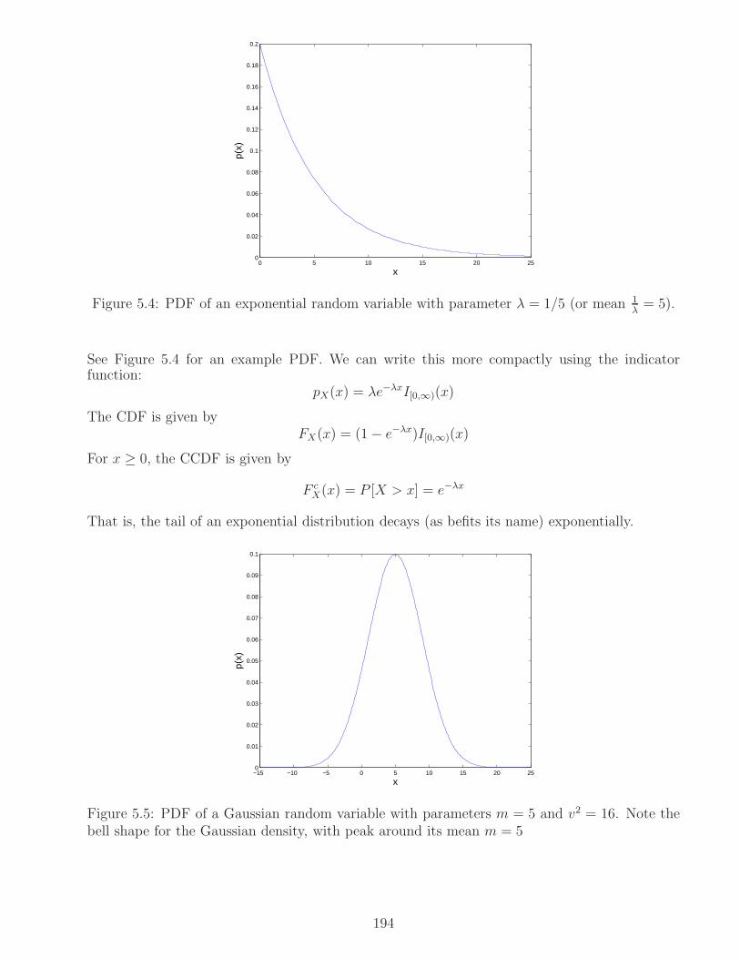
0 5 10 15 20 250

0.02

0.04

0.06

0.08

0.1

0.12

0.14

0.16

0.18

0.2

x

p(x)

Figure 5.4: PDF of an exponential random variable with parameter λ = 1/5 (or mean 1λ= 5).

See Figure 5.4 for an example PDF. We can write this more compactly using the indicatorfunction:

pX(x) = λe−λxI[0,∞)(x)

The CDF is given byFX(x) = (1− e−λx)I[0,∞)(x)

For x ≥ 0, the CCDF is given by

F cX(x) = P [X > x] = e−λx

That is, the tail of an exponential distribution decays (as befits its name) exponentially.

−15 −10 −5 0 5 10 15 20 250

0.01

0.02

0.03

0.04

0.05

0.06

0.07

0.08

0.09

0.1

x

p(x)

Figure 5.5: PDF of a Gaussian random variable with parameters m = 5 and v2 = 16. Note thebell shape for the Gaussian density, with peak around its mean m = 5

194

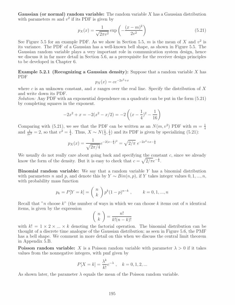
Gaussian (or normal) random variable: The random variable X has a Gaussian distributionwith parameters m and v2 if its PDF is given by

pX(x) =1√2πv2

exp

(

−(x−m)2

2v2

)

(5.21)

See Figure 5.5 for an example PDF. As we show in Section 5.5, m is the mean of X and v2 isits variance. The PDF of a Gaussian has a well-known bell shape, as shown in Figure 5.5. TheGaussian random variable plays a very important role in communication system design, hencewe discuss it in far more detail in Section 5.6, as a prerequisite for the receiver design principlesto be developed in Chapter 6.

Example 5.2.1 (Recognizing a Gaussian density): Suppose that a random variable X hasPDF

pX(x) = ce−2x2+x

where c is an unknown constant, and x ranges over the real line. Specify the distribution of Xand write down its PDF.Solution: Any PDF with an exponential dependence on a quadratic can be put in the form (5.21)by completing squares in the exponent.

−2x2 + x = −2(x2 − x/2) = −2

(

(x− 1

4)2 − 1

16

)

Comparing with (5.21), we see that the PDF can be written as an N(m, v2) PDF with m = 14

and 12v2

= 2, so that v2 = 14. Thus, X ∼ N(1

4, 14) and its PDF is given by specializing (5.21):

pX(x) =1

√

2π/4e−2(x− 1

4)2 =

√

2/π e−2x2+x− 18

We usually do not really care about going back and specifying the constant c, since we alreadyknow the form of the density. But it is easy to check that c =

√

2/πe−18 .

Binomial random variable: We say that a random variable Y has a binomial distributionwith parameters n and p, and denote this by Y ∼ Bin(n, p), if Y takes integer values 0, 1, ..., n,with probability mass function

pk = P [Y = k] =

(

nk

)

pk(1− p)n−k , k = 0, 1, ..., n

Recall that ”n choose k” (the number of ways in which we can choose k items out of n identicalitems, is given by the expression

(

nk

)

=n!

k!(n− k)!

with k! = 1 × 2 × ... × k denoting the factorial operation. The binomial distribution can bethought of a discrete time analogue of the Gaussian distribution; as seen in Figure 5.6, the PMFhas a bell shape. We comment in more detail on this when we discuss the central limit theoremin Appendix 5.B.

Poisson random variable: X is a Poisson random variable with parameter λ > 0 if it takesvalues from the nonnegative integers, with pmf given by

P [X = k] =λk

k!e−λ , k = 0, 1, 2, ...

As shown later, the parameter λ equals the mean of the Poisson random variable.

195

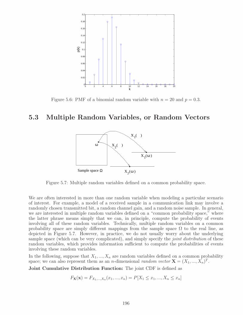
0 2 4 6 8 10 12 14 16 18 200

0.02

0.04

0.06

0.08

0.1

0.12

0.14

0.16

0.18

0.2

k

p(k)

Figure 5.6: PMF of a binomial random variable with n = 20 and p = 0.3.

5.3 Multiple Random Variables, or Random Vectors

ω

1 ω

2X ( )ω

X ( )1

2X ( )

ΩSample space

X ( )

Figure 5.7: Multiple random variables defined on a common probability space.

We are often interested in more than one random variable when modeling a particular scenarioof interest. For example, a model of a received sample in a communication link may involve arandomly chosen transmitted bit, a random channel gain, and a random noise sample. In general,we are interested in multiple random variables defined on a “common probability space,” wherethe latter phrase means simply that we can, in principle, compute the probability of eventsinvolving all of these random variables. Technically, multiple random variables on a commonprobability space are simply different mappings from the sample space Ω to the real line, asdepicted in Figure 5.7. However, in practice, we do not usually worry about the underlyingsample space (which can be very complicated), and simply specify the joint distribution of theserandom variables, which provides information sufficient to compute the probabilities of eventsinvolving these random variables.

In the following, suppose that X1, ..., Xn are random variables defined on a common probabilityspace; we can also represent them as an n-dimensional random vector X = (X1, ..., Xn)

T .

Joint Cumulative Distribution Function: The joint CDF is defined as

FX(x) = FX1,...,Xn(x1, ..., xn) = P [X1 ≤ x1, ..., Xn ≤ xn]

196

Joint Probability Density Function: When the joint CDF is continuous, we can define thejoint PDF as follows:

pX(x) = pX1,...,Xn(x1, ..., xn) =∂

∂x1...

∂

∂xnFX1,...,Xn(x1, ..., xn)

We can recover the joint CDF from the joint PDF by integrating:

FX(x) = FX1,...,Xn(x1, ..., xn) =

∫ x1

−∞...

∫ xn

−∞pX1,...,Xn(u1, ..., un)du1...dun

The joint PDF must be nonnegative and must integrate to one over n-dimensional space. Theprobability of a particular subset of n-dimensional space is obtained by integrating the joint PDFover the subset.

Joint Probability Mass Function (PMF): For discrete random variables, the joint PMF isdefined as

pX(x) = pX1,...,Xn(x1, ..., xn) = P [X1 = x1, ..., Xn = xn]

Marginal distributions: The marginal distribution for a given random variable (or set ofrandom variables) can be obtained by integrating or summing over all possible values of therandom variables that we are not interested in. For CDFs, this simply corresponds to settingthe appropriate arguments in the joint CDF to infinity. For example,

FX(x) = P [X ≤ x] = P [X ≤ x, Y ≤ ∞] = FX,Y (x,∞)

For continuous random variables, the marginal PDF is obtained from the joint PDF by “inte-grating out” the undesired random variable:

pX(x) =

∫ ∞

−∞pX,Y (x, y)dy , −∞ < x <∞

For discrete random variables, we sum over the possible values of the undesired random variable:

pX(x) =∑

y∈ Y

pX,Y (x, y) , x∈X

where X and Y denote the set of possible values taken by X and Y , respectively.

Example 5.3.1 (Joint and marginal densities): Random variables X and Y have jointdensity given by

pX,Y (x, y) =

c xy, 0 ≤ x, y ≤ 12c xy, −1 ≤ x, y ≤ 00, else

where the constant c is not specified.(a) Find the value of c.(b) Find P [X + Y < 1].(c) Specify the marginal distribution of X .Solution:(a) We find the constant using the observation that the joint density must integrate to one:

1 =∫ ∫

pX,Y (x, y) dx dy

= c∫ 1

0

∫ 1

0xy dx dy + 2c

∫ 0

−1

∫ 0

−1xy dx dy

= c x2

2

∣

∣

∣

1

0

y2

2

∣

∣

∣

1

0+ 2c x2

2

∣

∣

∣

0

−1

y2

2

∣

∣

∣

0

−1= 3c/4

197

0

x+y=1

Density =cxy

Density =

2cxy

x

y

1

−1

−1

0 1

Integrate density over shaded area

to find P[X+Y < 1]

1

1

Figure 5.8: Joint density in Example 5.3.1.

Thus, c = 4/3.(b) The required probability is obtained by integrating the joint density over the shaded area inFigure 5.8. We obtain

P [X + Y < 1] =∫ 1

y=0

∫ 1−y

x=0cxydxdy +

∫ 0

y=−1

∫ 0

x=−12cdxdy

= c∫ 1

y=0

(

x2

2

∣

∣

∣

1−y

0

)

ydy + 2cx2

2

∣

∣

∣

0

−1

y2

2

∣

∣

∣

0

−1

= c∫ 1

y=0y (1−y)2

2dy + 2c/4 = c/24 + c/2 = 13c/24

= 13/18

We could have computed this probability more quickly in this example by integrating the jointdensity over the unshaded area to find P [X + Y ≥ 1], since this area has a simpler shape:

P [X + Y ≥ 1] =∫ 1

y=0

∫ 1

x=1−ycxydxdy = c

∫ 1

y=0

(

x2

2

∣

∣

∣

1

1−y

)

ydy

= (c/2)∫ 1

y=0y(2y − y2)dy = 5c/24 = 5/18

from which we get that P [X + Y < 1] = 1− P [X + Y ≥ 1] = 13/18.(c) The marginal density of X is found by integrating the joint density over all possible valuesof Y . For 0 ≤ x ≤ 1, we obtain

pX(x) =

∫ 1

0

c xy dy = c xy2

2

∣

∣

∣

1

y=0= c x/2 = 2x/3 (5.22)

For −1 ≤ x ≤ 0, we have

pX(x) =

∫ 1

0

2c xy dy = 2c xy2

2

∣

∣

∣

1

y=0= −c x = −4x/3 (5.23)

Conditional density: The conditional density of Y given X is defined as

pY |X(y|x) =pX,Y (x, y)

pX(x)(5.24)

where the definition applies for both PDFs and PMFs, and where we are interested in values ofx such that pX(x) > 0. For jointly continuous X and Y , the conditional density p(y|x) has theinterpretation

pY |X(y|x)∆y ≈ P[

Y ∈ [y, y +∆y]∣

∣X ∈ [x, x+∆x]]

(5.25)

198

for ∆x, ∆y small. For discrete random variables, the conditional pmf is simply the followingconditional probability:

pY |X(y|x) = P [Y = y|X = x] (5.26)

Example 5.3.2 Continuing with Example 5.3.1, let us find the conditional density of Y givenX . For X = x∈ [0, 1], we have pX,Y (x, y) = c xy, with 0 ≤ y ≤ 1 (the joint density is zero forother values of y, under this conditioning on X). Applying (5.24), and substituting (5.22), weobtain


pX(x)=

cxy

cx/2= 2y , 0 ≤ y ≤ 1 (for 0 ≤ x ≤ 1)

Similarly, for X = x∈ [−1, 0], we obtain, using (5.23), that


pX(x)=

2cxy

−cx = −2y , − 1 ≤ y ≤ 0 (for − 1 ≤ x ≤ 0)

We can now compute conditional probabilities using the preceding conditional densities. Forexample,

P [Y < −0.5|X = −0.5] =

∫ −0.5

−1

(−2y)dy = −y2∣

∣

∣

−0.5

−1= 3/4

whereas P [Y < 0.5|X = −0.5] = 1 (why?).

Bayes’ rule for conditional densities: Given the conditional density of Y given X , theconditional density for X given Y is given by

pX|Y (x|y) = pY |X(y|x)pX(x)

pY (y)=

pY |X(y|x)pX(x)∫pY |X(y|x)pX(x)dx

, continuous random variables

pX|Y (x|y) = pY |X(y|x)pX(x)

pY (y)=

pY |X(y|x)pX(x)∑

x pY |X(y|x)pX(x), discrete random variables

We can also mix discrete and continuous random variables in applying Bayes’ rule, as illustratedin the following example.

Example 5.3.3 (Conditional probability and Bayes’ rule with discrete and continuousrandom variables) A bit sent by a transmitter is modeled as a random variable X taking values0 and 1 with equal probability. The corresponding observation at the receiver is modeled by areal-valued random variable Y . The conditional distribution of Y given X = 0 is N(0, 4). Theconditional distribution of Y given X = 1 is N(10, 4). This might happen, for example, withon-off signaling, where we send a signal to send 1, and send nothing when we want to send 0.The receiver therefore sees signal plus noise if 1 is sent, and sees only noise if 0 is sent, and theobservation Y , presumably obtained by processing the received signal, has zero mean if 0 is sent,and nonzero mean if 1 is sent.(a) Write down the conditional densities of Y given X = 0 and X = 1, respectively.(b) Find P [Y = 7|X = 0], P [Y = 7|X = 1] and P [Y = 7].(c) Find P [Y ≥ 7|X = 0].(d) Find P [Y ≥ 7|X = 1].(e) Find P [X = 0|Y = 7].Solution to (a): We simply plug in numbers into the expression (5.21) for the Gaussian densityto obtain:

p(y|x = 0) =1√8πe−y2/8 , p(y|x = 1)dy =

1√8πe−(y−10)2/8

199

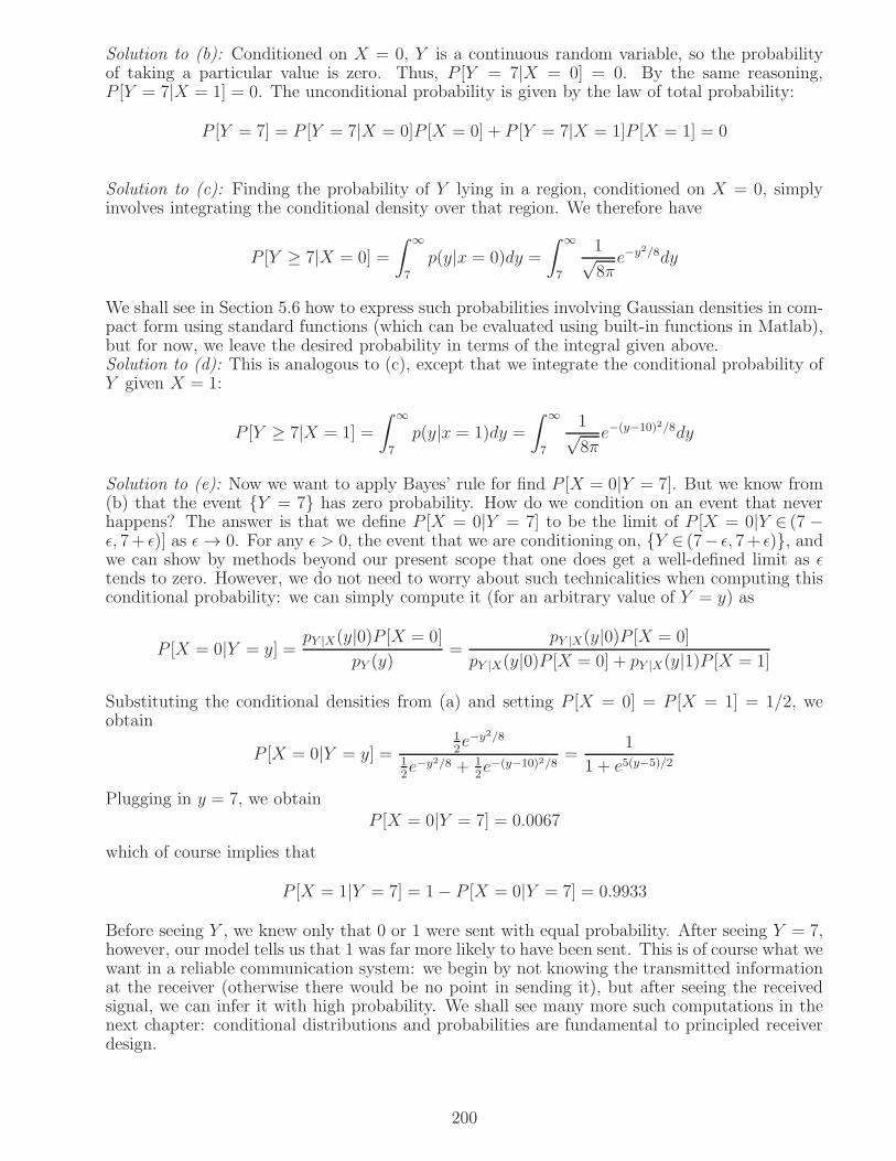
Solution to (b): Conditioned on X = 0, Y is a continuous random variable, so the probabilityof taking a particular value is zero. Thus, P [Y = 7|X = 0] = 0. By the same reasoning,P [Y = 7|X = 1] = 0. The unconditional probability is given by the law of total probability:

P [Y = 7] = P [Y = 7|X = 0]P [X = 0] + P [Y = 7|X = 1]P [X = 1] = 0

Solution to (c): Finding the probability of Y lying in a region, conditioned on X = 0, simplyinvolves integrating the conditional density over that region. We therefore have

P [Y ≥ 7|X = 0] =

∫ ∞

7

p(y|x = 0)dy =

∫ ∞

7

1√8πe−y2/8dy

We shall see in Section 5.6 how to express such probabilities involving Gaussian densities in com-pact form using standard functions (which can be evaluated using built-in functions in Matlab),but for now, we leave the desired probability in terms of the integral given above.Solution to (d): This is analogous to (c), except that we integrate the conditional probability ofY given X = 1:

P [Y ≥ 7|X = 1] =

∫ ∞

7

p(y|x = 1)dy =

∫ ∞

7

1√8πe−(y−10)2/8dy

Solution to (e): Now we want to apply Bayes’ rule for find P [X = 0|Y = 7]. But we know from(b) that the event Y = 7 has zero probability. How do we condition on an event that neverhappens? The answer is that we define P [X = 0|Y = 7] to be the limit of P [X = 0|Y ∈ (7 −ǫ, 7+ ǫ)] as ǫ→ 0. For any ǫ > 0, the event that we are conditioning on, Y ∈ (7− ǫ, 7+ ǫ), andwe can show by methods beyond our present scope that one does get a well-defined limit as ǫtends to zero. However, we do not need to worry about such technicalities when computing thisconditional probability: we can simply compute it (for an arbitrary value of Y = y) as

P [X = 0|Y = y] =pY |X(y|0)P [X = 0]

pY (y)=

pY |X(y|0)P [X = 0]

pY |X(y|0)P [X = 0] + pY |X(y|1)P [X = 1]

Substituting the conditional densities from (a) and setting P [X = 0] = P [X = 1] = 1/2, weobtain

P [X = 0|Y = y] =12e−y2/8

12e−y2/8 + 1

2e−(y−10)2/8

=1

1 + e5(y−5)/2

Plugging in y = 7, we obtainP [X = 0|Y = 7] = 0.0067

which of course implies that

P [X = 1|Y = 7] = 1− P [X = 0|Y = 7] = 0.9933

Before seeing Y , we knew only that 0 or 1 were sent with equal probability. After seeing Y = 7,however, our model tells us that 1 was far more likely to have been sent. This is of course what wewant in a reliable communication system: we begin by not knowing the transmitted informationat the receiver (otherwise there would be no point in sending it), but after seeing the receivedsignal, we can infer it with high probability. We shall see many more such computations in thenext chapter: conditional distributions and probabilities are fundamental to principled receiverdesign.

200

Independent Random Variables: Random variables X1, ..., Xn are independent if

P [X1 ∈A1, ..., Xn ∈An] = P [X1 ∈A1]...P [Xn ∈An]

for any subsets A1, ..., An. That is, events defined in terms of values taken by these random vari-ables are independent of each other. This implies, for example, that the conditional probabilityof an event defined in terms of one of these random variables, conditioned on events defined interms of the other random variables, equals the unconditional probability:

P [X1∈A1|X2 ∈A2, ..., Xn ∈An] = P [X1∈A1]

In terms of distributions and densities, independence means that joint distributions are productsof marginal distributions, and joint densities are products of marginal densities.

Joint distribution is product of marginals for independent random variables: IfX1, ..., Xn are independent, then their joint CDF is a product of the marginal CDFs:

FX1,...,Xn(x1, ..., xn) = FX1(x1)...FXn(xn)

and their joint density (PDF or PMF) is a product of the marginal densities:

pX1,...,Xn(x1, ..., xn) = pX1(x1)...pXn(xn)

Independent and identically distributed (i.i.d.) random variables: We are often inter-ested in collections of independent random variables in which each random variable has the samemarginal distribution. We call such random variables independent and identically distributed.

Example 5.3.4 (A sum of i.i.d. Bernoulli random variables is a Binomial random variable):Let X1, ..., Xn denote i.i.d. Bernoulli random variables with P [X1 = 1] = 1−P [X1 = 0] = p, andlet Y = X1+...+Xn denote their sum. We could think ofXi denoting whether the ith coin flip (ofa possibly biased coin, if p 6= 1

2) yield heads, where successive flips have independent outcomes,

so that Y is the number of heads obtained in n flips. For communications applications, Xi coulddenote whether the ith bit in a sequence of n bits is incorrectly received, with successive biterrors modeled as independent, so that Y is the total number of bit errors. The random variableY takes discrete values in 0, 1, ..., n. Its PMF is given by

P [Y = k] =

(

nk

)

pk(1− p)n−k , k = 0, 1, ..., n

That is, Y ∼ Bin(n, p). To see why, note that Y = k requires that exactly k of the Xi takevalue 1, with the remaining n − k taking value 0. Let us compute the probability of one suchoutcome, X1 = 1, ..., Xk = 1, Xk+1 = 0, ..., Xn = 0:P [X1 = 1, ..., Xk = 1, Xk+1 = 0, ..., Xn = 0] = P [X1 = 1]...P [Xk = 1]P [Xk+1 = 0]...P [Xn = 0]

= pk(1− p)n−k

Clearly, any other outcome with exactly k ones has the same probability, given the i.i.d. natureof the Xi. We can now sum over the probabilities of these mutually exclusive events, notingthat there are exactly “n choose k” such outcomes (the number of ways in which we can choosethe k random variables Xi which take the value one) to obtain the desired PMF.

Density of sum of independent random variables: Suppose that X1 and X2 are indepen-dent continuous random variables, and let Y = X1 +X2. Then the PDF of Y is a convolutionof the PDFs of X1 and X2:

pY (y) = (pX1 ∗ pX2)(y) =

∫ ∞

−∞pX1(x1)pX2(y − x1) dx1

For discrete random variables, the same result holds, except that the PMF is given by a discrete-time convolution of the PMFs of X1 and X2.

201

=

Density of X2Density of X1 Dsnsity of Y = X + X21

0 1

1

1/2

−11−1 0 1 2

1/2

*

Figure 5.9: The sum of two independent uniform random variables has a PDF with trapezoidalshape, obtained by convolving two boxcar-shaped PDFs.

Example 5.3.5 (Sum of two uniform random variables) Suppose that X1 is uniformlydistributed over [0, 1], and X2 is uniformly distributed over [−1, 1]. Then Y = X1 + X2 takesvalues in the interval [−1, 2], and its density is the convolution shown in Figure 5.9.

Of particular interest to us are jointly Gaussian random variables, which we discuss in moredetail in Section 5.6.

Notational simplification: In the preceding definitions, we have distinguished between differ-ent random variables by using subscripts. For example, the joint density of X and Y is denotedby pX,Y (x, y), where X , Y denote the random variables, and x, y, are dummy variables that wemight, for example, integrate over when evaluating a probability. We could easily use some othernotation for the dummy variables, e.g., the joint density could be denoted as pX,Y (u, v). Afterall, we know that we are talking about the joint density of X and Y because of the subscripts.However, carrying around the subscripts is cumbersome. Therefore, from now on, when thereis no scope for confusion, we drop the subscripts and use the dummy variables to also denotethe random variables we are talking about. For example, we now use p(x, y) as shorthand forpX,Y (x, y), choosing the dummy variables to be lower case versions of the random variables theyare associated with. Similarly, we use p(x) to denote the density of X , p(y) to denote the densityof Y , and p(y|x) to denote the conditional density of Y given X . Of course, we revert to thesubscript-based notation whenever there is any possibility of confusion.

5.4 Functions of random variables

Y( )

ω

ω

ωX( )ωg(X( ))ΩSample space

X( ) g( )

Y( )=

Figure 5.10: A function of a random variable is also a random variable.

We review here methods of determining the distribution of functions of random variables. IfX = X(ω) is a random variable, so is Y (ω) = g(X(ω)), since it is a mapping from the samplespace to the real line which is a composition of the original mapping X and the function g, asshown in Figure 5.10.

Method 1 (find the CDF first): We proceed from definition to find the CDF of Y = g(X)as follows:

FY (y) = P [Y ≤ y] = P [g(X) ≤ y] = P [X ∈A(y)]

202

where A(y) = x : g(x) ≤ y. We can now use the CDF or density of X to evaluate the extremeright-hand side. Once we find the CDF of Y , we can find the PMF or PDF as usual.

to Y <= y

yy

y = x2

y

−

x

x

p(x)

Range of X corresponding

Figure 5.11: Finding the CDF of Y = X2.

Example 5.4.1 (Application of Method 1) Suppose that X is a Laplacian random variablewith density

pX(x) =1

2e−|x|

Find the CDF and PDF of Y = X2.In method 1, we find the CDF of Y first, and then differentiate to find the PDF. First, note thatY takes only nonnegative values, so that FY (y) = 0 for y < 0. For y ≥ 0, we have

FY (y) = P [Y ≤ y] = P [X2 ≤ y] = P [−√y ≤ X ≤ √

y]

=∫

√y

−√ypX(x)dx =

∫

√y

−√y

12e−|x|dx =

∫

√y

0e−xdx

= 1− e−√y , y ≥ 0

We can now differentiate the CDF to obtain the PDF of Y :

pY (y) =d

dyFY (y) =

e−√y

2√y, y ≥ 0

(The CDF and PDF are zero for y < 0, since Y only takes nonnegative values.)

203

Method 2 (find the PDF directly): For differentiable g(x) and continuous random variables,we can compute the PDF directly. Suppose that g(x) = y is satisfied for x = x1, ..., xm. Wecan then express xi as a function of y: xi = hi(y) For g(x) = x2, this corresponds to x1 =

√y

and x2 = −√y. The probability of X lying in a small interval [xi, xi + ∆x] is approximately

pX(xi)∆x, where we take the increment ∆x > 0. For smooth g, this corresponds to Y lying in asmall interval around y, where we need to sum up the probabilities corresponding to all possiblevalues of x that get us near the desired value of y. We therefore get

pY (y)|∆y| =m∑

i=1

pX(xi)∆x

where we take the magnitude of the Y increment ∆y because a positive increment in x can causea positive or negative increment in g(x), depending on the slope at that point. We thereforeobtain

pY (y) =

m∑

i=1

pX(xi)

|dy/dx|∣

∣

∣

xi=hi(y)(5.27)

We now redo Example 5.4.1 using Method 2.

Example 5.4.2 (application of Method 2) For the setting of Example 5.4.1, we wish to findthe PDF using Method 2. For y = g(x) = x2, we have x = ±√

y (we only consider y ≥ 0, sincethe PDF is zero for y < 0), with derivative dy/dx = 2x. We can now apply (5.27) to obtain:

pY (y) =pX(

√y)

|2√y| +pX(−

√y)

| − 2√y| =

e−√y

2√y, y ≥ 0

as before.

Since Method 1 starts from the definition of CDF, it generalizes to multiple random variables(i.e., random vectors) in a straightforward manner, at least in principle. For example, supposethat Y1 = g1(X1, X2) and Y2 = g2(X1, X2). Then the joint CDF of Y1 and Y2 is given by

FY1,Y2(y1, y2) = P [Y1 ≤ y1, Y2 ≤ y2] = P [g1(X1, X2) ≤ y1, g2(X1, X2) ≤ y2] = P [(X1, X2)∈A(y1, y2)]

where A(y1, y2) = (x1, x2) : g1(x1, x2) ≤ y1, g2(x1, x2) ≤ y2. In principle, we can now use thejoint distribution to compute the preceding probability for each possible value of (y1, y2). Ingeneral, Method 1 works for Y = g(X), where Y is an n-dimensional random vector which isa function of an m-dimensional random vector X (in the preceding, we considered m = n =2). However, evaluating probabilities involving m-dimensional random vectors can get prettycomplicated even for m = 2. A generalization of Method 2 is often preferred as a way of directlyobtaining PDFs when the functions involved are smooth enough, and when m = n. We reviewthis next.

Method 2 for random vectors: Suppose that Y = (Y1, ..., Yn)T is an n × 1 random vector

which is a function of another n × 1 vector X = (X1, ..., Xn)T . That is, Y = g(X), or Yk =

gk(X1, ..., Xn), k = 1, .., n. As before, suppose that y = g(x) has m solutions, x1, ...,xm, with theith solution written in terms of y as xi = hi(y). The probability of Y lying in an infinitesimalvolume is now given by

pY(y) |dy| =m∑

i=1

pX(xi) |dx|

204

In order to relate the lengths of the vector increments |dy| and |dx|, it no longer suffices toconsider a scalar derivative. We now need the Jacobian matrix of partial derivatives of y = g(x)with respect to x, defined as:

J(y;x) =

∂y1∂x1

· · · ∂y1∂xn

......

∂yn∂x1

· · · ∂yn∂xn

(5.28)

The lengths of the vector increments are related as

|dy| = |det (J(y;x)) ||dx|

where det (M) denotes the determinant of a square matrix M. Thus, if y = g(x) hasm solutions,x1, ...,xm, with the ith solution written in terms of y as xi = hi(y), then the density at y isgiven by

pY(y) =

m∑

i=1

pX(xi)

|det(J(y;x))|∣

∣

∣

xi=hi(y)(5.29)

Depending on how the functional relationship between X and Y is specified, it might sometimesbe more convenient to find the Jacobian of x with respect to y:

J(x;y) =

∂x1

∂y1· · · ∂x1

∂yn...

...∂xn

∂y1· · · ∂xn

∂yn

(5.30)

We can use this in (5.29) by noting the two Jacobian matrices for a given pair of values (x,y)are inverses of each other:

J(x;y) = (J(y;x))−1

This implies that their determinants are reciprocals of each other:

det(J(x;y)) =1

det(J(y;x))

We can therefore rewrite (5.29) as follows:

pY(y) =

m∑

i=1

pX(xi) |det(J(x;y))|∣

∣

∣

xi=hi(y)(5.31)

Example 5.4.3 (Rectangular to Polar Transformation): For random variables X1, X2

with joint density pX1,X2, think of (X1, X2) as a point in two-dimensional space in Cartesiancoordinates. The corresponding polar coordinates are given by

R =√

X21 +X2

2 , Φ = tan−1X2

X1

(5.32)

(a) Find the general expression for joint density pR,Φ.(b) Specialize to a situation in which X1 and X2 are i.i.d. N(0, 1) random variables.Solution, part (a): Finding the Jacobian involves taking partial derivatives in (5.32). However,in this setting, taking the Jacobian the other way around, as in (5.30), is simpler:

x1 = r cosφ , x2 = r sinφ

205

so that

J(rect; polar) =

(

∂x1

∂r∂x1

∂φ∂x2

∂r∂x2

∂φ

)

=

(

cosφ −r sinφsin φ r cos φ

)

We see thatdet (J(rect; polar)) = r

(

cos2 φ+ sin2 φ)

= r

Noting that the rectangular-polar transformation is one-to-one, we have from (5.31) that

pR,Φ(r, φ) = pX1,X2(x1, x2)|det(J(rect; polar))|∣

∣

∣

x1=r cosφ,x2=r sinφ

= rpX1,X2(r cosφ, r sinφ) , r ≥ 0, 0 ≤ φ ≤ 2π(5.33)

Solution, part (b): For X1, X2 i.i.d. N(0, 1), we have

pX1,X2(x1, x2) = pX1(x1)pX2(x2) =1√2πe−x2

1/21√2πe−x2

2/2

Plugging into (5.33) and simplifying, we obtain

pR,Φ(r, φ) =r

2πe−r2/2 , r ≥ 0, 0 ≤ φ ≤ 2π

We can find the marginal densities of R and Φ by integrating out the other variable, but in thiscase, we can find them by inspection, since the joint density clearly decomposes into a product offunctions of r and φ alone. With appropriate normalization, each of these functions is a marginaldensity. We can now infer that R and Φ are independent, with

pR(r) = re−r2/2 , r ≥ 0

and

pΦ(φ) =1

2π, 0 ≤ φ ≤ 2π

The amplitude R in this case follows a Rayleigh distribution, while the phase Φ is uniformlydistributed over [0, 2π].

5.5 Expectation

We now discuss computation of statistical averages, which are often the performance measuresbased on which a system design is evaluated.

Expectation: The expectation, or statistical average, of a function of a random variable X isdefined as

E[g(X)] =∫

g(x)p(x)dx , continuous random variableE[g(X)] =

∑

g(x)p(x) , discrete random variable(5.34)

Note that the expectation of a deterministic constant, therefore, is simply the constant itself.

Expectation is a linear operator: We have

E [a1X1 + a2X2 + b] = a1E[X1] + a2E[X2] + b

where a1, a2, b, are any constants.

206

Mean: The mean of a random variable X is E[X ].

Variance: The variance of a random variable X is a measure of how much it fluctuates aroundits mean:

var(X) = E[

(X − E[X ])2]

(5.35)

Expanding out the square, we have

var(X) = E[

X2 − 2XE[X ] + (E[X ])2]

Using the linearity of expectation, we can simplify to obtain the following alternative formulafor variance:

var(X) = E[X2]− (E[X ])2 (5.36)

The square root of the variance is called the standard deviation.

Effect of Scaling and Translation: For Y = aX + b, it is left as an exercise to show that

E[Y ] = E[aX + b] = aE[X ] + bvar(Y ) = a2var(X)

(5.37)

Normalizing to zero mean and unit variance: We can specialize (5.37) to Y = X−E[X]√var(X)

, to

see that E[Y ] = 0 and var(Y ) = 1.

Example 5.5.1 (PDF after scaling and translation): If X has density pX(x), then Y =(X − a)/b has density

pY (y) = |b|pX(by + a) (5.38)

This follows from a straightforward application of Method 2 in Section 5.4. Specializing to aGaussian random variable X ∼ N(m, v2) with mean m and variance v2 (we review mean andvariance later), consider a normalized version Y = (X −m)/v. Applying (5.38) to the Gaussiandensity, we obtain:

pY (y) =1√2πe−

y2

2

which can be recognized as an N(0, 1) density. Thus, if X ∼ N(m, v2), then Y = X−mv

∼ N(0, 1)is a standard Gaussian random variable. This enables us to express probabilities involvingGaussian random variables compactly in terms of the CDF and CCDF of a standard Gaussianrandom variable, as we see later when we deal extensively with Gaussian random variables whenmodeling digital communication systems.

Moments: The nth moment of a random variable X is defined as E[Xn]. From (5.36), we seethat specifying the mean and variance is equivalent to specifying the first and second moments.Indeed, it is worth rewriting (5.36) as an explicit reminder that the second moment is the sumof the mean and variance:

E[X2] = (E[X ])2 + var(X) (5.39)

Example 5.5.2 (Moments of an exponential random variable): Suppose that X ∼Exp(λ). We compute its mean using integration by parts, as follows:

E[X ] =∫∞0xλe−λx dx = −xe−λx

∣

∣

∣

∞

0+∫∞0

ddxxe−λxdx

=∫∞0e−λxdx = e−λx

−λ

∣

∣

∣

∞

0

= 1λ

(5.40)

207

Similarly, using integration by parts twice, we can show that

E[X2] =2

λ2

Using (5.36), we obtain

var(X) = E[X2]− (E[X ])2 =1

λ2(5.41)

In general, we can use repeated integration by parts to evaluate higher moments of the exponentialrandom variable to obtain

E[Xn] =

∫ ∞

0

xnλe−λx dx =n!

λn, n = 1, 2, 3, ...

(A proof of the preceding formula using mathematical induction is left as an exercise.)

As a natural follow-up to the computations in the preceding example, let us introduce the gammafunction, which is useful for evaluating integrals associated with expectation computations forseveral important random variables.

Gamma function: The Gamma function, Γ(x), is defined as

Γ(x) =

∫ ∞

0

tx−1e−tdt , x > 0

In general, integration by parts can be used to show that

Γ(x+ 1) = xΓ(x) , x > 0 (5.42)

Noting that Γ(1) = 1, we can now use induction to specify the Gamma function for integerarguments.

Γ(n) = (n− 1)! , n = 1, 2, 3, ... (5.43)

This is exactly the same computation as we did in Example 5.5.2: Γ(n) equals the the (n− 1)thmoment of an exponential random variable with λ = 1 (and hence mean 1

λ= 1).

The Gamma function can also be computed for non-integer arguments. Just an integer argumentsof the Gamma function are useful for exponential random variables, ”integer-plus-half” argumentsare useful for evaluating the moments of Gaussian random variables. We can evaluate these using(5.42) given the value of the gamma function at x = 1/2.

Γ (1/2) =

∫ ∞

0

t−12 e−t dt =

√π (5.44)

For example, we can infer that

Γ (5/2) = (3/2)(1/2)Γ (1/2) =3

4

√π

Example 5.5.3 (Mean and variance of a Gaussian random variable): We now show thatX ∼ N(m, v2) has mean m and variance v2. The mean of X is given by the following expression:

E[X ] =

∫ ∞

−∞x

1√2πv2

e−(x−m)2

2v2 dx

208

Let us first consider the change of variables t = (x−m)/v, so that dx = v dt. Then

E[X ] =

∫ ∞

−∞(tv +m)

1√2πv2

e−t2/2v dt

Note that te−t2/2 is an odd function, and therefore integrates out to zero over the real line. Wetherefore obtain

E[X ] =

∫ ∞

−∞m

1√2πv2

e−t2/2v dt = m

∫ ∞

−∞

1√2πe−t2/2 dt = m

recognizing that the integral on the extreme right-hand side is the N(0, 1) PDF, which mustintegrate to one. The variance is given by

var(X) = E[(X −m)2] =

∫ ∞

−∞(x−m)2

1√2πv2

e−(x−m)2

2v2 dx

With a change of variables t = (x−m)/v as before, we obtain

var(X) = v2∫ ∞

−∞t2

1√2πe−t2/2 dt = 2v2

∫ ∞

0

t21√2πe−t2/2 dt

since the integrand is an even function of t. Substituting z = t2/2, so that dz = tdt =√2zdt,

we obtainvar(X) = 2v2

∫∞0

2z 1√2πe−z dz√

2z= 2v2 1√

π

∫∞0z1/2e−z

= 2v2 1√πΓ(3/2) = v2

since Γ(3/2) = (1/2)Γ(1/2) =√π/2.

The change of variables in the computations in the preceding example is actually equivalentto transforming the N(m, v2) random variable that we started with to a standard GaussianN(0, 1) random variable as in Example 5.5.1. As we mentioned earlier (this is important enoughto be worth repeating), when we handle Gaussian random variables more extensively in laterchapters, we prefer making the transformation up front when computing probabilities, ratherthan changing variables inside integrals.

As a final example, we show that the mean of a Poisson random variable with parameter λ isequal to λ.

Example 5.5.4 (Mean of a Poisson random variable): The mean is given by

E[X ] =

∞∑

k=0

kP [X = k] =

∞∑

k=1

kλk

k!e−λ

where we have dropped the k = 0 term from the extreme right hand side, since it does notcontribute to the mean. Noting that k

k!= 1

(k−1)!, we have

E[X ] =

∞∑

k=1

λk

(k − 1)!e−λ = λe−λ

∞∑

k=1

λk−1

(k − 1)!= λ

since ∞∑

k=1

λk−1

(k − 1)!=

∞∑

l=0

λl

l!= eλ

where we set l = k−1 to get an easily recognized form for the series expansion of an exponential.

209

5.5.1 Expectation for random vectors

So far, we have talked about expectations involving a single random variable. Expectationswith multiple random variables are defined in exactly the same way: as in (5.34), replacing thescalar random variable and the corresponding dummy variable for summation or integration bya vector.

E[g(X)] = E[g(X1, ..., Xn)] =∫

g(x)p(x) dx , jointly continuous random variables=∫∞x1=−∞ ...

∫∞xn=−∞ g(x1, ..., xn)p(x1, ..., xn) dx1...dxn

E[g(X)] = E[g(X1, ..., Xn)] =∑

x g(x)p(x) , discrete random variables=∑

x1...∑

xng(x1, ..., xn)p(x1, ..., xn)

(5.45)

Product of expectations for independent random variables: When the random variablesinvolved are independent, and the function whose expectation is to be evaluated decomposesinto a product of functions of each individual random variable, then the preceding computationinvolves a product of expectations, each involving only one random variable:

E[g1(X1)...gn(Xn)] = E[g1(X1)]...E[gn(Xn)] , X1, ..., Xn independent (5.46)

Example 5.5.5 (Computing an expectation involving independent random variables):Suppose that X1 ∼ N(1, 1) and X2 ∼ N(−3, 4) are independent. Find E[(X1 +X2)

2].Solution: We have

E[(X1 +X2)2] = E[X2

1 +X22 + 2X1X2]

We can now use linearity to compute the expectations of each of the three terms on the right-hand side separately. We obtain E[X2

1 ] = (E[X1])2 + var(X1) = 12 + 1 = 2, E[X2

2 ] = (E[X2])2 +

var(X2) = (−3)2 + 4 = 13, and E[2X1X2] = 2E[X1]E[X2] = 2(1)(−3) = −6, so that

E[(X1 +X2)2] = 2 + 13− 6 = 9

Variance is a measure of how a random variable fluctuates around its means. Covariance, definednext, is a measure of how the fluctuations of two random variables around their means arecorrelated.

Covariance: The covariance of X1 and X2 is defined as

cov(X1, X2) = E [(X1 − E[X1]) (X2 − E[X2])] (5.47)

As with variance, we can also obtain the following alternative formula:

cov(X1, X2) = E[X1X2]− E[X1]E[X2] (5.48)

Variance is the covariance of a random variable with itself: It is immediate from thedefinition that

var(X) = cov(X,X)

Uncorrelated random variables: Random variables X1 and X2 are said to be uncorrelatedif cov(X1, X2) = 0.

Independent random variables are uncorrelated: If X1 and X2 are independent, then theyare uncorrelated.This is easy to see from (5.48), since E[X1X2] = E[X1]E[X2] using (5.46).

210

Uncorrelated random variables need not be independent: Consider X ∼ N(0, 1) andY = X2. We see that that E[XY ] = E[X3] = 0 by the symmetry of the N(0, 1) density aroundthe origin, so that

cov(X, Y ) = E[XY ]− E[X ]E[Y ] = 0

Clearly, X and Y are not independent, since knowing the value of X determines the value of Y .

As we discuss in the next section, uncorrelated jointly Gaussian random variables are indeedindependent. The joint distribution of such random variables is determined by means and co-variances, hence we also postpone more detailed discussion of covariance computation until ourstudy of joint Gaussianity.

5.6 Gaussian Random Variables

We begin by repeating the definition of a Gaussian random variable.

Gaussian random variable: The random variable X is said to follow a Gaussian, or normaldistribution if its density is of the form:

p(x) =1√2πv2

exp

(

−(x−m)2

2v2

)

, −∞ < x <∞ (5.49)

where m = E[X ] is the mean of X , and v2 = var(X) is the variance of X . The Gaussian densityis therefore completely characterized by its mean and variance.Notation for Gaussian distribution: We use N(m, v2) to denote a Gaussian distributionwith mean m and variance v2, and use the shorthand X ∼ N(m, v2) to denote that a randomvariable X follows this distribution.

We have already noted the characteristic bell shape of the Gaussian PDF in the example plottedin Figure 5.5: the bell is centered around the mean, and its width is determined by the variance.We now develop a detailed framework for efficient computations involving Gaussian randomvariables.

Standard Gaussian random variable: A zero mean, unit variance Gaussian random variable,X ∼ N(0, 1), is termed a standard Gaussian random variable.

An important property of Gaussian random variables is that they remain Gaussian under scalingand translation. Suppose that X ∼ N(m, v2). Define Y = aX + b, where a, b are constants(assume a 6= 0 to avoid triviality). The density of Y can be found as follows:

p(y) =p(x)

| dydx|

∣

∣

∣

∣

∣

x=(y−b)/a

Noting that dydx

= a, and plugging in (5.49), we obtain

p(y) = 1|a|

1√2πv2

exp(

− ((y − b)/a−m)2 /(2v2))

= 1√2πa2v2

exp(

− (y − (am+ b))2 /(2a2v2))

Comparing with (5.49), we can see that Y is also Gaussian, with mean mY = am+b and variancev2Y = a2v2. This is important enough to summarize and restate.

Gaussianity is preserved under scaling and translationIf X ∼ N(m, v2), then Y = aX + b ∼ N(am+ b, a2v2).

211

As a consequence of the preceding result, any Gaussian random variable can be scaled andtranslated to obtain a “standard” Gaussian random variable with zero mean and unit variance.For X ∼ N(m, v2), Y = aX + b ∼ N(0, 1) if am+ b = 0 and a2v2 = 1 to have a = v, b = −vm.That is, Y = (X −m)/v ∼ N(0, 1).

Standard Gaussian random variableA standard Gaussian random variable N(0, 1) has mean zero and variance one.

Conversion of a Gaussian random variable into standard formIf X ∼ N(m, v2), then X−m

v∼ N(0, 1).

As the following example illustrates, this enables us to express probabilities involving any Gaus-sian random variable as probabilities involving a standard Gaussian random variable.

Example 5.6.1 Suppose that X ∼ N(5, 9). Then (X − 5)/√9 = (X − 5)/3 ∼ N(0, 1). Any

probability involving X can now be expressed as a probability involving a standard Gaussianrandom variable. For example,

P [X > 11] = P [(X − 5)/3 > (11− 5)/3] = P [N(0, 1) > 2]

We therefore set aside special notation for the cumulative distribution function (CDF) Φ(x) andcomplementary cumulative distribution function (CCDF) Q(x) of a standard Gaussian randomvariable. By virtue of the standard form conversion, we can now express probabilities involvingany Gaussian random variable in terms of the Φ or Q functions. The definitions of these functionsare illustrated in Figure 5.12, and the corresponding formulas are specified below.

x u

p(u)

Φ(x) Q(x)

Figure 5.12: The Φ and Q functions are obtained by integrating the N(0, 1) density over appro-priate intervals.

Φ(x) = P [N(0, 1) ≤ x] =

∫ x

−∞

1√2π

exp

(

−t2

2

)

dt (5.50)

Q(x) = P [N(0, 1) > x] =

∫ ∞

x

1√2π

exp

(

−t2

2

)

dt (5.51)

See Figure 5.13 for a plot of these functions. By definition, Φ(x)+Q(x) = 1. Furthermore, by thesymmetry of the Gaussian density around zero, Q(−x) = Φ(x). Combining these observations,we note that Q(−x) = 1 − Q(x), so that it suffices to consider only positive arguments for theQ function in order to compute probabilities of interest.

Let us now consider a few more Gaussian probability computations.

212

Q(x) Φ(x)

1

0 x

Figure 5.13: The Φ and Q functions.

Example 5.6.2 X is a Gaussian random variable with mean m = −5 and variance v2 = 4. Findexpressions in terms of the Q function with positive arguments for the following probabilities:P [X > 3], P [X < −8], P [X < −1], P [3 < X < 6], P [X2 − 2X > 15].Solution: We solve this problem by normalizing X to a standard Gaussian random variableX−m

v= X+5

2

P [X > 3] = P [X + 5

2>

3 + 5

2= 4] = Q(4)

P [X < −8] = P [X + 5

2<

−8 + 5

2= −1.5] = Φ(−1.5) = Q(1.5)

P [X < −1] = P [X + 5

2<

−1 + 5

2= 2] = Φ(2) = 1−Q(2)

P [3 < X < 6] = P [4 = 3+52< X+5

2< 6+5

2= 5.5]

= Φ(5.5)− Φ(4) = ((1−Q(5.5))− (1−Q(4))) = Q(4)−Q(5.5)

Computation of the probability that X2 − 2X > 15 requires that we express this event in termsof simpler events by factorization:

X2 − 2X − 15 = X2 − 5X + 3X − 15 = (X − 5)(X + 3)

This shows that X2 − 2X > 15, or X2 − 2X − 15 > 0, if and only if X − 5 > 0 and X + 3 > 0,or X − 5 < 0 and X + 3 < 0. The first event simplifies to X > 5, and the second to X < −3, sothat the desired probability is a union of two mutually exclusive events. We therefore have

P [X2 − 2X > 15] = P [X > 5] + P [X < −3] = Q(5+52) + Φ(−3+5

2)

= Q(5) + Φ(1) = Q(5) + 1−Q(1)

Interpreting the transformation to standard Gaussian: For X ∼ N(m, v2), the transfor-mation to standard Gaussian tells us that

P [X > m+ αv] = P

[

X −m

v> α

]

= Q(α)

That is, the tail probability of a Gaussian random probability depends only on the number ofstandard deviations α away from the mean. More generally, the transformation is equivalent to

213

the observation that the probability of an infinitesimal interval [x, x + ∆x] depends only on itsnormalized distance from the mean, x−m

v, and its normalized length ∆x

v:

P [x ≤ X ≤ x+∆x] ≈ p(x) ∆x =1√2π

exp

(

−(

x−m

v

)2

/2

)

∆x

v

Relating the Q function to the error function: Mathematical software packages such asMatlab often list the error function and the complementary error function, defined for x ≥ 0 by

erf(x) = 2√π

∫ x

0e−t2dt

erfc(x) = 1− erf(x) = 2√π

∫∞xe−t2dt

Recognizing the form of the N(0, 12) density, given by 1√

πe−t2 , we see that

erf(x) = 2P [0 ≤ X ≤ x] , erfc(x) = 2P [X > x]

where X ∼ N(0, 12). Transforming to standard Gaussian as usual, we see that

erfc(x) = 2P [X > x] = 2P

[

X − 0√

1/2>

x− 0√

1/2

]

= 2Q(

x√2)

We can invert this to compute the Q function for positive arguments in terms of the complemen-tary error function, as follows:

Q(x) =1

2erfc

(

x√2

)

, x ≥ 0 (5.52)

For x < 0, we can compute Q(x) = 1 − Q(−x) using the preceding equation to evaluate theright-hand side. While the Communications System Toolbox in Matlab has the Q function builtin as qfunc(·), we provide a Matlab code fragment for computing the Q function based on thecomplementary error function (available without subscription to separate toolboxes) below.

Code Fragment 5.6.1 (Computing the Q function)

%Q function computed using erfc (works for vector inputs)function z = qfunction(x)

b= (x>=0);y1=b.*x; %select the positive entries of xy2=(1-b).*(-x); %select, and flip the sign of, negative entries in xz1 = (0.5*erfc(y1./sqrt(2))).*b; %Q(x) for positive entries in xz2 = (1-0.5*erfc(y2./sqrt(2))).*(1-b); %Q(x) = 1 - Q(-x) for negative entries in xz=z1+z2; %final answer (works for x with positive or negative entries)

Example 5.6.3 (Binary on-off keying in Gaussian noise) A received sample Y in a com-munication system is modeled as follows: Y = m+N if 1 is sent, and Y = N if 0 is sent, whereN ∼ N(0, v2) is the contribution of the receiver noise to the sample, and where |m| is a measureof the signal strength. Assuming that m > 0, suppose that we use the simple decision rule thatsplits the difference between the average values of the observation under the two scenarios: saythat 1 is sent if Y > m/2, and say that 0 is sent if Y ≤ m/2. Assuming that both 0 and 1are equally likely to be sent, the signal power is (1/2)m2 + (1/2)02 = m2/2. The noise power is

214

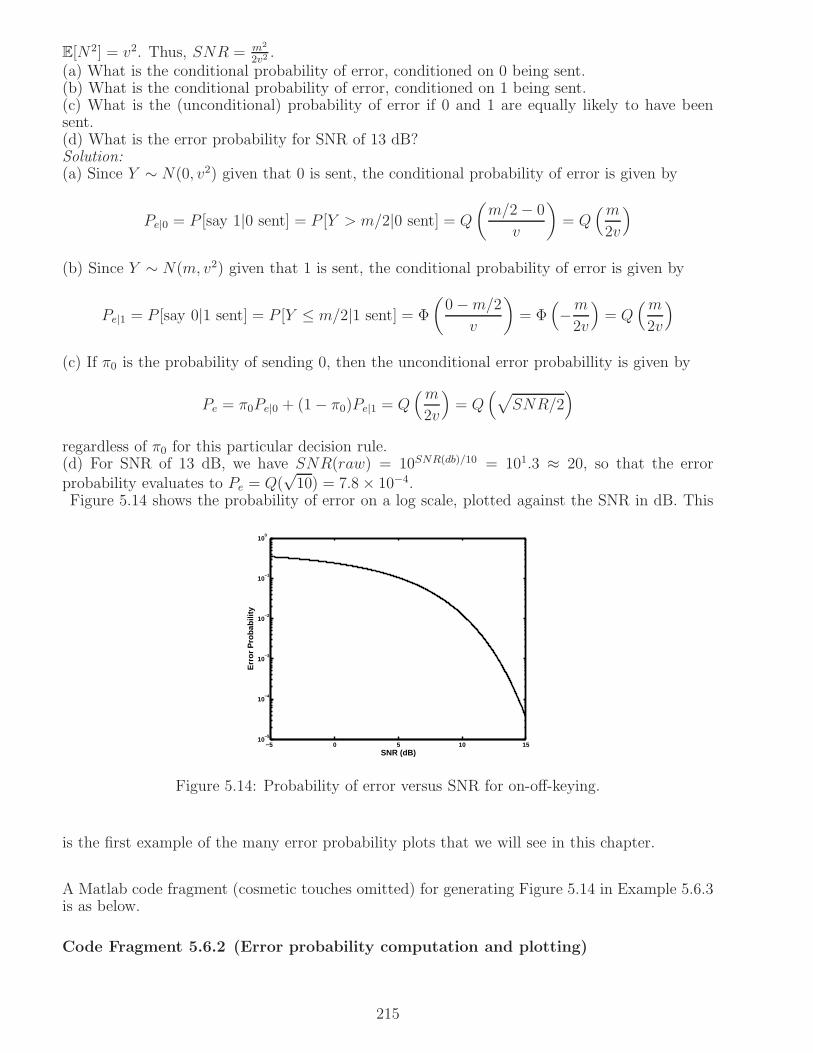
E[N2] = v2. Thus, SNR = m2

2v2.

(a) What is the conditional probability of error, conditioned on 0 being sent.(b) What is the conditional probability of error, conditioned on 1 being sent.(c) What is the (unconditional) probability of error if 0 and 1 are equally likely to have beensent.(d) What is the error probability for SNR of 13 dB?Solution:(a) Since Y ∼ N(0, v2) given that 0 is sent, the conditional probability of error is given by

Pe|0 = P [say 1|0 sent] = P [Y > m/2|0 sent] = Q

(

m/2− 0

v

)

= Q(m

2v

)

(b) Since Y ∼ N(m, v2) given that 1 is sent, the conditional probability of error is given by

Pe|1 = P [say 0|1 sent] = P [Y ≤ m/2|1 sent] = Φ

(

0−m/2

v

)

= Φ(

−m

2v

)

= Q(m

2v

)

(c) If π0 is the probability of sending 0, then the unconditional error probabillity is given by

Pe = π0Pe|0 + (1− π0)Pe|1 = Q(m

2v

)

= Q(

√

SNR/2)

regardless of π0 for this particular decision rule.(d) For SNR of 13 dB, we have SNR(raw) = 10SNR(db)/10 = 101.3 ≈ 20, so that the errorprobability evaluates to Pe = Q(

√10) = 7.8× 10−4.

Figure 5.14 shows the probability of error on a log scale, plotted against the SNR in dB. This

−5 0 5 10 1510

−5

10−4

10−3

10−2

10−1

100

Err

or P

roba

bilit

y

SNR (dB)

Figure 5.14: Probability of error versus SNR for on-off-keying.

is the first example of the many error probability plots that we will see in this chapter.

A Matlab code fragment (cosmetic touches omitted) for generating Figure 5.14 in Example 5.6.3is as below.

Code Fragment 5.6.2 (Error probability computation and plotting)

215

%Plot of error probability versus SNR for on-off keyingsnrdb = -5:0.1:15; %vector of SNRs (in dB) for which to evaluate error probsnr = 10.^(snrdb/10); %vector of raw SNRspe = qfunction(sqrt(snr/2)); %vector of error probabilities%plot error prob on log scale versus SNR in dBsemilogy(snrdb,pe);ylabel(’Error Probability’);xlabel(’SNR (dB)’);

The preceding example illustrates a more general observation for signaling in AWGN: the proba-bility of error involves terms such as Q(

√a SNR), where the scale factor a depends on properties

of the signal constellation, and SNR is the signal-to-noise ratio. It is therefore of interest to un-derstand how the error probability decays with SNR. As shown in Appendix 5.A, there are tightanalytical bounds for the Q function which can be used to deduce that it decays exponentiallywith its argument, as stated in the following.

Asymptotics of Q(x) for large arguments: For large x > 0, the exponential decay of the Qfunction dominates. We denote this by

Q(x).= e−x2/2 , x→ ∞ (5.53)

which is shorthand for the following limiting result:

limx→∞

logQ(x)

−x2/2 = 1 (5.54)

These asymptotics play a key role in design of communication systems. Since events that causebit errors have probabilities involving terms such as Q(

√a SNR)

.= e−a SNR/2, when there are

multiple events that can cause bit errors, the ones with the smallest rates of decay a dominateperformance. We can therefore focus on these worst-case events in our designs for moderate andhigh SNR. This simplistic view does not quite hold in heavily coded systems operating at lowSNR, but is still an excellent perspective for arriving at a coarse link design.

5.6.1 Joint Gaussianity

Often, we need to deal with multiple Gaussian random variables defined on the same probabilityspace. These might arise, for example, when we sample filtered WGN. In many situations ofinterest, not only are such random variables individually Gaussian, but they satisfy a strongerjoint Gaussianity property. Just as a Gaussian random variable is characterized by its mean andvariance, jointly Gaussian random variables are characterized by means and covariances. We arealso interested in what happens to these random variables under linear operations, corresponding,for example, to filtering. Hence, we first review mean and covariance, and their evolution underlinear operations and translations, for arbitrary random variables defined on the same probabilityspace.

Covariance: The covariance of random variables X1 and X2 measures the correlation betweenhow they vary around their means, and is given by

cov(X1, X2) = E [(X1 − E[X1])(X2 − E[X2])] = E[X1X2]− E[X1]E[X2]

The second formula is obtained from the first by multiplying out and simplifying:

E [(X1 − E[X1])(X2 − E[X2])] = E [X1X2 − E[X1]X2 + E[X1]E[X2]−X1E[X2]]= E[X1X2]− E[X1]E[X2] + E[X1]E[X2]− E[X1]E[X2] = E[X1X2]− E[X1]E[X2]

216

where we use the linearity of the expectation operator to pull out constants.

Uncorrelatedness: X1 and X2 are said to be uncorrelated if cov(X1, X2) = 0.

Independent random variables are uncorrelated: If X1 and X2 are independent, then

cov(X1, X2) = E[X1X2]− E[X1]E[X2] = E[X1]E[X2]− E[X1]E[X2] = 0

The converse is not true in general; that is, uncorrelated random variables need not be inde-pendent. However, we shall see that jointly Gaussian uncorrelated random variables are indeedindependent.

Variance: Note that the variance of a random variable is its covariance with itself:

var(X) = cov(X,X) = E[

(X − E[X ])2]

= E[X2]− (E[X ])2

The use of matrices and vectors provides a compact way of representing and manipulating meansand covariances, especially using software programs such as Matlab. Thus, for random variablesX1, ..., Xm, we define the random vector X = (X1, ..., Xm)

T , and arrange the means and pairwisecovariances in a vector and matrix, respectively, as follows.

Mean vector and covariance matrix: Consider an arbitrary m-dimensional random vectorX = (X1, ..., Xm)

T . The m×1 mean vector of X is defined as mX = E[X] = (E[X1], ...,E[Xm])T .

The m×m covariance matrix CX has (i, j)th entry given by the covariance between the ith andjth random variables:

CX(i, j) = cov(Xi, Xj) = E [(Xi − E[Xi])(Xj − E[Xj ])] = E [XiXj]− E[Xi]E[Xj ]

More compactly,

CX = E[(X− E[X])(X− E[X])T ] = E[XXT ]− E[X](E[X])T

Notes on covariance computation: Computations of variance and covariance come up oftenwhen we deal with Gaussian random variables, hence it is useful to note the following propertiesof covariance.Property 1: Covariance is unaffected by adding constants.

cov(X + a, Y + b) = cov(X, Y ) for any constants a, b

Covariance provides a measure of the correlation between random variables after subtracting outtheir means, hence adding constants to the random variables (which just translates their means)does not affect covariance.Property 2: Covariance is a bilinear function (i.e., it is linear in both its arguments).

cov(a1X1 + a2X2, a3X3 + a4X4) = a1a3cov(X1, X3) + a1a4cov(X1, X4)+ a2a3cov(X2, X3) + a2a4cov(X2, X4)

By Property 1, it is clear that we can always consider zero mean, or centered, versions of randomvariables when computing the covariance. An example that frequently arises in performanceanalysis of communication systems is a random variable which is a sum of a deterministic term(e.g., due to a signal), and a zero mean random term (e.g. due to noise). In this case, droppingthe signal term is often convenient when computing variance or covariance.

Affine transformations: For a random vector X, the analogue of scaling and translating arandom variable is a linear transformation using a matrix, together with a translation. Such atransformation is called an affine transformation. That is, Y = AX+b is an affine transformationof X, where A is a deterministic matrix and b a deterministic vector.

217

Example 5.6.4 (Mean and variance after an affine transformation): Let Y = X1 −2X2+4, where X1 has mean -1 and variance 4, X2 has mean 2 and variance 9, and the covariancecov(X1, X2) = −3. Find the mean and variance of Y .Solution: The mean is given by

E[Y ] = E[X1]− 2E[X2] + 4 = −1− 2(2) + 4 = −1

The variance is computed as

var(Y ) = cov(Y, Y ) = cov(X1 − 2X2 + 4, X1 − 2X2 + 4)= cov(X1, X1)− 2cov(X1, X2)− 2cov(X2, X1) + 4cov(X2, X2)

where the constant drops out because of Property 1. We therefore obtain that

var(Y ) = cov(X1, X1)− 4cov(X1, X2) + 4cov(X2, X2) = 4− 4(−3) + 4(9) = 52

Computations such as those in the preceding example can be compactly represented in termsof matrices and vectors, which is particularly useful for computations for random vectors. Ingeneral, an affine transformation maps one random vector into another (of possibly differentdimension), and the mean vector and covariance matrix evolve as follows.

Mean and covariance evolution under affine transformationIf X has mean m and covariance C, and Y = AX+ b,

then Y has mean mY = Am+ b and covariance CY = ACAT .

To see this, first compute the mean vector of Y using the linearity of the expectation operator:

mY = E[Y] = E[AX+ b] = AE[X] + b = Am+ b (5.55)

This also implies that the “zero mean” version of Y is given by

Y − E[Y] = (AX+ b)− (AmX + b) = A(X−mX)

so that the covariance matrix of Y is given by

CY = E[(Y − E[Y])(Y − E[Y])T ] = E[A(X−m)(X−m)TAT ] = ACAT (5.56)

Note that the dimensions of X and Y can be different: X can be m×1, A can be n×m, and Y,b can be n× 1, where m, n are arbitrary. We also note below that mean and covariance evolveseparately under such transformations.

Mean and covariance evolve separately under affine transformations: The mean of Ydepends only on the mean of X, and the covariance of Y depends only on the covariance of X.Furthermore, the additive constant b in the transformation does not affect the covariance, sinceit influences only the mean of Y.

Example 5.6.4 redone: We can check that we get the same result as before by setting

mX =

(

−12

)

, CX =

(

4 −3−3 9

)

(5.57)

A = (1 − 2) , b = 4

and applying (5.55) and (5.56).

Jointly Gaussian random variables, or Gaussian random vectors: Random variablesX1, ..., Xm defined on a common probability space are said to be jointly Gaussian, or the m× 1

218

random vector X = (X1, ..., Xm)T is termed a Gaussian random vector, if any linear combination

of these random variables is a Gaussian random variable. That is, for any scalar constantsa1, ..., am, the random variable a1X1 + ... + amXm is Gaussian.

A Gaussian random vector is completely characterized by its mean vector and co-variance matrix: This is a generalization of the observation that a Gaussian random variable iscompletely characterized by its mean and variance. We derive this in Problem 5.48, but providean intuitive argument here. The definition of joint Gaussianity only requires us to characterizethe distribution of an arbitrarily chosen linear combination of X1, ..., Xm. For a Gaussian randomvector X = (X1, ..., Xm)

T , consider Y = a1X1 + ... + amXm, where a1, ..., am can be any scalarconstants. By definition, Y is a Gaussian random variable, and is completely characterized byits mean and variance. We can compute these in terms of mX and CX using (5.55) and (5.56)by noting that Y = aTX, where a = (a1, ..., am)

T . Thus,

mY = aTmX

CY = var(Y ) = aTCXa

We have therefore shown that we can characterize the mean and variance, and hence the density,of an arbitrarily chosen linear combination Y if and only if we know the mean vector mX andcovariance matrix CX . As we see in Problem 5.48, this is the basis for the desired result thatthe distribution of Gaussian random vector X is completely characterized by mX and CX .

Notation for joint Gaussianity: We use the notation X ∼ N(m,C) to denote a Gaussianrandom vector X with mean vector m and covariance matrix C.

The preceding definitions and observations regarding joint Gaussianity apply even when therandom variables involved do not have a joint density. For example, it is easy to check that,according to this definition, X1 andX2 = 4X1−1 are jointly Gaussian. However, the joint densityof X1 and X2 is not well-defined (unless we allow delta functions), since all of the probabilitymass in the two-dimensional (x1, x2) plane is collapsed onto the line x2 = 4x1 − 1. Of course,since X2 is completely determined by X1, any probability involving X1, X2 can be expressed interms of X1 alone. In general, when the m-dimensional joint density does not exist, probabilitiesinvolving X1, ..., Xm can be expressed in terms of a smaller number of random variables, andcan be evaluated using a joint density over a lower-dimensional space. A necessary and sufficientcondition for the joint density to exist is that the covariance matrix is invertible.

Joint Gaussian density exists if and only if the covariance matrix is invertible: Wedo not prove this result, but discuss it in the context of the two-dimensional density in Example5.6.5.

Joint Gaussian density: For X = (X1, ..., Xm) ∼ N(m,C), if C is invertible, the joint densityexists and takes the following form (we skip the derivation, but see Problem 5.48):

p(x1, ..., xm) = p(x) =1

√

(2π)m|C|exp

(

−1

2(x−m)TC−1(x−m)

)

(5.58)

where |C| denotes the determinant of C.

Example 5.6.5 (Two-dimensional joint Gaussian density) In order to visualize the jointGaussian density (this is not needed for the remainder of the development, hence this examplecan be skipped), let us consider two jointly Gaussian random variables X and Y . In this case, itis convenient to define the normalized correlation between X and Y as

ρ(X, Y ) =cov(X, Y )

√

var(X)var(Y )(5.59)

219

−5

0

5

−5

0

50

0.02

0.04

0.06

0.08

0.1

xy

Join

t Gau

ssia

n D

ensi

ty

(a) Joint Gaussian Density

x

y

−5 −4 −3 −2 −1 0 1 2 3 4 5−5

−4

−3

−2

−1

0

1

2

3

4

5

(b) Contours of density

Figure 5.15: Joint Gaussian density and its contours for σ2X = 1, σ2

Y = 4 and ρ = −0.5.

Thus, cov(X, Y ) = ρσXσY , where var(X) = σ2X , var(Y ) = σ2

Y , and the covariance matrix for therandom vector (X, Y )T is given by

C =

(

σ2X ρσXσY

ρσXσY σ2Y

)

(5.60)

It is shown in Problem 5.47 that |ρ| ≤ 1. For |ρ| = 1, it is easy to check that the covariance matrixhas determinant zero, hence the joint density formula (5.58) cannot be applied. As shown inProblem 5.47, this has a simple geometric interpretation: |ρ| = 1 corresponds to a situation whenX and Y are affine functions of each other, so that all of the probability mass is concentratedon a line, hence a two-dimensional density does not exist. Thus, we need the strict inequality|ρ| < 1 for the covariance matrix to be invertible. Assuming that |ρ| < 1, we plug (5.60) into(5.58), setting the mean vector to zero without loss of generality (a nonzero mean vector simplyshifts the density). We get the joint density shown in Figure 5.15 for σ2

X = 1, σ2Y = 4 and

ρ = −0.5. Since Y has larger variance, the density decays more slowly in Y than in X . Thenegative normalized correlation leads to contour plots given by tilted ellipses, corresponding tosetting quadratic function xTC−1x in the exponent of the density to different constants.Exercise: Show that the ellipses shown in Figure 5.15(b) can be described as

x2 + ay2 + bxy = c

specifying the values of a and b.

While we hardly ever integrate the joint Gaussian density to compute probabilities, we use itsform to derive many important results. One such result is stated below.

Uncorrelated jointly Gaussian random variables are independent: This follows fromthe form of the joint Gaussian density (5.58). If X1, ..., Xm are pairwise uncorrelated, then theoff-diagonal entries of the covariance matrix C are zero: C(i, j) = 0 for i 6= j. Thus, C andC−1 are both diagonal matrices, with diagonal entries given by C(i, i) = v2i , C

−1(i, i) = 1v2i,

i = 1, ..., m, and determinant |C| = v21...v2m. In this case, we see that the joint density (5.58)

decomposes into a product of marginal densities:

p(x1, ..., xm) =1

√

2πv21e− (x1−m1)

2

2v21 ...1

√

2πv2me− (x1−mm)2

2v2m = p(x1)...p(xm)

220

so that X1, ..., Xm are independent.

Recall that, while independent random variables are uncorrelated, the converse need not be true.However, when we put the additional restriction of joint Gaussianity, uncorrelatedness does implyindependence.

We can now characterize the distribution of affine transformations of jointly Gaussian randomvariables. If X is a Gaussian random vector, then Y = AX + b is also Gaussian. To see this,note that any linear combination of Y1, ..., Yn equals a linear combination of X1, ..., Xm (plus aconstant), which is a Gaussian random variable by the Gaussianity of X. Since Y is Gaussian,its distribution is completely characterized by its mean vector and covariance matrix, which wehave just computed. We can now state the following result.

Joint Gaussianity is preserved under affine transformations

If X ∼ N(m,C), then AX+ b ∼ N(Am+ b,ACAT ) (5.61)

Example 5.6.6 (Computations with jointly Gaussian random variables) As in Example5.6.4, consider two random variables X1 and X2 such that X1 has mean -1 and variance 4, X2

has mean 2 and variance 9, and cov(X1, X2) = −3. Now assume in addition that these randomvariables are jointly Gaussian.(a) Write down the mean vector and covariance matrix for the random vector Y = (Y1, Y2)

T ,where Y1 = 3X1 −X2 + 3 and Y2 = X1 +X2 − 2.(b) Evaluate the probability P [3X1−X2 < 5] in terms of the Q function with positive arguments.(c) Suppose that Z = aX1 +X2. Find the constant a such that Z is independent of X1 +X2.Solution to (a): We have already found the mean and covariance of X in Example 5.6.4; theyare given by (5.57). Now, Y = AX+ b, where

A =

(

3 −21 1

)

, b =

(

3−2

)

We can now apply (5.61) to obtain the mean vector and covariance matrix for Y:

mY = AmX + b =

(

−4−1

)

CY = ACXAT =

(

108 −9−9 7

)

Solution to (b): Since Y1 = 3X1 −X2 + 3 ∼ N(−4, 108), the required probability can be writtenas

P [3X1 −X2 < 5] = P [Y1 < 8] = Φ

(

8− (−4)√108

)

= Φ(

2/√3)

= 1−Q(

2/√3)

Solution to (c): Since Z = aX1 +X2 and X1 are jointly Gaussian, they are independent if theyare uncorrelated. The covariance is given by

cov(Z,X1) = cov(aX1 +X2, X1) = a cov(X1, X1) + cov(X2, X1) = 4a− 3

so that we need a = 3/4 for Z and X1 to be independent.

Discrete time WGN: The noise model N ∼ N(0, σ2I) is called discrete time white Gaussiannoise (WGN). The term white refers to the noise samples being uncorrelated and having equalvariance. We will see how such discrete time WGN arises from continuous-time WGN, which wediscuss during our coverage of random processes later in this chapter.

221

Example 5.6.7 (Binary on-off keying in discrete time WGN) Let us now revisit on-offkeying, explored for scalar observations in Example 5.6.3, for vector observations. The receiverprocesses a vector Y = (Y1, ..., Yn)

T of samples modeled as follows: Y = s +N if 1 is sent, andY = N is 0 is sent, where s = (s1, ..., sn)

T is the signal, and the noise N = (N1, ..., Nn)T ∼

N(0, σ2I). That is, the noise samples N1, ..., Nn are i.i.d. N(0, σ2) random variables. Supposewe use the following correlator-based decision statistic:

Z = sTY =

n∑

k=1

skYk

Thus, we have reduced the vector observation to a single number based on which we will makeour decision. The hypothesis framework developed in Chapter 6 will be used to show that thisdecision statistic is optimal, in a well-defined sense. For now, we simply accept it as given.(a) Find the conditional distribution of Z given that 0 is sent.(b) Find the conditional distribution of Z given that 1 is sent.(c) Observe from (a) and (b) that we are now back to the setting of Example 5.6.3, with Z now

playing the role of Y . Specify the values of m and v2, and the SNR = m2

2v2, in terms of s and σ2.

(d) As in Example 5.6.3, consider the simple decision rule that 1 is sent if Z > m/2, and saythat 0 is sent if Z ≤ m/2. Find the error probability (in terms of the Q function) as a functionof s and σ2.(e) Evaluate the error probability for s = (−2, 2, 1)T and σ2 = 1/4.Solution:(a) If 0 is sent, then Y = N =∼ N(0, σ2I). Applying (5.61) with m = 0, A = sT , C = σ2I, weobtain Z = sTY ∼ N(0, σ2||s||2).(b) If 1 is sent, then Y = s + N ∼ N(s, σ2I). Applying (5.61) with m = s, A = sT , C = σ2I,we obtain Z = sTY ∼ N(||s||2, σ2||s||2). Alternatively, sTY = sT (s +N) = ||s||2 + sTN. SincesTN ∼ N(0, σ2||s||2) from (a), we simply translate the mean by ||s||2.(c) Comparing with Example 5.6.3, we see that m = ||s||2, v2 = σ2||s||2, and SNR = m2

2v2= ||s||2

2σ2 .(d) From Example 5.6.3, we know that the decision rule that splits the difference between themeans has error probability

Pe = Pe|0 = Pe|1 = Q(m

2v

)

= Q

( ||s||2σ

)

plugging in the expressions for m and v2 from (c). (e) We have ||s||2 = 9. Using (d), we obtainPe = Q(3) = 0.0013.

Noise is termed colored when it is not white; that is, when the noise samples are correlated and/orhave different variances. We will see later how colored noise arises from linear transformationson white noise. Let us continue our sequence of examples regarding on-off keying, but now withcolored noise.

Example 5.6.8 (Binary on-off keying in discrete time colored Gaussian noise) As inthe previous example, we have a vector observation Y = (Y1, ..., Yn)

T , with Y = s + N if 1 issent, and Y = N is 0 is sent, where s = (s1, ..., sn)

T is the signal. However, we now allow thenoise covariance matrix to be arbitrary: N = (N1, ..., Nn)

T ∼ N(0,CN ).(a) Consider the decision statistic Z1 = sTY. Find the conditional distributions of Z1 given 0sent, and given 1 sent.(b) Show that Z1 follows the scalar on-off keying model Example 5.6.3, specifying the parameters

m1 and v21, and SNR1 =m2

1

2v21, in terms of s and CN .

(c) Find the error probability of the simple decision rule comparing Z1 to the threshold m1/2.

222

(d) Repeat (a)-(c) for an decision statistic Z2 = sTC−1N Y (use the notation m2, v

22 and SNR2 to

denote the quantities analogous to those in (b)).(e) Apply the preceding to the following example: two-dimensional observation Y = (Y1, Y2)with s = (4,−2)T and

CN =

(

1 −1−1 4

)

Find explicit expressions for Z1 and Z2 in terms of Y1 and Y2. Compute and compare the SNRsand error probabilities obtained with the two decision statistics.Solution: We proceed similarly to Example 5.6.7.(a) If 0 is sent, then Y = N =∼ N(0,CN). Applying (5.61) with m = 0, A = sT , C = CN , weobtain Z1 = sTY ∼ N(0, sTCNs).If 1 is sent, then Y = s +N ∼ N(s,CN). Applying (5.61) with m = s, A = sT , C = CN , weobtain Z1 = sTY ∼ N(||s||2, sTCNs). Alternatively, sTY = sT (s + N) = ||s||2 + sTN. SincesTN ∼ N(0, sTCNs) from (a), we simply translate the mean by ||s||2.(b) Comparing with Example 5.6.3, we see that m1 = ||s||2, v21 = sTCNs, and SNR1 =

m21

2v21=

||s||22sTCNs

.

(c) From Example 5.6.3, we know that the decision rule that splits the difference between themeans has error probability

Pe1 = Q

(

m1

2v1

)

= Q

( ||s||22√sTCNs

)

plugging in the expressions for m1 and v21 from (b).(d) We now have Z2 = sTC−1

N Y. If 0 is sent, Y = N =∼ N(0,CN). Applying (5.61) with m = 0,A = sTC−1

N , C = CN , we obtain Z2 = sTY ∼ N(0, sTC−1N s).

If 1 is sent, then Y = s +N ∼ N(s,CN ). Applying (5.61) with m = s, A = sTC−1N , C = CN ,

we obtain Z2 = sTC−1N Y ∼ N(sTC−1

N s, sTC−1N s). That is, m2 = sTC−1

N s, v22 = sTC−1N s, and

SNR2 =m2

2

2v22=

sTC−1N s

2. The corresponding error probability is Pe2 = Q

(

m2

2v2

)

= Q

(√sTC

−1N s

2

)

(e) For the given example, we find Z1 = sTY = 4Y1 − 2Y2 and Z2 = sTC−1N Y = 2

3(7Y1 + Y2).

We can see that the relative weights of the two observations are quite different in the two cases.Numerical computations using the Matlab script below yield SNRs of 6.2 dB and 9.4 dB, anderror probabilities of 0.07 and 0.02 in the two cases, so that Z2 provides better performance thanZ1. We shall see in Chapter 6 that Z2 is actually the optimal decision statistic, both in terms ofmaximizing SNR and minimizing error probability.

A Matlab code fragment for generating the numerical results in Example 5.6.8(e) is given below.

Code Fragment 5.6.3 (Performance of on-off keying in colored Gaussian noise)

%%OOK with colored noise: N(s,C_N) versus N(0,C_N)s=[4;-2]; %signalCn=[1 -1;-1 4]; %noise covariance matrix%%decision statistic Z1 = s^T Ym1= s’*s; %mean if 1 sentvariance1 =s’*Cn*s; %variance under each hypothesisv1=sqrt(variance1); %standard deviationSNR1 = m1^2/(2*variance1); %SNRPe1 = qfunction(m1/(2*v1)); %error prob for "split the difference" rule using Z1%%decision statistic Z2 = s^T Cn^-1 Y

223

m2 = s’*inv(Cn)*s; %mean if 1 sentvariance2=s’*inv(Cn)*s; %variance=mean in this casev2=sqrt(variance2); %standard deviationSNR2 = m2^2/(2*variance2); %reduces to SNR2= m2/2 in this casePe2 = qfunction(m2/(2*v2)); %error prob for "split the difference" rule using Z2%Compare performance of the two rules10*log10([SNR1 SNR2]) %SNRs in dB[Pe1 Pe2] %error probabilities

5.7 Random Processes

A key limitation on the performance of communication systems comes from receiver noise, whichis an unavoidable physical phenomenon (see Appendix 5.C). Noise cannot be modeled as adeterministic waveform (i.e., we do not know what noise waveform we will observe at any givenpoint of time). Indeed, neither can the desired signals in a communication system, even thoughwe have sometimes pretended otherwise in prior chapters. Information-bearing signals suchas speech, audio, video are best modeled as being randomly chosen from a vast ensemble ofpossibilities. Similarly, the bit stream being transmitted in a digital communication system canbe arbitrary, and can therefore be thought of as being randomly chosen from a large number ofpossible bit streams. It is time, therefore, to learn how to deal with random processes, which isthe technical term we use for signals that are chosen randomly from an ensemble, or collection, ofpossible signals. A detailed investigation of random processes is well beyond our scope, and ourgoal here is limited to developing a working understanding of concepts critical to our study ofcommunication systems. We shall see that this goal can be achieved using elementary extensionsof the probability concepts covered earlier in this chapter.

5.7.1 Running example: sinusoid with random amplitude and phase

Let us work through a simple example before we embark on a systematic development. Supposethat X1 and X2 are i.i.d. N(0, 1) random variables, and define

X(t) = X1 cos 2πfct−X2 sin 2πfct (5.62)

where fc > 0 is a fixed frequency. The waveform X(t) is not a deterministic signal, sinceX1 and X2 can take random values on the real line. Indeed, for each time t, X(t) is a randomvariable, since it is a linear combination of two random variables X1 and X2 defined on a commonprobability space. Moreover, if we pick a number of times t1, t2, ..., then the correspondingsamples X(t1), X(t2), ... are random variables on a common probability space.

Another interpretation of X(t) is obtained by converting (X1, X2) to polar form:

X1 = A cosΘ , X2 = A sinΘ

For X1, X2 i.i.d. N(0, 1), we know from Problem 5.21 that A is Rayleigh, Θ is uniform over[0, 2π], and A, Θ are independent. The random process X(t) can be rewritten as

X(t) = A cosΘ cos 2πfct− A sinΘ sin 2πfct = A cos(2πfct +Θ) (5.63)

Thus, X(t) is a sinusoid with random amplitude and phase.

For a given time t, what is the distribution of X(t)? Since X(t) is a linear combination of i.i.d.Gaussian, hence jointly Gaussian, random variables X1 and X2, we infer that it is a Gaussian

224

random variable. Its distribution is therefore specified by computing its mean and variance, asfollows:

E [X(t)] = E[X1] cos 2πfct− E[X2] sin 2πfct = 0 (5.64)

var (X(t)) = cov (X1 cos 2πfct−X2 sin 2πfct, X1 cos 2πfct−X2 sin 2πfct)= cov(X1, X1) cos

2 2πfct + cov(X2, X2) sin2 2πfct− 2cov(X1, X2) cos 2πfct sin 2πfct

= cos2 2πfct+ sin2 2πfct = 1(5.65)

using cov(Xi, Xi) = var(Xi) = 1, i = 1, 2, and cov(X1, X2) = 0 (since X1, X2 are independent).Thus, we have X(t) ∼ N(0, 1) for any t.

In this particular example, we can also easily specify the joint distribution of any set of n samples,X(t1), ..., X(tn), where n can be arbitrarily chosen. The samples are jointly Gaussian, since theyare linear combinations of the jointly Gaussian random variables X1, X2. Thus, we only need tospecify their means and pairwise covariances. We have just shown that the means are zero, andthat the diagonal entries of the covariance matrix are one. More generally, the covariance of anytwo samples can be computed as follows:

cov (X(ti), X(tj)) = cov (X1 cos 2πfcti −X2 sin 2πfcti, X1 cos 2πfctj −X2 sin 2πfctj)= cov(X1, X1) cos 2πfcti cos 2πfctj + cov(X2, X2) sin 2πfcti sin 2πfctj

− 2cov(X1, X2) cos 2πfcti sin 2πfctj= cos 2πfcti cos 2πfctj + sin 2πfcti sin 2πfctj= cos 2πfc(ti − tj)

(5.66)

While we have so far discussed the random process X(t) from a statistical point of view, forfixed values of X1 and X2, we see that X(t) is actually a deterministic signal. Specifically, if therandom vector (X1, X2) is defined over a probability space Ω, a particular outcome ω ∈Ω mapsto a particular realization (X1(ω), X2(ω)). This in turn maps to a deterministic “realization,” or“sample path,” of X(t), which we denote as X(t, ω):

X(t, ω) = X1(ω) cos 2πfct−X2(ω) sin 2πfct

To see what these sample paths look like, it is easiest to refer to the polar form (5.63):

X(t, ω) = A(ω) cos (2πfct+Θ(ω))

Thus, as shown in Figure 5.16, different sample paths have different amplitudes, drawn from aRayleigh distribution, along with phase shifts drawn from a uniform distribution.

5.7.2 Basic definitions

As we have seen earlier, a random vector X = (X1, ..., Xn)T is a finite collection of random

variables defined on a common probability space, as depicted in Figure 5.7. A random processis simply a generalization of this concept, where the number of such random variables can beinfinite.

Random process: A random process X is a collection of random variables X(t), t∈T , wherethe index set T can be finite, countably infinite, or uncountably infinite. When we interpret theindex set as denoting time, as we often do for the scenarios of interest to us, a countable indexset corresponds to a discrete time random process, and an uncountable index set corresponds toa continuous time random process. We denote by X(t, ω) the value taken by the random variableX(t) for any given outcome ω in the sample space.

225

0 0.5 1 1.5 2 2.5 3 3.5 4−1.5

−1

−0.5

0

0.5

1

1.5

t

Figure 5.16: Two sample paths for a sinusoid with random amplitude and phase.

For the sinusoid with random amplitude and phase, the sample space only needs to be richenough to support the two random variables X1 and X2 (or A and Θ), from which we can createa continuum of random variables X(t, ω), −∞ < t <∞:

ω → (X1(ω), X2(ω)) → X(t, ω)

In general, however, the source of randomness can be much richer. Noise in a receiver circuit iscaused by random motion of a large number of charge carriers. A digitally modulated waveformdepends on a sequence of randomly chosen bits. The preceding conceptual framework is generalenough to cover all such scenarios.

Sample paths: We can also interpret a random process as a signal drawn at random from anensemble, or collection, of possible signals. The signal we get at a particular random draw iscalled a sample path, or realization, of the random process. Once we fix a sample path, it can betreated like a deterministic signal. Specifically, for each fixed outcome ω ∈Ω, the sample pathis X(t, ω), which varies only with t. We have already seen examples of samples paths for ourrunning example in Figure 5.16.

Finite-dimensional distributions: As indicated in Figure 5.17, the samples X(t1), ..., X(tn)from a random process X are mappings from a common sample space to the real line, withX(ti, ω) denoting the value of the random variableX(ti) for outcome ω ∈Ω. The joint distributionof these random variables depends on the underlying probability measure on the sample spaceΩ. We say that we “know” the statistics of a random process if we know the joint statistics ofan arbitrarily chosen finite collection of samples. That is, we know the joint distribution of thesamples X(t1), ..., X(tn), regardless of the number of samples n, and the sampling times t1, ..., tn.These joint distributions are called the finite-dimensional distributions of the random process,with the joint distribution of n samples called an nth order distribution. Thus, while a randomprocess may be comprised of infinitely many random variables, when we specify its statistics, wefocus on a finite subset of these random variables.

For our running example (5.62), we observed that the samples are jointly Gaussian, and specifiedthe joint distribution by computing the means and covariances. This is a special case of a broaderclass of Gaussian random processes (to be defined shortly) for which it is possible to characterizefinite-dimensional distributions compactly in this fashion. Often, however, it is not possible toexplicitly specify such distributions, but we can still compute useful quantities averaged across

226

n

1

X (t )2

X (t , )ω2

1X (t , )ω

Ω

ω

Sample space

ωX (t , )n

X (t )

X (t )

Figure 5.17: Samples of a random process are random variables defined on a common probabilityspace.

sample paths.

Ensemble averages: Knowing the finite-dimensional distributions enables us to compute sta-tistical averages across the collection, or ensemble, of sample paths. Such averages are calledensemble averages. We will be mainly interested in “second order” statistics (involving expecta-tions of products of at most two random variables), such as means and covariances. We definethese quantities in sufficient generality that they apply to complex-valued random processes, butspecialize to real-valued random processes in most of our computations.

5.7.3 Second order statistics

Mean, autocorrelation, and autocovariance functions (ensemble averages): For a ran-dom process X(t), the mean function is defined as

mX(t) = E[X(t)] (5.67)

and the autocorrelation function as

RX(t1, t2) = E[X(t1)X∗(t2)] (5.68)

Note that RX(t, t) = E[|X(t)|2] is the instantaneous power at time t. The autocovariance functionof X is the autocorrelation function of the zero mean version of X , and is given by

CX(t1, t2) = E[(X(t1)− E[X(t1)])(X(t2)− E[X(t2)])∗] = RX(t1, t2)−mX(t1)m

∗X(t2) (5.69)

Second order statistics for running example: We have from (5.64) and (5.66) that

mX(t) ≡ 0 , CX(t1, t2) = RX(t1, t2) = cos 2πfc(t1 − t2) (5.70)

It is interesting to note that the mean function does not depend on t, and that the autocorrelationand autocovariance functions depend only on the difference of the times t1 − t2. This impliesthat if we shift X(t) by some time delay d, the shifted process X(t) = X(t− d) would have thesame mean and autocorrelation functions. Such translation invariance of statistics is interestingand important enough to merit a formal definition, which we provide next.

227

5.7.4 Wide Sense Stationarity and Stationarity

Wide sense stationary (WSS) random process: A random process X is said to be WSS if

mX(t) ≡ mX(0) for all t

andRX(t1, t2) = RX(t1 − t2, 0) for all t1, t2

In this case, we change notation, dropping the time dependence in the notation for the meanmX , and expressing the autocorrelation function as a function of τ = t1 − t2 alone. Thus, for aWSS process, we can define the autocorrelation function as

RX(τ) = E[X(t)X∗(t− τ)] for X WSS (5.71)

with the understanding that the expectation is independent of t. Since the mean is independentof time and the autocorrelation depends only on time differences, the autocovariance also dependsonly on time differences, and is given by

CX(τ) = RX(τ)− |mX |2 for X WSS (5.72)

Second order statistics for running example (new notation): With this new notation,we have

mX ≡ 0 , RX(τ) = CX(τ) = cos 2πfcτ (5.73)

A WSS random process has shift-invariant second order statistics. An even stronger notion ofshift-invariance is stationarity.

Stationary random process: A random processX(t) is said to be stationary if it is statisticallyindistinguishable from a delayed version of itself. That is, X(t) and X(t − d) have the samestatistics for any delay d∈ (−∞,∞).

Running example: The sinusoid with random amplitude and phase in our running example isstationary. To see this, it is convenient to consider the polar form in (5.63): X(t) = A cos(2πfct+Θ), where Θ is uniformly distributed over [0, 2π]. Note that

Y (t) = X(t− d) = A cos(2πfc(t− d) + Θ) = A cos(2πfct+Θ′)

where Θ′ = Θ − 2πfcd modulo 2π is uniformly distributed over [0, 2π]. Thus, X and Y arestatistically indistinguishable.

Stationarity implies wide sense stationarity: For a stationary random process X , the meanfunction satisfies

mX(t) = mX(t− d)

for any t, regardless of the value of d. Choosing d = t, we infer that

mX(t) = mX(0) (5.74)

That is, the mean function is a constant. Similarly, the autocorrelation function satisfies

RX(t1, t2) = RX(t1 − d, t2 − d)

for any t1, t2, regardless of the value of d. Setting d = t2, we have that

RX(t1, t2) = RX(t1 − t2, 0) (5.75)

Thus, a stationary process is also WSS.

While our running example was easy to analyze, in general, stationarity is a stringent requirementthat is not easy to verify. For our needs, the weaker concept of wide sense stationarity typicallysuffices. Further, we are often interested in Gaussian random processes (defined shortly), forwhich wide sense stationarity actually implies stationarity.

228

5.7.5 Power Spectral Density

Meter

∆

f∆S ( )x f*

H(f)

x(t)

1

f*

Power

f

Figure 5.18: Operational definition of PSD for a sample path x(t).

We have defined the concept of power spectral density (PSD), which specifies how the power ina signal is distributed in different frequency bands, for deterministic signals in Chapter 2. Thisdeterministic framework directly applies to a given sample path of a random process, and indeed,this is what we did when we computed the PSD of digitally modulated signals in Chapter 4.While we did not mention the term “random process” then (for the good reason that we hadnot introduced it yet), if we model the information encoded into a digitally modulated signal asrandom, then the latter is indeed a random process. Let us now begin by restating the definitionof PSD in Chapter 2.

Power Spectral Density: The power spectral density (PSD), Sx(f), for a finite-power signalx(t), which we can now think of as a sample path of a random process, is defined through theconceptual measurement depicted in Figure 5.18. Pass x(t) through an ideal narrowband filterwith transfer function

Hν(f) =

1, ν − ∆f2< f < ν + ∆f

2

0, else

The PSD evaluated at ν, Sx(ν), is defined as the measured power at the filter output, dividedby the filter width ∆f (in the limit as ∆f → 0).

The power meter in Figure 5.18 is averaging over time to estimate the power in a frequency sliceof a particular sample path. Let us review how this is done before discussing how to averageacross sample paths to define PSD in terms of an ensemble average.

Periodogram-based PSD estimation: The PSD can be estimated by computing Fouriertransform over a finite observation interval, and dividing its magnitude squared (which is theenergy spectral density) by the length of the observation interval. The time-windowed version ofx is defined as

xTo(t) = x(t)I[−To2,To

2](t) (5.76)

where To is the length of the observation interval. The Fourier transform of xTo(t) is denoted as

XTo(f) = F(xTo)

The energy spectral density of xTo is therefore |XTo(f)|2, and the PSD estimate is given by

Sx(f) =|XTo(f)|2

To(5.77)

PSD for a sample path: Formally, we define the PSD for a sample path in the limit of largetime windows as follows:

Sx(f) = limTo→∞

|XTo(f)|2To

PSD for sample path (5.78)

229

The preceding definition involves time averaging across a sample path, and can be related to thetime-averaged autocorrelation function, defined as follows.

Time-averaged autocorrelation function for a sample path: For a sample path x(t), wedefine the time-averaged autocorrelation function as

Rx(τ) = x(t)x∗(t− τ) = limTo→∞

1

To

∫ To2

−To2

x(t)x∗(t− τ) dt

We now state the following important result.

Time-averaged PSD and autocorrelation function form a Fourier transform pair.

Sx(f) ↔ Rx(τ) (5.79)

We omit the proof, but the result can be derived using the techniques of Chapter 2.

Time-averaged PSD and autocorrelation function for running example: For our ran-dom sinusoid (5.63), the time averaged autocorrelation function is given by

Rx(τ) = A cos(2πfct +Θ)A cos(2πfc(t− τ) + Θ)

= A2

2cos 2πfcτ + cos(4πfct− 2πfcτ + 2Θ)

= A2

2cos 2πfcτ

(5.80)

The time averaged PSD is given by

Sx(f) =A2

4δ(f − fc) +

A2

4δ(f + fc) (5.81)

We now extend the concept of PSD to a statistical average as follows.

Ensemble-averaged PSD: The ensemble-averaged PSD for a random process is defined asfollows:

SX(f) = limTo→∞

E

[ |XTo(f)|2To

]

ensemble averaged PSD (5.82)

That is, we take the expectations of the PSD estimates computed over an observation interval,and then let the observation interval get large.

Potential notational confusion: We use capital letters (e.g., X(t)) to denote a random processand small letters (e.g., x(t)) to denote sample paths. However, we also use capital letters todenote the Fourier transform of a time domain signal (e.g., s(t) ↔ S(f)), as introduced inChapter 2. Rather than introducing additional notation to resolve this potential ambiguity, werely on context to clarify the situation. In particular (5.82) illustrates this potential problem. Onthe left-hand side, we use X to denote the random process whose PSD SX(f) we are interested in.On the right-hand side, we use XTo(f) to denote the Fourier transform of a windowed sample pathxTo(t). Such opportunities for confusion arise seldom enough that it is not worth complicatingour notation to avoid them.

A result analogous to (5.79) holds for ensemble-averaged quantities as well.

Ensemble-averaged PSD and autocorrelation function for WSS processes form aFourier transform pair (Wiener-Khintchine theorem). For a WSS process X with auto-correlation function RX(τ), the ensemble averaged PSD is the Fourier transform of the ensemble-averaged autocorrelation function:

SX(f) = F (RX(τ)) =

∫ ∞

−∞RX(τ)e

−j2πfτ dτ (5.83)

230

This result is called the Wiener-Khintchine theorem, and can be proved under mild conditionson the autocorrelation function (the area under |RX(τ)| must be finite and its Fourier transformmust exist). The proof requires advanced probability concepts beyond our scope here, and isomitted.

Ensemble-averaged PSD for running example: For our running example, the PSD isobtained by taking the Fourier transform of (5.73):

SX(f) =1

2δ(f − fc) +

1

2δ(f + fc) (5.84)

That is, the power in X is concentrated at ±fc, as we would expect for a sinusoidal signal atfrequency fc.

Power: It follows from the Wiener-Khintchine theorem that the power of X can be obtainedeither by integrating the PSD or evaluating the autocorrelation function at τ = 0:

PX = E[X2(t)] = RX(0) =

∫ ∞

−∞SX(f)df (5.85)

For our running example, we obtain from (5.73) or (5.84) that PX = 1.

Ensemble versus Time Averages: For our running example, we computed the ensemble-averaged autocorrelation function RX(τ) and then used the Wiener-Khintchine theorem to com-pute the PSD by taking the Fourier transform. At other times, it is convenient to apply theoperational definition depicted in Figure 5.18, which involves averaging across time for a givensample path. If the two approaches give the same answer, then the random process is said to beergodic in PSD. In practical terms, ergodicity means that designs based on statistical averagesacross sample paths can be expected to apply to individual sample paths, and that measure-ments carried out on a particular sample path can serve as a proxy for statistical averagingacross multiple realizations.

Comparing (5.81) and (5.84), we see that our running example is actually not ergodic in PSD.For any sample path x(t) = A cos(2πfct+ θ), it is quite easy to show that

Sx(f) =A2

2δ(f − fc) +

A2

2δ(f + fc) (5.86)

Comparing with (5.84), we see that the time-averaged PSD varies across sample paths due toamplitude variations, with A2 replaced by its expectation in the ensemble-averaged PSD.

Intuitively speaking, ergodicity requires sufficient richness of variation across time and samplepaths. While this is not present in our simple running example (a randomly chosen amplitudewhich is fixed across the entire sample path is the culprit), it is often present in the morecomplicated random processes of interest to us, including receiver noise and digitally modulatedsignals (under appropriate conditions on the transmitted symbol sequences). When ergodicityholds, we have our choice of using either time averaging or ensemble averaging for computations,depending on which is most convenient or insightful.

The autocorrelation function and PSD must satisfy the following structural properties (theseapply to ensemble averages for WSS processes, as well as to time averages, although our notationcorresponds to ensemble averages).

Structural properties of PSD and autocorrelation function(P1) SX(f) ≥ 0 for all f .This follows from the sample path based definition in Figure 5.18, since the output of the powermeter is always nonnegative. Averaging across sample paths preserves this property.

231

(P2a) The autocorrelation function is conjugate symmetric: RX(τ) = R∗X(−τ).

This follows quite easily from the definition (5.71). By setting t = u+ τ , we have

RX(τ) = E[X(u+ τ)X∗(u)] = (E[X(u)X∗(u+ τ)])∗ = R∗X(−τ)

(P2b) For real-valued X , both the autocorrelation function and PSD are symmetric and real-valued. SX(f) = SX(−f) and RX(τ) = RX(−τ).(This is left as an exercise.)

Any function g(τ) ↔ G(f) must satisfy these properties in order to be a valid autocorrelationfunction/PSD.

Example 5.7.1 (Which function is an autocorrelation?) For each of the following func-tions, determine whether it is a valid autocorrelation function.(a) g1(τ) = sin(τ), (b) g2(τ) = I[−1,1](τ), (c) g3(τ) = e−|τ |

Solution(a) This is not a valid autocorrelation function, since it is not symmetric and violates property(P2b).(b) This satisfies Property (P2b). However, I[−1,1](τ) ↔ 2sinc(2f), so that Property (P1) isviolated, since the sinc function can take negative values. Hence, the boxcar function cannot bea valid autocorrelation function. This example shows that non-negativity Property P1 places astronger constraint on the validity of a proposed function as an autocorrelation function thanthe symmetry Property P2.(c) The function g3(τ) is symmetric and satisfies Property (P2b). It is left as an exercise to checkthat G3(f) ≥ 0, hence Property (P1) is also satisfied.

Units for PSD: Power per unit frequency has the same units as power multiplied by time, orenergy. Thus, the PSD is expressed in units of Watts/Hertz, or Joules.

−ν

∆f∆

f∆f∆ f∆

+

= x

x νν

S ( )

S (− ) + xS ( )νx(t) Power Meter

real−valued

H(f)

1

real−valued impulse response

ν

f

Figure 5.19: Operational definition of one-sided PSD.

One-sided PSD: The PSD that we have talked about so far is the two-sided PSD, which spansboth positive and negative frequencies. For a real-valued X , we can restrict attention to positivefrequencies alone in defining the PSD, by virtue of property (P2b). This yields the one-sidedPSD S+

X(f), defined as

S+X(f) = SX(f) + SX(−f) = 2SX(f) , f ≥ 0, (X(t) real) (5.87)

It is useful to interpret this in terms of the sample path based operational definition shown inFigure 5.19. The signal is passed through a physically realizable filter (i.e., with real-valuedimpulse response) of bandwidth ∆f , centered around ν. The filter transfer function must beconjugate symmetric, hence

Hν(f) =

1, ν − ∆f2< f < ν + ∆f

2

1, −ν − ∆f2< f < −ν + ∆f

2

0, else

232

The one-sided PSD is defined as the limit of the power of the filter output, divided by ∆f , as∆f → 0. Comparing Figures 5.18 and 5.19, we have that the sample path based one-sided PSDis simply twice the two-sided PSD: S+

x (f) = (Sx(f) + Sx(−f)) If≥0 = 2Sx(f)If≥0.

One-sided PSD for running example: From (5.84), we obtain that

S+X(f) = δ(f − fc) (5.88)

with all the power concentrated at fc, as expected.

Power in terms of PSD: We can express the power of a real-valued random process in termsof either the one-sided or two-sided PSD:

E[X2(t)] = RX(0) =

∫ ∞

−∞SX(f)df = (for X real)

∫ ∞

0

S+X(f)df (5.89)

Baseband and passband random processes: A random process X is baseband if its PSDis baseband, and is passband if its PSD is passband. Thinking in terms of time averaged PSDs,which are based on the Fourier transform of time windowed sample paths, we see that a randomprocess is baseband if its sample paths, time windowed over a large enough observation interval,are (approximately) baseband. Similarly, a random process is passband if its sample paths,time windowed over a large enough observation interval, are (approximately) passband. Thecaveat of “large enough observation interval” is inserted because of the following consideration:timelimited signals cannot be strictly bandlimited, but as long as the observation interval is largeenough, the time windowing (which corresponds to convolving the spectrum with a sinc function)does not spread out the spectrum of the signal significantly. Thus, the PSD (which is obtainedtaking the limit of large observation intervals) also defines the frequency occupancy of the samplepaths over large enough observation intervals. Note that these intuitions, while based on timeaveraged PSDs, also apply when bandwidth occupancy is defined in terms of ensemble-averagedPSDs, as long as the random process is ergodic in PSD.

2W

S (f)

Wf

−W

C

~~~~

S (f)up

PSD of DSB−SC signalMessage PSD

ff−f0 0

C/4

m

Figure 5.20: The relation between the PSDs of a message and the corresponding DSB-SC signal.

Example (PSD of a modulated passband signal): Consider a passband signal up(t) =m(t) cos 2πf0t, where m(t) is a message modeled as a baseband random process with PSD Sm(f)and power Pm. Timelimiting to an interval of length To and going to the frequency domain, wehave

Up,To(f) =1

2(MTo(f − f0) +MTo(f − f0)) (5.90)

Taking the magnitude squared, dividing by To, and letting To get large, we obtain

Sup(f) =1

4(Sm(f − f0) + Sm(f + f0)) (5.91)

An example is shown in Figure 5.20.

233

Thus, we start with the formula (5.90) relating the Fourier transform for a given sample path,which is identical to what we had in Chapter 2 (except that we now need to time limit the finitepower message to obtain a finite energy signal), and obtain the relation (5.91) relating the PSDs.An example is shown in Figure 5.20. We can now integrate the PSDs to get

Pu =1

4(Pm + Pm) =

Pm

2

5.7.6 Gaussian random processes

Gaussian random processes are just generalizations of Gaussian random vectors to an arbitrarynumber of components (countable or uncountable).

Gaussian random process: A random process X = X(t), t∈T is said to be Gaussian ifany linear combination of samples is a Gaussian random variable. That is, for any number n ofsamples, any sampling times t1, ..., tn, and any scalar constants a1, ..., an, the linear combinationa1X(t1)+ ...+anX(tn) is a Gaussian random variable. Equivalently, the samples X(t1), ..., X(tn)are jointly Gaussian.

Our running example (5.62) is a Gaussian random process, since any linear combination ofsamples is a linear combination of the jointly Gaussian random variables X1 and X2, and istherefore a Gaussian random variable.

A linear combination of samples from a Gaussian random process is completely characterized byits mean and variance. To compute the latter quantities for an arbitrary linear combination, wecan show, as we did for random vectors, that all we need to know are the mean function (analogousto the mean vector) and the autocovariance function (analogous to the covariance matrix) of therandom process. These functions therefore provide a complete statistical characterization of aGaussian random process, since the definition of a Gaussian random process requires only thatwe be able to characterize the distribution of an arbitrary linear combination of samples.

Characterizing a Gaussian random process: The statistics of a Gaussian random processare completely specified by its mean function mX(t) = E[X(t) and its autocovariance functionCX(t1, t2) = E[X(t1)X(t2)]. Given the mean function, the autocorrelation function RX(t1, t2) =E[X(t1)X(t2)] can be computed from CX(t1, t2), and vice versa, using the following relation:

RX(t1, t2) = CX(t1, t1) +mX(t1)mX(t2) (5.92)

It therefore also follows that a Gaussian random process is completely specified by its mean andautocorrelation functions.

WSS Gaussian random processes are stationary: We know that a stationary randomprocess is WSS. The converse is not true in general, but Gaussian WSS processes are indeedstationary. This is because the statistics of a Gaussian random process are characterized by itsfirst and second order statistics, and if these are shift-invariant (as they are for WSS processes),the random process is statistically indistinguishable under a time shift.

Example 5.7.2 Suppose that Y is a Gaussian random process with mean function mY (t) = 3tand autocorrelation function RY (t1, t2) = 4e−|t1−t2| + 9t1t2.(a) Find the probability that Y (2) is bigger than 10.(b) Specify the joint distribution of Y (2) and Y (3).(c) True or False Y is stationary.(d) True or False The random process Z(t) = Y (t)− 3t is stationary.Solution: (a) Since Y is a Gaussian random process, the sample Y (2) is a Gaussian random

234

variable with mean mY (2) = 6 and variance CY (2, 2) = RY (2, 2)−(mY (2))2 = 4. More generally,

note that the autocovariance function of Y is given by

CY (t1, t2) = RY (t1, t2)−mY (t1)mY (t2) = 4e−|t1−t2| + 9t1t2 − (3t1)(3t2) = 4e−|t1−t2|

so that var(Y (t)) = CY (t, t) = 4 for any sampling time t.We have shown that Y (2) ∼ N(6, 4), so that

P [Y (2) > 10] = Q

(

10− 6√4

)

= Q(2)

(b) Since Y is a Gaussian random process, Y (2) and Y (3) are jointly Gaussian, with distributionspecified by the mean vector and covariance matrix given by

m =

(

mY (2)mY (3)

)

=

(

69

)

C =

(

CY (2, 2) CY (2, 3)CY (3, 2) CY (3, 3)

)

=

(

4 4e−1

4e−1 4

)

(c) Y has time-varying mean, and hence is not WSS. This implies it is not stationary. Thestatement is therefore False.(d) Z(t) = Y (t) − 3t = Y (t) −mY (t) is zero mean version of Y . It inherits the Gaussianity ofY . The mean function mZ(t) ≡ 0 and the autocorrelation function, given by

RZ(t1, t2) = E [(Y (t1)−mY (t1)) (Y (t2)−mY (t2))] = CY (t1, t2) = 4e−|t1−t2|

depends on the time difference t1− t2 alone. Thus, Z is WSS. Since it also Gaussian, this impliesthat Z is stationary. The statement is therefore True.

5.8 Noise Modeling

One−sided PSD

0

~~~~ ~~

0N

npS (f)+

npS (f)

−fc cf cf

B B

f f

B

Two−sided PSD

N /2

Figure 5.21: The PSD of passband white noise is flat over the band of interest.

We now have the background required to discuss mathematical modeling of noise in communi-cation systems. A generic model for receiver noise is that it is a random process with zero DCvalue, and with PSD which is flat, or white, over a band of interest. The key noise mechanismsin a communication receiver, thermal and shot noise, are both white, as discussed in Appendix5.C. For example, Figure 5.21 shows the two-sided PSD of passband white noise np(t), which isgiven by

Snp(f) =

N0/2 , |f − fc| ≤ B/2N0/2 , |f + fc| ≤ B/20 , else

235

Since np(t) is real-valued, we can also define the one-sided PSD as follows:

S+np(f) =

N0 , |f − fc| ≤ B/20 , else

That is, white noise has two-sided PSD N0

2, and one-sided PSD N0, over the band of interest.

The power of the white noise is given by

Pnp = n2p =

∫ ∞

−∞Snp(f)df = (N0/2)2B = N0B

The PSD N0 is in units of Watts/Hertz, or Joules.

One−sided PSD

0

0N

nbS (f)

+nb

S (f)

Two−sided PSD

fB−B

fB

N /2

Figure 5.22: The PSD of baseband white noise.

Similarly, Figure 5.22 shows the one-sided and two-sided PSDs for real-valued white noise in aphysical baseband system with bandwidth B. The power of this baseband white noise is againN0B. As we discuss in Section 5.D, as with deterministic passband signals, passband randomprocesses can also be represented in terms of I and Q components. We note in Section 5.D thatthe I and Q components of passband white noise are baseband white noise processes, and thatthe corresponding complex envelope is complex-valued white noise.

Noise Figure: The value of N0 summarizes the net effects of white noise arising from variousdevices in the receiver. Comparing the noise power N0B with the nominal figure of kTB forthermal noise of a resistor with matched impedance, we define the noise figure as

F =N0

kTroom

where k = 1.38× 10−23 Joules/Kelvin is Boltzmann’s constant, and the nominal “room temper-ature ” is taken by convention to be Troom = 290 Kelvin (the product kTroom ≈ 4× 10−21 Joules,so that the numbers work out well for this slightly chilly choice of room temperature at 62.6

Fahrenheit). Noise figure is usually expressed in dB.

The noise power for a bandwidth B is given by

Pn = N0B = kTroom10F (dB)/10B

dBW and dBm: It is customary to express power on the decibel (dB) scale:

Power (dBW) = 10 log10(Power (watts))

Power (dBm) = 10 log10(Power (milliwatts))

236

On the dB scale, the noise power over 1 Hz is therefore given by

Noise power over 1 Hz = −174 + F dBm (5.93)

Thus, the noise power in dBm over a bandwidth of B Hz is given by

Pn(dBm) = −174 + F + 10 log10B dBm (5.94)

Example 5.8.1 (Noise power computation) A 5 GHzWireless Local Area Network (WLAN)link has a receiver bandwidth B of 20 MHz. If the receiver has a noise figure of 6 dB, what isthe receiver noise power Pn?Solution: The noise power

Pn = N0B = kT010F/10B = (1.38× 10−23)(290)(106/10)(20× 106)

= 3.2× 10−13 Watts = 3.2× 10−10 milliWatts (mW)

The noise power is often expressed in dBm, which is obtained by converting the raw number inmilliWatts (mW) into dB. We therefore get

Pn,dBm = 10 log10 Pn(mW) = −95dBm

Let us now redo this computation in the “dB domain,” where the contributions to the noisepower due to the various system parameters simply add up. Using (5.93), the noise power in oursystem can be calculated as follows:

Pn(dBm) = −174 + Noise Figure(dB) + 10 log10 Bandwidth(Hz) (5.95)

In our current example, we obtain Pn(dBm) = −174 + 6 + 73 = −95 dBm, as before.

Infinite power WGN

0

~~~~

npS (f)

N /20

S (f)nb

N /20

S (f)WGN

B B

ff−f0 0

B−B

......

f

f

simplify

simplify

PSD of white Gaussian noise in a baseband system of bandwidth B

PSD of white Gaussian noise in a passband system of bandwidth B

N /2

Figure 5.23: Since receiver processing always involves some form of band limitation, it is notnecessary to impose band limitation on the WGN model.

We now add two more features to our noise model that greatly simplify computations. First, weassume that the noise is a Gaussian random process. The physical basis for this is that noise

237

arises due to the random motion of a large number of charge carriers, which leads to Gaussianstatistics based on the central limit theorem (see Section 5.B). The mathematical consequenceof Gaussianity is that we can compute probabilities based only on knowledge of second orderstatistics. Second, we remove band limitation, implicitly assuming that it will be imposed laterby filtering at the receiver. That is, we model noise n(t) (where n can be real-valued passbandor baseband white noise) as a zero mean WSS random process with PSD flat over the entirereal line, Sn(f) ≡ N0

2. The corresponding autocorrelation function is Rn(τ) = N0

2δ(τ). This

model is clearly physically unrealizable, since the noise power is infinite. However, since receiverprocessing in bandlimited systems always involves filtering, we can assume that the receiver noiseprior to filtering is not bandlimited and still get the right answer. Figure 5.23 shows the stepswe use to go from receiver noise in bandlimited systems to infinite-power White Gaussian Noise(WGN), which we formally define below.

White Gaussian Noise: Real-valued WGN n(t) is a zero mean, WSS, Gaussian random processwith Sn(f) ≡ N0/2 = σ2. Equivalently, Rn(τ) = N0

2δ(τ) = σ2δ(τ). The quantity N0/2 = σ2

is often termed the two-sided PSD of WGN, since we must integrate over both positive andnegative frequencies in order to compute power using this PSD. The quantity N0 is thereforereferred to as the one-sided PSD, and has the dimension of Watts/Hertz, or Joules.

The following example provides a preview of typical computations for signaling in WGN, andillustrates why the model is so convenient.

Example 5.8.2 (On-off keying in continuous time): A receiver in an on-off keyed systemreceives the signal y(t) = s(t) + n(t) if 1 is sent, and receives y(t) = n(t) if 0 is sent, where n(t)is WGN with PSD σ2 = N0

2. The receiver computes the following decision statistic:

Y =

∫

y(t)s(t)dt

(We shall soon show that this is actually the best thing to do.)(a) Find the conditional distribution of Y if 0 is sent.(b) Find the conditional distribution of Y if 1 is sent.(c) Compare with the on-off keying model in Example 5.6.3.Solution:(a) Conditioned on 0 being sent, y(t) = n(t) and hence Y =

∫

n(t)s(t)dt. Since n is Gaussian,and Y is obtained from it by linear processing, Y is a Gaussian random variable (conditioned on0 being sent). Thus, the conditional distribution of Y is completely characterized by its meanand variance, which we now compute.

E[Y ] = E

[

Y =

∫

n(t)s(t)dt

]

=

∫

s(t)E[n(t)]dt = 0

where we can interchange expectation and integration because both are linear operations. Actu-ally, there are some mathematical conditions (beyond our scope here) that need to be satisfied forsuch “natural” interchanges to be permitted, but these conditions are met for all the examplesthat we consider in this text. Since the mean is zero, the variance is given by

var(Y ) = E[Y 2] = E

[∫

n(t)s(t)dt

∫

n(u)s(u)du

]

Notice that we have written out Y 2 = Y × Y as the product of two identical integrals, butwith the “dummy” variables of integration chosen to be different. This is because we need toconsider all possible cross terms that could result from multiplying the integral with itself. We

238

now interchange expectation and integration again, noting that all random quantities must begrouped inside the expectation. This gives us

var(Y ) =

∫ ∫

E[n(t)n(u)] s(t)s(u) dt du (5.96)

Now this is where the WGN model makes our life simple. The autocorrelation function

E[n(t)n(u)] = σ2δ(t− u)

Plugging into (5.96), the delta function collapses the two integrals into one, and we obtain

var(Y ) = σ2

∫ ∫

δ(t− u) s(t)s(u) dt du = σ2

∫

s2(t) dt = σ2||s||2

We have therefore shown that Y ∼ N(0, σ2||s||2) conditioned on 0 being sent.(b) Suppose that 1 is sent. Then y(t) = s(t) + n(t) and

Y =

∫

(s(t) + n(t)) s(t) dt =

∫

s2(t) dt+

∫

n(t)s(t)dt = ||s||2 +∫

n(t)s(t) dt

We already know that the second term on the extreme right hand side has distributionN(0, σ2||s||2).The distribution remains Gaussian when we add a constant to it, with the mean being translatedby this constant. We therefore conclude that Y ∼ N(||s||2, σ2||s||2), conditioned on 1 being sent.(c) The decision statistic Y obeys exactly the same model as in Example 5.6.3, with m = ||s||2and v2 = σ2||s||2. Applying the intuitive decision rule in that example, we guess that 1 is sent ifY > ||s||2/2, and that 0 is sent otherwise. The probability of error for that decision rule equals

Pe|0 = Pe|1 = Pe = Q(m

2v

)

= Q

( ||s||22σ||s||

)

= Q

( ||s||2σ

)

Remark: The preceding example illustrates that, for linear processing of a received signalcorrupted byWGN, the signal term contributes to the mean, and the noise term to the variance, ofthe resulting decision statistic. The resulting Gaussian distribution is a conditional distribution,because it is conditioned on which signal is actually sent (or, for on-off keying, whether a signalis sent).

Complex baseband WGN: Based on the definition of complex envelope that we have usedso far (in Chapters 2 through 4), the complex envelope has twice the energy/power of thecorresponding passband signal (which may be a sample path of a passband random process). Inorder to get a unified description of WGN, however, let us now divide the complex envelope ofboth signal and noise by 1√

2. This cannot change the performance of the system, but leads to

the complex envelope now having the same energy/power as the corresponding passband signal.Effectively, we are switching from defining the complex envelope via up(t) = Re

(

u(t)ej2πfct)

, to

defining it via up(t) = Re(√

2u(t)ej2πfct)

. This convention reduces the PSDs of the I and Qcomponent by a factor of two: we now model them as independent real WGN processes, withSnc(f) = Sns(f) ≡ N0/2 = σ2. The steps in establishing this model are shown in Figure 5.24.

We now have the noise modeling background needed for Chapter 6, where we develop a frameworkfor optimal reception, based on design criteria such as the error probability. The next sectiondiscusses linear processing of random processes, which is useful background for our modelingthe effect of filtering on noise, as well as for computing quantities such as signal-to-noise ratio(SNR). It can be skipped by readers anxious to get to Chapter 6, since the latter includes aself-contained exposition of the effects of the relevant receiver operations on WGN.

239

scale

0

~~~~

npS (f)

n ,nscS (f)=0

S (f) = S (f)n n c s

N 0

f−B/2 B/2

n ,nscS (f)=0


N /20


N /20

S (f)WGN

n ,nscS (f)=0

by 1/ 2

B B

ff−f0 0

PSD of white Gaussian noise in a passband system of bandwidth B

downconvert to I, Q

f−B/2 B/2

=

......

f

simplify

Generic model for real WGN

N /2

Figure 5.24: We scale the complex envelope for both signal and noise by 1√2, so that the I and Q

components of passband WGN can be modeled as independent WGN processes with PSD N0/2.

5.9 Linear Operations on Random Processes

We now wish to understand what happens when we perform linear operations such as filteringand correlation on a random process. We have already seen an example of this in Example5.8.2, where WGN was correlated against a deterministic signal. We now develop a more generalframework.

It is useful to state up front the following result.

Gaussianity is preserved under linear operations: Thus, if the input to a filter is a Gaussianrandom process, so is the output.This is because any set of output samples can be expressed as a linear combination of inputsamples, or the limit of such linear combinations (an integral for computing, for example, aconvolution, is the limit of a sum).

In the remainder of this section, we discussion the evolution of second order statistics underlinear operations. Of course, for Gaussian random processes, this suffices to provide a completestatistical description of the output of a linear operation.

5.9.1 Filtering

Suppose that a random process x(t) is passed through a filter, or an LTI system, with transferfunction G(f) and impulse response g(t), as shown in Figure 5.25.

The PSD of the output y(t) is related to that of the input as follows:

Sy(f) = Sx(f)|G(f)|2 (5.97)

240

y(t)Transfer function G(f)

Impulse response g(t)

LTI System

x(t)

Figure 5.25: Random process through an LTI system.

This follows immediately from the operational definition of PSD in Figure 5.18, since the powergain due to the filter at frequency f is |G(f)|2. Now,

|G(f)|2 = G(f)G∗(f) ↔ (g ∗ gMF )(t)

where gMF (t) = g∗(−t). Thus, taking the inverse Fourier transform on both sides of (5.97), weobtain the following relation between the input and output autocorrelation functions:

Ry(τ) = (Rx ∗ g ∗ gMF )(τ) (5.98)

Let us now derive analogous results for ensemble averages for filtered WSS processes.

Filtered WSS random processes

Suppose that a WSS random process X is passed through an LTI system with impulse responseg(t) (which we allow to be complex-valued) to obtain an output Y (t) = (X ∗ g)(t). We wish tocharacterize the joint second order statistics of X and Y .

Defining the crosscorrelation function of Y and X as

RY X(t+ τ, t) = E[Y (t+ τ)X∗(t)]

we have

RY X(t+ τ, t) = E

[(∫

X(t+ τ − u)g(u)du

)

X∗(t)

]

=

∫

RX(τ − u)g(u)du (5.99)

interchanging expectation and integration. Thus, RY X(t+ τ, t) depends only on the time differ-ence τ . We therefore denote it by RY X(τ). From (5.99, we see that

RY X(τ) = (RX ∗ g)(τ)

The autocorrelation function of Y is given by

RY (t+ τ, t) = E [Y (t+ τ)Y ∗(t)] = E[

Y (t + τ)(∫

X(t− u)g(u)du)

∗]

=∫

E[Y (t + τ)X∗(t− u)]g∗(u)du =∫

RY X(τ + u)g∗(u)du(5.100)

Thus, RY (t+ τ, t) depends only on the time difference τ , and we denote it by RY (τ). Recallingthat the matched filter gmf(u) = g∗(−u) and replacing u by −u in the integral at the end of(5.100), we obtain that

RY (τ) = (RY X ∗ gmf )(τ) = (RX ∗ g ∗ gmf)(τ)

241

Finally, we note that the mean function of Y is a constant given by

mY = mX ∗ g = mX

∫

g(u)du = mXG(0)

Thus, X and Y are jointly WSS:X is WSS, Y is WSS, and their crosscorrelation function dependson the time difference. The formulas for the second order statistics, including the correspondingpower spectral densities obtained by taking Fourier transforms, are collected below:

RY X(τ) = (RX ∗ g)(τ), SY X(f) = SX(f)G(f)RY (τ) = (RY X ∗ gmf)(τ) = (RX ∗ g ∗ gmf)(τ), SY (f) = SY X(f)G

∗(f) = SX(f)|G(f)|2(5.101)

Let us apply these results to infinite power white noise (we do not need to invoke Gaussianity tocompute second order statistics). While the input has infinite power, as shown in the examplebelow, if the filter impulse response is square integrable, then the output has finite power, andis equal to what we would have obtained if we had assumed that the noise was bandlimited tostart with.

Example 5.9.1 (white noise through an LTI system–general formulas) White noisewith PSD Sn(f) ≡ N0

2is passed through an LTI system with impulse response g(t). We wish to

find the PSD, autocorrelation function, and power of the output y(t) = (n ∗ g)(t). The PSD isgiven by

Sy(f) = Sn(f)|G(f)|2 =N0

2|G(f)|2 (5.102)

We can compute the autocorrelation function directly or take the inverse Fourier transform ofthe PSD to obtain

Ry(τ) = (Rn ∗ g ∗ gmf )(τ) =N0

2(g ∗ gmf )(τ) =

N0

2

∫ ∞

−∞g(s)g∗(s− τ)ds (5.103)

The output power is given by

y2 =

∫ ∞

−∞Sy(f)df =

N0

2

∫ ∞

−∞|G(f)|2df =

N0

2

∫ ∞

−∞|g(t)|2dt = N0

2||g||2 (5.104)

where the time domain expression follows from Parseval’s identity, or from setting τ = 0 in(5.103). Thus, the output noise power equals the noise PSD times the energy of the filter impulseresponse. It is worth noting that the PSD of y is the same as what we would have gotten if theinput were bandlimited white noise, as long as the band is large enough to encompass frequencieswhere G(f) is nonzero. Even if G(f) is not strictly bandlimited, we get approximately the rightanswer if the input noise bandwidth is large enough so that most of the energy in G(f) fallswithin it.

When the input random process is Gaussian as well as WSS, the output is also WSS and Gaus-sian, and the preceding computations of second order statistics provide a complete statisticalcharacterization of the output process. This is illustrated by the following example, in whichWGN is passed through a filter.

Example 5.9.2 (WGN through a boxcar impulse response) Suppose that WGN n(t)with PSD σ2 = N0

2= 1

4is passed through an LTI system with impulse response g(t) = I[0,2](t) to

obtain the output y(t) = (n ∗ g)(t).(a) Find the autocorrelation function and PSD of y.

242

(b) Find E[y2(100)].(c) True or False y is a stationary random process.(d) True or False: y(100) and y(102) are independent random variables.(e) True or False: y(100) and y(101) are independent random variables.(f) Compute the probability P [y(100)− y(101) + y(102) > 5] .(g) Which of the preceding results rely on the Gaussianity of n?Solution(a) Since n is WSS, so is y. The filter matched to g is a boxcar as well: gmf (t) = I[−2,0](t). Their

convolution is a triangular pulse centered at the origin: (g ∗ gmf )(τ) = 2(

1− |τ |2

)

I[−2,2](τ). We

therefore have

Ry(τ) =N0

2(g ∗ gmf )(τ) =

1

2

(

1− |τ |2

)

I[−2,2](τ) = Cy(τ)

(since y is zero mean). The PSD is given by

Sy(f) =N0

2|G(f)|2 = sinc2(2f)

since |G(f)| = |2sinc2f |. Note that these results do not rely on Gaussianity.(b) The power E[y2(100)] = Ry(0) =

12.

(c) The output y is a Gaussian random process, since it obtained by a linear transformation ofthe Gaussian random process n. Since y is WSS and Gaussian, it is stationary. True.(d) The random variables y(100) and y(102) are jointly Gaussian with zero mean and covariancecov(y(100), y(102)) = Cy(2) = Ry(2) = 0. Since they are jointly Gaussian and uncorrelated,they are independent. True.(e) In this case, cov(y(100), y(101)) = Cy(1) = Ry(1) =

146= 0, so that y(100) and y(101) are not

independent. False.(f) The random variable Z = y(100)− 2y(101) + 3y(102) is zero mean and Gaussian, with

var(Z) = cov (y(100)− 2y(101) + 3y(102), y(100)− 2y(101) + 3y(102))= cov (y(100), y(100)) + 4cov (y(101), y(101)) + 9cov (y(102), y(102))

− 4cov (y(100), y(101)) + 6cov (y(100), y(102))− 12cov (y(100), y(101))= Cy(0) + 4Cy(0) + 9Cy(0)− 4Cy(1) + 6Cy(2)− 12Cy(1)= 14Cy(0)− 16Cy(1) + 6Cy(2) = 3

substituting Cy(0) =12, Cy(1) =

14, Cy(2) = 0. Thus, Z ∼ N(0, 3), and the required probability

can be evaluated as

P [Z > 5] = Q

(

5− 0√3

)

= 0.0019

(g) We invoke Gaussianity in (c), (d), and (f).

5.9.2 Correlation

As we shall see in Chapter 6, a typical operation in a digital communication receiver is to correlatea noisy received waveform against one or more noiseless templates. Specifically, the correlationof y(t) (e.g., a received signal) against g(t) (eg., a noiseless template at the receiver) is definedas the inner product between y and g, given by

〈y, g〉 =∫ ∞

−∞y(t)g∗(t)dt (5.105)

(We restrict attention to real-valued signals in example computations provided here, but thepreceding notation is general enough to include complex-valued signals.)

243

Signal-to-Noise Ratio and its Maximization

If y(t) is a random process, we can compute the mean and variance of 〈y, g〉 given the secondorder statistics (i.e., mean function and autocorrelation function) of y, as shown in Problem 5.51.However, let us consider here a special case of particular interest in the study of communicationsystems:

y(t) = s(t) + n(t)

where we now restrict attention to real-valued signals for simplicity, with s(t) denoting a deter-ministic signal (e.g., corresponding to a specific choice of transmitted symbols) and n(t) zeromean white noise with PSD Sn(f) ≡ N0

2. The output of correlating y against g is given by

Z = 〈y, g〉 = 〈s, g〉+ 〈n, g〉 =∫ ∞

−∞s(t)g(t)dt+

∫ ∞

−∞n(t)g(t)dt

Since both the signal and noise terms scale up by identical factors if we scale up g, a performancemetric of interest is the ratio of the signal power to the noise power at the output of the correlator,defined as follows

SNR =|〈s, g〉|2

E[|〈n, g〉|2]How should we choose g in order to maximize SNR? In order to answer this, we need to computethe noise power in the denominator. We can rewrite it as

E|〈n, g〉|2] = E

[∫

n(t)g(t)dt

∫

n(s)g(s)ds

]

where we need to use two different dummy variables of integration to make sure we capture allthe cross terms in the two integrals. Now, we take the expectation inside the integrals, groupingall random together inside the expectation:

E|〈n, g〉|2] =∫ ∫

E[n(t)n(s)]g(t)g(s)dtds =

∫ ∫

Rn(t− s)g(t)g(s)dtds

This is where the infinite power white noise model becomes useful: plugging in Rn(t − s) =N0

2δ(t− s), we find that the two integrals collapse into one, and obtain that

E|〈n, g〉|2] = N0

2

∫ ∫

δ(t− s)g(t)g(s)dtds =N0

2

∫

|g(t)|2dt = N0

2||g||2 (5.106)

Thus, the SNR can be rewritten as

SNR =|〈s, g〉|2N0

2||g||2 =

2

N0|〈s, g

||g||〉|2

Drawing on the analogy between signals and vectors, note that g/||g|| is the “unit vector” pointingalong g. We wish to choose g such that the size of the projection of the signal s along this unitvector is maximized. Clearly, this is accomplished by choosing the unit vector along the directionof s. (A formal proof using the Cauchy-Schwartz inequality is provided in Problem 5.50.) Thatis, we must choose g to be a scalar multiple of s (any scalar multiple will do, since SNR is ascale-invariant quantity). In general, for complex-valued signals in complex-valued white noise(useful for modeling in complex baseband), it can be show sthat g must be a scalar multipleof s∗(t). When we plug this in, the maximum SNR we obtain is 2||s||2/N0. These results areimportant enough to state formally, and we do this below.

244

Theorem 5.9.1 For linear processing of a signal s(t) corrupted by white noise, the output SNRis maximized by correlating against s(t). The resulting SNR is given by

SNRmax =2||s||2N0

(5.107)

The expression (5.106) for the noise power at the output of a correlator is analogous to theexpression (5.104) (Example 5.9.1) for the power of white noise through a filter. This is nocoincidence. Any correlation operation can be implemented using a filter and sampler, as wediscuss next.

Matched Filter

Correlation with a waveform g(t) can be achieved using a filter h(t) = g(−t) and sampling attime t = 0. To see this, note that

z(0) = (y ∗ h)(0) =∫ ∞

−∞y(τ)h(−τ)dτ =

∫ ∞

−∞y(τ)g(τ)dτ

Comparing with the correlator output (5.105), we see that Z = z(0). Now, applying Theorem5.9.1, we see that the SNR is maximized by choosing the filter impulse response as s∗(−t). Aswe know, this is called the matched filter for s, and we denote its impulse response as sMF (t) =s∗(−t). We can now restate Theorem 5.9.1 as follows.

Theorem 5.9.2 For linear processing of a signal s(t) corrupted by white noise, the output SNRis maximized by employing a matched filter with impulse response sMF (t) = s∗(−t), sampled attime t = 0.

−T

s(t)

tT0

mfs (t)

−T Tt

0t

0

Figure 5.26: A signal passed through its matched filter gives a peak at time t = 0. When thesignal is delayed by t0, the peak occurs at t = t0.

The statistics of the noise contribution to the matched filter output do not depend on thesampling time (WSS noise into an LTI system yields a WSS random process), hence the optimumsampling time is determined by the peak of the signal contribution to the matched filter output.The signal contribution to the output of the matched filter at time t is given by

z(t) =

∫

s(τ)sMF (t− τ)dτ =

∫

s(τ)s∗(τ − t)dτ

This is simply the correlation of the signal with itself at delay t. Thus, the matched filter enablesus to implement an infinite bank of correlators, each corresponding to a version of our signaltemplate at a different delay. Figure 5.26 shows a rectangular pulse passed through its matchedfilter. For received signal y(t) = s(t) + n(t), we have observed that the optimum sampling time

245

(i.e. the correlator choice maximizing SNR) is t = 0. More generally, when the received signal isgiven by y(t) = s(t − t0) + n(t), the peak of the signal contribution to the matched filter shiftsto t = t0, which now becomes the optimum sampling time.

While the preceding computations rely only on second order statistics, once we invoke the Gaus-sianity of the noise, as we do in Chapter 6, we will be able to compute probabilities (a previewof such computations is provided by Examples 5.8.2 and 5.9.2(f)). This will enable us to developa framework for receiver design for minimizing the probability of error.


We do not summarize here the review of probability and random variables, but note that keyconcepts relevant for communication systems modeling are conditional probabilities and densities,and associated results such as law of total probability and Bayes’ rule. As we see in much greaterdetail in Chapter 6, conditional probabilities and densities are used for statistical characterizationof the received signal, given the transmitted signal, while Bayes’ rule can be used to infer whichsignal was transmitted, given the received signal.

Gaussian random variables• A Gaussian random variable X ∼ N(m, v2) is characterized by its mean m and variance v2.• Gaussianity is preserved under translation and scaling. Particularly useful is the transformationto a standard (N(0, 1)) Gaussian random variable: if X ∼ N(m, v2), then X−m

v∼ N(0, 1). This

allows probabilities involving any Gaussian random variable to be expressed in terms of the CDFΦ(x) and CCDF Q(x) for a standard Gaussian random variable.• Random variables X1, ..., Xn are jointly Gaussian, or X = (X1, ..., Xn)

T is a Gaussian randomvector, if any linear combination aTX = a1X1 + ... + anXn is a Gaussian random variable.• A Gaussian random vector X ∼ N(m,C) is completely characterized by its mean vector mand covariance matrix C.• Uncorrelated and jointly Gaussian random variables are independent.• The joint density for X ∼ N(m,C) exists if and only if C is invertible.• The mean vector and covariance matrix evolve separately under affine transformations: forY = AX+ b, mY = AmX + b and CY = ACXA

T .• Joint Gaussianity is preserved under affine transformations: if X ∼ N(m,C) and Y = AX+b,then Y ∼ N(Am+ b,ACAT ).

Random processes• A random process is a generalization of the concept of random vector; it is a collection ofrandom variables on a common probability space.• While statistical characterization of a random process requires specification of the finite-dimensional distributions, coarser characterization via its second order statistics (the mean andautocorrelation functions) is often employed.• A random process X is stationary if its statistics are shift-invariant; it is WSS if its secondorder statistics are shift-invariant.• A random process is Gaussian if any collection of samples is a Gaussian random vector, orequivalently, if any linear combination of any collection of samples is a Gaussian random variable.• A Gaussian random process is completely characterized by its mean and autocorrelation (ormean and autocovariance) functions.• A stationary process is WSS. A WSS Gaussian random process is stationary.• The autocorrelation function and the power spectral density form a Fourier transform pair.(This observation applies both to time averages and to ensemble averages for WSS processes.)• The most common model for noise in communication systems is WGN. WGN n(t) is zero mean,WSS, Gaussian with a flat PSD Sn(f) = σ2 = N0

2↔ Rn(τ) = σ2δ(τ). While physically unreal-

izable (it has infinite power), it is a useful mathematical abstraction for modeling the flatness

246

of the noise PSD over the band of interest. In complex baseband, noise is modeled as I and Qcomponents which are independent real-valued WGN processes.• A WSS random process X through an LTI system with impulse response g(t) yields a WSSrandom process Y . X and Y are also jointly WSS. We have SY (f) = SX(f)|G(f)|2 ↔ RY (τ) =(RX ∗ g ∗ gmf )(τ).• The statistics of WGN after linear operations such as correlation and filtering are easy tocompute because of its impulsive autocorrelation function.• When the received signal equals signal plus WGN, the SNR is maximized by matched filteringagainst the signal.

5.11 Endnotes

There are a number of textbooks on probability and random processes for engineers that canbe used to supplement the brief communications-centric exposition here, including Yates andGoodman [21], Woods and Stark [22], Leon-Garcia [23], and Papoulis and Pillai [24].

A more detailed treatment of the noise analysis for analog modulation provided in Appendix 5.Ecan be found in a number of communication theory texts, with Ziemer and Tranter [4] providinga sound exposition.

As a historical note, thermal noise, which plays such a crucial role in communications systemsdesign, was first experimentally characterized in 1928 by Johnson [25]. Johnson’s discussed hisresults with Nyquist, who quickly came up with a theoretical characterization [26]. See [27] for amodern re-derivation of Nyquist’s formula, and [28] for a discussion of noise in transistors. Thesepapers and the references therein are good resources for further exploration into the physical basisfor noise, which we can only hint at here in Appendix 5.C. Of course, as discussed in Section5.8, from a communication systems designer’s point of view, it typically suffices to abstract awayfrom such physical considerations, using the noise figure as a single number summarizing theeffect of receiver circuit noise.

5.12 Problems

Conditional probabilities, law of total probability, and Bayes’ rule

Problem 5.1 You are given a pair of dice (each with six sides). One is fair, the other is unfair.The probability of rolling 6 with the unfair die is 1/2, while the probability of rolling 1 through5 is 1/10. You now pick one of the dice at random and begin rolling. Conditioned on the diepicked, successive rolls are independent.(a) Conditioned on picking the unfair die, what is the probability of the sum of the numbers inthe first two rolls being equal to 10?(b) Conditioned on getting a sum of 10 in your first two throws, what is the probability that youpicked the unfair die?

Problem 5.2 A student who studies for an exam has a 90% chance of passing. A student whodoes not study for the exam has a 90% chance of failing. Suppose that 70% of the studentsstudied for the exam.(a) What is the probability that a student fails the exam?(b) What is the probability that a student who fails studied for the exam?(c) What is the probability that a student who fails did not study for the exam?(d) Would you expect the probabilities in (b) and (c) to add up to one?

247

Problem 5.3 A receiver decision statistic Y in a communication system is modeled as expo-nential with mean 1 if 0 is sent, and as exponential with mean 10 if 1 is sent. Assume that wesend 0 with probability 0.6.(a) Find the conditional probability that Y > 5, given that 0 is sent.(b) Find the conditional probability that Y > 5, given that 1 is sent.(c) Find the unconditional probability that Y > 5.(d) Given that Y > 5, what is the probability that 0 is sent?(e) Given that Y = 5, what is the probability that 0 is sent?

Problem 5.4 Channel codes are constructed by introducing redundancy in a structured fashion.A canonical means of doing this is by introducing parity checks. In this problem, we see howone can make inferences based on three bits b1, b2, b3 which satisfy a parity check equation:b1 ⊕ b2 ⊕ b3 = 0. Here ⊕ denotes an exclusive or (XOR) operation.(a) Suppose that we know that P [b1 = 0] = 0.8 and P [b2 = 1] = 0.9, and model b1 and b2 asindependent. Find the probability P [b3 = 0].

(b) Define the log likelihood ratio (LLRs) for a bit b as LLR(b) = log P [b=0]P [b=1

. Setting Li =

LLR(bi), i = 1, 2, 3, find an expression for L3 in terms of L1 and L2, again modeling b1 and b2as independent.

Problem 5.5 A bit X ∈0, 1 is repeatedly transmitted using n independent uses of a binarysymmetric channel (i.e., the binary channel in Figure 5.2 with a = b) with crossover probabilitya = 0.1. The receiver uses a majority rule to make a decision on the transmitted bit.(a) Let Z denote the number of ones at the channel output. (Z takes values 0, 1, ..., n.) Specifythe probability mass function of Z, conditioned on X = 0.(b) Conditioned on X = 0, what is the probability of deciding that one was sent (i.e., what isthe probability of making an error)?(c) Find the posterior probabilities P [X = 0|Z = m], m = 0, 1, ..., 5, assuming that 0 or 1 areequally likely to be sent. Do a stem plot against m.(d) Repeat (c) assuming that the 0 is sent with probability 0.9.

(e) As an alternative visualization, plot the LLR log P [X=0|Z=m]P [X=1|Z=m]

versus m for (c) and (d).

q

1

Transmitted

Received

0+3

+1

−1

−3

rq

pp

r

1−p−q−r

1−p−q−r

Figure 5.27: Two-input four-output channel for Problem 5.6.

Problem 5.6 Consider the two-input, four-output channel with transition probabilities shownin Figure 5.27. In your numerical computations, take p = 0.05, q = 0.1, r = 0.3. Denote thechannel input by X and the channel output by Y .(a) Assume that 0 and 1 are equally likely to be sent. Find the conditional probability of 0

248

being sent, given each possible value of the output. That is, compute P [X = 0|Y = y] for eachy ∈−3,−1,+1,+3.(b) Express the results in (a) as log likelihood ratios (LLRs). That is, compute L(y) = log P [X=0|Y=y]

P [X=1|Y=y]

for each y∈−3,−1,+1,+3.(c) Assume that a bitX , chosen equiprobably from 0, 1, is sent repeatedly, using three indepen-dent uses of the channel. The channel outputs can be represented as a vector Y = (Y1, Y2, Y3)

T .For channel outputs y = (+1,+3,−1)T , find the conditional probabilities P [Y = y|X = 0] andP [Y = y|X = 1].(d) Use Bayes’ rule and the result of (c) to find the posterior probability P [X = 0|Y = y] for

y = (+1,+3,−1)T . Also compute the corresponding LLR L(y) = log P [X=0|Y=y]P [X=1|Y=y]

.

(e) Would you decide 0 or 1 was sent when you see the channel output y = (+1,+3,−1)T?

Random variables

Problem 5.7 Let X denote an exponential random variable with mean 10.(a) What is the probability that X is bigger than 20?(b) What is the probability that X is smaller than 5?(c) Suppose that we know that X is bigger than 10. What is the conditional probability that itis bigger than 20?(d) Find E[e−X ].(e) Find E[X3].

Problem 5.8 Let U1, ..., Un denote i.i.d. random variables with CDF FU(u). (a) Let X =max (U1, ..., Un). Show that

P [X ≤ x] = F nU (x)

(b) Let Y = min (U1, ..., Un). Show that

P [Y ≤ y] = 1− (1− FU(y))n

(c) Suppose that U1, ...Un are uniform over [0, 1]. Plot the CDF of X for n = 1, n = 5 andn = 10, and comment on any trends that you notice.(d) Repeat (c) for the CDF of Y .

Problem 5.9 True or False The minimum of two independent exponential random variablesis exponential.True or False: The maximum of two independent exponential random variables is exponential.

Problem 5.10 Let U and V denote independent and identically distributed random variables,uniformly distributed over [0, 1].(a) Find and sketch the CDF of X = min(U, V ).Hint: It might be useful to consider the complementary CDF.(b) Find and sketch the CDF of Y = V/U . Make sure you specify the range of values taken byY .Hint: It is helpful to draw pictures in the (u, v) plane when evaluating the probabilities of interest.

Problem 5.11 (Relation between Gaussian and exponential) Suppose that X1 and X2

are i.i.d. N(0, 1).(a) Show that Z = X2

1 +X22 is exponential with mean 2.

(b) True or False: Z is independent of Θ = tan−1 X2

X1.

Hint: Use the results from Example 5.4.3, which tells us the joint distribution of√Z and Θ.

249

Problem 5.12 (The role of the uniform random variable in simulations) Let U denotea uniform random variable which is uniformly distributed over [[0, 1]. (a) Let F (x) denote anarbitrary CDF (assume for simplicity that it is continuous). Defining X = F−1(U), show thatX has CDF F (x).Remark: This gives us a way of generating random variables with arbitrary distributions, assum-ing that we have a random number generator for uniform random variables. The method workseven if X is a discrete or mixed random variable, as long as F−1 is defined appropriately.(b) Find a function g such that Y = g(U) is exponential with mean 2, where U is uniform over[0, 1].(c) Use the result in (b) and Matlab’s rand() function to generate an i.i.d. sequence of 1000exponential random variables with mean 2. Plot the histogram and verify that it has the rightshape.

Problem 5.13 (Generating Gaussian random variables) Suppose that U1, U2 are i.i.d.and uniform over [0, 1].(a) What is the joint distribution of Z = −2 lnU1 and Θ = 2πU2?

(b) Show that X1 =√Z cosΘ and X2 =

√Z sinΘ are i.i.d. N(0, 1) random variables.

Hint: Use Example 5.4.3 and Problem 5.11.(c) Use the result of (b) to generate 2000 i.i.d. N(0, 1) random variables from 2000 i.i.d. ran-dom variables uniformly distributed over [0, 1], using Matlab’s rand() function. Check that thehistogram has the right shape.(d) Use simulations to estimate E[X2], where X ∼ N(0, 1), and compare with the analyticalresult.(e) Use simulations to estimate P [X3 +X > 3], where X ∼ N(0, 1).

Problem 5.14 (Generating discrete random variables) Let U1, ..., Un denote i.i.d. randomvariables uniformly distributed over [0, 1] (e.g., generated by the rand() function in Matlab).Define, for i = 1, ..., n,

Yi =

1, Ui > 0.70, Ui ≤ 0.7

(a) Sketch the CDF of Y1.(b) Find (analytically) and plot the PMF of Z = Y1 + ... + Yn, for n = 20.(c) Use simulation to estimate and plot the histogram of Z, and compare against the PMF in(b).(d) Estimate E[Z] by simulation and compare against the analytical result.(e) Estimate E[Z3] by simulation.

Gaussian random variables

Problem 5.15 Two random variables X and Y have joint density

pX,Y (x, y) =

Ke−2x2+y2

2 xy ≥ 00 xy < 0

(a) Find K.(b) Show that X and Y are each Gaussian random variables.(c) Express the probability P [X2 +X > 2] in terms of the Q function.(d) Are X and Y jointly Gaussian?(e) Are X and Y independent?(f) Are X and Y uncorrelated?(g) Find the conditional density pX|Y (x|y). Is it Gaussian?

250

Problem 5.16 (computations involving joint Gaussianity) The random vectorX = (X1X2)T

is Gaussian with mean vector m = (2, 1)T and covariance matrix C given by

C =

(

1 −1−1 4

)

(a) Let Y1 = X1 + 2X2, Y2 = −X1 +X2. Find cov(Y1, Y2).(b) Write down the joint density of Y1 and Y2.(c) Express the probability P [Y1 > 2Y2 + 1] in terms of the Q function.

Problem 5.17 (computations involving joint Gaussianity) The random vectorX = (X1X2)T

is Gaussian with mean vector m = (−3, 2)T and covariance matrix C given by

C =

(

4 −2−2 9

)

(a) Let Y1 = 2X1 −X2, Y2 = −X1 + 3X2. Find cov(Y1, Y2).(b) Write down the joint density of Y1 and Y2.(c) Express the probability P [Y2 > 2Y1 − 1] in terms of the Q function with positive arguments.(d) Express the probability P [Y 2

1 > 3Y1+10] in terms of the Q function with positive arguments.

Problem 5.18 (plotting the joint Gaussian density) For jointly Gaussian random variablesX and Y , plot the density and its contours as in Figure 5.15 for the following parameters:(a) σ2

X = 1, σ2Y = 1, ρ = 0.

(b) σ2X = 1, σ2

Y = 1, ρ = 0.5.(c) σ2

X = 4, σ2Y = 1, ρ = 0.5.

(d) Comment on the differences between the plots in the three cases.

Problem 5.19 (computations involving joint Gaussianity) In each of the three cases inProblem 5.18,(a) specify the distribution of X − 2Y ;(b) determine whether X − 2Y is independent of X?

Problem 5.20 (computations involving joint Gaussianity) X and Y are jointly Gaussian,each with variance one, and with normalized correlation −3

4. The mean of X equals one, and

the mean of Y equals two.(a) Write down the covariance matrix.(b) What is the distribution of Z = 2X + 3Y ?(c) Express the probability P [Z2 − Z > 6] in terms of Q function with positive arguments, andthen evaluate it numerically.

Problem 5.21 (From Gaussian to Rayleigh, Rician, and Exponential Random Vari-ables) Let X1, X2 be iid Gaussian random variables, each with mean zero and variance v2.Define (R,Φ) as the polar representation of the point (X1, X2), i.e.,

X1 = R cosΦX2 = R sinΦ

where R ≥ 0 and Φ∈ [0, 2π].(a) Find the joint density of R and Φ.(b) Observe from (a) that R, Φ are independent. Show that Φ is uniformly distributed in [0, 2π],and find the marginal density of R.(c) Find the marginal density of R2.

251

(d) What is the probability that R2 is at least 20 dB below its mean value? Does your answerdepend on the value of v2?Remark: The random variable R is said to have a Rayleigh distribution. Further, you shouldrecognize that R2 has an exponential distribution.(e) Now, assume that X1 ∼ N(m1, v

2), X2 ∼ N(m2, v2) are independent, where m1 and m2 may

be nonzero. Find the joint density of R and Φ, and the marginal density of R. Express the latterin terms of the modified Bessel function

I0(x) =1

2π

∫ 2π

0

exp(x cos θ) dθ

Remark: The random variable R is said to have a Rician distribution in this case. Thisspecializes to a Rayleigh distribution when m1 = m2 = 0.

Random Processes

Problem 5.22 Let X(t) = 2 sin (20πt+Θ), where Θ takes values with equal probability in theset 0, π/2, π, 3π/2.(a) Find the ensemble-averaged mean function and autocorrelation function of X .(b) Is X WSS?(c) Is X stationary?(d) Find the time-averaged mean and autocorrelation function of X . Do these depend on therealization of Θ?(e) Is X ergodic in mean and autocorrelation?

Problem 5.23 Let X(t) = Uc cos 2πfct − Us sin 2πfct, where Uc, Us are i.i.d. N(0, 1) randomvariables.(a) Specify the distribution of X(t) for each possible value of t.(b) Show that you can rewrite X(t) = A cos(2πfct + Θ), specifying the joint distribution of Aand Θ.Hint: You can use Example 5.4.3.(c) Compute the ensemble-averaged mean function and autocorrelation function of X . Is XWSS?(d) Is X ergodic in mean?(e) Is X ergodic in autocorrelation?

Problem 5.24 For each of the following functions, sketch it and state whether it can be a validautocorrelation function. Give reasons for your answers.(a) f1(τ) = (1− |τ |) I[−1,1](τ).(b) f2(τ) = f1(τ − 1).(c) f3(τ) = f1(τ)− 1

2(f1(τ − 1) + f1(τ + 1)).

Problem 5.25 Consider the random process Xp(t) = Xc(t) cos 2πfct − Xs(t) sin 2πfct, whereXc, Xs are random processes defined on a common probability space.(a) Find conditions on Xc and Xs such that Xp is WSS.(b) Specify the (ensemble averaged) autocorrelation function and PSD ofXp under the conditionsin (a).(c) Assuming that the conditions in (a) hold, what are the additional conditions for Xp to be apassband random process?

252

Problem 5.26 Consider the square wave x(t) =∑∞

n=−∞(−1)np(t−n), where p(t) = I[−1/2,1/2](t).(a) Find the time-averaged autocorrelation function of x by direct computation in the time do-main.Hint: The autocorrelation function of a periodic signal is periodic.(b) Find the Fourier series for x, and use this to find the PSD of x.(c) Are the answers in (a) and (b) consistent?

Problem 5.27 Consider again the square wave x(t) =∑∞

n=−∞(−1)np(t − n), where p(t) =I[−1/2,1/2](t). Define the random process X(t) = x(t −D), where D is a random variable whichis uniformly distributed over the interval [0, 1].(a) Find the ensemble averaged autocorrelation function of X .(b) Is X WSS?(c) Is X stationary?(d) Is X ergodic in mean and autocorrelation function?

Problem 5.28 Let n(t) denote a zero mean baseband random process with PSD Sn(f) =I[−1,1](f). Find and sketch the PSD of the following random processes.

(a) x1(t) =dndt(t).

(b) x2(t) =n(t)−n(t−d)

d, for d = 1

2.

(c) Find the powers of x1 and x2.

Problem 5.29 Consider a WSS random process with autocorrelation function RX(τ) = e−a|τ |,where a > 0.(a) Find the output power when X is passed through an ideal LPF of bandwidth W .(b) Find the 99% power containment bandwidth of X . How does it scale with the parameter a?

Message

Noise

EqualizerChannel

f

1

2

f

1

2

1 21 2

EstimatedMessage

Figure 5.28: Baseband communication system in Problem 5.30.

Problem 5.30 Consider the baseband communication system depicted in Figure 5.28, where the

message is modeled as a random process with PSD Sm(f) = 2(

1− |f |2

)

I[−2,2](f). Receiver noise

is modeled as bandlimited white noise with two-sided PSD Sn(f) = 14I[−3,3](f). The equalizer

removes the signal distortion due to the channel.(a) Find the signal power at the channel input.(b) Find the signal power at the channel output.(c) Find the SNR at the equalizer input.(d) Find the SNR at the equalizer output.

Problem 5.31 A zero mean WSS random process X has power spectral density SX(f) = (1 −|f |)I[−1,1](f).(a) Find E[X(100)X(100.5], leaving your answer in as explicit a form as you can.(b) Find the output power when X is passed through a filter with impulse response h(t) = sinct.

253

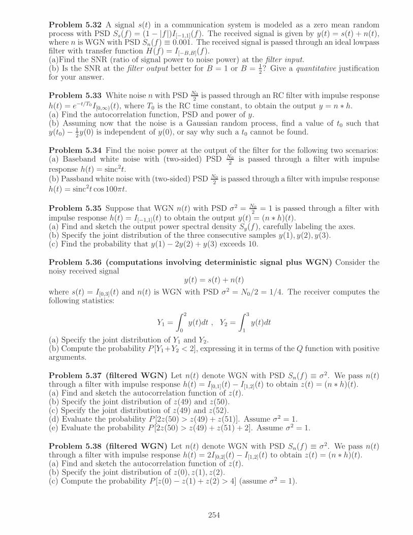
Problem 5.32 A signal s(t) in a communication system is modeled as a zero mean randomprocess with PSD Ss(f) = (1 − |f |)I[−1,1](f). The received signal is given by y(t) = s(t) + n(t),where n is WGN with PSD Sn(f) ≡ 0.001. The received signal is passed through an ideal lowpassfilter with transfer function H(f) = I[−B,B](f).(a)Find the SNR (ratio of signal power to noise power) at the filter input.(b) Is the SNR at the filter output better for B = 1 or B = 1

2? Give a quantitative justification

for your answer.

Problem 5.33 White noise n with PSD N0

2is passed through an RC filter with impulse response

h(t) = e−t/T0I[0,∞)(t), where T0 is the RC time constant, to obtain the output y = n ∗ h.(a) Find the autocorrelation function, PSD and power of y.(b) Assuming now that the noise is a Gaussian random process, find a value of t0 such thaty(t0)− 1

2y(0) is independent of y(0), or say why such a t0 cannot be found.

Problem 5.34 Find the noise power at the output of the filter for the following two scenarios:(a) Baseband white noise with (two-sided) PSD N0

2is passed through a filter with impulse

response h(t) = sinc2t.(b) Passband white noise with (two-sided) PSD N0

2is passed through a filter with impulse response

h(t) = sinc2t cos 100πt.

Problem 5.35 Suppose that WGN n(t) with PSD σ2 = N0

2= 1 is passed through a filter with

impulse response h(t) = I[−1,1](t) to obtain the output y(t) = (n ∗ h)(t).(a) Find and sketch the output power spectral density Sy(f), carefully labeling the axes.(b) Specify the joint distribution of the three consecutive samples y(1), y(2), y(3).(c) Find the probability that y(1)− 2y(2) + y(3) exceeds 10.

Problem 5.36 (computations involving deterministic signal plus WGN) Consider thenoisy received signal

y(t) = s(t) + n(t)

where s(t) = I[0,3](t) and n(t) is WGN with PSD σ2 = N0/2 = 1/4. The receiver computes thefollowing statistics:

Y1 =

∫ 2

0

y(t)dt , Y2 =

∫ 3

1

y(t)dt

(a) Specify the joint distribution of Y1 and Y2.(b) Compute the probability P [Y1+Y2 < 2], expressing it in terms of the Q function with positivearguments.

Problem 5.37 (filtered WGN) Let n(t) denote WGN with PSD Sn(f) ≡ σ2. We pass n(t)through a filter with impulse response h(t) = I[0,1](t)− I[1,2](t) to obtain z(t) = (n ∗ h)(t).(a) Find and sketch the autocorrelation function of z(t).(b) Specify the joint distribution of z(49) and z(50).(c) Specify the joint distribution of z(49) and z(52).(d) Evaluate the probability P [2z(50) > z(49) + z(51)]. Assume σ2 = 1.(e) Evaluate the probability P [2z(50) > z(49) + z(51) + 2]. Assume σ2 = 1.

Problem 5.38 (filtered WGN) Let n(t) denote WGN with PSD Sn(f) ≡ σ2. We pass n(t)through a filter with impulse response h(t) = 2I[0,2](t)− I[1,2](t) to obtain z(t) = (n ∗ h)(t).(a) Find and sketch the autocorrelation function of z(t).(b) Specify the joint distribution of z(0), z(1), z(2).(c) Compute the probability P [z(0)− z(1) + z(2) > 4] (assume σ2 = 1).

254

Problem 5.39 (filtered and sampled WGN) Let n(t) denote WGN with PSD Sn(f) ≡ σ2.We pass n(t) through a filter with impulse response h(t) to obtain z(t) = (n ∗ h)(t), and thensample it at rate 1/Ts to obtain the sequence z[n] = z(nTs), where n takes integer values.(a) Show that

cov(z[n], z[m]) = E[z[n]z∗[m]] =N0

2

∫

h(t)h∗(t− (n−m)Ts)

(We are interested in real-valued impulse responses, but we continue to develop a frameworkgeneral enough to encompass complex-valued responses.)(b) For h(t) = I[0,1](t), specify the joint distribution of (z[1], z[2], z[3])T for a sampling rate of 2(Ts =

12).

(c) Repeat (b) for a sampling rate of 1.(d) For a general h sampled at rate 1/Ts, show that the noise samples are independent if h(t) issquare root Nyquist at rate 1/Ts.

Problem 5.40 Consider the signal s(t) = I[0,2](t)− 2I[1,3](t).(a) Find and sketch the impulse response smf(t) of the matched filter for s.(b) Find and sketch the output when s(t) is passed through its matched filter.(c) Suppose that, instead of the matched filter, all we have available is a filter with impulseresponse h(t) = I[0,1](t). For an arbitrary input signal x(t), show how z(t) = (x ∗ smf )(t) can besynthesized from y(t) = (x ∗ h)(t).

Problem 5.41 (Correlation via filtering and sampling) A signal x(t) is passed through afilter with impulse response h(t) = I[0,2](t) to obtain an output y(t) = (x ∗ h)(t).(a) Find and sketch a signal g1(t) such that

y(2) = 〈x, g1〉 =∫

x(t)g1(t)dt

(b) Find and sketch a signal g2(t) such that

y(1)− 2y(1) = 〈x, g2〉 =∫

x(t)g2(t)dt

Problem 5.42 (Correlation via filtering and sampling) Let us generalize the result wewere hinting at in Problem 5.41. Suppose an arbitrary signal x is passed through an arbitraryfilter h(t) to obtain output y(t) = (x ∗ h)(t).(a) Show that taking a linear combination of samples at the filter output is equivalent to acorrelation operation on u. That is, show that

n∑

i=1

αiy(ti) = 〈x, g〉 =∫

x(t)g(t)dt

where

g(t) =

n∑

i=1

αih(ti − t) =

n∑

i=1

αihmf (t− ti) (5.108)

That is, taking a linear combination of samples is equivalent to correlating against a signal whichis a linear combination of shifted versions of the matched filter for h.(b) The preceding result can be applied to approximate a correlation operation by taking linearcombinations at the output of a filter. Suppose that we wish to perform a correlation against atriangular pulse g(t) = (1− |t|)I[−1,1](t). How would you approximate this operation by taking alinear combination of samples at the output of a filter with impulse response h(t) = I[0,1](t).

255

Problem 5.43 (Approximating a correlator by filtering and sampling) Consider thenoisy signal

y(t) = s(t) + n(t)

where s(t) = (1− |t|)I[−1,1](t), and n(t) is white noise with Sn(f) ≡ 0.1.(a) Compute the SNR at the output of the integrator

Z =

∫ 1

−1

y(t)dt

(b) Can you improve the SNR by modifying the integration in (a), while keeping the processinglinear? If so, say how. If not, say why not.(c) Now, suppose that y(t) is passed through a filter with impulse response h(t) = I[0,1](t) toobtain z(t) = (y ∗ h)(t). If you were to sample the filter output at a single time t = t0, howwould you choose t0 so as to maximize the SNR?(d) In the setting of (c), if you were now allowed to take two samples at times t1, t2 and t3 andgenerate a linear combination a1z(t1) + a2z(t2) + a3z(t3), how would you choose ai, ti, toimprove the SNR relative to (c). (We are looking for intuitively sensible answers rather than aprovably optimal choice.)Hint: See Problem 5.42. Taking linear combinations of samples at the output of a filter isequivalent to correlation with an appropriate waveform, which we can choose to approximate theoptimal correlator.

Mathematical derivations

Problem 5.44 (Bounds on the Q function) We derive the bounds (5.117) and (5.116) for

Q(x) =

∫ ∞

x

1√2πe−t2/2dt (5.109)

(a) Show that, for x ≥ 0, the following upper bound holds:

Q(x) ≤ 1

2e−x2/2

Hint: Try pulling out a factor of e−x2from (5.109), and then bounding the resulting integrand.

Observe that t ≥ x ≥ 0 in the integration interval.(b) For x ≥ 0, derive the following upper and lower bounds for the Q function:

(1− 1

x2)e−x2/2

√2πx

≤ Q(x) ≤ e−x2/2

√2πx

Hint: Write the integrand in (5.109) as a product of 1/t and te−t2/2 and then integrate by partsto get the upper bound. Integrate by parts once more using a similar trick to get the lowerbound. Note that you can keep integrating by parts to get increasingly refined upper and lowerbounds.

Problem 5.45 (Geometric derivation of Q function bound) Let X1 and X2 denote inde-pendent standard Gaussian random variables.(a) For a > 0, express P [|X1| > a, |X2| > a] in terms of the Q function.(b) Find P [X2

1 +X22 > 2a2].

Hint: Transform to polar coordinates. Or use the results of Problem 5.21.(c) Sketch the regions in the (x1, x2) plane corresponding to the events considered in (a) and (b).

(d) Use (a)-(c) to obtain an alternative derivation of the bound Q(x) ≤ 12e−x2/2 for x ≥ 0 (i.e.,

the bound in Problem 5.44(a)).

256

Problem 5.46 (Cauchy-Schwartz inequality for random variables) For random variablesX and Y defined on a common probability space, define the mean squared error in approximatingX by a multiple of Y as

J(a) = E[

(X − aY )2]

where a is a scalar. Assume that both random variables are nontrivial (i.e., neither of them iszero with probability one).(a) Show that

J(a) = E[X2] + a2E[Y 2]− 2aE[XY ]

(b) Since J(a) is quadratic in a, it has a global minimum (corresponding to the best approxima-

tion of X by a multiple of Y ). Show that this is achieved for aopt =E[XY ]E[Y 2]

.

(c) Show that the mean squared error in the best approximation found in (b) can be written as

J(aopt) = E[X2]− (E[XY ])2

E[Y 2]

(d) Since the approximation error is nonnegative, conclude that

(E[XY ])2 ≤ E[X2]E[Y 2] Cauchy − Schwartz inequality for random variables (5.110)

This is the Cauchy-Schwartz inequality for random variables.(e) Conclude also that equality is achieved in (5.110) if and only if X and Y are scalar multiplesof each other.Hint: Equality corresponds to J(aopt) = 0.

Problem 5.47 (Normalized correlation) (a) Apply the Cauchy-Schwartz inequality in theprevious problem to “zero mean” versions of the random variables, X1 = X−E[X ], Y1 = Y −E[Y ]to obtain that

|cov(X, Y )| ≤√

var(X)var(Y ) (5.111)

(b) Conclude that the normalized correlation ρ(X, Y ) defined in (5.59) lies in [−1, 1].(c) Show that |ρ| = 1 if and only if we can write X = aY + b. Specify the constants a and b interms of the means and covariances associated with the two random variables.

Problem 5.48 (Characteristic function of a Gaussian random vector) Consider a Gaus-sian random vector X = (X1, ..., Xm)

T ∼ N(m,C). The characteristic function of X is definedas follows:

φX(w) = E

[

ejwTX]

= E[

ej(w1X1+...+wmXm)]

(5.112)

The characteristic function completely characterizes the distribution of a random vector, even if adensity does not exist. If the density does exist, the characteristic function is a multidimensionalinverse Fourier transform of it:

φX(w) = E

[

ejwTX]

=

∫

ejwTXpX(x) dx

The density is therefore given by the corresponding Fourier transform

pX(x) =1

(2π)m

∫

e−jwTxφX(w) dw (5.113)

(a) Show that Y = wTX is a Gaussian random variable with mean µ = wTm and variancev2 = wTCw.(b) For Y ∼ N(µ, v2), show that

E[ejY ] = ejµ−v2

2

257

(c) Use the result of (b) to obtain that the characteristic function of X is given by

φX(w) = ejwTm− 1

2wTCw (5.114)

which depends only on m and C.(d) Since the distribution ofX is completely specified by its characteristic function, conclude thatthe distribution of a Gaussian random vector depends only on its mean vector and covariancematrix. When C is invertible, we can compute the density (5.58) by taking the Fourier transformof the characteristic funciton in (5.114), but we skip that derivation.

Problem 5.49 Consider a zero mean WSS random process X with autocorrelation functionRX(τ). Let Y1(t) = (X ∗ h1)(t) and Y2(t) = (X ∗ h2)(t) denote random processes obtained bypassing X through LTI systems with impulse responses h1 and h2, respectively.(a) Find the crosscorrelation function RY1,Y2(t1, t2).Hint: You can use the approach employed to obtain (5.101), first finding RY1,X and then RY1,Y2.(b) Are Y1 and Y2 jointly WSS?(c) Suppose that X is white noise with PSD SX(f) ≡ 1, h1(t) = I[0,1](t) and h2(t) = e−tI[0,∞)(t).Find E[Y1(0)Y2(0)] and E[Y1(0)Y2(1)].

Problem 5.50 (Cauchy-Schwartz inequality for signals) Consider two signals (assumereal-valued for simplicity, although the results we are about to derive apply for complex-valuedsignals as well) u(t) and v(t).(a) We wish to approximate u(t) by a scalar multiple of v(t) so as to minimize the norm of theerror. Specifically, we wish to minimize

J(a) =

∫

|u(t)− av(t)|2dt = ||u− av||2 = 〈u− av, u− av〉

Show thatJ(a) = ||u||2 + a2||v||2 − 2a〈u, v〉

(b) Show that the quadratic function J(a) is minimized by choosing a = aopt, given by

aopt =〈u, v〉||v||2

Show that the corresponding approximation aoptv can be written as a projection of u along aunit vector in the direction of v:

aoptv = 〈u, v

||v||〉v

||v||(c) Show that the error due to the optimal setting is given by

J(aopt) = ||u||2 − |〈u, v〉|2||v||2

(d) Since the minimum error is non-negative, conclude that

||u||||v|| ≤ |〈u, v〉| , Cauchy − Schwartz inequality for signals (5.115)

This is the Cauchy-Schwartz inequality, which applies to real- and complex-valued signals orvectors.(e) Conclude also that equality in (5.115) occurs if and only if u is a scalar multiple of v or if vis a scalar multiple of u. (We need to say it both ways in case one of the signals is zero.)

258

Problem 5.51 Consider a random process X passed through a correlator g to obtain

Z =

∫ ∞

−∞X(t)g(t)dt

where X(t), g(t) are real-valued.(a) Show that the mean and variance of Z can be expressed in terms of the mean function andautovariance function) of X as follows:

E[Z] =

∫

mX(t)g(t)dt = 〈mX , g〉

var(Z) =

∫ ∫

CX(t1, t2)g(t1)g(t2)dt1dt2

(b) Suppose now that X is zero mean and WSS with autocorrelation RX(τ). Show that thevariance of the correlator output can be written as

var(Z) =

∫

RX(τ)Rg(τ) dτ = 〈RX , Rg〉

where Rg(τ) = (g ∗ gMF )(τ) =∫

g(t)g(t− τ) dt is the “autocorrelation” of the waveform g.Hint: An alternative to doing this from scratch is to use the equivalence of correlation andmatched filtering. You can then employ (5.101), which gives the output autocorrelation functionwhen a WSS process is sent through an LTI system, evaluate it at zero lag to find the power,and use the symmetry of autocorrelation functions.

Problems drawing on material from Chapter 3 and Appendix 5.E

These can be skipped by readers primarily interested in the digital communication material in thesucceeding chapters.

Problem 5.52 Consider a noisy FM signal of the form

v(t) = 20 cos(2πfct+ φs(t)) + n(t)

where n(t) is WGN with power spectral density N0

2= 10−5, and φs(t) is the instantaneous phase

deviation of the noiseless FM signal. Assume that the bandwidth of the noiseless FM signal is100 KHz.(a) The noisy signal v(t) is passed through an ideal BPF which exactly spans the 100 KHzfrequency band occupied by the noiseless signal. What is the SNR at the output of the BPF?(b) The output of the BPF is passed through an ideal phase detector, followed by a differentiatorwhich is normalized to give unity gain at 10 KHz, and an ideal (unity gain) LPF of bandwidth10 KHz.(i) Sketch the noise PSD at the output of the differentiator.(ii) Find the noise power at the output of the LPF.

Problem 5.53 An FM signal of bandwidth 210 KHz is received at a power of -90 dBm, and iscorrupted by bandpass AWGN with two-sided PSD 10−22 watts/Hz. The message bandwidth is5 KHz, and the peak-to-average power ratio for the message is 10 dB.(a) What is the SNR (in dB) for the received FM signal? (Assume that the noise is bandlimitedto the band occupied by the FM signal.)(b) Estimate the peak frequency deviation.(c) The noisy FM signal is passed through an ideal phase detector. Estimate and sketch thenoise PSD at the output of the phase detector, carefully labeling the axes.(d) The output of the phase detector is passed through a differentiator with transfer functionH(f) = jf , and then an ideal lowpass filter of bandwidth 5 kHz. Estimate the SNR (in dB) atthe output of the lowpass filter.

259

Problem 5.54 A message signal m(t) is modeled as a zero mean random process with PSD

Sm(f) = |f |I[−2,2](f)

We generate an SSB signal as follows:

u(t) = 20[m(t) cos 200πt− m(t) sin 200πt]

where m denotes the Hilbert transform of m.(a) Find the power of m and the power of u.(b) The noisy received signal is given by y(t) = u(t)+n(t), where n is passband AWGN with PSDN0

2= 1, and is independent of u. Draw the block diagram for an ideal synchronous demodulator

for extracting the message m from y, specifying the carrier frequency as well as the bandwidthof the LPF, and find the SNR at the output of the demodulator.(c) Find the signal-to-noise-plus-interference ratio if the local carrier for the synchronous demod-ulator has a phase error of π

8.

5.A Q function bounds and asymptotics

The following upper and lower bounds on Q(x) (derived in Problem 5.44) are asymptoticallytight for large arguments; that is, the difference between the bounds tends to zero as x getslarge.

Bounds on Q(x), asymptotically tight for large arguments

(

1− 1

x2

)

e−x2/2

x√2π

≤ Q(x) ≤ e−x2/2

x√2π

, x ≥ 0 (5.116)

The asymptotic behavior (5.53) follows from these bounds. However, they do not work well forsmall x (the upper bound blows up to ∞, and the lower bound to −∞, as x→ 0). The followingupper bound is useful for both small and large values of x ≥ 0: it gives accurate results for smallx, and, while it is not as tight as the bounds (5.116) for large x, it does give the correct exponentof decay.

Upper bound on Q(x) useful for both small and large arguments

Q(x) ≤ 1

2e−x2/2 , x ≥ 0 (5.117)

Figure 5.29 plots Q(x) and its bounds for positive x. A logarithmic scale is used for the valuesof the function in order to demonstrate the rapid decay with x. The bounds (5.116) are seen tobe tight even at moderate values of x (say x ≥ 2), while the bound (5.117) shows the right rateof decay for large x, while also remaining useful for small x.

5.B Approximations using Limit Theorems

We often deal with sums of independent (or approximately independent) random variables. Find-ing the exact distribution of such sums can be cumbersome. This is where limit theorems, whichcharacterize what happens to these sums as the number of terms gets large, come in handy.

Law of large numbers (LLN): Suppose that X1, X2, ... are i.i.d. random variables with finitemean m. Then their empirical average (X1 + ... + Xn)/n converges to their statistical average

260

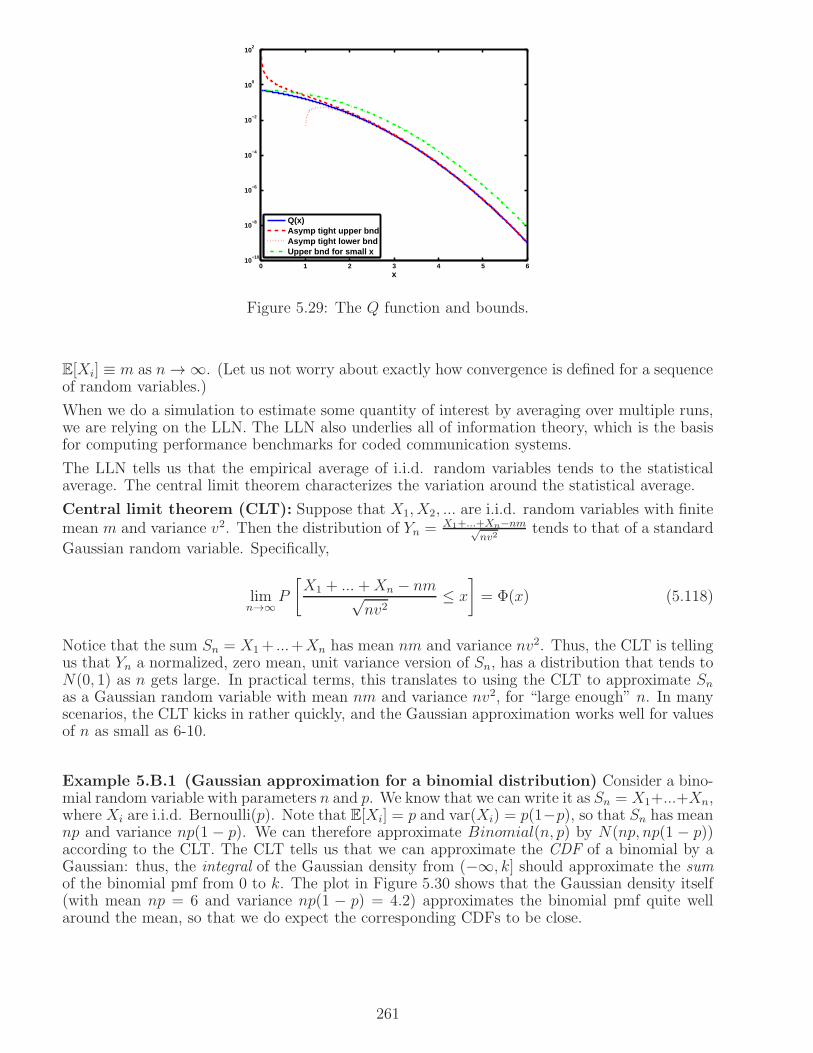
0 1 2 3 4 5 610

−10

10−8

10−6

10−4

10−2

100

102

x

Q(x)Asymp tight upper bndAsymp tight lower bndUpper bnd for small x

Figure 5.29: The Q function and bounds.

E[Xi] ≡ m as n→ ∞. (Let us not worry about exactly how convergence is defined for a sequenceof random variables.)

When we do a simulation to estimate some quantity of interest by averaging over multiple runs,we are relying on the LLN. The LLN also underlies all of information theory, which is the basisfor computing performance benchmarks for coded communication systems.

The LLN tells us that the empirical average of i.i.d. random variables tends to the statisticalaverage. The central limit theorem characterizes the variation around the statistical average.

Central limit theorem (CLT): Suppose that X1, X2, ... are i.i.d. random variables with finitemean m and variance v2. Then the distribution of Yn = X1+...+Xn−nm√

nv2tends to that of a standard

Gaussian random variable. Specifically,

limn→∞

P

[

X1 + ... +Xn − nm√nv2

≤ x

]

= Φ(x) (5.118)

Notice that the sum Sn = X1+ ...+Xn has mean nm and variance nv2. Thus, the CLT is tellingus that Yn a normalized, zero mean, unit variance version of Sn, has a distribution that tends toN(0, 1) as n gets large. In practical terms, this translates to using the CLT to approximate Sn

as a Gaussian random variable with mean nm and variance nv2, for “large enough” n. In manyscenarios, the CLT kicks in rather quickly, and the Gaussian approximation works well for valuesof n as small as 6-10.

Example 5.B.1 (Gaussian approximation for a binomial distribution) Consider a bino-mial random variable with parameters n and p. We know that we can write it as Sn = X1+...+Xn,where Xi are i.i.d. Bernoulli(p). Note that E[Xi] = p and var(Xi) = p(1−p), so that Sn has meannp and variance np(1 − p). We can therefore approximate Binomial(n, p) by N(np, np(1 − p))according to the CLT. The CLT tells us that we can approximate the CDF of a binomial by aGaussian: thus, the integral of the Gaussian density from (−∞, k] should approximate the sumof the binomial pmf from 0 to k. The plot in Figure 5.30 shows that the Gaussian density itself(with mean np = 6 and variance np(1 − p) = 4.2) approximates the binomial pmf quite wellaround the mean, so that we do expect the corresponding CDFs to be close.

261

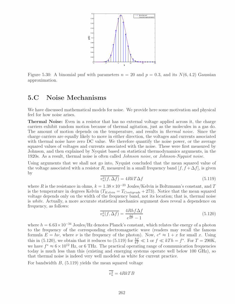
−5 0 5 10 15 200

0.02

0.04

0.06

0.08

0.1

0.12

0.14

0.16

0.18

0.2

k

p(k)

Binomial pmfGaussian approximation

Figure 5.30: A binomial pmf with parameters n = 20 and p = 0.3, and its N(6, 4.2) Gaussianapproximation.

5.C Noise Mechanisms

We have discussed mathematical models for noise. We provide here some motivation and physicalfeel for how noise arises.

Thermal Noise: Even in a resistor that has no external voltage applied across it, the chargecarriers exhibit random motion because of thermal agitation, just as the molecules in a gas do.The amount of motion depends on the temperature, and results in thermal noise. Since thecharge carriers are equally likely to move in either direction, the voltages and currents associatedwith thermal noise have zero DC value. We therefore quantify the noise power, or the averagesquared values of voltages and currents associated with the noise. These were first measured byJohnson, and then explained by Nyquist based on statistical thermodynamics arguments, in the1920s. As a result, thermal noise is often called Johnson noise, or Johnson-Nyquist noise.

Using arguments that we shall not go into, Nyquist concluded that the mean squared value ofthe voltage associated with a resistor R, measured in a small frequency band [f, f +∆f ], is givenby

v2n(f,∆f) = 4RkT∆f (5.119)

where R is the resistance in ohms, k = 1.38×10−23 Joules/Kelvin is Boltzmann’s constant, and Tis the temperature in degrees Kelvin (TKelvin = TCentigrade +273). Notice that the mean squaredvoltage depends only on the width of the frequency band, not its location; that is, thermal noiseis white. Actually, a more accurate statistical mechanics argument does reveal a dependence onfrequency, as follows:

v2n(f,∆f) =4Rhf∆f

ehfkT − 1

(5.120)

where h = 6.63×10−34 Joules/Hz denotes Planck’s constant, which relates the energy of a photonto the frequency of the corresponding electromagnetic wave (readers may recall the famousformula E = hν, where ν is the frequency of the photon). Now, ex ≈ 1 + x for small x. Usingthis in (5.120), we obtain that it reduces to (5.119) for hf

kT≪ 1 or f ≪ kTh = f ∗. For T = 290K,

we have f ∗ ≈ 6×1012 Hz, or 6 THz. The practical operating range of communication frequenciestoday is much less than this (existing and emerging systems operate well below 100 GHz), sothat thermal noise is indeed very well modeled as white for current practice.

For bandwidth B, (5.119) yields the mean squared voltage

v2n = 4RkTB

262

Now, if we connect the noise source to a matched load of impedance R, the mean squared powerdelivered to the load is

P 2n =

(vn/2)2

R= kTB (5.121)

The preceding calculation provides a valuable benchmark, giving the communication link designera ballpark estimate of how much noise power to expect in a receiver operating over a bandwidth B.Of course, the noise for a particular receiver is typically higher than this benchmark, and must becalculated based on detailed modeling and simulation of internal and external noise sources, andthe gains, input impedances, and output impedances for various circuit components. However,while the circuit designer must worry about these details, once the design is complete, he or shecan supply the link designer with a single number for the noise power at the receiver output,referred to the benchmark (5.121).

Shot noise: Shot noise occurs because of the discrete nature of the charge carriers. When avoltage applied across a device causes current to flow, if we could count the number of chargecarriers going from one point in the device to the other (e.g., from the source to the drain ofa transistor) over a time period τ , we would see a random number N(τ), which would varyindependently across disjoint time periods. Under rather general assumptions, N(τ) is wellmodeled as a Poisson random variable with mean λτ , where λ scales with the DC current. Thevariance of a Poisson random variable equals its mean, so that the variance of the rate of chargecarrier flow equals

var(N(τ)

τ) =

1

τ 2var(N(τ)) =

λ

τ

We can think of this as the power of the shot noise. Thus, increasing the observation intervalτ smooths out the variations in charge carrier flow, and reduces the shot noise power. If wenow think of the device being operated over a bandwidth B, we know that we are effectivelyobserving the device at a temporal resolution τ ∼ 1

B. Thus, shot noise power scales linearly with

B.

The preceding discussion indicates that both thermal noise and shot noise are white, in thattheir power scales linearly with the system bandwidth B, independent of the frequency band ofoperation. We can therefore model the aggregate system noise due to these two phenomena as asingle white noise process. Indeed, both phenomena involve random motions of a large numberof charge carriers, and can be analyzed together in a statistical mechanics framework. This iswell beyond our scope, but for our purpose, we can simply model the aggregate system noise dueto these phenomena as a single white noise process.

Flicker noise: Another commonly encountered form of noise is 1/f noise, also called flickernoise, whose power increases as the frequency of operation gets smaller. The sources of 1/fnoise are poorly understood, and white noise dominates in the typical operating regimes forcommunication receivers. For example, in an RF system, the noise in the front end (antenna,low noise amplifier, mixer) dominates the overall system noise, and 1/f noise is negligible atthese frequencies. We therefore ignore 1/f noise in our noise modeling.

5.D The structure of passband random processes

We discuss here the modeling of passband random processes, and in particular, passband whitenoise, in more detail. These insights are useful for the analysis of the effect of noise in analogcommunication systems, as in Appendix 5.E.

We can define the complex envelope, and I and Q components, for a passband random processin exactly the same fashion as is done for deterministic signals in Chapter 2. For a passbandrandom process, each sample path (observed over a large enough time window) has a Fourier

263

transform restricted to passband. We can therefore define complex envelope, I/Q componentsand envelope/phase as we do for deterministic signals. For any given reference frequency fc inthe band of interest, any sample path xp(t) for a passband random process can be written as

xp(t) = Re(

x(t)ej2πfct)

xp(t) = xc(t) cos 2πfct− xs(t) sin 2πfctxp(t) = e(t) cos (2πfct+ θ(t))

where x(t) = xc(t) + jxs(t) = e(t)ejθ(t) is the complex envelope, xc(t), xs(t) are the I and Qcomponents, respectively, and e(t), θ(t) are the envelope and phase, respectively.

PSD of complex envelope: Applying the standard frequency domain relationship to thetime-windowed sample paths, we have the frequency domain relationship

Xp,To(f) =1

2XTo(f − fc) +

1

2X∗

To(−f − fc)

We therefore

|Xp,To(f)|2 =1

4|XTo(f − fc)|2 +

1

4|X∗

To(−f − fc)|2 =

1

4|XTo(f − fc)|2 +

1

4|XTo(−f − fc)|2

Dividing by To and letting To → ∞, we obtain

Sxp(f) =1

4Sx(f − fc) +

1

4Sx(−f − fc) (5.122)

where Sx(f) is baseband. Using (5.87), the one-sided passband PSD is given by

S+xp(f) =

1

2Sx(f − fc) (5.123)

Similarly, we can go from passband to complex baseband using the formula

Sx(f) = 2S+xp(f + fc) (5.124)

What about the I and Q components? Consider the complex envelope x(t) = xc(t) + jxs(t). Itsautocorrelation function is given by

Rx(τ) = x(t)x∗(t− τ) = (xc(t) + jxs(t)) (xc(t− τ)− jxs(t− τ))

which yieldsRx(τ) = (Rxc(τ) +Rxs(τ)) + j (Rxs,xc(τ)− Rxc,xs(τ))

= (Rxc(τ) +Rxs(τ)) + j (Rxs,xc(τ)− Rxs,xc(−τ))(5.125)

Taking the Fourier transform, we obtain

Sx(f) = Sxc(f) + Sxs(f) + j(

Sxs,xc(f)− S∗xs,xc

(f))

which simplifies toSx(f) = Sxc(f) + Sxs(f)− 2Im (Sxs,xc(f)) (5.126)

For simplicity, we henceforth consider situations in which Sxs,xc(f) ≡ 0 (i.e., the I and Q com-ponents are uncorrelated). Actually, for a given passband random process, even if the I andQ components for a given frequency reference are uncorrelated, we can make them correlatedby shifting the frequency reference. However, such subtleties are not required for our purpose,which is to model digitally modulated signals and receiver noise.

264

5.D.1 Baseband representation of passband white noise

Consider passband white noise as shown in Figure 5.21. If we choose the reference frequency asthe center of the band, then we get a simple model for the complex envelope and the I and Qcomponents of the noise, as depicted in Figure 5.31. The complex envelope has PSD

Sn(f) = 2N0 , |f | ≤ B/2

and the I and Q components have PSDs and cross-spectrum given by

Snc(f) = Sns(f) = N0 , |f | ≤ B/2Sns,nc(f) ≡ 0

B/2

0

nS (f)

0N

cnS (f)snS (f)

−B/2f

PSD of I and Q components PSD of complex envelope

−B/2

=

fB/2

2 N

Figure 5.31: PSD of I and Q components, and complex envelope, of passband white noise.

Note that the power of the complex envelope is 2N0B, which is twice the power of the correspond-ing passband noise np. This is consistent with the convention in Chapter 2 for deterministic,finite-energy signals, where the complex envelope has twice the energy of the corresponding pass-band signal. Later, when we discuss digital communication receivers and their performance inChapter 6, we find it convenient to scale signals and noise in complex baseband such that we getrid of this factor of two. In this case, we obtain that the PSD of the I and Q components PSDsare given by Snc(f) = Sns(f) = N0/2.

Passband White Noise is Circularly Symmetric

LowpassFilter

2cos(2 f t− )π c θ

pn (t) n (t)b

Figure 5.32: Circular symmetry implies that the PSD of the baseband noise nb(t) is independentof θ.

An important property of passband white noise is its circular symmetry: the statistics of the Iand Q components are unchanged if we change the phase reference. To understand what thismeans in practical terms, consider the downconversion operation shown in Figure 5.32, which

265

yields a baseband random process nb(t). Circular symmetry corresponds to the assumption thatthe PSD of nb does not depend on θ. Thus, it immediately implies that

Snc(f) = Sns(f) ↔ Rnc(τ) = Rns(τ) (5.127)

since nb = nc for θ = 0, and nb = ns. for θ = −π2, where nc, ns are the I and Q components,

respectively, taking fc = f0 as a reference. Thus, changes in phase reference do not change thestatistics of the I and Q components.

5.E SNR Computations for Analog Modulation

We now compute SNR for the amplitude and angle modulation schemes discussed in Chapter 3.Since the format of the messages is not restricted in our analysis, the SNR computations applyto digital modulation (where the messages are analog waveforms associated with a particularsequence of bits being transmitted) as well as analog modulation (where the messages are typically“natural” audio or video waveforms beyond our control). However, such SNR computations areprimarily of interest for analog modulation, since the performance measure of interest for digitalcommunication systems is typically probability of error.

5.E.1 Noise Model and SNR Benchmark

For noise modeling, we consider passband, circularly symmetric, white noise np(t) in a systemof bandwidth B centered around fc, with PSD as shown in Figure 5.21. As discussed in Section5.D.1, we can write this in terms of its I and Q components with respect to reference frequencyfc as

np(t) = nc(t) cos 2πfct− ns(t) sin 2πfct

where the relevant PSDs are given in Figure 5.31.

Baseband benchmark: When evaluating the SNR for various passband analog modulationschemes, it is useful to consider a hypothetical baseband system as benchmark. Suppose thata real-valued message of bandwidth Bm is sent over a baseband channel. The noise power overthe baseband channel is given by Pn = N0Bm. If the received signal power is Pr = Pm, then theSNR benchmark for this baseband channel is given by:

SNRb =Pr

N0Bm(5.128)

5.E.2 SNR for Amplitude Modulation

We now quickly sketch SNR computations for some of the variants of AM. The signal and powercomputations are similar to earlier examples in this chapter, so we do not belabor the details.

SNR for DSB-SC: For message bandwidth Bm, the bandwidth of the passband received signalis B = 2Bm. The received signal given by

yp(t) = Acm(t) cos(2πfct+ θr) + np(t)

where θr is the phase offset between the incoming carrier and the LO. The received signal poweris given by

Pr = (Acm(t) cos(2πfct+ θr))2 = A2

cPm/2

266

A coherent demodulator extracts the I component, which is given by

yc(t) = Acm(t) cos θr + nc(t)

The signal power is

Ps = (Acm(t) cos θr)2 = A2

cPm cos2 θr

while the noise power isPn = n2

c(t) = N0B = 2N0Bm

so that the SNR is

SNRDSB =A2

cPm cos2 θr2N0Bm

=Pr

N0Bmcos2 θr = SNRb cos

2 θr (5.129)

which is the same as the baseband benchmark (5.128) For ideal coherent demodulation (i.e.,θr = 0), we obtain that the SNR for DSB equals the baseband benchmark SNRb in (5.128).

SNR for SSB: For message bandwidth Bm, the bandwidth of the passband received signal isB = Bm. The received signal given by

yp(t) = Acm(t) cos(2πfct+ θr)± Acm(t) sin(2πfct+ θr) + np(t)

where θr is the phase offset between the incoming carrier and the LO. The received signal poweris given by

Pr = (Acm(t) cos(2πfct+ θr))2 + (Acm(t) sin(2πfct+ θr))

2 = A2cPm

A coherent demodulator extracts the I component, which is given by

yc(t) = Acm(t) cos θr ∓ Acm(t) sin θr + nc(t)

The signal power is

Ps = (Acm(t) cos θr)2 = A2

cPm cos2 θr

while the noise plus interference power is

Pn = n2c(t) + (Acm(t) sin θr)2 = N0B + A2

cPm sin2 θr = N0Bm + A2cPm sin2 θr

so that the signal-to-interference-plus-noise (SINR) is

SINRSSB = A2cPm cos2 θr

N0Bm+A2cPm sin2 θr

= Pr cos2 θrN0Bm+Pr sin2 θr

= SNRb cos2 θr

1+SNRb sin2 θr

(5.130)

This coincides with the baseband benchmark (5.128) for ideal coherent demodulation (i.e., θr =0). However, for θr 6= 0, even when the received signal power Pr gets arbitrarily large relative tothe noise power, the SINR cannot be larger than 1

tan2 θr, which shows the importance of making

the phase error as small as possible.

SNR for AM: Now, consider conventional AM. While we would typically use envelope detectionrather than coherent demodulation in this setting, it is instructive to compute SNR for bothmethods of demodulation. For message bandwidth Bm, the bandwidth of the passband receivedsignal is B = 2Bm. The received signal given by

yp(t) = Ac (1 + amodmn(t)) cos(2πfct+ θr) + np(t) (5.131)

267

where mn(t) is the normalized version of the message (with mintmn(t) = −1), and where θr isthe phase offset between the incoming carrier and the LO. The received signal power is given by

Pr = (Acm(t) cos(2πfct+ θr))2 = A2

c(1 + a2modPmn)/2 (5.132)

where Pmn = m2n(t) is the power of the normalized message. A coherent demodulator extracts

the I component, which is given by

yc(t) = Ac + Acamodmn(t) cos θr + nc(t)

The power of the information-bearing part of the signal (the DC term due to the carrier carriesno information, and is typically rejected using AC coupling) is given by

Ps = (Acamodmn(t) cos θr)2 = A2

ca2modPmn cos

2 θr (5.133)

Recall that the AM power efficiency is defined as the power of the message-bearing part of thesignal to the power of the overall signal (which includes an unmodulated carrier), and is givenby

ηAM =a2modPmn

1 + a2modPmn

We can therefore write the signal power (5.133) at the output of the coherent demodulator interms of the received power in (5.132) as:

Ps = 2PrηAM cos2 θr

while the noise power is

Pn = n2c(t) = N0B = 2N0Bm

Thus, the SNR is

SNRAM,coh = Ps

Pn= 2PrηAM cos2 θr

2N0Bm= SNRbηAM cos2 θr (5.134)

Thus, even with ideal coherent demodulation (θr = 0), the SNR obtained is AM is less than thatof the baseband benchmark, since ηAM < 1 (typically much smaller than one). Of course, thereason we incur this power inefficiency is to simplify the receiver, by message recovery using anenvelope detector. Let us now compute the SNR for the latter.

e(t)s

cA (1+a m (t))+ n (t)mod cn = y (t)c

= y (t)s

θr

n (t)

Figure 5.33: At high SNR, the envelope of an AM signal is approximately equal to its I componentrelative to the received carrier phase reference.

Expressing the passband noise in the received signal (5.131) with the incoming carrier as thereference, we have

yp(t) = Ac (1 + amodmn(t)) cos(2πfct+ θr) + nc(t) cos(2πfct + θr)− ns(t) sin(2πfct+ θr)

268

where, by virtue of circular symmetry, nc, ns have the PSDs and cross-spectra as in Figure 5.31,regardless of θr. That is,

yp(t) = yc(t) cos(2πfct+ θr)− ys(t) sin(2πfct + θr)

where, as shown in Figure 5.33,

yc(t) = Ac (1 + amodmn(t)) + nc(t) , ys(t) = ns(t)

At high SNR, the signal term is dominant, so that yc(t) ≫ ys(t). Furthermore, since the AMsignal is positive (assuming amod < 1), so that yc > 0 “most of the time,” even though nc can benegative. We therefore obtain that

e(t) =√

y2c (t) + y2s(t) ≈ |yc(t)| ≈ yc(t)

That is, the output of the envelope detector is approximated, for high SNR, as

e(t) ≈ Ac (1 + amodmn(t)) + nc(t)

The right-hand side is what we would get from ideal coherent detection. We can reuse our SNRcomputation for coherent detection to conclude that the SNR at the envelope detector output isgiven by

SNRAM,envdet = SNRbηAM (5.135)

Thus, for a properly designed (amod < 1) AM system operating at high SNR, the envelopedetector approximates the performance of ideal coherent detection, without requiring carriersynchronization.

5.E.3 SNR for Angle Modulation

We have seen how to compute SNR when white noise adds to a message encoded in the signalamplitude. Let us now see what happens when the message is encoded in the signal phase orfrequency. The received signal is given by

yp(t) = Ac cos(2πfct+ θ(t)) + np(t) (5.136)

where np(t) is passband white noise with one-sided PSD N0 over the signal band of interest, andwhere the message is encoded in the phase θ(t). For example,

θ(t) = kpm(t)

for phase modulation, and1

2π

d

dtθ(t) = kfm(t)

for frequency modulation. We wish to understand how the additive noise np(t) perturbs thephase.

Decomposing the passband noise into I and Q components with respect to the phase of thenoiseless angle modulated signal, we can rewrite the received signal as follows:

yp(t) = Ac cos(2πfct + θ(t)) + nc(t) cos(2πfct+ θ(t))− ns(t) sin(2πfct+ θ(t))= (Ac + nc(t)) cos(2πfct+ θ(t))− ns(t) sin(2πfct+ θ(t))

(5.137)

269

c

θn

(t)θ

n (t)s

A + n (t)c

(t)

Figure 5.34: I and Q components of a noisy angle modulated signal with the phase referencechosen as the phase of the noiseless signal.

where nc, ns have PSDs as in Figure 5.31 (with cross-spectrum Sns,nc(f) ≡ 0), thanks to circularsymmetry (we assume that it applies approximately even though the phase reference θ(t) is time-varying). The I and Q components with respect to this phase reference are shown in Figure 5.34,so that the corresponding complex envelope can be written as

y(t) = e(t)ejθn(t)

where

e(t) =

√

(Ac + nc(t))2 + n2

s(t) (5.138)

and

θn(t) = tan−1 ns(t)

Ac + nc(t)(5.139)

The passband signal in (5.137) can now be rewritten as

yp(t) = Re(y(t)e2πfct+θ(t)) = Re(

e(t)ejθn(t)e2πfct+θ(t))

= e(t) cos (2πfct + θ(t) + θn(t))

At high SNR, Ac ≫ |nc| and Ac ≫ |ns|. Thus,

| ns(t)

Ac + nc(t)| ≪ 1

andns(t)

Ac + nc(t)≈ ns(t)

Ac

For |x| small, tan x ≈ x, and hence x ≈ tan−1 x. We therefore obtain the following high SNRapproximation for the phase perturbation due to the noise:

θn(t) = tan−1 ns(t)

Ac + nc(t)≈ ns(t)

Ac, high SNR approximation (5.140)

To summarize, we can model the received signal (5.136) as

yp(t) ≈ Ac cos(2πfct + θ(t) +ns(t)

Ac) , high SNR approximation (5.141)

Thus, the Q component (relative to the desired signal’s phase reference) of the passband whitenoise appears as phase noise, but is scaled down by the signal amplitude.

270

FM Noise Analysis

Let us apply the preceding to develop an analysis of the effects of white noise on FM. It ishelpful, but not essential, to have read Chapter 3 for this discussion. Suppose that we have anideal detector for the phase of the noisy signal in (5.141), and that we differentiate it to recovera message encoded in the frequency. (For those who have read Chapter 3, we are talking aboutan ideal limiter-discriminator). The output is the instantaneous frequency deviation, given by

z(t) =1

2π

d

dt(θ(t) + θn(t)) ≈ kfm(t) +

n′s(t)

2πAc(5.142)

using the high SNR approximation (5.140).

Estimated

MessageFM Modulator

Channel

RF Frontend

Limiter−Discriminatormessage

Figure 5.35: Block diagram for FM system using limiter-discriminator demodulation.

Before limiter−discriminator

~~~

BRF

N /20

Bm

~~~~

BRFBm

BRF

f N /Ac2

02

fPSD of k m(t)PSD of noiseless FM signal

PSD of passband white noiseNoise PSD

After limiter−discriminator

~

Figure 5.36: PSDs of signal and noise before and after limiter-discriminator.

We now analyze the performance of an FM system whose block diagram is shown in Figure5.35. For wideband FM, the bandwidth BRF of the received signal yp(t) is significantly largerthan the message bandwidth Bm: BRF ≈ 2(β + 1)Bm by Carson’s formula, where β > 1. Thus,the RF front end in Figure 5.35 lets in passband white noise np(t) of bandwidth of the order

271

of BRF , as shown in Figure 5.36. Figure 5.36 also shows the PSDs once we have passed thereceived signal through the limiter-discriminator. The estimated message at the output of thelimiter-discriminator is a baseband signal which we can limit to the message bandwidth Bm,which significantly reduces the noise that we see at the output of the limiter-discriminator. Letus now compute the output SNR. From (5.142), the signal power is given by

Ps = (kfm(t))2 = k2fPm (5.143)

The noise contribution at the output is given by

zn(t) =n′s(t)

2πAc

Since d/dt ↔ j2πf , zn(t) is obtained by passing ns(t) through an LTI system with G(f) =j2πf2πAc

= jf/Ac. Thus, the noise PSD at the output of the limiter-discriminator is given by

Szn(f) = |G(f)|2Sns(f) = f 2N0/A2c , |f | ≤ BRF/2 (5.144)

Once we limit the bandwidth to the message bandwidth Bm after the discriminator, the noisepower is given by

Pn =

∫ Bm

−Bm

Szn(f)df =

∫ Bm

−Bm

f 2N0

A2c

df =2B3

mN0

3A2c

(5.145)

From (5.143) and (5.145), we obtain that the SNR is given by

SNRFM =Ps

Pn=

3k2fPmA2c

2B3mN0

It is interesting to benchmark this against a baseband communication system in which themessage is sent directly over the channel. To keep the comparison fair, we fix the received powerto that of the passband system and the one-sided noise PSD to that of the passband white noise.Thus, the received signal power is Pr = A2

c/2, and the noise power is N0Bm, and the basebandbenchmark SNR is given by

SNRb =Pr

N0Bm=

A2c

2N0Bm

We therefore obtain that

SNRFM =3k2fPm

B2m

SNRb (5.146)

Let us now express this in terms of some interesting parameters. The maximum frequencydeviation in the FM system is given by

∆fmax = kfmaxt|m(t)|

and the modulation index is defined as the ratio between the maximum frequency deviation andthe message bandwidth:

β =∆fmax

Bm

Thus, we havek2fPm

B2m

=(∆fmax)

2

B2m

Pm

(maxt|m(t)|)2= β2/PAR

272

defining the peak-to-average power ratio (PAR) of the message as

PAR =(maxt|m(t)|)2

m2(t)=

(maxt|m(t)|)2Pm

Substituting into (5.146), we obtain that

SNRFM =3β2

PARSNRb (5.147)

Thus, FM can improve upon the baseband benchmark by increasing the modulation index β.This is an example of a power-bandwidth tradeoff: by increasing the bandwidth beyond thatstrictly necessary for sending the message, we have managed to improve the SNR compared to thebaseband benchmark. However, the quadratic power-bandwidth tradeoff offered by FM is highlysuboptimal compared to the best possible tradeoffs in digital communication systems, whereone can achieve exponential tradeoffs. Another drawback of the FM power-bandwidth tradeoffis that the amount of SNR improvement depends on the PAR of the message: messages withlarger dynamic range, and hence larger PAR, will see less improvement. This is in contrast todigital communication, where message characteristics do not affect the power-bandwidth tradeoffsover the communication link, since messages are converted to bits via source coding beforetransmission. Of course, messages with larger dynamic range may well require more bits torepresent them accurately, and hence a higher rate on the communication link, but such designchoices are decoupled from the parameters governing reliable link operation.

Threshold effect: It appears from (5.147) that the output SNR can be improved simply byincreasing β. This is somewhat misleading. For a given message bandwidth Bm, increasing βcorresponds to increasing the RF bandwidth: BRF ≈ 2(β + 1)Bm by Carson’s formula. Thus,an increase in β corresponds to an increase in the power of the the passband white noise atthe input of the limiter-discriminator, which is given by N0BRF = 2N0Bm(β + 1). Thus, if weincrease β, the high SNR approximation underlying (5.140), and hence the model (5.142) for theoutput of the limiter-discriminator, breaks down. It is easy to see this from the equation (5.139)

for the phase perturbation due to noise: θn(t) = tan−1 ns(t)Ac+nc(t)

. When Ac is small, variations in

nc(t) can change the sign of the denominator, which leads to phase changes of π, over a smalltime interval. This leads to impulses in the output of the discriminator. Indeed, as we startreducing the SNR at the input to the discriminator for FM audio below the threshold where theapproximation (5.140) holds, we can actually hear these peaks as “clicks” in the audio output.As we reduce the SNR further, the clicks swamp out the desired signal. This is called the FMthreshold effect.

To avoid this behavior, we must operate in the high-SNR regime where Ac ≫ |nc|, |ns|, so thatthe approximation (5.140) holds. In other words, the SNR for the passband signal at the inputto the limiter-discriminator must be above a threshold, say γ (e.g., γ = 10 might be a good ruleof thumb), for FM demodulation to work well. This condition can be expressed as follows:

PR

N0BRF≥ γ (5.148)

Thus, in order to utilize a large RF bandwidth to improve SNR at the output of the limiter-discriminator, the received signal power must also scale with the available bandwidth. UsingCarson’s formula, we can rewrite (5.148) in terms of the baseband benchmark as follows:

SNRb =PR

N0Bm≥ 2γ(β + 1) , condition for operation above threshold (5.149)

To summarize, the power-bandwidth tradeoff (5.147) applies only when the received power (orequivalently, the baseband benchmark SNR) is above a threshold that scales with the bandwidth,as specified by (5.149).

273

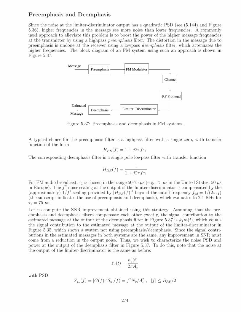
Preemphasis and Deemphasis

Since the noise at the limiter-discriminator output has a quadratic PSD (see (5.144) and Figure5.36), higher frequencies in the message see more noise than lower frequencies. A commonlyused approach to alleviate this problem is to boost the power of the higher message frequenciesat the transmitter by using a highpass preemphasis filter. The distortion in the message due topreemphasis is undone at the receiver using a lowpass deemphasis filter, which attenuates thehigher frequencies. The block diagram of an FM system using such an approach is shown inFigure 5.37.

Message

Channel

RF Frontend

Limiter−Discriminator

Preemphasis

Deemphasis

FM ModulatorMessage

Estimated

Figure 5.37: Preemphasis and deemphasis in FM systems.

A typical choice for the preemphasis filter is a highpass filter with a single zero, with transferfunction of the form

HPE(f) = 1 + j2πfτ1

The corresponding deemphasis filter is a single pole lowpass filter with transfer function

HDE(f) =1

1 + j2πfτ1

For FM audio broadcast, τ1 is chosen in the range 50-75 µs (e.g., 75 µs in the United States, 50 µsin Europe). The f 2 noise scaling at the output of the limiter-discriminator is compensated by the(approximately) 1/f 2 scaling provided by |HDE(f)|2 beyond the cutoff frequency fpd = 1/(2πτ1)(the subscript indicates the use of preemphasis and deemphasis), which evaluates to 2.1 KHz forτ1 = 75 µs.

Let us compute the SNR improvement obtained using this strategy. Assuming that the pre-emphasis and deemphasis filters compensate each other exactly, the signal contribution to theestimated message at the output of the deemphasis filter in Figure 5.37 is kfm(t), which equalsthe signal contribution to the estimated message at the output of the limiter-discriminator inFigure 5.35, which shows a system not using preemphasis/deemphasis. Since the signal contri-butions in the estimated messages in both systems are the same, any improvement in SNR mustcome from a reduction in the output noise. Thus, we wish to characterize the noise PSD andpower at the output of the deemphasis filter in Figure 5.37. To do this, note that the noise atthe output of the limiter-discriminator is the same as before:

zn(t) =n′s(t)

2πAc

with PSDSzn(f) = |G(f)|2Sns(f) = f 2N0/A

2c , |f | ≤ BRF/2

274

The noise vn obtained by passing zn through the deemphasis filter has PSD

Svn(f) = |HDE(f)|2Szn(f) =N0

A2c

f 2

1 + (f/fpd)2=N0f

2pd

A2c

(

1− 1

1 + (f/fpd)2

)

Integrating over the message bandwidth, we find that the noise power in the estimated messagein Figure 5.37 is given by

Pn =

∫ Bm

−Bm

Svn(f)df =2N0f

3pd

A2c

(

Bm

fpd− tan−1 Bm

fpd

)

(5.150)

where we have used the substitution tan x = f/fpd to evaluate the integral. As we have alreadymentioned, the signal power is unchanged from the earlier analysis, so that the improvement inSNR is given by the reduction in noise power compared with (5.145), which gives

SNRgain =

2B3mN0

3A2c

2N0f3pd

A2c

(

Bm

fpd− tan−1 Bm

fpd

) =1

3

(

Bm

fpd

)3

(

Bm

fpd− tan−1 Bm

fpd

) (5.151)

For fpd = 2.1 KHz, corresponding to the United States guidelines for FM audio broadcast, andan audio bandwidth Bm = 15 KHz, the SNR gain in (5.151) evaluates to more than 13 dB.

For completeness, we give the formula for the SNR obtained using preemphasis and deemphasisas

SNRFM,pd =

(

Bm

fpd

)3

(

Bm

fpd− tan−1 Bm

fpd

)

β2

PARSNRb (5.152)

which is obtained by taking the product of the SNR gain (5.151) and the SNR without preem-phasis/deemphasis given by (5.147).

275

Chapter 6

Optimal Demodulation

As we saw in Chapter 4, we can send bits over a channel by choosing one of a set of waveforms tosend. For example, when sending a single 16QAM symbol, we are choosing one of 16 passbandwaveforms:

sbc,bs = bcp(t) cos 2πfct− bsp(t) sin 2πfct

where bc, bs each take values in ±1,±3. We are thus able to transmit log2 16 = 4 bits ofinformation. In this chapter, we establish a framework for recovering these 4 bits when thereceived waveform is a noisy version of the transmitted waveform. More generally, we considerthe fundamental problem of M-ary signaling in additive white Gaussian noise (AWGN): one ofM signals, s1(t), ..., sM(t) is sent, and the received signal equals the transmitted signal plus whiteGaussian noise (WGN).

At the receiver, we are faced with a hypothesis testing problem: we have M possible hypothesesabout which signal was sent, and we have to make our “best” guess as to which one holds, basedon our observation of the received signal. We are interested in finding a guessing strategy, moreformally termed a decision rule, which is the “best” according to some criterion. For communi-cations applications, we are typically interested in finding a decision rule which minimizes theprobability of error (i.e., the probability of making a wrong guess). We can now summarize thegoals of this chapter as follows.

Goals: We wish to design optimal receivers when the received signal is modeled as follows:

Hi : y(t) = si(t) + n(t) , i = 1, , , .M

where Hi is the ith hypothesis, corresponding to signal si(t) being transmitted, and where n(t)is white Gaussian noise. We then wish to analyze the performance of such receivers, to see howperformance measures such as the probability of error depend on system parameters. It turnsout that, for the preceding AWGN model, the performance depends only on the received signal-to-noise ratio (SNR) and on the “shape” of the signal constellation s1(t), ..., sM(t). Underlyingboth the derivation of the optimal receiver and its analysis is a geometric view of signals andnoise as vectors, which we term signal space concepts. Once we have this background, we are ina position to discuss elementary power-bandwidth tradeoffs. For example, 16QAM has higherbandwidth efficiency than QPSK, so it makes sense that it has lower power efficiency; that is, itrequires higher SNR, and hence higher transmit power, for the same probability of error. We willbe able to quantify this intuition, previewed in Chapter 4, based on the material in this chapter.We will also be able to perform link budget calculations: for example, how much transmit poweris needed to attain a given bit rate using a given constellation as a function of range, and transmitand receive antenna gains?

Chapter Plan: The prerequisites for this chapter are Chapter 4 (digital modulation) and thematerial on Gaussian random variables (Section 5.6) and noise modeling (Section 5.8) in Chap-ter 5. We build up the remaining background required to attain our goals in this chapter in a

277

step-by-step fashion, as follows.Hypothesis testing: In Section 6.1, we establish the basic framework for hypothesis testing, de-rive the form of optimal decision rules, and illustrate the application of this framework forfinite-dimensional observations.Signal space concepts: In Section 6.2, we show that continuous time M-ary signaling in AWGNcan be reduced to an equivalent finite-dimensional system, in which transmitted signal vectorsare corrupted by vector WGN. This is done by projecting the continuous time signal into thefinite-dimensional signal space spanned by the set of possible transmitted signals, s1, ..., sM . Weapply the hypothesis testing framework to derive the optimal receiver for the finite-dimensionalsystem, and from this we infer the optimal receiver in continuous time.Performance analysis: In Section 6.3, we analyze the performance of optimal reception. We showthat performance depends only on SNR and the relative geometry of the signal constellation. Weprovide exact error probability expressions for binary signaling. While the probability of error forlarger signal constellations must typically be computed by simulation or numerical integration,we obtain bounds and approximations, building on the analysis for binary signaling, that providequick insight into power-bandwidth tradeoffs.Link budget analysis: In Section 6.5, we illustrate how performance analysis is applied to obtain-ing the “link budget” for a typical radio link, which is the tool used to obtain coarse guidelinesfor the design of hardware, including transmit power, transmit and receive antennas, and receivernoise figure.

Notational shortcut: In this chapter, we make extensive use of the notational simplificationdiscussed at the end of Section 5.3. Given a random variable X , a common notation for probabil-ity density function or probability mass function is pX(x), with X denoting the random variable,and x being a dummy variable which we might integrate out when computing probabilities.However, when there is no scope for confusion, we use the less cumbersome (albeit incomplete)notation p(x), using the dummy variable x not only as the argument of the density, but alsoto indicate that the density corresponds to the random variable X . (Similarly, we would usep(y) to denote the density for a random variable Y .) The same convention is used for joint andconditional densities as well. For random variables X and Y , we use the notation p(x, y) in-stead of pX,Y (x, y), and p(y|x) instead of pY |X(y|x), to denote the joint and conditional densities,respectively.

6.1 Hypothesis Testing

In Example 5.6.3, we considered a simple model for binary signaling, in which the receiver seesa single sample Y . If 0 is sent, the conditional distribution of Y is N(0, v2), while if 1 is sent,the conditional distribution is N(m, v2). We analyzed a simple decision rule in which we guessthat 0 is sent if Y ≤ m/2, and guess that 1 is sent otherwise. Thus, we wish to decide betweentwo hypotheses (0 being sent or 1 being sent) based on an observation (the received sample Y ).The statistics of the observation depend on the hypothesis (this information is captured by theconditional distributions of Y given each hypotheses). We must now make a good guess as towhich hypothesis is true, based on the value of the observation. The guessing strategy is calledthe decision rule, which maps each possible value of Y to either 0 or 1.

The decision rule we have considered in Example 5.6.3 makes sense, splitting the differencebetween the conditional means of Y under the two hypotheses. But is it always the best thingto do? For example, if we know for sure that 0 is sent, then we should clearly always guess that0 is sent, regardless of the value of Y that we see. As another example, if the noise variance isdifferent under the two hypotheses, then it is no longer clear that splitting the difference betweenthe means is the right thing to do. We therefore need a systematic framework for hypothesistesting, which allows us to derive good decision rules for a variety of statistical models.

278

In this section, we consider the general problem of M-ary hypothesis testing, in which we mustdecide which of M possible hypotheses, H0, ..., HM−1, “best explains” an observation Y . Forour purpose, the observation Y can be a scalar or vector, and takes values in an observationspace Γ. The link between the hypotheses and observation is statistical: for each hypothesisHi, we know the conditional distribution of Y given Hi. We denote the conditional densityof Y given Hi as p(y|i), i = 0, 1, ...,M − 1. We may also know the prior probabilities of thehypotheses (i.e., the probabillity of each hypothesis prior to seeing the observation), denoted by

πi = P [Hi], i = 0, 1, ...,M − 1, which satisfy∑M−1

i=0 π=1. The final ingredient of the hypothesistesting framework is the decision rule: for each possible value Y = y of the observation, we mustdecide which of the M hypotheses we will bet on. Denoting this guess as δ(y), the decision ruleδ(·) is a mapping from the observation space Γ to 0, 1, ...,M − 1, where δ(y) = i means thatwe guess that Hi is true when we see Y = y. The decision rule partitions the observation spaceinto decision regions, with Γi denoting the set of values of Y for which we guess Hi. That is,Γi = y ∈Γ : δ(y) = i, i = 0, 1, ...,M − 1. We summarize these ingredients of the hypothesistesting framework as follows.

Ingredients of hypothesis testing framework

• Hypotheses H0, H1, ..., HM−1

• Observation Y ∈Γ• Conditional densities p(y|i), for i = 0, 1, ...,M − 1• Prior probabilities πi = P [Hi], i = 0, 1, ...,M − 1, with

∑M−1i=0 πi = 1

• Decision rule δ : Γ → 0, 1, ...,M − 1• Decision regions Γi = y ∈Γ : δ(y) = i, i = 0, 1, ...,M − 1

To make the concepts concrete, let us quickly recall Example 5.6.3, where we have M = 2hypotheses, with H0 : Y ∼ N(0, v2) and H1 : Y ∼ N(m, v2). The “sensible” decision rule in thisexample can be written as

δ(y) =

0, y ≤ m/21, y > m/2

so that Γ0 = (−∞, m/2] and Γ1 = (m/2,∞). Note that this decision rule need not be optimalif we know the prior probabilities. For example, if we know that π0 = 1, we should say that H0

is true, regardless of the value of Y : this would reduce the probability of error from Q(

m2v

)

(forthe “sensible” rule) to zero!

6.1.1 Error probabilities

The performance measures of interest to us when choosing a decision rule are the conditionalerror probabilities and the average error probability. We have already seen these in Example5.6.3 for binary on-off keying, but we now formally define them for a general M-ary hypothesistesting problem. For a fixed decision rule δ with corresponding decision regions Γi, we definethe conditional probabilities of error as follows.

Conditional Error Probabilities: The conditional error probability, conditioned on Hi, where0 ≤ i ≤M − 1, is defined as

Pe|i = P [say Hj for some j 6= i|Hi is true] =∑

j 6=i

P [Y ∈Γj |Hi] = 1− P [Y ∈Γi|Hi] (6.1)

Conditional Probabilities of Correct Decision: These are defined as

Pc|i = 1− Pe|i = P [Y ∈Γi|Hi] (6.2)

279

Average Error Probability: This is given by averaging the conditional error probabilitiesusing the priors:

Pe =M∑

i=1

πiPe|i (6.3)

Average Probability of Correct Decision: This is given by

Pc =M∑

i=1

πiPc|i = 1− Pe (6.4)

6.1.2 ML and MAP decision rules

For a general M-ary hypothesis testing problem, an intuitively pleasing decision rule is themaximum likelihood rule, which, for a given observation Y = y, picks the hypothesis Hi for whichthe observed value Y = y is most likely; that is, we pick i so as to maximize the conditionaldensity p(y|i).Notation: We denote by “arg max” the argument of the maximum. That is, if the maximumof a function f(x) occurs at x0, then x0 is the argument of the maximum:

maxxf(x) = f(x0), arg maxxf(x) = x0

Note also that, while the maximum value of a function is changed if we apply another functionto it, if the second function is strictly increasing, then the argument of the maximum remains thesame. For example, when dealing with densities taking exponential forms (such as the Gaussian),it is useful to apply the logarithm (which is a strictly increasing function), as we note for the MLrule below.

Maximum Likelihood (ML) Decision Rule: The ML decision rule is defined as

δML(y) = arg max0≤i≤M−1 p(y|i) = arg max0≤i≤M−1 log p(y|i) (6.5)

Another decision rule that “makes sense” is the Maximum A Posteriori Probability (MAP) rule,where we pick the hypothesis which is most likely, conditioned on the value of the observation.The conditional probabilities P [Hi|Y = y] are called the a posteriori, or posterior, probabilities,since they are probabilities that we can compute after we see the observation Y = y. Let uswork through what this rule is actually doing. Using Bayes’ rule, the posterior probabilities aregiven by

P [Hi|Y = y] =p(y|i)P [Hi]

p(y)=πip(y|i)p(y)

, i = 0, 2., , , .,M − 1

Since we want to maximize this over i, the denominator p(y), the unconditional density of Y ,can be ignored in the maximization. We can also take the log as we did for the ML rule. TheMAP rule can therefore be summarized as follows.

Maximum A Posteriori Probability (MAP) Rule: The MAP decision rule isdefined as

δMAP (y) = arg max0≤i≤M−1 P [Hi|Y = y]= arg max1≤i≤M πip(y|i) = arg max0≤i≤M−1 log πi + log p(y|i) (6.6)

Properties of the MAP rule:• The MAP rule reduces to the ML rule for equal priors.

280

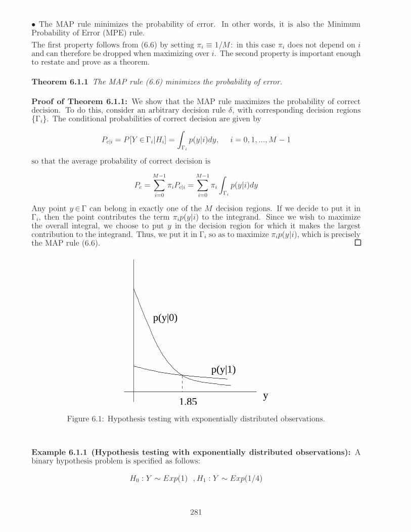
• The MAP rule minimizes the probability of error. In other words, it is also the MinimumProbability of Error (MPE) rule.

The first property follows from (6.6) by setting πi ≡ 1/M : in this case πi does not depend on iand can therefore be dropped when maximizing over i. The second property is important enoughto restate and prove as a theorem.

Theorem 6.1.1 The MAP rule (6.6) minimizes the probability of error.

Proof of Theorem 6.1.1: We show that the MAP rule maximizes the probability of correctdecision. To do this, consider an arbitrary decision rule δ, with corresponding decision regionsΓi. The conditional probabilities of correct decision are given by

Pc|i = P [Y ∈Γi|Hi] =

∫

Γi

p(y|i)dy, i = 0, 1, ...,M − 1

so that the average probability of correct decision is

Pc =

M−1∑

i=0

πiPc|i =

M−1∑

i=0

πi

∫

Γi

p(y|i)dy

Any point y ∈Γ can belong in exactly one of the M decision regions. If we decide to put it inΓi, then the point contributes the term πip(y|i) to the integrand. Since we wish to maximizethe overall integral, we choose to put y in the decision region for which it makes the largestcontribution to the integrand. Thus, we put it in Γi so as to maximize πip(y|i), which is preciselythe MAP rule (6.6).

1.85

p(y|0)

p(y|1)

y

Figure 6.1: Hypothesis testing with exponentially distributed observations.

Example 6.1.1 (Hypothesis testing with exponentially distributed observations): Abinary hypothesis problem is specified as follows:

H0 : Y ∼ Exp(1) , H1 : Y ∼ Exp(1/4)

281

where Exp(µ) denotes an exponential distribution with density µe−µy, CDF 1 − e−µy and com-plementary CDF e−µy, where y ≥ 0 (all the probability mass falls on the nonnegative numbers).Note that the mean of an Exp(µ) random variable is 1/µ. Thus, in our case, the mean under H0

is 1, while the mean under H1 is 4.(a) Find the ML rule and the corresponding conditional error probabilities.(b) Find the MPE rule when the prior probability of H1 is 1/5. Also find the conditional andaverage error probabilities.Solution:(a) As shown in Figure 6.1, we have

p(y|0) = e−yIy≥0 , p(y|1) = (1/4)e−y/4Iy≥0

The ML rule is given by

p(y|1)H1

><H0

p(y|0)

which reduces to

(1/4)e−y/4

H1

><H0

e−y (y ≥ 0)

Taking logarithms on both sides and simplifying, we obtain that the ML rule is given by

y

H1

><H0

(4/3) log 4 = 1.8484

The conditional error probabilities are

Pe|0 = P [say H1|H0] = P [Y > (4/3) log 4|H0]= e−(4/3) log 4 = (1/4)4/3 = 0.1575

Pe|1 = P [say H0|H1] = P [Y ≤ (4/3) log 4|H1]= 1− e−(1/3) log 4 = 1− (1/4)1/3 = 0.37

These conditional error probabilities are rather high, telling us that exponentially distributedobservations with different means do not give us high-quality information about the hypotheses.(b) The MPE rule is given by

π1p(y|1)H1

><H0

π0p(y|0)

which reduces to

(1/5) (1/4)e−y/4

H1

><H0

(4/5) e−y

282

This gives

y

H1

><H0

4

3log 16 = 3.6968

Proceeding as in (a), we obtain

Pe|0 = e−(4/3) log 16 = (1/16)4/3 = 0.0248

Pe|1 = 1− e−(1/3) log 16 = 1− (1/16)1/3 = 0.6031

with average error probability

Pe = π0Pe|0 + π1Pe|1 = (4/5) ∗ 0.0248 + (1/5) ∗ 0.6031 = 0.1405

Since the prior probability of H1 is small, the MPE rule is biased towards guessing that H0 istrue. In this case, the decision rule is so skewed that the conditional probability of error underH1 is actually worse than a random guess. Taking this one step further, if the prior probabilityof H1 actually becomes zero, then the MPE rule would always guess that H0 is true. In this case,the conditional probability of error under H1 would be one! This shows that we must be carefulabout modeling when applying the MAP rule: if we are wrong about our prior probabilities, andH1 does occur with nonzero probability, then our performance would be quite poor.

Both the ML and MAP rules involve comparison of densities, and it is convenient to expressthem in terms of a ratio of densities, or likelihood ratio, as discussed next.

Binary hypothesis testing and the likelihood ratio: For binary hypothesis testing, the MLrule (6.5) reduces to

p(y|1)H1

><H0

p(y|0) , orp(y|1)p(y|0)

H1

><H0

1 (6.7)

The ratio of conditional densities appearing above is defined to be the likelihood ratio (LR) L(y)a function of fundamental importance in hypothesis testing. Formally, we define the likelihoodratio as

L(y) =p(y|1)p(y|0) , y ∈Γ (6.8)

Likelihood ratio test: A likelihood ratio test (LRT) is a decision rule in which we compare thelikelihood ratio to a threshold.

L(y)

H1

><H0

γ

where the choice of γ depends on our performance criterion. An equivalent form is the loglikelihood ratio test (LLRT), where the log of the likelihood ratio is compared with a threshold.

We have already shown in (6.7) that the ML rule is an LRT with threshold γ = 1. From (6.6),we see that the MAP, or MPE, rule is also an LRT:

π1p(y|1)H1

><H0

π0p(y|0) , orp(y|1)p(y|0)

H1

><H0

π0π1

283

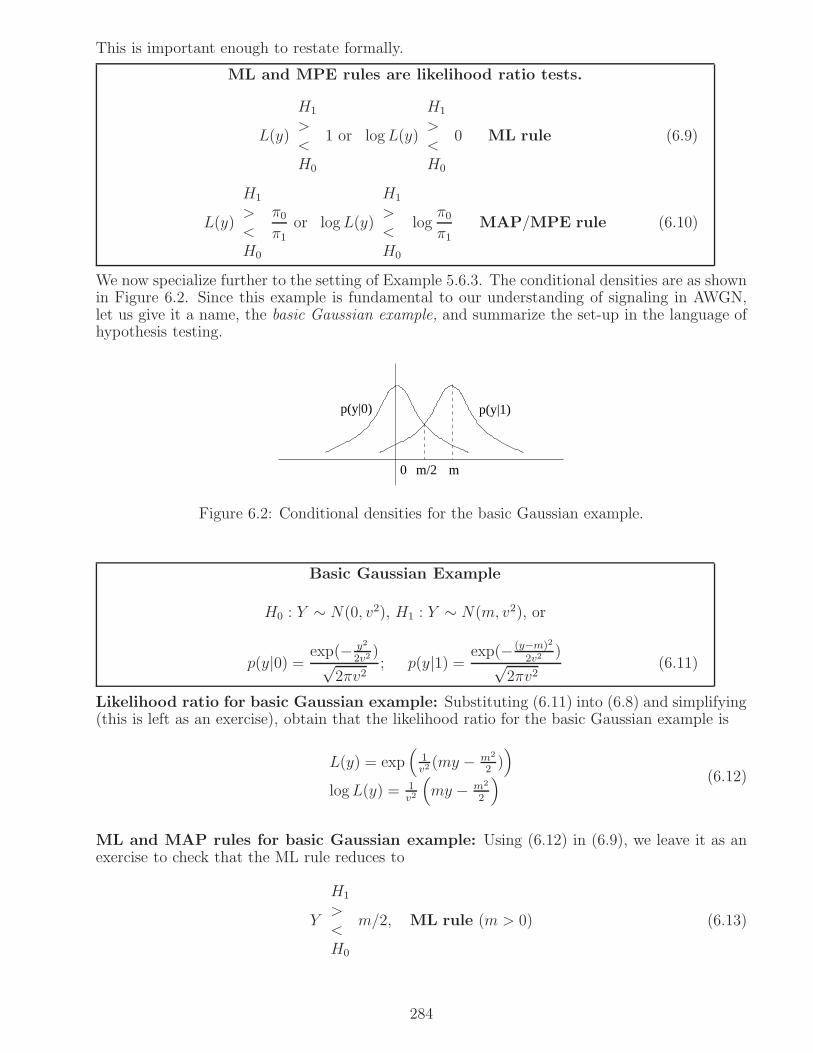
This is important enough to restate formally.

ML and MPE rules are likelihood ratio tests.

L(y)

H1

><H0

1 or logL(y)

H1

><H0

0 ML rule (6.9)

L(y)

H1

><H0

π0π1

or logL(y)

H1

><H0

logπ0π1

MAP/MPE rule (6.10)

We now specialize further to the setting of Example 5.6.3. The conditional densities are as shownin Figure 6.2. Since this example is fundamental to our understanding of signaling in AWGN,let us give it a name, the basic Gaussian example, and summarize the set-up in the language ofhypothesis testing.

m/20 m

p(y|1)p(y|0)

Figure 6.2: Conditional densities for the basic Gaussian example.

Basic Gaussian Example

H0 : Y ∼ N(0, v2), H1 : Y ∼ N(m, v2), or

p(y|0) = exp(− y2

2v2)√

2πv2; p(y|1) = exp(− (y−m)2

2v2)√

2πv2(6.11)

Likelihood ratio for basic Gaussian example: Substituting (6.11) into (6.8) and simplifying(this is left as an exercise), obtain that the likelihood ratio for the basic Gaussian example is

L(y) = exp(

1v2(my − m2

2))

logL(y) = 1v2

(

my − m2

2

) (6.12)

ML and MAP rules for basic Gaussian example: Using (6.12) in (6.9), we leave it as anexercise to check that the ML rule reduces to

Y

H1

><H0

m/2, ML rule (m > 0) (6.13)

284

(check that the inequalities get reversed for m < 0). This is exactly the “sensible” rule that weanalyzed in Example 5.6.3. Using (6.12) in (6.10), we obtain the MAP rule:

Y

H1

><H0

m/2 +v2

mlog

π0π1, MAP rule (m > 0) (6.14)

Example 6.1.2 (ML versus MAP for the basic Gaussian example): For the basic Gaus-sian example, we now know that the decision rule in Example 5.6.3 is the ML rule, and weshowed in that example that the performance of this rule is given by

Pe|0 = Pe|1 = Pe = Q(m

2v

)

= Q(

√

SNR/2)

We also saw that at 13 dB SNR, the error probability for the ML rule is

Pe,ML = 7.8× 10−4

regardless of the prior probabilities. For equal priors, the ML rule is also MPE, and we cannothope to do better than this. Let us now see what happens when the prior probability of H0 isπ0 =

13. The ML rule is no longer MPE, and we should be able to do better by using the MAP

rule. We leave it as an exercise to show that the conditional error probabilities for the MAP ruleare given by

Pe|0 = Q

(

m

2v+v

mlog

π0π1

)

, Pe|1 = Q

(

m

2v− v

mlog

π0π1

)

(6.15)

Plugging in the numbers for SNR of 13 dB and π0 =13, we obtain

Pe|0 = 1.1× 10−3 , Pe|1 = 5.34× 10−4

which averages toPe,MAP = 7.3× 10−4

a slight improvement on the error probability of the ML rule.

Figure 6.3 shows the results of further numerical experiments (see caption for discussion).

6.1.3 Soft Decisions

We have so far considered hard decision rules in which we must choose exactly one of the Mhypotheses. In doing so, we are throwing away a lot of information in the observation. Forexample, suppose that we are testing H0 : Y ∼ N(0, 4) versus H1 : Y ∼ N(10, 4) with equal

priors, so that the MPE rule is Y

H1

><H0

5. We would guess H1 if Y = 5.1 as well as if Y = 10.3,

but we would be a lot more confident about our guess in the latter instance. Rather thanthrowing away this information, we can employ soft decisions that convey reliability informationwhich could be used at a higher layer, for example, by a decoder which is processing a codewordconsisting of many bits.

Actually, we already know how to compute soft decisions: the posterior probabilities P [Hi|Y = y],i = 0, 1, ...,M − 1, that appear in the MAP rule are actually the most information that we can

285

3 4 5 6 7 8 9 1010

−3

10−2

10−1

100

SNR (dB)

Err

or P

roba

bilit

ies

P(error) (ML)P(error) (MAP)P(error|0) (MAP)P(error|1) (MAP)

(a) Dependence on SNR (π0 = 0.3)

0 0.1 0.2 0.3 0.4 0.5 0.6 0.7 0.8 0.9 110

−4

10−3

10−2

10−1

100

Prior Probability of H0

Err

or P

roba

bilit

ies

P(error) (ML)P(error) (MAP)P(error|0) (MAP)P(error|1) (MAP)

(b) Dependence on priors (SNR = 10 dB)

Figure 6.3: Conditional and average error probabilities for the MAP receiver compared to theerror probability for the ML receiver. We consider the basic Gaussian example, fixing the priorsand varying SNR in (a), and fixing SNR and varying the priors in (b). For the MAP rule,the conditional error probability given a hypothesis increases as the prior probability of thehypothesis decreases. The average error probability for the MAP rule is always smaller than theML rule (which is the MAP rule for equal priors) when π0 6= 1

2. The MAP error probability

tends towards zero as π0 → 0 or π0 → 1.

hope to get about the hypotheses from the observation. For notational compactness, let usdenote these by πi(y). The posterior probabilities can be computed using Bayes’ rule as follows:

πi(y) = P [Hi|Y = y] =πip(y|i)p(y)

=πip(y|i)

∑M−1j=0 πjp(y|j)

(6.16)

In practice, we may settle for quantized soft decisions which convey less information than theposterior probabilities due to tradeoffs in precision or complexity versus performance.

Example 6.1.3 (Soft decisions for 4PAM in AWGN): Consider a 4-ary hypothesis testingproblem modeled as follows:

H0 : Y ∼ N(−3A, σ2) , H1 : Y ∼ N(−A, σ2) , H2 : Y ∼ N(A, σ2) , H3 : Y ∼ N(3A, σ2)

This is a model that arises for 4PAM signaling in AWGN, as we see later. For σ2 = 1, A = 1and Y = −1.5, find the posterior probabilities if π0 = 0.4 and π1 = π2 = π3 = 0.2.Solution: The posterior probability for the ith hypothesis is of the form

πi(y) = c πie− (y−mi)

2

2σ2

where mi ∈±A,±3A is the conditional mean under Hi, and where c is a constant that doesnot depend on i. Since the posterior probabilities must sum to one, we have

3∑

j=0

πj(y) = c3∑

j=0

πje− (y−mj)

2

2σ2 = 1

Solving for c, we obtain

πi(y) =πie

− (y−mi)2

2σ2

∑3j=0 πje

− (y−mj)2

2σ2

286

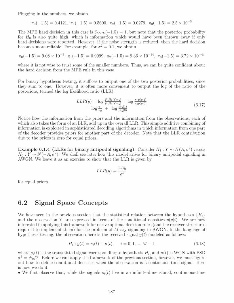
Plugging in the numbers, we obtain

π0(−1.5) = 0.4121, π1(−1.5) = 0.5600, π2(−1.5) = 0.0279, π3(−1.5) = 2.5× 10−5

The MPE hard decision in this case is δMPE(−1.5) = 1, but note that the posterior probabilityfor H0 is also quite high, which is information which would have been thrown away if onlyhard decisions were reported. However, if the noise strength is reduced, then the hard decisionbecomes more reliable. For example, for σ2 = 0.1, we obtain

π0(−1.5) = 9.08× 10−5, π1(−1.5) = 0.9999, π2(−1.5) = 9.36× 10−14, π3(−1.5) = 3.72× 10−44

where it is not wise to trust some of the smaller numbers. Thus, we can be quite confident aboutthe hard decision from the MPE rule in this case.

For binary hypothesis testing, it suffices to output one of the two posterior probabilities, sincethey sum to one. However, it is often more convenient to output the log of the ratio of theposteriors, termed the log likelihood ratio (LLR):

LLR(y) = log P [H1|Y=y]P [H0|Y=y]

= log π1p(y|1)π0p(y|0)

= log π1

π0+ log p(y|1)

p(y|0)(6.17)

Notice how the information from the priors and the information from the observations, each ofwhich also takes the form of an LLR, add up in the overall LLR. This simple additive combining ofinformation is exploited in sophisticated decoding algorithms in which information from one partof the decoder provides priors for another part of the decoder. Note that the LLR contributiondue to the priors is zero for equal priors.

Example 6.1.4 (LLRs for binary antipodal signaling): ConsiderH1 : Y ∼ N(A, σ2) versusH0 : Y ∼ N(−A, σ2). We shall see later how this model arises for binary antipodal signaling inAWGN. We leave it as an exercise to show that the LLR is given by

LLR(y) =2Ay

σ2

for equal priors.

6.2 Signal Space Concepts

We have seen in the previous section that the statistical relation between the hypotheses Hiand the observation Y are expressed in terms of the conditional densities p(y|i). We are nowinterested in applying this framework for derive optimal decision rules (and the receiver structuresrequired to implement them) for the problem of M-ary signaling in AWGN. In the language ofhypothesis testing, the observation here is the received signal y(t) modeled as follows:

Hi : y(t) = si(t) + n(t), i = 0, 1, ...,M − 1 (6.18)

where si(t) is the transmitted signal corresponding to hypothesis Hi, and n(t) is WGN with PSDσ2 = N0/2. Before we can apply the framework of the previous section, however, we must figureout how to define conditional densities when the observation is a continuous-time signal. Hereis how we do it:• We first observe that, while the signals si(t) live in an infinite-dimensional, continuous-time

287

space, if we are only interested in the M signals that could be transmitted under each of the Mhypotheses, then we can limit attention to a finite-dimensional subspace of dimension at mostM . We call this the signal space. We can then express the signals as vectors corresponding toan expansion with respect to an orthonormal basis for the subspace.• The projection of WGN onto the signal space gives us a noise vector whose components arei.i.d. Gaussian. Furthermore, we observe that the component of the received signal orthogonal tothe signal space is irrelevant: that is, we can throw it away without compromising performance.• We can therefore restrict attention to projection of the received signal onto the signal spacewithout loss of performance. This projection can be expressed as a finite-dimensional vectorwhich is modeled as a discrete time analogue of (6.18). We can now apply the hypothesis testingframework of Section 6.1 to infer the optimal (ML and MPE) decision rules.• We then translate the optimal decision rules back to continuous time to infer the structure ofthe optimal receiver.

6.2.1 Representing signals as vectors

Let us begin with an example illustrating how continuous-time signals can be represented asfinite-dimensional vectors by projecting onto the signal space.

16QAMQPSK/4PSK/4QAM 8PSK

Figure 6.4: For linear modulation with no intersymbol interference, the complex symbols them-selves provide a two-dimensional signal space representation. Three different constellations areshown here.

Example 6.2.1 (Signal space for two-dimensional modulation): Consider a single complex-valued symbol b = bc + jbs (assume that there is no intersymbol interference) sent using two-dimensional passband linear modulation. The set of possible transmitted signals are given by

sbc,bs(t) = bcp(t) cos 2πfct− bsp(t) sin 2πfct

where (bc, bs) takesM possible values for anM-ary constellation (e.g.,M = 4 for QPSK,M = 16for 16QAM), and where p(t) is a baseband pulse of bandwidth smaller than the carrier frequencyfc. Setting φc(t) = p(t) cos 2πfct and φs(t) = −p(t) sin 2πfct, we see that we can write the set oftransmitted signals as a linear combination of these signals as follows:

sbc,bs(t) = bcφc(t) + bsφs(t)

so that the signal space has dimension at most 2. From Chapter 2, we know that φc and φs

are orthogonal (I-Q orthogonality), and hence linearly independent. Thus, the signal space hasdimension exactly 2. Noting that ||φc||2 = ||φs||2 = 1

2||p||2, the normalized versions of φc and φs

provide an orthonormal basis for the signal space:

ψc(t) =φc(t)

||φc||, ψs(t) =

φs(t)

||φs||

288

We can now write

sbc,bs(t) =1√2||p||bcψc(t) +

1√2||p||bsψs(t)

With respect to this basis, the signals can be represented as two dimensional vectors:

sbc,bs(t) ↔ sbc,bs =1√2||p||

(

bcbs

)

That is, up to scaling, the signal space representation for the transmitted signals are simply thetwo-dimensional symbols (bc, bs)

T . Indeed, while we have been careful about keeping track ofthe scaling factor in this example, we shall drop it henceforth, because, as we shall soon see,what matters in performance is the signal-to-noise ratio, rather than the absolute signal or noisestrength.

Orthogonal modulation provides another example where an orthonormal basis for the signalspace is immediately obvious. For example, if s1, ..., sM are orthogonal signals with equal energy

||s||2 ≡ Es, then ψi(t) =si(t)√Es

provide an orthonormal basis for the signal space, and the vector

representation of the ith signal is the scaled unit vector√Es(0, ..., 0, 1( in ith position), 0, ..., 0)T .

Yes another example where an orthonormal basis can be determined by inspection is shown inFigures 6.5 and 6.6, and discussed in Example 6.2.2.

−1

s (t) s (t)1

3s (t)s (t)2

0

11

10

2

0 2

1

t t

t t

−1

3

3 31

31

0

Figure 6.5: Four signals spanning a three-dimensional signal space

30

1 1

ψ (t) ψ (t) ψ (t)0 1 2

1

0 tt

11 2t

2

Figure 6.6: An orthonormal basis for the signal set in Figure 6.5, obtained by inspection.

Example 6.2.2 (Developing a signal space representation for a 4-ary signal set): Con-sider the example depicted in Figure 6.5, where there are 4 possible transmitted signals, s0, ..., s3.

289

It is clear from inspection that these span a three-dimensional signal space, with a convenientchoice of basis signals

ψ0(t) = I[0,1](t), ψ1(t) = I[1,2](t), ψ2(t) = I[2,3](t)

as shown in Figure 6.6. Let si = (si[1], si[2], si[3])T denote the vector representation of the signal

si with respect to the basis, for i = 0, 1, 2, 3. That is, the coefficients of the vector si are suchthat

si(t) =

2∑

k=0

si[k]ψk(t)

we obtain, again by inspection, that

s0 =

111

, s1 =

−111

, s2 =

021

, s3 =

1−11

Now that we have seen some examples, it is time to be more precise about what we meanby the “signal space.” The signal space S is the finite-dimensional subspace (of dimensionn ≤ M) spanned by s0(t), ..., sM−1(t). That is, S consists of all signals of the form a0s0(t) +... + aM−1sM−1(t), where a0, ..., aM−1 are arbitrary scalars. Let ψ0(t), ..., ψn−1(t) denote an or-thonormal basis for S. We have seen in the preceding examples that such a basis can often bedetermined by inspection. In general, however, given an arbitrary set of signals, we can alwaysconstruct an orthonormal basis using the Gram-Schmidt procedure described below. We do notneed to use this procedure often–in most settings of interest, the way to go from continuous todiscrete time is clear–but state it below for completeness.

1

s (t)

1s (t)

(t)φ

||φ ||1

1ψ (t)1

(t)ψ0

||φ ||

(t)φ0

0

(t)φ0=

=

=

(t)φ

0

Figure 6.7: Illustrating Step 0 and Step 1 of the Gram-Schmidt procedure.

Gram-Schmidt orthogonalization: The idea is to build up an orthonormal basis step bystep, with the basis after the mth step spanning the first m signals. The first basis function isa scaled version of the first signal (assuming this is nonzero–otherwise we proceed to the secondsignal without adding a basis function). We then consider the component of the second signalorthogonal to the first basis function. This projection is nonzero if the second signal is linearlyindependent of the first; in this case, we introduce a basis function that is a scaled version ofthe projection. See Figure 6.7. This procedure goes on until we have covered all M signals. Thenumber of basis functions n equals the dimension of the signal space, and satisfies n ≤ M . Wecan summarize the procedure as follows.

290

Letting Sk−1 denote the subspace spanned by s0, ..., sk−1, the Gram-Schmidt algorithm proceedsiteratively: given an orthonormal basis for Sk−1, it finds an orthonormal basis for Sk. Theprocedure stops when k = M . The method is identical to that used for finite-dimensionalvectors, except that the definition of the inner product involves an integral, rather than a sum,for the continuous-time signals considered here.

Step 0 (Initialization): Let φ0 = s0. If φ0 6= 0, then set ψ0 = φ0

||φ0|| . Note that ψ0 provides a

basis function for S0.

Step k: Suppose that we have constructed an orthonormal basis Bk−1 = ψ0, ...ψm−1 for thesubspace Sk−1 spanned by the first k signals, s0, ..., sk−1 (note that m ≤ k). Define

φk(t) = sk(t)−m−1∑

i=0

〈sk, ψi〉ψi(t)

The signal φk(t) is the component of sk(t) orthogonal to the subspace Sk−1. If φk 6= 0, define

a new basis function ψm(t) =φk(t)||φk|| , and update the basis as Bk = ψ1, ..., ψm, ψm. If φk = 0,

then sk ∈Sk−1, and it is not necessary to update the basis; in this case, we set Bk = Bk−1 =ψ0, ..., ψm−1.The procedure terminates at step M , which yields a basis B = ψ0, ..., ψn−1 for the signal spaceS = SM−1. The basis is not unique, and may depend (and typically does depend) on the order inwhich we go through the signals in the set. We use the Gram-Schmidt procedure here mainly asa conceptual tool, in assuring us that there is indeed a finite-dimensional vector representationfor a finite set of continuous-time signals.

3

−2B

B C

−C

ψ0

(t)1

ψ (t)2

ψ (t)

A

t tt0 3 1 30 1 2

Figure 6.8: An orthonormal basis for the signal set in Figure 6.5, obtained by applying theGram-Schmidt procedure. The unknowns A, B, and C are to be determined in Exercise 6.2.1.

Exercise 6.2.1 (Application of the Gram-Schmidt procedure): Apply the Gram-Schmidtprocedure to the signal set in Figure 6.5. When the signals are considered in increasing order ofindex in the Gram-Schmidt procedure, verify that the basis signals are as in Figure 6.8, and fillin the missing numbers. While the basis thus obtained is not as “nice” as the one obtained byinspection in Figure 6.6, the Gram-Schmidt procedure has the advantage of general applicability.

Inner products are preserved: We shall soon see that the performance of M-ary signalingin AWGN depends only on the inner products between the signals, if the noise PSD is fixed.Thus, an important observation when mapping the continuous time hypothesis testing problemto discrete time is to check that these inner products are preserved when projecting onto thesignal space. Consider the continuous time inner products

〈si, sj〉 =∫

si(t)sj(t)dt , i, j = 0, 1, ...,M − 1 (6.19)

291

Now, expressing the signals in terms of their basis expansions, we have

si(t) =

n−1∑

k=0

si[k]ψk(t) , i = 0, 1, ...,M − 1

Plugging into (6.19), we obtain

〈si, sj〉 =∫ n−1∑

k=0

si[k]ψk(t)n−1∑

l=0

sj [l]ψl(t)dt

Interchanging integral and summations, we obtain

〈si, sj〉 =n−1∑

k=0

n−1∑

l=0

si[k]sj[l]

∫

ψk(t)ψl(t)dt

By the orthonormality of the basis functions ψk, we have

〈ψk, ψl〉 =∫

ψk(t)ψl(t)dt = δkl =

1, k = l0, k 6= l

This collapses the two summations into one, so that we obtain

〈si, sj〉 =∫

si(t)sj(t)dt =

n−1∑

k=0

si[k]sj[k] = 〈si, sj〉 (6.20)

where the extreme right-hand side is the inner product of the signal vectors si = (si[0], ..., si[n−1])T and sj = (sj[0], ..., sj [n−1])T . This makes sense: the geometric relationship between signals(which is what the inner products capture) should not depend on the basis with respect to whichthey are expressed.

6.2.2 Modeling WGN in signal space

What happens to the noise when we project onto the signal space? Define the noise projectiononto the ith basis function as

Ni = 〈n, ψi〉 =∫

n(t)ψi(t)dt , i = 0, 1, ..., n− 1 (6.21)

Then we can write the noise n(t) as follows:

n(t) =

n−1∑

i=0

Niψi(t) + n⊥(t)

where n⊥(t) is the projection of the noise orthogonal to the signal space. Thus, we can decom-pose the noise into two parts: a noise vector N = (N0, ..., Nn−1)

T corresponding to the projectiononto the signal space, and a component n⊥(t) orthogonal to the signal space. In order to charac-terize the statistics of these quantities, we need to consider random variables obtained by linearprocessing of WGN. Specifically, consider random variables generated by passing WGN throughcorrelators:

Z1 =

∫ ∞

−∞n(t)u1(t)dt = 〈n, u1〉

Z2 =

∫ ∞

−∞n(t)u2(t)dt = 〈n, u2〉

where u1 and u2 are deterministic, finite energy signals. We can now state the following result.

292

Theorem 6.2.1 (WGN through correlators): The random variables Z1 = 〈n, u1〉 and Z2 =〈n, u2〉 are zero mean, jointly Gaussian, with

cov(Z1, Z2) = cov (〈n, u1〉, 〈n, u2〉) = σ2〈u1, u2〉

Specializing to u1 = u2 = u, we obtain that

var(〈n, u〉) = cov(〈n, u〉, 〈n, u〉) = σ2||u||2

Thus, we obtain that Z = (Z1, Z2)T ∼ N(0,C) with covariance matrix

C =

(

σ2||u1||2 σ2〈u1, u2〉σ2〈u1, u2〉 σ2||u2||2

)

Proof of Theorem 6.2.1: The random variables Z1 = 〈n, u1〉 and Z2 = 〈n, u2〉 are zero meanand jointly Gaussian, since n is zero mean and Gaussian. Their covariance is computed as

cov (〈n, u1〉, 〈n, u2〉) = E [〈n, u1〉〈n, u2〉] = E[∫

n(t)u1(t)dt∫

n(s)u2(s)ds]

=∫ ∫

u1(t)u2(s)E[n(t)n(s)]dt ds =∫ ∫

u1(t)u2(s)σ2δ(t− s)dt ds

= σ2∫

u1(t)u2(t)dt = σ2〈u1, u2〉

The preceding computation is entirely analogous to the ones we did in Example 5.8.2 and inSection 5.10, but it is important enough that we repeat some points that we had mentionedthen. First, we need to use two different variables of integration, t and s, in order to make surewe capture all the cross terms. Second, when we take the expectation inside the integrals, wemust group all random terms inside it. Third, the two integrals collapse into one because theautocorrelation function of WGN is impulsive. Finally, specializing the covariance to get thevariance leads to the remaining results stated in the theorem.

We can now provide the following geometric interpretation of WGN.

Remark 6.2.1 (Geometric interpretation of WGN): Theorem 6.2.1 implies that the pro-jection of WGN along any “direction” in the space of signals (i.e., the result of correlating WGNwith a unit energy signal) has variance σ2 = N0/2. Also, its projections in orthogonal directionsare jointly Gaussian and uncorrelated random variables, and are therefore independent.

Noise projection on the signal space is discrete time WGN: It follows from the precedingremark that the noise projections Ni = 〈n, ψi〉 along the orthonormal basis functions ψi forthe signal space are i.i.d. N(0, σ2) random variables. In other words, the noise vector N =(N0, ..., Nn−1)

T ∼ N (0, σ2I). In other word, the components of N constitute discrete time whiteGaussian noise (“white” in this case means uncorrelated and having equal variance across allcomponents).

6.2.3 Hypothesis testing in signal space

Now that we have the signal and noise models, we can put them together in our hypothesistesting framework. Let us condition on hypothesis Hi. The received signal is given by

y(t) = si(t) + n(t) (6.22)

Projecting this onto the signal space by correlating against the orthonormal basis functions, weget

Y [k] = 〈y, ψk〉 = 〈si + n, ψk〉 = si[k] +N [k] , k = 0, 1., , , .n− 1

293

Signal space (finite−dimensional)

s

s1

sM−1

n (t)

N

(infinite−dimensional waveform)

0

Figure 6.9: Illustration of signal space concepts. The noise projection n⊥(t) orthogonal to thesignal space is irrelevant. The relevant part of the received signal is the projection onto the signalspace, which equals the vector Y = si +N under hypothesis Hi.

Collecting these into an n-dimensional vector, we get the model

Hi : Y = si +N

Note that the vector Y = (y[1], ..., y[n])T completely describes the component of the receivedsignal y(t) in the signal space, given by

yS(t) =n−1∑

j=0

〈y, ψj〉ψj(t) =n−1∑

j=0

Y [j]ψj(t)

The component of the received signal orthogonal to the signal space is given by

y⊥(t) = y(t)− yS(t)

It is shown in Appendix 6.A that this component is irrelevant to our decision. There are tworeasons for this, as elaborated in the appendix: first, there is no signal contribution orthogonalto the signal space (by definition); second, for the WGN model, the noise component orthogonalto the signal space carries no information regarding the noise vector in the signal space. As illus-trated in Figure 6.9, this enables us to reduce our infinite-dimensional problem to the followingfinite-dimensional vector model, without loss of optimality.

Model for received vector in signal space

Hi : Y = si +N , i = 0, 1, ...,M − 1 (6.23)

where N ∼ N(0, σ2I).

Two-dimensional modulation (Example 6.2.1 revisited): For a single symbol sent usingtwo-dimensional modulation, we have the hypotheses

Hbc,bs : y(t) = sbc,bs(t) + n(t)

wheresbc,bs(t) = bcp(t) cos 2πfct− bsp(t) sin 2πfct

294

Ys

3s s2

Nc

Ns

s0

N

1

Figure 6.10: A signal space view of QPSK. In the scenario shown, s0 is the transmitted vector,and Y = s0 + N is the received vector after noise is added. The noise components Nc, Ns arei.i.d. N(0, σ2) random variables.

Restricting attention to the two-dimensional signal space identified in the example, we obtainthe model

Hbc,bs : Y =

(

YcYs

)

=

(

bcbs

)

+

(

Nc

Ns

)

where we have absorbed scale factors into the symbol (bc, bs), and where the I and Q noise compo-nents Nc, Ns are i.i.d. N(0, σ2). This is illustrated for QPSK in Figure 6.10. Thus, conditionedon Hbc,bs, Yc ∼ N(bc, σ

2) and Ys ∼ N(bs, σ2), and Yc, Ys are conditionally independent. The

conditional density of Y = (Yc, Ys)T conditioned on Hbc,bs is therefore given by

p(yc, ys|bc, bs) =1

2σ2e−(yc−bc)2/(2σ2) 1

2σ2e−(ys−bs)2/(2σ2)

We can now infer the ML and MPE rules using our hypothesis testing framework. However, sincethe same reasoning applies to signal spaces of arbitrary dimensions, we provide a more generaldiscussion in the next section, and then return to examples of two-dimensional modulation.

6.2.4 Optimal Reception in AWGN

We begin by characterizing the optimal receiver when the received signal is a finite-dimensionalvector. Using this, we infer the optimal receiver for continuous-time received signals.

Demodulation for M-ary signaling in discrete time AWGN corresponds to solving an M-aryhypothesis testing problem with observation model as follows:

Hi : Y = si +N i = 0, 1, ...,M − 1 (6.24)

where N ∼ N(0, σ2I) is discrete time WGN. The ML and MPE rules for this problem are givenas follows. As usual, we denote the prior probabilities required to specify the MPE rule byπi, i = 1, ..,M (

∑M−1i=0 πi = 1).

295

Optimal Demodulation for Signaling in Discrete Time AWGN

ML ruleδML(y) = arg min0≤i≤M−1 ||y− si||2

= arg max0≤i≤M−1 〈y, si〉 − ||si||22

(6.25)

MPE rule

δMPE(y) = arg min0≤i≤M−1 ||y− si||2 − 2σ2 log πi= arg max0≤i≤M−1 〈y, si〉 − ||si||2

2+ σ2 log πi

(6.26)

Interpretation of optimal decision rules: The ML rule can be interpreted in two ways.The first is as a minimum distance rule, choosing the transmitted signal which has minimumEuclidean distance to the noisy received signal. The second is as a “template matcher”: choosingthe transmitted signal with highest correlation with the noisy received signal, while adjustingfor the fact that the energies of different transmitted signals may be different. The MPE ruleadjusts the ML cost function to reflect prior information: the adjustment term depends on thenoise level and the prior probabilities. The MPE cost functions decompose neatly into a sum ofthe ML cost function (which depends on the observation) and a term reflecting prior knowledge(which depends on the prior probabilities and the noise level). The latter term scales with thenoise variance σ2. Thus, we rely more on the observation at high SNR (small σ), and more onprior knowledge at low SNR (large σ).

Derivation of optimal receiver structures (6.25) and (6.26): Under hypothesis Hi, Y isa Gaussian random vector with mean si and covariance matrix σ2I (the translation of the noisevector N by the deterministic signal vector si does not change the covariance matrix), so that

pY|i(y|Hi) =1

(2πσ2)n/2exp(−||y− si||2

2σ2) (6.27)

Plugging (6.27) into the ML rule (6.5, we obtain the rule (6.25) upon simplification. Similarly,we obtain (6.26) by substituting (6.27) in the MPE rule (6.6).

We now map the optimal decision rules in discrete time back to continuous time to obtain optimaldetectors for the original continuous-time model (6.18), as follows.

Optimal Demodulation for Signaling in Continuous Time AWGN

ML rule

δML(y) = arg max0≤i≤M−1 〈y, si〉 −||si||22

(6.28)

MPE rule

δMPE(y) = arg max0≤i≤M−1 〈y, si〉 −||si||22

+ σ2 log πi (6.29)

Derivation of optimal receiver structures (6.28) and (6.29): Due to the irrelevance of y⊥,the continuous time model (6.18) reduces to the discrete time model (6.24) by projecting ontothe signal space. It remains to map the optimal decision rules (6.25) and (6.26) for discrete timeobservations, back to continuous time. These rules involve correlation between the received andtransmitted signals, and the transmitted signal energies. It suffices to show that these quantitiesare the same for both the continuous time model and the equivalent discrete time model. Weknow now that signal inner products are preserved, so that

||si||2 = ||si||2

296

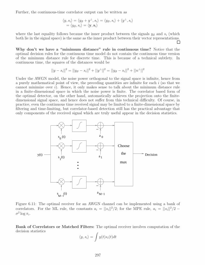
Further, the continuous-time correlator output can be written as

〈y, si〉 = 〈yS + y⊥, si〉 = 〈yS , si〉+ 〈y⊥, si〉= 〈yS , si〉 = 〈y, si〉

where the last equality follows because the inner product between the signals yS and si (whichboth lie in the signal space) is the same as the inner product between their vector representations.

Why don’t we have a “minimum distance” rule in continuous time? Notice that theoptimal decision rules for the continuous time model do not contain the continuous time versionof the minimum distance rule for discrete time. This is because of a technical subtlety. Incontinuous time, the squares of the distances would be

||y − si||2 = ||yS − si||2 + ||y⊥||2 = ||yS − si||2 + ||n⊥||2

Under the AWGN model, the noise power orthogonal to the signal space is infinite, hence froma purely mathematical point of view, the preceding quantities are infinite for each i (so that wecannot minimize over i). Hence, it only makes sense to talk about the minimum distance rulein a finite-dimensional space in which the noise power is finite. The correlator based form ofthe optimal detector, on the other hand, automatically achieves the projection onto the finite-dimensional signal space, and hence does not suffer from this technical difficulty. Of course, inpractice, even the continuous time received signal may be limited to a finite-dimensional space byfiltering and time-limiting, but correlator-based detection still has the practical advantage thatonly components of the received signal which are truly useful appear in the decision statistics.

−

0s (t)

1s (t)

M−1s (t)

a 0

a1

aM−1

y(t) the

Choose

max

Decision

−

−

Figure 6.11: The optimal receiver for an AWGN channel can be implemented using a bank ofcorrelators. For the ML rule, the constants ai = ||si||2/2; for the MPE rule, ai = ||si||2/2 −σ2 log πi.

Bank of Correlators or Matched Filters: The optimal receiver involves computation of thedecision statistics

〈y, si〉 =∫

y(t)si(t)dt

297

t=0

a 0

a1

aM−1

−

−

−

the

Choose

max

Decision

0s (−t)

1s (−t)

M−1s (−t)

y(t)

t=0

t=0

Figure 6.12: An alternative implementation for the optimal receiver using a bank of matchedfilters. For the ML rule, the constants ai = ||si||2/2; for the MPE rule, ai = ||si||2/2− σ2 log πi.

and can therefore be implemented using a bank of correlators, as shown in Figure 6.11. Ofcourse, any correlation operation can also be implemented using a matched filter, sampled at theappropriate time. Defining si,mf(t) = si(−t) as the impulse response of the filter matched to si,we have

〈y, si〉 =∫

y(t)si(t)dt =

∫

y(t)si,mf(−t)dt = (y ∗ si,mf ) (0)

Figure 6.12 shows an alternative implementation for the optimal receiver using a bank of matchedfilters.

Implementation in complex baseband: We have developed the optimal receiver structuresfor real-valued signals, so that these apply to physical baseband and passband signals. However,recall from Chapter 2 that correlation and filtering in passband, which is what the optimal receiverdoes, can be implemented in complex baseband after downconversion. In particular, for passbandsignals up(t) = uc(t) cos 2πfct − us(t) sin 2πfct and vp(t) = vc(t) cos 2πfct − vs(t) sin 2πfct, theinner product can be written as

〈up, vp〉 =1

2(〈uc, vc〉+ 〈us, vs〉) =

1

2Re〈u, v〉 (6.30)

where u = uc+ jus and v = vc+ jvs are the corresponding complex envelopes. Figure 6.13 showshow a passband correlation can be implemented in complex baseband. Note that we correlate theI component with the I component, and the Q component with the Q component. This is becauseour optimal receiver is based on the assumption of coherent reception: our model assumes thatthe receiver has exact copies of the noiseless transmitted signals. Thus, ideal carrier synchronismis implicitly assumed in this model, so that the I and Q components do not get mixed up as theywould if the receiver’s LO were not synchronized to the incoming carrier.

6.2.5 Geometry of the ML decision rule

The minimum distance interpretation for the ML decision rule implies that the decision regions(in signal space) for M-ary signaling in AWGN are constructed as follows. Interpret the signal

298

LPF

c π−2 sin 2 f t

2 cos 2 f tcπy (t)p

y (t)c

y (t)s

s (t)c

s (t)s

Decision

statistic

y (t)p

s (t)p

Decision

statistic

LPF

Figure 6.13: The passband correlations required by the optimal receiver can be implemented incomplex baseband. Since the I and Q components are lowpass waveforms, correlation with themis an implicit form of lowpass filtering. Thus, the LPFs after the mixers could potentially beeliminated, which is why they are shown within dashed boxes.

is an (n−1) dimensional hyperplane

j

si

ML decision boundary

s

Figure 6.14: The ML decision boundary when testing between si and sj is the perpendicularbisector of the line joining the signal points, which is an (n − 1)-dimensional hyperplane for ann-dimensional signal space.

299

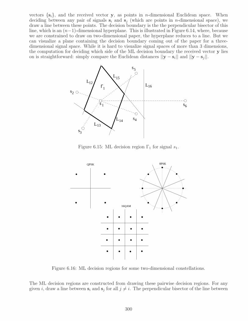
vectors si, and the received vector y, as points in n-dimensional Euclidean space. Whendeciding between any pair of signals si and sj (which are points in n-dimensional space), wedraw a line between these points. The decision boundary is the the perpendicular bisector of thisline, which is an (n−1)-dimensional hyperplane. This is illustrated in Figure 6.14, where, becausewe are constrained to draw on two-dimensional paper, the hyperplane reduces to a line. But wecan visualize a plane containing the decision boundary coming out of the paper for a three-dimensional signal space. While it is hard to visualize signal spaces of more than 3 dimensions,the computation for deciding which side of the ML decision boundary the received vector y lieson is straightforward: simply compare the Euclidean distances ||y− si|| and ||y− sj ||.

1

s2

s3

s4

s5

s6

L12

L13

L14

L15

L16Γ1

s

Figure 6.15: ML decision region Γ1 for signal s1.

QPSK

16QAM

8PSK

Figure 6.16: ML decision regions for some two-dimensional constellations.

The ML decision regions are constructed from drawing these pairwise decision regions. For anygiven i, draw a line between si and sj for all j 6= i. The perpendicular bisector of the line between

300

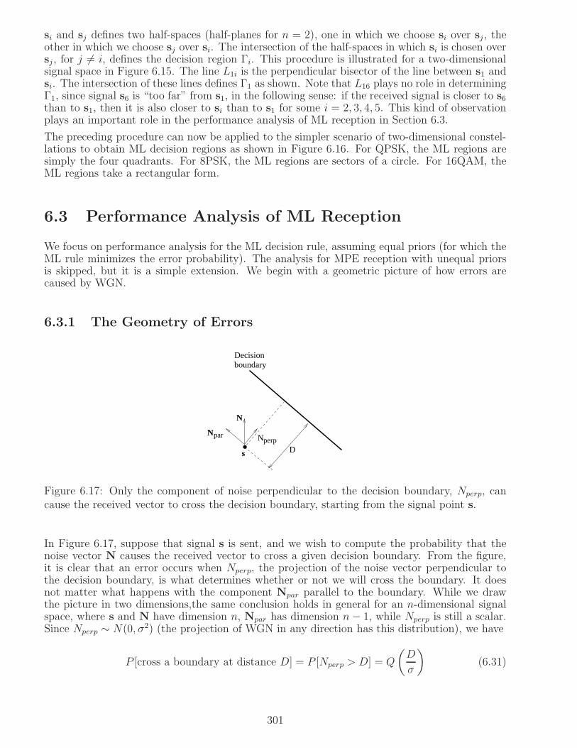
si and sj defines two half-spaces (half-planes for n = 2), one in which we choose si over sj , theother in which we choose sj over si. The intersection of the half-spaces in which si is chosen oversj , for j 6= i, defines the decision region Γi. This procedure is illustrated for a two-dimensionalsignal space in Figure 6.15. The line L1i is the perpendicular bisector of the line between s1 andsi. The intersection of these lines defines Γ1 as shown. Note that L16 plays no role in determiningΓ1, since signal s6 is “too far” from s1, in the following sense: if the received signal is closer to s6than to s1, then it is also closer to si than to s1 for some i = 2, 3, 4, 5. This kind of observationplays an important role in the performance analysis of ML reception in Section 6.3.

The preceding procedure can now be applied to the simpler scenario of two-dimensional constel-lations to obtain ML decision regions as shown in Figure 6.16. For QPSK, the ML regions aresimply the four quadrants. For 8PSK, the ML regions are sectors of a circle. For 16QAM, theML regions take a rectangular form.

6.3 Performance Analysis of ML Reception

We focus on performance analysis for the ML decision rule, assuming equal priors (for which theML rule minimizes the error probability). The analysis for MPE reception with unequal priorsis skipped, but it is a simple extension. We begin with a geometric picture of how errors arecaused by WGN.

6.3.1 The Geometry of Errors

boundary

perpparN

s

N

D

Decision

N

Figure 6.17: Only the component of noise perpendicular to the decision boundary, Nperp, cancause the received vector to cross the decision boundary, starting from the signal point s.

In Figure 6.17, suppose that signal s is sent, and we wish to compute the probability that thenoise vector N causes the received vector to cross a given decision boundary. From the figure,it is clear that an error occurs when Nperp, the projection of the noise vector perpendicular tothe decision boundary, is what determines whether or not we will cross the boundary. It doesnot matter what happens with the component Npar parallel to the boundary. While we drawthe picture in two dimensions,the same conclusion holds in general for an n-dimensional signalspace, where s and N have dimension n, Npar has dimension n− 1, while Nperp is still a scalar.Since Nperp ∼ N(0, σ2) (the projection of WGN in any direction has this distribution), we have

P [cross a boundary at distance D] = P [Nperp > D] = Q

(

D

σ

)

(6.31)

301

boundary

perpparN

1s

1s0

sd=|| − ||0

s

N

D

Decision

N

Figure 6.18: When making an ML decision between s0 and s1, the decision boundary is atdistance D = d/2 from each signal point, where d = ||s1− s0|| is the Euclidean distance betweenthe two points.

Now, let us apply the same reasoning to the decision boundary corresponding to making anML decision between two signals s0 and s1, as shown in Figure 6.18. Suppose that s0 is sent.What is the probability that the noise vector N, when added to it, sends the received vector intothe wrong region by crossing the decision boundary? We know from (6.31) that the answer isQ(D/σ), where D is the distance between s0 and the decision boundary. For ML reception, thedecision boundary is the plane that is the perpendicular bisector of the line between s0 and s1,whose length equals d = ||s1− s0||, the Euclidean distance between the two signal vectors. Thus,D = d/2 = ||s1 − s0||/2. Thus, the probability of crossing the ML decision boundary betweenthe two signal vectors (starting from either of the two signal points) is

P [cross ML boundary between s0 and s1] = Q

( ||s1 − s0||2σ

)

= Q

( ||s1 − s0||2σ

)

(6.32)

where we note that the Euclidean distance between the signal vectors and the correspondingcontinuous time signals is the same.

Notation: Now that we have established the equivalence between working with continuous timesignals and the vectors that represent their projections onto signal space, we no longer need tobe careful about distinguishing between them. Accordingly, we drop the use of boldface notationhenceforth, using the notation y, si and n to denote the received signal, the transmitted signal,and the noise, respectively, in both settings.

6.3.2 Performance with binary signaling

Consider binary signaling in AWGN, where the received signal is modeled using two hypothesesas follows:

H1 : y(t) = s1(t) + n(t)H0 : y(t) = s0(t) + n(t)

(6.33)

Geometric computation of error probability: The ML decision boundary for this problemis as in Figure 6.18. The conditional error probability is simply the probability that, starting fromone of the signal points, the noise makes us cross the boundary to the wrong side, the probabilityof which we have already computed in (6.32). Since the conditional error probabilities are equal,they also equal the average error probability regardless of the priors. We therefore obtain thefollowing expression.

302

Error probability for binary signaling with ML reception

Pe,ML = Pe|1 = Pe|0 = Q

( ||s1 − s0||2σ

)

= Q

(

d

2σ

)

(6.34)

where d = ||s1 − s0|| is the distance between the two possible received signals.

Algebraic computation: While this geometric computation is intuitively pleasing, it is impor-tant to also master algebraic approaches to computing the probabilities of errors due to WGN.It is easiest to first consider on-off keying.

H1 : y(t) = s(t) + n(t)H0 : y(t) = n(t)

(6.35)

Applying (6.28), we find that the ML rule reduces to

〈y, s〉H1

><H0

||s||22

(6.36)

Setting Z = 〈y, s〉, we wish to compute the conditional error probabilities given by

Pe|1 = P [Z <||s||22

|H1] Pe|0 = P [Z >||s||22

|H0] (6.37)

We have actually already done these computations in Example 5.8.2, but it pays to review themquickly. Note that, conditioned on either hypothesis, Z is a Gaussian random variable. Theconditional mean and variance of Z under H0 are given by

E[Z|H0] = E[〈n, s〉] = 0var(Z|H0) = cov(〈n, s〉, 〈n, s〉) = σ2||s||2

where we have used Theorem 6.2.1, and the fact that n(t) has zero mean. The correspondingcomputation under H1 is as follows:

E[Z|H1] = E[〈s + n, s〉] = ||s||2var(Z|H1) = cov(〈s+ n, s〉, 〈s+ n, s〉)cov(〈n, s〉, 〈n, s〉) = σ2||s||2

noting that covariances do not change upon adding constants. Thus, Z ∼ N(0, v2) under H0 andZ ∼ N(m, v2) under H1, where m = ||s||2 and v2 = σ2||s||2. Substituting in (6.37), it is easy tocheck that

Pe|1 = Pe|0 = Q

( ||s||2σ

)

(6.38)

Going back to the more general binary signaling problem (6.33), the ML rule is given by (6.28)to be

〈y, s1〉 −||s1||22

H1

><H0

〈y, s0〉 −||s0||22

303

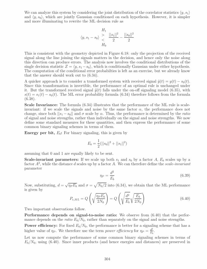
We can analyze this system by considering the joint distribution of the correlator statistics 〈y, s1〉and 〈y, s0〉, which are jointly Gaussian conditioned on each hypothesis. However, it is simplerand more illuminating to rewrite the ML decision rule as

〈y, s1 − s0〉H1

><H0

||s1||22

− ||s0||22

This is consistent with the geometry depicted in Figure 6.18: only the projection of the receivedsignal along the line joining the signals matters in the decision, and hence only the noise alongthis direction can produce errors. The analysis now involves the conditional distributions of thesingle decision statistic Z = 〈y, s1−s0〉, which is conditionally Gaussian under either hypothesis.The computation of the conditional error probabilties is left as an exercise, but we already knowthat the answer should work out to (6.34).

A quicker approach is to consider a transformed system with received signal y(t) = y(t)− s0(t).Since this transformation is invertible, the performance of an optimal rule is unchanged underit. But the transformed received signal y(t) falls under the on-off signaling model (6.35), withs(t) = s1(t)− s0(t). The ML error probability formula (6.34) therefore follows from the formula(6.38).

Scale Invariance: The formula (6.34) illustrates that the performance of the ML rule is scale-invariant: if we scale the signals and noise by the same factor α, the performance does notchange, since both ||s1− s0|| and σ scale by α. Thus, the performance is determined by the ratioof signal and noise strengths, rather than individually on the signal and noise strengths. We nowdefine some standard measures for these quantities, and then express the performance of somecommon binary signaling schemes in terms of them.

Energy per bit, Eb: For binary signaling, this is given by

Eb =1

2(||s0||2 + ||s1||2)

assuming that 0 and 1 are equally likely to be sent.

Scale-invariant parameters: If we scale up both s1 and s0 by a factor A, Eb scales up by afactor A2, while the distance d scales up by a factor A. We can therefore define the scale-invariantparameter

ηP =d2

Eb

(6.39)

Now, substituting, d =√ηPEb and σ =

√

N0/2 into (6.34), we obtain that the ML performanceis given by

Pe,ML = Q

(

√

ηPEb

2N0

)

= Q

(√

d2

Eb

√

Eb

2N0

)

(6.40)

Two important observations follow.

Performance depends on signal-to-noise ratio: We observe from (6.40) that the perfor-mance depends on the ratio Eb/N0, rather than separately on the signal and noise strengths.

Power efficiency: For fixed Eb/N0, the performance is better for a signaling scheme that has a

higher value of ηP . We therefore use the term power efficiency for ηP = d2

Eb.

Let us now compute the performance of some common binary signaling schemes in terms ofEb/N0, using (6.40). Since inner products (and hence energies and distances) are preserved in

304

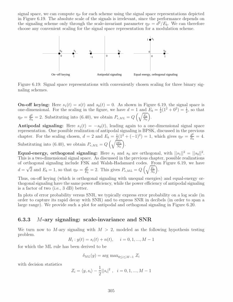
signal space, we can compute ηP for each scheme using the signal space representations depictedin Figure 6.19. The absolute scale of the signals is irrelevant, since the performance depends onthe signaling scheme only through the scale-invariant parameter ηP = d2/Eb. We can thereforechoose any convenient scaling for the signal space representation for a modulation scheme.

0

1

s1 s0 s0s1s0

0 1 1−1

1

0

0

Antipodal signaling Equal energy, orthogonal signalingOn−off keying

1

s

Figure 6.19: Signal space representations with conveniently chosen scaling for three binary sig-naling schemes.

On-off keying: Here s1(t) = s(t) and s0(t) = 0. As shown in Figure 6.19, the signal space isone-dimensional. For the scaling in the figure, we have d = 1 and Eb =

12(12 + 02) = 1

2, so that

ηP = d2

Eb= 2. Substituting into (6.40), we obtain Pe,ML = Q

(√

Eb

N0

)

.

Antipodal signaling: Here s1(t) = −s0(t), leading again to a one-dimensional signal spacerepresentation. One possible realization of antipodal signaling is BPSK, discussed in the previouschapter. For the scaling chosen, d = 2 and Eb =

12(12 + (−1)2) = 1, which gives ηP = d2

Eb= 4.

Substituting into (6.40), we obtain Pe,ML = Q(√

2Eb

N0

)

.

Equal-energy, orthogonal signaling: Here s1 and s0 are orthogonal, with ||s1||2 = ||s0||2.This is a two-dimensional signal space. As discussed in the previous chapter, possible realizationsof orthogonal signaling include FSK and Walsh-Hadamard codes. From Figure 6.19, we have

d =√2 and Eb = 1, so that ηP = d2

Eb= 2. This gives Pe,ML = Q

(√

Eb

N0

)

.

Thus, on-off keying (which is orthogonal signaling with unequal energies) and equal-energy or-thogonal signaling have the same power efficiency, while the power efficiency of antipodal signalingis a factor of two (i.e., 3 dB) better.

In plots of error probability versus SNR, we typically express error probability on a log scale (inorder to capture its rapid decay with SNR) and to express SNR in decibels (in order to span alarge range). We provide such a plot for antipodal and orthogonal signaling in Figure 6.20.

6.3.3 M-ary signaling: scale-invariance and SNR

We turn now to M-ary signaling with M > 2, modeled as the following hypothesis testingproblem.

Hi : y(t) = si(t) + n(t), i = 0, 1, ...,M − 1

for which the ML rule has been derived to be

δML(y) = arg max0≤i≤M−1 Zi

with decision statistics

Zi = 〈y, si〉 −1

2||si|2 , i = 0, 1, ...,M − 1

305

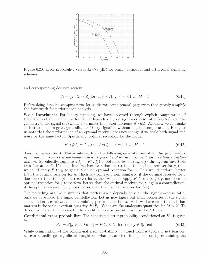
0 2 4 6 8 10 12 14 16 18 2010

−8

10−7

10−6

10−5

10−4

10−3

10−2

10−1

100

Eb/N

o(dB)

Pro

babi

lity

of e

rror

(lo

g sc

ale)

(Orthogonal) FSK/OOK

(Antipodal) BPSK

Figure 6.20: Error probability versus Eb/N0 (dB) for binary antipodal and orthogonal signalingschemes.

and corresponding decision regions

Γi = y : Zi > Zj for all j 6= i , i = 0, 1, ...,M − 1 (6.41)

Before doing detailed computations, let us discuss some general properties that greatly simplifythe framework for performance analysis.

Scale Invariance: For binary signaling, we have observed through explicit computation ofthe error probability that performance depends only on signal-to-noise ratio (Eb/N0) and thegeometry of the signal set (which determines the power efficiency d2/Eb). Actually, we can makesuch statements in great generality for M-ary signaling without explicit computations. First, letus note that the performance of an optimal receiver does not change if we scale both signal andnoise by the same factor. Specifically, optimal reception for the model

Hi : y(t) = Asi(t) + An(t), i = 0, 1, ...,M − 1 (6.42)

does not depend on A. This is inferred from the following general observation: the performanceof an optimal receiver is unchanged when we pass the observation through an invertible transfor-mation. Specifically, suppose z(t) = F (y(t)) is obtained by passing y(t) through an invertibletransformation F . If the optimal receiver for z does better than the optimal receiver for y, thenwe could apply F to y to get z, then do optimal reception for z. This would perform betterthan the optimal receiver for y, which is a contradiction. Similarly, if the optimal receiver for ydoes better than the optimal receiver for z, then we could apply F−1 to z to get y, and then dooptimal reception for y to perform better than the optimal receiver for z, again a contradiction.if the optimal receiver for y does better than the optimal receiver for f(y).

The preceding argument implies that performance depends only on the signal-to-noise ratio,once we have fixed the signal constellation. Let us now figure out what properties of the signalconstellation are relevant in determining performance For M = 2, we have seen that all thatmatters is the scale-invariant quantity d2/Eb. What are the analogous quantities for M > 2? Todetermine these, let us consider the conditional error probabilities for the ML rule.

Conditional error probability: The conditional error probability, conditioned on Hi, is givenby

Pe|i = P [y /∈ Γi|i sent] = P [Zi < Zj for some j 6= i|i sent] (6.43)

While computation of the conditional error probability in closed form is typically not feasible,we can actually get significant insight on what parameters it depends on by examining the

306

conditional distributions of the decision statistics. Since y = si + n conditioned on Hi, thedecision statistics are given by

Zj = 〈y, sj〉 − ||sj||2/2 = 〈si + n, sj〉 − ||sj||2/2 = 〈n, sj〉+ 〈si, sj〉 − ||sj||2/2 , 0 ≤ j ≤M − 1

By the Gaussianity of n(t), the decision statistics Zj are jointly Gaussian (conditioned on Hi).Their joint distribution is therefore completely characterized by their means and covariances.Since the noise is zero mean, we obtain

E[Zj |Hi] = 〈si, sj〉Using Theorem 6.2.1, and noting that covariance is unaffected by translation, we obtain that

cov(Zj, Zk|Hi) = cov (〈n, sj〉, 〈n, sk〉) = σ2〈sj, sk〉Thus, conditioned on Hi, the joint distribution of Zj depends only on the noise variance σ2

and the signal inner products 〈si, sj〉, 1 ≤ i, j ≤M. Now that we know the joint distribution,we can in principle compute the conditional error probabilities Pe|i. In practice, this is oftendifficult, and we often resort to Monte Carlo simulations. However, what we have found outabout the joint distribution can now be used to refine our concepts of scale-invariance.

Performance only depends on normalized inner products: Let us replace Zj by Zj/σ2.

Clearly, since we are simply picking the maximum among the decision statistics, scaling by acommon factor does not change the decision (and hence the performance). However, we nowobtain that

E[Zj

σ2|Hi] =

〈si, sj〉σ2

and

cov

(

Zj

σ2,Zk

σ2|Hi

)

=1

σ4cov(Zj, Zk|Hi) =

〈sj, sk〉σ2

Thus, the joint distribution of the normalized decision statistics Zj/σ2, conditioned on any

of the hypotheses, depends only on the normalized inner products 〈si,sj〉σ2 , 1 ≤ i, j ≤ M. Of

course, this means that the performance also depends only on these normalized inner products.

Let us now carry these arguments further, still without any explicit computations. We defineenergy per symbol and energy per bit for M-ary signaling as follows.

Energy per symbol, Es: For M-ary signaling with equal priors, the energy per symbol Es isgiven by

Es =1

M

M∑

i=1

||si||2

Energy per bit, Eb: Since M-ary signaling conveys log2M bits/symbol, the energy per bit isgiven by

Eb =Es

log2M

If all signals in a M-ary constellation are scaled up by a factor A, then Es and Eb get scaledup by A2, as do all inner products 〈si, sj〉. Thus, we can define scale-invariant inner products

〈si,sj〉Eb

which depend only on the shape of the signal constellation. Indeed, we can define the

shape of a constellation as these scale-invariant inner products. Setting σ2 = N0/2, we can nowwrite the normalized inner products determining performance as follows:

〈si, sj〉σ2

=〈si, sj〉Eb

2Eb

N0(6.44)

307

We can now make the following statement.

Performance depends only on Eb/N0 and constellation shape (as specified by thescale-invariant inner products): We have shown that the performance depends only on the

normalized inner products 〈si,sj〉σ2 . From (6.44), we see that these in turn depend only on Eb/N0

and the scale-invariant inner products

〈si,sj〉Eb

. The latter depend only on the shape of the

signal constellation, and are completely independent of the signal and noise strengths. Whatthis means is that we can choose any convenient scaling that we want for the signal constellationwhen investigating its performance, as long as we keep track of the signal-to-noise ratio. Weillustrate this via an example where we determine the error probability by simulation.

Example 6.3.1 (Using scale-invariance in error probability simulations): Suppose thatwe wish to estimate the error probability for 8PSK by simulation. The signal points lie in a 2-dimensional space, and we can scale them to lie on a circle of unit radius, so that the constellationis given by A = (cos θ, sin θ)T : θ = kπ/4, k = 0, 1, ..., 7. The energy per symbol Es = 1 forthis scaling, so that Eb = Es/ log2 8 = 1/3. We therefore have Eb/N0 = 1/(3N0) = 1/(6σ2), sothat the noise variance per dimension can be set to

σ2 =1

6(Eb/N0)

Typically, Eb/N0 is specified in dB, so we need to convert it to the “raw” Eb/N0. We now havea simulation consisting of the following steps, repeated over multiple symbol transmissions:Step 1: Choose a symbol s at random from A. For this symmetric constellation, we can actuallykeep sending the same symbol in order to compute the performance of the ML rule, since theconditional error probabilities are all equal. For example, set s = (1, 0)T .Step 2: Generate two i.i.d. N(0, 1) random variables Uc and Us. The I and Q noises can now beset as Nc = σUc and Ns = σUs, so that N = (Nc, Ns)

T .Step 3: Set the received vector y = s +N.Step 4: Compute the ML decision arg maxi 〈y, si〉 (the energy terms can be dropped, since thesignals are of equal energy) or arg mini ||y− si||2.Step 5: If there is an error, increment the error count.The error probability is estimated as the error count, divided by the number of symbols trans-mitted. We repeat this simulation over a range of Eb/N0, and typically plot the error probabilityon a log scale versus Eb/N0 in dB.

These steps are carried out in the following code fragment, which generates Figure 6.21 comparinga simulation-based estimate of the error probability for 8PSK against the intelligent union bound,an analytical estimate that we develop shortly. The analytical estimate requires very littlecomputation (evaluation of a single Q function), but its agreement with simulations is excellent.As we shall see, developing such analytical estimates also gives us insight into how errors aremost likely to occur for M-ary signaling in AWGN.

The code fragment is written for transparency rather than computational efficiency. The codecontains an outer for-loop for varying SNR, and an inner for-loop for computing minimum dis-tances for the symbols sent at each SNR. The inner loop can be avoided and the program sped upconsiderably by computing all minimum distances for all symbols at once using matrix operations(try it!). We use a less efficient program here to make the operations easy to understand.

Code Fragment 6.3.1 (Simulation of 8PSK performance in AWGN)

%generate 8PSK constellation as complex numbers

308

0 1 2 3 4 5 6 7 8 9 1010

−3

10−2

10−1

100

Eb/N0 (dB)

Sym

bol e

rror

pro

babi

lity

SimulationIntelligent Union Bound

Figure 6.21: Error probability for 8PSK.

a=cumsum(ones(8,1))-1;constellation = exp(i*2*pi.*a/8);%number of symbols in simulationnsymbols = 20000;ebnodb = 0:0.1:10;number_snrs = length(ebnodb);perr_estimate = zeros(number_snrs,1);for k=1:number_snrs, %SNR for loopebnodb_now = ebnodb(k);ebno=10^(ebnodb_now/10);sigma=sqrt(1/(6*ebno));%send first symbol without loss of generality, add 2d Gaussian noisereceived = 1 + sigma*randn(nsymbols,1)+j*sigma*randn(nsymbols,1);decisions=zeros(nsymbols,1);for n=1:nsymbols, %Symbol for loop (can/should be avoided for fast implementation)

distances = abs(received(n)-constellation);[min_dist,decisions(n)] = min(distances);

enderrors = (decisions ~= 1);perr_estimate(k) = sum(errors)/nsymbols;endsemilogy(ebnodb,perr_estimate);hold on;%COMPARE WITH INTELLIGENT UNION BOUNDetaP = 6-3*sqrt(2); %power efficiencyNdmin = 2;% number of nearest neighborsebno = 10.^(ebnodb/10);perr_union = Ndmin*q_function(sqrt(etaP*ebno/2));semilogy(ebnodb,perr_union,’:r’);xlabel(’Eb/N0 (dB)’);ylabel(’Symbol error probability’);legend(’Simulation’,’Intelligent Union Bound’,’Location’,’NorthEast’);

309

6.3.4 Performance analysis for M-ary signaling

We begin by computing the error probability for QPSK, for which we can get simple expressionsfor the error probability in terms of the Q function. We then discuss why exact performance anal-ysis can be more complicated in general, motivating the need for the bounds and approximationswe develop in this section.

d

01s

s3 s2

Nc

Ns

s

Figure 6.22: If s0 is sent, an error occurs if Nc or Ns is negative enough to make the receivedvector fall out of the first quadrant.

Exact analysis for QPSK: Let us find Pe|0, the conditional error probability for the ML ruleconditioned on s0 being sent. For the scaling shown in Figure 6.22,

s0 =

(

d2d2

)

and the two-dimensional received vector is given by

y = s0 + (Nc, Ns)T =

(

d2+Nc

d2+Ns

)

where Nc, Ns are i.i.d. N(0, σ2) random variables, corresponding to the projections of WGNalong the I and Q axes, respectively. An error occurs if the noise moves the observation outof the positive quadrant, which is the decision region for s0. This happens if Nc +

d2< 0 or

Ns +d2< 0. We can therefore write

Pe|0 = P [Nc+d

2< 0 orNs+

d

2< 0] = P [Nc+

d

2< 0]+P [Ns+

d

2< 0]−P [Nc+

d

2< 0 andNs+

d

2< 0]

(6.45)But

P [Nc +d

2< 0] = P [Nc < −d

2] = Φ

(

− d

2σ

)

= Q

(

d

2σ

)

This is also equal to P [Ns +d2< 0], since Nc, Ns are identically distributed. Furthermore, since

Nc, Ns are independent, we have

P [Nc +d

2< 0 and Ns +

d

2< 0] = P [Nc +

d

2< 0]P [Ns +

d

2< 0] =

[

Q

(

d

2σ

)]2

Substituting these expressions into (6.45), we obtain that

Pe|1 = 2Q

(

d

2σ

)

−Q2

(

d

2σ

)

(6.46)

310

By symmetry, the conditional probabilities Pe|i are equal for all i, which implies that the averageerror probability is also given by the expression above. We now express the error probability interms of the scale-invariant parameter d2

Eband Eb/N0, using the relation

d

2σ=

√

d2

Eb

√

Eb

2N0

The energy per symbol is given by

Es =1

M

M∑

i=1

||si||2 = ||s1||2 =(

d

2

)2

+

(

d

2

)2

=d2

2

which implies that the energy per bit is

Eb =Es

log2M=

Es

log2 4=d2

4

This yields d2

Eb= 4, and hence d

2σ=√

2Eb

N0. Substituting into (6.46), we obtain

Pe = Pe|1 = 2Q

(

√

2Eb

N0

)

−Q2

(

√

2Eb

N0

)

(6.47)

as the exact error probability for QPSK.

0

s2

s3

1N2N

3N

Γ0

s1 s4

s

Figure 6.23: The noise random variables N1, N2, N3 which can drive the received vector outsidethe decision region Γ0 are correlated, which makes it difficult to find an exact expression for Pe|0.

Why exact analysis can be difficult: Let us first understand why we could find a simpleexpression for the error probability for QPSK. The decision regions are bounded by the I andQ axes. The noise random variable Nc can cause crossing of the Q axis, while Ns can causecrossing of the I axis. Since these two random variables are independent, the probability that atleast one of these noise random variables causes a boundary crossing becomes easy to compute.Figure 6.23 shows an example where this is not possible. In the figure, we see that the decision

311

region Γ0 is bounded by three lines (in general, these would be n − 1-dimensional hyperplanesin n-dimensional signal space). An error occurs if we cross any of these lines, starting from s0.In order to cross the line between s0 and si, the noise random variable Ni must be bigger than||si− s0||/2, i = 1, 2, 3 (as we saw in Figures 6.17 and 6.18, only the noise component orthogonalto a hyperplane determines whether we cross it). Thus, the conditional error probability can bewritten as

Pe|0 = P [N1 > ||s1 − s0||/2 or N2 > ||s2 − s0||/2 or N3 > ||s3 − s0||/2] (6.48)

The random variables N1, N2, N3 are, of course, jointly Gaussian, since each is a projectionof WGN along a direction. Each of them is an N(0, σ2) random variable; that is, they areidentically distributed. However, they are not independent, since they are projections of WGNalong directions that are not orthogonal to each other. Thus, we cannot break down the precedingexpression into probabilities in terms of the individual random variables N1, N2, N3, unlike whatwe did for QPSK (where Nc, Ns were independent). However, we can still find a simple upperbound on the conditional error probability using the union bound, as follows.

Union Bound: The probability of a union of events is upper bounded by the sum of theprobabilities of the events.

P [A1 or A2 or ... or An] = P [A1 ∪A2... ∪ An] ≤ P [A1] + P [A2] + ... + P [An] (6.49)

Applying (6.49) to (6.48), we obtain that, for the scenario depicted in Figure 6.23, the conditionalerror probability can be upper bounded as follows:

Pe|0 ≤ P [N1 > ||s1 − s0||/2] + P [N2 > ||s2 − s0||/2] + P [N3 > ||s3 − s0||/2]= Q

(

||s1−s0||2σ

)

+Q(

||s2−s0||2σ

)

+Q(

||s3−s0||2σ

)

(6.50)

Thus, the conditional error probability is upper bounded by a sum of probabilities, each of whichcorresponds to the error probability for a binary decision: s0 versus s1, s0 versus s2, and s0 versuss3. This approach applies in great generality, as we show next.

Union Bound and variants: Pictures such as the one in Figure 6.23 typically cannot bedrawn when the signal space dimension is high. However, we can still find union bounds on errorprobabilities, as long as we can enumerate all the signals in the constellation. To do this, let usrewrite (6.43), the conditional error probability, conditioned on Hi, as a union of M − 1 eventsas follows:

Pe|i = P [∪j 6=iZi < Zj|i sent]]where Zj are the decision statistics. Using the union bound (6.49), we obtain

Pe|i ≤∑

j 6=i

P [Zi < Zj|i sent]] (6.51)

But the jth term on the right-hand side above is simply the error probability of ML receptionfor binary hypothesis testing between the signals si and sj. From the results of Section 6.3.2, wetherefore obtain the following pairwise error probability:

P [Zi < Zj |i sent]] = Q

( ||sj − si||2σ

)

Substituting into (6.51), we obtain upper bounds on the conditional error probabilities and theaverage error probability as follows.

312

Union Bound on conditional error probabilities: The conditional error proba-bilities for the ML rule are bounded as

Pe|i ≤∑

j 6=i

Q

( ||sj − si||2σ

)

=∑

j 6=i

Q

(

dij2σ

)

(6.52)

where dij = ||si − sj|| is the distance between signals si and sj .Union bound on average error probability: Averaging the conditional error usingthe prior probabilities gives an upper bound on the average error probability as follows:

Pe =∑

i

πiPe|i ≤∑

i

πi∑

j 6=i

Q

( ||sj − si||2σ

)

=∑

i

πi∑

j 6=i

Q

(

dij2σ

)

(6.53)

We can now rewrite the union bound in terms of Eb/N0 and the scale-invariant squared

distancesd2ijEb

as follows:

Pe|i ≤∑

j 6=i

Q

√

d2ijEb

√

Eb

2N0

(6.54)

Pe =∑

i

πiPe|i ≤∑

i

πi∑

j 6=i

Q

√

d2ijEb

√

Eb

2N0

(6.55)

Applying the union bound to Figure 6.23, we obtain

Pe|0 ≤ Q

( ||s1 − s0||2σ

)

+Q

( ||s2 − s0||2σ

)

+Q

( ||s3 − s0||2σ

)

+Q

( ||s4 − s0||2σ

)

Notice that this answer is different from the one we had in (6.50). This is because the fourthterm corresponds to the signal s4, which is “too far away” from s0 to play a role in determiningthe decision region Γ0. Thus, when we do have a more detailed geometric understanding of thedecision regions, we can do better than the generic union bound (6.52) and get a tighter bound,as in (6.50). We term this the intelligent union bound, and give a general formulation in thefollowing.

Denote by Nml(i) the indices of the set of neighbors of signal si (we exclude i from Nml(i) bydefinition) that characterize the ML decision region Γi. That is, the half-planes that we intersectto obtain Γi correspond to the perpendicular bisectors of lines joining si and sj , j ∈Nml(i). Forexample, in Figure 6.23, Nml(0) = 1, 2, 3; s4 is excluded from this set, since it does not play arole in determining Γ0. The decision region in (6.41) can now be expressed as

Γi = y : δML(y) = i = y : Zi ≥ Zj for all j ∈Nml(i) (6.56)

We can now say the following: y falls outside Γi if and only if Zi < Zj for some j ∈Nml(i). Wecan therefore write

Pe|i = P [y /∈ Γi|i sent] = P [Zi < Zj for some j ∈Nml(i)|i sent] (6.57)

and from there, following the same steps as in the union bound, get a tighter bound, which weexpress as follows.

313

Intelligent Union Bound: A better bound on Pe|i is obtained by considering onlythe neighbors of si that determine its ML decision region, as follows:

Pe|i ≤∑

j ∈Nml(i)

Q

( ||sj − si||2σ

)

(6.58)

In terms of Eb/N0, we get

Pe|i ≤∑

j ∈Nml(i)

Q

√

d2ijEb

√

Eb

2N0

(6.59)

(the bound on the average error probability Pe is computed as before by averaging thebounds on Pe|i using the priors).

Union Bound for QPSK: For QPSK, we infer from Figure 6.22 that the union bound for Pe|1is given by

Pe = Pe|0 ≤ Q

(

d012σ

)

+Q

(

d022σ

)

+Q

(

d032σ

)

= 2Q

(

d

2σ

)

+Q

(√2d

2σ

)

Using d2

Eb= 4, we obtain the union bound in terms of Eb/N0 to be

Pe ≤ 2Q

(

√

2Eb

N0

)

+Q

(

√

4Eb

N0

)

QPSK union bound (6.60)

For moderately large Eb/N0, the dominant term in terms of the decay of the error probability isthe first one, since Q(x) falls off rapidly as x gets large. Thus, while the union bound (6.60) islarger than the exact error probability (6.47), as it must be, it gets the multiplicity and argumentof the dominant term right. Tightening the analysis using the intelligent union bound, we get

Pe|0 ≤ Q

(

d012σ

)

+Q

(

d022σ

)

= 2Q

(

√

2Eb

N0

)

QPSK intelligent union bound (6.61)

since Nml(0) = 1, 2 (the decision region for s0 is determined by the neighbors s1 and s2).

Another common approach for getting a better (and quicker to compute) estimate than theoriginal union bound is the nearest neighbors approximation. This is a loose term employed todescribe a number of different methods for pruning the terms in the summation (6.52). Mostcommonly, it refers to regular signal sets in which each signal point has a number of nearestneighbors at distance dmin from it, where dmin = mini 6=j ||si − sj||. Letting Ndmin

(i) denote thenumber of nearest neighbors of si, we obtain the following approximation.

Nearest Neighbors Approximation

Pe|i ≈ Ndmin(i)Q

(

dmin

2σ

)

(6.62)

Averaging over i, we obtain that

Pe ≈ NdminQ

(

dmin

2σ

)

(6.63)

314

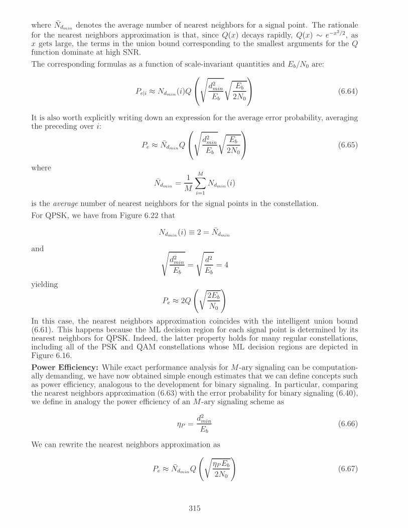
where Ndmindenotes the average number of nearest neighbors for a signal point. The rationale

for the nearest neighbors approximation is that, since Q(x) decays rapidly, Q(x) ∼ e−x2/2, asx gets large, the terms in the union bound corresponding to the smallest arguments for the Qfunction dominate at high SNR.

The corresponding formulas as a function of scale-invariant quantities and Eb/N0 are:

Pe|i ≈ Ndmin(i)Q

√

d2min

Eb

√

Eb

2N0

(6.64)

It is also worth explicitly writing down an expression for the average error probability, averagingthe preceding over i:

Pe ≈ NdminQ

√

d2min

Eb

√

Eb

2N0

(6.65)

where

Ndmin=

1

M

M∑

i=1

Ndmin(i)

is the average number of nearest neighbors for the signal points in the constellation.

For QPSK, we have from Figure 6.22 that

Ndmin(i) ≡ 2 = Ndmin

and√

d2min

Eb

=

√

d2

Eb

= 4

yielding

Pe ≈ 2Q

(

√

2Eb

N0

)

In this case, the nearest neighbors approximation coincides with the intelligent union bound(6.61). This happens because the ML decision region for each signal point is determined by itsnearest neighbors for QPSK. Indeed, the latter property holds for many regular constellations,including all of the PSK and QAM constellations whose ML decision regions are depicted inFigure 6.16.

Power Efficiency: While exact performance analysis for M-ary signaling can be computation-ally demanding, we have now obtained simple enough estimates that we can define concepts suchas power efficiency, analogous to the development for binary signaling. In particular, comparingthe nearest neighbors approximation (6.63) with the error probability for binary signaling (6.40),we define in analogy the power efficiency of an M-ary signaling scheme as

ηP =d2min

Eb(6.66)

We can rewrite the nearest neighbors approximation as

Pe ≈ NdminQ

(

√

ηPEb

2N0

)

(6.67)

315

−1 1 3−3

3

1

−3

−1

Figure 6.24: ML decision regions for 16QAM with scaling chosen for convenience in computingpower efficiency.

Since the argument of the Q function in (6.67) plays a bigger role than the multiplicity Ndminfor

moderately large SNR, ηP offers a means of quickly comparing the power efficiency of differentsignaling constellations, as well as for determining the dependence of performance on Eb/N0.

Performance analysis for 16QAM: We now apply the preceding performance analysis to the16QAM constellation depicted in Figure 6.24, where we have chosen a convenient scale for theconstellation. We now compute the nearest neighbors approximation, which coincides with theintelligent union bound, since the ML decision regions are determined by the nearest neighbors.Noting that the number of nearest neighbors is four for the four innermost signal points, two forthe four outermost signal points, and three for the remaining eight signal points, we obtain uponaveraging

Ndmin= 3 (6.68)

It remains to compute the power efficiency ηP and apply (6.67). We had done this in the previewin Chapter 4, but we repeat it here. For the scaling shown, we have dmin = 2. The energy persymbol is obtained as follows:

Es = average energy of I component + average energy of Q component= 2(average energy of I component)

by symmetry. Since the I component is equally likely to take the four values ±1 and ±3, we have

average energy of I component =1

2(12 + 32) = 5

andEs = 10

We therefore obtain

Eb =Es

log2M=

10

log2 16=

5

2

The power efficiency is therefore given by

ηP =d2min

Eb

=22

52

=8

5(6.69)

Substituting (6.68) and (6.69) into (6.67), we obtain that

Pe(16QAM) ≈ 3Q

(

√

4Eb

5N0

)

(6.70)

316

as the nearest neighbors approximation and intelligent union bound for 16QAM. The bandwidthefficiency for 16QAM is 4 bits/2 dimensions, which is twice that of QPSK, whose bandwidthefficiency is 2 bits/2 dimensions. It is not surprising, therefore, that the power efficiency of16QAM (ηP = 1.6) is smaller than that of QPSK (ηP = 4). We often encounter such tradeoffsbetween power and bandwidth efficiency in the design of communication systems, including whenthe signaling waveforms considered are sophisticated codes that are constructed from multiplesymbols drawn from constellations such as PSK and QAM.

0 2 4 6 8 10 1210

−8

10−7

10−6

10−5

10−4

10−3

10−2

10−1

100

Eb/N0 (dB)

Sym

bol E

rror

Pro

babi

lity

QPSK (IUB)QPSK (exact)16QAM (IUB)16QAM (exact)

Figure 6.25: Symbol error probabilities for QPSK and 16QAM.

Figure 6.25 shows the symbol error probabilities for QPSK and 16QAM, comparing the intelligentunion bounds (which coincide with nearest neighbors approximations) with exact results. Theexact computations for 16QAM use the closed form expression (6.70) derived in Problem 6.21. Wesee that the exact error probability and intelligent union bound are virtually indistinguishable.The power efficiencies of the constellations (which depend on the argument of the Q function)

accurately predict the distance between the curves: ηP (QPSK)ηP (16QAM)

= 41.6

, which equals about 4 dB.

From Figure 6.25, we see that the distance between the QPSK and 16QAM curves at small errorprobabilities (high SNR) is indeed about 4 dB.

D

0

s1

Decision boundary

θ

1 s

Figure 6.26: Performance analysis for BPSK with phase offset.

The performance analysis techniques developed here can also be applied to suboptimal receivers.Suppose, for example, that the receiver LO in a BPSK system is offset from the incoming carrier

317

by a phase shift θ, but that the receiver uses decision regions corresponding to no phase offset.The signal space picture is now as in Figure 6.26. The error probability is now given by

Pe = Pe|0 = Pe|1 = Q

(

D

σ

)

= Q

(√

D2

Eb

2Eb

N0

)

For the scaling shown, D = cos θ and Eb = 1, which gives

Pe = Q

(

√

2Eb cos2 θ

N0

)

so that there is a loss of 10 log10 cos2 θ dB in performance due to the phase offset (e.g. θ = 10

leads to a loss of 0.13 dB, while θ = 30 leads to a loss of 1.25 dB).

6.3.5 Performance analysis for M-ary orthogonal modulation

So far, our examples have focused on two-dimensional modulation, which is what we use whenour primary concern is bandwidth efficiency. We now turn our attention to equal energy, M-ary orthogonal signaling, which, as we have mentioned before, lies at the other extreme of thepower-bandwidth tradeoff space: as M → ∞, the power efficiency reaches the highest possiblevalue of any signaling scheme over the AWGN channel, while the bandwidth efficiency tends tozero. The signal space is M-dimensional in this case, but we can actually get expressions forthe probability of error that involve a single integral rather than M-dimensional integrals, byexploiting the orthogonality of the signal constellation.

Let us first quickly derive the union bound. Without loss of generality, take the M orthogonalsignals as unit vectors along theM axes in our signal space. With this scaling, we have ||si||2 ≡ 1,so that Es = 1 and Eb =

1log2 M

. Since the signals are orthogonal, the squared distance between

any two signals is

d2ij = ||si − sj||2 = ||si||2 + ||sj||2 − 2〈si, sj〉 = 2Es = 2 , i 6= j

Thus, dmin ≡ dij (i 6= j) and the power efficiency

ηP =d2min

Eb= 2 log2M

The union bound, intelligent union bound and nearest neighbors approximation all coincide, andwe get

Pe ≡ Pe|i ≤∑

j 6=i

Q

(

dij2σ

)

= (M − 1)Q

√

d2min

Eb

√

Eb

2N0

We now get the following expression in terms of Eb/N0.

Union bound on error probability for M-ary orthogonal signaling

Pe ≤ (M − 1)Q(√

Eb log2 MN0

)

(6.71)

Exact expressions: By symmetry, the error probability equals the conditional error probability,conditioned on any one of the hypotheses; similarly, the probability of correct decision equals

318

the probability of correct decision given any of the hypothesis. Let us therefore condition onhypothesis H0 (i.e., that s0 is sent), so that the received signal y = s0+n. The decision statistics

Zi = 〈s0 + n, si〉 = Esδ0i +Ni , i = 0, 1, ...,M − 1

where Ni = 〈n, si〉 are jointly Gaussian, zero mean, with

cov(Ni, Nj) = σ2〈si, sj〉 = σ2Esδij

Thus, Ni ∼ N(0, σ2Es) are i.i.d. We therefore infer that, conditioned on s0 sent, the Zi areconditionally independent, with Z0 ∼ N(Es, σ

2Es), and Zi ∼ N(0, σ2Es) for i = 1, ...,M − 1.

Let us now express the decision statistics in scale-invariant terms, by replacing Zi byZi

σ√Es. This

gives Z0 ∼ N(m, 1), Z1, ..., ZM−1 ∼ N(0, 1), conditionally independent, where

m =Es

σ√Es

=

√

Es

σ2=√

2Es/N0 =√

2Eb log2M/N0

The conditional probability of correct reception is now given by

Pc|0 = P [Z1 ≤ Z0, ..., ZM−1 ≤ Z0|H0] =∫

P [Z1 ≤ x, ..., ZM−1 ≤ x|Z0 = x,H0]pZ0|H0(x|H0)dx=∫

P [Z1 ≤ x|H0]...P [ZM−1 ≤ x|H0]pZ0|H0(x|H0)dx

where we have used the conditional independence of the Zi. Plugging in the conditionaldistributions, we get the following expression for the probability of correct reception.

Probability of correct reception for M-ary orthogonal signaling

Pc = Pc|i =∫∞−∞[Φ(x)]M−1 1√

2πe−(x−m)2/2 dx (6.72)

where m =√

2Es/N0 =√

2Eb log2M/N0.

The probability of error is, of course, one minus the preceding expression. But for small errorprobabilities, the probability of correct reception is close to one, and it is difficult to get goodestimates of the error probability using (6.72). We therefore develop an expression for the errorprobability that can be directly computed, as follows:

Pe|0 =∑

j 6=0

P [Zj = maxiZi|H0] = (M − 1)P [Z1 = maxiZi|H0]

where we have used symmetry. Now,

P [Z1 = maxiZi|H0] = P [Z0 ≤ Z1, Z2 ≤ Z1, ..., ZM−1 ≤ Z1|H0]=∫

P [Z0 ≤ x, Z2 ≤ x, ..., ZM−1 ≤ x|Z1 = x,H0]pZ1|H0(x|H0)dx

=∫

P [Z0 ≤ x|H0]P [Z2 ≤ x|H0]...P [ZM−1 ≤ x|H0]pZ1|H0(x|H0)dx

Plugging in the conditional distributions, and multiplying byM−1, gives the following expressionfor the error probability.

Probability of error for M-ary orthogonal signaling

Pe = Pe|i = (M − 1)∫∞−∞[Φ(x)]M−2 Φ(x−m) 1√

2πe−x2/2 dx (6.73)

where m =√

2Es

N0=√

2Eb log2 MN0

.

319

−5 0 5 10 15 2010

−6

10−5

10−4

10−3

10−2

10−1

100

Eb/N

o(dB)

Pro

babi

lity

of s

ymbo

l err

or (

log

scal

e)

M = 8

M =16

M = 4

M = 2

−1.6

Figure 6.27: Symbol error probabilities for M-ary orthogonal signaling.

Asymptotics for large M : The error probability for M-ary orthogonal signaling exhibits aninteresting thresholding effect as M gets large:

limM→∞

Pe =

0, Eb

N0> ln 2

1, Eb

N0< ln 2

(6.74)

That is, by letting M get large, we can get arbitrarily reliable performance as long as Eb/N0

exceeds -1.6 dB (ln 2 expressed in dB). This result is derived in one of the problems. Actually, wecan show using the tools of information theory that this is the best we can do over the AWGNchannel in the limit of bandwidth efficiency tending to zero. That is, M-ary orthogonal signalingis asymptotically optimum in terms of power efficiency.

Figure 6.27 shows the probability of symbol error as a function of Eb/N0 for several values ofM .We see that the performance is quite far away from the asymptotic limit of -1.6 dB (also markedon the plot) for the moderate values of M considered. For example, the Eb/N0 required forachieving an error probability of 10−6 for M = 16 is more than 9 dB away from the asymptoticlimit.

6.4 Bit Error Probability

We now know how to design rules for deciding which of M signals (or symbols) has been sent,and how to estimate the performance of these decision rules. Sending one of M signals conveysm = log2M bits, so that a hard decision on one of these signals actually corresponds to harddecisions on m bits. In this section, we discuss how to estimate the bit error probability, or thebit error rate (BER), as it is often called.

QPSK with Gray coding: We begin with the example of QPSK, with the bit mapping shownin Figure 6.28. This bit mapping is an example of a Gray code, in which the bits correspondingto neighboring symbols differ by exactly one bit (since symbol errors are most likely going tooccur by decoding into neighboring decision regions, this reduces the number of bit errors). Letus denote the symbol labels as b[1]b[2] for the transmitted symbol, where b[1] and b[2] each take

values 0 and 1. Letting b[1]b[2] denote the label for the ML symbol decision, the probabilities of

bit error are given by p1 = P [b[1] 6= b[1]] and p2 = P [b[2] 6= b[2]]. The average probability of biterror, which we wish to estimate, is given by pb =

12(p1 + p2). Conditioned on 00 being sent, the

320

01

c

Ns

d

0010

11

N

Figure 6.28: QPSK with Gray coding.

probability of making an error on b[1] is as follows:

P [b[1] = 1|00 sent] = P [ML decision is 10 or 11|00 sent] = P [Nc < −d2] = Q(

d

2σ) = Q

(

√

2Eb

N0

)

where, as before, we have expressed the result in terms of Eb/N0 using the power efficiencyd2

Eb= 4. We also note, by the symmetry of the constellation and the bit map, that the conditional

probability of error of b[1] is the same, regardless of which symbol we condition on. Moreover,exactly the same analysis holds for b[2], except that errors are caused by the noise randomvariable Ns. We therefore obtain that

pb = p1 = p2 = Q

(

√

2Eb

N0

)

(6.75)

The fact that this expression is identical to the bit error probability for binary antipodal signalingis not a coincidence. QPSK with Gray coding can be thought of as two independent BPSKsystems, one signaling along the I component, and the other along the Q component.

Gray coding is particularly useful at low SNR (e.g., for heavily coded systems), where symbolerrors happen more often. For example, in a coded system, we would pass up fewer bit errors tothe decoder for the same number of symbol errors. We define it in general as follows.

Gray Coding: Consider a 2n-ary constellation in which each point is represented by a binarystring b = (b1, ..., bn). The bit assigment is said to be Gray coded if, for any two constellationpoints b and b′ which are nearest neighbors, the bit representations b and b′ differ in exactlyone bit location.

Nearest neighbors approximation for BER with Gray coded constellation: Considerthe ith bit bi in an n-bit Gray code for a regular constellation with minimum distance dmin. Fora Gray code, there is at most one nearest neighbor which differs in the ith bit, and the pairwiseerror probability of decoding to that neighbor is Q

(

dmin

2σ

)

. We therefore have

P (bit error) ≈ Q

(

√

ηPEb

2N0

)

with Gray coding (6.76)

where ηP =d2min

Ebis the power efficiency.

321

−5 0 5 10 15 2010

−12

10−10

10−8

10−6

10−4

10−2

100

Eb/N

o(dB)

Pro

babi

lity

of b

it er

ror

(BE

R)

(log

scal

e)

ExactNearest Neighbor Approximation

16QAM

16PSK

Figure 6.29: BER for 16QAM and 16PSK with Gray coding.

Figure 6.29 shows the BER of 16QAM and 16PSK with Gray coding, comparing the nearestneighbors approximation with exact results (obtained analytically for 16QAM, and by simulationfor 16PSK). The slight pessimism and ease of computation of the nearest neighbors approximationimplies that it is an excellent tool for link design.

Gray coding may not always be possible. Indeed, for an arbitrary set ofM = 2n signals, we maynot understand the geometry well enough to assign a Gray code. In general, a necessary (butnot sufficient) condition for an n-bit Gray code to exist is that the number of nearest neighborsfor any signal point should be at most n.

BER for orthogonal modulation: For M = 2m-ary equal energy, orthogonal modulation,each of the m bits split the signal set into half. By the symmetric geometry of the signal set,any of the M − 1 wrong symbols are equally likely to be chosen, given a symbol error, and M

2of

these will correspond to error in a given bit. We therefore have

P (bit error) =M2

M − 1P (symbol error), BER for M− ary orthogonal signaling (6.77)

Note that Gray coding is out of the question here, since there are only m bits and 2m − 1neighbors, all at the same distance.

6.5 Link Budget Analysis

We have seen now that performance over the AWGN channel depends only on constellation ge-ometry and Eb/N0. In order to design a communication link, however, we must relate Eb/N0 tophysical parameters such as transmit power, transmit and receive antenna gains, range and thequality of the receiver circuitry. Let us first take stock of what we know:(a) Given the bit rate Rb and the signal constellation, we know the symbol rate (or more gen-erally, the number of modulation degrees of freedom required per unit time), and hence theminimum Nyquist bandwidth Bmin. We can then factor in the excess bandwidth a dictatedby implementation considerations to find the bandwidth B = (1 + a)Bmin required. (However,assuming optimal receiver processing, we show below that the excess bandwidth does not affectthe link budget.)(b) Given the constellation and a desired bit error probability, we can infer the Eb/N0 we need

322

to operate at. Since the SNR satisfies SNR = EbRb

N0B, we have

SNRreqd =

(

Eb

N0

)

reqd

Rb

B(6.78)

(c) Given the receiver noise figure F (dB), we can infer the noise power Pn = N0B = N0,nom10F/10B,

and hence the minimum required received signal power is given by

PRX(min) = SNRreqdPn =

(

Eb

N0

)

reqd

Rb

BN0B =

(

Eb

N0

)

reqd

RbN0,nom10F/10 (6.79)

This is called the required receiver sensitivity, and is usually quoted in dBm, as PRX,dBm(min) =10 log10 PRX(min)(mW). Using (5.93), we obtain that

PRX,dBm(min) =

(

Eb

N0

)

reqd,dB

+ 10 log10Rb − 174 + F (6.80)

where Rb is in bits per second. Note that dependence on bandwidth B (and hence on excessbandwidth) cancels out in (6.79), so that the final expression for receiver sensitivity dependsonly on the required Eb/N0 (which depends on the signaling scheme and target BER), the bitrate Rb, and the noise figure F .

Once we know the receiver sensitivity, we need to determine the link parameters (e.g., transmittedpower, choice of antennas, range) such that the receiver actually gets at least that much power,plus a link margin (typically expressed in dB). We illustrate such considerations via the Friisformula for propagation loss in free space, which we can think of as modeling a line-of-sightwireless link. While deriving this formula from basic electromagnetics is beyond our scope here,let us provide some intuition before stating it.

Suppose that a transmitter emits power PTX that radiates uniformly in all directions. The powerper unit area at a distance R from the transmitter is PTX

4πR2 , where we have divided by the areaof a sphere of radius R. The receive antenna may be thought of as providing an effective area,termed the antenna aperture, for catching a portion of this power. (The aperture of an antennais related to its size, but the relation is not usually straightforward.) If we denote the receiveantenna aperture by ARX , the received power is given by

PRX =PTX

4πR2ARX

Now, if the transmitter can direct power selectively in the direction of the receiver rather thanradiating it isotropically, we get

PRX =PTX

4πR2GTXARX (6.81)

where GTX is the transmit antenna’s gain towards the receiver, relative to a hypothetical isotropicradiator. We now have a formula for received power in terms of transmitted power, which dependson the gain of the transmit antenna and the aperture of the receive antenna. We would like toexpress this formula solely in terms of antenna gains or antenna apertures. To do this, we needto relate the gain of an antenna to its aperture. To this end, we state without proof that theaperture of an isotropic antenna is given by A = λ2

4π. Since the gain of an antenna is the ratio

of its aperture to that of an isotropic antenna. This implies that the relation between gain andaperture can be written as

G =A

λ2/(4π)=

4πA

λ2(6.82)

323

Assuming that the aperture A scales up in some fashion with antenna size, this implies that, fora fixed form factor, we can get higher antenna gains as we decrease the carrier wavelength, orincrease the carrier frequency.

Using (6.82) in (6.81), we get two versions of the Friis formula:

Friis formula for free space propagation

PRX = PTX GTX GRXλ2

16π2R2, in terms of antenna gains (6.83)

PRX = PTXATXARX

λ2R2, in terms of antenna apertures (6.84)

where

• GTX , ATX are the gain and aperture, respectively, of the transmit antenna,• GRX , ARX are the gain and aperture, respectively, of the receive antenna,• λ = c

fcis the carrier wavelength (c = 3 × 108 meters/sec, is the speed of light, fc the carrier

frequency),• R is the range (line-of-sight distance between transmitter and receiver).

The first version (6.83) of the Friis formula tells us that, for antennas with fixed gain, we shouldtry to use as low a carrier frequency (as large a wavelength) as possible. On the other hand,the second version tells us that, if we have antennas of a given form factor, then we can getbetter performance as we increase the carrier frequency (decrease the wavelength), assuming ofcourse that we can “point” these antennas accurately at each other. Of course, higher carrierfrequencies also have the disadvantage of incurring more attenuation from impairments such asobstacles, rain, fog. Some of these tradeoffs are explored in the problems.

In order to apply the Friis formula (let us focus on version (6.83) for concreteness) to link budgetanalysis, it is often convenient to take logarithms, converting the multiplications into addition.On a logarithmic scale, antenna gains are expressed in dBi, where GdBi = 10 log10G for anantenna with raw gain G. Expressing powers in dBm, we have

PRX,dBm = PTX,dBm +GTX,dBi +GRX,dBi + 10 log10λ2

16π2R2(6.85)

More generally, we have the link budget equation

PRX,dBm = PTX,dBm +GTX,dBi +GRX,dBi − Lpathloss,dB(R) (6.86)

where Lpathloss,dB(R) is the path loss in dB. For free space propagation, we have from the Friisformula (6.85) that

Lpathloss,dB(R) = 10 log1016π2R2

λ2path loss in dB for free space propagation (6.87)

While the Friis formula is our starting point, the link budget equation (6.86) applies more gen-erally, in that we can substitute other expressions for path loss, depending on the propagationenvironment. For example, for wireless communication in a cluttered environment, the signalpower may decay as 1

R4 rather than the free space decay of 1R2 . A mixture of empirical mea-

surements and statistical modeling is typically used to characterize path loss as a function ofrange for the environments of interest. For example, the design of wireless cellular systems isaccompanied by extensive “measurement campaigns” and modeling. Once we decide on the pathloss formula (Lpathloss,dB(R)) to be used in the design, the transmit power required to attain agiven receiver sensitivity can be determined as a function of range R. Such a path loss formulatypically characterizes an “average” operating environment, around which there might be sig-nificant statistical variations that are not captured by the model used to arrive at the receiver

324

sensitivity For example, the receiver sensitivity for a wireless link may be calculated based on theAWGN channel model, whereas the link may exhibit rapid amplitude variations due to multipathfading, and slower variations due to shadowing (e.g., due to buildings and other obstacles). Evenif fading/shadowing effects are factored into the channel model used to compute BER, and themodel for path loss, the actual environment encountered may be worse than that assumed inthe model. In general, therefore, we add a link margin Lmargin,dB, again expressed in dB, in anattempt to budget for potential performance losses due to unmodeled or unforeseen impairments.The size of the link margin depends, of course, on the confidence of the system designer in themodels used to arrive at the rest of the link budget.

Putting all this together, if PRX,dBm(min) is the desired receiver sensitivity (i.e., the minimumrequired received power), then we compute the transmit power for the link to be

Required transmit power

PTX,dBm = PRX,dBm(min)−GTX,dBi −GRX,dBi + Lpathloss,dB(R) + Lmargin,dB (6.88)

Let us illustrate these concepts using some examples.

Example 6.5.1 Consider again the 5 GHz WLAN link of Example 5.8.1. We wish to utilize a20 MHz channel, using Gray coded QPSK and an excess bandwidth of 33 %. The receiver hasa noise figure of 6 dB.(a) What is the bit rate?(b) What is the receiver sensitivity required to achieve a BER of 10−6?(c) Assuming transmit and receive antenna gains of 2 dBi each, what is the range achieved for100 mW transmit power, using a link margin of 20 dB? Use link budget analysis based on freespace path loss.Solution (a) For bandwidth B and fractional excess bandwidth a, the symbol rate

Rs =1

T=

B

1 + a=

20

1 + 0.33= 15 Msymbols/sec

and the bit rate for an M-ary constellation is

Rb = Rs log2M = 15 Msymbols/sec × 2 bits/symbol = 30 Mbits/sec

(b) BER for QPSK with Gray coding is Q(√

2Eb

N0

)

. For a desired BER of 10−6, we obtain that(

Eb

N0

)

reqd,db≈ 10.2. Plugging in Rb = 30 Mbps and F = 6 dB in (6.80), we obtain that the

required receiver sensitivity is PRX,dBm(min) = −83 dBm.(c) The transmit power is 100 mW, or 20 dBm. Rewriting (6.88), the allowed path loss to attainthe desired sensitivity at the desired link margin is

Lpathloss,dB(R) = PTX,dBm − PRX,dBm(min) +GTX,dBi +GRX,dBi − Lmargin,dB

= 20− (−83) + 2 + 2− 20 = 87 dB(6.89)

We can now invert the formula for free space loss, (6.87), noting that fc = 5 GHz, which impliesλ = c

fc= 0.06 m. We get a range R of 107 meters, which is of the order of the advertised ranges

for WLANs under nominal operating conditions. The range decreases, of course, for higher bitrates using larger constellations. What happens, for example, when we use 16QAM or 64QAM?

Example 6.5.2 Consider an indoor link at 10 meters range using unlicensed spectrum at 60GHz. Suppose that the transmitter and receiver each use antennas with horizontal beamwidths

325

of 60 and vertical beamwidths of 30. Use the following approximation to calculate the resultingantenna gains:

G ≈ 41000

θhorizθvert

where G denotes the antenna gain (linear scale), θhoriz and θvert denote horizontal and verticalbeamwidths (in degrees). Set the noise figure to 8 dB, and assume a link margin of 10 dB atBER of 10−6.(a) Calculate the bandwidth and transmit power required for a 2 Gbps link using Gray codedQPSK and 50% excess bandwidth.(b) How do your answers change if you change the signaling scheme to Gray coded 16QAM,keeping the same bit rate as in (a)?(c) If you now employ Gray coded 16QAM keeping the same symbol rate as in (a), what is thebit rate attained and the transmit power required?(d) How do the answers in the setting of (a) change if you increase the horizontal beamwidth to120, keeping all other parameters fixed?Solution: (a) A 2 Gbps link using QPSK corresponds to a symbol rate of 1 Gsymbols/sec.Factoring in the 50% excess bandwidth, the required bandwidth is B = 1.5 GHz. The targetBER and constellation are as in the previous example, hence we still have (Eb/N0)reqd,dB ≈ 10.2dB. Plugging in Rb = 2 Gbps and F = 8 dB in (6.80), we obtain that the required receiversensitivity is PRX,dBm(min) = −62.8 dBm.The antenna gains at each end are given by

G ≈ 41000

60× 30= 22.78

Converting to dB scale, we obtain GTX,dBi = GRX,dBi = 13.58 dBi.The transmit power for a range of 10 m can now be obtained using (6.88) to be 8.1 dBm.(b) For the same bit rate of 2 Gbps, the symbol rate for 16QAM is 0.5 Gsymbols/sec, so thatthe bandwidth required is 0.75 GHz, factoring in 50% excess bandwidth. The nearest neighbors

approximation to BER for Gray coded 16QAM is given by Q(√

4Eb

5N0

)

. Using this, we find that

a target BER of 10−6 requires (Eb/N0)reqd,dB ≈ 14.54 dB, and increase of 4.34 dB relative to (a).This leads to a corresponding increase in the receiver sensitivity to -58.45 dBm, which leads tothe required transmit power increasing to 12.4 dBm.(c) If we keep the symbol rate fixed at 1 Gsymbols/sec, the bit rate with 16QAM is Rb = 4 Gbps.As in (b), (Eb/N0)reqd,dB ≈ 14.54 dB. The receiver sensitivity is therefore given by -55.45 dBm,a 3 dB increase over (b), corresponding to the doubling of the bit rate. This translates directlyto a 3 dB increase, relative to (b), in transmit power to 15.4 dBm, since the path loss, antennagains, and link margin are as in (b).(d) We now go back to the setting of (a), but with different antenna gains. The bandwidth is,of course, unchanged from (a). The new antenna gains are 3 dB smaller because of the doublingof horizontal beamwidth. The receiver sensitivity, path loss and link margin are as in (a), thusthe 3 dB reduction in antenna gains at each end must be compensated for by a 6 dB increase intransmit power relative to (a). Thus, the required transmit power is 14.1 dBm.

Discussion: The parameter choices in the preceding examples illustrate how physical character-istics of the medium change with choice of carrier frequency, and affect system design tradeoffs.The 5 GHz system in Example 6.5.1 employs essentially omnidirectional antennas with smallgains of 2 dBi, whereas it is possible to realize highly directional yet small antennas (e.g., usingelectronically steerable printed circuit antenna arrays) for the 60 GHz system in Example 6.5.2by virtue of the small (5 mm) wavelength. 60 GHz waves are easily blocked by walls, hence therange in Example 6.5.2 corresponds to in-room communication. We have also chosen parameterssuch that the transmit power required for 60 GHz is smaller than that at 5 GHz, since it is

326

more difficult to produce power at higher radio frequencies. Finally, the link margin for 5 GHzis chosen higher than for 60 GHz: propagation at 60 GHz is near line-of-sight, whereas fadingdue to multipath propagation at 5 GHz can be more significant, and hence may require a higherlink margin relative to the AWGN benchmark which provides the basis for our link budget.


This chapter establishes a systematic hypothesis testing based framework for demodulation, de-velops tools for performance evaluation which enable exploration of the power-bandwidth trade-offs exhibited different signaling schemes, and relates these mathematical models to physical linkparameters via the link budget. A summary of some key concepts and results is as follows.

Hypothesis testing• The probability of error is minimized by choosing the hypothesis with the maximum a posterioriprobability (i.e., the hypothesis that is most likely conditioned on the observation). That is, theMPE rule is also the MAP rule:

δMPE(y) = δMAP (y) = arg max1≤i≤M P [Hi|Y = y]= arg max1≤i≤M πip(y|i) = arg max1≤i≤M log πi + log p(y|i)

For equal priors, the MPE rule coincides with the ML rule:

δML(y) = arg max1≤i≤M p(y|i) = arg max1≤i≤M log p(y|i)

• For binary hypothesis testing, ML and MPE rules can be written as likelihood, or log likelihood,ratio tests:

L(y) =p1(y)

p0(y)

H1

><H0

1 or logL(y)

H1

><H0

0 ML rule

L(y) =p1(y)

p0(y)

H1

><H0

π0π1

or logL(y)

H1

><H0

π0π1

MPE/MAP rule

Geometric view of signalsContinuous-time signals can be interpreted as vectors in Euclidean space, with inner product〈s1, s2〉 =

∫

s1(t)s∗2(t) dt, norm ||s|| =

√

〈s, s〉, and energy ||s||2 = 〈s, s〉. Two signals areorthogonal if their inner product is zero.

Geometric view of WGN• WGN n(t) with PSD σ2, when projected in any “direction” (i.e., correlated against any unitenergy signal), yields an N(0, σ2) random variable. • More generally, projections of the noisealong any signals are jointly Gaussian, with zero mean and cov (〈n, u〉, 〈n, v〉) = σ2〈v, u〉.• Noise projections along orthogonal signals are uncorrelated. Since they are jointly Gaussian,they are also independent.

Signal space• M-ary signaling in AWGN in continuous time can be reduced, without loss of information,to M-ary signaling in finite-dimensional vector space with each dimension seeing i.i.d. N(0, σ2)noise, which corresponds to discrete time WGN. This is accomplished by projecting the receivedsignal onto the signal space spanned by the M possible signals.

327

• Decision rules derived using hypothesis testing in the finite-dimensional signal space mapdirectly back to continuous time because of two key reasons: signal inner products are preserved,and the noise component orthogonal to the signal space is irrelevant. Because of this equivalence,we can stop making a distinction between continuous time signals and finite-dimensional vectorsignals in our notation.

Optimal demodulation• For the model Hi = y = si+n, 0 ≤ i ≤M − 1, optimum demodulation involve computation ofthe correlator outputs Zi = 〈y, si〉. This can be accomplished by using a bank of correlators ormatched filters, but any other other receiver structure that yields the statistics Zi would alsopreserve all of the relevant information.• The ML and MPE rules are given by

δML(y) = arg max0≤i≤M−1 〈y, si〉 −||si||22

δMPE(y) = arg max0≤i≤M−1 〈y, si〉 −||si||22

+ σ2 log πi

When the received signal lies in a finite-dimensional space in which the noise has finite energy,the ML rule can be written as a minimum distance rule (and the MPE rule as a variant thereof)as follows:

δML(y)arg min0≤i≤M−1 ||y − si||2δMPE(y) = arg min0≤i≤M−1 ||y − si||2 − 2σ2 log πi

Geometry of ML rule: ML decision boundaries are formed from hyperplanes that bisect linesconnecting signal points.

Performance analysis• For binary signaling, the error probability for the ML rule is given by

Pe = Q

(

d

2σ

)

= Q

(√

d2

Eb

√

Eb

2N0

)

where d = ||s1 − s0|| is the Euclidean distance between the signals. The performance therefore

depends on the power efficiency ηP = d2

Eband the SNR Eb/N0. Since the power efficiency is scale-

invariant, we may choose any convenient scaling when computing it for a given constellation.• For M-ary signaling, closed form expressions for the error probability may not be available,

but we know that the performance depends only on the scale-invariant inner products 〈si,sj〉Eb

,which depend on the constellation “shape” alone, and on Eb/N0.• The conditional error probabilities for M-ary signaling can be bounded using the union bound(these can then be averaged to obtain an upper bound on the average error probability):

Pe|i ≤∑

j 6=i

Q

(

dij2σ

)

=∑

j 6=i

Q

√

d2ijEb

√

Eb

2N0

where dij = ||si − sj|| are the pairwise distances between signal points.• When we understand the shape of the decision regions, we can tighten the union bound intoan intelligent union bound:

Pe|i ≤∑

j ∈Nml(i)

Q

( ||dij||2σ

)

=∑

j ∈Nml(i)

Q

√

d2ijEb

√

Eb

2N0

328

where Nml(i) denotes the set of neighbors of si which define the decision region Γi.• For regular constellations, the nearest neighbors approximation is given by

Pe|i ≈ Ndmin(i)Q

(

dmin

2σ

)

= Ndmin(i)Q

√

d2min

Eb

√

Eb

2N0

Pe ≈ NdminQ

(

dmin

2σ

)

= NdminQ

√

d2min

Eb

√

Eb

2N0

with ηP =d2min

Ebproviding a measure of power efficiency which can be used to compare across

constellations.• If Gray coding is possible, the bit error probability can be estimated as

P (bit error) ≈ Q

(

√

ηPEb

2N0

)

Link budget: This relates (e.g., using the Friis formula for free space propagation) the per-formance of a communication link to physical parameters such as transmit power, transmit andreceive antenna gains, range, and receiver noise figure. A link margin is typically introduced toaccount for unmodeled impairments.

6.7 Endnotes

The geometric signal space approach for deriving and analyzing is now standard in textbookson communication theory, such as [7, 8]. It was first developed by Russian pioneer VladimirKotelnikov [29], and presented in a cohesive fashion in the classic textbook by Wozencraft andJacobs [9].

A number of details of receiver design have been swept under the rug in this chapter. Ourmodel for the received signal is that it equals the transmitted signal plus WGN. In practice,the transmitted signal can be significantly distorted by the channel (e.g., scaling, delay, multi-path propagation). However, the basic M-ary signaling model is still preserved: if M possiblesignals are sent, then, prior to the addition of noise, M possible signals are received after thedeterministic (but a priori unknown) transformations due to channel impairments. The receivercan therefore estimate noiseless copies of the latter and then apply the optimum demodula-tion techniques developed here. This approach leads, for example, to the optimal equalizationstrategies developed by Forney [30] and Ungerboeck [31]; see Chapter 5 of [7] for a textbookexposition. Estimation of the noiseless received signals involves tasks such as carrier phase andfrequency synchronization, timing synchronization, and estimation of the channel impulse re-sponse or transfer function. In modern digital communication transceivers, these operationsare typically all performed using DSP on the complex baseband received signal. Perhaps thebest approach for exploring further is to acquire a basic understanding of the relevant estima-tion techniques, and to then go to technical papers of specific interest (e.g., IEEE conferenceand journal publications). Classic texts covering estimation theory include Kay [32], Poor [33]and Van Trees [34]. Several graduate texts in communications contain a brief discussion of themodern estimation-theoretic approach to synchronization that may provide a helpful orientationprior to going to the research literature; for example, see [7] (Chapter 4) and [11, 35] (Chapter8).

329

Problems

Hypothesis Testing

Problem 6.1 The received signal in a digital communication system is given by

y(t) =

s(t) + n(t) 1 sentn(t) 0 sent

where n is AWGN with PSD σ2 = N0/2 and s(t) is as shown below. The received signal is passed

t = t0

ML decision

ruleh(t)0 2 4

1

-1

t

s(t)

Figure 6.30: Set-up for Problem 6.1

through a filter, and the output is sampled to yield a decision statistic. An ML decision rule isemployed based on the decision statistic. The set-up is shown in Figure 6.30.(a) For h(t) = s(−t), find the error probability as a function of Eb/N0 if t0 = 1.(b) Can the error probability in (a) be improved by choosing the sampling time t0 differently?(c) Now, find the error probability as a function of Eb/N0 for h(t) = I[0,2] and the best possiblechoice of sampling time.(d) Finally, comment on whether you can improve the performance in (c) by using a linear com-bination of two samples as a decision statistic, rather than just using one sample.

Problem 6.2 Consider binary hypothesis testing based on the decision statistic Y , where Y ∼N(2, 9) under H1 and Y ∼ N(−2, 4) under H0.(a) Show that the optimal (ML or MPE) decision rule is equivalent to comparing a function ofthe form ay2 + by to a threshold.(b) Specify the MPE rule explicitly (i.e., specify a, b and the threshold) when π0 =

14.

(c) Express the conditional error probability Pe|0 for the decision rule in (b) in terms of the Qfunction with positive arguments. Also provide a numerical value for this probability.

Problem 6.3 Find and sketch the decision regions for a binary hypothesis testing problem withobservation Z, where the hypotheses are equally likely, and the conditional distributions aregiven byH0: Z is uniform over [−2, 2]H1: Z is Gaussian with mean 0 and variance 1.

Problem 6.4 The receiver in a binary communication system employs a decision statistic Zwhich behaves as follows:Z = N if 0 is sentZ = 4 +N if 1 is sentwhere N is modeled as Laplacian with density

pN(x) =1

2e−|x|, −∞ < x <∞

330

Note: Parts (a) and (b) can be done independently.(a) Find and sketch, as a function of z, the log likelihood ratio

K(z) = logL(z) = logp(z|1)p(z|0)

where p(z|i) denotes the conditional density of Z given that i is sent (i = 0, 1).(b) Find Pe|1, the conditional error probability given that 1 is sent, for the decision rule

δ(z) =

0, z < 11, z ≥ 1

(c) Is the rule in (b) the MPE rule for any choice of prior probabilities? If so, specify the priorprobability π0 = P [ 0 sent] for which it is the MPE rule. If not, say why not.

Problem 6.5 Consider the MAP/MPE rule for the hypothesis testing problem in Example6.1.1.(a) Show that the MAP rule always says H1 if the prior probability of H0 is smaller than somepositive threshold. Specify this threshold.(b) Compute and plot the conditional probabilities Pe|0 and Pe|1, and the average error proba-bility Pe, versus π0 as the latter varies in [0, 1].(c) Discuss any trends that you see from the plots in (b).

Problem 6.6 Consider a MAP receiver for the basic Gaussian example, as discussed in Example6.1.2. Fix SNR at 13 dB. We wish to explore the effect of prior mismatch, by quantifying theperformance degradation of a MAP receiver if the actual priors are different from the priors forwhich it has been designed.(a) Plot the average error probability for a MAP receiver designed for π0 = 0.2, as π0 variesfrom 0 to 1. As usual, use a log scale for the probabilities. On the same plot, also plot the errorprobability of the ML receiver as a benchmark.(b) From the plot in (a), comment on how much error you can tolerate in the prior probabilitiesbefore the performance of the MAP receiver designed for the given prior becomes unacceptable.(c) Repeat (a) and (b) for a MAP receiver designed for π0 = 0.4. Is the performance more orless sensitive to errors in the priors?

Problem 6.7 Consider binary hypothesis testing in which the observation Y is modeled as uni-formly distributed over [−2, 2] underH0, and has conditional density p(y|1) = c(1−|y|/3)I[−3,3](y)under H1, where c > 0 is a constant to be determined.(a) Find c.(b) Find and sketch the decision regions Γ0 and Γ1 corresponding to the ML decision rule.(c) Find the conditional error probabilities.

Problem 6.8 Consider binary hypothesis testing with scalar observation Y . Under hypothesisH0, Y is modeled as uniformly distributed over [−5, 5]. Under H1, Y has conditional densityp(y|1) = 1

8e−|y|/4, −∞ < y <∞.

(a) Specify the ML rule and clearly draw the decision regions Γ0 and Γ1 on the real line.(b) Find the conditional probabilities of error for the ML rule under each hypothesis.

Problem 6.9 For the setting of Problem 6.8, suppose that the prior probability of H0 is 1/3.(a) Specify the MPE rule and draw the decision regions.(b) Find the conditional error probabilities and the average error probability. Compare with thecorresponding quantities for the ML rule considered in Problem 6.8.

331

Problem 6.10 The receiver output Z in an on-off keyed optical communication system is mod-eled as a Poisson random variable with mean m0 = 1 if 0 is sent, and mean m1 = 10 if 1 is sent.(a) Show that the ML rule consists of comparing Z to a threshold, and specify the numericalvalue of the threshold. Note that Z can only take nonnegative integer values.(b) Compute the conditional error probabilities for the ML rule (compute numerical values inaddition to deriving formulas).(c) Find the MPE rule if the prior probability of sending 1 is 0.1.(d) Compute the average error probability for the MPE rule.

Problem 6.11 The received sample Y in a binary communication system is modeled as follows:Y = A +N if 0 is sent, and Y = −A+N if 1 is sent, where N is Laplacian noise with density

pN(x) =λ

2e−λ|x| , −∞ < x <∞

(a) Find the ML decision rule. Simplify as much as possible.(b) Find the conditional error probabilities for the ML rule.(c) Now, suppose that the prior probability of sending 0 is 1/3. Find the MPE rule, simplifyingas much as possible.

(d) In the setting of (c), find the LLR log P [0|Y=A/2]P [1|Y=A/2]

.

Problem 6.12 Consider binary hypothesis testing with scalar observation Y . Under hypothesisH0, Y is modeled as an exponential random variable with mean 5. Under hypothesis H1, Y ismodeled as uniformly distributed over the interval [0, 10].(a) Specify the ML rule and clearly draw the decision regions Γ0 and Γ1 on the real line.(b) Find the conditional probability of error for the ML rule, given that H0 is true.(c) Suppose that the prior probability of H0 is 1/3. Compute the posterior probability of H0

given that we observe Y = 4 (i.e., find P [H0|Y = 4]).

Problem 6.13 Consider hypothesis testing in which the observation Y is given by the followingmodel:

H1 : Y = 6 +NH0 : Y = N

where the noise N has density pN(x) =110

(

1− |x|10

)

I[−10,10](x).

(a) Find the conditional error probability given H1 for the following decision rule:

Y

H1

><H0

4

(b) Are there a set of prior probabilities for which the decision rule in (a) minimizes the errorprobability? If so, specify them. If not, say why not.

Receiver design and performance analysis for the AWGN channel

Problem 6.14 Consider binary signaling in AWGN, with s1(t) = (1 − |t|)I[−1,1](t) and s0(t) =−s1(t). The received signal is given by y(t) = si(t) + n(t), i = 0, 1,, where the noise n has PSDσ2 = N0

2= 0.1. For all of the error probabilities computed in this problem, specify in terms of

332

the Q function with positive arguments and also give numerical values.(a) How would you implement the ML receiver using the received signal y(t)? What is itsconditional error probability given that s0 is sent?Now, consider a suboptimal receiver, where the receiver generates the following decision statistics:

y0 =

∫ −0.5

−1

y(t)dt, y1 =

∫ 0

−0.5

y(t)dt, y2 =

∫ 0.5

0

y(t)dt, y0 =

∫ 1

0.5

y(t)dt

(b) Specify the conditional distribution of y = (y0, y1, y2, y3)T , conditioned on s0 being sent.

(c) Specify the ML rule when the observation is y. What is its conditional error probabilitygiven that s0 is sent?(d) Specify the ML rule when the observation is y0 + y1 + y2 + y3. What is its conditional errorprobability, given that s0 is sent?(e) Among the error probabilities in (a), (c) and (d), which is the smallest? Which is the biggest?Could you have rank ordered these error probabilities without actually computing them?

Problem 6.15 The received signal in an on-off keyed digital communication system is given by

y(t) =

s(t) + n(t) 1 sentn(t) 0 sent

where n is AWGN with PSD σ2 = N0/2, and s(t) = A(1−|t|)I[−1,1](t), where A > 0. The receivedsignal is passed through a filter with impulse response h(t) = I[0,1](t) to obtain z(t) = (y ∗ h)(t).Remark: It would be helpful to draw a picture of the system before you start doing the calculations.(a) Consider the decision statistic Z = z(0) + z(1). Specify the conditional distribution of Zgiven that 0 is sent, and the conditional distribution of Z given that 1 is sent.(b) Assuming that the receiver must make its decision based on Z, specify the ML rule and itserror probability in terms of Eb/N0 (express your answer in terms of the Q function with positivearguments).(c) Find the error probability (in terms of Eb/N0) for ML decisions based on the decision statisticZ2 = z(0) + z(0.5) + z(1).

1

0

s (t)1

−1

3

0 2

1

t

t

s (t)

Figure 6.31: Signal Set for Problem 6.16.

Problem 6.16 Consider binary signaling in AWGN using the signals depicted in Figure 6.31.The received signal is given by

y(t) =

s1(t) + n(t), 1 sents0(t) + n(t), 0 sent

333

where n(t) is WGN with PSD σ2 = N0/2.(a) Show that the ML decision rule can be implemented by comparing Z =

∫

y(t)a(t)dt to athreshold γ. Sketch a(t) and specify the corresponding value of γ.(b) Specify the error probability of the ML rule as a function of Eb/N0.(c) Can the MPE rule, assuming that the prior probability of sending 0 is 1/3, be implementedusing the same receiver structure as in (a)? What would need to change? (Be specific.)(d) Consider now a suboptimal receiver structure in which y(t) is passed through a filter withimpulse response h(t) = I[0,1](t), and we take three samples: Z1 = (y ∗ h)(1), Z2 = (y ∗ h)(2),Z3 = (y ∗ h)(3). Specify the conditional distribution of Z = (Z1, Z2, Z3)

T given that 0 is sent.(e) (more challenging) Specify the ML rule based on Z and the corresponding error probabilityas a function of Eb/N0.

Problem 6.17 Let p1(t) = I[0,1](t) denote a rectangular pulse of unit duration. Consider two4-ary signal sets as follows:Signal Set A: si(t) = p1(t− i), i = 0, 1, 2, 3.Signal Set B: s0(t) = p1(t) + p1(t − 3), s1(t) = p1(t − 1) + p1(t − 2), s2(t) = p1(t) + p1(t − 2),s3(t) = p1(t− 1) + p1(t− 3).(a) Find signal space representations for each signal set with respect to the orthonormal basisp1(t− i), i = 0, 1, 2, 3.(b) Find union bounds on the average error probabilities for both signal sets as a function ofEb/N0. At high SNR, what is the penalty in dB for using signal set B?(c) Find an exact expression for the average error probability for signal set B as a function ofEb/N0.

0

t t

t t

a(t) b(t)

c(t) d(t)

2

−2 −1 0 1 2

−2 −1 0 1 2

−2 −1 0 1 2

−2 −1 1 2

2

−2

2

−2

2

−2

Figure 6.32: Signal Set for Problem 6.18

Problem 6.18 Consider the 4-ary signaling set shown in Figure 6.32, to be used over an AWGNchannel.(a) Find a union bound, as a function of Eb/N0, on the conditional probability of error giventhat c(t) is sent.(b) True or False This constellation is more power efficient than QPSK. Justify your answer.

Problem 6.19 Three 8-ary signal constellations are shown in Figure 6.33.

(a) Express R and d(2)min in terms of d

(1)min so that all three constellations have the same Eb.

(b) For a given Eb/N0, which constellation do you expect to have the smallest bit error probabilityover a high SNR AWGN channel?

334

QAM1 QAM2

R

8-PSK

Figure 6.33: Signal constellations for Problem 6.19

(c) For each constellation, determine whether you can label signal points using 3 bits so that thelabel for nearest neighbors differs by at most one bit. If so, find such a labeling. If not, say whynot and find some “good” labeling.(d) For the labelings found in part (c), compute nearest neighbors approximations for the averagebit error probability as a function of Eb/N0 for each constellation. Evaluate these approximationsfor Eb/N0 = 15dB.

Problem 6.20 Consider the signal constellation shown in Figure 6.34, which consists of twoQPSK constellations of different radii, offset from each other by π

4. The constellation is to be

used to communicate over a passband AWGN channel.

R

r

Figure 6.34: Constellation for Problem 6.20

(a) Carefully redraw the constellation (roughly to scale, to the extent possible) for r = 1 andR =

√2. Sketch the ML decision regions.

(b) For r = 1 and R =√2, find an intelligent union bound for the conditional error probability,

given that a sign al point from the inner circle is sent, as a function of Eb/N0.(c) How would you choose the parameters r and R so as to optimize the power efficiency of theconstellation (at high SNR )?

Problem 6.21 (Exact symbol error probabilities for rectangular constellations) As-suming each symbol is equally likely, derive the following expressions for the average error prob-ability for 4PAM and 16QAM:

335

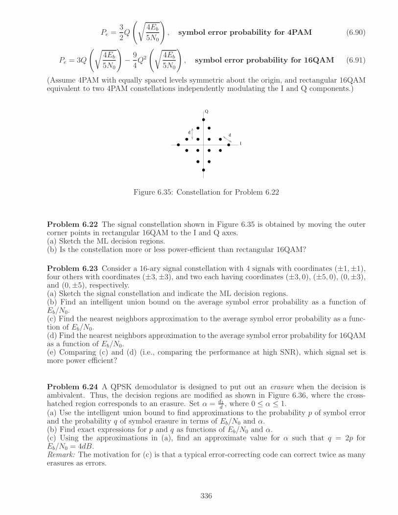
Pe =3

2Q

(

√

4Eb

5N0

)

, symbol error probability for 4PAM (6.90)

Pe = 3Q

(

√

4Eb

5N0

)

− 9

4Q2

(

√

4Eb

5N0

)

, symbol error probability for 16QAM (6.91)

(Assume 4PAM with equally spaced levels symmetric about the origin, and rectangular 16QAMequivalent to two 4PAM constellations independently modulating the I and Q components.)

d

I

Q

d


Problem 6.22 The signal constellation shown in Figure 6.35 is obtained by moving the outercorner points in rectangular 16QAM to the I and Q axes.(a) Sketch the ML decision regions.(b) Is the constellation more or less power-efficient than rectangular 16QAM?

Problem 6.23 Consider a 16-ary signal constellation with 4 signals with coordinates (±1,±1),four others with coordinates (±3,±3), and two each having coordinates (±3, 0), (±5, 0), (0,±3),and (0,±5), respectively.(a) Sketch the signal constellation and indicate the ML decision regions.(b) Find an intelligent union bound on the average symbol error probability as a function ofEb/N0.(c) Find the nearest neighbors approximation to the average symbol error probability as a func-tion of Eb/N0.(d) Find the nearest neighbors approximation to the average symbol error probability for 16QAMas a function of Eb/N0.(e) Comparing (c) and (d) (i.e., comparing the performance at high SNR), which signal set ismore power efficient?

Problem 6.24 A QPSK demodulator is designed to put out an erasure when the decision isambivalent. Thus, the decision regions are modified as shown in Figure 6.36, where the cross-hatched region corresponds to an erasure. Set α = d1

d, where 0 ≤ α ≤ 1.

(a) Use the intelligent union bound to find approximations to the probability p of symbol errorand the probability q of symbol erasure in terms of Eb/N0 and α.(b) Find exact expressions for p and q as functions of Eb/N0 and α.(c) Using the approximations in (a), find an approximate value for α such that q = 2p forEb/N0 = 4dB.Remark: The motivation for (c) is that a typical error-correcting code can correct twice as manyerasures as errors.

336

d

1d

Figure 6.36: QPSK with erasures

Rr


337

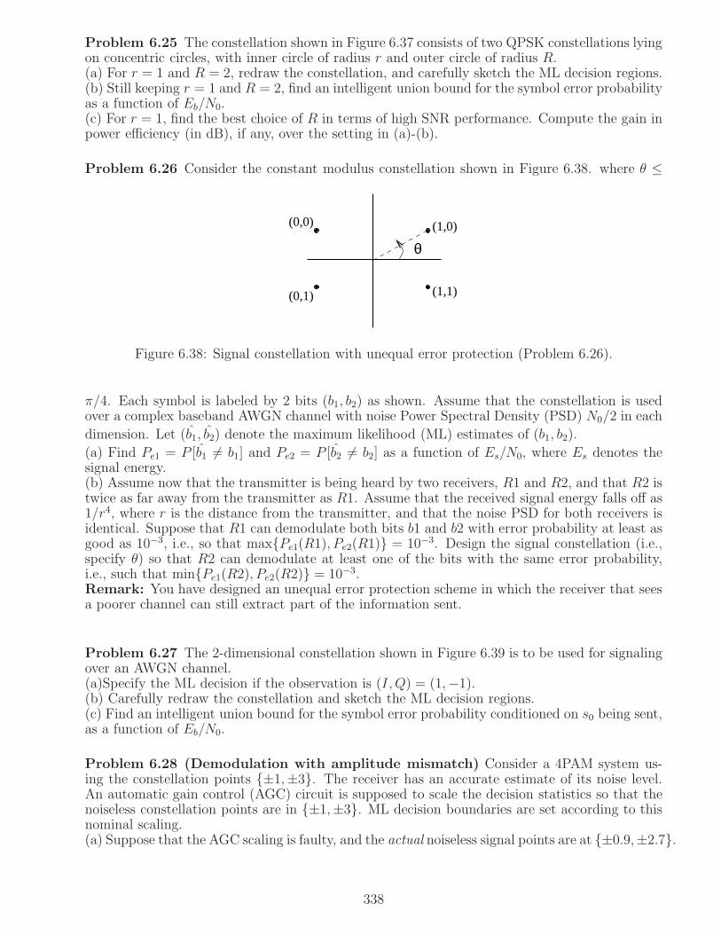
Problem 6.25 The constellation shown in Figure 6.37 consists of two QPSK constellations lyingon concentric circles, with inner circle of radius r and outer circle of radius R.(a) For r = 1 and R = 2, redraw the constellation, and carefully sketch the ML decision regions.(b) Still keeping r = 1 and R = 2, find an intelligent union bound for the symbol error probabilityas a function of Eb/N0.(c) For r = 1, find the best choice of R in terms of high SNR performance. Compute the gain inpower efficiency (in dB), if any, over the setting in (a)-(b).

Problem 6.26 Consider the constant modulus constellation shown in Figure 6.38. where θ ≤

(0,1)

(0,0) (1,0)

(1,1)

θ

Figure 6.38: Signal constellation with unequal error protection (Problem 6.26).

π/4. Each symbol is labeled by 2 bits (b1, b2) as shown. Assume that the constellation is usedover a complex baseband AWGN channel with noise Power Spectral Density (PSD) N0/2 in each

dimension. Let (b1, b2) denote the maximum likelihood (ML) estimates of (b1, b2).

(a) Find Pe1 = P [b1 6= b1] and Pe2 = P [b2 6= b2] as a function of Es/N0, where Es denotes thesignal energy.(b) Assume now that the transmitter is being heard by two receivers, R1 and R2, and that R2 istwice as far away from the transmitter as R1. Assume that the received signal energy falls off as1/r4, where r is the distance from the transmitter, and that the noise PSD for both receivers isidentical. Suppose that R1 can demodulate both bits b1 and b2 with error probability at least asgood as 10−3, i.e., so that maxPe1(R1), Pe2(R1) = 10−3. Design the signal constellation (i.e.,specify θ) so that R2 can demodulate at least one of the bits with the same error probability,i.e., such that minPe1(R2), Pe2(R2) = 10−3.Remark: You have designed an unequal error protection scheme in which the receiver that seesa poorer channel can still extract part of the information sent.

Problem 6.27 The 2-dimensional constellation shown in Figure 6.39 is to be used for signalingover an AWGN channel.(a)Specify the ML decision if the observation is (I, Q) = (1,−1).(b) Carefully redraw the constellation and sketch the ML decision regions.(c) Find an intelligent union bound for the symbol error probability conditioned on s0 being sent,as a function of Eb/N0.

Problem 6.28 (Demodulation with amplitude mismatch) Consider a 4PAM system us-ing the constellation points ±1,±3. The receiver has an accurate estimate of its noise level.An automatic gain control (AGC) circuit is supposed to scale the decision statistics so that thenoiseless constellation points are in ±1,±3. ML decision boundaries are set according to thisnominal scaling.(a) Suppose that the AGC scaling is faulty, and the actual noiseless signal points are at ±0.9,±2.7.

338

0

0s3

s1

s2

31

2

−2

−3I

Q

−1

s


Sketch the points and the mismatched decision regions. Find an intelligent union bound for thesymbol error probability in terms of the Q function and Eb/N0.(b) Repeat (a), assuming that faulty AGC scaling puts the noiseless signal points at ±1.1,±3.3.(c) AGC circuits try to maintain a constant output power as the input power varies, and can beviewed as imposing a scale factor on the input inversely proportional to the square root of theinput power. In (a), does the AGC circuit overestimate or underestimate the input power?

Problem 6.29 (Demodulation with phase mismatch) Consider a BPSK system in whichthe receiver’s estimate of the carrier phase is off by θ.(a) Sketch the I and Q components of the decision statistic, showing the noiseless signal pointsand the decision region.(b) Derive the BER as a function of θ and Eb/N0 (assume that θ < π

2).

(c) Assuming now that θ is a random variable taking values uniformly in [−π4, π4], numerically

compute the BER averaged over θ, and plot it as a function of Eb/N0. Plot the BER withoutphase mismatch as well, and estimate the dB degradation due to the phase mismatch.

Problem 6.30 (Simplex signaling set) Let s0(t), ..., sM−1(t) denote a set of equal energy,orthogonal signals. Construct a new M-ary signal set from these as follows, by subtracting outthe average of the M signals from each signal as follows:

uk(t) = sk(t)−1

M

M−1∑

j=0

sj(t) , k = 0, 1, ..,M − 1

This is called the simplex signaling set.(a) Find a union bound on the symbol error probability, as a function of Eb/N0 and M , forsignaling over the AWGN channel using the signal set uk(t), k = 0, 1, ...,M − 1.(b) Compare the power efficiencies of the simplex and orthogonal signaling sets for a given M ,and use these to estimate the performance difference in dB between these two signaling schemes,for M = 4, 8, 16, 32. What happens as M gets large?(c) Use computer simulations to plot, for M = 4, the error probability (log scale) versus Eb/N0

(dB) of the simplex signaling set and the corresponding orthogonal signaling set. Are your resultsconsistent with the prediction from (b)?

Problem 6.31 (Soft decisions for BPSK) Consider a BPSK system in which 0 and 1 areequally likely to be sent, with 0 mapped to +1 and 1 to -1 as usual. Thus, the decision statisticY = A +N if 0 is sent, and Y = −A+N if 1 is sent, where A > 0 and N ∼ N(0, σ2).

339

(a) Show that the LLR is conditionally Gaussian given the transmitted bit, and that the condi-tional distribution is scale-invariant, depending only on Eb/N0.(b) If the BER for hard decisions is 10%, specify the conditional distribution of the LLR, giventhat 0 is sent.

Problem 6.32 (Soft decisions for PAM) Consider soft decisions for 4PAM signaling as inExample 6.1.3. Assume that the signals have been scaled to ±1,±3 (i.e., set A = 1 in Example6.1.3. The system is operating at Eb/N0 of 6 dB. Bits b1, b2 ∈0, 1 are mapped to the symbolsusing Gray coding. Assume that (b1, b2) = (0, 0) for symbol -3, and (1, 0) for symbol +3.(a) Sketch the constellation, along with the bit maps. Indicate the ML hard decision boundaries.(b) Find the posterior symbol probability P [−3|y] as a function of the noisy observation y. Plotit as a function of y.Hint: The noise variance σ2 can be inferred from the signal levels and SNR.(c) Find P [b1 = 1|y] and P [b2 = 1|y], and plot as a function of y.Remark: The posterior probability of b1 = 1 equals the sum of the posterior probabilities of allsymbols which have b1 = 1 in their labels.(d) Display the results of part (c) in terms of LLRs.

LLR1(y) = logP [b1 = 0|y]P [b1 = 1|y] , LLR2(y) = log

P [b2 = 0|y]P [b2 = 1|y]

Plot the LLRs as a function of y, saturating the values as ±50.(e) Try other values of Eb/N0 (e.g., 0 dB, 10 dB). Comment on any trends you notice. How dothe LLRs vary as a function of distance from the noiseless signal points? How do they vary asyou change Eb/N0.(f) In order to characterize the conditional distribution of the LLRs, simulate the system overmultiple symbols at Eb/N0 such that the BER is about 5%. Plot the histograms of the LLRsfor each of the two bits, and comment on whether they look Gaussian. What happens as youincrease or decrease Eb/N0?

Problem 6.33 (M-ary orthogonal signaling performance as M → ∞) We wish to derivethe result that

limM→∞

P (correct) =

1 Eb

N0> ln 2

0 Eb

N0< ln 2

(6.92)

(a) Show that

P (correct) =

∫ ∞

−∞

[

Φ

(

x+

√

2Eb log2M

N0

)]M−11√2πe−x2/2 dx

(b) Show that, for any x,

limM→∞

[

Φ

(

x+

√

2Eb log2M

N0

)]M−1

=

0 Eb

N0< ln 2

1 Eb

N0> ln 2

Hint: Use L’Hospital’s rule on the log of the expression whose limit is to be evaluated.(c) Substitute (b) into the integral in (a) to infer the desired result.

Problem 6.34 (Effect of Rayleigh fading) Constructive and destructive interference betweenmultiple paths in wireless systems lead to large fluctuations in received amplitude, modeled as a

340

Rayleigh random variable A (see Problem 5.21 for a definition). The energy per bit is thereforeproportional to A2, which, using Problem 5.21(c), is an exponential random variable. Thus,we can model Eb/N0 as an exponential random variable with mean Eb/N0, where Eb is theaverage energy per bit. Simplify notation by setting Eb

N0= X , and the mean Eb/N0 =

1µ, so that

X ∼ Exp(µ).(a) Show that the average error probability for BPSK with Rayleigh fading can be written as

Pe =

∫ ∞

0

Q(√2x) µe−µx dx

Hint: The error probability for BPSK is given by Q(√

2Eb

N0

)

, where Eb/N0 is a random variable.

We now find the expected error probability by averaging over the distribution of Eb/N0.(b) Integrating by parts and simplifying, show that the average error probability can be writtenas

Pe =1

2

(

1− (1 + µ)−12

)

=1

2

(

1− (1 +N0

Eb

)−12

)

Hint: Q(x) is defined via an integral, so we can find its derivative (when integrating by parts)using the fundamental theorem of calculus.(c) Using the approximation that (1 + a)b ≈ 1 + ba for |a| small, show that

Pe ≈1

4(Eb/N0)

at high SNR. Comment on how this decay of error probability with the reciprocal of SNRcompares with the decay for the AWGN channel.

(b) Plot the error probability versus Eb

N0for BPSK over the AWGN and Rayleigh fading channels

(BER on log scale, EN0

in dB). Note that Eb = Eb for the AWGN channel. At BER of 10−3, whatis the degradation in dB due to Rayleigh fading?

Link budget analysis

Problem 6.35 You are given an AWGN channel of bandwidth 3 MHz. Assume that implemen-tation constraints dictate an excess bandwidth of 50%. Find the achievable bit rate, the Eb/N0

required for a BER of 10−8, and the receiver sensitivity (assuming a receiver noise figure of 7dB) for the following modulation schemes, assuming that the bit-to-symbol map is optimized tominimize the BER whenever possible:(a) QPSK, (b) 8PSK, (c) 64QAM (d) Coherent 16-ary orthogonal signaling.Remark: Use nearest neighbors approximations for the BER.

Problem 6.36 Consider the setting of Example 6.5.1.(a) For all parameters remaining the same, find the range and bit rate when using a 64QAMconstellation.(b) Suppose now that the channel model is changed from AWGN to Rayleigh fading (see Problem6.34). Find the receiver sensitivity required for QPSK at BER of 10−5. (In practice, we wouldshoot for a higher uncoded BER, and apply channel coding, but we discuss such methods in laterchapters.) What is the range, assuming all other parameters are as in Example 6.5.1? How doesthe range change if you reduce the link margin to 10 dB (now that fading is being accounted for,there are fewer remaining uncertainties).

341

Problem 6.37 Consider a line-of-sight communication link operating in the 60 GHz band (wherelarge amounts of unlicensed bandwidth have been set aside by regulators). From version 1 ofthe Friis formula (6.83), we see that the received power scales as λ2, and hence as the inversesquare of the carrier frequency, so that 60 GHz links have much worse propagation than, say, 5GHz links when antenna gains are fixed. However, from (6.82), we see that the we can get muchbetter antenna gains at small carrier wavelengths for a fixed form factor, and version 2 of theFriis formula (6.84) shows that the received power scales as 1/λ2, which improves with increasingcarrier frequency. Furthermore, electronically steerable antenna arrays with high gains can beimplemented with compact form factor (e.g., patterns of metal on circuit board) at higher carrierfrequencies such as 60 GHz. Suppose, now, that we wish to design a 2 Gbps link using QPSKwith an excess bandwidth of 50%. The receiver noise figure is 8 dB, and the desired link marginis 10 dB.(a) What is the transmit power in dBm required to attain a range of 10 meters (e.g., for in-roomcommunication), assuming that the transmit and receive antenna gains are each 10 dBi?(b) For a transmit power of 20 dBm, what are the antenna gains required at the transmitter andreceiver (assume that the gains at both ends are equal) to attain a range of 200 meters (e.g., foran outdoor last-hop link)?(c) For the antenna gains found in (b), what happens to the attainable range if you account foradditional path loss due to oxygen absorption (typical in the 60 GHz band) of 16 dB/km?(d) In (c), what happens to the attainable range if there is a further path loss of 30 dB/km dueto heavy rain (on top of the loss due to oxygen absorption)?

Problem 6.38 A 10 Mbps line-of-sight communication link operating at a carrier frequency of1 GHz has a designed range of 5 km. The link employs 16QAM with an excess bandwidth of25%, with a designed BER of 10−6 and a link margin of 10 dB. The receiver noise figure is 4dB, and the transmit and receive antenna gains are 10 dBi each. This is the baseline scenarioagainst which each of the scenarios in (a)-(c) are to be compared.(a) Suppose that you change the carrier frequency to 5 GHz, keeping all other link parametersthe same. What is the new range?(b) Suppose that you change the carrier frequency to 5 GHz and increase the transmit and receiveantenna gains by 3 dBi each, keeping all other link parameters the same. What is the new range?(c) Suppose you change the carrier frequency to 5 GHz, increase the transmit and receive antennadirectivities by 3 dBi each, and increase the data rate to 40 Mbps, still using 16QAM with excessbandwidth of 25%. All other link parameters are the same. What is the new range?

Software Lab 6.1: Linear modulation with two-dimensional

constellations

This is a follow-on to Software Lab 4.1, the code from which is our starting point here. Theobjective is to implement in complex baseband a linearly modulated system for a variety of signalconstellations. We wish to estimate the performance of these schemes for an ideal channel viasimulation, and to compare with analytical expressions. As in Software Lab 4.1, we use atrivial channel filter in this lab. Dispersive channels are considered in Chapter 7 and theassociated labs.

0) Use the code for Software Lab 4.1 as a starting point.

1) Write a matlab function randbit that generates random bits taking values in 0, 1 (not ±1)with equal probability.

2) Write the following functions mapping bits to symbols for different signal constellations. Writethe functions to allow for vector inputs and outputs. The mapping is said to be a Gray

342

code, or Gray labeling, if the bit map for nearest neighbors in the constellation differ by exactlyone bit. In all of the following, choose the bit map to be a Gray code.(a) bpskmap: input a 0/1 bit, output a ±1 bit.(b) qpskmap: input 2 0/1 bits, output a symbol taking one of four values in ±1± j.(c) fourpammap: input 2 0/1 bits, output a symbol taking one of four values in ±1,±3.(d) sixteenqammap: input 4 0/1 bits, output a symbol taking one of 16 values in bc + jbs :bc, bs ∈±1,±3.(e) eightpskmap: input 3 0/1 bits, output a symbol taking one of 8 values in ej2πi/8, i = 0, 1, ..., 7.

3) BPSK symbol generation: Use part 1 to generate 12000 0/1 bits. Map these to BPSK (±1)bits using bpskmap. Pass these through the transmit and receive filter in lab 1 to get noiselessreceived samples at rate 4/T , as before.

4) Adding noise: We consider discrete time additive white Gaussian noise (AWGN). At the inputto the receive filter, add independent and identically distributed (iid) complex Gaussian noise,such that the real and imaginary part of each sample are iid N(0, σ2) (you will choose σ2 = N0

2

corresponding to a specified value of Eb

N0, as described in part 5. Pass these (rate 4/T ) noise

samples through the receive filter, and add the result to the output of part 3.

Remark: If the nth transmitted symbol is b[n], the average received energy per symbol isEs = E[|b[n]|2]||gT ∗ gC ||2. Divide that by the number of bits per symbol to get Eb. Thenoise variance per dimension is σ2 = N0

2. This enables you to compute Eb/N0 for your simula-

tion model. The signal-to-noise ratio Eb/N0 is usually expressed in decibels (dB): Eb/N0(dB) =10 log10Eb/N0(raw). Thus, if you fix the transmit and channel filter coefficients, then you cansimulate any given value of Eb/N0 in dB by varying the value of the noise variance σ2.

5) Plot the ideal bit error probability for BPSK, which is given by Q(√

2Eb/N0), on a log scaleas a function of Eb/N0 in dB over the range 0-10 dB. Find the value of Eb/N0 that correspondsto an error probability of 10−2.

6) For the value of Eb/N0 found in part 5, choose the corresponding value of σ2 in part 1. Findthe decision statistics corresponding to the transmitted symbols at the input and output of thereceive filter, as in lab 1 (parts 5 and 6). Plot the imaginary versus the real parts of the decisionstatistics; you should see a noisy version of the constellation.

7) Using an appropriate decision rule, make decisions on the 12000 transmitted bits based onthe 12000 decision statistics, and measure the error probability obtained at the input and theoutput. Compare the results with the ideal error probability from part 5. You should find thatthe error probability based on the receiver input samples is significantly worse than that basedon the receiver output, and that the latter is a little worse than the ideal performance becauseof the ISI in the decision statistics.

8) Now, map 12000 0/1 bits into 6000 4PAM symbols using function fourpammap (use as input2 parallel vectors of 6000 bits). As shown in Chapter 6, a good approximation (the nearestneighbors approximation) to the ideal bit error probability for Gray coded 4PAM is given by

Q(√

4Eb

5N0

)

. As in part 5), plot this on a log scale as a function of Eb/N0 in dB over the range

0-10 dB. What is the value of Eb/N0 (dB) corresponding to a bit error probability of 10−2?

9) Choose the value of the noise variance σ2 corresponding to the Eb/N0 found in part 7. Now,find decision statistics for the 6000 transmitted symbols based on the receive filter output only.(a) Plot the imaginary versus the real parts of the decision statistics, as before.(b) Determine an appropriate decision rule for estimating the two parallel bit streams of 6000bits from the 6000 complex decision statistics.(c) Measure the bit error probability, and compare it with the ideal bit error probability.

10) Repeat parts 8 and 9 for QPSK, the ideal bit error probability for which, as a function of

343

Eb/N0, is the same as for BPSK.

11) Repeat parts 8 and 9 for 16QAM (4 bit streams of length 3000 each), the ideal bit errorprobability for which, as a function of Eb/N0, is the same as for 4PAM.

12) Repeat parts 8 and 9 for 8PSK (3 bit streams of length 4000 each). The ideal bit errorprobability for Gray coded 8PSK is approximated by (using the nearest neighbors approximation)

Q

(

√

(6−3√2)Eb

2N0

)

.

13) Since all your answers above will be off from the ideal answers because of some ISI, run asimulation with 12000 bits sent using Gray-coded 16-QAM with no ISI. To do this, generate thedecision statistics by adding noise directly to the transmitted symbols, setting the noise varianceappropriately to operate at the required Eb/N0. Do this for two different values of Eb/N0, the onein part 11 and a value 3 dB higher. In each case, compare the nearest neighbors approximationto the measured bit error probability, and plot the imaginary versus real part of the decisionstatistics.

Lab Report: Your lab report should document the results of the preceding steps in order. Describethe reasoning you used and the difficulties you encountered.

Tips: Vectorize as many of the functions as possible, including both the bit-to-symbol maps andthe decision rules. Do BPSK and 4-PAM first, where you will only use the real part of the complexdecision statistics. Leverage this for QPSK and 16-QAM, by replicating what you did for theimaginary part of the decision statistics as well. To avoid confusion, keep different matlab filesfor simulations regarding different signal constellations, and keep the analytical computationsand plots separate from the simulations.

Software Lab 6.2: Modeling and performance evaluation

on a wireless fading channel

Let us consider the following simple model of a wireless channel (obtained after filtering andsampling at the symbol rate, and assuming that there is no ISI). If b[n] is the transmittedsymbol sequence, then the complex-valued received sequence is given by

y[n] = h[n]b[n] + w[n] (6.93)

where w[n] = wc[n] + jws[n] is an iid complex Gaussian noise sequence with wc[n], ws[n] i.i.d.N(0, σ2 = N0

2) random variables. We say that w[n] has variance σ2 per dimension. The channel

sequence h[n] is a time-varying sequence of complex gains.

Equation (6.93) models the channel at a given time as a simple scalar gain h[n]. On the otherhand, as discussed in Example 2.5.4, a multipath wireless channel cannot be modeled as a simplescalar gain: it is dispersive in time, and exhibits frequency selectivity. However, it is shown inChapter 8 that we can decompose complicated dispersive channels into scalar models by usingfrequency-domain modulation, or OFDM, which transmits data in parallel over narrow enoughfrequency slices such that the channel over each slice can be modeled as a complex scalar.Equation (6.93) could therefore be interpreted as modeling time variations in such scalar gains.

Rayleigh fading: The channel gain sequence h[n] = hc[n]+jhs[n], where hc[n] and hs[n]are zero mean, independent and identically distributed colored Gaussian random processes. Thereason this is called Rayleigh fading is that |h[n]| =

√

h2c [n] + h2s[n] is a Rayleigh random variable.Remark: The Gaussianity arises because the overall channel gain results from a superposition ofgains from multiple reflections off scatterers.

344

Simulation of Rayleigh fading: We will use a simple model wherein the colored channel gainsequence h[n] is obtained by passing white Gaussian noise through a first-order recursive filter,as follows:

hc[n] = ρhc[n− 1] + u[n]hs[n] = ρhs[n− 1] + v[n]

(6.94)

where u[n] and v[n] are independent real-valued white Gaussian sequences, with i.i.d. N(0, β2)elements. The parameter ρ (0 < ρ < 1) determines how rapidly the channel varies. The model forI and Q gains in (6.94) are examples of first-order autoregressive (AR(1)) random processes: au-toregressive because future values depend on the past in a linear fashion, and first order becauseonly the immediately preceding value affects the current one.

Setting up the fading simulator

(a) Set up the AR(1) Rayleigh fading model in matlab, with ρ and β2 as programmable param-eters.

(b) Calculate E[|h[n]|2] = 2E [h2c [n]] = 2v2 analytically as a function of ρ and β2. Use simulationto verify your results, setting ρ = .99 and β = .01. You may choose to initialize hc[0] and hs[0]as iid N(0, v2) in your simulation. Use at least 10,000 samples.

(c) Plot the instantaneous channel power relative to the average channel power, |h[n]|22v2

in dB asa function of n. Thus, 0 dB corresponds to the average value of 2v2. You will occasionally seesharp dips in the power, which are termed deep fades.

(d) Define the channel phase θ[n] = angle(h[n]) = tan−1 hs[n]hc[n]

. Plot θ[n] versus n. Compare with

(c); you should see sharp phase changes corresponding to deep fades.

QPSK in Rayleigh fading

Now, implement the model (6.93), where b[n] correspond to Gray coded QPSK, using an AR(1)simulation of Rayleigh fading as in (a). Assume that the receiver has perfect knowledge of thechannel gains h[n], and employs the decision statistic Z[n] = h∗[n]y[n].Remark: In practice, the channel estimation required for implementing this is achieved by insert-ing pilot symbols periodically into the data stream. The performance will, of course, be worsethan with the ideal channel estimates considered here.

(e) Do scatter plots of the two-dimensional received symbols y[n], and of the decision statisticsZ[n]. What does multiplying by h∗[n] achieve?

(f) Implement a decision rule for the bits encoded in the QPSK symbols based on the statisticsZ[n]. Estimate by simulation, and plot, the bit error probability (log scale) as a function ofthe average Eb/N0 (dB), where Eb/N0 ranges from 0 to 30 dB. Use at least 10,000 symbols foryour estimate. On the same plot, also plot the analytical bit error probability as a function ofEb/N0 when there is no fading. You should see a marked degradation due to fading. How doyou think the error probability in fading varies with Eb/N0?

Relating simulation parameters to Eb/N0: The average symbol energy is Es = E[|b[n]|2]E[|h[n]|2],and Eb =

Es

log2 M. This is a function of the constellation scaling and the parameters β2 and ρ in

the fading simulator (see (b)). You can therefore fix Es, and hence Eb, by fixing β, ρ (e.g., as in(b)), and fix the scaling of the b[n] (e.g., keep the constellation points as ±1± j). Eb/N0 cannow be varied by varying the variance σ2 of the noise in (6.93).

Diversity

The severe degradation due to Rayleigh fading can be mitigated by using diversity: the proba-bility that two paths are simultaneously in a deep fade is less likely than the probability that asingle path is in a deep fade. Consider a receive antenna diversity system, where the received

345

signals y1 and y2 at the two antennas are given by

y1[n] = h1[n]b[n] + w1[n]y2[n] = h2[n]b[n] + w2[n]

(6.95)

Thus, you get two looks at the data stream, through two different channels.

Implement the two-fold diversity system in (6.95) as you implemented (6.93), keeping the fol-lowing in mind:• The noises w1 and w2 are independent white noise sequences with variance σ2 = N0

2per di-

mension as before.• The channels h1 and h2 are generated by passing independent white noise streams through afirst-order recursive filter. In relating the simulation parameters to Eb/N0, keep in mind that theaverage symbol energy now is Es = E[|b[n]|2]E[|h1[n]|2 + |h2[n]|2].• Use the following maximal ratio combining rule to obtain the decision statistic

Z2[n] = h∗1[n]y1[n] + h∗2[n]y2[n]

The decision statistic above can be written as

Z2[n] = (|h1[n]|2 + |h2[n]|2)b[n] + w[n]

where w[n] is zero mean complex Gaussian with variance σ2(|h1[n]|2 + |h2[n]|2) per dimension.Thus, the instantaneous SNR is given by

SNR[n] =E

[

|(|h1[n]|2 + |h2[n]|2)b[n]|2]

E [|w[n]|2] =|h1[n]|2 + |h2[n]|2E[|b[n]|2]

2σ2

(g) Plot |h1[n]|2 + |h2[n]|2 in dB as a function of n, with 0 dB representing the average value asbefore. You should find that the fluctuations around the average are less than in (c).

(h) Implement a decision rule for the bits encoded in the QPSK symbols based on the statisticsZ2[n]. Estimate by simulation, and plot (on the same plot as in (e)), the bit error probability(log scale) as a function of the average Eb/N0 (dB), where Eb/N0 ranges from 0 to 30 dB. Useat least 10,000 symbols for your estimate. You should see an improvement compared to thesituation with no diversity.

Lab Report: Your lab report should document the results of the preceding steps in order.Describe the reasoning you used and the difficulties you encountered.

Bonus: A Glimpse of differential modulation and demodulation

Throughout this chapter, we have assumed that a noiseless “template”” for the set of possibletransmitted signals is available at the receiver. In the present context, it means assuming thatestimates for the time-varying fading channel are available. But what is these estimates, whichwe used to generate the decision statistics earlier in this lab, are not available? One approach thatavoids the need for explicit channel estimation is based on exploiting the fact that the channeldoes not change much from symbol to symbol. Let us illustrate this for the case of QPSK. Themodel is exactly as in (6.93) or (6.95), but the channel sequence(s) is(are) unknown a priori. Thisnecessitates encoding the data in a different way. Specifically, let d[n] be a Gray coded QPSKinformation sequence, which contains information about the bits of interest. Instead of sendingd[n] directly, we generate the transmitted sequence b[n] by differential encoding as follows:

b[n] = d[n]b[n− 1], n = 1, 2, 3, 4, ..

346

(You can initialize b(0) as any element of the constellation, known by agreement to both trans-mitter and receiver. Or, just ignore the first information symbol in your demodulation). Atthe receiver, use differential demodulation to generate the decision statistic for the informationsymbol d[n] as follows:

Znc[n] = y[n]y∗[n− 1] single path

Znc2 [n] = y1[n]y

∗1[n− 1] + y2[n]y

∗2[n− 1] dual diversity

where the superscript indicates noncoherent demodulation, i.e., demodulation that does notrequire an explicit channel estimate.

Bonus assignment report: Estimate by simulation, and plot, the bit error probability of Graycoded differentially encoded QPSK as a function of Eb/N0 for both single path and dual diversity.Compare with the curves for coherent demodulation that you have obtained earlier. How much(in dB) does the performance degrade by? Document your results as in the earlier lab reports.

6.A Irrelevance of component orthogonal to signal space

Conditioning on Hi, we have y(t) = si(t)+n(t). The component of the received signal orthogonalto the signal space is given by

y⊥(t) = y(t)− yS(t) = y(t)−n−1∑

k=0

Y [k]ψk(t) = si(t) + n(t)−n−1∑

k=0

(si[k] +N [k])ψk(t)

But the signal si(t) lies in the signal space, so that

si(t)−n−1∑

k=0

si[k]ψk(t) = 0

That is, the signal contribution to y⊥ is zero, and

y⊥(t) = n(t)−n−1∑

k=0

N [k]ψk(t) = n⊥(t)

where n⊥ denotes the noise projection orthogonal to the signal space.

We now show that n⊥(t) is independent of the signal space noise vector N. Since n⊥ and N arejointly Gaussian, it suffices to show that they are uncorrelated. For any t and k, we have

cov(n⊥(t), N [k]) = E[n⊥(t)N [k]] = E

[

n(t)−∑n−1j=0 N [j]ψj(t)N [k]

]

= E[n(t)N [k]]−∑n−1j=0 E[N [j]N [k]]ψj(t)

(6.96)

The first term on the extreme right-hand side can be simplified as

E[n(t)〈n, ψk〉] = E[n(t)

∫

n(s)ψk(s)ds] =

∫

E[n(t)n(s)]ψk(s)ds =

∫

σ2δ(s−t)ψk(s)ds = σ2ψk(t)

(6.97)Plugging (6.97) into (6.96), and noting that E[N [j]N [k]] = σ2δjk, we obtain that

cov(n⊥(t), N [j]) = σ2ψk(t)− σ2ψk(t) = 0

347

What we have just shown is that the component of the received signal orthogonal to the signalspace contains the noise component n⊥ only, and thus does not depend on which signal is sentunder a given hypothesis. Since n⊥ is independent of N, the noise vector in the signal space,knowing n⊥ does not provide any information about N. These two observations imply that y⊥

is irrelevant for our hypothesis problem. The preceding discussion is illustrated in Figure 6.9,and enables us to reduce our infinite-dimensional problem to a finite-dimensional vector modelrestricted to the signal space.

Note that our irrelevance argument depends crucially on the property of WGN that its projec-tions along orthogonal directions are independent. Even though y⊥ does not contain any signalcomponent (since these by definition fall into the signal space), if n⊥ and N exhibited statis-tical dependence, one could hope to learn something about N from n⊥, and thereby improveperformance compared to a system in which y⊥ is thrown away. However, since n⊥ and N areindependent for WGN, we can restrict attention to the signal space for our hypothesis testingproblem.

348

Chapter 7

Channel Coding

We have seen in Chapter 6 that, for signaling over an AWGN channel, the error probabilitydecays exponentially with SNR, with the rate of decay determined by the power efficiency ofthe constellation. For example, for BPSK or Gray coded QPSK, the error probability is given

by p = Q(√

2Eb

N0

)

. We have also seen in Chapter 6 how to engineer the link budget so as

to guarantee a certain desired performance. So far, however, we have only considered uncodedsystems, in which bits to be sent are directly mapped to symbols sent over the channel. Wenow indicate how it is possible to improve performance by channel coding, which corresponds toinserting redundancy strategically prior to transmission over the channel.

A bit of historical perspective is in order. As mentioned in Chapter 1, Shannon showed theoptimality of separate source and channel coding back in 1948. Shannon also provided a theoryfor computing the limits of communication performance over any channel (given constraintssuch as power and bandwidth). He did not provide a constructive means of attaining theselimits; his proofs employed randomized constructions. For reasons of computational complexity,it was assumed that such strategies could never be practical. Hence, for decades after Shannon’s1948 publication, researchers focused on algebraic constructions (for which decoding algorithmsof reasonable complexity could be devised) to create powerful channel codes, but never quitesucceeded in attaining Shannon’s benchmarks. This changed with the invention of turbo codesby Berrou et al in 1993: their conference paper laid out a simple coding strategy that got to withina dB of Shannon capacity. They took codes which were easy to encode, and used scramblers tomake them random-like. Maximum likelihood decoding for such codes is too computationallycomplex, but Berrou et al showed that suboptimal iterative decoding methods provide excellentperformance with reasonable complexity. It was then realized that a different class of random-like codes, called low density parity check (LDPC) codes, along with an appropriate iterativedecoding procedure, had actually been invented by Gallager in the 1960s. Since then, there hasbeen a massive effort to devise and implement a wide variety of “turbo-like” codes (i.e., random-like codes amenable to iterative decoding), with the result that we can now approach Shannon’sperformance benchmarks over almost any channel.

In this chapter, we provide a glimpse of how Shannon’s performance benchmarks are computed,how channel codes are constructed, and how iterative decoding works. A systematic and com-prehensive treatment of information theory and channel coding would take up entire textbooksin itself, hence our goal is to provide just enough exposure to some of the key ideas to encouragefurther exploration.

Chapter Plan: In Section 7.1, we discuss two extreme examples, uncoded transmission andrepetition coding, in order to motivate the need for more sophisticated channel coding strategies.A generic model for channel coding is discussed in Section 7.2. Section 7.3 introduces Shannon’sinformation-theoretic framework, which provides fundamental performance limits for any chan-

349

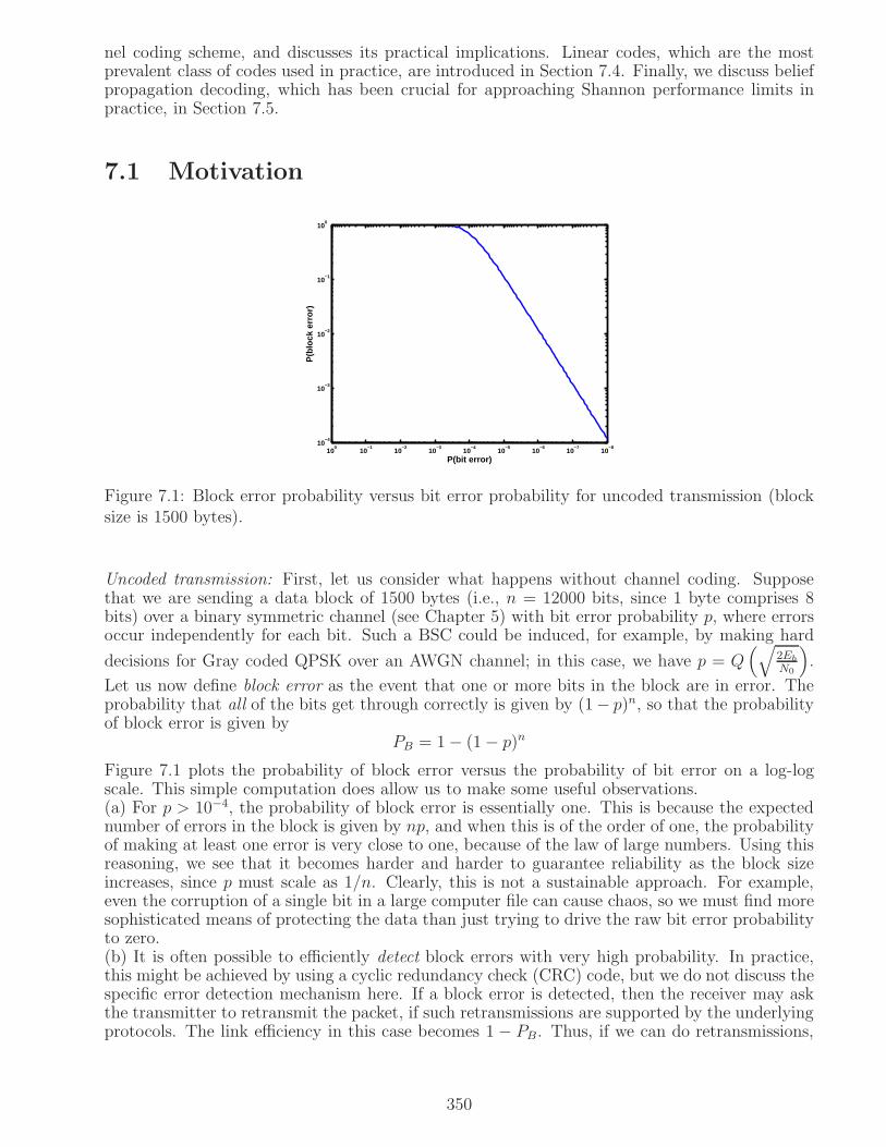
nel coding scheme, and discusses its practical implications. Linear codes, which are the mostprevalent class of codes used in practice, are introduced in Section 7.4. Finally, we discuss beliefpropagation decoding, which has been crucial for approaching Shannon performance limits inpractice, in Section 7.5.

7.1 Motivation

10−8

10−7

10−6

10−5

10−4

10−3

10−2

10−1

100

10−4

10−3

10−2

10−1

100

P(bit error)

P(b

lock

err

or)

Figure 7.1: Block error probability versus bit error probability for uncoded transmission (blocksize is 1500 bytes).

Uncoded transmission: First, let us consider what happens without channel coding. Supposethat we are sending a data block of 1500 bytes (i.e., n = 12000 bits, since 1 byte comprises 8bits) over a binary symmetric channel (see Chapter 5) with bit error probability p, where errorsoccur independently for each bit. Such a BSC could be induced, for example, by making hard

decisions for Gray coded QPSK over an AWGN channel; in this case, we have p = Q(√

2Eb

N0

)

.

Let us now define block error as the event that one or more bits in the block are in error. Theprobability that all of the bits get through correctly is given by (1− p)n, so that the probabilityof block error is given by

PB = 1− (1− p)n

Figure 7.1 plots the probability of block error versus the probability of bit error on a log-logscale. This simple computation does allow us to make some useful observations.(a) For p > 10−4, the probability of block error is essentially one. This is because the expectednumber of errors in the block is given by np, and when this is of the order of one, the probabilityof making at least one error is very close to one, because of the law of large numbers. Using thisreasoning, we see that it becomes harder and harder to guarantee reliability as the block sizeincreases, since p must scale as 1/n. Clearly, this is not a sustainable approach. For example,even the corruption of a single bit in a large computer file can cause chaos, so we must find moresophisticated means of protecting the data than just trying to drive the raw bit error probabilityto zero.(b) It is often possible to efficiently detect block errors with very high probability. In practice,this might be achieved by using a cyclic redundancy check (CRC) code, but we do not discuss thespecific error detection mechanism here. If a block error is detected, then the receiver may askthe transmitter to retransmit the packet, if such retransmissions are supported by the underlyingprotocols. The link efficiency in this case becomes 1 − PB. Thus, if we can do retransmissions,

350

uncoded transmission may actually not be a terrible idea. In our example, the link is 90% efficient(PB = 10−1) for bit error probability p around 10−6 − 10−5, and 99% efficient (PB = 10−2) for paround 10−7 − 10−6.

(c) For Gray coded QPSK, p = Q(√

2Eb

N0

)

, so that p = 10−6 requires Eb/N0 of about 10.55 dB.

This is exactly the scenario in the link budget example modeling a 5 GHz WLAN link in Chapter6. We see, therefore, that uncoded transmission, along with retransmissions, is a viable optionin that setting.

2 4 6 8 10 12 14 16 18 20 2210

−20

10−18

10−16

10−14

10−12

10−10

10−8

10−6

10−4

10−2

n

P(b

lock

err

or)

p=0.1p=0.01

Figure 7.2: Error probability decays rapidly as a function of blocklength for a repetition code.

Repetition coding: Next, let us consider the other extreme, in which we send n copies of a singlebit over a BSC with error probability p. That is, we either send a string of n zeros, or a string ofn ones. The channel may flip some of these bits; since the errors are independent, the number oferrors is a binomial random variable, Bin(n, p). For p < 1

2, the average number of bits in error,

np < n/2, hence a natural decoding rule is to employ majority logic: decide on 0 if the majorityof received bits is zero, and on 1 otherwise. Taking n to be odd for simplicity (otherwise weneed to specify a tiebreaker when there are an equal number of zeros and ones), a block erroroccurs if the number of errors is ⌈n/2⌉ or more. Using the binomial PMF, we have the followingexpression for the block error probability:

PB =

n∑

m=⌈n/2⌉

(

nm

)

pm(1− p)m

Figure 7.2 plots the probability of block error versus n for p = 10−1 and p = 10−2. Clearly,PB → 0 as n→ ∞, so we are doing well in terms of reliability. To see why, let us invoke the LLNagain: the average number of errors is np < ⌈n/2⌉, so that, as n → ∞, the number of errors issmaller than ⌈n/2⌉ with probability one. However, we are only sending one bit of information forevery n bits that we send over the channel, corresponding to a code rate of 1/n (one informationbit for every n transmitted bits), which tends to zero as n→ ∞.

We have invoked the LLN to explain the performance of both uncoded transmission and repetitioncoding for large n, but neither of these approaches provides reliable performance at nonzerocoding rates. As n → ∞, the block error rate PB → 1 for uncoded transmission, while thecode rate tends to zero for the repetition code. However, it is possible to design channel codingschemes between these two extremes which provide arbitrarily reliable communication (PB → 0as n→ ∞) at non-vanishing code rates. The existence of such codes is guaranteed by LLN-stylearguments. For example, for a BSC with crossover probability p, as n gets large, the number

351

of errors clusters around np. Thus, the basic intuition is that, if we are able to insert enoughredundancy to correct a number of errors of the order of np, then we should be able to approachzero block error probability. Giving precise form to such existence arguments is the realm ofinformation theory, which can be used to establish fundamental performance limits for almostany reasonable channel model, while coding theory concerns itself with constructing practicalcoding schemes that approach these performance limits. A detailed exposition of informationand coding theory is well beyond our scope, but our goal here is to provide just enough exposureto stimulate and guide further exploration.

7.2 Model for Channel Coding

We introduce some basic terminology related to channel coding, and discuss where it fits withina communication link.

Binary code: An (n, k) binary code maps k information bits to n transmitted bits, where n ≥ k.Each of the k information bits can take any value in 0, 1, hence the code C is a set of 2k

codewords, each a binary vector of length n. The code rate is defined as Rc = k/n.

(k bits)

^

(n bits)

xChannelEncoder

y

(n outputs)Decoder

Information CodewordHard or

soft decisions

(k bits)u

Estimatedinformation

u

Figure 7.3: High-level model for coded system.

Figure 7.3 provides a high-level view of how a binary channel code can be used over a com-munication link. The encoder maps the k-bit information word u to an n-bit codeword x. Asdiscussed shortly, the “channel” shown in the figure is an abstraction that includes operationsat the transmitter and the receiver, in addition to the physical channel. The output y of thechannel is a length n vector of hard decisions (bits) or soft decisions (real numbers) on the codedbits. These are then used by the decoder to provide an estimate u of the information bits. Wedeclare a block error if u 6= u.

"Channel" (as seen by binary channel code)

^

(n bits)

xEncoder

Information Codeword

(k bits)u

Hard or soft decisions

(n outputs)

Interleaver(n bits)

Bit to symbolmapping

symbols)(n/4 16QAM

Modulator

Equalizer/demodulator

Physicalchannel

n/4 symboldecisions(hard or soft)bit decisions

Symbol decisionsto bit decisions

mappingDeinterleaverDecoder

(k bits)

informationEstimated

yu

Figure 7.4: An example of bit interleaved coded modulation.

352

Figure 7.4 provides a specific example illustrating how the preceding abstraction connects tothe transceiver design framework developed in earlier chapters. It shows a binary code usedfor signaling over an AWGN channel using Gray coded 16QAM. We see that n coded bits aremapped to n/4 complex-valued symbols at the transmitter. Since channel codes are typicallydesigned for random errors, we have inserted an interleaver between the channel encoder andthe modulator in order to disperse potential correlations in errors among bits. The modulatorcould employ linear modulation as described in Chapter 4, with demodulation as in Chapter6 for an ideal AWGN channel, or more sophisticated equalization strategies for handling theintersymbol interference due to channel dispersion (see Chapter 8). An alternative frequencydomain modulation strategy, termed Orthogonal Frequency Division Multiplexing (OFDM), forhandling channel dispersion are also discussed in Chapter 8. However, for our present purposeof discussing channel coding, we abstract all of these details away. Indeed, as shown in Figure7.4, the “channel” from Figure 7.3 includes all of these operations, with the final output beingthe hard or soft decisions supplied to the decoder. Problem 7.4 explores the nature of thisequivalent channel for some example constellations. Often, even if the physical channel hasmemory, the interleaving and deinterleaving operations allow us to model the equivalent channelas memoryless: the output yi depends only on coded bit xi, and the channel is completelycharacterized by the conditional density p(yi|xi). For example, for hard decisions, we may modelthe equivalent channel as a binary symmetric channel with error probability p. For soft decisions,yi may be a real number, or may comprise several bits, hence the channel model would be a littlemore complicated.

The preceding approach, which neatly separates out the binary channel code from the signalprocessing related to transmitting and receiving over a physical channel, is termed bit interleavedcoded modulation (BICM). If we use a binary code of rate Rc = k/n and a symbol alphabet ofsize M , then the overall rate of communication over the channel is given by Rc log2M bits persymbol. From Chapter 4, we know that, using ideal Nyquist signaling, we can signal at rate Wcomplex-valued symbols/sec over a bandlimited passband channel of bandwidth W . Thus, therate of communication in bits per second (bps) is given by Rb = RcW log2M . The bandwidthefficiency, or spectral efficiency, can now be defined as

r =Rb

W= Rc log2M =

k

nlog2M (7.1)

in bps/Hz, or bits/symbol (for ideal Nyquist signaling). Comparing with Chapter 4 (where wetermed this quantity ηW ), what has changed is that we must now account for the rate of thebinary code that we have wrapped around our communication link.

We also need to revisit our SNR concepts and carefully keep track of information bits, codedbits, and modulated symbols, when computing signal power or energy. The quantity Eb refers toenergy per information bit. When we encode these bits using a binary code of rate Rc, the energyper coded bit is Ec = RcEb (information bits per coded bit, times energy per information bit).When we then put the coded bits through a modulator that outputs M-ary symbols (log2Mcoded bits per symbol), we obtain that the energy per modulated symbol is given by

Es = Ec log2M = RcEb log2M

In short, we haveEs = rEb (7.2)

which makes sense: energy per symbol equals the number of information bits per symbol, timesthe energy per information bit. While we have established (7.2) for BICM, it holds generally,since it is just a matter of energy bookkeeping.

BICM is a practical approach which applies to any physical communication channel, and thesignificant advances in channel coding over the past two decades ensure that there is little loss in

353

optimality due to this decoupling of coding and modulation. In the preceding example, we haveused it in conjunction with Nyquist sampling, which transforms the continuous time channelinto a discrete time channel carrying complex-valued symbols. However, we can also view theNyquist sampled channel in greater generality, in which the inputs to the effective channel arecomplex-valued symbols, and the outputs are the noisy received samples at the output of theequalizer/demodulator. A code of rate R bits/channel use over this channel is simply a collectionof 2NR discrete time complex-valued vectors of length N , where N is the number of symbols sentover the channel. In our BICM example with 16 QAM, we have R = Rc log2M = 4Rc andN = n/4, but this framework also accommodates approaches which tie coding and modulationmore closely together. The tools of information theory can be used to provide fundamentalperformance limits for any such coded modulation strategy. We provide a glimpse of such resultsin the next section.

7.3 Shannon’s Promise

Shannon established the field of information theory in the 1940s. Among its many consequencesis the channel coding theorem, which states that, if we allow code block lengths to get largeenough, then there is a well-defined quantity called channel capacity, which determines themaximum rate at which reliable communication can take place. A class of channel models offundamental importance is the following.

Discrete memoryless channel (DMC): Inputs are fed to the channel in discrete time, andthe output y at any given time has conditional density p(y|x), if x is the channel input at thattime. For multiple channel uses, the outputs are conditionally independent given the inputs, asfollows:

p(y1, ..., yn|x1, ..., xn) = p(y1|x1)...p(yn|xn)The inputs may be constrained in some manner (e.g., to take values from a finite alphabet, or tobe limited in average or peak power). A channel code of length n and rate R bits per channel usecontains 2nR codewords. That is, we employ M-ary signaling with M = 2nR, where each signal,

or codeword, is a vector of length n, with the jth codeword denoted by X(j) = (X(j)1 , ..., X

(j)n )T ,

j = 1, ..., 2nR.

Shannon’s channel coding theorem gives us a compact characterization of the channel capacityC (in bits per channel use) for a DMC. It states that, for any code rate below capacity (R < C),and for large enough block length n, there exist codes and decoding strategies such that theblock error probability can be made arbitrarily small. The converse of this result also holds: forcode rates above capacity (R > C), the block error probability is bounded away from zero forany coding strategy. The fundamental intuition is that, for large block lengths, events that causeerrors cluster around some well-defined patterns with very high probability (because of the lawof large numbers), hence it is possible to devise channel codes that can correct these patterns aslong as we are not trying to fit in too many codewords.

Giving the expression for the Shannon capacity of a general DMC is beyond our scope, butwe do provide intuitive derivations of the channel capacity for the two DMC models of greatestimportance to us: the discrete time AWGN channel and the BSC. We then discuss, via numericalexamples, how these capacity computations can be used to establish design guidelines.

Discrete time AWGN channel: Let us consider the following real-valued discrete time AWGNchannel model, where we send a codeword consisting of a sequence of real numbers Xi, i =1, ..., n, and obtain the noisy outputs

Yi = Xi +Ni , i = 1, ..., n (7.3)

where Ni ∼ N(0, N) are i.i.d. Gaussian noise samples. We impose a power constraint E[X2i ] ≤ S.

354

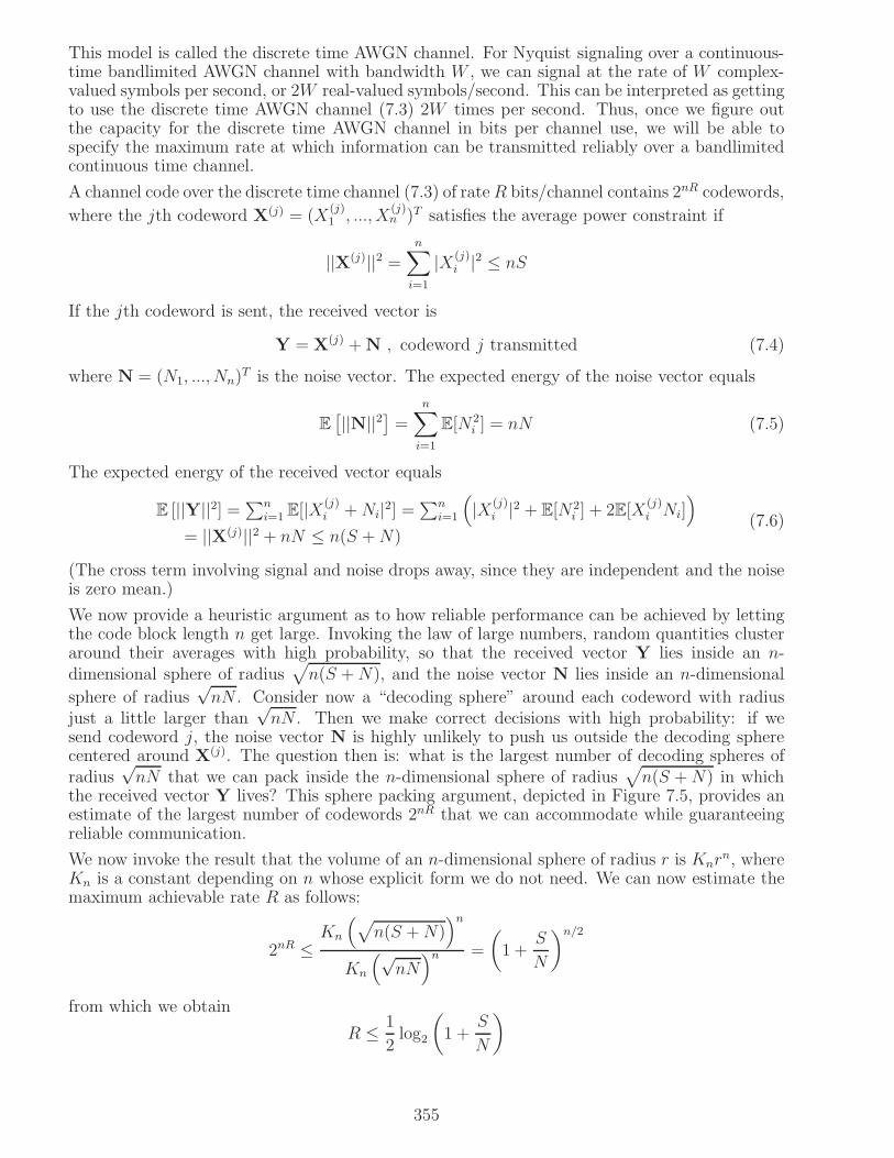
This model is called the discrete time AWGN channel. For Nyquist signaling over a continuous-time bandlimited AWGN channel with bandwidth W , we can signal at the rate of W complex-valued symbols per second, or 2W real-valued symbols/second. This can be interpreted as gettingto use the discrete time AWGN channel (7.3) 2W times per second. Thus, once we figure outthe capacity for the discrete time AWGN channel in bits per channel use, we will be able tospecify the maximum rate at which information can be transmitted reliably over a bandlimitedcontinuous time channel.

A channel code over the discrete time channel (7.3) of rateR bits/channel contains 2nR codewords,

where the jth codeword X(j) = (X(j)1 , ..., X

(j)n )T satisfies the average power constraint if

||X(j)||2 =n∑

i=1

|X(j)i |2 ≤ nS

If the jth codeword is sent, the received vector is

Y = X(j) +N , codeword j transmitted (7.4)

where N = (N1, ..., Nn)T is the noise vector. The expected energy of the noise vector equals

E[

||N||2]

=

n∑

i=1

E[N2i ] = nN (7.5)

The expected energy of the received vector equals

E [||Y||2] =∑ni=1 E[|X

(j)i +Ni|2] =

∑ni=1

(

|X(j)i |2 + E[N2

i ] + 2E[X(j)i Ni]

)

= ||X(j)||2 + nN ≤ n(S +N)(7.6)

(The cross term involving signal and noise drops away, since they are independent and the noiseis zero mean.)

We now provide a heuristic argument as to how reliable performance can be achieved by lettingthe code block length n get large. Invoking the law of large numbers, random quantities clusteraround their averages with high probability, so that the received vector Y lies inside an n-dimensional sphere of radius

√

n(S +N), and the noise vector N lies inside an n-dimensional

sphere of radius√nN . Consider now a “decoding sphere” around each codeword with radius

just a little larger than√nN . Then we make correct decisions with high probability: if we

send codeword j, the noise vector N is highly unlikely to push us outside the decoding spherecentered around X(j). The question then is: what is the largest number of decoding spheres ofradius

√nN that we can pack inside the n-dimensional sphere of radius

√

n(S +N) in whichthe received vector Y lives? This sphere packing argument, depicted in Figure 7.5, provides anestimate of the largest number of codewords 2nR that we can accommodate while guaranteeingreliable communication.

We now invoke the result that the volume of an n-dimensional sphere of radius r is Knrn, where

Kn is a constant depending on n whose explicit form we do not need. We can now estimate themaximum achievable rate R as follows:

2nR ≤Kn

(

√

n(S +N))n

Kn

(√nN)n =

(

1 +S

N

)n/2

from which we obtain

R ≤ 1

2log2

(

1 +S

N

)

355

0

nN

n(S+N)

(j)X ...

Figure 7.5: Sphere packing argument for characterizing rate of reliable communication.

While we have used heuristic arguments to arrive at this result, it can actually be rigorouslydemonstrated that the right-hand side of (7.7) is indeed the maximum possible rate of reliablecommunication over the discrete-time AWGN channel.

Capacity of the discrete time AWGN channel: We can now state that the capacity of thediscrete time AWGN channel (7.3) is given by

Cd−AWGN =1

2log2

(

1 +S

N

)

bits/channel use (7.7)

Continuous time bandlimited AWGN channel: We now use this result to compute themaximum spectral efficiency attainable over a continuous time bandlimited AWGN channel.The complex baseband channel corresponding to a passband channel of physical bandwidth Wspans [−W/2,W/2] (taking the reference frequency at the center of the passband). Thus, Nyquistsignaling over this channel corresponds toW complex-valued symbols per second, or 2W uses persecond of the real-valued channel (7.3). Since each complex-valued symbol corresponds to twouses of the real discrete time AWGN channel, the capacity of the bandlimited channel is given by2WCd−AWGN bits per second. We still need to specify S

N. For each complex-valued sample, the

energy per symbol Es = rEb (bits/symbol, times energy per bit, gives energy per complex-valuedsymbol). The noise variance per real dimension is σ2 = N0

2, hence the noise variance seen by a

complex symbol is 2σ2 = N0. We obtain

S

N=Es

N0(7.8)

Putting these observations together, we can now state the following formula for the capacity ofthe bandlimited AWGN channel.

Capacity of the bandlimited AWGN channel:

CBL

(

W,Es

N0

)

= W log2

(

1 +Es

N0

)

bits per second (7.9)

356

It can be checked that we get exactly the same result for a physical (real-valued) basebandchannel of physical bandwidth W . Such a channel spans [−W,W ], but the transmitted signal isconstrained to be real-valued. Signals over such a channel can therefore be represented by 2Wreal-valued samples per second, which is the same as for a passband channel of bandwidth W .

For a system communicating reliably at a bit rate of Rb bps over such a bandlimited channel,we must have Rb < CBL. Using (7.9), we see that the spectral efficiency r = Rb

Win bps/Hz of the

system must therefore satisfy

r < log2

(

1 +Es

N0

)

= log2

(

1 + rEb

N0

)

bps/Hz or bits/complex symbol (7.10)

where we have used (7.2).

The preceding defines the regime where reliable communication is possible. We can rewrite (7.10)to obtain the fundamental limits on the power-bandwidth tradeoffs achievable over the AWGNchannel, as follows.

0 1 2 3 4 5 6 7−2

0

2

4

6

8

10

12

14

Spectral efficiency r (bps/Hz)

Min

imum

req

uire

d E

b/N

0 (d

B)

Reliable communication possible

Reliable communication not possible

Figure 7.6: Power-bandwidth tradeoffs over the AWGN channel.

Fundamental power-bandwidth tradeoff for the bandlimited AWGN channel:

Eb

N0

>2r − 1

rregime where reliable communication is possible (7.11)

The quantity r is the bandwidth efficiency of a bandlimited AWGN channel. This fundamentalpower-bandwidth tradeoff is depicted in Figure 7.6, which plots the minimum required Eb/N0

(dB) versus the bandwidth efficiency. Note that we cannot make the Eb/N0 required for reliablecommunication arbitrarily small even as the bandwidth efficiency goes to zero. We leave itas an exercise (Problem 7.6) to show that the minimum possible value of Eb/N0 for reliablecommunication (corresponding to r → 0) over the AWGN channel is −1.6 dB. Another pointworth emphasizing is that these power-bandwidth tradeoffs assume powerful channel coding, andare different from those discussed for uncoded systems in Chapter 6: recall that the bandwidthefficiency forM-ary uncoded linear modulation was equal to log2M , and that the power efficiency

was defined asd2min

Eb. Numerical examples showing how channel coding fundamentally changes the

achievable power-bandwidth tradeoffs are explored in more detail in Section 7.3.1. We providehere a quick example that illustrates how (7.11) relates to real world scenarios.

Example 7.3.1 (evaluating system feasibility using Shannon limits) A company claimsto have developed a wireless modem with a receiver sensitivity of -82 dBm and a noise figure of

357

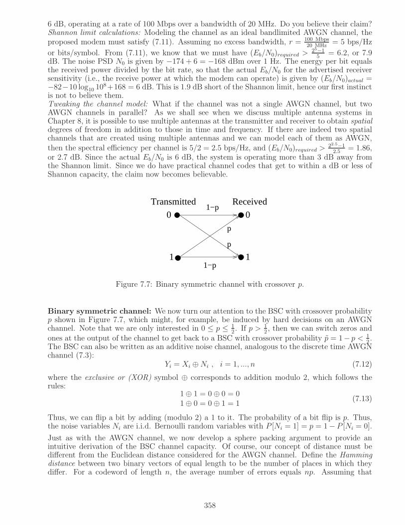
6 dB, operating at a rate of 100 Mbps over a bandwidth of 20 MHz. Do you believe their claim?Shannon limit calculations: Modeling the channel as an ideal bandlimited AWGN channel, theproposed modem must satisfy (7.11). Assuming no excess bandwidth, r = 100 Mbps

20 MHz= 5 bps/Hz

or bits/symbol. From (7.11), we know that we must have (Eb/N0)required >25−15

= 6.2, or 7.9dB. The noise PSD N0 is given by −174 + 6 = −168 dBm over 1 Hz. The energy per bit equalsthe received power divided by the bit rate, so that the actual Eb/N0 for the advertised receiversensitivity (i.e., the receive power at which the modem can operate) is given by (Eb/N0)actual =−82−10 log10 10

8+168 = 6 dB. This is 1.9 dB short of the Shannon limit, hence our first instinctis not to believe them.Tweaking the channel model: What if the channel was not a single AWGN channel, but twoAWGN channels in parallel? As we shall see when we discuss multiple antenna systems inChapter 8, it is possible to use multiple antennas at the transmitter and receiver to obtain spatialdegrees of freedom in addition to those in time and frequency. If there are indeed two spatialchannels that are created using multiple antennas and we can model each of them as AWGN,then the spectral efficiency per channel is 5/2 = 2.5 bps/Hz, and (Eb/N0)required >

22.5−12.5

= 1.86,or 2.7 dB. Since the actual Eb/N0 is 6 dB, the system is operating more than 3 dB away fromthe Shannon limit. Since we do have practical channel codes that get to within a dB or less ofShannon capacity, the claim now becomes believable.

p

Received

0

1

0

1

Transmitted1−p

p

1−p

Figure 7.7: Binary symmetric channel with crossover p.

Binary symmetric channel: We now turn our attention to the BSC with crossover probabilityp shown in Figure 7.7, which might, for example, be induced by hard decisions on an AWGNchannel. Note that we are only interested in 0 ≤ p ≤ 1

2. If p > 1

2, then we can switch zeros and

ones at the output of the channel to get back to a BSC with crossover probability p = 1− p < 12.

The BSC can also be written as an additive noise channel, analogous to the discrete time AWGNchannel (7.3):

Yi = Xi ⊕Ni , i = 1, ..., n (7.12)

where the exclusive or (XOR) symbol ⊕ corresponds to addition modulo 2, which follows therules:

1⊕ 1 = 0⊕ 0 = 01⊕ 0 = 0⊕ 1 = 1

(7.13)

Thus, we can flip a bit by adding (modulo 2) a 1 to it. The probability of a bit flip is p. Thus,the noise variables Ni are i.i.d. Bernoulli random variables with P [Ni = 1] = p = 1− P [Ni = 0].

Just as with the AWGN channel, we now develop a sphere packing argument to provide anintuitive derivation of the BSC channel capacity. Of course, our concept of distance must bedifferent from the Euclidean distance considered for the AWGN channel. Define the Hammingdistance between two binary vectors of equal length to be the number of places in which theydiffer. For a codeword of length n, the average number of errors equals np. Assuming that

358

the number of errors clusters around this average for large n, define a decoding sphere around acodeword as all sequences which are at Hamming distance of np or less from it. The number ofsuch sequences is called the volume of the decoding sphere. By virtue of (7.12) and (7.13), wesee that this volume is exactly equal to the number of noise vectors N = (N1, ..., Nn)

T with npor fewer ones (the number of ones in a sequence is called its weight). The number of n-length

vectors with weight m equals

(

nm

)

, hence the number of vectors with weight at most np is

given by

Vn =

np∑

m=0

(

nm

)

(7.14)

We state without proof the following asymptotic approximation for Vn for large n:

Vn ≈ 2nHB(p) , 0 ≤ p <1

2(7.15)

where HB(·) is the binary entropy function, defined by

HB(p) = −p log2 p− (1− p) log2(1− p) , 0 ≤ p ≤ 1 (7.16)

We plot the binary entropy function in Figure 7.8(a). Note the symmetry around p = 12. This is

because, as mentioned earlier, we can map p > 12to 1− p < 1

2by switching the roles of 0 and 1

at the output.

0 0.1 0.2 0.3 0.4 0.5 0.6 0.7 0.8 0.9 10

0.1

0.2

0.3

0.4

0.5

0.6

0.7

0.8

0.9

1

p

Ent

ropy

(bi

ts/s

ymbo

l)

(a) Binary entropy function

0 0.1 0.2 0.3 0.4 0.5 0.6 0.7 0.8 0.9 10

0.1

0.2

0.3

0.4

0.5

0.6

0.7

0.8

0.9

1

Crossover probability

BS

C C

apac

ity (

bits

/cha

nnel

use

)

(b) BSC capacity

Figure 7.8: The binary entropy function HB(p) and the capacity of a BSC with crossover prob-ability p, given by 1−HB(p).

For a length n code of rate R bits/channel use, the number of codewords equals 2nR. The totalnumber of binary sequences of length n, or the entire volume of the space we are working in, is2n. Thus, if we wish to put a decoding sphere of volume Vn around each codeword, the maximumnumber of codewords we can fit must satisfy

2nR ≤ 2n

Vn≈ 2n

2nHB(p)= 2n(1−HB(p)

which givesR ≤ 1−HB(p)

359

It can be rigorously demonstrated that the right-hand side actually equals the capacity of theBSC. We therefore state this result formally.

Capacity of BSC: The capacity of a BSC with crossover probability p is given by

CBSC(p) = 1−HB(p) bits/channel use (7.17)

The capacity is plotted in Figure 7.8(b). We note the following points.• For p = 1

2, the channel is useless (its output does not depend on the input) and has capacity

zero.• For p > 1

2, we switch zeros and ones at the output to obtain an effective BSC with crossover

probability 1− p, hence CBSC(p) = CBSC(1− p).• For p = 0, 1, the channel is perfect, and the capacity attains its maximum value of 1 bit/channeluse.

7.3.1 Design Implications of Shannon Limits

Since the invention of turbo codes in 1993 and the subsequent rediscovery of LDPC codes, wenow know how to construct random-looking codes that can be efficiently decoded (typically us-ing iterative or message passing methods) and come extremely close to Shannon limits. Such“turbo-like” coded modulation strategies have made, or are making, their way into almost everydigital communication technology, including cellular, WiFi, digital video broadcast, optical com-munication, magnetic recording, and flash memory. Thus, we often summarize the performanceof a practical coded modulation scheme by stating how far away it is from the Shannon limit.Let us discuss what this means via an example. A rate 1

2binary code is employed using bit

interleaved coded modulation with a 16QAM alphabet. We are told that it operates 2 dB awayfrom the Shannon limit at a BER of 10−5. What does this statement mean?

Since we can convey 4 coded bits every time we send a 16QAM symbol, the spectral efficiencyr = 1

2× 4 = 2 bps/Hz, or information bits per symbol: the product of the binary code rate

(number of information bits per coded bit) and the number of coded bits per symbol gives thenumber of information bits per symbol). From (7.11), the minimum possible Eb/N0 is found tobe about 1.8 dB. This is the minimum possible Eb/N0 at which Shannon tells us that error-freeoperation (in the limit of large code blocklengths) is possible at the given spectral efficiency.Of course, any practical strategy at finite blocklength, no matter how large, will not give userror-free operation, hence we declare some value of error probability that we are satisfied with,and evaluate the Eb/N0 for which that error probability is attained. Hence the statement thatwe started with says that our particular coded modulation strategy provides BER of 10−5 atEb/N0 = 1.8 + 2 = 3.8 dB (2 dB higher than the Shannon limit).

How much gain does the preceding approach provide over uncoded communication? Let uscompare it with uncoded QPSK, which has the same spectral efficiency of 2 bps/Hz. The BER

is given by the expression Q(√

2Eb/N0), and we can check that 10−5 BER is attained at Eb/N0

of 9.6 dB. Thus, we get a significant coding gain of 9.6− 3.8 = 5.8 dB from using a sophisticatedcoded modulation strategy, first expanding the constellation from QPSK to 16QAM so there is“room” to insert redundancy, and then using a powerful binary code.

The specific approach for applying a turbo-like coded modulation strategy depends on the systemat hand. For systems with retransmissions (e.g., wireless data), we are often happy with blockerror rates of 1% or even higher, and may be able to use these relatively relaxed specifications tofocus on reducing computational complexity and coding delay (e.g., by considering simpler codesand smaller block lengths). For systems where there is no scope for retransmissions (e.g., storageor broadcast), we may use longer block lengths, and may even layer an outer code to clean up theresidual errors from an inner turbo-like coded modulation scheme. Another common feature ofmany systems is the use of adaptive coded modulation, in which the spectral efficiency is varied

360

as a function of the channel quality. BICM is particularly convenient for this purpose, since itallows us to mix and match a menu of well-optimized binary codes at different rates (e.g., rangingfrom 1

4to 15

16) with a menu of standard constellations (e.g., QPSK, 8PSK, 16QAM, 64QAM) to

provide a large number of options.

A detailed description of turbo-like codes is beyond our present scope, but we do provide adiscussion of decoding via message passing after a basic exposition of linear codes.

7.4 Introducing linear codes

After decades of struggling to construct practical coding strategies that approach Shannon’sperformance limits, we can now essentially declare victory, with channel codes of reasonableblock length coming within less than a dB of capacity. We refer the reader to more advancedtexts and the research literature for details regarding such capacity-achieving codes, and limitourselves here to establishing some basic terminology and concepts which provide a roadmap forfurther exploration. We restrict attention to linear codes, which are by far the most prevalentclass of codes in use today, and suffice to approach capacity. As we discuss shortly, a linear codeis a subspace in a bigger vector space, but the arithmetic we use to define linearity is differentfrom the real- and complex-valued arithmetic we are used to.

Finite fields: We are used to doing calculations with real and complex numbers. The realnumbers, together with the rules of arithmetic, comprise the real field, and the complex numbers,together with the rules of arithmetic, comprise the complex field. Each of these fields hasinfinitely many elements, forming a continuum. However, the basic rules of arithmetic (addition,multiplication, division by nonzero elements, and the associative, distributive and commutativelaws) can also be applied to fields with a finite number of discrete elements. Such fields arecalled finite fields, or Galois fields (after the French mathematician who laid the foundations forfinite field theory). It turns out that, in order to be consistent with the basic rules of arithmetic,the number of elements in a finite field must be a power of a prime, and we denote a finite fieldwith pm elements, where p is a prime, and m a positive integer, as GF (pm). The theory of finitefields, while outside our scope here, is essential for a variety of algebraic code constructions, andwe provide some pointers for further study later in this chapter. Our own discussion here isrestricted to codes over the binary field GF (2).

Binary arithmetic: Binary arithmetic corresponds to operations with only two elements, 0and 1, with addition modulo 2 as specified in (7.13). Binary subtraction is identical to binaryaddition. Multiplication and division (division only permitted by nonzero elements) are trivial,since the only nonzero element is 1. The usual associative, distributive and commutative lawsapply. The elements 0, 1, together with these rules of binary arithmetic, are said to comprisethe binary field GF (2).

Linear binary code: An (n, k) binary linear code C consists of 2k possible codewords, eachof length n, such that adding any two codewords in binary arithmetic yields another codeword.That is, C is closed under linear combinations (the coefficients of the linear combination can onlytake values 0 or 1, since we are working in binary arithmetic), and is therefore a k-dimensionalsubspace of the n-dimensional vector space of all n length binary vectors, in a manner that isentirely analogous to the concept of subspace in real-valued vector spaces. Pursuing this analogyfurther, we can specify a linear code C completely by defining a basis with k vectors, such thatany vector in C (i.e., any codeword) can be expressed as a linear combination of the basis vectors.

Food for thought: The all-zero codeword is always part of any linear code. Why?

Notational convention: While we have preferred working with column vectors thus far, in defer-ence to the convention in most coding theory texts, we express codewords as row vectors. Lettingu and v denote two binary vectors of the same length, we denote by u⊕ v their component by

361

component addition over the binary field. For example, (00110)⊕ (10101) = (10011).

Example 7.4.1 (Repetition code) An (n, 1) repetition code has only two codewords, the all-one codeword x1 = (1, ..., 1) and the all-zero codeword x0 = (0, ..., 0). We see that x1 ⊕ x1 =x0 ⊕ x0 = x0 and that x1 ⊕ x0 = x0 ⊕ x1 = x1, so that this is indeed a linear code. There areonly 21 codewords, so that the dimension k = 1. Thus, the code, when viewed as a vector spaceover the binary field, is spanned by a single basis vector, x1. While the encoding operation istrivial (just repeat the information bit n times) for this code, let us write it in a manner thatleads into a more general formalism. For example, for the (5, 1) repetition code, the informationbit u∈0, 1 is mapped to codeword x as follows:

x = uG

whereG = (1 1 1 1 1) (7.18)

is a matrix whose rows (just one row in this case) provide a basis for the code.

Example 7.4.2 (Single parity check code) An (n, n − 1) single parity check code takes asinput n−1 unconstrained information bits u = (u1, ..., un−1), maps them unchanged to n−1 bitsin the codeword, and adds a single parity check bit to obtain a codeword x = (x1, ..., xn−1, xn).For example, we can set the first n−1 code bits to the information bits (x1 = u1, ..., xn−1 = un−1)and append a parity check bit as follows:

xn = x1 ⊕ x2...⊕ xn−1

Here, the code dimension k = n − 1, so that we can describe the code using n − 1 linearlyindependent basis vectors. For example, for the (5, 4) single parity check code, a particularchoice of basis vectors, put as rows of a matrix as follows:

G =

1 0 0 0 10 1 0 0 10 0 1 0 10 0 0 1 1

(7.19)

We can now check that any codeword can be written as

x = uG

where u = (u1, ..., u4) is the information bit sequence.

Generator matrix: While the preceding examples are very simple, they provide insight intothe general structure of linear codes. An (n, k) linear code can be represented by a basis withk linearly independent vectors, each of length n. Putting these k basis vectors as the rows of ak × n matrix G, we can then define a mapping from k information bits, represented as a 1 × krow vector u, to n code bits, represented as a 1× n row vector x, as follows:

x = uG (7.20)

The matrix G is called the generator matrix for the code, since it can be used to generate all 2k

codewords by cycling through all possible values of the information vector u.

Dual codes: Drawing again on our experience with real-valued vector spaces, we know that,for any k-dimensional subspace C in an n-dimensional vector space, we can find an orthogonaln− k dimensional subspace C⊥ such that every vector in C is orthogonal to every vector in C⊥.The subspace C⊥ is itself an (n, n− k) code, and C and C⊥ are said to be duals of each other.

362

Example 7.4.3 (Duality of repetition and single parity check codes) It can be checkedthat the (5, 4) single parity check code and (5, 1) repetition codes are duals of each other. Thatis, each codeword in the (5, 4) code is orthogonal to each codeword in the (5, 1) code. Sincecodewords are linear combinations of rows of the generator matrix, it suffices to check that eachrow of a generator matrix for the (5, 4) code is orthogonal to each row of a generator matrix forthe (5, 1) code. Specifically,

G(5,1)GT(5,4) = (11111)

1 0 0 00 1 0 00 0 1 00 0 0 11 1 1 1

= 0

Parity check matrix: The preceding discussion shows that we can describe an (n, k) linearcode C by specifying its dual code C⊥. In particular, a generator matrix for the dual code servesas a parity check matrix H for C, in the sense that an n-dimensional binary vector x lies in C ifand only if it is orthogonal to each row of H. That is,

HxT = 0 if and only if x∈C (7.21)

Each row of the parity check matrix defines a parity check equation. Thus, for a parity checkmatrix H of dimension (n − k) × n, each codeword must satisfy n − k parity check equations.Equivalently, if G is a generator matrix for C, then it must satisfy

HGT = 0 (7.22)

In our examples, the generator matrix for the (5, 1) repetition code is a parity check matrix forthe (5, 4) code, and vice versa.

For an (n, k) code with large n and k, it is clearly difficult to check by brute force searchenumeration over 2k codewords whether a particular n-dimensional vector y is a valid codeword.However, for a linear code, it becomes straightforward to verify this using only n−k parity checkequations, as in (7.21). These parity check equations, which provide the redundancy requiredto overcome channel errors, are important not only for verification of correct termination ofdecoding, but also play a crucial role during the decoding process, as we illustrate shortly.

Non-uniqueness: An (n, k) linear code C is a unique subspace consisting of a set of 2k code-words, and its dual (n, n−k) code C⊥ is a unique subspace comprising 2n−k codewords. However,in general, neither the generator nor the parity check matrix for a code are unique, since thechoice of basis for a nontrivial subspace is not unique. Thus, while the generator matrix forthe (5, 1) code is unique because of its trivial nature (one dimension, binary field), the generatormatrix for the (5, 4) code is not. For example, by taking linear combinations of the rows in (7.19),we obtain another linearly independent basis that provides an alternative generator matrix forthe (5, 4) code:

G =

1 1 0 0 00 1 1 0 01 1 1 0 10 1 1 1 1

(7.23)

From (7.20), we see that different choices of generator matrices correspond to different ways ofencoding a k-dimensional information vector u into an n-dimensional codeword x∈C.Systematic encoding: A systematic encoding is one in which the information vector u appearsdirectly in x (without loss of generality, we can take the bits of u to be the first k bits in x), so

363

that there is a clear separation between “information bits” and “parity check” bits. In this case,the generator matrix can be written as

G = [Ik∣

∣P] systematic encoding (7.24)

where Ik denotes the k×k identity matrix, and P is a k×(n−k) matrix specifying how the n−kparity bits depend on the input. The identity matrix ensures that the k rows of G are linearlyindependent, so this does represent a valid generator matrix for an (n, k) code. The ith row ofthe generator matrix (7.24) corresponds to an information vector u = (u1, ..., uk) with ui = 1and uj = 0, j 6= i. Note that, even when we restrict the encoding to be systematic, the generatormatrix is not unique in general. The generator matrices (7.18) and (7.19) for the (5, 1) and (5, 4)codes correspond to systematic encoding. The encoding of the (5, 4) code corresponding to thegenerator matrix in (7.23) is not systematic.

Reading off a parity check matrix from a systematic generator matrix: If we are givena systematic encoding of the form (7.24), we can easily read off a parity check matrix as follows:

H = [−PT∣

∣In−k] (7.25)

where the negative sign can be dropped for the binary field. The identity matrix ensures thatn− k rows of H are linearly independent, hence this is a valid parity check matrix for an (n, k)linear code. We leave it as an exercise to verify, by directly substituting from (7.24) and (7.25),that HGT = 0.

Example 7.4.4 (running example: a (5, 2) linear code) Let us now construct a somewhatless trivial linear code which will serve as a running example for illustrating some basic concepts.Suppose that we have k = 2 information bits u1, u2∈0, 1 that we wish to protect. We mapthis (using a systematic encoding) to a codeword of length 5 using a combination of repetitionand parity check, as follows:

x = (u1, u2, u1, u2, u1 ⊕ u2) (7.26)

A systematic generator matrix for this (5, 2) code can be constructed by considering the twocodewords corresponding to u = (1, 0) and u = (0, 1), respectively, which gives:

G =

(

1 0 1 0 10 1 0 1 1

)

(7.27)

We can read off a parity check matrix using (7.24) and (7.25) to obtain:

H =

1 0 1 0 00 1 0 1 01 1 0 0 1

(7.28)

Any codeword x = (x1, ..., x5) must satisfy HxT = 0, which corresponds to the following paritycheck equations:

x1 ⊕ x3 = 0x2 ⊕ x4 = 0x1 ⊕ x2 ⊕ x3 = 0

Suppose, now, that we transmit the (5, 2) code that we have just constructed over a BSC withcrossover probability p. That is, we send a codeword x = (x1, ..., x5) using the channel n = 5times. According to our discrete memoryless channel model, errors occur independently for eachof the code symbols, and we get the output y = (y1, ..., y5), where P [yi|xi] = xi with probability

364

1 − p, and P [yi|xi] = xi ⊕ 1 (i.e, the bit is flipped) with probability p. How should we try todecode (i.e., estimate which codeword x was sent from the noisy output y)? And how do weevaluate the performance of our decoding rule? In order to relate these to the structure of thecode, it is useful to reiterate the notion of Hamming distance, and to introduce the concept ofHamming weight.

Hamming distance: The Hamming distance dH(u,v) between two binary vectors u and v ofequal length is the number of places in which they differ.For example, the Hamming distance between the two rows of the generator matrix G in (7.27)is given by dH(g1, g2) = 4.

Hamming weight: The Hamming weight wH(u) of a binary vector u equals the number ofones it contains.For example, the Hamming weight of each row of the generator matrix G in (7.27) is 3.

The Hamming distance between two vectors u and v is the Hamming weight of their binary sum:

dH(u,v) = wH(u⊕ v) (7.29)

Structure of an (n, k) linear code: Consider a specific codeword x0 in a linear code C,and consider its Hamming distance from another codeword x∈C. We know that dH(x0,x) =wH(x0 ⊕ x). By linearity, x = x0 ⊕ x is also a codeword in C, and distinct choices of x givedistinct codewords x. Thus, as we run through all possible codewords x∈C, we obtain allpossible codewords x∈C (including x = 0 for x = x0. Thus, dH(x0,x) = wH(x), so that theset of Hamming distances between x0 and all codewords in C (running through all 2k choices ofx) is precisely the set of weights that the codewords in C have (corresponding to the 2k distinctvectors x, one for each x).

Minimum distance: The minimum distance of a code is defined as

dmin = minx1,x2 ∈ C,x1 6=x2dH(x1,x2)

Applying (7.29), and noting that, for a linear code, x1 ⊕ x2 is a nonzero codeword in C, we seethat the minimum distance equals the minimum weight among all nonzero codewords. That is,

dmin = wmin = minx∈ C,x 6=0wH(x) , for a linear code (7.30)

The (5, 2) code is small enough that we can simply list all four codewords: 00000, 10101, 01011,and 11110, from which we see that wmin = dmin = 3.

Guarantees on error correction: A code is guaranteed to correct t errors if

2t+ 1 ≤ dmin (7.31)

It is quite easy to see why. We can set up decoding spheres around any codeword of radius t; fora codeword x, this is all vectors y within Hamming distance t:

Dt(x) = y : dH(y,x) ≤ t

The condition (7.31) guarantees that these decoding spheres do not overlap. Thus, if we make atmost t errors, we are guaranteed that the received vector falls into the unique decoding spherecorresponding to the transmitted codeword.

Erasures: There are some scenarios for which it is useful to introduce the concept of erasures,which correspond to assigning a “don’t know” to a symbol rather than making a hard decision.Using a similar argument as before, we can state that a code is guaranteed to correct t errorsand e erasures if

2t + e+ 1 ≤ dmin (7.32)

365

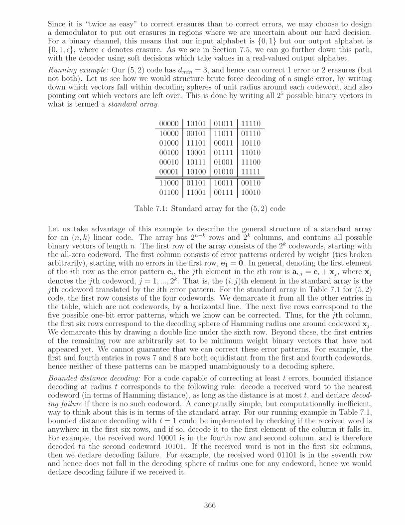
Since it is “twice as easy” to correct erasures than to correct errors, we may choose to designa demodulator to put out erasures in regions where we are uncertain about our hard decision.For a binary channel, this means that our input alphabet is 0, 1 but our output alphabet is0, 1, ǫ, where ǫ denotes erasure. As we see in Section 7.5, we can go further down this path,with the decoder using soft decisions which take values in a real-valued output alphabet.

Running example: Our (5, 2) code has dmin = 3, and hence can correct 1 error or 2 erasures (butnot both). Let us see how we would structure brute force decoding of a single error, by writingdown which vectors fall within decoding spheres of unit radius around each codeword, and alsopointing out which vectors are left over. This is done by writing all 25 possible binary vectors inwhat is termed a standard array.

00000 10101 01011 1111010000 00101 11011 0111001000 11101 00011 1011000100 10001 01111 1101000010 10111 01001 1110000001 10100 01010 11111

11000 01101 10011 0011001100 11001 00111 10010

Table 7.1: Standard array for the (5, 2) code

Let us take advantage of this example to describe the general structure of a standard arrayfor an (n, k) linear code. The array has 2n−k rows and 2k columns, and contains all possiblebinary vectors of length n. The first row of the array consists of the 2k codewords, starting withthe all-zero codeword. The first column consists of error patterns ordered by weight (ties brokenarbitrarily), starting with no errors in the first row, e1 = 0. In general, denoting the first elementof the ith row as the error pattern ei, the jth element in the ith row is ai,j = ei + xj , where xj

denotes the jth codeword, j = 1, ..., 2k. That is, the (i, j)th element in the standard array is thejth codeword translated by the ith error pattern. For the standard array in Table 7.1 for (5, 2)code, the first row consists of the four codewords. We demarcate it from all the other entries inthe table, which are not codewords, by a horizontal line. The next five rows correspond to thefive possible one-bit error patterns, which we know can be corrected. Thus, for the jth column,the first six rows correspond to the decoding sphere of Hamming radius one around codeword xj .We demarcate this by drawing a double line under the sixth row. Beyond these, the first entriesof the remaining row are arbitrarily set to be minimum weight binary vectors that have notappeared yet. We cannot guarantee that we can correct these error patterns. For example, thefirst and fourth entries in rows 7 and 8 are both equidistant from the first and fourth codewords,hence neither of these patterns can be mapped unambiguously to a decoding sphere.

Bounded distance decoding: For a code capable of correcting at least t errors, bounded distancedecoding at radius t corresponds to the following rule: decode a received word to the nearestcodeword (in terms of Hamming distance), as long as the distance is at most t, and declare decod-ing failure if there is no such codeword. A conceptually simple, but computationally inefficient,way to think about this is in terms of the standard array. For our running example in Table 7.1,bounded distance decoding with t = 1 could be implemented by checking if the received word isanywhere in the first six rows, and if so, decode it to the first element of the column it falls in.For example, the received word 10001 is in the fourth row and second column, and is thereforedecoded to the second codeword 10101. If the received word is not in the first six columns,then we declare decoding failure. For example, the received word 01101 is in the seventh rowand hence does not fall in the decoding sphere of radius one for any codeword, hence we woulddeclare decoding failure if we received it.

366

Each row of the standard array is the translation of the code C by its first entry, ei, and is calleda coset of the code. The first entry ei is called the coset leader for the ith coset, i = 1, ..., 2n−k.We now note that a coset can be described far more economically than by listing all its elements.Applying a parity check matrix to the jth element of the ith coset, H(xj ⊕ ei)

T = HeTi , weget an answer that depends only on the coset leader, since HxT = 0 for any codeword x. Wetherefore define the syndrome for the ith coset as si = HeTi . The syndrome is a binary vector oflength n− k, and takes 2n−k possible values. The coset leaders and syndromes corresponding toTable 7.1, using the parity check matrix (7.25), are listed in Table 7.2.

Coset leader Syndrome00000 00010000 10101000 01100100 10000010 01000001 001

11000 11001100 111

Table 7.2: Mapping between coset leaders and syndromes for the (5, 2) code using (7.25)

Bounded distance decoding using syndromes: Consider a received word y. Compute the syndromes = HyT . If the syndrome corresponds to a coset leader e that is within the decoding sphere ofinterest, then we estimate the transmitted codeword as x = y + e. Consider again the receivedword y = 10001 and compute its syndrome s = HyT = 100. This corresponds to the fourthrow in Table 7.2, which we know is within a decoding sphere of radius one. The coset leader ise = 00100. Adding this to the received word, we obtain x = y + e = 10101, which is the sameresult that we obtained by direct look-up in the standard array.

Performance of bounded distance decoding: Correct decoding occurs if the received word ismapped to the transmitted word. For bounded distance decoding with t = 1 for the (5, 2)code, this happens if and only if there is at most one error. Thus, when a codeword for the (5, 2)code is sent over a BSC with crossover probability p, the probability of correct decoding is givenby

Pc = (1− p)5 +

(

51

)

p(1− p)4

If the decoding is not correct, let us term the event incorrect decoding. One of two thingshappen when the decoding is incorrect: the received word falls outside the decoding sphere of allcodewords, hence we declare decoding failure, or the received word falls inside the decoding sphereof one of the incorrect codewords, and we have an undetected error. The sum of the probabilitiesof these two events is Pe = 1 − Pc. Since decoding failure (where we know something has gonewrong) is less damaging than decoding error (where we do not realize that we have made errors),we would like its probability Pdf to be much larger than the probability Pue of undetected error.For large block lengths n, we can typically design codes for which this is possible, hence weoften take Pe as a proxy for decoding failure. For our simple running example, we compute theprobabilities of decoding failure and decoding error in Problem 7.13. Exact computations of Pdf

and Pue are difficult for more complex codes, hence we typically resort to bounds and simulations.

Even when we use syndromes to infer coset leaders rather than searching the entire standardarray, look-up based approaches to decoding do not scale well as we increase the code blocklength n and the decoding radius. A significant achievement of classical coding theory hasbeen to construct codes whose algebraic structure can be exploited to devise efficient meansof mapping syndromes to coset leaders for bounded distance decoding (such methods typically

367

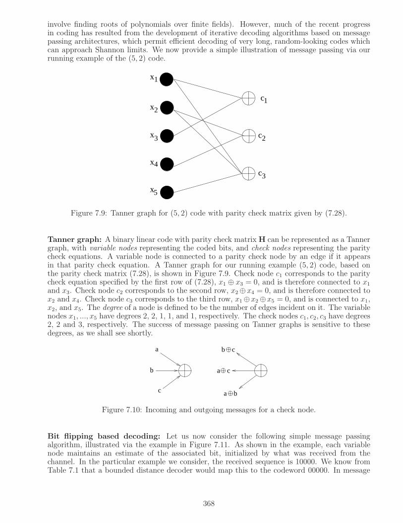
involve finding roots of polynomials over finite fields). However, much of the recent progressin coding has resulted from the development of iterative decoding algorithms based on messagepassing architectures, which permit efficient decoding of very long, random-looking codes whichcan approach Shannon limits. We now provide a simple illustration of message passing via ourrunning example of the (5, 2) code.

1

x2

x3

x4

x5

c1

c2

c3

x

Figure 7.9: Tanner graph for (5, 2) code with parity check matrix given by (7.28).

Tanner graph: A binary linear code with parity check matrix H can be represented as a Tannergraph, with variable nodes representing the coded bits, and check nodes representing the paritycheck equations. A variable node is connected to a parity check node by an edge if it appearsin that parity check equation. A Tanner graph for our running example (5, 2) code, based onthe parity check matrix (7.28), is shown in Figure 7.9. Check node c1 corresponds to the paritycheck equation specified by the first row of (7.28), x1 ⊕ x3 = 0, and is therefore connected to x1and x3. Check node c2 corresponds to the second row, x2⊕x4 = 0, and is therefore connected tox2 and x4. Check node c3 corresponds to the third row, x1⊕x2⊕x5 = 0, and is connected to x1,x2, and x5. The degree of a node is defined to be the number of edges incident on it. The variablenodes x1, ..., x5 have degrees 2, 2, 1, 1, and 1, respectively. The check nodes c1, c2, c3 have degrees2, 2 and 3, respectively. The success of message passing on Tanner graphs is sensitive to thesedegrees, as we shall see shortly.

c

b c

a c

a b

a

b

Figure 7.10: Incoming and outgoing messages for a check node.

Bit flipping based decoding: Let us now consider the following simple message passingalgorithm, illustrated via the example in Figure 7.11. As shown in the example, each variablenode maintains an estimate of the associated bit, initialized by what was received from thechannel. In the particular example we consider, the received sequence is 10000. We know fromTable 7.1 that a bounded distance decoder would map this to the codeword 00000. In message

368

passing for bit flipping, each variable node sends out its current bit estimate on all outgoingedges. Each check node uses these incoming messages to generate new messages back to thevariable nodes, as illustrated in Figure 7.10, which shows a check node of degree 3. That is, themessage sent back to a variable node is the value that bit should take in order to satisfy thatparticular parity check, assuming that the messages coming in from the other variable nodesare correct. When the variable nodes get these messages, they flip their bits if ”enough” checknode messages tell them to. In our example of a (5, 2) code, let us employ the following rule: avariable node flips its channel bit if (a) all the check messages coming into it tell it to, and (b)the number of check messages is more than one (so as to provide enough evidence to overridethe current estimate).

Figure 7.11 shows how bit flipping can be used to correct the one-bit error pattern 10000. Bothcheck node messages to variable node x1 say that it should take value 0, and cause it to flipto the correct value. On the other hand, Figure 7.12 shows that bit flipping gets stuck for theone bit error pattern 00001, because there is only one check message coming into variable nodex5, which is not enough to flip it. Note that both of these error patterns are correctable usingbounded distance decoding, using Table 7.1 or Table 7.2. This reveals an important property ofiterative decoding on Tanner graphs: its success depends critically on the node degrees, which ofcourse depend on the particular choice of parity check matrix used to specify the Tanner graph.

0

c1

c2

c3

x1

x2

x3

x4

x5

c1

c2

c3

x1

x2

x3

x4

x5

1

0

0

0

0

0

0

1

1

1

1

0

Flip this bit

Leave unchanged

1

0

0

0

0

1

1

0

0

0

0

Figure 7.11: Bit flipping based decoding for the (5, 2) code is successful for this error pattern.

Can we fix the problem revealed by the example in Figure 7.12? Perhaps we can choose a differentparity check matrix for which the Tanner graph has variable nodes of degree at least 2, so thatbit flipping has a chance of working? For codes over large block lengths, it is actually possibleto use a randomized approach for the design of parity check matrices yielding desirable degreedistributions, enabling spectacular performance approaching Shannon limits. In these regimes,iterative decoding goes well beyond the error correction capability guarantees associated withthe code’s minimum distance. However, such results do not apply to the simple example we areconsidering, where iterative decoding is having trouble decoding even up to the guarantee of t = 1associated with a minimum distance dmin = 3. However, this gives us the opportunity to presenta trick that can be useful even for large block lengths: use redundant parity check nodes, addingone or more rows to the parity check matrix that are linearly dependent on other rows. Figure7.13 shows a Tanner graph for the (5, 2) code with a redundant check node c4 corresponding tox3 ⊕ x4 ⊕ x5 = 0. That is, we have added a fourth row 00111 to the parity check matrix (7.25).This row is actually a sum of the first three rows, and hence would add no further informationif we were just performing look-up based bounded distance decoding. However, revisiting thetroublesome error pattern 00001, we see that this redundant check makes all the difference inthe performance of bit flipping based decoding; as Figure 7.14 shows, the pattern can now be

369

0

c1

c2

c3

x1

x2

x3

x4

x5

c1

c2

c3

x1

x2

x3

x4

x5

0

0

1

00

0

0 0

0

0

0

0

1

0

0

1

0

0

0

1

1

0

All bits remain unchanged

0

Figure 7.12: Bit flipping based decoding for the (5, 2) code is unsuccessful for this error pattern,even though it is correctable using bounded distance decoding.

corrected.

(redundant parity check)

1

x2

x3

x4

x5

c1

c2

c3

c4

x

Figure 7.13: Tanner graph for (5, 2) code with one redundant parity check.

7.5 Soft decisions and belief propagation

We have discussed decoding of linear block codes based on hard decision inputs, where the inputto the decoder is a string of bits. However, these bits are sent over a channel using modulationtechniques such as those discussed in Chapter 4, and as discussed in Chapter 6, it is possible toextract soft decisions that capture more of the information we have about the physical channel.In this section, we discuss how soft decisions can be used in iterative decoding, illustrating thekey concepts using our running example (5, 2) code. We restrict attention to BPSK modulationover a discrete-time AWGN channel, but as the discussion in Chapter 6 indicates, the conceptof soft decisions is applicable to any signaling scheme.

A codeword x = (x[1], ..., x[n]) with elements taking values in 0, 1 can be mapped to a sequence

370

unchanged

c1

c2

c3

x1

x2

x3

x4

x5

c1

c2

c3

x1

x2

x3

x4

x5

c4 c4

0

0

0

0

1

00

0

0

0

0

0

0

1

0

0

0

0

1

1

0

1

0

0

1

00

0

1

1

Flip this bit

These bits remain

Figure 7.14: Bit flipping based decoding for the (5, 2) code using a redundant parity check isnow successful for the 00001 error pattern.

of BPSK symbols using the transformation

b[m] = (−1)x[m] , m = 1, ..., n (7.33)

The advantage of this map is that it transforms binary addition into real-valued multiplication.That is, x[m1]⊕ x[m2] maps to b[m1]b[m2]. The BPSK symbols are transmitted over a discretetime AWGN channel, with received symbols given by

y[m] = Ab[m] + w[m] = A(−1)x[m] + w[m] , m = 1, ..., n (7.34)

where the amplitude A =√Es, where Es denotes the energy/symbol, and w[m] ∼ N(0, σ2)

are i.i.d. discrete time WGN samples. To simplify notation, consider a single bit x∈0, 1,mapped to b∈−1,+1, with received sample y = Ab+w, w ∼ N(0, σ2). Consider the posteriorprobabilities P [x = 0|y] and P [x = 1|y]. Since P [x = 0|y] + P [x = 1|y] = 1, we can conveyinformation regarding these probabilities in a number of ways. One particularly convenientformat is the log likelihood ratio (LLR), defined as

L(x) = logP [x = 0]

P [x = 1]= log

P [b = +1]

P [b = −1](7.35)

where we omit the conditioning on y to simplify notation. We can go from LLRs to bit proba-bilities as follows:

P [x = 0] =eL(x)

eL(x) + 1, P [x = 1] =

1

eL(x) + 1(7.36)

We can go from LLRs to hard decisions as follows:

b = sign(L) , x = IL<0 = Ib<0 (7.37)

where b∈−1,+1 is the “BPSK” version of x∈0, 1.Suppose that the prior probability of bit x taking value 0 is π0(x). This notation implies that theprior probability could vary across bits: while we do not need this for the examples consideredhere, allowing this level of generality is useful for some decoder structures, such as for turbocodes, the information about bit x supplied by a given decoder component may be interpreted

371

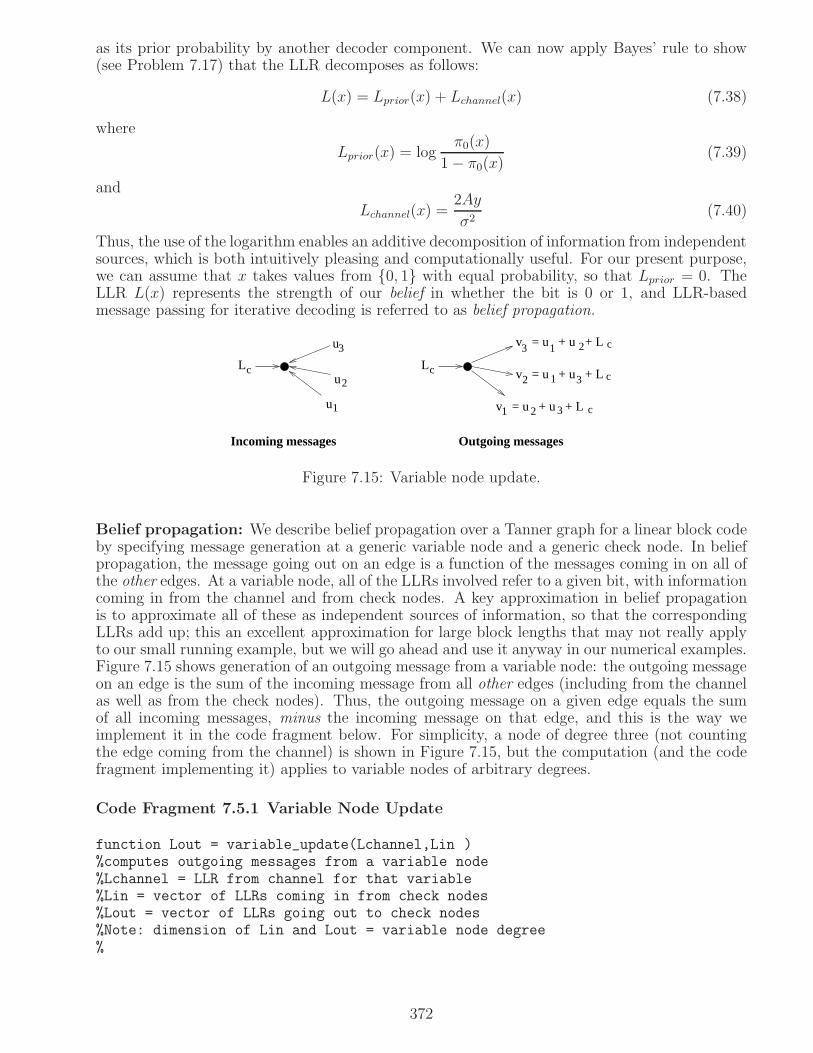
as its prior probability by another decoder component. We can now apply Bayes’ rule to show(see Problem 7.17) that the LLR decomposes as follows:

L(x) = Lprior(x) + Lchannel(x) (7.38)

where

Lprior(x) = logπ0(x)

1− π0(x)(7.39)

and

Lchannel(x) =2Ay

σ2(7.40)

Thus, the use of the logarithm enables an additive decomposition of information from independentsources, which is both intuitively pleasing and computationally useful. For our present purpose,we can assume that x takes values from 0, 1 with equal probability, so that Lprior = 0. TheLLR L(x) represents the strength of our belief in whether the bit is 0 or 1, and LLR-basedmessage passing for iterative decoding is referred to as belief propagation.

Incoming messages

3

u2

u1

Lc Lc

v = u + u + L1 2 3 c

v = u + u + L2 1 3 c

v = u + u + L3 1 2 c

Outgoing messages

u

Figure 7.15: Variable node update.

Belief propagation: We describe belief propagation over a Tanner graph for a linear block codeby specifying message generation at a generic variable node and a generic check node. In beliefpropagation, the message going out on an edge is a function of the messages coming in on all ofthe other edges. At a variable node, all of the LLRs involved refer to a given bit, with informationcoming in from the channel and from check nodes. A key approximation in belief propagationis to approximate all of these as independent sources of information, so that the correspondingLLRs add up; this an excellent approximation for large block lengths that may not really applyto our small running example, but we will go ahead and use it anyway in our numerical examples.Figure 7.15 shows generation of an outgoing message from a variable node: the outgoing messageon an edge is the sum of the incoming message from all other edges (including from the channelas well as from the check nodes). Thus, the outgoing message on a given edge equals the sumof all incoming messages, minus the incoming message on that edge, and this is the way weimplement it in the code fragment below. For simplicity, a node of degree three (not countingthe edge coming from the channel) is shown in Figure 7.15, but the computation (and the codefragment implementing it) applies to variable nodes of arbitrary degrees.

Code Fragment 7.5.1 Variable Node Update

function Lout = variable_update(Lchannel,Lin )%computes outgoing messages from a variable node%Lchannel = LLR from channel for that variable%Lin = vector of LLRs coming in from check nodes%Lout = vector of LLRs going out to check nodes%Note: dimension of Lin and Lout = variable node degree%

372

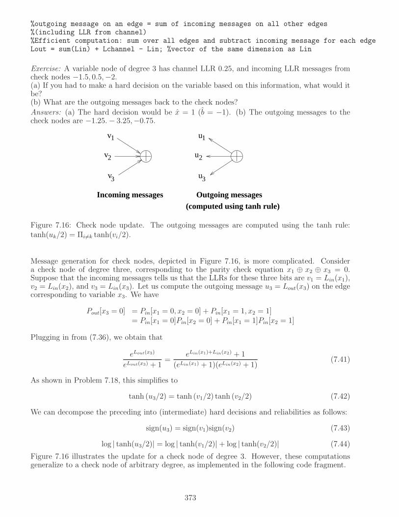
%outgoing message on an edge = sum of incoming messages on all other edges%(including LLR from channel)%Efficient computation: sum over all edges and subtract incoming message for each edgeLout = sum(Lin) + Lchannel - Lin; %vector of the same dimension as Lin

Exercise: A variable node of degree 3 has channel LLR 0.25, and incoming LLR messages fromcheck nodes −1.5, 0.5,−2.(a) If you had to make a hard decision on the variable based on this information, what would itbe?(b) What are the outgoing messages back to the check nodes?

Answers: (a) The hard decision would be x = 1 (b = −1). (b) The outgoing messages to thecheck nodes are −1.25.− 3.25,−0.75.

Incoming messages

v1

v2

v3

1u

2u

3u

Outgoing messages(computed using tanh rule)

Figure 7.16: Check node update. The outgoing messages are computed using the tanh rule:tanh(uk/2) = Πi 6=k tanh(vi/2).

Message generation for check nodes, depicted in Figure 7.16, is more complicated. Considera check node of degree three, corresponding to the parity check equation x1 ⊕ x2 ⊕ x3 = 0.Suppose that the incoming messages tells us that the LLRs for these three bits are v1 = Lin(x1),v2 = Lin(x2), and v3 = Lin(x3). Let us compute the outgoing message u3 = Lout(x3) on the edgecorresponding to variable x3. We have

Pout[x3 = 0] = Pin[x1 = 0, x2 = 0] + Pin[x1 = 1, x2 = 1]= Pin[x1 = 0]Pin[x2 = 0] + Pin[x1 = 1]Pin[x2 = 1]

Plugging in from (7.36), we obtain that

eLout(x3)

eLout(x3) + 1=

eLin(x1)+Lin(x2) + 1

(eLin(x1) + 1)(eLin(x2) + 1)(7.41)

As shown in Problem 7.18, this simplifies to

tanh (u3/2) = tanh (v1/2) tanh (v2/2) (7.42)

We can decompose the preceding into (intermediate) hard decisions and reliabilities as follows:

sign(u3) = sign(v1)sign(v2) (7.43)

log | tanh(u3/2)| = log | tanh(v1/2)|+ log | tanh(v2/2)| (7.44)

Figure 7.16 illustrates the update for a check node of degree 3. However, these computationsgeneralize to a check node of arbitrary degree, as implemented in the following code fragment.

373

Code Fragment 7.5.2 Check Node Update

function Lout = check_update( Lin )%computes messages going out from a check node%Lin = vector of messages coming in from variable nodes%Lout = vector of messages going out to variable nodes%convert LLRs to reliabilities and signsreliabilities_in = log(abs(tanh(Lin/2)));signs_in = sign(Lin);%compute check updatereliabilities_out = sum(reliabilities_in) - reliabilities_in;sign_product = prod(signs_in);signs_out = sign_product.*signs_in;%convert reliabilities and signs back to LLRsLout = 2*atanh(exp(reliabilities_out)).*signs_out;

Exercise: A check node of degree 4 has incoming LLRs −3.5, 2.2, 0.25, 1.3.(a) Is the check satisfied by the incoming messages? That is, if we made hard decisions based onthe incoming LLRs, would they satisfy the parity check equation corresponding to this node?(b) Use code fragment 7.5.2 to determine the corresponding outgoing LLRs. How are the signsand reliabilities of the outgoing LLRs related to those of the incoming messages?Answers: (a) No. (b) The outgoing LLRs are 0.1139,−0.1340,−0.9217,−0.1880. The signs areflipped, and the larger reliabilities become smaller, while the smallest reliability increases. Whydoes this make sense?

Once we have defined the computations at the variable and check nodes, all that is needed toimplement belief propagation is to route messages according to the edges defined by a givenparity check matrix (of course, the choice of code and parity check matrix determines whetheriterative decoding is effective). At any stage of iterative decoding, we can make hard decisionsat a variable node using (7.37), where the LLR is the sum of all incoming LLRs, includingthe channel LLR. If the resulting estimated vector x satisfies Hx = 0, then we know that wehave obtained a valid codeword and we can terminate the decoding. Typically, if we do notobtain a valid codeword after a specified number of iterations, then we declare decoding failure.We implement belief propagation based iterative decoding in Software Lab 7.1; while we use ourrunning example (5, 2) code, the software developed in this lab provides a generic implementationof belief propagation for any linear block code once the parity check matrix is specified.

7.6 Concept inventory on channel coding

This section provides a glimpse of channel coding concepts, including fundamental performancelimits established by Shannon theory and constructive strategies for approaching these limits.Key points are summarized as follows.

• The need for non-trivial channel codes is motivated by examining two extremes when sendinga block of bits over a binary symmetric channel: uncoded communication (probability of packeterror tends to one as blocklength increases) and repetition coding (the code rate tends to zeroas blocklength increases).• Channel coding consists of introducing structured redundancy in the transmitted bits/symbols.While there are many possible coded modulation strategies, we focus on BICM, a simple, flexible,and effective approach cascading a binary code and an interleaver, followed by mapping of bitsto modulated symbols.

Shannon limits• For a given channel (fixing parameters such as power and bandwidth), Shannon theory tells us

374

that there is a well-defined maximum possible rate of reliable communication, termed the channelcapacity. For a passband bandlimited AWGN channel with bandwidth W (Hz), the capacity isgiven by W log2 (1 + Es/N0), which translates to the following fundamental power-bandwidthtradeoff:

Es/N0 > 2r − 1, Eb/N0 >2r − 1

r

where Es is the energy per transmitted symbol, Eb is the energy per information bit, and r is thespectral efficiency (the information bit rate normalized by the bandwidth). These results werederived after first showing that the capacity of a discrete time real AWGN channel is given by12log2(1 + S/N) bits per channel use.

• The channel capacity for a BSC with crossover probability p is 1 − HB(p) = 1 + p log2 p +(1− p) log2(1− p) bits per channel use. For BICM, such a channel is obtained, for example, bymaking hard decisions on Gray coded constellations.• Shannon limits can be used for guidelines for choosing system sizing: for example, the combi-nation of code rate and constellation size that is appropriate for a given SNR.• The performance of a given coded modulation strategy can be compared to fundamental limitsby comparing the SNR at which it attains a certain performance (e.g., a BER of 10−5) with theminimum SNR required for reliable communication at that spectral efficiency.

Linear codes• Linear codes are a popular and well-understood design choice in modern communication sys-tems. The 2k codewords in an (n, k) binary linear code C form a k-dimensional subspace of thespace of n-dimensional binary vectors, under addition and multiplication over the binary field.The dual code C⊥ is an (n, n− k) linear code such that each codeword in C is orthogonal (underbinary inner products) to each codeword in C⊥.• A basis for an (n, k) linear code C can be used to form a generator matrix G. A k-dimensionalinformation vector u can be encoded into an n-dimensional codeword x using the generator ma-trix: x = uG.• A basis for the dual code C⊥ can be used to form a parity check matrix H satisfying HxT = 0for any x∈C.• The choices for G and H are not unique, since the choice of basis for a linear vector space isnot unique. Furthermore, we may add redundant rows to H to aid in decoding.• The number of errors t that a code can be guaranteed to correct satisfies 2t+ 1 ≤ dmin, wheredmin is the minimum Hamming distance between codewords. For a linear code, dmin equals theminimum weight among nonzero codewords, since the all-zero vector is always a codeword, andsince the difference between codewords is a codeword.• The translation of codewords by error vectors can be enumerated in a standard array, whoserows correspond to translations of the entire code, termed cosets, by a given error pattern, termedcoset leader. A more compact representation lists only coset leaders and syndromes, obtainedby operating the parity check matrix on a given received word. These can be used to carry outa look-up based implementation of bounded distance decoding.

Tanner graphs• An (n, k) linear code with n × r (r ≥ n − k) parity check matrix H can be represented by aTanner graph, with n variable nodes on one side, and r check nodes on the other side, with anedge between the jth variable and ith check node if and only if H(i, j) = 1.• Message passing on the Tanner graph can be used for iterative decoding, which scales wellto very large code block lengths. One approach is to employ bit flipping algorithms with harddecision inputs and binary messages, but a more powerful approach is to use soft decisions andbelief propagation.

Soft decisions and belief propagation• The messages passed between the variable and check nodes are the bit LLRs. The messagegoing out on an edge depends on the messages coming in on all the other edges.

375

• Outgoing messages from a variable node are generated simply by summing LLRs. Outgoingmessages from a check node are more complicated, but can be viewed as a product of signs, anda sum of reliabilities.

7.7 Endnotes

The material in this chapter has been selected to make two points: (a) information theoryprovides fundamental performance benchmarks that can be used to guide parameter selectionfor communication links; (b) coding theory provides constructive strategies for approaching thesefundamental benchmarks. We now list some keywords associated with topics that a systematicexposition of information and coding theory might cover, and then provide some references forfurther study.

Keywords: A systematic study of information theory, and its application to derive theorems insource and channel coding, includes concepts such as entropy, mutual information, divergenceand typicality. A systematic study of the structure of algebraic codes, such as BCH and RS codes,is required to understand their construction, their distance properties and decoding algorithmssuch as the Berlekamp-Massey algorithm. A study of convolutional codes, their decoding usingthe Viterbi algorithm, and their performance analysis, is another important component of astudy of channel coding. Tight integration of convolutional codes with modulation leads totrellis coded modulation. Suitably interleaving convolutional codes leads to turbo codes, whichcan be decoded iteratively using the forward-backward, or BCJR, algorithm. LDPC codes, whichcan be decoded iteratively by message passing over a Tanner graph (as described here and insoftware lab 7.1), are of course an indispensable component in modern communication design.

Further reading: One level up from the glimpse provided here is a self-contained introductionto “just enough” information theory to compute performance benchmarks for communicationsystems, and a selection of constructive coding and decoding strategies (including convolutional,turbo, and LDPC codes), in the author’s graduate text [7] (Chapters 6 and 7). The textbookby Cover and Thomas [36] is highly recommended for a systematic and lucid exposition ofinformation theory. Shannon’s beautifully written work [37] establishing the field is also highlyrecommended as a source of inspiration. The textbook by McEliece [38] is a good source for a firstexposure to information theory and algebraic coding. A detailed treatment of algebraic codingis provided by the textbook by Blahut [39], while comprehensive treatments of channel coding,including both algebraic and turbo-like codes, are provided in the texts by Lin and Costello [40]and Moon [41].

7.8 Problems

Shannon limits

Problem 7.1 Consider a coded modulation strategy pairing a rate 14binary code with QPSK.

Assuming that this scheme performs 1.5 dB away from the Shannon limit, what are the minimumvalues of Es/N0 (dB) and Eb/N0 (dB) required for the scheme to work?

Problem 7.2 At BER of 10−5, how far away are the following uncoded constellations fromthe corresponding Shannon limits: QPSK, 8PSK, 16QAM, 64QAM. Use the nearest neighborsapproximation for BER of Gray coded constellations in Section 6.4.

Problem 7.3 Consider Gray coded QPSK, 8PSK, 16QAM, and 64QAM.(a) Assuming that we make ML hard decisions, use the nearest neighbors approximation for

376

BER of Gray coded constellations in Section 6.4 to plot the BER as a function of Es/N0 (dB)for each of these constellations.(b) The hard decisions induce a BSC with crossover probability given by the BERs computed in(a). Using the BSC capacity formula (7.17), plot the capacity in bits per symbol as a functionof Es/N0 (dB) for each constellation. Also plot for comparison the capacity of the bandlimitedAWGN channel given by (). Comment on the penalty for hard decisions, as well as any othertrends that you see.

Problem 7.4 Consider a BICM system employing a rate 23binary code with Gray coded QPSK

modulation.(a) What is Es/N0 in terms of Eb/N0?(b) Based on the AWGN capacity region (7.11), what is the Shannon limit for this system (i.e.,the minimum required Eb/N0 in dB)?(c) Now, consider the suboptimal strategy of making hard decisions, thus inducing a BSC. Whatis the Shannon limit for the system? What is the degradation in dB due to making hard decisions?Hint: Hard decisions on Gray coded QPSK symbols induce a BSC with crossover probability

p = Q(

√

2Es/N0

)

, whose capacity is given by (7.17). The Shannon limit is the minimum value

of Eb/N0 for the capacity to be larger than the code rate being used.

Problem 7.5 A rate 1/2 binary code is employed using bit interleaved coded modulation withQPSK, 16QAM, and 64QAM.(a) What are the bit rates attained by these three schemes when operating over a passbandchannel of bandwidth 10 MHz (ignore excess bandwidth).(b) Assuming that each coded modulation scheme operates 2 dB from the Shannon limit, whatis the minimum value of Es/N0 (dB) required for each of the three schemes to provide reliablecommunication?(c) Assuming that these three schemes are employed in an adaptive modulation strategy whichadapts the data rate as a function of the range. Assuming that the largest attainable rangeamong the three schemes is 10 km. Assuming inverse square path loss, what are the rangescorresponding to the other two schemes.(d) Now, if we add binary codes of rate 2

3and 3

4, plot the attainable bit rate versus range for

an adaptive modulation scheme allowing all possible pairings of code rates and constellations.Assume that each scheme is 2 dB away from the corresponding Shannon limit.

Problem 7.6 (a) Apply L’Hospital’s rule to evaluate the limit of the right-hand side of (7.11) asr → 0. What is the minimum possible Eb/N0 in dB at which reliable communication is possibleover the AWGN channel?(b) Re-plot the region for reliable communication shown in Figure 7.6, but this time with spectralefficiency r (bps/Hz) versus the SNR Es/N0 (dB). Is there any lower limit to Es/N0 below whichreliable communication is not possible? If so, what is it? If not, why not?

Linear codes and bounded distance decoding

Problem 7.7 A parity check matrix for the (7, 4) Hamming code is given by

H =

1 0 0 1 0 1 10 1 0 1 1 0 10 0 1 0 1 1 1

(7.45)

(a) Find a generator matrix for the code.(b) Find the minimum distance of the code. How many errors can be corrected using bounded

377

distance decoding?Answer: dmin = 3, hence a bounded distance decoder can correct one error.(c) Write down the standard array. Comment on how any structural differences you see betweenthis and the standard array for the (5, 2) code in Table 7.1.Answer: Unlike in Table 7.1, no binary vectors are “left over” after running through the singleerror patterns. The Hamming code is a perfect code: the decoding spheres of radius one coverthe entire space of length-7 binary vectors. “Perfect” in this case just refers to how well decodingspheres can be packed into the available space; it definitely does not mean “good,” since theHamming code is a weak code.(d) Write down the mapping between coset leaders and syndromes for the given parity checkmatrix (as done in Table 7.2 for the (5, 2) code).

Problem 7.8 Suppose that the (7, 4) Hamming code is used over a BSC with crossover proba-bility p = 0.01. Assuming that bounded distance decoding with decoding radius one is employed,find the probability of correct decoding, the probability of decoding failure, and the probabilityof undetected error.

Problem 7.9 Append a single parity check to the (7, 4) Hamming code. That is, given acodeword x = (x1, ..., x7) for the (7, 4) code, define a new codeword z = (x1, ..., x7, x8) byappending a parity check on the existing code bits:

x8 = x1 ⊕ x2 ⊕ ...⊕ x7

This new code is called an extended Hamming code.(a) What are n and k for the new code?(b) What is the minimum distance for the new code?

Problem 7.10 Hamming codes of different lengths can be constructed using the following pre-scription: the parity check matrix consists of all nonzero binary vectors of length m, where m isa positive integer.(a) What is the value of m for the (7, 4) Hamming code?(b) For arbitrary m, what are the values of code block length n and the number of informationbits k as a function of m?Hint: The code block length is the number of columns in the parity check matrix. The dimensionof the dual code is the rank of the parity check matrix. Remember that row rank equals thecolumn rank. Which is easier to find in this case?

Problem 7.11 BCH codes (named after their discoverers, Bose, Ray-Chaudhury, and Hoc-quenghem) are a popular class of linear codes with a well-defined algebraic structure and well-understood algorithms for bounded distance coding. For a positive integer m, we can constructa binary BCH code which can correct at least t errors with the following parameters:

n = 2m − 1, k ≥ n−mt, dmin ≥ 2t+ 1 (7.46)

so that the code rate R = kn≥ 1− mt

2m−1, where the inequality for k is often tight for small values

of t. For example, Hamming codes are actually (2m − 1, 2m − 1−m) BCH codes with t = 1.Remark: The price of increasing the block length of a BCH code is decoding complexity. Algebraicdecoding of a code of length n = 2m − 1 requires operations over GF (2m).(a) Consider a (1023, 923) BCH code. Assuming that the inequality for k is tight, how manyerrors can it correct?Answer: t = 10.(b) Assuming that the inequality for k in (7.46) is tight, what is the rate of a BCH code withn = 511 and t = 10?

378

Problem 7.12 Consider an (n, k) linear code used over a BSC channel with crossover probabilityp. The number of errors among n code bits is X ∼ Bin(n, p). A bounded distance decoder ofradius t is used to decode it (assume that the code is capable of correcting at least t errors). Theprobability of incorrect decoding is therefore given by

Pe = P [X > t] =n∑

k=t+1

(

nk

)

pk(1− p)n−k (7.47)

The computation in (7.47) is straightforward, but for large n, numerical problems can arise when

evaluating the terms in the sum directly, because

(

nk

)

can take very large values, and pk can

take very small values. One approach to alleviate this problem is to compute the binomial pmfrecursively.(a) Show that

P [X = k] =p

1− p

n− k + 1

kP [X = k − 1] , k = 1, ..., n (7.48)

(b) Use the preceding, together with the initial condition P [X = 0] = (1−p)n, to write a Matlabprogram to compute P [X > t].

Problem 7.13 Use the standard array in Table 7.1 for an exact computation of the probabilitiesof decoding failure and decoding error for the (5, 2) code, for bounded distance decoding witht = 1 over a BSC with crossover probability p. Plot these probabilities as a function of p on alog-log scale.Hint: Assume that the all-zero codeword is sent. Find the number and weight of error patternsresulting in decoding failure and decoding error, respectively

Problem 7.14 For the binomial tail probability (7.47) associated with the probability of incor-rect decoding, we are often interested in large n and relatively small t; for example, consider the(1023, 923) BCH code in Problem 7.11, for which t = 10. While recursive computations as inProblem 7.12 are relatively numerically stable, we are often interested in quick approximationsthat do not require the evaluation of a large summation with (n− t) terms. In this problem, wediscuss some simple approximations.(a) We are interested in designing systems to obtain small values of Pe, hopefully significantlysmaller than the input BER p. Argue that p ≥ t

nis an uninteresting regime from this point of

view. What is the uninteresting regime for the (1023, 923) BCH code?(b) For p≪ t

n, argue that the sum in (7.47) is well approximated by its first term.

(c) Since X is a sum of n i.i.d. Bernoulli random variables, show that the CLT can be used toapproximate its distribution by a Gaussian: X ∼ N(np, np(1− p)).(d) For the (1023, 923) BCH code, compute a numerical estimate of the probability of incorrectdecoding for t = 10 and p = 10−3 in three different ways: (i) direct computation, (ii) estimationby the first term as in (b), (iii) estimation using the Gaussian approximation.(e) Repeat (d) for p = 10−4.(f) Comment on the match (or otherwise) between the three estimates in (d) and (e). Whathappens with smaller p?

Problem 7.15 Here are the (n, k, t) parameters for some other binary BCH codes for which thecomputations of Problem 7.12 can be repeated: (1023, 863, 16), (511, 421, 10), (255, 215, 5).

Problem 7.16 Reed-Solomon (RS) codes are a widely used class of codes on non-binary alpha-bets. While we do not discuss the algebraic structure of any of the codes we have mentioned, we

379

state in passing that RS codes can be viewed as a special class of BCH codes. The symbols inan RS code come from GF (2m) (a finite field with 2m elements, where m is a positive integer),hence each symbol can be represented by m bits. The code block length equals n = 2m− 1. Theminimum distance is given by

dmin = n− k + 1 (7.49)

This is actually the best possible minimum distance attainable for an (n, k) code. It is possibleto extend the RS code by one symbol to obtain n = 2m, and to shorten the code to obtainn < 2m − 1, all the while maintaining the minimum distance relationship (7.49). Boundeddistance decoding can be used to correct up to ⌊dmin−1

2⌋ = ⌊n−k

2⌋ or dmin − 1 = n− k erasures,

or any pattern of t errors and e erasures satisfying 2t+ e+1 ≤ dmin = n− k+1. One drawbackof RS codes: it is not possible to obtain code block lengths larger than 2m, the alphabet size.(a) What is the maximum number of symbol errors that a (255, 235) RS code can correct? Howmany bits does each symbol represent? In the worst case, how many bits can the code correct?How about in the best case?(b) The (255, 235) RS code is used as an outer code in a system in which the inner code producesa BER of 10−3. What is the symbol error probability, assuming that the bit errors are i.i.d.?Assuming bounded distance decoding up to the maximum possible number of correctable errors,find the probability of incorrect decoding.Note: The symbol error probability p = 1− (1 − pb)

m, where pb is the BER and m the numberof bits per symbol.(c) What is the BER that the inner code must produce in order for the (255, 235) RS code toattain a decoding failure probability of less than 10−12?(d) If the BER of the inner code is fixed at 10−3 and the block length and alphabet size of theRS code are as in (b)-(c), what is the value of k for which the decoding failure probability is lessthan 10−12?Remark: While we consider random bit errors in this problem, inner decoders may often outputa burst of errors, and this is where outer RS codes become truly valuable. For example, a burst oferrors spanning 30 bits corresponds to at most 5 symbol errors in an RS code with 8-bit symbols.On the other hand, correcting up to 30 errors using, say, a binary BCH code would cost a lot interms of redundancy.

LLR computations

Problem 7.17 Consider a BPSK system with a typical received sample given by

Y = A(−1)x +N (7.50)

where A > 0 is the amplitude, x∈ 0, 1 is the transmitted bit, and N ∼ N(0, σ2) is the noise.Let π0 = P [x = 0] denote the prior probability that x = 0.(a) Show that the LLR

L(x) = logP [x = 0|y]P [x = 1|y] = log

π0p(y|0)(1− π0)p(y|1)

Conclude thatL(x) = Lchannel(x) + Lprior(x)

where Lchannel(x) = log p(y|0)p(y|1) and Lprior(x) = log π0

1−π0. (b) Write down the conditional densities

p(y|x = 0) and p(y|x = 1).(c) Show that the channel LLR Lchannel(x) is given by

Lchannel(x) = logp(y|0)p(y|1) =

2Ay

σ2

380

(d) Specify (in terms of the parameters A and σ) the conditional distribution of Lchannel, condi-tioned on x = 0 and x = 1.(e) Suppose that the preceding is used to model either the I sample or Q sample of a Gray codedQPSK system. Express Es/N0 for the system in terms of A and σ.

Answer: Es

N0= A2

σ2 .

(f) Suppose that we use BICM using a binary code of rate Rcode prior to QPSK modulation.Express Es/N0 for the QPSK symbols in terms of Eb/N0.Answer: Es

N0= 2Rcode

Eb

N0.

(e) For Eb/N0 of 3 dB and a rate 2/3 binary code, what is the value of A if the noise varianceper dimension is scaled to σ2 = 1.(g) For the system parameters in (f), specify numerical values for the parameters governing theconditional distributions of the LLR found in (c).(h) For the system parameters in (f), specify the probability of bit error for hard decisions basedon Y .

Problem 7.18 In this problem, we derive the tanh rule (7.42) for the check update, hopefullyin a ways that provides some insight into where the tanh comes from.

(a) For any bit x with LLR L, we have observed that P [x = 0] = eL

eL+1. Now, show that

δ = P [x = 0]− 1

2=

1

2tanh(L/2) (7.51)

Thus, the tanh provides a measure of how much the distribution of x deviates from an equiprob-able distribution.Now, suppose that x3 = x1⊕x2, where x1 and x2 are modeled as independent for the purpose ofbelief propagation. Let Li denote the LLR for xi, and set P [xi = 0]− 1

2= δi, i = 1, 2, 3. (Note

that P [xi = 1] = 12− δi.) Under our model,

P [x3 = 0] = P [x1 = 0]P [x2 = 0] + P [x1 = 1]P [x2 = 1]

(b) Plug in expressions for these probabilities in terms of the δi and simplify to show that

δ3 = 2δ1δ2

(c) Use the result in (a) to infer the tanh rule

tanh(L3/2) = tanh(L1/2) tanh(L2/2)

+3A

1000 11 01

−A +A−3A

Figure 7.17: Gray coded 4PAM constellation.

Problem 7.19 Consider the Gray coded 4PAM constellation depicted in Figure 7.17. Denotethe label for each constellation point by x1x2, where x1, x2 ∈0, 1. The received sample is givenby

Y = s +N

381

where s∈−3A,−A,A, 3A is the transmitted symbol, and N ∼ N(0, σ2) is noise.(a) Find expressions for the channel LLRs for the two bits:

Lchannel(x1) = logp(y|x1 = 0)

p(y|x1 = 1), Lchannel(x2) = log

p(y|x2 = 0)

p(y|x2 = 1)

Hint: Note thatp(y|x1 = 0) = p(y|x1x2 = 00) + p(y|x1x2 = 01)

(b) Simulate the system for A = 2, normalizing σ = 1, and choosing the bits x1 and x2 inde-pendently and with equal probability from 0, 1. Plot the histogram for LLR1 conditioned onx1 = 0 and conditioned on x1 = 1 on the same plot. Plot the histogram for LLR2 conditionedon x2 = 0 and conditioned on x2 = 1 on the same plot. Are the conditional distributions in eachcase well separated?(c) You wish to design a BICM system with a binary code of rate Rcode to be used with 4PAMmodulation with A and σ as in (b). Using the formula (7.7) for the discrete time AWGN channelto estimate the code rate to be used, assuming that you can operate 3 dB from the Shannonlimit.Hint: Compute the SNR in terms of A and σ, but then reduce by 3 dB before plugging into (7.7)to find the bits per channel use.(d) Repeat (b) and (c) for A = 1, σ = 1.

Software Lab 7.1: Belief propagation

The purpose of this lab is to provide hands-on experience with belief propagation (BP) fordecoding. As a warm-exercise, we first apply BP to our running example (5, 2) code, for whichwe can compare its performance against bounded distance decoding.

We then introduce array codes, a class of LDPC codes with a simple deterministic constructionwhich can provide excellent performance; while the performance of the array codes we considerhere is inferior to that of the best available LDPC codes, the gap can be narrowed considerablyby tweaking them (discussion of such modifications is beyond our scope).

1) Write a function implementing belief propagation. The inputs are the parity check matrix, thechannel LLRs, and the maximum number of iterations. The outputs are a binary vector whichis an estimate of the transmitted codeword, a bit indicating of whether this binary vector is avalid codeword, and the number of iterations actually taken. To be concrete, we start definingthe function below.

function [xhat,valid_codeword,iter] = belief_propagation(H,Lchannel,max_iter)%%INPUTS%H = parity check matrix%Lchannel = LLRs obtained from channel%max_iter = maximum allowed number of iterations%%OUTPUTS%xhat=binary vector(estimate of transmitted codeword)%valid_codeword = 1 if x is a codeword%iter = number of iterations taken to decode

%%NEED TO FILL IN THE FUNCTION NOW

One possible approach to filling in the function is to take the following steps:(a) Build the Tanner graph: Given the parity check matrix H, find and store the neighbors foreach variable node and each check node. This can be done using a cell array, as follows.

382

%determine number of nodes on each side of the Tanner graph[number_check_nodes,n] = size(H);%Store indices of edges from variable to check nodesvariables_edges_index = cell(n,1);for j=1:n

variables_edges_indexj = find(H(:,j)==1);end%Store indices of edges from check to variable nodescheck_node_edges_index = cell(number_check_nodes,1);for i=1:number_check_nodes

check_node_edges_indexi = find(H(i,:)==1)’;end

(b) Build the message data structure: We can maintain messages (LLRs) in a matrix of thesame dimension as H, with nonzero entries only where H is nonzero. The jth variable nodewill read/write its messages from/to the jth column, while the ith check node will read/writeits messages from/to the ith row. Initialize messages from variable nodes to the channel LLRs,and from check nodes to zeros. We maintain two matrices, one corresponding to messages fromvariable nodes, and one corresponding to messages from check nodes.

%messages from variable nodesLout_variables = H.*repmat(Lchannel’,number_check_nodes,1);%messages from check nodesLout_check_nodes = zeros(size(H));

(c) Implement message passing: We can now use the variable update and check update func-tions (code fragments 7.5.1 and 7.5.2 respectively), along with the preceding data structure, toimplement message passing.

%initialize message passingvalid_codeword = 0; %indicates valid codeword founditer = 0;while(iter<max_iter && ~valid_codeword)%loop over check nodes to generate messagesfor i=1:number_check_nodes

Lout_check_nodes(i,check_node_edges_indexi) = check_update(Lout_variables(i,check_node_end%loop over variable nodesfor j=1:n

Lout_variables(variables_edges_indexj,j) = variable_update(Lchannel(j),Lout_check_nodesend%check for valid codewordbhat = sign(sum(Lout_check_nodes)’ + Lchannel); %hard decisions +1,-1x = (1-bhat)/2; %convert hard decisions from +1,-1 to 0,1if(mod(H*x,2)==zeros(number_check_nodes,1))

valid_codeword = 1;enditer = iter +1;end

Putting (a)-(c) together gives the desired function.

383

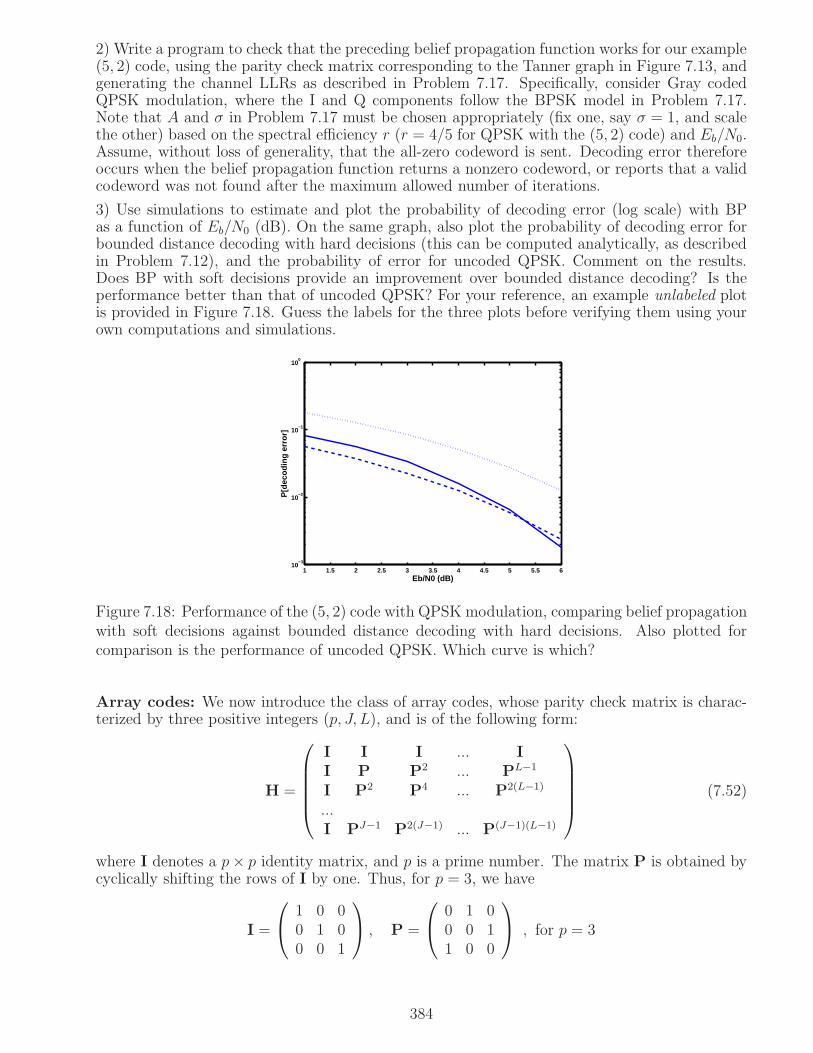
2) Write a program to check that the preceding belief propagation function works for our example(5, 2) code, using the parity check matrix corresponding to the Tanner graph in Figure 7.13, andgenerating the channel LLRs as described in Problem 7.17. Specifically, consider Gray codedQPSK modulation, where the I and Q components follow the BPSK model in Problem 7.17.Note that A and σ in Problem 7.17 must be chosen appropriately (fix one, say σ = 1, and scalethe other) based on the spectral efficiency r (r = 4/5 for QPSK with the (5, 2) code) and Eb/N0.Assume, without loss of generality, that the all-zero codeword is sent. Decoding error thereforeoccurs when the belief propagation function returns a nonzero codeword, or reports that a validcodeword was not found after the maximum allowed number of iterations.

3) Use simulations to estimate and plot the probability of decoding error (log scale) with BPas a function of Eb/N0 (dB). On the same graph, also plot the probability of decoding error forbounded distance decoding with hard decisions (this can be computed analytically, as describedin Problem 7.12), and the probability of error for uncoded QPSK. Comment on the results.Does BP with soft decisions provide an improvement over bounded distance decoding? Is theperformance better than that of uncoded QPSK? For your reference, an example unlabeled plotis provided in Figure 7.18. Guess the labels for the three plots before verifying them using yourown computations and simulations.

1 1.5 2 2.5 3 3.5 4 4.5 5 5.5 610

−3

10−2

10−1

100

Eb/N0 (dB)

P[d

ecod

ing

erro

r]

Figure 7.18: Performance of the (5, 2) code with QPSK modulation, comparing belief propagationwith soft decisions against bounded distance decoding with hard decisions. Also plotted forcomparison is the performance of uncoded QPSK. Which curve is which?

Array codes: We now introduce the class of array codes, whose parity check matrix is charac-terized by three positive integers (p, J, L), and is of the following form:

H =

I I I ... II P P2 ... PL−1

I P2 P4 ... P2(L−1)

...I PJ−1 P2(J−1) ... P(J−1)(L−1)

(7.52)

where I denotes a p× p identity matrix, and p is a prime number. The matrix P is obtained bycyclically shifting the rows of I by one. Thus, for p = 3, we have

I =

1 0 00 1 00 0 1

, P =

0 1 00 0 11 0 0

, for p = 3

384

The matrix P is a permutation matrix, in the sense that for any p× 1 vector u = (u1, ..., up)T ,

the vector Pu is a permutation of u. For this choice of P, the vector Pu = (up, u1, ..., up−1)T

is a cyclic shift of u by one. Raising P to an integer power k simply corresponds to applying ksuccessive cyclic shifts, so that Pk is a cyclic shift of the rows of I by k, and Pku is a cyclic shiftof u by k.

The parity check matrix H in (7.52) consists of JL p × p blocks, with the (j, l)th block beingP(j−1)(l−1), 1 ≤ j ≤ J , 1 ≤ l ≤ L. The code length n = pL, the number of columns (or variablenodes). The column weight equals J for each column (make sure you check this); that is, eachvariable node has degree J . The number of rows (or check nodes) equals pJ , but some of theserows may be redundant, so the dimension of the dual code n− k ≤ pJ . In fact, it can be shownthat exactly J − 1 rows are redundant. (To see why this might be true, add the first p rows, andthen the next p rows. What answers do you get? What does this tell you about the number oflinearly independent rows?) Thus, the rank of H equals n− k = pJ − (J − 1), so that the codedimension k = p(L− J) + J − 1. We therefore summarize as follows:

n = pL , k = p(L− J) + J − 1 for a (p, J, L) array code (7.53)

Popular choices of the variable node degree J = 3, 4. Analysis of code properties show that weshould restrict L ≤ p. We can, for example, use a large prime p and moderate sized L, or setL = p for a relatively small value of p.

4) Write a function to generate the parity check matrix of an array code, whose inputs are p, J, Land outputs are H, n, k.

function [H,n,k] = array_code(p,J,L)%Generates the parity check matrix for an array code%%INPUTS%p is a prime%J= check node degree (column weight), usually set to 3 or 4%L = parameter <= p that determines code length%%OUTPUTS%H = parity check matrix%%n = pL (code length)%%k = p(L-J)+J-1 (number of info bits)

%p times p identity matrixIblock = eye(p);% can use Matlab’s circshift operation on Iblock to generate P and its powers%for example, circshift(Iblock,[0 (j-1)*(l-1)]) generates the (j,l)th block of H%%NOW FILL IN THE FUNCTION!%%%

5) Consider an array code with p = 11, with L = p and J = 4, used as before with Gray codedQPSK and BICM. As before, use simulations to estimate and plot the probability of decodingerror (log scale) with BP as a function of Eb/N0 (dB) for a BICM system employing QPSK.Compare the performance (Eb/N0 for decoding error probability of 10−4) with the Shannonlimit for that spectral efficiency. To limit the simulation cost, you may wish to use a relativelysmall number of simulation runs to generate your plots, and to estimate the value of Eb/N0 theprobability of decoding error starts falling below, say, 10−2, and then use a larger number of runsfor a few carefully chosen values of Eb/N0 to see when the decoding error probability hits 10−4.How does this Eb/N0 compare with that required for 10−4 BER with uncoded QPSK?

6) Repeat 5) for larger values of the prime number p (still keeping L = p and J = 4), within thelimits of your computational infrastructure. For example, try p = 47.

385

7) Repeat 5) with large p and relatively small L; for example, p = 911 and L = 8, still keepingJ = 4. How does the code rate and spectral efficiency (with QPSK) compare with 5) and 6)?

Lab Report: Your lab report should answer the preceding questions in order, and should documentthe reasoning you used and the difficulties you encountered. Comment on the decoding errorprobability trends as you vary the code parameters.

386

Chapter 8

Dispersive Channels and MIMO

From the material in Chapters 4-6, we now have an understanding of commonly used modulationformats, noise models, and optimum demodulation for the AWGN channel model. Chapter 7discusses channel coding strategies for these idealized models. In this final chapter, we discussmore sophisticated channel models, and the corresponding signal processing schemes required atthe demodulator.

We first consider the following basic model for a dispersive channel: the transmitted signal passesthrough a linear time-invariant system, and is then corrupted by white Gaussian noise. The LTImodel is broadly applicable to wireline channels, including copper wires, cable and fiber opticcommunication (at least over shorter distances, over which fiber nonlinearities can be neglected),as well as to wireless channels with quasi-stationary transmitters and receivers. For wirelessmobile channels, the LTI model is a good approximation over durations that are small comparedto the time constants of mobility, but still fairly long on an electronic timescale (e.g., of the orderof milliseconds). Methods for compensating for the effects of a dispersive channel are genericallytermed equalization. We introduce two common design approaches for this purpose.

The first approach is singlecarrier modulation, which refers to the linear modulation schemesdiscussed in Chapter 4, where the symbol sequence modulates a transmit pulse occupying theentire available bandwidth. We discuss linear zero forcing (ZF) and Minimum Mean SquaredError (MMSE) equalization techniques, which are suboptimal from the point of view of mini-mizing error probability, but are intuitively appealing and less computationally complex thanoptimum equalization. (We refer the reader to more advanced texts for discussion of optimumequalization and its performance analysis.) We discuss adaptive implementation and geometricinterpretation for linear equalizers.

The second approach to channel dispersion is Orthogonal Frequency Division Multiplexing (OFDM),where linear modulation is applied in parallel to a number of subcarriers, each of which occupiesa bandwidth which is small compared to the overall bandwidth. OFDM may be viewed as amechanism for ISI avoidance. It is based on the observation that any complex exponential ej2πf0t

passes through any LTI system with transfer function H(f) unchanged except for multiplicationby H(f0). Thus, we can send a number of complex exponentials ej2πfit, termed subcarriers,in parallel through the channel, each multiplied by an information-bearing symbol, such thatinterference across subcarriers is avoided. The task of channel equalization therefore reduces tocompensating separately for the channel gains H(fi) for each such subcarrier. Parallelizing theproblem of equalization in this manner is particularly attractive when the underlying time domainimpulse response h(t) is complicated (e.g., an indoor wireless channel where there are a largenumber of paths with multiple bounces off walls and ceilings between transmitter and receiver).We discuss how this intuition is translated into practice using transceiver implementations usingdigital signal processing (DSP).

Finally, we discuss multiple antenna communication, also popularly known as Multiple Input

387

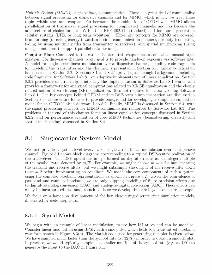
Multiple Output (MIMO), or space-time, communication. There is a great deal of commonalitybetween signal processing for dispersive channels and for MIMO, which is why we treat thesetopics within the same chapter. Furthermore, the combination of OFDM with MIMO allowsparallelization of transceiver signal processing for complicated channels, and has become thearchitecture of choice for both WiFi (the IEEE 802.11n standard) and for fourth generationcellular systems (LTE, or long term evolution). Three key concepts for MIMO are covered:beamforming (directing energy towards a desired communication partner), diversity (combatingfading by using multiple paths from transmitter to receiver), and spatial multiplexing (usingmultiple antennas to support parallel data streams).

Chapter Plan: Compared to the earlier chapters, this chapter has a somewhat unusual orga-nization. For dispersive channels, a key goal is to provide hands-on exposure via software labs.A model for singlecarrier linear modulation over a dispersive channel, including code fragmentsfor modeling the transmitter and the channel, is presented in Section 8.1. Linear equalizationis discussed in Section 8.2. Sections 8.1 and 8.2.1 provide just enough background, includingcode fragments, for Software Lab 8.1 on adaptive implementation of linear equalization. Section8.2.2 provides geometric insight into why the implementation in Software Lab 8.1 works, andprovides a framework for analytical computations related to MMSE equalization and the closelyrelated notion of zero-forcing (ZF) equalization. It is not required for actually doing SoftwareLab 8.1. The key concepts behind OFDM and its DSP-centric implementation are discussed inSection 8.3, whose entire focus is to provide background for developing a simplified simulationmodel for an OFDM link in Software Lab 8.2. Finally, MIMO is discussed in Section 8.4, withthe signal processing concepts for MIMO communication reinforced by Software Lab 8.3. Theproblems at the end of this chapter focus on linear equalization concepts discussed in Section8.2.2, and on performance evaluation of core MIMO techniques (beamsteering, diversity andspatial multiplexing) discussed in Section 8.4.

8.1 Singlecarrier System Model

We first provide a system-level overview of singlecarrier linear modulation over a dispersivechannel. Figure 8.1 shows block diagrams corresponding to a typical DSP-centric realization ofthe transceiver. The DSP operations are performed on digital streams at an integer multipleof the symbol rate, denoted by m/T . For example, we might choose m = 4 for implementingthe transmit and receive filters, but we might subsample the output of the receive filter downto m = 2 before implementing an equalizer. We model the core components of such a systemusing the complex baseband representation, as shown in Figure 8.2. Given the equivalence ofpassband and complex baseband, we are only skipping modeling of finite precision effects dueto digital-to-analog conversion (DAC) and analog-to-digital conversion (ADC). These effects caneasily be incorporated into models such as those we develop, but are beyond our current scope.

We focus on a hands-on development of the key ideas using discrete time simulation models,illustrated by code fragments.

8.1.1 Signal Model

We begin with an example of linear modulation, to see how ISI arises and can be modeled.Consider linear modulation using BPSK with a sine pulse, which leads to a transmitted basebandwaveform shown in Figure 8.3(a). The Matlab code used for generating this plot is given below.We have sampled much faster than the symbol rate (at 32/T ) in order to obtain a smooth plot.In practice, we would typically sample at a smaller multiple of the symbol rate (e.g. at 4/T ) togenerate the input to the DAC in Figure 8.1.

388

I

Q Q

ADC

ADC

DSP for

receiver

functions

QDAC

DACI

Q

PassbandChannel

(synchronization,equalization,demodulation)

at rate m/T)(implemented

filterTransmit

Symbols

rate 1/T

filter

at rate m/T)(implemented

Receive

(includes coarse analogpassband filtering)

waveformsbasebandAnalog

Up

converter

Down

converter

Estimated

symbols

I

I

rate m/TstreamsDigital

Figure 8.1: Typical DSP-centric transceiver realization. Our model does not include the blocksshown in dashed lines. Finite precision effects due to digital to analog conversion (DAC) andanalog to digital conversion (ADC) are not considered. The upconversion and downconversionoperations are not modeled. The passband channel is modeled as an LTI system in complexbaseband.

Estimated

TX

Transmit

Filter

Cg (t)

ChannelFilter

g (t)RX

ReceiveFilterb[n]

Noise

Rate 1/T

Sampler,rate m/T

ProcessingSignal

Receiver

(Synchronization,Equalization,Demodulation)

Symbols

symbolsg (t)

Figure 8.2: Block diagram of a linearly modulated system, modeled in complex baseband.

389

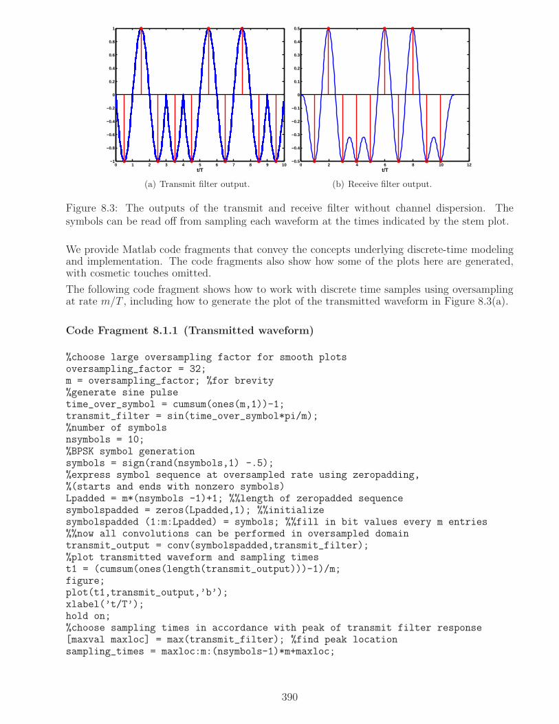
0 1 2 3 4 5 6 7 8 9 10−1

−0.8

−0.6

−0.4

−0.2

0

0.2

0.4

0.6

0.8

1

t/T

(a) Transmit filter output.

0 2 4 6 8 10 12−0.5

−0.4

−0.3

−0.2

−0.1

0

0.1

0.2

0.3

0.4

0.5

t/T

(b) Receive filter output.

Figure 8.3: The outputs of the transmit and receive filter without channel dispersion. Thesymbols can be read off from sampling each waveform at the times indicated by the stem plot.

We provide Matlab code fragments that convey the concepts underlying discrete-time modelingand implementation. The code fragments also show how some of the plots here are generated,with cosmetic touches omitted.

The following code fragment shows how to work with discrete time samples using oversamplingat rate m/T , including how to generate the plot of the transmitted waveform in Figure 8.3(a).

Code Fragment 8.1.1 (Transmitted waveform)

%choose large oversampling factor for smooth plotsoversampling_factor = 32;m = oversampling_factor; %for brevity%generate sine pulsetime_over_symbol = cumsum(ones(m,1))-1;transmit_filter = sin(time_over_symbol*pi/m);%number of symbolsnsymbols = 10;%BPSK symbol generationsymbols = sign(rand(nsymbols,1) -.5);%express symbol sequence at oversampled rate using zeropadding,%(starts and ends with nonzero symbols)Lpadded = m*(nsymbols -1)+1; %%length of zeropadded sequencesymbolspadded = zeros(Lpadded,1); %%initializesymbolspadded (1:m:Lpadded) = symbols; %%fill in bit values every m entries%%now all convolutions can be performed in oversampled domaintransmit_output = conv(symbolspadded,transmit_filter);%plot transmitted waveform and sampling timest1 = (cumsum(ones(length(transmit_output)))-1)/m;figure;plot(t1,transmit_output,’b’);xlabel(’t/T’);hold on;%choose sampling times in accordance with peak of transmit filter response[maxval maxloc] = max(transmit_filter); %find peak locationsampling_times = maxloc:m:(nsymbols-1)*m+maxloc;

390

sampled_outputs = transmit_output(sampling_times);stem((sampling_times-1)/m,sampled_outputs,’r’)hold off;

If this waveform now goes through an ideal channel, and we use a receive filter with impulseresponse matched to the transmitted pulse, then the waveform we obtain is shown in Figure8.3(b). The transmit filter impulse response is time limited to length T and hence square rootNyquist (see Chapter 4), hence the net response to a single symbol, which is a cascade of thetransmit filter with its matched filter, is Nyquist. It follows that, by sampling at the rightmoments (as marked on the plot), we can recover the symbols exactly.

We now provide a code fragment to model the channel and receive filter; it can be employed formodeling both ideal and dispersive channels. Appending it to code fragment 8.1.1 generates andplots the noiseless received waveform.

Code Fragment 8.1.2 (Modeling the channel and receive filter)

dispersive = 0; %set this to 0 for ideal channel, and to 1 for dispersive channelif dispersive == 0,channel = 1;elsechannel = [0.8;zeros(m/2,1);-0.7;zeros(m,1);-0.6];%(or substitute your favorite choice of dispersive channel)end%noiseless receiver inputreceive_input = conv(transmit_output,channel);t2 = (cumsum(ones(length(receive_input)))-1)/m;figure;plot(t2,receive_input);xlabel(’t/T’);%receive filter matched to transmit filter%(would also need to conjugate if complex-valued)receive_filter = flipud(transmit_filter);%receive filter output (normalized to account for oversampling)receive_output = (1/m)*conv(receive_input,receive_filter);t3 = (cumsum(ones(length(receive_output),1))-1)/m;%plot receive filter output together with sample locations chosen based on peak of net responsefigure;plot(t3,receive_output,’b’);xlabel(’t/T’);hold on;%effective pulse at channel outputpulse = conv(transmit_filter,channel);%effective pulse at receive filter output (normalized to account for oversampling)rx_pulse = conv(pulse,receive_filter)/m;[maxval maxloc] = max(rx_pulse);rx_sampling_times = maxloc:m:(nsymbols-1)*m+maxloc;rx_sampled_outputs = receive_output(rx_sampling_times);stem((rx_sampling_times-1)/m,rx_sampled_outputs,’r’);hold off;

Figure 8.4 shows a dispersive channel and the corresponding noiseless receive filter output. Theeffective pulse given by the cascade of the transmit, channel and receive filters is no longer

391

−0.5 0 0.5 1 1.5 2−0.8

−0.6

−0.4

−0.2

0

0.2

0.4

0.6

0.8

t/T

(a) Dispersive channel.

0 2 4 6 8 10 12 14−0.4

−0.2

0

0.2

0.4

0.6

0.8

1

t/T

(b) Receive filter output.

Figure 8.4: When the transmitted waveform passes through the dispersive channel shown, wecan no longer read off the symbols reliably by sampling the output of the receive filter. For thisparticular set of symbols, one of the symbols is estimated incorrectly, even though there is nonoise.

Nyquist, hence we do not expect a symbol decision based on a single sample to be reliable.Figure 8.4(b) shows the severe distortion due to ISI with a “best effort” choice of sampling times(chosen based on the peak of the effective pulse). In particular, for the specific symbol sequenceshown, one (out of ten) of the symbol estimates obtained by taking the signs of these samples isincorrect.

0 0.2 0.4 0.6 0.8 1 1.2 1.4 1.6 1.8 2−20

−15

−10

−5

0

5

10

15

20

t/T

(a) Ideal channel.

0 0.2 0.4 0.6 0.8 1 1.2 1.4 1.6 1.8 2−30

−20

−10

0

10

20

30

t/T

(b) Dispersive channel.

Figure 8.5: Eye diagrams with and without channel dispersion. The eye is closed for the channelconsidered, which means that reliable symbol decisions are not possible without equalization.

Eye diagrams: A classical technique for visualizing the effect of ISI is the eye diagram. Itis constructed by overlapping multiple segments of the received waveform over a fixed window,which tells us how different combinations of symbols could potentially create ISI. For an idealchannel and square root Nyquist pulses at either end, the eye is open, as shown in Figure 8.5(a).However, for the dispersive channel in Figure 8.4(b), we see from Figure 8.5(b) is closed. An openeye implies that, by an appropriate choice of sampling times, we can make reliable single-samplesymbol decisions, while a closed eye means that more sophisticated equalization techniques areneeded for symbol recovery.

Physically, an eye diagram can be generated using an oscilloscope with the baseband modulated

392

signal as the vertical input, with horizontal sweep triggered at the symbol rate. A code fragmentfor generating the eye pattern from discrete time samples at rate m/T is given below. (WhileMatlab has its own eye diagram routine, this code fragment is provided in order to clearly conveythe concept.) The output of the receive filter generated in code fragment 8.1.2 is the input tothis fragment, but in general, we could plot an eye diagram based on the baseband waveform atany stage in the system. For complex baseband signals, we would plot the eye diagrams for theI and Q components separately.

Code Fragment 8.1.3 (Eye diagram)

%remove edge effects before doing eye diagramr1 = receive_out(m/2:m/2+nsymbols*m-1);%horizontal display length in number of symbol intervalsK=2;%break into non-overlapping tracesR1=reshape(r1,K*m,length(r1)/(K*m));%now enforce continuity across traces%(append to each trace the first element of the next trace)row1 = R1(1,:);L=length(row1);row_pruned = row1(2:L);R_pruned = R1(:,1:L-1);R2 = [R_pruned;row_pruned];time = (0:K*m)/m; %time as a multiple of symbol intervalplot(time,R2);xlabel(’t/T’);

8.1.2 Noise Model and SNR

In continuous time, our model for the noisy input to the receive filter is

y(t) =∑

n

b[n]p(t− nT ) + n(t) (8.1)

where p(t) = (gTX ∗ gC)(t) is the “effective pulse” given by the cascade of the transmit pulseand the channel filter, b[n] is the symbol sequence, which is in general complex-valued, andn(t) is complex WGN with PSD σ2 = N0

2. We translate this model directly into discrete time

by constraining t = kT/m + τ , where m/T is the sampling rate (m a positive integer) and τequals the sampling offset. The noise at the input to the receive filter is now modeled as discretetime white Gaussian noise (WGN) with variance σ2 = N0

2per dimension. As we well know from

Chapter 6, the absolute value of the noise variance is meaningless unless we also specify the signalscaling, hence we fix either the signal or noise strength, and set the other based on SNR measuressuch as Eb/N0 or Es/N0. Here Es = E[|b[n]|2]||p||2 for the model (8.1), and Eb = Es/ log2Mas usual, where M is the constellation size. Inner products and norms are computed in discretetime.

Note that, with the preceding convention, the noise energy in a fixed time interval scales up withthe sampling rate, and so does the signal energy (since we have more samples whose energieswe are adding up), with the SNR converging to the continuous-time SNR as the sampling rategets large. However, for a sampling rate that is a small multiple of the symbol rate, the SNR forthe discrete time system can, in general, be different from that in the original continuous timesystem. We do not worry about this distinction here. The following code fragment illustratesadding noise to our simulation model.

393

We now provide a code fragment which adds discrete time WGN to the receive filter input,resulting in colored noise at the output. We add this to the signal component already computedin code fragment 8.1.2.

Code Fragment 8.1.4 (Noise modeling)

bn_energy = 1;% for BPSK with current normalizationEs = bn_energy*(pulse’*pulse); %pulse is cascade of transmit and channel filtersconstellation_size=2; %for BPSKEb = Es/log2(constellation_size);%specify Eb/N0 in dBebnodb=5;ebnoraw = 10^(ebnodb/10); %raw Eb/N0N0=Eb/ebnoraw;%noise standard deviation per dimensionsigma = sqrt(N0/2);%noise at input to receive filter%(would also need to add an imaginary component for complex-valued signals)noise_receive_input = sigma*randn(size(receive_input));%(would also need to add an imaginary component for complex-valued signals)%noise_receive_input = noise_receive_input + 1i*sigma*randn(size(receive_input));%noise at output of receive filternoise_receive_output = (1/m)*conv(noise_receive_input,receive_filter);%noisy receive filter outputreceive_output_noisy = receive_output + noise_receive_output;

8.2 Linear equalization

We have seen that single-sample symbol decisions are unreliable when the eye is closed. However,what if we are willing to use multiple samples for each symbol decision? Typically, the transmitterand receiver may implement fixed filters in DSP at a faster sampling rate than the sampling rateused eventually for equalization. Thus, suppose that we have samples at rate m/T from theoutput of the receive filter, but we now wish to use rate q/T samples for equalization, whereq divides m. For example, we may have m = 4 and q = 2. We subsample the output of thereceive filter, taking one out of every m/q samples, and then use L consecutive samples, collectedinto a vector r[n], to make a decision on symbol b[n]. We would want to choose these samplesso that the bulk of the response due to b[n] falls within the observation interval over whichwe collect these samples. When we want to make a decision on the next symbol b[n + 1], wemust slide this observation interval over by T in order to obtain the received vector r[n + 1].Since our sampling rate is now q/T , this corresponds to an offset of q samples between successiveobservation intervals. Note that an observation interval typically spans multiple symbol intervals,so that successive observation intervals overlap Figures 8.6 and 8.7 illustrate this concept for achannel of length L = 4 obtained by sampling at rate 2/T , so that q = 2. The overlap betweensuccessive observation intervals equals L− q = 2 samples.

The transmit, channel and receive filters are LTI systems and the noise is stationary, and succes-sive symbols are input to the system spaced by time T . Since the discrete time symbol sequenceis stationary as well, the statistics of the signal at any stage of the system are invariant to shiftsby integer multiples of T . Such periodicity in the statistics is termed cyclostationarity. Thisimplies that the statistics of the noise and ISI seen in different observation intervals are identical:the only change is in which symbol plays the role of desired symbol. In particular, comparing

394

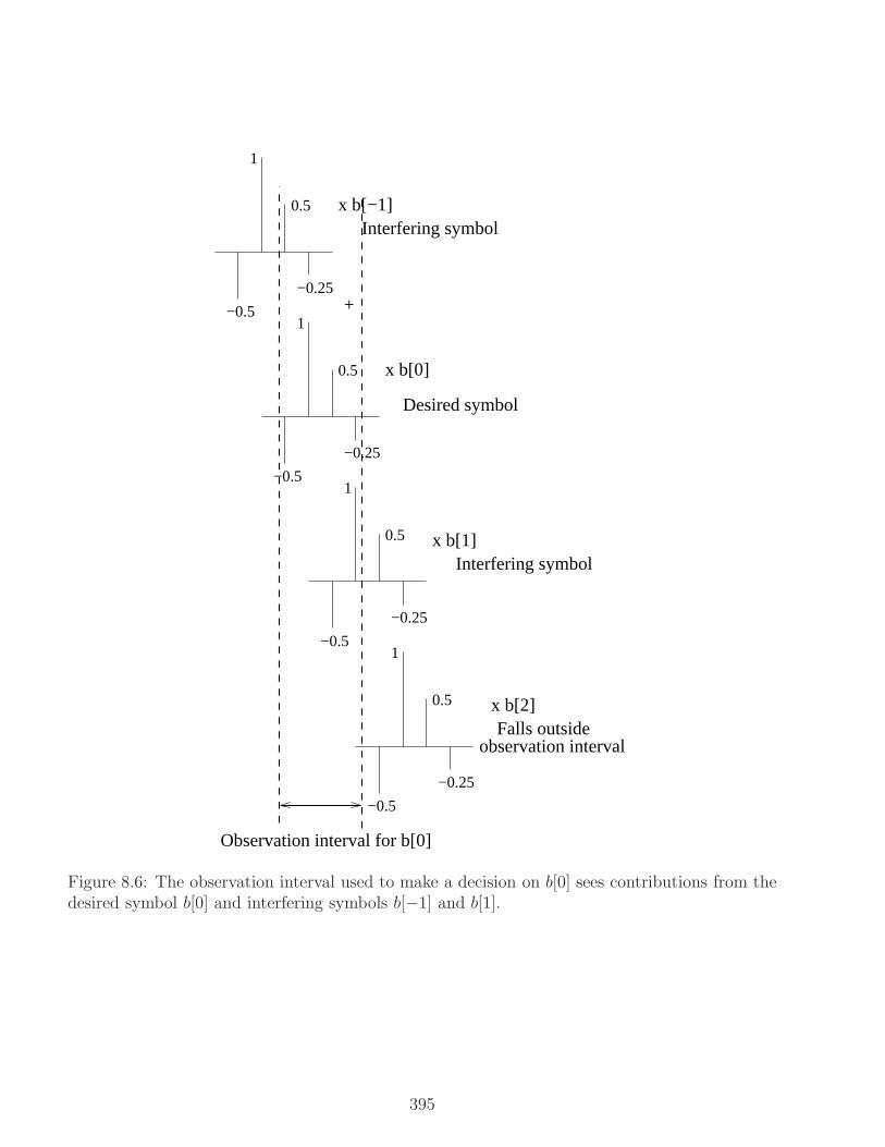
observation interval

1

0.5

−0.25

−0.5

1

0.5

−0.25

−0.5

1

0.5

−0.25

−0.5

1

0.5

−0.25

−0.5

x b[−1]

x b[0]

x b[1]

x b[2]

+

Observation interval for b[0]

Desired symbol

Interfering symbol

Interfering symbol

Falls outside

Figure 8.6: The observation interval used to make a decision on b[0] sees contributions from thedesired symbol b[0] and interfering symbols b[−1] and b[1].

395

Observation interval for b[1]

1

0.5

−0.25

−0.5

1

0.5

−0.25

−0.5

1

0.5

−0.25

−0.5

1

0.5

−0.25

−0.5

x b[−1]

x b[0]

x b[1]

x b[2]

+

Desired symbol

Interfering symbol

Falls outsideobservation interval

Interfering symbol

Figure 8.7: The observation interval used to make a decision on b[1] sees contributions from thedesired symbol b[1] and interfering symbols b[0] and b[2]. Comparing with Figure 8.6, the rolesof the symbols has shifted by one.

396

Figures 8.6 and 8.7, we see that the roles of desired and interfering symbols shifts by one as we gofrom the observation interval for b[0] to that for b[1]. Thus, an appropriately designed strategyfor handling ISI over a given observation interval should work for other observation intervals aswell. This opens up the possibility of realizing adaptive equalizers which can learn enough aboutthe statistics of the ISI and noise to compensate for them.

We focus here on linear equalization, which corresponds to using the decision statistic cT r[n] toestimate b[n], where c is an appropriately chosen correlator. The choice of c can be independentof n, by virtue of cyclostationarity. For BPSK signaling, for example, this leads to a decisionrule

b[n] = sign(

cTr[n])

(8.2)

8.2.1 Adaptive MMSE Equalization

While constraining ourselves to linear equalization is suboptimal (discussion of optimal equaliza-tion is beyond our present scope), we can try to optimize c to combat ISI and noise. In particular,the linear MMSE criterion corresponds to choosing c so as to minimize the mean squared error(MSE) between the decision statistic and the desired symbol, defined as

MSE = J(c) = E[

(cT r[n]− b[n])2]

(8.3)

Minimizing the MSE in this fashion leads to minimizing the contribution due to ISI and noiseat the correlator output, which is clearly a desirable outcome.

The MSE is a quadratic function of c, and can therefore be minimized by setting its gradientwith respect to c to zero. Due to linearity, the gradient can be taken inside the expectation, andwe obtain

∇cJ(c) = 2E[

r[n](cT r[n]− b[n])]

= 2E[

r[n](rT [n]c− b[n])]

DefiningR = E

[

r[n]rT [n]]

, p = E [b[n]r[n]] (8.4)

we can rewrite the gradient of the MSE as

∇cJ(c) = 2 (Rc− p) (8.5)

Setting the gradient to zero yields the following expression for the MMSE correlator:

cMMSE = R−1p (8.6)

In order to compute this, we must know, or be able to estimate, the expectations in (8.4). If weknow the transmit filter, the channel filter, the receive filter, the sampling times, and the noisePSD, we can compute these expectations using a model such as (8.13). However, we often donot have explicit knowledge of one or more of these quantities. Thus, an attractive approach inpractice is to exploit the stationarity of the model as we vary n to estimate expectations usingtheir empirical averages. These expectations involve the received vectors r[n], which we of coursehave access to, and the symbols b[n], which we assume we have access to over a training period inwhich a known sequence of symbols is transmitted. This approach leads to adaptive equalizationtechniques that do not require explicit knowledge or estimates of the model parameters.

Least Squares Adaptation: Assuming that the first ntraining symbols are known, leastsquares adaptation corresponds to replacing the expectations in (8.4) by their empirical averagesas follows:

R =1

ntraining

ntraining∑

n=1

r[n]rT [n] , p =1

ntraining

ntraining∑

n=1

b[n]r[n] (8.7)

397

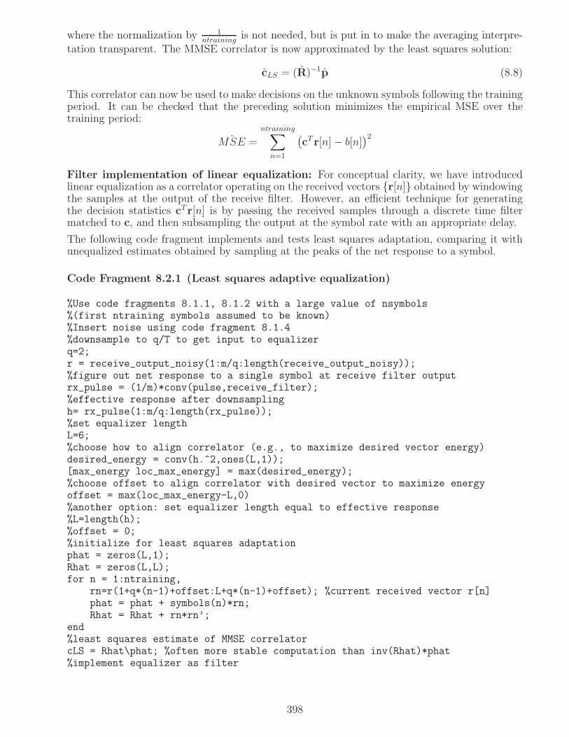
where the normalization by 1ntraining

is not needed, but is put in to make the averaging interpre-tation transparent. The MMSE correlator is now approximated by the least squares solution:

cLS = (R)−1p (8.8)

This correlator can now be used to make decisions on the unknown symbols following the trainingperiod. It can be checked that the preceding solution minimizes the empirical MSE over thetraining period:

ˆMSE =

ntraining∑

n=1

(

cT r[n]− b[n])2

Filter implementation of linear equalization: For conceptual clarity, we have introducedlinear equalization as a correlator operating on the received vectors r[n] obtained by windowingthe samples at the output of the receive filter. However, an efficient technique for generatingthe decision statistics cT r[n] is by passing the received samples through a discrete time filtermatched to c, and then subsampling the output at the symbol rate with an appropriate delay.

The following code fragment implements and tests least squares adaptation, comparing it withunequalized estimates obtained by sampling at the peaks of the net response to a symbol.

Code Fragment 8.2.1 (Least squares adaptive equalization)

%Use code fragments 8.1.1, 8.1.2 with a large value of nsymbols%(first ntraining symbols assumed to be known)%Insert noise using code fragment 8.1.4%downsample to q/T to get input to equalizerq=2;r = receive_output_noisy(1:m/q:length(receive_output_noisy));%figure out net response to a single symbol at receive filter outputrx_pulse = (1/m)*conv(pulse,receive_filter);%effective response after downsamplingh= rx_pulse(1:m/q:length(rx_pulse));%set equalizer lengthL=6;%choose how to align correlator (e.g., to maximize desired vector energy)desired_energy = conv(h.^2,ones(L,1));[max_energy loc_max_energy] = max(desired_energy);%choose offset to align correlator with desired vector to maximize energyoffset = max(loc_max_energy-L,0)%another option: set equalizer length equal to effective response%L=length(h);%offset = 0;%initialize for least squares adaptationphat = zeros(L,1);Rhat = zeros(L,L);for n = 1:ntraining,

rn=r(1+q*(n-1)+offset:L+q*(n-1)+offset); %current received vector r[n]phat = phat + symbols(n)*rn;Rhat = Rhat + rn*rn’;

end%least squares estimate of MMSE correlatorcLS = Rhat\phat; %often more stable computation than inv(Rhat)*phat%implement equalizer as filter

398

h_equalizer = flipud(cLS); %would also need conjugation for complex signalsequalizer_output = conv(r,h_equalizer);%sample filter output at symbol rate after appropriate delaydelay = length(h_equalizer)+offset;%symbol decision statisticsdecision_stats = equalizer_output(delay:q:delay+(nsymbols-1)*q);%payload = non-training symbolspayload = symbols(ntraining+1:nsymbols);%estimate of payload (for BPSK)payload_estimate = sign(decision_stats(ntraining+1:nsymbols));%number of errorsnerrors = sum(ne(payload,payload_estimate))%COMPARE WITH UNEQUALIZED ESTIMATES%unequalized estimates obtained by sampling at peaks of effective response[maxval maxloc] = max(h);sampling_times = maxloc:q:(nsymbols-1)*q+maxloc;unequalized_decision_stats = r(sampling_times);sampled_outputs = transmit_output(sampling_times);%estimate of payload (for BPSK)payload_estimate_unequalized = sign(unequalized_decision_stats(ntraining+1:nsymbols));%number of errorsnerrors_unequalized = sum(ne(payload,payload_estimate_unequalized))

Putting code fragments 8.1.1, 8.1.2, 8.1.4 and 8.2.1 together, we obtain a simulation model foradaptive linear equalization over a dispersive channel. As a quick example, for the dispersivechannel considered, at Eb/N0 of 7 dB, we estimate (using nsymbols = 10000, ntraining = 100)the error probability after equalization at rate 2/T (q = 2) to be about 3.5 × 10−3 and theunequalized error probability to be about 0.16. Linear equalization is quite effective in this case,although it exhibits some degradation relative to the ideal BPSK error probability of 7.7× 10−4.We can now build on this code base to run a variety of experiments, as suggested in SoftwareLab 8.1: for example, probability of error as a function of Eb/N0 for different equalizer lengths,for different channel models, and for different choices of the transmit and receive filters. Ourmodel extends easily to complex-valued constellations, as discussed below.

Extension to complex-valued signals: All of the preceding development goes through forcomplex-valued constellations and signals, except that vector transposes xT are replaced byconjugate transposes xH . Indeed, the Matlab code fragments we provide here already includethis level of generality, since we use the conjugate transpose operation x′ when computing thetranspose for real-valued x. All that is needed to employ these code fragments is to make thesymbols complex-valued, and to add an imaginary component to the noise model in code fragment8.1.4. We skip derivations, and state that the decision statistics are given by cHr[n], the MSEexpression is

MSE = J(c) = E[

|cHr[n]− b[n]|2]

and the MMSE solution is given by (8.6) as before, with

R = E[

r[n]rH [n]]

, p = E [b∗[n]r[n]] (8.9)

As before, these statistical expectations can be replaced by empirical averages for a least squaresimplementation.

We now have the background required for a hands-on exposure to equalization through SoftwareLab 8.1.

399

8.2.2 Geometric Interpretation and Analytical Computations

Computer simulations using the code fragments in Sections 8.1 and 8.2 show that adaptiveMMSE equalization works well, at least in the specific examples considered in these sections,and in Software Lab 8.1. We now develop geometric insight into why linear equalization workswell when it does, and when it might run into trouble. We stick with real-valued signals, but theresults extend easily to complex-valued signals, as noted in the appropriate places. This sectionis not required for doing Software Lab 8.1.

Consider the example depicted in Figures 8.6 and 8.7, where the overall sampled response (atrate 2/T ) to a single symbol is assumed to be

h = (..., 0,−0.5, 1, 0.5,−0.25, 0, ...)

Consider an observation interval (i.e., equalizer length) of length L = 4, aligned with the responseto the desired symbol as depicted in Figures 8.6 and 8.7. As shown in code fragment 8.2.1, wecan also choose smaller or larger observation intervals, and optimize their alignment using somecriterion (in the code fragment, the criterion is maximizing the energy of the desired responsefalling into the observation interval). In addition to the contribution to r[n] due to b[n], we alsohave contributions from other symbols before and after it in the sequence, corresponding to partsof appropriately shifted versions of the response h. For example, the response to b[n+ 1] fallingin the nth observation interval is obtained by shifting h by q = 2 and then windowing. Thereceived vector r[n] can therefore be written as follows.

Model for L = 4: Two interfering symbols fall into the observation interval. The observationinterval is large enough to accommodate the entire response due to the desired symbol.

r[n] = b[n]

−0.510.5

−0.25

+ b[n + 1]

00

−0.51

+ b[n− 1]

0.5−0.25

00

+w[n] (8.10)

where our convention is that time progresses downward, and where w[n] denotes noise. Thevector multiplying b[n] is the desired vector, while the others are interference vectors. Figure 8.6corresponds to n = 0, while Figure 8.7 corresponds to n = 1.

In order to obtain the preceding model, the vector corresponding to a given symbol is obtainedby appropriately shifting h, and then windowing to the observation interval. In order to ensurethat the modeling approach is clear, we also provide the model for L = 3, where the observationinterval is lined up with the first three elements of the response to the desired symbol, and L = 6,where the observation interval contains two additional samples on either side of the response tothe desired symbol.

Model for L = 3: The observation interval is smaller than the desired symbol response. Twointerfering symbols fall in the interval.

r[n] = b[n]

−0.510.5

+ b[n + 1]

00

−0.5

+ b[n− 1]

0.5−0.25

0

+w[n] (8.11)

Model for L = 6: The observation interval is larger than the desired symbol response. Four

400

interfering symbols fall in the interval.

r[n] = b[n]

0−0.510.5

−0.250

+ b[n + 1]

000

−0.510.5

+ b[n + 2]

0000

−0.5

+ b[n− 1]

10.5

−0.25000

+ b[n− 2]

−0.2500000

+w[n]

(8.12)

Vector model for ISI: In general, we can write the received vector over observation interval nas follows:

r[n] = b[n]u0 +∑

k 6=0

b[n + k]uk +w[n] (8.13)

where b[n], u0 are the desired symbol and vector, respectively; b[n + k], uk for k 6= 0 areinterference symbols and vectors, respectively; and w[n] ∼ N(0,Cw) denotes the vector of noisesamples at the output of the receive filter, windowed to the current observation interval. Foran equalizer working with rate q/T samples, we have already noted that successive observationintervals are offset by q samples. Clearly, the structure of the ISI remains the same as we go fromobservation interval n to n + 1, but the roles of the symbols are shifted by one: for the n + 1stobservation interval, b[n + 1] is the desired symbol multiplying u0, while b[n + 1 + k] for k 6= 0is the interfering symbol multiplying uk.

Modeling the output of a linear correlator: A linear correlator c operating on the receivedvector produces the following output:

cT r[n] = b[n]cTu0 +∑

k 6=0

b[n + k]cTuk + cTw[n] (8.14)

where the first term is the desired term, the second term is the ISI at the correlator output,and the third term is the noise at the correlator output. While the ultimate performance metricof interest is the error probability, a convenient metric that is easy to compute is the signal-to-interference-plus-noise ratio (SINR) at the output of the linear correlator, defined as the ratio ofthe average energy of the desired term, to those of the undesired terms:

SINR =E[

|b[n]cTu0|2]

E

[

|∑k 6=0 b[n + k]cTuk + cTw[n]|2] (8.15)

Assuming that the symbols are uncorrelated with E[|b[n]|2] ≡ σ2b and are independent of the

noise, we obtain the following expression for the SINR:

SINR =σ2b |cTu0|2

σ2b

∑

k 6=0 |cTuk|2 + cTCwc(8.16)

Choosing c to minimize the MSE (8.3) means that we would like to have cT r[n] ≈ b[n]. Thismeans that, if the linear MMSE equalizer is working, then cTu0 ≈ 1, and the ISI terms cTuk,

401

k 6= 0, and the output noise variance cTCwc, are small. The MMSE criterion represents atradeoff between ISI and noise at the output. To see why, let us consider the closely relatedcriterion of zero-forcing equalization. While the noise in the example considered in our codefragments is colored, let us first consider white noise for simplicity: w[n] ∼ N(0, σ2I), so thatthe output noise cTw[n] ∼ N(0, σ2||c||2).

Desired vector0

u1

u−1

u0PI

...

Interference subspace

u

Figure 8.8: The zero-forcing correlator projects the received signal along P⊥I u0, the projection

of the desired signal vector orthogonal to the interference subspace.

The geometry of zero-forcing equalization: The zero-forcing (ZF) equalizer is a linearequalizer chosen to set the ISI terms at the output exactly to zero:

cTuk = 0 , k 6= 0 (8.17)

while scaling the desired term to the right level:

cTu0 = 1 (8.18)

The first condition (8.17) means that c must be orthogonal to the interference subspace, which isour term for the subspace spanned by the interference vectors uk, k 6= 0. If (8.17) is satisfied,then the second condition (8.18) can only be satisfied if the desired vector u0 does not lie in theinterference subspace, otherwise we would have cTu0 = 0 (why?). Thus, the zero-forcing equalizerexists only if the desired vector u0 is linearly independent of the interference vectors uk, k 6= 0,in which case it has a nonzero component P⊥

I u0 orthogonal to the interference subspace, as shownin Figure 8.8. In this case, if we choose c to be a scalar multiple of this orthogonal component,then (8.17) is satisfied by construction. and (8.18) can be satisfied by choosing the scale factorappropriately, as discussed shortly. And indeed, while the solution to (8.17) and (8.18) need notbe unique, it can be shown (see Problem 8.5) that choosing cZF = αP⊥

I u0 is optimal (in terms ofminimizing error probability or maximizing SNR) among all possible ZF solutions, assuming thatthe noise vector w[n] is white Gaussian. As we shall see, the performance of the ZF correlatordepends on the length of this orthogonal projection P⊥

I u0 relative to that of the desired signal

vector u0: the smaller this relative length||P⊥

I u0||||u0|| , the poorer the performance.

For the model (8.10) for an equalizer of length L = 4, the signal vectors live in a space ofdimension 4, with 2 interference vectors. It is quite clear that the desired vector is indeedlinearly independent of the interference vectors, and we expect the ZF correlator to exist. For

402

the model (8.10) for L = 3, we again have 2 interference vectors, and it again appears thatthe ZF correlator should exist, although we would expect the performance to be poorer becausethe relative length of the orthogonal projection can be expected to be smaller. Of course, suchintuition must be quantified by explicit computation of the ZF correlator and its performance,which we discuss next.

Computation of the ZF correlator: Let us now obtain an explicit expression for the ZFcorrelator given the vector ISI model (8.13). Suppose that the signal vectors uk are written ascolumns in a matrix U as follows:

U = [...u−1u0u1...] (8.19)

The ZF conditions (8.17)-(8.18) can be compactly written as

UTcZF = e (8.20)

where e = (...0, 1, 0, ...)T is a unit vector with one corresponding to the column u0 and zeros cor-responding to columns uk, k 6= 0. Further, we can write the ZF correlator as a linear combinationof the signal vectors (any component orthogonal to all of the uk can only add noise):

cZF = Ua (8.21)

Plugging into (8.20), we obtainUTUa = e

so thata =

(

UTU)−1

e

assuming invertibility, which in turn requires that the signal vectors uk are linearly independent(see Problem 8.6). Substituting into (8.21), we obtain that

cZF = U(

UTU)−1

e , ZF correlator for white noise (8.22)

Noise enhancement: By “looking” along the direction of the orthogonal component P⊥I u0

shown in Figure 8.8, the ZF equalizer nulls out the interference vectors. When we plug in (8.17)-(8.18), the output SINR expression in (8.16) reduces to the output SNR. Setting Cw = σ2I, weobtain

SNRZF =σ2b

σ2||cZF ||2, ZF SNR for white noise (8.23)

On the other hand, if we ignore ISI, then we know from Chapter 6 that the optimal correlator inAWGN is a scalar multiple of the desired vector u0. Relative to this “matched filter” solution, theZF correlator incurs loss in SNR, termed noise enhancement. The reason that we say the noiseis getting enhanced (as opposed to the signal getting reduced) is that, if we scale the correlatorto keep the desired contribution at the output constant as in (8.18), then the degradation inSNR corresponds to an increase in the noise variance. For an ideal system with no ISI, thereceived vector is given by r[n] = b[n]u0 +w[n]. Setting c = u0, we have cT r[n] = b[n]||u0||2 +N(0, σ2||u0||2), from which it is easy to see that the output SNR is given by

SNRMF =E[|b[n]|2]||u0||2

σ2=σ2b ||u0||2σ2

, matched filter bound for white noise (8.24)

This is termed the matched filter (MF) bound on SNR, and is an unrealizable (because we haveignored ISI) benchmark that we can compare the performance of linear equalization strategiesagainst. In particular, the noise enhancement ζ can be defined as the ratio by which the ZF SNRis smaller than the MF benchmark:

ζ =SNRMF

SNRZF= ||u0||2||cZF ||2 , noise enhancement for white noise (8.25)

403

Let us first interpret this geometrically. Setting cZF = αP⊥I u0, the condition (8.18) corresponds

to1 = 〈cZF ,u0〉 = α〈P⊥

I u0,u0〉 = α||P⊥I u0||2 (8.26)

The last equality follows because u0 decomposes into its projection onto the interference sub-space PIu0 and its orthogonal projection P⊥

I u0. Since these two components are orthogonal bydefinition, we have

〈P⊥I u0,u0〉 = 〈P⊥

I u0,PIu0〉+ 〈P⊥I u0,P

⊥I u0〉 = 0 + ||P⊥

I u0||2

We see from (8.26) that

α =1

||P⊥I u0||2

In other words, a ZF correlator satisfying (8.17)-(8.18) can be written in terms of the projectionof the desired vector orthogonal to the interference subspace as follows:

cZF =P⊥

I u0

||P⊥I u0||2

(8.27)

from which it follows that

||cZF ||2 =1

||P⊥I u0||2

(8.28)

Thus, the smaller the orthogonal projection P⊥I u0, the more we must scale up the correlator

in order to maintain the normalization (8.18) of the contribution of the desired symbol at theoutput. Plugging into (8.25), we obtain the following geometric interpretation for the noiseenhancement:

ζ =SNRMF

SNRZF=

||u0||2||P⊥

I u0||2(8.29)

This is intuitively reasonable: the noise enhancement is the inverse of the factor by which the ef-fective signal energy is reduced because of looking along the orthogonal projection P⊥

I u0, insteadof along the desired vector u0.

The following code fragment computes the ZF correlator and the noise enhancement for themodel (8.10). We find that the noise enhancement is 4.4 dB.

Code Fragment 8.2.2 Computing the ZF solution and its noise enhancement

%ZF example%matrix with signal vectors as columnsU=transpose([0.5 -0.25 0 0;-0.5 1 0.5 -0.25;0 0 -0.5 1]);%unit vector with one corresponding to u0e=transpose([0 1 0]);%coeffs of linear combinationa=(U’*U)\e;%ZF correlator: linear comb of cols of Uczf=U*a;%desired vector is second columnu0=U(:,2);%check that ZF equations are satisfiedU’*czf %should be equal to the vector e%noise_enhancementnoise_enhancement = (u0’*u0)*(czf’*czf)%in dBnoise_enhancement_db = 10*log10(noise_enhancement)

404

While the matrix U is specified manually in the preceding code fragment, for longer channels, wewould typically automate the generation of U given the channel impulse response h, the equalizerlength L, the oversampling factor q, and the specification of how the observation interval linesup with the response to the desired symbol (i.e., how to generate u0 from h).

ZF correlator for colored noise: Let us now discuss how to generalize the expressions forthe ZF correlator and its noise enhancement for colored noise, where w[n] has covariance matrixCw (assumed to be strictly positive definite, and hence invertible). We limit ourselves here tostating the results; guidance for deriving these results is provided in Problem 8.9. The optimalZF solution, in terms of maximizing the output SNR while satisfying (8.17)-(8.18), is given by

cZF = C−1w U

(

UTC−1w U

)−1e , ZF correlator for colored noise (8.30)

The corresponding SNR is given by

SNRZF =σ2b

cTZFCwcZF

, ZF SNR for colored noise (8.31)

If there were no ISI, then the optimal correlator is given by the whitenedmatched filter c = C−1w u0,

and the corresponding matched filter bound on SNR is given by

SNRMF = σ2bu

T0C

−1w u0 , matched filter bound for colored noise (8.32)

Proceeding as before, the noise enhancement is given by

ζ =SNRMF

SNRZF=(

uT0C

−1w u0

) (

cTZFCwcZF

)

, noise enhancement for colored noise (8.33)

The reader is encouraged to check that, when we set Cw = σ2I in the preceding expressions, werecover the expressions derived earlier for white noise.

MMSE correlator: While we have seen how to adaptively implement the MMSE equalizer, ifwe are given the vector ISI model (8.13), then we can compute the MMSE solution analytically(see Problem 8.8 for the derivation) as follows:

cMMSE = R−1pR = σ2

bUUT +Cw , p = σ2bu0

(8.34)

We state without proof the following results:(1) Among the class of linear correlators, the MMSE correlator is optimal in terms of SINR.Thus, it achieves the best tradeoff between the ISI and noise at the output, attaining an SINRthat is better than the SNR attained by the ZF correlator (for the ZF correlator, the SINR equalsthe SNR, since there is no residual ISI at the output).(2) The MMSE correlator tends to the ZF correlator (if the latter exists) as the noise variance,or more generally, the noise covariance matrix, tends to zero. This makes sense: if we can neglectnoise, then the MSE E[|cT r[n]−b[n]|2] can be driven to zero by forcing the ISI to zero as in (8.17)and by scaling the desired contribution according to (8.18), since we then obtain cT r[n] = b[n].

We summarize as follows. The zero-forcing equalizer drives the ISI to zero, while the linearMMSE equalizer trades off ISI and noise at its output so as to maximize the SINR. For largeSNR, the contribution of the ISI is dominant, and the MMSE equalizer tends in the limit to thezero-forcing equalizer (if it exists), and hence pays the same asymptotic penalty in terms of noiseenhancement. In practice, the MMSE equalizer often performs significantly better than the ZFequalizer at moderate SNRs, but in order to improve its performance at high SNR, one mustlook to nonlinear equalization strategies, which are beyond our present scope.

405

Extension to complex-valued signals: All of the preceding development applies to complex-valued constellations and signals, except that vector transposes xT are replaced by conjugatetransposes xH , and the noise covariance matrix must include the effect of both the real andimaginary parts of the noise.Noise model: In order to model complex-valued WGN, we set Cw = 2σ2I. This can be gener-ated by setting Re(w) and Im(w) to be i.i.d. N(0, σ2). More generally, we consider circularlysymmetric, zero mean, complex Gaussian noise vectors w, which are completely characterizedby their complex covariance matrix,

Cw = E[

(w− E[w])(w − E[w])H]

= E[

wwH]

We use the notation w ∼ CN(0,Cw). Detailed discussion of circularly symmetric Gaussian ran-dom vectors would distract us from our present purpose. Suffice it to say that circular symmetryand Gaussianity is preserved under linear transformations. The covariance matrix evolves asfollows: if w = Bw, then Cw = BCwB

H . Thus, we can generate colored circularly symmetricGaussian noise w by passing complex WGN through a linear transformation. Specifically, if wecan write Cw = BBH (this can always be done for a positive definite matrix), we can generatew as w = Bw, where w ∼ CN(0, I).The expressions for the ZF and MMSE correlators are as follows:

cZF = C−1w U

(

UHC−1w U

)−1e , ZF correlator for complex− valued signals

cMMSE = R−1p , MMSE correlator for complex− valued signals(R = σ2

bUUH +Cw, p = σ2bu0, σ

2b = E[|b[n]|2])

(8.35)

MMSE and SINR: While the SINR for any linear correlator can be computed as in (8.16),we can obtain particularly simple expressions for the MSE and SINR achieved by the MMSEcorrelator, as follows.

MMSE = σ2b − pHcMMSE = σ2

b − pHR−1p

SINRmax =σ2b

MMSE− 1

(8.36)

8.3 Orthogonal Frequency Division Multiplexing

We now introduce an alternative approach to communication over dispersive channels whose goalis to isolate symbols from each other for any dispersive channel. The idea is to employ frequencydomain transmission, sending symbols B[n] using complex exponentials sn(t) = ej2πfnt, whichhave two key properties:P1) When sn(t) goes through an LTI system with impulse response h(t) and transfer functionH(f), the output is a scalar multiple of sn(t). Specifically,

ej2πfnt ∗ h(t) = H(fn)ej2πfnt

P2) Complex exponentials at different frequencies are orthogonal:

〈sn, sm〉 =∫

sn(t)s∗m(t)dt =

∫ ∞

−∞ej2π(fn−fm)tdt = δ(fm − fn) = 0 , fn 6= fm

This is analogous to the properties of eigenvectors of matrices. Thus, complex exponentials areeigenfunctions of any LTI system, as already pointed out in Chapter 2.

406

Conceptual basis for OFDM: For frequency domain transmission with symbol B[k] modu-lating the complex exponential sn(t) = ej2πfnt, the transmitted signal is given by

u(t) =∑

n

B[n]ej2πfnt

When this goes through a dispersive channel h(t), we obtain (ignoring noise)

(u ∗ h)(t) =∑

n

B[n]H(fn)ej2πfnt

Note that the symbols B[n] do not interfere with each other after passing through the channels,since different complex exponentials are orthogonal. Furthermore, regardless of how complicatedthe time domain channel h(t) is, we have managed to parallelize the problem of equalization bygoing to the frequency domain. Thus, we only need to estimate and compensate for the complexscalar H(fn) in demodulating the nth symbol. We now discuss how to translate this conceptinto practice.

Finite signaling interval: The first step is to constrain the signaling interval, say to length T .The complex baseband transmitted signal is therefore given by

u(t) =

N−1∑

n=0

B[n]ej2πfntI[0,T ](t) =

N−1∑

n=0

B[n]pn(t) (8.37)

where B[n] is the symbol transmitted using the modulating signal pn(t) = ej2πfntI[0,T ], using thenth subcarrier at frequency fn. Let us now see how the properties P1 and P2 are affected bytime limiting. The time limited tone pn(t) has Fourier transform Pn(f) = T sinc((f−fn)T )e−πfT ,which decays quickly as |f − fn| takes on values of the order of k

T. For a channel whose impulse

response h(t) is approximately timelimited to Td (the channel delay spread), the transfer functionis approximately constant over frequency intervals of length Bc roughly inversely proportionalto 1/Td (the channel coherence bandwidth). If the signaling interval is large compared to thechannel delay spread (T ≫ Td, then 1/T is small compared to the channel coherence bandwidth( 1T≪ Bc), so that the gain seen by Pn(f) is roughly constant, and the eigenfunction property

is roughly preserved. That is, when Pn(f) goes through a channel with transfer function H(f),the output

Qn(f) = H(f)Pn(f) ≈ H(fn)Pn(f) (8.38)

Regarding the orthogonality property P2, two complex exponentials that are constrained to aninterval of length T are orthogonal if the frequency separation is an integer multiple of 1/T :

∫ T

0

ej2πfnte−j2πfmtdt =ej2π(fn−fm)T − 1

j2π(fn − fm)= 0 , for (fn − fm)T = nonzero integer (8.39)

Thus, if we wish to send N symbols in parallel using N subcarriers (the term used for each time-constrained complex exponential), we need a bandwidth of roughly N/T in order to preserveorthogonality among the timelimited tones. Of course, even if we enforce orthogonality in thisfashion, the timelimited tones are not eigenfunctions of LTI systems, so the output correspondingto the nth timelimited tone is not just a scalar multiple of itself. However, using (8.38), we canapproximate the channel output for the nth timelimited tone as H(fn)e

j2πfntI[0,T ](t). Thus, theoutput corresponding to the transmitted signal (8.37) can be approximated as follows:

y(t) ≈N−1∑

n=0

B[n]H(fn)ej2πfntI[0,T ](t) + n(t) (8.40)

407

To summarize, once we limit the signaling duration to be finite, the ISI avoidance property ofOFDM is approximate rather than exact. However, as we now discuss, orthogonality betweensubcarriers can be restored exactly in digital implementations of OFDM. Before discussing suchimplementations, we provide some background on discrete time signal processing.

8.3.1 DSP-centric implementation

The proliferation of OFDM in commercial systems (including wireline DSL, wireless local areanetworks and wireless cellular systems) has been enabled by the implementation of its transceiverfunctionalities in DSP, which leverages the economies of scale of digital computation (Moore’s“law”). For T large enough, the bandwidth of the OFDM signal u is approximately N/T , whereN denotes the number of subcarriers. Thus, we can represent u(t) accurately by sampling atrate 1/Ts = N/T , where Ts denotes the sampling interval. From (8.37), the samples are given by

u(kTs) =

N−1∑

n=0

B[n]ej2πnk/N

We can recognize this simply as the inverse DFT of the symbol sequence B[n]. We make thisexplicit in the notation as follows:

b[k] = u(kTs) =N−1∑

n=0

B[n]ej2πnk/N (8.41)

If N is a power of 2 (which can be achieved by zeropadding if necessary), the samples b[k] canbe efficiently generated from the symbols B[n] using an inverse Fast Fourier Transform (IFFT).The complex baseband waveform u(t) can now be obtained from its samples by digital-to-analog(D/A) conversion. This implementation of an OFDM transmitter is as shown in Figure 8.9: thebits are mapped to symbols, the symbols are fed in parallel to the inverse FFT (IFFT) block,and the complex baseband signal is obtained by D/A conversion of the samples (after insertionof a cyclic prefix, to be discussed after we motivate it in the context of receiver implementation).Typically, the D/A converter is an interpolating filter, so that its effect can be subsumed withinthe channel impulse response.

prefix)

Bitsconverter

Serial to parallel

. . .

IFFT . . . Digital−to−analog

converterTo

upconverter

N complexsymbols in

N complexsamples out

fromencoder

(bits to symbols)Modulator

Parallel to serialconverter

(insert cyclic

Figure 8.9: DSP-centric implementation of an OFDM transmitter.

Note that the relation (8.41) can be inverted as follows:

B[n] =1

N

N−1∑

k=0

b[k]e−j2πnk/N (8.42)

This is exploited in the digital implementation of the OFDM receiver, discussed next.

408

Remark on Matlab FFT and IFFT conventions: Matlab puts a factor of 1/N in the IFFT ratherthan in the FFT as done in (8.41) and (8.42). In both cases, however, IFFT followed by FFTgives the identity. Note also that Matlab numbers vector entries starting with one, so the FFTof x[n], n = 1, ..., N is given by:

X [k] =

N∑

n=1

x[n]ej2π(n−1)(k−1)/N

The corresponding IFFT is given by

x[n] =1

N

N∑

k=1

X [k]ej2π(n−1)(k−1)/N

We have observed that, once we limit the signaling duration to be finite, the ISI avoidanceproperty of OFDM is approximate rather than exact. However, as we now show, orthogonalitybetween subcarriers can be restored exactly in discrete time by using a cyclic prefix, which allowsfor efficient demodulation using an FFT. The noiseless received OFDM signal is modeled as

v(t) =N−1∑

k=0

b[k]p(t− kTs)

where the “effective” channel impulse response p(t) includes the effect of the D/A converter atthe transmitter, the physical channel, and the receive filter. When we sample this signal at rate1/Ts, we obtain the discrete-time model

v[m] =

N−1∑

k=0

b[k]h[m− k] (8.43)

where h[l] = p(lTs) is the effective discrete time channel of length L, assumed to be smallerthan N . We assume, without loss of generality, that h[l] = 0 for l < 0 and l ≥ L. We can rewrite(8.43) as

v[m] =

L−1∑

l=0

h[l]b[m − l] (8.44)

Let H denote the N point DFT of h, where N > L.

H [n] =

N−1∑

l=0

h[l]e−j2πnl/N =

L−1∑

l=0

h[l]e−j2πnl/N (8.45)

As noted in (8.42), the DFT of b[k] is the symbol sequence B[n] (the normalization is chosendifferently in (8.42) and (8.45) to simplify the forthcoming equations.) In order to parallelizeequalization across theN subcarriers, we would like the noiseless signal to equal V [n] = H [n]B[n].However, this is not quite satisfied in our setting. We now discuss why not, and how to modify thesystem so as to indeed enforce such a relationship. Before doing this, we need a brief discussionof the DFT and its dual operation, the cyclic convolution.

DFT multiplication and cyclic convolution: The time domain samples b[k] defined viathe IDFT in (8.41) have range 0 ≤ k ≤ N − 1. If we now plug in integer values of k outsidethis range, we simply get a periodic extension bN [k] of these samples with period N , satisfyingbN [k+N ] = bN [k] for all k, with bN [k] = b[k], 0 ≤ k ≤ N − 1. Thus, the IDFT can be viewed as

409

a discrete time analogue of a Fourier series for a periodic time domain sample sequence bN [k].We know that, for the Fourier transform, “multiplication in the frequency domain corresponds toconvolution in the time domain.” We skipped the analogous result for Fourier series in Chapter2 because we did not need it then. Now, however, we establish the appropriate result for thediscrete time Fourier series of interest here: for the DFT, if we multiply two sequences in thefrequency domain, then it corresponds to a cyclic, or periodic, convolution in the time domain.

While the result we wish to establish is general, let us stick with the notation we have alreadyestablished. Consider the “desired” sequence V [n] = H [n]B[n], n = 0, ..., N − 1, that we wouldlike to get when we take the DFT of the output of the channel. What is the corresponding timedomain sequence? To see this, take the IDFT:

v[m] =N−1∑

n=0

H [n]B[n]ej2πmn/N

Plugging in the expression (8.45) for the channel DFT coefficients, we obtain

v[m] =∑N−1

n=0

∑L−1l=0 h[l]e

−j2πnl/NB[n]ej2πmn/N

=∑L−1

l=0 h[l]∑N−1

n=0 B[n]ej2π(m−l)n/N (8.46)

Now, the summation over n corresponds to an IDFT, and therefore gives us b[m− l] as long as0 ≤ m− l ≤ N − 1. Outside this range, it gives us the periodic extension bN [m− l]:

N−1∑

n=0

B[n]ej2π(m−l)n/N = bN [m− l]

Thus, we can write (8.46) as

v[m] =

L−1∑

l=0

h[l]bN [m− l] =

L−1∑

l=0

h[l]b[(m − l) mod N ] = (h⊙ b)[m] (8.47)

where we have introduced the notation h⊙ b to denote the cyclic convolution of h and b. Whilewe have derived this result in our particular context, it is worth stating that it holds generally:the cyclic convolution modulo N between two sequences p and q, each of length at most N (it isoften convenient to think of them as having length N , using zeropadding if necessary) is definedas the convolution over a period of length N of their periodic extensions with period N :

(p⊙ q)[m] =N−1∑

l=0

pN [l]qN (m− l)

The N point DFT of the cyclic convolution of these two sequences is the product of their DFTs.

Figure 8.10 illustrates cyclic convolution modulo N = 4 between a sample sequence b[k] oflength 4 and a channel impulse response of length 2, while Figure 8.11 illustrates the correspond-ing linear convolution.

Let us summarize where we now stand. In order to parallelize the channel in the DFT domain, weneed a cyclic convolution in the time domain given by (8.47). However, what the physical channelactually gives us is the linear convolution of the form (8.44). In order to get the cyclic convolutionwe want, we simply need to send an appropriately large segment of a periodic extension of thetime domain samples b[k] through the channel. Indeed, if we only want to get N outputscorresponding a single period of the output of the circular convolution, then we do not need a

410

Cyclic convolution outputs

h[1]

h[0]

h[1]

h[0]

h[1]

h[0]

b[2]

b[3]

b[0]

b[1] b[0]

b[1]

b[2]

b[3] b[0]

b[1]

b[2]

b[3]b[2]h[1]

h[0]

b[3]

b[1]

v[0] = b[0] h[0] + b[3]h[1]

b[0]

v[1] = b[1] h[0] + b[0] h[1] v[2] = b[2] h[0] + b[1] h[1] v[3] = b[3] h[0] + b[2] h[1]

Flip and slide sample sequenceb[k] on a circle

Figure 8.10: Example of cyclic convolution. Time progresses clockwise on the circle. The se-quence b[k] is flipped, and hence goes counter-clockwise. We then “slide” this flipped sequenceclockwise in order to compute successive outputs. Clearly, the output is periodic with periodN = 4.

Flip and slide sample sequenceb[k]

b[3] b[1]b[2] b[0]

b[3] b[1]b[2] b[0]

b[3] b[1]b[2] b[0]

b[3] b[1]b[2] b[0]

h[0] h[1]

b[3] b[1]b[2] b[0]

v[1] = b[1] h[0] + b[0] h[1]

v[2] = b[2] h[0] + b[1] h[1]

v[3] = b[3] h[0] + b[2] h[1]

v[4] = b[3] h[1]

v[0] = b[0] h[0]

Channel impulse response h[k]

Linear convolution output

Figure 8.11: Linear convolution of the two sequences in Figure 8.10 leads to an aperiodic sequenceof length 2 + 4 − 1 = 5. Note that the outputs at times 1,2 and 3 coincide with the outputs ofthe corresponding cyclic convolution.

411

complete overlap with channel coefficientsb[3] b[1]b[2] b[0]

b[3] b[1]b[2] b[0]

b[3] b[1]b[2] b[0]

b[3] b[1]b[2] b[0]

h[0] h[1]

b[3] b[1]b[2] b[0]

b[3] b[1]b[2] b[0]

Channel impulse response h[k]

v[0] = b[0] h[0] + b[3] h[1]

v[1] = b[1] h[0] + b[0] h[1]

v[2] = b[2] h[0] + b[1] h[1]

v[3] = b[3] h[0] + b[2] h[1]

v[4] = b[3] h[1]

Only need this extra sample to ensureFlip and slide periodic extension of sample sequence b[k]

coincides with cyclic convoluaionLinear convolution

Linear convolution with cyclic prefixcoincides with cyclic convolution

Does not coincidewith circular convolution

Figure 8.12: Using linear convolution to emulate a circular convolution.

full-fledged periodic extension. Figure 8.12 shows how to get the first N = 4 outputs of a linearconvolution to be equal to a period of the cyclic convolution in Figure 8.10 by inserting a singlesample. More generally, we need a cyclic prefix of length L − 1 for a channel of length L, asdiscussed below.

Since L < N , we can write the circular convolution (8.47) as

v[m] =

min(L−1,m)∑

l=0

h[l]b[m − l] +

L−1∑

l=m+1

h[l]b[m − l +N ] (8.48)

Comparing the linear convolution (8.47) and the cyclic convolution (8.48), we see that they areidentical except when the index m − l takes negative values: in this case, b[m − l] = 0 in thelinear convolution, while b[(m− l) mod N ] = bN(m− l) = b[m− l+N ] contributes to the circularconvolution. Thus, we can emulate a cyclic convolution using the physical linear convolution bysending a cyclic prefix; that is, by sending

b[k] = bN [k] = b[N + k], k = −(L− 1),−(L− 2), ...,−1

before we send the samples b[0], ..., b[N − 1]. That is, we transmit the samples

b[N − L+ 1], ..., b[N − 1], b[0], ..., b[N − 1]

incurring an overhead of (L− 1)/N which can be made small by choosing N to be large.

In the example depicted in Figure 8.12, N = 4 and L = 2, and we insert the cyclic prefix b[3],sending b[3], b[0], b[1], b[2], b[3] (when this is flipped for the pictorial convolution in the figure, theextra sample b[3] appears at the end).

At the receiver, the complex baseband signal is sampled at rate 1/Ts to obtain noisy versions ofthe samples b[k]. The FFT of these samples then yields the model

Y [n] = H [n]B[n] +N [n] (8.49)

where the frequency domain noise samples N [n] are modeled as i.i.d. complex Gaussian, withRe(N [n]) and Im(N [n]) being i.i.d. N(0, σ2). If the receiver knows the channel, then it canimplement ML reception based on the statistic H∗[n]Y [n]. Thus, the task of channel equalizationhas been reduced to compensating for scalar channel gains for each subcarrier. This makes

412

converterconverter

Serial to parallel

. . .

. . .

converter

Parallel to serialFFT

downconverter

N complexsamples in

N complexdecision statistics

out

To demodulator

and decoderFromSampler

Analog−to−digital

Figure 8.13: DSP-centric implementation of an OFDM receiver. Carrier and timing synchro-nization blocks are not shown.

OFDM extremely attractive for highly dispersive channels, for which time domain singlecarrierequalization strategies would be difficult to implement.

Channel estimation: Channel estimation (along with timing and carrier synchronization,which are not considered here) is accomplished by sending pilot symbols. In Software Lab 8.2,we send an entire OFDM symbol as a pilot, followed by a succession of other OFDM symbolswith payload.

8.4 MIMO

The term Multiple Input Multiple Output (MIMO), or space-time communication, refers to com-munication systems employing multiple antennas at the transmitter and receiver. We now pro-vide a brief introduction to key concepts in MIMO systems, along with pointers for furtherexploration.

While much effort and expertise must go into the design of antennas and their interface toRF circuits, the following abstract view suffices for our purpose here: at the transmitter, anantenna transduces electrical signals at radio frequencies into electromagnetic waves at the samefrequency that propagate in space; at the receiver, the antenna transduces electromagnetic wavesin a certain frequency range into electrical signals at the same set of frequencies. Antennas whichare insensitive to the direction of arrival/departure of the waves are termed omnidirectional orisotropic (while there is no such thing as an ideal isotropic antenna, it is a convenient conceptualbuilding block). Antennas which are sensitive to the direction of arrival or departure are termeddirectional. It is possible to synthesize directional responses using an array of omnidirectionalantenna elements, as we discuss next.

8.4.1 The linear array

Consider a plane wave impinging on the uniformly spaced linear array shown in Figure 8.14.We see that the wave sees slightly different path lengths, and hence different phase shifts, inreaching different antenna elements. The path length difference between two successive elementsis given by ℓ = d sin θ, where d is the inter-element spacing, and θ the angle of arrival (AoA)relative to the broadside. The corresponding phase shift across successive elements is givenby φ = 2πℓ/λ = 2πd sin θ/λ, where λ denotes the wavelength. Another way to get the sameresult: the delay difference between successive elements is τ = ℓ/c, where c is the speed of wavepropagation (equal to 3 × 108 m/s in free space). For carrier frequency fc, the correspondingphase shift is φ = 2πfcτ = 2πfcd sin θ/c. The two expressions are equivalent, since λ = c

fc.

The narrowband assumption: What is the effect of the differences in delays seen by successive

413

...θ

d

θ

Broadside

d sin

Figure 8.14: A plane wave impinging on a linear array.

elements? Suppose that the wave impinging on element 1 is represented as

up(t) = uc(t) cos 2πfct− us(t) sin 2πfct = Re(

u(t)ej2πfct)

where u(t) = uc(t) + jus(t) is the complex envelope, assumed to be of bandwidth W . Supposethat the bandwidth W ≪ fc: this is the so-called “narrowband assumption,” which typicallyholds in most practical settings. For the scenario shown in the figure, the wave arrives τ = ℓ/ctime units earlier at element 2. The wave impinging on element 2 can therefore be representedas

vp(t) = uc(t+ τ) cos 2πfc(t+ τ)− us(t + τ) sin 2πfc(t+ τ) = Re(

u(t+ τ)ejφej2πfct)

where φ = 2πfcτ . Thus, the complex envelope of the wave at element 2 is v(t) = u(t + τ)ejφ.Thus, the time shift τ has two effects on the complex envelope: a time shift in the basebandwaveform u, along with a phase rotation φ due to the carrier. However, for most settings ofinterest, the time shift in the baseband waveform can be ignored. To see why, suppose that thearray parameters are such that φ is of the order of 2π or less, in which case τ is of the order of1fc

or less. Under the narrowband assumption, the time shift τ produces little distortion in u. To

see this, note thatu(t+ τ) ↔ U(f)ej2πfτ

As f varies over a range W , the frequency-dependent phase change produced by the time shiftvaries over a range 2πWτ ∼ 2πW/fc ≪ 2π forW ≪ fc. Thus, we can ignore the effect of the timeshift on the complex envelope, and model the complex envelope at element 2 as v(t) ≈ u(t)ejφ.Similarly, for element 3, the complex envelope is well approximated as u(t)ej2φ.

Array response and spatial frequency: Under the narrowband assumption, if the complex envelopeat element 1 is u(t), then the complex envelopes at the various elements can be collected into avector u(t)a, where

a = (1, ejφ, ej2φ, ..., ej(N−1)φ)T (8.50)

is the array response for a particular AoA. Making the dependence on AoA θ explicit for the lineararray, we have φ(θ) = 2πd sin θ/λ, which yields a corresponding array response a(θ). The linearincrease in phase across antenna elements (i.e, across space) is analogous to the linear increaseof phase across time for a sinusoid. Thus, we call φ = φ(θ) the spatial frequency correspondingto AoA θ. The collection of array responses a(θ), θ∈ [−π, π] as we vary the AoA is termed thearray manifold.

414

Reciprocity: While Figure 8.14 depicts an antenna array receiving a wave, exactly the samereasoning applies to an antenna array emitting a wave. In particular, the principle of reciprocitytells us that the propagation channel from transmitter to receiver is the same as that from receiverto transmitter. Thus, the array response of a linear array for angle of arrival θ is the same asthe array response for angle of departure θ.

Common LO

Antenna N

Antenna 1

Downconverter

DownconverterI

Q

I

Q

.

.

.Processing

(of N complexbaseband

waveforms)

Baseband

for downconversion

Figure 8.15: MIMO signal processing architecture. There is one “RF chain” per antenna, down-converting the signal received at that antenna to I and Q components.

Signal processing architecture: What the preceding complex baseband model means physicallyis that, if we downconvert the RF signals at the outputs of the antenna elements (using thesame LO frequency and phase, and filters with identical responses, in each such “RF chain”),then the complex envelopes corresponding to the different antenna elements will be related asdescribed above. Once the I and Q components for these complex envelopes are obtained,they would typically be sampled and quantized using analog-to-digital converters (ADCs), andthen processed digitally. Such a DSP-centric signal processing architecture, depicted in Figure8.15, allows the implementation of sophisticated MIMO algorithms in today’s cellular and WiFisystems. While the figure depicts a receiver architecture, an entirely analogous block diagram canbe drawn for a MIMO transmitter, simply by reversing the arrows and replacing downconvertersby upconverters.

While the DSP-centric architecture depicted in Figure 8.15 has been key to enabling the widespreaddeployment of low-cost MIMO transceivers, it may need to be revisited as carrier frequencies,and the available signaling bandwidths, scale up. Both the cost and power consumption of ADCswith adequate precision can be prohibitively large at very high sampling rates, hence alternativearchitectures with MIMO processing done, wholly or in part, prior to ADC may need to beconsidered. See the epilogue for further discussion.

8.4.2 Beamsteering

Once we know the array response for a given direction, we can maximize the received power(for a receive antenna array) or the transmitted power (for a transmit antenna array) in thatdirection by employing a spatial matched filter or spatial correlator. If the first antenna elementreceives a complex baseband waveform (after downconversion and sampling) s[n] from AoA θ,then the output of the antenna array is modeled as a vector of complex baseband discrete timesignals with kth component

yk[n] = ej(k−1)φ(θ)s(t) + wk[n] , k = 1, 2, ..., N (8.51)

415

where φ(θ) is the spatial frequency corresponding to θ, and where wk[n] are typically modeledas complex WGN, independent across space and time: Re(wk[n]) and Im(wk[n]) i.i.d. N(0, σ2)for all k, n. In vector notation, we can write

y[n] = a(θ)s[n] +w[n] (8.52)

where y[n] = (y1[n], ..., yN [n])T , w[n] = (w1[n], ..., wN [n])

T , and a(θ) is the array response cor-responding to direction θ. We have not discussed complex WGN in detail in this text, but inanalogy with the results in Chapters 5 and 6 for real WGN, it is possible to show that correlationagainst a noiseless signal template is the right thing to do. Thus, regardless of the value of thetime domain sample s[n], the spatial processing that maximizes SNR is to correlate against thenoiseless template a(θ). That is, we wish to compute the decision statistics

Z[n] = 〈y[n], a(θ)〉 = aH(θ)y[n] (8.53)

Correlating the spatial signal against the array response in this fashion is termed beamform-ing. The desired signal contribution to the decision statistic obtained from beamforming is||a(θ)||2s[n] = Ns[n]. Thus, the signal amplitude gets scaled by a factor of N , and hence thesignal power gets scaled by a factor N2. It can be shown that the variance of the noise contri-bution to the decision statistic gets amplified by a factor of N . Thus, the SNR gets amplifiedby a factor of N by beamforming at the receiver. This is called the beamforming gain. Receivebeamforming is also termed maximal ratio combining, because it combines the spatial signal ina manner that maximizes the signal-to-noise ratio.

Receive beamforming gathers energy coming from a given direction. Conversely, transmit beam-forming can be used to direct energy in a given direction. For example, if a linear transmitantenna array seeks to direct energy towards an angle of departure θ, then, in order to senda time domain samples s[n], it should transmit the spatial vector s[n]aH(θ). Since the spatialchannel to the receiver is a(θ), the signal received is given by s[n]aH(θ)a(θ) = Ns[n]. Thus, thereceived amplitude scales as N , and the received power as N2. Since the noise at the receiver doesnot get the benefit of this transmit beamforming gain, transmit beamforming with N antennasleads to an SNR gain of N2 relative to a single antenna system, if we fix the per-antenna emittedpower. The signal transmitted from antenna k is s[n]ej(k−1)φ(θ), which has power |s[n]|2, andsince we have N antenna elements, we are transmitting at N times the power. The additionalfactor of N in received power comes from the fact that, by choosing the beamforming coefficientsappropriately, we are ensuring that the signals from these N antenna elements add up in phaseat the receiver, which leads to an N -fold gain.

Thus, both transmit and receive beamforming perform spatial matched filtering, leading to abeamforming gain of N . That is, the SNR is enhanced by a factor of N . In addition, if eachelement in a transmit antenna array transmits at a power equal to that of a reference single ele-ment antenna, then we have an additional power combining gain of N for transmit beamforming,leading to a net SNR gain of N2.

Beamforming directs energy in a given direction by ensuring that the radio waves emitted orreceived from that direction (or their complex envelopes) add constructively, or in phase. Theradio waves in other directions may add constructively or destructively, depend on the arraygeometry. Thus, it is of interest to characterize the beam pattern corresponding to a particularset of beamforming coefficients. If we are beamforming in direction θ0, then the gain in anarbitrary direction θ is given by

G(θ; θ0) = |〈a(θ), a(θ0)〉| =∣

∣aH(θ0)a(θ)∣

∣

The following code fragment computes and plots the beam pattern for a linear array.

Code Fragment 8.4.1 Plotting beam patterns for a linear array

416

d=1/3;%normalized inter-element spacingN=10; %number of array elementstheta0_degrees = 0; %desired angle from broadside in degreestheta0=theta0_degrees*pi/180; %desired angle from broadside in radiansphi0=2*pi*d*sin(theta0); %desired spatial frequencya0= exp(j*phi0*[0:N-1]); %array response in desired directiontheta_degrees = -90:1:90; %sweep of angles with respect to broadsidetheta = theta_degrees*pi/180; %(angles in radians)phi = 2*pi*d*sin(theta); %spatial freqs as a function of angle wrt broadside (as a row)%array responses corresponding to the spatial freqs as columnsarray_responses = exp(j*transpose([0:N-1])*phi);%inner product of desired array response with array responses in other directionsrho = conj(a0)*array_responses;plot(theta_degrees,10*log10(abs(rho))); %plot gain (dB) versus anglehold on;stem(theta0_degrees,10*log10(N),’r’); %indicates desired directionxlabel(’Angle with respect to broadside’);ylabel(’Gain (dB)’);

−100 −80 −60 −40 −20 0 20 40 60 80 100−20

−15

−10

−5

0

5

10

Angle with respect to broadside

Gai

n (d

B)

(a) Beam directed at 0 degrees

−100 −80 −60 −40 −20 0 20 40 60 80 100−30

−25

−20

−15

−10

−5

0

5

10

Angle with respect to broadside

Gai

n (d

B)

(b) Beam directed at 25 degrees

Figure 8.16: Example beam patterns with a linear array, generated using code fragment 8.4.1.

Array spacing: In the preceding code fragment, we have set the element spacing at λ/3. InProblem 8.10, we explore the effect of varying the element spacing, and in particular, whathappens as the element spacing exceeds λ/2.

Notational convention: We say that we employ beamforming weights or coefficients c = (c1, ..., cN)T

when we apply the coefficient c∗i to the ith antenna element. For a receive beamformer, if thespatial signal being received is y = (y1, ..., yN)

T , then the use of beamforming weights c corre-

sponds to computing the inner product 〈y, c〉 = cHy =∑N

i=1 c∗i yi. With this convention, the

beamforming weights for directing a beam in direction θ are given by c = a(θ).

Steering nulls: As we see from Figure 8.16, when we form a beam in a given direction, wemaximize the beam pattern in that direction, creating a main lobe in the beam pattern, whilealso generating other local maxima (typically of lower strength) in other directions. The latterare called sidelobes, and are often small enough compared to the main lobe that we do not worryabout them. Sometimes, however, we want to be extra careful in guaranteeing that power is notaccidentally steered in an undesired direction. For example, a cellular base station employinga beamforming array to receive a signal from mobile A may wish to null out interference from

417

mobile B. We can use a ZF approach, analogous to the one discussed in detail in Section 8.2.2.If mobile A is in direction θA and mobile B in direction θB, then we wish to align c with a(θA) asbest we can, while staying orthogonal to a(θB). Thus, we can choose the beamforming weightsto be a scaled version of the projection of a(θA) orthogonal to the interference subspace spannedby a(θB), which is given by

cA = a(θA)− 〈a(θA), a(θB)〉a(θB)

〈a(θB), a(θB)〉(8.54)

While the ZF approach has the advantage of having a clear geometric interpretation, in practice,when implementing this at the receiver, we may often employ the MMSE criterion (see Sections8.2 and 8.2.2), which lends itself to adaptive implementation.

We can combine beam and null steering in this fashion at the transmitter as well as the receiver.There are some additional issues when employing this approach at the transmitter. First, thetransmitter must know the array responses corresponding to the different receivers it is steeringbeams or nulls towards, which requires either explicit feedback, or implicit feedback derivedfrom reciprocity. Second, we must scale the weights appropriately depending on constraints ontransmit power: average power scales with ||c||2, while peak power scales with maxi|ci|2.Space division multiple access (SDMA): Beamforming and nullforming can enable a single receiverto receive from multiple transmitters, and conversely, a single transmitter to transmit separatemessages to different receivers, using a common set of time-frequency resources. This is termedspace division multiple access (SDMA). For example, in order to send a message signal sA(t)to mobile A without interfering with mobile B, and message signal sB(t) to mobile B withoutinterfering with mobile A, the transmitter sends the “space-time” signal

y(t) = sA(t)c∗A + sB(t)c

∗B (8.55)

where cA is the zero-forcing solution in (8.54), and cB is a zero-forcing solution with the rolesof A and B interchanged. That is, the signal transmitted from the ith antenna is a linearcombination of the two message signals, yi(t) = sA(t)c

∗i,A + sB(t)c

∗i,B, where the conjugation of

the beamforming weights is in accordance with the convention discussed earlier. A receiver withan antenna array can use similar techniques to receive signals from multiple transmitters at thesame time. SDMA is explored further in Problem 8.11.

8.4.3 Rich Scattering and MIMO-OFDM

While Section 8.4.2 focuses on beamsteering and nullsteering along specific directions, the channelbetween transmitter and receiver may often be characterized by a large number of paths, possiblycorresponding to different directions of arrival or departure. Indoor WiFi channels are oneexample of such “rich scattering” channels. Figure 8.17 shows some of the paths obtained fromtwo-dimensional ray tracing between a transmitter and a receiver in a rectangular room. Theseinclude all four first-order reflections (single bounces) and two second-order reflections (twobounces). Not all of these have equal attenuation (the attenuation of a path depends on itslength, as well as the angles of incidence and the type of material at each surface it reflects offof), but we can see from the construction of the second-order reflections that the number ofpaths quickly becomes large as we start accounting for multiple bounces. Of course, the pathstrengths start dying out as the number of bounces increases, since there is a loss in strength foreach bounce, but for typical indoor environments in the WiFi bands (2.4 and 5 GHz), there aremany paths with nontrivial gains.Exercise: What is the total number of second-order reflections in the scenario depicted in Figure8.17?

418

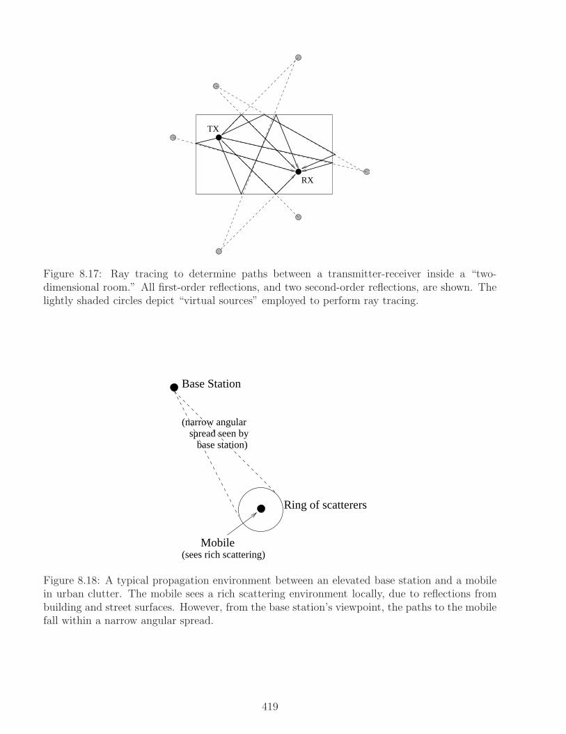
TX

RX

Figure 8.17: Ray tracing to determine paths between a transmitter-receiver inside a “two-dimensional room.” All first-order reflections, and two second-order reflections, are shown. Thelightly shaded circles depict “virtual sources” employed to perform ray tracing.

(sees rich scattering)

Base Station

Ring of scatterers

Mobile

(narrow angularspread seen by

base station)

Figure 8.18: A typical propagation environment between an elevated base station and a mobilein urban clutter. The mobile sees a rich scattering environment locally, due to reflections frombuilding and street surfaces. However, from the base station’s viewpoint, the paths to the mobilefall within a narrow angular spread.

419

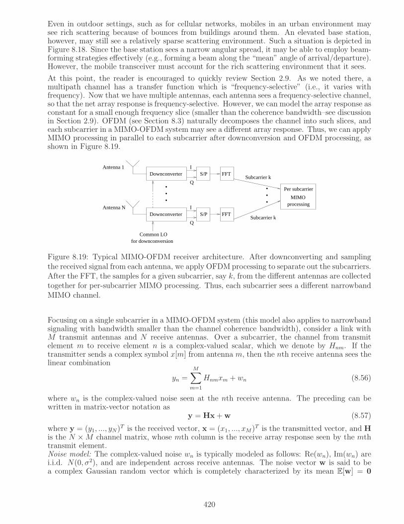
Even in outdoor settings, such as for cellular networks, mobiles in an urban environment maysee rich scattering because of bounces from buildings around them. An elevated base station,however, may still see a relatively sparse scattering environment. Such a situation is depicted inFigure 8.18. Since the base station sees a narrow angular spread, it may be able to employ beam-forming strategies effectively (e.g., forming a beam along the “mean” angle of arrival/departure).However, the mobile transceiver must account for the rich scattering environment that it sees.

At this point, the reader is encouraged to quickly review Section 2.9. As we noted there, amultipath channel has a transfer function which is “frequency-selective” (i.e., it varies withfrequency). Now that we have multiple antennas, each antenna sees a frequency-selective channel,so that the net array response is frequency-selective. However, we can model the array response asconstant for a small enough frequency slice (smaller than the coherence bandwidth–see discussionin Section 2.9). OFDM (see Section 8.3) naturally decomposes the channel into such slices, andeach subcarrier in a MIMO-OFDM system may see a different array response. Thus, we can applyMIMO processing in parallel to each subcarrier after downconversion and OFDM processing, asshown in Figure 8.19.

MIMO

S/P FFT

S/P FFT

.

.

....

Antenna N

Antenna 1

Downconverter

for downconversionCommon LO

DownconverterI

Q

I

Q

Subcarrier k

Subcarrier k

processing

Per subcarrier

Figure 8.19: Typical MIMO-OFDM receiver architecture. After downconverting and samplingthe received signal from each antenna, we apply OFDM processing to separate out the subcarriers.After the FFT, the samples for a given subcarrier, say k, from the different antennas are collectedtogether for per-subcarrier MIMO processing. Thus, each subcarrier sees a different narrowbandMIMO channel.

Focusing on a single subcarrier in a MIMO-OFDM system (this model also applies to narrowbandsignaling with bandwidth smaller than the channel coherence bandwidth), consider a link withM transmit antennas and N receive antennas. Over a subcarrier, the channel from transmitelement m to receive element n is a complex-valued scalar, which we denote by Hnm. If thetransmitter sends a complex symbol x[m] from antenna m, then the nth receive antenna sees thelinear combination

yn =

M∑

m=1

Hnmxm + wn (8.56)

where wn is the complex-valued noise seen at the nth receive antenna. The preceding can bewritten in matrix-vector notation as

y = Hx+w (8.57)

where y = (y1, ..., yN)T is the received vector, x = (x1, ..., xM)T is the transmitted vector, and H

is the N ×M channel matrix, whose mth column is the receive array response seen by the mthtransmit element.Noise model: The complex-valued noise wn is typically modeled as follows: Re(wn), Im(wn) arei.i.d. N(0, σ2), and are independent across receive antennas. The noise vector w is said to bea complex Gaussian random vector which is completely characterized by its mean E[w] = 0

420

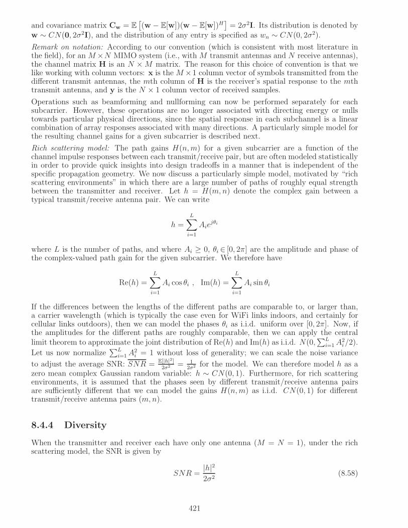
and covariance matrix Cw = E[

(w− E[w])(w − E[w])H]

= 2σ2I. Its distribution is denoted byw ∼ CN(0, 2σ2I), and the distribution of any entry is specified as wn ∼ CN(0, 2σ2).

Remark on notation: According to our convention (which is consistent with most literature inthe field), for anM×N MIMO system (i.e., withM transmit antennas and N receive antennas),the channel matrix H is an N ×M matrix. The reason for this choice of convention is that welike working with column vectors: x is theM ×1 column vector of symbols transmitted from thedifferent transmit antennas, the mth column of H is the receiver’s spatial response to the mthtransmit antenna, and y is the N × 1 column vector of received samples.

Operations such as beamforming and nullforming can now be performed separately for eachsubcarrier. However, these operations are no longer associated with directing energy or nullstowards particular physical directions, since the spatial response in each subchannel is a linearcombination of array responses associated with many directions. A particularly simple model forthe resulting channel gains for a given subcarrier is described next.

Rich scattering model: The path gains H(n,m) for a given subcarrier are a function of thechannel impulse responses between each transmit/receive pair, but are often modeled statisticallyin order to provide quick insights into design tradeoffs in a manner that is independent of thespecific propagation geometry. We now discuss a particularly simple model, motivated by “richscattering environments” in which there are a large number of paths of roughly equal strengthbetween the transmitter and receiver. Let h = H(m,n) denote the complex gain between atypical transmit/receive antenna pair. We can write

h =

L∑

i=1

Aiejθi

where L is the number of paths, and where Ai ≥ 0, θi ∈ [0, 2π] are the amplitude and phase ofthe complex-valued path gain for the given subcarrier. We therefore have

Re(h) =L∑

i=1

Ai cos θi , Im(h) =L∑

i=1

Ai sin θi

If the differences between the lengths of the different paths are comparable to, or larger than,a carrier wavelength (which is typically the case even for WiFi links indoors, and certainly forcellular links outdoors), then we can model the phases θi as i.i.d. uniform over [0, 2π]. Now, ifthe amplitudes for the different paths are roughly comparable, then we can apply the centrallimit theorem to approximate the joint distribution of Re(h) and Im(h) as i.i.d. N(0,

∑Li=1A

2i /2).

Let us now normalize∑L

i=1A2i = 1 without loss of generality; we can scale the noise variance

to adjust the average SNR: SNR = E[|h|2]2σ2 = 1

2σ2 for the model. We can therefore model h as azero mean complex Gaussian random variable: h ∼ CN(0, 1). Furthermore, for rich scatteringenvironments, it is assumed that the phases seen by different transmit/receive antenna pairsare sufficiently different that we can model the gains H(n,m) as i.i.d. CN(0, 1) for differenttransmit/receive antenna pairs (m,n).

8.4.4 Diversity

When the transmitter and receiver each have only one antenna (M = N = 1), under the richscattering model, the SNR is given by

SNR =|h|22σ2

(8.58)

421

Since h is a random variable, so is the SNR. In fact, since Re(h) and Im(h) are i.i.d. N(0, 12),

the sum of their squares is an exponential random variable (see Problems 5.11 and 5.21). Takinginto account the scaling by 2σ2, we can show that SNR is an exponential random variable withmean equal to the average SNR SNR = 1

2σ2 . If we now design our coded modulation strategyfor a nominal SNR of SNR0, we say that the system is in outage when the SNR is smaller thanthis value. The probability of outage is given by

Pout = P [SNR < SNR0] = 1− e−SNR0/SNR (8.59)

We would typically choose the nominal SNR, SNR0, to be smaller than the average SNR, SNR,by a link margin. For example, for a link margin of 10 dB, we have SNR0 = 0.1SNR, so thatPout = 1−e−0.1 ≈ 0.1 (for |x| small, ex ≈ 1+x for |x| small, so that 1−e−x ≈ x). Thus, even aftergiving up 10 dB in link margin, we still get a relatively high outage rate of 10%. Of course, thereis a nontrivial probability that the SNR with fading is higher than the nominal, hence we canhave negative link margins if we are willing to live with large enough outage rates. For example,a link margin of - 3 dB corresp that SNR0 = 2SNR, with outage rate Pout = 1 − e−2 = 0.865(too high for most practical applications).

In order to reduce the outage rate without increasing the link margin, we must employ diversity,which is a generic term used for any strategy that gets multiple, approximately independent,“looks” at a fading channel. We saw diversity in action for our simulation-based model inSoftware Lab 2.2. We now explore it for the rich scattering model, skipping some details in thederivation in the interest of arriving quickly at the key insights.

Benchmark: We continue to define our link margin relative to an unfaded single input singleoutput (SISO) system with average SNR of SNR = 1

2σ2 .

Receive diversity: Consider a receiver equipped with two antennas (N = 2). If they are spacedfar enough apart in a rich scattering environment, we can assume that the channel gains (for agiven subcarrier) seen by the two antennas are i.i.d. CN(0, 1) random variables. The receivedsamples at the two antennas are modeled as

yn = hnx+ wn , n = 1, 2

where x is the transmitted symbol, h[1], h[2] ∼ CN(0, 1) are i.i.d. (independent Rayleigh fading),and w[1], w[2] ∼ CN(0, 2σ2) are i.i.d. (independent noise samples). The optimal decision statisticis obtained using receive beamforming, and is given by

Z = h∗1y1 + h∗2y2 (8.60)

It can be shown that the SNR is now given by

SNR = G SNR (8.61)

where the gain relative to the benchmark SISO system is given by

G = |h1|2 + |h2|2 (8.62)

We can break this up into two gains: Gdiversity =|h1|2+|h2|2

2due to averaging channel fluctuations

across antennas, and Gcoh = 2 due to averaging noise across antennas (the signal terms arebeing combined coherently, so that the phases line up, while the noise terms are being combinedincoherently, across the two receive antennas). Thus,

G = GdiversityGcoh (8.63)

where Gdiversity =|h1|2+|h2|2

2and Gcoh = 2.

422

Equations (8.61) and (8.63) generalize directly to N receive antennas:

G = |h1|2 + ...+ |hN |2 = GdiversityGcoh

Gdiversity =|h1|2+...+|hN |2

N, Gcoh = N

(8.64)

As N gets large, the fluctuations due to fading get smoothed away, and Gdiversity → 1 by the lawof large numbers. In practice, however, even small values of N (e.g., N = 2, 4) give significantperformance gains.

−5 0 5 10 15 2010

−10

10−9

10−8

10−7

10−6

10−5

10−4

10−3

10−2

10−1

100

Link Margin (dB)

Out

age

Pro

babi

lity

1x11x21x4

Figure 8.20: Probability of outage versus link margin (dB) for receive diversity in 1×N MIMOsystems.

Suppose now that we design our coding and modulation so as to provide reliable performance ata nominal SNR, say SNR0, which is smaller than the SISO benchmark SNR by a link marginof L dB: SNR0(dB) = SNR(dB)− L(dB). The probability of outage is given by

Pout = P [SNR < SNR0] = P [G < 10−L(dB)/10] (8.65)

Figure 8.20 plots the outage probability as a function of link margin for several different valuesof N . The plots are obtained using the procedure outlined in Problem 8.12.

Transmit diversity: If the transmitter has multiple antennas, it can beamform towards thereceiver if it has implicit or explicit feedback regarding the channel, as already noted. Whensuch feedback is not available, we would like to use open loop strategies which provide diversity.Consider a system with a transmitter with two antennas, and a receiver with a single antenna(M = 2, N = 1). In a MIMO-OFDM system, for a given subcarrier, suppose that the transmitantenna 1 sends the sample x1 and transmit 2 sends the sample x2. If the transmitter knowsthe channel coefficients h1 and h2 from the two transmit antennas to the receive antenna, thenit could choose x1 = h∗1x, x2 = h∗2x, where x is the symbol to be transmitted. What do we dowhen h1 and h2 are unknown? In general, if we send x1, x2 from the two transmit elements, thenthe received sample is given by

y = h1x1 + h2x2 + w (8.66)

where w is noise. Thus, if x1 and x2 are two independent symbols, then they interfere with eachother at the receiver. On the other hand, if we set x1 = x2 = x/

√2 (normalizing the transmit

423

power across the two antennas to that of a transmitter with a single antenna), then we receive

y =h1 + h2√

2x+ w

If h1, h2 are i.i.d. CN(0, 1), it is easy to show that the effective channel coefficient heff = h1+h2√2

is also CN(0, 1). Thus, we still have Rayleigh fading, and have not made any progress relative toa single antenna transmitter! An ingenious solution to this problem is the Alamouti space-timecode (named after its inventor), which resolves the interference between the signals sent by thetwo transmit antennas over two time samples. Let s[1] and s[2] be two symbols to be transmitted.For a single antenna transmitter, they would be transmitted in sequence. For the two antennatransmitter now being considered, expanding the signal space dimension to two at the receiverby considering two successive time samples allows us to orthogonalize the contributions of thesetwo symbols at the receiver. Denoting by xi[1] and xi[2], i = 1, 2 the samples transmitted fromantenna i at two successive time intervals, we set

x1[1] = b[1]/√2, x2[1] = b[2]/

√2

x1[2] = −b∗[2]/√2, x2[2] = b∗[1]/

√2

(8.67)

where we have again normalized the net transmit power to that of a single antenna system.Figure 8.21 depicts the operation of the Alamouti space-time code, taking a sequence of symbolsas input, and mapping them in groups of two to a sequence of samples at the output of eachantenna.

b[1], b[2], b[3], b[4],...

b[1],−b*[2],b[3],−b*[4],...

b[2], b*[1], b[4], b*[3],...

Alamoutispace−time

code

Figure 8.21: The transmitter in an Alamouti space-time code takes two symbols at a time, andmaps them to two consecutive symbols to be sent from each of the two transmit antennas. Theinput to the space-time encoder is the sequence of symbols to be transmitted, b[n], while theoutputs are the sequences xi[n], i = 1, 2, to be transmitted from antenna i. The 1/

√2 factor

for power normalization is omitted from the figure.

The received samples in the two successive time intervals are given by

y[1] = h1x1[1] + h2x2[1] + w[1] = h1√2b[1] + h2√

2b[2] + w[1]

y[2] = h1x1[2] + h2x2[2] + w[2] = − h1√2b∗[2] + h2√

2b∗[1] + w[2]

(8.68)

We assume that the receiver has estimates of the channel coefficients h1 and h2 (e.g., using knowntraining signals). We would like to write the two observations as a received vector in which eachsymbol modulates a different signal vector. Since the symbols are conjugated when sent over thesecond time interval, we conjugate the second received sample when creating the received vector.This yields the following vector model:

y =

(

y[1]y∗[2]

)

= b[1]

(

h1√2

h∗2√2

)

+ b[2]

(

h2√2

− h∗1√2

)

+

(

w[1]w∗[2]

)

= b[1]u1 + b[2]u2 +w (8.69)

The vectors u1 =1√2(h1, h

∗2)

T and u2 =1√2(h2,−h∗1)T are orthogonal (i.e., uH

1 u2 = 0), regardless

of the values of the channel coefficients, hence the symbols b[1] and b[2] do not interfere with

424

each other. The vector w ∼ CN(0, 2σ2I). The optimal decision statistic Z[i] for symbol b[i] isgiven by matched filtering against ui:

Z[i] = uHi y, i = 1, 2 (8.70)

Exercise: Write out these decision statistics explicitly in terms of y[1], y[2], h1, h2.Answer: Z[1] = h∗1y[1] + h2y

∗[2], Z[2] = h∗2y[1]− h1y∗[2] (up to scale).

The SNR seen by each symbol is given by

SNRAlamouti =||ui||22σ2

=(|h1|2 + |h2|2)/2

2σ2= GAlamoutiSNR (8.71)

where

GAlamouti =(|h1|2 + |h2|2

2(8.72)

Comparing with (8.64) for receive diversity, we see that the Alamouti scheme in a 2 × 1 systemachieves the same diversity gain as receive diversity in a 1× 2 system, but does not provide thecoherent gain obtained from averaging across receive antennas in the latter. Of course, as we seein Problem 8.13 and in Software Lab 8.3, the Alamouti scheme applies to 2×N MIMO systemsfor arbitrary N , so that we can get noise averaging and receive diversity gains for N > 1. Theoutage rates computed in Problem 8.13 are plotted in Figure 8.22.

−5 0 5 10 15 2010

−16

10−14

10−12

10−10

10−8

10−6

10−4

10−2

100

Link Margin (dB)

Out

age

Pro

babi

lity

2x1 Alamouti2x2 Alamouti2x4 Alamouti

Figure 8.22: Probability of outage versus link margin (dB) for Alamouti space-time coding for2×N MIMO with rich scattering.

The simplicity of the Alamouti construction (and its optimality for 2× 1 MIMO) has led to itsadoption by a number of cellular and WiFi standards (just do an Internet search to see this).Unfortunately, the orthogonalization provided by the Alamouti space-time code does not scale tomore than two transmit antennas. There are a number of “quasi-orthogonal” constructions thathave been investigated, but these have had less impact on practice. Indeed, when there are alarge number of transmit antennas, the trend is to engineer the system so that the transmitter hasenough information about the channel to perform some form of transmit beamforming (possiblyusing multiple beams).

425

8.4.5 Spatial multiplexing

We have already seen that a transceiver with multiple antennas can use SDMA to communicatewith multiple nodes at different locations. For example, a cellular base station with multipleantennas can use the same time-frequency resources to send data streams in parallel to differentmobile devices (even if such devices only have one antenna each). When both transmitter andreceiver have multiple antennas, if the propagation environment is “rich enough,” then multipleparallel data streams can be sent between transmitter and receiver. This is termed spatialmultiplexing. Figure 8.23 depicts spatial multiplexing with two antennas, modeling, for example,one subcarrier in a MIMO-OFDM system. The per-stream symbol rate 1/T is the rate of sendingsymbols along a subcarrier, where T is the length of an OFDM symbol. With M-fold spatialmultiplexing, the aggregate symbol rate for a given subcarrier is M/T . This should be scaled upby the number of subcarriers to get the overall symbol rate.

per−stream symbol rate 1/T

parallel to

Serialb[1], b[2], b[3], b[4],...b[1],b[3],...

b[2],b[4],...aggregate symbol rate 2/T

Figure 8.23: For spatial multiplexing, the transmitter may take a sequence of incoming symbolsb[n], and do a serial-to-parallel conversion to map them to subsequences to be transmitted fromthe different antennas. In the example shown, the odd symbols are transmitted from antenna 1,and the even symbols from antenna 2. The aggregate symbol rate is twice the per-stream symbolrate.

For example, suppose that the transmitter and receiver in a MIMO-OFDM system each havetwo antennas (M = N = 2). For a given subcarrier in an OFDM system, consider a particulartime interval. Suppose that the transmitter sends x1 from antenna 1 and x2 from antenna 2(referring to Figure 8.23, x1 = b[1] and x2 = b[2] in the first time interval). The samples at thetwo receive elements are given by

y1 = H11x1 +H12x2 + w1

y2 = H21x1 +H22x2 + w2

which we can write in vector form as

y =

(

y1y2

)

= x1

(

H11

H21

)

+ x2

(

H12

H22

)

+

(

w1

w2

)

= x1u1 + x2u2 +w (8.73)

where u1 is the response seen by transmit element 1 at the two receive antennas, u2 is theresponse seen by transmit element 2 at the receive antennas, and w ∼ CN(0, 2σ2) is complexWGN. While we have considered a 2 × 2 MIMO system for illustration, the model is generallyapplicable for 2 × N MIMO systems with N ≥ 2, with u1 and u2 denoting the two columnsof the channel matrix H, corresponding to the received responses for each of the two transmitantennas, respectively.

In a MIMO-OFDM system, we have eliminated interference across subcarriers using OFDM, butwe have introduced interference in space by sending multiple symbols from different antennas.The vector spatial interference model (8.73) for each subcarrier is analogous to the vector timedomain interference model for ISI in singlecarrier systems discussed in Chapter 6. Just as we cancompensate for ISI using a time-domain equalizer if the time domain channel has appropriate

426

characteristics, we can compensate for spatial interference using a spatial equalizer if the spatialchannel has appropriate characteristics. For example, if u1 and u2 are linearly independent,then we can use linear ZF or MMSE techniques to demodulate the symbols x1 and x2. Thus,if there are M parallel data streams being sent from the transmit antennas, then we need atleast M receive antennas in order to obtain a signal space of large enough dimension for thelinear independence condition to be satisfied. Indeed, it can be shown more generally (withoutrestricting ourselves to ZF or MMSE techniques) that, for rich scattering models, the capacityof an M ×N MIMO channel scales as min(M,N), the minimum of the number of transmit andreceive antennas.

The ZF and MMSE receivers have been discussed in detail Section 8.2.2. For our purpose, therelevant expressions are those for complex-valued signals in (8.35). We reproduce the expressionfor ZF correlator here before adapting it to our present purpose.

cZF = C−1w U

(

UHC−1w U

)−1e

Recall that U is a matrix containing the signal vectors as columns, and that e is a unit vectorwith nonzero entry corresponding to the desired vector u0 in the ISI vector model (8.13). Inour spatial multiplexing model (8.73), U = H (the signal vectors are simply the columns ofthe channel matrix), the noise covariance Cw = 2σ2I, and we wish to demodulate the datacorresponding to both of the signal vectors. Letting e1 = (1, 0)T and e2 = (0, 1)T , the ZFcorrelators for the two streams can be written as (dropping scale factors corresponding to thenoise variance)

c1 = H(

HHH)−1

e1, c2 = H(

HHH)−1

e2

We can represent this compactly as a single ZF matrix CZF = [c1c2] containing these correlatorsare columns. Noting that [e1e2] = I, we obtain that

CZF = H(

HHH)−1

, ZF matrix for spatial demultiplexing (8.74)

The decision statistics for the multiplexed streams are given by

Z = CHZFy (8.75)

While we have focused on the 2× 2 example (8.73) in this derivation, it applies in general to Mspatially multiplexed streams in an M × N MIMO system with N ≥ M . The outage rate withzero-forcing reception for 2 × 2 and 2 × 4 is plotted in Figure 8.24, using software developed inProblem 8.14.

The MMSE receiver can be similarly derived to be

CMMSE =(

HHH + 2σ2I)−1

H, MMSE matrix for spatial demultiplexing (8.76)

where we have normalized the transmitted symbols to unit energy (E [|b[n]|2] = σ2b = 1).

It is interesting to compare the spatial multiplexing model (8.73) with the diversity model (8.69)for the Alamouti space-time code. The Alamouti code does not rely on the receiver havingmultiple antennas, and therefore uses time to create enough dimensions for two symbols to besent in parallel. Furthermore, the vectors u1 and u2 in the Alamouti model (8.69) are constructedsuch that they are orthogonal, regardless of the propagation channel. In contrast, the spatialmultiplexing model (8.73) relies on nature to provide vectors u1 and u2 that are “differentenough” to support two parallel symbols. We explore these differences in Software Lab 8.3. Thespectral efficiency of spatial multiplexing is twice that of the Alamouti code, but the diversitygain that it sees is smaller, as is evident from a comparison of the outage rate versus link margincurves in Figures 8.22 and 8.24. It is possible to systematically quantify the tradeoff betweendiversity and multiplexing, but this is beyond our scope here.

427

−10 0 10 20 30 40 50 6010

−6

10−5

10−4

10−3

10−2

10−1

100

Link Margin (dB)

Out

age

Pro

babi

lity

2x2 spatial mux2x4 spatial mux

Figure 8.24: Outage rate versus link margin (with respect to the SISO benchmark) for 2 × Nspatial multiplexing (N = 2, 4) with zero-forcing reception.


This chapter provides an introduction to modeling and equalization for communication overdispersive channels, including singlecarrier and OFDM modulation. All models and algorithmsare developed in complex baseband, so that upconversion and downconversion are not explicitlymodeled.

Modeling of singlecarrier systems• Symbols in a linearly modulated system pass through a cascade of the transmit, channel andreceive filters, where the cascade typically does not satisfy the Nyquist criterion for ISI avoidance.Any technique for handling the resulting ISI is termed equalization.• Receiver noise is modeled as AWGN passed through the receive filter.• Eye diagrams enable visualization of the effect of various ISI patterns, and equalization tech-niques are needed for reliable demodulation if the eye is closed.

Linear equalization• The decision statistic for a given symbol is computed by a linear operation on a vector ofreceived samples in an observation interval that is typically chosen to be large enough that itcontains a significant contribution from the symbol of interest. Observation intervals for succes-sive symbols are offset by the symbol time, so that the statistics of the desired symbol and theISI are identical across observation intervals.• The linear MMSE equalizer minimizes the MSE between the decision statistic and the desiredsymbol, and also maximizes the SINR over the class of linear equalizers.• The MSE and the MMSE equalizer can be expressed in terms of statistical averages, hencethe MMSE equalizer can be computed adaptively by replacing statistical averages by empiricalaverages. Such adaptive implementation requires transmission of a known training sequence.• The received vector over an observation interval is the sum of the desired symbol modulatinga desired vector, interfering symbols modulating interference vectors, plus a noise vector. Thisvector ISI model can be characterized completely if we know the transmit filter, the channelfilter, the receive filter, and the noise statistics at the input to the receive filter.

428

• Explicit analytical formulas can be given for the ZF and MMSE equalizer, and the associatedSINRs, once the vector ISI model is specified.• At high SNR, the MMSE equalizer tends to the ZF equalizer, which (for white noise) can be in-terpreted geometrically as projecting the received vector orthogonal to the interference subspacespanned by the interference vectors, thus nulling out the ISI while incurring noise enhancement.The ZF equalizer exists only if the desired vector is linearly independent of the interference vec-tors.• The geometric interpretation and analytical formulas for the ZF and MMSE equalizers devel-oped for white noise can be extended to colored noise, with the derivation using the concept ofnoise whitening.

OFDM• Since complex exponentials are eigenfunctions of any LTI system, multiple complex expo-nentials, each modulated by a complex-valued symbol, do not interfere with each other whentransmitted through a dispersive channel. Each complex exponential simply gets scaled by thechannel transfer function at that frequency. The task of equalization corresponds to undoing thiscomplex gain in parallel for each complex exponential. This is the conceptual basis for OFDM,which enables parallelization of the task of equalization even for very complicated channels bytransmitting along subcarriers.• OFDM can be implemented efficiently in DSP using an IDFT at the transmitter (frequencydomain symbols to time domain samples) and a DFT at the receiver (time domain samples tofrequency domain observations, which are the symbols scaled by channel gain and corrupted bynoise).• In order to maintain orthogonality across subcarriers (required for parallelization of the taskof equalization) when we take the DFT at the receiver, the effect of the channel on the trans-mitted samples must be that of a circular convolution. Since the physical channel correspondsto linear convolution, OFDM systems emulate circular convolution by inserting a cyclic prefix inthe transmitted time domain samples.

This section provides an initial exposure to how multiple antennas at the transmitter and receivercan be employed to enhance the performance of wireless systems. Three key techniques, whichin practice are combined in various ways, are beamforming, diversity and spatial multiplexing.

Beamforming and Nullforming• The array response for a linear array can be viewed as a mapping from the angle of ar-rival/departure to a spatial frequency.• For an N -element array, spatial matched filter, or beamforming, leads to a factor of N gain inSNR. For transmit beamforming in which each antenna element is transmitting at a fixed power,we obtain an additional power combining gain of N .• By forming a beam at a desired transceiver and nulls at other transceivers, an antenna arraycan support SDMA.

MIMO-OFDM abstraction• Decomposing a time domain channel into subcarriers using OFDM allows a simple model forMIMO systems, in which the channel between each pair of transmit and receive antennas ismodeled as a single complex gain for each subcarrier.• When the propagation environment is complex enough, the central limit theorem motivatesmodeling the channel gains between transmit-receive antenna pairs as i.i.d. zero mean complexGaussian random variables. We term this rich scattering model.• Under the rich scattering model, each transmit-receive antenna pair sees Rayleigh fading, butperformance degradation due to fading can be alleviated using diversity.

Diversity• Diversity strategies average over fades by exploiting roughly independent looks at the channel.• Receive spatial diversity using spatial matched filtering provides a channel averaging gain (av-eraging the fading gains across antennas) and a noise averaging gain (due to coherent combining

429

across antennas).• Transmit spatial diversity provides channel averaging gains alone. It is trickier than receive di-versity, since samples transmitted from different transmit antennas can interfere at the receiver.For two transmit antennas, the Alamouti space-time code is an optimal scheme for avoidinginterference between different transmitted symbols, while providing channel averaging gains.

Spatial multiplexing• Sending parallel data streams from different antennas increases the symbol rate proportionalto the number of data streams, with space playing a role analogous to bandwidth.• The parallel data streams interfere at the receiver, but can be demodulated using spatialequalization techniques analogous to the time domain equalization techniques studied in Chapter6 (e.g., suboptimal techniques such as ZF and MMSE).

8.6 Endnotes

While we have shown that ISI in singlecarrier systems can be handled using linear equalization,significant performance improvements can be obtained using nonlinear strategies, including op-timal maximum likelihood sequence estimation (MLSE), whose complexity is often prohibitivefor long channels and/or large constellations, as well as suboptimal strategies such as decisionfeedback equalization (DFE), whose complexity is comparable to that of linear equalization. Anintroduction to such strategies, as well as pointers for further reading, can be found in moreadvanced communication theory texts such as [7, 8].

OFDM has now become ubiquitous in both wireless and wireline communication systems in recentyears, because it provides a standardized mechanism for parallelizing equalization of arbitrarilycomplicated channels in a way that leverages the dropping cost and increasing speed of digitalcomputation. For more detail than we have presented here, we refer to the relevant chapters inbooks on wireless communication by Goldsmith [42] and Tse and Viswanath [43]. These shouldprovide the background required to access the huge research literature on OFDM, which focuseson issues such as channel estimation, synchronization and reduction of PAPR.

There has been an explosion of research and development activity in MIMO, or space-timecommunication, starting from the 1990s: this is the decade in which the large capacity gainsprovided by spatial multiplexing were pointed out by Foschini [44] and Telatar [45], and theAlamouti space-time code was published by Alamouti [46]. MIMO techniques have been in-corporated into 3G and 4G (WiMax and LTE) cellular standards, and WiFi (IEEE 802.11n)standards. An excellent reference for exploring MIMO-OFDM further is the textbook by Tseand Viswanath [43], while a brief introduction is provided in Chapter 8 of Madhow [7]. Otherbooks devoted to MIMO include Paulraj et al [47], Jafarkhani [48], and the compilation editedby Bolcskei et al [49].

As discussed in the epilogue, a new frontier in MIMO is opening up with research and developmentfor wireless communication systems at higher carrier frequencies, starting with the “millimeterwave” band (i.e., carrier frequencies in the range 30-300 GHz, for which the wavelength is in therange 1-10 mm). Of particular interest is the 60 GHz band, where there is a huge amount (7GHz!) of unlicensed spectrum, in contrast to the crowding in existing cellular and WiFi bands.While fundamental MIMO concepts such as beamforming, diversity, and spatial multiplexingstill apply, the order of magnitude smaller carrier wavelength and the order of magnitude largerbandwidth requires fundamentally rethinking many aspects of link and network design, as webriefly indicate in the epilogue.

430

8.7 Problems

ZF and MMSE equalization: modeling and numerical computations

Problem 8.1 (Noise enhancement computations) Consider the ISI vector models in (8.10),(8.12) and (8.11).(a) Compute the noise enhancements (dB) for the three equalizer lengths in these models, as-suming white noise.(b) Now, assume that the noise w[n] is colored, with Cw specified as follows:

Cw(i, j) =

σ2, i = jσ2

2, |i− j| = 1

0, else

(8.77)

Compute the noise enhancements for the three equalizer lengths considered, and compare withyour results in (a).

Problem 8.2 (Noise enhancement as a function of correlator length) Now, consider thediscrete time channel model leading to ISI vector models in (8.10), (8.12) and (8.11).(a) Assuming white noise, compute and plot the noise enhancement (dB) as a function of equalizerlength, for L ranging from 4 to 16, increasing the observation interval by two by adding one sampleto each side of the current observation interval, and starting from an observation interval of lengthL = 4 lined up with the impulse response for the desired symbol. Does the noise enhancementdecrease monotonically? Does it plateau? (b) Repeat for colored noise as in Problem 8.1(b).

Problem 8.3 (MMSE correlator and SINR computations) Consider the ISI vector model(8.10).

(a) Assume Cw = σ2I, and define SNR = ||u0||2σ2 as the MF bound on achievable SNR. For

SNR of 6 dB, compute the MMSE correlator and the corresponding SINR (dB), using (8.34)and (8.16). Check that the results match the alternative formula (8.36). Compare with the SNRachieved by the ZF correlator.(b) Plot the SINR (dB) of the MMSE and ZF correlators as a function of the MF SNR (dB).Comment on any trends that you notice.

n(t)

TX

t

1

0 1

g (t)C

t0

−0.5

2

−1

g (t)RX

t

1

0 1

Transmitfilter

Channelfilter

Receivefilter

Symbols

b[n]Sampler Samples

g (t)

Figure 8.25: Continuous time model for a link with ISI.

Problem 8.4 (From continuous time to discrete time vector ISI model) In this problem,we discuss an example of how to derive the vector ISI model (8.13) from a continuous time model,using the system shown in Figure 8.25. The symbol rate 1/T = 1, the input to the transmitfilter is

∑

n b[n]δ(t − nT ), where b[n]∈ −1, 1. Thus, the continuous time noiseless signal at

431

the output of the receive filter is∑

n b[n]q(t − nT ), where q(t) = (gTX ∗ gC ∗ gRX)(t) is thesystem response to a single symbol. The noise n(t) at the input to the receive filter is WGNwith PSD σ2 = N0

2, so that the noise w(t) = (n ∗ gRX)(t) at the output of the receive filter, using

the material in Section 5.9, is zero mean, WSS, Gaussian with autocorrelation/autocovariancefunction Rw(τ) = Cw(τ) = σ2(gRX ∗ gRX,mf )(τ).(a) Sketch the end-to-end response q(t). Compute the energy per bit Eb = ||q||2.Remark: Note that Eb

N0= ||q||2

2σ2 . If we fix the signal scaling, and hence ||q||2, then the value of σ2

is fixed once we specify Eb/N0.(b) Assume that the sampler operates at rate 2/T = 2, taking samples at times t = m/2 forinteger m. Show that the discrete time end-to-end response to a single symbol (i.e. the sampledversion of q(t)) is

h = (..., 0, 1, 2,−1

2,−1,−1

2, 0, ...)

(c) For the given sampling rate, show that a vector ISI model (8.13), the noise covariance matrixsatisfies (8.77).(d) Specify the matrix U corresponding to the ISI model (8.13) for a linear equalizer of length5, with observation interval lined up with the channel response for the desired symbol.(e) Taking into account the noise coloring, compute the optimal ZF correlator, and its noiseenhancement relative to the matched filter bound.(f) Compute the MMSE correlator for Eb

N0of 10 dB (see (a) and the associated remark). What

is the output SINR, and how does it compare with the SNR of the ZF correlator in (e)?

ZF and MMSE equalization: theoretical derivations

Problem 8.5 (ZF geometry) For white noise, the output of a ZF correlator satisfying (8.17)and (8.18) is given by

cT r[n] = b[n] +N(0, σ2||c||2)Since the signal scaling is fixed, the optimal ZF correlator is one that minimizes the noise varianceσ2||c||2. Thus, the optimal ZF correlator minimizes ||c||2 subject to (8.17) and (8.18).(a) Suppose a correlator c1 satisfies (8.17) and (8.18), and is a linear combination of the signalvectors uk. Now, suppose that we add a component ∆c orthogonal to the space spanned bythe signal vectors. Show that c2 = c1 +∆c is also a ZF correlator.(b) How is the output noise variance for c2 related to that for c1?(c) Conclude that, in order to be optimal, a ZF correlator must lie in the signal subspace spannedby uk.(d) Observe that the condition (8.17) implies that c must be orthogonal to the interferencesubspace spanned by uk, k 6= 0. Combining with (c), infer that c must be a scalar multiple ofP⊥

I u0.

Problem 8.6 (invertibility requirement for computing ZF correlator) The ZF correlatorexpression (8.22) requires inversion of the matrix UTU of correlations among the signal vectors,with (i, j)th entry ui,uj〉 = uT

i uj.(a) Show that

UTUa = 0 (8.78)

if and onlyUa = 0 (8.79)

Hint: In order to show that (8.78) implies (8.79), suppose that (8.78) holds. Multiply by aT andshow that you get an expression of the form xTx = ||x||2 = 0, which implies x = 0.(b) Use the result in (a) to infer that UTU is invertible if and only if the signal vectors uk arelinearly independent.

432

Problem 8.7 (Alternative computation of the ZF correlator) An alternative computa-tion for the ZF correlator is by developing an expression for P⊥

I u0 in terms of u0 and UI , amatrix containing the interference vectors uk, k 6= 0 as columns. That is, UI is obtained fromthe signal matrix U by deleting the column corresponding to the desired vector u0. Let us de-fine the projection of u0 onto the interference subspace by PIu0. By definition, this is a linearcombination of the interference vectors, and can be written as

PIu0 = UIaI (8.80)

The orthogonal projection P⊥I u0 is therefore given by

P⊥I u0 = u0 −PIu0 = u0 −UIaI (8.81)

(a) Note that bPperpu0 must be orthogonal to each of the interference vectors uk, k 6= 0, hence(going directly to the general complex-valued setting)

UHI P

⊥I u0 = 0

(b) Infer from (a) that

aI =(

UHI UI

)−1UH

I u0

(c) Derive the following explicit expression for the orthogonal projection

P⊥I u0 = u0 −UI

(

UHI UI

)−1UH

I u0 (8.82)

(d) Derive the following explicit expression for the energies of the projection onto the interferencesubspace and the orthogonal projection:

||PIu0||2 = uH0 UI

(

UHI UI

)−1UH

I u0

||P⊥I u0||2 = ||u0||2 − uH

0 UI

(

UHI UI

)−1UH

I u0 = uH0

(

I−UI

(

UHI UI

)−1UH

I

)

u0(8.83)

(e) Note that (8.82) and (8.83), together with (8.27), give us an expression for a ZF correlatorcZF scaled such that 〈cZF ,u0〉 = 1.

Problem 8.8 (Analytical expression for MMSE correlator) Let us derive the expression(8.34) for the MMSE correlator for the vector ISI model (8.13). We consider the general scenarioof complex-valued symbols and signals. Suppose that the symbols b[n] in the model areuncorrelated, satisfying

E[b[n]b∗[m]] =

0, m 6= nσ2b , m = n

(8.84)

We have

R = E[r[n]rH [n]] = E

[

(∑

k

b[n + k]uk +w[n])(∑

l

b[n + l]ul +w[n])H

]

p = E[b∗[n]r[n]] = E

[

b∗[n](∑

k

b[n+ k]uk +w[n])

]

Now use (8.84), and the independence of the symbols and the noise, to infer that

R = σ2b

∑

k

ukuHk +Cw , p = σ2

bu0

433

Problem 8.9 (ZF correlator for colored noise) Consider the model (8.13) where the noisecovariance is a positive definite matrix Cw. We now derive the formula (8.30) for the ZF corre-lator, by mapping, via a linear transformation, the system to a white noise setting for which wehave already derived the ZF correlator in (8.22). Specifically, suppose that we apply an invertiblematrix A to the received vector r[n], then we obtain a transformed received vector

r[n] = Ar[n] =∑

k

b[n + k]uk + w[n] (8.85)

where

uk = Auk (8.86)

w[n] = Aw[n] ∼ N(0,ACwAT ) (8.87)

(a) Suppose that we find a linear correlator c for the transformed system (8.85), leading to adecision statistic Z[n] = cT r[n]. Show that we can write the decision statistic Z[n] = cT r[n] (i.e.,as the output of a linear correlator operating on the original received vector), where

c = AT c (8.88)

(b) Suppose that we can find A such that the noise in the transformed system is white:

ACwAT = I (8.89)

Show that

C−1w = ATA (8.90)

(c) Show that the optimal ZF correlator c for the transformed system is given by

cZF = U(

UT U)−1

e (8.91)

(d) Show that the optimal ZF correlator cZF in the original system is given by (8.30).Hint: Use (8.86), (8.88) and (8.90).(e) While we have used whitening only as an intermediate step to deriving the formula (8.30) forthe ZF correlator in the original system, we note for completeness that a whitening matrix Asatisfying (8.89) is guaranteed to exist for any positive definite Cw, and spell out two possiblechoices for A. For example, we can take A = B−1, where B is the square root of Cw, whichis a symmetric matrix satisfying Cw = B2. Another, often more numerically stable, choice isA = L−1, where L is a lower triangular matrix obtained by the Cholesky decomposition of Cw.which satisfies Cw = LLT . Matlab functions implementing these are given below:

%square root of CwB=sqrtm(Cw); %symmetric matrix%Cholesky decomposition of CwL=chol(Cw,’lower’); %lower triangular matrix

Throughout the preceding problem, replacing transpose by conjugate transpose gives the cor-responding results for the complex-valued setting. The Matlab code segment above applies forboth real- and complex-valued noise.

434

MIMO

Problem 8.10 (Effect of array spacing) Consider a regular linear array with N elementsand inter-element spacing d.(a) For N = 8, plot the beam pattern for a beam directed at 30 from broadside for d = λ

4.

(b) Repeat (a) for d = 2λ.(c) Comment on any differences that you notice in the beamforming patterns in (a) and (b).(d) For inter-element spacings beyond αλ, the maximum of the beam pattern is not unique.That is, the beam pattern takes its maximum value not just in the desired direction, but alsoin a few other directions. These other maxima are called grating lobes. What is the value of αbeyond which you expect to see grating lobes?

Problem 8.11 (SDMA) The base station in a cellular network is equipped with a linear arraywith 16 elements uniformly spaced at λ/3. Consider two mobiles, Mobile A is at angle 20 frombroadside and Mobile B is at angle −30 from broadside.wishes to simultaneously send different data streams to two different mobiles. Assume that ithas a linear array with 16 elements uniformly spaced at λ/3. Mobile A is at angle 20 frombroadside and Mobile B is at angle −30 from broadside.(a) Compute the array responses corresponding to each mobile, and plot the beamforming pat-terns if the base station were only communicating with one mobile at a time.(b) Now, suppose that the base station employs SDMA using zero-forcing interference suppres-sion to send to both mobiles simultaneously. Plot the beam patterns used to send to Mobile Aand Mobile B, respectively.(c) What is the noise enhancement in (b) relative to (a).(d) Repeat (a)-(c) when Mobile B is at angle 10 from broadside (i.e., closer to Mobile A inangular spacing). You should notice a significant increase in noise enhancement.(e) Try playing around with different values of angular spacing between mobiles to determinewhen the base station should attempt to use SDMA (e.g., what is the minimum angular spacingat which the noise enhancement is, say, less than 3 dB).

Problem 8.12 (Outage rates with receive diversity) Consider a 1×N MIMO system withreceive diversity. The gain relative to a SISO system is given by (8.64):

G = |h1|2 + ...+ |hN |2

For our rich scattering model, hi ∼ CN(0, 1) are i.i.d., hence hi|2 are i.i.d. exponential randomvariables, each with mean one. We state without proof that the sum of N such random variablesis a Gamma random variable with PDF and CDF given by

pG(g) =gN−1

(N − 1)!e−gIg≥0 (8.92)

FG(g) = P [G ≤ g] = e−g∞∑

k=N

gk

k!= 1− e−g

N−1∑

k=0

gk

k!, g ≥ 0 (8.93)

(a) Use the preceding results to compute the probability of outage (log scale) for N -fold receivediversity versus link margin (dB) relative to the SISO benchmark for N = 1, 2, 4. That is,reproduce the results displayed in Figure 8.20.(b) Optional It may be an interesting exercise to use simulations to compute the empirical CDFof G, and to check that you get the same outage rate curves as those in (a).

435

Problem 8.13 (Alamouti scheme with multiple receive antennas) Consider a 2 × NMIMO system where the transmitter employs Alamouti space-time coding as in (8.67). LetH = (h1h2) denote the N × 2 channel matrix, with (N × 1) columns h1 and h2

(a) Show that the optimal receiver is given by (8.70), where u1 = 1√2(h1,h

∗2)

T and u2 =1√2(h2,−h∗

1)T , and

y =

(

y[1]y∗[2]

)

(b) Show that the SNR gain relative to our unfaded SISO system with the same transmit powerand constant channel gain of unity is given by

G =1

2

N∑

j=1

2∑

k=1

|H(j, k)|2

Comparing with the receive diversity gain (8.64) in a 1 × N system, answer the followingTrue/False questions (give reasons for your answers).(c) True or False: A 2× 2 MIMO system with Alamouti space-time coding is 3 dB better thana 1× 2 MIMO system with receive diversity.(d) True or False: A 2× 2 MIMO system with Alamouti space-time coding is 3 dB worse thana 1× 4 MIMO system with receive diversity.(e) Use the approach in Problem 8.12 to compute and plot the outage probability (log scale) ver-sus link margin (dB) relative to the unfaded SISO system for a 2×N MIMO system, N = 1, 2, 4.You should get a plot that follows those in Figure 8.22.

Problem 8.14 (Outage rates for spatial multiplexing with ZF reception) Consider two-fold spatial multiplexing in a 2 × N MIMO system with N × 2 channel matrix H. Define the2× 2 matrix R = HHH.(a) Referring to the spatial multiplexing model (8.73), how do the entries of R relate to thesignal vectors u1 and u2?(b) Show that the energy of the projection of u1 orthogonal to the subspace spanned by u2 isgiven by

E1 = R(1, 1)− |R(1, 2)|2R(2, 2)

where R(i, j) denotes the (i, j)th entry of R, i, j = 1, 2.(c) If we fix the transmit power to that of the SISO benchmark (splitting it equally between thetwo data streams), show that the gain seen by the first data stream is given by

G1 =E1

2=

1

2

(

R(1, 1)− |R(1, 2)|2R(2, 2)

)

Similarly, the gain seen by the second data stream is given by

G2 =1

2

(

R(2, 2)− |R(1, 2)|2R(1, 1)

)

Note that, under our rich scattering model, G1 and G2 are identically distributed random vari-ables.(c) Use computer simulations with the rich scattering model to plot the outage rate versus linkmargin for 2 × 2 and 2 × 4 MIMO with two-fold spatial multiplexing and ZF reception. Youshould get a plot similar to Figure 8.24. Discuss how the performance compares with that of theAlamouti scheme.

436

Problem 8.15 (Outage rates for spatial multiplexing with ZF reception) (a) Arguethat 2×N Alamouti space-time coding is exactly 3 dB worse than 1× 2N receive diversity.(b) For 2 × N spatial multiplexing with ZF reception, approximate its performance as x dBworse than a 1 × N ′ receive diversity. (Note that spatial multiplexing has twice the bandwidthefficiency as receive diversity, but it loses 3 dB of power up front due to splitting it between thetwo data streams.)Answer: Approximately 3 dB worse than 1×(N−1) receive diversity. That is, if the gain relativeto the SISO benchmark for a 1×N receive diversity system is denoted as Grx−div(N), then thegain for a 2×N spatial multiplexed system is Gsmux(N) ≈ 1

2Grx−div(N − 1)/2. Thus, the CDF,

and hence outage rate, of the spatially multiplexed system is approximated as

P [Gsmux(N) ≤ x] ≈ P [Grx−div(N − 1) ≤ 2x]

(c) Use the results in (b), and the analytical framework in Problem 8.12, to obtain an analyticalapproximation for the simulation results in Problem 8.14(c).

Software Lab 8.1: Introduction to Equalization in Singlecarrier Sys-

tems

Reading: Sections 8.1-8.2; Chapter 4 (linear modulation); Section 5.6 (Gaussian random vari-ables and the Q function). This lab can be completed without systematic coverage of Chapter6; we state and use probability of error expressions from Chapter 6, but knowing how they arederived is not required for the lab.

Lab Objectives: To understand the need for equalization in communication systems, and toimplement linear MMSE equalizers adaptively.


0) Use as your transmit and receive filters the SRRC pulse employed in Software Labs 4.1 and6.1. Putting the code for realizing these together with the code fragments developed in thischapter provides the code required for this lab. As in Software Labs 4.1 and 6.1, the transmit,channel, and receive filters are implemented at rate 4/T . For simplicity, we consider BPSKsignaling throughout this lab, and consider only real-valued signals. Generate nsymbols =ntraining+npayload (numbers to be specified later) ±1 BPSK symbols as in Lab 6.1, and passthem through the transmit, channel, and receive filters to get noiseless received samples at rate4/T .

1) Let us start with a trivial channel filter as before. Set nsymbols = 200. The number of rate4/T samples at the output of the receive filter is therefore 800, plus tails at either end becausethe length of the effective pulse modulating each symbol extends over multiple symbol intervals.Plot an eye diagram (e.g., using code fragment 8.1.3) using, say, 400 samples in the middle. Youshould get an eye diagram that looks like Figure 8.26: the cascade of the transmit and receivefilter is approximately Nyquist, and the eye is open, so that we can find a sampling time suchthat we can distinguish between +1 and -1 well, despite the influence of neighboring symbols.

2) Now introduce a non-trivial channel filter. In particular, consider a channel filter specified (atrate 4/T ) using the following matlab command:

channel filter = [−0.7,−0.3, 0.3, 0.5, 1, 0.9, 0.8,−0.7,−0.8, 0.7, 0.8, 0.6, 0.3]′;

Generate an eye diagram again. You should get something that looks like Figure 8.27. Noticenow that there is no sampling time at which you can clearly make out the difference between

437

0 0.2 0.4 0.6 0.8 1 1.2 1.4 1.6 1.8−10

−8

−6

−4

−2

0

2

4

6

8

10

Rec

eive

filte

r ou

tput

t/T

Figure 8.26: Eye diagram for a non-dispersive channel. The eye is open.

0 0.2 0.4 0.6 0.8 1 1.2 1.4 1.6 1.8−40

−30

−20

−10

0

10

20

30

Rec

eive

filte

r ou

tput

t/T

Figure 8.27: Eye diagram for a dispersive channel. The eye is closed.

438

+1 and -1 symbols. The eye is now said to be closed due to ISI, so that we cannot make symboldecisions just by passing appropriately timed received samples through a thresholding device.

3) We are now going to evaluate probability of error without and with equalization. First, letus generate the noisy output of the receive filter. We need to generate nsymbols = ntraining +npayload (numbers to be specified later)±1 BPSK symbols as in Software Lab 6.1, and pass themthrough the transmit filter, the dispersive channel, and the receive filter to get noiseless receivedsamples at rate 4/T . Since we are signaling along the real axis only, at the input to the receivefilter, add iid N(0, σ2) real-valued noise samples (as in lab 2, choose σ2 = N0

2corresponding to

a specified value of Eb

N0). Pass these (rate 4/T ) noise samples through the receive filter, and add

the result to the signal contribution at the receive filter output.

4) Performance without equalization: Let rk denote the output of the receive filter, andlet Z[n] = rd+4(n−1), n = 1, 2, ..., nsymbols denote the best symbol rate decision statistics youcan obtain by subsampling at rate 1/T the receive filter output. As in the solutions to earlierlabs, choose the decision delay d equal to the location of the maximum of the overall response(which now includes the channel) to a single symbol. For nsymbols = 10100, compute the error

probability of the decision rule b[n] = sign(Z[n]) as a function of Eb/N0, where the latter rangesfrom 5 to 20 dB. Compare with the ideal error probability curve for BPSK signaling for the samerange of Eb/N0. This establishes that a simple one-sample per symbol decision rule does notwork well for non-ideal channels, and motivates the equalization schemes discussed below.

Linear equalization: We now consider linear equalization, where the decision for symbol bn isbased on linear processing of a vector of samples r[n] of length L = 2M +1, where the entries ofr[n] are samples spaced by T/q, with the center sample being the same as the decision statisticin part 3: q = 1 corresponds to symbol-spaced sampling, and q > 1 corresponds to fractionallyspaced sampling. We consider two cases: q = 1 and q = 2.

r[n] = (rk+4(n−1)+d−(4/q)M , rk+4(n−1)+d−(4/q)(M−1), ...,rk+4(n−1)+d, rk+4(n−1)+d+(4/q),..., rk+4(n−1)+d+(4/q)M )T

The decision rule we use isb = sign(cT r[n]) (8.94)

where c is a correlator whose choice is to be specified. Note that the decision rule in part 3corresponds to the choice c = (0, .., 0, 1, 0, ..., 0)T , since it uses only the center sample.

The vector of samples r[n] contains contributions from both the desired symbol bn and from ISIdue to bn±1, bn±2, etc. We implement the linear minimum mean squared error (MMSE) equalizerusing a least squares adaptive implementation, as discussed in Section 8.2.1.

5) For the least squares implementation, assume that the first ntraining symbols are knowntraining symbols, b1, ..., bntraining. Define the L× L matrix

R =1

ntraining

ntraining∑

n=1

r[n]rT [n]

and the L× 1 vector

p =1

ntraining

ntraining∑

n=1

b[n]r[n]

The MMSE correlator is now approximated as

cMMSE = (R)−1p (8.95)

439

6) Now, the correlator obtained via (8.8) is used to make decisions, using the decision rule (8.94),on the unknown symbols n = ntraining + 1, ..., nsymbols.

7) Fix ntraining = 100 and npayload = 10000. For L = 3, 5, 7, 9, and q = 1, 2, implement linearMMSE equalizers, and plot their error probabilities (for the payload symbols) as a function ofEb/N0, in the range 5 to 20 dB. to the unequalized error probability and the ideal error probabilityfound in part 3.Hint: An efficient way to generate the statistics cT r[n] is to pass an appropriate rate 2/Tsubsequence of the receive filter output through a filter whose impulse response is the timereverse of c, and to then appropriately subsample at rate 1/T the output of the equalizing filter.This is much faster than correlating c with r[n] for each n.

8) Comment on the performance of symbol-spaced versus fractionally spaced equalization. Com-ment on the effect of equalizer length of performance. What is the effect of increasing or de-creasing the training period?

Lab Report: Your lab report should document the results of the preceding steps in order. Describethe reasoning you used and the difficulties you encountered.

Software Lab 8.2: Simplified Simulation Model for a OFDM link

Reading: Section 8.3; Chapter 4 (linear modulation).

Lab Objectives: To develop a hands-on understanding of basic OFDM transmission and re-ception.


We would like to leverage the code from Software Lab 8.1 as much as possible, so we set the DACfilter to be the transmit filter in that lab, and the receive filter to its matched filter as before.The main difference is that the time domain samples sent through the DAC filter are obtainedby taking the inverse FFT of the frequency domain symbols, and inserting a cyclic prefix. Wefix the constellation as Gray coded QPSK.

Step 1 (Exploring time and frequency domain relationships in OFDM): Let us firstdiscuss the structure of a single “OFDM symbol,” which carries N complex-valued symbols inthe frequency domain. Here N is the number of subcarriers, chosen to be a power of 2. Set L tobe length of the cyclic prefix. Set N = 256, L = 20 for these initial explorations, but keep theparameters programmable for later use.1a) Generate N Gray coded QPSK symbols B = B[k], k = 1, .., N. (You can use the functionqpskmap developed in Software Lab 6.1 for this purpose.) Take the inverse FFT to obtain timedomain samples b = b[n], n = 1, ..., N.1b) Append the last L time domain samples to the beginning, to get a length N + L sequenceof time domain samples b′ = b′[n], n = 1, ..., N + L. That is, b′[1] = b[N − L + 1], ..., b′[L] =b[N ], b′[L+ 1] = b[1], ..., b′[N + L] = b[N ].1c) Take the first N symbols of b′, say r1 = b′[1], ..., b′[N ]. Show that the FFT output (sayR1 = R1[k]) is related to the original frequency domain symbols B through a frequency domainchannel H as follows: R1[k] = H [k]B[k]. Find and plot the amplitude |H [k]| and phase arg(H [k])versus k.1d) Repeat 1c) for the time domain samples b′[3], ..., b′[N + 3] (i.e., skip the first two samplesof b′. How are the frequency domain channels in 1c) and 1d) related? (What we are doing hereis exploring what cyclic shifts in the time domain do in the frequency domain.)

Step 2 (generating multiple OFDM symbols): Now, we generate K frames, each carryingN Gray coded QPSK symbols. Set N = 256, L = 20, K = 5 for numerical results and plots in

440

this step.2a) For each frame, generate time domain samples and add a cyclic prefix, as in Steps 1a) and1b). Then, append the time domain samples for successive frames together. We now have astream of K(N +L) time domain samples, analogous to the time domain symbols sent in Lab 3.2c) Pass the time domain symbols through the same transmit filter (this is the DAC in Figure8.9) as in Software Labs 4.1, 6.1 and 8.1, again oversampling by a factor of 4. (That is, if thetime domain samples are at rate 1/Ts, the filter is implemented as rate 4/Ts. This gives us arate 4/Ts transmitted signal.2d) Compute the peak to average power ratio (PAPR) in dB for this transmitted signal (OFDMis notorious for having a large PAPR). This is done by taking the ratio of the maximum toaverage value of the magnitude squared of the time domain samples.2e) Note that the original QPSK symbols in the frequency domain have a PAPR of one, but thetime domain samples are generated by mixing these together. The time domain samples couldbe expected, therefore, to have a Gaussian distribution, invoking the central limit theorem. Plota histogram of the I and Q components from the time domain samples. Do they look Gaussian?2f) As in Lab 2, assume an ideal channel filter and pass the transmitted signal through a receivefilter matched to the transmit filter. This gives a rate 4/Ts noiseless received signal.2g) Subsample the received signal at rate 1/Ts, starting with a delay of d samples (play aroundand see what choice of d works well–perhaps based on the peak of the cascade of the transmit,channel and receive filter). The first N samples corresponding to the first frame. Take the FFTof these N samples to get R1[k]. Now, estimate the frequency domain channel coefficientsH [k] by using the known transmitted symbols B1[k] in the first frame as training. That is,

H[k] = R1[k]/B1[k]

Plot the magnitude and phase of the channel estimates and comment on how it compares towhat you saw in 1c) and 1d).2h) Now, use the channel estimate from 2g) to demodulate the succeeding frames. If frame muses time domain samples over a window [a, b], then frame m+1 uses time domain samples overa window [a + (N + L)Ts, b + (N + L)Ts]. Denoting the FFT of the time domain samples forframe m as Rm[k], the decision statistics for the frequency domain symbols for the mth frameare given by

Bm[k] = H∗[k]Rm[k]

You can now decode the bits and check that you get a BER of zero (there is no noise so far).Also, display scatter plots of the decision statistics to see that you are indeed seeing a QPSKconstellation after compensating for the channel.

Step 3 (Channel compensation): We now introduce a nontrivial channel (still no noise).Increase the cyclic prefix length if needed (it should be long enough to cover the cascade of thetransmit, channel and receive filters. But remember that the cyclic prefix is at rate 1/Ts, whereasthe filter cascade is at rate 4/Ts.3a) Repeat Step 2f, but now with a nontrivial channel filter modeled at rate 4/Ts. Use thechannels you have tried out in Lab 3 (still no noise). For example:

channel filter = [−0.7,−0.3, 0.3, 0.5, 1, 0.9, 0.8,−0.7,−0.8, 0.7, 0.8, 0.6, 0.3]′;

3b) Repeat Step 2g. Comment on how the magnitude and phase of the frequency domain channeldiffers from what you saw in 2g, 1c and 1d.3c) Repeat Step 2h. Check that you get a BER of zero, and that your decision statistics givenice QPSK scatter plots.3d) Check that everything still works out as you vary the number of subcarriers N (e.g., N =512, 1024, 2048), the cyclic prefix length L and the number of frames K.

Step 4 (Effect of noise): Now, add noise as in Software Labs 6.1 and 8.1. Specifically, at theinput to the receive filter, add independent and identically distributed (iid) complex Gaussian

441

noise, such that the real and imaginary part of each sample are iid N(0, σ2) (we choose σ2 = N0

2

corresponding to a specified value of Eb

N0). Let us fix N = 1024 for concreteness, and set the cyclic

prefix to just a little longer than the minimum required for the channel you are considering. Setthe number of frames to K = 10. Try a couple of values of Eb/N0 of 5 dB and 8 dB.4a) While you can estimate Eb analytically, estimate it by taking the energy of the transmittedsignal in 3a, and dividing it by the number of bits in the payload (i.e., excluding the first frame).Use this to set the value of N0 for generating the noise samples.4b) Pass the (rate 4/Ts) noise samples through the receive filter, and add the result to the outputof part 3a.4c) Consider first a noiseless channel estimate, in which you carry out Step 3b (estimating thechannel based on frame 1) before you add noise to the output of 3a. Now add the noise andcarry out Step 3c (demodulating the other frames). Estimate the BER and compare with theanalytical value for ideal QPSK. Show the scatter plots of the decision statistics.4d) Repeat 4c, except that you now estimate the channel based on frame 1 after adding noise.Discuss how the BER degrades. Compare the channel estimates from parts 4c and 4d on thesame plot.Note: You may notice a significant BER degradation, but that is because the channel estimationtechnique is naive (the channel coefficients for neighboring subcarriers are highly correlated, butour estimate is not exploiting this property). Exploring better channel estimation techniques isbeyond the scope of this lab, but you are encouraged to browse the literature on OFDM channelestimation to dig deeper.

Step 5 (Consolidation): Once you are happy with your code, plot the BER (log scale) as afunction of Eb/N0 (dB) for the channel in Lab 3. Plot three curves: ideal QPSK, OFDM withnoiseless channel estimation, OFDM with noisy channel estimation. Comment on the relationbetween the curves.


Software Lab 8.3: MIMO signal processing

Reading: Section 8.4

Lab Objectives: To gain hands-on exposure to basic MIMO signal processing at the transmitterand receiver.


Background: Consider the rich scattering model for a single subcarrier in a MIMO-OFDMsystem with M transmit and N receive antennas. The N ×M channel matrix H is modeled ashaving i.i.d. CN(0, 1) entries.

Code Fragment 8.7.1 (MIMO matrix with i.i.d. complex Gaussian entries)

%M,N specified earlier%MIMO matrix with iid CN(0,1) entriesH=(randn(N,M)+j*randn(N,M))/sqrt(2);

Let T denote the number of time domain samples for our system. Let xi[t] denote the sam-ple transmitted from transmit antenna i at time t, where 1 ≤ i ≤ M and 1 ≤ t ≤ T . Letx[t] = (x1[t], ..., xM [t])T denote the M × 1 vector of samples transmitted at time t, and let

442

X = (x[1], ...,x[T ]) denote the M × T matrix containing all the transmitted samples. Our con-

vention is to normalize the net transmit power to one, so that |xi[t]|2 = 1M. For a single input

single output (SISO) system, this would lead to an average received SNR of SNR = 12σ2 , since the

magnitude squared of the channel gain is normalized to one, and the noise per receive antennais modeled as CN(0, 2σ2), and we vary this hypothetical SISO system SNR when evaluatingperformance.

The N × T received matrix Y, with yj [t], 1 ≤ j ≤ N denoting the spatial vector of receivedsamples at time t, is then modeled as

Y = HX+N

where N is an N × T matrix with i.i.d. CN(0, 2σ2) entries. This model is implemented in thefollowing code fragment.

Code Fragment 8.7.2 (Received signal in MIMO system)

%snrbardb specified earlier%express snrbar in linear scalesnrbar = 10^(snrbardb/10);%find noise variance, assuming TX power = 1%(snrbar = 1/(2*sigma^2))sigma = sqrt(1/(2*snr));%x = MxT vector of symbols, already specified earlier%(normalized to unit power per time)%%RECEIVED SIGNAL MODEL: N x T matrixy=H*x + sigma*randn(N,T)+j*sigma*randn(N,T);

In order to use the preceding generic code fragments for a particular MIMO scheme, we must(a) map the transmitted symbols into the matrix X of transmitted samples, and (b) process thematrix Y of received samples appropriately.

Alamouti space-time code: We first consider the Alamouti space-time code for a 2×1 MIMOsystem. The transmitted samples can be generated using the following code fragment.

Code Fragment 8.7.3 (Transmitted samples for Alamouti space-time code)

%assume number of time samples T has been specified%QPSK symbols normalized to unit power per symbolsymbols= (sign(rand(1,T) - 0.5)+j*sign(rand(1,T) - 0.5))/sqrt(2);%Alamouti space-time code mappingX=zeros(2,T); %M=2X(1,1:2:T) = symbols(1:2:T); %odd samples from antenna 1X(2,1:2:T) = symbols(2:2:T);%odd samples from antenna 2X(1,2:2:T) = -conj(symbols(2:2:T));%even samples from antenna 1X(2,2:2:T)= conj(symbols(1:2:T)); %even samples from antenna 2

Step 1: Consider a 2 × 1 MIMO system. Setting M = 2, N = 1 and SNR at 10 dB, put codefragments 8.7.1, 8.7.3, and 8.7.2 together to model the transmitted and received matrices X andY. Setting T = 100, do a scatter plot of the real and imaginary parts of the received samples.The received samples should be smeared out over the complex plane, since the signals from thetwo transmit antennas interfere with each other at the receive antenna.

Step 2: Compute the decision statistics (8.70) based on the received matrix Y. You may usethe following code fragment, but you must explain what it is doing. Do a scatter plot of thedecision statistics. You should recover the noisy QPSK constellation.

443

Code Fragment 8.7.4 (Receiver processing for Alamouti space-time code for a 2× 1MIMO system)

Ytilde = zeros(2,T/2); %assume T evenYtilde(1,:) = Y(1,1:2:T);Ytilde(2,:) = conj(Y(1,2:2:T));%u1= [H(1,1);conj(H(1,2))]; u2 = [H(1,2);-conj(H(1,1))];u1= [H(1,1);conj(H(1,2))]; u2 = [H(1,2);-conj(H(1,1))];Z(1:2:T) = u1’*Ytilde;Z(2:2:T) = u2’*Ytilde;

Step 3: Repeat Steps 1 and 2 for a few different realizations of the channel matrix. The quality

of the scatter plot in Step 2 should depend on the G = |H(1,1)|2+|H(1,2)|22

.

Step 4: Now, suppose that we use the Alamouti space-time code for a 2 × N MIMO system,where N may be larger than one. Show that only the receiver processing code fragment 8.7.4needs to be modified (other than changing the value of N in the other code fragments), with

Y having dimension 2N × T2

and u1, u2 each having dimension 2N × 1. Implement thesemodifications and do a scatter plot of the decision statistics for N = 2 and N = 4, fixing theequivalent SISO SNR to 10 dB. You should notice a qualitative improvement with increasing Nas you run several channel matrices, although the plots depend on the channel realization.Hint: See Problem 8.13.

We now consider spatial multiplexing in a 2×N MIMO system. We can now send 2T symbolsover T time intervals, as in the following code fragment.

Code Fragment 8.7.5 (Transmitted samples for two-fold spatial multiplexing)

%QPSK symbols normalized to unit powersymbols= (sign(rand(1,2*T) - 0.5)+j*sign(rand(1,2*T) - 0.5))/sqrt(2);x=zeros(M,T);%normalize samples so as emit unit power per unit timex(1,:) = symbols(1:2:2*T)/sqrt(2);x(2,:) = symbols(2:2:2*T)/sqrt(2);

Step 5: Setting M = 2, N = 4 and SNR at 10 dB, put code fragments 8.7.1, 8.7.5, and 8.7.2together to model the transmitted and received matrices X and Y. Setting T = 100, again doa scatter plot of the real and imaginary parts of the received samples for each received antenna.As before, the received samples should be smeared out over the complex plane, since the signalsfrom the two transmit antennas interfere with each other at the receive antennas.

Step 6: Now, apply a ZF correlator as in (8.74) to Y to separate the two data streams. Doscatter plots of the two estimated data streams. You should recover noisy QPSK constellations.

Step 7: Fixing SNR at 10 dB and fixing a 2 × 4 channel matrix, compare the scatter plotsof the decision statistics for the Alamouti scheme with those for two-fold spatial multiplexing.Which ones appear to be cleaner?


444

Epilogue

We conclude with a brief discussion of research and development frontiers in communicationsystems. This discussion is speculative by its very nature (it is difficult to predict progressin science and technology) and is significantly biased by the author’s own research experience.There is no attempt to be comprehensive. The goal is to highlight a few of the exciting challengesin communication systems in order to stimulate the reader to explore further.

The Continuing Wireless Story

The growth of content on the Internet continues unabated, driven by applications such as video-on-demand, online social networks, and online learning. At the same time, there have beensignificant advances in the sophistication of mobile devices such as smart phones and tabletcomputers, which greatly enhance the quality of the content these devices can support (e.g.,smart phones today provide high-quality displays for video on demand). As a result, usersincreasingly expect that Internet content is ubiquitously and seamlessly available on their mobiledevice. This means that, even after the runaway growth of cellular and WiFi starting in the1990s, wireless remains the big technology story. Mobile operators today face the daunting taskof evolving networks originally designed to support voice into broadband networks supplying datarates of the order of 10s of Mbps or more to their users. By some estimates, it requires a 1000-foldincrease in cellular network capacity in urban areas! On the other hand, since charging by thebyte is not an option, this growth in capacity must be accomplished in an extremely cost-effectivemanner, which demands significant technological breakthroughs.

At the other end of the economic spectrum, cellular connectivity has reached the remotest cornersof this planet, with even basic voice and text messaging transforming lives in developing nationsby providing access to critical information (e.g., enabling farmers to obtain timely information onmarket prices and weather). The availability of more sophisticated mobile devices implies thatongoing revolutionary developments in online education and healthcare can reach underservedpopulations everywhere, as long as there is adequate connectivity to the Internet. The lack ofsuch connectivity is commonly referred to as the digital divide.

Wireless researchers now face the challenge of building on the great expectations created by thesuccess of the technologies they have created. At one end, how can we scale cellular networkcapacity by several orders of magnitude, in order to address the exponential growth in demandfor wireless data created by smart mobile devices? At the other extreme, how do we close thedigital divide, ensuring that even the most remote regions of our planet gain access to the wealthof information available online? In addition, there are a number of specialized applications ofwireless that may assume significant importance as time evolves.

We summarize some key concepts driving this continuing technology story in the following.

Small cells: There are two fundamental approaches to scaling up data rates: increasing spatialreuse (i.e., using the same time-bandwidth resources at locations that are far enough apart),and increasing communication bandwidth. Decreasing cell sizes from macrocells with diameters

445

of the order of kilometers to picocells with diameters of the order of 100-200 meters increasesspatial reuse, and hence potentially the network capacity, by two orders of magnitude. Picocel-lular base stations may be opportunistically deployed on lampposts or rooftops, and see a verydifferent propagation and interference environment from macrocellular base stations carefullyplaced at elevated locations. Interference among adjacent picocells becomes a major bottleneck,as does the problem of handing off rapidly moving users as they cross cell boundaries (indeed,cell boundaries are difficult to even define in picocellular networks due to the complexity ofbelow-rooftop propagation). Thus, it is important to rethink the design philosophy of tightlycontrolled deployment and operation in today’s macrocellular networks. The scaling and organicgrowth of picocellular networks is expected to require a significantly greater measure of decentral-ized self-organization, including, for example, auto-configuration for plug-and-play deployment,decentralized coordination for interference and mobility management, and automatic fault de-tection and self-healing. Another critical issue with small cells is backhaul (i.e., connecting eachbase station to the wired Internet): pulling optical fiber to every lamppost on which a picocel-lular base station is deployed may not be feasible. Finally, we can go to even smaller cells calledfemtocells, with base stations typically deployed indoors, in individual homes or businesses, andusing the last mile broadband technology already deployed in such places for backhaul. For bothpicocells and femtocells, it is important to devise efficient techniques for sharing spectrum, andmanaging potential interference, with the macrocellular network. In essence, we would like tobe able to opportunistically deploy base stations as we do WiFi access points, but coordinatejust enough to avoid the tragedy of the commons resulting from the purely selfish behavior inunmanaged WiFi networks. Of course, as we learn more about how to scale such self-organizedcellular networks, we might be able to apply some of the ideas to promote peaceful coexistencein densely deployed and independently operated WiFi networks using unlicensed spectrum. Inshort, it is fair to say that there is a clear opportunity and dire need for significant innovations inoverall design approach as well as specific technological breakthroughs, in order to truly attainthe potential of “small cells.”

Millimeter wave communication: While commercial wireless networks deployed today employbands well below 10 GHz, there is significant interest in exploring higher carrier frequencies, wherethere are vast amounts of spectrum. Of particular interest are millimeter (mm) wave frequenciesfrom 30-300 GHz, corresponding to wavelengths from 10 mm down to 1 mm. Historically,RF front end technology for these bands has been expensive and bulky, hence there was limitedcommercial interest in using them. This has changed in recent years, with the growing availabilityof low-cost silicon radio frequency integrated circuits (RFICs) in these bands. The particular sliceof spectrum that has received the most attention is the 60 GHz band (from 57-64 GHz). Most ofthis band is unlicensed worldwide. The availability of 7 GHz of unlicensed spectrum (vastly morethan the bandwidth in current cellular and WiFi systems) opens up the possibility for anotherrevolution in wireless communication, with links operating at multiples of Gigabits per second(Gbps). Potential applications of 60 GHz in particular, and mm wave in general, include order ofmagnitude increases in the data rates for indoor wireless networks, multiGbps wireless backhaulnetworks, and base station to mobile links in picocells, and even wireless data centers. However,realizing the vision of multiGbps wireless everywhere is going to take some work. While we candraw upon the existing toolkit of ideas developed for wireless communication to some extent,we may have to rethink many of these ideas because of the unique characteristics of mm wavecommunication. The latter largely follow from the order of magnitude smaller carrier wavelengthrelative to existing wireless systems.

At the most fundamental level, consider propagation loss. As discussed in Section 6.5 (see alsoProblems 6.37 and 6.38), the propagation loss for omnidirectional transmission scales with thesquare of the carrier frequency, but for the same antenna aperture, antenna directivity scalesup with the square of the carrier frequency. Thus, given that generating RF power at highcarrier frequencies is difficult, we anticipate that mm wave communication systems will employantenna directivity at both ends. Since the inter-element spacing scales with carrier wavelength,

446

it becomes possible to accommodate a large number of antenna elements in a small area (e.g.,a 1000 element antenna array at 60 GHz is palm-sized!), and use electronic beamsteering torealize pencil beams at the transmitter and receiver. Of course, this is easier said than done.Hardware realization of such large arrays remains a challenge. On the algorithmic side, sincebuilding a separate upconverter or downconverter for every antenna element is infeasible as wescale up the array, it is essential to devise signal processing algorithms that do not assume theavailability of the separate complex baseband signals for each antenna element. The natureof diversity and spatial multiplexing also fundamentally changes at tiny wavelengths: due tothe directionality of mm wave links, there are only a few dominant propagation paths, so thatdesigns for rich scattering models no longer apply. For indoor environments, blockage by humansand furniture becomes inevitable, since the ability of electromagnetic waves to diffract aroundobstacles depends on how large they are relative to the wavelength (i.e., obstacles “look bigger”at tiny wavelengths). For outdoor environments, performance is limited by the oxygen absorptionloss (about 16 dB/km) in the 60 GHz band, and rain loss for mm wave communication in generaland the mm wave band (e.g., as high as 30 dB/km in heavy rain). While link ranges of hundredsof meters can be achieved with reasonable margins to account for these effects, longer rangesthan these would be fighting physics, hence multihop networks become interesting. Of course,once we start forming pencil beams, networking protocols that rely on the broadcast natureof the wireless medium no longer apply. These are just a few of the issues that are probablygoing to take significant research and development to iron out, which bodes well for aspiringcommunication engineers.

Figure 8.28 depicts how picocells and mm wave communication might come together to addressthe cellular capacity crisis. A large macrocellular base station provides default connectivityvia Long Term Evolution (LTE), a fourth generation cellular technology standardized relativelyrecently; despite its name, it may not suffice for the long term because of exponentially increasingdemand. Picocellular base stations are deployed opportunistically on lampposts, and may beconnected via a mm wave backhaul network. Users in a picocell could talk to the base stationsusing LTE, or perhaps even mm wave. Users not covered by picocells talk to the macrocell usingLTE.

Cooperative communication While we have studied communication between a single transmitterand receiver in this book, it provides a building block for emerging ideas in cooperative communi-cation. For example, neighboring nodes could form a virtual antenna array, forming distributedMIMO (DMIMO) systems with significantly improved power-bandwidth tradeoffs. This allowsus, for example, to bring the benefits of MIMO to systems with low carrier frequencies whichpropagate well over large distances, but are not compatible with centralized antenna arrays be-cause of the large carrier wavelength. For example, the wavelength at 50 MHz is 6 meters, henceconventional antenna arrays would be extremely bulky, but neighboring nodes naturally spacedby tens of meters could form a DMIMO array. DMIMO at low carrier frequencies is a promisingapproach for bridging the digital divide in cost-effective fashion, providing interference suppres-sion and multiplexing capabilities as in MIMO, along with link ranges of tens of kilometers.Another promising example of cooperative communication is interference alignment, in whichmultiple transmitters, each of which is sending to a different receiver, coordinate so as to ensurethat the interference they generate for each other is limited in time-frequency space. Of course,realizing the benefits of cooperative communication require fundamental advances in distributedsynchronization and channel estimation, along with new network protocols that support theseinnovations. More good news for the next generation of communication engineers!

Full-duplex communication: Most communication transceivers cannot transmit and receive atthe same time on the same frequency band (or even closely spaced bands). This is because evena small amount of leakage from the transmit chain can swamp out the received signal, which ismuch weaker. Thus, communication networks typically operate in time division duplexed (TDD)mode (also more loosely termed half duplex mode), in which the transmitter and receiver use thesame band, but are not active at the same time, or in frequency division duplexed (FDD) mode,

447

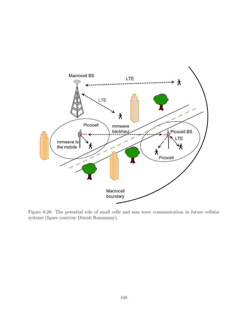
Figure 8.28: The potential role of small cells and mm wave communication in future cellularsystems (figure courtesy Dinesh Ramasamy).

448

in which the transmitter and receiver may be simultaneously active, but in different, typicallywidely separated, bands. There has been promising progress recently, however, on relatively low-cost approaches to canceling interference from the transmit chain, seeking to make full duplexoperation (i.e., sending and receiving at the same time in the same band) feasible. If thesetechniques turn out to be robust and practical, then they could lead to significant performanceenhancements in wireless networks. Of course, networking with full duplex links require revisitingcurrent protocols, which are based on either TDD or FDD.

Challenging channels: While we have discussed issues related to significant improvements inwireless data rates and ranges relative to large-scale commercial wireless networks today, thereare important applications where simply forming and maintaining a viable link is a challenge.Examples include underwater acoustic networks (for sensing and exploration in oceans, riversand lakes) and body area networks (for continuous health monitoring).

Wireless-enabled multi-agent systems: Wireless is at the heart of many emerging systems thatrequire communication and coordination between a variety of “agents” (these may be machinesor humans). Examples include asset tracking and inventory management using radio frequencyidentification (RFID) tags; sensor networks for automation in manufacturing, environmentalmonitoring, healthcare and assisted living; vehicular communication; smart grid; and nascentconcepts such as autonomous robot swarms. Such “multi-agent” systems rely on wireless toprovide tetherless connectivity among agents, as well as to possibly provide radar-style measure-ments, hence characterization and optimization of the wireless network in each specific contextis essential for sound system design.

Scaling mostly digital transceivers

As discussed in Chapter 1, a key technology story that has driven the growth of communicationsystems is Moore’s law, which allows us to inexpensively implement sophisticated DSP algorithmsin communication transceivers. A modern “mostly digital” receiver typically has analog-to-digital converters (ADCs) representing each I and Q sample with 8-12 bits of precision. Ascommunication data rates and bandwidths increase, Moore’s law will probably be able to keepup for a while longer, but the ADC becomes a bottleneck as signal bandwidths, and hencethe required sampling rates, scale to GHz and beyond. High-speed, high-precision ADCs arepower-hungry, occupy large chip areas (and are therefore expensive), and are difficult to build.Thus, a major open question in communication systems is whether we can continue to enjoy theeconomies of scale provided by “mostly digital” architectures as communication bandwidths goup.

We have already discussed the potential for mm wave communication and its unique challenges.The ADC bottleneck is one more challenge we must add to the list, but this challenge appliesto any communication system which seeks to employ DSP while scaling up bandwidth. Animportant example is fiber optic communication, where the bandwidths involved are huge. Forthe longest time, these systems have operated using elementary signaling schemes such as on-offkeying, with mostly analog processing at the receiver. However, researchers are now seeking tobring the sophistication of wireless transceivers to optical communication. By making opticalcommunication more spectrally efficient, we can increase data rates on fibers already buried in theground, simply by replacing the transceivers at each end. Sophisticated algorithms are criticalfor achieving this, and these are best implemented in DSP. Furthermore, by making opticaltransceivers mostly digital, we could obtain the economies of scale required for high-volumeapplications such as very short-range chip-to-chip, or intra-chip, communication. Comparedto wireless communication, optical communication represents special challenges due to fibernonlinearities and because of its higher bandwidth, while not facing the difficulties arising frommobility.

449

Yet another area where we seek increased speed and sophistication is wired backplane commu-nication for interconnecting hardware modules on a circuit board (e.g., inputs and outputs for ahigh-speed router, or processor and memory modules in computer), and “networks on chip” forcommunicating between modules on a single integrated circuit (e.g., for a “multi-core” processorchip with multiple processor and memory modules).

How does one overcome the ADC bottleneck? We do not have answers yet, but there are somenatural ideas to try. One possibility is to try and get by with fewer bits of precision per sample.Severe quantization introduces a significant nonlinearity, but it is possible that we could stillextract enough information for reliable communication if the dynamic range of the analog signalbeing quantized is not too large. Of course, the algorithms that we have seen in this textbook(e.g., for demodulation, linear equalization, MIMO processing) all rely on the linearity of thechannel not being disturbed by the ADC, an excellent approximation for high-precision ADC.This assumption now needs to be thrown out: in essence, we must “redo” DSP for communicationif we are going to live with low-precision ADC at the receiver. Another possibility is to parallelize:we could implement a high-speed ADC by running lower speed ADCs in parallel, or we coulddecompose the communication signal in the frequency domain, such that relatively low-speedADCs with high precision can be used in parallel for different subbands. These are areas ofactive research.

Beyond Moore’s law

Moore’s law has been working because the semiconductor industry keeps managing to shrinkfeature sizes on integrated circuits, making transistors (which are then used as building blocksfor digital logic) tinier and tinier. Many in the industry now say that the time is approachingwhen shrinking transistors in this fashion will make their behavior non-deterministic (i.e., theiroutput can have errors, just like the output of a demodulator in a communication system). Doingdeterministic logic computations with non-deterministic units is a serious challenge, which looksto be more difficult than reliable communication over a noisy channel. However, it is an intriguingquestion as to whether it is possible to use ideas similar to those in digital communication toevolve new paradigms for reliable computation with unreliable units. This is a grand challengeto which experts in communication systems might be able to make significant contributions.

Parting thoughts

The introductory treatment in this textbook is intended to serve as a gateway to an exciting futurein communications research and technology development. We hope that this discussion gives thereader the motivation for further study in this area, using, for example, more advanced textbooksand the research literature. We do not provide specific references for the topics mentioned inthis epilogue, because research in many of these areas is evolving too rapidly for a few booksor papers to do it justice. Of course, the discussion does provide plenty of keywords for onlinesearches, which should bring up interesting material to follow up on.

450

Bibliography

[1] S. Haykin, Communications Systems. Wiley, 2000.

[2] J. G. Proakis and M. Salehi, Fundamentals of Communication Systems. Prentice Hall, 2004.

[3] M. B. Pursley, Introduction to Digital Communications. Prentice Hall, 2003.

[4] R. E. Ziemer and W. H. Tranter, Principles of Communication: Systems, Modulation andNoise. Wiley, 2001.

[5] J. R. Barry, E. A. Lee, and D. G. Messerschmitt, Digital Communication. Kluwer AcademicPublishers, 2004.

[6] S. Benedetto and E. Biglieri, Principles of Digital Transmission; with Wireless Applications.Springer, 1999.

[7] U. Madhow, Fundamentals of Digital Communication. Cambridge University Press, 2008.

[8] J. G. Proakis and M. Salehi, Digital Communications. McGraw Hill, 2007.

[9] J. M. Wozencraft and I. M. Jacobs, Principles of Communication Engineering. Wiley, 1965.reissued by Waveland Press in 1990.

[10] A. J. Viterbi and J. K. Omura, Principles of Digital Communication and Coding. Mc-GrawHill, 1979.

[11] R. E. Blahut, Digital Transmission of Information. Addison-Wesley, 1990.

[12] J. D. Gibson, ed., The Mobile Communications Handbook. CRC Press, 2012.

[13] K. Sayood, Introduction to Data Compression. Morgan Kaufmann, 2005.

[14] D. P. Bertsekas and R. G. Gallager, Data Networks. Prentice-Hall, 1991.

[15] A. Kumar, D. Manjunath, and J. Kuri, Communication Networking: An Analytical Ap-proach. Morgan Kaufmann, 2004.

[16] J. Walrand and P. Varaiya, High Performance Communication Networks. Morgan-Kauffmann, 2000.

[17] A. V. Oppenheim, A. S. Willsky, and S. H. Nawab, Signals and Systems. Prentice Hall,1996.

[18] B. P. Lathi, Linear Systems and Signals. Oxford University Press, 2004.

[19] A. V. Oppenheim and R. W. Schafer, Discrete-Time Signal Processing. Prentice Hall, 2009.

[20] S. K. Mitra, Digital Signal Processing: A Computer-based Approach. McGraw-Hill, 2010.

451

[21] R. D. Yates and D. J. Goodman, Probability and Stochastic Processes: A Friendly Introduc-tion for Electrical and Computer Engineers. Wiley, 2004.

[22] J. W. Woods and H. Stark, Probability and Random Processes with Applications to SignalProcessing. Prentice Hall, 2001.

[23] A. Leon-Garcia, Probability and Random Processes for Electrical Engineering. Prentice Hall,1993.

[24] A. Papoulis and S. U. Pillai, Probability, Random Variables and Stochastic Processes.McGraw-Hill, 2002.

[25] J. B. Johnson, “Thermal agitation of electricity in conductors,” Phys. Rev., vol. 32, pp. 97–109, 1928.

[26] H. Nyquist, “Thermal agitation of electric charge in conductors,” Phys. Rev., vol. 32,pp. 110–113, 1928.

[27] D. Abbott, B. Davis, N. Phillips, and K. Eshraghian, “Simple derivation of the thermalnoise formula using window-limited fourier transforms and other conundrums,” Education,IEEE Transactions on, vol. 39, pp. 1 –13, feb 1996.

[28] R. Sarpeshkar, T. Delbruck, and C. Mead, “White noise in mos transistors and resistors,”Circuits and Devices Magazine, IEEE, vol. 9, pp. 23 –29, nov. 1993.

[29] V. A. Kotelnikov, The Theory of Optimum Noise Immunity. McGraw Hill, 1959.

[30] G. D. Forney, “Maximum-likelihood sequence estimation of digital sequences in the presenceof intersymbol interference,” IEEE Trans. Information Theory, vol. 18, pp. 363–378, 1972.

[31] G. Ungerboeck, “Adaptive maximum-likelihood receiver for carrier-modulated data-transmission systems,” IEEE Trans. Communications, vol. 22, pp. 624–636, 1974.

[32] S. Kay, Fundamentals of Statistical Signal Processing, Volume I: Estimation Theory. Pren-tice Hall, 1993.

[33] H. V. Poor, An Introduction to Signal Detection and Estimation. Springer, 2005.

[34] H. L. V. Trees, Detection, Estimation, and Modulation Theory, Part I. Wiley, 2001.

[35] R. E. Blahut, Modem Theory: an Introduction to Telecommunications. Cambridge Univer-sity Press, 2009.

[36] T. M. Cover and J. A. Thomas, Elements of Information Theory. Wiley, 2006.

[37] C. E. Shannon, “A mathematical theory of communication,” Bell Systems Technical Journal,vol. 27, pp. 379–423, 623–656, 1948.

[38] R. J. McEliece, The Theory of Information and Coding. Cambridge University Press, 2002.

[39] R. E. Blahut, Algebraic Codes for Data Transmission. Cambridge University Press, 2003.

[40] S. Lin and D. J. Costello, Error Control Coding. Prentice Hall, 2004.

[41] T. K. Moon, Error Correction Coding: Mathematical Methods and Algorithms. Wiley, 2005.

[42] A. Goldsmith, Wireless Communications. Cambridge University Press, 2005.

452

[43] D. Tse and P. Viswanath, Fundamentals of Wireless Communication. Cambridge UniversityPress, 2005.

[44] G. Foschini, “Layered space-time architecture for wireless communication in a fading environment when using multi-element antennas,” Bell-Labs Technical Journal, vol. 1, no. 2,pp. 41–59, 1996.

[45] E. Telatar, “Capacity of multi-antenna Gaussian channels,” AT&T Bell Labs Internal Tech.Memo # BL0112170-950615-07TM, June 1995.

[46] S. Alamouti, “A simple transmit diversity technique for wireless communications,” IEEESelected Areas in Communications, vol. 16, pp. 1451–1458, October 1998.

[47] A. Paulraj, R. Nabar, and D. Gore, Introduction to space-time wireless communications.Cambridge University Press, 2003.

[48] H. Jafarkhani, Space-time coding: theory and practice. Cambridge University Press, 2003.

[49] H. Bolcskei, D. Gesbert, C. B. Papadias, and A. J. van der Veen, eds., Space-time wirelesssystems: from array processing to MIMO communications. Cambridge University Press,2006.

453

Index

AM, 92envelope detection, 93modulation index, 92

amplitude modulation, 89conventional AM, 92DSB-SC, 89QAM, 105SNR, 266SSB, 98VSB, 103

analog communicationblock diagram, 16block diagram, 16

analog modulationlegacy systems, 128SNR, 266

angle modulation, 107FM, 107PM, 107SNR, 269

antipodal signaling, 305AWGN channel

optimal reception, 295

bandwidth, 61, 147fractional power containment, 147

Bandwidth efficiencyorthogonal modulation, 163

bandwidth efficiencylinear modulation, 155

baseband channel, 61baseband signal, 61Bayes’ rule, 189belief propagation, 370

check node update, 373software lab, 382variable node update, 372

binary symmetric channel, 358capacity, 360

biorthogonal modulation, 163bit interleaved coded modulation, 352

capacitybandlimited AWGN channel, 356binary symmetric channel, 360

discrete-time AWGN channel, 356CDF, 192

joint, 196cellular networks

introduction, 21picocells, 445

central limit theorem, 261channel code

bounded distance decoding, 366linear, 361minimum distance, 365

channel decoderrole of, 19

channel encoderrole of, 18

coherence bandwidth, 56complementary CDF, 193Complex baseband representation

frequency domain relationship, 68complex baseband representation, 63

filtering, 73role in transceiver implementation, 75wireless channel modeling, 76

complex envelope, 66complex exponential, 31complex numbers, 27conditional error probabilities, 279constellations, 144convolution, 39

discrete time, 43correlator

for optimal reception, 297Covariance

matrix, 217properties, 217

covariance, 210cumulative distribution function, see CDF

dBm, 236decoding

belief propagation, 370bit flipping, 368bounded distance, 366

delay spread, 56delta function, 32

454

demodulatorrole of, 19

density, 192conditional, 198joint, 196, 197

digital communicationadvantages, 20block diagram, 17

discrete memoryless channel, 354dispersive channel

software model, 391double sideband

see DSB, 89downconversion, 64DSB, 89

need for coherent demodulation, 91

energy, 34energy per bit (Eb)

binary signaling, 304energy spectral density, 60Equalization, 387Euler’s formula, 28

fadingfrequency-selective, 56

FMCarson’s rule, 112frequency deviation, 109limiter-discriminator demodulation, 109modulation index, 109noise analysis, 270PLL-based demodulator, 121preemphasis and deemphasis, 273spectrum, 111threshold effect, 273

Fourier series, 46properties, 49

Fourier transform, 51DFT-based computation, 57numerical computation, 57properties, 53

frequency modulation, see FMfrequency shift keying, see FSKFriis formula, 324FSK, 160

gamma function, 208Gaussian random process, 234Gaussian random vector, 218Gram-Schmidt orthogonalization, 290Gray code, 321

Hamming distance, 365

Hamming weight, 365Hilbert transform, 100hypothesis testing, 278

I and Q channelsorthogonality of, 65

impulse, 32impulse response, 39indicator function, 33inner product, 33Internet

introduction, 21Intersymbol interference, see ISIISI, 387

eye diagram, 392vector model, 401

Jacobian matrix, 204joint distribution, 196

law of large numbers, 260least squares, 397linear code, 361

coset, 366generator matrix, 362parity check matrix, 363standard array, 366syndrome, 366Tanner graph, 368

linear equalization, 394adaptive, 397geometric interpretation, 399noise enhancement, 403zero-forcing, 402

linear modulationbandwidth efficiency, 155power spectral density, 146, 178software lab, 174, 437software model, 388

linear time-invariant system, see LTI systemlink budget analysis, 322

examples, 325Link margin, 325lowpass equivalent representation, see complex

baseband representationLTI system, 36

complex exponential through, 43eigenfunctions, 43impulse response, 39transfer function, 55

marginal distribution, 197matched filter, 245

for optimal reception, 297

455

SNR maximization, 245maximum likelihood (ML)

geometry of decision rule, 298millimeter wave, 446MIMO, 387, 413

Alamouti space-time code, 424beamsteering, 415distributed, 447diversity, 421linear array, 413OFDM, 420receive diversity, 422rich scattering model, 421SDMA, 418software lab, 442spatial multiplexing, 425transmit diversity, 423

minimum mean squared error, see MMSEMinimum Shift Keying (MSK)

preview, 172MMSE, 397, 405modulator

role of, 18Moore’s law, 22MSK, see Minimum Shift Keyingmulti-rate systems, 45multipath channel

example, 41, 56multiple antenna communication, see MIMOmultiple input multiple output, see MIMO

nearest neighbors approximation, 314noise

circularly symmetric, 265flicker, 263mechanisms, 261shot, 263thermal, 262whitepassband, 264

noise enhancement, 403Noise figure, 323noise figure, 236noncoherent reception, 161Nyquist

criterion for ISI avoidance, 153sampling theorem, 150

OFDM, 406cyclic prefix, 410, 412MIMO, 420software lab, 440

Offset QPSK, 172on-off keying, 305

orthogonal frequency division multiplexing, seeOFDM

Orthogonal modulationbandwidth efficiency, 163

orthogonal modulation, 160BER, 322binary, 305

Parseval’s identityFourier series, 51Fourier transform, 54

passband channel, 61passband filtering, 73passband signal, 61

complex envelope, 66envelope, 65phase, 65

PDF, 192joint, 196

performance analysisM-ary orthogonal signaling, 31816QAM, 316ML reception, 301QPSK, 310scale-invariance, 304scaling arguments, 308union bound, 312

phase locked loop, see PLLphase modulation, see PMPLL, 118

first order, 123FM demodulation, 121frequency synthesis, 121linearized model, 123mathematical model, 121nonlinear model, 125second order, 124

PMF, 191joint, 197

power, 35power efficiency, 304, 315Power spectral density, 145power spectral density, 145, 229

linear modulation, 178linearly modulated signal, 146one-sided, 232

power-bandwidth tradeoffpreview, 157

probabilityBayes’ rule, 189conditional, 187conditional independence, 190event, 186

456

independence, 190law of total probability, 188sample space, 185union bound, 191

probability density function, see PDFprobability mass function, see PMFPSD, see power spectral density

Q function, 212asymptotic behavior, 216bounds, 256, 260

quadrature amplitude modulation, see QAM

Raised cosine pulse, 170raised cosine pulse, 155random processes

baseband, 233filtered, 240Gaussian, 234linear operations on, 239passband, 233, 263power spectral density, 229stationary, 228wide sense stationary (WSS), 228

random variables, 191affine transformation, 217Bernoulli, 191binomial, 195covariance, 210expectation, 206exponential, 193functions of, 202Gaussian, 194, 208, 211i.i.d., 201independent, 201joint Gaussianity, 218mean, 206moments, 207multiple, 195Poisson, 195standard Gaussian, 211uncorrelated, 210variance, 207

random vector, 195Gaussian, 218

ray tracing, 77Rayleigh fading

preview, 340Receiver sensitivity, 323repetition code, 351, 362

sampling theorem, 150Shannon

source-channel separation, 16

signal, 30DC value, 35energy, 34norm, 34power, 35

signal space, 287signal-to-noise ratio, 243sinc function, 33single parity check code, 362single sideband, see SSBSNR, 243

analog modulation, 266angle modulation, 269maximization, 244

source encoderrole of, 17

Space-time communication, 387space-time communication, see MIMOsquare root Nyquist pulse, 159square root raised cosine, 159, 182SRRC, see square root raised cosineSSB, 98

demodulation, 103superheterodyne receiver, 115

Tanner graph, 368time average, 35

union bound, 312intelligent union bound, 313

upconversion, 64

vestigial sideband modulationseeVSB, 103

Walsh-Hadamard codes, 163WGN, see White Gaussian Noisewhite Gaussian noise, 238

geometric interpretation, 293WiFi

introduction, 21wireless

introduction, 21wireless channel

modeling in complex baseband, 76ray tracing, 77

zero-forcing, 402

457

introductiontocommunicationsystems - university of … · number of institutions only teach digital...

Documents