introduction - university of south carolinapeople.math.sc.edu/girardi/papers/22.pdf · introduction...

OPERATOR-VALUED FOURIER MULTIPLIER THEOREMS ON Lp(X)AND GEOMETRY OF BANACH SPACES

MARIA GIRARDI AND LUTZ WEIS

to appear: Journal of Functional Analysis

Abstract. This paper gives the optimal order l of smoothness in the Mihlin and Hormanderconditions for operator-valued Fourier multiplier theorems. This optimal order l is determined bythe geometry of the underlying Banach spaces (e.g. Fourier type). This requires a new approach tosuch multiplier theorems, which in turn leads to rather weak assumptions formulated in terms ofBesov norms.

1. INTRODUCTION

In recent years, operator-valued multiplier theorems have had many applications in the theory

of evolutions equations, in particular in connection with: maximal regularity of parabolic equa-

tions [4, 7, 11, 23, 37, 38], stability theory [17, 26, 36], elliptic operators on infinite dimensional

state spaces [3], and pseudo differential operators on manifolds with singularities [31]. In these

applications one often has a multiplier function m, from RN into the space B (X) of bounded

operators on a Banach space X, such that Mihlin’s condition holds, that is, the set

τl :=|t||α| Dαm (t) : t ∈ R

N \ 0 , |α| ≤ l

(1.1)

is norm bounded in B (X) and then one wants to conclude that the operator

Tm : S (RN , X)→ S ′ (

RN , X

)given by Tmf :=

[mf]∨

,

defined on the Schwartz class, extends to a bounded operator on Lq

(R

N , X)

for 1 < q <∞.

It is a classical result of J. Schwartz (cf. [6, Section 6.1]) that such an extension exists if X is

a Hilbert space and l = [N/2] + 1. Furthermore, Pisier showed that Hilbert spaces are the only

Banach spaces for which the boundedness of τl is sufficient for the Mihlin theorem to hold; he

showed that such spaces must have type 2 and cotype 2. Bourgain [10] showed that, for a scalar-

valued multiplier function m and N = 1, Mihlin’s theorem holds if and only if X is a UMD Banach

space. This result was extended to higher dimensions in [27, 40] with l = N . For operator-valued

Date: 30 July 2002.2000 Mathematics Subject Classification. Primary 42B15, 46E40, 46B09.Key words and phrases. Operator-valued Fourier multiplier theorems, R-boundedness, UMD spaces, Fourier type

of Banach spaces.Girardi is supported in part by the Alexander von Humboldt Foundation. Weis is supported in part by Landes-

forschungsschwerpunkt Evolutionsgleichungen des Landes Baden-Wurttenberg.

1

2 MARIA GIRARDI AND LUTZ WEIS

multiplier functions, it was first shown in [35, 38] that for a UMD Banach space X and l = N ,

R-boundedness of τl is sufficient for Mihlin’s theorem to hold. Recall that τl is R-bounded if there

is a constant C so that for each n ∈ N, subset Tjnj=1 of τl, and subset xjn

j=1 of X one has that

E

∥∥∥∥∥∥n∑

j=1

rj (·)Tj(xj)

∥∥∥∥∥∥ ≤ C E

∥∥∥∥∥∥n∑

j=1

rj (·)xj

∥∥∥∥∥∥where rjj are the Rademacher functions. For variants of these multiplier theorems, see [4, 11, 16].

This paper presents a new method of proof which allows for the determination of the optimal

smoothness of the multiplier function; indeed, the best exponent l in (1.1) for a given Banach

space X depends on the geometry of X, specifically, on its Fourier type. Recall that a Banach

space X has Fourier type p ∈ [1, 2] provided the Fourier transform defines a bounded operator

from Lp (X) into Lp′ (X), i.e. the Hausdorff Young inequality holds for the exponent p.

Corollary 4.4 shows that Mihlin’s theorem holds with l = [N/p] + 1 if X is a UMD space with

Fourier type p. Since a Hilbert space has Fourier type 2, one recovers Schwartz’s result. Since

each UMD space has Fourier type p for some p > 1, one obtains the results in [35, 38] with l = N .

If X is a subspace of an Lq(Ω) space, then X has Fourier type p = min(q, q′) and so one may

use l = [N/p] + 1; hence, the l in (1.1) improves (i.e. decreases) as q tends towards 2. Furthermore,

the exponent l = [N/p] + 1 is best possible for Lp spaces.

The main result of this paper, Theorem 4.1, is a general multiplier theorem. This theorem’s

assumption, which uses vector-valued Besov spaces, may not look very attractive at first sight;

indeed, the assumption is stated in a rather general form. However, this formulation allows as

fairly easy corollaries (see Corollaries 4.4, 4.10, 4.11) vector-valued generalizations of several clas-

sical multiplier theorems conditions (a la Mihlin, Hormander, or Lipschitz estimates); the latter

corollary gives, for scalar-valued multiplier functions, an improvement of Bourgain’s original result

in [10]. Theorem 4.1 also gives multiplier theorems in Sobolev spaces, H1 (X), and BMO(X); see

Corollaries 4.6 and 4.9.

Section 3 prepares for the proof of the main result of this paper. Bourgain’s work [10] leads to a

variant of the Littlewood-Paley decomposition (Corollary 3.3) and some precise norm estimates for

scalar multiplier functions (Proposition 3.6). Also needed is a sharping, Corollaries 3.10 and 3.11,

of results in [14] on Fourier estimates on Besov spaces. Section 2 collects necessary definitions (such

as UMD and Fourier type) and some basic properties of these classes of Banach spaces.

Analogous results for multiplier theorems on Besov spaces Bsq,r

(R

N , X)

are contained in [14]. In

this setting, the proofs are much more elementary and the UMD assumption and R-boundedness are

not necessary. The new technique developed in this paper can also be used to prove boundedness

results for singular integral operators (see [19]).

OPERATOR-VALUED FOURIER MULTIPLIER THEOREMS ON Lp(X) 3

2. DEFINITIONS and NOTATION

Notation is standard. Throughout this paper X, Y , Z are Banach spaces over the field C

and X∗ is the (topological) dual space of X. The space B (X,Y ) of bounded linear operators

from X to Y is endowed with the usual uniform operator topology, unless otherwise stated. The

Bochner-Lebesgue space Lp

(R

N , X), where 1 ≤ p ≤ ∞, is endowed with its usual norm topology.

The space C l(R

N \ 0 , X) of functions f : RN \0 → X so that Dαf is continuous and bounded

for |α| ≤ l ∈ N0 is endowed with the usual supremum norm of f . If convenient and confusion seems

unlikely, the various function spaces E(R

N , X)

in this paper are denoted simply by just E (X)

or E, with the exception of the Schwartz class function space. N = 1, 2, . . . is the set of natural

numbers while N0 = 0 ∪ N. If s is a positive real number, then [s] := max n ∈ N0 : n ≤ s. The

conjugate exponent p′ of p ∈ [1,∞] is given by 1p + 1

p′ = 1. Non-numerical subscripts on constants

indicate dependency.

The Schwartz class S (RN , X), or simply S (X), is the space of X-valued rapidly decreasing

smooth functions ϕ on RN , equipped with its usual topology generated by seminorms. As custom-

ary, S (RN ,C)

is often denoted by just S. Recall S (X) is norm dense in Lq (X) when 1 ≤ q <∞.

The space of X-valued tempered distributions S ′ (R

N , X)

is the space of continuous linear op-

erators L : S → X, equipped with the bounded convergence topology. Each m ∈ Lq

(R

N , X),

where 1 ≤ q ≤ ∞, defines an Lm ∈ S ′ (R

N , X)

by Lm(ϕ) :=∫

RN ϕ(t)m(t) dt; when convenient and

confusion seems unlikely, such a function m is identified with Lm.

It is well-known that the Fourier transform F : S (X) → S (X) defined by

(Fϕ) (t) ≡ ϕ (t) :=∫

RN

e−it·sϕ (s) ds

is an isomorphism whose inverse is given by(F−1ϕ)(t) ≡ ϕ (t) = (2π)−N

∫RN

eit·sϕ (s) ds ,

where ϕ ∈ S (X) and t ∈ RN . Also, the Fourier transform F : S ′ (X) → S ′ (X) defined by

(FL) (ϕ) ≡ L (ϕ) := L (ϕ) where L ∈ S ′ (X) , ϕ ∈ S

is an isomorphism whose inverse is given by(F−1L

)(ϕ) ≡ L (ϕ) := L (ϕ). The set

So (X) := ϕ ∈ S (X) : supp ϕ is compact , 0 6∈ supp ϕ

is norm dense in Lp (X) for each 1 < p <∞ (cf. [40, Lemma 2.3]).

For completeness a proof of the following fact is included.

Fact 2.1. Let f ∈ L1

(R

N , X)

with N > 1. Define F ∈ L1

(R, L1

(R

N−1, X))

by

F (t) (u) = f (t, u) for u ∈ RN−1 and a.e. t ∈ R .


If the (N -dimensional) Fourier transform f of f has support in

KN (r) :=(v1, . . . , vN ) ∈ R

N : |vj | ≤ r,

then the (1-dimensional) Fourier transform F of F has support in [−r, r].

Proof. It suffices to show Fact 2.1 for the case X = C; indeed, just consider functions of the

form x∗ f for x∗ ∈ X∗.

If f : R × RN−1 → C has the special form

g (t, u) =m∑

j=1

hj (t) kj (u)

hj ≡ hj |K1(r) ∈ S (R,C) and kj ≡ kj |KN−1(r) ∈ S (RN−1,C),

(2.1)

then f =∑m

j=1 hj kj and F (t) (u) =∑m

j=1 hj (t) kj (u); so, supp F ⊂ [−r, r].For a general f ∈ L1

(R

N ,C)

with supp f ⊂ KN (r), approximate f by functions gn of the

special form in (2.1) in the L2

(R

N ,C)-norm. It then follows from Plancherel’s Theorem, first

applied in L2

(R

N ,C)

and then applied in L2

(R, L2

(R

N−1,C))

, that F can be approximated in

the L2

(R, L2

(R

N−1,C))

-norm by functions with support in [−r, r]. Hence supp F ⊂ [−r, r].

The derivative, translation, and dilation properties of F and F−1 that hold in the scalar-valued

case also hold in the vector-valued case. However, the Hausdorff-Young inequality need not hold;

thus, one has to consider the following class of Banach spaces that was introduced by Peetre [28].

Definition 2.2. Let 1 ≤ p ≤ 2. A Banach space X has Fourier type p provided the Fourier

transform F defines a bounded linear operator from Lp

(R

N , X)

to Lp′(R

N , X)

for some (and thus

then, by [22], for each) N ∈ N. The Fourier type constant Fp,N (X) of X is then the norm of

F ∈ B (Lp

(R

N , X), Lp′

(R

N , X))

.

Remark 2.3. The simple estimate ‖Ff(t)‖X ≤ ‖f‖L1(X) shows that each Banach space X has

Fourier type 1 with F1,N (X) = 1. The notion becomes more restrictive as p increases to 2.

A Banach space has Fourier type 2 if and only if it is isomorphic to a Hilbert space [24]. A

space Lq ((Ω,Σ, µ) ,R) has Fourier type p = min(q, q′) [28]. If X has Fourier type p ∈ [1, 2]

and p ≤ q ≤ p′, then Fp,N (X) = Fp,N (X∗) = Fp,N

(Lq

(R

N , X))

for each N ∈ N (cf. [14]). Each

closed subspace (by definition) and each quotient space (by duality) of a Banach space X has

the same Fourier type as X. Each uniformly convex Banach space has some non-trivial Fourier

type p > 1.

Definition 2.4. Let 1 < q <∞ and m : RN \ 0 → B (X,Y ) be a bounded measurable function.

Consider the L∞(R

N , Y)

functions

Tmf :=[mf

]∨ ∈ L∞(R

N , Y)

for f ∈ S (RN , X). (2.2)


Then m is a Fourier multiplier from Lq

(R

N , X)

to Lq

(R

N , Y)

provided there is a constant C so

that

‖Tmf‖Lq(RN ,Y ) ≤ C ‖f‖Lq(RN ,X) for each f ∈ S (RN , X)

;

in which case, the operator Tm ∈ B (Lq

(R

N , X), Lq

(R

N , Y))

uniquely determined by (2.2) is the

Fourier multiplier operator induced by m.

Since multiplier theorems need not, in general, extend from the scalar case to the Banach space

case, the class of UMD Banach spaces is considered. There are several (equivalent) formulations of

this geometric property of a Banach space; below is one which is pertinent to the setting here.

Definition 2.5. A Banach space X is a UMD space if and only if the Hilbert transform

Hf(t) = PV −∫

f(s)t− s

ds , f ∈ S (X)

extends to a bounded operator on Lp (R, X) for some (and thus then for each) p ∈ (1,∞).

Thus X is a UMD space if and only if m : R \ 0 → B (X,X) given by m(t) = sign (t) IX is a

Fourier multiplier on Lp (R, X) for some (and thus then for each) p ∈ (1,∞).

Remark 2.6. a) Lq ((Ω,Σ, µ) ,R) spaces, where 1 < q < ∞, are examples of UMD spaces. Closed

subspaces of, the dual of, and quotient spaces of a UMD space are UMD spaces. If X has UMD

and 1 < q <∞, then Lq(RN , X) has UMD. (cf., e.g., [1, Thm. 4.5.2]).

b) A UMD space has a uniformly convex renorming. A space with a uniformly convex renorming

is reflexive and B-convex. Bourgain [8, 10] has shown that each B-convex Banach space has some

non-trivial Fourier type p > 1.

The notion (cf. [38]) of R-boundedness, which provides a vector-valued substitute for Kahane’s

contraction principle, is needed to extend scalar-valued multiplier theorems to operator-valued

multiplier theorems.

Notation 2.7. Let εkk∈Z be a sequence of −1,+1–valued, independent, symmetric random

variables on some probability space (Ω,Σ, µ). For example, one can take an enumeration of the se-

quence rnn∈N of Rademacher functions where rn(u) = sign sin(2nπu) on [0, 1]. Let εk and ε′kbe independent copies of −1,+1, –valued, independent, symmetric random variables.

Definition 2.8. Let τ ⊂ B (X,Y ) and p ∈ [1,∞). The number Rp (τ) is the smallest of the con-

stants R ∈ [0,∞] with the property that, for each n ∈ N and subset Tjnj=1 of τ and subset xjn

j=1

of X, ∥∥∥∥∥∥n∑

j=1

εj (·)Tj(xj)

∥∥∥∥∥∥Lp(Ω,Y )

≤ R

∥∥∥∥∥∥n∑

j=1

εj (·)xj

∥∥∥∥∥∥Lp(Ω,X)

.


The set τ is R-bounded provided Rp(τ) is finite for some (and thus then, by Kahane’s inequality,

for each) p ∈ [1,∞). In this case, Rp(τ) is called the Rp-bound of τ .

The Banach space notion of Rad (X) provides a convenient way to view R-boundedness.

Definition 2.9. Let X be a Banach space. Then

Rad (X) := xjj∈Z ∈ XZ :∑n

j=−nεj (·)xj : Ω → X is convergent in L2(Ω, X) .

When equipped with one of the following equivalent norms, where 1 ≤ p <∞:

‖xjj∈Z‖Radp(X) :=∥∥∥∑

j∈Zεj (·)xj

∥∥∥Lp(Ω,X)

,

Radp (X) is a Banach space. When confusion seems unlikely, Radp (X) is denoted by just Rad (X).

Much can be found about Rad (X) in the literature (see, e.g. [12]).

Remark 2.10. a) A sequence Tjj∈Z from B (X,Y ) is R-bounded if and only if the mapping

Radp (X) 3 xjj∈Z

T−−−−−−→ Tjxjj∈Z∈ Radp (Y )

defines an element in B (Radp(X),Radp(Y )) for some (or equivalently, for each) p ∈ [1,∞); in

which case, Rp (Tjj∈Z) = ‖T‖B(Radp(X),Radp(Y )).

b) If X has Fourier type p then so does Rad (X). If X has UMD then so does Rad (X). This

follows from Remark 2.3, Remark 2.6, and the fact that Rad (X) is a subspace of L2 (X).

c) Note that xjj∈Z∈ Rad (X) if and only if the series

∑j=nj=−n εj (·)xj converges almost surely. IfX

does not (isomorphically) contain c0 and supn

∥∥∥∑j=nj=−n εj (·)xj

∥∥∥Lp(X)

is finite for some p ∈ [1,∞),

then xjj∈Z∈ Rad (X).

Besov spaces serve as a tool in this paper (see [15] for further details). Among the many equivalent

descriptions of Besov spaces, the most useful one in this context is given in terms of the so-called

Littlewood-Paley decomposition. Roughly speaking this means that one considers f ∈ S ′ (X) as a

distributional sum f =∑

k fk of analytic functions fk := ϕk ∗ f whose Fourier transforms have

support in dyadic-like intervals suppϕkk and then defines the Besov norm in terms of the fk’s.

Here, ϕkk∈N0 is a partition of unity chosen as follows.

Notation 2.11. Take a nonnegative function ψ ∈ S (R,R) that has support in [2−1, 2] and satisfies∑k∈Z

ψ(2−ks) = 1 for each s ∈ R\0. Let ϕk(t) := ψ(2−k|t|) if k ∈ N and ϕ0(t) := 1−∑k∈N

ϕk(t).

Note that ϕk ∈ S (RN ,R)

for each k ∈ N0.

Definition 2.12. Let 1 ≤ q, r ≤ ∞ and the smoothness index s ∈ R. The Besov space Bsq,r

(R

N , X)

is the space of all f ∈ S ′ (R

N , X)

for which

‖f‖Bsq,r(RN ,X) :=

∥∥∥2ks (ϕk ∗ f)∞

k=0

∥∥∥`r(Lq(X))

(2.3)


is finite. Bsq,r

(R

N , X), together with the norm in (2.3), is a Banach space.

Different choices of ϕk’s lead to equivalent norms on Bsq,r

(R

N , X)

(cf. [29, Lemma 3.2]).

Weighted Besov spaces will give a precise estimate for the Fourier transform on Besov spaces.

Definition 2.13. Let 1 ≤ q ≤ ∞ and A = akk∈N0 be a sequence of non-negative real numbers.

Then BAq

(R

N , X)

is the space of all f ∈ S ′ (R

N , X)

for which ϕk ∗ f ∈ Lq

(R

N , X)

for each k ∈ N0

and

‖f‖BAq (RN ,X) :=

∑k∈N0

ak ‖ϕk ∗ f‖Lq(RN ,X) (2.4)

is finite. BAq

(R

N , X), endowed with the norm in (2.4), is normed linear space.

Other function spaces are also considered in this paper.

Definition 2.14. Let 1 ≤ q ≤ ∞ and m ∈ N0. The Sobolev space Wmq

(R

N , X)

is

Wmq

(R

N , X)

:=f ∈ S ′ (

RN , X

): Dαf ∈ Lq

(R

N , X)

for each α ∈ NN0 with |α| ≤ m

,

equipped with the norm

‖f‖W mq (RN ,X) :=

∑0≤|α|≤m

‖Dαf‖Lq(RN ,X) .

It is well-known that the Sobolev spaces are Banach spaces. For more information regarding

Besov and Sobolev spaces, see [2, 14, 29, 30].

Definition 2.15. Let 1 < q <∞ and s ∈ R. The Bessel potential J s : S (RN , X)→ S (RN , X

)is

given by J sf :=[(

1 + |·|2)s/2

f (·)]∨

. The fractional Sobolev space Hsq

(R

N , X)

is the completion

of S (RN , X)

with respect to the norm ‖f‖Hsq (RN ,X) := ‖J sf‖Lq(RN ,X).

The Banach spaces Hsq

(R

N , X)

are also called Liouville spaces and Bessel potential spaces. If X

has UMD then Hnq

(R

N , X)

= Wnq

(R

N , X)

for q ∈ (1,∞) and n ∈ N (see [34, (15.55)]).

Definition 2.16. Let X be a Banach space.

a) For a locally integrable function f : RN → X let

‖f‖BMO(X) := sup1|Q|

∫Q‖f(t) − fQ‖X dt (2.5)

where the sup is taken over all cubes of RN and fQ = |Q|−1 ∫

Q f (t) dt. BMO (X) is the space of

such functions f for which ‖f‖BMO(X) is finite, endowed with the seminorm given by (2.5).

b) A function a ∈ L∞(R

N , X)

is an atom if a is supported in a cube Q and∫a (t) dt = 0

and ‖a‖L∞ ≤ |Q|−1. The Hardy space H1

(R

N , X)

is the space of all f ∈ L1

(R

N , X)

which can

be represented as f =∑

n λnan where λnn ∈ `1 and each an is an atom. The norm ‖f‖H1is the


infimum of∑

n |λn| over all such representations.

c) The weak-L1 space Lwk1

(R

N , X)

consists of all measurable functions f : RN → X that satisfy

‖f‖Lwk1 (RN ,X) := sup

λ>0λ µ

(t ∈ R

N : ‖f (t)‖X > λ)

< ∞ . (2.6)

It is well-known that the expression ‖·‖Lwk1

in (2.6) is a quasi-norm on Lwk1

(R

N , X)

with

‖f + g‖Lwk1 (RN ,X) ≤ 2

[‖f‖Lwk

1 (RN ,X) + ‖g‖Lwk1 (RN ,X)

].

The balls with respect to ‖·‖Lwk1

define a linear topology on Lwk1

(R

N , X)

and Lwk1

(R

N , X), endowed

with this topology, is a quasi-Banach space.

3. STEPS TOWARDS MULTIPLIER THEOREMS

Bourgain [9, N=1], and in the higher dimensional case McConnell [27] and Zimmermann [40],

showed a generalization of the Mihlin’s multiplier theorem: Theorem 3.2. The following notation

simplifies the statements of their result and results to follow.

Notation 3.1. Let MNl (X) be the set of all measurable functions m : R

N \ 0 → X whose dis-

tributional derivatives Dαm are represented by measurable functions for each α ∈ NN0 with |α| ≤ l

and

‖m‖MNl (X) := sup

|t||α| ‖Dαm (t)‖X : t ∈ R

N \ 0 , α ∈ NN0 , |α| ≤ l

<∞

where l ∈ N0.

Theorem 3.2 ([9, 27, 40]). Let X be a UMD space and 1 < q <∞. If m ∈ MNN (C) then m(·) IX

is a Fourier multiplier from Lq(RN , X) to Lq(RN , X) with ‖Tm‖ ≤ CX,N,q ‖m‖MNN (C).

Multiplier theorems such as Theorem 3.2 imply Littlewood-Paley decompositions such as Corol-

lary 3.3. (Recall that εkk∈Zwas defined in Notation 2.7).

Corollary 3.3. Let X be a UMD space and 1 < q < ∞. Let ϑ0 ∈ S (RN ,R)

be a nonnegative

function that satisfies, for some n ∈ N,

supp ϑ0 ⊂t ∈ R

N : 2l ≤ |t| ≤ 2L

for some l, L ∈ Z∑k∈Z

ϑk (t) = 1 for each t ∈ RN \ 0 where ϑk (t) := ϑ0

(2−nkt

).

Then there is a constant C = CX,N,q,ϑ0 so that

1C

‖f‖Lq(RN ,X) ≤ E ε

∥∥∥∥∥∑k∈Z

εk(ϑk ∗ f)∥∥∥∥∥

Lq(RN ,X)

≤ C ‖f‖Lq(RN ,X) (3.1)

for each f ∈ Lq

(R

N , X).


Proof. For K ∈ N and u ∈ Ω, let

mu,K (·) :=K∑

k=−K

εk(u)ϑk (·) : RN \ 0 → C . (3.2)

Note that, for a fixed · ∈ RN \ 0, there are at most L−l

n + 1 non-zero summands in (3.2).

Thus mu,K ∈ MNN (C) with

‖mu,K‖MNN (C) ≤

(L− l

n+ 1)

‖ϑ0‖MNN (C) .

So by Theorem 3.2, there is a constant CX,N,q so that

supu∈ΩK∈N

∥∥∥∥∥K∑

k=−K

εk (u)(ϑk ∗ f)∥∥∥∥∥

Lq(X)

≤ CX,N,q

(L− l

n+ 1)

‖ϑ0‖MNN (C) ‖f‖Lq(X) (3.3)

for f ∈ S (X). This gives the desired upper estimate in (3.1).

As usual one obtains the lower estimate from (3.3) and the corresponding inequality for X∗.

Since supp ϑk and supp ϑk+j can overlap only for |j| < L−ln , for each f ∈ So (X) and g ∈ So (X∗)

〈 g, f 〉Lq(X) =∑

|j|< L−ln

∑k∈Z

⟨ϑk+j ∗ g , ϑk ∗ f ⟩

Lq(X)

=∑

|j|< L−ln

E

⟨∑m∈Z

εm(ϑm+j ∗ g

),∑k∈Z

εk(ϑk ∗ f)⟩

Lq(X)

≤∑

|j|< L−ln

E

∥∥∥∥∥∑m∈Z

εm(ϑm+j ∗ g

)∥∥∥∥∥2

Lq′(X∗)

1/2 E

∥∥∥∥∥∑k∈Z

εk(ϑk ∗ f)∥∥∥∥∥

2

Lq(X)

1/2

≤ CX,N,q,ϑ0

(2 (L− l)

n+ 1)

‖g‖Lq′ (X∗) E

∥∥∥∥∥∑k∈Z

εk(ϑk ∗ f)∥∥∥∥∥

Lq(X)

by Kahane’s inequality and (3.3) applied to g ∈ Lq′ (X∗). Supping over all g ∈ So (X∗) with

‖g‖Lq′ (X∗) ≤ 1 gives the lower estimate in (3.1).

Notation 3.4. There is (cf., eg. [6, Lemma 6.1.7]) a nonnegative function φ0 ∈ S (RN ,R)

satisfying

supp φ0 ⊂ t ∈ R

N : 2−1 ≤ |t| ≤ 21∑

k∈Zφk (t) = 1 for each t ∈ R

N \ 0 where φk (t) := φ0

(2−kt

).

Thus one can take ϑ0 ≡ φ0 in Corollary 3.3.

Note that

supp φk ⊂t ∈ R

N : 2k−1 ≤ |t| ≤ 2k+1

;


thus, supp φk and supp φk+j can overlap only for j ∈ −1, 0, 1. So fix j ∈ −1, 0, 1 and let

ψ0 := φj−1 + φj + φj+1

ψk (·) := ψ0

(2−3k ·

)for each k ∈ Z .

Then

suppψ0 ⊂ t ∈ RN : 2j−2 ≤ |t| ≤ 2j+2

ψk = φj+3k−1 + φj+3k + φj+3k+1 for each k ∈ Z .

Thus one can also take ϑ0 ≡ ψ0 in Corollary 3.3. Note that if

supp h ⊂ t ∈ RN : 2j+3n−1 ≤ |t| ≤ 2j+3n+1

,

then

h ψk =

h if k = n

0 if k 6= n

for each k ∈ Z.

The next lemma transfers [9, Lemma 10] from T to RN .

Lemma 3.5. Let X be a UMD space and 1 < p <∞. Consider translationsτθjs

m

j=1,

Lp

(R

N , X) 3 f

τθjs−−→ (τθjsf

)(·) := f (· + θjs) ∈ Lp

(R

N , X),

for θj ∈ R and a fixed unit (in Euclidean norm) vector s ∈ RN . Let fj ∈ Lp

(R

N , X)

satisfy

supp fj ⊂ BN (rj) :=

(v1, . . . , vN ) ∈ R

N :[∑N

j=1|vj |2

]1/2

≤ rj

.

Assume that |θj | < Krj

for a fixed constant K > 2 and rj+1

rj≥ 2. Then

E

∥∥∥∑m

j=1εjτθjsfj

∥∥∥Lp(RN ,X)

≤ CX,N,p (lnK) E

∥∥∥∑m

j=1εjfj

∥∥∥Lp(RN ,X)

.

Proof. Without loss of generality, fjmj=1 ⊂ S (RN , X

). Indeed, for each f ∈ Lp

(R

N , X)

with

supp f ⊂ BN (r) there is a sequence gn ∈ S (RN , X), with gn → f in Lp-norm, along with

ϕ ∈ S (RN ,C)

such that suppϕ ⊂ BN (r + ε) and ϕ ≡ 1 on BN (r); thus, ϕ ∗ gn → f in Lp-

norm and supp (ϕ ∗ gn)⊂ BN (r + ε).

Step 1: reduction to the one-dimensional case.

Since the Lp

(R

N , X)-norm is invariant under rotations, it suffices to take s = e1 := (1, 0, . . . , 0) ∈

RN . If N > 1, then define Fj ∈ Lp

(R, Lp

(R

N−1, X)) ∩ L1

(R, L1

(R

N−1, X))

by

Fj (t) (u) = fj (t, u) for u ∈ RN−1 and a.e. t ∈ R .


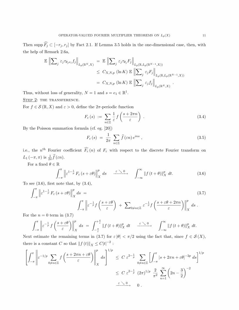
Then supp Fj ⊂ [−rj , rj ] by Fact 2.1. If Lemma 3.5 holds in the one-dimensional case, then, with

the help of Remark 2.6a,

E

∥∥∥∑jεjτθje1fj

∥∥∥Lp(RN ,X)

= E

∥∥∥∑jεjτθjFj

∥∥∥Lp(R,Lp(RN−1,X))

≤ CX,N,p (lnK) E

∥∥∥∑jεjFj

∥∥∥Lp(R,Lp(RN−1,X))

= CX,N,p (lnK) E

∥∥∥∑jεjfj

∥∥∥Lp(RN ,X)

.

Thus, without loss of generality, N = 1 and s = e1 ∈ R1.

Step 2: the transference.

For f ∈ S (R, X) and ε > 0, define the 2π-periodic function

Fε (s) :=∑n∈Z

1εf

(s+ 2πn

ε

). (3.4)

By the Poisson summation formula (cf. eg. [20])

Fε (s) =12π

∑n∈Z

f (εn) eins , (3.5)

i.e., the nth Fourier coefficient Fε (n) of Fε with respect to the discrete Fourier transform on

L1 (−π, π) is 12π f (εn).

For a fixed θ ∈ R∫ π

−π

∥∥∥ε1− 1p Fε (s+ εθ)

∥∥∥p

Xds

ε 0−−−−−→∫ ∞

−∞‖f (t+ θ)‖p

X dt. (3.6)

To see (3.6), first note that, by (3.4),∫ π

−π

∥∥∥ε1− 1p Fε (s+ εθ)

∥∥∥p

Xds = (3.7)∫ π

−π

∥∥∥∥ε− 1p f

(s+ εθ

ε

)+∑

06=n∈Zε− 1

p f

(s+ εθ + 2πn

ε

)∥∥∥∥p

X

ds .

For the n = 0 term in (3.7)∫ π

−π

∥∥∥∥ε− 1p f

(s+ εθ

ε

)∥∥∥∥p

X

ds =∫ +π

ε

−πε

‖f (t+ θ)‖pX dt

ε 0−−−−−→∫ ∞

−∞‖f (t+ θ)‖p

X dt.

Next estimate the remaining terms in (3.7) for ε |θ| < π/2 using the fact that, since f ∈ S (X),

there is a constant C so that ‖f (t)‖X ≤ C|t|−2 :∫ π

−π

∥∥∥∥∥∥ε−1/p∑

06=n∈Z

f

(s+ 2πn+ εθ

ε

)∥∥∥∥∥∥p

X

ds

1/p

≤ C ε2− 1

p

∑06=n∈Z

[∫ π

−π|s+ 2πn+ εθ|−2p ds

]1/p

≤ C ε2− 1

p (2π)1/p 2π2

∞∑n=1

(2n− 3

2

)−2

ε 0−−−−−→ 0 .


Thus (3.6) holds. Furthermore (3.6) clearly extends to linear combinations:∥∥∥∥∥∥m∑

j=1

εj ε1− 1

p (Fj)ε (· + εθj)

∥∥∥∥∥∥Lp(T,X)

ε 0−−−−−→∥∥∥∥∥∥

m∑j=1

εj fj (· + θj)

∥∥∥∥∥∥Lp(R,X)

for each choice εjmj=1 of signs ±1. Thus

E

∥∥∥∥∥∥m∑

j=1

εjε1− 1


∥∥∥∥∥∥Lp(T,X)

ε 0−−−−−→ E

∥∥∥∥∥∥m∑

j=1

εjfj (· + θj)

∥∥∥∥∥∥Lp(R,X)

. (3.8)

If supp fj ⊂ [−rj , rj ], then by (3.5), supp((Fj)ε

) ⊂ [− rj

ε ,rj

ε

]. If |θj | < K

rjand rj+1

rj≥ 2,

then, for ε small enough, there is a strictly increasing sequence njmj=1 of positive integers so

that 2nj−1 <rj

ε ≤ 2nj and thus |εθj | < Krj/ε ≤ 2K

2nj . Hence by [9, Lemma 10] applied to(Fj)ε

∈Lp (T, X) and εθj,

E

∥∥∥∥∥∥m∑

j=1

εjε1− 1


∥∥∥∥∥∥Lp(T,X)

≤ C (lnK) E

∥∥∥∥∥∥m∑

j=1

εjε1− 1

p (Fj)ε

∥∥∥∥∥∥Lp(T,X)

(3.9)

for ε small enough. Letting ε 0 in (3.8) and (3.9) finishes the proof.

Lemma 3.5 leads to the following corollary to Theorem 3.2.

Proposition 3.6. Let X be a UMD space, akk∈Z be a sequence from C with |ak| ≤ 1, and

1 < q <∞. Fix h ∈ MNN (C).

(a) Assume that supp h ⊂ t ∈ RN : b−d ≤ |t| ≤ bd

with some b > 1 and d ∈ N. Then

n (t) :=∑k∈Z

akh(b−kt

)is a Fourier multiplier on Lq

(R

N , X)

with ‖Tn‖ ≤ CX,N,q d ‖h‖MNN (C).

(b) Assume that supp h ⊂ t ∈ RN : 2−1 ≤ |t| ≤ 2

and s ∈ R

N . Then

ms (t) :=∑k∈Z

ak exp(is · 2−k t

)h(2−kt

)is a Fourier multiplier on Lq

(R

N , X)

with ‖Tms‖ ≤ CX,N,q ln (2 + |s|) ‖h‖MNN (C).

Proof. Throughout this proof, the Ci’s are constants that depend on at most: X, N , and q. To

simplify notation, let M := MNN (C). Note that h (a ·) ∈ M and ‖h (a ·)‖M = ‖h‖M for each a > 0.

Part (a) follows easily from Theorem 3.2: indeed, the support of h(b−k·) overlaps with the

support of h (b−m·) only if |m− k| < 2d; hence, n ∈ M and ‖n‖M ≤ 4d ‖h‖M.

Now to show part (b). Note that the function hs () := exp (is · ) h () is in M with ‖hs‖M ≤C1

[max

1, |s|N

]‖h‖M for some constant C1 that is independent of s. So the desired conclusion

for |s| ≤ 1 follows from part (a). Thus assume that |s| > 1.


Fix f ∈ So

(R

N , X). Then

Tmsf =∑k∈Z

ak τk(hk ∗ f)

where

Lq

(R

N , X) 3 g

τk−→ (τkg) (·) := g(· + 2−k s

)∈ Lq

(R

N , X),

and

hk (·) := h(2−k ·

),

which is a Fourier multiplier on Lq

(R

N , X)

by part (a). Thus, by the Littlewood-Paley decom-

position Corollary 3.3, for an appropriate choice of ϑ0 (eg., ϑ0 = ψ0 of Notation 3.4 so that for

then ϑkh3n+j = δk,nh3n+j),

‖Tmsf‖Lq(RN ,X) ≤1∑

j=−1

∥∥∥∥∥∑n∈Z

a3n+j τ3n+j

(h3n+j ∗ f

)∥∥∥∥∥Lq(RN ,X)

≤ C2

1∑j=−1

E

∥∥∥∥∥∑k∈Z

εk a3k+j τ3k+j

(h3k+j ∗ f

)∥∥∥∥∥Lq(RN ,X)

.

Thus, by Kahane’s contraction principle, Lemma 3.5, and then part (a),

‖Tmsf‖Lq(RN ,X) ≤ 6C2 E

∥∥∥∥∥∑k∈Z

εk τk(hk ∗ f)∥∥∥∥∥

Lq(RN ,X)

≤ C3 ln (2 |s|) E

∥∥∥∥∥∑k∈Z

εk(hk ∗ f)∥∥∥∥∥

Lq(RN ,X)

≤ C4 ln (2 + |s|) ‖h‖M ‖f‖Lq(RN ,X) .

This completes the proof of Proposition 3.6.

The logarithmic estimate in Proposition 3.6b enters the proof of the next result, which is a

centerpiece of the proof of Theorem 4.1.

Proposition 3.7. Let X have UMD and 1 < q < ∞. Let k : RN → B (X,Y ) be a strongly

integrable function such that

supp k ⊂ supp φ0 (3.10)

and∫RN

‖[k(s)]∗ g‖Lq′(RN ,X∗) w (s) ds ≤ A ‖g‖Lq′ (RN ,Y ∗) for each g ∈ Lq′(R

N , Y ∗) (3.11)

where w (·) := ln (2 + |·|). Set kj (·) := 2Njk(2j ·).

(a) For each finitely supported scalar sequence ajj∈Z with |aj | ≤ 1 and

L (·) :=∑j∈Z

ajkj (·) : RN → B (X,Y ) (3.12)


the operator

Tf := L ∗ f for f ∈ S (RN , X)

extends to a bounded operator T : Lq

(R

N , X)→ Lq

(R

N , Y)

with ‖T‖ ≤ CX,N,q A.

(b) For each f ∈ S (RN , X)

and n ∈ N

E

∥∥∥∥∥∥n∑

j=−n

εjkj ∗ f∥∥∥∥∥∥

Lq(RN ,Y )

≤ CX,N,q A ‖f‖Lq(RN ,X) . (3.13)

Also, if Y does not contain c0, then the summand in (3.13) can be taken over j ∈ Z.

Proof. Recall that the φk’s were defined in Notation 3.4.

Since k is strongly integrable, f → kj ∗ f is a bounded operator from L1

(R

N , X)

to L1

(R

N , Y).

Fix q ∈ (1,∞).

Fix f =∑m

i=1 xigi with xi ∈ X and gi ∈ S (RN ,C)

and m ∈ N. Let hj := φj−1 +φj +φj+1; note

that hj = 1 on supp φj . Put fj := hj ∗ f . Note that [kj ∗ fj ]= kj hj f = kj f = [kj ∗ f ] by (3.10).

Thus, for a.e. t ∈ RN ,

(L ∗ f) (t) =∑j∈Z

aj (kj ∗ f) (t) =∑j∈Z

aj

∫RN

2Njk(2js)fj(t− s)ds

=∫

RN

k(s)∑j∈Z

aj fj(t− 2−js)ds =∫

RN

k(s)∑j∈Z

aj (τ2−jsfj)(t)ds (3.14)

=∫

RN

k(s)(ms ∗ f)(t)ds

where τag (·) := g (· − a) and ms(t) :=∑

j aj exp(−is · 2−jt

)h0(2−jt). By Proposition 3.6

‖ms ∗ f‖Lq(RN ,X) ≤ Cw (s) ‖f‖Lq(RN ,X) (3.15)

for some constant C = CX,N,q ‖φ0‖MNN (C). If g ∈ Lq′

(R

N , Y ∗), then by (3.14), (3.15), and (3.11)∣∣〈g, L ∗ f〉Lq(Y )

∣∣ ≤∫

RN

∫RN

| 〈 g (t) , k(s) (ms ∗ f) (t) 〉Y | ds dt

≤∫

‖[k(s)]∗ g‖Lq′(X∗) ‖ms ∗ f‖Lq(X) ds ≤ C A ‖g‖Lq′(Y ∗) ‖f‖Lq(X) .

(3.16)

Thus ‖L ∗ f‖Lq(RN ,Y ) ≤ CA ‖f‖Lq(RN ,X). Hence part (a) holds.

Part (b) follows formally from part (a). Indeed, for a fixed n ∈ N and u ∈ Ω, define Lu,n (·) :=∑nj=−n εj (u) kj (·). Then by part (a)

E

∥∥∥∥∥∥n∑

j=−n

εjkj ∗ f∥∥∥∥∥∥

Lq(RN ,Y )

=∫

RN

‖Lu,n ∗ f‖Lq(RN ,Y ) du ≤ CX,N,q A ‖f‖Lq(RN ,X) . (3.17)

If Y does not contain c0, then Lq

(R

N , Y)

does not contain c0 [25] and so, by Remark 2.10c, the

sum in (3.17) can be taken over j ∈ Z. Thus part (b) holds.


Remark 3.8. a) In Proposition 3.7, if (3.11) is replaced by∫

RN ‖k(s)‖B(X,Y ) w(s)ds ≤ A, then this

modified version of Proposition 3.7 remains true.

b) In Proposition 3.7, if:

(1) in addition, Y also has UMD,

(2) in addition, the function k∗ (·) := [k (·)]∗ : RN → B (Y ∗, X∗) is strongly integrable,

(3) the condition (3.11) is replaced by:

(i)∫

RN ‖k(s)f‖Lr(Y ) w(s) ds ≤ A ‖f‖Lr(X) for each f ∈ Lr

(R

N , X)

and 1 < r ≤ 2

(ii)∫

RN ‖k∗(s)g‖Lr(X∗) w(s) ds ≤ A ‖g‖Lr(Y ∗) for each g ∈ Lr

(R

N , Y ∗) and 1 < r ≤ 2 ,

(4) CX,N,q is replaced by CX,Y,N,q,

then this modified version of Proposition 3.7 remains true (for each q ∈ (1,∞)).

Proof of Remark 3.8. a) Indeed, the calculation in (3.16) can then be replaced by

‖L ∗ f‖Lq(Y ) =∥∥∥∥∫

RN

k (s) (ms ∗ f) (·) ds∥∥∥∥

Lq(Y )

≤∫

RN

‖k (s)‖B(X,Y ) ‖ms ∗ f‖Lq(X) ds

≤ C ‖f‖Lq(X)

∫RN

‖k (s)‖B(X,Y )w (s) ds ≤ CA ‖f‖Lq(X)

with the help of (3.14) and (3.15).

b) If q ∈ [2,∞), then the modified Proposition 3.7 follows from the original Proposition 3.7 since

condition (ii) implies (3.11). So fix q ∈ (1, 2] and consider a function L of the form (3.12). Since X

and Y are UMD spaces, they are reflexive. Applying the original Proposition 3.7 to k∗ gives, by

condition (i), that

Kf := [L (·)]∗ ∗ [f (− · )] for f ∈ S (RN , Y ∗)extends to a bounded operator K : Lq′

(R

N , Y ∗)→ Lq′(R

N , X∗) with ‖K‖ ≤ CY ∗,N,q′ A. Since X

and Y are reflexive, K∗ is in B (Lq (X) , Lq (Y )) and K∗ restricted to S (RN , X)

is L (·)∗f (− · ).

In the proof of Theorem 4.1, the assumptions Remark 3.8b will be checked by applying estimates

of the operator norm of the Fourier transform on Besov spaces. The Hausdorff-Young inequality

holding in spaces with Fourier type gives a starting point for such norm estimates.

Corollary 3.9 ([14]). Let X have Fourier type p ∈ [1, 2]. Then the Fourier transform defines a

bounded operator

F : BN/pp,1

(R

N , X) −→ L1

(R

N , X). (3.18)

Furthermore, the norm of F is bounded above by a constant depending only on Fp,N (X).

A sharping of this result, in the spirit of the logarithmic estimate in Proposition 3.6, is needed in

this paper. Recall that BAp was given in Definition 2.13 and ϕkk∈N0 was given in Notation 2.11.


Corollary 3.10. Let w : RN → [0,∞) be a measurable function so that

ak := 2Nk/p ‖wχsupp ϕk‖L∞(RN ,R) < ∞ for each k ∈ N0 .

Set A := akk∈N0. If X has Fourier type p ∈ [1, 2] then the Fourier transform defines a bounded

operator

F : BAp

(R

N , X) −→ L1

((R

N , w (t) dt), X). (3.19)

Furthermore, the norm of F is bounded above by a constant depending only on Fp,N (X).

Note that if w ≡ 1 in Corollary 3.10, then (3.19) reduces to (3.18). Corollary 3.9 and Corol-

lary 3.10 remain valid if F is replaced with F−1.

Proof of Corollary 3.10. Let Jkk∈N0 be the partitioning of RN given by

Jk :=t ∈ R

N : 2k−1 < |t| ≤ 2k

for k ∈ N and J0 :=t ∈ R

N : |t| ≤ 1

and set ϕ−1 ≡ 0 and J−1 = ∅ to simplify notation.

Fix f ∈ BAp

(R

N , X). For each k ∈ N0, since ϕk ∗ f ∈ Lp

(R

N , X)

and X has Fourier type p, one

has that ϕk · f = F (ϕk ∗ f) ∈ Lp′(R

N , X); in particular, the distributional Fourier transform

of f is represented as a measurable function. Thus for each m ∈ N0

f · χJm =m∑

k=m−1

ϕk f χJm

and so (with a−1 := 0)∥∥∥f · χJm · w∥∥∥

L1(X)≤

m∑k=m−1

∥∥∥∥∥fϕk

[1 + |·|

4

]N/p

χJm

∥∥∥∥∥Lp′ (X)

∥∥∥∥∥[1 + |·|

4

]−N/p

χJmwχsupp ϕk

∥∥∥∥∥Lp(R)

≤m∑

k=m−1

∥∥∥∥∥[1 + |·|

4

]N/p

χJm

∥∥∥∥∥L∞(R)

∥∥∥fϕk

∥∥∥Lp′ (X)

‖wχsupp ϕk‖L∞(R)

∥∥∥∥∥[1 + | · |

4

]−N/p

χJm

∥∥∥∥∥Lp(R)

≤m∑

k=m−1

(2k)N/p ∥∥∥fϕk

∥∥∥Lp′ (X)

ak 2−Nk/p

[∫Jm

(1 + |t|

4

)−N

dt

]1/p

≤ Cm∑

k=m−1

ak

∥∥∥fϕk

∥∥∥Lp′ (X)

≤ C Fp,N (X)m∑

k=m−1

ak ‖ϕk ∗ f‖Lp(X)

for some universal constant C. Thus∫RN

∥∥∥f (t)∥∥∥

Xw (t) dt ≤ 2C Fp,N (X) ‖f‖BA

p (RN ,X) ,

as needed.

Let X and Y have Fourier type p and m ∈ BN/pp,1

(R

N ,B (X,Y )). Then Corollary 3.9 implies that

m ∈ L1

(R

N ,B (X,Y ))

only if p = 1 since if p > 1 then B (X,Y ) usually does not also have Fourier


type p. However, for p > 1, one can at least conclude from Corollary 3.9 that for each x ∈ X∫RN

‖ [m (·)x](t) ‖Y dt ≤ ‖F‖B

N/pp,1 (RN ,Y )→L1(RN ,Y )

‖m‖B

N/pp,1 (RN ,B(X,Y ))

‖x‖X .

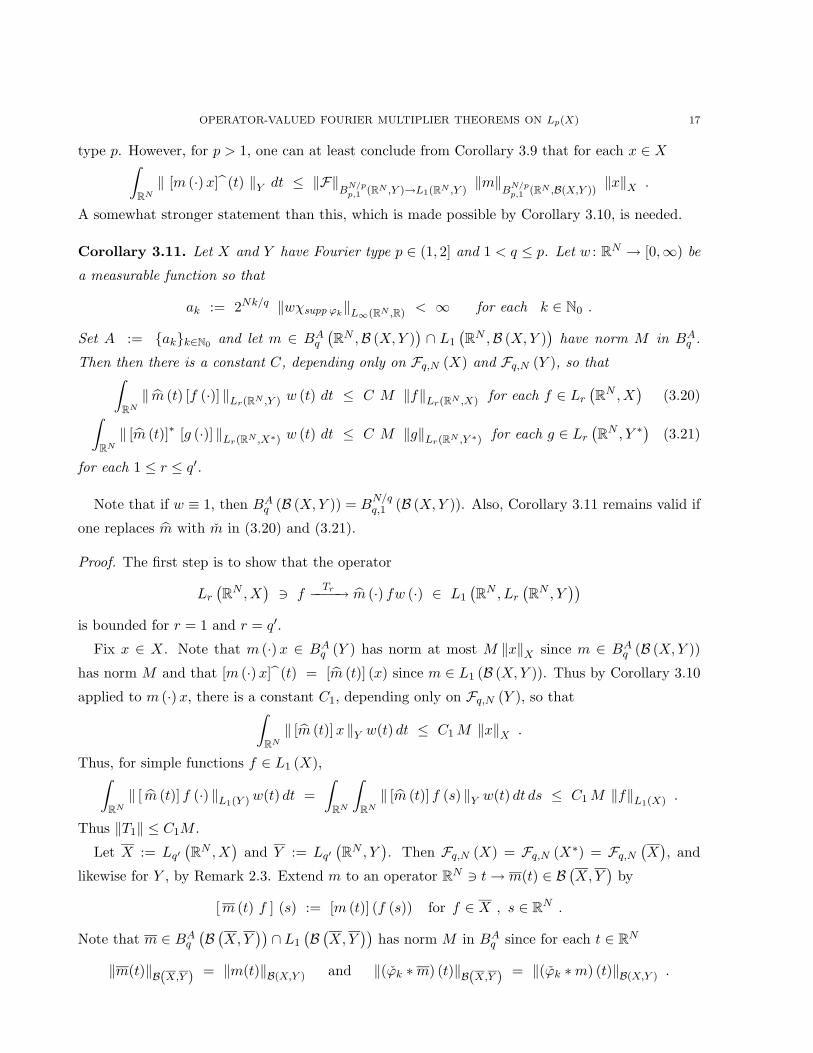
A somewhat stronger statement than this, which is made possible by Corollary 3.10, is needed.

Corollary 3.11. Let X and Y have Fourier type p ∈ (1, 2] and 1 < q ≤ p. Let w : RN → [0,∞) be

a measurable function so that

ak := 2Nk/q ‖wχsupp ϕk‖L∞(RN ,R) < ∞ for each k ∈ N0 .

Set A := akk∈N0 and let m ∈ BAq

(R

N ,B (X,Y )) ∩ L1

(R

N ,B (X,Y ))

have norm M in BAq .

Then then there is a constant C, depending only on Fq,N (X) and Fq,N (Y ), so that∫RN

‖ m (t) [f (·)] ‖Lr(RN ,Y ) w (t) dt ≤ C M ‖f‖Lr(RN ,X) for each f ∈ Lr

(R

N , X)

(3.20)∫RN

‖ [m (t)]∗ [g (·)] ‖Lr(RN ,X∗) w (t) dt ≤ C M ‖g‖Lr(RN ,Y ∗) for each g ∈ Lr

(R

N , Y ∗) (3.21)

for each 1 ≤ r ≤ q′.

Note that if w ≡ 1, then BAq (B (X,Y )) = B

N/qq,1 (B (X,Y )). Also, Corollary 3.11 remains valid if

one replaces m with m in (3.20) and (3.21).

Proof. The first step is to show that the operator

Lr

(R

N , X) 3 f

Tr−−−−→ m (·) fw (·) ∈ L1

(R

N , Lr

(R

N , Y))

is bounded for r = 1 and r = q′.

Fix x ∈ X. Note that m (·)x ∈ BAq (Y ) has norm at most M ‖x‖X since m ∈ BA

q (B (X,Y ))

has norm M and that [m (·)x](t) = [m (t)] (x) since m ∈ L1 (B (X,Y )). Thus by Corollary 3.10

applied to m (·)x, there is a constant C1, depending only on Fq,N (Y ), so that∫RN

‖ [m (t)]x ‖Y w(t) dt ≤ C1M ‖x‖X .

Thus, for simple functions f ∈ L1 (X),∫RN

‖ [ m (t)] f (·) ‖L1(Y )w(t) dt =∫

RN

∫RN

‖ [m (t)] f (s) ‖Y w(t) dt ds ≤ C1M ‖f‖L1(X) .

Thus ‖T1‖ ≤ C1M .

Let X := Lq′(R

N , X)

and Y := Lq′(R

N , Y). Then Fq,N (X) = Fq,N (X∗) = Fq,N

(X), and

likewise for Y , by Remark 2.3. Extend m to an operator RN 3 t→ m(t) ∈ B (X,Y ) by

[m (t) f ] (s) := [m (t)] (f (s)) for f ∈ X , s ∈ RN .

Note that m ∈ BAq

(B (X,Y )) ∩ L1

(B (X,Y )) has norm M in BAq since for each t ∈ R

N

‖m(t)‖B(X,Y ) = ‖m(t)‖B(X,Y ) and ‖(ϕk ∗m) (t)‖B(X,Y ) = ‖(ϕk ∗m) (t)‖B(X,Y ) .


Fix a simple function f ∈ X. Note m (·) f ∈ BAq

(Y)

has norm at most M ‖f‖X and

[m (·) f ](t) = m (t) [f (·)] .

Thus by Corollary 3.10 applied to m (·) f , there is a constant C2, depending only on Fq,N

(Y), so

that ∫RN

‖m (t) [f (·)]‖Y w (t) dt ≤ C2 M ‖f‖X .

Thus∥∥Tq′

∥∥ ≤ C2M .

Thus (3.20) holds for 1 ≤ r ≤ q′ by interpolation in the scale of Bochner-spaces (see [6,

Thm. 5.1.2]). Claim (3.21) is obtained by applying the same argument to [m(t)]∗ ∈ B (Y ∗, X∗).

One more preparatory result is needed for the proof of Theorem 4.1. The proof of the following

lemma is due to N.J. Kalton and replaces our original (more complicated) proof. Recall that εkk∈Z

and ε′kk∈Z were given in Notation 2.7.

Lemma 3.12. For any Banach space X and any array xklk,l∈Z from X

E ε

∥∥∥∥∥∑k∈Z

εkxkk

∥∥∥∥∥X

≤ E ε,ε′

∥∥∥∥∥∥∑k,l∈Z

εkε′lxkl

∥∥∥∥∥∥X

.

Proof. For αk ∈ −1, 1, the sequences of random variables εk, ε′k, αk εk, and αk ε′k have

the same distribution. Hence by Fubini’s theorem

E ε,ε′

∥∥∥∥∥∥∑k,l∈Z

εkε′lxkl

∥∥∥∥∥∥X

= E ε,ε′

∥∥∥∥∥∥∑k,l∈Z

αk αl εkε′lxkl

∥∥∥∥∥∥X

. (3.22)

Let ηk be a sequence of −1,+1–valued, independent, symmetric random variables that is

independent of εk and ε′k. Integrating (3.22) gives

E ε,ε′

∥∥∥∥∥∥∑k,l∈Z

εkε′lxkl

∥∥∥∥∥∥X

= E ε,ε′ E η

∥∥∥∥∥∥∑k,l∈Z

ηkηlεkε′lxkl

∥∥∥∥∥∥X

≥ E ε,ε′

∥∥∥∥∥∥E η

∑k,l∈Z

ηkηlεkε′lxkl

∥∥∥∥∥∥X

= E ε,ε′

∥∥∥∥∥∑k∈Z

εkε′kxkk

∥∥∥∥∥X

= E ε

∥∥∥∥∥∑k∈Z

εkxkk

∥∥∥∥∥X

,

again since u→ εk (u) · ε′k (v), for each fixed v, is a sequence of independent random variables with

the same distribution as εk.

4. FOURIER MULTIPLIER THEOREMS

This section explores operator-valued Fourier multiplier operators. The assumptions of the main

result, Theorem 4.1, may be somewhat awkward looking. However, with respect to the smoothness

of the multiplier function, it is a rather weak assumption that will make it easy to derive, in a


unified way, several results modeled after classical conditions, such as of Mihlin and Hormander,

as shown by the corollaries to follow.

Theorem 4.1. Let X and Y be UMD spaces with Fourier type p ∈ (1, 2] and 1 < q < ∞. Set

X := Radq (X) and Y := Radq (Y ). Let m : RN \ 0 → B (X,Y ) be a measurable function that

induces a mapping M : RN → B

(X, Y

),

M(s) :=φ0(s)m(2ks)

k∈Z

for s 6= 0 and M(0) := 0 ,

that satisfies M ∈ BAp

(R

N ,B(X, Y

))with norm D where A =

(k ∨ 1) 2Nk/p

k∈N0

. Then m

is a Fourier multiplier from Lq(RN , X) to Lq(RN , Y ). Furthermore, ‖Tm‖Lq→Lq≤ C D for some

constant C depending on: X, Y , N , p, q, and φ0.

Remark 4.2. a) Recall that each UMD space has Fourier type p for some p > 1.

b) Remark 2.10 provides a convenient way to compute the norm of M ; indeed, ‖M (s)‖B(X,Y ) =

φ0(s)Rq

(m(2ks) : k ∈ Z

)for each s ∈ R

N .

c) For the A in Theorem 4.1, there are continuous embeddings

W lp

(R

N , Z) ⊂ Bs

p,r

(R

N , Z) ⊂ BA

p

(R

N , Z) ⊂ B

N/pp,1

(R

N , Z)

where N/p < s < l ∈ N and r ∈ [1,∞].

d) The exponent N/p is best possible in the following sense. Let Ap :=(k ∨ 1) 2Nk/p

k∈N0

. Note

that the spaces BApp form a scale since, for 1 ≤ p < q <∞,

BApp

(R

N , Z) ⊂ B

Aqq

(R

N , Z).

In general it is not possible to replace BApp in Theorem 4.1 by a larger space BAq

q for some q > p.

This follows as in [14, Remark 4.9].

Proof of Theorem 4.1. Throughout this proof, the Ci’s denotes constants which depend on at most:

X, Y , N , p, q, and φ0. Note that X and Y are UMD spaces with Fourier type p by Remark 2.10.

Since M ∈ L∞(R

N ,B(X, Y

))has bounded support, M ∈ L1

(R

N ,B(X, Y

)). Define the

function K by:

RN 3 s → K(s) :=

(F−1M)(s) ∈ B

(X, Y

).

Corollary 3.11 applied to M ∈ BAp

(B(X, Y

))with w(t) = ln (2 + |t|) gives that for 1 ≤ r ≤ 2∫

RN

‖K(t)F (·)‖Lr(Y ) w (t) dt ≤ C1D ‖F‖

Lr(X) for each F ∈ Lr

(X)

∫RN

‖[K(t)]∗G (·)‖Lr(X∗) w (t) dt ≤ C1D ‖G‖

Lr(Y ∗) for each G ∈ Lr

(Y ∗).


Also, K and K∗ are strongly integrable by Corollary 3.9 and supp K ⊂ supp φ0. Thus Remark 3.8b

can be applied to K ∈ L∞(B(X, Y

)). Hence for Kj (·) := 2NjK

(2j · ), condition (3.13) gives

that for each F ∈ S(R

N , X)

E

∥∥∥∥∥∥∑j∈Z

εjKj ∗ F∥∥∥∥∥∥

Lq(Y )

≤ C2C1D ‖F‖Lq(X) . (4.1)

To see that inequality (4.1) implies the boundedness of Tm, fix f ∈ So (X) and let hk := φk−1 +

φk + φk+1. Then F :=hk ∗ f

k∈Z∈ S

(X)

and by Corollary 3.3

‖F‖Lq(X) ≤

1∑j=−1

∥∥∥φk+j ∗ f

k∈Z

∥∥∥Lq(X)

= 3∥∥∥φk ∗ f

k∈Z

∥∥∥Lq(X)

≤ C3 ‖f‖Lq(X) . (4.2)

Note that M ∈ L∞ implies that m ∈ L∞; thus it follows from Remark 3.8b that

Kj ∗ F =φj ∗ hk ∗ Tm(2k−j ·)f

k∈Z

∈ Lq

(Y)

= Radq (Lq (Y ))

since, for a.e. s,

(Kj ∗ F )(s) = M(2−js

)F (s) =

φ0

(2−js

)m(2k−js

)hk (s) f (s)

k∈Z

=φj (s)hk (s)

(Tm(2k−j ·)f

)(s)

k∈Z

.

Since hk is 1 on the support of φk, if j = k then φj ∗ hk ∗ Tm(2k−j ·) (f) = φj ∗ (Tmf). Hence, by

Corollary 3.3 and Lemma 3.12,

‖Tmf‖Lq(Y ) ≤ C4 E ε

∥∥∥∥∥∥∑j∈Z

εj φj ∗ Tmf

∥∥∥∥∥∥Lq(Y )

≤ C4 E ε,ε′

∥∥∥∥∥∥∑k∈Z

ε′k

∑j∈Z

εjφj ∗ hk ∗ Tm(2k−j ·)f

∥∥∥∥∥∥Lq(Y )

(4.3)

= C4 E ε

∥∥∥∥∥∥∑

j∈Z

εjφj ∗ hk ∗ Tm(2k−j ·)f

k∈Z

∥∥∥∥∥∥Rad1(Lq(Y ))

≤ C5 E ε

∥∥∥∥∥∥∑j∈Z

εj

φj ∗ hk ∗ Tm(2k−j ·)f

k∈Z

∥∥∥∥∥∥Lq(Y )

= C5 E ε

∥∥∥∥∥∥∑j∈Z

εjKj ∗ F∥∥∥∥∥∥

Lq(Y )

.

Combining (4.1), (4.2), and (4.3) gives that ‖Tmf‖Lq(Y ) ≤ C6D ‖f‖Lq(X).

The following notation simplifies the statements of corollaries to come.

Notation 4.3. Let RMNl (B (X,Y )) be the set of all measurable functionsm : R

N \ 0 → B (X,Y )

whose distributional derivatives Dαm are represented by measurable functions for each α ∈ NN0


with |α| ≤ l and

‖m‖RMNl (B(X,Y )) := max

α∈NN0

|α|≤l

R2

(|t||α|Dαm (t) : t ∈ R

N \ 0)

< ∞ (4.4)

where l ∈ N0.

Note that if X and Y are Hilbert spaces, then ‖m‖MNl (B(X,Y )) = ‖m‖RMN

l (B(X,Y )).

The following Mihlin-type multiplier theorem is an immediate consequence of Theorem 4.1.

Corollary 4.4. Let X and Y be UMD spaces with Fourier type p ∈ (1, 2] and l :=[

Np

]+ 1. If

m ∈ RMNl (B (X,Y )) with ‖m‖RMN

l (B(X,Y )) := A

then m is a Fourier multiplier from Lq(RN , X) to Lq(RN , Y ) for each q ∈ (1,∞). Furthermore,

‖Tm‖Lq→Lq≤ C A for some constant C independent of m.

Remark 4.5. a) Corollary 4.4 applies to Hilbert spaces X and Y with l = [N/2]+1, which recovers

Schwartz’s classical result. For arbitrary UMD spaces, Corollary 4.4, but with l = N , was first

shown in [35], for a second proof see [16]. Furthermore, [36, Remark 3.7] shows that the expo-

nent l := [N/p] + 1 is best possible for Lp-spaces.

b) The proof will show that the assumption (4.4) on m can be replaced by the following formally

weaker assumption:

maxα∈NN

0|α|≤l

supt∈RN

2−1≤|t|≤21

R2

(∣∣∣2kt∣∣∣|α|Dαm(2kt) : k ∈ Z

):= A <∞ . (4.5)

Proof of Corollary 4.4. Let B := B (Radq (X) ,Radq (Y )). Without loss of generality, via an ap-

proximation argument, suppm ⊂ t ∈ R

N : 2−n ≤ |t| ≤ 2n

for some n ∈ N. Thus, if s ∈ RN

then M (s) :=φ0 (s)m(2ks)

k∈Z

∈ B with the kth coordinate of M (s) being zero for |k| > n. By

Leibniz’s rule and Remark 2.10a,

‖M‖W lp(RN ,B) ≤

∑|α|≤l

2|α|∥∥∥|t||α|DαM (t) χsupp φ0 (t)

∥∥∥Lp(dt,B)

≤∑|α|≤l

∑β≤α

2|α|(α

β

)∥∥∥∥|t||α−β|Dα−βφ0 (t)∣∣∣2kt

∣∣∣|β|Dβm(2kt)

k∈Z

∥∥∥∥Lp(dt,B)

=∑|α|≤l

∑β≤α

2|α|(α

β

)∥∥∥∥|t||α−β|Dα−βφ0 (t) Rq

(∣∣∣2kt∣∣∣|β|Dβm

(2kt)

: k ∈ Z

)χ[2−1≤|t|≤2]

∥∥∥∥Lp(dt,R)

.

By (4.5) and Holder’s inequality, M ∈W lp

(R

N , B). By Remark 4.2c, Theorem 4.1 applies.


Np

]+ 1. Let

m ∈ RMNl (B (X,Y )) and set ‖m‖RMN

l (B(X,Y )) := A.

(a) Then m is a Fourier multiplier from H1

(R

N , X)

to L1

(R

N , Y)

and ‖Tm‖H1→L1≤ C A for


some constant C independent of m.

(b) Then m is a Fourier multiplier from L1

(R

N , X)

to Lwk1

(R

N , Y)

and ‖Tm‖L1→Lwk1

≤ C A for

some constant C independent of m.

(c) Then m is a Fourier multiplier from L∞(R

N , X)

to BMO(R

N , Y)

and ‖Tm‖L∞→BMO ≤ C A

for some constant C independent of m.

Remark 4.7. A related result, which also covers the spaces Hp for p < 1 was found independently

by T. Hytonen [18].

A word about what is meant by a Fourier multiplier for UMD spaces X and Y for the function

spaces in Corollary 4.6 is in order. Since SH

(R

N , X)

:=f ∈ S (RN , X

):∫

RN f (t) dt = 0

is

norm-dense in H1

(R

N , X), it is clear what is meant by a Fourier multiplier from H1 to L1: in

Definition 2.4, just replace S by SH and Lq by either H1 or L1, accordingly. A linear mapping

T : L1

(R

N , X)→ Lwk

1

(R

N , Y)

is (uniformly) continuous if and only if

‖T‖L1→Lwk1

:= sup‖Tf‖Lwk

1: ‖f‖L1

≤ 1< ∞ .

If a linear mapping T : S (RN , X)→ Lwk

1

(R

N , Y)

satisfies

‖Tf‖Lwk1 (RN ,Y ) ≤ C ‖f‖L1(RN ,X) for each f ∈ S (RN , X

),

then, since S (RN , X)

is a norm-dense subspace of L1

(R

N , X), there is a unique continuous linear

extension T : L1

(R

N , X) → Lwk

1

(R

N , Y)

of T and ‖T‖L1→Lwk1

≤ 2C. Thus it is clear what

is meant by a Fourier multiplier from L1 to Lwk1 : in Definition 2.4, just replace Lq by either L1

or Lwk1 , accordingly. The Schwartz class is not norm-dense in L∞; however, it is weak∗-dense in L∞.

Since X and Y are UMD spaces (in particular, reflexive)

[H1

(R

N , Y ∗)]∗ = BMO(R

N , Y)

and[L1

(R

N , Y ∗)]∗ = L∞(R

N , Y),

(cf. [9] for H1–BMO duality). Thus m is a Fourier multiplier from L∞(R

N , X)

to BMO(R

N , Y)

provided there is an operator Tm ∈ B (L∞(R

N , X), BMO

(R

N , Y))

satisfying:

Tmf :=[mf

]∨for each f ∈ S (RN , X

)Tm is weak∗-to-weak∗ continuous .

(4.6)

Note that (4.6) guarantees the uniqueness of a norm-to-norm continuous operator, if it exists.

Proof of Corollary 4.6. Throughout this proof, the Ci’s are constants that are independent of m

and the fixed n ∈ N.


For each j ∈ Z and a fixed n ∈ N, let

mj := mφj Mn :=n∑

j=−∞mj

kj := mj Kn := Mn =n∑

j=−∞kj .

Note that Mn ∈ RMNl (B (X,Y )) with

‖Mn‖RMNl (B(X,Y )) ≤ C0A .

So TMn ∈ B (L2

(R

N , X), L2

(R

N , Y))

by Corollary 4.4. That TMn satisfies parts (a) and (b), for

some constant C independent ofm and the fixed n ∈ N, follows from the Benedek-Calderon-Panzone

theorem for convolutions on vector-valued spaces (see [13, Ch. V, Thm 3.4 and Remark (3.3′) on

p. 494]) if one can show that∫|t|>2|s|

‖Kn (t− s)x−Kn (t)x‖Y dt ≤ AC1 ‖x‖X (4.7)

for each s ∈ RN and x ∈ X. Inequality (4.7) is now shown via an adaption of the classical argument

in [32, Ch. VI, Sect. 4.4].

Fix x ∈ X. For α ∈ NN0 with |α| ≤ l, by Leibniz’s rule,

‖Dαmj (t)‖B(X,Y ) ≤ AC32−j|α| ;

thus, since (Dαmj)∨ (t) = (−it)α kj (t) and Y has Fourier type p,[∫

RN

‖(−it)α kj (t)x‖p′Y dt

]1/p′

≤ C4

[∫supp φj

‖Dαmj (t)x‖pY dt

]1/p

≤ AC5 2−j|α| 2jNp ‖x‖X .

Thus for each l0 ∈ 0, 1, . . . , l[∫RN

∥∥∥|t|l0 kj (t)x∥∥∥p′

Ydt

]1/p′

≤ AC6 2jNp 2−jl0 ‖x‖X . (4.8)

Using (4.8) with l = l0, Holder’s inequality gives, for any a > 0, since N/p < l,∫|t|≥a

‖kj (t)x‖Y dt ≤[∫

RN

∥∥∥|t|l kj (t)x∥∥∥p′

Ydt

]1/p′[∫

|t|≥a|t|−lp dt

]1/p

≤ AC6 2jNp 2−jl ‖x‖X a

Np a−l

[∫|t|≥1

|t|−lp dt

]1/p

≤ AC7

(2ja)N

p−l ‖x‖X .

(4.9)

Similarly, taking l0 = 0 in (4.8) gives∫|t|≤a

‖kj (t)x‖Y dt ≤[∫

RN

‖kj (t)x‖p′Y dt

]1/p′[∫

|t|≤a1 dt

]1/p

≤ AC8

(2ja)N

p ‖x‖X . (4.10)


Choosing a = 2−j in (4.9) and (4.10) gives∫RN

‖kj (t)x‖Y dt ≤ AC9 ‖x‖X .

Let nj (t) := [Dαkj ](t) = (i)|α| tαmj (t) for each j ∈ Z. For β ∈ NN0 with |β| ≤ l∥∥∥Dβnj (t)

∥∥∥B(X,Y )

≤ AC10 2j|α| 2−j|β|

by Leibniz’s rule; thus, since[Dβnj

]∨ (t) = (−i)|β| tβ Dαkj (t) and Y has Fourier type p,[∫RN

∥∥∥tβDαkj (t)x∥∥∥p′

Ydt

]1/p′

≤ C11

[∫RN

∥∥∥Dβnj (t)x∥∥∥p

Ydt

]1/p

≤ AC12 2j|α| 2−j|β|2jN/p .

Arguing as above gives that∫RN

‖Dαkj (t)x‖Y dt ≤ AC132j|α| ‖x‖X . (4.11)

Thus, for each h = (h1, . . . , hN ) ∈ RN ,∫

RN

‖kj (t+ h)x− kj (t)x‖Y dt ≤∫ 1

0

(N∑

i=1

|hi|∫

RN

∥∥∥∥ ∂∂tikj (t+ sh)x∥∥∥∥

Y

dt

)ds

≤ AC14 2j |h| ‖x‖X ;

(4.12)

indeed, just apply the Fundamental Theorem of Calculus to Rn 3 s → kj (t+ sh)x ∈ Y and then

use (4.11). Fix s ∈ RN . Note that the inequality∑j∈Z

∫|t|>2|s|

‖kj (t− s)x− kj (t)x‖Y dt ≤ AC15 ‖x‖X (4.13)

implies (4.7). To see (4.13), let Γ1 :=j ∈ N : 2j ≤ |s|−1

and Γ2 :=

j ∈ N : |s|−1 < 2j

.

By (4.12),∑j∈Γ1

∫|t|>2|s|

‖kj (t− s)x− kj (t)x‖Y dt ≤ AC14 ‖x‖X

[|s|∑

j∈Γ1

2j]

≤ AC16 ‖x‖X .

By (4.9)∑j∈Γ2

∫|t|>2|s|

‖kj (t− s)x− kj (t)x‖Y dt ≤ 2∑j∈Γ2

∫|t|>1 |s|

‖kj (t)x‖Y dt

≤ 2 AC7 ‖x‖X

[|s|N

p−l∑

j∈Γ2

(2

Np−l)j]

≤ AC17 ‖x‖X

since N/p < l. This completes the proof of (4.7). Thus TMn satisfies parts (a) and (b) for some

constant C18 independent of m and n ∈ N.

Towards showing part (a), fix f ∈ SH

(R

N , X)

and let

G :=g ∈ S (RN , Y ∗) : ‖g‖L∞(Y ∗) ≤ 1

.


Then

‖Tmf‖L1(RN ,Y ) = supg∈G

〈g, Tmf〉 = supg∈G

limn→∞ 〈g, TMnf〉 ≤ sup

g∈Glim

n→∞‖g‖L∞(Y ∗) ‖TMnf‖L1(Y )

≤ limn→∞

‖TMn‖H1(X)→L1(Y ) ‖f‖H1(X) ≤ AC18 ‖f‖H1(X) .

Thus part (a) holds.

If f ∈ S∗(R

N , X)

:=g ∈ S (RN , X

): supp g is compact

, then Tmf = TMnf for n sufficiently

large. Since S∗(R

N , X)

is norm-dense in L1

(R

N , X), part (b) holds.

Part (c) follows from part (a) and a duality argument. Since X and Y have nontrivial (Fourier)

type, m∗ ∈ RMNl (B (Y ∗, X∗)) and ‖m∗‖RMN

l (B(Y ∗,X∗)) ≤ C19 ‖m‖RMNl (B(X,Y )) (cf., eg., [39,

Thm. 2.2.14]). Thus Tm∗ ∈ B (H1

(R

N , Y ∗) , L1

(R

N , X∗)) with ‖Tm∗‖H1→L1≤ AC20 by part (a).

Hence (Tm∗)∗ ∈ B (L∞(R

N , X), BMO

(R

N , Y))

is weak∗-to-weak∗ continuous and is of norm at

most AC20. Furthermore, (Tm∗)∗ |S(RN ,X) = Tm(−·) |S(RN ,X) . Thus part (c) holds.

Remark 4.8. One can use the estimates in the proof of Corollary 4.6 to give a more direct proof

of Corollary 4.4 avoiding Besov spaces. We indicate this for p = 1, l = [N ] + 1: By assumption

M(t) = (φ0(t)m(2kt)) andM (α), where |α| ≤ N+1, have norm less than C in B (Rad (X) ,Rad (Y )).

Estimates (4.9) and (4.10) applied to K(t) = M(t)∨ with p = 1 give∫

RN ‖k(t)‖ dt < ∞ for the

operator norm on B (Rad (X) ,Rad (Y )). Now apply Remark 3.8a and finish the proof as in the

last part of the proof of Theorem 4.1.

Our results are easily adapted to Sobolev spaces. Corollary 4.9 gives a flavor of this for fractional

Sobolev spaces (see Definition 2.15).

Corollary 4.9. Let X and Y have UMD and Fourier type p ∈ (1, 2] and l :=[

Np

]+ 1 and s ∈ R.

Assume that m ∈ Cl(R

N \ 0 ,B (X,Y ))

satisfies that

maxα∈NN

0|α| ≤ l

R2

( (1 + |t|2)s/2 |t||α| (Dαm) (t) : t ∈ R

N \ 0 )

:= A ≤ ∞ . (4.14)

Then m is a Fourier multiplier from Hrq

(R

N , X)

to Hr+sq

(R

N , Y)

for each r ∈ R and q ∈ (1,∞).

Also, ‖Tm‖Hrq→Hr+s

q≤ C A for some constant C independent of m.

Proof. It suffices to show that n (·) :=(1 + |·|2

)s/2m (·) is a Fourier multiplier from Lq

(R

N , X)

to Lq

(R

N , Y); for then, the following diagram

Hrq

(R

N , X) Tm−−−−→ Hr+s

q

(R

N , Y)

Jr

y yJr+s

Lq

(R

N , X) Tn−−−−→ Lq

(R

N , Y)


commutes, where Ju : Huq

(R

N , Z)→ Lq

(R

N , Z)

is the isometry defined by

Ju (f) :=[(

1 + |·|2)u/2

f (·)]∨

for f ∈ S (RN , Z).

But

|t||α| Dαn (t) = |t||α| Dα

[(1 + |·|2

)s/2m (·)

](t)

=∑β≤α

(α

β

)|t||β|Dβ

[(1 + |·|2

)s/2]

(t)(1 + |t|2

)s/2

[(

1 + |t|2)s/2 |t||α−β| Dα−βm (t)

](4.15)

and the terms · · · in (4.15) are uniformly bounded on RN \ 0. Thus the assumption (4.14)

gives that n ∈ RMNl (B (X,Y )) and so Corollary 4.4 finishes off the proof.

Hormander’s condition takes here the following form.


Np

]+ 1.

Let m : RN \ 0 → B (X,Y ) be a measurable function whose distributional derivatives Dαm are

represented by measurable functions for each α ∈ NN0 with |α| ≤ l and

maxα∈NN

0|α| ≤ l

∫2−1<|t|<2

[R2

( ∣∣∣2kt∣∣∣|α|Dαm

(2kt)

: k ∈ Z

) ]p

dt := A < ∞ . (4.16)

Then m is a Fourier multiplier from Lq(X) to Lq(Y ) for each 1 < q <∞. Also, ‖Tm‖Lq→Lq≤ CA

for some constant C independent of m.

Proof. In the proof of Corollary 4.4, just replace (4.5) by (4.16) to see that Theorem 4.1 applies in

this setting also.

The following corollary shows that our result improves on the multiplier theorem of Bourgain

even in the case of scalar-valued multiplier functions m. Its proof uses the following equivalent

norm [29, Prop. 3.1] on the Besov spaces Bsp,1 (R, Z) for 0 < s < 1 and 1 ≤ p <∞:

‖f‖′Bsp,1(R,Z) := ‖f‖Lp(R,Z) + Bs

p,1 (f)

where fh (u) := f (u+ h),

Bsp,1 (f) :=

∫ ∞

0t−swp (f, t)

dt

t

wp (f, t) := sup|h|≤t

‖fh − f‖Lp(R,Z) .


Corollary 4.11. Let X and Y be UMD spaces with Fourier type p ∈ (1, 2]. Assume that for the

function m : R \ 0 → B (X,Y ) there is some l ∈(

1p , 1)

and h0 > 0 so that, for some constant A,

R2 (m (u) : u ∈ R \ 0) ≤ A

R2

(|u|l m (u+ h) − m (u)

|h|l : u, u+ h ∈ R \ 0 and 0 < |h| ≤ |u| h0

)≤ A .

(4.17)

Then m is a Fourier multiplier from Lq (R, X) to Lq (R, Y ) for each q ∈ (1,∞). Furthermore,

‖Tm‖Lq→Lq≤ C A for some constant C independent of m.

Proof. Throughout this proof, the Cj ’s are constants independent of m. Without loss of general-

ity, h0 <14 . Fix s so that 0 < 1

p < s < l < 1.

Set m (0) := 0. For t ∈ R, let mk(t) := φ0(t)m(2kt) and M (t) := mk (t)k∈Z. Note that∣∣∣u

h

∣∣∣l [mk(u+ h) −mk(u)] =

φ0(u)∣∣∣uh

∣∣∣l [m(2k (u+ h))−m

(2ku)]

+ m(2k (u+ h)

) ∣∣∣uh

∣∣∣l [φ0 (u+ h) − φ0 (u)] .

So, since φ0 ∈ S and l < 1, the assumption (4.17) yields, for each u, h ∈ R\0 with 0 < |h| ≤ |u|h0,

R2 (mk (u+ h) −mk (u) : k ∈ Z) ≡∣∣∣∣hu∣∣∣∣l R2

(∣∣∣uh

∣∣∣l [mk (u+ h) −mk (u)] : k ∈ Z

)≤∣∣∣∣hu∣∣∣∣l AC1 .

Thus, if |h| ≤ h04 then, with B := B (Radq (X) ,Radq (Y )),

‖Mh −M‖Lp(B) =

[∫ 3

14

‖M (u+ h) −M (u)‖pB du

] 1p

≤ AC2

[∫ 3

14

∣∣∣∣hu∣∣∣∣lp du

] 1p

≤ AC3 |h|l

since 1p < l. Also, ‖Mh −M‖Lp(B) ≤ 2 ‖M‖Lp(B) ≤ AC4 for any h ∈ R. Thus

wp (M, t) ≤AC5 t

l if t ≤ h04

AC6 if t > h04 .

Thus Bsp,1 (M) ≤ AC8 since 0 < s < l and so M ∈ Bs

p,1 (R, B) with norm at most AC9. By

Remark 4.2c, since 1p < s, we can apply Theorem 4.1, one last time.

References

[1] Herbert Amann, Linear and quasilinear parabolic problems. Vol. I, Birkhauser Boston Inc., Boston, MA, 1995,Abstract linear theory. MR 96g:34088

[2] , Operator-valued Fourier multipliers, vector-valued Besov spaces, and applications, Math. Nachr. 186(1997), 5–56. MR 98h:46033

[3] , Elliptic operators with infinite-dimensional state spaces, J. Evol. Equ. 1 (2001), no. 2, 143–188. MR 1846 745

[4] Wolfgang Arendt and Shangquan Bu, The operator-valued Marcinkiewicz multiplier theorem and maximal regu-larity, Math. Z. 240 (2002), no. 2, 311–343. MR 1 900 314

[5] A. Benedek, A.-P. Calderon, and R. Panzone, Convolution operators on Banach space valued functions, Proc.Nat. Acad. Sci. U.S.A. 48 (1962), 356–365. MR 24 #A3479


[6] Joran Bergh and Jorgen Lofstrom, Interpolation spaces. An introduction, Springer-Verlag, Berlin, 1976,Grundlehren der Mathematischen Wissenschaften, No. 223. MR 58 #2349

[7] Sonke Blunck, Maximal regularity of discrete and continuous time evolution equations, Studia Math. 146 (2001),no. 2, 157–176. MR 1 853 519

[8] J. Bourgain, A Hausdorff-Young inequality for B-convex Banach spaces, Pacific J. Math. 101 (1982), no. 2,255–262. MR 84d:46014

[9] , Vector-valued singular integrals and the H1-BMO duality, Probability theory and harmonic analysis(Cleveland, Ohio, 1983), Dekker, New York, 1986, pp. 1–19. MR 87j:42049b

[10] , Vector-valued Hausdorff-Young inequalities and applications, Geometric aspects of functional analysis(1986/87), Springer, Berlin, 1988, pp. 239–249. MR 89m:46069

[11] Philippe Clement and Jan Pruss, An operator-valued transference principle and maximal regularity on vector-valued Lp-spaces, Evolution equations and their applications in physical and life sciences (Bad Herrenalb, 1998)(Gunter Lummer and Lutz Weis, eds.), Dekker, New York, 2001, pp. 67–87. MR 2001m:47064

[12] Joe Diestel, Hans Jarchow, and Andrew Tonge, Absolutely summing operators, Cambridge University Press,Cambridge, 1995. MR 96i:46001

[13] Jose Garcıa-Cuerva and Jose L. Rubio de Francia, Weighted norm inequalities and related topics, North-HollandPublishing Co., Amsterdam, 1985, Notas de Matematica [Mathematical Notes], 104. MR 87d:42023

[14] Maria Girardi and Lutz Weis, Operator-valued Fourier multiplier theorems on Besov spaces, MathematischeNachrichten, (to appear).

[15] , Vector-valued extentions of some classical theorems in harmonic analysis, Analysis and Applications -ISAAC 2001 (H. G. W. Begehr, R. P. Gilbert, and M. W. Wong, eds.), Kluwer, Dordrecht, (to appear).

[16] Robert Haller, Horst Heck, and Andre Noll, Mikhlin’s theorem for operator-valued Fourier multipliers in nvariables, Math. Nachr. 244 (2002), 110–130. MR 1 928 920

[17] Matthias Hieber, A characterization of the growth bound of a semigroup via Fourier multipliers, Evolutionequations and their applications in physical and life sciences (Bad Herrenalb, 1998) (Gunter Lummer and LutzWeis, eds.), Dekker, New York, 2001, pp. 121–124. MR 2002a:47064

[18] Tuomas Hytonen, Convolutions, multipliers, and maximal regularity on vector-valued Hardy spaces, HelsinkiUniversity of Technology Institute of Mathematics Research Reports (preprint).

[19] Tuomas Hytonen and Lutz Weis, Singular convolution integrals with operator-valued kernels, (submitted).[20] Frank Jones, Lebesgue integration on Euclidean space, Jones and Bartlett Publishers, Boston, MA, 1993. MR

93m:28001[21] N. J. Kalton and L. Weis, The H∞-calculus and sums of closed operators, Math. Ann. 321 (2001), no. 2, 319–345.

MR 1 866 491[22] Hermann Konig, On the Fourier-coefficients of vector-valued functions, Math. Nachr. 152 (1991), 215–227. MR

92m:46049[23] P. C. Kunstmann, Maximal Lp-regularity for second order elliptic operators with uniformly continuous coefficients

on domains, (submitted).[24] S. Kwapien, Isomorphic characterizations of inner product spaces by orthogonal series with vector valued coeffi-

cients, Studia Math. 44 (1972), 583–595, Collection of articles honoring the completion by Antoni Zygmund of50 years of scientific activity, VI. MR 49 #5789

[25] , On Banach spaces containing c0, Studia Math. 52 (1974), 187–188, A supplement to the paper by J.Hoffmann-Jørgensen: “Sums of independent Banach space valued random variables” (Studia Math. 52 (1974),159–186). MR 50 #8627

[26] Y. Latushkin and F. Rabiger, Fourier multipliers in stability and control theory, (preprint).[27] Terry R. McConnell, On Fourier multiplier transformations of Banach-valued functions, Trans. Amer. Math.

Soc. 285 (1984), no. 2, 739–757. MR 87a:42033[28] Jaak Peetre, Sur la transformation de Fourier des fonctions a valeurs vectorielles, Rend. Sem. Mat. Univ. Padova

42 (1969), 15–26. MR 41 #812[29] A. Pe lczynski and M. Wojciechowski, Molecular decompositions and embedding theorems for vector-valued Sobolev

spaces with gradient norm, Studia Math. 107 (1993), no. 1, 61–100. MR 94h:46050[30] Hans-Jurgen Schmeisser, Vector-valued Sobolev and Besov spaces, Seminar analysis of the Karl-Weierstraß-

Institute of Mathematics 1985/86 (Berlin, 1985/86), Teubner, Leipzig, 1987, pp. 4–44. MR 89h:46053[31] Bert-Wolfgang Schulze, Boundary value problems and singular pseudo-differential operators, John Wiley & Sons

Ltd., Chichester, 1998. MR 99m:35281[32] Elias M. Stein, Harmonic analysis: real-variable methods, orthogonality, and oscillatory integrals, Princeton

University Press, Princeton, NJ, 1993, With the assistance of Timothy S. Murphy, Monographs in HarmonicAnalysis, III. MR 95c:42002


[33] Elias M. Stein and Guido Weiss, Introduction to Fourier analysis on Euclidean spaces, Princeton UniversityPress, Princeton, N.J., 1971, Princeton Mathematical Series, No. 32. MR 46 #4102

[34] Hans Triebel, Fractals and spectra, Birkhauser Verlag, Basel, 1997, Related to Fourier analysis and functionspaces. MR 99b:46048

[35] Z. Strkalj and Lutz Weis, On operator-valued Fourier multiplier theorems, (submitted).[36] Lutz Weis, Stability theorems for semi-groups via multiplier theorems, Differential equations, asymptotic analysis,

and mathematical physics (Potsdam, 1996), Akademie Verlag, Berlin, 1997, pp. 407–411. MR 98h:47062[37] , A new approach to maximal Lp-regularity, Evolution equations and their applications in physical and

life sciences (Bad Herrenalb, 1998) (Gunter Lummer and Lutz Weis, eds.), Dekker, New York, 2001, pp. 195–214.MR 2002a:47068

[38] , Operator-valued Fourier multiplier theorems and maximal Lp-regularity, Math. Ann. 319 (2001), no. 4,735–758. MR 2002c:42016

[39] H. Witvliet, Unconditional schauder decompositions and multiplier theorems, Ph.D. thesis, Technische Univer-siteit Delft, November 2000.

[40] Frank Zimmermann, On vector-valued Fourier multiplier theorems, Studia Math. 93 (1989), no. 3, 201–222. MR91b:46031

Department of Mathematics, University of South Carolina, Columbia, SC 29208, U.S.A.

Current address: Mathematisches Institut I, Universitat Karlsruhe, Englerstraße 2, 76128 Karlsruhe, GermanyE-mail address: [email protected]

Mathematisches Institut I, Universitat Karlsruhe, Englerstraße 2, 76128 Karlsruhe, Germany

E-mail address: [email protected]

introduction - university of south carolinapeople.math.sc.edu/girardi/papers/22.pdf · introduction...

Documents