introduction - university of queensland · = 3 322n 1n(n 1) 2n n 2 and (1.2) xn i;j= n ij(i2 2j) 2n...

DISCRETE ANALOGUES OF MACDONALD–MEHTA INTEGRALS

RICHARD P. BRENT, CHRISTIAN KRATTENTHALER, AND S. OLE WARNAAR

Abstract. We consider discretisations of the Macdonald–Mehta integrals from thetheory of finite reflection groups. For the classical groups, Ar−1, Br and Dr, we provideclosed-form evaluations in those cases for which the Weyl denominators featuring inthe summands have exponents 1 and 2. Our proofs for the exponent-1 cases rely onidentities for classical group characters, while most of the formulas for the exponent-2cases are derived from a transformation formula for elliptic hypergeometric series forthe root system BCr. As a byproduct of our results, we obtain closed-form productformulas for the (ordinary and signed) enumeration of orthogonal and symplectictableaux contained in a box.

1. Introduction

Motivated by work in [8] concerning the Hadamard maximal determinant problem[16], the recent papers [6, 7] considered various binomial multi-sum identities of whichthe following two results (the latter being conjectural in [6]) are representative:

(1.1)n∑

i,j,k=−n

∣∣(i2 − j2)(i2 − k2)(j2 − k2)∣∣( 2n

n+ i

)(2n

n+ j

)(2n

n+ k

)

= 3 · 22n−1n3(n− 1)

(2n

n

)2

and

(1.2)n∑

i,j=−n

∣∣ij(i2 − j2)∣∣( 2n

n+ i

)(2n

n+ j

)=

2n3(n− 1)

2n− 1

(2n

n

)2

.

Starting point for the current paper is the observation that these kinds of identitiesare reminiscent of multiple integral evaluations due to Macdonald and Mehta. To makethis more precise, and to allow us to embed (1.1) and (1.2) into larger families of discreteanalogues of Macdonald–Mehta integrals, we first review the continuous case.

Let G be a finite reflection group consisting of m reflecting hyperplanes H1, . . . , Hm

in Rr, see, e.g., [18]. Let ai ∈ Rr be the normal of Hi normalised up to sign such that‖ai‖2 := ai · ai = 2. For x ∈ Rr define the polynomial

(1.3) P (x) = PG(x) =m∏i=1

(ai · x).

2010 Mathematics Subject Classification. 05A10,05A15,05A19,05E10,11B65.R.P.B. is supported by the Australian Research Council Discovery Grant DP140101417.C.K. is partially supported by the Austrian Science Foundation FWF, grant S50-N15, in the frame-

work of the Special Research Program “Algorithmic and Enumerative Combinatorics.”S.O.W. is supported by the Australian Research Council Discovery Grant DP110101234.

1

2 BRENT, KRATTENTHALER, AND WARNAAR

In 1982 Macdonald [30] conjectured that

(1.4)

∫Rr

|P (x)|2γ dϕ(x) =r∏i=1

Γ(1 + diγ)

Γ(1 + γ),

where ϕ(x) is the r-dimensional Gaußian measure

dϕ(x) =e−‖x‖

2/2

(2π)r/2dx1 · · · dxr,

d1, . . . , dr are the degrees of the fundamental invariants of G, and Re(γ) > −min{1/di}.For G = Ar−1 the integral (1.4) had appeared as an earlier conjecture in work of Mehtaand Dyson [33,34] and is commonly referred to as Mehta’s integral. It was first provedby Bombieri, who obtained it as a limit of the Selberg integral [45], see [11] for details.For the two other classical series, Br and Dr, the conjecture also follows from theSelberg integral, as was already noted in Macdonald’s original paper.1 Complete proofsof Macdonald’s conjecture were subsequently given in [10,14,37,38].

The above-mentioned three classical series are of particular interest to us here. Forthese, we have

PAr−1(x) =∏

16i<j6r

(xi − xj) =: ∆(x),(1.5a)

PBr(x) = 2r/2r∏i=1

xi∏

16i<j6r

(x2i − x2

j), and PDr(x) =∏

16i<j6r

(x2i − x2

j),(1.5b)

so that we can identify these cases of (1.4) as the (α, δ) = (1, 0), (2, 2γ), (2, 0) instancesof the Macdonald–Mehta integral

(1.6) Sr(α, γ, δ) :=

∫Rr

|∆(xα)|2γr∏i=1

|xi|δ dϕ(x).

It may now be recognised that (1.1) and (1.2) are discrete analogues of the D3 and B2

Macdonald–Mehta integral for γ = 1/2. This suggests that one should study the moregeneral binomial sums

(1.7) Sr,n(α, γ, δ) :=n∑

k1,...,kr=−n

|∆(kα)|2γr∏i=1

|ki|δ(

2n

n+ ki

),

where n is a non-negative integer. It is easy to show that (1.7) is indeed a (scaled)discrete approximation to (1.6) in the sense that

limn→∞

2−2rn (12n)−αγ(

r2)−δr/2Sr,n(α, γ, δ) = Sr(α, γ, δ).

Using elements from representation theory and from the theory of elliptic hypergeo-metric series, respectively, we evaluate the discrete Macdonald–Mehta integral (1.7) forγ = 1/2 and γ = 1 and α, δ corresponding to Ar−1, Br and Dr. By the same methods wecan evaluate four additional cases that do not appear to be related to reflection groups(or root systems), and the total of ten evaluations is summarised in the following table:

1Macdonald attributes this to A. Regev, unpublished.

DISCRETE ANALOGUES OF MACDONALD–MEHTA INTEGRALS 3

α γ δ G1 1/2 0 Ar−1

1 1 0, 1 Ar−1, –2 1/2 0, 1, 2 Dr, Br, –2 1 0, 1, 2, 3 Dr, –, Br, –

Table 1. The ten closed-form evaluations

All of these correspond to discrete analogues of the integrals

Sr(1, γ, 0) =

∫Rr

∏16i<j6r

|xi − xj|2γ dϕ(x) =r∏i=1

Γ(1 + iγ)

Γ(1 + γ)

for Re(γ) > −1/r,

Sr(1, 1, 1) =

∫Rr

∏16i<j6r

|xi − xj|2r∏i=1

|xi| dϕ(x)

= 2r2/2 Γ(1 + r)

Γ(12)

b 12rc∏

i=1

Γ(i)Γ(1 + i)

Γ(12)

d 12re−1∏i=1

Γ2(1 + i)

Γ(12)

,

and

Sr(2, γ, δ) =

∫Rr

∏16i<j6r

∣∣x2i − x2

j

∣∣2γ r∏i=1

|xi|δ dϕ(x)

= 22γ(r2)+δr/2

r∏i=1

Γ(1 + iγ)

Γ(1 + γ)·

Γ(12

+ (i− 1)γ + 12δ)

Γ(12)

for Re(γ) > −1/r and Re(δ/2 + (r − 1)γ) > −1/2. The first of these is the actualMehta integral. Also the last integral (which was also considered by Macdonald in [30])can easily be obtained as a limit of the Selberg integral by a generalisation of Regev’slimiting procedure.

As a representative example of our results we state the closed-form evaluation ofSr,n(2, 1

2, 0).

Proposition 1.1 (Discrete Macdonald–Mehta integral for Dr). Let r be a positiveinteger and n a non-negative integer. Then

Sr,n(2, 12, 0) =

n∑k1,...,kr=−n

∏16i<j6r

∣∣k2i − k2

j

∣∣ r∏i=1

(2n

n+ ki

)(1.8)

= 22rn−r(r−1) Γ(1 + 12r)

Γ(32)·

Γ(n− 12r + 3

2)

Γ(n+ 1)

×r−1∏i=1

Γ(i+ 1)

Γ(32)·

Γ(2n+ 1) Γ(n− i+ 32)

Γ(2n− i+ 1) Γ(n− i+ 1).


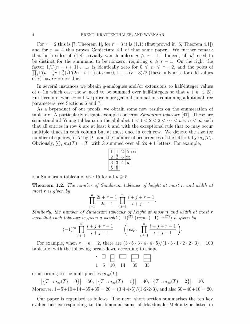
For r = 2 this is [7, Theorem 1], for r = 3 it is (1.1) (first proved in [6, Theorem 4.1])and for r = 4 this proves Conjecture 4.1 of that same paper. We further remarkthat both sides of (1.8) trivially vanish unless n > r − 1. Indeed, all k2

i need tobe distinct for the summand to be nonzero, requiring n > r − 1. On the right thefactor 1/Γ(n − i + 1)|i=r−1 is identically zero for 0 6 n 6 r − 2, and the poles of∏

i Γ(n− 12r+ 3

2)/Γ(2n− i+ 1) at n = 0, 1, . . . , (r−3)/2 (these only arise for odd values

of r) have zero residue.

In several instances we obtain q-analogues and/or extensions to half-integer valuesof n (in which case the ki need to be summed over half-integers so that n + ki ∈ Z).Furthermore, when γ = 1 we prove more general summations containing additional freeparameters, see Sections 6 and 7.

As a byproduct of our proofs, we obtain some new results on the enumeration oftableaux. A particularly elegant example concerns Sundaram tableaux [47]. These aresemi-standard Young tableaux on the alphabet 1 < 1 < 2 < 2 < · · · < n < n <∞ suchthat all entries in row k are at least k and with the exceptional rule that ∞ may occurmultiple times in each column but at most once in each row. We denote the size (ornumber of squares) of T by |T | and the number of occurrences of the letter k by mk(T ).Obviously,

∑kmk(T ) = |T | with k summed over all 2n+ 1 letters. For example,

1 1 2 5 ∞2 2 3 ∞3 3 4 ∞5 5

is a Sundaram tableau of size 15 for all n > 5.

Theorem 1.2. The number of Sundaram tableaux of height at most n and width atmost r is given by

n∏i=1

2i+ r − 1

2i− 1

n∏i,j=1

i+ j + r − 1

i+ j − 1.

Similarly, the number of Sundaram tableaux of height at most n and width at most rsuch that each tableaux is given a weight (−1)|T | (resp. (−1)m∞(T )) is given by

(−1)rnn∏

i,j=1

i+ j + r − 1

i+ j − 1

(resp.

n∏i,j=1

i+ j + r − 1

i+ j − 1

).

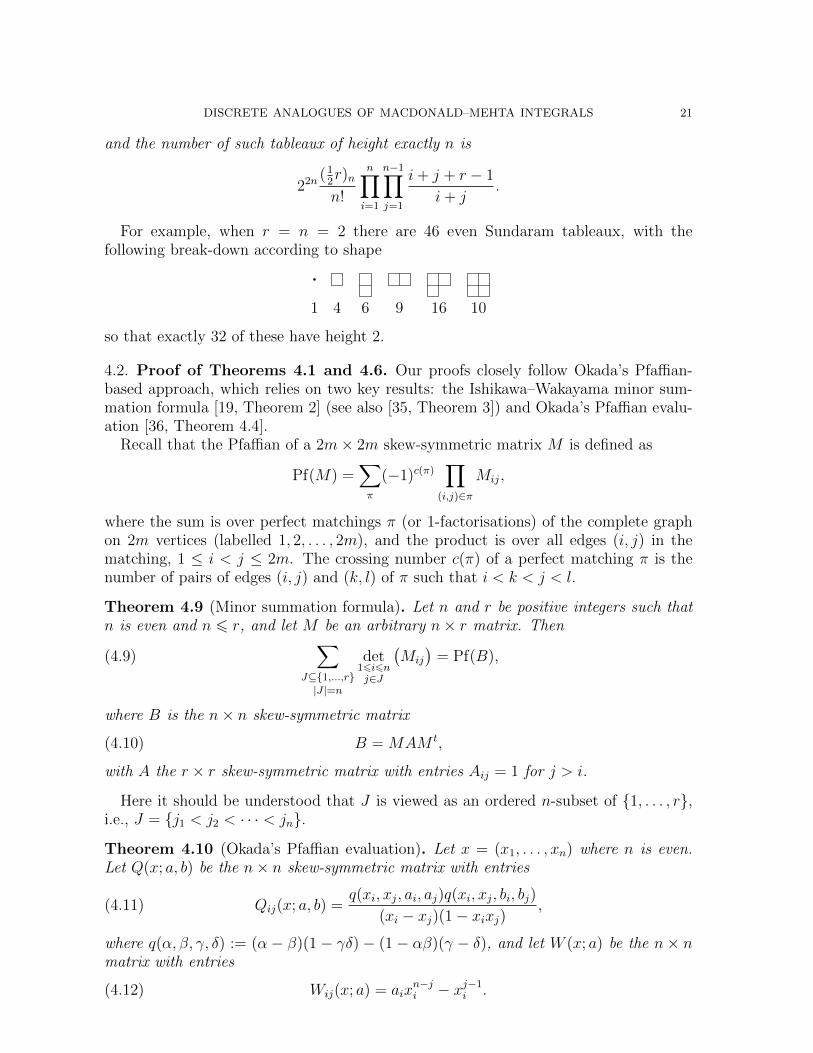
For example, when r = n = 2, there are (3 · 5 · 3 · 4 · 4 · 5)/(1 · 3 · 1 · 2 · 2 · 3) = 100tableaux, with the following break-down according to shape

1 5 10 14 35 35

or according to the multiplicities m∞(T ):∣∣{T : m∞(T ) = 0}∣∣ = 50,

∣∣{T : m∞(T ) = 1}∣∣ = 40,

∣∣{T : m∞(T ) = 2}∣∣ = 10.

Moreover, 1−5+10+14−35+35 = 20 = (3·4·4·5)/(1·2·2·3), and also 50−40+10 = 20.

Our paper is organised as follows. The next, short section summarises the ten keyevaluations corresponding to the binomial sums of Macdonald–Mehta-type listed in


Table 1. Section 3 reviews some standard material concerning classical group charactersneeded in our subsequent computations. Section 4 deals with summation identities fororthogonal and symplectic characters. Although several such identities were derivedpreviously by Okada [36], his results are not sufficient for our purposes, and morerefined identities as well as identities in which the summands have alternating signsare added to Okada’s list. In Section 5 we then apply the results from Section 4 toevaluate the sums Sr,n(α, 1

2, δ) claimed in Section 2. In most cases, we are able to also

provide q-analogues. Our evaluations of Sr,n(α, 1, δ) given in Section 2 are dealt with inSections 6 and 7. All these evaluations result from a single identity, a transformationformula between multiple elliptic hypergeometric series originally conjectured by thethird author [48, Conj. 6.1], and proven independently by Rains [43, Theorem 4.9] andby Coskun and Gustafson [9]. We do not present this formula in its full generalityhere, but restrict ourselves to stating the relevant (q-)special case in Theorem 6.1 atthe beginning of Section 6. The remainder of that section is devoted to proving ourevaluations of the sums Sr,n(2, 1, δ), while Section 7 is devoted to proving the evaluationsof the sums Sr,n(1, 1, δ). In all cases but one, we provide q-analogues which actuallycontain an additional parameter. The only exception is the sum Sr,n(1, 1, 1), wherewe are “only” able to establish a summation containing an additional parameter (seeProposition 7.2), but for which we were not able to find a q-analogue. Moreover, in thiscase we needed to take recourse to an ad hoc approach, since we could not figure outa way to use the aforementioned transformation formula. The final section, Section 8,discusses some further aspects of the work presented in this article, open problems, and(possible) further avenues.

To conclude the introduction, we point out two further articles addressing the multi-sums in [6]. First, in [28] the double sums considered in [6] are embedded into athree-parameter family of double sums, and it is shown that all of them can be explic-itly computed by using complex contour integrals or by the use of the computer algebrapackage Sigma [44], thus proving in particular all the respective conjectures in [6], in-cluding (1.2). Second, Bostan, Lairez and Salvy [3] recently presented an algorithmicapproach to finding recurrences for multiple binomial sums of the type considered inthis paper. Interestingly, complex contour integrals are again instrumental in this ap-proach. Among other things, it allowed them to prove automatically all the double-sumidentities from [6], again including all the conjectures from [6], such as (1.2). Moreover,their algorithmic approach is — in principle — capable of proving any of our r-fold sumidentities for fixed r. (As usual, “in principle” refers to the fact that today’s computersmay not actually be able to finish the required computations.) To come up with anautomatic proof for any of our identities for generic r seems however to be currentlyout of reach.

Acknowledgements. We thank Peter Forrester, Ron King, Soichi Okada and HelmutProdinger for helpful discussions. The second author also gratefully acknowledges theGalileo Galilei Institute of Theoretical Physics in Firenze, Italy, and to the National In-stitute of Mathematical Sciences, Daejeon, South Korea for the inspiring environmentsduring his visits in June/July 2015, when most of this work was carried out.


2. Summary of the ten primary identities

Here we summarise as succinctly as possible the ten product formulas for the dis-crete Macdonald–Mehta integral Sr,n(α, γ, δ) (defined in (1.7)), corresponding to theparameter choices listed in Table 1. Proofs and further generalisations are given inSections 4–7.

For α = 2 there are a total of seven cases, given by

(2.1) Sr,n(2, γ, δ)

=r∏i=1

Γ(1 + iγ)

Γ(1 + γ)·

Γ(2n+ 1) Γ(n− i− γ + χ+ 2) Γ((i− 1)γ + δ+12

)

Γ(n− i+ χ+ 1) Γ(n− iγ + χ+ 1) Γ(n− (i− 1)γ − δ−32− χ)

,

where χ = 1 if δ = 0, and χ = 0 otherwise. For α = 1 and δ = 0 there are two cases,given by

(2.2) Sr,n(1, γ, 0) = 22rn−γr(r−1)

r∏i=1

Γ(1 + iγ)

Γ(1 + γ)· Γ(2n+ 1) Γ(2n− i+ γ + 2)

Γ(2n− (i− 2)γ + 1) Γ(2n− i+ 2).

(This formula remains valid if γ = 0 or n is a half-integer.)The remaining case is

(2.3) Sr,n(1, 1, 1) = r!

dr/2e∏i=1

Γ2(i) Γ(2n+ 1)

Γ(n− i+ 1) Γ(n− i+ 2)

br/2c∏i=1

Γ(i) Γ(i+ 1) Γ(2n+ 1)

Γ2(n− i+ 1).

3. The Weyl character formula and Schur functions of type G

The purpose of this section is to collect standard material on classical group charactersthat we use in Sections 4 and 5.

3.1. Some simple q-functions. Assume that 0 < q < 1 and m,n are integers suchthat 0 6 m 6 n. Then the q-shifted factorial, q-binomial coefficient, q-gamma functionand q-factorial are given by

(a; q)n =n∏k=1

(1− aqk−1), (a; q)∞ =∞∏k=1

(1− aqk−1)[n

m

]=

[n

m

]q

=(qn−m+1; q)m

(q; q)m

Γq(x) = (1− q)1−x (q; q)∞(qx; q)∞

[n]q =1− qn

1− q, [n]q! = Γq(n+ 1) = [n]q [n− 1]q · · · [1]q.

We also need some generalisations of the q-shifted factorials to partitions. We usestandard terminology for partitions, as for example found in [31, Chapter 1], Moreprecisely, let λ be a partition, that is, λ = (λ1, λ2, . . . ) is a weakly decreasing sequenceof non-negative integers with only finitely many non-zero λi. The positive λi are calledthe parts of λ and the number of parts is called the length of the partition, denotedby l(λ). As usual we identify a partition with its (Young) diagram, and the conjugatepartition λ′ is the partition obtained by reflecting the diagram in the main diagonal. We


shall frequently need partitions of rectangular shape. By definition, this is a partitionall of whose parts are the same. In order to have a convenient notation, we write (rn)for the partition (r, r, . . . , r) with n occurrences of r. If λ is a partition of length atmost n and largest part at most r, we use the suggestive notation λ ⊆ (rn). Clearlythis is equivalent to λ′ ⊆ (nr). We say that (i, j) is a square (in the diagram) of λ andwrite (i, j) ∈ λ if and only if 1 6 i 6 l(λ) and 1 6 j 6 λi. Following [42], we now define

C−λ (a; q) =∏

(i,j)∈λ

(1− aqλi+λ′j−i−j)(3.1a)

C+λ (a; q) =

∏(i,j)∈λ

(1− aqλi−λ′j+j−i+1)(3.1b)

C0λ(a; q) =

∏(i,j)∈λ

(1− aqj−i).(3.1c)

Expressed in terms of ordinary q-binomial coefficients we have

C−λ (a; q) =n∏i=1

(aqn−i; q)λi∏

16i<j6n

1− aqj−i−1

1− aqλi−λj+j−i−1(3.2a)

C+λ (a; q) =

n∏i=1

(aq2−2i; q)2λi

(aq2−i−n; q)λi

∏16i<j6n

1− aq2−i−j

1− aqλi+λj−i−j+2(3.2b)

C0λ(a; q) =

n∏i=1

(aq1−i; q)λi ,(3.2c)

where n is an arbitrary integer such that l(λ) 6 n. Since conjugation simply inter-changes rows and columns of a partition, it follows readily from (3.1) that

C−λ′(a; q) = C−λ (a; q)(3.3a)

C+λ′(a; q) = (−aq)|λ|q3n(λ)−3n(λ′)C+

λ

(a−1q−2; q

)(3.3b)

C0λ′(a; q) = (−a)|λ|qn(λ)−n(λ′)C0

λ

(a−1; q

),(3.3c)

where |λ| := λ1 + λ2 + · · · and n(λ) :=∑

i>1(i− 1)λi =∑

i>1

(λ′i2

).

3.2. The Weyl character and dimension formulas. Let g be a complex semisimpleLie algebra of rank r, h and h∗ the Cartan subalgebra and its dual, and Φ the root systemspanning h∗ with basis of simple roots {α1, . . . , αr}, see e.g., [4,17]. Let 〈·, ·〉 denote theusual symmetric bilinear form on h∗, and assume the standard identification of h andh∗ through the Killing form so that the coroots are given by

α∨ =2α

〈α, α〉=

2α

‖α‖2.

Let ω1, . . . , ωr be the fundamental weights, i.e., 〈ωi, α∨j 〉 = δij, and denote the rootlattice Zα1 ⊕ · · · ⊕ Zαr and weight lattice Zω1 ⊕ · · · ⊕ Zωr by Q and P , respectively.Further, let P+ be the set of dominant (integral) weights,

P+ ={λ ∈ P : 〈λ, α∨i 〉 > 0 for 1 6 i 6 r

},


and set

Q+ ={α ∈ Q : 〈α∨, ωi〉 > 0 for 1 6 i 6 r

}.

We also denote the set of positive roots by Φ+, so that Φ+ = Q+ ∩ Φ.The irreducible highest weight modules V (λ) of g are indexed by dominant weights λ.

The characters corresponding to these modules are defined as

chV (λ) :=∑µ∈h∗

dim(Vµ) eµ,

where the Vµ are the weight spaces in the weight-space decomposition of V (λ) and eλ

for λ ∈ P is a formal exponential satisfying eλ eµ = eλ+µ. It is a well-known fact thatdim(Vλ) = 1 and dim(Vµ) = 0 if λ−µ 6∈ Q+. The characters can be computed explicitlyusing the Weyl character formula

(3.4) chV (λ) =

∑w∈W sgn(w) ew(λ+ρ)−ρ∏

α>0(1− e−α).

Here, W is the Weyl group of g, α > 0 is shorthand for α ∈ Φ+, and ρ = 12

∑α>0 α =∑r

i=1 ωi is the Weyl vector. For λ = 0, Weyl’s formula simplifies to the denominatoridentity

(3.5)∑w∈W

sgn(w) ew(ρ)−ρ =∏α>0

(1− e−α).

The dimension of the highest weight module V (λ) follows from the Weyl characterformula by applying the map eλ 7→ 1. We will require two slightly more general spe-cialisations resulting in q-dimension formulas. Let s be the squared length of the shortroots in Φ and define F and F∨ by

F : Z[e−α0 , . . . , e−αr ]→ Z[qs], F (e−αi) = q〈ρ,αi〉

F∨ : Z[e−α0 , . . . , e−αr ]→ Z[q], F∨(e−αi) = q〈ρ,α∨i 〉 = q

for all i with 1 6 i 6 r. By defining the q-dimensions by

dimq V (λ) := F(

e−λ chV (λ))

and dim∨q V (λ) := F∨(

e−λ chV (λ)),

we have the following pair of dimension formulas.

Lemma 3.1. We have

dimq V (λ) =∏α>0

1− q〈λ+ρ,α〉

1− q〈ρ,α〉,(3.6a)

dim∨q V (λ) =∏α>0

1− q〈λ+ρ,α∨〉

1− q〈ρ,α∨〉.(3.6b)

In the q → 1 limit, (3.6a) implies the Weyl dimension formula

dimV (λ) =∏α>0

〈λ+ ρ, α〉〈ρ, α〉

.


Proof. Applying F to e−λ chV (λ) ∈ Z[e−α1 , . . . , e−αr ] and using (3.4), we obtain

dimq V (λ) =

∑w∈W sgn(w)q−〈ρ,w(λ+ρ)−λ−ρ〉∏

α>0(1− q〈ρ,α〉).

Since 〈ρ, w(λ+ρ)〉 = 〈w−1(ρ), λ+ρ〉 and sgn(w) = sgn(w−1), a change of the summationindex from w to w−1 results in

dimq V (λ) =

∑w∈W sgn(w)q−〈w(ρ)−ρ,λ+ρ〉∏

α>0(1− q〈ρ,α〉).

The first claim now follows from the denominator formula (3.5) with e−u 7→ q−〈u,λ+ρ〉.The proof of (3.6b) is nearly identical and is left to the reader. �

In the next four subsections we restrict the Weyl character and dimension formulasto the four classical types and give “dual” forms for the q-dimension formulas neededin our proofs of the discrete Macdonald–Mehta integrals.

3.3. The Schur functions. For x = (x1, . . . , xn) and λ a partition of length at mostn, the Schur function sλ(x) is defined by

(3.7) sλ(x) :=det16i,j6n(x

λj+n−ji )

det16i,j6n(xn−ji ).

If Λn = Z[x1, . . . , xn]Sn denotes the ring of symmetric functions in n variables, thenthe Schur functions indexed by partitions of length at most n form a basis of Λn. TheSchur functions have a simple interpretation in terms of the representation theory ofthe symmetric group Sn and the general linear group GLn(C). More precisely, they areexactly the characters of the irreducible (polynomial) representations of GLn(C). Therepresentation theory of SLn(C) is almost identical to that of GLn(C), the only notabledifference being that in the former irreducible representations are indexed by partitionsof length at most n − 1, and to interpret such sλ(x) as a character we should imposethe restriction x1 · · ·xn = 1. Since the Schur function sλ(x) is homogeneous of degreeλ and satisfies

sλ(x) = (x1 · · ·xn)λns(λ1−λn,...,λn−1−λn,0)(x),

these differences do not affect any of the underlying combinatorics. In particular, if gis the Lie algebra sln(C) and φ the ring isomorphism

φ : Z[

eλ : λ ∈ P]W → Z

[x1, . . . , xn−1, x

−11 · · · x−1

n−1

]Sn= Λ′n(3.8a)

φ(eωi) = x1 · · ·xi for 1 6 i 6 n− 1,(3.8b)

then

(3.9) φ(

chV (λ))

= sλ(x)|xn=x−11 ···x

−1n−1,

where on the left λ is a dominant weight parametrised as

(3.10) λ = (λ1 − λ2)ω1 + · · ·+ (λn−2 − λn−1)ωn−2 + λn−1ωn−1

and on the right λ is the partition (λ1, . . . , λn−1, 0).


Instead of using the ratio of determinants given in (3.7), we can compute the Schurfunction in a more combinatorial fashion using semi-standard Young tableaux. Namely,

(3.11) sλ(x) =∑T

xT ,

where the sum is over all semi-standard Young tableaux T of shape λ on the alphabet

1 < 2 < · · · < n and xT := xm1(T )1 · · ·xmn(T )

n .From Lemma 3.1 and equation (3.9), it follows that for l(λ) 6 n we have the principal

specialisation formula

(3.12) sλ(1, q, . . . , qn−1) = qn(λ)

∏16i<j6n

1− qλi−λj+j−i

1− qj−i.

Indeed, since the above only depends on differences between the parts of λ, we mayassume without loss of generality that λn = 0. Since the set of positive roots is givenby

{αi + · · ·+ αj : 1 6 i 6 j 6 n− 1},it follows that for λ ∈ P+ parametrised by (3.10) we have

(3.13) dimq V (λ) = dim∨q V (λ) =∏

16i6j6n−1

1− qλi−λj+1+j−i+1

1− qj−i+1.

Since F (e−ωi) = qi(n−i)/2, it follows from (3.8b) that under the induced action of F onΛ′n we have

F (xi) = qi−(n+1)/2 for 1 6 i 6 n− 1.

We also have F (e−λ) = q(n−1)|λ|/2−n(λ), where on the right λ is the partition correspond-ing to λ ∈ P+ on the left. Hence,

sλ(1, q, . . . , qn−1) = q(n−1)|λ|/2sλ

(q−(n−1)/2, q−(n−3)/2, . . . , q(n−1)/2

)= q(n−1)|λ|/2F

(sλ(x)

)= qn(λ)F (e−λ chV (λ)) = qn(λ) dimq V (λ),

which by (3.13) implies (3.12). All of the above is well-known, although rarely madeexplicit. Since later we want to refer to analogous results for other groups withoutspelling out the (less well-known) details, we have included the full details of the Schurfunction case. We also note that each of the principal specialisation formulas for theclassical groups has a dual form obtained by using conjugate partitions. These dualforms will be crucial later.

Lemma 3.2 (Principal specialisation — dual form). For λ ⊆ (rn), we have

sλ(1, q, . . . , qn−1) = qn(λ)

r∏i=1

[n+ r − 1

λ′i + r − i

][n+ r − 1

r − i

]−1 ∏16i<j6r

1− qλ′i−λ′j+j−i

1− qj−i.

Proof. Perhaps the most elegant proof is to use the dual Jacobi–Trudi identity [31, p. 41]and the principal specialisation formula for the elementary symmetric functions [31,p. 27], combined with the the determinant evaluation [24, Theorem 26].


In view of the other types yet to be discussed, we will proceed in a slightly differentmanner. By (3.2), we can write (3.12) as

sλ(1, q, . . . , qn−1) = qn(λ)C

0λ(qn; q)

C−λ (q; q).

According to (3.3), the right-hand side also equals

(−qn)|λ|qn(λ′)C0λ′(q

−n; q)

C−λ′(q; q),

which, by (3.2) with n 7→ r, is

(−qn)|λ|qn(λ′)r∏i=1

(q1−i−n; q)λ′i(qr−i+1; q)λ′i

∏16i<j6r


1− qj−i.

By

(3.14)r∏i=1

(q1−i−n; q)λ′i(qr−i+1; q)λ′i

= (−qn)−|λ|qn(λ)−n(λ′)r∏i=1

(q; q)n+i−1(q; q)r−i(q; q)λ′i+r−i(q; q)n+i−λ′i−1

,

the lemma follows. �

3.4. The odd-orthogonal Schur functions. A sequence (λ1, . . . , λn) is called a half-partition if λ1 > λ2 > · · · > λn > 0 and λi ∈ Z + 1/2.

For x = (x1, . . . , xn) and λ = (λ1, . . . , λn) a partition or half-partition, the odd-orthogonal Schur functions are defined as (cf. [13, 29])

(3.15) so2n+1,λ(x) :=det16i,j6n

(xλj+n−j+1/2i − x−(λj+n−j+1/2)

i

)det16i,j6n

(xn−j+1/2i − x−(n−j+1/2)

i

) .

The so2n+1,λ(x) again arise from (3.4), this time for g = so2n+1(C). Defining φ by

φ : Z[

eλ : λ ∈ P]W → Z

[x±1/21 , . . . , x±1/2

n

]Bn

φ(e−ωi) =

{x1 · · ·xi, for 1 6 i 6 n− 1,

(x1 · · ·xn)1/2, for i = n,

where Bn is the hyperoctahedral group acting on the xi by permuting them and bysending xi to x−1

i for some i, we have

(3.16) φ(

chV (λ))

= so2n+1,λ(x),

where on the left λ is a dominant weight parametrised as

λ = (λ1 − λ2)ω1 + · · ·+ (λn−1 − λn)ωn−1 + 2λnωn,

and on the right λ is the partition or half-partition (λ1, . . . , λn).For later use, we will also define the companion

(3.17) so+2n+1,λ(x) :=

det16i,j6n

(xλj+n−j+1/2i + x

−(λj+n−j+1/2)i

)det16i,j6n

(xn−j+1/2i + x

−(n−j+1/2)i

) .

If λ is a partition, it readily follows that

(3.18) so+2n+1,λ(x) = (−1)|λ| so2n+1,λ(−x).


For half-partitions, however, so+2n+1,λ(x) is a rational function such that

so+2n+1,λ(x)D(x) ∈ Z[x±]Bn , D(x) :=

n∏i=1

(x1/2i + x

−1/2i ).

Since for half-partitions so2n+1,λ(x)D(x) ∈ Z[x±]Bn , it follows that, regardless of thetype of λ, we have

so2n+1,λ(x) so+2n+1,λ(x) ∈ Z[x±]Bn .

In terms of the Sundaram tableaux introduced on page 4, for λ a partition we have

so2n+1,λ(x) =∑T

xT ,

where the sum is over all Sundaram tableaux of shape λ and

(3.19) xT :=n∏k=1

xmk(T )−mk(T )k .

Lemma 3.3 (Principal specialisation — dual form). For λ ⊆ (rn) a partition, we have

(3.20a) so2n+1,λ(q, q2, . . . , qn) = qn(λ)−n|λ|

r∏i=1

[2n+ 2r − 1

λ′i + r − i

][2n+ 2r − 1

r − i

]−1

×∏

16i<j6r


1− qj−i· 1− q2n−λ′i−λ′j+i+j−1

1− q2n+i+j−1

and

(3.20b) so2n+1,λ(q1/2, q3/2, . . . , qn−1/2) = qn(λ)−(n−1/2)|λ|

×r∏i=1

1 + qn−λ′i+i−1/2

1 + qn+i−1/2

[2n+ 2r − 1

λ′i + r − i

][2n+ 2r − 1

r − i

]−1

×∏

16i<j6r


1− qj−i· 1− q2n−λ′i−λ′j+i+j−1

1− q2n+i+j−1.

Proof. Let ε1, . . . , εn be the standard unit vectors in Rn. Assuming the realisation{α1, . . . , αn} = {ε1 − ε2, . . . , εn−1 − εn, εn} for the simple roots of so2n+1(C) (see [17]),the fundamental weights and positive roots are given by

{ω1, . . . , ωn} = {ε1, ε1 + ε2, . . . , ε1 + · · ·+ εn−1,12(ε1 + · · ·+ εn)},

{α ∈ Φ : α > 0} = {εi : 1 6 i 6 n} ∪ {εi ± εj : 1 6 i < j 6 n}.


Hence, by (3.6b), (3.16) and F (xi) = qn−i+1, we have

so2n+1,λ(q, q2, . . . , qn) = qn(λ)−n|λ| dim∨q V (Λ)(3.21)

= qn(λ)−n|λ|n∏i=1

1− q2λi+2n−2i+1

1− q2n−2i+1

×∏

16i<j6n


1− qj−i· 1− qλi+λj+2n−i−j+1

1− q2n−i−j+1.

It follows from (3.2) that the right-hand side can be expressed in terms of the generalisedq-shifted factorials as

qn(λ)−n|λ| C0λ(qn,−qn, qn+1/2,−qn+1/2; q)

C−λ (q; q)C+λ (q2n−1; q)

,

where C0λ(a1, . . . , ak; q) = C0

λ(a1; q) · · ·C0λ(ak; q). By (3.3), this is also

(−qn+1)|λ|qn(λ′) C0λ′(q

−n,−q−n, q−n−1/2,−q−n−1/2; q)

C−λ′(q; q)C+λ′(q

−2n−1; q).

Again using (3.2), but now with n replaced by r, this is

(3.22) (−qn+r)|λ|qn(λ′)r∏i=1

(q1−i−2n−r; q)λ′i(qr−i+1; q)λ′i

∏16i<j6r


1− qj−i· 1− q2n−λi−λj+i+j−1

1− q2n+i+j−1.

By (3.14) with n 7→ 2n+ r, the first claim follows.The second specialisation (3.20b) follows in much the same way by applying (3.2)

and (3.3) to

so2n+1,λ(q1/2, q3/2, . . . , qn−1/2)(3.23)

= qn(λ)−(n−1/2)|λ| dimq V (Λ)

= qn(λ)−(n−1/2)|λ|n∏i=1

1− qλi+n−i+1/2

1− qn−i+1/2

×∏

16i<j6n



1− q2n−i−j+1. �

For later reference we also state the principal specialisation of so+2n+1,λ(x).

Lemma 3.4. For λ = (λ1, . . . , λn) a partition or half-partition, we have

(3.24) so+2n+1,λ(q

1/2, . . . , qn−1/2) = qn(λ)−(n−1/2)|λ|n∏i=1

1 + qλi+n−i+1/2

1 + qn−i+1/2

×∏

16i<j6n



1− q2n−i−j+1.


Proof. According to (3.5), the denominator identity for Bn (or so2n+1,λ(C)) is given by(see also [24, Equation (2.4)])

(3.25) det16i,j6n

(xn−j+1/2i − x−(n−j+1/2)

i

)= (−1)(

n+12 )

n∏i=1

x1/2−ni (1− xi)

∏16i<j6n

(xi − xj)(1− xixj).

Replacing xi by −xi (readers worried about a choice of branch-cut should first multiply

both sides by∏

i x−1/2i and later divide by this factor) and taking the transpose of the

determinant, we obtain (see also [24, Equation (2.6)])

(3.26) det16i,j6n

(xn−i+1/2j + x

−(n−i+1/2)j

)=

n∏i=1

x1/2−ni (1 + xi)

∏16i<j6n

(xi − xj)(1− xixj).

If we specialise xi = qn−i+1/2 (1 6 i 6 n) in (3.17), then we get(3.27)

so+2n+1,λ(q

1/2, . . . , qn−1/2) =det16i,j6n

(q(λj+n−j+1/2)(n−i+1/2) + q−(λj+n−j+1/2)(n−i+1/2)

)det16i,j6n

(q(n−j+1/2)(n−i+/2) + q−(n−j+1/2)(n−i+1/2)

) .

By (3.26) with xj = qλj+n−j+1/2 or xj = qn−j+1/2, both determinants on the right-handside can be expressed in product form, resulting in (3.24). �

3.5. The symplectic Schur functions. For x = (x1, . . . , xn) and λ a partition oflength at most n, the symplectic Schur functions are defined as

(3.28) sp2n,λ(x) :=det16i,j6n

(xλj+n−j+1i − x−(λj+n−j+1)

i

)det16i,j6n

(xn−j+1i − x−(n−j+1)

i

) .

If g = sp2n(C), then

φ(

chV (λ))

= sp2n,λ(x),

where φ(e−ωi) = x1 · · · xi (1 6 i 6 n) and

P+ 3 λ = (λ1 − λ2)ω1 + · · ·+ (λn−1 − λn)ωn−1 + λnωn.

To express this combinatorially, we need the symplectic tableaux of King and El-Sharkaway [20,21]. These are semi-standard Young tableaux on 1 < 1 < 2 < 2 < · · · <n < n such that all entries in row k are at least k. For example,

1 1 2 3 52 2 3 44 4 5

is a symplectic tableau for n > 5. The symplectic analogue of (3.11) then is

sp2n,λ(x) =∑T

xT ,

where the sum is over all symplectic tableaux of shape λ and xT is again given by (3.19).


Lemma 3.5 (Principal specialisation — dual form). For λ ∈ (rn), we have

(3.29a) sp2n,λ(q, q2, . . . , qn) = qn(λ)−n|λ|

r∏i=1

1− qn−λ′i+i

1− qn+i

[2n+ 2r

λ′i + r − i

][2n+ 2r

r − i

]−1

×∏

16i<j6r


1− qj−i· 1− q2n−λ′i−λ′j+i+j

1− q2n+i+j

and

(3.29b) sp2n,λ(q1/2, q3/2, . . . , qn−1/2)

= qn(λ)−(n−1/2)|λ|r∏i=1

1− q2(n−λ′i+i)

1− q2(n+i)

[2n+ 2r

λ′i + r − i

][2n+ 2r

r − i

]−1

×∏

16i<j6r


1− qj−i· 1− q2n−λ′i−λ′j+i+j

1− q2n+i+j.

Proof. If we take the simple roots to be {α1, . . . , αn} = {ε1 − ε2, . . . , εn−1 − εn, 2εn}(see [17]), then

{ω1, . . . , ωn} = {ε1, ε1 + ε2, . . . , ε1 + · · ·+ εn},{α ∈ Φ : α > 0} = {2εi : 1 6 i 6 n} ∪ {εi ± εj : 1 6 i < j 6 n}.

From Lemma 3.1, it then follows that

sp2n,λ(q, q2, . . . , qn) = qn(λ)−n|λ| dimq V (λ)(3.30a)

= qn(λ)−n|λ|n∏i=1

1− q2(λi+n−i+1)

1− q2(n−i+1)

×∏

16i<j6n



1− q2n−i−j+2

and

sp2n,λ(q1/2, q3/2, . . . , qn−1/2) = qn(λ)−(n−1/2)|λ| dim∨q V (Λ)

(3.30b)

= qn(λ)−(n−1/2)|λ|n∏i=1

1− qλi+n−i+1

1− qn−i+1

×∏

16i<j6n



1− q2n−i−j+2.

The rest of the proof is analogous to that of Lemma 3.3; we omit the details. �

3.6. The even-orthogonal Schur functions. Let a Dn partition be a weakly de-creasing sequence (λ1, . . . , λn) such that each λi ∈ Z or each λi ∈ Z + 1/2, and suchthat λn−1 > |λn|. If λ is a Dn partition then so is λ := (λ1, . . . , λn−1,−λn).


For x = (x1, . . . , xn) and λ a Dn partition, the even-orthogonal Schur functions aredefined by

(3.31) so2n,λ(x) :=∑

σ∈{±1}

det16i,j6n

(σx

λj+n−ji + x

−(λj+n−j)i

)det16i,j6n

(xn−ji + x

−(n−j)i

) .

We note that so2n,λ(x) = so2n,λ(x), where x := (x1, . . . , xn−1, x−1n ). Assuming g =

so2n(C), we have

φ(

chV (λ))

= so2n,λ(x),

where

φ(e−ωi) =

x1 · · ·xi, for 1 6 i 6 n− 2,

(x1 · · ·xn−1x−1n )1/2, for i = n− 1,

(x1 · · ·xn)1/2, for i = n,

and

P+ 3 λ = (λ1 − λ2)ω1 + · · ·+ (λn−1 − λn)ωn−1 + (λn−1 + λn)ωn.

For our purposes it is not enough to consider so2n,λ(x); we also need the closelyrelated even-orthogonal characters (cf. [22])

(3.32) o2n,λ(x) = uλdet16i,j6n

(xλj+n−ji + x

−(λj+n−j)i

)det16i,j6n

(xn−ji + x

−(n−j)i

) ,

where λ is a partition or half-partition and uλ = 1 if l(λ) < n and uλ = 2 if l(λ) = n.Note that

(3.33) o2n,λ(x) =

{so2n,λ(x), if l(λ) < n,

so2n,λ(x) + so2n,λ(x), if l(λ) = n.

Also the even-orthogonal characters can be expressed in terms of a tableau sum, see,e.g., [12, 41]. We will however not define these tableaux here and instead restrict ourattention to the simpler “even Sundaram tableaux” of [12]. An even Sundaram tableauis a semi-standard Young tableau on the alphabet 1 < 1 < 2 < 2 < · · · < n < n < ∞such that all entries in row k are at least k, with the exception that ∞ may occurmultiple times in each column but at most once in each row. Note that the onlydifference with the earlier definition of Sundaram tableaux is that entries in row k haveto be at least k instead of k. This implies that 1 cannot actually occur in an evenSundaram tableaux. Due to the absence of the letter 1, it is not known how to assignmonomials to even Sundaram tableaux so that they generate o2n,λ(x). It is howevershown in [12] that o2n,λ(1

n) correctly counts the number of even Sundaram tableaux ofshape λ.


Lemma 3.6. For λ a partition contained in (rn), we have

(3.34) o2n,λ(q1/2, q3/2, . . . , qn−1/2)

= qn(λ)−(n−1/2)|λ|r∏i=1

[2n+ 2r − 2

λ′i + r − i

][2n+ 2r − 2

r − i

]−1

×∏

16i<j6r


1− qj−i· 1− q2n−λ′i−λ′j+i+j−2

1− q2n+i+j−2.

There is a similar result for o2n,λ(1, q, . . . , qn−1), but this is not needed.

Proof. If we specialise xi = qn−i+1/2 in (3.32), with 1 6 i 6 n, and then use thedeterminant evaluation (3.26) with xj = qλj+n−j or xj = qn−j, we obtain

(3.35) o2n,λ(q1/2, q3/2, . . . , qn−1/2) = uλ q

n(λ)−(n−1/2)|λ|n∏i=1

1 + qλi+n−i

1 + qn−i

×∏

16i<j6n


1− qj−i· 1− qλi+λj+2n−i−j

1− q2n−i−j .

The rest of the proof follows that of Lemma 3.3. �

For later reference we note that it follows in much the same way from (3.25) and(3.26) that

(3.36) so2n,λ(q1/2, q3/2, . . . , qn−1/2)

= qn(λ)−(n−1/2)|λ|( n∏

i=1

1 + qλi+n−i

1 + qn−i+

n∏i=1

1− qλi+n−i

1 + qn−i

)×

∏16i<j6n


1− qj−i· 1− qλi+λj+2n−i−j

1− q2n−i−j .

4. Okada-type formulas

With the exception of type Ar−1, our proofs of the discrete analogues of Macdonald–Mehta integrals for γ = 1/2 given in the next section rely on formulas for the multi-plication of Schur functions of type g indexed by partitions of rectangular shape. Suchformulas have been given by Okada in [36]. We use several of his formulas, but we alsorequire additional ones. In the subsection below, we list all these results, and we presentthe (principal) specialisations of these formulas that we actually need. Subsection 4.2provides the proofs of the new results not contained in [36]. These proofs heavily relyon “preparatory results” from [36].

4.1. Main results. Our first result applies to g = so2n+1(C). Let so−2n+1,λ(x) :=so2n+1,λ(x).

Theorem 4.1. Let r be a non-negative integer, ε ∈ {−1, 1} and s := 12r. Then

(4.1)∑λ⊆(rn)

ε|λ| so2n+1,λ(εx) = so2n+1,(sn)(x) soσ2n+1,(sn)(x),


where the sum on the left is over partitions, and σ = − if ε = 1 and σ = + if ε = −1.

For ε = 1 this is (a special case of) Okada’s [36, Theorem 2.5(1)].Later we require (4.1) in principally specialised form as follows from (3.21), (3.23)

and (3.24) for λ = (sn).

Corollary 4.2. For r a non-negative integer and ε ∈ {−1, 1}, we have

(4.2a)∑λ⊆(rn)

so2n+1,λ(q, q2, . . . , qn) = q−r(

n+12 ) (qr+1; q2)n

(q; q2)n

n∏i,j=1

1− qi+j+r−1

1− qi+j−1

and

(4.2b)∑λ⊆(rn)

ε|λ| so2n+1,λ(εq1/2, εq3/2, . . . , εqn−1/2)

= q−rn2/2 (q(r+1)/2; q)n(εq(r+1)/2; q)n

(q1/2; q)n(εq1/2; q)n

n∏i,j=1i 6=j

1− qi+j+r−1

1− qi+j−1,

where λ is summed over partitions.

Letting q tend to 1 in (4.2a) (or the ε = 1 case of (4.2b)) yields the unweightedenumeration of Sundaram tableaux given in Theorem 1.2. Taking ε = −1 in (4.2b),then using

(q(r+1)/2; q)n(−q(r+1)/2; q)n(q1/2; q)n(−q1/2; q)n

=(qr+1; q2)n

(q; q2)n,

and finally letting q1/2 tend to ±1 gives∑T⊆(rn)

(−1)|T |(∓1)∑n

k=1(mk(T )+mk(T )) = (±1)rnn∏

i,j=1

i+ j + r − 1

i+ j − 1.

Since

|T | = m∞(T ) +n∑k=1

(mk(T ) +mk(T )

),

this results in the two weighted enumerations of that theorem.

Next we consider g = sp2n(C).

Theorem 4.3. Let r be a non-negative integer and s := b12rc, t := d1

2re. Then

(4.3)∑λ⊆(rn)

sp2n,λ(x) = sp2n,(sn)(x) so2n+1,(tn)(x).

This identity follows from [36, Theorem 2.5(1)] by observing that (see e.g. [41, Propo-sition A2.1(c)])

so2n+1,λ+1/2(x) = sp2n,λ(x)n∏i=1

(x1/2i + x

−1/2i ),

where λ+ 1/2 stands for (λ1 + 1/2, . . . , λn + 1/2). It is interesting to note that Proctor[39, Lemma 4, equation for A2n(mωr), case r = n] obtained this same sum from aspecialised Schur function. (In representation-theoretic terms: the restriction of an


SL2n+1(C)-character indexed by a rectangular shape to Sp2n(C) decomposes into thesum of symplectic characters indexed by all shapes contained in that rectangle; seealso [23, Equation (3.4)].) He used his result to prove the (at the time conjectured)formula for the number of symmetric self-complementary plane partitions contained ina given box.

Once again, use of (3.21) as well as (3.30) yields our second corollary.

Corollary 4.4. For r a non-negative integer, we have

(4.4a)∑λ⊆(rn)

sp2n,λ(q, q2, . . . , qn) = q−r(

n+12 )

n+1∏i=1

n∏j=1

1− qi+j+r−1

1− qi+j−1

and

(4.4b)∑λ⊆(rn)

sp2n,λ(q1/2, q3/2, . . . , qn−1/2) = q−rn

2/2

2n∏i=1

1− q(i+r)/2

1− qi/2n∏i=1

n−1∏j=1

1− qi+j+r

1− qi+j.

Letting q1/2 tend to ±1 in (4.4b) implies two counting formulas for symplectictableaux.

Theorem 4.5. The number of symplectic tableaux of height at most n and width atmost r is given by

(4.5)n+1∏i=1

n∏j=1

i+ j + r − 1

i+ j − 1

and the number of such tableaux weighted by (−1)|T | is

(−1)rnn∏i=1

i+ br/2ci

n∏i=1

n−1∏j=1

i+ j + r

i+ j.

For example, when r = n = 2 there are (3 · 42 · 52 · 6)/(1 · 22 · 32 · 4) = 50 symplectictableaux, with the following break-down according to shape

1 4 5 10 16 14

so that the signed enumeration is 1− 4 + 5 + 10− 16 + 14 = 10 = (2 · 3 · 4 · 5)/(1 · 22 · 3).We remark that (4.5) is not actually new, and it is implicit in [39] that the number

of symplectic tableaux contained in (rm) (0 6 m 6 n) is given by

2n−m+1∏i=1

m∏j=1

i+ j + r − 1

i+ j − 1.

See also [26, Theorem 7] for an equivalent statement in terms of vicious walkers (non-intersecting lattice paths).

Our final Okada-type formula involves the even-orthogonal as well as orthogonalcharacters.


Theorem 4.6. Let r be a positive integer. Then

(4.6a)∑λ⊆(rn)

so2n,λ(x) = so2n,(sn)(x) so2n+1,(sn)(x),

where s := 12r, and

(4.6b)∑λ⊆(rn)

l(λ)=n

o2n,λ(x) = o2n,(sn)(x) so2n+1,(tn)(x),

where s := 12(r + 1) and t := 1

2(r − 1).

We remark that (4.6b) also holds when the orthogonal characters are replaced byeven-orthogonal Schur functions, but in some sense this is a weakening of the result.In the other direction, the analogous result does not hold for (4.6a) in that we cannotreplace the even-orthogonal Schur functions by orthogonal characters.

By (3.23), (3.35) and (3.36), the above two identities result in the final corollary ofthis section.

Corollary 4.7. For r a positive integer, we have∑λ⊆(rn)

so2n,λ(q1/2, q3/2, . . . , qn−1/2)(4.7a)

= q−rn2/2 (qr/2+1/2; q)n

(q1/2; q)n

((−qr/2; q)n(−1; q)n

+(qr/2; q)n(−1; q)n

) n∏i=1

n−1∏j=1

1− qi+j+r−1

1− qi+j−1

and ∑λ⊆(rn)

l(λ)=n

o2n,λ(q1/2, q3/2, . . . , qn−1/2)(4.7b)

= 2q−rn2/2 (qr/2; q)n

(q1/2; q)n· (−qr/2+1/2; q)n

(−1; q)n

n∏i=1

n−1∏j=1

1− qi+j+r−1

1− qi+j−1.

If we let q → 1 in (4.7b), we obtain a closed-form expression for the number ofeven Sundaram tableaux of height exactly n and width at most r. From (3.33) andso2n,λ(x) = so2n,λ(x), it follows that

(4.8) o2n,λ(1n) = uλ so2n,λ(1

n).

Hence we can combine (4.7a) and (4.7b) to also obtain the enumeration of such tableauxcontained in (rn).

Theorem 4.8. The number of even Sundaram tableaux of height at most n and widthat most r is given by

22n−1 (12r + 1

2)n + (1

2r)n

n!

n∏i=1

n−1∏j=1

i+ j + r − 1

i+ j,


and the number of such tableaux of height exactly n is

22n (12r)n

n!

n∏i=1

n−1∏j=1

i+ j + r − 1

i+ j.

For example, when r = n = 2 there are 46 even Sundaram tableaux, with thefollowing break-down according to shape

1 4 6 9 16 10

so that exactly 32 of these have height 2.

4.2. Proof of Theorems 4.1 and 4.6. Our proofs closely follow Okada’s Pfaffian-based approach, which relies on two key results: the Ishikawa–Wakayama minor sum-mation formula [19, Theorem 2] (see also [35, Theorem 3]) and Okada’s Pfaffian evalu-ation [36, Theorem 4.4].

Recall that the Pfaffian of a 2m× 2m skew-symmetric matrix M is defined as

Pf(M) =∑π

(−1)c(π)∏

(i,j)∈π

Mij,

where the sum is over perfect matchings π (or 1-factorisations) of the complete graphon 2m vertices (labelled 1, 2, . . . , 2m), and the product is over all edges (i, j) in thematching, 1 ≤ i < j ≤ 2m. The crossing number c(π) of a perfect matching π is thenumber of pairs of edges (i, j) and (k, l) of π such that i < k < j < l.

Theorem 4.9 (Minor summation formula). Let n and r be positive integers such thatn is even and n 6 r, and let M be an arbitrary n× r matrix. Then

(4.9)∑

J⊆{1,...,r}|J |=n

det16i6nj∈J

(Mij

)= Pf(B),

where B is the n× n skew-symmetric matrix

(4.10) B = MAM t,

with A the r × r skew-symmetric matrix with entries Aij = 1 for j > i.

Here it should be understood that J is viewed as an ordered n-subset of {1, . . . , r},i.e., J = {j1 < j2 < · · · < jn}.

Theorem 4.10 (Okada’s Pfaffian evaluation). Let x = (x1, . . . , xn) where n is even.Let Q(x; a, b) be the n× n skew-symmetric matrix with entries

(4.11) Qij(x; a, b) =q(xi, xj, ai, aj)q(xi, xj, bi, bj)

(xi − xj)(1− xixj),

where q(α, β, γ, δ) := (α − β)(1 − γδ) − (1 − αβ)(γ − δ), and let W (x; a) be the n × nmatrix with entries

(4.12) Wij(x; a) = aixn−ji − xj−1

i .


Then

(4.13) Pf(Q(x; a, b)

)=

det(W (x; a)

)det(W (x; b)

)∏16i<j6n(xi − xj)(1− xixj)

.

Combining these two theorems we readily obtain the following result.

Corollary 4.11. Let n, r be positive integers such that n is even, ε ∈ {±1}, andM = M(a, ε) is the n× r matrix with entries

Mij = xj−ai − εx−j+ai .

Then∑J⊆{1,...,r}|J |=n

det16i6nj∈J

(Mij

)= (−1)n/2 det

16i,j6n

(xr/2+n/2−j−a+1i − εx−(r/2+n/2−a−j+1)

i

)

×det16i,j6n

(xr/2+n/2−j+1/2i − x−(r/2+n/2−j+1/2)

i

)det16i,j6n

(xn−j+1/2i − x−(n−j+1/2)

i

) .

Proof. A routine calculation using the summation of geometric series shows that for theabove choice of M , the matrix B in (4.10) is given by

Bij =∑

16k<l6r

(MikMjl −MilMjk

)=

(xixj)a−r

(1− xi)(1− xj)Qij

(x;xr, εxr−2a+1

),

where xa is shorthand for (xa1, . . . , xan). Since Pf(uiujvij) =

(∏i ui)

Pf(vij), we obtain

Pf(B) =

( n∏i=1

xa−ri

1− xi

)Pf(Q(x;xr, εxr−2a+1

))=

det(W (x;xr)

)det(W (x; εxr−2a+1)

)∏ni=1 x

r−ai (1− xi)

∏16i<j6n(xi − xj)(1− xixj)

.

Use of (4.12), the Bn Vandermonde determinant (3.25), and the fact that n is even andε2 = 1 completes the proof. �

Proof of Theorem 4.1. From (see, e.g., [36, Lemma 5.3(2)])

(4.14) limxn→0

xrn soσ2n+1,λ(x1, . . . , xn) =

{soσ2n−1,µ(x1, . . . , xn−1), if r = λ1,

0, if r > λ1,

for µ := (λ2, . . . , λn−1), it follows that, if we multiply both sides of (4.1) by xrn and letxn tend to zero, we obtain (4.1) with n replaced by n − 1. Hence it suffices to provethe claim for even values of n.

Let Sr denote the left-hand side of (4.1). From (3.18), it follows that

Sr =∑λ⊆(rn)

soσ2n+1,λ(x).

By (3.15) and (3.17), this can also be written as

Sr =

∑λ⊆(rn) det16i,j6n

(xλj+n−j+1/2i − εx−(λj+n−j+1/2)

i

)det16i,j6n

(xn−j+1/2i − εx−(n−j+1/2)

i

) .


If we replace the sum over λ by a sum over k1, . . . , kn via the substitution

λj = kn−j+1 − ρj − 1/2, for 1 6 j 6 n,

and reverse the order of the columns in the determinant, this leads to

Sr = (−1)(n2)

∑16k1<k2<···<kn6r+n

det16i,j6n

(xkj−1/2i − εx−(kj−1/2)

i

)det16i,j6n

(xn−j+1/2i − εx−(n−j+1/2)

i

) .Now assume that n is even. We can then apply Corollary 4.11 with r 7→ r + n anda = 1/2 to find

Sr =det16i,j6n

(xr/2+n−j+1/2i − εx−(r/2+n−j+1/2)

i

)det16i,j6n

(xn−j+1/2i − εx−(n−j+1/2)

i

)×

det16i,j6n

(xr/2+n−j+1/2i − x−(r/2+n−j+1/2)

i

)det16i,j6n

(xn−j+1/2i − x−(n−j+1/2)

i

) .

Finally, recalling (3.15) and (3.17), we obtain

Sr = soσ2n+1,(sn)(x) so2n+1,(sn)(x),

with s = 12r. �

Proof of Theorem 4.6. Equation 4.14 once again holds when soσ2n+1,λ is replaced byso2n,λ or o2n,λ, so that we may again take n to be even.

Let Sr and S ′r denote the left-hand sides of (4.6a) and (4.6b), respectively. Using(3.31) and (3.32) and making the substitutions{

Sr : λj = kn−j+1 − n+ j − 1,

S ′r : λj = kn−j+1 − n+ j,for 1 6 j 6 n,

we get

Sr = (−1)(n2)∑

σ∈{±1}

∑16k1<k2<···<kn6r+n

det1≤i,j≤n(σx

kj−1i + x

−(kj−1)i

)det1≤i,j≤n

(xn−ji + x

−(n−j)i

)and

S ′r = 2(−1)(n2)

∑16k1<k2<···<kn6r+n−1

det1≤i,j≤n(xkji + x

−kji

)det1≤i,j≤n

(xn−ji + x

−(n−j)i

) .By Corollary 4.11 with r 7→ r + n, a = 1, ε = −σ and r 7→ r + n − 1, a = 0, ε = −1,respectively, this yields

Sr =

∑σ∈{±1} det16i,j6n

(σx

r/2+n−ji + x

−(r/2+n−j)i

)det1≤i,j≤n

(xn−ji + x

−(n−j)i

)×

det16i,j6n

(xr/2+n/2−j+1/2i − x−(r/2+n/2−j+1/2)

i

)det16i,j6n

(xn−j+1/2i − x−(n−j+1/2)

i

)


and

S ′r = 2det16i,j6n

(xr/2+n−j+1/2i + x

−(r/2+n−j+1/2)i

)det1≤i,j≤n

(xn−ji + x

−(n−j)i

)×

det16i,j6n

(xr/2+n−ji − x−(r/2+n−j)

i

)det16i,j6n

(xn−j+1/2i − x−(n−j+1/2)

i

) ,where we have used that n is even. From (3.15) and (3.31), we see that the expressionfor Sr is exactly

so2n,(sn)(x) so2n+1,(sn)(x), s := 12r,

and that for S ′r

o2n,(sn)(x) so2n+1,(tn)(x), s := 12(r + 1), t := 1

2(r − 1). �

5. Discrete Macdonald–Mehta integrals for γ = 1/2

We will slightly extend our earlier definition (1.7) by considering Sr,n(α, γ, δ) for na non-negative integer or half-integer. In the latter case, the sum over k1, . . . , kr isassumed to range over half-integers, so that in both cases the ki are summed over{−n,−n+ 1, . . . , n}.

5.1. The evaluation of Sr,n(1, 12, 0). Instead of computing this sum directly, we first

consider a q-analogue.

Proposition 5.1 (Ar−1 summation). Let 0 < q < 1, r a positive integer and n aninteger or half-integer such that n > (r − 1)/2. Then

(5.1)n∑

k1,...,kr=−n

∏16i<j6r

∣∣[ki − kj]q∣∣ r∏i=1

q(ki+n−r+i)2/2

[2n

n+ ki

]

=r!

[r]q1/2 !

r∏i=1

(−q1/2; q1/2)i(−qi/2+1; q)2n−r

×r∏i=1

Γq(1 + 12i)

Γq(32)·

Γq(2n+ 1) Γq(2n− i+ 52)

Γq(2n− i+ 2) Γq(2n− 12i+ 2)

.

Taking the q → 1 limit, we arrive at (cf. (2.2))

Sr,n(1, 12, 0) =

n∑k1,...,kr=−n

∏16i<j6r

|ki − kj|r∏i=1

(2n

n+ ki

)(5.2)

= 22rn−(r2)

r∏i=1

Γ(1 + 12i)

Γ(32)·

Γ(2n+ 1) Γ(2n− i+ 52)

Γ(2n− i+ 2) Γ(2n− 12i+ 2)

.

The evaluation of S1,1(n) in [6, Equation (5.6)] is the special case r = 2 of this identity.


Proof of Proposition 5.1. Denote the sum on the left of (5.1) by fn,r. Since

q∑r

i=1(ki+n−r+i)2/2∏

16i<j6r

∣∣1− qki−kj ∣∣= q(n−1/2)(r

2)−2(r3)+

∑ri=1(ki+n−r+1)2/2

∏16i<j6r

∣∣qki − qkj ∣∣,the summand of fn,r is a symmetric function which vanishes unless all ki are pairwisedistinct. Anti-symmetrisation thus yields

fn,r =r!

(1− q)(r2)

∑n>k1>···>kr>−n

∏16i<j6r

(1− qki−kj

) r∏i=1

q(ki+n−r+i)2/2

[2n

n+ ki

].

We write this as a sum over partitions λ ⊆ (r2n−r+1) via

ki = λ′i − n+ r − i, 1 6 i 6 r.

Then

fn,r =r!

(1− q)(r2)

∑λ⊆(r2n−r+1)

qn(λ)+|λ|/2∏

16i<j6r

(1− qλ′i−λ′j+j−i) r∏

i=1

[2n

λ′i + r − i

].

By Lemma 3.2 and the fact that sλ is homogeneous of degree |λ|, this can be writ-ten as a sum over principally specialised Schur functions. Performing in addition thereplacement n 7→ (n+ r − 1)/2, we arrive at

f(n+r−1)/2,r =r!

(1− q)(r2)

∏16i<j6r

(1− qj−i

) r∏i=1

[n+ r − 1

r − i

]×∑λ⊆(rn)

sλ(q1/2, q3/2, . . . , qn−1/2

),

for n a non-negative integer. (When n = 0, the sum on the right should be interpretedas 1.) The sum can be computed by [31, p. 85]2∑

λ⊆(rn)

sλ(q1/2, q3/2, . . . , qn−1/2

)=

n∏i=1

1− qi+(r−1)/2

1− qi−1/2

∏16i<j6n

1− qr+i+j−1

1− qi+j−1.

Some elementary simplifications of the q-products and the subsequent replacement n 7→2n− r + 1 result in

fn,r =r!

(1− q)(r2)

(q(r+1)/2; q)2n−r+1

(q1/2; q)2n−r+1

r∏i=1

(q; q)2n(q; q)i−1(qi; q2)2n−r+1

(q; q)22n−i+1

.

To transform this into the claimed product over q-gamma functions is somewhat deli-cate. First we use (a2; q2)n = (a; q)n(−a; q)n to write

(q(r+1)/2; q)2n−r+1

(q1/2; q)2n−r+1

r∏i=1

(qi; q2)2n−r+1

(q; q)2n−i+1

=r∏i=1

(−qi/2; q)2n−r+1(q(i+1)/2; q)2n−r+1

(q; q)2n−i+1

.

2This is equivalent to MacMahon’s formula [32] for the generating function of symmetric planepartitions that fit in a box of size n× n× r, proved by Andrews [1] and Macdonald [31].


The first term in the numerator is wanted, but we further need to transform the othertwo terms as follows:

r∏i=1

(q(i+1)/2; q)2n−r+1

(q; q)2n−i+1

=r∏i=1

(−q1/2; q1/2)i−1(q3/2; q)2n−i+1

(q; q)i−1(qi/2+1; q)2n−i+1

· 1− q1/2

1− qi/2.

Putting all this together, we get

fn,r =r!

(1− q)(r2) [r]q1/2 !

r∏i=1

(−q1/2; q1/2)i(−qi/2+1; q)2n−r ·(q; q)2n(q3/2; q)2n−i+1

(q; q)2n−i+1(qi/2+1; q)2n−i+1

.

By the definition of the q-gamma function, the result now follows. �

5.2. The evaluation of Sr,n(2, 12, 1). Again we first consider a q-analogue.

Proposition 5.2 (Br summation). Let 0 < q < 1, r a positive integer and n an integeror half-integer such that n > r − 1/2. Then

(5.3)n∑

k1,...,kr=−n

∏16i<j6r

∣∣[ki − kj]q [ki + kj]q∣∣ r∏i=1

∣∣[ki]q∣∣ q(ki−r+i2 )−(dne−n

2 )[

2n

n+ ki

]

= 2rr!r∏i=1

(−q; q1/2)2n−2iΓq(i)

Γq(32)·

Γq(2n+ 1) Γq(dne − i+ 32)

Γq(2n− i+ 2) Γq(dne − i+ 1).

Taking the q → 1 limit and using r!∏r

i=1 Γ(i) =∏r

i=1 Γ(i+ 1), we obtain (cf. (2.1))

Sr,n(2, 12, 1) :=

n∑k1,...,kr=−n

∏16i<j6r

∣∣k2i − k2

j

∣∣ r∏i=1

|ki|(

2n

n+ ki

)(5.4)

= 2(2n+1)r−r(r+1)

r∏i=1

Γ(1 + i)

Γ(32)·

Γ(2n+ 1) Γ(n− i+ 32)

Γ(2n− i+ 2) Γ(n− i+ 1).

Equation (5.12) in [6] is the special case r = 2 of this identity.

Proof. Once again, the sum will be denoted by fn,r. This time the summand is sym-metric under signed permutations of the ki. Exploiting this hyperoctahedral symmetry,we obtain

fn,r =2rr!

(1− q)r2

∑n>k1>···>kr>0

∏16i<j6r

(1− qki−kj)(1− qki+kj)

×r∏i=1

(1− qki) q(ki−r+i

2 )−(dne−n2 )[

2n

n+ ki

].

We now set

(5.5) ki = n− i− λ′r−i+1 + 1, 1 6 i 6 r,

where λ is a partition contained in (rdne−r). If we then replace n 7→ bnc+ r and use thedual Cn specialisation formula (3.29a) in the integer-n case or the dual Bn specialisation


formula (3.20b) with q1/2 7→ −q1/2 in the half-integer case, we get

fn+r,r =2rr! qr(

n+12 )

(1− q)r2

(q; q)n+r

(q; q)n

r∏i=1

(q; q)2n+2r

(q; q)2n+2r−2i+2

∑λ⊆(rn)

sp2n,λ(q, q2, . . . , qn)

and

fn+r−1/2,r =2rr! qrn

2/2

(1− q)r2

(q1/2; q)n+r

(q1/2; q)n

r∏i=1

(q; q)2n+2r−1

(q; q)2n+2r−2i+1

×∑λ⊆(rn)

(−1)|λ| so2n+1,λ

(−q1/2,−q3/2, . . . ,−qn−1/2

),

where n is a non-negative integer. (The two sums on the right are again to be interpretedas 1 when n = 0.) By Corollaries 4.2 and 4.4, we can carry out the summations, resultingin

fn+r,r =2rr!

(1− q)r2

r∏i=1

(q; q)2n+2r(q; q)2n+i(q; q)i−1

(q; q)2n+2r−2i+2(q; q)2n+r−i

and

fn+r−1/2,r =2rr!

(1− q)r2

(q1/2; q)n+r

(q1/2; q)n

r∏i=1

(q; q)2n+2r−1(q; q)2n+i−1(q; q)i−1

(q; q)2n+2r−2i+1(q; q)2n+r−i

,

respectively. The replacement n 7→ n − r or n 7→ n − r + 1/2 and some elementarymanipulations lead to

fn,r =2rr!

(1− q)r2

r∏i=1

(−q1/2; q1/2)2n−2i+1(q1/2; q)dne−i+1(q; q)2n(q; q)i−1

(q; q)2n−i+1(q; q)dne−i.

The proof is completed by writing this in terms of q-gamma functions. �

5.3. The evaluation of Sr,n(2, 12, 0). We first restate Proposition 1.1, now including

the half-integral case (cf. (2.1)).

Proposition 5.3 (Dr summation). Let r be a positive integer and n an integer orhalf-integer such that n > r − 1. Then

Sr,n(2, 12, 0) =

n∑k1,...,kr=−n

∏16i<j6r

∣∣k2i − k2

j

∣∣ r∏i=1

(2n

n+ ki

)(5.6)

= 22rn−r(r−1) Γ(1 + 12r)

Γ(32)·

Γ(bnc − 12r + 3

2)

Γ(bnc+ 1)

×r−1∏i=1

Γ(i+ 1)

Γ(32)·

Γ(2n+ 1) Γ(bnc − i+ 32)

Γ(2n− i+ 1) Γ(bnc − i+ 1).

As already pointed out in the introduction, the special cases r = 2, 3, 4 cover [7,Theorem 1], and Theorem 4.1 and Conjecture 4.1 in [6], respectively.


When n is a half-integer, the identity (5.6) admits a q-analogue:

(5.7)n∑

k1,...,kr=−n

∏16i<j6r

∣∣[ki − kj]q [ki + kj]q∣∣ r∏i=1

q(ki−r+i+1/2

2 )[

2n

n+ ki

]

= 2r [2]nqr!

[r]q!· 1

(−q; q)n−r

r∏i=1

(−q; q1/2)2n−2i

Γq2(1 + 12r)

Γq(32)

r−1∏i=1

Γq(i+ 1)

Γq(32)

×Γq2(n− 1

2r + 1)

Γq(n+ 12)

r−1∏i=1

Γq(2n+ 1) Γq(n− i+ 1)

Γq(2n− i+ 1) Γq(n− i+ 12).

Proof. As usual, we denote the sum on the left by fn,r. Due to the hyperoctahedralsymmetry of the summand, we have

fn,r = r! · 2r∑

n>k1>···>kr>0

(1− 12δkr,0)

∏16i<j6r

(k2i − k2

j )r∏i=1

(2n

n+ ki

).

Since n+kr must be an integer, the effective lower bound is 1/2 when n is a half-integer.In this case (1− 1

2δkr,0) = 1.

Again we make the variable change (5.5). Due to the different lower bound comparedto the Br summation in Proposition 5.2, this means that we will now be summing overpartitions λ contained in rbnc−r+1. We also note that in the integer-n case (1− 1

2δkr,0)

transforms into

(5.8) (1− 12δλ′1,n−r+1) = (1− 1

2δl(λ),n−r+1).

Next we replace n 7→ dne+ r − 1. Note that this turns (5.8) into

(1− 12δl(λ),n) = u−1

λ ,

with uλ as in (3.32). In the integer-n case, we can then use (3.34) for q = 1 combinedwith (4.8) to find

fn+r−1,r = 2rr!r∏i=1

(2n+ 2r − 2)!

(2n+ 2r − 2i)!

∑λ⊆(rn)

so2n,λ(1n).

In the half-integer case, we can use the q = 1 instance of (3.20a). This results in

(5.9) fn+r−1/2,r = 2rr!r∏i=1

(2n+ 2r − 1)!

(2n+ 2r − 2i+ 1)!

∑λ⊆(rn)

so2n+1,λ(1n).

As before, the sums on the right are 1 when n = 0. Evaluation of these sums for generaln by the q = 1 cases of (4.7a) and (4.2b) (with ε = 1), respectively, gives

fn+r−1,r = 22n+r−1 (12r + 1

2)n

n!

r∏i=1

(2n+ 2r − 2)!

(2n+ 2r − 2i)!

r−1∏i=1

(2n+ i− 1)! (i+ 1)!

(n+ r − i)! (n+ r − i− 1)!

and

(5.10) fn+r−1/2,r(q) = 2r(1

2r + 1

2)n

(12)n

r∏i=1

(2n+ 2r − 1)! (2n+ i− 1)! i!

(2n+ 2r − 2i+ 1)! (n+ r − i)!2.


Replacing n 7→ n−r+1 or n 7→ n−r+1/2 and then expressing fn,r in terms of gammafunctions, we arrive at the right-hand side of (5.6).

The proof of the q-case for half-integer n proceeds along exactly the same lines, with(5.9) replaced by

fn+r−1/2,r(q) =2rr!

(1− q)r2−r qr(n+1

2 )r∏i=1

(q; q)2n+2r−1

(q; q)2n+2r−2i+1

∑λ⊆rn

so2n+1,λ(q, q2, . . . , qn).

and (5.10) by

fn+r−1/2,r(q) =2rr!

(1− q)r2−r(qr+1; q2)n

(q; q2)n

r∏i=1

(q; q)2n+2r−1(q; q)2n+i−1(q; q)i−1

(q; q)2n+2r−2i+1(q; q)2n+r−i

. �

5.4. The evaluation of Sr,n(2, 12, 2). This is the (α, γ) = (2, 1/2) case in Table 1. It

has no interpretation in terms of finite reflection groups. It is also the only case thatapparently does not admit a simple closed-form product formula for half-integer n.

Proposition 5.4. Let 0 < q < 1, r a positive integer and n an integer such that n > r.Then

(5.11)n∑

k1,...,kr=−n

∏16i<j6r

∣∣[ki − kj]q [ki + kj]q∣∣ r∏i=1

[ki]2q q

(ki−r+i−1)2/2

[2n

n+ ki

]

= 2rr!

[r]!q· (−1; q1/2)r+1(−qr/2+1; q)n−r

(−1; q)n−r

r+1∏i=1

(−q1/2; q1/2)i−1(−q1/2; q1/2)2n−i−r

(−q1/2; q1/2)2n−2i+2

×r∏i=1

Γ2q(1 + 1

2i)

Γq(12)·

Γq(2n+ 1) Γq(n− i+ 32)

Γq(n− i+ 1) Γ2q(n− 1

2i+ 1)

.

In the q → 1 limit, this becomes (cf. (2.1))

Sr,n(2, 12, 2) =

n∑k1,...,kr=−n

∏16i<j6r

∣∣k2i − k2

j

∣∣ r∏i=1

k2i

(2n

n+ ki

)(5.12)

= 2rr∏i=1

Γ2(1 + 12i)

Γ(12)·

Γ(2n+ 1) Γ(n− i+ 32)

Γ(n− i+ 1) Γ2(n− 12i+ 1)

.(5.13)

Equation (5.13) in [6] is the special case r = 2 of this identity.

Proof. If we denote the sum on the left by fn,r and define kr+1 := 0, then the summandof fn,r can be rewritten as[

2n

n

]−1 ∏16i<j6r+1

∣∣[ki − kj]q [ki + kj]q∣∣ r+1∏i=1

q(ki−r+i−1)2/2

[2n

n+ ki

].

Hence, after anti-symmetrisation and the variable change

ki = n− i− λ′r−i+2 + 1, 1 6 i 6 r + 1


(so that λ′1 := n− r), we obtain

fn+r−1,r−1 =2r−1(r − 1)! qrn

2/2

(1− q)r2+r

[2n+ 2r − 2

n+ r − 1

]−1 r∏i=1

(q; q)2n+2r−2

(q; q)2n+2i−2

×∑λ⊆(rn)

l(λ)=n

o2n,λ(q1/2, q3/2, . . . , qn−1/2),

where we have also used (3.34). Next we apply (4.7b) so that

fn+r−1,r−1 = 2r(r − 1)!(−q1/2; q1/2)2n−1(−q(r+1)/2; q)n

(−1; q)n

× (qr/2; q)n(q; q)n

[2n+ 2r − 2

n+ r − 1

]−1 r−1∏i=1

(q; q)2n+2r−2(q; q)2n+i−1(q; q)i(q; q)2n+2r−2i−2(q; q)n+r−i(q; q)n+r−i−1

.

The rest follows as in earlier cases. �

6. Discrete Macdonald–Mehta integrals for γ = 1 and α = 2

In this section, we present our results concerning evaluations of Sr,n(α, γ, δ) for γ = 1and α = 2. In contrast to the previous section, where identities for classical groupcharacters played a key role, here our starting point is a transformation formula forelliptic hypergeometric series. Along the lines of Section 5, in each case we shall startwith a q-analogue, from which the evaluations of Sr,n(2, 1, δ) for δ = 0, 1, 2, 3 follow by astraightforward q → 1 limit. An additional feature is that the identities in this sectiontypically contain an additional parameter.

We start with the p = 0, x = q special case of a transformation formula origi-nally conjectured by the third author [48, Conjecture 6.1] and proven independently byRains [43, Theorem 4.9] and by Coskun and Gustafson [9].

Theorem 6.1. Let a, b, c, d, e, f be indeterminates, m a non-negative integer, and r ≥ 1.Then

(6.1)∑

06k1<k2<···<kr6m

q∑r

i=1(2i−1)ki∏

16i<j6r

(1− qki−kj)2 (1− aqki+kj)2

×r∏i=1

(1− aq2ki) (a, b, c, d, e, f, λaq2−r+m/ef, q−m; q)ki(1− a) (q, aq/b, aq/c, aq/d, aq/e, aq/f, efqr−1−m/λ, aq1+m; q)ki

=r∏i=1

(b, c, d, ef/a; q)i−1

(λb/a, λc/a, λd/a, ef/λ; q)i−1

×r∏i=1

(aq; q)m (aq/ef ; q)m−r+1 (λq/e, λq/f ; q)m−i+1

(λq; q)m (λq/ef ; q)m−r+1 (aq/e, aq/f ; q)m−i+1

×∑

06k1<k2<···<kr6m

q∑r

i=1(2i−1)ki∏

16i<j6r

(1− qki−kj)2 (1− λqki+kj)2

×r∏i=1

(1− λq2ki) (λ, λb/a, λc/a, λd/a, e, f, λaq2−r+m/ef, q−m; q)ki(1− λ) (q, aq/b, aq/c, aq/d, λq/e, λq/f, efqr−1−m/a, λq1+m; q)ki

,


where λ = a2q2−r/bcd.

In the above formula, we let m→∞ to obtain

(6.2)∑

06k1<k2<···<kr

q∑r

i=1(2i−1)ki∏

16i<j6r


×r∏i=1

( a2

q2r−3bcdef

)ki (1− aq2ki) (a, b, c, d, e, f ; q)ki(1− a) (q, aq/b, aq/c, aq/d, aq/e, aq/f ; q)ki

=r∏i=1

(b, c, d, ef/a; q)i−1

(λb/a, λc/a, λd/a, ef/λ; q)i−1

(aq, aq/ef, λq/e, λq/f ; q)∞(λq, λq/ef, aq/e, aq/f ; q)∞

×∑

06k1<k2<···<kr

q∑r

i=1(2i−1)ki∏

16i<j6r

(1− qki−kj)2 (1− λqki+kj)2

×r∏i=1

( a

qr−1ef

)ki (1− λq2ki) (λ, λb/a, λc/a, λd/a, e, f ; q)ki(1− λ) (q, aq/b, aq/c, aq/d, λq/e, λq/f ; q)ki

.

The two specialisations which are relevant for us are b = aq/c and b = aq2/c. Thecase b = aq/c (which has the effect of generating terms (λd/a; q)ki = (q1−r; q)ki in theright-hand side sum of (6.2), in turn implying that the only choice for the summationindices ki to produce a non-vanishing summand is ki = i− 1 for i = 1, 2, . . . , r) gives

(6.3)∑

06k1<k2<···<kr

q∑r

i=1(2i−1)ki∏

16i<j6r


×r∏i=1

( a

q2r−2def

)ki (1− aq2ki) (a, d, e, f ; q)ki(1− a) (q, aq/d, aq/e, aq/f ; q)ki

= q−(r3)( aef

)(r2)

r∏i=1

(q, d, e, f, ef/a, aqi−r/d; q)i−1 (aq2−r/d; q)2i−2

(aq/d, aq2−r/de, aq2−r/df, defqr−1/a; q)i−1

×r∏i=1

(aq, aq/ef, aq2−r/de, aq2−r/df ; q)∞(aq2−r/d, aq2−r/def, aq/e, aq/f ; q)∞

.

The case where b = aq2/c (which has the effect of generating terms (λd/a; q)ki =(q−r; q)ki in the right-hand side sum of (6.2), in turn implying that the only choices forthe summation indices ki to produce a non-vanishing summand are ki = i−1+χ(i > s)for some non-negative integer s, and i = 1, 2, . . . , r; here, χ(A) = 1 if A is true andχ(A) = 0 otherwise) gives

(6.4)∑

06k1<k2<···<kr

q∑r

i=1(2i−1)ki∏

16i<j6r


×r∏i=1

( a

q2r−1def

)ki (1− aq2ki) (1− cqki−1) (1− aqki+1/c) (a, d, e, f ; q)ki(1− a) (1− c/q) (1− aq/c) (q, aq/d, aq/e, aq/f ; q)ki

= (−1)rq2(r+13 )( a

qr−1ef

)(r+12 ) (aq2−r/cd)r (cq−r/d)r

(1− aq/c)r (1− c/q)r (q; q)r (aq1−r/d)2r


×r∏i=1

(q, e, f, aqi−r/d; q)i (d, ef/a; q)i−1 (aq1−r/d; q)2i

(aq/d, aq1−r/de, aq1−r/df ; q)i (defqr/a; q)i−1

×r∏i=1

(aq, aq/ef, aq1−r/de, aq1−r/df ; q)∞(aq1−r/d, aq1−r/def, aq/e, aq/f ; q)∞

×r∑s=0

(1− aq−r

dq2s)(

1− aq−r

d

) (aq−r/d, c/q, aq/c, aq1−r/de, aq1−r/df, q−r; q)s(q, aq2−r/cd, cq−r/d, e, f, aq/d; q)s

(qrefa

)s.

This is a transformation formula between a multiple basic hypergeometric series asso-ciated with the root system BCr and a very-well-poised basic hypergeometric 8φ7-series(see [15] for terminology).

6.1. The evaluation of Sr,n(2, 1, 0).

Proposition 6.2 (Dr summation). Let q be a real number with 0 < q < 1. For allnon-negative integers or half-integers m and n and a positive integer r, we have

(6.5)n∑

k1,...,kr=−n

∏16i<j6r

[kj − ki]2q [ki + kj]2q

r∏i=1

qk2i−(2i− 3

2)ki

1 + qki

1 + q

[2n

n+ ki

]q

[2m

m+ ki

]q

= r!( 2

[2]q

)rq−2(r+1

3 )+ 12(r

2)r∏i=1

Γq1/2(2i− 1) Γq(2n+ 1) Γq(2m+ 1)

Γq(m+ n− i+ 2) Γq(m+ n− i− r + 3)

·Γq1/2(2m+ 2n− 2i− 2r + 5)

Γq1/2(2n− 2i+ 3) Γq1/2(2m− 2i+ 3).

Taking the q → 1 limit, dividing both sides of the result by(

2mm

)r, and finally taking

the limit m→∞, we arrive at (cf. (2.1))

Sr,n(2, 1, 0) =n∑

k1,...,kr=−n

∏16i<j6r

(k2i − k2

j )2

r∏i=1

(2n

n+ ki

)(6.6)

= 22r(n−r+1)Γ(r + 1)r−1∏i=1

Γ(2i+ 1) Γ(2n+ 1)

Γ(2n− 2i+ 1).

The evaluation of W2(n) provided after the proof of Theorem 3.2 in [6] is the specialcase r = 2 of this identity.

Proof. To begin with, we observe that the summand of the sum on the left-hand sideof (6.5) is invariant under permutations of the summation indices. Indeed, writingS1(k1, k2, . . . , kr) for this summand, for a permutation σ of {1, 2, . . . , r} we have

(6.7) S1(kσ(1), kσ(2), . . . , kσ(r)) = qE1(σ;k1,k2,...,kr)S1(k1, k2, . . . , kr),

where

(6.8) E1(σ; k1, k2, . . . , kr) = 2∑

16i<j6r

χ(σ(i) > σ(j)

)(kσ(j)− kσ(i)

)− 2

r∑i=1

(ikσ(i)− iki).


Here, as before, χ(A) = 1 if A is true and χ(A) = 0 otherwise. Let Iσ(i) denote thenumber of indices j with 1 6 i < j 6 r and σ(i) > σ(j). Then, by elementary counting,we have

∑16i<j6r

χ(σ(i) > σ(j)

)(kσ(j) − kσ(i)) =

r∑j=1

(j − σ(j) + Iσ(j)

)kσ(j) −

r∑i=1

Iσ(i)kσ(i)

=r∑i=1

(i− σ(i))kσ(i).

If this is substituted back in (6.8), then one obtains E1(σ; k1, k2, . . . , kr) = 0. In combi-nation with (6.7), this implies the claimed invariance of summands under permutationsof the summation indices. As a consequence, we may restrict the range of summationon the left-hand side of (6.5) to k1 < k2 < · · · < kr, and in turn multiply this restrictedsum by r!, thereby not changing the value of the left-hand side of (6.5).

Now, in this (restricted) sum, we replace ki by ki − n, and we rewrite the arisingmultiple sum in terms of q-shifted factorials. The result is

r! qrn2+(r2− r

2)n(1 + q−n)r

(1− q)2r2−2r (1 + q)r

[2m

m− n

]rq

∑06k1<···<kr

∏16i<j6r

(1− qki−kj

)2 (1− qki+kj−2n

)2

·r∏i=1

(q−2n,−q1−n, q−m−n; q)ki(q,−q−n, qm−n+1; q)ki

q(2i−2r+m+n+ 12

)ki ,

where the summation indices ki now run over integers. Thus, we see that we may apply(6.3) with a = q−2n, d = q−m−n, e = q−n, f = q−n+1/2 to evaluate this sum. We have tobe a little careful though because of the appearance of the ratio (aq; q)∞/(aq/e; q)∞ onthe right-hand side of (6.3), which becomes the indeterminate expression 0/0 for theabove choices of a and e. To be precise, in (6.3) we have to first choose e =

√a, and

subsequently calculate the limit as a tends to q−2n. Doing this, we obtain

lima→q−2n

(aq; q)∞(√aq; q)∞

= lima→q−2n

(aq; q)2n−1 (1− aq2n) (aq2n+1; q)∞(√aq; q)n−1 (1−

√aqn) (

√aqn+1; q)∞

(6.9)

= 2(q1−2n; q)2n−1

(q1−n; q)n−1

= 2 (q1−2n; q)n.

After considerable simplification and rewriting of the right-hand side of (6.3) under theabove specialisation, we obtain the right-hand side of (6.5). �



Proposition 6.3. Let q be a real number with 0 < q < 1. For all non-negative integersm and n and a positive integer r, we have

(6.10)n∑

k1,...,kr=−n

∏16i<j6r


r∏i=1

qk2i−(2i−1)ki

∣∣[ki]q2

∣∣[ 2n

n+ ki

]q

[2m

m+ ki

]q

= r!( 2

[2]q

)rq−2(r+1

3 )r∏i=1

(Γ2q(i) Γq(2n+ 1)

Γq(n− i+ 2) Γq(n− i+ 1)

× Γq(2m+ 1)

Γq(m− i+ 2) Γq(m− i+ 1)· Γq(m+ n− i− r + 2)

Γq(m+ n− i+ 2)

).


2mm

)r, and finally per-

forming the limit m→∞, we obtain (cf. (2.1))

Sr,n(2, 1, 1) =n∑

k1,...,kr=−n

∏16i<j6r

(k2i − k2

j )2

r∏i=1

|ki|(

2n

n+ ki

)(6.11)

=r∏i=1

Γ(i) Γ(i+ 1) Γ(2n+ 1)

Γ(n− i+ 2) Γ(n− i+ 1).

Proof. Here, the summand of the multiple sum on the left-hand side of (6.10) is invariantunder both permutations of the summation indices and under replacement of ki by −ki,for some fixed i. To show this, if S2(k1, k2, . . . , kr) denotes the summand, then we have

S2(k1, . . . , ki−1,−ki, ki+1, . . . , kr) = qE2(k1,k2,...,kr)S2(k1, k2, . . . , kr),

where

E2(k1, k2, . . . , kr) = 2∑

16i<j6r

(−kj − ki) + 2∑

16i<j6r

(−kj + ki) +r∑i=1

(2(2i− 1)ki − 2ki

)= 4

r∑j=1

(−(j − 1)kj

)+

r∑i=1

(4i− 4)ki = 0.

This proves the invariance of S2(k1, k2, . . . , kr) under the replacement ki → −ki. As aconsequence, we may restrict the range of summation on the left-hand side of (6.10) to1 6 k1 < k2 < · · · < kr, and in turn multiply this restricted sum by 2rr!, thereby notchanging the value of the left-hand side of (6.10).

In this (restricted) sum, we replace ki by ki + 1, and we rewrite the arising multiplesum in terms of q-shifted factorials. The result is

2rr!

qr2−r(1− q)2r2−2r

[2n

n+ 1

]rq

[2m

m+ 1

]rq

∑06k1<···<kr

∏16i<j6r

(1− qki−kj

)2 (1− qki+kj+2

)2

·r∏i=1

(q2,−q2, q1−n, q1−m; q)ki(q,−q, qn+2, qm+2; q)ki

q(2i−2r+m+n)ki .


Thus, we see that we may apply (6.3) with a = q2, d = q1−n, e = q1−m, f = q to evaluatethis sum. After considerable simplification and rewriting, we obtain the right-hand sideof (6.10). �

Proposition 6.4. Let q be a real number with 0 < q < 1. For all positive half-integersm and n and a positive integer r, we have

(6.12)n∑

k1,...,kr=−n

∏16i<j6r


r∏i=1

qk2i−(2i−1)ki

∣∣[ki]q2

∣∣[ 2n

n+ ki

]q

[2m

m+ ki

]q

= r!( 2

[2]q

)rq−

14(2r+1

3 )r∏i=1

(Γ2q(i) Γq(2n+ 1)

Γ2q(n− i+ 3

2)

× Γq(2m+ 1)

Γ2q(m− i+ 3

2)· Γq(m+ n− i− r + 2)

Γq(m+ n− i+ 2)

).

Proof. This can be proved in the same way as Proposition 6.3. The only differences arethat, here, the summation index ki is replaced by ki + 1

2, i = 1, 2, . . . , r, and that the

relevant specialisation of (6.3) is a = q, d = q1/2−n, e = q1/2−m, f = q. �

From now on, all proofs are similar to one of the proofs of Propositions 6.2–6.4,except for the proof of Proposition 6.7. For the remaining theorems in this section(except for Proposition 6.7), we therefore content ourselves with specifying which choiceof parameters in (6.3) has to be used, without providing further details.


Proposition 6.5 (Br summation). Let q be a real number with 0 < q < 1. For allnon-negative integers or half-integers m and n and a positive integer r, we have

(6.13)n∑

k1,...,kr=−n

∏16i<j6r


r∏i=1

qk2i−(2i− 1

2)ki∣∣[ki]q2 [ki]q

∣∣[ 2n

n+ ki

]q

[2m

m+ ki

]q

= r!( 2

[2]q

)r[2]−r

q1/2 q−2(r+1

3 )− 12(r+1

2 )r∏i=1

(Γq1/2(2i) Γq(2n+ 1) Γq(2m+ 1)

Γq(m+ n− i+ 2) Γq(m+ n− i− r + 2)

×Γq1/2(2m+ 2n− 2i− 2r + 3)

Γq1/2(2n− 2i+ 2) Γq1/2(2m− 2i+ 2)

).


2mm



Sr,n(2, 1, 2) =n∑

k1,...,kr=−n

∏16i<j6r

(k2i − k2

j )2

r∏i=1

k2i

(2n

n+ ki

)(6.14)

= 2r(2n−2r−1)

r∏i=1

Γ(2i+ 1) Γ(2n+ 1)

Γ(2n− 2i+ 2).

Proof. The special case of (6.3) which is relevant here is a = q−2n, d = q−m−n, e = q−n+1,and f = q−n+1/2. �



Proposition 6.6. Let q be a real number with 0 < q < 1. For all non-negative integersm and n and a positive integer r, we have

(6.15)n∑

k1,...,kr=−n

∏16i<j6r


r∏i=1

qk2i−2iki

∣∣[ki]q2 [ki]2q

∣∣[ 2n

n+ ki

]q

[2m

m+ ki

]q

= r!( 2

[2]q

)rq−2(r+1

3 )−(r+12 )

r∏i=1

(Γq(2n+ 1)

Γ2q(n− i+ 1)

· Γq(2m+ 1)

Γ2q(m− i+ 1)

× Γq(i) Γq(i+ 1) Γq(m+ n− i− r + 1)

Γq(m+ n− i+ 2)

).


2mm



Sr,n(2, 1, 3) =n∑

k1,...,kr=−n

∏16i<j6r

(k2i − k2

j )2

r∏i=1

|ki|3(

2n

n+ ki

)(6.16)

=r∏i=1

Γ2(i+ 1) Γ(2n+ 1)

Γ2(n− i+ 1).

Proof. The special case of (6.3) which is relevant here is a = q2, d = q1−n, e = q1−m,and f = q2. �

Proposition 6.7. Let q be a real number with 0 < q < 1. For all positive half-integersm and n and a positive integer r, we have

n∑k1,...,kr=−n

∏16i<j6r


r∏i=1

qk2i−2iki

∣∣[ki]q2 [ki]2q

∣∣ [ 2n

n+ ki

]q

[2m

m+ ki

]q

(6.17)

= r!( 2

[2]q

)rq−2(r+1

3 )− r2

2− r

4

r∏i=1

(Γq(2n+ 1)

Γ2q(n− i+ 3

2)· Γq(2m+ 1)

Γ2q(m− i+ 3

2)

× Γq(i) Γq(i+ 1) Γq(m+ n− i− r + 1)

Γq(m+ n− i+ 2)

)×

r∑s=0

(√q; q)2

s

(1− q)2s

[n− s− 1/2]q! [m− s− 1/2]q!

[n− r − 1/2q! [m− r − 1/2]q!

[r

s

]q

[m+ n− r

s

]q

.

Proof. We start in the same way as in the proof of Proposition 6.3, observing thatthe summand on the left-hand side of (6.17) is invariant under permutations of thesummation indices ki and under replacement of ki by −ki, for some fixed i. This allowsone to concentrate on the range

1

26 k1 < k2 < · · · < kr.

The final result is then obtained by multiplying the sum over this range by 2rr!.


Next we replace ki by ki + 12

for i = 1, 2, . . . , r, and rewrite the resulting sum usingq-shifted factorials, to obtain

1

(1− q)2r2−2r

[2n

n+ 1/2

]rq

[2m

m+ 1/2

]rq

∑06k1<···<kr

∏16i<j6r

(1− qki−kj)2 (1− qki+kj+1)2

×r∏i=1

(q(2i−1)ki−i+1/4+ki(m+n−2r) (1− q2ki+1) (1− qki+1/2)2 (q, q1/2−n, q1/2−m; q)ki

(1− q2) (1− q)2 (q, q3/2+n, q3/2+m; q)ki

).

We may now transform the multiple sum on the right using (6.4) with a = q, c = q3/2,d = q, e = q1/2−n and f = q1/2−m. Using the standard basic hypergeometric notation

φr s

[a1, . . . , arb1, . . . , bs

; q, z

]=∞∑`=0

(a1, . . . , ar; q)`(q, b1, . . . , bs; q)`

((−1)`q(

`2))s−r+1

z`,

where (a1, . . . , ak; q)` = (a1; q)` · · · (ak; q)`, we obtain that this sum equals

F (m,n, r) φ8 7

[q−r, q1−r/2,−q1−r/2, q1/2−r+n, q1/2−r+m, q1/2, q1/2, q−r

q−r/2,−q−r/2, q1/2−n, q1/2−m, q1/2−r, q1/2−r, q; q, qr−m−n

],

where F (m,n, r) is an explicit product, suppressed here in order to focus on the essentialpart in the expression. To the above φ8 7-series, we may apply Watson’s transformationformula between a very-well-poised φ8 7-series and a balanced φ4 3-series (see [15, Ap-pendix (III.17)])

φ8 7

[a, q√a,−q

√a, b, c, d, e, f√

a,−√a, aq/b, aq/c, aq/d, aq/e, aq/f

; q,a2q2

bcdef

]=

(aq, aq/de, aq/df, aq/ef ; q)∞(aq/d, aq/e, aq/f, aq/def ; q)∞

φ4 3

[aq/bc, d, e, f

aq/b, aq/c, def/a; q, q

],

provided the φ8 7-series converges and the φ4 3-series terminates. It is then a routine buttedious task to convert the resulting expression into the right-hand side of (6.17). �

7. Discrete Macdonald–Mehta integrals for γ = 1 and α = 1

The purpose of this section is to present our evaluations of Sr,n(α, γ, δ) for γ =α = 1. In principle, it would seem that such evaluations could also follow from thetransformation formula in Theorem 6.1, by considering a limit case where a → 0.Indeed, the case δ = 0, that is, the evaluation of the sum Sr,n(1, 1, 0), is covered by(6.1), and it also produces a q-analogue containing a further parameter. Alas, all ourattempts to come up with appropriate further specialisations that would produce thesum Sr,n(1, 1, δ) with δ = 1 on the left-hand side of (6.1) failed. Hence, in orderto achieve the corresponding summation, we designed an ad hoc approach combiningthe evaluation of certain Vandermonde- and Cauchy-like determinants with summationformulas from the theory of hypergeometric series. As opposed to the case δ = 0, forδ = 1 we were not able to find a q-analogue.

It is interesting to note that the limit case a → 0 of (6.1) has been worked outearlier in [27, Equation (3.7)], where it was used for the enumeration of standard Youngtableaux of certain skew shapes. As is pointed out there, that limit case had explicitlyappeared even earlier in [25], where two different proofs had been given (one using a


specialisation of an identity for Schur functions, the other using a specialisation of aq-integral evaluation due to Evans), and where it had been applied in an again differentcontext, namely that of the enumeration of domino tilings.


Proposition 7.1 (Ar−1 summation). Let q be a real number with 0 < q < 1. For allnon-negative integers or half-integers m and n and a positive integer r, we have

(7.1)n∑

k1,...,kr=−n

∏16i<j6r

[kj − ki]2qr∏i=1

qk2i +(m+n−2i+2)ki

[2n

n+ ki

]q

[2m

m+ ki

]q

= r! q−rmn−16r(r−1)(2r−3m−3n−1)

×r∏i=1

Γq(i) Γq(2n+ 1) Γq(2m+ 1) Γq(2m+ 2n− r − i+ 3)

Γq(2n− i+ 2) Γq(2m− i+ 2) Γ2q(m+ n− i+ 2)

.


2mm



Sr,n(1, 1, 0) =n∑

k1,...,kr=−n

∏16i<j6r

(ki − kj)2

r∏i=1

(2n

n+ ki

)(7.2)

= 22rn−r(r−1)

r∏i=1

Γ(i+ 1) Γ(2n+ 1)

Γ(2n− i+ 2).

Proof. The special case of (6.3) which is relevant here is d = aqn−m, e = q−m−n,f = q−2n, and finally a→ 0. �


Proposition 7.2. For all non-negative integers m and n and a positive integer r, wehave

(7.3)n∑

k1,...,kr=−n

∏16i<j6r

(ki − kj)2

r∏i=1

|ki|(

2n

n+ ki

)(2m

m+ ki

)

= r!

dr/2e∏i=1

Γ2(i) Γ(2n+ 1) Γ(2m+ 1) Γ(m+ n− i− dr/2e+ 2)

Γ(n− i+ 2) Γ(n− i+ 1) Γ(m− i+ 2) Γ(m− i+ 1) Γ(m+ n− i+ 2)

×br/2c∏i=1

Γ(i) Γ(i+ 1) Γ(2n+ 1) Γ(2m+ 1) Γ(m+ n− i− br/2c+ 1)

Γ2(n− i+ 1) Γ2(m− i+ 1) Γ(m+ n− i+ 2).

Dividing both sides of (7.3) by(

2mm

)rand performing the limit m → ∞, we obtain

(cf. (2.3))

Sr,n(1, 1, 1) =n∑

k1,...,kr=−n

∏16i<j6r

(ki − kj)2

r∏i=1

|ki|(

2n

n+ ki

)(7.4)

= r!

dr/2e∏i=1

Γ2(i) Γ(2n+ 1)

Γ(n− i+ 2) Γ(n− i+ 1)

br/2c∏i=1

Γ(i) Γ(i+ 1) Γ(2n+ 1)

Γ2(n− i+ 1).


Proof. We start by writing the Vandermonde products (there are two since the Vander-monde product is squared) in the summand as the following determinants:

det16i,j6r

(1 ki (n2 − k2

i ) ki(n2 − k2

i ) (n2 − k2i )((n− 1)2 − k2

i

). . .),

respectively

det16i,j6r

(1 ki (m2 − k2

i ) ki(m2 − k2

i ) (m2 − k2i )((m− 1)2 − k2

i

). . .),

This has to be read in such a way that the individual entries above give the columns ofthe matrix. More precisely, we have∏

16i<j6r

(ki − kj) = ± detM(N),

where M(N) =(Mi,j(N)

)16i,j6r

is the r × r matrix defined by

Mi,j(N) = (−1)2b(j−1)/2ckχ(j even)i (−N − ki)b(j−1)/2c (−N + ki)b(j−1)/2c,

Here, as before, χ(A) = 1 if A is true and χ(A) = 0 otherwise, and the Pochhammersymbol (α)m is defined by (α)m := α(α + 1) · · · (α + m− 1) for m > 1, and (α)0 := 1.The substitution in (7.3) that we apply is∏

16i<j6r

(ki − kj)2 = detM(n) · detM(m).

This turns the left-hand side of (7.3) into∑σ,τ∈Sr

sgnστr∏i=1

(∞∑

ki=−∞

(|ki| kχ(σ(i) even)+χ(τ(i) even)

i(7.5)

× (2n)!

(n+ ki − b(σ(i)− 1)/2c)! (n− ki − b(σ(i)− 1)/2c)!

× (2m)!

(m+ ki − b(τ(i)− 1)/2c)! (m− ki − b(τ(i)− 1)/2c)!

)).

We must now evaluate the sum over ki. There are three cases to be considered, de-pending on whether σ(i) and τ(i) are even or odd. For convenience, in the followingwe shall use the short notation S = b(σ(i)− 1)/2c and T = b(τ(i)− 1)/2c.Case 1: σ(i) and τ(i) are both odd. In this case we need to evaluate (writing k

instead of ki)

(7.6)∞∑

k=−∞

|k| (2n)!

(n+ k − S)! (n− k − S)!· (2m)!

(m+ k − T )! (m− k − T )!

= 2∞∑k=1

k(2n)!

(n+ k − S)! (n− k − S)!· (2m)!

(m+ k − T )! (m− k − T )!.

We write this sum in terms of the standard hypergeometric notation

Fr s

[a1, . . . , arb1, . . . , bs

; z

]=∞∑`=0

(a1)` · · · (ar)``! (b1)` · · · (bs)`

z`,


to obtain the expression

2(2n)!

(n− S + 1)! (n− S − 1)!· (2m)!

(m− T + 1)! (m− T − 1)!

× F3 2

[2,−n+ S + 1,−m+ T + 1

n− S + 2,m− T + 2; 1

].

This hypergeometric series can be evaluated by (the terminating version) of Dixon’ssummation (see [46, Appendix (III.9)])

F3 2

[a, b,−N

1 + a− b, 1 + a+N; 1

]=

(1 + a)N (1 + a2− b)N

(1 + a2)N (1 + a− b)N

,

where N is a non-negative integer. Indeed, if we choose a = 2, b = −n + S + 1, andN = m− T − 1 in this summation formula, then our expression becomes

(7.7)1

(m+ n− S − T )· (2n)!

(n− S)! (n− S − 1)!· (2m)!

(m− T )! (m− T − 1)!

after some simplification.

Case 2: σ(i) and τ(i) have different parity. In this case, we need to evaluate thesum

∞∑k=−∞

|k| k (2n)!

(n+ k − S)! (n− k − S)!· (2m)!

(m+ k − T )! (m− k − T )!.

Since replacement of the summation index k by −k converts this expression into itsnegative, the sum above vanishes.

Case 3: σ(i) and τ(i) are both even. Now we must evaluate the sum

∞∑k=−∞

|k| k2 (2n)!

(n+ k − S)! (n− k − S)!· (2m)!

(m+ k − T )! (m− k − T )!

= 2∞∑k=1

k3 (2n)!

(n+ k − S)! (n− k − S)!· (2m)!

(m+ k − T )! (m− k − T )!.

We write

(7.8) k2 = −((n− S)2 − k2

)+ (n− S)2 = −(n+ k − S)(n− k − S) + (n− S)2

and substitute this in the summand. Splitting the sum accordingly, we obtain theexpression

− 2∞∑k=1

k(2n)!

(n+ k − S − 1)! (n− k − S − 1)!· (2m)!

(m+ k − T )! (m− k − T )!

+ 2(n− S)2

∞∑k=1

k(2n)!

(n+ k − S)! (n− k − S)!· (2m)!

(m+ k − T )! (m− k − T )!.

We have evaluated both sums already earlier. To be more specific, the second sum isthe sum on the right-hand side of (7.6), and the first sum arises by replacing S by S+1


there. The closed-form expression for (7.6) is presented in (7.7). Consequently, ourexpression above becomes

(7.9) − 1

(m+ n− S − T − 1)· (2n)!

(n− S − 1)! (n− S − 2)!· (2m)!

(m− T )! (m− T − 1)!

+(n− S)2

(m+ n− S − T )· (2n)!

(n− S)! (n− S − 1)!· (2m)!

(m− T )! (m− T − 1)!

=1

(m+ n− S − T − 1)(m+ n− S − T )· (2n)!

(n− S − 1)!2· (2m)!

(m− T − 1)!2.

If we summarise our findings so far (combine (7.5), (7.7) and (7.9)), then we haveseen that the left-hand side of (7.3) equals

(7.10)∑σ,τ∈Sr

sgnστr∏i=1

Aσ(i),τ(i),

where, using the shorthand notation K = b(k − 1)/2c and L = b(l − 1)/2c,

Ak,l =

1

(m+n−K−L)· (2n)!

(n−K)! (n−K−1)!· (2m)!

(m−L)! (m−L−1)!, if k and l are odd,

1(m+n−K−L−1)(m+n−K−L)

· (2n)!(n−K−1)!2

· (2m)!(m−L−1)!2

, if k and l are even,

0, otherwise.

We may reorder the product in (7.10),∑σ,τ∈Sr

sgn τσ−1

r∏i=1

Ai,τσ−1(i).

Writing ρ = τσ−1, we may as well sum over all σ and ρ. Thereby we obtain∑σ,ρ∈Sr

sgn ρr∏i=1

Ai,ρ−1(i) = r! det16i,j6r

(Ai,j).

Thus, the remaining task is to evaluate the determinant of the Ai,j’s.If we recall the definition of Ai,j, then we see that the matrix (Ai,j)16i,j6r has a

checkerboard structure. By reordering rows and columns, the matrix can be broughtinto a block form, from which it follows that

(7.11) det16i,j6r

(Ai,j) = det16i,j6dr/2e

(A2i−1,2j−1) · det16i,j6br/2c

(A2i,2j).

Explicitly, the first determinant on the right-hand side of (7.11) is

det16i,j6dr/2e

(1

(m+ n− i− j + 2)· (2n)!

(n− i+ 1)! (n− i)!· (2m)!

(m− j + 1)! (m− j)!

)=

dr/2e∏i=1

((2n)!

(n− i+ 1)! (n− i)!· (2m)!

(m− i+ 1)! (m− i)!

)det

16i,j6dr/2e

(1

m+ n− i− j + 2

).


Clearly, the last determinant is a special case of Cauchy’s double alternant (take Xi =n− i+ 1 and Yj = m− j + 2 in Eq. (2.7) of [24]). Substitution of the result leads to

(7.12) det16i,j6dr/2e

(A2i−1,2j−1)

=

dr/2e∏i=1

(2n)!

(n− i+ 1)! (n− i)!· (2m)!

(m− i+ 1)! (m− i)!· (i− 1)!2 (m+ n− i− dr/2e+ 1)!

(m+ n− i+ 1)!

after some manipulation.On the other hand, the second determinant on the right-hand side of (7.11) is

det16i,j6br/2c

(1

(m+ n− i− j + 1)(m+ n− i− j + 2)· (2n)!

(n− i)!2· (2m)!

(m− j)!2

)=

br/2c∏i=1

((2n)!

(n− i)!2· (2m)!

(m− i)!2

)det

16i,j6br/2c

(1

(m+ n− i− j + 1)(m+ n− i− j + 2)

)

=

br/2c∏i=1

((2n)!

(n− i)!2· (2m)!

(m− i)!2· (m+ n− i− br/2c)!

(m+ n− i+ 1)!

)× det

16i,j6br/2c

((m+ n− i− j + 3)j−1 (m+ n− i− br/2c+ 1)br/2c−j

).

In order to evaluate this determinant, we have to put n = br/2c, Xi = m + n − i,Aj = −j + 1, and Bj = −j + 3 in [24, Lemma 3]. Substitution of the result gives

(7.13) det16i,j6br/2c

(A2i,2j) =

br/2c∏i=1

(2n)!

(n− i)!2· (2m)!

(m− i)!2· (m+ n− i− br/2c)! (i− 1)! i!

(m+ n− i+ 1)!

after some manipulation.If we finally combine (7.11), (7.12), and (7.13), then we obtain the right-hand side of

(7.3). �

Proposition 7.3. For all positive half-integers m and n and a positive integer r, wehave

n∑k1,...,kr=−n

∏16i<j6r

(ki − kj)2

r∏i=1

|ki|(

2n

n+ ki

)(2m

m+ ki

)(7.14)

= r!

dr/2e∏i=1

Γ(2n+ 1)

Γ2(n− i+ 32)· Γ(2m+ 1)

Γ2(m− i+ 32)·

Γ2(i) Γ(m+ n− i− d r2e+ 2)

Γ(m+ n− i+ 2)

×br/2c∏i=1

Γ(2n+ 1)

Γ2(n− i+ 32)· Γ(2m+ 1)

Γ2(m− i+ 32)·

Γ(i) Γ(i+ 1) Γ(m+ n− i− b r2c+ 1)

Γ(m+ n− i+ 2)

×br/2c∑s=0

(−1)br/2c−s2−4(br/2c−s) m!n! (b r2c)! (m+ n− s)!

s! (m− s)! (n− s)! (m+ n− b r2c)!

(2b r

2c − 2s

b r2c − s

)2

.


Proof. The proof follows along the lines of the previous proof. In fact, not much needsto be changed. Until we reach Case 1, everything is identical. The sum to be evaluatedin Case 1 is now

2∞∑

k=1/2

k(2n)!

(n+ k − S)! (n− k − S)!· (2m)!

(m+ k − T )! (m− k − T )!,

with the understanding that k ranges over half-integers. In hypergeometric terms, thissum equals

(2n)!

(n− S + 12)! (n− S − 1

2)!· (2m)!

(m− T + 12)! (m− T − 1

2)!

× F4 3

[1, 3

2,−n+ S + 1

2,−m+ T + 1

212, n− S + 3

2,m− T + 3

2

; 1

].

This hypergeometric series can be summed by means of the summation formula (see [46,Appendix (III.22)])

F4 3

[a, a

2+ 1, b, c

a2, 1 + a− b, 1 + a− c

; 1

]=

Γ(1 + a− b) Γ(1 + a− c) Γ(12

+ a2) Γ(1

2+ a

2− b− c)

Γ(1 + a) Γ(1 + a− b− c) Γ(12

+ a2− b) Γ(1

2+ a

2− c)

with a = 1, b = −n+S+ 12, and c = −m+T + 1

2. The result is that our sum simplifies

to1

(m+ n− S − T )· (2n)!

(n− S − 12)!2· (2m)!

(m− T − 12)!2.

In Case 2 we obtain zero, as before. Finally, the result in Case 3 is

− 1

(m+ n− S − T − 1)· (2n)!

(n− S − 32)!2· (2m)!

(m− T − 12)!2

+(n− S)2

(m+ n− S − T )· (2n)!

(n− S − 12)!2· (2m)!

(m− T − 12)!2

=(2n)!

(n− S − 12)!2· (2m)!

(m− T − 12)!2

((n− S)2

m+ n− S − T−

(n− S − 12)2

m+ n− S − T − 1

).

Consequently, as in the previous proof, the left-hand side of (7.14) can be written asa product of two determinants multiplied by r!. More precisely, it is equal to

r! · det16i,j6dr/2e

(B

(1)i,j

)· det

16i,j6br/2c

(B

(2)i,j

),

where

B(1)i,j =

1

(m+ n− i− j + 2)· (2n)!

(n− i+ 12)!2· (2m)!

(m− j + 12)!2,

and

B(2)i,j =

(2n)!

(n− i+ 12)!2· (2m)!

(m− j + 12)!2

((n− i+ 1)2

m+ n− i− j + 2−

(n− i+ 12)2

m+ n− i− j + 1

).


The first determinant is again evaluated by applying Cauchy’s double alternant,

det16i,j6dr/2e

(B

(1)i,j

)=

dr/2e∏i=1

(2n)!

(n− i+ 12)!2· (2m)!

(m− i+ 12)!2· (i− 1)!2 (m+ n− i− dr/2e+ 1)!

(m+ n− i+ 1)!.

In order to evaluate the second determinant, we observe that, after having factoredout the terms which depend only on the row index i or only on the column index j,each entry is a sum of two terms. We use linearity of the determinant in the rowsto decompose it into a sum of simpler determinants. In principle, this leads to 2br/2c

terms. However, one readily sees that in most of these two successive rows are linearlydependent, and hence these terms vanish. More precisely, we have

det16i,j6dr/2e

(B

(2)i,j

)=

br/2c∏i=1

(2n)!

(n− i+ 12)!2· (2m)!

(m− i+ 12)!2

×br/2c∑s=0

(−1)br/2c−s det16i,j6br/2c

((n− i+ 1− χ(i > s)1

2)2

m+ n− i− χ(i > s)− j + 2

).

The last determinant can be evaluated by appealing to Cauchy’s double alternant an-other time, and the result is

det16i,j6br/2c

(B

(2)i,j

)=

br/2c∏i=1

(2n)!

(n− i+ 12)!2· (2m)!

(m− i+ 12)!2·

(i− 1)! i! (m+ n− i− b r2c)!

(m+ n− i+ 1)!

×br/2c∑s=0

(−1)br/2c−s(n− s+ 1)2

s (n− b r2c+ 1

2)2br/2c−s (m+ n− s)!

s! (b r2c − s)! (m+ n− s− b r

2c)!

.

In order to make the symmetry in m and n of the final result immediately obvious, weconvert the last sum into a different form. This is done by first writing it in hypergeo-metric notation,

R∑s=0

(−1)R−s(n− s+ 1)2

s (n−R + 12)2R−s (m+ n− s)!

s! (R− s)! (m+ n− s−R)!

= (−1)R(n−R + 1

2)2R (m+ n)!

R! (m+ n−R)!F4 3

[−n,−n,−m− n+R,−R−n+ 1

2,−n+ 1

2,−m− n

; 1

](here, R is short for br/2c), apply one of Whipple’s balanced 4F3-transformation for-mulas (see [46, Equation (4.3.5.1)]),

F4 3

[a, b, c,−N

e, f, 1 + a+ b+ c− e− f −N; 1

]=

(−a+ e)N (−a+ f)N(e)N (f)N

× F4 3

[−N, a, 1 + a+ c− e− f −N, 1 + a+ b− e− f −N

1 + a+ b+ c− e− f −N, 1 + a− e−N, 1 + a− f −N; 1

]


where N is a non-negative integer, to obtain

R∑s=0

(−1)R−s(n− s+ 1)2

s (n−R + 12)2R−s (m+ n− s)!

s! (R− s)! (m+ n− s−R)!

=R∑s=0

(−1)R−s2−4(R−s) Γ(m+ 1) Γ(n+ 1)R! (m+ n− s)!s! Γ(m− s+ 1)! Γ(n− s+ 1)! (m+ n−R)!

(2R− 2s

R− s

)2

.

Combining everything, we arrive at the right-hand side of (7.14). �

8. Discussion

We conclude our paper with a discussion of some open problems, additional resultsand future work.

8.1. Arbitrary values of γ. We have only proved discrete analogues of the Macdon-ald–Mehta integral (1.6) for γ = 1/2 and 1, values which in type A correspond to theGaußian orthogonal and Gaußian unitary random matrix ensembles GOE and GUE,see e.g., [11]. For more general integer or half-integer values of γ, the sum (1.7) is notexpressible in terms of a simple ratio of gamma functions. One of the reasons for this isthat we have insisted on the simplest-possible discrete analogue of the G-Vandermondeproduct |∆(xα)|2γ as |∆(kα)|2γ. To obtain formulas for more general choices of γ, morecomplicated analogues are required. For example, the Ar−1 identity (7.2), pertainingto γ = 1, may be generalised to all non-negative integer values of γ as3

n∑k1,...,kr=−n

∏16i<j6r

∣∣(ki − kj)γ (kj − ki)γ∣∣ r∏i=1

(2n

n+ ki

)

= 22rn−γr(r−1)

r∏i=1

Γ(1 + iγ)

Γ(1 + γ)· Γ(2n+ 1)

Γ(2n− (i− 1)γ + 1).

For γ = 2 this choice of Vandermonde-type product is in agreement with the discretesymplectic ensemble considered by Borodin and Strahov [2]. We did not, however,succeed in finding analogous generalisations for the other summations presented in thispaper.

8.2. More general reflection groups. Another notable omission has been the treat-ment of reflection groups other than Ar−1, Br and Dr. So far we have not found niceclosed-form discrete analogues of Macdonald’s integral (1.4) for any of the exceptionalreflection groups or for the remaining infinite series, made up of the dihedral groupsI2(m), m > 3 (the automorphism groups of the regular m-gons). It is difficult toconclude with certainty that no nice discrete analogues actually exist for any of thesemissing cases. In writing down the polynomials PG(x) for Ar−1, Br and Dr in (1.5),we implicitly used the fact that Macdonald’s integral does not depend on the choice of

3To prove this, we can take [49, Theorem 4.1] with a = q−n−m, b → ∞, c = qm−n+1 and k =γ, where it is assumed without loss of generality that m > n. Symmetrising the summand usingLemma 3.1 of that same paper we obtain a generalisation of (7.1) in which [kj − ki]2q is replaced by

(qkj−ki , q1−γ+kj−ki ; q)γ and qk2i+(m+n−2i+2)ki by qk

2i+(m+n−2(i−1)γ)ki . The rest follows as in the proof

of (7.2).


PG(x). The actual form of PG(x) does depend on the choice of normals ai in (1.3), andhence on the choice of reflecting hyperplanes H1, . . . , Hm generating G. For a given G,the set of hyperplanes, and hence the set of normals, is fixed up to a global rotation Rof Rr. If a′i = R(ai) for i = 1, . . . ,m, then∫

Rr

∣∣∣ m∏i=1

(a′i · yi)∣∣∣2γ dϕ(y)

y=R(x)=

∫Rr

∣∣∣ m∏i=1

(ai · xi)∣∣∣2γ dϕ(x),

since the measure ϕ(x) is rotationally invariant. At the discrete level, however, rota-tional invariance is lost, and hence the choice of PG(x) crucially affects the definitionof a discrete analogue. Since there are infinitely many inequivalent choices of PG(x),there are infinitely many discrete analogues one may wish to try.

8.3. Expressing the discrete Macdonald–Mehta integrals uniformly. Anotherloose end concerns the question as to whether the six integral evaluations of Table 1corresponding to Ar−1, Br and Dr can be expressed in a single expression using onlydata coming from the underlying reflection group. Obviously, each case contains thefactor

r∏i=1

Γ(1 + diγ)

Γ(1 + γ)

(with {di} = {1, . . . , r} for Ar−1, {2, 4, . . . , 2r} for Br and {2, 4, . . . , 2r − 2, r} for G =Dr), since the discrete evaluations reproduce the Macdonald–Mehta integral in the limit.We have however not been able to write the n-dependent factors in a uniform manner.

8.4. Missing q-analogues of Sr,n(α, γ, δ). We have obtained q-analogues for all eval-uations listed in Table 1 except for (α, γ, δ) given by (2, 1

2, 0) and (1, 1, 1). We can

easily write down a q-analogue for the first of these two cases (given in (5.6)). Insteadof∑

λ⊆(rn) so2n,λ(1n) we have to consider∑

λ⊆(rn)

so2n,λ

(q1/2, q3/2, . . . , qn−1/2

).

Closed-form expressions for the summand as well as the actual sum are available in(3.36) and (4.7a). However, neither of these completely factor. A more natural q-analogue might result from summing∑

λ⊆(rn)

o2n,λ

(q1/2, q3/2, . . . , qn−1/2

)(cf. (3.34) for a fully factored expression for the summand). Unfortunately, we do notknow a simple formula for the above character sum.

The problem of finding a q-analogue of our evaluation of Sr,n(1, 1, 1) (given in (2.3)as well as (7.4)) lies with identities such as (7.8) used in the proof of Proposition 7.2. Itseems highly non-trivial to come up with an appropriate q-analogue of (7.8) such thatin the next step of our calculations a q-analogue of Dixon’s summation may be applied.In any case, the form of the evaluation of Sr,n(1, 1, 1), with its inherent distinctionbetween even and odd r values, is an indication that this particular case is an outlier.


8.5. Alternating sums. As a variation on the main theme of the paper, we alsoconsidered the alternating sums

(8.1) Sr,n(α, γ, δ) :=n∑

k1,...,kr=−n

|∆(kα)|2γr∏i=1

(−1)ki |ki|δ(

2n

n+ ki

).

This differs from Sr,n(α, γ, δ) only in the sign∏r

i=1(−1)ki , but importantly, does nothave a continuous analogue. The sum (8.1) admits a closed-form evaluation for allten choices of α, β and γ considered in Table 1. (In some cases these evaluationsare simply 0.) Since in each case a suitable adaptation of the arguments leading tothe evaluation of Sr,n(α, γ, δ) suffices,4 we refrain from presenting the correspondingidentities and proofs here. We remark that it is often possible to prove alternatingversions of most of our parametric extensions and q-analogues as well. As a typicalexample, we here just state one such result.

Proposition 8.1. Let q be a real number with 0 < q < 1. For all non-negative integersn, m, and p, and a positive integer r, we have

n∑k1,...,kr=−n

∏16i<j6r


×r∏i=1

(−1)kiq32k2i−(2i− 1


∣∣ [ 2n

n+ ki

]q

[2m

m+ ki

]q

[2p

p+ ki

]q

= (−1)(r+1

2 )r!( 2

[2]q

)rq−(r+1

3 )r∏i=1

(Γq(2n+ 1) Γq(2m+ 1) Γq(2p+ 1)

Γq(n− i+ 1) Γq(m− i+ 1) Γq(p− i+ 1)

× Γq(i) Γq(n+m+ p− i− r + 2)

Γq(n+m− i+ 2) Γq(m+ p− i+ 2) Γq(p+ n− i+ 2)

).

Proof. This follows by specialising a = q−2n, d = q−m−n, e = q−p−n and f = q−n+1 in(6.3). �

Sending p to ∞ in Proposition 8.1, we obtain

n∑k1,...,kr=−n

∏16i<j6r


×r∏i=1

(−1)kiq32k2i−(2i− 1


∣∣ [ 2n

n+ ki

]q

[2m

m+ ki

]q

= (−1)(r+1

2 )r!( 2

[2]q

)rq−(r+1

3 )r∏i=1

Γq(2n+ 1) Γq(2m+ 1) Γq(i)

Γq(n− i+ 1) Γq(m− i+ 1) Γq(n+m− i+ 2).

4For example, in the proofs in Section 5 we have to insert (−1)|λ| in the summands of the appropriatecharacter sums, while in the derivations in Sections 6 and 7 one typically has to specialise one of theindeterminates d, e, f in (6.3) to −√aq.


Upon letting q → 1, dividing both sides by(

2mm

)r, and finally also letting m tend to∞,

we arrive at

Sr,n(2, 1, 2) =

{(−1)(

r+12 )r!

((2r)!

)rif n = r,

0 otherwise.

8.6. Additional character identities. In Section 5 we evaluated the sum Sr,n(α, 12, δ)

using identities for classical group characters. Our evaluations of Sr,n(α, 1, δ) in Sec-tions 6 and 7 were entirely different, relying on a transformation formula for elliptichypergeometric series. It is nevertheless natural to wonder whether there are also char-acter identities hidden behind the γ = 1 formulas. The answer to this question is,at least partially, affirmative. If one specialises all variables xi to 1 in the identitiesgiven in [36, Theorem 2.2], then one obtains (6.5), (6.13) and (7.1) in the integer-ncase, all for q = 1. We discovered this fact in a rather roundabout way as follows.Helmut Prodinger suggested to the first author that non-intersecting lattice paths mayhave a role to play in proving some of the discrete Macdonald–Mehta integrals, anidea we initially discarded. Subsequently we realised that the combinatorics of non-intersecting lattice paths can indeed be used to prove the evaluations of Sr,n(α, 1, δ)for (α, δ) ∈ {(1, 0), (2, 0), (2, 2)}. However, we did not see how to use this approachto also prove corresponding q-analogues. Clearly, to obtain these one would have tointroduce appropriate q-weights for the non-intersecting lattice paths. By introducingweights, we however discovered numerous identities for classical group characters, whichSoichi Okada quickly identified as [36, Theorem 2.2]. While we still do not see how tospecialise these identities appropriately to produce q-analogues, using our combinato-rial machinery we did find one identity for Proctor’s odd symplectic characters [40]missed by Okada. The full details of this part of the story of discrete analogues ofMacdonald–Mehta integrals will be presented in [5].

References

[1] G. E. Andrews, Plane partitions (I): The MacMahon conjecture, in Studies in Foundations andCombinatorics, pp. 131–150, Adv. in Math. Suppl. Stud., Vol. 1, Academic Press, New York–London, 1978.

[2] A. Borodin and E. Strahov, Correlation kernels for discrete symplectic and orthogonal ensembles,Commun. Math. Phys. 286, (2009), 933–977.

[3] A. Bostan, P. Lairez and B. Salvy, Multiple binomial sums, arXiv:1510.07487.[4] N. Bourbaki, Lie Groups and Lie Algebras; Chapters 4–6, Elements of Mathematics, Springer-

Verlag, Berlin, 2002.[5] R. P. Brent, C. Krattenthaler and S. O. Warnaar, Non-intersecting lattice paths and identities for

classical group characters, in preparation.[6] R. P. Brent, H. Ohtsuka, J. H. Osborn and H. Prodinger, Some binomial sums involving absolute

values, arXiv:1411.1477.[7] R. P. Brent and J. H. Osborn, Note on a double binomial sum relevant to the Hadamard maximal

determinant problem, arXiv:1309.2795.[8] R. P. Brent, J. H. Osborn and W. D. Smith, Lower bounds on maximal determinants of binary

matrices via the probabilistic method, arXiv:1402.6817.[9] H. Coskun and R. A. Gustafson. Well-poised Macdonald functions Wλ and Jackson coefficients ωλ

on BCn, in: Proceedings of the workshop on Jack, Hall–Littlewood and Macdonald polynomials,V. B. Kuznetsov and S. Sahi (eds.), pp. 127–155, Contemp. Math., vol. 417, Amer. Math. Soc.,Providence, R.I., 2006.

http://arxiv.org/abs/1510.07487





[10] P. Etingof, A uniform proof of the Macdonald–Mehta–Opdam identity for finite Coxeter groups,Math. Res. Lett. 17 (2010), 275–282.

[11] P. J. Forrester and S. O. Warnaar, The importance of the Selberg integral, Bull. Amer. Math. Soc.(N.S.) 45 (2008), 489–534.

[12] M. Fulmek and C. Krattenthaler, Lattice path proofs for determinantal formulas for symplecticand orthogonal characters, J. Combin. Theory Ser. A 77 (1997), 3–50.

[13] W. Fulton and J. Harris, Representation Theory. A First Course, Graduate Texts in Math., 129,Springer-Verlag, New York, 1991.

[14] F. Garvan, Some Macdonald–Mehta integrals by brute force, in q-Series and Partitions, pp. 77–98,IMA Vol. Math. Appl., 18, Springer, New York, 1989.

[15] G. Gasper and M. Rahman, Basic Hypergeometric Series, second edition, Encyclopedia of Math-ematics and its Applications, Vol. 96, Cambridge University Press, Cambridge, 2004.

[16] J. Hadamard, Resolution d’une question relative aux determinants, Bulletin des SciencesMathematiques 17 (1983), 240–246.

[17] J. E. Humphreys, Introduction to Lie Algebras and Representation Theory, Graduate Texts inMathematics, Vol. 9, Springer-Verlag, New York–Berlin, 1978.

[18] J. E. Humphreys, Reflection Groups and Coxeter Groups, Cambridge Studies in Advanced Math-ematics, Vol. 29, Cambridge University Press, Cambridge, 1990.

[19] M. Ishikawa and M. Wakayama, Minor summation formula for Pfaffians, Linear and MultilinearAlgebra 39 (1995), 285–305.

[20] R. C. King, Weight multiplicities for the classical Lie groups, in Lecture Notes in Physics, Vol. 50,pp. 490–499, Springer, New York, 1976.

[21] R. C. King and N. G. I. El-Sharkaway, Standard Young tableaux and weight multiplicities of theclassical Lie groups, J. Phys. A 16 (1983), 3153–3177.

[22] K. Koike and I. Terada, Young-diagrammatic methods for the representation theory of the classicalgroups of type Bn, Cn, Dn, J. Algebra 107 (1987), 466–511.

[23] C. Krattenthaler, Identities for classical group characters of nearly rectangular shape, J. Algebra209 (1998), 1–64.

[24] C. Krattenthaler, Advanced determinant calculus, Sem. Lothar. Combin. 42 (1999), Art. B42q,67 pp.

[25] C. Krattenthaler, Schur function identities and the number of perfect matchings of holey Aztecrectangles, Contemporary Math. 254 (2000), 335–350.

[26] C. Krattenthaler, A. J. Guttmann and X. G. Viennot, Vicious walkers, friendly walkers and Youngtableaux II: with a wall, J. Phys. A: Math. Gen. 33 (2000), 8835–8866.

[27] C. Krattenthaler and M. Schlosser, The major index generating function of standard Youngtableaux of shapes of the form “staircase minus rectangle”, Contemporary Math. 627 (2014),111–122.

[28] C. Krattenthaler and C. Schneider, Evaluation of binomial double sums involving absolute values,preprint.

[29] D. E. Littlewood, The Theory of Group Characters and Matrix Representations of Groups, OxfordUniversity Press, Oxford, 1950.

[30] I. G. Macdonald, Some conjectures for root systems, SIAM J. Math. Anal. 13 (1982), 988–1007.[31] I. G. Macdonald, Symmetric functions and Hall polynomials, second edition, The Clarendon Press,

Oxford University Press, New York, 1995.[32] P. A. MacMahon, Partitions of numbers whose graphs possess symmetry, Trans. Cambridge Phil.

Soc. 17 (1898–99), 149–170.[33] M.-L. Mehta, Problem 74–6, Three multiple integrals, SIAM Review 16 (1974), 256–257.[34] M.-L. Mehta and F. J. Dyson, Statistical theory of the energy levels of complex systems. V, J.

Math. Phys. 4 (1963), 713–719.[35] S. Okada, On the generating functions for certain classes of plane partitions, J. Combin. Theory

Ser. A 51 (1989), 1–23.[36] S. Okada, Applications of minor summation formulas to rectangular-shaped representations of

classical groups, J. Algebra 205 (1998), 337–367.[37] E. M. Opdam, Some applications of hypergeometric shift operators, Invent. Math. 98 (1989), 1–18.


[38] E. M. Opdam, Dunkl operators, Bessel functions and the discriminant of a finite Coxeter group,Compositio Math. 85 (1993), 333–373.

[39] R. A. Proctor, Shifted plane partitions of trapezoidal shape, Proc. Amer. Math. Soc. 89 (1983),553–559.

[40] R. A. Proctor, Odd symplectic groups, Invent. Math. 92 (1988), 307–332.[41] R. A. Proctor, Young tableaux. Gelfand patterns and branching rules for classical Lie groups, J.

Algebra 164 (1994), 299–360.[42] E. M. Rains, BCn-symmetric polynomials, Transform. Groups 10 (2005), 63–132.[43] E. M. Rains, BCn-symmetric abelian functions, Duke Math. J. 135 (2006), 99–180.[44] C. Schneider, Symbolic summation assists combinatorics, Sem. Lothar. Combin. 56 (2007), Arti-

cle B56b, 36 pp.[45] A. Selberg, Bemerkninger om et multipelt integral, Norsk Math. Tidsskr. 24 (1944), 71–78.[46] L. J. Slater, Generalized Hypergeometric Functions, Cambridge University Press, Cambridge, 1966.[47] S. Sundaram, Orthogonal tableaux and an insertion algorithm for SO(2n+ 1), J. Combin. Theory

Ser. A 53 (1990), 239–256.[48] S. O. Warnaar, Summation and transformation formulas for elliptic hypergeometric series, Constr.

Approx. 18 (2002), 479–502.[49] S. O. Warnaar, q-Selberg integrals and Macdonald polynomials, Ramanujan J. 10 (2005), 237–268.

Australian National University, Canberra, ACT 2600, AustraliaE-mail address: [email protected]

Fakultat fur Mathematik, Universitat at Wien, Oskar-Morgenstern-Platz 1, A-1090Vienna, Austria

E-mail address: [email protected]

School of Mathematics and Physics, The University of Queensland, Brisbane, QLD4072, Australia

E-mail address: [email protected]

introduction - university of queensland · = 3 322n 1n(n 1) 2n n 2 and (1.2) xn i;j= n ij(i2 2j) 2n...

Documents