Introduction to Visual Computing

Prof. Feng Liu

Winter 2020

http://www.cs.pdx.edu/~fliu/courses/cs410/

01/14/2020

Last Time

Filter

2

Today

More on Filter

Feature Detection

3

Filter Re-cap

4

naïve denoising

Gaussian blur

better denoising

edge-preserving filter

Slide credit: Sylvain Paris and Frédo Durand

noisy image

Median Filter

• Replace pixel by the

median value of its

neighbors

• No new pixel values

introduced

• Removes spikes: good

for impulse, salt &

pepper noise

• Nonlinear filter

Slide credit: C. Dyer

Salt and pepper noise

Median filtered

Plots of a row of the image

Matlab: output im = medfilt2(im, [h w]);

Median Filter

Slide credit: M. Hebert, C. Dyer

Bilateral filter

Tomasi and Manduci 1998

http://www.cse.ucsc.edu/~manduchi/Papers/I

CCV98.pdf

Related to

◼ SUSAN filter

[Smith and Brady 95]

http://citeseer.ist.psu.edu/smith95susan.html

◼ Digital-TV [Chan, Osher and Chen 2001]

http://citeseer.ist.psu.edu/chan01digital.html

◼ sigma filter

http://www.geogr.ku.dk/CHIPS/Manual/f187.htm

Slide credit: F. Durand

Start with Gaussian filtering

Here, input is a step function + noise

output input

J

=

f

I

Slide credit: F. Durand

Gaussian filter as weighted average

Weight of x depends on distance to x

output input

x

f (x,x)

I(x)

xx

xx

J(x)

=

Slide credit: F. Durand

The problem of edges

Here, “pollutes” our estimate J(x)

It is too different

(x)

Slide credit: F. Durand

output input

x

f (x,x)

I(x)

xx

xx

J(x)

=

Principle of Bilateral filtering

[Tomasi and Manduchi 1998]

Penalty g on the intensity difference

output input

J(x)

=

1

k(x)

x

f (x,x)

g(I(x)− I(x))

I(x)

x (x)

I(x)

Slide credit: F. Durand

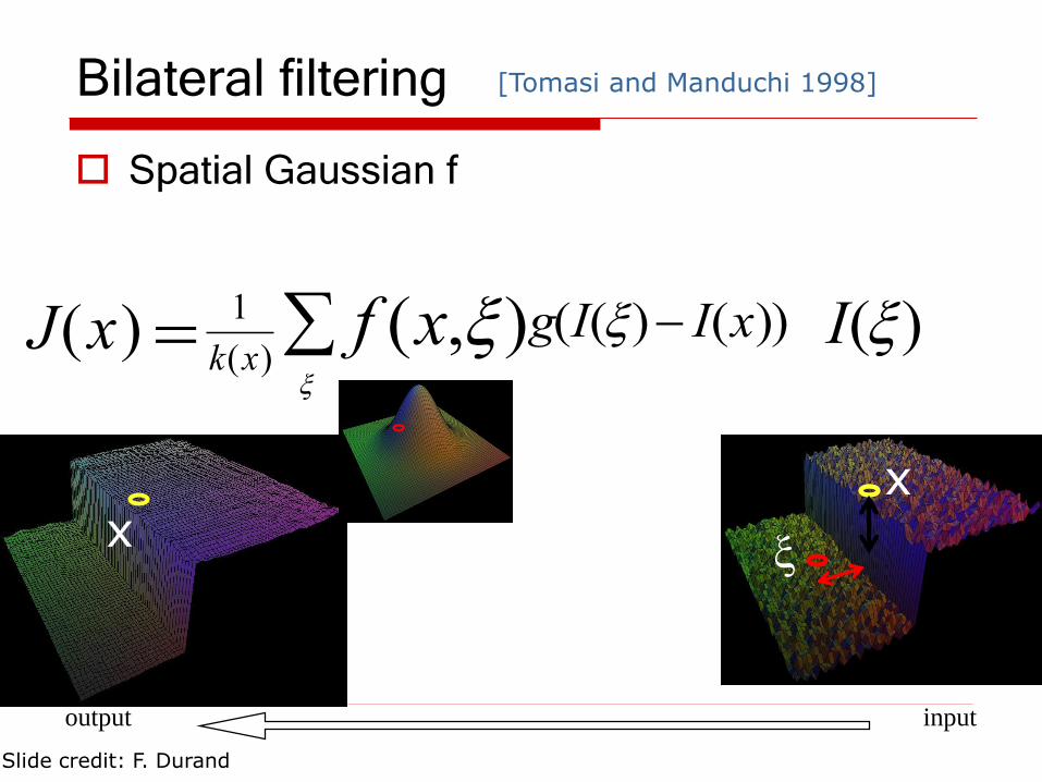
Bilateral filtering

Spatial Gaussian f

output input

J(x)

=

1

k(x)

x

f (x,x)

g(I(x)− I(x))

I(x)

x x

x

Slide credit: F. Durand

[Tomasi and Manduchi 1998]

Bilateral filtering

Spatial Gaussian f

Gaussian g on the intensity difference

output input

J(x)

=

1

k(x)

x

f (x,x)

g(I(x)− I(x))

I(x)

x (x)

I(x)

Slide credit: F. Durand

[Tomasi and Manduchi 1998]

Normalization factor

k(x)=

output input

J(x)

=

1

k(x)

x

f (x,x)

g(I(x)− I(x))

I(x)

x

f (x,x)

g(I(x)− I(x))

[Tomasi and Manduchi 1998]

Slide credit: F. Durand

*

*

*

input output

Same Gaussian kernel everywhere.

Slide credit: P. Sylvain

Blur comes from averaging across edges

*

*

*

input output

The kernel shape depends on the image content.

Slide credit: P. Sylvain

Bilateral filter: no averaging across edges

ss = 2

ss = 6

ss = 18

sr = 0.1 sr = 0.25sr =

(Gaussian blur)

input

Slide credit: P. Sylvain

Parameter for spatial distance Gaussian f

Parameter for intensity difference Gaussian g

ss = 2

ss = 6

ss = 18

sr = 0.1 sr = 0.25sr =

(Gaussian blur)

input

Slide credit: P. Sylvain

Parameter for spatial distance Gaussian f

Parameter for intensity difference Gaussian g

Result

19

Input Output

Reprint from Tomasi and Manduchi 1998

Why do we say it is non-linear?

It does not respect bila(f+g)=bila(f)+bila(g)

Slide credit: F. Durand

Bilateral filtering is non-linear

The weights are different for each output pixel

output input

J(x)

=

1

k(x)

x

f (x,x)

g(I(x)− I(x))

I(x)

x’ x’

Slide credit: F. Durand

Other view

The bilateral filter uses the 3D distance

Slide credit: F. Durand

Speed

Direct bilateral filtering is slow (minutes)

Accelerations exist:

◼ Subsampling in space & range

Durand & Dorsey 2002

Paris & Durand 2006

◼ Limit to box kernel & intelligent maintenance of

histogram

Weiss 2006

Slide credit: F. Durand

LM Filter Bank

Code for filter banks: www.robots.ox.ac.uk/~vgg/research/texclass/filters.html

Slide credit: C. Dyer

Application: Filter Banks for Feature Detection

Filter Banks

Process image with each filter and keep responses (or

squared/abs responses)

Slide credit: C. Dyer

Application: Hybrid Images

http://www.cs.illinois.edu/class/fa10/cs498dwh/projects/hybrid/ComputationalPhotography_ProjectHybrid.html

Gaussian Filter

Laplacian Filter

Project Instructions:

A. Oliva, A. Torralba, P.G. Schyns,

“Hybrid Images,” SIGGRAPH 2006

Gaussianunit impulse Laplacian of Gaussian

I1

I2

G1

(1-G2)

I1 G1

Slide credit: C. Dyer

Slide credit: C. Dyer

Feature detection

◼ Edge

◼ Corner

◼ Blob

29

Edge detection

❑ Goal: Identify sudden changes

(discontinuities) in an image

❑ Intuitively, most semantic and

shape information from the image

can be encoded in the edges

❑ More compact than pixels

❑ Ideal: artist’s line drawing (but

artist is also using object-level

knowledge)

Source: D. Lowe

Origin of edges

Edges are caused by a variety of factors:

depth discontinuity

surface color discontinuity

illumination discontinuity

surface normal discontinuity

Source: Steve Seitz

Characterizing edges

An edge is a place of rapid change in the image

intensity function

imageintensity function

(along horizontal scan line) first derivative

edges correspond toextrema of derivative

Source: S. Lazebnik

For 2D function f(x,y), the partial derivative is:

For discrete data, we can approximate using finite differences:

To implement above as convolution, what would be the

associated filter?

),(),(lim

),(

0

yxfyxf

x

yxf −+=

→

1

),(),1(),( yxfyxf

x

yxf −+

Source: K. Grauman

Derivatives with convolution

Which shows changes with respect to x?

-1

1

1

-1or-1 1

x

yxf

),(

y

yxf

),(

Source: S. Lazebnik

Partial derivatives of an image

Finite difference filters

Other approximations of derivative filters exist:

Source: K. Grauman

The gradient points in the direction of most rapid increase in intensity

Image gradient

The gradient of an image:

The gradient direction is given by

Source: Steve Seitz

The edge strength is given by the gradient magnitude

• How does this direction relate to the direction of the edge?

Effects of noise

Consider a single row or column of the image

◼ Plotting intensity as a function of position gives a signal

Where is the edge?

Source: S. Seitz

Solution: smooth first

To find edges, look for peaks in )( gfdx

d

f

g

f * g

)( gfdx

d

Source: S. Seitz

• Differentiation is convolution, and convolution is

associative:

• This saves us one operation:

gdx

dfgf

dx

d= )(

Derivative theorem of convolution

gdx

df

f

gdx

d

Source: S. Seitz

Derivative of Gaussian filter

Are these filters separable?

x-direction y-direction

Source: S. Lazebnik

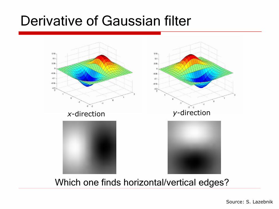
Derivative of Gaussian filter

Which one finds horizontal/vertical edges?

x-direction y-direction

Source: S. Lazebnik

Smoothed derivative removes noise, but blurs

edge. Also finds edges at different “scales”

1 pixel 3 pixels 7 pixels

Scale of Gaussian derivative filter

Source: D. Forsyth

Smoothing filters◼ Gaussian: remove “high-frequency” components;

“low-pass” filter

◼ Can the values of a smoothing filter be negative?

◼ What should the values sum to?

One: constant regions are not affected by the filter

Derivative filters◼ Derivatives of Gaussian

◼ Can the values of a derivative filter be negative?

◼ What should the values sum to?

Zero: no response in constant regions

◼ High absolute value at points of high contrast

Source: K. Grauman and S. Lazebnik

Review: smoothing vs. derivative filters

The Canny edge detector

original image

Slide credit: Steve Seitz

The Canny edge detector

norm of the gradient

Slide credit: Steve Seitz

The Canny edge detector

thresholding

Slide credit: Steve Seitz

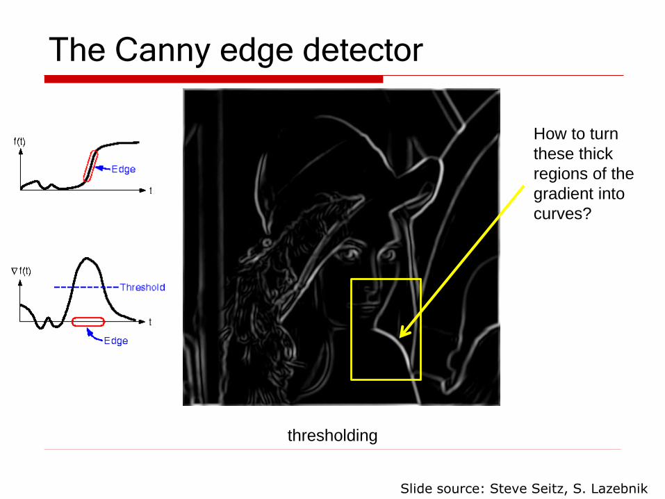
The Canny edge detector

thresholding

How to turn

these thick

regions of the

gradient into

curves?

Slide source: Steve Seitz, S. Lazebnik

Non-maximum suppression

Check if pixel is local maximum along gradient direction,

select single max across width of the edge

◼ requires checking interpolated pixels p and r

Slide source: Steve Seitz, S. Lazebnik

The Canny edge detector

Thinning

(non-maximum suppression)

Problem:

pixels along

this edge

didn’t

survive the

thresholding

Slide source: Steve Seitz, S. Lazebnik

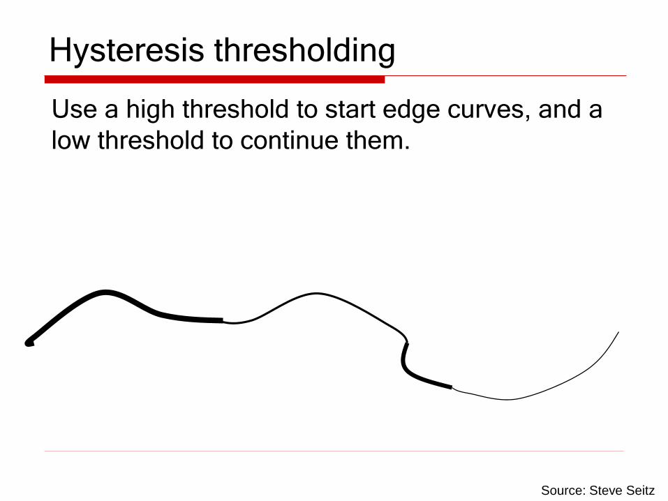
Use a high threshold to start edge curves, and a

low threshold to continue them.

Source: Steve Seitz

Hysteresis thresholding

original image

high threshold

(strong edges)

low threshold

(weak edges)hysteresis threshold

Source: L. Fei-Fei

Hysteresis thresholding

1. Filter image with derivative of Gaussian

2. Find magnitude and orientation of gradient

3. Non-maximum suppression:

◼ Thin wide “ridges” down to single pixel width

4. Linking and thresholding (hysteresis):

◼ Define two thresholds: low and high

◼ Use the high threshold to start edge curves and

the low threshold to continue them

J. Canny, A Computational Approach To Edge Detection, IEEE Trans. Pattern Analysis and Machine Intelligence, 8:679-714, 1986.

Source: D. Lowe, L. Fei-Fei

Recap: Canny edge detector

Next Time

More feature detection

◼ Corner and blob

53