Introduction to ValuationBond Valuation

Financial Management

P.V. Viswanath

For a First course in Finance

P.V. Viswanath 2

Lesson Objectives

To look at the difference between economics and finance

To introduce the notion of future dollars as traded goods.

To introduce the price of future dollars To relate the price of money to interest rates. To use these rates to price Treasury securities To introduce the notion of arbitrage

P.V. Viswanath 3

Absolute and Relative Pricing

In economics, we tend to price goods and assets by considering the factors affecting the supply and demand for them.

The number of goods and assets are very many. Each of them is different in some way or another from the other.

Computing the price of one good does not allow us to price another good, except to the extent that other goods are substitutes or complements for the first good.

In finance, the number of assets can be reasonably characterized in terms of a smaller number of basic characteristics.

Hence most assets can, to a first approximation be priced by considering them as combinations of more fundamental assets.

P.V. Viswanath 4

The Fundamentals of Economics

One of the issues that economics analyzes is the determination of prices of goods.

For example, what determines the price of eggs? We have a supply curve – that is, a schedule of

quantities of eggs that their current possessors would be willing to sell and the prices at which they would be willing to sell them.

The higher the price, the more they’d be willing to sell.

P.V. Viswanath 5

The Supply Curve

Quantity of Eggs

SPrice

($ per unit)

P.V. Viswanath 6

The Demand Curve

We can also imagine the different amounts of eggs that people would be willing to buy and the prices at which they would buy those quantities.

The lower the price, the more would be demanded.

P.V. Viswanath 7

The Demand Curve

Quantity of Eggs

D

Price($ per unit)

P.V. Viswanath 8

The Determination of the Price of Eggs

Quantity of Eggs

D

S

The curves intersect atequilibrium, or market-

clearing, price. At P0 thequantity supplied is equalto the quantity demanded

at Q0 .

P0

Q0

Price($ per unit)

P.V. Viswanath 9

Economics and Finance

Finance, like Economics, is interested in the prices of goods.

But the goods that financial analysts are interested in, are quite different.

As you might imagine, financial economists are interested in money (or purchasing power) and in the price of money.

But what does it mean to talk about the price of money? In what currency would you pay to acquire money?

P.V. Viswanath 10

Money and Time

The answer is that access to resources today is not the same as access to resources tomorrow – that is, money available today is not the same as money available tomorrow.

You can buy something today only if you have the money to buy it with today. Having access to money, which will be available tomorrow won’t allow you to necessarily buy things today!

This means that we can talk of different kinds of money. And, denoting time by the subscript t, we can talk of the

price of time 1 (tomorrow) money in terms of time 0 (today) money.

P.V. Viswanath 11

More on the price of money

Let’s assume that all prices are denominated in t=0 dollars (today’s money).

Then, just as we might say that the price of a book is $10, the price of a subway token is $2 and the price of a cup of Starbucks coffee is $3.50, we could also say

The price of a t=1 dollar is $0.90, the price of a t=2 dollar is $0.7831 and the price of a t=3 dollar is $0.675.

P.V. Viswanath 12

The price of coffee, said differently

This might sound a little strange to you, but let’s put it slightly differently.

Going back to a cup of coffee, we said its price was $3.50, but if we know that $3.50 = €1, we could equally well say that the price of a book is €1.

Then even if we were all in the US and Starbucks only accepted US dollars, there would be no problem if Starbucks had its price list denominated in euros.

P.V. Viswanath 13

More ways to price coffee

Let’s take this further. Suppose Starbucks required everybody to play the following

game in order to figure out the price of its offering. Suppose they took the actual dollar price of a coffee

multiplied it by 2 and added 3 to it and called it java units (J). A cup of coffee that normally cost $3.5 would be listed as

costing 10J. Then if we saw a cappuccino listed at 13J, we would simply

subtract 3 to get 10, then divide by 2 to get a price of $5. It would be a little weird, but nothing substantive would

change.

P.V. Viswanath 14

Rates

So now, let’s go back to the price of money: we said that the price of a t=1 dollar was $0.90, and that the price of a t=2 dollar was $0.7831.

Now clearly the price of a t=1 dollar, which is $0.90 today, will rise to $1 at t=1.

Hence providing today’s price of a t=1 dollar is equivalent to providing the rate of change of the price over the coming period.

I have exactly the same information in each case. This rate of change is also my rate of return over the next

year if I buy a t=1 dollar, today, and is also known as the interest rate.

In our example, this works out to (1-0.90)/0.90 or 11.11%

P.V. Viswanath 15

Rates

What about the price of a t=2 dollar, which we said was $0.7831?

Once again, the price of this t=2 dollar would be $1 at t=2 (in t=2 dollars, of course).

We could compute the gross return on this investment, in the same way, as 1/0.7831 = 1.277 or a return of 27.70%.

But this is a return over two periods, and we cannot compare it directly to the 11.11% that we computed earlier.

The solution to this problem is to annualize the two-period return

P.V. Viswanath 16

Computing Annualized Rates

We computed the return on buying a t=2 dollar at 27.70%. Suppose the one-period return on this is r%; that is, the

return from holding this t=2 dollar from now until t=1 is r%. Then, every dollar invested in this specialized investment could be sold at $(1+r) at t=1.

Now, if we assume the return on this t=2 dollar if held from t=1 to t=2 is also r%, then the $(1+r) value of our outlay of one t=0 dollar in this investment would be $(1+r)(1+r) or (1+r)2.

But we already know from our return computation, that this is exactly 1.277 (that is 1 plus the 27.7%).

Hence we equate (1+r)2 to 1.277 and solve for r.

P.V. Viswanath 17

Annualized Rates

This involves simply taking the square-root of 1.277, which is 13%.

Of course, we won’t get exactly 13% in each of the two periods.

The 13% rate is, rather, a sort of average return over the two periods, that results in a 27.7% over the two years.

We can now take $0.675, the price of a t=3 dollar and also convert it to a rate of return.

In this case, we take the cube root of (1/0.675), which works out 14%

P.V. Viswanath 18

Yield to maturity

So now we have the current prices of t=1, t=2, and t=3 dollars, or $0.90, $0.7831 and $0.675 respectively.

Alternatively, the information in these prices could also be presented as rates of return, which in our case are 11.11%, 13% and 14% respectively.

These rates are also called yields-to-maturity. Yields-to-maturity, in general, are the annualized total

returns that you would get if you held a particular financial instrument to maturity.

In this case, the returns each year are only from price appreciation, while in other cases, there may be annual cash payments received by the investor, as well.

P.V. Viswanath 19

Using the rates

We have assumed, up to this point, that purchasing a t=1 dollar is riskless. That is, the person who sold us the t=1 dollar today, in return for the $0.90, would, in fact, pay us $1 at time t=1.

We will continue with this assumption, for now. Note, as well that buying a t=1 dollar is equivalent to

lending money for one period, while selling a t=1 dollar is equivalent to borrowing money for 1 period.

A bond is precisely a promise to pay its holder some combination of future dollars.

Corporations, governments and other entities who need funds for the continuing operations issue, that is sell, such bonds.

P.V. Viswanath 20

Treasury Bonds

Consider now a bond issued by the Treasury Department, which essentially acts as banker for the Federal Government.

These bonds, or promises to pay are considered default-free, i.e. we fully expect the Treasury to live up to its promises.

We can, therefore, evaluate and price these Treasury or T-bonds using the “risk-free” yields that we established before.

This need not be true of other governmental institutions, such as municipalities, such as the City of New York or Federal agencies such as PATH – the Port Authority of New York and New Jersey.

P.V. Viswanath 21

Treasury Bonds

On Feb. 29th 2008, the Treasury issued a 2% note with a maturity date of February 28, 2010 with a face value of $1000, which was sold at auction.

The price paid by the lowest bidder was 99.912254% of face value.

This means that the buyer of this bond would get every six months 1% (half of 2%) of the face value, which in this case works out to $10.

In addition, on Feb. 28, 2010, the buyer would get $1000.

P.V. Viswanath 22

Terminology

The maturity of this bond is 2 years. The coupon rate on this bond is 2% The face value of this bond is $1000 The price paid for this bond is $999.123 The yield-to-maturity obtained by this buyer is

2.045%, i.e. the average rate of return for this buyer if s/he held it to maturity.

P.V. Viswanath 23

Pricing this bond

Let’s assume for now, that we do not know the price of this bond. How can we price this bond?

What we do know is that a holder of this bond would receive $10 in 6 months, another $10 in 1 year, $10 again in 1.5 years and $1010 in 2 years.

We also know that a 6-month T-bill issued on Feb. 21, 2008 sold for 98.968667.

A T-bill is a promise to pay money 6 months in the future. With the given price then, a buyer would get a 1.042% return for those 6 months.

This is often annualized by multiplying by 2 to get a bond-equivalent yield of 2.084%.

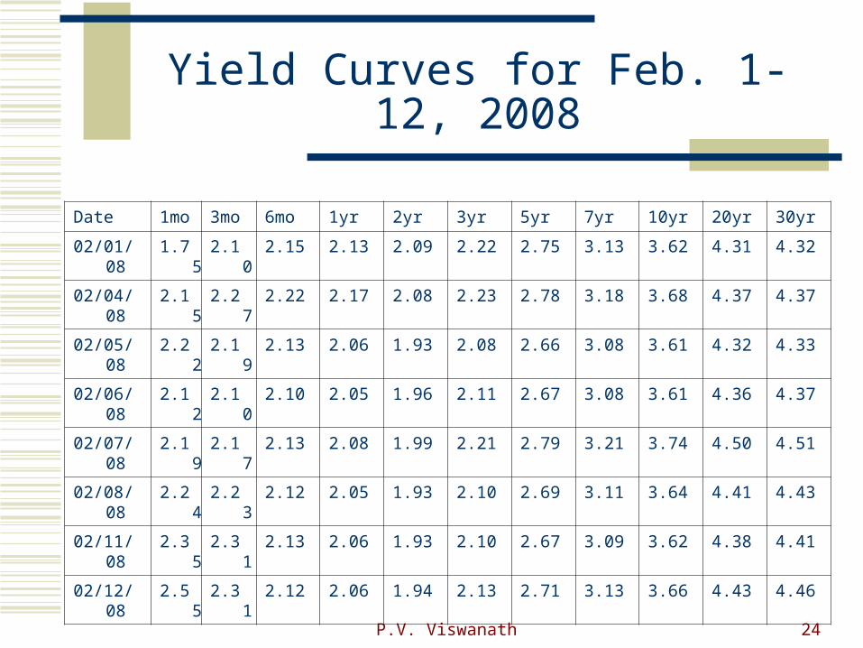
We also know that yields of bonds generally are higher for higher maturities.

P.V. Viswanath 24

Yield Curves for Feb. 1-12, 2008

Date 1mo 3mo 6mo 1yr 2yr 3yr 5yr 7yr 10yr 20yr 30yr

02/01/08 1.75 2.10 2.15 2.13 2.09 2.22 2.75 3.13 3.62 4.31 4.32

02/04/08 2.15 2.27 2.22 2.17 2.08 2.23 2.78 3.18 3.68 4.37 4.37

02/05/08 2.22 2.19 2.13 2.06 1.93 2.08 2.66 3.08 3.61 4.32 4.33

02/06/08 2.12 2.10 2.10 2.05 1.96 2.11 2.67 3.08 3.61 4.36 4.37

02/07/08 2.19 2.17 2.13 2.08 1.99 2.21 2.79 3.21 3.74 4.50 4.51

02/08/08 2.24 2.23 2.12 2.05 1.93 2.10 2.69 3.11 3.64 4.41 4.43

02/11/08 2.35 2.31 2.13 2.06 1.93 2.10 2.67 3.09 3.62 4.38 4.41

02/12/08 2.55 2.31 2.12 2.06 1.94 2.13 2.71 3.13 3.66 4.43 4.46

P.V. Viswanath 25

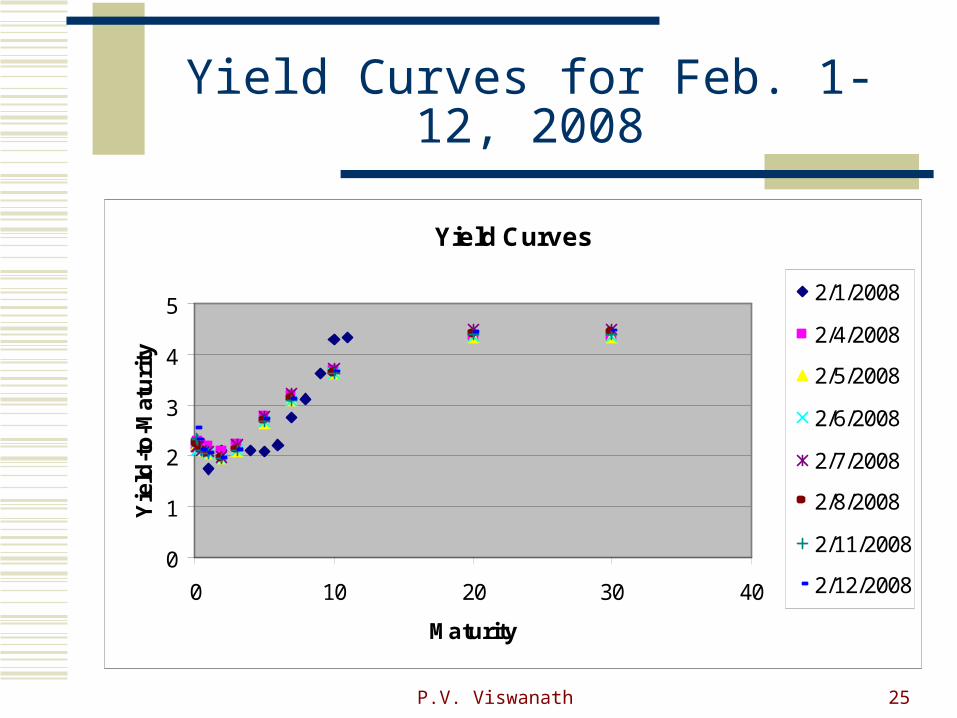
Yield Curves for Feb. 1-12, 2008

Yield Curves

0

1

2

3

4

5

0 10 20 30 40

Maturity

Yie

ld-t

o-M

atu

rity

2/1/2008

2/4/2008

2/5/2008

2/6/2008

2/7/2008

2/8/2008

2/11/2008

2/12/2008

P.V. Viswanath 26

Pricing a Treasury bond

Suppose we believe that the current environment of uncertainty will continue.

We might believe that investors will be even more unwilling to invest in securities that have any default risk.

In that case, they will be willing to buy Treasury securities at lower yields.

We use this to estimate current bond-equivalent yields. Suppose we estimate the current bond-equivalent yields for

6-month money, 1 year money, 18-month money and 2 year money as 2.07%, 2.1%, 2.11% and 2.14%.

P.V. Viswanath 27

Discounting

Keeping in mind that what we have are bond-equivalent yields, i.e. yields computed on a six-monthly basis and then doubling to get the annual yield, we will compute the current prices of future dollars.

To do this, we need to employ a procedure called discounting.

Suppose the required risk-free rate of return on future dollars is 4% per period.

Now, if I have a certain, default-free promise of $200 in 3 periods, what is the value of this promise today?

P.V. Viswanath 28

Discounting

We know the value at t=3 of this promise would be exactly 200.

The value at t=2of the promise would have to be such that would yield a return of exactly 4% over the last period, i.e. from t=2 to t=4.

Suppose the required value is $S. Then, we would need (200-S)/S = 1.04.

Solving this equation, we find S = 200/1.04. What would the value at t=1 be? Applying the same principle, we see that it must be S/1.04

or 200/1.042. Analogously, we can see that the value at t=0 of a promise

to pay $200 in n periods is 200/(1.04)n.

P.V. Viswanath 29

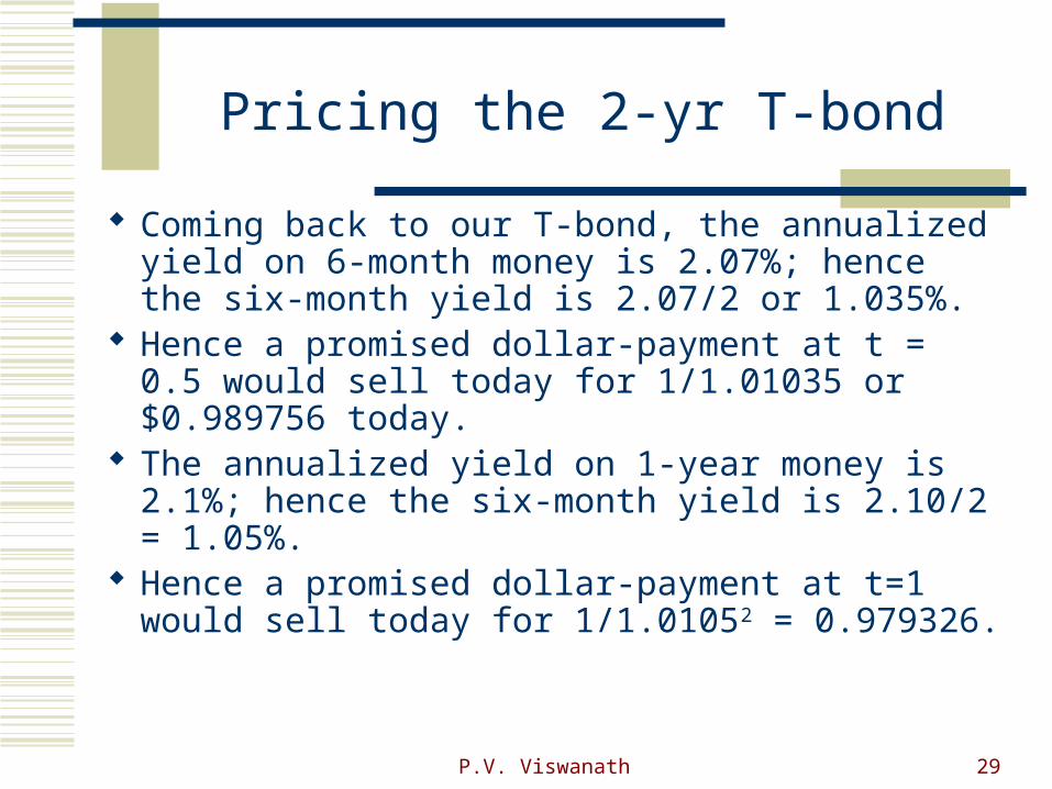
Pricing the 2-yr T-bond

Coming back to our T-bond, the annualized yield on 6-month money is 2.07%; hence the six-month yield is 2.07/2 or 1.035%.

Hence a promised dollar-payment at t = 0.5 would sell today for 1/1.01035 or $0.989756 today.

The annualized yield on 1-year money is 2.1%; hence the six-month yield is 2.10/2 = 1.05%.

Hence a promised dollar-payment at t=1 would sell today for 1/1.01052 = 0.979326.

P.V. Viswanath 30

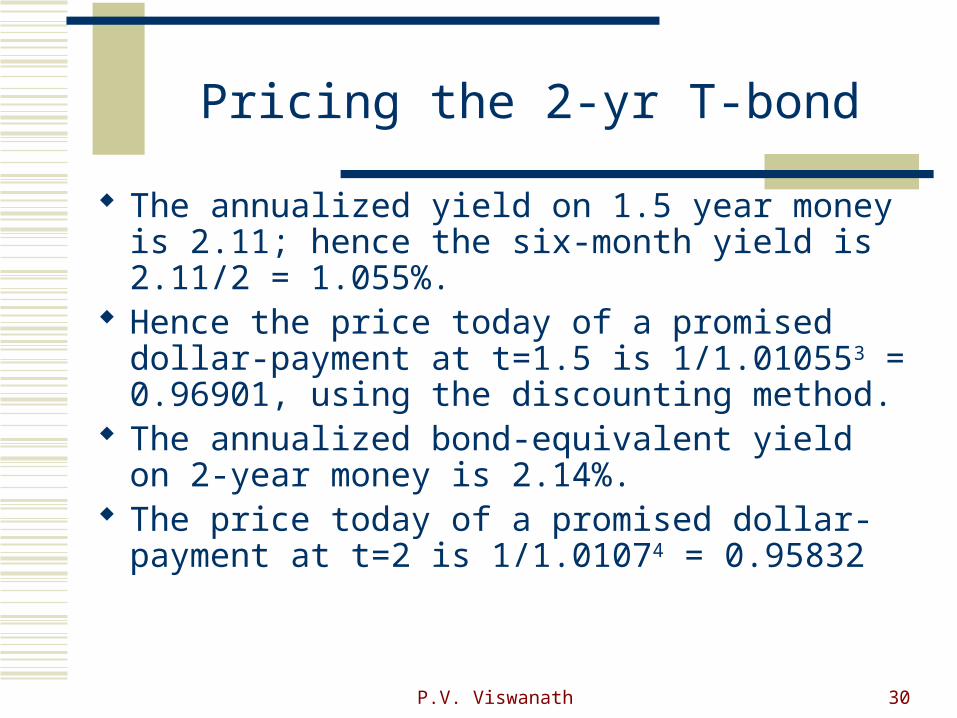
Pricing the 2-yr T-bond

The annualized yield on 1.5 year money is 2.11; hence the six-month yield is 2.11/2 = 1.055%.

Hence the price today of a promised dollar-payment at t=1.5 is 1/1.010553 = 0.96901, using the discounting method.

The annualized bond-equivalent yield on 2-year money is 2.14%.

The price today of a promised dollar-payment at t=2 is 1/1.01074 = 0.95832

P.V. Viswanath 31

Pricing the 2-yr T-bond

So now we know that our bond pays $10 in 6 months, another $10 in 1 year, $10 again in 1.5 years and $1010 in 2 years.

We also know that one dollar promised for each of those dates is worth, today, $0.989756, $ 0.979326, $ 0.96901 and $ 0.95832 respectively.

Our bond, therefore, must sell for 10(0.989756) + 10(0.979326) + 10(0.96901) + 1010(0.95832) = $997.28.

P.V. Viswanath 32

Arbitrage

What we have done is to treat our 2 year 2% coupon bond as a portfolio of four other zero-coupon bonds and then priced it as the sum of the values of those zero-coupon bonds.

But what will guarantee that this price equality will hold? Here’s where the efficient functioning of markets comes

into play. A process called arbitrage ensures that the price of a

combination of other financial securities does not deviate too much from the price implied the prices of those other securities.

P.V. Viswanath 33

Arbitrage

Suppose, for example that our two-year bond sold for $996.

Then a bond trader could buy a bond at this price, then, himself, issue the corresponding four zero-coupon bonds and sell them at their market prices.

He would then end up with a profit of $1.28 per bond.

If the bond sold for, say, $998, he could buy the zero-coupon bonds and then create a “synthetic” coupon bond and sell it at the higher price and make a profit of 998-997.28 or 72 cents per bond.

P.V. Viswanath 34

Relative pricing of financial assets

Consider first riskless financial assets, i.e, assets that are claims on riskless cashflows over time.

Consider a fundamental asset, i, defined by a claim to $1 at time t = i. There can be T such fundamental assets, corresponding to the t = 1,..,T

time units. Then, any arbitrary riskless financial asset that is a claim to $ci at time i,

i = 1,..,T can be considered a portfolio of these T fundamental assets. Hence, the price, P* of any such asset is related to the prices of these first

T fundamental assets. In fact, the price of this asset would simply be

T

iii PcP

1

*

P.V. Viswanath 35

Relative pricing of risky financial assets

What about risky financial assets? We can equivalently imagine, for every level of risk, a set of T

fundamental risky assets. Then, for any arbitrary risky asset of this level of risk, we can equivalently write:

T

iii PcP

1

*

Of course, this is not entirely satisfactory, because we’d have TxM fundamental assets corresponding to each of M levels of risk. We will come back to this when we talk about the CAPM.

In any case, we need to examine how this pricing is established in the market-place.

P.V. Viswanath 36

Arbitrage and the Law of One Price

Law of One Price: In a competitive market, if two assets generate the same cash (utility) flows, they will be priced the same.

How is this enforced? If the law is violated – if asset 1 sells for more than asset 2,

then investors can make a riskless profit by buying asset 2 and selling it as asset 1!

In practice – we need to take transactions costs into account. Also, it may be difficult to execute the two transactions at

the same time – prices might change in that interval – this introduces some risk.

P.V. Viswanath 37

Exchange Rates and Triangular Arbitrage

Consider the exchange rates reigning at closing on January 30. The yen/euro rate was 157.87 yen per euro The euro/$ rate was $1.4835 per euro. The yen/$ rate was 106.4 yen per dollar.

If we start with a dollar, we can buy 106.4 yen; these can then be used to buy 106.4/157.87 or 0.674 euros, which can, in turn, be used to acquire $0.9998, which is very close to a dollar.

P.V. Viswanath 38

Triangular Currency Arbitrage

Suppose the euro/$ rate had been $1.50 per euro. Then, it would have been possible to start with one dollar,

acquire 0.674 euros, as above, and then get (0.674)(1.5) or $1.011, or a gain of 1.1% on the initial investment of a dollar.

This would imply that the dollar was too cheap, relative to the euro and the yen.

Many traders would attempt to perform the arbitrage discussed above, leading to excess supply of dollars and excess demand for the other currencies.

The net result would be a drop a rise in the price of the dollar vis-à-vis the other currencies, so that the arbitrage trades would no longer be profitable.

P.V. Viswanath 39

Risk Arbitrage

In this case, trading will continue until there are no more riskfree profit opportunities.

Thus, arbitrage can ensure that the sorts of pricing relationships referred to above can be supported in the marketplace, viz:

T

iii PcP

1

*

What if there are still opportunities that will, on average, lead to profit, but the investors intending to benefit from this profit will have to take on some risk?

Presumably investors will trade off the risk against the expected profit so that there will be few of these expected profit opportunities, as well; this brings us to the notion of the informational efficiency of financial markets.

P.V. Viswanath 40

Efficient Markets Hypothesis – EMH

An asset’s current price reflects all available information– this is the EMH.

If it didn’t, there would be an incentive for investors to act on that information.

Suppose, for example, that investors noticed that good news led to stock prices rising slowly over two consecutive days.

This would mean that at the end of the first day, the good news was not all incorporated in the stock price.

P.V. Viswanath 41

Efficient Markets Hypothesis

In this situation, it would be optimal for traders to buy even more of a stock that was noted to be rising on a given day, since the stock would rise more the next day, giving the trader an unusually good chance of making money on the trade.

But if many traders pursue this strategy, the stock price would rise on the first day, itself, and the informational inefficiency would be eliminated.

Empirically, financial markets seem to be reasonably close to being efficient.

This allows us to price financial assets with respect to fundamentals without worrying about deviations from these fundamental prices.

P.V. Viswanath 42

Stock Price Fundamentals

What determines the price of a stock? Or, in other words, why would an investor hold stocks?

The answer is that s/he expects to receive dividends and hopefully benefit from a price increase, as well.

In other words, P0 = PV(D1) + PV(P1) However what determines P1? Again, using the previous logic, we must say that

it’s the expectation of a dividend in period 2 and hopefully a further price rise. Continuing, in this vein, we see that the stock price must be the sum of the present values of all future dividends.

P.V. Viswanath 43

Dividend Mechanics

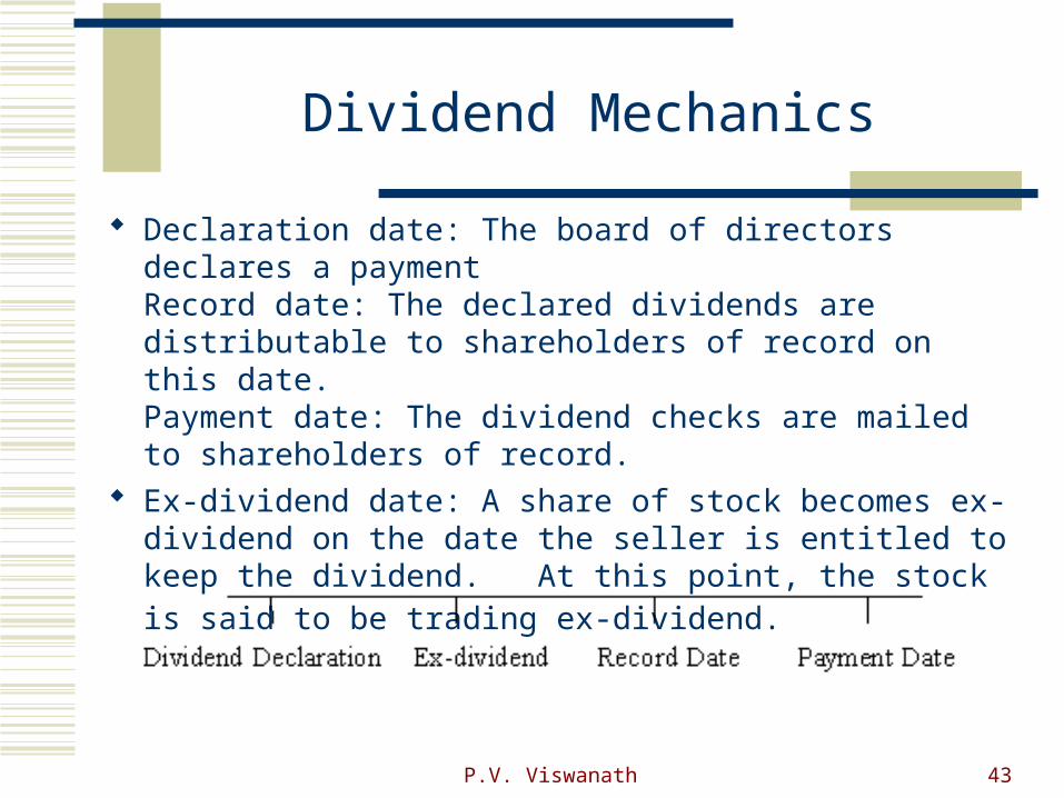
Declaration date: The board of directors declares a paymentRecord date: The declared dividends are distributable to shareholders of record on this date.Payment date: The dividend checks are mailed to shareholders of record.

Ex-dividend date: A share of stock becomes ex-dividend on the date the seller is entitled to keep the dividend.   At this point, the stock is said to be trading ex-dividend. 

P.V. Viswanath 44

Dividend Discount Model

What is the price of a stock on its ex-dividend date? Using the previous logic, we see that it’s simply

...)1(

...)1(1 2

210

nk

Dn

k

D

k

DP

where k is the appropriate discount rate to discount the dividends consistent with their riskiness.

We assume that the one-period ahead discount rate is the same for all periods. That is, we use the same rate to discount D1 to time 0, as we use to discount D2 to time 1.

P.V. Viswanath 45

Gordon Growth Model

If we assume that the dividend is growing at a rate of g% per annum forever, this formula simplifies to:

gk

DP

1

0

We see that the price of a stock is higher, the higher the level of dividends, the higher the growth rate of dividends and the lower the required rate of return or the discount rate, k.

P.V. Viswanath 46

Two essential concepts

1. Cash flows at different points in time cannot be compared and aggregated. All cash flows have to be brought to the same point in time, before comparisons and aggregations are made.

2. The concept of a Time Line:

0 1 2 3

4$ 100 $ 100 $ 100$ 100

Figure 3.1: A Time Line for Cash Flows: $ 100 in Cash Flows Received at the End of Each of Next 4 years

Cash Flows

Year

P.V. Viswanath 47

Cash Flow Types and Discounting Mechanics

There are five types of cash flows - simple cash flows, annuities, growing annuities perpetuities and growing perpetuities

P.V. Viswanath 48

I. Simple Cash Flows

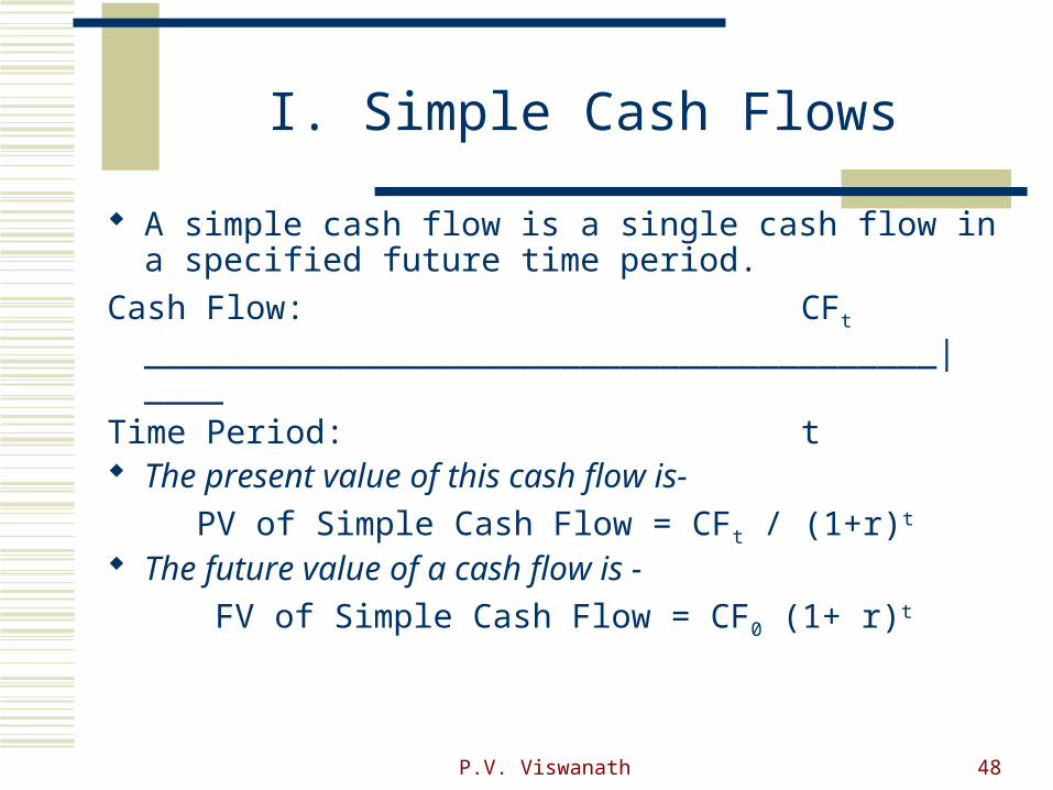
A simple cash flow is a single cash flow in a specified future time period.

Cash Flow: CFt

________________________________________|____Time Period: t The present value of this cash flow is-

PV of Simple Cash Flow = CFt / (1+r)t

The future value of a cash flow is -

FV of Simple Cash Flow = CF0 (1+ r)t

P.V. Viswanath 49

Application: The power of compounding - Stocks, Bonds and

Bills Between 1926 and 1998, Ibbotson Associates found

that stocks on the average made about 11% a year, while government bonds on average made about 5% a year.

If your holding period is one year,the difference in end-of-period values is small: Value of $ 100 invested in stocks in one year = $ 111 Value of $ 100 invested in bonds in one year = $ 105

P.V. Viswanath 50

Holding Period and Value

Figure 3.3: Effect of Compounding Periods: Stocks versus T.Bonds

$0.00

$1,000.00

$2,000.00

$3,000.00

$4,000.00

$5,000.00

$6,000.00

$7,000.00

Compounding Periods

StocksT. Bonds

$ 100 invested in stocks, earning 11% a year, is worth more than seen times as much at the end of 40 years than $ 100 invested in bonds, earning 5% a year.

The compounding effect increasesas the time horizon increases.

P.V. Viswanath 51

The Frequency of Compounding

The frequency of compounding affects the future and present values of cash flows. The stated interest rate can deviate significantly from the true interest rate – For instance, a 10% annual interest rate, if there is

semiannual compounding, works out to-Effective Interest Rate = 1.052 - 1 = .10125 or 10.25%

The general formula isEffective Annualized Rate = (1+r/m)m – 1where m is the frequency of compounding (# times per year), andr is the stated interest rate (or annualized percentage rate (APR) per year

P.V. Viswanath 52

The Frequency of Compounding

Frequency Rate t FormulaEffective Annual Rate

Annual 10% 1 r 10.00%

Semi-Annual 10% 2 (1+r/2)2-1 10.25%

Monthly 10% 12 (1+r/12)12-1 10.47%

Daily 10% 365 (1+r/365)365-1 10.52%

Continuous 10%   er-1 10.52%

P.V. Viswanath 53

II. Annuities

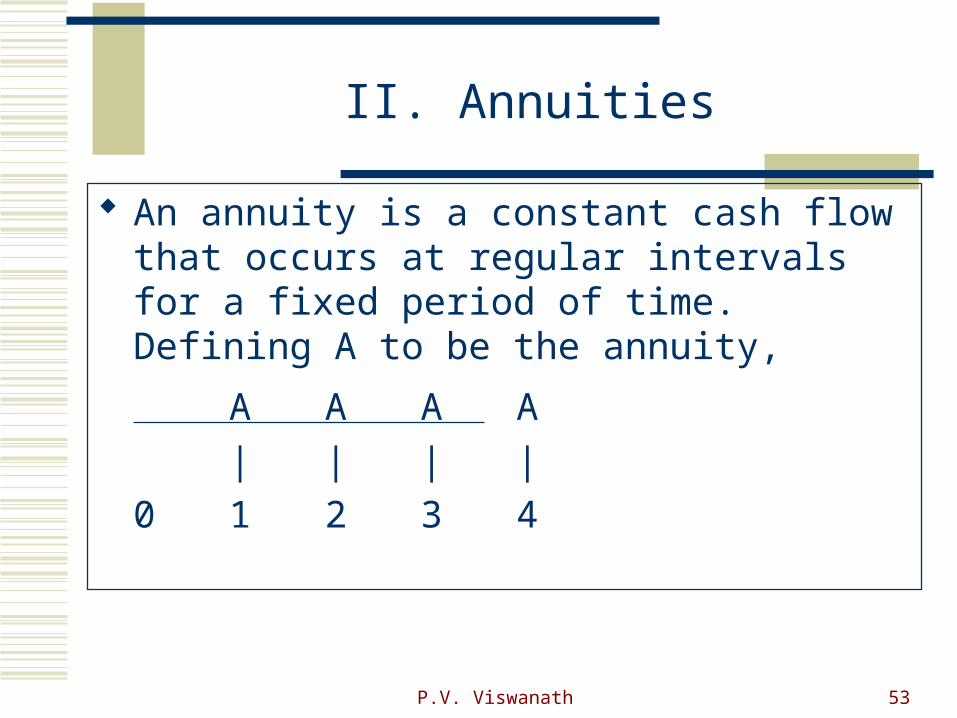
An annuity is a constant cash flow that occurs at regular intervals for a fixed period of time. Defining A to be the annuity,

A A A A

| | | |

0 1 2 3 4

P.V. Viswanath 54

Present Value of an Annuity

The present value of an annuity can be calculated by taking each cash flow and discounting it back to the present, and adding up the present values. Alternatively, there is a short cut that can be used in the calculation [A = Annuity; r = Discount Rate; n = Number of years]

nrr

AnrAPVAnnuityanofPV

)1(

11),,(

P.V. Viswanath 55

Example: PV of an Annuity

The present value of an annuity of $1,000 at the end of each year for the next five years, assuming a discount rate of 10% is -

The notation that will be used in the rest of these lecture notes for the present value of an annuity will be PV(A,r,n).

PV of $1000 each year for next 5 years = $1000

1 - 1

(1.10)5

.10

$3,791

P.V. Viswanath 56

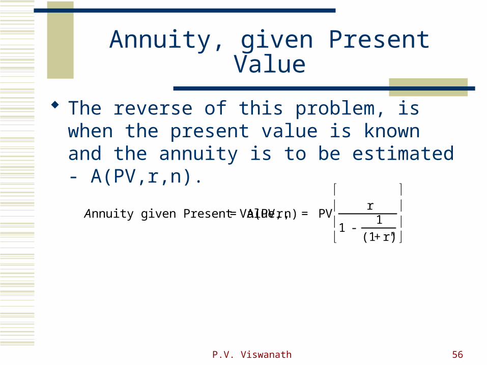
Annuity, given Present Value

The reverse of this problem, is when the present value is known and the annuity is to be estimated - A(PV,r,n).

Annuity given Present Value = A(PV, r,n) = PV r

1 - 1

(1 + r)n

P.V. Viswanath 57

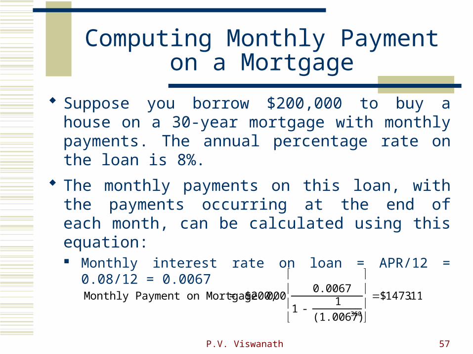
Computing Monthly Payment on a Mortgage

Suppose you borrow $200,000 to buy a house on a 30-year mortgage with monthly payments. The annual percentage rate on the loan is 8%.

The monthly payments on this loan, with the payments occurring at the end of each month, can be calculated using this equation: Monthly interest rate on loan = APR/12 = 0.08/12 =

0.0067

Monthly Payment on Mortgage = $200,000 0.0067

1 - 1

(1.0067)360

$1473.11

P.V. Viswanath 58

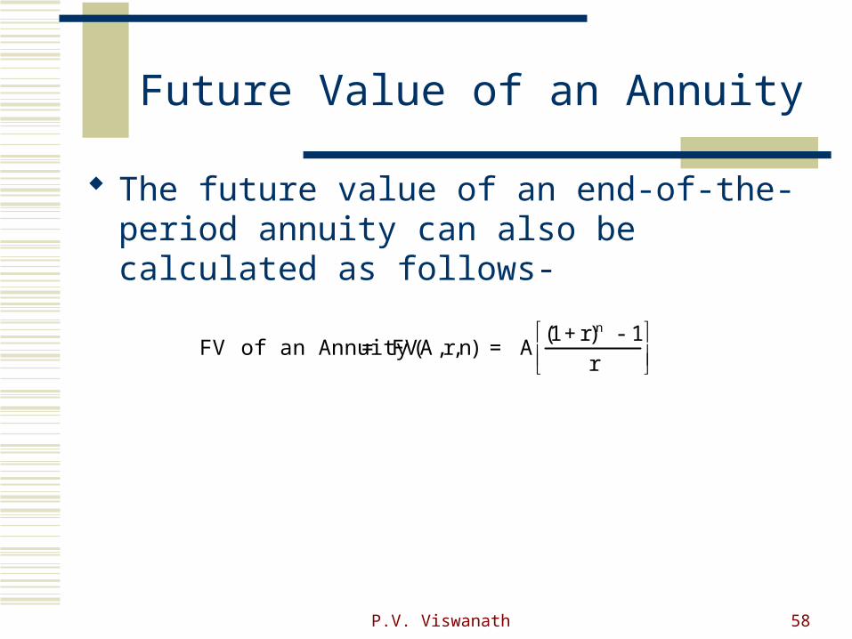
Future Value of an Annuity

The future value of an end-of-the-period annuity can also be calculated as follows-

FV of an Annuity = FV(A,r,n) = A (1 + r)n - 1

r

P.V. Viswanath 59

An Example

Thus, the future value of $1,000 at the end of each year for the next five years, at the end of the fifth year is (assuming a 10% discount rate) -

The notation that will be used for the future value of an annuity will be FV(A,r,n).

FV of $1,000 each year for next 5 years = $1000 (1.10)5 - 1

.10

= $6,105

P.V. Viswanath 60

Annuity, given Future Value

If you are given the future value and you are looking for an annuity - A(FV,r,n) in terms of notation -

Annuity given Future Value = A(FV, r,n) = FV r

(1+ r)n - 1

Note, however, that the two formulas, Annuity, given Future Value and Present Value, given annuity can be derived from each other, quite easily. You may want to simply work with a single formula.

P.V. Viswanath 61

Application : Saving for College Tuition

Assume that you want to send your newborn child to a private college (when he gets to be 18 years old). The tuition costs are $16000/year now and that these costs are expected to rise 5% a year for the next 18 years. Assume that you can invest, after taxes, at 8%.

Expected tuition cost/year 18 years from now = 16000*(1.05)18 = $38,506 PV of four years of tuition costs at $38,506/year = $38,506 * PV(A ,8%,4

years) = $127,537

If you need to set aside a lump sum now, the amount you would need to set aside would be -

Amount one needs to set apart now = $127,357/(1.08)18 = $31,916

If set aside as an annuity each year, starting one year from now - If set apart as an annuity = $127,537 * A(FV,8%,18 years) = $3,405

P.V. Viswanath 62

Valuing a Straight Bond

You are trying to value a straight bond with a fifteen year maturity and a 10.75% coupon rate. The current interest rate on bonds of this risk level is 8.5%.PV of cash flows on bond = 107.50* PV(A,8.5%,15 years) + 1000/1.08515 = $

1186.85 If interest rates rise to 10%,

PV of cash flows on bond = 107.50* PV(A,10%,15 years)+ 1000/1.1015 = $1,057.05

Percentage change in price = -10.94% If interest rate fall to 7%,

PV of cash flows on bond = 107.50* PV(A,7%,15 years)+ 1000/1.0715 = $1,341.55

Percentage change in price = +13.03%

P.V. Viswanath 63

III. Growing Annuity

A growing annuity is a cash flow growing at a constant rate for a specified period of time. If A is the current cash flow, and g is the expected growth rate, the time line for a growing annuity looks as follows –

0 1 2 3

A(1+g)2

Figure 3.8: A Growing Annuity

A(1+g)3 A(1+g)nA(1+g)

n...........

P.V. Viswanath 64

Present Value of a Growing Annuity

The present value of a growing annuity can be estimated in all cases, but one - where the growth rate is equal to the discount rate, using the following model:

In that specific case, the present value is equal to the nominal sums of the annuities over the period, without the growth effect.

PV of an Annuity = PV(A,r,g,n) = A(1 +g) 1 -

(1+g)n

(1+r)n

(r - g)

P.V. Viswanath 65

The Value of a Gold Mine

Consider the example of a gold mine, where you have the rights to the mine for the next 20 years, over which period you plan to extract 5,000 ounces of gold every year. The price per ounce is $300 currently, but it is expected to increase 3% a year. The appropriate discount rate is 10%. The present value of the gold that will be extracted from this mine can be estimated as follows –

PV of extracted gold = $300* 5000 * (1.03)

1 - (1.03)20

(1.10)20

.10 - .03

$16,145,980

P.V. Viswanath 66

IV. Perpetuity

A perpetuity is a constant cash flow at regular intervals forever. The present value of a perpetuity is-

PV of Perpetuity = A

r

P.V. Viswanath 67

Valuing a Consol Bond

A consol bond is a bond that has no maturity and pays a fixed coupon. Assume that you have a 6% coupon console bond. The value of this bond, if the interest rate is 9%, is as follows -

Value of Consol Bond = $60 / .09 = $667

P.V. Viswanath 68

V. Growing Perpetuities

A growing perpetuity is a cash flow that is expected to grow at a constant rate forever. The present value of a growing perpetuity is -

where CF1 is the expected cash flow next year, g is the constant growth rate and r is the discount rate.

PV of Growing Perpetuity = CF1

(r - g)

P.V. Viswanath 69

Valuing a Stock with Growing Dividends

Southwestern Bell paid dividends per share of $2.73 in 1992. Its earnings and dividends have grown at 6% a year between 1988 and 1992, and are expected to grow at the same rate in the long term. The rate of return required by investors on stocks of equivalent risk is 12.23%.

Current Dividends per share = $2.73

Expected Growth Rate in Earnings and Dividends = 6%

Discount Rate = 12.23%

Value of Stock = $2.73 *1.06 / (.1223 -.06) = $46.45

P.V. Viswanath 70

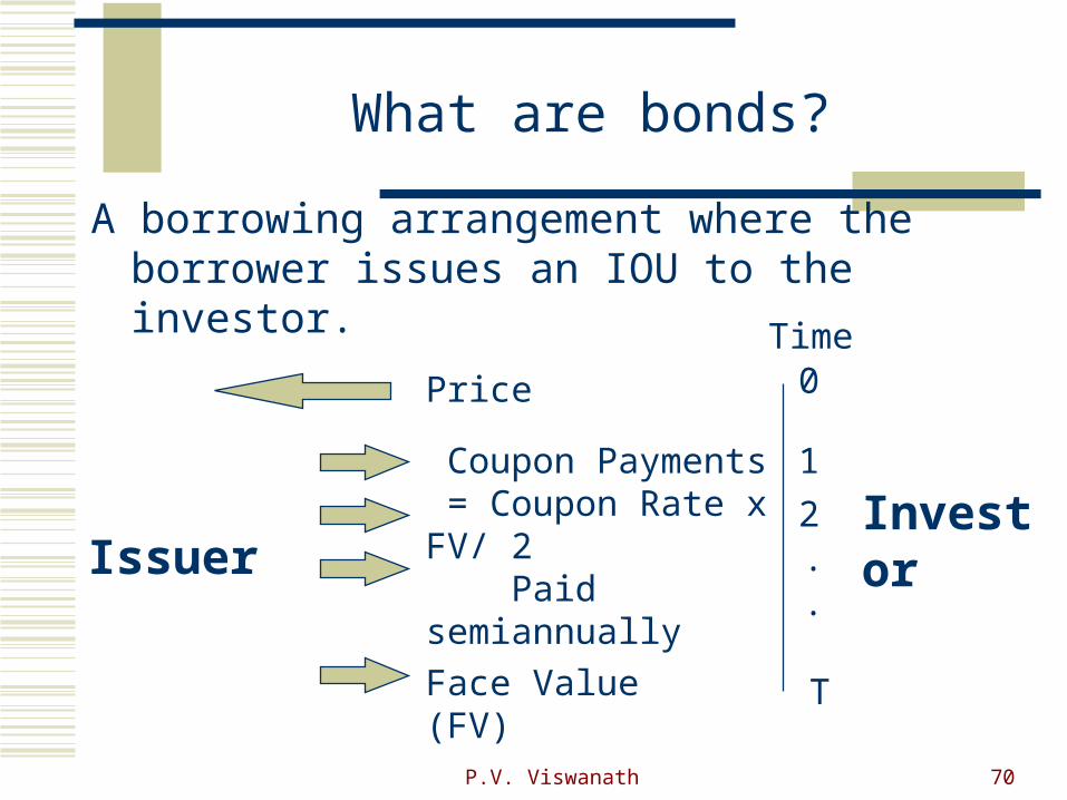
What are bonds?

A borrowing arrangement where the borrower issues an IOU to the investor.

InvestorIssuer

Price 0

TFace Value (FV)

Coupon Payments = Coupon Rate x FV/ 2 Paid semiannually

1

2..

Time

P.V. Viswanath 71

Bond Pricing

A T-period bond with coupon payments of $C per period and a face value of F.

The value of this bond can be computed as the sum of the present value of the annuity component of the bond plus the present value of the FV, where is the present value of an

annuity of $1 per period for T periods, with a discount rate of r% per period.

0 1 2 3 T

0 C C C

4 5

C + FVC C

CAF

rrT

T

( )1

TrA

P.V. Viswanath 72

Bonds with semi-annual coupons

Normally, bonds pay semi-annual coupons:

The bond value is given by:

where the first component is, once again, the present value of an annuity, and y is the bond’s yield-to-maturity.

0 0.5 1 1.5 T

0 C/2

2 2.5

C/2+FC/2 C/2 C/2 C/2

CA

F

yyT

T2 1 222

2/ ( / )

P.V. Viswanath 73

Bond Pricing Example

If F = $100,000; T = 8 years; the coupon rate is 10%, and the bond’s yield-to-maturity is 8.8%, the bond's price is computed as:

= $106,789.52

( . )

. . ( . )

01 100000

2

1

0441

1

1044

16 100000

1044 16 x

P.V. Viswanath 74

The Relation between Bond Prices and Yields

Consider a 2 year, 10% coupon bond with a $1000 face value. If the bond yield is 8.8%, the price is 50 + 1000/(1.044)4 = 1021.58.

Now suppose the market bond yield drops to 7.8%. The market price is now given by 50 + 1000/(1.039)4 = 1040.02.

As the bond yield drops, the bond price rises, and vice-versa.

A.0394

A.0444

P.V. Viswanath 75

Bond Prices and YieldsA Graphic View

Bond Price

Bond Yield

P.V. Viswanath 76

Bond Yield MeasurementDefinitions

Yield to MaturityA measure of the average rate of return on a bond if held to maturity. To compute it, we define the length of a period as 6 months, and then calculate the internal rate of return per period. Finally, we double the six-monthly IRR to get the bond equivalent yield, or yield to maturity. This is more commonly used in the marketplace.

Effective Annual YieldTake the six-monthly IRR and annualize it by compounding. This measure is less commonly used.

P.V. Viswanath 77

Bond Yield Measurement: Examples

An 8% coupon, 30-year bond is selling at $1276.76. First solve the following equation:

This equation is solved by r = 0.03. (You will see later how to solve this equation.)

The yield-to-maturity is given by 2 x 0.03 = 6% The effective annual yield is given by (1.03)2 - 1 = 6.09%

1276 7640

1

1000

11

60

60.

( ) ( )

r rtt

P.V. Viswanath 78

A 3 year, 8% coupon, $1000 bond, selling for $949.22Period Cash flow Present Value

9% 11% 10%1 40 $38.28 $37.91 $38.10 2 40 $36.63 $35.94 $36.28 3 40 $35.05 $34.06 $34.55 4 40 $33.54 $32.29 $32.91 5 40 $32.10 $30.61 $31.34 6 1040 $798.61 $754.26 $776.06

Total $974.21 $925.07 $949.24 The bond is selling at a discount; hence the yield exceeds the coupon rate. At a discount rate equal to the coupon rate of 8%, the price would be 1000. Hence try a discount rate of 9%. At 9%, the PV is 974.21, which is too high. Try a higher discount rate of 11%, with a PV of $925.07, which is too low. Trying 10%, which is between 9% and 11%, the PV is exactly equal to the price. Hence the bond yield = 10%.

Computing YTM by Trial and Error

P.V. Viswanath 79

Computing YTM by Trial and Error: A Graphic View

Bond Price

Bond Yield

949.25

10%9% 11%

974.21

925.07

P.V. Viswanath 80

Coupons and Yields

A bond that sells for more than its face value is called a premium bond. The coupon on such a bond will be greater than its yield-

to-maturity. A bond that sells for less than its face value is

called a discount bond. The coupon rate on such a bond will be less than its

yield-to-maturity. A bond that sells for exactly its face value is called

a par bond. The coupon rate on such a bond is equal to its yield.

P.V. Viswanath 81

Non-flat Term Structures

There is an implicit assumption made in the previous slide that the annualized discount rate is independent of when the cashflows occur.

That is, if $100 to paid in year 1 are worth $94.787 today, resulting in an implicit discount rate of (100/94.787 -1) 5.5%, then $100 to be paid in year 2 are worth (in today’s dollars), 100/(1.055)2 = $89.845. However, this need not be so.

Demand and supply for year 1 dollars need not be subject to the same forces as demand and supply for year 2 dollars. Hence we might have the 1 year discount rate be 5.5%, the year 2 discount rate 6% and the year 3 discount rate 6.5%

P.V. Viswanath 82

Non-flat Term Structures

If we now have a 10% coupon FV=1000 three year bond, which will have cash flows of $100 in year 1, $100 in year 2 and $1100 in year 3, its price will be computed as the sum of 100/(1.055) = $94.787, 100/(1.06)2 = $89.00 and 100/(1.065)3 = $910.634 for a total of 1094.421.

We could, at this point, compute the yield-to-maturity of this bond using the formula given above. If we do this, we will find that the yield-to-maturity is 6.439% per annum.

This is not the discount rate for the first or the second or the third cashflow. Rather, the yield-to-maturity must, in general, be interpreted as a (harmonic) average of the actual discount rates for the different cashflows on the bond, with more weight being given to the discount rates for the larger cashflows.

P.V. Viswanath 83

Yield Curves for Feb. 1-12, 2008

Date 1mo 3mo 6mo 1yr 2yr 3yr 5yr 7yr 10yr 20yr 30yr

02/01/08 1.75 2.10 2.15 2.13 2.09 2.22 2.75 3.13 3.62 4.31 4.32

02/04/08 2.15 2.27 2.22 2.17 2.08 2.23 2.78 3.18 3.68 4.37 4.37

02/05/08 2.22 2.19 2.13 2.06 1.93 2.08 2.66 3.08 3.61 4.32 4.33

02/06/08 2.12 2.10 2.10 2.05 1.96 2.11 2.67 3.08 3.61 4.36 4.37

02/07/08 2.19 2.17 2.13 2.08 1.99 2.21 2.79 3.21 3.74 4.50 4.51

02/08/08 2.24 2.23 2.12 2.05 1.93 2.10 2.69 3.11 3.64 4.41 4.43

02/11/08 2.35 2.31 2.13 2.06 1.93 2.10 2.67 3.09 3.62 4.38 4.41

02/12/08 2.55 2.31 2.12 2.06 1.94 2.13 2.71 3.13 3.66 4.43 4.46

P.V. Viswanath 84

Yield Curves for Feb. 1-12, 2008

Yield Curves

0

1

2

3

4

5

0 10 20 30 40

Maturity

Yie

ld-t

o-M

atu

rity

2/1/2008

2/4/2008

2/5/2008

2/6/2008

2/7/2008

2/8/2008

2/11/2008

2/12/2008

P.V. Viswanath 85

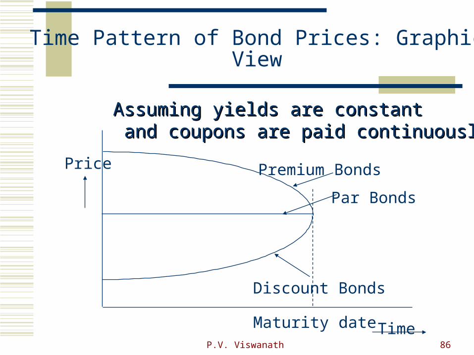
Time Pattern of Bond Prices

Bonds, like any other asset, represent an investment by the bondholder.

As such, the bondholder expects a certain total return by way of capital appreciation and coupon yield.

This implies a particular pattern of bond price movement over time.

P.V. Viswanath 86

Time Pattern of Bond Prices: Graphic View

Discount Bonds

Premium Bonds

Par Bonds

Maturity date Time

Price

Assuming yields are constantAssuming yields are constant and coupons are paid continuouslyand coupons are paid continuously

P.V. Viswanath 87

Time Pattern of Bond Prices in Practice

Coupons are paid semi-annually. Hence the bond price would increase at the required rate of return between coupon dates.

On the coupon payment date, the bond price would drop by an amount equal to the coupon payment.

To prevent changes in the quoted price in the absence of yield changes, the price quoted excludes the amount of the accrued coupon.

Example: An 8% coupon bond quoted at 96 5/32 on March 31, 2008, paying its next coupon on June 30, 2008 would actually require payment of 961.5625 + 0.5(80/2) = $981.5625