introduction to transport lecture 7 introduction to transport lecture 7: signal coordination

INTRODUCTION TO TRANSPORT

Lecture 7

Introduction to Transport

Lecture 7: Signal Coordination


Lecture 7

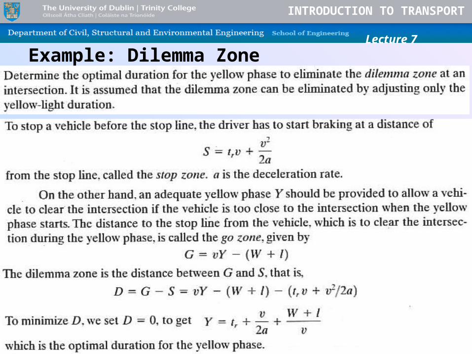
Example: Dilemma Zone


Lecture 7

Example: Dilemma Zone

A driver travelling at the speed limit of 30 mph was cited for crossing an intersection on red. He claimed that he was innocent because the duration of the amber display was improper and, consequently, a dilemma zone existed at that location. Using the following data, determine whether the driver’s claim was correct.

Amber duration = 4.5 s

Perception reaction time = 1.5 s

Comfortable deceleration = 10 ft/s2

Car length = 15 ft

Intersection width = 50 ft

(1 mile = 5280 feet)

There is a dilemma zone of 29.8 ft. Otherwise, it is unknown whether the vehicle was within the dilemma zone at the onset of amber of whether the driver was speeding cannot be proven.


Lecture 7

Example: Signal TimingRecommend an appropriate signal timing for the intersection shown in the figure. The PHF is 0.92, and moderate numbers of pedestrians are present. The intersection should operate at 0.90 of its capacity during the worst 15-minutes of the peak hour, for which volumes are shown in the figure.


Lecture 7

Solution

• The problem is designed for right hand drive. The solution is done accordingly.

STEP 1The first consideration is whether or not protected left-turn phases are needed for any approach.


Lecture 7

STEP 2All volumes should now be converted to equivalent "through car units" or tcu's.


Lecture 7

STEP 3At this point, a suitable phase plan must be developed, and the critical lane volumes for each phase must be identified.

A ring diagram showing the proposed phase plan, together with lane volumes moving in each phase is shown. The lane volumes given in the diagram are on per lane basis.The critical lane volumes are underlined by red.


Lecture 7

In Phase A, the NB and SB LT movements are given protection. Since each of these movements operates out of a separate lane, the per lane volume is equal to the total volume for each movement. The larger of 2 volumes, or 263 tcus/lane/hr, is the critical volume for this phase. In Phase B, TH and RT movements from NB and SB approaches have the green. Both of these combined movements have 2 lanes each. For the NB approach, 944/2 = 472; for the SB approach, 1,031/2 = 516. The critical volume for this phase is SB volume. In Phase C, 4 sets of movements are given the green. The EB and WB LT movements have exclusive lanes; their per lane volume is equal to the movement volume. The EB and WB TH and RT movements share 2-lane approaches. For EB approach, 702/2 = 351 tcu/lane/hr; for the WB approach, 566/2 = 283 tcu/lane/hr. The critical volume for this phase is the highest of the 4 volumes moving during the phase (WB LT movement 375 tcu/lane/hr).

The sum of critical lane volumes for this signal phases, therefore, 263 + 516 + 375 = 1155 tcu/hr


Lecture 7

STEP 4The desired cycle length can now be computed,

The min. cycle time, 65.7 sec.Assuming that a pre-timed signal is in use, use 70s as the cycle length, as timing dials are commonly available in 5-second increments.

)/(16151

3

)/3600)(/(1

cvPHFVN

hcvPHFVNt

Ccc

Ldes


Lecture 7

STEP 5The allocation of available effective green time in proportion to the critical lane volumes for each phase. The effective green time is the cycle time minus the lost time in the cycle, or 70 (3)(3)= 61 seconds.


Lecture 7

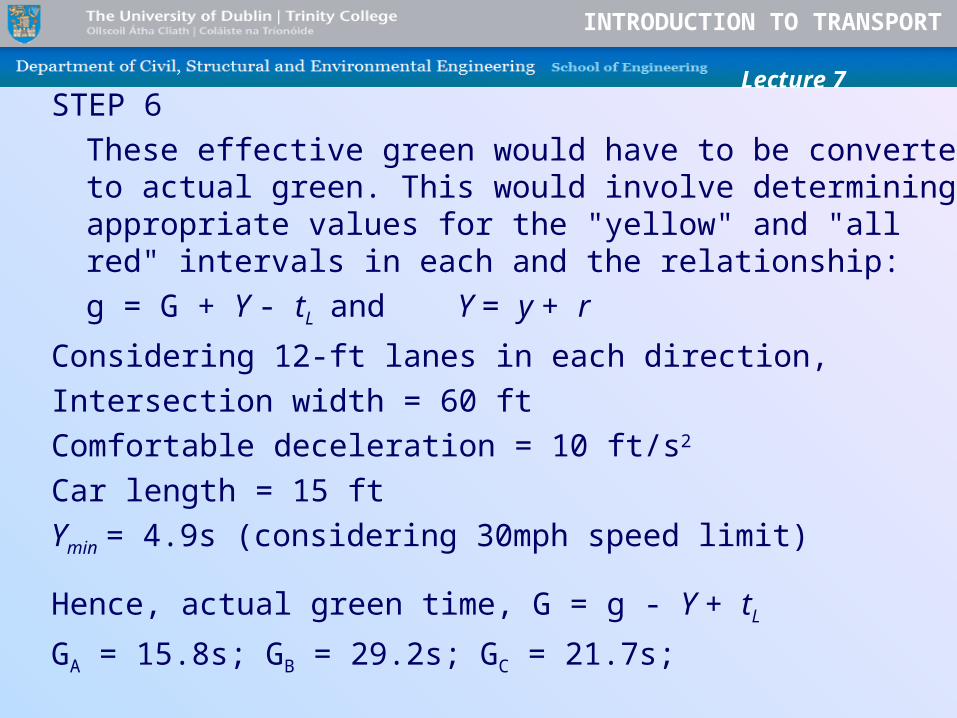
STEP 6These effective green would have to be converted to actual green. This would involve determining appropriate values for the "yellow" and "all red" intervals in each and the relationship:

g = G + Y - tL and Y = y + r

Considering 12-ft lanes in each direction, Intersection width = 60 ftComfortable deceleration = 10 ft/s2

Car length = 15 ftYmin = 4.9s (considering 30mph speed limit)

Hence, actual green time, G = g - Y + tL

GA = 15.8s; GB = 29.2s; GC = 21.7s;


Lecture 7

STEP 7Pedestrian crossing times should also be checked to insure that these green times allow for safe crossing, if a deficiency for pedestrians is noted, the cycle would normally be increased, and the green time reallocated in the same proportion as this solution.

Min. pedestrian crossing time, =5.5(moderate) + 60/4 = 20.5sPhase A, 15.8+4.9 = 20.7s>20.5s

Hence, safety requirements are met.


Lecture 7

Example: Pedestrian Requirement

Does the signal adequately accommodate pedestrians?


Lecture 7

1. Calculate Min. green time required for pedestrians.

2. Check whether available green time is enough.3. If not increase the required phase to nearest

multiple of 5 or 0.4. The ratio of the green phases at two approaches

should be kept the same.

45

20 15A

G Y


Lecture 7

Area Traffic Control

• Where signals are closely spaced, coordination is necessary to avoid queue spillback, to minimize stops and delays.

• Green Wave: When a series of traffic lights (usually three or more) are coordinated to ensure continuous green phase and traffic flow without stops over several intersections in one main direction.

• Common practise is to coordinate signals less than 1000ft apart.

• Most coordination schemes require same cycle length for all signals.


Lecture 7

Time space diagram


Lecture 7

Offset


Lecture 7

Signal Progression in 1-way street• Determining ideal offset

Assuming no vehicles are queued at the signals, the ideal offsets can be determined assuming a desired platoon speed of 60 fps.


Lecture 7

Signal Progression in 1-way street• Time space diagram

3. The MSG of the next downstream signal should be located next, relative to t = 0. With this point located (Point 2), fill in the periods of green, yellow, and red for this signal.

4. Repeat the procedure for all other intersections, working 1 at a time.

1. The vertical should be scaled so as to accommo date the dimensions of the arterial, and the hori zontal so as to accommodate at least three to four cycle lengths.

2. The beginning intersection should be scaled first, usually with MSG initiation at t = 0, followed by green and red phase (yellow may be shown for precision). See Point 1.


Lecture 7

Signal Progression in 1-way street• Effects of vehicles queued

The lost time is counted only at the first downstream intersection, at most: If the vehicle(s) from the preceding intersection were themselves stationary, their start-up causes a shift that automatically takes care of the start-up at later intersections.


Lecture 7

The time-space diagram for the example, given queues of 2 vehicles per lane in all links. The arriving vehicle platoon has a smooth flow, and the lead vehicle has 60 fps travel speed. The visual image of the "green wave" or progression speed is much faster. The "green wave“ is travelling at varying speeds as it moves down the arterial.


Lecture 7

Expected questions• TheoryJunction, junction designTraffic signs (classification and details)Types of traffic signal control (description and comparison)Discharge headway, different types of lost timeDifferent types of capacity calculationDelay

• Numerical ProblemsTraffic signal designArea traffic controlAll examples given in lectures

introduction to transport lecture 7 introduction to transport lecture 7: signal coordination

Documents