introduction to theoretical elementary particle physics ...stefanw/download/script_qft2.pdf ·...
TRANSCRIPT

Introduction to Theoretical Elementary Particle
Physics:
Relativistic Quantum Field Theory
Part II
Stefan Weinzierl
August 1, 2018
1

Contents
1 Overview 4
1.1 Literature . . . . . . . . . . . . . . . . . . . . . . . . . . . . . . . . . . . . . . 4
2 Review of quantum field theory 4
2.1 Path integral formalism . . . . . . . . . . . . . . . . . . . . . . . . . . . . . . . 4
2.2 Cross sections and decay rates . . . . . . . . . . . . . . . . . . . . . . . . . . . 5
2.3 Gauge theory . . . . . . . . . . . . . . . . . . . . . . . . . . . . . . . . . . . . 6
2.4 Fermions in the fundamental representation of the gauge group . . . . . . . . . . 7
2.5 Feynman rules for QED and QCD . . . . . . . . . . . . . . . . . . . . . . . . . 8
3 The Standard Model 12
3.1 Spontaneous symmetry breaking . . . . . . . . . . . . . . . . . . . . . . . . . . 12
3.2 The Higgs mechanism . . . . . . . . . . . . . . . . . . . . . . . . . . . . . . . 13
3.3 Yukawa couplings . . . . . . . . . . . . . . . . . . . . . . . . . . . . . . . . . . 16
3.4 Feynman rules in the electroweak sector . . . . . . . . . . . . . . . . . . . . . . 17
3.5 Flavour mixing . . . . . . . . . . . . . . . . . . . . . . . . . . . . . . . . . . . 20
3.6 Summary of the Standard Model . . . . . . . . . . . . . . . . . . . . . . . . . . 24
4 Loop integrals 26
4.1 Regularisation . . . . . . . . . . . . . . . . . . . . . . . . . . . . . . . . . . . . 27
4.2 Loop integration in D dimensions . . . . . . . . . . . . . . . . . . . . . . . . . 27
4.2.1 Feynman and Schwinger parameterisation . . . . . . . . . . . . . . . . . 28
4.2.2 Shift of the integration variable . . . . . . . . . . . . . . . . . . . . . . 29
4.2.3 Wick rotation . . . . . . . . . . . . . . . . . . . . . . . . . . . . . . . . 30
4.2.4 Generalised spherical coordinates . . . . . . . . . . . . . . . . . . . . . 32
4.2.5 Euler’s gamma and beta functions . . . . . . . . . . . . . . . . . . . . . 33
4.2.6 Result for the momentum integration . . . . . . . . . . . . . . . . . . . 34
4.3 Performing the Feynman integrals . . . . . . . . . . . . . . . . . . . . . . . . . 36
4.3.1 The one-loop tadpole . . . . . . . . . . . . . . . . . . . . . . . . . . . . 36
4.3.2 The one-loop two-point function . . . . . . . . . . . . . . . . . . . . . . 37
4.3.3 More general methods . . . . . . . . . . . . . . . . . . . . . . . . . . . 39
4.4 Tensor integrals and Passarino-Veltman reduction . . . . . . . . . . . . . . . . . 39
5 Renormalisation 42
5.1 Renormalisation in practice . . . . . . . . . . . . . . . . . . . . . . . . . . . . . 43
5.1.1 Renormalisation of the coupling constant . . . . . . . . . . . . . . . . . 44
5.1.2 Mass renormalisation . . . . . . . . . . . . . . . . . . . . . . . . . . . . 46
5.2 Renormalisation to all orders . . . . . . . . . . . . . . . . . . . . . . . . . . . . 51
5.2.1 Power counting . . . . . . . . . . . . . . . . . . . . . . . . . . . . . . . 51
5.2.2 Hopf algebras . . . . . . . . . . . . . . . . . . . . . . . . . . . . . . . . 52
5.2.3 Renormalisation revisited . . . . . . . . . . . . . . . . . . . . . . . . . 55
2

6 Mathematical structures of loop integrals 58
6.1 General tensor integrals . . . . . . . . . . . . . . . . . . . . . . . . . . . . . . . 59
6.2 Expansion of transcendental functions . . . . . . . . . . . . . . . . . . . . . . . 60
6.3 Nested Sums . . . . . . . . . . . . . . . . . . . . . . . . . . . . . . . . . . . . 61
6.4 Expansion of hypergeometric functions . . . . . . . . . . . . . . . . . . . . . . 66
6.5 The integral representation of multiple polylogarithms . . . . . . . . . . . . . . 68
6.6 The antipode and integration-by-parts . . . . . . . . . . . . . . . . . . . . . . . 71
6.7 Numerical evaluation of multiple polylogarithms . . . . . . . . . . . . . . . . . 73
6.8 Mellin-Barnes integrals . . . . . . . . . . . . . . . . . . . . . . . . . . . . . . . 74
7 From differential geometry to Yang-Mills theory 75
7.1 Manifolds . . . . . . . . . . . . . . . . . . . . . . . . . . . . . . . . . . . . . . 75
7.2 Differential forms . . . . . . . . . . . . . . . . . . . . . . . . . . . . . . . . . . 76
7.3 Riemannian geometry . . . . . . . . . . . . . . . . . . . . . . . . . . . . . . . . 77
7.4 Hodge theory . . . . . . . . . . . . . . . . . . . . . . . . . . . . . . . . . . . . 81
7.5 The covariant derivative . . . . . . . . . . . . . . . . . . . . . . . . . . . . . . . 82
7.6 Fibre bundles . . . . . . . . . . . . . . . . . . . . . . . . . . . . . . . . . . . . 84
7.7 Connections on fibre bundles . . . . . . . . . . . . . . . . . . . . . . . . . . . . 86
7.8 Instantons . . . . . . . . . . . . . . . . . . . . . . . . . . . . . . . . . . . . . . 91
7.9 Chern classes and Chern characters . . . . . . . . . . . . . . . . . . . . . . . . . 94
8 Supersymmetry 96
8.1 Groups and symmetries of space-time . . . . . . . . . . . . . . . . . . . . . . . 96
8.1.1 The Poincaré group . . . . . . . . . . . . . . . . . . . . . . . . . . . . . 96
8.1.2 The homogeneous Lorentz group . . . . . . . . . . . . . . . . . . . . . 96
8.2 Mixing internal symmetries with space-time symmetries . . . . . . . . . . . . . 97
8.3 Grassmann algebra . . . . . . . . . . . . . . . . . . . . . . . . . . . . . . . . . 97
8.4 Sign conventions . . . . . . . . . . . . . . . . . . . . . . . . . . . . . . . . . . 98
8.5 Superspace . . . . . . . . . . . . . . . . . . . . . . . . . . . . . . . . . . . . . 99
8.6 Supersymmetric fields . . . . . . . . . . . . . . . . . . . . . . . . . . . . . . . 100
8.6.1 Chiral super-fields . . . . . . . . . . . . . . . . . . . . . . . . . . . . . 100
8.6.2 Vector super-fields . . . . . . . . . . . . . . . . . . . . . . . . . . . . . 101
8.7 Transformation of the fields . . . . . . . . . . . . . . . . . . . . . . . . . . . . . 102
8.8 Lagrange density for supersymmetric QCD . . . . . . . . . . . . . . . . . . . . 103
8.9 Supersymmetry breaking . . . . . . . . . . . . . . . . . . . . . . . . . . . . . . 105
8.10 Supersymmetric relations . . . . . . . . . . . . . . . . . . . . . . . . . . . . . . 106
8.11 Spontaneous breaking of supersymmetry . . . . . . . . . . . . . . . . . . . . . . 108
8.11.1 The mechanism of O’Raifeartaigh . . . . . . . . . . . . . . . . . . . . . 108
8.11.2 The mechanism of Fayet and Iliopoulos . . . . . . . . . . . . . . . . . . 108
8.12 The minimal supersymmetric standard model . . . . . . . . . . . . . . . . . . . 108
3

1 Overview
1.1 Literature
There is no shortage of text books on quantum field theory. I will list a few of them here:
- M. Peskin und D. Schroeder, An Introduction to Quantum Field Theory, Perseus Books, 1995.
- M. Schwartz, Quantum Field Theory and the Standard Model, Cambridge University Press,
2014.
- M. Srednicki, Quantum Field Theory, Cambridge University Press, 2007.
Lecture notes (on more specialised topics):
- S. Weinzierl, The art of computing loop integrals, arXiv:hep-ph/0604068
- S. Weinzierl, Tales of 1001 Gluons, arXiv:1610.05318
2 Review of quantum field theory
We start with a review of the basics of quantum field theory. We will assume that these concepts
have been covered in a first course on quantum field theory, therefore the exposition in this
section will be brief.
2.1 Path integral formalism
The generating functional is given by
Z[J(x)] = N
∫Dφ(x) exp
[
i
∫d4x L(φ)+ J(x)φ(x)
]
.
Functional derivatives are defined by
δ
δJ(y)Z [J(x)] = lim
ε→0
Z [J(x)+ εδ(x− y)]−Z [J(x)]
ε.
The n-point Green functions are obtained as functional derivatives of Z[J]:
⟨Ω∣∣T φ(x1)...φ(xn)
∣∣Ω⟩
= Gn(x1, ...,xn) =(−i)n
Z[0]
δnZ[J(x)]
δJ(x1)...δJ(xn)
∣∣∣∣J=0
The functional Z[J] generates all Green functions:
Z[J] = Z[0]∑n
in
n!
∫d4x1...d
4xn
⟨Ω∣∣T φ(x1)...φ(xn)
∣∣Ω⟩
J(x1)...J(xn)
4

For the computation of scattering amplitudes we would like to have as boundary condition not
the vacuum but an n particle state. If we assume that interactions are only relevant within a finite
volume, we can take this n particle state as the superposition of n non-interacting one-particle
states. We call such a state an asymptotic state. If we consider a scalar field theory, the asymptotic
field satisfies the Klein-Gordon equation
(+m2
)φasymp(x) = 0.
Consider now
Zasymp [J] =∫
limφ=φasymp
Dφ exp
[
i
∫d4x L(φ)+ J(x)φ(x)
]
.
Then
Zasymp [0] =
∑in
n!
∫d4x1...d
4xnφasymp(x1)...φasymp(xn)(x1
+m2)...(xn
+m2)
Gn(x1, ...,xn).
Define now the Fourier transform of the Green functions by
Gn(x1, ...,xn) =∫
d4p1
(2π)4...
d4pn
(2π)4e−i∑ p jx j (2π)4 δ4 (p1 + ...+ pn) Gn(p1, ..., pn)
and the truncated (amputated) Green function in momentum space by
Gntrunc(p1, ..., pn) =
(i
p21 −m2
)−1
...
(i
p2n −m2
)−1
Gn(p1, ..., pn).
2.2 Cross sections and decay rates
To calculate the cross section at an collider with no initial-state hadrons (e.g. an electron-positron
collider):
σ =1
2K(Q2)
1
nspin(A)nspin(B)
∫dφ(pA + pB; p1, ..., pn) |A (pA pB → p1 p2...)|2
where 2K(Q2) is the flux factor and we have 2K(Q2) = 2Q2 for massless incoming particles.
The scattering amplitudes is given by
A (pA pB → p1 p2...) = Gntrunc,connected (pA pB → p1 p2...) .
For a decay rate we have
Γ =1
2mA
1
nspin(A)
∫dφ(pA; p1, ..., pn) |A (pA → p1 p2...)|2 .
5

The phase-space measure is given by
dφ(Q; p1, p2, ..., pn) =1
∏ j n j!
(
∏f
d3p f
(2π)32E~p f
)
(2π)4δ4(Q−∑ p f ),
if the final state contains n j identical particles of type j. If the colliding particles are not elemen-
tary (like protons or antiprotons), we have to include the probability of finding the elementary
particle A inside the proton or antiproton. If the proton has momentum pp one usually specifies
the probability of finding a parton with momentum fraction x by the parton distirbution function
f (x).
The parton has then the momentum
pA = xpp.
For the cross section we have to integrate over all possible momentum fractions and the formula
for a hadron-hadron collider becomes
σ =∫
dx1 f (x1)∫
dx2 f (x2)1
2K(s)
1
nspin(A)nspin(B)
1
ncolour(A)ncolour(B)∫dφ(pA + pB; p1, ..., pn) |A (pA pB → p1p2...)|2 .
ncolour(A) and ncolour(B) are the number of colour degrees of the initial state particles.
2.3 Gauge theory
An important example of a quantum field theory is given by gauge theories. Gauge theories (also
called Yang-Mills theories) are characterised by the fact that at each point in space-time we have
an internal symmetry group G. Let us now briefly review Yang-Mills theory.
Let G be a Lie group, g its Lie algebra and T a the generators of the Lie algebra where the
index a takes values from 1 to dimG. We use the conventions
[
T a,T b]
= i f abcT c, Tr(
T aT b)
=1
2δab.
The Lie group is called abelian, if all structure constants f abc vanish, otherwise it is called non-
abelian. In particle physics we encounter abelian and non-abelian gauge groups. An example for
the abelian case is given by quantum electrodynamics (QED), corresponding to the abelian gauge
group U(1). An example for the non-abelian case is given by quantum chromodynamics (QCD),
corresponding to the non-abelian gauge group SU(3). The extension towards non-abelian gauge
groups was first suggested by Yang and Mills in 1954, hence the name “Yang-Mills theory” as
a synonym for “gauge theory”. We may view the abelian case as a special case of the general
non-abelian case.
6

The field strength tensor is given by
Faµν = ∂µAa
ν −∂νAaµ +g f abcAb
µAcν,
where a is an index running over all generatros of the Lie algebra. For a SU(N) gauge group the
index a runs from 1 to N2 −1. The Lagrange density reads:
L = −1
4Fa
µνFaµν.
The Lagrange density is invariant under the local transformations
T aAaµ(x) → U(x)
(
T aAaµ(x)+
i
g∂µ
)
U†(x)
with
U(x) = exp(−iT aθa(x)) .
The action is given by the integral over the Lagrange density:
S =
∫d4x L .
The quantity
LGF = − 1
2ξ
(∂µAa
µ
)(∂νAa
ν)
is called the gauge-fixing term, the quantity
LFP = −ca∂µDabµ cb
the Faddeev-Popov term.
2.4 Fermions in the fundamental representation of the gauge group
We recall that the Lagrange density for a free fermion (e.g. no interactions) is given by
LF = ψ(iγµ∂µ −m)ψ.
We are now looking for a Lagrange density for the fermionic sector, which remains invariant
under gauge transformations. Under a gauge transformation a fermion field ψi(x) transforms as
ψi(x)→Ui j(x)ψ j(x), Ui j(x) = exp(−iT aθa(x)) ,
ψi(x)→ ψ j(x)U†ji(x).
7

θa(x) depends on the space-time coordinates x. For an infinitessimal gauge transformation we
have
ψi(x) → (1− iT aθa(x))ψ j(x).
We immediately see that a fermion mass term
−mψ(x)ψ(x)
is invariant under gauge transformations. (Note however that in the standard model the fermion
masses are generated through the Yukawa couplings to the Higgs field.) But the term involving
derivatives is not gauge invariant:
iψ(x)γµ∂µψ(x) → iψ(x)U†(x)γµ∂µ (U(x)ψ(x))
= iψ(x)γµ∂µψ(x)+ iψ(x)γµ(
U†(x)∂µU(x))
ψ(x)︸ ︷︷ ︸
extra
.
The solution comes in the form of the covariant derivative
Dµ = ∂µ − igT aAaµ(x),
where the gauge field transforms as
T aAaµ(x) → U(x)
(
T aAaµ(x)+
i
g∂µ
)
U†(x).
Then the combination
iψ(x)γµDµψ(x) = iψ(x)γµ(∂µ − igT aAa
µ(x))
ψ(x)
→ iψ(x)U†(x)γµ
[
∂µ − igU(x)
(
T aAaµ(x)+
i
g∂µ
)
U†(x)
]
U(x)ψ(x)
= iψ(x)γµ∂µψ(x)+ iψ(x)γµ(
U†(x)∂µU(x))
ψ(x)
+gψ(x)γµT aAaµ(x)ψ(x)+ iψ(x)γµ
[(
∂µU†(x))
U(x)]
ψ(x)
is invariant.
This gives us the Lagrange density for the fermion sector:
Lfermions = ∑fermions
ψ(x)(iγµDµ −m f
)ψ(x).
2.5 Feynman rules for QED and QCD
From the Lagrange density we may derive the Feynman rules. We summarise here the Feynman
rules for QED and QCD.
8

Propagators:
The propagators for the gauge bosons are in the Feynman gauge (ξ = 1).
gauge bosons gluon Aaµ
−igµν
k2 δab
photon Aµ−igµν
k2
fermions quarks ψi ip/+m
p2−m2 δi j
leptons ψ ip/+m
p2−m2
ghosts ca ik2 δab
Vertices:
Quark-gluon-vertex:
igγµT ai j
3-gluon-vertex:
k1,µ,a
k2,ν,bk3,λ,c
g f abc[(k2 − k3)µgνλ +(k3 − k1)νgλµ +(k1 − k2)λgµν
]
4-gluon-vertex:
µ,a
ν,bλ,c
ρ,d
9

−ig2[
f abe f ecd(gµλgνρ−gµρgνλ
)+ f ace f ebd
(gµνgλρ −gµρgλν
)+ f ade f ebc
(gµνgλρ −gµλgνρ
)]
Gluon-ghost-vertex:
µ,b
q,c
k,a
−g f abckµ
Fermion-photon-vertex:
ieQγµ
Additional rules:
An integration
∫d4k
(2π)4
for each loop.
A factor (−1) for each closed fermion loop.
Symmetry factor: Multiply the diagram by a factor 1/S, where S is the order of the permuta-
tion group of the internal lines and vertices leaving the diagram unchanged when the external
lines are fixed.
External particles:
Outgoing fermion: u(p)Outgoing antifermion: v(p)
Incoming fermion: u(p)Incoming antifermion: v(p)
Gauge boson: εµ(k)
10

Polarisation sums:
∑λ
u(p,λ)u(p,λ) = p/+m,
∑λ
v(p,λ)v(p,λ) = p/−m,
∑λ
ε∗µ(k,λ)εν(k,λ) = −gµν +kµnν +nµkν
kn−n2 kµkν
(kn)2.
Here nµ is an arbitrary four vector. The dependence on nµ cancels in gauge-invariant quantities.
Using Weyl spinors, a convenient choice of polarisation vectors for the gauge bosons is given by
ε+µ (k,q) =〈q−|γµ|k−〉√
2〈qk〉,
ε−µ (k,q) =〈q+ |γµ|k+〉√
2 [kq],
where qµ is an arbitrary light-like reference momentum. The dependence on qµ cancels in gauge-
invariant quantities.
11

3 The Standard Model
3.1 Spontaneous symmetry breaking
The concept of gauge theories allowed us to describe successfully quantum electrodynamics and
quantum chromodynamcis, the quantum theories of the electromagnetic and the strong force.
Both theories are characterised by the fact, that the particles which mediate the forces (photons
and gluons) are massless particles. This is required by gauge invariance. In fact, a naive mass
term for the gauge bosons in the Lagrangian
Lmass = m2AaµAa µ
is not invariant under gauge invariance
T aAaµ(x) → U(x)
(
T aAaµ(x)+
i
g∂µ
)
U†(x).
On the other hand it is an experimental fact, that the W -bosons and the Z-boson have non-zero
masses. As we do not want to abandon the concept of gauge theories, we face the problem on how
to incoporate massive gauge bosons into gauge theories. The solution is provided by the concept
of spontaneously broken gauge theories, also known under the name “Higgs mechanism”. To
start the discussion let us consider a simple physical system with a complex coordinate φ and a
potential
V (φ) = m2 |φ|2 + 1
4λ(
|φ|2)2
.
The potential has a harmonic term m2 |φ|2 and an anharmonic term 14λ(
|φ|2)2
. For m2 > 0 and
λ > 0 the potential has an absolut minimum at φ = 0. In classical mechanics the ground state
would therefore be φ = 0. This is nothing new.
Imagine now that the potential is given by
V (φ) = −µ2 |φ|2 + 1
4λ(
|φ|2)2
,
with
µ2 > 0, λ > 0.
Then the potential has the shape of a mexican hat, and φ = 0 corresponds to a local maxima. The
potential has a minima for
|φ|2 =2µ2
λ.
12

The minimas are described by a circle in the complex plane. The ground state of the physical
system will be one point of this circle, with no preference for any particular point. Without loss
of generality we can choose this point to lie along the positive real axis. Therefore we face the
situation, that the potential has a rotational symmetry around the point φ = 0, while the ground
state has not. This is the concept of a spontaneously broken symmetry. In general one speaks
about a spontaneously broken symmetry, if the Lagrangian of a theory has a certain symmetry,
which is not preserved in the ground state of the theory.
3.2 The Higgs mechanism
The standard model is based on the gauge group
SU(3)×SU(2)×U(1),
where SU(3) is the gauge group of the strong interactions, SU(2) the gauge group associated
to the weak isospin and U(1) the gauge group associated to the hypercharge. This group is not
identical to the gauge group of quantum electrodynamics. To avoid confusions, one often writes
UY (1) for the group related to the hypercharge and Uel−magn(1) for the gauge group of QED.
In the standard model, the electroweak sector SU(2)×UY(1) is spontaneously broken down to
Uel−magn(1). We now study the spontaneously symmetry breakdown in detail.
Within the standard model one assumes an additional complex scalar field, transforming as the
fundamental representation of SU(2) and having hypercharge Y = 1. In the weak isospin space
we can write the field as a two-vector with complex entries. It will be conveninet to use the
following parametrisation:
φ(x) =
(
φ+(x)1√2(v+H(x)+ iχ(x))
)
.
φ+(x) is a complex field (two real components), H(x) and χ(x) are real fields. The quantity v is
a real constant. We will later see that it corresponds to the vacuum expectation value of the field
φ(x). The three components φ(x) and χ(x) are absorbed as the longitudinal modes of W±µ and Zµ.
H(x) is the Higgs field.
The Lagrange density of the Higgs sector
LHiggs =(Dµφ
)†(Dµφ)−V (φ)+LYukawa.
The covariant derivative is given by
Dµ = ∂µ − igIaW aµ − ig′
Y
2Bµ,
where Ia = 12σa (σa are the Pauli matrices) and we have Y = 1 for the Higgs doublet. (Note that
our g′ =−g1 (Hollik).)
13

The Higgs potential is given by
V (φ) = −µ2φ†φ+1
4λ(
φ†φ)2
.
For µ2 > 0 (and λ > 0) we have spontaneous symmetry breaking. In that case the potential has a
minimum for
φ†φ =2µ2
λ=
v2
2.
We have
v = 2
√
µ2
λ.
We write
φ(x) =
(
φ+(x)1√2(v+H(x)+ iχ(x))
)
,
φ†(x) =
(
φ−(x),1√2(v+H(x)− iχ(x))
)
.
We introduced this parametrisation already previously. We now see that this parametrisation
corresponds to an expansion around the minimum of the potential V (φ). Indeed, we have for
φ+(x) = 0 and H(x) = χ(x) = 0:
φ(x) =v√2
(0
1
)
,
giving us one point in the minimum of the potential. All points in the minimum of the potential
are parametrised with two parameters α and β through
φ(x) =v√2
(eiα sinβeiα cosβ
)
.
We have to pick a point in the minimum of the potential, any choice of point is as good as
any other choice. The choive made above is the conventional choice. With the parametrisation
around the minimum as above let us now consider the terms bilinear in the fields W aµ and Bµ
coming from (Dµφ)†(Dµφ). We find
(Dµφ
)† (Dµφ
)∣∣∣W a
µ ,Bµ−bilinear=
1
8g2v2
(W 1
µ W 1µ +W 2
µ W 2µ
)
+1
8v2(Bµ,W
3µ
)(
g′2 −gg′
−gg′ g2
)(Bµ
W 3µ
)
.
14

We define
W±µ =
1√2
(W 1
µ ∓ iW 2µ
)
and(
Aµ
Zµ
)
=
(cosθW sinθW
−sinθW cosθW
)(Bµ
W 3µ
)
.
The angle θW is given by
cosθW =g
√
g2 +g′2, sinθW =
g′√
g2 +g′2.
θW is called the Weinberg angle. We then obtain
(Dµφ
)† (Dµφ
)∣∣∣W a
µ ,Bµ−bilinear=
1
2
(vg
2
)2 (W+
µ∗W+
µ +W−µ
∗W−
µ
)
+1
2
(v
2
√
g2 +g′2)2(Aµ,Zµ
)(
0 0
0 1
)(Aµ
Zµ
)
.
We therefore have
mW =v
2g, mZ =
v
2
√
g2 +g′2.
It is not too difficult to show that the Higgs mass is given by
mH =
√
λ
2v.
In order to see this, we look at all terms bilinear in H from
−V (φ)|H−bilinear = µ2φ†φ− 1
4λ(
φ†φ)2∣∣∣∣H−bilinear
= −1
2
(
−µ2 +3
4λv2
)
H2 = −1
2
(λv2
2
)
H2.
The gauge couplings g and g′ are related to the elementary electric charge by
e =gg′
√
g2 +g′2,
or
g =e
sinθW, g′ =
e
cosθW.
15

3.3 Yukawa couplings
The Higgs sector generates also the fermion masses through Yukawa couplings. We discuss this
mechanism first in a simplified model without flavour mixing. The full standard model including
flavour mixing is discussed in the next section 3.5.
Spin 1/2 particles are described by four-component spinors ψ(x). With the chiral projectors
P± =1
2(1± γ5)
we define left- and right-handed spinors:
ψ±(x) = P±ψ(x).
The fermions in the standard model can be grouped into three families:
u
d
νe
e
,
c
s
νµ
µ
,
t
b
ντ
τ
.
The families differ only by the masses of their members.
Let us now discuss the quantum numbers of the fermions in the electro-weak sector:
The left-handed components (uL,dL) and (νL,eL) transform as the fundamental representation
under the SU(2) group. The right-handed components uR, dR, νR and eR transform as a singlet
under the SU(2) group.
In detail one has:
I3 Y Q
uL12
13
23
dL −12
13
−13
νL12
−1 0
eL −12
−1 −1
I3 Y Q
uR 0 43
23
dR 0 −23
−13
νR 0 0 0
eR 0 −2 −1
The electric charge is given by the Gell-Mann-Nishijima formula:
Q = I3 +Y
2
Remark: The table contains a right-handed neutrino, which does not interact with any other par-
ticle.
16

The Yukawa couplings are given by
LYukawa =
∑families
−λd
(uL, dL
)φdR −λu
(uL, dL
)φCuR −λe (νL, eL)φeR −λν (νL, eL)φCνR + h.c.
,
where the charge-conjugate Higgs field is given by
φC = 2iI2φ∗ = iσ2φ∗ =(
0 1
−1 0
)(
φ−(x)1√2(v+H(x)− iχ(x))
)
=
(1√2(v+H(x)− iχ(x))
−φ−(x)
)
.
Example:
−λd
(uL, dL
)φdR + h.c. = −λd
(uL, dL
)
(
φ+(x)1√2(v+H(x)+ iχ(x))
)
dR + h.c.
= −vλd√2
(uL, dL
)(
0
1
)
dR + interaction terms+ h.c.
= −vλd√2
dLdR + interaction terms+ h.c.
Therefore the Yukawa couplings generate the masses of the fermions. From the above example
we obtain
md =1√2
vλd .
The case of the up-type masses is similar. We have for example
−λu
(uL, dL
)φCuR + h.c. = −λu
(uL, dL
)
(1√2(v+H(x)− iχ(x))
−φ−(x)
)
uR + h.c.
= −vλu√2
(uL, dL
)(
1
0
)
uR + interaction terms+ h.c.
= −vλu√2
uLuR + interaction terms+ h.c.,
giving us
mu =1√2
vλu.
3.4 Feynman rules in the electroweak sector
In this paragraph we present the most important Feynman rules in the electroweak sector. A
complete list of Feynman rules can be found in many textbooks. We present the Feynman rules
17

for the fields Aµ, Zµ and W±µ . The original fields are related to the new fields by
(Bµ
W 3µ
)
=
(cosθW −sinθW
sinθW cosθW
)(Aµ
Zµ
)
,
(W 1
µ
W 2µ
)
=1√2
(1 1
i −i
)(W+
µ
W−µ
)
.
As with any gauge theory, we also have to fix the gauge for the electroweak sector. A useful
gauge fixing condition is given in the electroweak sector by the ’t Hooft gauge (also called Rξ-
gauge):
LGF =
− 1
ξW(∂µW+
µ − imW ξW φ+)(∂µW−µ + imW ξW φ−)− 1
2ξZ(∂µZµ −mZξZχ)2
︸ ︷︷ ︸
SU(2)
− 1
2ξγ(∂µAµ)
2
︸ ︷︷ ︸
U(1)
ξ = 0 corresponds to Landau gauge, ξ = 1 to the Feynman gauge. φ+, φ− and χ are called the
would-be Goldstone fields. For the propagators we have to look at all terms in the Lagrangian,
which contain exactly two fields. LHigss will contain terms, which involve one electroweak gauge
boson (Zµ, W±µ ) and one pseudo-Goldstone field (χ, φ±). These terms lead to a mixing between
electroweak gauge bosons and pseudo-Goldstone fields, resulting in a propagator matrix. The ’t
Hooft Rξ-gauge eliminates these mixing terms.
The propagators for the W - and Z-bosons are given in ’t Hoofts Rξ=1-gauge by
gauge bosons photon Aµ−igµν
k2
W-boson W±µ
−igµν
k2−m2W
Z-boson Zµ−igµν
k2−m2Z
Higgs sector Higgs H i
k2−m2H
Let us now look at the interaction vertices of the electroweak gauge bosons with fermions. We
have for the covarariant derivative
Dµ = ∂µ − igIaW aµ − ig′
Y
2Bµ
= ∂µ − iQeAµ −ie
2sinθW cosθW
(2I3 −2Qsin2 θW
)Zµ
− ie√2sinθW
(I1+ iI2
)W+
µ − ie√2sinθW
(I1 − iI2
)W+
µ .
18

Note that
I1 + iI2 =
(0 1
0 0
)
, I1− iI2 =
(0 0
1 0
)
.
Thus we obtain
ψiγµDµψ∣∣trilinear
= ψγµψ
[
QeAµ +e
2sinθW cosθW
(2I3−2Qsin2 θW
)Zµ
+e√
2sinθW
(I1 + iI2
)W+
µ +e√
2sinθW
(I1− iI2
)W+
µ
]
.
Thus we see that the photon-fermion-antifermion vertex is iQeγµ, as already known from QED.
The Z-fermion-antifermion vertex is given by
ie
2sinθW cosθW
γµ
(v f −a f γ5
),
where
v f = I3 −2Qsin2 θW , a f = I3,
and I3 equals 1/2 for up-type fermions and −1/2 for down-type fermions. The u jW+dk-vertex
is given by
ie
2√
2sinθw
γµ (1− γ5)Vjk,
the dkW−u j-vertex is given by
ie
2√
2sinθw
γµ (1− γ5)V ∗jk.
In a model without flavour mixing we have Vjk = δ jk, in the next paragraph we will study flavour
mixing in the Standard model and Vjk will be the appropriate matrix element of the quark mixing
matrix or the neutrino mixing matrix.
Let us also look at the fermion-antifermion-Higgs vertex. The vertex comes from the Yukawa
part of the Lagrange density. As Feynman rules one finds
−iλ f√
2,
where λ f is the Yukawa coupling of fermion f . Since
m f =1√2
vλ f and v =2mW
esinθW
we may equally write for the fermion-antifermion-Higgs vertex
− ie
2sinθw
m f
mW.
19

3.5 Flavour mixing
We now come to the final ingredient of the standard model: flavour mixing. Let us consider the
electroweak sector, in particular the coupling of quarks to the electroweak gauge bosons. Recall
the Lagrange density for the quark sector:
Lfermions = ∑families
(uL, d
′L
)iγµDµ
(uL
d′L
)
+ uRiγµDµuR + d′RiγµDµd′
R
For reasons, which will become clear later, we put a prime on all d-type quark fields. The
Lagrange density is obtained by replacing the ordinary derivative ∂µ with the covariant derivative
Dµ = ∂µ − igIaW aµ − ig′
Y
2Bµ.
This is required by gauge invariance. This Lagrange density does not allow for mixing between
the various quark flavours.
On the other hand the Yukawa couplings are given by
LYukawa = ∑families
−λd
(uL, dL
)φdR −λu
(uL, dL
)φCuR + h.c.
where the charge-conjugate Higgs field is given by
φC = iσ2φ∗ = 2iI2φ∗.
Note that now the prime is missing on the d-type quark fields. We have seen that the Yukawa
terms lead to mass terms for the fermions:
−λd
(uL, dL
)φdR −λu
(uL, dL
)φCuR + h.c. =
−vλd√2
dLdR −vλu√
2uLuR + h.c.+ interaction terms
However, the Yukawa couplings are not constrained by any gauge symmetry and we could allow
for flavour mixing in the Yukawa terms. In fact, nature has chosen this possibility. We therefore
consider a general mass term of the form
Lmass = ∑families
d′′LMdd′′
R + u′′LMuu′′R + h.c.
where Md and Mu are (arbitrary) complex 3× 3 matrices in family space. A matrix M can be
diagonalised by a biunitary transformation
V−1MW = M,
where M is a diagonal matrix.
Proof: Using the polar decomposition, M can be written as
M = HU,
20

where H is hermitian and U is a unitary matrix. H can be diagonalised by a unitary matrix V :
V−1HV = M,
therefore W =U−1V .
The gauge part of the Lagrange density
Lfermions = ∑families
(uL, d
′L
)iγµDµ
(uL
d′L
)
+ uRiγµDµuR + d′RiγµDµd′
R
is invariant under the rotations with respect to the family index:(
uL
d′L
)
→ SL
(uL
d′L
)
uR → SR,uuR
dR → SR,ddR
Using this freedom we have with
Mu =VuMuW−1u , Md =VdMdW−1
d ,
∑families
d′′LVd︸︷︷︸
d′LV−1
u Vd
Md W−1d d′′
R︸ ︷︷ ︸
d′R
+ u′′LVu︸︷︷︸
u′L
MuW−1u u′′R︸ ︷︷ ︸
u′R
+ h.c. =
∑families
d′LV−1
u Vd︸ ︷︷ ︸
dL
Mdd′R + u′LMuu′R + h.c.
V−1u Vd describes the quark mixing and is a unitary 3×3 matrix:
VCKM = V−1u Vd.
Note that
d′ =VCKMd and d′VCKM = d.
A unitary n×n matrix is decribed by n2 real parameters, out of these
n(n+1)
2
are phases. For 3×3 matrices we have three angles and six phases. We still have the freedom to
redefine our fields by a unitary diagonal matrix:
ψ →
eiφ1 0 0
0 eiφ2 0
0 0 eiφ3
ψ
21
This can be used to eliminate 2n−1 phases, e.g. five out of the six phases for three generations.
This leaves one “physical” phase in the CKM matrix.
Standard parameterisations:
The CKM matrix connects the weak eigenstates (d′,s′,b′) with the mass eigenstates (d,s,b):
d′
s′
b′
=
Vud Vus Vub
Vcd Vcs Vcb
Vtd Vts Vtb
d
s
b
Standard parametrisation:
VCKM =
c12c13 s12c13 s13e−iδ
−s12c23 − c12s23s13eiδ c12c23 − s12s23s13eiδ s23c13
s12s23 − c12c23s13eiδ −s23c12 − s12c23s13eiδ c23c13
,
with ci j = cosθi j and si j = sinθi j. The standard parametrisation can be written as a product of
three simpler matrices:
VCKM =
1 0 0
0 c23 s23
0 −s23 c23
×
c13 0 s13e−iδ
0 1 0
−s13eiδ 0 c13
×
c12 s12 0
−s12 c12 0
0 0 1
.
This is basically a parametrisation in terms of three Euler angles and one phase.
Wolfenstein parametrisation:
A second parametrisation, the Wolfenstein parametrisation, is quite useful in the quark sector.
The usefulness stems from the fact that in the quark sector the CKM matrix is hierarchically
ordered. The Wolfenstein parametrisation is an approximate parametrisation, given by
VCKM =
1− λ2
2λ Aλ3 (ρ− iη)
−λ 1− λ2
2Aλ2
Aλ3 (1−ρ− iη) −Aλ2 1
+O
(λ4).
Neutrino mixing:
In the lepton sector one uses for Dirac neutrinos the lepton mixing matrix
ν′eν′µν′τ
=
Ue1 Ue2 Ue3
Uµ1 Uµ2 Uµ3
Uτ1 Uτ2 Uτ3
ν1
ν2
ν3
ν′e, ν′µ and ν′τ are the weak eigenstates, whereas ν1, ν2 and ν3 are the mass eigenstates.
22

GIM mechanism:
The coupling of the Z-boson to the quarks is flavour-neutral, e.g. there are no flavour-changing
neutral currents (FCNC).
ψ′(
gcosθW I3−g′ sinθWY
2
)
γµZµψ′ =e
sinθW cosθWψ′(
cos2 θW I3− sin2 θWY
2
)
γµZµψ′.
The interaction involves only the diagonal matrices I3 and 1. The primed fields with charge −1/3
occur in the form
d′LγµZµd′
L + s′LγµZµs′L + b′LγµZµb′L =(d′
L, s′L, b
′L
)γµZµ
d′L
s′Lb′L
=(dL, sL, bL
)V
†CKMγµZµVCKM
dL
sL
bL
=(dL, sL, bL
)γµZµV
†CKMVCKM︸ ︷︷ ︸
1
dL
sL
bL
.
Historical note: Around 1970 only the up-, down- and strange quarks were known. Cabibbo
proposed already in 1963 that the linear combination
d′ = cosθCd + sinθCs
enters the weak part of the Lagrangian. This model would predict flavour-changing neutral
currents:
d′γµZµd′ =
cos2 θCdγµZµd + sin2 θC sγµZµs︸ ︷︷ ︸
∆S=0
+sinθC cosθCdγµZµs+ sinθC cosθC sγµZµd︸ ︷︷ ︸
∆S=1
This model is in conflict with experimental observations, for example the ratio of neutral-current
(∆S = 1) to charged-current rates in kaon decay is
K+ → π+νν
K+ → π0µ+νe< 10−5.
Glashow, Iliopoulos and Maiani postulated a fourth quark as a isospin partner of sL and used the
mixing matrix between down- strange quarks:(
d′
s′
)
=
(cosθC sinθC
−sinθC cosθC
)(d
s
)
Then
d′γµZµd′+ s′γµZµs′ = dγµZµd + sγµZµs,
an no flavour-changing neutral currents occur at tree level.
23

3.6 Summary of the Standard Model
Let us summarise the standard model of particle physics. The Lagrange density for the standard
model is split into three parts:
LSM = Lgauge +Lfermions +LHiggs.
The Lagrange density for the gauge bosons:
Lgauge = −1
4Fa
µνFaµν
︸ ︷︷ ︸
SU(3)
−1
4W a
µνW µνa
︸ ︷︷ ︸
SU(2)
−1
4BµνBµν
︸ ︷︷ ︸
U(1)
+LGF +LFP,
where
Faµν = ∂µAa
ν−∂νAaµ +g3 f abc
SU(3)AbµAc
ν,
W aµν = ∂µW a
ν −∂νW aµ +g f abc
SU(2)Wbµ W c
ν ,
Bµν = ∂µBν−∂νBµ.
For SU(3), the indices a, b and c label the generators of SU(3) and run from 1 to 8. For SU(2),they label the generators of SU(2) and run from 1 to 3. The gauge fixing part (’t Hooft gauge):
LGF =− 1
2ξg(∂µAa
µ)2
︸ ︷︷ ︸
SU(3)
− 1
ξW(∂µW+
µ − imW ξW φ+)(∂µW−µ + imW ξW φ−)− 1
2ξZ(∂µZµ −mZξZχ)2
︸ ︷︷ ︸
SU(2)
− 1
2ξγ(∂µAµ)
2
︸ ︷︷ ︸
U(1)
ξ = 0 corresponds to Landau gauge, ξ = 1 to the Feynman gauge. φ+, φ− and χ are called the
would-be Goldstone fields and have their origin in the Higgs sector. The fields W aµ and Bµ are
related to the W±µ , Zµ and Aµ fields as follows:
W±µ =
1√2
(W 1
µ ∓ iW 2µ
),
(Aµ
Zµ
)
=
(cosθW sinθW
−sinθW cosθW
)(Bµ
W 3µ
)
.
The Faddeev-Popov term for QCD reads:
LFP = ca(
−∂µDabµ
)
cb
The covariant derivative in the fundamental representation reads
Dabµ = δab∂µ −g3 f abc
SU(3)Acµ.
24

In the electroweak sector we have the ghost fields d±(x), dZ(x) and dγ(x). The Faddeev-Popov
term has the form
LFP = dαKαβdβ.
The Lagrange density for the fermion sector:
Lfermions = ∑families
(uL, d
′L
)iγµDµ
(uL
d′L
)
+ uRiγµDµuR + d′RiγµDµd′
R
+(ν′L, eL
)iγµDµ
(ν′LeL
)
+ ν′RiγµDµν′R + eRiγµDµeR
,
Dµ =
∂µ − igT aAa
µ − igIaW aµ − ig′Y
2Bµ, quarks,
∂µ − igIaW aµ − ig′Y
2Bµ, leptons.
Note that a right-handed neutrino (with no interactions through Dµ) has been added.
The Lagrange density of the Higgs sector
LHiggs =(Dµφ
)†(Dµφ)+µ2φ†φ− 1
4λ(
φ†φ)2
+LYukawa,
The covariant derivative is given as before by
Dµ = ∂µ − igIaW aµ − ig′
Y
2Bµ.
The Higgs doublet is parameterised as follows:
φ(x) =
(
φ+(x)1√2(v+H(x)+ iχ(x))
)
,
φ†(x) =
(
φ−(x),1√2(v+H(x)− iχ(x))
)
.
The Higgs doublet has Y = 1.
The Yukawa couplings are given by
LYukawa = ∑families
−λd
(uL, dL
)φdR −λu
(uL, dL
)φCuR −λe (νL, eL)φeR −λν (νL, eL)φCνR + h.c.
The CKM matrix connects the weak eigenstates (d′,s′,b′) with the mass eigenstates (d,s,b):
d′
s′
b′
=
Vud Vus Vub
Vcd Vcs Vcb
Vtd Vts Vtb
d
s
b
In the lepton sector one uses for Dirac neutrinos the lepton mixing matrix
ν′eν′µν′τ
=
Ue1 Ue2 Ue3
Uµ1 Uµ2 Uµ3
Uτ1 Uτ2 Uτ3
ν1
ν2
ν3
ν′e, ν′µ and ν′τ are the weak eigenstates, whereas ν1, ν2 and ν3 are the mass eigenstates.
25

4 Loop integrals
Up to now we considered only tree-level processes. Let us now turn to quantum corrections. We
will now encounter Feynman diagrams with closed loops. Let us look at an example: Fig. 1
shows a Feynman diagram contributing to the one-loop corrections for the process e+e− → qgq.
p1
p2
p3p4
p5
Figure 1: A one-loop Feynman diagram contributing to the process e+e− → qgq.
At high energies we can ignore the masses of the electron and the light quarks. From the Feynman
rules one obtains for this diagram:
v(p4)(ieγµ)u(p5)−i
p2123
×∫
d4k1
(2π)4
−i
k22
u(p1)(igT aε/(p2))ip/12
p212
(
igT bγν
) ik/1
k21
(ieQγµ
) ik/3
k23
(
igT bγν)
v(p3)
= −e2Qg3(
T aT bT b)
i jv(p4)γ
µu(p5)1
p2123
∫d4k1
(2π)4
1
k22
u(p1)ε/(p2)p/12
p212
γνk/1
k21
γµk/3
k23
γνv(p3).
Here, p12 = p1+ p2, p123 = p1+ p2+ p3, k2 = k1− p12, k3 = k2− p3. Further ε/(p2) = γτετ(p2),where ετ(p2) is the polarisation vector of the outgoing gluon. All external momenta are assumed
to be massless: p2i = 0 for i = 1..5. We can reorganise this formula into a part, which depends
on the loop integration and a part, which does not. The loop integral to be calculated reads:
∫d4k1
(2π)4
kρ1kσ
3
k21k2
2k23
,
while the remainder, which is independent of the loop integration is given by
−e2Qg3(
T aT bT b)
i jv(p4)γ
µu(p5)1
p2123 p2
12
u(p1)ε/(p2)p/12γνγργµγσγνv(p3).
The loop integral from the example above contains in the denominator three propagator factors
and in the numerator two factors of the loop momentum. We call a loop integral, in which the
loop momentum occurs also in the numerator a tensor integral. A loop integral, in which the
numerator is independent of the loop momentum is called a scalar integral. The basic strategy
consists in reducing tensor integrals to scalar integrals. The scalar integral associated to our
example reads∫
d4k1
(2π)4
1
k21k2
2k23
.
26

4.1 Regularisation
Before we start with the actual calculation of loop integrals, we should mention one compli-
cation: Loop integrals are often divergent! Let us first look at the simple example of a scalar
two-point one-loop integral with zero external momentum:
p = 0
k
k
=
∫d4k
(2π)4
1
(k2)2
=1
(4π)2
∞∫
0
dk2 1
k2=
1
(4π)2
∞∫
0
dx
x.
This integral diverges at
• k2 → ∞, which is called an ultraviolet (UV) divergence and at
• k2 → 0, which is called an infrared (IR) divergence.
Therefore our naive loop integral is ill-defined. The first step to do is to write down a mathemati-
cal well-defined expression. To this aim we introduce an (ad-hoc) regularisation scheme. Typical
regularisation schemes are:
• Cut-off regularisation:
1
(4π)2
∞∫
0
dx
x→ 1
(4π)2
Λ∫
λ
dx
x=
1
(4π)2[lnΛ− lnλ] .
• Mass regularisation for infrared divergences:
∫d4k
(2π)4
1
(k2)2→
∫d4k
(2π)4
1
(k2 −m2)2=
1
(4π)2
∞∫
0
dk2 k2
(k2−m2)2.
• Dimensional regularisation. Here we first perform the calculation in a space-time of di-
mension D and continue to D → 4 in the end. It turns out that dimensional regularisation
is from a calculational perspective the easiest regularisation scheme. We will treat dimen-
sional regularisation in detail in the next sub-section.
4.2 Loop integration in D dimensions
In this section we will discuss how to perform the D-dimensional loop integrals. It would be
more correct to say that we exchange them for some parameter integrals. Our starting point is a
one-loop integral with n external legs:
∫dDk
iπD/2
1
(−P1)(−P2)...(−Pn),
27

where the propagators are of the form
Pi =
(
k−i
∑j=1
p j
)2
−m2i
and p j are the external momenta. The small imaginary parts iδ are not written explicitly. In the
one-loop integral there are some overall factors, which we inserted for convenience: The integral
measure is now dDk/(iπD/2) instead of dDk/(2π)D, and each propagator is multiplied by (−1).The reason for doing this is that the final result will be simpler.
In order to perform the momentum integration we proceed by the following steps:
1. Feynman or Schwinger parametrisation.
2. Shift of the loop momentum to complete the square, such that the integrand depends only
on k2.
3. Wick rotation.
4. Introduction of generalised spherical coordinates.
5. The angular integration is trivial. Using the definitions of Euler’s gamma and beta func-
tions, the radial integration can be performed.
6. This leaves only the non-trivial integration over the Feynman parameters.
Although we discuss here only one-loop integrals, the methods presented in this section are rather
general and can be applied iteratively to l-loop integrals.
4.2.1 Feynman and Schwinger parameterisation
As already discussed above, the only functions we really want to integrate over D dimensions are
the ones which depend on the loop momentum only through k2. The integrand of the one-loop
integral above is not yet in such a form. To bring the integrand into this form, we first convert
the product of propagators into a sum. To do this, there are two techniques, one due to Feynman,
the other one due to Schwinger. Let us start with the Feynman parameter technique. In its full
generality it is also applicable to cases, where each factor in the denominator is raised to some
power ν. The formula reads:
n
∏i=1
1
(−Pi)νi
=Γ(ν)
n
∏i=1
Γ(νi)
1∫
0
(n
∏i=1
dxi xνi−1i
) δ
(
1−n
∑i=1
xi
)
(
−n
∑i=1
xiPi
)ν ,
ν =n
∑i=1
νi.
28

The proof of this formula can be found in many text books and is not repeated here. The price
we have to pay for converting the product into a sum are (n−1) additional integrations.
Let us look at a few special cases:
1
AB=
1∫
0
dx1
(xA+(1− x)B)2,
1
ABC= 2
1∫
0
dx
1−x∫
0
dy1
(xA+ yB+(1− x− y)C)3,
1
ABCD= 6
1∫
0
dx
1−x∫
0
dy
1−x−y∫
0
dz1
(xA+ yB+ zC+(1− x− y− z)D)4.
Let us look at the example from the beginning of this section:
1
(−k21)(−k2
2)(−k23)
= 2
1∫
0
dx1
1∫
0
dx2
1∫
0
dx3δ(1− x1 − x2 − x3)
(−x1k2
1 − x2k22 − x3k2
3
)3
= 2
1∫
0
dx1
1−x1∫
0
dx21
(−x1k2
1 − x2k22 − (1− x1 − x2)k
23
)3.
An alternative to Feynman parameters are Schwinger parameters. Here each propagator is rewrit-
ten as
1
(−P)ν=
1
Γ(ν)
∞∫
0
dx xν−1 exp(xP).
Therefore we obtain for our example
1
(−k21)(−k2
2)(−k23)
=
∞∫
0
dx1
∞∫
0
dx2
∞∫
0
dx3 exp(x1k2
1 + x2k22 + x3k2
3
).
4.2.2 Shift of the integration variable
We can now complete the square and shift the loop momentum, such that the integrand becomes
a function of k2. This is best discussed by an example. We consider again the example from
above. With k2 = k1 − p12 and k3 = k2 − p3 we have
−x1k21 − x2k2
2 − x3k23 = −(k1 − x2 p12 − x3 p123)
2 − x1x2s12 − x1x3s123,
where s12 = (p1 + p2)2 and s123 = (p1 + p2 + p3)
2. We can now define
k′1 = k1 − x2 p12 − x3 p123
29

and using translational invariance our loop integral becomes
∫dDk1
iπD/2
1
(−k21)(−k2
2)(−k23)
=
2
∫dDk′1iπD/2
1∫
0
dx1
1∫
0
dx2
1∫
0
dx3δ(1− x1 − x2 − x3)
(
−k′12 − x1x2s12 − x1x3s123
)3.
The integrand is now a function of k′12.
Let us look at a second example:
p
k− p
k
∫d4k
iπ2
1
k2 (k− p)2
Feynman parameterisation leads to
∫d4k
iπ2
1
k2 (k− p)2=
1∫
0
da
∫d4k
iπ2
1[
ak2 +(1−a)(k− p)2]2.
Completing the square we find
ak2 +(1−a)(k− p)2 = k2 −2(1−a)kp+(1−a)p2
= [k− (1−a)p]︸ ︷︷ ︸
k′
2 +a(1−a)p2,
and therefore
∫d4k
iπ2
1
k2 (k− p)2=
1∫
0
da
∫d4k′
iπ2
1[
−k′2 +a(1−a)(−p)2]2.
4.2.3 Wick rotation
Having succeeded to rewrite the integrand as a function of k2, we then perform a Wick rotation,
which transforms Minkowski space into an Euclidean space. Remember, that k2 written out in
components in D- dimensional Minkowski space reads
k2 = k20 − k2
1 − k22 − k2
3 − ...
(Here k j denotes the j-th component of the vector k, in contrast to the previous section, where
we used the subscript to label different vectors k j. It should be clear from the context what
30
Re k0
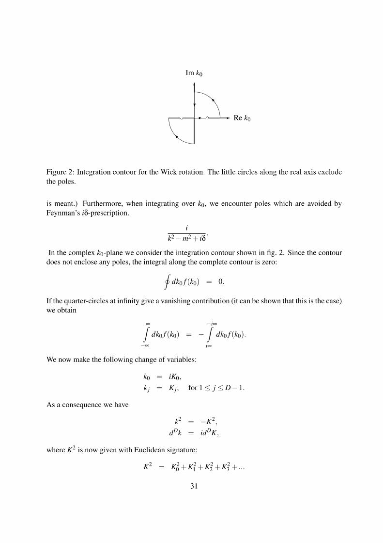
Im k0
Figure 2: Integration contour for the Wick rotation. The little circles along the real axis exclude
the poles.
is meant.) Furthermore, when integrating over k0, we encounter poles which are avoided by
Feynman’s iδ-prescription.
i
k2 −m2 + iδ.
In the complex k0-plane we consider the integration contour shown in fig. 2. Since the contour
does not enclose any poles, the integral along the complete contour is zero:
∮dk0 f (k0) = 0.
If the quarter-circles at infinity give a vanishing contribution (it can be shown that this is the case)
we obtain
∞∫
−∞
dk0 f (k0) = −−i∞∫
i∞
dk0 f (k0).
We now make the following change of variables:
k0 = iK0,
k j = K j, for 1 ≤ j ≤ D−1.
As a consequence we have
k2 = −K2,
dDk = idDK,
where K2 is now given with Euclidean signature:
K2 = K20 +K2
1 +K22 +K2
3 + ...
31

Combining the exchange of the integration contour with the change of variables we obtain for
the integration of a function f (k2) over D dimensions
∫dDk
iπD/2f (−k2) =
∫dDK
πD/2f (K2),
whenever there are no poles inside the contour of fig. 2 and the arcs at infinity give a vanishing
contribution. The integral on the r.h.s. is now over D-dimensional Euclidean space. This equation
justifies our conventions, to introduce a factor i in the denominator and a minus sign for each
propagator in the defintion of the basic scalar integrals. These conventions are just such that after
Wick rotation we have simple formulae.
4.2.4 Generalised spherical coordinates
We now have an integral over D-dimensional Euclidean space, where the integrand depends only
on K2. It is therefore natural to introduce spherical coordinates. In D dimensions they are given
by
K0 = K cosθ1,
K1 = K sinθ1 cosθ2,
...
KD−2 = K sinθ1...sinθD−2 cosθD−1,
KD−1 = K sinθ1...sinθD−2 sinθD−1.
In D dimensions we have one radial variable K, D−2 polar angles θ j (with 1 ≤ j ≤ D−2) and
one azimuthal angle θD−1. The measure becomes
dDK = KD−1dKdΩD,
where
dΩD =D−1
∏i=1
sinD−1−i θi dθi.
Integration over the angles yields
∫dΩD =
π∫
0
dθ1 sinD−2 θ1...
π∫
0
dθD−2 sinθD−2
2π∫
0
dθD−1 =2πD/2
Γ(
D2
) ,
where Γ(x) is Euler’s gamma function. Note that the integration on the l.h.s of the equation above
is defined for any natural number D, whereas the result on the r.h.s is an analytic function of D,
which can be continued to any complex value.
32

4.2.5 Euler’s gamma and beta functions
It is now the appropriate place to introduce two special functions, Euler’s gamma and beta func-
tions, which are used within dimensional regularisation to continue the results from integer D
towards non-integer values. The gamma function is defined for Re(x)> 0 by
Γ(x) =∫ ∞
0e−ttx−1dt.
It fulfils the functional equation
Γ(x+1) = x Γ(x).
For positive integers n it takes the values
Γ(n+1) = n! = 1 ·2 ·3 · ... ·n.
At x = 1/2 it has the value
Γ
(1
2
)
=√
π,
which can also be inferred from the relation
Γ(x)Γ(1− x) =π
sinπx.
For integers n we have the reflection identity
Γ(x−n)
Γ(x)= (−1)n Γ(1− x)
Γ(1− x+n).
The gamma function Γ(x) has poles located on the negative real axis at x = 0,−1,−2, .... Quite
often we will need the expansion around these poles. This can be obtained from the expansion
around x = 1 and the functional equation. The expansion around ε = 1 reads
Γ(1+ ε) = exp
(
−γEε+∞
∑n=2
(−1)n
nζnεn
)
,
where γE is Euler’s constant
γE = limn→∞
(n
∑j=1
1
j− lnn
)
= 0.5772156649...
and ζn is given by
ζn =∞
∑j=1
1
jn.
33

For example we obtain for the Laurent expansion around ε = 0
Γ(ε) =1
ε− γE +O(ε).
Euler’s beta function is defined for Re(x)> 0 and Re(y)> 0 by
B(x,y) =
1∫
0
tx−1(1− t)y−1dt,
or equivalently by
B(x,y) =
∞∫
0
tx−1
(1+ t)x+ydt.
The beta function can be expressed in terms of Gamma functions:
B(x,y) =Γ(x)Γ(y)
Γ(x+ y).
4.2.6 Result for the momentum integration
We are now in a position to perform the integration over the loop momentum. Let us discuss
again the example from the beginning of this section. After Wick rotation we have
I =
∫dDk1
iπD/2
1
(−k21)(−k2
2)(−k23)
= 2
∫dDK
πD/2
∫d3x
δ(1− x1 − x2 − x3)
(K2 − x1x2s12 − x1x3s123)3.
Introducing spherical coordinates and performing the angular integration this becomes
I =2
Γ(
D2
)
∞∫
0
dK2∫
d3xδ(1− x1 − x2 − x3)
(K2)D−2
2
(K2 − x1x2s12 − x1x3s123)3.
For the radial integration we have after the substitution t = K2/(−x1x2s12 − x1x3s123)
∞∫
0
dK2
(K2)D−2
2
(K2 − x1x2s12 − x1x3s123)3
= (−x1x2s12 − x1x3s123)D2 −3
∞∫
0
dtt
D−22
(1+ t)3.
The remaining integral is just the second definition of Euler’s beta function
∞∫
0
dtt
D−22
(1+ t)3=
Γ(
D2
)Γ(3− D
2
)
Γ(3).
34

Putting everything together and setting D = 4−2ε we obtain
∫dDk1
iπD/2
1
(−k21)(−k2
2)(−k23)
=
Γ(1+ ε)∫
d3x δ(1− x1 − x2 − x3) x−1−ε1 (−x2s12 − x3s123)
−1−ε .
Therefore we succeeded in performing the integration over the loop momentum k at the expense
of introducing a two-fold integral over the Feynman parameters.
As the steps discussed above always occur in any loop integration we can combine them into
a master formula. If U and F are functions, which are independent of the loop momentum, we
have for the integration over Minkowski space with dimension D = 2m− 2ε (with m being an
integer and ε being the dimensional regularisation parameter):
∫d2m−2εk
iπm−ε
(−k2)a
[−Uk2 +F ]ν =
Γ(m+a− ε)
Γ(m− ε)
Γ(ν−m−a+ ε)
Γ(ν)
U−m−a+ε
F ν−m−a+ε.
The functions U and F depend usually on the Feynman parameters and the external momenta
and are obtained after Feynman parametrisation from completing the square. They are however
independent of the loop momentum k. In the equation above we allowed additional powers
(−k2)a of the loop momentum in the numerator. This is a slight generalisation and will be useful
later. Here we observe that the dependency of the result on a, apart from a factor Γ(m+ a−ε)/Γ(m− ε), occurs only in the combination m+ a− ε = D/2+ a. Therefore adding a power
of (−k2) to the numerator is almost equivalent to consider the integral without this power in
dimensions D+2.
There is one more generalisation: Sometimes it is convenient to decompose k2 into a (2m)-dimensional piece and a remainder:
k2(D) = k2
(2m)+ k2(−2ε).
If D is an integer greater than 2m we have
k2(2m) = k2
0 − k21 − ...− k2
2m−1,
k(−2ε) = −k22m − ...− k2
D−1.
We also need loop integrals where additional powers of (−k2(−2ε)) appear in the numerator. These
are related to integrals in higher dimensions as follows:
∫d2m−2εk
iπm−ε(−k2
(−2ε))r f (k
µ
(2m),k2(−2ε)) =
Γ(r− ε)
Γ(−ε)
∫d2m+2r−2εk
iπm+r−εf (k
µ2m,k
2−2ε).
Here, f (kµ
(2m),k2(−2ε)) is a function which depends on k2m, k2m+1, ..., kD−1 only through k2
(−2ε).
The dependency on k0, k1, ..., k2m−1 is not constrained.
Finally it is worth noting that
∫d2m−2εk
iπm−ε
(−k2
)a=
(−1)a Γ(a+1), if m+a− ε = 0,0, otherwise.
35
4.3 Performing the Feynman integrals
Let us summarise what we learned up to now: We had the following cooking recipe for loop
integrals: In order to perform the momentum integration we proceed by the following steps:
1. Feynman parametrisation
2. Shift of the loop momentum, such that the denominator has the form(−ck2 −L
)n.
3. Wick rotation
4. Introduce generalised spherical coordinates
5. The angular integration is trivial. Using the definitions of the gamma- and beta-functions,
the radial integration can be performed.
6. This leaves only the non-trivial integration over the Feynman parameters.
We may summarise steps (3)− (5) in a master formula for the integration over the momenta in
D = 2m−2ε dimensions:
∫d2m−2εk
(2π)2m−2εi
(−k2)a
[−Uk2 +F ]n =
1
(4π)m−ε
Γ(m+a− ε)
Γ(m− ε)
Γ(n−m−a+ ε)
Γ(n)
U−m−a+ε
F n−m−a+ε
Let us now look at a few specific Feynman integrals.
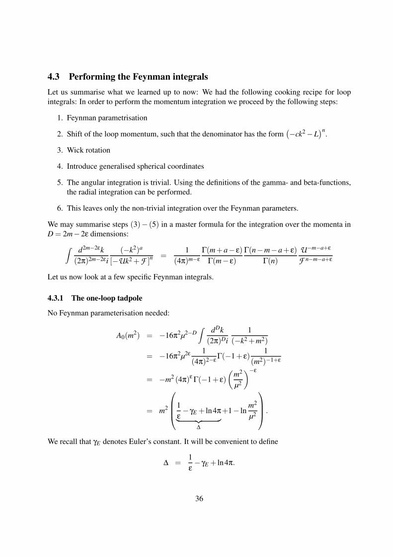
4.3.1 The one-loop tadpole
No Feynman parameterisation needed:
A0(m2) = −16π2µ2−D
∫dDk
(2π)Di
1
(−k2 +m2)
= −16π2µ2ε 1
(4π)2−εΓ(−1+ ε)
1
(m2)−1+ε
= −m2 (4π)ε Γ(−1+ ε)
(m2
µ2
)−ε
= m2
1
ε− γE + ln4π
︸ ︷︷ ︸
∆
+1− lnm2
µ2
.
We recall that γE denotes Euler’s constant. It will be convenient to define
∆ =1
ε− γE + ln4π.
36

4.3.2 The one-loop two-point function
B0(p2,m21,m
22) = 16π2µ4−D
∫dDk
(2π)Di
1(−k2 +m2
1
)(−(k− p)2 +m2
2
)
= 16π2µ4−D
1∫
0
da
∫dDk
(2π)Di
1[−k2 +a(1−a)(−p2)+am2
1 +(1−a)m22
]2
= 16π2µ2ε Γ(ε)
(4π)2−ε
1∫
0
da[a(1−a)(−p2)+am2
1+(1−a)m22
]−ε
= (4π)εµ2εΓ(ε)
1∫
0
da[a(1−a)(−p2)+am2
1+(1−a)m22
]−ε
The case m21 = m2
2 = 0:
B0(p2,0,0) = (4π)εµ2εΓ(ε)
1∫
0
da[a(1−a)(−p2)
]−ε
= (4π)εΓ(ε)
(−p2
µ2
)−ε 1∫
0
da a−ε(1−a)−ε
= (4π)εΓ(ε)
(−p2
µ2
)−εΓ(1− ε)Γ(1− ε)
Γ(2−2ε)
=1
ε− γE + ln4π+2− ln
−p2
µ2.
The case m21 = m2
2 = m 6= 0:
B0(p2,m2,m2) = (4π)εµ2εΓ(ε)
1∫
0
da[a(1−a)(−p2)+m2
]−ε
= (4π)ε
(m2
µ2
)−ε
Γ(ε)
1∫
0
da
[
1+a(1−a)
(−p2
m2
)]−ε
= (4π)ε
(m2
µ2
)−ε
Γ(ε)2
12∫
0
da
[
1+a(1−a)
(−p2
m2
)]−ε
With the substitution
b = 4a(1−a), a =1
2
(
1−√
1−b)
, da =db
4√
1−b
37

one obtains
B0(p2,m2,m2) = (4π)ε
(m2
µ2
)−ε
Γ(ε)1
2
1∫
0
db(1−b)−12 [1−bx]−ε , x =
p2
4m2
=1
2(4π)ε
(m2
µ2
)−ε
Γ(ε)
1∫
0
dbb−12 [1− (1−b)x]−ε
=1
2(4π)ε
(m2
µ2
)−ε
Γ(ε)(1− x)−ε
1∫
0
dbb−12 [1−bχ]−ε , χ =
−x
1− x=
p2
p2 −4m2
Using
(1− x)−c =1
Γ(c)
∞
∑n=0
Γ(n+ c)
Γ(n+1)xn
one obtains
B0(p2,m2,m2) =1
2(4π)ε
(m2
µ2
)−ε
(1− x)−ε∞
∑n=0
Γ(n+ ε)
Γ(n+1)χn
1∫
0
db bn− 12
=1
2(4π)ε
(m2
µ2
)−ε
(1− x)−ε∞
∑n=0
Γ(n+ ε)
Γ(n+1)
χn
(n+ 1
2
)
Divergent parts can only come from n = 0, therefore separate the sum into n = 0 and n > 0. If
we are only interested up to the finite terms, we can set ε = 0 in the n > 0 part.
B0(p2,m2,m2) = (4π)ε
(m2
µ2
)−ε
Γ(ε)(1− x)−ε +1
2
∞
∑n=1
χn
n(n+ 1
2
)
=
(1
ε− γE + ln4π− ln
m2
µ2− ln(1− x)
)
+∞
∑n=1
(
1
n− 1(n+ 1
2
)
)
χn
We further have
∞
∑n=1
χn
n= − ln(1−χ) ,
∞
∑n=1
χn
(n+ 1
2
) =∞
∑n=1
2√
χ2n
(2n+1)=
∞
∑j=1
(√χ) j+(−√
χ) j
( j+1)
= −2+1√χ
∞
∑j=1
(√χ) j
j− 1√
χ
∞
∑j=1
(−√
χ) j
j=−2− 1√
χln(1−√
χ)+1√χ
ln(1+√
χ)
38

The case m21 = m2 6= 0,m2
2 = 0:
B0(p2,m2,0) = (4π)εµ2εΓ(ε)
1∫
0
da a−ε[(1−a)(−p2)+m2
]−ε
= (4π)ε
(m2 − p2
µ2
)−ε
Γ(ε)
1∫
0
da a−ε [1−ay]−ε , y =−p2
m2 − p2
= (4π)ε
(m2 − p2
µ2
)−ε ∞
∑n=0
Γ(n+ ε)
Γ(n+1)yn
1∫
0
da an−ε
= (4π)ε
(m2 − p2
µ2
)−ε ∞
∑n=0
Γ(n+ ε)
Γ(n+1)
yn
(n+1− ε)
= (4π)ε
(m2 − p2
µ2
)−εΓ(ε)
(1− ε)+
∞
∑n=1
yn
n(n+1)
=
(1
ε− γE + ln4π+1− ln
(m2 − p2
µ2
))
+1+1− y
yln(1− y)
=1
ε− γE + ln4π+2− ln
(m2 − p2
µ2
)
− m2
p2ln
(m2
m2 − p2
)
4.3.3 More general methods
More complicated integrals are one-loop integrals with more external legs as for example the
one-loop three-point function
C0(p21, p2
2, p23,m
21,m
22,m
23) =
−16π2µ4−D∫
dDk
(2π)Di
1(−k2 +m2
1
)(−(k− p1)2 +m2
2
)(−(k− p1 − p2)2 +m2
3
)
or, in general, integrals with two or even more loops. Methods to tackle these integrals are
- Mellin-Barnes representation
- Nested sums
- Differential equations
- Sector decomposition
4.4 Tensor integrals and Passarino-Veltman reduction
We now consider the reduction of tensor loop integrals (e.g. integrals, where the loop momentum
appears in the numerator) to a set of scalar loop integrals (e.g. integrals, where the numerator is
39

independent of the loop momentum). The loop momentum appears in the numerator for example
through the Feynman rules for the quark propagator
ip/+m
p2 −m2
or the Feynman rule for the three-gluon vertex
g f abc[(k2 − k3)µgνλ +(k3 − k1)νgλµ +(k1 − k2)λgµν
]
For one-loop integrals a systematic algorithm has been first worked out by Passarino and Velt-
man. The notation for tensor integrals:
B0,µ,µν(p,m1,m2) = 16π2µ4−D∫
dDk
(2π)Di
1,kµ,kµkν
(k2 −m21)((k+ p)2−m2
2),
C0,µ,µν(p1, p2,m1,m2,m3) = 16π2µ4−D
∫dDk
(2π)Di
1,kµ,kµkν
(k2 −m21)((k+ p1)2 −m2
2)((k+ p1 + p2)2 −m23).
The reduction technique according to Passarino and Veltman consists in writing the tensor inte-
grals in the most general form in terms of form factors times external momenta and/or the metric
tensor. For example
Bµ = pµB1
Bµν = pµ pνB21 +gµνB22
Cµ = pµ1C11 + p
µ2C12
Cµν = pµ1 pν
1C21 + pµ2 pν
2C22 +p1 p2µνC23 +gµνC24
with
p1 p2µν = pµ1 pν
2 + pν1 p
µ2
One then solves for the form factors B1, B21, B22, C11, etc. by first contracting both sides with
the external momenta and the metric tensor gµν. On the left-hand side the resulting scalar prod-
ucts between the loop momentum kµ and the external momenta are rewritten in terms of the
propagators, as for example
2p · k = (k+ p)2 − k2 − p2.
The first two terms of the right-hand side above cancel propagators, whereas the last term does
not involve the loop momentum anymore. The remaining step is to solve for the formfactors by
inverting the matrix which one obtains on the right-hand side of equation (1).
40

p1
k2
Figure 3: An example for irreducible scalar products in the numerator: The scalar product 2p1k2
cannot be expressed in terms of inverse propagators.
Example for the two-point function: Contraction with pµ or pµ pν and gµν yields
p2B1 =1
2
(A0(m1)−A0(m2)+
(m2
2 −m21 − p2
)B0
)
(p2 1
p2 D
)(B21
B22
)
=
(12A0(m2)+
12(m2
2 −m21 − p2)B1
A0(m2)+m21B0
)
Solving for the form factors we obtain
B1 =1
2p2
(A0(m1)−A0(m2)+
(m2
2 −m21 − p2
)B0
)
B21 =1
6p2
(
2A0(m2)−2m21B0 +4(m2
2 −m21 − p2)B1 +(
1
3p2 −m2
1 −m22)
)
B22 =1
6
(
A0(m2)+2m21B0 − (m2
2 −m21 − p2)B1 − (
1
3p2 −m2
1 −m22)
)
Due to the matrix inversion in the lasr step Gram determinants usually appear in the denominator
of the final expression. For a three-point function we would encounter the Gram determinant of
the triangle
∆3 = 4
∣∣∣∣
p21 p1 · p2
p1 · p2 p22
∣∣∣∣.
One drawback of this algorithm is closely related to these determinants : In a phase space region
where p1 becomes collinear to p2, the Gram determinant will tend to zero, and the form factors
will take large values, with possible large cancellations among them. This makes it difficult to
set up a stable numerical program for automated evaluation of tensor loop integrals.
The Passarino-Veltman algorithm is based on the observation, that for one-loop integrals a scalar
product of the loop momentum with an external momentum can be expressed as a combination
of inverse propagators. This property does no longer hold if one goes to two or more loops. Fig.
(3) shows a two-loop diagram, for which the scalar product of a loop momentum with an external
momentum cannot be expressed in terms of inverse propagators.
41

5 Renormalisation
Recall: Loop diagrams are divergent !
∫d4k
(2π)4
1
(k2)2=
1
(4π)2
∞∫
0
dk2 1
k2=
1
(4π)2
∞∫
0
dx
x
This integral diverges at
• k2 → ∞ (UV-divergence) and at
• k2 → 0 (IR-divergence).
Use dimensional regularisation to regulate UV- and IR-divergences.
Recall the scalar one-loop two-point function for m21 = m2
2 = 0:
B0(p2,0,0) =1
ε− γE + ln4π+2− ln
−p2
µ2.
Infrared divergences cancel by summing over degenerate states. Ultraviolet divergences are ab-
sorbed into a redefinition of the parameters. Example: The renormalisation of the coupling:
gbare︸︷︷︸
divergent
= Zg︸︷︷︸
divergent
· gren︸︷︷︸
finite
.
The renormalisation constant Zg absorbs the divergent part. However Zg is not unique: One may
always shift a finite piece from gren to Zg or vice versa. Different choices for Zg correspond to
different renormalisation schemes. Two different renormalisation schemes are always connected
by a finite renormalisation. Note that different renormalisation schemes give numerically differ-
ent answers. Therefore one always has to specify the renormalisation scheme.
Some popular renormalisation schemes:
• On-shell subtraction: Define the renormalisation constants by conditions at a scale where
the particles are on-shell p2 = m2.
42

• Off-shell subtraction: For massless particles the renormalisation constants in the on-shell
scheme would contain an infrared singularity. Therefore, in the off-shell scheme one
defines the renormalisation constants by conditions at an unphysical (space-like) scale
p2 =−λ2. This scheme is also called momentum-space subtraction scheme.
• Minimal subtraction: The minimal subtraction scheme absorbs exactly the poles in 1/εinto the renormaliztion constants (and nothing else).
• Modified minimal subtraction: As Euler’s constant γE and ln(4π) always appear in combi-
nation with a pole 1/ε, the modified minimal subtraction absorbs always the combination
∆ =1
ε− γE + ln4π
into the renormaliztion constants.
5.1 Renormalisation in practice
The modified minimal subtraction is popular in QCD. The Lagrange density of QCD reads
LQCD = ∑quarks
ψ(iγµDµ −m
)ψ− 1
4Fa
µνFaµν − 1
2ξ
(∂µAa
µ
)2+ ca(x)
(
−∂µDabµ
)
cb(x),
Faµν = ∂µAa
ν −∂νAaµ +g f abcAb
µAcν,
Dµ = ∂µ − igT aAaµ,
Dabµ = ∂µ −g f abcAc
µ.
The Lagrange density depends on the (unrenormalised) fields Aaµ, ψ, ca and the (unrenormalised)
parameters g, m and ξ. We redefine the fields as follows:
Aaµ =
√
Z3Aaµ,r, ψ =
√Z2ψr, ca =
√
Z3car .
We redefine the parameters as follows:
g = Zggr, m = Zmmr, ξ = Zξξr = Z3ξr.
Substituting these relations into the Lagrange density we obtain
LQCD = Lrenorm +Lcounterterms,
where Lrenorm is given by LQCD where all bare quantities are replaced by renormalised ones. The
counterterms are given by
Lcounterterms = (Z2 −1) ψr
(iγµ∂µ
)ψr − (Z2Zm −1)mrψrψr
+(Z3 −1)1
2Aa
µ,r
(gµν∂2 −∂µ∂ν
)Ab
ν,r −(Z3 −1
)ca
r ∂2car
43

−
ZgZ
32
3︸ ︷︷ ︸
Z1
−1
gr f abc
(∂µAa
ν,r
)Ab
µ,rAcν,r −
Z2
gZ23
︸︷︷︸
Z4
−1
1
4g2
r f abe f cdeAaµ,rA
bν,rA
cµ,rA
dν,r
+
ZgZ2
√
Z3︸ ︷︷ ︸
Z1F
−1
grψrT
aγµAaµ,rψr −
ZgZ3
√
Z3︸ ︷︷ ︸
Z1
−1
gr f abc (∂µca
r )cbr Ac
µ,r.
The the various constants are not independent, but satisfy
Z1
Z3=
Z1
Z3
=Z1F
Z2=
Z4
Z1= Zg
√
Z3.
These are the Slavnov-Taylor-identities (or Ward-Takahashi identities). As a consequence, the
coupling constant renormalisation constant may be computed from the corrections to the three-
gluon-vertex, the four-gluon-vertex, the quark-gluon-vertex or the ghost-gluon vertex. The Slavnov-
Taylor identities guarantees that the result is the same.
5.1.1 Renormalisation of the coupling constant
Let g be the unrenormalised coupling constant, gr the renormalised coupling constant and gR the
dimensionless renormalised coupling constant. They are related by
g = Zggr,
gr = gRµε.
From a one-loop calculation one obtains
Zg = 1− 1
6
(11CA −4TRN f
) g2R
(4π)2∆+O(g4
R) = 1− 1
2β0
g2R
(4π)2∆+O(g4
R),
where as usual
∆ =1
ε− γE + ln(4π)
and the coulor factors are
CA = N, CF =N2 −1
2N, TR =
1
2.
β0 is given by
β0 =11
3CA −
4
3TRN f .
The unrenormalised coupling constant g is of course independent of µ:
d
dµg = 0
44

Therefore
µd
dµ(ZgµεgR) = 0,
µd
dµ(Zg)µεgR +µ
d
dµ(µε)ZggR +µ
d
dµ(gR)Zgµε = 0.
Let us define
β(gR) = µd
dµgR.
Then
β(gR) = −µ−εZ−1g µ
d
dµ(µε)ZggR −µ−εZ−1
g µd
dµ(Zg)µεgR
= −εgR −(
Z−1g µ
d
dµZg
)
gR.
Note that the first coefficient of the β-function is calculated as follows:
Z−1g µ
d
dµZg = Z−1
g µd
dµ
(
1− 1
2β0
g2R
(4π)2∆
)
= Z−1g
(−β0∆)
(4π)2gRµ
d
dµgR
= Z−1g
(−β0∆)
(4π)2gR (−εgR)
= Z−1g β0
g2R
(4π)2
= β0g2
R
(4π)2.
Therefore
β(gR) = µd
dµgR =−εgR −β0
g3R
(4π)2.
As usual denote
αs =g2
R
4π.
We then have
µ2 d
dµ2αs =
1
2µ
d
dµαs =
gR
4πµ
d
dµgR
=gR
4π
(
−εgR −β0g3
R
(4π)2
)
= −εαs −β0α2
s
4π.
45

Going to D = 4 we have therefore
µ2 d
dµ2
αs
4π= −β0
(αs
4π
)2
.
At LO the exact solution is given by
αs(µ)
4π=
1
β0 ln(
µ2
Λ2
) ,
or by
αs(µ)
4π=
αs(µ0)
4π
1
1+ αs(µ0)4π β0 ln
(µ2
µ20
) ,
depending on the preferred choice of boundary condition (Λ or αs(µ0)).
5.1.2 Mass renormalisation
As an example we consider massive quarks. The quark self-energy is given by the following
diagram:
p k1
k0
−iΣ = g2CF
∫dDk
(2π)Diγρ
i
k/1 −miγρ−i
k20
= −ig2
(4π)2CF
(1− ε)
[1
p2A0(m
2)−(
1+m2
p2
)
B0(p2,m2,0)
]
p/+4m
(
1− 1
2ε
)
B0(p2,m2,0)
= −iAp/+Bm
Resummed:
i
p/−m+
i
p/−m(−iΣ)
i
p/−m+
i
p/−m
[
(−iΣ)i
p/−m
]2
=i
p/−m
1(
1− Σp−m
) =i
p/−m−Σ
46
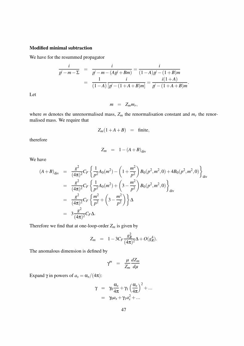
Modified minimal subtraction
We have for the resummed propagator
i
p/−m−Σ=
i
p/−m− (Ap/+Bm)=
i
(1−A)p/− (1+B)m
=1
(1−A)
i
[p/− (1+A+B)m]=
i(1+A)
p/− (1+A+B)m.
Let
m = Zmmr,
where m denotes the unrenormalised mass, Zm the renormalisation constant and mr the renor-
malised mass. We require that
Zm(1+A+B) = finite,
therefore
Zm = 1− (A+B)div
We have
(A+B)div =g2
(4π)2CF
1
p2A0(m
2)−(
1+m2
p2
)
B0(p2,m2,0)+4B0(p2,m2,0)
div
=g2
(4π)2CF
1
p2A0(m
2)+
(
3− m2
p2
)
B0(p2,m2,0)
div
=g2
(4π)2CF
m2
p2+
(
3− m2
p2
)
∆
= 3g2
(4π)2CF∆.
Therefore we find that at one-loop-order Zm is given by
Zm = 1−3CFg2
R
(4π)2∆+O(g4
R).
The anomalous dimension is defined by
γm =µ
Zm
dZm
dµ
Expand γ in powers of as = αs/(4π):
γ = γ0αs
4π+ γ1
(αs
4π
)2
+ ...
= γ0as + γ1a2s + ...
47

The first coefficients is then given by
γm0 = 6CF .
The running mass:
µd
dµm = 0.
Therefore
µ2 d
dµ2mr = −1
2γmmr =−1
2γm
0
αs
4πmr.
With
µ2 d
dµ2= −β0
(αs
4π
)2 d
d αs
4π
we find
αsd
dαs
mr =γ0
2β0mr.
Therefore
mr(µ) =
(αs(µ)
αs(µ0)
) γ02β0
mr(µ0).
The on-shell scheme
Recall that we had for the resummed propagator
i
p/−m−Σ
with
Σ = A(p2)p/+B(p2)m
Note that A(p2) and B(p2) are functions of p2. Expand Σ:
Σ(p/) = Σ|p/=mr+(p/−mr)
∂
∂p/Σ
∣∣∣∣
p/=mr︸ ︷︷ ︸
Σ′
+...
Then
i
p/−m0 −Σ=
i
p/−mr − (p/−mr)Σ′+mr −m0 −Σ|mr
=i
(1−Σ′)(p/−mr)+(mr −m0 −Σ|mr)
︸ ︷︷ ︸
=0
.
48

On-shell condition:
mr −m0 −Σ|mr= 0,
with m0 = Zmmr:
Zm = 1− 1
mr
Σ|mr
Then
i
p/−m0 −Σ=
i(1+Σ′)p/−mr
.
Calculation of Σ|p/=mr:
Σ|p/=mr= A(m2)m+B(m2)m, p/= m+(p/−m)
︸ ︷︷ ︸
can be neglected
=g2
(4π)2CF
(1− ε)
[1
m2A0(m
2)−2B0(m2,m2,0)
]
m+4m
(
1− 1
2ε
)
B0(m2,m2,0)
With
A0(m2) = m2
(
∆+1− lnm2
µ2
)
,
B0(m2,m2,0) = ∆+2− ln
m2
µ2,
one finds
Σ|p/=mr=
g2
(4π)2CF
(
−∆−2+ lnm2
µ2
)
m+4m
(
∆+3
2− ln
m2
µ2
)
= mg2
(4π)2CF
3∆+4−3lnm2
µ2
.
Therefore
Zm = 1− 1
mrΣ|mr
= 1− αs
4πCF
(
3∆+4−3lnm2
µ2
)
.
Calculation of Σ′:
Σ′ =∂
∂p/Σ
∣∣∣∣
p/=mr
=∂
∂p/
(A(p2)p/+B(p2)m
)∣∣∣∣
p/=mr
= A(m2)+ p/∂
∂p/A(p2)
∣∣
p/=mr+m
∂
∂p/B(p2)
∣∣
p/=mr
49

= A(m2)+2p/p/∂
∂p2A(p2)
∣∣
p/=mr+2mp/
∂
∂p2B(p2)
∣∣
p/=mr
= A(m2)+2m2 ∂
∂p2A(p2)
∣∣
p2=m2r+2m2 ∂
∂p2B(p2)
∣∣
p2=m2r+ ..., p/= m+(p/−m)
︸ ︷︷ ︸
can be neglected
= A(m2)+2m2 ∂
∂p2
(A(p2)+B(p2)
)∣∣
p2=m2r
We keep the Feynman parameter integral, differentiate, do the integral and expand in the end in
ε:
Σ′ =g2
(4π)2CF
(
−3
ε+3γE −3ln4π−4+3ln
m2
µ2
)
The propagator is a two-point Green function
G2(p) ∼ 〈0 |T ψψ|0〉
Under field renormalisation
ψ =√
Z2ψr
we have
G2(p)bare =(√
Z2
)2G2(p)r
Therefore
G2(p)r =iZ−1
2 (1+Σ′)p/−mr
The residue of the propagator has to be 1, therefore
Z2 = 1+Σ′ = 1+αs
4πCF
(
−3∆−4+3lnm2
µ2
)
.
50

5.2 Renormalisation to all orders
5.2.1 Power counting
The superficial degree of divergence is given by
d · l+∑v
δv −2nB −nF
where d is the dimension of space-time, l is the number of loops, δv is the number of momentum
factors at the vertex v in the diagram G, nB is the number of internal boson lines and nF is the
number of internal fermion lines.
Power counting theorem: The Feynman integral IG for the diagram G is absolutely convergent if
the superficial degree of divergence is negative for all subdiagrams H of G (including the case
H = G).
Nested, overlapping and disjoint
If a diagram H1 is completely included in H2 as a subdiagram (H1 ⊆ H2) we say that H1 is nested
in H2. If they are not included in each other but have common internal lines and vertices, they are
said to overlap. The union H1 ∪H2 is called the overlapping diagram. If they are neither nested
in each other nor overlapping (H1 ∩H2 = /0), they are said to be disjoint.
Renormalizability
The BPHZ-method (Bogoliubov and Parasiuk, Acta Math 97, 1957, 227; Hepp, Comm. Math.
Phys. 2, 1966, 301; Zimmermann, Comm. Math. Phys. 15, 1969, 208): In dimensional regular-
izion a Feynman diagram is given as a Laurent series
IG =∞
∑j=−l
a jεj
where l is a positive integer less or equal the number of loops in G. Define an operator TG for a
diagram, which picks out the divergent part, by
TGIG =−1
∑j=−l
a jεj
Define Bogoliubov’s R-operation by
RG = (1−TG) ∏H∈Φ
(1−TH)
where Φ is a set of all one-particle irreducible subdiagrams H of G, which are superficially diver-
gent. A one-particle irreducible (or proper) subdiagram H of G, which is superficially divergent
51

is also called a renormalisation part. If H1 ⊂ H2 the order is such that 1−TH1comes to the right
of 1−TH2.
Lemma on overlapping divergences: If two renormalisation parts H1 and H2 of G overlap with
each other, we have
(1−TH12)TH1
TH2= 0
for all suitable renormalisation parts H12 of G which includes both H1 and H2 as subdiagrams.
5.2.2 Hopf algebras
Let R be a commutative ring with unit 1. An algebra over the ring R is a R-module together with
a multiplication · and a unit e. We will always assume that the multiplication is associative. In
physics, the ring R will almost always be a field K (examples are the rational numbers Q, the
real numbers R or the complex number C). In this case the R-module will actually be a K-vector
space. Note that the unit can be viewed as a map from R to A and that the multiplication can
be viewed as a map from the tensor product A⊗A to A (e.g. one takes two elements from A,
multiplies them and gets one element out).
A coalgebra has instead of multiplication and unit the dual structures: a comultiplication ∆and a counit e. The counit is a map from A to R, whereas comultiplication is a map from A to A⊗A. Note that comultiplication and counit go in the reverse direction compared to multiplication
and unit. We will always assume that the comultiplication is coassociative. The general form of
the coproduct is
∆(a) = ∑i
a(1)i ⊗a
(2)i ,
where a(1)i denotes an element of A appearing in the first slot of A⊗A and a
(2)i correspondingly
denotes an element of A appearing in the second slot. Sweedler’s notation consists in dropping
the dummy index i and the summation symbol:
∆(a) = a(1)⊗a(2)
The sum is implicitly understood. This is similar to Einstein’s summation convention, except
that the dummy summation index i is also dropped. The superscripts (1) and (2) indicate that a
sum is involved.
A bialgebra is an algebra and a coalgebra at the same time, such that the two structures are
compatible with each other. Using Sweedler’s notation, the compatibility between the multipli-
cation and comultiplication is expressed as
∆(a ·b) =(
a(1) ·b(1))
⊗(
a(2) ·b(2))
.
A Hopf algebra is a bialgebra with an additional map from A to A, called the antipode S ,
which fulfills
52

A
A⊗A A⊗A
AK
∆ ·
ε η
S⊗ idid⊗S
a(1) ·S(
a(2))
= S(
a(1))
·a(2) = 0 for a 6= e.
Examples of Hopf algebras
The group algebra
Let G be a group and denote by KG the vector space with basis G. KG is an algebra with the
multiplication given by the group multiplication. The counit e is given by:
e(g) = 1.
The coproduct ∆ is given by:
∆(g) = g⊗g.
The antipode S is given by:
S (g) = g−1.
KG is a cocommutative Hopf algebra. KG is commutative if G is commutative.
Lie algebras
A Lie algebra g is not necessarily associative nor does it have a unit. To overcome this obstacle
one considers the universal enveloping algebra U(g), obtained from the tensor algebra T (g) by
factoring out the ideal
X ⊗Y −Y ⊗X − [X ,Y ] ,
with X ,Y ∈ g. The counit e is given by:
e(e) = 1, e(X) = 0.
The coproduct ∆ is given by:
∆(e) = e⊗ e, ∆(X) = X ⊗ e+ e⊗X .
The antipode S is given by:
S(e) = e, S(X) =−X .
53

Quantum SU(2)
The Lie algebra su(2) is generated by three generators H, X± with
[H,X±] =±2X±, [X+,X−] = H.
To obtain the deformed algebra Uq(su(2)), the last relation is replaced with
[X+,X−] =qH −q−H
q−q−1.
The undeformed Lie algebra su(2) is recovered in the limit q → 1. The counit e is given by:
e(e) = 1, e(H) = e(X±) = 0.
The coproduct ∆ is given by:
∆(H) = H ⊗ e+ e⊗H,
∆(X±) = X±⊗qH/2 +q−H/2 ⊗X±.
The antipode S is given by:
S(H) =−H, S(X±) =−q±1X±.
Shuffle algebras
Consider a set of letters A. A word is an ordered sequence of letters:
w = l1l2...lk.
The word of length zero is denoted by e. A shuffle algebra A on the vector space of words is
defined by
(l1l2...lk) · (lk+1...lr) = ∑shuffles σ
lσ(1)lσ(2)...lσ(r),
where the sum runs over all permutations σ, which preserve the relative order of 1,2, ...,k and of
k+1, ...,r. The counit e is given by:
e (e) = 1, e(l1l2...ln) = 0.
The coproduct ∆ is given by:
∆(l1l2...lk) =k
∑j=0
(l j+1...lk
)⊗(l1...l j
).
The antipode S is given by:
S (l1l2...lk) = (−1)k lklk−1...l2l1.
54

l
1
l
2
...
l
k1
l
k
x
0
x
1
x
2
x
3
x
4
Figure 4: An element of the shuffle algebra can be represented by a rooted tree without side-
branchings, as shown in the left figure. The right figure shows a general rooted tree with side-
branchings. The root is drawn at the top.
Rooted trees
Consider a set of rooted trees (fig. 4). An admissible cut of a rooted tree is any assignment of
cuts such that any path from any vertex of the tree to the root has at most one cut. An admissible
cut maps a tree t to a monomial in trees t1 × ...× tn+1. Precisely one of these subtrees t j will
contain the root of t. We denote this distinguished tree by RC(t), and the monomial delivered by
the n other factors by PC(t). The counit e is given by:
e(e) = 1, e(t) = 0 for t 6= e.
The coproduct ∆ is given by:
∆(e) = e⊗ e,
∆(t) = t ⊗ e+ e⊗ t + ∑adm. cuts C of t
PC(t)⊗RC(t).
The antipode S is given by:
S(e) = e,
S(t) = −t − ∑adm. cuts C of t
S(
PC(t))
×RC(t).
5.2.3 Renormalisation revisited
Short-distance singularities of the perturbative expansion of quantum field theories require renor-
malisation. The combinatorics involved in the renormalisation is governed by a Hopf algebra.
The model for this Hopf algebra is the Hopf algebra of rooted trees (fig. 5 and 6).
Recall the recursive definition of the antipode:
S(t) = −t − ∑adm. cuts C of t
S(
PC(t))
×RC(t).
The antipode satisfies
m [(S ⊗ id)∆(t)] = 0,
55

!
Figure 5: Nested singularities are encoded in rooted trees.
! +
Figure 6: Overlapping singularities yield a sum of rooted trees.
where m denotes multiplication:
m(a⊗b) = a ·b.
Let R be an operation which approximates a tree by another tree with the same singularity
structure and which satisfies the Rota-Baxter relation:
R (t1t2)+R (t1)R (t2) = R (t1R (t2))+R (R (t1) t2) .
For example, minimal subtraction (MS)
R
(∞
∑k=−L
ckεk
)
=−1
∑k=−L
ckεk
fulfills the Rota-Baxter relation. To simplify the notation, I drop the distinction between a Feyn-
man graph and the evaluation of the graph. One can now twist the antipode with R and define a
new map
SR (t) = −R
(
t + ∑adm. cuts C of t
SR
(
PC(t))
×RC(t)
)
.
From the multiplicativity constraint it follows that
SR (t1t2) = SR (t1)SR (t2) .
If we replace S by SR we obtain
m[(
SR ⊗ id)
∆(t)]
= finite,
56

since by definition SR differs from S only by finite terms. The formula above is equivalent to the
forest formula. It should be noted that R is not unique and different choices for R correspond to
different renormalisation prescription.
57

6 Mathematical structures of loop integrals
Recall: Shuffle algebras Consider a set of letters A. A word is an ordered sequence of letters:
w = l1l2...lk.
The word of length zero is denoted by e. A shuffle algebra A on the vector space of words is
defined by
(l1l2...lk) · (lk+1...lr) = ∑shuffles σ
lσ(1)lσ(2)...lσ(r),
where the sum runs over all permutations σ, which preserve the relative order of 1,2, ...,k and of
k+1, ...,r. The counit e is given by:
e (e) = 1, e(l1l2...ln) = 0.
The coproduct ∆ is given by:
∆(l1l2...lk) =k
∑j=0
(l j+1...lk
)⊗(l1...l j
).
The antipode S is given by:
S (l1l2...lk) = (−1)k lklk−1...l2l1.
Recall: Feynman- and Schwinger parameterisation.
n
∏i=1
1
(−Pi)νi
=Γ(ν)
n
∏i=1
Γ(νi)
1∫
0
(n
∏i=1
dxi xνi−1i
) δ
(
1−n
∑i=1
xi
)
(
−n
∑i=1
xiPi
)ν ,
ν =n
∑i=1
νi.
1
(−k21)(−k2
2)(−k23)
= 2
1∫
0
dx1
1∫
0
dx2
1∫
0
dx3δ(1− x1 − x2 − x3)
(−x1k2
1 − x2k22 − x3k2
3
)3
= 2
1∫
0
dx1
1−x1∫
0
dx21
(−x1k2
1 − x2k22 − (1− x1 − x2)k
23
)3.
An alternative to Feynman parameters are Schwinger parameters. Here each propagator is rewrit-
ten as
1
(−P)ν=
1
Γ(ν)
∞∫
0
dx xν−1 exp(xP).
58

p1
k2
Figure 7: An example for irreducible scalar products in the numerator: The scalar product 2p1k2
cannot be expressed in terms of inverse propagators.
Therefore we obtain for our example
1
(−k21)(−k2
2)(−k23)
=
∞∫
0
dx1
∞∫
0
dx2
∞∫
0
dx3 exp(x1k2
1 + x2k22 + x3k2
3
).
Recall: Tensor reduction at one-loop with Passarino-Veltman algorithm:
2p · k = (k+ p)2 − k2 − p2.
The Passarino-Veltman algorithm is based on the observation, that for one-loop integrals a scalar
product of the loop momentum with an external momentum can be expressed as a combination
of inverse propagators. This property does no longer hold if one goes to two or more loops. Fig.
(7) shows a two-loop diagram, for which the scalar product of a loop momentum with an external
momentum cannot be expressed in terms of inverse propagators.
Recall: If U and F are functions, which are independent of the loop momentum, we have for
the integration over Minkowski space with dimension D = 2m−2ε:
∫d2m−2εk
iπm−ε
(−k2)a
[−Uk2 +F ]ν =
Γ(m+a− ε)
Γ(m− ε)
Γ(ν−m−a+ ε)
Γ(ν)
U−m−a+ε
F ν−m−a+ε.
6.1 General tensor integrals
Let us now consider a tensor integral. After the change of variables for the diagonalisation of
the quadratic form, we have a polynomial in the Feynman or Schwinger parameters and the
loop momentum k in the numerator. Integrals with an odd power of a loop momentum in the
numerator vanish by symmetry, while integrals with an even power of the loop momentum can
be related by Lorentz invariance to scalar integrals:
∫dDk
iπD/2kµkν f (k2) =
1
Dgµν
∫dDk
iπD/2k2 f (k2),
∫dDk
iπD/2kµkνkρkσ f (k2) =
1
D(D+2)(gµνgρσ +gµρgνσ +gµσgνρ)
∫dDk
iπD/2(k2)2 f (k2).
59

The generalisation to arbitrary higher tensor structures is obvious. From the master formula:
a factor k2 in the numerator is equivalent (appart from prefactors) to a shift in the dimension
D → D+2. Let us introduce an operator D+, which shifts the dimension:
D+∫
dDk
iπD/2f(k2)
=
∫d(D+2)k
iπ(D+2)/2f(k2)
Shifting the loop momentum like in k′ = k− xp introduces the (Feynman or Schwinger) param-
eters x j in the numerator. For the tensor reduction it is convenient to work temporarily with
Schwinger parameters. Recall:
1
(−k2)ν=
1
Γ(ν)
∞∫
0
dx xν−1 exp(xk2).
A Schwinger parameter x in the numerator is equivalent to raising the power of the original
propagator by one unit: ν → ν+1. It is convenient to denote by i+ the operator, which raises the
power of propagator i by one.
νii+ 1(−k2
i
)νi= νi
1(−k2
i
)νi+1=
1
Γ(νi)
∞∫
0
dxi xνi−1i xi exp(xik
2).
All Schwinger integrals are rewritten in terms of these scalar integrals. Therefore, using an
intermediate Schwinger parametrisation, we have expressed all tensor integrals in terms of scalar
integrals. The price we paid is that these scalar integrals involve higher powers of the propagators
and/or have shifted dimensions. Each integral can be specified by its topology, its value for the
dimension D and a set of indices, denoting the powers of the propagators. In general the number
of different integrals is quite large.
6.2 Expansion of transcendental functions
To eliminate powers of the loop momentum in the numerator one can trade the loop momentum
in the numerator for scalar integrals (e.g. numerator = 1) with higher powers of the propagators
and shifted dimensions:
∫d2m−2εk1
(2π)2m−2ε
1(k2
1
)ν1(k2
2
)ν2(k2
3
)ν3.
In the second step an integral of type (1) is now converted into an infinite sum. Introducing
Feynman parameters, performing the momentum integration and then the integration over the
Feynman parameters one obtains
∫d2m−2εk1
iπm−ε
1
(−k21)
ν1
1
(−k22)
ν2
1
(−k23)
ν3
60

=(−p2
123
)m−ε−ν123 Γ(ν123 −m+ ε)
Γ(ν1)Γ(ν2)Γ(ν3)
1∫
0
da aν2−1(1−a)ν3−1
×1∫
0
db bm−ε−ν23−1(1−b)m−ε−ν1−1 [1−a(1− x)]m−ε−ν123
=(−p2
123
)m−ε−ν123 1
Γ(ν1)Γ(ν2)
Γ(m− ε−ν1)Γ(m− ε−ν23)
Γ(2m−2ε−ν123)
×∞
∑n=0
Γ(n+ν2)Γ(n−m+ ε+ν123)
Γ(n+1)Γ(n+ν23)(1− x)n ,
where x = p212/p2
123, ν23 = ν2 +ν3 and ν123 = ν1 +ν2 +ν3. To arrive at the last line of (1) one
expands [1−a(1− x)]m−ε−ν123 according to
(1− z)−c =1
Γ(c)
∞
∑n=0
Γ(n+ c)
Γ(n+1)zn.
Then all Feynman parameter integrals are of the form
1∫
0
da aµ−1(1−a)ν−1 =Γ(µ)Γ(ν)
Γ(µ+ν).
The infinite sum in the last line of (1) is a hypergeometric function, where the small parameter εoccurs in the Gamma-functions:
2F1(ν2,−m+ ε+ν123;ν23;1− x) =
Γ(ν23)
Γ(ν2)Γ(−m+ ε+ν123)
∞
∑n=0
Γ(n+ν2)Γ(n−m+ ε+ν123)
Γ(n+1)Γ(n+ν23)(1− x)n ,
6.3 Nested Sums
In this section I review the underlying mathematical structure for the systematic expansion of
transcendental functions like the hypergeometric function in (1). I discuss properties of particular
forms of nested sums, which are called Z-sums and show that they form a Hopf algebra. This
Hopf algebra admits as additional structures a conjugation and a convolution product. Z-sums
are defined by
Z(n;m1, ...,mk;x1, ...,xk) = ∑n≥i1>i2>...>ik>0
xi11
i1m1
. . .x
ikk
ikmk.
k is called the depth of the Z-sum and w = m1 + ...+mk is called the weight. If the sums go to
Infinity (n = ∞) the Z-sums are multiple polylogarithms:
Z(∞;m1, ...,mk;x1, ...,xk) = Lim1,...,mk(x1, ...,xk).
61

For x1 = ...= xk = 1 the definition reduces to the Euler-Zagier sums:
Z(n;m1, ...,mk;1, ...,1) = Zm1,...,mk(n).
For n = ∞ and x1 = ...= xk = 1 the sum is a multiple ζ-value:
Z(∞;m1, ...,mk;1, ...,1) = ζ(m1, ...,mk).
The multiple polylogarithms contain as the notation already suggests as subsets the classical
polylogarithms Lin(x), as well as Nielsen’s generalised polylogarithms
Sn,p(x) = Lin+1,1,...,1(x,1, ...,1︸ ︷︷ ︸
p−1
),
and the harmonic polylogarithms
Hm1,...,mk(x) = Lim1,...,mk
(x,1, ...,1︸ ︷︷ ︸
k−1
).
The usefulness of the Z-sums lies in the fact, that they interpolate between multiple polyloga-
rithms and Euler-Zagier sums.
In addition to Z-sums, it is sometimes useful to introduce as well S-sums. S-sums are defined
by
S(n;m1, ...,mk;x1, ...,xk) = ∑n≥i1≥i2≥...≥ik≥1
xi11
i1m1
. . .x
ikk
ikmk.
The S-sums reduce for x1 = ...= xk = 1 (and positive mi) to harmonic sums:
S(n;m1, ...,mk;1, ...,1) = Sm1,...,mk(n).
The S-sums are closely related to the Z-sums, the difference being the upper summation boundary
for the nested sums: (i−1) for Z-sums, i for S-sums. The introduction of S-sums is redundant,
since S-sums can be expressed in terms of Z-sums and vice versa. It is however convenient to
introduce both Z-sums and S-sums, since some properties are more naturally expressed in terms
of Z-sums while others are more naturally expressed in terms of S-sums.
The Z-sums form an algebra. The unit element in the algebra is given by the empty sum
e = Z(n).
The empty sum Z(n) equals 1 for non-negative integer n. Before I discuss the multiplication rule,
let me note that the basic building blocks of Z-sums are expressions of the form
xnj
nm j,
62

which will be called “letters”. For fixed n, one can multiply two letters with the same n:
xn1
nm1· xn
2
nm2=
(x1x2)n
nm1+m2,
e.g. the x j’s are multiplied and the degrees are added. Let us call the set of all letters the alphabet
A. As a short-hand notation I will in the following denote a letter just by X j = xnj/nm j . A word is
an ordered sequence of letters, e.g.
W = X1,X2, ...,Xk.
The word of length zero is denoted by e. The Z-sums defined in (1) are therefore completely
specified by the upper summation limit n and a word W . A quasi-shuffle algebra A on the
vectorspace of words is defined by
eW = W e =W,
(X1,W1) (X2,W2) = X1,(W1 (X2,W2))+X2,((X1,W1)W2)
+(X1 ·X2),(W1 W2).
Note that “·” denotes multiplication of letters as defined in eq. (1), whereas “” denotes the
product in the algebra A , recursively defined in eq. (1). This defines a quasi-shuffle product for
Z-sums. The recursive definition in (1) translates for Z-sums into
Zm1,...,mk(n)×Zm′
1,...,m′l(n)
=n
∑i1=1
1
im11
Zm2,...,mk(i1 −1)Zm′
1,...,m′l(i1−1)
+n
∑i2=1
1
im′
1
2
Zm1,...,mk(i2 −1)Zm′
2,...,m′l(i2 −1)
+n
∑i=1
1
im1+m′1
Zm2,...,mk(i−1)Zm′
2,...,m′l(i−1).
The proof that Z-sums obey the quasi-shuffle algebra is sketched in Fig. 8. The outermost sums
of the Z-sums on the l.h.s of (1) are split into the three regions indicated in Fig. 8. A simple
example for the multiplication of two Z-sums is
Z(n;m1;x1)Z(n;m1;x2) =
Z(n;m1,m2;x1,x2)+Z(n;m2,m1;x2,x1)+Z(n;m1+m2;x1x2).
The quasi-shuffle algebra A is isomorphic to the free polynomial algebra on the Lyndon
words. If one introduces a lexicographic ordering on the letters of the alphabet A, a Lyndon word
is defined by the property
W <V
63

-
6
i
1
i
2
=
-
6
i
1
i
2
+
-
6
i
1
i
2
+
-
6
i
1
i
2
Figure 8: Sketch of the proof for the multiplication of Z-sums. The sum over the square is
replaced by the sum over the three regions on the r.h.s.
for any subwords U and V such that W =U,V . Here U,V means just concatenation of U and V .
The Z-sums form actuall a Hopf algebra. It is convenient to phrase the coalgebra structure in
terms of rooted trees. Z-sums can be represented as rooted trees without any sidebranchings. As
a concrete example the pictorial representation of a sum of depth three reads:
Z(n;m1,m2,m3;x1,x2,x3) =n
∑i1=1
i1−1
∑i2=1
i2−1
∑i3=1
xi11
i1m1
xi22
i2m2
xi33
i3m3
=
x1
x2
x3
The outermost sum corresponds to the root. By convention, the root is always drawn on the
top. Trees with sidebranchings are given by nested sums with more than one subsum, for exam-
ple:
n
∑i=1
xi1
im1Z(i−1;m2,x2)Z(i−1;m3;x3) =
x1
x2 x3
Of course, due to the multiplication formula, trees with sidebranchings can always be reduced to
trees without any sidebranchings. The coalgebra structure is now formulated in terms of rooted
trees. I first introduce some notation how to manipulate rooted trees, following the notation of
Kreimer and Connes. An elementary cut of a rooted tree is a cut at a single chosen edge. An
admissible cut is any assignment of elementary cuts to a rooted tree such that any path from any
vertex of the tree to the root has at most one elementary cut. An admissible cut maps a tree t to a
monomial in trees t1 ... tk+1. Note that precisely one of these subtrees t j will contain the root
of t. Denote this distinguished tree by RC(t), and the monomial delivered by the k other factors
by PC(t). The counit e is given by
e(e) = 1,
e(t) = 0, t 6= e.
The coproduct ∆ is defined by the equations
∆(e) = e⊗ e,
64

∆(t) = e⊗ t + t ⊗ e+ ∑adm. cuts C of t
PC(t)⊗RC(t),
∆(t1 ... tk) = ∆(t1)(⊗)...(⊗)∆(tk).
The antipode S is given by
S(e) = e,
S(t) = −t − ∑adm. cuts C of t
S(
PC(t))
RC(t),
S(t1 ... tk) = S(t1) ...S(tk).
Since the multiplication in the algebra is commutative the antipode satisfies
S 2 = id.
Let me give some examples for the coproduct and the antipode for Z-sums:
∆Z(n;m1;x1) = e⊗Z(n;m1;x1)+Z(n;m1;x1)⊗ e,
∆Z(n;m1,m2;x1,x2) = e⊗Z(n;m1,m2;x1,x2)+Z(n;m1,m2;x1,x2)⊗ e
+Z(n;m2;x2)⊗Z(n;m1;x1),
SZ(n;m1;x1) = −Z(n;m1;x1),
SZ(n;m1,m2;x1,x2) = Z(n;m2,m1;x2,x1)+Z(n;m1 +m2;x1x2).
The Hopf algebra of nested sums has additional structures if we allow expressions of the form
xn0
nm0Z(n;m1, ...,mk;x1, ...,xk),
e.g. Z-sums multiplied by a letter. Then the following convolution product
n−1
∑i=1
xi
imZ(i−1; ...)
yn−i
(n− i)m′ Z(n− i−1; ...)
can again be expressed in terms of expressions of the form (1). An example is
n−1
∑i=1
xi
iZ1(i−1)
yn−i
(n− i)Z1(n− i−1) =
xn
n
[
Z
(
n−1;1,1,1;y
x,x
y,y
x
)
+Z
(
n−1;1,1,1;y
x,1,
x
y
)
+Z(
n−1;1,1,1;1,y
x,1)]
+(x ↔ y) .
In addition there is a conjugation, e.g. sums of the form
−n
∑i=1
(n
i
)
(−1)i xi
imS(i; ...)
65

can also be reduced to terms of the form (1). Although one can easily convert between the
notations for S-sums and Z-sums, expressions involving a conjugation tend to be shorter when
expressed in terms of S-sums. The name conjugation stems from the following fact: To any func-
tion f (n) of an integer variable n one can define a conjugated function C f (n) as the following
sum
C f (n) =n
∑i=1
(n
i
)
(−1)i f (i).
Then conjugation satisfies the following two properties:
C 1 = 1,
C C f (n) = f (n).
An example for a sum involving a conjugation is
−n
∑i=1
(n
i
)
(−1)i xi
iS1(i) =
S
(
n;1,1;1− x,1
1− x
)
−S (n;1,1;1− x,1) .
Finally there is the combination of conjugation and convolution, e.g. sums of the form
−n−1
∑i=1
(n
i
)
(−1)i xi
imS(i; ...)
yn−i
(n− i)m′ S(n− i; ...)
can also be reduced to terms of the form (1). An example is given by
−n−1
∑i=1
(n
i
)
(−1)iS(i;1;x) S(n− i;1;y) =
1
n
S(n;1;y)+(1− x)n
[
S
(
n;1;1
1− 1x
)
−S
(
n;1;1− y
x
1− 1x
)]
+(−1)n
n
S(n;1;x)+(1− y)n
[
S
(
n;1;1
1− 1y
)
−S
(
n;1;1− x
y
1− 1y
)]
.
6.4 Expansion of hypergeometric functions
In this section I discuss how the algebraic tools introduced in the previous section can be used to
solve the problems outlined at the end of Sect. 6.2. First I give some motivation for the introduc-
tion of Z-sums: The essential point is that Z-sums interpolate between multiple polylogarithms
and Euler-Zagier-sums, such that the interpolation is compatible with the algebra structure. On
66

the one hand, we expect multiple polylogarithm to appear in the Laurent expansion of the tran-
scendental functions (1), a fact which is confirmed a posteriori. Therefore it is important that
multiple polylogarithms are contained in the class of Z-sums. On the other the expansion param-
eter ε occurs in the functions (1) inside the arguments of Gamma-functions. The basic formula
for the expansion of Gamma-functions reads
Γ(n+ ε) = Γ(1+ ε)Γ(n)[1+ εZ1(n−1)+ ε2Z11(n−1)
+ε3Z111(n−1)+ ...+ εn−1Z11...1(n−1)],
containing Euler-Zagier sums for finite n. As a simple example I discuss the expansion of
∞
∑i=0
Γ(i+a1 + t1ε)Γ(i+a2+ t2ε)
Γ(i+1)Γ(i+a3+ t3ε)xi
into a Laurent series in ε. Here a1, a2 and a3 are assumed to be integers. Up to prefactors the
expression in (1) is a hypergeometric function 2F1. Using Γ(x+1) = xΓ(x), partial fractioning
and an adjustment of the summation index one can transform (1) into terms of the form
∞
∑i=1
Γ(i+ t1ε)Γ(i+ t2ε)
Γ(i)Γ(i+ t3ε)
xi
im,
where m is an integer. Now using (1) one obtains
Γ(1+ ε)∞
∑i=1
(1+ εt1Z1(i−1)+ ...)(1+ εt2Z1(i−1)+ ...)
(1+ εt3Z1(i−1)+ ...)
xi
im.
Inverting the power series in the denominator and truncating in ε one obtains in each order in εterms of the form
∞
∑i=1
xi
imZm1...mk
(i−1)Zm′1...m
′l(i−1)Zm′′
1...m′′n(i−1)
Using the quasi-shuffle product for Z-sums the three Euler-Zagier sums can be reduced to single
Euler-Zagier sums and one finally arrives at terms of the form
∞
∑i=1
xi
imZm1...mk
(i−1),
which are harmonic polylogarithms Hm,m1,...,mk(x). This completes the algorithm for the expan-
sion in ε for sums of the form (1). Since the one-loop integral discussed in (1) is a special case
of (1), this algorithm also applies to the integral (1). In addition, this algorithm shows that in the
expansion of hypergeometric functions J+1FJ(a1, ...,aJ+1;b1, ...,bJ;x) around integer values of
the parameters ak and bl only harmonic polylogarithms appear in the result.
67

Let me come back to the example of the one-loop Feynman integral discussed in Sect. 6.2.
For ν1 = ν2 = ν3 = 1 and m = 2 in (1) one obtains:
∫d4−2εk1
iπ2−ε
1
(−k21)
1
(−k22)
1
(−k23)
=Γ(−ε)Γ(1− ε)Γ(1+ ε)
Γ(1−2ε)
(−p2
123
)−1−ε
1− x
∞
∑n=1
εn−1H1, ...,1︸ ︷︷ ︸
n
(1− x).
Here, all harmonic polylogarithms can be expressed in terms of Nielsen polylogarithms, which
in turn simplify to powers of the standard logarithm:
H1, ...,1︸ ︷︷ ︸
n
(1− x) = S0,n(1− x) =(−1)n
n!(lnx)n .
This particular example is very simple and one recovers the well-known all-order result
Γ(1− ε)2Γ(1+ ε)
Γ(1−2ε)
(−p2
123
)−1−ε
ε2
1− x−ε
1− x,
which (for this simple example) can also be obtained by direct integration.
6.5 The integral representation of multiple polylogarithms
The multiple polylogarithms are special cases of Z-sums. They are obtained from Z-sums by
taking the outermost sum to infinity:
Z(∞;m1, ...,mk;x1, ...,xk) = Lim1,...,mk(x1, ...,xk).
Being special cases of Z-sums they obey the quasi-shuffle Hopf algebra for Z-sums. Multiple
polylogarithms have been defined in this article via the sum representation (1). In addition, they
admit an integral representation. From this integral representation a second algebra structure
arises, which turns out to be a shuffle Hopf algebra. To discuss this second Hopf algebra it is
convenient to introduce for zk 6= 0 the following functions
G(z1, ...,zk;y) =
y∫
0
dt1
t1 − z1
t1∫
0
dt2
t2 − z2...
tk−1∫
0
dtk
tk − zk
.
In this definition one variable is redundant due to the following scaling relation:
G(z1, ...,zk;y) = G(xz1, ...,xzk;xy)
If one further defines
g(z;y) =1
y− z,
68

then one has
d
dyG(z1, ...,zk;y) = g(z1;y)G(z2, ...,zk;y)
and
G(z1,z2, ...,zk;y) =
y∫
0
dt g(z1; t)G(z2, ...,zk; t).
One can sligthly enlarge the set and define G(0, ...,0;y) with k zeros for z1 to zk to be
G(0, ...,0;y) =1
k!(lny)k .
This permits us to allow trailing zeros in the sequence (z1, ...,zk) by defining the function G
with trailing zeros via (1) and (1). To relate the multiple polylogarithms to the functions G it is
convenient to introduce the following short-hand notation:
Gm1,...,mk(z1, ...,zk;y) = G(0, ...,0
︸ ︷︷ ︸
m1−1
,z1, ...,zk−1,0...,0︸ ︷︷ ︸
mk−1
,zk;y)
Here, all z j for j = 1, ...,k are assumed to be non-zero. One then finds
Lim1,...,mk(x1, ...,xk) = (−1)kGm1,...,mk
(1
x1,
1
x1x2, ...,
1
x1...xk
;1
)
.
The inverse formula reads
Gm1,...,mk(z1, ...,zk;y) = (−1)k Lim1,...,mk
(y
z1,z1
z2, ...,
zk−1
zk
)
.
Eq. (1) together with (1) and (1) defines an integral representation for the multiple polyloga-
rithms. To make this more explicit I first introduce some notation for iterated integrals
Λ∫
0
dt
t −an ... dt
t −a1=
Λ∫
0
dtn
tn −an
tn∫
0
dtn−1
tn−1−an−1× ...×
t2∫
0
dt1
t1 −a1
and the short hand notation:
Λ∫
0
(dt
t)m
dt
t −a=
Λ∫
0
dt
t ...dt
t︸ ︷︷ ︸
m times
dt
t −a.
69

The integral representation for Limk,...,m1(xk, ...,x1) reads then
Lim1,...,mk(x1, ...,xk) = (−1)k
1∫
0
(dt
t)m1−1
dt
t −b1
(
dt
t)m2−1
dt
t −b2 ...
(dt
t)mk−1
dt
t −bk
,
where the b j’s are related to the x j’s
b j =1
x1x2...x j.
From the iterated integral representation (1) a second algebra structure for the functions G(z1, ...,zk;y)(and through (1) also for the multiple polylogarithms) is obtained as follows: We take the z j’s as
letters and call a sequence of ordered letters w= z1, ...,zk a word. Then the function G(z1, ...,zk;y)is uniquely specified by the word w = z1, ...,zk and the variable y. The neutral element e is given
by the empty word, equivalent to
G(;y) = 1.
A shuffle algebra on the vector space of words is defined by
ew = w e = w,
(z1,w1) (z2,w2) = z1,(w1 (z2,w2))+ z2,((z1,w1)w2).
Note that this definition is very similar to the definition of the quasi-shuffle algebra (1), except
that the third term in (1) is missing. In fact, a shuffle algebra is a special case of a quasi-shuffle
algebra, where the product of two letters is degenerate: X1 ·X2 = 0 for all letters X1 and X2 in
the notation of Sect. 6.3. The definition of the shuffle product (1) translates into the following
recursive definition of the product of two G-functions:
G(z1, ...,zk;y)×G(zk+1, ...,zn;y) =y∫
0
dt
t − z1G(z2, ...,zk; t)G(zk+1, ...,zn; t)
+
y∫
0
dt
t − zk+1
G(z1, ...,zk; t)G(zk+2, ...,zn; t)
For the discussion of the coalgebra part for the functions G(z1, ...,zk;y) we may proceed as
in Sect. 6.3 and associate to any function G(z1, ...,zk;y) a rooted tree without sidebranchings as
in the following example:
G(z1,z2,z3;y) =
z1
z2
z370

The outermost integration (involving z1) corresponds to the root. The formulae for the coproduct
(1) and the antipode (1) apply then also to the functions G(z1, ...,zk;y).A shuffle algebra is simpler than a quasi-shuffle algebra and one finds for a shuffle alge-
bra besides the recursive definitions of the product, the coproduct and the antipode also closed
formulae for these operations. For the product one has
G(z1, ...,zk;y) G(zk+1, ...,zk+l;y) = ∑shu f f le
G(zσ(1), ...,zσ(k+l);y
),
where the sum is over all permutations which preserve the relative order of the strings z1, ...,zk
and zk+1, ...,zk+l. This explains the name “shuffle product”. For the coproduct one has
∆G(z1, ...,zk;y) =k
∑j=0
G(z1, ...,z j;y)⊗G(z j+1, ...,zk;y)
and for the antipode one finds
SG(z1, ...,zk;y) = (−1)kG(zk, ...,z1;y).
The shuffle multiplication is commutative and the antipode satisfies therefore
S 2 = id.
From (1) this is evident.
6.6 The antipode and integration-by-parts
Integration-by-parts has always been a powerful tool for calculations in particle physics. By
using integration-by-parts one may obtain an identity between various G-functions. The starting
point is as follows:
G(z1, ...,zk;y) =
y∫
0
dt
(∂
∂tG(z1; t)
)
G(z2, ...,zk; t)
= G(z1;y)G(z2, ...,zk;y)−y∫
0
dt G(z1; t)g(z2; t)G(z3, ...,zk; t)
= G(z1;y)G(z2, ...,zk;y)−y∫
0
dt
(∂
∂tG(z2,z1; t)
)
G(z3, ...,zk; t).
Repeating this procedure one arrives at the following integration-by-parts identity:
G(z1, ...,zk;y)+(−1)kG(zk, ...,z1;y)
= G(z1;y)G(z2, ...,zk;y)−G(z2,z1;y)G(z3, ...,zk;y)+ ...
−(−1)k−1G(zk−1, ...z1;y)G(zk;y),
71

which relates the combination G(z1, ...,zk;y)+(−1)kG(zk, ...,z1;y) to G-functions of lower depth.
This relation is useful in simplifying expressions. Eq. (1) can also be derived in a different way.
In a Hopf algebra we have for any non-trivial element w the following relation involving the
antipode:
∑(w)
w(1) ·S(w(2)) = 0.
Here Sweedler’s notation has been used. Sweedler’s notation writes the coproduct of an element
w as
∆(w) = ∑(w)
w(1)⊗w(2).
Working out the relation (1) for the shuffle algebra of the functions G(z1, ..., zk;y), we recover
(1).
We may now proceed and check if (1) provides also a non-trivial relation for the quasi-shuffle
algebra of Z-sums. This requires first some notation: A composition of a positive integer k is a
sequence I = (i1, ..., il) of positive integers such that i1 + ...il = k. The set of all composition of
k is denoted by C (k). Compositions act on Z-sums as
(i1, ..., il)Z(n;m1, ...,mk;x1, ...,xk)
= Z(n;m1 + ...+mi1,mi1+1 + ...+mi1+i2, ...,mi1+...+il−1+1 + ...
+mi1+...+il ;x1...xi1,xi1+1...xi1+i2, ...,xi1+...+il−1+1...xi1+...+il
),
e.g. the first i1 letters of the Z-sum are combined into one new letter, the next i2 letters are
combined into the second new letter, etc.. With this notation for compositions one obtains the
following closed formula for the antipode in the quasi-shuffle algebra:
SZ(n;m1, ...,mk;x1, ...,xk) = (−1)k ∑I∈C (k)
I Z(n;mk, ...,m1;xk, ...,x1)
From (1) we then obtain
Z(n;m1, ...,mk;x1, ...,xk)+(−1)kZ(n;mk, ...,m1;xk, ...,x1)
= − ∑adm. cuts
PC(Z(n;m1, ...,mk;x1, ...,xk))
·S(
RC(Z(n;m1, ...,mk;x1, ...,xk)))
−(−1)k ∑I∈C (k)\(1,1,...,1)
I Z(n;mk, ...,m1;xk, ...,x1).
Again, the combination Z(n;m1, ...,mk;x1, ...,xk)+(−1)kZ(n;mk, ...,m1;xk, ...,x1) reduces to Z-
sums of lower depth, similar to (1). We therefore obtained an “integration-by-parts” identity for
objects, which don’t have an integral representation. We first observed, that for the G-functions,
72
which have an integral representation, the integration-by-parts identites are equal to the iden-
tities obtained from the antipode. After this abstraction towards an algebraic formulation, one
can translate these relations to cases, which only have the appropriate algebra structure, but not
necessarily a concrete integral representation. As an example we have
Z(n;m1,m2,m3;x1,x2,x3)−Z(n;m3,m2,m1;x3,x2,x1) =
Z(n;m1;x1)Z(n;m2,m3;x2,x3)−Z(n;m2,m1;x2,x1)Z(n;m3;x3)
−Z(n;m1 +m2;x1x2)Z(n;m3;x3)+Z(n;m2 +m3,m1;x2x3,x1)
+Z(n;m3,m1+m2;x3,x1x2)+Z(n;m1+m2 +m3;x1x2x3),
which expresses the combination of the two Z-sums of depth 3 as Z-sums of lower depth. The
analog example for the shuffle algebra of the G-function reads:
G(z1,z2,z3;y)−G(z3,z2,z1;y) = G(z1;y)G(z2,z3;y)−G(z2,z1;y)G(z3;y).
Multiple polylogarithms obey both the quasi-shuffle algebra and the shuffle algebra. Therefore
we have for multiple polylogarithms two relations, which are in general independent.
6.7 Numerical evaluation of multiple polylogarithms
The real part of the dilogarithm Li2(x) is numerically evaluated as follows: Using the relations
Li2(x) = −Li2(1− x)+π2
6− ln(x) ln(1− x),
Li2(x) = −Li2
(1
x
)
− π2
6− 1
2(ln(−x))2 ,
the argument is shifted into the range −1 ≤ x ≤ 1/2. Then
Li2(x) =∞
∑i=0
Bi
(i+1)!zi+1
= B0z+B1
2z2 +
∞
∑n=1
B2n
(2n+1)!z2n+1,
with z =− ln(1−x) and the Bi are the Bernoulli numbers. The Bernoulli numbers Bi are defined
through the generating function
t
et −1=
∞
∑i=0
Bntn
n!.
It is also convenient to use the Clausen function Cl2(x) as an auxilary function.
73

6.8 Mellin-Barnes integrals
(A1 +A2)−a =
1
2πi
i∞∫
−i∞
dσΓ(−σ)Γ(α+σ)
Γ(α)Aσ
1 A−α−σ2
with |arg A1 − arg A2| < π. The contour is such that the poles of Γ(−σ) (UV-poles) are to the
right and the poles of Γ(α+σ) (IR-poles) are to the left.
Closing the contour to the left:
1
2πi
∫dσ... = ∑
res
...
Closing the contour to the right (negative “umlauf” number):
1
2πi
∫dσ... = −∑
res
...
Barnes first lemma:
1
2πi
i∞∫
−i∞
dzΓ(a+ z)Γ(b+ z)Γ(c− z)Γ(d− z) =Γ(a+ c)Γ(a+d)Γ(b+ c)Γ(b+d)
Γ(a+b+ c+d)
if none of the poles of Γ(a+ z)Γ(b+ z) coincides with the ones from Γ(c− z)Γ(d− z) and if the
contour separates the increasing series of poles from the decreasing ones.
Barnes second lemma:
1
2πi
i∞∫
−i∞
dzΓ(a+ z)Γ(b+ z)Γ(c+ z)Γ(d− z)Γ(e− z)
Γ(a+b+ c+d + e+ z)
=Γ(a+d)Γ(b+d)Γ(c+d)Γ(a+ e)Γ(b+ e)Γ(c+ e)
Γ(a+b+d+ e)Γ(a+ c+d + e)Γ(b+ c+d + e)
74

7 From differential geometry to Yang-Mills theory
Additional textbooks:
- O. Forster, Analysis 3, Vieweg, (differential forms)
- M. Schottenloher, Geometrie und Symmetrie in der Physik, Vieweg,
- M. Nakahara, Geometry, Topology and Physics, Institute of Physics
7.1 Manifolds
M is an n-dimensional differentiable manifold if
• M is a topological space
• M is provided with a family of open sets Ui together with corresponding mappings ϕi,
such that the family Ui covers M, that is,
∪Ui = M
and where ϕi is a homeomorphism from Ui onto an open subset Vi ⊆ Rn.
• Given Ui and U j with Ui ∩U j 6= /0, the map ϕi j = ϕiϕ−1j from ϕ j(Ui ∩U j) to ϕi(Ui ∩U j) is
infinitely differentiable.
The pair (Ui,ϕi) is called a chart, while the whole family (Ui,ϕi) is called an atlas. The subset
Ui is called the coordinate neighbourhood while ϕi is the coordinate function or simply the coor-
dinate. Note that M is locally Euclidean and in each coordinate neighbourhood M looks like an
open subset of Rn. But note that we do not require that M be Rn globally.
A map f : X → Y between two topological spaces X and Y is called a homeomorphism if it
is continous and has an inverse f−1 : Y → X which is also continous. In that case X and Y are
said to be homeomorphic to each other.
A map f : X → Y is called a diffeomorphism if it is a homeomorphism and f i ∈C∞.
Let I ⊂ R be an interval and γ : I → M ⊂ Rn a differentiable map. A tangent vector to M at
the point γ(t0) is defined by
d
dtγ(t)
∣∣∣∣t0
∈ Rn.
The set of all tangent vectors to M at the point p is denoted by TpM. We denote by T ∗p M the dual
vector space of TpM, i.e. the set of all linear forms
φ : TpM → R.
75
Elements of φ ∈ T ∗p M are called co-tangent vectors.
A vector field is a map
X : M →Rn
X associates to each point p ∈ M a tangent vector X(p) ∈ Rn.
7.2 Differential forms
A differential form of order one is a map
ω : M →⋃p
T ∗p M
with ω(p) ∈ T ∗p M. The differential form ω associates to each point p ∈ M a co-tangent vector
ω(p) ∈ T ∗p M. We denote the value of ω(p) applied to the tangent vector v ∈ TpM by
〈ω(p),v〉
Example: Let U ⊂Rn and let f : U →R be a differentiable function. The total differential d f of
f is defined by
〈d f (p),v〉 =n
∑i=1
∂ f (p)
∂xi
vi.
Coordinate representation: Every differential form of order one can be written as
ω =n
∑i=1
fi(x)dxi.
Integrals along a curve: Let γ : [a,b]→U be a curve . The the integral of ω along γ is defined by
∫
γ
ω =
b∫
a
〈ω(γ(t),γ′(t)〉dt.
Wedge product of linear forms: Let ω1, ..., ωK ∈V ∗ denote linear forms. The wedge product is
a map
ω1 ∧ ...∧ωk : V k → R
defined by
(ω1 ∧ ...∧ωk)(v1, ...,vk) = det
〈ω1,v1〉 ... 〈ω1,vk〉... ... ...
〈ωk,v1〉 ... 〈ωk,vk〉
76

Coordinate representation of differential forms of order k:
ω =1
k!∑ fi1...ikdxi1 ∧ ...∧dxik.
Pull-back of differential forms: Let U ⊂ Rn and let
ω =1
k!∑ fi1...ikdxi1 ∧ ...∧dxik.
be a k-form in U . Further assume that an open set V ⊂ Rm and a differential map
ϕ = (ϕ1, ...,ϕn) : V →U
are given. Then it is possible to define a k-form ϕ∗ω in V by
ϕ∗ω =1
k!∑( fi1...ik ϕ)dϕi1 ∧ ...∧dϕik.
Remark: k-forms can be integrated over k-dimensional (sub-) manifolds.
Example:
A = ie
~cAµ(x)dxµ,
defines a one-form. Further
dA = d(
ie
~cAνdxν
)
= ie
~c∂µAνdxµ ∧dxν
= ie
~c
1
2
(∂µAν−∂νAµ
)dxµ ∧dxν.
This motivates the definition of the field strength two-form
F = dA = ie
~c
1
2Fµνdxµ ∧dxν.
7.3 Riemannian geometry
We consider the transformation from a coordinate system x0, x1, x2, x3 to the coordinate system
x′0, x′1, x′2, x′3:
xµ = f µ(x′0,x′1,x′2,x′3).
Under this transformation the differentials of the coordinates transform according to
dxµ =∂xµ
∂x′νdx′ν.
77

A contra-variant four-vector Aµ is a set of four quantities, which transforms under a coordinate
transformation as these differentials:
Aµ =∂xµ
∂x′νA′ν.
Let φ be a scalar function. The derivatives ∂φ/∂xµ transform under a change of coordinate sys-
tems as
∂φ
∂xµ=
∂φ
∂x′ν∂x′ν
∂xµ.
A co-variant four-vector Aµ is a set of four quantities, which transforms under a coordinate
transformation as the derivatives of a scalar function:
Aµ =∂x′ν
∂xµA′
ν
A tangent vector can be expressed at every point as a linear combination of basis vectors eµ:
V = V µeµ.
For the basis vectors the notation
∂µ = eµ.
is often used. A vector field associates to every point of a manifold a vector.
The dual of a vector field is a one-form. A one-form associates at every point of the mani-
fold to a vector a (real or complex) number. A basis for the space of one-forms is given by the
differentials dxµ:
ω = ωµdxµ.
The duality between vector fields and one-forms implies
dxµ (∂ν) = δµν.
A tensor field with r contra-variant and s co-variant indices maps at the point x ∈ M r co-tangent
vectors and s tangent vectors to a real (or complex) number.
(T rs )x : (T ∗
x M)r × (TxM)s → R,
ω1, ...,ωr,V1, ...,Vs → (T rs )x
(ω1, ...,ωr,V1, ...,Vs
).
Coordinate representation:
tµ1,...,µrν1,...,νs
(x) = (T rs )x (dxµ1 , ...,dxµr ,∂ν1
, ...,∂νs) .
78
Representation of the tensor field in the basis:
T rs =
D−1
∑µ1,...,µr=0
D−1
∑ν1,...,νs=0
tµ1,...,µrν1,...,νs
(x)(∂µ1
⊗ ...⊗∂µr
)⊗ (dxν1 ⊗ ...⊗dxνs) .
Example: A (0,2)-tensor field is defined by
g =D−1
∑µ,ν=0
gµν(x)dxµ ⊗dxν.
Definition of a Riemannian manifold: Let M be a differentiable manifold. A Riemannian metric
g on M is a type (0,2)-tensor field on M which satisfies the following axioms at each point x ∈M:
gx(U,V ) = gx(V,U)
gx(U,U) ≥ 0 where the equality holds only when U = 0
Here U,V ∈ TxM and gx = g|x.
In short, gx is a symmetric positive-definite bilinear form.
A metric is called semi-Riemannian metric, if
gx(U,V) = gx(V,U),
and if gx(U,V) = 0 holds for all U ∈ TxM, then V = 0.
A manifold with a semi-Riemannian metric is called a semi-Riemannian manifold.
Remark: Since the metric is symmetric, all eigenvalues of gµν are real. For a Riemannian man-
ifold all eigenvalues are positive. A semi-Riemannian manifold may have in addition also neg-
ative eigenvalues. A manifold with exactly one positive eigenvalue of gµν (and (D−1) negative
eigenvalues) is called Lorentz manifold.
Let (U,ϕ) be a chart in M and xµ the coordinates. The metric is written as
gp = gµν(p)dxµ ⊗dxν
where Einstein’s summation convention has been used.
The inverse of gµν is denoted by gµν.
gµρgρν = gνρgρµ = δνµ
The metric gives rise to an isomorphism between TxM and T ∗x M expressed by
ωµ = gµνUν Uµ = gµνων
where Uµ ∈ TxM and ωµ ∈ T ∗x M.
79

Summary
Differential form:
ω = ωµdxµ
Vector field:
X = Xµ∂µ
Differential forms of order r:
ω = ωµ1µ2...µrdxµ1 ∧ ...∧dxµr
In general: tensor fields:
T rs =
D−1
∑µ1,...,µr=0
D−1
∑ν1,...,νs=0
tµ1,...,µrν1,...,νs
(x)(∂µ1
⊗ ...⊗∂µr
)⊗ (dxν1 ⊗ ...⊗dxνs) .
Metric: (0,2)-tensor field
g =D−1
∑µ,ν=0
gµν(x)dxµ ⊗dxν.
The metric induces an isomorphism between TxM and T ∗x M expressed by
ωµ = gµνXν
Example for a differential form:
A = ie
~cAµ(x)dxµ,
This defines a one-form. We have further
dA = d(
ie
~cAνdxν
)
= ie
~c∂µAνdxµ ∧dxν
= ie
~c
1
2
(∂µAν−∂νAµ
)dxµ ∧dxν.
This motivates to define the field strength two-form as
F = dA = ie
~c
1
2Fµνdxµ ∧dxν.
80

7.4 Hodge theory
Let M be a m-dimensional manifold. If M is endowed with a metric, there is a natural iso-
morphism between the space of all r-forms and the space of all (m− r) forms, given by the
Hodge-operator ∗.
∗ : Ωr(M)→ Ωm−r(M)
∗(dxµ1 ∧ ...∧dxµr) =
√
|g|(m− r)!
εµ1...µr
νr+1...νmdxνr+1 ∧ ...∧dxνm
Remark:
∗∗ω = ±ω.
The sign depends on the signature of the metric. In particular
∗∗ω =
(−1)r(m−r)ω Euclidean manifold
(−1)r(m−r)+1ω Lorentz manifold
With the help of the Hodge operator one defines a scalar product between two r-forms. Let
ω =1
r!ωµ1...µr
dxµ1 ∧ ...∧dxµk ,
η =1
r!ηµ1...µr
dxµ1 ∧ ...∧dxµk .
We define
(ω,η) =∫
M
ω∧∗η
=1
r!
∫
M
ωµ1...µrηµ1...µr
√
|g|dx1 ∧ ...∧dxm
This scalar product is symmetric:
(ω,η) = (η,ω)
Example:
∗F = ∗(
ie
~c
1
2Fµνdxµ ∧dxν
)
=1
4i
e
~cFµνεµνρσdxρ ∧dxσ =
(
ie
~c
) 1
2Fµνdxµ ∧dxν.
We have further
(F,F) =1
2
(
ie
~c
)2∫
d4xFµνFµν
and therefore
∫d4x L =
1
8π
(~c
e
)2
(F,F) .
81

7.5 The covariant derivative
Motivation: In flat space-times the derivatives of a vector
∂
∂xνAµ
form a tensor. However, in curved space-times this is no longer true: The derivatives of a vector
do not transform as a rank two tensor. Taking the derivative implies comparing a vector field at
two different points.
Definition of an affine connection: An affine connection ∇ is a map
∇ : Vect(M)×Vect(M)→ Vect(M)
(X ,Y )→ ∇XY,
which satisfies the following conditions
∇(X+Y )Z = ∇XZ +∇Y Z
∇( f X)Y = f ∇XY
∇X(Y +Z) = ∇XY +∇X Z
∇X( fY ) = X( f )Y + f ∇XY
where f ∈ F(M) and X ,Y,Z ∈ Vect(M).Take a chart (U,ϕ) with the coordinate x = ϕ(p) and define D3 functions called the connection
coefficients Cµ
νλby
∇eµeν = eλCλ
µν
where eµ= ∂/∂µ is the coordinate basis in TpM. For functions f ∈ F(M) one defines
∇X f = X( f ) = Xµ
(∂ f
∂xµ
)
Then ∇X( fY ) looks exactly like the Leibnitz rule,
∇X( fY ) = (∇X f )Y + f (∇XY )
We further set for tensors
∇X(T1 ⊗T2) = (∇X T1)⊗T2 +T1 ⊗ (∇XT2)
In the following we use the notation
∇µ = ∇eµ
82

We have
∇XY = Xµ∇µ (Yνeν) = Xµ
(∂Y ν
∂xµeν +Y ν∇µeν
)
= Xµ
(
∂Y λ
∂xµ+Y νCλ
µν
)
eλ.
∇XY is independent of the derivative of X .
∇µ = ∇eµ
is called the covariant derivative.
Parallel transport: A vector X is said to be parallel transported along a curve given through
V if
∇V X = 0
holds.
83

Summary
Recall: We already formulated electro-dynamics in the language of differential geometry. There
we associated to the gauge potential Aµ(x) the one-form
A = ie
~cAµ(x)dxµ,
This one-form defines the covariant derivative
DA = d +A = d + ie
~cAµdxµ
and the field strength / curvature by
F = D2A = dA+A∧A = dA = i
e
~c
1
2Fµνdxµ ∧dxν.
Fµν is the usual field strength tensor:
Fµν = ∂µAν−∂νAµ.
If we introduce the Hodge operation for differential forms
∗(dxµ1 ∧ ...∧dxµr) =
√
|g|(m− r)!
εµ1...µr
νr+1...νmdxνr+1 ∧ ...∧dxνm,
we can write the action for electromagnetic fields as
S =1
8πc
(~c
e
)2∫F ∧∗F.
7.6 Fibre bundles
Recall: We already considered manifolds. For every point X of a manifold M we considered the
tangent space TxM. For a D-dimensional manifold we have
TxM ∼ RD.
It is therefore tempting to consider the product space
E = M×RD,
together with a projection
π : M×RD → M,
(x,V )→ x.
84

Let
∂
∂xµand
∂
∂yµ
be two bases of the tangent space at point x. Then we have for the transformation matrix
∂yν
∂xµ∈ GL(D,R).
The group GL(D,R) is called in this context the structure group of E.
This construction can be generalised in the following points:
- Instead of the tangent space, which is attached to every point of the base space, we can consider
an arbitrary manifolds attached to every point of the base space.
- The structure group need not be GL(D,R), but can be any Lie group.
- The requirement of a global product structure is very restrictive. This can be relaxed towards a
requirement, that this holds only locally, i.e. in a neighbourhood of every point.
A differentiable fibre bundle (E,π,M,F,G) consists of the following elements :
• a differentiable manifold E called the total space
• a differentiable manifold M called the base space
• a differentiable manifold F called the fibre
• a surjection π : E → M called the projection. The inverse image π−1(p) = Fp is called the
fibre at p.
• a Lie group G called the structure group, which acts on F from the left.
• a set of open coverings Ui of M with a diffeomorphism
φi : Ui ×F → π−1(Ui)
such that πφi(p, f ) = p.
The map φi is called the local trivialisation, since φ−1i maps π−1(Ui) onto the direct product
Ui ×F .
• If we write φi(p, f ) = φi,p( f ), the map φi,p : F → Fp is a diffeomorphism. On Ui ∩U j 6= /0we require that
ti j(p) = φ−1i,p φ j,p : F → F
be an element of G, satiesfying the consistency conditions
tii = id, ti j = t−1ji , ti jt jk = tik.
The ti j are called the transition functions.
85

Remark: The product structure Ui ×F is required only locally. Therefore a fibre bundle can be
twisted (example: Möbius strip).
Special cases of fibre bundles: A vector bundle is a fibre bundle, whose fibre is a vector space.
A principal bundle has a fibre, which is identical with the structure group G. A principal bundle
is also often called a G bundle over M and denoted P(M,G).
A section σ : M → E is a smooth map, which satiesfies πσ = idM .
7.7 Connections on fibre bundles
If we consider as fibre the tangent space, we obtain a bundle which is known as tangent bundle.
A point in the total space is denoted by (x,V ), where x is a point of the base space and V denotes
a tangent vector. We already considered the problem of comparing tangent vectors V and W
attached to the points x and y, respectively. The problem was solved with the introduction of
an affine connection. The affine connection was used to define the parallel transport of tangent
vectors.
We now consider the corresponding situation for a principal bunlde. First we note, that in this
case the fibre is not a vector space, but a Lie group. Never the less, we face the same problem:
We consider a point (x,g0) in the total space. If we move in the base space from x to y, to which
point (y,g1) does this correspond in the total space ?
In order to answer this question we again define parallel transport through a connection.
We consider the tangent space T P of the total space P. Let u = (x,g0) be a point in the total
space of the principal bundle P(M,G) and let Gx be the fibre at x = π(u). The vertical subspace
VuP is a subspace of the tangent space TuP, which is tangent to Gx at u.
A connection one-form ω ∈ g⊗ T ∗P, which takes values in the Lie algebra g of G, is a pro-
jection of TuP onto the vertical component VuP ∼= g.
We require further
ωug(Rg∗X) = g−1ωu(X)g.
The horizontal subspace HuP is defined to be the kernel of ω. Thus ω defines a unique separation
of the tangent space TuP into the vertical subspace VuP and the horizontal subspace HuP such
that
TuP = HuP⊕VuP.
Horizontal lift : Let P(M,G) be a principal bundle and let γ : [0,1]→ M be a curve in M. A curve
γ : [0,1]→ P is said to be a horizontal lift of γ if πγ = γ and the tangent vector to γ(t) always
86

belongs to Hγ(t)P.
A point u1 is said to be parallel transported from u0, if there exists a horizontal lift γ between u1
and u0.
Remark: Therefore the connection defines the horizontal lift and parallel transport.
Pull-back of differential forms: Let U ⊂ Rn and let
ω =1
k!∑ fi1...ikdxi1 ∧ ...∧dxik.
be a k-form in U . Further consider an open set V ⊂ Rm and a smooth map
ϕ = (ϕ1, ...,ϕn) : V →U.
Then one defines a k-form ϕ∗ω in V through
ϕ∗ω =1
k!∑( fi1...ik ϕ)dϕi1 ∧ ...∧dϕik.
Remark: k-forms can be integrated over k-dimensional (sub-) manifolds.
With the help of a section σ : M → P we can pull-back the connection form ω to M:
A = σ∗ω.
We use the notation
A = −( g
~c
)
iT aAaµdxµ =
( g
i~c
)
T aAaµdxµ
Here, g is the coupling constant. In electro-dynamcis g equals the elementary charge e.
Remark: For two sections σ1 and σ2 we always have
σ2(x) = σ1(x)U(x),
where U(x) is a x-dependent element of the Lie group G. Then we obtain for the local expressions
of the connection one-form
A2 = U−1A1U +U−1dU
This is nothing else than a gauge transformation.
The connection one-form defines now the covariant derivative
DA = d+A = d −( g
~c
)
iT aAaµdxµ.
87

Remark: This holds for any Lie group G. For electro-dynamics we have the group U(1). In this
case the group has only one generator, which we can take as 1. The formula reduces to
DA = d +A = d −( e
~c
)
iAµdxµ,
This formula we encountered already previously.
With the help of the connection one-form and the covariant derivative we define the curvature
two-form of the fibre bundle by
F = DAA = dA+A∧A.
Remark: This definition is in close analogy with the definition of the Riemannian curvature ten-
sor. Also the Riemannian curvature tensor can be calculated through the covariant derivative of
the affine connection.
Note that with
Aµ =g
iT aAa
µ
we have
dA = d (Aνdxν) = ∂µAνdxµ ∧dxν
=1
2
(∂µAν −∂νAµ
)dxµ ∧dxν
A∧A = Aµdxµ ∧Aνdxν =1
2
(AµAν −AνAµ
)dxµ ∧dxν
=1
2
[Aµ,Aν
]dxµ ∧dxν
and therefore
F =1
2
(∂µAν −∂νAµ +
[Aµ,Aν
])dxµ ∧dxν
=1
2Fµνdxµ ∧dxν
in agreement with the previous notation.
Fµν =g
iT aFa
µν
In local coordinates one has
F = −1
2
( g
~c
)
iT aFaµνdxµ ∧dxν,
88

where
Faµν = ∂µAa
ν −∂νAaµ +( g
~c
)
f abcAbµAc
ν.
In this context we also introduce the dual field strength
Fµν =1
2εµνρσFρσ
or equivalently, the dual field strength two-form
∗F = ∗(
1
2Fµνdxµ ∧dxν
)
=1
4εµνρσFµνdxρ ∧dxσ
=1
2Fµνdxµ ∧dxν
Then the action can be written as
S = −1
4
∫d4x Fa
µνFa µν =1
g2
∫Tr F ∧∗F
Substituting the explicit expressions, we recover the previous result:
S =1
2g2
∫Tr FµνFµνdx0 ∧dx1 ∧dx2 ∧dx3
With the Hodge inner product the action can be written as
S =1
g2
∫Tr F ∧∗F =
1
g2Tr (F,F) =
1
g2Tr ||F| |2
Faµν = ∂µAa
ν −∂νAaµ +( g
~c
)
f abcAbµAc
ν.
The Lagrange density is invariant under the following gauge transformation:
T aAaµ(x) → U(x)
(
T aAaµ(x)+ i
~c
g∂µ
)
U(x)†
where
U(x) = exp(−iT aθa(x)) .
The Bianchi identity reads
∂µFµν +[Aµ, F
µν]
= 0
The (classical) Yang-Mills field equations read
∂µFµν +[Aµ,F
µν]
= 0
Summary:
89

Maxwell Yang-Mills
Bianchi ∂µFµν = 0 ∂µFµν +[Aµ, F
µν]= 0
Euler-Lagrange ∂µFµν = 0 ∂µFµν +[Aµ,F
µν]= 0
90

7.8 Instantons
Recall from the last lecture:
S =1
g2
∫Tr F ∧∗F =
1
2g2
∫d4x Tr FµνFµν
F =1
2Fµνdxµ ∧dxν, Fµν =
g
iT aFa
µν,
A = Aµdxµ, Aµ =g
iT aAa
µ.
F = dA+A∧A.
Dual field strength:
∗F =1
2Fµνdxµ ∧dxν, Fµν =
1
2εµνρσFρσ
Bianchi identity:
∂µFµν +[Aµ, F
µν]
= 0
Euler-Lagrange equations:
∂µFµν +[Aµ,F
µν]
= 0
Gauge transformations:
A′µ = U−1AµU +U−1∂µU.
In this lecture: SU(2) Yang-Mills theory in euclidean space. The generators of SU(2) are pro-
portional to the Pauli matrices:
I1 =1
2
(0 1
1 0
)
I2 = 12
(0 −i
i 0
)
I3 =1
2
(1 0
0 −1
)
Let us look at classical solutions for the Yang-Mills theory, such that the action is finite
S =1
2g2
∫d4x Tr FµνFµν
In Euclidean space this implies
lim|x|→∞
Fµν(x) = 0.
91

One is tempted to conclude that this implies
lim|x|→∞
Aµ(x) = 0.
But this condition is too strong. In fact, the vanishing of the field strength implies only
lim|x|→∞
Aµ(x) = U−1(x)∂µU(x),
which is obtained from Aµ(x)= 0 by a gauge transformation. A field configuration like U−1(x)∂µU(x)is called “pure gauge”. Therefore we look at classical solutions, which approach a pure gauge
configuration at infinity.
For four-dimensional Euclidean space the points at infinity form a three-sphere. The gauge-
transformation U at infinity represents therefore a mapping from S3 to SU(2). Since SU(2) is
topologically equivalent to a three-sphere, we look at mappings
S3 → S3.
These mappings are characterized by a topological winding number.
Simple example:
U(1) → U(1),
eiφ → eniφ.
The winding number is given by
n =1
16π2
∫d4x Tr FµνFµν
In Euclidean space we have the positivity condition
∫d4x Tr
(Fµν ± Fµν
)(Fµν ± Fµν
)≥ 0.
Since further
FµνFµν = FµνFµν
we have
(Fµν ± Fµν
)(Fµν ± Fµν
)= 2FµνFµν ±2FµνFµν
and therefore
∫d4x Tr FµνFµν ≥
∣∣∣∣
∫d4x Tr FµνFµν
∣∣∣∣= 16π2 |n| .
92

Thus the action satisifes
S ≥ 8π2|n|g2
.
The action is minimized for
Fµν = ±Fµν.
These solutions are called – depending on the sign – self-dual and anti-self-dual solutions.
Remark: Self-dual and anti-self-dual configurations are automatically solutions of the Euler-
Lagrange euqation. From the Bianchi identity
∂µFµν +[Aµ, F
µν]
= 0
and Fµν =±Fµν it follows immediately
∂µFµν +[Aµ,F
µν]
= 0.
The instanton solution of Belavin, Polyakov, Schwartz and Tyuplin (Phys. Lett. 59 B, 1975, 85):
Aµ =x2
x2 +ρ2U−1(x)∂µU(x)
where ρ is the instanton radius and
U(x) =1√x2
(x0 + i~x~σ)
With the identity
(~a~σ)(~b~σ) = (~a~b)1+ i(~a×~b)~σwe obtain
(x0 + i~x~σ)(x0 − i~x~σ) = x20 +~x2
Therefore one shows for
U†(x) =1√x2
(x0 − i~x~σ)
that
U−1(x) = U†(x).
Further
det(x0 + i~x~σ) = x2,
and therefore
U(x) ∈ SU(2).
In the limit x2 ≫ ρ2 the gauge field reduces to a pure gauge configuration
Aµ ≈U−1(x)∂µU(x)
93

7.9 Chern classes and Chern characters
Invariant polynomials: Let N be a complex k× k matrix and P(N) a polynomial in the compo-
nents of N. P(N) is called an invariant polynomial if
P(N) = P(g−1Ng
)
for all g ∈ GL(k,C).
Examples for invariant polynomials:
det(1+N) ,
Tr expN.
Remark: If A has eigenvalues λ1, ...,λk, P(A) is a symmetric function of the eigenvalues.
For a principal bundle we consider invariant polynomials as a function of
i
2πF
The total Chern class is defined by
c(F) = det
(
1+iF
2π
)
Since F is a two-form, c(F) is a direct sum of forms of even degrees,
c(F) = 1+ c1(F)+ c2(F)+ ...
where c j(F) ∈ Ω2 j(M) is called the jth Chern class.
In an m-dimensional manifold M, the Chern class c j(F) with 2 j > m vanishes trivially.
Irrespective of dimM, the series terminates at ck(F) = det(iF/2π) and c j(F) = 0 for j > k.
Example: SU(2) over a four-dimensional manifold with
F = FaIa, Fa =1
2
g
iFa
µνdxµ ∧dxν.
c(F) = det
(
1+iF
2π
)
= det
(
1+i
2πFaIa
)
= det
(1+ i
4πF3 i4π
(F1 − iF2
)
i4π
(F1 + iF2
)1− i
4πF3
)
= 1+1
16π2
(F1 ∧F1 +F2 ∧F2 +F3 ∧F3
)
= 1+1
8π2Tr F ∧F.
94

Working out the first few Chern classes we find
c0(F) = 1,
c1(F) =i
2πTr F,
c2(F) =1
8π2[Tr F ∧F −Tr F ∧Tr F ] .
Remark: For a SU(n) bundle we have Tr F = 0 and therefore the Chern classes simplify to
c0(F) = 1,
c1(F) = 0,
c2(F) =1
8π2Tr F ∧F.
The total Chern character is defined by
ch(F) = Tr exp
(iF
2π
)
The jth Chern character ch j(F) is
ch j(F) =1
j!Tr
(iF
2π
) j
If 2 j > dimM, ch j(F) vanishes, hence ch(F) is a polynomial of finite order. The first few Chern
characters in terms of Chern classes are
ch0(F) = k,
ch1(F) = c1(F),
ch2(F) =1
2
(c1(F)
2 −2c2(F)).
For a SU(n) bundle we obtain
ch0(F) = k,
ch1(F) = 0,
ch2(F) = − 1
8π2Tr F ∧F.
An important property of the Chern classes and Chern characters is the fact that they topologi-
cally invariant integrals. An example of such an integral we encountered for the winding number:
n =1
16π2
∫d4x Tr FµνFµν =
1
8π2
∫Tr F ∧F =
∫c2(F).
95

8 Supersymmetry
8.1 Groups and symmetries of space-time
8.1.1 The Poincaré group
The symmetry properties of four dimensional space-time are described by the Poincaré group.
The group elements act on four vectors according to the following transformation law :
xµ′ = Λµν xν +aµ.
Λ describes rotations in four dimensional space-time (e.g. ordinary rotations on the spacial
components plus boosts) whereas a describes translations.
The group multiplication law is given by
a1,Λ1a2,Λ2 = a1 +Λ1a2,Λ1Λ2.The generators of the Poincaré group can be realised as differential operators :
Pµ = i∂µ,
Mµν = i(xµ∂ν − xν∂µ
).
The algebra of the Poincaré group is given by[Mµν,Mρσ
]= −i
(gµρMνσ −gνρMµσ +gµσMρν −gνσMρµ
),
[Mµν,Pσ
]= i
(gνσPµ −gµσPν
),
[Pµ,Pν
]= 0.
The Poincaré algebra is a Lie algebra, but it is not semi-simple, since it has an Abelian non-trivial
ideal (Pµ).Casimir operators are M2 and W 2 where
M2 = PµPµ, W µ =1
2εµνρσPνMρσ.
W µ is called the Lubanski-Pauli vector.
8.1.2 The homogeneous Lorentz group
With the notation
(Bi) = (M01,M02,M03),
(Ri) = (M23,M31,M12),
the algebra of the homogeneous Lorentz group is given by[Bi,B j
]= −iεi jkRk,
[Ri,R j
]= iεi jkRk,
[Bi,R j
]= iεi jkBk.
96

If one defines
Ji =1
2(Ri + iBi) ,
Ki =1
2(Ri − iBi) ,
the algebra can be writen as direct product of two SU(2) algebren :
[Ji,J j
]= −iεi jkJk,
[Ki,K j
]= iεi jkKk,
[Ji,K j
]= 0
8.2 Mixing internal symmetries with space-time symmetries
No-go theorem by Coleman and Mandula1: Any Lie group containing the Poincaré group and
an internal symmetry group as maximal subgroups is the trivial product of both. In other words,
internal symmetry transformations always commute with the Poincaré transformations.
Extended by Haag, Lopuszanski and Sohnius2 to superalgebras, e.g. some generators of the
symmetry obey anticommutation rules instead of commutation rules.
8.3 Grassmann algebra
Ordinary number commute:
[xi,x j
]= 0.
The Grassmann algebra consists of anti-commuting numbers
θi,θ j
= 0.
A Grassmann algebra of n anti-commuting variables θ1, ...,θn can be regarded as a vectorspace
over C or R with basis
θi, θiθ j, θiθ jθk, ..., θ1...θn,
(with i < j < k, etc.) and dimension
∑i
(n
i
)
= 2n.
The differentiation is defined by
∂
∂θ j
(θ1...θ j...θm
)= (−1) j−1θ1...θ j...θm,
1S. Coleman and J. Mandula, Phys. Rev. 159 (1967), 12512R. Haag, J. Lopuszanski and M. Sohnius, Phys. Lett. B88 (1975), 257
97

where the hat indicates that the corresponding variable has to be omitted. Note that
∂
∂θi
∂
∂θ jF = − ∂
∂θ j
∂
∂θiF.
The Taylor expansion of a function F(θ) depending on a Grassmann variable θ is given by
F(θ) = F0 +F1θ.
The differential dθ is also a Grassmann variable:
θ,dθ = 0.
Integration over a Grassmann variable is defined by∫
dθ = 0,
∫dθθ = 1.
Multiple integrals are defined by iteration:
∫dθ1dθ2F(θ1,θ2) =
∫dθ1
(∫dθ2F(θ1,θ2)
)
.
8.4 Sign conventions
The convention for the metric tensor is
gµν = diag(+1,−1,−1,−1)
2-dimensional antisymmetric tensor :
εAB =
(0 1
−1 0
)
, εBA =−εAB
Furthermore:
εAB = εAB = εAB = εAB.
Pauli matrices
σx =
(0 1
1 0
)
σy =
(0 −i
i 0
)
σz =
(1 0
0 −1
)
4-dimensional σµ-matrices
σµ
AB= (1,−~σ) σµAB = (1,~σ)
Weyl representation for the Dirac matrices
γµ =
(0 σµ
σµ 0
)
γ5 = iγ0γ1γ2γ3 =
(1 0
0 −1
)
98

Raising and lowering of indices:
pA = εABpB, qA = εABqB,
pB = pAεAB, qB = qAεAB.
Note that raising an index is done by left-multiplication, whereas lowering is performed by right-
multiplication.
Spinor products:
〈pq〉 = pAqA
[pq] = pAqA
The spinor product is anti-symmetric: If pA and qB are Weyl spinors (two-component spinors
with complex valued entries), then
〈pq〉=−〈qp〉, [pq] =−[qp].
Spinor products of Grassmann valued spinors are often denoted as
ψχ = ψAχA,
ψχ = ψAχA.
Note that we have
ψχ = χψ, ψχ = χψ.
Here we have one sign from the anti-symmetry of the spinor product and another sign from
exchanging two Grassmann variables.
Useful relations:
σµAB = εADεBCσµ
CD,
σµ
AB= σµCDεCBεDA.
8.5 Superspace
The superspace coordinates are z = (xµ,θA, θA) where the θA and θA (A, A ∈ 1,2) are Grass-
mannian coordinates:
θA,θB = 0,
θ2 = θAθA = θBεABθA,
θAψB = −ψBθA.
99

The supersymmetric transformations are generated by
QA =∂
∂θA+ iσ
µ
AAθA∂µ,
QA =∂
∂θA
+ iθAσµ
ABεBA∂µ =
∂
∂θA
+ iσµ ABθB∂µ.
They satisfy the supersymmetry algebra:
QA, QA
=−2iσ
µ
AA∂µ =−2σ
µ
AAPµ,
QA,QB=
QA, QB
= 0,
[Pµ,QA
]=[Pµ, QA
]= 0.
The covariant derivatives are given by
Dµ = ∂µ,
DA =∂
∂θA− iσ
µ
AAθA∂µ,
DA =∂
∂θA
− iθAσµ
ABεBA∂µ =
∂
∂θA
− iσµ ABθB∂µ.
By construction they anticommute with the supersymmetry generators
QA,DB=
QA, DB
= QA, DB=
QA,DB
= 0.
Further
DA, DA= 2iσµ
AA∂µ,
DA,DB= DA, DB= 0.
8.6 Supersymmetric fields
A superfield F(x,θ, θ) is expanded according to
F(x,θ, θ) = f (x)+θφ(x)+ θφ(x)
+θ2m(x)+ θ2n(x)+θσµθvµ(x)
+θ2θψ(x)+ θ2θψ(x)+ θ2θ2d(x)
It contains four scalars ( f , m, n and d), four spinors (φ, φ, ψ and ψ) and one complex vector vµ.
8.6.1 Chiral super-fields
Chiral superfields are defined by
DαΦ(x,θ, θ) = 0, DαΦ(x,θ, θ) = 0.
100

Let
yµ = xµ − iθσµθ, yµ = xµ + iθσµθ = xµ − iθσµθ.
Then
DAyµ = 0, DAyµ = 0.
Therefore a chiral superfield DαΦ = 0 depends only on yµ = xµ − iθσµθ and θ:
Φ = Φ(y,θ) = φ(y)+√
2θψ(y)+θ2F(y).
Use Taylor expansion:
f (y) =∞
∑n=0
1
n!(y− x)n ∂n
x f (x), (yµ − xµ) =−iθσµθ.
Therefore
Φ = φ(x)− i(θσµθ
)∂µφ(x)− 1
4θ2θ2∂µ∂µφ(x)
+√
2θψ(x)− i√
2(θσµθ
)θA∂µψA(x)+θ2F(x).
Then
Φ = φ(x)+ i(θσµθ
)∂µφ(x)− 1
4θ2θ2∂µ∂µφ(x)
+√
2ψ(x)θ+ i√
2(θσµθ
)∂µψA(x)θ
A + θ2F(x).
8.6.2 Vector super-fields
A vector superfield is defined by
V = V ∗
The general form of a vector superfield (after expansion in the Grassmann variables) is given by
V = C(x)+ iθη(x)− iθη(x)+θσµθVµ(x)
+i
2θθ(M(x)+ iN(x))− i
2θθ(M(x)− iN(x))
+iθθθ
(
λ(x)+i
2σµ∂µη(x)
)
− iθθθ
(
λ(x)+i
2σµ∂µη(x)
)
+1
2θθθθ
(
D(x)+1
2C(x)
)
In the Wess-Zumino gauge we have
C = η = η = M = N = 0
The vector superfield reduces then to
V =(θσµθ
)Vµ + iθ2
(θλ)− iθ2 (θλ)+
1
2θ2θ2D.
101

8.7 Transformation of the fields
Infinitessimal susy-transformations are given by
δη = ηAQA + ηBQB
A finite susy-transformation is given by
exp i(ηQ+ ηQ
)
Useful relations
DAyµ = 0, DAyµ = 0,
QAyµ = 0, QAyµ = 0.
as well as
QA = DA +2iσµ
ABθB∂µ,
QB = DB +2iσµ BCθC∂µ.
For a chiral superfield
Φ(y,θ) = φ(y)+√
2θψ(y)+θ2F(y).
we have
δηΦ = (ηQ)Φ+2i(ησµθ)∂µΦ
=√
2ηψ(y)+2ηθF(y)+2i(ησµθ)∂µΦ
=√
2ηψ(y)+2θηF(y)−2iθσµη∂µφ(y)−√
2iθ2ησµ∂µψ(y).
Therefore
φ′ =√
2ηψ,
ψ′ = −√
2iσµη∂µφ+√
2ηF,
F ′ = −√
2iησµ∂µψ.
The vector superfield transforms as
V aµ′ = i
(ησµλa − λaσµη
)=−i
(λaσµη+λaσµη
)= i(ησµλa + ησµλa
)
λa′ =1
2σµσνηFa
µν + iηDa,
Da′ = ησµ∂µλa +∂µλaσµη.
102

8.8 Lagrange density for supersymmetric QCD
To construct supersymmetric Lagrange densities one uses the highets component fields of a su-
perfield, e.g. the F-terms for chiral superfields and the D-terms for vector superfields. Note
that the projection onto these components can be written as a differentiation or integration with
respect to the Grassmann coordinates:
∫d4θ =
∂2
∂θ2
∂2
∂θ2
The Lagrange densitiy for supersymmetric QCD:
L =1
8g2Tr WW |F +
1
8g2Tr WW |F
+ Φ+e2gV Φ+
∣∣D+ Φ−e−2gV T
Φ−∣∣∣D+ mΦ−Φ+|F + mΦ+Φ−
∣∣F.
The function
W (Φ+,Φ−) = mΦ−Φ+
is often called the superpotential. In the Lagrange density we have
WA = −1
4(DD)
(e−2gV DAe2gV
),
WA = −1
4(DD)
((DAe2gV
)e−2gV
),
V = T aV a,
and V a is given in the Wess-Zumino gauge by
V a =(θσµθ
)V a
µ + iθ2(θλa)− iθ2 (θλa)+
1
2θ2θ2Da.
We further have
V aV b =(θσµθ
)(θσνθ
)V a
µ V bν ,
V aV bV c = 0.
Therefore
e2gV = 1+2g(θσµθ
)V a
µ T a +2giθ2(θλa)
T a −2giθ2 (θλa)T a
+θ2θ2(
gDaT a +g2V aµ V µ bT aT b
)
and
Φ+e2gV Φ+
∣∣D
=(Dµφ+
)†(Dµφ+)+ iψ+σµDµψ++ i
√2g[φ+λaT aψ+− ψ+λaT aφ+
]
+gφ+DaT aφ++ F+F+,
103
where the covariant derivative is given by
Dµ = ∂µ + igT aV aµ .
For the vector field we find
e−2gV DAe2gV = 2gσµθVµ +4giθ(θλ)−2giθ2λ− igθ2σµσνθ
(∂µVµ −2igVνVµ
)
+2θθ2(gD+g2VµV µ
)−gθ2θ2σµ∂µλ+4g2iθ2σµθ
[Vµ, θλ
],
(DAe2gV
)e−2gV = εAB
2gσµθVµ +4giθ(θλ)−2giθ2λ− igθ2σµσνθ
(∂µVν +2giVµVν
)
−2θ2θ(gD+g2VµV µ
)−gθ2θ2σµ∂µλ+4g2iσµθθ2
[Vµ,θλ
].
DADA = −εAB ∂
∂θA
∂
∂θB+2iεABσ
µ
ACθC ∂
∂θB∂µ + θ2
,
DADA = εAB
∂
∂θA
∂
∂θB
−2iεABσµACθC∂
∂θB
∂µ +θ2.
We obtain for the Lagrange density
L = −1
4
(Fa
µν
)2+ iλaσµ
(Dµλ
)a+
1
2DaDa
+(Dµφ+
)†(Dµφ+)+ iψ+σµDµψ++ i
√2g[φ+λaT aψ+− ψ+λaT aφ+
]
+gφ+DaT aφ++ F+F+
+(Dµφ−
)† (Dµφ−
)+ iψ−σµDµψ−− i
√2g[
φ−λa T a T ψ−− ψ−λa T a T φ−]
−gφ−Da T a T φ−+ F−F−+m
[−ψ−ψ+− ψ+ψ−+ φ+F−+ φ−F++φ+F−+φ−F+
],
where
Dµ = ∂µ − ig T a T V aµ
Elimination of the D-terms and F-terms:
∂L
∂D=
∂L
∂F= 0
LD =1
2DaDa +gφ+DaT aφ+−gφ−Da T a T φ− =−1
2g2(
φ+T aφ+− φ− T a T φ−)2
LF+ = F+F++mφ−F++mφ−F+ =−m2φ−φ−LF− = F−F−+mφ+F−+mφ+F− =−m2φ+φ+
The relations are
Da = −g(
φ+T aφ+− φ− T a T φ−)
,
104

F+ =−mφ− F+ =−mφ−F− =−mφ+ F− =−mφ+
Finally:
L = −1
4
(Fa
µν
)2+ iλaσµ
(Dµλ
)a
+(Dµφ+
)†(Dµφ+)+ iψ+σµDµψ++ i
√2g[φ+λaT aψ+− ψ+λaT aφ+
]
+(Dµφ−
)† (Dµφ−
)+ iψ−σµDµψ−− i
√2g[
φ−λa T a T ψ−− ψ−λa T a T φ−]
−mψ−ψ+−mψ+ψ−−m2φ+φ+−m2φ−φ−− 1
2g2(
φ+T aφ+− φ− T a T φ−)2
Note that (after one partial integration)
iψ−σµ∂µψ− = iψ−σµ∂µψ−
Eliminating T a T we obtain
L = −1
4
(Fa
µν
)2+ iλaσµ
(Dµλ
)a
+(Dµφ+
)†(Dµφ+)+ iψ+σµDµψ++ i
√2g[φ+λaT aψ+− ψ+λaT aφ+
]
+(Dµφ−
)† (Dµφ−
)+ iψ−σµDµψ−+ i
√2g[φ−λaT aψ−−ψ−λaT aφ−
]
−mψ−ψ+−mψ+ψ−−m2φ+φ+−m2φ−φ−− 1
2g2(φ+T aφ+−φ−T aφ−
)2
With
Ψ = (ψ−, ψ+) , Ψ =
(ψ+
ψ−
)
,
Λ =(
iλA,−iλA
)
, Λ =
(iλA
−iλA
)
,
we obtain
L = −1
4
(Fa
µν
)2+
i
2Λaγµ
(DµΛ
)a+ iΨγµDµΨ−mΨΨ
+(Dµφ+
)†(Dµφ+)−m2φ+φ++
(Dµφ−
)† (Dµφ−
)−m2φ−φ−
+√
2g[φ+ΛaT aP+Ψ+ ΨP−ΛaT aφ+−φ−ΛaT aP−Ψ− ΨP+ΛaT aφ−
]
−1
2g2(φ+T aφ+−φ−T aφ−
)2.
8.9 Supersymmetry breaking
Qα and Qα can be considered as creation (Qα) and annihilation (Qα) operators. The vacuum is
defined by
Qα |0〉 = 0.
105

Take the trace over
Qα, Qα
= 2σ
µααPµ.
Then
H = P0 =1
4
(Q1Q1 + Q1Q1 +Q2Q2 + Q2Q2
)
=1
4
[(Q1 + Q1
)(Q1 + Q1
)+(Q2 + Q2
)(Q2 + Q2
)]
where H = P0 is the Hamiltonian. The operator on the right-hand side is positive semi-definite.
(The operator Qα + Qα is a hermitian operator, due to Qα = Qα†. A hermitian operator has real
eigenvalues and the square of these eigenvalues is a non-negative number.) Therefore the linear
combination Qα + Qα annihilates the vacuum(Qα + Qα
)|0〉 = 0,
if and only if the Hamiltonian does as well,
〈0|H|0〉= 0.
Therefore the vacuum energy serves as an order parameter: If 〈0|H|0〉 6= 0 then the supersymme-
try is broken. On the other hand, if supersymmetry is unbroken, then the supercharge annihilates
the vacuum. Since the vacuum is defined by Qα |0〉 = 0, we conclude that if supersymmetry is
unbroken, all supercharges annihilate the vacuum :
Qα |0〉 = 0,
Qα |0〉 = 0.
8.10 Supersymmetric relations
After removing the colour factors, QCD at tree-level may be viewed as an effective supersym-
metric theory, where the quarks and the gluons form a super-multiplet (a N = 1 vector super-
multiple). In an unbroken supersymmetric theory, the supercharge
Q =
(Qα
Qβ
)
annihilates the vacuum, and therefore
〈0 |[Q,Φ1Φ2...Φn]|0〉=n
∑i=1
〈0 |Φ1... [Q,Φi] ...Φn|0〉= 0
where the field Φi denotes either a gauge boson g or a fermion Λ. It is convenient to multiply the
supercharge Q by a Grassmann spinor η. η is usually chosen to be a Grassmann number θ times
a spinor u(q) for an arbitrary null-vector q. It is convenient to define
Q(q) = θu(q)Q.
106
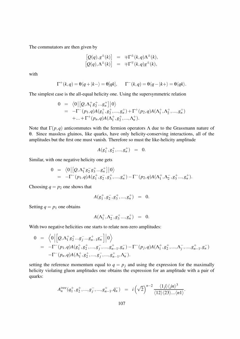
The commutators are then given by
[Q(q),g±(k)
]= ∓Γ±(k,q)Λ±(k),
[Q(q),Λ±(k)
]= ∓Γ∓(k,q)g±(k),
with
Γ+(k,q) = θ〈q+ |k−〉= θ[qk], Γ−(k,q) = θ〈q−|k+〉= θ〈qk〉.
The simplest case is the all-equal helicity one. Using the supersymmetric relation
0 =⟨0∣∣[Q,Λ+
1 g+2 ...g+n
]∣∣0⟩
= −Γ−(p1,q)A(g+1 ,g
+2 , ...,g
+n )+Γ+(p2,q)A(Λ
+1 ,Λ
+2 , ...,g
+n )
+...+Γ+(pn,q)A(Λ+1 ,g
+2 , ...,Λ
+n ).
Note that Γ(p,q) anticommutes with the fermion operators Λ due to the Grassmann nature of
θ. Since massless gluinos, like quarks, have only helicity-conserving interactions, all of the
amplitudes but the first one must vanish. Therefore so must the like-helicity amplitude
A(g+1 ,g+2 , ...,g
+n ) = 0.
Similar, with one negative helicity one gets
0 =⟨0∣∣[Q,Λ+
1 g−2 g+3 ...g+n
]∣∣0⟩
= −Γ−(p1,q)A(g+1 ,g
−2 ,g
+3 , ...,g
+n )−Γ−(p2,q)A(Λ
+1 ,Λ
−2 ,g
+3 ...,g
+n ).
Choosing q = p2 one shows that
A(g+1 ,g−2 ,g
+3 , ...,g
+n ) = 0.
Setting q = p1 one obtains
A(Λ+1 ,Λ
−2 ,g
+3 ...,g
+n ) = 0.
With two negative helicities one starts to relate non-zero amplitudes:
0 =⟨
0
∣∣∣
[
Q,Λ+1 g+2 ...g
−j ...g
+n−1g−n
]∣∣∣0⟩
= −Γ−(p1,q)A(g+1 ,g
+2 , ...,g
−j , ...,g
+n−1,g
−n )−Γ−(p j,q)A(Λ
+1 ,g
+2 , ...,Λ
−j , ...,g
+n−1,g
−n )
−Γ−(pn,q)A(Λ+1 ,g
+2 , ...,g
−j , ...,g
+n−1,Λ
−n ).
setting the reference momentum equal to q = p j and using the expression for the maximally
helicity violating gluon amplitudes one obtains the expression for an amplitude with a pair of
quarks:
Atreen (q+1 ,g
+2 , ...,g
−j , ...,g
+n−1, q
−n ) = i
(√2)n−2 〈1 j〉〈 jn〉3
〈12〉〈23〉...〈n1〉.
107

8.11 Spontaneous breaking of supersymmetry
8.11.1 The mechanism of O’Raifeartaigh
The simplest model consists of three chiral superfields. In this model the superpotential is given
by
W (Φ1,Φ2,Φ3) = λΦ1 +mΦ2Φ3 +gΦ1Φ2Φ2
8.11.2 The mechanism of Fayet and Iliopoulos
Fayet and Iliopoulos considered a model of two chiral superfields Φ1 and Φ2 and a vector super-
field V corresponding to an abelian gauge group. The potential in this model is given by
2κ
(
F1F∗1 +F2F∗
2 +1
2D2
)
.
8.12 The minimal supersymmetric standard model
The supersymmetric part of the minimal supersymmetric standard model (MSSM) reads:
LSUSY =1
8g2Tr WSU(2)WSU(2)
∣∣F+
1
8g′2Tr WU(1)WU(1)
∣∣F+
1
8g2s
Tr WSU(3)WSU(3)
∣∣F+h.c.
+ Qe−2g′V ′T−2gV T−2gsVTs Q
∣∣∣D+ Ue2g′V ′+2gV+2gsVsU
∣∣∣D+ De2g′V ′+2gV+2gsVsD
∣∣∣D
+ Le−2g′V ′T−2gV T
L
∣∣∣D+ Ne2g′V ′+2gV N
∣∣∣D+ Ee2g′V ′+2gV E
∣∣∣D
+ H1e2g′V ′+2gV H1
∣∣∣D+ H2e2g′V ′+2gV H2
∣∣∣D
+[(λdH1QD+λuH2QU +λeH1LE +λνH2LN −µH1H2)|F +h.c.]
Remarks: The Higgs boson is in a chiral superfield and has a spin 1/2 partner, the higgsino.
Anomaly cancellation in the fermion triangle loop requires that there are two Higgs superfields.
The supersymmetric part alone would predict equal masses for all particles in a super-multiplet.
This is not observed. Therefore one adds additional terms to the Lagrange density, which ex-
plicitly break supersymmetry. As these are rather arbitrary, one usually requires that the SUSY-
breaking terms
- generate no quadratic divergences,
- are gauge-invariant,
- conserve R-parity
108

These three conditions define the “soft-breaking-terms”.
Lso f t = −m2q |qL|2 −m2
u |uR|2 −m2d
∣∣dR
∣∣2 −m2
l
∣∣lL∣∣2 −m2
ν |νR|2 −m2e |eR|2
−m21 |H1|2 −m2
2 |H2|2 +1
2
(M1λ′λ′+M2λaλa +M3λa
s λas
)
−εi j
(
λdAdH i1q
jLd
†R +λuAuH i
2qjLu
†R +λeAeH i
1ljLe
†R +λνAνH i
2ljLν†
R −m23H i
1Hj
2 +h.c.)
R-parity: Consider a transformation, which transforms the Grassmann coordinates as
θA → e−iϕ θA → eiϕθA
Furthermore, require that each superfield has a well-defined transformation law under this trans-
formation, like
Φ → eiqΦϕΦ.
qΦ is called the R-charge of the superfield. Writing out the superfield in components
Φ = φ(y)+√
2θψ(y)+θ2F(y),
it is clear that the component fields transform with R-charge
φ : qΦ,
ψ : qΦ +1,
F : qΦ +2.
Assign the R-charge +1 to all quark and lepton superfields, and R-charge 0 to the vector super-
fields and the two Higgs superfields.
R-parity: Restrict eiϕ to ±1.
It then follows with the assignment of the R-charges above, that all standard model-like par-
ticles have R-parity +1, whereas all superpartners have R-parity −1.
Conservation of R-parity implies that at each vertex the product of the R-parities of the involved
particles evaluates to +1. This implies that the supersymmetric particles do always occur in pairs.
Corollar: The lightest supersymmetric particle is stable.
109