INTRODUCTION TO

Polymer Flow Module

C o n t a c t I n f o r m a t i o nVisit the Contact COMSOL page at www.comsol.com/contact to submit general inquiries, contact

Technical Support, or search for an address and phone number. You can also visit the Worldwide

Sales Offices page at www.comsol.com/contact/offices for address and contact information.

If you need to contact Support, an online request form is located at the COMSOL Access page at

www.comsol.com/support/case. Other useful links include:

• Support Center: www.comsol.com/support

• Product Download: www.comsol.com/product-download

• Product Updates: www.comsol.com/support/updates

• COMSOL Blog: www.comsol.com/blogs

• Discussion Forum: www.comsol.com/community

• Events: www.comsol.com/events

• COMSOL Video Gallery: www.comsol.com/video

• Support Knowledge Base: www.comsol.com/support/knowledgebase

Part number. CM025302

I n t r o d u c t i o n t o t h e P o l y m e r F l o w M o d u l e © 1998–2020 COMSOL

Protected by patents listed on www.comsol.com/patents, and U.S. Patents 7,519,518; 7,596,474; 7,623,991; 8,457,932; 9,098,106; 9,146,652; 9,323,503; 9,372,673; 9,454,625; 10,019,544; 10,650,177; and 10,776,541. Patents pending.

This Documentation and the Programs described herein are furnished under the COMSOL Software License Agreement (www.comsol.com/comsol-license-agreement) and may be used or copied only under the terms of the license agreement.

COMSOL, the COMSOL logo, COMSOL Multiphysics, COMSOL Desktop, COMSOL Compiler, COMSOL Server, and LiveLink are either registered trademarks or trademarks of COMSOL AB. All other trademarks are the property of their respective owners, and COMSOL AB and its subsidiaries and products are not affiliated with, endorsed by, sponsored by, or supported by those trademark owners. For a list of such trademark owners, see www.comsol.com/trademarks.

Version: COMSOL 5.6

Contents

The Polymer Flow Module . . . . . . . . . . . . . . . . . . . . . . . . . . . . . . . 5

Newtonian and Non-Newtonian Fluids . . . . . . . . . . . . . . . . . . . . 7

The Polymer Flow Module Physics Interface Guide . . . . . . . . . . 9

Physics Interface Guide by Space Dimension and Study Type . . . 13

Tutorial Example: 2D Non-Newtonian Slot Die Coating. . . . . 16

Model Geometry . . . . . . . . . . . . . . . . . . . . . . . . . . . . . . . . . . . . . . . . 16

Domain Equations and Boundary Conditions . . . . . . . . . . . . . . . . . 17

Results and Discussion . . . . . . . . . . . . . . . . . . . . . . . . . . . . . . . . . . . . 18

References . . . . . . . . . . . . . . . . . . . . . . . . . . . . . . . . . . . . . . . . . . . . . . 19

Tutorial Example: Beads-on-String Structure of Viscoelastic

Filaments . . . . . . . . . . . . . . . . . . . . . . . . . . . . . . . . . . . . . . . . . . . . . 31

Model Geometry . . . . . . . . . . . . . . . . . . . . . . . . . . . . . . . . . . . . . . . . 31

Domain Equations and Boundary Conditions . . . . . . . . . . . . . . . . . 31

Results . . . . . . . . . . . . . . . . . . . . . . . . . . . . . . . . . . . . . . . . . . . . . . . . . 32

Reference. . . . . . . . . . . . . . . . . . . . . . . . . . . . . . . . . . . . . . . . . . . . . . . 33

| 3

4 |

The Polymer Flow Module

Non-Newtonian fluids are found in a great variety of processes in the polymer, food, pharmaceutical, cosmetics, household, and fine chemicals industries. Examples of these fluids are coatings, paints, yogurt, ketchup, colloidal suspensions, aqueous suspensions of drugs, lotions, creams, shampoo, suspensions of peptides and proteins, to mention a few. The Polymer Flow Module is an optional add-on package for COMSOL Multiphysics designed to aid engineers and scientists in simulating flows of non-Newtonian fluids with viscoelastic, thixotropic, shear thickening, or shear thinning properties. Simulations can be used to gain physical insight into the behavior of complex fluids, reduce prototyping costs, and to speed up development. The Polymer Flow Module allows users to quickly and accurately model single-phase flows, multiphase flows, nonisothermal flows, and reacting flows of Newtonian and non-Newtonian fluids.

Figure 1: Coating flow simulation with a power-law fluid. The thickness of the coating layer can be controlled by varying the speed of the lower wall relative to that of the injection slot. Span-wise thickness variations and edge effects may be minimized by optimizing the polymer composition in the coating fluid.

The Polymer Flow Module can solve stationary and time-dependent flows in two-dimensional and three-dimensional domains. Formulations suitable for different types of flow are set up as predefined Fluid Flow interfaces, referred to as physics interfaces. These Fluid Flow interfaces use physical quantities, such as

| 5

velocity and pressure, and physical properties, such as density and viscosity, to define a fluid-flow problem. Different physics interfaces are available to cover a range of flows. Examples include: Laminar Flow, Creeping Flow, Viscoelastic Flow, Heat Transfer, and Transport of Diluted Species. The physics interfaces can be combined with the interfaces in the Mathematics branch (Level Set, Phase Field and Ternary Phase Field), or defined on an Arbitrary Lagrangian Eulerian (ALE) frame to simulate two- and three-phase flows, and rotating flows. The Polymer Flow Module includes a set of predefined multiphysics couplings, including: Nonisothermal Flow; Reacting Flow; Two-Phase Flow, Level Set; Two-Phase Flow, Phase Field; Three-Phase Flow, Phase Field; and Rotating Machinery, Fluid Flow, to facilitate the setup of multiphysics simulations.For each of the physics interfaces, the underlying physical principles are expressed in the form of partial differential equations, together with corresponding initial and boundary conditions. COMSOL’s design emphasizes the physics by providing users with the equations solved by each feature and offering the user full access to the underlying equation system. There is also tremendous flexibility to add user-defined equations and expressions to the system. For example, to model the curing state during a mold injection, a Stabilized Convection Diffusion Equation interface can be added from the Mathematics branch—no scripting or coding is required. When COMSOL compiles the equations the complex couplings generated by these user-defined expressions are automatically included in the equation system. The equations are then solved using the finite element method and a range of industrial-strength solvers. Once a solution is obtained a vast range of postprocessing tools are available to analyze the data, and predefined plots are automatically generated to visualize the results. COMSOL offers the flexibility to evaluate a wide range of physical quantities including predefined quantities such as the pressure, velocity, shear rate, or the vorticity (available through easy-to-use menus), as well as arbitrary user-defined expressions.To set up a fluid flow simulation, the geometry is first defined in the software. Then appropriate materials are selected and suitable physics interfaces together with the appropriate multiphysics couplings are added. Initial conditions and boundary conditions are set up within the physics interfaces. Next, the mesh is defined—in many cases COMSOL’s default mesh, which is produced from physics-dependent defaults, will be appropriate for the problem. A solver is selected, again with defaults appropriate for the relevant physics interfaces, and the problem is solved. Finally the results are visualized. All these steps are accessed from the COMSOL Desktop.

6 |

Newtonian and Non-Newtonian Fluids

A fluid may be characterized according to its response under the action of a shear stress. A Newtonian fluid has a linear relationship between shear stress and shear rate with the line passing through the origin. The constant of proportionality is referred to as the viscosity of the fluid and may depend on temperature, pressure and composition. For a non-Newtonian fluid, the curve for shear stress versus shear rate is nonlinear or does not pass through the origin. If the curve is shifted away from the origin, the fluid has a yield stress. If the curve bends towards the shear-rate axis, the fluid is said to be shear thinning (pseudoplastic), but if it instead bends towards the shear-stress axis, it is said to be shear thickening (dilatant). The relationship may also contain time derivatives of the shear rate to model memory effects (thixotropy), and even parallel viscous and elastic responses. We refer to the latter as viscoelastic non-Newtonian fluids and all others as inelastic non-Newtonian fluids. For the inelastic non-Newtonian models, it is possible to define an apparent viscosity from a generalized Newtonian relationship between the deviatoric stress tensor and the strain-rate tensor.

Figure 2: Conceptual behavior of shear stress versus shear rate for Newtonian, yield-stress, shear-thinning and shear-thickening fluids.

| 7

The apparent viscosity will then be a function of the first invariant of the strain-rate tensor. In simple shear flows, this invariant reduces to the shear rate.The simplest viscoelastic model in the Polymer Flow Module is the Oldroyd-B model which has a constant viscosity and a constant first normal-stress coefficient. This is conceptually visualized as a Hookean spring in series with a dash-pot in Figure 3.

Figure 3: A Hookean spring connected to a dash-pot.

To ensure material-frame indifference, an upper-convected time derivative is used to describe the transport of the additional stress due to the spring and dash-pot. Multiple branches with different relaxation times and viscosities can be added in order to include multi-modal responses. In the Oldroyd-B model, the springs are infinitely extensible, which can lead to unphysical behavior. The other viscoelastic models in the module include nonlinear-spring effects and can also model shear-thinning behavior.When applying a viscoelastic model, it is important to keep in mind that the mathematical formulation may become ill posed at sharp corners. One remedy is to use a fillet operation to smooth the geometry at such points. As always when working with complex fluid flow simulations, it is advisable to start with a simple model, and then switch to a more complicated model if the simple model does not capture the expected flow phenomena. In most industrial applications, inelastic non-Newtonian models produce sufficiently accurate results at a reasonable computational cost.

8 |

The Polymer Flow Module Physics Interface Guide

The physics interfaces in this module are based on the laws for conservation of momentum, mass, and energy in fluids. The different flow models contain different combinations and formulations of the conservation laws that apply to the physics of the flow field. These laws of physics are translated into partial differential equations and are solved together with the specified initial and boundary conditions.A physics interface defines a number of features. These features are used to specify the fluid properties, initial conditions, boundary conditions, and possible constraints. Each feature represents an operation describing a term or condition in the conservation equations. Such a term or condition can be defined on a geometric entity of the component, such as a domain, boundary, edge (for 2D components), or point.Figure 4 shows the Model Builder, including a Laminar Flow interface, and the Settings window for the selected Fluid Properties 1 feature node. The Fluid Properties 1 node adds the marked terms to the component equations in a selected geometry domain. Furthermore, the Fluid Properties 1 feature may link to the Materials feature node to obtain physical properties such as density and constitutive parameters, in this case rubber modeled with a power-law fluid. The fluid properties, defined by the Rubber, Power law material, can be functions of the modeled physical quantities, such as pressure and temperature. In the same way, the Wall 1 node adds the boundary conditions at the walls of the fluid domain.

| 9

Figure 4: The Model Builder including a Laminar Flow interface (left), and the Settings window for Fluid Properties for the selected feature node (right). The Equation section in the Settings window shows the component equations and the terms added by the Fluid Properties 1 node. The added terms are underlined with a dotted line. The arrows also explain the link between the Materials node and the values for the fluid properties.

{

{

10 |

The Polymer Flow Module includes a number of Fluid Flow interfaces for different types of flow. It also includes Chemical Species Transport interfaces for reacting flows in multicomponent solutions, and physics interfaces for heat transfer in solids and in fluids found under the Heat Transfer branch.Figure 5 shows the Polymer Flow Module interfaces as they are displayed when you add a physics interface (see also Physics Interface Guide by Space Dimension and Study Type for further information). A short description of the physics interfaces follows.

Figure 5: The physics interfaces for the Polymer Flow Module as shown in the Model Wizard

SINGLE-PHASE FLOW

The Creeping Flow interface ( ) approximates the Navier-Stokes equations for very low Reynolds numbers. This is often referred to as Stokes flow and is applicable when viscous effects are dominant, such as in very small channels or microfluidics devices.The Laminar Flow interface ( ) is primarily applied to flows at low to intermediate Reynolds numbers. This physics interface solves the Navier-Stokes equations for incompressible, weakly compressible, and compressible flows (up to Mach 0.3). The Laminar Flow interface also allows for simulation of non-Newtonian fluids.

| 11

The Rotating Machinery, Laminar Flow interface ( ) combines the Laminar Flow interface and a Rotating Domain, and is applicable to fluid-flow problems where one or more of the boundaries rotate, for example in mixers and around propellers. The physics interface supports incompressible, weakly compressible and compressible (Mach < 0.3) laminar flows of Newtonian and non-Newtonian fluids.The Viscoelastic Flow interface ( ) is used to simulate incompressible isothermal flow of viscoelastic fluids. It solves the continuity equation, the momentum equation and a constitutive equation that defines the elastic stresses. There are four predefined models for the elastic stresses: Oldroyd-B, FENE-P, Giesekus and LPTT.

MULTIPHASE FLOW

The Two-Phase Flow, Level Set interface ( ), the Two-Phase Flow, Phase Field interface ( ), and the Two Phase Flow, Moving Mesh interface ( ) are used to model two fluids separated by a fluid-fluid interface. The moving interface is tracked in detail using either the level set method, the phase field method, or by a moving mesh, respectively. The level set and phase field methods use a fixed mesh and solve additional equations to track the interface location. The moving mesh method solves the Navier Stokes equations on a moving mesh with boundary conditions to represent the interface. In this case equations must be solved for the mesh deformation. Since a surface in the geometry is used to represent the interface between the two fluids in the Moving Mesh interface, the interface itself cannot break up into multiple disconnected surfaces. This means that the Moving Mesh interface cannot be applied to problems such as droplet formation in inkjet devices (in these applications the level set or phase field interfaces are appropriate). These physics interfaces support incompressible flows, where one or both fluids can be non-Newtonian.The Laminar Three-Phase Flow, Phase Field interface ( ) models laminar flow of three incompressible phases which may be either Newtonian or non-Newtonian. The moving fluid-fluid interfaces between the three phases are tracked in detail using the phase-field method.

NONISOTHERMAL FLOW

The Nonisothermal Flow, Laminar Flow interface ( ) is primarily applied to model flow at low to intermediate Reynolds numbers in situations where the temperature and flow fields have to be coupled. A typical example is natural convection, where thermal buoyancy forces drive the flow. This is a multiphysics interface for which the nonlocal couplings between fluid flow and heat transfer are set up automatically.

12 |

REACTING FLOW

The Laminar Flow interface ( ) under the Reacting Flow branch combines the functionality of the Single-Phase Flow and Transport of Diluted Species interfaces. The physics interface is primarily applied to model flow at low to intermediate Reynolds numbers in situations where the mass transport and flow fields have to be coupled.

Physics Interface Guide by Space Dimension and Study Type

PHYSICS INTERFACE ICON TAG SPACE DIMENSION

AVAILABLE STUDY TYPE

Chemical Species Transport

Transport of Diluted Species1

tds all dimensions stationary; time dependent

Reacting Flow

Laminar Flow, Diluted Species1

— 3D, 2D, 2D axisymmetric

stationary; time dependent

Fluid Flow

Single-Phase Flow

Creeping Flow spf 3D, 2D, 2D axisymmetric

stationary; time dependent

Laminar Flow spf 3D, 2D, 2D axisymmetric

stationary; time dependent

Viscoelastic Flow vef 3D, 2D, 2D axisymmetric

stationary; time dependent

Rotating Machinery, Fluid Flow

Rotating Machinery, Laminar Flow

spf 3D, 2D frozen rotor; time dependent

| 13

Multiphase Flow

Two-Phase Flow, Moving Mesh

Laminar Two-Phase Flow, Moving Mesh

— 3D, 2D, 2D axisymmetric

time dependent

Two-Phase Flow, Level Set

Laminar Two-Phase Flow, Level Set

— 3D, 2D, 2D axisymmetric

time dependent with phase initialization

Two-Phase Flow, Phase Field

Laminar Two-Phase Flow, Phase Field

— 3D, 2D, 2D axisymmetric

time dependent with phase initialization

Three-Phase Flow, Phase Field

Laminar, Three-Phase Flow, Phase Field

— 3D, 2D, 2D axisymmetric

time dependent

Nonisothermal Flow

Laminar Flow(2) — 3D, 2D, 2D axisymmetric

stationary; time dependent; Stationary, one-way NITF; time dependent, one-way NITF

Heat Transfer

Heat Transfer in Fluids1 ht all dimensions stationary; time dependent

Heat Transfer in Solids and Fluids1

ht all dimensions stationary; time dependent

Moving Interface

Level Set ls all dimensions time dependent with phase initialization

PHYSICS INTERFACE ICON TAG SPACE DIMENSION

AVAILABLE STUDY TYPE

14 |

Phase Field pf all dimensions time dependent; time dependent with phase initialization

Ternary Phase Field terpf 3D, 2D, 2D axisymmetric

time dependent

1 This physics interface is included with the core COMSOL package but has added functionality for this module.

2 This physics interface is a predefined multiphysics coupling that automatically adds all the physics interfaces and coupling features required.

PHYSICS INTERFACE ICON TAG SPACE DIMENSION

AVAILABLE STUDY TYPE

| 15

Tutorial Example: 2D Non-Newtonian Slot Die Coating

Achieving uniform coating quality is important in several different industries: from optical coatings, semiconductor and electronics industry, through technologies utilizing thin membranes, to surface treatment of metals. Bad coating quality will compromise the performance of the products, or lead to complete failure in some cases. Several different coating processes exist. This tutorial investigates the performance of a slot-die coating process, a so-called premetered coating method. In this process, the coating fluid is suspended from a thin slot die to a moving substrate. The final coating layer thickness is evaluated from the continuity relationship for a coating liquid. Therefore, the thickness of the liquid layer is determined by the slot gap, the coating fluid inlet velocity and the substrate speed. The final goal of coating processes is to achieve a defect-free film of a desired thickness. However, manufacturing the uniform coating is not a trivial task, various flow instabilities or defects such as bubbles, ribbing, and rivulets are frequently observed in the process. The die geometry, the size of the slot and height above the substrate, together with the non-Newtonian fluid nature of the coating fluid are important to consider.This tutorial demonstrates how to model the fluid flow in a polymer slot die coating process using the Laminar Two-Phase Flow, Phase Field interface and an inelastic non-Newtonian power law model for the polymer fluid.

Model GeometryA typical setup of the slot-die coating process is shown in Figure 6.

Figure 6: Typical geometry for a slot-die coating process with the slot die positioned over a substrate.

This model uses a 2D cross section of the die shown in Figure 6, assuming out-of-plane invariance. See also Slot Die Coating with Channel Defect in the Polymer Flow Module Application Library for a 3D model of slot die coating. The

Die

InletMoving substrate

16 |

inlet for the coating fluid is at the top of the die, as shown in Figure 7, and there are open boundaries at both ends. The bottom boundary is the coating substrate which is moving at the coating velocity.

Figure 7: Model geometry. 2D cross section of a slot die.

The geometrical and material parameters in this model are taken from the Ref. 1.

Domain Equations and Boundary ConditionsThe flow in this model is laminar, so a Laminar Flow interface will be used together with a Phase Field interface to track the interface between the air and the polymer fluid. The coupling of these two interfaces is handled by the Two-Phase Flow, Phase Field multiphysics interface. In this interface, you can select which constitutive relationship to use for each of the fluid phases. The air is specified as a Newtonian fluid, and the coating fluid is a non-Newtonian power law fluid.The inlet fluid velocity is increases smoothly from 0 m/s to 0.1 m/s. Both the upstream and downstream boundaries of the model are specified as open boundaries. The corresponding inlet and outlet boundary conditions must also be set in the Phase Field interface together with the initial values for both fluids to correctly define the position of the initial interface. For the moving substrate, a moving wall boundary condition with a Navier-Slip condition is used.

| 17

Results and DiscussionThe Figure 8 shows the evolution of the coating fluid interface for t = 0.03 s, t = 0.1 s, and t = 0.2 s.

Figure 8: Coating fluid interface at t = 0.03 s, t = 0.1 s and t = 0.2 s. (Top to bottom)

The coating film attains a constant thickness downstream of the die at t = 0.2 s. The film forms upstream and downstream menisci with the upstream and downstream walls of the die. As the substrate speed increases or the inlet velocity decreases, the upstream meniscus is pulled closer to the slot, eventually causing

18 |

defects in the coating film. The evolution of the film thickness and position of the upstream meniscus as a function of time is shown in Figure 9.

Figure 9: Film thickness and upstream meniscus position as a function of time.

By changing the geometry, the inlet velocity and wall velocity, it is easy to explore the sensitivity of the design parameters towards the film thickness and coating velocity for a variety of fluid properties in a fast and efficient manner.

References1. K.L. Bhamidipati, Detection and elimination of defects during manufacture of high-temperature polymer electrolyte membranes, PhD Thesis, Georgia Institute of Technology, 2011.

Model Wizard

1 To start the software, double-click the COMSOL icon on the desktop. When the software opens, you can choose to use the Model Wizard to create a new

| 19

COMSOL model or Blank Model to create one manually. For this tutorial, click the Model Wizard button.If COMSOL is already open, you can start the Model Wizard by selecting New from the File menu and then click Model Wizard .

The Model Wizard guides you through the first steps of setting up a model. The next window lets you select the dimension of the modeling space.

2 In the Model Wizard window, click 2D.3 In the Select Physics tree, select

Fluid Flow>Multiphase Flow>Two-Phase Flow, Phase Field>Laminar Flow.

4 Click Add.5 Click Study.6 In the tree, under Preset Studies for Selected Multiphysics, click

Time Dependent with Phase Initialization .7 Click Done.

Global Definit ions

Load the model parameters from a text file.

Parameters 11 In the Home toolbar click Parameters and select Parameter 1 . Note: On Linux and Mac, the Home toolbar refers to the specific set of controls near the top of the Desktop.

2 Click Load from File.3 Browse to the model’s Application Libraries folder and double-click the file

slot_die_coating_2d_parameters.txt.

Create a step function to use for ramping up the inlet velocity. To improve convergence, define a smoothing transition zone to gently increase the inlet velocity from zero.

Step 11 In the Home toolbar, click Functions and choose Global>Step .2 Locate the Parameters section. In the Location text field, type 0.01.3 Click to expand the Smoothing section. In the Size of transition zone text field,

type 0.02.

20 |

Geometry 1

You can build the slot-die geometry from geometric primitives. Here, instead import the geometry sequence from the model file.Note: The location of the file used in this exercise varies based on your installation. For example, if the installation is on your hard drive, the file path might be similar to C:\Program Files\COMSOL\COMSOL56\Multiphysics\applications\.

1 In the Geometry toolbar choose Insert Sequence .2 Browse to the applications library folder and double-click the file \Polymer_Flow_Module\Tutorials\slot_die_coating_2d.mph.

3 Go to the Home toolbar and click Build All .

Compare the resulting geometry to Figure 7.

Definit ions

Next define integration operators. First define an integration coupling that integrates along the outlet boundary, to calculate the film thickness. Then define a coupling operator that integrates along the upstream die lip. You will use it later for the integration of the volume fraction along the boundary to evaluate the location of the upstream meniscus.

Integration 1 (intop1)1 In the Model Builder window, expand the Component 1 (comp1)>Definitions

node .2 Right-click Definitions and choose Nonlocal Couplings>Integration .3 In the Settings window for Integration, locate the Source Selection section.4 From the Geometric entity level list, choose Boundary.5 Select Boundary 16 only.

Integration 2 (intop2)1 In the Definitions toolbar, click Nonlocal Couplings and choose

Integration.2 In the Settings window for Integration, locate the Source Selection section.3 From the Geometric entity level list, choose Boundary.4 Select Boundary 5 only.

| 21

Materials

Define the materials for the model — air and a coating fluid.

Air1 In the Home toolbar click Add Material .2 Go to the Add Material window. In the

tree under Built-In click Air.3 In the Add Material window, click

Add to Component.4 In the Home toolbar click Add Material

again to close the window.

Coating Fluid1 Right-click Materials and choose Blank Material .2 In the Settings window for Material, type Coating Fluid in the Label text

field.

The physics interface and the chosen fluid model will suggest which material properties should be defined.

Two-Phase Flow, Phase Field

1 In the Model Builder window, under Component 1 (comp1)>Multiphysics click Two-Phase Flow, Phase Field 1 (tpf1) .

2 In the Settings window for Two-Phase Flow, Phase Field, locate the Fluid 1 Properties section.

3 From the Fluid 1 list, choose Air (mat1).4 Locate the Fluid 2 Properties section. From the Fluid 2 list, choose

Coating Fluid (mat2).5 Find the Constitutive relation subsection. From the list, choose

Inelastic non-Newtonian.6 Locate the Surface Tension section. From the Surface tension coefficient list,

choose User defined. In the σ text field, type 0.49.

22 |

Inelastic Non-Newtonian Fluid Parameter Estimation

If you have the Optimization Module in your license, you may use an add-in to calculate the parameters for the power law fluid model based on measurement data in this example. The instructions in the following section show you how to do this. If you do not have access to that license, you may just use the parameters m=7.77 and n=0.86 for the power law coefficients.In the Home toolbar, click Windows and choose Add-in Libraries .Add-in Libraries1 In the Add-in Libraries window, click Refresh.2 In the tree, select

Polymer Flow Module>inelastic_non_newtonian_fluid_parameter_estimation.3 In the tree, select the check box for the node

Polymer Flow Module>inelastic_non_newtonian_fluid_parameter_estimation.4 Click Done.

5 In the Developer toolbar, click Add-ins and choose Inelastic Non-Newtonian Fluid Parameter Estimation>Inelastic Non-Newtonian Fluid Parameter Estimation.

6 In the Model Builder window, under Global Definitions click Inelastic Non-Newtonian Fluid Parameter Estimation 1.

7 In the Settings window for Inelastic Non-Newtonian Fluid Parameter Estimation, click

Load from File.8 Browse to the model’s Application Libraries folder and double-click the file slot_die_coating_2d_viscosity_input.txt.

| 23

9 Click Create to start the parameter estimation.

The power law parameters can now be found in the global parameters table, and thus be used in the material node for the Coating Fluid.

Coating Fluid Parameters

1 In the Model Builder window, under Component 1 (comp1)>Materials click Coating Fluid (mat2).

2 In the Settings window for Material, locate the Material Contents section.

24 |

3 In the table, enter the following settings:

To avoid having the optimization component in the model, use the Clear button in the add-in to clean up the model tree.

Laminar Flow

Now, set up the physics of the problem by defining the domain physics conditions and the boundary conditions.

Wall 21 In the Model Builder window, under Component 1 (comp1) right-click

Laminar Flow (spf) and choose Wall.2 Select Boundary 2 only.3 In the Settings window for Wall, locate the Boundary Condition section.4 From the Wall condition list, choose Navier slip.5 Click to expand the Wall Movement section. Select the Sliding wall check box.6 In the Uw text field, type -U_wall.

Inlet 11 In the Physics toolbar, click Boundaries and choose Inlet.2 Select Boundary 10 only.3 In the Settings window for Inlet, locate the Velocity section.4 In the U0 text field, type step1(t[1/s])*U_in.

Open Boundary 11 In the Physics toolbar, click Boundaries and choose Open Boundary.2 Select Boundaries 1 and 16.

| 25

Phase Field (pf)

The initial interface between the coating fluid and the air is automatically assigned to the boundaries between the two initial value domains. Set up the initial coating fluid domain in the inlet channel.

Initial Values, Fluid 21 In the Model Builder window, under Component 1 (comp1)>Phase Field (pf)

click Initial Values, Fluid 2.2 Select Domain 3 only.

Wetted Wall 11 In the Model Builder window, click Wetted Wall 1.2 In the Settings window for Wetted Wall, locate the Wetted Wall section.3 In the θw text field, type 68.5[deg].

Inlet 11 In the Physics toolbar, click Boundaries and choose Inlet.2 In the Settings window for Inlet, locate the Phase Field Condition section.3 From the list, choose Fluid 2 (φ = 1).4 Select Boundary 10 only.

Outlet 11 In the Physics toolbar, click Boundaries and choose Outlet.2 Select Boundary 16 only.

Wetted Wall 21 In the Physics toolbar, click Boundaries and choose Wetted Wall.2 Select Boundary 2 only.3 In the Settings window for Wetted Wall, locate the Wetted Wall section.4 In the θw text field, type 74[deg].

When working with fluids that have large viscosity and density ratios, switching from the default linear method for the properties averaging can increase the performance. In this model, smoothed Heaviside functions are used to average the fluid properties,

ρ ρ1 ρ2 ρ1–( )HVf,2 0.5–

lρ------------------------ –=

26 |

where is the volume fraction of fluid 2 and is a mixing parameter. A similar expression is used for the dynamic viscosity. To change the averaging method, you must first activate Advanced Physics Options.1 Click the Show More Options button in the Model Builder toolbar.2 In the Show More Options dialog box, in the tree, select the check box for the

node Physics>Advanced Physics Options.3 Click OK.4 In the Model Builder window, under Component 1 (comp1)>Multiphysics

click Two-Phase Flow, Phase Field 1 (tpf1).5 In the Settings window for Two-Phase Flow, Phase Field, click to expand the

Advanced Settings section.6 From the Density averaging list, choose Heaviside function.7 In the lρ text field, type 0.9.8 From the Viscosity averaging list, choose Heaviside function.9 In the lμ text field, type 0.9.

The mixing parameter can be decreased to sharpen the interface, but that will increase the computation time for this example.

Study 1

If you want to inspect the progress of the fluids during the simulation, you can enable the plot while solving option in the Step 2: Time Dependent node. By calculating the initial values first, the solver sequence and default plots will be generated. In the following section you generate the default plot groups and use one of them for plotting the volume fraction while solving. Note that plot while solving in general will affect the computation time slightly since the plot needs to be updated in each time step.1 In the Study toolbar, click Get Initial Value.2 In the Model Builder window, under Study 1 click Step 2: Time Dependent.3 In the Settings window for Time Dependent, click to expand the

Results While Solving section.4 Select the Plot check box.5 From the Plot group list, choose Volume Fraction of Fluid 1 (pf).6 From the Update at list, choose Time steps taken by solver.7 Locate the Study Settings section. In the Output times text field, type range(0,0.01,0.25).

Vf,2 lρ

| 27

8 In the Study toolbar, click Compute.

Results

Examine the default plot at t = 0.03, 0.1, and 0.2 (s)

Volume Fraction of Fluid 1 (pf)1 In the Model Builder window, under Results click

Volume Fraction of Fluid 1 (pf).2 In the Settings window for 2D Plot Group, locate the Data section.3 From the Time (s) list, choose 0.03.4 In the Volume Fraction of Fluid 1 (pf) toolbar, click Plot.5 From the Time (s) list, choose 0.1.6 In the Volume Fraction of Fluid 1 (pf) toolbar, click Plot.7 From the Time (s) list, choose 0.2.8 In the Volume Fraction of Fluid 1 (pf) toolbar, click Plot.

Coating fluid interface at t = 0.03 s, t = 0.1 s and t = 0.2 s. (Top to bottom).

28 |

Proceed to reproduce the plot of the film thickness and the upstream meniscus position.

Film Thickness and Upstream Meniscus Position1 In the Home toolbar, click Add Plot Group and choose 1D Plot Group.2 In the Settings window for 1D Plot Group, type Film Thickness and Upstream

Meniscus Position in the Label text field.3 Locate the Legend section. From the Position list, choose Upper left.

Global 11 Right-click Film Thickness and Upstream Meniscus Position and choose

Global.2 In the Settings window for Global, locate the y-Axis Data section.3 In the table, enter the following settings:

A high value (0.95) for the limit of the coating fluid volume fraction is used to safeguard against air entrainment into the coating layer.

4 In the Film Thickness and Upstream Meniscus Position toolbar, click Plot.

| 29

Film thickness and upstream meniscus position as a function of time.

30 |

Tutorial Example: Beads-on-String Structure of Viscoelastic Filaments

In this example, the thinning of a viscoelastic filament under the action of surface tension is studied. The evolution of the filament radius depends on the relative magnitude of capillary, viscous, and elastic stresses. The interplay of capillary and elastic stresses leads to the formation of very thin and stable filaments between drops, a so called beads-on-a-string structure.

Model GeometryThis example studies the evolution of a long, initially unstretched axisymmetric filament of an Oldroyd-B fluid. The fluid filament is modeled as a liquid cylinder with a small perturbation of the initial radius of the cylinder, R0 (Figure 10, t = 0). The initial radius of the column is given by

where z is the z-coordinate and ε is the perturbation magnitude.

Domain Equations and Boundary ConditionsThe Oldroyd-B fluid used in this example is viscoelastic and you should therefore use the Viscoelastic Flow interface. An arbitrary Lagrangian-Eulerian (ALE) method is used to handle the dynamics of the deforming geometry and moving boundaries. The Navier–Stokes equations for fluid flow and the evolution

r z 0,( ) R0 1 ε z2R0----------cos+

, 0 zR0------- 8π≤ ≤=

| 31

equations for the elastic stress tensor components are formulated in the coordinates of the moving frame.A Free Surface feature is applied at the interface between the polymer fluid and the air. This feature sets up the surface-tension force and specifies the normal velocity of the free surface. The outside air pressure is assumed to be constant, and the tangential stress on the free surface is neglected. A Periodic Flow Condition feature is used at the top and bottom boundaries to mimic the effect of an infinitely long filament.The problem is made dimensionless by the initial radius of the cylinder, R0, the surface tension coefficient σ, the fluid density ρ, and the total viscosity, μ0, of the polymer. The dynamics of the of the filament thinning is governed by two dimensionless parameters: the Deborah number (the dimensionless relaxation time of the polymer solution) and the Ohnesorge number (the ratio between the inertia-capillary and viscous-capillary time scales). The relative importance of viscous stresses from the solvent is characterized by the solvent viscosity ratio, β.

ResultsFigure 10 shows the evolution of the filament at different times for the following set of the dimensionless parameters: β = 0.25, Oh = 3.16, and De = 94.9.

Figure 10: Filament profiles at 5 different dimensionless times: 0, 20, 30, 100, and 300

The transformation of the filament shape can be divided into two regimes with distinct time scales. First, for times smaller than the polymer relaxation time, the

32 |

beads-on-string structure develops. This is followed by an exponential thinning of the threads. The fluid is expelled from the threads to the connected beads leading to almost spherical drops. The numerical results show that both transient regimes compare well with the literature (Ref. 1).

Reference1. C. Clasen, J. Eggers, M. A. Fontelo, J. Li, G. McKinley, The beads-on-string structure of viscoelastic threads, J. Fluid Mech.,vol.556, pp.283-308, 2006.

The following instructions show how to set up the model, solve it, and plot the results.

Model Wizard

Note: These instructions are for the user interface on Windows but apply, with minor differences, also to Linux and Mac.

1 To start the software, double-click the COMSOL icon on the desktop. When the software opens, you can choose to use the Model Wizard to create a new COMSOL model or Blank Model to create one manually. For this tutorial, click the Model Wizard button.If COMSOL is already open, you can start the Model Wizard by selecting New from the File menu and then click Model Wizard .

The Model Wizard guides you through the first steps of setting up a model. The next window lets you select the dimension of the modeling space.

2 In the Select Space Dimension window, click the 2D Axisymmetric button .3 In the Select Physics tree, select

Fluid Flow>Single-Phase Flow>Viscoelastic Flow (vef) .4 Click Add and then the Study button .5 In the tree, under General Studies, click Time Dependent .6 Click the Done button .

Root

The equations are formulated in dimensionless form. Proceed to change the Unit System for the model.

| 33

1 In the Model Builder window, click the root node .2 In the root node’s Settings window, locate the Unit System section.3 From the Unit system list, choose None.

Global Definit ions

Parameters 11 In the Model Builder window, under Global Definitions click Parameters 1.2 In the Settings window for Parameters, locate the Parameters section.3 Enter the values of the perturbation magnitude and the dimensionless

parameters:

Geometry 1

Create the geometry by using a parametric curve and a polygon.

Parametric Curve 1 (pc1)1 In the Geometry toolbar, click More Primitives and choose

Parametric Curve.2 In the Settings window for Parametric Curve, locate the Parameter section.3 In the Maximum text field, type 8*pi.4 Locate the Expressions section. In the r text field, type 1+epsilon*cos(s/2).5 In the z text field, type s.6 Click Build Selected.

Polygon 1 (pol1)1 In the Geometry toolbar, click Polygon.

NAME EXPRESSION VALUE DESCRIPTION

epsilon 0.05 0.05 Radius perturbation

beta 0.25 0.25 Solvent viscosity ratio

Oh 3.16 3.16 Ohnesorge number

De 94.9 94.9 Deborah number

mus beta*Oh 0.79 Solvent viscosity

mup (1-beta)*Oh 2.37 Elastic viscosity

34 |

2 In the Settings window for Polygon, locate the Object Type section.

3 From the Type list, choose Open curve.4 Locate the Coordinates section. In the table, enter the following

settings:

5 Click Build All Objects.6 Convert to Solid 1 (csol1)7 In the Geometry toolbar, click Conversions and choose

Convert to Solid.8 Click in the Graphics window and then press Ctrl+A to select both

objects.9 In the Settings window for Convert to Solid, click

Build All Objects.

Definit ions

Deforming Domain 11 In the Definitions toolbar, click

Moving Mesh and choose Deforming Domain.

2 Select Domain 1 only.3 In the Settings window for

Deforming Domain, locate the Smoothing section.

4 From the Mesh smoothing type list, choose Hyperelastic.

R Z

1+epsilon 0

0 0

0 8*pi

1+epsilon 8*pi

| 35

Viscoelastic Flow (vef)

1 In the Model Builder window, under Component 1 (comp1) click Viscoelastic Flow (vef).

2 In the Settings window for Viscoelastic Flow, click to expand the Discretization section.

3 From the Discretization of fluids list, choose P1+P1.

Note: Several default nodes are added automatically to the model tree. The ‘D’ in the upper left corner of the node indicates that these are default nodes.

Fluid Properties 11 In the Model Builder window, under

Component 1 (comp1)>Viscoelastic Flow (vef) click Fluid Properties 1.2 In the Settings window for Fluid Properties, locate the Fluid Properties section.3 From the r list, choose User defined. In the associated text field, type 1.4 For the Viscoelastic interface, Viscoelastic, Newtonian, and Inelastic

non-Newtonian constitutive relations are available. By default, the viscoelastic Oldroyd-B model is selected.

5 Choose User defined from the ms list. In the associated text field, type mus.6 In the table, enter values for elastic viscosity and relaxation time:

BRANCH VISCOSITY RELAXATION TIME

1 mup De

36 |

Free Surface 1The viscosity of the air is negligible compared to that of the viscoelastic fluid. Only the air pressure is accounted for on the exterior side of the free surface.1 In the Physics toolbar, click Boundaries and choose Free Surface.2 Select Boundary 4 only.3 In the Settings window for Free Surface, locate the Surface Tension section.4 From the Surface tension coefficient list, choose User defined. In the s text

field, type 1.

Contact Angle 11 In the Model Builder window, expand the Free Surface 1 node, then click

Contact Angle 1.2 In the Settings window for Contact Angle, locate the Normal Wall Velocity

section.3 Select the Constrain wall-normal velocity check box.

Periodic Flow Condition 11 In the Physics toolbar, click Boundaries and choose

Periodic Flow Condition.2 Select Boundaries 2 and 3 only.

Additionally, mesh boundary conditions are needed on all exterior boundaries (except for the Free Surface, which automatically includes the necessary mesh constraint).

Definit ions

Symmetry/Roller 11 In the Definitions toolbar, click Moving Mesh and choose Symmetry/

Roller.2 In the Settings window for Symmetry/Roller, locate the Boundary Selection

section.

| 37

3 Select Boundaries 1, 2, and 3 on (top, bottom and symmetry boundaries).

Mesh 1

Free Triangular 1In the Mesh toolbar, click Free Triangular.

Size4 In the Model Builder window, click Size.5 In the Settings window for Size, locate the

Element Size section.6 From the Calibrate for list, choose

Fluid dynamics.7 From the Predefined list, choose

Extremely coarse.8 Click to expand the Element Size Parameters

section. In the Minimum element size text field, type 0.001.

9 In the Resolution of narrow regions text field, type 8.

10Click Build All

38 |

Study 1

Step 1: Time Dependent1 In the Model Builder window, expand the Study 1>Step 1: Time Dependent

node, then click Step 1: Time Dependent.2 In the Settings window for Time Dependent, locate the Study Settings section.

In the Output times text field, type range(0,5,300).3 From the Tolerance list, choose User controlled.4 In the Relative tolerance text field, type 0.005.5 Click to expand the Study Extensions section. Select the Automatic remeshing

check box.

Before solving the problem, prepare a plot of the velocity. The plot will be shown and updated during the computations. In the Study toolbar, click

Get Initial Value. Default plots for the velocity and pressure are generated automatically.

| 39

Results

Mirror 2D 11 In the Results toolbar, click More Datasets and choose Mirror 2D.

2 In the Settings window for Mirror 2D, locate the Data section.3 From the Dataset list, choose Study 1/Remeshed Solution 1 (sol2).4 Click Plot.

Velocity (vef)1 In the Model Builder window, expand the Results>Velocity (vef) node, then

click Velocity (vef).2 In the Settings window for 2D Plot Group, locate the Data section.3 From the Dataset list, choose Mirror 2D 1.

Study 1

Step 1: Time Dependent1 In the Model Builder window, under Study 1 click Step 1: Time Dependent.2 In the Settings window for Time Dependent, click to expand the

Results While Solving section.3 Select the Plot check box.4 From the Update at list, choose Time steps taken by solver.

40 |

Getting the initial values for the step also creates the solver suggestions based on the existing physics.

Solver ConfigurationsIn the Model Builder window, expand the Study 1>Solver Configurations node.

Solution 1 (sol1)1 In the Model Builder window, expand the

Study 1>Solver Configurations>Solution 1 (sol1) node, then click Time-Dependent Solver 1.

2 In the Settings window for Time-Dependent Solver, click to expand the Time Stepping section.

3 From the Method list, choose Generalized alpha.1 From the Maximum step constraint list, choose Expression.2 In the Maximum step text field, type comp1.vef.dt_CFL.3 In the Model Builder window, expand the

Study 1>Solver Configurations>Solution 1 (sol1)>Time-Dependent Solver 1 node, then click Automatic Remeshing.

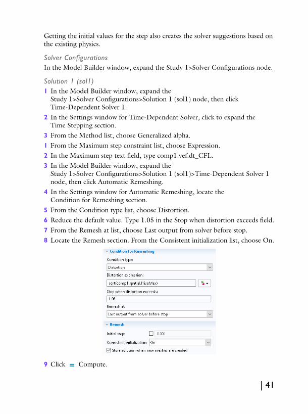
4 In the Settings window for Automatic Remeshing, locate the Condition for Remeshing section.

5 From the Condition type list, choose Distortion.6 Reduce the default value. Type 1.05 in the Stop when distortion exceeds field.7 From the Remesh at list, choose Last output from solver before stop.8 Locate the Remesh section. From the Consistent initialization list, choose On.

9 Click Compute.

| 41

Results

After the computation the velocity plot for the final time will be shown

Continue with a visualization of the filament shape at selected times (Figure 10).

Shape1 In the Model Builder window, right-click Velocity (vef) and choose Duplicate.2 In the Settings window for 2D Plot Group, type Shape in the Label text field.

Surface1 In the Model Builder window, expand the Shape node, then click Surface.2 In the Settings window for Surface, locate the Expression section.3 In the Expression text field, type 1.4 Locate the Coloring and Style section. From the Coloring list, choose Uniform.5 From the Color list, choose Black. The plot shows the shape at the last time

step, t=300.6 In the Settings window for Surface, locate the Data section.

7 From the Time (s) list, choose 0, 20, 30, 100 to plot the shape evolution at different times.

Now, plot the minimum filament radius.

42 |

Line Minimum 11 In the Results toolbar, click

Numerical and then More Derived Values and choose Minimum>Line Minimum.

2 Select the Boundary 4 only.3 In the Settings window for

Line Minimum, locate the Expressions section, enter log10(r).

4 Locate the Data section. From the Dataset list, choose Study 1/Remeshed Solution 1 (sol2).

5 Click Evaluate.

TableThe result appears in the Table window at the bottom of the COMSOL Desktop. Click Table Graph in the window toolbar.

Results

Minimum Radius1 In the Model Builder window, under Results click 1D Plot Group 5.2 In the Settings window for 1D Plot Group, type Minimum Radius in the Label

text field.3 Click to expand the Title section. Locate the Plot Settings section. Select the

x-axis label check box.4 Select the y-axis label check box.5 In the x-axis label text field, type t.6 In the Minimum Radius toolbar, click Plot .

| 43

The plot shows the minimum filament radius as a function of time. After a rapid formation of the beads-on-string structure, the figure shows the slow thinning of the threads. The rate of thinning is determined by the balance of surface tension and the elastic forces. Under the assumption of a spatially constant and slender profile, an asymptotic solution to the problem can be derived. Plot the asymptotic solution using the following steps.

Grid 1D 11 In the Results toolbar, click More Datasets and choose Grid>Grid 1D.2 In the Settings window for Grid 1D, locate the Parameter Bounds section.3 In the Minimum text field, type 50, in the Maximum text field, type 300.

Minimum RadiusIn the Model Builder window, click Minimum Radius.

Function 11 In the Minimum Radius

toolbar, click More Plots and choose Function.

2 In the Settings window for Function, locate the y-Axis Data section.

3 In the Expression text field, enter the asymptotic expression -1/(3*De*log(10))*x-0.3.

4 Locate the x-Axis Data section. In the Expression text field, type x.5 In the Lower bound text field, type 150.6 In the Upper bound text field, type 250.7 Locate the Data section. From the Dataset list, choose Grid 1D 1.8 Click to expand the Coloring and Style section. Find the Line style subsection.

From the Line list, choose Dashed.9 In the Width text field, type 2.10From the Color list, choose Black.11Click to expand the Legends section. Select the Show legends check box.12From the Legends list, choose Manual.13Type slope=-1/(3*De*log(10))in the table.

44 |

14In the Minimum Radius toolbar, click Plot .

The figure shows that the evolution of the minimum radius agrees well with the asymptotic prediction for large times.

| 45

46 |