introduction to the foundations of quantum optimal control
TRANSCRIPT
Introduction to the Pontryagin Maximum
Principle for Quantum Optimal Control
U. Boscain∗, M. Sigalotti†, D. Sugny‡
September 16, 2021
Abstract
Optimal Control Theory is a powerful mathematical tool, which hasknown a rapid development since the 1950s, mainly for engineering appli-cations. More recently, it has become a widely used method to improveprocess performance in quantum technologies by means of highly efficientcontrol of quantum dynamics. This tutorial aims at providing an intro-duction to key concepts of optimal control theory which is accessible tophysicists and engineers working in quantum control or in related fields.The different mathematical results are introduced intuitively, before be-ing rigorously stated. This tutorial describes modern aspects of optimalcontrol theory, with a particular focus on the Pontryagin Maximum Prin-ciple, which is the main tool for determining open-loop control laws with-out experimental feedback. The different steps to solve an optimal controlproblem are discussed, before moving on to more advanced topics such asthe existence of optimal solutions or the definition of the different typesof extremals, namely normal, abnormal, and singular. The tutorial coversvarious quantum control issues and describes their mathematical formula-tion suitable for optimal control. The connection between the PontryaginMaximum Principle and gradient-based optimization algorithms used forhigh-dimensional quantum systems is described. The optimal solution ofdifferent low-dimensional quantum systems is presented in detail, illus-trating how the mathematical tools are applied in a practical way.
Contents
1 Introduction 2
2 Introduction to the optimal control concepts: The case of atwo-level quantum system 5
3 Formulation of the control problem 7
∗Laboratoire Jacques-Louis Lions, CNRS, Inria, Sorbonne Universite, Universite de Paris,France, [email protected]
†Laboratoire Jacques-Louis Lions, CNRS, Inria, Sorbonne Universite, Universite de Paris,France, [email protected]
‡Laboratoire Interdisciplinaire Carnot de Bourgogne (ICB), UMR 6303 CNRS-UniversiteBourgogne-Franche Comte, 9 Av. A. Savary, BP 47 870, F-21078 Dijon Cedex, France,[email protected]
1
arX
iv:2
010.
0936
8v2
[qu
ant-
ph]
15
Sep
2021
4 The different steps to solve an optimal control problem 11
5 Existence of solutions for Optimal Control Problem: the Filip-pov test 12
6 First-order conditions 156.1 Why Lagrange multipliers appear in constrained optimization
problems . . . . . . . . . . . . . . . . . . . . . . . . . . . . . . . . 156.2 Statement of the Pontryagin Maximum Principle . . . . . . . . . 176.3 Use of the PMP . . . . . . . . . . . . . . . . . . . . . . . . . . . . 20
7 Gradient-based optimization algorithm 227.1 The Weak Pontryagin Maximum Principle . . . . . . . . . . . . . 227.2 Gradient-based optimization algorithm . . . . . . . . . . . . . . . 24
8 Example 1: A three-level quantum system with complex con-trols 258.1 Formulation of the quantum control problem . . . . . . . . . . . 258.2 Existence . . . . . . . . . . . . . . . . . . . . . . . . . . . . . . . 278.3 Application of the PMP . . . . . . . . . . . . . . . . . . . . . . . 29
9 Example 2: A minimum time two-level quantum system witha real control 349.1 Formulation of the control problem . . . . . . . . . . . . . . . . . 349.2 Application of the PMP . . . . . . . . . . . . . . . . . . . . . . . 36
10 Applications of quantum optimal control theory 41
11 Conclusion 42
12 List of notations 43
A Test of controllability 44
B Filippov’s theorem 44
1 Introduction
Quantum technology aims at developing practical applications based on proper-ties of quantum mechanics [1]. This objective requires precise manipulation ofquantum objects by means of external electromagnetic fields. Quantum controlencompasses a set of techniques to find the time evolution of control parameterswhich perform specific tasks in quantum physics [2, 3, 4, 5, 6, 7, 8, 9, 10, 11, 12,13, 14, 15, 16, 17, 18, 19]. In recent years, it has naturally become a key toolin the emergent field of quantum technologies [1, 20, 2], with applications rang-ing from quantum computing [2, 21, 22] to quantum sensing [23] and quantumsimulation [24, 25].
In the majority of quantum control protocols, the control law is computedin an open-loop configuration without experimental feedback. In this context,a powerful tool is Optimal Control Theory (OCT) [2] which allows a given pro-cess to be carried out, while minimizing a cost (e.g., the control time). This
2

approach has key advantages. Its flexibility makes it possible to adapt to exper-imental constraints or limitations and its optimal character leads to the physicallimits of the driven dynamics. OCT can be viewed as a generalization of theclassical calculus of variations for problems with dynamical constraints [26]. Itsmodern version was born with the Pontryagin maximum principle (PMP) inthe late 1950s [27]. Since the pioneering study of Pontryagin and co-workers,OCT has undergone rapid development and is nowadays a recognized field ofmathematical research. Recent tools from differential geometry have been ap-plied to control theory, making these methods very effective in dealing withproblems of growing complexity. Many reference textbooks have been pub-lished on the subject both on mathematical results and engineering applica-tions [28, 29, 30, 31, 26, 32, 33, 34, 36, 35]. Originally inspired by problems ofspace dynamics, OCT was then applied in a wide spectrum of applications suchas robotics or economics. OCT was first used for quantum processes [37, 38]in the context of physical chemistry, the goals being to steer chemical reac-tions [39, 40, 4, 41, 42] or to control spin dynamics in Nuclear Magnetic Res-onance [43, 44, 45, 46]. A lot of results have recently been established forquantum technologies, as for example the minimum duration to generate high-fidelity quantum gates [2].Two types of approach based on the PMP have been used to solve optimal con-trol problems in low- and high-dimensional systems, respectively. In the firstsituation called geometric optimal control theory, the equations for optimalityare solved by using geometric and analytical tools. The results can be deter-mined analytically or at least with a very high numerical precision. The PMPallows to deduce the structure of the optimal solutions and, in some cases, aproof of their global optimality can be established. In this context, a series oflow-dimensional quantum control problems has been rigorously solved in recentyears for both closed [47, 48, 49, 50, 51, 52, 53, 54, 55, 56] and open quantum sys-tems [57, 58, 59, 60, 61, 62, 63, 64]. Specific numerical optimization algorithmshave been developed and applied to design control fields in larger quantum sys-tems [45, 65, 25, 66, 67]. Due to the complexity of control landscape, only localoptimal solutions are found with this numerical optimal control approach.
However, despite the recent success of quantum optimal control theory, thesituation is still not completely satisfactory. The difficulty of the concepts usedin this field does not allow a non-expert to understand and apply easily thesetechniques. The mathematical textbooks use a specialized and sophisticatedlanguage, which makes these works difficult to access. Very few basic papersfor physicists are available in the literature, while having a minimum grasp ofthese tools will be an important skill in the future of quantum technologies. Thepurpose of this tutorial is to provide an introduction to the core mathematicalconcepts and tools of OCT in a rigorous but understandable way by physicistsand engineers working in quantum control and in related fields. A deep analogycan be carried out between OCT and finding the minima of a real functionof several variables. This parallel is used throughout the text to qualitativelydescribe the key aspects of the PMP. The tutorial is based on an advanced coursefor PhD students in physics taught at Saarland University in Spring of 2019.It assumes a basic knowledge of standard topics in quantum physics, but alsoof mathematical techniques such as linear algebra or differential calculus andgeometry. Finally, we hope that this paper will give the reader the prerequisitesto access a more specialized literature and to apply optimal control techniques
3

to their own control problems.
Structure of the paper
A tutorial about optimal control is a difficult task because a large number ofmathematical results have been obtained and many techniques have been devel-oped over the years for specific applications. Among others, we can distinguishthe following problem classes: finite or infinite-dimensional systems, open orclosed-loop control, linear or nonlinear dynamical systems, geometric or numer-ical optimal control, PMP or Hamilton–Jacobi–Bellmann (HJB) approach. . .We briefly recall that the HJB method which is the result of the dynamic pro-gramming theory leads to necessary and sufficient conditions for optimality inwhich the optimal cost is solution of a nonlinear partial differential equation [26].Unfortunately, this equation is generally very difficult to solve numerically.
This means making choices about which topics to include in this paper. Wehave deliberately selected specific aspects of OCT that are treated rigorously,while others are only briefly mentioned. The choice fell on basic mathematicalconcepts which are the most useful in quantum control. We limit our focus onthe optimal control of open-loop finite-dimensional system by using the PMP.In particular, we consider only analytical and geometric techniques to solve low-dimensional control problems. To ensure overall consistency and limit the lengthof the paper, we do not discuss in depth numerical optimization methods and theinfinite-dimensional case [68, 69], which are also key issues in quantum control.In order to connect this tutorial with the current applications of optimal controlto high-dimensional quantum system, we describe the link between the PMP andthe most current implementation of the gradient-based optimization algorithm(the GRAPE algorithm [45]). Finally, we stress that a precise knowledge of thePMP is an essential skill for numerical optimization, and that the scope of thematerial of this paper is much broader than the examples presented.
The paper is built on three reading levels. A first level corresponds to themain text and explains the main concepts necessary to describe and apply thetheory of optimal control. Some key ideas in optimal control are first introducedqualitatively for a simple quantum system in Sec. 2. In addition to the two ex-amples solved in Sec. 8 and 9, the different notions are described rigorously andthen systematically illustrated by examples. This establishes a direct link be-tween the mathematical concept and its practical application. A second readinglevel is given by footnotes, which recall a mathematical definition or correspondto a more specific comment which can be skipped on a first reading. A finalreading level is available in the appendices. These different paragraphs explainin detail the mathematical origin of the theorems used for the controllabilityand the existence problem and some standard counter-examples or specificitiesthe reader should have in mind. We point out that these sections are not mathe-matical proofs of theorems, but rather a description of the formalism introducedin a language accessible to a physicist. In order to facilitate the reading of thepaper, a list of the main notations used is given in Sec. 12 with the place of thetext where they are first introduced.
Although the paper is thought for a physics audience and the mathematicaldetails are kept as simple as possible, our objective is to stick to rigorous state-ments and claims, since this aspect becomes crucial while implementing optimalcontrol ideas in numerical simulations or in experiments.
4

The paper is organized as follows. We first introduce the main ideas usedin optimal control in the case of a simple quantum system in Sec. 2. We thenshow how to formulate an optimal control problem from a mathematical pointof view in Sec. 3. Closed and open quantum systems illustrate this discussion.The different steps to solve such a problem are presented in Sec. 4 by using theanalogy with finding a minimum of a function of several variables. The tutorialcontinues with a point which is crucial, but often overlooked in quantum controlstudies, namely the existence of optimal solutions. We present in Sec. 5 someresults based on the Filippov test, which is one of the most important techniquesto address this question. The first-order conditions are described in Sec. 6, witha specific attention on the different types of extremals and on the statement ofthe PMP. The connection between the PMP and gradient-based optimizationalgorithms is described in Sec. 7. Sections 8 and 9 are dedicated to the presen-tation of two examples in three and two-level quantum systems, respectively.Recent advances in the application of OCT to quantum technologies are brieflydescribed in Sec. 10, where we mention some of the current directions that arebeing followed for the development of these techniques. A conclusion is given inSec. 11. Mathematical details about the controllability and existence problemsare postponed, respectively, to Appendices A and B.
2 Introduction to the optimal control concepts:The case of a two-level quantum system
In quantum control, a general problem is to prepare a given quantum state bymeans of a specific time-dependent electromagnetic pulse. This leads to somequestions such as which states can be achieved or which shape of control isrequired to realize this objective. These aspects, which are addressed rigorouslyin the rest of the tutorial, are first introduced qualitatively in this section.
To this aim, we consider the control driving a two-level quantum system fromthe ground to the excited state. The system is described by a wave functionψ(t) whose dynamics are governed by the Schrodinger equation
iψ =
(E0 Ω(t)
Ω∗(t) E1
)ψ,
where units such that ~ = 1 have been chosen. The parameters E0 and E1
denote respectively the energies of the ground and excited states, while Ω(t)corresponds (up to a multiplicative factor) to a complex external field whosereal and imaginary parts are, e.g., the components of two orthogonal linearlypolarized laser fields. We consider resonant fields for which the carrier frequencyω of the laser is equal to the energy difference E1 − E0, namely,
Ω(t) = u(t)ei(E1−E0)t,
where the amplitude u(t) represents the control and is assumed to be real. Wenow apply a time-dependent change of variables corresponding to the choice of arotating frame. The time evolution of ψ = Υ−1ψ, with Υ = diag(e−iE0t, e−iE1t),satisfies the differential equation
i˙ψ =
(0 u(t)u(t) 0
)ψ.
5
We denote by c1 = x1 + iy1 and c2 = x2 + iy2 the two complex coordinatesof ψ in a basis of the Hilbert space C2 where the indices 1 and 2 correspondrespectively to the ground and excited states. Since ψ is a state of norm 1 andΥ a unitary operator, we deduce that x2
1 + y21 + x2
2 + y22 = 1. Starting from
the state x1 = 1, the goal of the control is to bring the system to a target forwhich x2
2 + y22 = 1. The Schrodinger equation is equivalent to the following set
of equations for the coefficients xk and yk:x1 = uy2
y1 = −ux2
x2 = uy1
y2 = −ux1.
Since u is a real control, we immediately see that the first and the last equationsare coupled to each other and decoupled from the two others. In other words, theinitial state of the dynamics is only connected to states for which y1 = x2 = 0,i.e., such that x2
1 + y22 = 1. The system thus evolves on a circle. For our control
objective, the only interesting states correspond therefore to y2 = ±1. It is alsostraightforward to verify that such target states can be reached at least with aconstant control u. In control theory, this formulation of the control problemand the analysis of the reachable set from the initial state constitute a basicprerequisite before deriving a specific control procedure. This step is detailedin Sec. 3.
We now explore the optimal control of this system. We first use the circulargeometry of the dynamics to simplify the corresponding equations. We introducethe angle θ such that x1 = cos θ and y2 = sin θ, with θ(0) = 1. We arrive at
θ = −u(t),
where the target state is here defined as θfi = ±π2 . By symmetry, we can fixwithout loss of generality θfi = −π2 . Many control solutions u exist to reach thisstate and a specific protocol can be selected by minimizing at the same time afunctional of the state of the system and of the control, called a cost. Here, anexample is given by the control time. To summarize in this example, the goal ofthe optimal control procedure is then to find the control u steering the systemto the target state in minimum time. Consider first constant controls u(t) = u0
with u0 ∈ R. The duration of the process is thus T = π2u0
. This solution revealsa key problem in optimal control which corresponds to the existence of a mini-mum. In this example, arbitrarily fast controls can be achieved by consideringlarger and larger amplitudes u0 and an optimal trajectory minimizing the trans-fer time does not exist. The analysis of the existence of optimal solutions whichis a building block of any rigorous description of an optimal control problem isdiscussed in Sec. 5. It can be shown with the results presented in Sec. 5 that anoptimal solution exists if the set of available controls is restricted to a boundedinterval, e.g., u(t) ∈ [−um, um] where um is the maximum amplitude. In thiscase, the optimal pulse is the control of maximum amplitude, the minimum timebeing equal to π/2um.
In order to illustrate the method of solving an optimal control problem, weconsider the same transfer but in a fixed time T , the goal being to minimize
the energy associated with the control, i.e., the term∫ T
0u(t)2
2 dt. There is no
6

additional constraint on the control and we have u(t) ∈ R. The target state
is reached if∫ T
0u(t)dt = π
2 . Introducing the Lagrange multiplier λ ∈ R, thisconstrained optimization problem can be transformed into the minimization ofthe functional
J =
∫ T
0
(u(t)2
2+ λu(t)
)dt− λπ
2.
If we denote by H the function H = −u2
2 − λu, the Euler-Lagrange principle
leads to ∂H∂u = 0, i.e., u(t) = −λ. Using the constraint on the dynamics, we
finally arrive at the optimal control u(t) = π2T .
In this simple example, the optimal solution can be derived without thecomplete machinery of the Pontryagin Maximum Principle presented below.However, in the example we have introduced the main tools used in the PMP,such as the Lagrange multiplier, the Pontryagin Hamiltonian H, and the maxi-mization condition ∂H
∂u = 0. A few comments are in order here. The dynamicalconstraint is quite simple since the dimension of the state space is the sameas the number of controls, the dynamics can be exactly integrated and the set
of controls satisfying the constraint∫ T
0u(t)dt = π
2 is regular. This is not thecase for a general nonlinear control system for which (1) the Lagrange multi-plier (which usually is not constant but a function of time) is not easily found,(2) abnormal Lagrange multipliers appear if the set of controls satisfying theconstraint is not regular. We observe that H can be rewritten as
H = λθ − u2
2,
which corresponds to the general formulation of the Pontryagin Hamiltonian inthe normal case. The maximization condition remains the same in a generalsetting if there is no constraint on the available control. These aspects arediscussed in details in Sec. 6.
3 Formulation of the control problem
The dynamics. A finite-dimensional control system is a dynamical systemgoverned by an equation of the form
q(t) = f(q(t), u(t)), (1)
where q : I → M represents the state of the system, I is an interval in Rand M is a smooth manifold whose dimension is denoted by n [70]. We recallthat a manifold is a space that locally (but possibly not globally) looks likeRn. Manifolds appear naturally in quantum control to describe, for instance,the (2N − 1)-dimensional sphere S2N−1, which is the set of wave functions of aN -level quantum system. The control law is u : I → U ⊂ Rm and f is a smoothfunction such that f(·, u) is a vector field on M for every u ∈ U . An exampleof set U of possible values of u(t) is given by U = [−1, 1]m, meaning that thesize of each of the coordinates of u is at most one. The set U can be the entireRm if there is no control constraint.
To be sure that Eq. (1) is well-posed from a mathematical viewpoint, weconsider the case in which I = [0, T ] for some T > 0 and u belongs to a space
7
of regular enough functions U called the class of admissible controls (see [71] fora precise definition). Piecewise continuous controls form a subset of admissiblecontrols, and in experimental implementations in quantum control they are theonly control laws that can be reasonably applied. However, the class of piecewiseconstant controls is not suited to prove existence of optimal controls [72].
Given an admissible control u(·) and an initial condition q(0) = qin ∈ M ,there exists a unique solution q(·) of Eq. (1), defined at least for small times [74].A continuous curve q(·) for which there exists an admissible control u(·) suchthat Eq. (1) is satisfied is said to be an admissible trajectory.
Let us present some typical situations encountered in quantum control.Consider the time evolution of the wave function of a closed N -level quantum
system. In this case, under the dipolar approximation [10, 75, 76], the dynamicsare governed by the Schrodinger equation (in units where ~ = 1)
iψ(t) =
H0 +
m∑j=1
uj(t)Hj
ψ(t), (2)
where ψ, the wave function, belongs to the unit sphere in CN and H0, . . . ,Hm
are N × N Hermitian matrices. The control parameters uj(t) ∈ R are thecomponents of the control u(·). This control problem has the form (1) withn = 2N − 1, M = S2N−1 ⊂ CN , q = ψ, and f(ψ, u) = −i(H0 +
∑mj ujHj)ψ.
Note that the uncontrolled part corresponding to the H0- term is called thedrift. The solution of the Schrodinger equation can also be expressed in termsof the unitary operator U(t, t0), which connects the wave function at time t0 toits value at t: ψ(t) = U(t, t0)ψ(t0). The propagator U(t, t0) also satisfies theSchrodinger equation
iU(t, t0) =
H0 +
m∑j=1
uj(t)Hj
U(t, t0), (3)
with initial condition U(t0, t0) = IN . In quantum computing, the control prob-lem is generally defined with respect to the propagator U. Equation (3) has theform (1) with M = U(N) ⊂ CN×N and q = U.
The wave function formalism is well adapted to describe pure states of iso-lated quantum systems, but when one lacks information about the system thecorrect formalism is the one of mixed-state quantum systems. The state of thesystem is then described by a density operator ρ, which is a N × N positivesemi-definite Hermitian matrix of unit trace. For a closed quantum system, thedensity operator is a solution of the von Neumann equation
ρ(t) = −i[H, ρ(t)],
with H = H0 +∑mj=1 uj(t)Hj . For an open N -level quantum system interacting
with its environment, the dynamics of ρ are governed in some cases [80, 81] bythe following first-order differential equation, called the Kossakowski–Lindbladequation [77, 78]:
ρ(t) = −i[H, ρ(t)] + L[ρ(t)]. (4)
This equation differs from the von Neumann one in that a dissipation op-erator L acting on the set of density operators has been added. This linear
8

operator which describes the interaction with the environment cannot be cho-sen arbitrarily. Its expression can be derived from physical arguments based ona Markovian regime and a small coupling with the environment [79, 81]. Froma mathematical point of view, the problem of finding dynamical generators foropen systems that ensure complete positivity of the dynamical evolution wassolved in finite- and infinite-dimensional Hilbert spaces [77, 78]. The operator Lis a linear operator acting on the space of density matrices that can be expressedfor a N -level quantum system as
L[ρ(t)] =1
2
N2−1∑k,k′=1
akk′([Vkρ(t), V †k′ ] + [Vk, ρ(t)V †k′ ]),
where the matrices V1, . . . , VN2−1 are trace-zero and orthonormal. The linear
mapping L is completely positive if and only if the matrix a = (akk′)N2−1k,k′=1
is positive [82, 83]. The density operator ρ can be represented as a vector~ρ by stacking its columns. The corresponding time evolution is generated bysuperoperators in the Schrodinger-like form
i~ρ = H~ρ. (5)
Equation (5) has the form (1) with M = BN2−1 ⊂ RN2−1, q = ~ρ, and f : ~ρ 7→H~ρ. Here BN2−1 denotes the ball of radius 1 in RN2−1 [84].The initial and final states. When considering a quantum control problem,the goal in most situations is not to bring the system from an initial state qin
to a final state qfi, but rather to reach at time T a smooth submanifold T of M(see [85] for a precise definition), called target:
q(0) = qin, q(T ) ∈ T . (6)
This issue arises, for instance, in the population transfer from a state ψin to aneigenstate ψfi of the field-free HamiltonianH0. In this case, since the phase of thefinal state is not physically relevant, T is characterized by eiθψfi | θ ∈ [0, 2π].It can also happen that the initial condition q(0) = qin is generalized to q(0) ∈ S,where S is a smooth submanifold of M . However, for the sake of presentation,we will not treat this case here, the changes to be made to the method beingstraightforward. Finally, note that the time T can be fixed or free, as, forinstance, in a time-minimum control problem.
The optimal control problem. Two different optimal control approachescan be used to steer the system from qin to a target T .• Approach A: Prove that the target T is reachable from qin (in time T if thefinal time is fixed or in any time otherwise) and then find the best possiblecontrol realizing the transfer. This approach requires to solve the preliminarystep of controllability. Essentially, we need to show that:
T ∩ R(qin) 6= ∅ if T is free where
R(qin) := q ∈M | ∃ T and
an admissible trajectory q : [0, T ]→M
such that q(0) = qin, q(T ) = q
9

Figure 1: The reachable set RT (qin) from qin at different times T (the shadesof gray indicate an increase of the control time) and the target T (red area).The manifold M is R2 and the coordinates of q are (q1, q2). The intersectionbetween the two sets RT (qin) and T is non-empty for a long enough time T .Note that the initial point of the dynamics does not belong to the reachable setat time T . This is due to a specific choice of the dynamical system with a drift.
or that
T ∩ RT (qin) 6= ∅ if T is fixed where
RT (qin) := q ∈M | ∃ an admissible trajectory
q : [0, T ]→M such that q(0) = qin, q(T ) = q,
and then solve the minimization problem∫ T
0
f0(q(t), u(t)) dt −→ min, (7)
where f0 : M × U → R is a smooth function, which in many quantum controlapplications depends only on the control. An example is given by the functional∫ T
0u2(t)dt which represents the energy used in the control process. The control
time T is fixed or free. This integral is generally called the cost functional. Aschematic illustration of the reachable set RT (qin) and the target T is given inFig. 1.
The test of controllability is sometimes easy (as, for instance, for low-dimen-sional closed quantum systems [87, 88]) and sometimes more difficult. We recallthat a closed quantum system is controllable if the matrix Lie algebra generatedby the matrices H0, . . . ,Hm is su(N). For general systems, a useful sufficientcondition for controllability is described in Appendix A. When the test of con-trollability can be performed, this approach is to be preferred since it permitsto reach exactly the final state.• Approach B: Find a control that brings the system as close as possible to thetarget, while minimizing the cost. This approach is used for systems for whichthe controllability step cannot be easily verified. In this case, the initial point
10

Table 1: Summary of the different optimal control approaches.Approach A q(t) = f(q(t), u(t))
When controllability can be verified, i.e., one can prove that: q(0) = qin, q(T ) ∈ TT ∩ R(qin) 6= ∅ if T is free or
∫ T0f0(q(t), u(t)) dt→ min
T ∩ RT (qin) 6= ∅ if T is fixed T fixed or free
Approach B q(t) = f(q(t), u(t))When controllability cannot be verified q(0) = qin, q(T ) free∫ T
0f0(q(t), u(t)) dt+ d(T , q(T ))→ min
T fixed or free
is fixed and the final point is free, but the cost contains a term (denoted d(·, ·)in the next formula) depending on the distance between the final state of thedynamics and the target:∫ T
0
f0(q(t), u(t)) dt+ d(T , q(T ))→ min, (8)
where T is fixed or free.
Example 1. An example is given by open quantum systems governed by theKossakowski–Lindblad equation, for which the characterization of the reachableset is quite involved [90, 91]. If we denote by ρfi the target state, a cost functionalto minimize penalizing the energy of the control and the distance to the targetcan be ∫ T
0
m∑j=1
uj(t)2
2dt+ ‖ρ(T )− ρfi‖2,
where ‖ · ‖ is the norm corresponding to the scalar product of density matrices
〈ρ1|ρ2〉 = Tr[ρ†1ρ2].
Optimization problem in these two approaches should be of course consideredtogether with the dynamics (1) and the initial and final conditions. They aresummarized in Tab. 1.
4 The different steps to solve an optimal controlproblem
The steps to determine a solution to the minimization problems (7) and (8) aresimilar to finding the minimum of a smooth function f0 : R→ R.
0. Find conditions which guarantee the existence of solutions. Werecall that among smooth functions f0 : R→ R, it is easy to find examplesnot admitting a minimum (e.g., the function x 7→ e−x and the functionx 7→ x do not have minima). This step is crucial. If it is skipped, first-order conditions may give a wrong candidate for optimality (see below fordetails) and numerical optimization schemes may either not converge orconverge towards a solution which is not a minimum. For optimal con-trol problems, there exist several existence tests, but they are not alwaysapplicable or easy to use. In Sec. 5, we present the Filippov test.
11

1. Apply first-order necessary conditions. For a smooth function f0 :R→ R, this means that if x is a minimum then d
dxf0(x) = 0. This condi-
tion gives candidates for minima, i.e., identifies local minima, local max-ima, and saddles. Note that if one does not verify a priori existence ofminima, first-order conditions could give wrong candidates. Think for in-stance to the function x 7→ (x2 +1/2)e−x
2
. This function has a single localminimum, obtained at x = 0, whose value is 1/2, which is well identifiedby first-order conditions. However its infimum is zero (for x → ±∞, thefunction tends to zero). For optimal control problems, first-order neces-sary conditions should be given in an infinite-dimensional space (a space ofcurves) and they are expressed by the PMP, which is presented in Sec. 6.2.In Approach A, note that the condition that the system reaches exactlythe target is a constraint leading to the appearance of Lagrange multipliers(normal and abnormal). This point is discussed in details in Sec. 6.1.
2. Apply second-order conditions. For instance, for a smooth functionf0 : R→ R, among the points at which we have d
dxf0(x) = 0, a necessary
condition to have a minimum is d2
dx2 f0(x) ≥ 0. This step is generally
used to reduce further the candidates for optimality. For optimal controlproblems, there are several second-order conditions, such as higher-orderPontryagin Maximum Principles or Legendre–Clebsch conditions (see forinstance [28, 31, 32]). In some cases, this step is difficult and it could bemore convenient to go directly to the next one.
3. Selection of the best solution among all candidates. Among theset of candidates for optimality identified in step 1 and (possibly) furtherreduced in step 2, one should select the best one. This step is often done byhand if the previous steps have identified a finite number of candidates foroptimality. For optimal control problems, one often ends up with infinitelymany candidates for optimality and this step is generally very difficult.
There are of course specific examples for which the solution is particularly sim-ple. This is the case of convex problems, for which only first-order conditionsshould be applied, since the existence step is automatic and first-order condi-tions are both necessary and sufficient for optimality. This situation is howeverrare in quantum control and we will not discuss it further.
5 Existence of solutions for Optimal Control Prob-lem: the Filippov test
The existence theory for optimal control is difficult and, unfortunately, there isno general procedure that can be applied in any situation. In this section, wepresent the most important technique, the Filippov test that allows to tackleseveral types of problems. In order to keep this paragraph as accessible as pos-sible, we present below only the main ideas and some propositions derived fromthe Filippov test. These results can be directly applied to quantum systems.A complete statement of the Filippov test is provided in Appendix B. We em-phasize that it is fundamental to verify the existence of optimal controls beforeapplying first-order conditions (i.e., the PMP). Otherwise, as discussed in the
12
finite-dimensional case, it may occur that the PMP has solutions, but none ofthem is optimal.
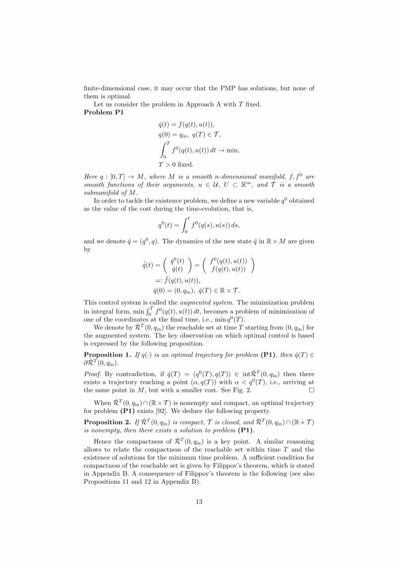
Let us consider the problem in Approach A with T fixed.Problem P1
q(t) = f(q(t), u(t)),
q(0) = qin, q(T ) ∈ T ,∫ T
0
f0(q(t), u(t)) dt→ min,
T > 0 fixed.
Here q : [0, T ] → M , where M is a smooth n-dimensional manifold, f, f0 aresmooth functions of their arguments, u ∈ U , U ⊂ Rm, and T is a smoothsubmanifold of M .
In order to tackle the existence problem, we define a new variable q0 obtainedas the value of the cost during the time-evolution, that is,
q0(t) =
∫ t
0
f0(q(s), u(s)) ds,
and we denote q = (q0, q). The dynamics of the new state q in R×M are givenby
˙q(t) =
(q0(t)q(t)
)=
(f0(q(t), u(t))f(q(t), u(t))
)=: f(q(t), u(t)),
q(0) = (0, qin), q(T ) ∈ R× T .
This control system is called the augmented system. The minimization problem
in integral form, min∫ T
0f0(q(t), u(t)) dt, becomes a problem of minimization of
one of the coordinates at the final time, i.e., min q0(T ).We denote by RT (0, qin) the reachable set at time T starting from (0, qin) for
the augmented system. The key observation on which optimal control is basedis expressed by the following proposition.
Proposition 1. If q(·) is an optimal trajectory for problem (P1), then q(T ) ∈∂RT (0, qin).
Proof. By contradiction, if q(T ) = (q0(T ), q(T )) ∈ intRT (0, qin) then thereexists a trajectory reaching a point (α, q(T )) with α < q0(T ), i.e., arriving atthe same point in M , but with a smaller cost. See Fig. 2.
When RT (0, qin)∩ (R×T ) is nonempty and compact, an optimal trajectoryfor problem (P1) exists [92]. We deduce the following property.
Proposition 2. If RT (0, qin) is compact, T is closed, and RT (0, qin)∩ (R×T )is nonempty, then there exists a solution to problem (P1).
Hence the compactness of RT (0, qin) is a key point. A similar reasoningallows to relate the compactness of the reachable set within time T and theexistence of solutions for the minimum time problem. A sufficient condition forcompactness of the reachable set is given by Filippov’s theorem, which is statedin Appendix B. A consequence of Filippov’s theorem is the following (see alsoPropositions 11 and 12 in Appendix B).
13

Figure 2: The reachable set of the augmented system (area delimited by the redcurve). The target T is represented by the vertical dashed line.
Proposition 3. Consider the Schrodinger equation
iψ(t) =
H0 +
m∑j=1
uj(t)Hj
ψ(t), (9)
where ψ(t) evolves in the unit sphere S2N−1 of CN , the matrices H0, . . . ,Hm
are N × N Hermitian, and u(t) ∈ U . Let ψ0 be the initial condition for ψ(·)and the final target T be closed. Assume that the set U is convex and compact.Then each of the following two optimal control problems admits a solution:
1. T is fixed, RT (qin) intersects T , and the cost function f0 : S2N−1×U → Ris convex;
2. minimum time problem when R(qin) intersects T .
Example 2. The compactness of U is a key assumption to ensure the existenceof an optimal solution. We come back to the example of Sec. 2 and we considerthe control of a two-level quantum system whose dynamics is governed by theHamiltonian H = u ( 0 1
1 0 ) with u real-valued [50]. The goal of the control is tosteer the wave function from ψin = (1, 0) to the target T = (0, eiθ) | θ ∈ Rin minimum time. If U = R then there is no optimal solution since the targetstate can be reached in an arbitrary small time, while the control cannot berealized in a zero time. When U = (−1, 1), the transfer can be achieved in atime larger than π/2, but not exactly in time T = π/2. It is only in the casewhere U is compact, e.g. U = [−1, 1], that an optimal solution exists. We findfor the constraint |u(t)| ≤ 1 a pulse which allows to bring the population fromone level to another in a time T = π/2.
We show in Sec. 8 and Sec. 9 how to use these results in two standardquantum control examples.
14

6 First-order conditions
For a smooth real-valued function of one variable f0 : R → R, first-order op-timality conditions are obtained from the observation that, at points wheredf0
dx 6= 0, the function f0, which is well approximated by its first-order Taylorseries, cannot be optimal since it behaves locally as a non-constant affine func-tion. In this way, one obtains the necessary condition: If x is minimal for f0
then df0
dx (x) = 0. First-order conditions in optimal control are derived in thesame way. We have to require that for a small control variation, there is no costvariation at first order.
More precisely, if J(u(·)) is the value of the cost for a reference admissi-
ble control u(·) (for instance J(u(·)) =∫ T
0f0(q(t), u(t)) dt in Approach A or
J(u(·)) =∫ T
0f0(q(t), u(t)) dt + d(T , q(T )) in Approach B), and v(·) is another
admissible control, one would like to consider a condition of the form
∂J(u(·) + hv(·))∂h
∣∣∣∣h=0
= 0. (10)
But difficulties may arise for the following reasons.We work in an infinite-dimensional space (the space of controls) and hence
condition (10) should be required for infinitely many v(·). It may very wellhappen that if u(·) and v(·) are admissible controls then u(·) + hv(·) is notadmissible for every h close to 0. Think, for instance, to the case in whichm = 1 and U = [a, b]. If u(t) ≡ b is the reference control, then u(t) + hv(t) isnot admissible for any non-zero perturbation v(·) when hv(t) is strictly positive.Hence, one should be very careful in choosing the admissible variations in orderto fulfill the control restrictions. In Approach A, one should restrict only tocontrol variations for which the corresponding trajectory reaches the target.More precisely, if q(·) is the trajectory corresponding to the control u(·) :=u(·) + hv(·), one should add the condition
q(T ) ∈ T , (11)
with T either free or constrained to be the fixed final time depending on theproblem under study. Condition (11) should be considered as a constraint for theminimization problem, which results in the use of Lagrange multipliers (normaland abnormal).
The occurrence of Lagrange multipliers in optimal control is therefore notdue to the fact that the optimization takes place in an infinite-dimensionalspace, but is rather a general feature of constrained minimization problems, asexplained in Sec. 6.1.
6.1 Why Lagrange multipliers appear in constrained op-timization problems
We first recall how to find the minimum of a function of n variables f0(x), wherex = (x1, . . . , xn), under the constraint f(x) = 0, with the method of Lagrangemultipliers. Here f0 and f are two smooth functions Rn → R. We have twocases.
15

Figure 3: Intersection of the set f(x) = 0 (solid line) with the level set of f0
(dashed line). The two gradients ∇f(x) and ∇f0(x) are parallel at x = x.
• If x is a point such that f(x) = 0 with ∇f(x) 6= 0, then the implicit functiontheorem guarantees that x | f(x) = 0 is a smooth hypersurface in a neighbor-hood of x. In this case, a necessary condition for f0 to have a minimum at x isthat the level set of f0 (i.e., the set on which f0 takes a constant value) is nottransversal to the set x | f(x) = 0 at x. See Figure 3.
More precisely, this means that
∃λ ∈ R such that ∇f0(x) = λ∇f(x). (12)
This statement can be proved by assuming, for instance, that ∂xnf(x) 6= 0.
The set x | f(x) = 0 can then be expressed locally around x as xn =g(x1, . . . , xn−1). The requirement that
∂xif(x1, . . . , xn−1, g(x1, . . . , xn−1)) ≡ 0,
i = 1, . . . , n− 1,
∂xif0(x1, . . . , xn−1, g(x1, . . . , xn−1))|x=x = 0,
i = 1, . . . , n− 1,
provides immediately condition (12) with λ =∂xnf
0(x)∂xnf(x) .
Notice that λ could be equal to zero. This case corresponds to the situationin which f0 has a critical point at x even in the absence of the constraint.• If x is a point such that f(x) = 0 with ∇f(x) = 0 then the set x | f(x) = 0could be very complicated in a neighborhood of x (typical examples are a sin-gle point, two crossing curves, . . . but it could be any closed set). In generalthe value of f0 at these points cannot be compared with neighboring pointsby requiring that a certain derivative is zero (think for instance to the casein which x | f(x) = 0 is an isolated point). However, they are candidatesto optimality. As an illustrative example, consider the case where n = 2,f0(x1, x2) = x2
1 + (x2 − 1/4)2, and f(x1, x2) = (x21 + x2
2)(x21 + x2
2 − 1). Thepoint x = (0, 0) is an isolated point for which f(x) = 0 and ∇f(x) = 0.
These results can be rewritten in the following form.
Theorem 4 (Lagrange multiplier rule in Rn). Let f0 and f be two smoothfunctions from Rn to R. If f0 has a minimum at x on the set x | f(x) = 0,then there exists (λ, λ0) ∈ R2 \ (0, 0) such that, setting Λ(x, λ, λ0) = λf(x) +
16

λ0f0(x), we have
∇xΛ(x, λ, λ0) = 0, ∇λΛ(x, λ, λ0) = 0. (13)
To show that this statement is equivalent to what we just discussed, weobserve that the second equality in (13) gives the constraint f(x) = 0. For thefirst equation, we have two cases. If λ0 6= 0 then we can normalize λ0 = −1and we get λ∇xf(x)−∇xf0(x) = 0, i.e., Eq. (12) with the change of notationλ → λ. If λ0 = 0 then λ 6= 0 and we get ∇xf(x) = 0, that is, the second casestudied above.
The quantities λ and λ0 are respectively called Lagrange multiplier and ab-normal Lagrange multiplier. If (x, λ0, λ) is a solution of Eq. (13) with λ0 6= 0(resp., λ0 = 0) then x is called a normal extremal (resp., abnormal extremal).An abnormal extremal is a candidate for optimality and occurs, in particular,when we cannot guarantee (at first order) that the set x | f(x) = 0 is asmooth curve. Abnormal extremals are candidates for optimality regardless ofcost f0. Note that if x is such that ∇xf(x) = 0 and ∇xf0(x) = 0 then x isboth normal and abnormal. This is the case in which x satisfies the first-ordercondition for optimality even without the constraint, but we cannot guaranteethat the constraint is a smooth curve.
In the (infinite-dimensional) case of an optimal control problem, normal andabnormal Lagrange multipliers appear in a very similar way.
6.2 Statement of the Pontryagin Maximum Principle
In this section, we state the first-order necessary conditions for optimal con-trol problems, namely the PMP. The basic idea is to define a new object (thepre-Hamiltonian, see Eq. (14) below) which allows to formulate the Lagrangemultiplier conditions in a simple and direct way.
The theorem is stated in a more general form that unifies and slightly gener-alizes the optimal control problems of Approaches A and B. In particular, we add
to the cost∫ T
0f0(q(t), u(t))dt a general terminal cost φ(q(T )). In Approach A,
we have φ = 0, while in Approach B, φ represents the distance from q(T ) tothe target T . We allow the target T to coincide with M . This corresponds toleaving the final point q(T ) free in Approach B.
Theorem 5. Consider the optimal control problem
q(t) = f(q(t), u(t)),
q(0) = qin, q(T ) ∈ T ,∫ T
0
f0(q(t), u(t)) dt+ φ(q(T )) −→ min,
where
• M is a smooth manifold of dimension n, U ⊂ Rm,
• T is a (non-empty) smooth submanifold of M . It can be reduced to a point(fixed terminal point) or coincide with M (free terminal point),
• f , f0 are smooth,
17

• u ∈ U ,
• q : [0, T ]→M is a continuous curve [74].
Define the function (called pre-Hamiltonian)
H(q, p, u, p0) = 〈p, f(q, u)〉+ p0f0(q, u), (14)
with(q, p, u, p0) ∈ T ∗M × U × R.
(see [70] for a precise definition of T ∗M).If the pair (q, u) : [0, T ] → M × U is optimal, then there exists a never
vanishing continuous pair (p, p0) : [0, T ] 3 t 7→ (p(t), p0) ∈ T ∗q(t)M × R where
p0 ≤ 0 is a constant and such that for almost every (a.e.) t ∈ [0, T ] we have
i) q(t) = ∂H∂p
(q(t), p(t), u(t), p0) (Hamiltonian equation for q);
ii) p(t) = −∂H∂q
(q(t), p(t), u(t), p0) (Hamiltonian equation for p);
iii) the quantity HM (q(t), p(t), p0) := maxv∈U H(q(t), p(t), v, p0) is well-definedand
H(q(t), p(t), u(t), p0) = HM (q(t), p(t), p0)
which corresponds to the maximization condition.
Moreover,
iv) there exists a constant c ≥ 0 such that HM (q(t), p(t), p0) = c on [0, T ],with c = 0 if the final time is free (value of the Hamiltonian);
v) for every v ∈ Tq(T )T , we have 〈p(T ), v〉 = p0〈dφ(q(T )), v〉 (transversalitycondition), where dφ is the differential of the function φ.
Some comments are in order.• A proof of the PMP can be found, for instance, in [28, 27]. An intuitivederivation based on the Lagrange multiplier rule is presented in Section 7.1 inthe case in which T is fixed, the final point is free, and U = Rm.• The covector p is called adjoint state in the control theory literature [70],while p0 is the abnormal multiplier. The quantities p(·) and p0 play the role ofLagrange multipliers for the constrained optimization problem. We point outthe similarity between the expressions of H and of Λ in Th. 4 (with the changeof notation q → x and p→ λ).•A trajectory q(·) for which there exist p(·), u(·), and p0 such that (q(·), p(·), u(·), p0)satisfies all the conditions given by the PMP is called an extremal trajectory andthe 4-uple (q(·), p(·), u(·), p0) an extremal or, equivalently, an extremal lift of q(·).Such an extremal is called normal if p0 6= 0 and abnormal if p0 = 0. It mayhappen that an extremal trajectory q(·) admits both a normal extremal lift(q(·), p1(·), u(·), p0) and an abnormal one (q(·), p2(·), u(·), 0). In this case, wesay that the extremal trajectory q(·) is a non-strict abnormal trajectory. Notethat (as in the finite-dimensional case) abnormal trajectories are candidates foroptimality regardless of the cost. In the finite-dimensional case, they correspondto singularities of the constraint function, while here they correspond to singu-larities of the functional associating with a control v(·) the endpoint at time
18

T of the solution of q(t) = f(q(t), v(t)), q(0) = qin. It is worth noticing thatabnormal extremals do not only appear in pathological cases, but they are oftenpresent in real-world applications, as for instance in the two examples presentedin Sec. 8 and 9.• The PMP is only a necessary condition for optimality. It may very wellhappen that an extremal trajectory is not optimal. The PMP can thereforeprovide several candidates for optimality, only some of which are optimal (oreven none of them if the step of existence has not been verified, see Sec. 5).• Since the equation for p(·) at point ii) of the PMP is linear, if (q(·), p(·), u(·), p0)is an extremal, then for every α > 0, (q(·), αp(·), u(·), αp0) is an extremal as well.As a consequence, some useful normalizations are possible. A typical normal-ization for normal extremals is to require p0 = − 1
2 but other choices are alsopossible.•When there is no final cost (φ = 0), the transversality condition (v) simplifiesto:
〈p(T ), Tq(T )T 〉 = 0. (15)
When the final point is fixed (T = qfi), Tq(T )T is a zero-dimensional manifoldand hence condition (15) is empty. When the final point is free (T = M) thetransversality condition simplifies to p(T ) = p0dφ(q(T )). In local coordinates,we recover that p(T ) is proportional to the gradient of φ evaluated at the pointq(T ). Notice that, since (p(T ), p0) 6= 0, in this case one necessarily has p0 6= 0.
Table 2 gives a list of the possible extremal solutions of the PMP.
Example 3. As a general example in quantum control, we consider a dynamicalsystem governed by Eq. (2) where the goal is to minimize at the fixed final
time T the cost −|〈ψfi|ψ(T )〉|2 + 12
∫ T0
∑mj=1 u
2j (t)dt, where ψfi is a target state
towards which we want to drive the system (up to a global phase) [93]. A directapplication of the PMP shows that the pre-Hamiltonian H can be expressed as:
H(ψ, χ, uj , p0) = <(〈χ|ψ〉) +
p0
2
∑j
u2j
where the adjoint state, denoted here by χ, is an abstract wave function whichcan be chosen so that it belongs to the unit sphere in CN , 〈χ|χ〉 = 1. Sinceψ and χ are complex-valued functions, the pre-Hamiltonian is defined throughthe real part of the scalar product between χ and ψ. The standard definitionused in Th. 5 can be found by introducing the real and imaginary parts of thewave functions. Using Eq. (2), we deduce that
H(ψ, χ, uj , p0) = =(〈χ|H0 +
∑j
ujHj |ψ〉) +p0
2
∑j
u2j (16)
which leads to
iχ(t) = (H0 +
m∑j=1
uj(t)Hj)χ(t),
i.e., χ also satisfies the Schrodinger equation. We stress that this condition isonly true in the bilinear case. A specific equation has to be computed for otherdynamics, such as, e.g., the Gross–Pitaevskii equation [94]. The final conditionχ(T ) is given by the transversality condition v) of the PMP:
χ(T ) = p0〈ψfi|ψ(T )〉ψfi. (17)
19
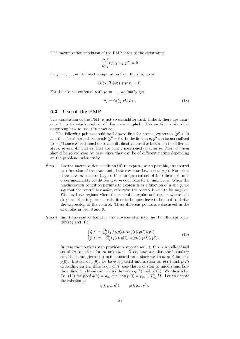
The maximization condition of the PMP leads to the constraints
∂H∂uj
(ψ, χ, uj , p0) = 0
for j = 1, . . . ,m. A direct computation from Eq. (16) gives
=(〈χ|Hj |ψ〉) + p0uj = 0.
For the normal extremal with p0 = −1, we finally get
uj = =(〈χ|Hj |ψ〉). (18)
6.3 Use of the PMP
The application of the PMP is not so straightforward. Indeed, there are manyconditions to satisfy and all of them are coupled. This section is aimed atdescribing how to use it in practice.
The following points should be followed first for normal extremals (p0 < 0)and then for abnormal extremals (p0 = 0). In the first case, p0 can be normalizedto −1/2 since p0 is defined up to a multiplicative positive factor. In the differentsteps, several difficulties (that are briefly mentioned) may arise. Most of themshould be solved case by case, since they can be of different nature dependingon the problem under study.
Step 1. Use the maximization condition iii) to express, when possible, the controlas a function of the state and of the covector, i.e., u = w(q, p). Note thatif we have m controls (e.g., if U is an open subset of Rm) then the first-order maximality conditions give m equations for m unknowns. When themaximization condition permits to express u as a function of q and p, wesay that the control is regular, otherwise the control is said to be singular.We may have regions where the control is regular and regions where it issingular. For singular controls, finer techniques have to be used to derivethe expression of the control. These different points are discussed in theexamples in Sec. 8 and 9.
Step 2. Insert the control found in the previous step into the Hamiltonian equa-tions i) and ii):
q(t) = ∂H∂p (q(t), p(t), w(q(t), p(t)), p0)
p(t) = −∂H∂q (q(t), p(t), w(q(t), p(t)), p0).(19)
In case the previous step provides a smooth w(·, ·), this is a well-definedset of 2n equations for 2n unknowns. Note, however, that the boundaryconditions are given in a non-standard form since we know q(0) but notp(0). Instead of p(0), we have a partial information on q(T ) and p(T )depending on the dimension of T (see the next step to understand howthese final conditions are shared between q(T ) and p(T )). We then solveEq. (19) for fixed q(0) = qin and any p(0) = pin ∈ T ∗qinM . Let us denotethe solution as
q(t; pin, p0), p(t; pin, p
0).
20
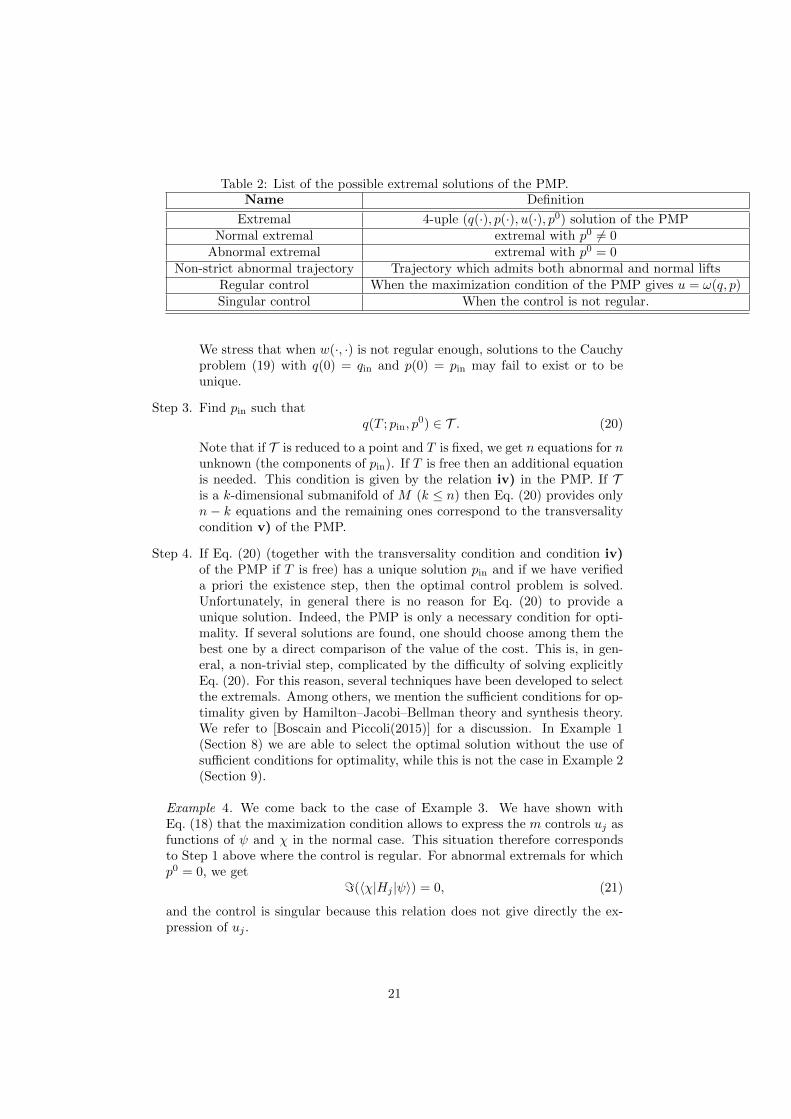
Table 2: List of the possible extremal solutions of the PMP.Name Definition
Extremal 4-uple (q(·), p(·), u(·), p0) solution of the PMPNormal extremal extremal with p0 6= 0
Abnormal extremal extremal with p0 = 0Non-strict abnormal trajectory Trajectory which admits both abnormal and normal lifts
Regular control When the maximization condition of the PMP gives u = ω(q, p)Singular control When the control is not regular.
We stress that when w(·, ·) is not regular enough, solutions to the Cauchyproblem (19) with q(0) = qin and p(0) = pin may fail to exist or to beunique.
Step 3. Find pin such thatq(T ; pin, p
0) ∈ T . (20)
Note that if T is reduced to a point and T is fixed, we get n equations for nunknown (the components of pin). If T is free then an additional equationis needed. This condition is given by the relation iv) in the PMP. If Tis a k-dimensional submanifold of M (k ≤ n) then Eq. (20) provides onlyn − k equations and the remaining ones correspond to the transversalitycondition v) of the PMP.
Step 4. If Eq. (20) (together with the transversality condition and condition iv)of the PMP if T is free) has a unique solution pin and if we have verifieda priori the existence step, then the optimal control problem is solved.Unfortunately, in general there is no reason for Eq. (20) to provide aunique solution. Indeed, the PMP is only a necessary condition for opti-mality. If several solutions are found, one should choose among them thebest one by a direct comparison of the value of the cost. This is, in gen-eral, a non-trivial step, complicated by the difficulty of solving explicitlyEq. (20). For this reason, several techniques have been developed to selectthe extremals. Among others, we mention the sufficient conditions for op-timality given by Hamilton–Jacobi–Bellman theory and synthesis theory.We refer to [Boscain and Piccoli(2015)] for a discussion. In Example 1(Section 8) we are able to select the optimal solution without the use ofsufficient conditions for optimality, while this is not the case in Example 2(Section 9).
Example 4. We come back to the case of Example 3. We have shown withEq. (18) that the maximization condition allows to express the m controls uj asfunctions of ψ and χ in the normal case. This situation therefore correspondsto Step 1 above where the control is regular. For abnormal extremals for whichp0 = 0, we get
=(〈χ|Hj |ψ〉) = 0, (21)
and the control is singular because this relation does not give directly the ex-pression of uj .
21

Applying Step 2, we obtain in the regular situation the following coupledequations for ψ and χ:
iψ = [H0 +∑j =(〈χ|Hj |ψ〉)Hj ]ψ
iχ = [H0 +∑j =(〈χ|Hj |ψ〉)Hj ]χ
(22)
with the boundary conditions ψ(0) = ψin and Eq. (17). In Step 3, we then solveEq. (22) to find the initial condition χ(0) such that the final state χ(T ) satisfiesEq. (17) at time T .
The numerical procedures used to select the initial condition χ(0), calledshooting methods in control theory, are based on suitable adaptations of theNewton algorithm [35, 36]. Step 4 consists finally in comparing the cost of thedifferent solutions found in Step 3.
In the abnormal case, we use the fact that Eq. (21) is satisfied in a non-zerotime interval so the time derivatives of =(〈χ|Hj |ψ〉) are also zero. The first timederivative leads to the m relations
m∑j=1
uj<(〈χ|[Hk, Hj ]|ψ) = <(〈χ|[H0, Hk]|ψ〉),
with k = 1, . . . ,m. This linear system can be expressed in a more compact formas
Ru = s,
where R is a m × m matrix with elements Rkj = <(〈χ|[Hk, Hj ]|ψ) and s avector of coordinates sk = <(〈χ|[H0, Hk]|ψ〉). We deduce that the control u isgiven as a function of ψ and χ as u = R−1s. If this system is singular then thesecond time derivative has to be used. This is the case, e.g., for m = 1, when afurther constraint has to be fulfilled, namely, <(〈χ|[H0, H1]|ψ〉) = 0. From thederivation of u, we then apply Steps 2 and 3 to the abnormal extremals.
7 Gradient-based optimization algorithm
The aim of this section is to introduce a first order gradient-based optimizationalgorithm based on the PMP. We first derive the necessary conditions of thePMP in the case of a fixed control time without any constraint on the finalstate and on the control. This construction is known in control theory as theweak PMP. Note that we consider only the case of regular control. Iterativealgorithms can be deduced from these conditions. In a second step, we applythis idea to quantum control and we show how a gradient-based optimizationalgorithm, GRAPE [45], can be designed from this approach.
7.1 The Weak Pontryagin Maximum Principle
We consider a control system whose dynamics are governed by Eq. (1), whenthe final state is free and the control is unconstrained. The objective is to solvea control problem in the Approach B, as defined in Sec. 3 with a fixed controltime T . We recall that the cost functional to minimize can be expressed as
J(u(·)) =
∫ T
0
f0(q(t), u(t)) dt+ d(T , q(T )).
22

Considering the evolution equation (1) as a dynamical constraint (in infinitedimension), in order to apply (formally) the Lagrange multiplier rule for normalextremals, we introduce the functional
Λ(p(·), u(·)) = d(T , q(T )) +
∫ T
0
f0(q(t), u(t)) dt
+
∫ T
0
〈p(t), q(t)− f(q(t), u(t))〉 dt. (23)
We stress that the Lagrange multiplier p(·) is here a function on [0, T ]. Inte-grating by parts Eq. (23), we obtain
Λ(p(·), u(·)) = d(T , q(T )) + 〈p(T ), q(T )〉− 〈p(0), q(0)〉
−∫ T
0
(H(q(t), p(t), u(t)) + 〈p(t), q(t)〉) dt,
withH(q, p, u) = 〈p, f(q, u)〉 − f0(q, u). (24)
Note that the scalar function H has the same expression (with p0 = −1) as thepre-Hamiltonian H introduced in Sec. 6.2 for the statement of the PMP. Sincethere is no constraint on the control law, i.e., u(t) ∈ Rm for any time t, weconsider the variation δΛ in Λ at first order due to the variation δu of u. Thischange of control induces a variation of the trajectory δq(t) with δq(0) = 0,the initial point being fixed. Note that the adjoint state p is not modified. Wearrive at:
δΛ = 〈 ∂d(T , q)∂q
∣∣∣∣q=q(T )
+ p(T ), δq(T )〉
−∫ T
0
[〈∂H∂q
+ p, δq〉+∂H
∂uδu] dt. (25)
A necessary condition for Λ to be an extremum is δΛ = 0 for any variation δu.A solution is given by taking an adjoint state p satisfying
p = −∂H∂q
, (26)
the final boundary condition
p(T ) = − ∂d(T , q)∂q
∣∣∣∣q=q(T )
, (27)
and requiring∂H
∂u= 0 on [0, T ].
As it could be expected, we find here a weak version of the equations of thePMP introduced in Sec. 6.2 where the maximization of the pre-Hamiltonian isreplaced by an extremum condition given by the partial derivative with respectto u. We point out that this approach works if the set U is open.
23
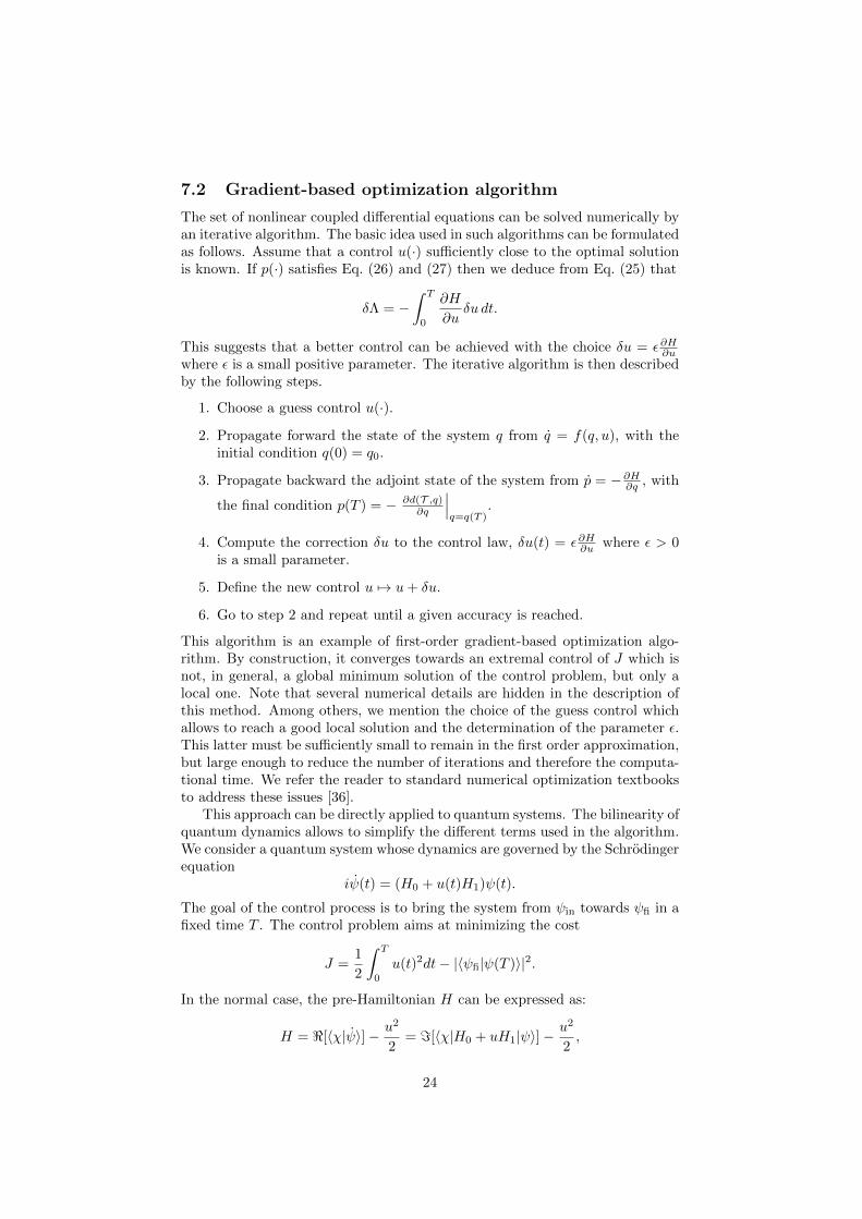
7.2 Gradient-based optimization algorithm
The set of nonlinear coupled differential equations can be solved numerically byan iterative algorithm. The basic idea used in such algorithms can be formulatedas follows. Assume that a control u(·) sufficiently close to the optimal solutionis known. If p(·) satisfies Eq. (26) and (27) then we deduce from Eq. (25) that
δΛ = −∫ T
0
∂H
∂uδu dt.
This suggests that a better control can be achieved with the choice δu = ε∂H∂uwhere ε is a small positive parameter. The iterative algorithm is then describedby the following steps.
1. Choose a guess control u(·).
2. Propagate forward the state of the system q from q = f(q, u), with theinitial condition q(0) = q0.
3. Propagate backward the adjoint state of the system from p = −∂H∂q , with
the final condition p(T ) = − ∂d(T ,q)∂q
∣∣∣q=q(T )
.
4. Compute the correction δu to the control law, δu(t) = ε∂H∂u where ε > 0is a small parameter.
5. Define the new control u 7→ u+ δu.
6. Go to step 2 and repeat until a given accuracy is reached.
This algorithm is an example of first-order gradient-based optimization algo-rithm. By construction, it converges towards an extremal control of J which isnot, in general, a global minimum solution of the control problem, but only alocal one. Note that several numerical details are hidden in the description ofthis method. Among others, we mention the choice of the guess control whichallows to reach a good local solution and the determination of the parameter ε.This latter must be sufficiently small to remain in the first order approximation,but large enough to reduce the number of iterations and therefore the computa-tional time. We refer the reader to standard numerical optimization textbooksto address these issues [36].
This approach can be directly applied to quantum systems. The bilinearity ofquantum dynamics allows to simplify the different terms used in the algorithm.We consider a quantum system whose dynamics are governed by the Schrodingerequation
iψ(t) = (H0 + u(t)H1)ψ(t).
The goal of the control process is to bring the system from ψin towards ψfi in afixed time T . The control problem aims at minimizing the cost
J =1
2
∫ T
0
u(t)2dt− |〈ψfi|ψ(T )〉|2.
In the normal case, the pre-Hamiltonian H can be expressed as:
H = <[〈χ|ψ〉]− u2
2= =[〈χ|H0 + uH1|ψ〉]−
u2
2,
24

where the wave function χ is the adjoint state of the system. We thus deducethat the gradient on which the iterative algorithm is based is given by
∂H
∂u= =[〈χ|H1|ψ〉]− u(t). (28)
We find with Eq. (28) the standard control correction used in the GRAPEalgorithm in quantum control [45].
8 Example 1: A three-level quantum systemwith complex controls
In this section, we mainly use the results of [50], see also [95, 49, 96]. Note, how-ever, that original results concerning the selection of the best extremal amongall the possible solutions are presented.
8.1 Formulation of the quantum control problem
We consider a three-level quantum system whose dynamics are governed by theSchrodinger equation. The system is described by a pure state ψ(t) belongingto a three-dimensional complex Hilbert space. The system is characterized, inthe absence of external fields, by three energy levels E1, E2, and E3 and iscontrolled by the Pump and the Stokes pulses which couple, respectively, statesone and two and states two and three [97]. Note that there is no direct couplingbetween levels one and three. The time evolution of ψ(t) is given by
iψ(t) = H(t)ψ(t),
where
H(t) =
E1 Ω1(t) 0Ω∗1(t) E2 Ω2(t)
0 Ω∗2(t) E3
.
Here Ω1(t),Ω2(t) ∈ C are the two time-dependent complex control parameters.We denote by ψ1(t), ψ2(t), and ψ3(t) the coordinates of ψ(t), that is, ψ(t) =(ψ1(t), ψ2(t), ψ3(t)). They satisfy
|ψ1(t)|2 + |ψ2(t)|2 + |ψ3(t)|2 = 1,
leading to M = S5, a manifold of real dimension 5. The goal of the controlprocess is to transfer population from the first eigenstate to the third one in afixed time T . In other words, the aim is to find a trajectory in M going fromthe submanifold |ψ1|2 = 1 to the one with |ψ3|2 = 1. The system is completelycontrollable thanks to Point 2 in Proposition 9 and the approach A can bechosen. The optimal control problem is defined through the cost functional
C =
∫ T
0
(|Ω1(t)|2 + |Ω2(t)|2)dt,
to be minimized. The cost C can be interpreted as the energy of the controllaws used in the control process. We consider the specific case in which the
25

control parameters are in resonance with the energy transition. More precisely,we assume that the pulses Ω1(t) and Ω2(t) can be expressed as
Ω1(t) = u1(t)ei(E2−E1)t
Ω2(t) = u2(t)ei(E3−E2)t
with u1(t), u2(t) ∈ R to be optimized. Note that this assumption is not restric-tive since it can be shown that the resonant case corresponds to the optimalsolution [50, 95]. The uncontrolled part, called the drift, together with theimaginary unit in the Schrodinger equation, can be eliminated through a uni-tary transformation Y (t) given by
Y (t) = diag(e−iE1t, e−i(E2t+π/2), e−i(E3t+π)).
Defining a new wave function x such that ψ(t) = Y (t)x(t), we obtain thatx(t) solves the Schrodinger equation
ix(t) = H ′(t)x(t),
where H ′ = Y −1HY − iY −1Y . Since Y only modifies the phases of the coordi-nates, ψ(t) and x(t) correspond to the same population distribution, i.e., settingx = (x1, x2, x3) we have |xj(t)|2 = |ψj(t)|2, j = 1, 2, 3.
Computing explicitly H ′ we arrive atx1
x2
x3
=
0 −u1(t) 0u1(t) 0 −u2(t)
0 u2(t) 0
x1
x2
x3
. (29)
Without loss of generality, the optimal control problem can be restricted to thesubmanifold S2 ⊂ M defined by (x1, x2, x3) ∈ R3 | x2
1 + x22 + x2
3 = 1. Thisstatement is trivial if the initial condition belongs to S2 (i.e., if x(0) is real).Otherwise, a straightforward change of phase of the coordinates ψk allows tocome back to this condition. Equation (29) can be expressed in a more compactform as
x = u1(t)F1(x) + u2(t)F2(x), (30)
where
F1(x) =
−x2
x1
0
, F2(x) =
0−x3
x2
.
Notice that F1 and F2 are two vector fields defined on the sphere S2 representing,respectively, a rotation along the x3 axis and along the x1 axis. Since Ω1(t)and Ω2(t) differ from u1(t) and u2(t) only for phase factors, the minimizationproblem becomes
C =
∫ T
0
(u1(t)2 + u2(t)2)dt→ min, (31)
with T fixed. Concerning initial and final conditions, since the goal is to gofrom the submanifold |ψ1|2 = 1 to the submanifold |ψ3|2 = 1, we can assumewithout loss of generality that x(0) = (1, 0, 0) (again, a straightforward changeof coordinates allows to come back to this condition otherwise). Since we arenow restricted to real variables, the target is T = (0, 0,+1), (0, 0,−1). Now,
26

being the target made of two points only, one should compute separately theoptimal trajectories going from (1, 0, 0) to (0, 0, 1) and those going from (1, 0, 0)to (0, 0,−1). Finally between all these trajectories, one should take the oneshaving the smallest cost. Because of the symmetries of the system, the twofamilies of optimal trajectories have precisely the same cost (this will be clear inthe explicit computations later on). As a consequence, without loss of generality,we can fix the final condition as x(T ) = (0, 0, 1).
The problem (30)–(31) with fixed initial and final conditions is actually acelebrated problem in OCT called the Grushin model on the sphere [98, 49, 99].
8.2 Existence
For convenience, let us re-write the optimal control problem as follows:
Problem PGrushin(T )
x = u1(t)F1(x) + u2(t)F2(x),∫ T
0
(u1(t)2 + u2(t)2)dt→ min, T fixed,
x(0) = (1, 0, 0), x(T ) = (0, 0, 1),
u1, u2 ∈ U , U = R.
To prove the existence of solutions to PGrushin(T ), one could be tempted to usePropositions 3 and 11. However u1 and u2 take values in R and, hence, thesecond hypothesis of the proposition is not verified.
Instead, we are going to use the following fact.
Proposition 6. If u1(t), u2(t) are optimal controls for PGrushin(T ), then u1(t)2+u2(t)2 is almost everywhere constant and positive on [0, T ]. Moreover, for everyα > 0, we have that αu1(αt), αu2(αt) are optimal controls for PGrushin(T/α).
To prove this proposition we first state a general lemma for driftless systems.
Lemma 7. Consider a control system of the form x =∑mj=1 uj(t)Fj(x), where
x ∈M and uj ∈ U , j = 1, . . . ,m. Then any admissible trajectory x(·) defined on[0, T ] and corresponding to controls uj(·), j = 1, . . . ,m, is a reparameterizationof an admissible trajectory x(·) defined on the same time interval whose con-
trols uj(·) satisfy a.e.√∑m
j=1 uj(t)2 = L/T , where L =
∫ T0
√∑mj=1 uj(t)
2dt.
Alternatively, x(·) is a reparameterization of a trajectory x(·) defined on [0, L]
whose controls satisfy a.e.√∑m
j=1 uj(t)2 = 1.
We recall that, given an admissible trajectory x : [0, T ] → M , T > 0,corresponding to controls uj(·), j = 1, . . . ,m, a reparameterization of x(·) is atrajectory x(·) = x(τ(·)) with τ : [0, T ]→ [0, T ] a function such that d
dtτ(t) > 0a.e. on [0, T ]. Such trajectory is defined on [0, T ]. Lemma 7 is a consequence of
27

the fact that for a.e. t ∈ [0, T ] we have
˙x(t) =d
dtx(τ(t)) = x(τ(t))τ(t)
=( m∑j=1
uj(τ(t))Fj(x(τ(t)))τ(t)
=
m∑j=1
(uj(τ(t))τ(t)
)Fj(x(t)),
from which it follows that x(·) is admissible and corresponds to controls uj(τ(·))τ(·),j = 1, . . . ,m.
In the following, for the optimal control problem under study, it is convenientto normalize T in such a way that u1(t)2 +u2(t)2 = 1. Usually, when one makesthis choice the trajectories are said to be parameterized by arc length. If theobjective is to reach the target at time T ′, it is sufficient to use the controls(αu1(α t), α u2(α t)), where α = T
T ′ .When T is fixed in such a way that u1(t)2 + u2(t)2 = 1, we call problem
PGrushin(T ) simply PGrushin.Notice that, as a consequence of Lemma 7, if T is not fixed then PGrushin(T )
has no solution. Indeed, assume by contradiction that x(·), defined on [0, T0]and corresponding to controls uj(·), j = 1, 2, is a minimizer for T free. Letc ∈ (0, 1). The trajectory corresponding to controls uj(·) = uj(c ·)c, j = 1, 2, isa reparameterization of x(·) reaching the final point at time T = T0/c with acost ∫ T0
c
0
2∑j=1
uj(ct)2c2dt = c
∫ T0
0
2∑j=1
uj(t)2dt,
<
∫ T0
0
2∑j=1
uj(t)2dt,
which leads to a contradiction.
Proof of Proposition 6. Let us define
L(u(·)) =
∫ T
0
√u1(t)2 + u2(t)2dt,
E(u(·)) =
∫ T
0
(u1(t)2 + u2(t)2)dt.
We are going to use the Cauchy–Schwarz inequality 〈f, g〉2 ≤ ‖f‖2‖g‖2 (withequality holding if and only if f and g are proportional), which holds in anyHilbert space. This inequality simply tells that the scalar product of two vectorsis less than or equal to the product of the norms of the two vectors (with equalityholding iff the two vectors are collinear). In particular, this can be used in the
space L2([0, T ],R) of measurable functions f : [0, T ]→ R with∫ T
0f(t)2 dt <∞.
Namely (∫ T
0
f(t)g(t) dt)2
≤∫ T
0
f(t)2 dt
∫ T
0
g(t)2 dt
28
(with equality holding iff f ∝ g, a.e.). Now, let f(t) =√u1(t)2 + u2(t)2 and
g(t) = 1 for t ∈ [0, T ]. Notice that f, g ∈ U ⊂ L2([0, T ],R). We have
L(u(·))2 ≤ E(u(·))T
(with equality holding iff u1(t)2 + u2(t)2 = const a.e.). Now, let u(·) be a min-imizer of E defined on [0, T ]. Assume by contradiction that u1(t)2 + u2(t)2 isnot a.e. constant. Then L(u(·))2 < E(u(·))T . Let x(·) be an admissible trajec-tory defined on [0, T ] corresponding to controls satisfying
√u1(t)2 + u2(t)2 =
L(u(·))/T a.e., of which x(·) is a reparameterization as in Lemma 7. One im-mediately checks that L(u(·)) = L(u(·)). For this trajectory we have
E(u(·))T = L(u(·))2 = L(u(·))2 < E(u(·))T,
contradicting the fact that u(·) is a minimizer of E.
Now we have the following.
Proposition 8. The problem PGrushin is equivalent to the problem of minimiz-ing time with the constraint on the controls u1(t)2 + u2(t)2 ≤ 1.
Proof. Since for PGrushin we have u1(t)2 + u2(t)2 = 1 a.e., then∫ T
0
(u1(t)2 + u2(t)2)dt = T.
Hence PGrushin is equivalent to the problem of minimizing T with the constrainton the controls u1(t)2 + u2(t)2 = 1. To conclude the proof, let us show that atrajectory corresponding to controls for which the condition
u1(t)2 + u2(t)2 = 1 a.e. (32)
is not satisfied cannot be optimal for the time-optimal control problem men-
tioned in the statement. Actually if (32) is not satisfied then L =∫ T
0
√u1(t)2 + u2(t)2 <
T and an arc length reparameterization of the trajectory reaches the target intime exactly L.
Let us now go back to the problem of existence of optimal trajectories forPGrushin. Thanks to Proposition 8, PGrushin can be equivalently recast as atime-optimal control problem with controls in the convex and compact set U =(u1, u2) ∈ R2 | u2
1 + u22 ≤ 1. We can then apply Propositions 3 and 12 and
deduce the existence of an optimal trajectory for PGrushin (as well as PGrushin(T )for every T > 0).
8.3 Application of the PMP
Before applying the PMP, it is convenient to reformulate the problem inspherical coordinates. Indeed, one can prove the following statement.
Claim. Consider an optimal control problem as in the statement of the PMP(Theorem 5). If all admissible trajectories starting from qin are contained in asubmanifold of M of dimension strictly smaller than n, then each admissibletrajectory has an abnormal extremal lift.
29

Figure 4: (Color online) Picture of the sphere with the spherical coordinates θand ϕ.
This property can be qualitatively justified as follows. We have already men-tioned that abnormal trajectories correspond to singularities of the functionalassociating with a control law the endpoint of the corresponding controlled tra-jectory. If all admissible trajectories starting from qin are contained in a propersubmanifold of M , then the endpoint functional is everywhere singular, meaningthat each admissible trajectory is abnormal.
As a consequence, since in our case all trajectories are contained in thesphere S2, if we apply the PMP in R3 all optimal trajectories admit an abnormalextremal lift. This creates additional difficulties that can be avoided workingdirectly on S2 in spherical coordinates.
Let us introduce the coordinates (θ, ϕ) as displayed in Fig. 4 such that:
x1 = sin θ cosϕ, x2 = cos θ, x3 = sin θ sinϕ.
In these coordinates, the starting point x(0) = (1, 0, 0) and the final pointx(T ) = (0, 0, 1) become (θ, ϕ)(0) = (π/2, 0), (θ, ϕ)(T ) = (π/2, π/2). Noticethat these coordinates are singular for θ = 0 and θ = π but such a singularity
30

does not create any problem, as can be checked by using a second system ofcoordinates around the singularity. The control system takes then the form
θ = −u1(t) cosϕ+ u2(t) sinϕ
ϕ = cot(θ)(u1(t) sinϕ+ u2(t) cosϕ).(33)
It can be simplified by using the controls v1 and v2 defined byv1 = −u1 cosϕ+ u2 sinϕ
v2 = u1 sinϕ+ u2 cosϕ,(34)
which do not modify the expression of the cost C since u21 + u2
2 = v21 + v2
2 . Thecontrol system becomes now(
θϕ
)= v1(t)X1(θ, ϕ) + v2(t)X2(θ, ϕ),
where
X1(θ, ϕ) =
(10
), X2(θ, ϕ) =
(0
cot(θ)
).
Let us now apply the PMP. Set q = (θ, ϕ) and let p = (pθ, pϕ). The pre-Hamiltonian (14) has the form
H(q, p, v, p0)
= v1 〈p,X1(q)〉+ v2 〈p,X2(q)〉+ p0(v21 + v2
2)
= v1pθ + v2pϕ cot(θ) + p0(v21 + v2
2).
We consider the steps of Section 6.3 first for abnormal (p0 = 0) and then fornormal (p0 = − 1
2 ) extremals.
Step 1. In this step, we have to apply the maximization condition to find thecontrol as a function of q and p. Since the controls are unbounded and theHamiltonian is concave, the maximization condition is equivalent to:
∂H∂v1
(q(t), p(t), v(t), p0) ≡ 0∂H∂v2
(q(t), p(t), v(t), p0) ≡ 0.(35)
For abnormal extremals, we obtain〈p(t), X1(q(t))〉 = pθ(t) ≡ 0
〈p(t), X2(q(t))〉 = pϕ(t) cot(θ(t)) ≡ 0.
These conditions do not permit to obtain the control as a function of q and p.Hence, for this problem, abnormal extremals correspond to singular controls.Since p and p0 cannot be simultaneously zero, the only possibility to have anabnormal extremal is that θ(t) ≡ π/2 on [0, T ]. In this case, from Eq. (33), wededuce that ϕ(t) should be constant. As a consequence, an abnormal extremaltrajectory starting from the initial condition (θ, ϕ)(0) = (π/2, 0) will neverreach the final condition (θ, ϕ)(T ) = (π/2, π/2) and we can disregard thesetrajectories.
31
For normal extremals, condition (35) givesv1(t) = 〈p(t), X1(q(t))〉 = pθ(t)
v2(t) = 〈p(t), X2(q(t))〉 = pϕ(t) cot(θ(t)).(36)
Hence, we obtain the controls as a function of q and p and we can conclude thatnormal extremals correspond to regular controls.Step 2. Let us insert (36) into the Hamiltonian equations i) and ii) of Theo-rem 5. We have to consider the case p0 = −1/2 only. We obtain:
θ(t) =∂H∂pθ
(q(t), p(t), v(t),−1/2)
= v1(t) = pθ(t), (37)
pθ(t) = −∂H∂θ
(q(t), p(t), v(t),−1/2)
= v2(t)pϕ(t)(1 + cot(θ(t))2)
= pϕ(t)2 cot(θ(t))(1 + cot2(θ(t))), (38)
ϕ(t) =∂H∂pϕ
(q(t), p(t), v(t),−1/2)
= v2(t) cot(θ(t)) = pϕ(t) cot2(θ(t)), (39)
pϕ(t) = −∂H∂ϕ
(q(t), p(t), v(t),−1/2) = 0. (40)
Equation (40) tells us that pϕ is a constant of the motion, denoted by a in thefollowing. We are then left with the differential equations
θ = pθ, pθ = a2 cot(θ)(1 + cot2(θ)). (41)
Once these are solved, ϕ is obtained by integrating in time equation (39) whichnow has the form
ϕ = a cot2(θ). (42)
Equations (41) and (42) should be solved for every value of a ∈ R with theinitial conditions
θ(0) = π/2, ϕ(0) = 0, pθ(0) = ±1.
The last condition comes from the property that the maximized Hamiltonianis now fixed to 1
2 (corresponding to the choice of taking T in such a way thatoptimal trajectories are parameterized by arc length). More precisely:
1
2= H(q(t), p(t), v(t),−1/2)
= v1(t)pθ(t) + v2(t)a cot(θ(t))
− 1
2(v1(t)2 + v2(t)2)
=1
2(pθ(t)
2 + a2 cot2(θ(t))).
32

Requiring this condition at t = 0, one gets pθ(0) = ±1.The system of equations (41) can be solved using again that the maximized
Hamiltonian is equal to 12 which implies
θ(t)2 = 1− a2 cot2(θ(t)).
Using a separation of variables, we arrive (with the initial condition θ(0) = π/2)at
θ(t) =
arccos(
sin(√
1+a2 t)√1+a2
)if pθ(0) = −1,
π − arccos(
sin(√
1+a2 t)√1+a2
)if pθ(0) = 1.
These expressions lead to a simple formula for x2(t), namely,
x2(t) = ±
(sin(√
1 + a2 t√1 + a2
). (43)
As already explained, the expression for ϕ can be obtained by integrating in timeequation (42) using the expression (6.2) with the initial condition ϕ(0) = 0. Thefinal result is easier expressed in Cartesian coordinates:
x1(t) =a sin(a t) sin
(√1 + a2 t
)√
1 + a2
+ cos(a t) cos(√
1 + a2 t), (44)
x3(t) = sin(a t) cos(√
1 + a2 t)
−a sin
(√1 + a2 t
)cos(a t)
√1 + a2
. (45)
The corresponding controls can be obtained via formulas (37), (38), and(34), or from equation (29), providing
u1(t) = −x1(t)/x2(t) = ± cos(at),
u2(t) = x3(t)/x2(t) = ∓ sin(at).
Step 3. In this step, we have to find the initial covector (i.e., pθ(0) ∈ −1,+1and a = pϕ ∈ R) whose corresponding trajectory arrives at the final target(x1, x2, x3)(T ) = (0, 0, 1).
From expression (43), requiring x2(T ) = 0 we get sin(√
1 + a2 T ) = 0. Thenfrom (44), requiring x1(T ) = 0 we arrive at cos(a T ) = 0. We have then theconditions √
1 + a2T = n1π, aT =π
2+ n2π,
with n1, n2 ∈ Z. Notice that n1 > 0 since T > 0, and hence
a√1 + a2
=n2 + 1
2
n1,
from which we deduce that |n2 + 12 | < n1. It follows that
a =(n2 + 1
2 )/n1√1− (
n2+ 12
n1)2
. (46)
33

The target is reached at time
T = πn1
√1−
(n2 + 1
2
n1
)2
. (47)
Step 4. The previous step provided a discrete set of trajectories reaching thetarget. The ones arriving in shorter time corresponds to n1 = 1 and n2 = 0
or n2 = −1, for which T = π√
32 and a = ±1/
√3. The final expression of the
optimal trajectories and optimal controls arex1(t) = cos3(t/
√3)
x2(t) = ±√
32 sin(2t/
√3)
x3(t) = −ε sin3(t/√
3),
and u1(t) = ± cos(t/
√3)
u2(t) = ∓ε sin(t/√
3),
where ε = ±1 is the sign of a.We point out that the two trajectories arriving at time T at the point (0, 0, 1)
are those corresponding to n2 = 0 (i.e., to a = 1/√
3) and to pθ(0) = ∓1 (i.e.,to the sign + in formula (43)), while the two trajectories arriving at time T atthe point (0, 0,−1) are associated with n2 = −1 (i.e., to a = −1/
√3). See Sec-
tion 8.1. The four trajectories obtained in this way are optimal since we knowthat optimal trajectories exist and the ones that we have selected are the bestamong all trajectories satisfying a necessary condition for optimality. In thisexample, note that we can select the optimal trajectories by applying the PMPand finding by hand the best extremals, without using second order conditionsnor other sufficient conditions for optimality.
Figures 5 and 6 display, respectively, the two symmetric extremal trajecto-ries reaching the target state (0, 0, 1) at time T and the time evolution of thecorresponding controls.
9 Example 2: A minimum time two-level quan-tum system with a real control
9.1 Formulation of the control problem
We consider the control of a spin-1/2 particle whose dynamics are governed bythe Bloch equation in a given rotating frame [100, 101]:
Mx = −ωMy,
My = ωMx − ωx(t)Mz,
Mz = ωx(t)My,
where M = (Mx,My,Mz) is the magnetization vector and ω the offset term.The system is controlled through a single magnetic field along the x axis thatsatisfies the constraint |ωx| ≤ ωmax. We introduce normalized coordinates(x, y, z) = M/M0, where M0 is the thermal equilibrium magnetization, a nor-malized control u = ωx/ωmax which satisfies the constraint |u| ≤ 1, and a
34

0 0.5 1 1.5 2 2.5
0
0.5
1
Figure 5: (Color online) Plot of the two extremal trajectories (in red and blue)on the sphere going from the point (1, 0, 0) to the point (0, 0, 1) and minimizingthe cost functional C.
Figure 6: (Color online) Time evolution of the controls u1 (in black) and u2 (inred). The control time T and the parameter a are respectively set to π
√3/2
and −1/√
3.
35

normalized time τ = ωmaxt (denoted t below). Dividing the previous system byωmaxM0, we get that the time evolution of the normalized coordinates is givenby the equations xy
z
=
−∆y∆x0
+ u(t)
0−zy
,
where ∆ = ωωmax
is the normalized offset. The trajectories of the system lie on
the Bloch sphere defined by the equation x2 + y2 + z2 = 1. The manifold M ishere the sphere S2. The differential system can be written in a more compactform as
q = (F + uG)q, (48)
where q = (x, y, z) is the state of the system, u(t) ∈ U = [−1, 1], and F and Gare the skew-symmetric 3× 3 matrices
F =
0 −∆ 0∆ 0 00 0 0
, G =
0 0 00 0 −10 1 0
.
The vector fields Fq and Gq generate rotations around, respectively, the z andthe x axis.
Existence of time-optimal trajectories. By Point 1 in Proposition 9, anyinitial point q0 on the Bloch sphere M can be connected by an admissibletrajectory of the control system to any other point q1 on the Bloch sphere (seealso [88]). In this case the existence of a time-optimal trajectory connectingq0 to q1 is a direct consequence of Proposition 12 or Proposition 3. Indeed,U = [−1, 1] is compact and the set Fq + uGq | u ∈ U is convex for any pointq of the Bloch sphere.
9.2 Application of the PMP
The goal of the two control processes that we are considering is to steer thesystem in minimum time from the north pole (0, 0, 1) of the Bloch sphere to,respectively, the south pole (0, 0,−1) or the state (1, 0, 0). We follow here theresults established in [48, 102] (see also [103] for an experimental implementa-tion).
The time-optimal control problem is solved by the application of the PMP.Here the cost C to minimize is
C =
∫ T
0
dt = T → min,
where T is free. The pre-Hamiltonian can be expressed as
H(q, p, u, p0) = p(F + uG)q + p0,
where p = (px, py, pz) ∈ R3 is the covector and p0 is a nonpositive constant suchthat p and p0 are not simultaneously equal to 0. (Here p is seen as a row vectorand q as a column vector.) The value of H is constantly equal to 0 since the
36

final time is free. The PMP states that the optimal trajectories are solutions ofthe equations
q(t) =∂H∂p
(q(t), p(t), u(t), p0),
p(t) = −∂H∂q
(q(t), p(t), u(t), p0),
H(q(t), p(t), u(t), p0) = max|v|≤1
H(q(t), p(t), v, p0).
The dynamics of the adjoint state p are given by
p(t) = −p(t)(F + u(t)G). (49)
Note that ddt‖p(t)‖
2 = 0, so that ‖p(t)‖ does not depend on time. Its constantvalue is nonzero since H = 0 and (p, p0) 6= 0.
Steps 1 and 2. Since the only term of the pre-Hamiltonian depending on thecontrol is upGq, the maximization condition of the PMP leads to the introduc-tion of the switching function
Φ(t) = p(t)Gq(t).
In the regular case in which Φ(t) 6= 0, we deduce from the maximization condi-tion that the optimal control is given by the sign of Φ, u(t) = sign[Φ(t)]. Thecorresponding trajectory is called a bang trajectory. If Φ has an isolated zero ina given time interval, then the control function may switch from −1 to 1 or from1 to −1. A bang-bang trajectory is a trajectory obtained after a finite numberof switches.Using the relation (49), we have
Φ(t) = p(t)[G,F ]q(t), (50)
where [·, ·] denotes the matrix commutator operator. In particular, Φ is a C1
function and, for almost every t,
Φ(t) = p(t)[F , [F ,G]]q(t) + u(t)p(t)[G, [F ,G]]q(t).
Since [F , [F ,G]] = −∆2G and [G, [F ,G]] = F , we have, for a.e. t,
Φ(t) = −∆2Φ(t) + u(t)p(t)Fq(t)= −Ω2Φ(t)− p0u(t), (51)
where Ω =√
1 + ∆2 and the second equality follows from the identity H = 0.Abnormal extremals. Abnormal extremals are characterized by the equalityp0 = 0, from which, together withH = 0, we deduce that Φ(t) = −p(t)Fq(t)/u(t).If Φ(t) = 0 at time t, then p(t) is orthogonal both to Fq(t) and Gq(t). If, more-over, t were not an isolated zero of Φ, then Φ(t) = 0, since Φ is C1. It wouldfollow from (50) that p(t) is orthogonal also to [G,F ]q(t). Since for every q ∈Mthe vectors Fq, Gq, and [G,F ]q span the tangent plane TqM to the sphere M ,we would deduce that p(t) = 0, contradicting the PMP. This means that abnor-mal extremals are necessarily bang-bang. Moreover, we deduce from (51) thatthe switching times are the zeros of a nontrivial solution of the equation
Φ + Ω2Φ = 0.
37

The length of an arc between any two successive switching times is then equalto π/Ω.Singular arcs. When the trajectory is normal, there might exist extremals forwhich Φ is zero on a nontrivial time interval. The control is singular on such aninterval, since it cannot directly be obtained from the maximization condition.The restriction of the trajectory to an interval on which Φ ≡ 0 is called a singulararc. Singular arcs are characterized by the fact that the time derivatives of Φ atall orders are zero. Since p(t) is different from zero, the only possibility to havesimultaneously Φ(t) = 0 and Φ(t) = 0 is that the vectors Gq(t) and [G,F ]q(t) areparallel. Since Gq(t) and [G,F ]q(t) generate, respectively, the rotations aroundthe x and the y axis, we deduce that singular arcs are contained in the equatorz = 0 of the sphere. The singular control law us can be calculated from (51) byimposing that Φ and its second time derivative are zero, yielding us(t) = 0. Asit could be expected, this control law generates a rotation along the equator. Itis admissible because |us| ≤ 1.Normal bang-bang extremals. Consider a normal extremal and an interiorbang arc of duration T between the switching times t0 and t0 + T on which thecontrol u is constantly equal to +1 or −1. An interior arc is an arc which isneither at the beginning nor at the end of the extremal. We normalize p0 to−1. According to (51), the function Ψ = Φ− u
Ω2 is a solution of Ψ + Ω2Ψ = 0.Moreover, since Φ is non-constant then Ψ is nontrivial. Hence, Ψ(t) = ν cos(Ωt+θ0) for some ν > 0 and θ0 ∈ R. Moreover, ν > 0 is uniquely identified by u andΦ(t0) through the equalities Ψ(t0) = − u
Ω2 and Ψ(t0) = Φ(t0). Switchings occurif Φ = Ψ + u
Ω2 vanishes and changes sign. Since, moreover, sign[u] = sign[Φ], itfollows that Ψ is larger than the negative value − 1
Ω2 on (t0, t0 +T ) when u = +1and smaller than the positive value 1
Ω2 on (t0, t0 + T ) when u = −1. Hence Tis larger than π/Ω and
Φ(t0 + T ) = −Φ(t0).
If Φ(t0) = 0, we deduce that T = 2π/Ω. Notice that if u is constantly equalto +1 or −1, then the solutions of q = (F + uG)q are 2π/Ω periodic rotationsaround the axis spanned by (u, 0,∆). Since a time-optimal trajectory cannotself-intersect, we conclude that T < 2π/Ω and Φ(t0) 6= 0.
If t0 +T is the starting time of another internal bang arc, then by the aboveconsiderations the duration of such internal bang arc is also equal to T . Given anormal bang-bang trajectory, there exists then T ∈ (π/Ω, 2π/Ω) such that thetrajectory is the concatenation of bang arcs of duration T , except possibly forthe first and last bang arc, whose length can be smaller than T .General extremals. As we have seen in the previous paragraphs, if a trajec-tory contains an internal bang arc, then it is bang-bang. Otherwise the set ofzeros of Φ is connected, that is, either Φ has a single zero or it vanishes on anontrivial singular arc and is different from zero out of it.
To summarize, extremal trajectories are of two types:
• Bang-bang trajectories whose internal bang arcs have all the same lengthT ∈ [π/Ω, 2π/Ω) (the case T = π/Ω corresponding to abnormal extremals)and for which the first and last bang arcs have length at most T .
• Concatenations of a (possibly trivial) bang arc of length smaller that 2π/Ω,a singular arc on which us = 0, and another (possibly trivial) bang arc oflength smaller than 2π/Ω.
38

Steps 3 and 4. We solve in this paragraph two time-optimal control problems.Starting from the north pole (0, 0, 1), the goal is to reach in minimum time thepoints (0, 0,−1) (problem (P1)) and (1, 0, 0) (problem (P2)). To simplify thederivation of the optimal solutions, we assume that |∆| ≤ 1 [48].
Before solving (P1) and (P2), we first derive analytical results describingthe dynamics of the system. Consider a bang extremal trajectory starting fromthe north pole at time t = 0 with control u(t) = ε = ±1. The correspondingtrajectory is given by
x(t) = ε∆Ω2 (1− cos(Ωt))
y(t) = − εΩ sin(Ωt)
z(t) = 1 + 1Ω2 (cos(Ωt)− 1).
The first two times for which z(t) = 0 are t1 = 1Ω (π − arccos(∆2)) and t2 =
1Ω (π + arccos(∆2)). Notice that all other times for which z(t) = 0 are largerthan 2π/Ω and cannot be the duration of a bang arc of an optimal trajectory.
The optimal solution of (P1) is a bang-bang trajectory with a first switchon the equator at t = t1. The total duration of the process is t1 + t2 = 2π
Ω .A symmetric configuration is possible with a first switch at t = t2. The twotrajectories are displayed in Fig. 7. Let us discuss how the optimality of sucha trajectory can be asserted. The proposed trajectory is clearly extremal andconnects the chosen initial and final points. Since a bang-bang trajectory withat least two internal bang arcs has duration larger than 2π/Ω, it follows that anybang-bang trajectory with four or more bang arcs has a duration larger than thecandidate optimal trajectory (that is, 2π
Ω ). One is then left to compare 2πΩ with
finitely many types of trajectories: bang-bang trajectories with two or threebang arcs, and trajectories obtained by concatenation of a bang, a singular, anda bang arc. By setting the initial and final points, this leaves few competitorsto the optimal trajectory, which can be easily excluded by enumeration. As anexample, we consider the concatenation of a bang arc with u = −1, a singulararc and a new bang arc with u = +1. The two bang arcs last for a time t1, while
the duration of the singular arc is 2∆ arctan(
√1−∆2
∆ ). It is then straightforwardto deduce that the duration of this extremal solution is larger than t1 + t2 = 2π
Ω ,except in the case ∆ = 1 for which the singular arc is of length zero.
Let us now discuss the solution of (P2). Using the results of Sec. 9.2, weconsider the concatenation of a bang extremal with u = +1 during the timet1 and of a singular extremal with u = 0 during the time ts. At time t =t1, the trajectory reaches the point (∆,−
√1−∆2, 0). We deduce that ts =
1∆ arctan(
√1−∆2
∆ ). The total duration of the control process is t1 + ts. Thecorresponding trajectory is represented in Fig. 8. One can check that all othercandidates for optimality join (1, 0, 0) in a longer time. The situation is morecomplicated than for (P1), since here ts → ∞ as ∆ → 0, so the candidatetrajectory should be compared with trajectories with more and more bangs as∆ → 0. A proof of the optimality of the trajectory described above can beobtained, for instance, using optimal synthesis theory, i.e., describing all theoptimal trajectories starting from the north pole, as done in [48].
39
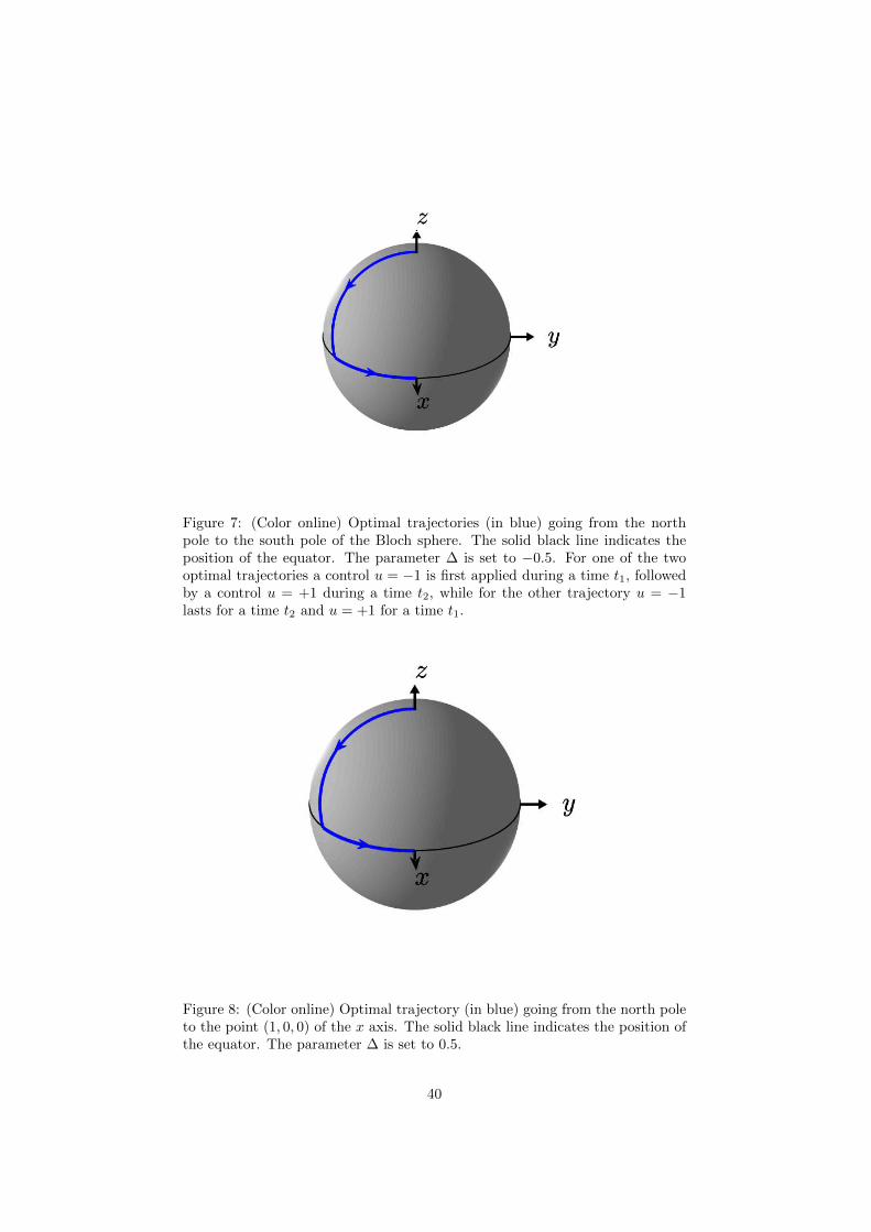
Figure 7: (Color online) Optimal trajectories (in blue) going from the northpole to the south pole of the Bloch sphere. The solid black line indicates theposition of the equator. The parameter ∆ is set to −0.5. For one of the twooptimal trajectories a control u = −1 is first applied during a time t1, followedby a control u = +1 during a time t2, while for the other trajectory u = −1lasts for a time t2 and u = +1 for a time t1.
Figure 8: (Color online) Optimal trajectory (in blue) going from the north poleto the point (1, 0, 0) of the x axis. The solid black line indicates the position ofthe equator. The parameter ∆ is set to 0.5.
40

10 Applications of quantum optimal control the-ory
We discuss in this section the link between the material and results presentedin this tutorial and the current research objectives in this field, both from atheoretical and an experimental points of view. The ability to quickly andaccurately perform operations in a quantum device is a key task in quantumtechnologies. Quantum optimal control theory addresses this challenge by com-bining analytical and numerical tools to design procedures adapted to the ex-perimental setup under study. This approach has the key advantage of beingbased on a rigorous theoretical framework on which all developments have beenbased since the 1980s. In the case of a low-dimensional quantum system as thetwo examples presented in Sec. 8 and 9, the optimal control problem may besolved analytically or at least with a very high numerical accuracy. For high-dimensional systems, an efficient alternative is provided by numerical optimalcontrol procedures, which include first and second-order gradient ascent algo-rithms [45, 66, 104, 105] whose structure is based on the PMP. The connectionbetween the PMP and gradient-based optimization algorithms is described inSec. 7. Their flexibility allows them to adapt to many experimental situationsfor which precise modeling of the dynamics is known. As concrete and recentexamples, we mention the experimental implementation of such techniques inRydberg atoms [106, 107], in spin-wave states of atomic ensembles [108], inelectron spin resonance [109] or in superconducting cavity resonator [110]. Thediversity of these examples shows the key role that optimal control now plays inquantum technologies. We describe below some examples of recent applicationswhich are based on the mathematical formalism described in this tutorial. Wealso indicate some open issues in this field. We stress that our aim is not toprovide an exhaustive list of all optimal control studies in this very active area(we refer the interested reader to recent reviews on this subject [2, 5, 6, 4]), butrather to give an overview of the different aspects that can be analyzed.
The analytical techniques have been applied recently to a series of funda-mental and practical issues in quantum technologies such as robustness [111,112, 113, 114, 115, 116, 117] and selectivity [118, 119] of the control processwith respect to parameters of the system Hamiltonian. The robustness prop-erty is a key factor for the experimental implementation of open-loop optimalpulses. The basic idea consists in controlling simultaneously an ensemble ofidentical systems which differ only by the value of the unknown parameter. Ro-bust or selective optimal pulses are obtained respectively in the case where thetarget states are the same or are different according to the systems. In thesame direction, numerical optimal control has been also employed to improvethe estimation of Hamiltonian parameters [120, 121]. Here, from a specific costfunctional, the control is used to optimize the discrimination between the systemdynamics, which leads to a precise characterization of the Hamiltonian [122].Using the same type of approach, optimal control has proven to be very effectivefor quantum sensing [123, 23, 124].
A key aspect of quantum technologies is the minimum time to perform agiven operation. Lower bounds on the time can be established in the frame-work of quantum speed limits [13, 125] where the time is expressed as a ratiobetween the distance to the target state and the dynamical speed of evolution.
41

Time-optimal trajectories correspond by definition to the speed limit of the pro-cesses. The solutions of the two examples solved in this tutorial give thereforethe quantum speed limits of the problems under study. However, in a higherdimensional quantum system, the many local minima of the control landscapemake it very difficult to find a good approximation of the optimal trajectoryand lead generally to an upper bound of the minimum time. Recent studieshave explored the link between these two formalisms [54, 126]. A major stepforward would be to rigorously describe the concept of speed limit in terms ofthe Pontryagin Maximum Principle [127, 128].
Quantum thermodynamics is nowadays a very useful tool to describe the dy-namics of open quantum systems used in quantum technologies [129]. Optimalcontrol and the PMP can be applied to analyze many issues in this field suchas the enhancement of quantum engine performances [130, 131], work extrac-tion [132, 133] or qubit purification [136, 134, 135]. The quantification of theressources to control a quantum system has been also discussed and could beoptimized from the PMP [137].
An intense effort is being made to develop new quantum optimal control al-gorithms, which are well suited to experimental limitations and constraints [138,139, 140, 141, 142] or which are particularly effective in designing optimalpulses [67, 143, 144]. In particular, hybrid optimal control using feedback fromthe experiment has been developed to avoid problems due to inaccuracies inthe modeling of the dynamics. The structure of the control landscape for thepreparation of quantum many-body systems has been identified and exhibitsa spin-glass-like phase transition in the space of control protocols close to theoptimal fidelity [145]. This structure explains the difficulty to find numericallythe optimal solution in this region. Combining optimal control and machinelearning approaches as proposed in [146] could be a way to solve this problemand to improve the efficiency of optimal algorithms [147, 148]. However, westress that a rigorous mathematical description of these numerical methods andresults will be necessary in the future to systematically apply these approachesto other quantum devices.
We conclude this section by pointing out that the PMP may also play amore unexpected role in quantum computing. It has recently been shown thatGrover’s quantum search problem can be mapped to a time-optimal controlproblem, and then described through the PMP [149]. A connection betweenoptimal control theory and variational quantum algorithms [150] has been es-tablished in [151]. A general description of this intrinsic link is given in [152]where optimal control is used to precisely adjust the parameters of a quantumcircuit. These results highlight that the PMP as a general optimization tool isnot only interesting for the computation of time-dependent control pulses, butalso in other optimization problems of interest in quantum technologies.
11 Conclusion
In this tutorial, we have attempted to give the reader a minimal backgroundon the mathematical techniques of OCT. In our opinion, this is a fundamentalprerequisite to rigorously and correctly apply these tools in quantum control.
The objectives of the tutorial are twofold. First, we have highlighted thekey concepts of the PMP using ideas based on the finding of extrema of func-
42

Table 3: Main notations used in the paper.Notation Definition Section
q(t) the state of the system at time t Sec. 3f a smooth vector-valued function of q and u which defines the control system Sec. 3f0 a smooth scalar-valued function of q and u which defines the cost functional Sec. 3M the manifold on which the state q(t) evolves Sec. 3T the final control time Sec. 3u(t) the value of the control law at time t Sec. 3U the set of possible values of u(t) Sec. 3U the set of admissible control laws Sec. 3T the set of target states Sec. 3
d(T , q(T )) the distance between T and the final state q(T ) Sec. 3R(qin) the set of reachable states from qin Sec. 3RT (qin) the set of reachable states in time T from qin Sec. 3
F(q) the set of directions f(q, u) at q as u varies in U Sec. 5φ(q(T )) the terminal cost which depends on the final state q(T ) Sec. 5J(u(·)) the value of the cost for a control u(·) Sec. 6H the pre-Hamiltonian in the PMP Sec. 6p the adjoint state in the PMP Sec. 6p0 the abnormal multiplier Sec. 6
tions of several variables. This analogy gives non-experts an intuition of thetools of optimal control that might seem abstract on first reading. We havethen stated the PMP and described in details the different steps to be followedin order to solve an optimal control problem. Some are rarely discussed inquantum control, such as the existence of solutions or abnormal and singularextremals, while they play a crucial role in some problems. The link betweenthe PMP and gradient-based optimization algorithms has been explained, whichalso highlights the role of such mathematical tools in any numerical optimiza-tion process. Second, we have solved two basics control problems, namely thecontrol of a three-level quantum system by means of two complex resonant fieldsand the control of a spin 1/2 particle through a real off-resonance driving. Thelow dimension of the two systems allows us to express analytically the optimalsolutions and to give a complete geometric description of the control protocol.Such examples can be used as a starting point by the reader to apply the PMPto more complex quantum systems. A series of recent results using OCT hasbeen briefly discussed to highlight current research directions in this area.
12 List of notations
We provide in Tab. 3 a list of the main notations used in the paper as well asthe first section where they appear or are defined.
43

A Test of controllability
We give in this section a general and useful sufficient condition for controllability.This section completes the discussion of Sec. 3.
Proposition 9. Let M be a smooth manifold and U be a subset of Rm con-taining a neighborhood of the origin. Consider a control system of the formq = F0(q) +
∑mj=1 uj(t)Fj(q), with F0, . . . , Fm smooth vector fields on M and
u(t) = (u1(t), . . . , um(t)) ∈ U . Let L0 be the Lie algebra generated by the vec-tor fields F0, . . . , Fm and L1 be the Lie algebra generated by the vector fieldsF1, . . . , Fm. The system is controllable if at least one of the following conditionsis satisfied:
1. F0 is a recurrent vector field and dim(L0(q)) is equal to the dimension ofM at every q ∈M ;
2. U = Rm and dim(L1(q)) is equal to the dimension of M at every q ∈M .
For a definition of Lie algebra generated by a set of vector fields and forthe notion of recurrent vector field we refer to [28, 89]. For our purposes, it issufficient to recall that:- if F0(q) = A0q, . . . , Fm(q) = Amq are linear vector fields then G ∈ L0 if andonly if G(q) = Bq with B in the matrix Lie algebra (for the commutator prod-uct) generated by A0, . . . , Am;- if a vector field F is such that every solution of q = F (q) is periodic, then Fis recurrent.With these sufficient conditions, we recover the standard controllability condi-tions introduced in quantum control for closed systems [87, 88] and recalled inSec. 3.
B Filippov’s theorem
We state here Filippov’s theorem, which gives a sufficient condition for thecompactness of the reachable set [26]. This section completes the discussion ofSec. 5.
Theorem 10 (Filippov). Fix T > 0. Consider the control system q(t) =f(q(t), u(t)), q ∈M , u ∈ U , where M is a n-dimensional manifold and U ⊂ Rm.Fix an initial condition qin ∈M . Assume the following conditions:
• the set U is compact,
• the set F(q) =f(q, u) | u ∈ U
is convex for every q ∈M ,
• for every u ∈ U , the solution of q(t) = f(q(t), u(t)), q(0) = qin, is definedon the whole interval [0, T ].
Then the sets RT (qin) and R≤T (qin) are compact.
Here R≤T (qin) denotes the reachable set from qin within time T , i.e., the setof points q in M such that there exist T ′ ∈ [0, T ] and an admissible trajectoryq : [0, T ′]→M such that q(0) = qin and q(T ′) = q.
44

Note that the third hypothesis of Th. 10 is automatically satisfied when Mis compact.
By applying Filippov’s theorem to the augmented system for problem (P1)introduced in Sec. 5, one obtains:
Proposition 11. Fix T > 0. Assume that
• T is closed and RT (qin) ∩ T 6= ∅,
• the set U is compact,
• the set F(q) =
(f0(q, u)f(q, u)
)| u ∈ U
is convex for every q ∈M ,
• for every u ∈ U the solution of q(t) = f(q(t), u(t)), q(0) = qin, is definedon the whole interval [0, T ].
Then there exists a solution to problem P1.
Example 5. The conclusion of Proposition 11 may fail to hold if we drop theconvexity assumption on the set F(q) of admissible velocities, as illustrated bythe following example. Take M = R2, U = −1, 1, and f(q, u) = Auq withA1 =
(−1 1−1 0
)and A−1 =
(−1 −11 0
). We point out that the corresponding control
system satisfies all the assumptions of Th. 10 except for the convexity of F(q),since the control can only take two discrete values −1 and 1. Pick qin = (1, 0)and any T > 0. Then qT := e−T qin is in the closure of RT (qin), since we canend up arbitrarily close to qT at time T by applying a control that switchesfast enough between −1 and 1. On the other hand, if q(t) = f(q(t), u(t)) attime t and q(t) has a nonzero vertical component, then d
dt‖q(t)‖ > −‖q(t)‖.Since every trajectory of the control system starting at qin necessarily leaves thehorizontal axis, its final point at time T has norm larger than e−T . ConsequentlyqT 6∈ RT (qin). This proves that RT (qin) is not closed, hence the conclusion ofTh. 10 does not hold. This result is illustrated in Fig. 9 which shows numericallythat the distance to the target state tends to zero when the number of switchesgoes to +∞. This example also highlights possible numerical problems when theexistence of the optimal solution is not verified. Here, an optimization algorithmcannot converge towards a well-defined control law.
The idea of reducing the problem of existence of an optimal control to thecompactness of the reachable set of the augmented system can be used for moregeneral problems. For instance, if we add a terminal cost φ(q(T )) to the cost∫ T
0f0(q(t), u(t)) dt, where φ is a smooth function (as for instance in Approach
B, or in the general formulation given in Sec. 6.2), we get a similar resultadding to f0(q(t), u(t)) the directional derivative of φ along f(q(t), u(t)), thatis, replacing f0(q(t), u(t)) by f0(q(t), u(t)) + 〈dφ(q(t)), f(q(t), u(t))〉. We recallthat here dφ(q(t)) denotes the differential of φ evaluated at q(t) and that 〈·, ·〉is the duality product between covectors of T ∗M and vectors of TM .
When the final time is free, it is more difficult to get the existence of optimaltrajectories. However, the compactness ofR≤T (qin) in the Filippov theorem canbe used to find conditions for the existence of optimal controls in minimum time.We state this result in the case where M is compact. Note that the problemof minimizing time can be written in the form of problem P1 with T free andf0 = 1.
45

10 30 50 70 900
0.02
0.04
0.06
0.08
0 0.2 0.4 0.6 0.8 1
-1
0
1
Figure 9: Illustration of the existence problem. Panels (a) and (b) depict re-spectively the Euclidian distance d to the target as a function of the number Nsof switchings and an example of control law u with Ns = 8.
46

Proposition 12. Consider problem P1 with T free, f0 = 1, and M compact.Assume that
• T is closed and R(qin) ∩ T 6= ∅,
• the set U is compact,
• the set F(q) = f(q, u) | u ∈ U is convex for every q ∈M .
Then there exists a solution to the problem.
A straightforward application of Propositions 11 and 12 to closed quantumsystems yields Proposition 3 of the main text.
Acknowledgments
The authors have contributed equally to this work. This research has been par-tially supported by the ANR projects “SRGI” ANR-15-CE40-0018 and “QUACO”ANR-17-CE40-0007-01. This project has received funding from the EuropeanUnion Horizon 2020 research and innovation program under Marie-Sklodowska-Curie Grant No. 765267 (QUSCO). We gratefully acknowledge useful discus-sions with Pr. Christiane Koch, who suggested us to write this tutorial andprovided advice throughout the project. We thank the PhD students J. Fis-cher, L. Kerber, M. Krauss, J. Langbehn, A. Marshall, and F. Roy for theirhelpful comments.
References
[1] A. Acin, I. Bloch, H. Buhrman, T. Calarco, C. Eichler, J. Eisert, D. Esteve,N. Gisin, S. J. Glaser, F. Jelezko, et al., New Journal of Physics 20, 080201(2018).
[2] S. J. Glaser, U. Boscain, T. Calarco, C. P. Koch, W. Kockenberger,R. Kosloff, I. Kuprov, B. Luy, S. Schirmer, T. Schulte-Herbruggen, et al.,European Physical Journal D 69, 279 (2015).
[3] D. D’Alessandro, Introduction to quantum control and dynamics. (AppliedMathematics and Nonlinear Science Series. Boca Raton, FL: Chapman,Hall/CRC., 2008).
[4] C. Brif, R. Chakrabarti, and H. Rabitz, New Journal of Physics 12, 075008(2010).
[5] C. Altafini and F. Ticozzi, IEEE Trans. Automat. Control 57, 1898 (2012),ISSN 0018-9286.
[6] D. Dong and I. R. Petersen, IET Control Theory & Applications 4, 2651(2010).
[7] C. P. Koch, Journal of Physics: Condensed Matter 28, 213001 (2016).
[8] D. Guery-Odelin, A. Ruschhaupt, A. Kiely, E. Torrontegui, S. Martınez-Garaot, and J. G. Muga, Rev. Mod. Phys. 91, 045001 (2019).
47
[9] N. V. Vitanov, A. A. Rangelov, B. W. Shore, and K. Bergmann, Rev.Mod. Phys. 89, 015006 (2017).
[10] C. P. Koch, M. Lemeshko, and D. Sugny, Rev. Mod. Phys. 91, 035005(2019).
[11] D. Daems, A. Ruschhaupt, D. Sugny, and S. Guerin, Phys. Rev. Lett.111, 050404 (2013).
[12] G. T. Genov, D. Schraft, T. Halfmann, and N. V. Vitanov, Phys. Rev.Lett. 113, 043001 (2014).
[13] S. Deffner and S. Campbell, Journal of Physics A: Mathematical andTheoretical 50, 453001 (2017).
[14] H. Wakamura and T. Koike, New Journal of Physics 22, 073010 (2020).
[15] D. C. Brody and D. M. Meier, Phys. Rev. Lett. 114, 100502 (2015).
[16] A. Carlini, A. Hosoya, T. Koike, and Y. Okudaira, Phys. Rev. Lett. 96,060503 (2006).
[17] X. Wang, M. Allegra, K. Jacobs, S. Lloyd, C. Lupo, and M. Mohseni,Phys. Rev. Lett. 114, 170501 (2015).
[18] A. Ruschhaupt, X. Chen, D. Alonso, and J. G. Muga, New Journal ofPhysics 14, 093040 (2012).
[19] S. Lloyd and S. Montangero, Phys. Rev. Lett. 113, 010502 (2014).
[20] F. K. Wilhelm, S. Kirchhoff, S. Machnes, N. Wittler, and D. Sugny, Lec-ture notes for the 51st IFF Spring School (2020).
[21] J. P. Palao and R. Kosloff, Phys. Rev. Lett. 89, 188301 (2002).
[22] J. Geng, Y. Wu, X. Wang, K. Xu, F. Shi, Y. Xie, X. Rong, and J. Du,Phys. Rev. Lett. 117, 170501 (2016).
[23] P. Rembold, N. Oshnik, M. M. Muller, S. Montangero, T. Calarco, andE. Neu, AVS Quantum Science 2, 024701 (2020).
[24] T. Schaetz, C. R. Monroe and T. Esslinger, New J. Phys. 15, 085009(2013)
[25] P. Doria, T. Calarco, and S. Montangero, Phys. Rev. Lett. 106, 190501(2011).
[26] D. Liberzon, Calculus of variations and optimal control theory (PrincetonUniversity Press, Princeton, NJ, 2012).
[27] L. S. Pontryagin, V. Boltianski, R. Gamkrelidze, and E. Mitchtchenko,The Mathematical Theory of Optimal Processes (John Wiley and Sons,New York, 1962).
[28] A. A. Agrachev and Y. L. Sachkov, Control theory from the geometricviewpoint, vol. 87 of Encyclopaedia of Mathematical Sciences (Springer-Verlag, Berlin, 2004).
48

[29] A. Agrachev, D. Barilari, and U. Boscain, A comprehensive introductionto sub-Riemannian geometry, vol. 181 of Cambridge Studies in AdvancedMathematics (Cambridge University Press, Cambridge, 2020).
[30] A. Bressan and B. Piccoli, Introduction to the mathematical theory of con-trol, vol. 2 of AIMS Series on Applied Mathematics (American Instituteof Mathematical Sciences (AIMS), Springfield, MO, 2007).
[31] H. Schattler and U. Ledzewicz, Geometric optimal control, vol. 38 of In-terdisciplinary Applied Mathematics (Springer, New York, 2012).
[32] U. Boscain and B. Piccoli, Optimal syntheses for control systems on 2-Dmanifolds, vol. 43 of Mathematiques & Applications (Berlin) [Mathematics& Applications] (Springer-Verlag, Berlin, 2004).
[33] V. Jurdjevic, Geometric control theory, vol. 52 of Cambridge Studies inAdvanced Mathematics (Cambridge University Press, Cambridge, 1997),ISBN 0-521-49502-4.
[34] M. M. Lee and L. Markus, Foundations of Optimal Control Theory (JohnWiley and Sons, New York, 1967).
[35] B. Bonnard and D. Sugny, Optimal Control in Space and Quantum Dy-namics (American Institute of Mathematical Sciences, Springfield, MO,2012), Vol. 5.
[36] A. E. Bryson and Y. C. Ho, Applied Optimal Control: Optimization, Es-timation, and Control (Taylor and Francis, Philadelphia, 1975).
[37] A. P. Peirce, M. A. Dahleh, and H. Rabitz, Phys. Rev. A 37, 4950 (1988).
[38] R. Kosloff, S. Rice, P. Gaspard, S. Tersigni, and D. Tannor, ChemicalPhysics 139, 201 (1989), ISSN 0301-0104.
[39] S. A. Rice and M. Zhao, Optimal Control of Molecular Dynamics (JohnWiley and Sons, New York, 2000).
[40] J. Somloi, V. A. Kazakov, and D. J. Tannor, Chemical Physics 172, 85(1993), ISSN 0301-0104.
[41] L. Levin, W. Skomorowski, L. Rybak, R. Kosloff, C. P. Koch, and Z. Ami-tay, Phys. Rev. Lett. 114, 233003 (2015).
[42] D. Sugny, A. Keller, O. Atabek, D. Daems, C. M. Dion, S. Guerin and H.Jauslin, Phys. Rev. A 71, 063402 (2005)
[43] S. Conolly, D. Nashimura, and A. Macovski, IEEE Trans. Med. Imag. 5,106 (1986).
[44] T. E. Skinner, T. O. Reiss, B. Luy, N. Khaneja, and S. J. Glaser, Journalof Magnetic Resonance 163, 8 (2003).
[45] N. Khaneja, T. Reiss, C. Kehlet, T. Schulte-Herbrueggen, and S. J. Glaser,Journal of Magnetic Resonance 172, 296 (2005), ISSN 1090-7807.
49

[46] K. Kobzar, S. Ehni, T. E. Skinner, S. J. Glaser, and B. Luy, Journal ofMagnetic Resonance 225, 142 (2012), ISSN 1090-7807.
[47] D. D’Alessandro and M. Dahleh, IEEE Transactions on Automatic Con-trol 46, 866 (2001).
[48] U. Boscain and P. Mason, J. Math. Phys. 47, 062101, 29 (2006).
[49] U. Boscain, T. Chambrion, and G. Charlot, Discrete Contin. Dyn. Syst.Ser. B 5, 957 (2005).
[50] U. Boscain, G. Charlot, J.-P. Gauthier, S. Guerin, and H.-R. Jauslin, J.Math. Phys. 43, 2107 (2002a).
[51] A. Garon, S. J. Glaser, and D. Sugny, Phys. Rev. A 88, 043422 (2013).
[52] N. Khaneja, R. Brockett, and S. J. Glaser, Phys. Rev. A 63, 032308(2001).
[53] N. Khaneja, S. J. Glaser, and R. Brockett, Phys. Rev. A 65, 032301(2002).
[54] G. C. Hegerfeldt, Phys. Rev. Lett. 111, 260501 (2013).
[55] D. Stefanatos, J. Ruths, and J.-S. Li, Phys. Rev. A 82, 063422 (2010).
[56] X. Chen, Y. Ban, and G. C. Hegerfeldt, Phys. Rev. A 94, 023624 (2016).
[57] N. Khaneja, B. Luy, and S. J. Glaser, Proceedings of the NationalAcademy of Sciences 100, 13162 (2003).
[58] S. E. Sklarz, D. J. Tannor, and N. Khaneja, Phys. Rev. A 69, 053408(2004).
[59] M. Lapert, Y. Zhang, M. Braun, S. J. Glaser, and D. Sugny, Phys. Rev.Lett. 104, 083001 (2010).
[60] B. Bonnard, M. Chyba, and D. Sugny, IEEE Transactions on AutomaticControl 54, 2598 (2009).
[61] B. Bonnard, O. Cots, S. J. Glaser, M. Lapert, D. Sugny, and Y. Zhang,IEEE Transactions on Automatic Control 57, 1957 (2012).
[62] D. Stefanatos, N. Khaneja, and S. J. Glaser, Phys. Rev. A 69, 022319(2004).
[63] M. Lapert, E. Assemat, S. J. Glaser, and D. Sugny, Phys. Rev. A 88,033407 (2013).
[64] V. Mukherjee, A. Carlini, A. Mari, T. Caneva, S. Montangero, T. Calarco,R. Fazio, and V. Giovannetti, Phys. Rev. A 88, 062326 (2013).
[65] D. M. Reich, M. Ndong, and C. P. Koch, The Journal of Chemical Physics136, 104103 (2012).
[66] S. Machnes, U. Sander, S. J. Glaser, P. de Fouquieres, A. Gruslys,S. Schirmer, and T. Schulte-Herbruggen, Phys. Rev. A 84, 022305 (2011).
50

[67] S. Machnes, E. Assemat, D. Tannor, and F. K. Wilhelm, Phys. Rev. Lett.120, 150401 (2018).
[68] A. Borzı, G. Ciaramella, and M. Sprengel, Formulation and numericalsolution of quantum control problems, vol. 16 of Computational Science& Engineering (Society for Industrial and Applied Mathematics (SIAM),Philadelphia, PA, 2017).
[69] U. Boscain, J.-P. Gauthier, F. Rossi, and M. Sigalotti, Comm. Math.Phys. 333, 1225 (2015), ISSN 0010-3616.
[70] When not specified differently, we consider in this paper manifolds withoutboundary. Recall that the tangent space TqM at a point q of a smoothmanifold M is the vector space of all the vectors tangent to M at q. Thetangent bundle TM is the set of all the tangent spaces at any q ∈M . Atevery point q ∈M one can also attach the cotangent space T ∗qM , which isthe dual space to TqM . An element p of T ∗qM is called a covector and isa scalar-valued linear function on TqM , whose value at a vector v ∈ TqMis denoted by 〈p, v〉 and referred to as the duality product between p andv. The collection of the cotangent spaces at all points of M forms thecotangent bundle T ∗M . If M has dimension n, p ∈ T ∗qM , and v ∈ TqM ,in local coordinates, one can think of p as a row vector and v as a columnvector, so that the duality product 〈p, v〉 is equal to pv.
[71] The class of admissible controls is the space U = L∞([0, T ], U), i.e., thespace of measurable and essentially bounded functions from [0, T ] to U .Recall that a function u : [0, T ] → U is said to be essentially bounded ifthere exists a set ω ⊂ [0, T ] of measure zero such that u is bounded on[0, T ] \ ω.
[72] The reason is that a minimizing sequence of piecewise constant controlsmay fail to have a cluster point in the class (intervals on which the controlis constant may have zero duration at the limit). For this reason, optimalcontrol problems are set for a larger class of controls in which optimalsolutions can be shown to exist (under rather general conditions that wediscuss in the main text) and can be characterized through suitable nec-essary conditions. Such conditions often allow to ensure that the optimalcontrols are indeed piecewise continuous. We should stress, however, thatthere exist some examples, such as the Fuller problem [73], for which theoptimal control law has infinitely many switches between two values of Uin finite time. Such a control law is not piecewise continuous, but belongsto L∞([0, T ], U).
[73] A. T. Fuller, Int. J. Control 41, 1 (1985).
[74] The unique solution q(·) of Eq. (1) is locally Lipschitz continuous. A locallyLipschitz continuous curve q(·) for which there exists an admissible controlu(·) such that Eq. (1) is satisfied is said to be an admissible trajectory.Recall that, given an interval I ⊂ R, a function q : I → M is said to beLipschitz continuous if there exists C > 0 such that for every t1, t2 ∈ I thedistance in M between q(t1) and q(t2) is at most C|t1 − t2|, while q(·) issaid to be locally Lipschitz continuous if for every t ∈ I there exists ε > 0such that the restriction of q to I ∩ (t− ε, t+ ε) is Lipschitz continuous.
51

[75] M. Lapert, R. Tehini, G. Turinici, and D. Sugny, Phys. Rev. A 78, 023408(2008).
[76] Y. Ohtsuki and K. Nakagami, Phys. Rev. A 77, 033414 (2008).
[77] V. Gorini, A. Kossakowski, and E. C. G. Sudarshan, J. Math. Phys. 17,821 (1976).
[78] G. Lindblad, Commun. Math. Phys. 48, 119 (1976).
[79] R. Alicki and K. Lendi, Quantum Dynamical Semigroups (Springer,Berlin, 1987).
[80] G. L. Giorgi, A. Saharyan, S. Guerin, D. Sugny and B. Bellomo, Phys.Rev. A 101, 012122 (2020)
[81] H.-P. Breuer and F. Petruccione, The theory of open quantum systems(Oxford University, Oxford, 2002).
[82] S. G. Schirmer and A. I. Solomon, Phys. Rev. A 70, 022107 (2004).
[83] S. G. Schirmer, T. Zhang, and J. V. Leahy, Journal of Physics A: Mathe-matical and General 37, 1389 (2004).
[84] Notice that even if M is here a manifold with a boundary ∂M , the forwardtime dynamics are well defined because the admissible velocities at anypoint of ∂M are either directed towards the interior of M or are tangentto ∂M [86].
[85] Given a manifold M of dimension n, a submanifold of M of dimensionm ≤ n is a subset of M which locally looks like Rm.
[86] C. Altafini, Phys. Rev. A 70, 062321 (2004).
[87] F. Albertini and D. D’Alessandro, IEEE Trans. Automat. Control 48,1399 (2003), ISSN 0018-9286.
[88] S. G. Schirmer, H. Fu, and A. I. Solomon, Phys. Rev. A 63, 063410 (2001).
[89] U. Boscain and M. Sigalotti, in Contemporary research in elliptic PDEsand related topics (Springer, Cham, 2019), vol. 33 of Springer INdAMSer., pp. 203–219.
[90] C. Altafini, J. Math. Phys. 44, 2357 (2003).
[91] G. Dirr, U. Helmke, I. Kurniawan, and T. Schulte-Herbrueggen, Rep.Math. Phys. 64, 93 (2009).
[92] Note that this statement can be deduced at once by taking any convergingsubsequence of a minimizing sequence.
[93] J. Werschnik and E.K.U. Gross, J. Phys. B 40, 175 (2007).
[94] U. Hohenester, P. K. Rekdal, A. Borzı, and J. Schmiedmayer, Phys. Rev.A 75, 023602 (2007).
52

[Boscain and Piccoli(2015)] U. Boscain and B. Piccoli, in Encyclopedia of sys-tems and control, J Baillieul, and T Samad editors (Springer PublishingCompany, Incorporated, 2015), Progr. Math.
[95] U. Boscain, T. Chambrion, and J.-P. Gauthier, J. Dyn. Control Syst. 8,547 (2002b).
[96] D. Sugny and C. Kontz, Phys. Rev. A 77, 063420 (2008).
[97] N. V. Vitanov, T. Halfmann, B. W. Shore, and K. Bergmann, AnnualReview of Physical Chemistry 52, 763 (2001).
[98] B. Bonnard and J.-B. Caillau, Ann. Mat. Pura Appl. (4) 193, 1353 (2014).
[99] V. V. Grusin, Mat. Sb. 83, 456 (1970).
[100] R. R. Ernst, G. Bodenhausen, and A. Wokaun, Principles of Nuclear Mag-netic Resonance in One and Two Dimensions (Clarendon Press, Oxford,1987).
[101] M. H. Levitt, Spin Dynamics: Basics of Nuclear Magnetic Resonance(Wiley, New York, 2008).
[102] U. Boscain and Y. Chitour, SIAM J. Control Optim. 44, 111 (2005), ISSN0363-0129.
[103] E. Assemat, M. Lapert, Y. Zhang, M. Braun, S. J. Glaser, and D. Sugny,Phys. Rev. A 82, 013415 (2010).
[104] P. de Fouquieres, S.G. Schirmer, S.J. Glaser, I. Kuprov, J. Magn. Reson.212, 412 (2011)
[105] G. Ciaramella, A. Borzi, G. Dirr, D. Wachsmuth, SIAM J. Sci. Comput.37, A319 (2015)
[106] Omran, A., Levine, H., Keesling, A., Semeghini, G., Wang, T.T., Ebadi,S., Bernien, H., Zibrov, A.S., Pichler, H., Choi, S., Cui, J., Rossignolo,M., Rembold, P., Montangero, S., Calarco, T., Endres, M., Greiner, M.,Vuleti´c, V., Lukin, M.D., Science 365, 570 (2019).
[107] A. Larrouy, S. Patsch, R. Richaud, J.-M. Raimond, M. Brune, C. P. Koch,and S. Gleyzes, Phys. Rev. X 10, 021058 (2020)
[108] Y. He, L. Ji, Y. Wang, L. Qiu, J. Zhao, Y. Ma, X. Huang, S. Wu, and D.E. Chang, Phys. Rev. Lett. 125, 213602 (2020)
[109] S. Probst, V. Ranjan, Q. Ansel, R. Heeres, B. Albanese, E. Albertinale,D. Vion, D. Esteve, S. J. Glaser, D. Sugny, and P. Bertet, J. Magn. Reson.303, 42 (2019).
[110] R. W. Heeres, P. Reinhold, N. Ofek, L. Frunzio, L. Jiang, M. H. Devoret,R. J. Schoelkopf, Nature Commun. 8, 94 (2017).
[111] G. Dridi, K. Liu and S. Guerin, Phys. Rev. Lett. 125, 250403 (2020).
53
[112] L. Van Damme, Q. Ansel, S. J. Glaser, and D. Sugny, Phys. Rev. A 95,063403 (2017)
[113] J. Zeng, X.-H. Deng, A. Russo and E. Barnes, New J. Phys. 20, 033011(2018)
[114] J. Zeng and E. Barnes, Phys. Rev. A 98, 012301 (2018)
[115] J. Zeng, C. H. Yang, A. S. Dzurak and E Barnes, Phys. Rev. A 99, 052321(2019)
[116] Jr.-S. Li, J. Ruths and S. J. Glaser, Nature Comm. 8, 446 (2017)
[117] V. Martikyan, A. Devra, D. Guery-Odelin, S. J. Glaser, and D. Sugny,Phys. Rev. A 102, 053104 (2020)
[118] L. Van Damme, Q. Ansel, S. J. Glaser, and D. Sugny, Phys. Rev. A 98,043421 (2018)
[119] D. Basilewitsch, H. Yuan, and C. P. Koch, Phys. Rev. Research 2, 033396(2020)
[120] H. Yuan and C.-H. Fred Fung, Phys. Rev. Lett. 115, 110401 (2015)
[121] Q. Ansel, M. Tesch, S. J. Glaser and D. Sugny, Phys. Rev. A 96, 053419(2017)
[122] Z. Hou, R.-J. Wang, J.-F. Tang, H. Yuan, G.-Y. Xiang, C.-F. Li, andG.-C. Guo, Phys. Rev. Lett. 123, 040501 (2019)
[123] F. Poggiali, P. Cappellaro, and N. Fabbri, Phys. Rev. X 8, 021059 (2018)
[124] P. Konzelmann, T. Rendler, V. Bergholm, A. Zappe, V. Pfannenstill, M.Garsi, F. Ziem, M. Niethammer, M. Widmann, S.-Y. Lee, P. Neumannand J. Wrachtrup, New J. Phys. 20, 123013 (2018)
[125] M. R. Frey, Quantum Inf. Process. 15, 3919 (2016).
[126] T. Caneva, M. Murphy, T. Calarco, R. Fazio, S. Montangero, V. Giovan-netti, and G. E. Santoro, Phys. Rev. Lett. 103, 240501 (2009)
[127] M. Gajdacz, K. K. Das, J. Arlt, J. F. Sherson, and T. Opatrny, Phys.Rev. A 92, 062106 (2015)
[128] A. A. Dıaz, V. Martikyan, S. J. Glaser, and D. Sugny, Phys. Rev. A 102,033104 (2020)
[129] R. Kosloff, Entropy 15, 2100 (2013)
[130] V. Cavina, A. Mari, and V. Giovannetti, Phys. Rev. Lett. 119, 050601(2017)
[131] V. Cavina, A. Mari, A. Carlini, and V. Giovannetti, Phys. Rev. A 98,012139 (2018)
[132] G. Manzano, F. Plastina, and R. Zambrini, Phys. Rev. Lett. 121, 120602(2018)
54
[133] H. J. D. Miller, M. Scandi, J. Anders, and M. Perarnau-Llobet, Phys.Rev. Lett. 123, 230603 (2019)
[134] J. Fischer, D. Basilewitsch, C. P. Koch, and D. Sugny, Phys. Rev. A 99,033410 (2019)
[135] D. Basilewitsch, J. Fischer, D. M. Reich, D. Sugny and C. P. Koch, Phys.Rev. Research 3, 013110 (2021)
[136] D. Basilewitsch, R. Schmidt, D. Sugny, S. Maniscalco and C. P. Koch,New J. Phys. 19, 113042 (2017)
[137] O. Abah, R. Puebla, A. Kiely, G. De chiara, M. Paternostro and S. Camp-bell, New J. Phys. 21, 103048 (2019)
[138] D. J. Egger and F. K. Wilhelm, Phys. Rev. Lett. 112, 240503 (2014)
[139] N. Wittler, F. Roy, K. Pack, M. Werninghaus, A. S. Roy, D. J. Egger, S.Filipp, F. K. Wilhelm, S. Machnes, Phys. Rev. Applied 15, 034080 (2021)
[140] F. Sauvage and F. Mintert, PRX Quantum 1, 020322 (2020)
[141] R. Mukherjee, H. Xie, and F. Mintert, Phys. Rev. Lett. 125, 203603 (2020)
[142] G. Dridi, M. Lapert, J. Salomon, S. J. Glaser, and D. Sugny, Phys. Rev.A 92, 043417 (2015)
[143] I. Klickstein, A. Shirin, and F. Sorrentino, Phys. Rev. Lett. 119, 268301(2017)
[144] J. Li, X. Yang, X. Peng, and C.-P. Sun, Phys. Rev. Lett. 118, 150503(2017)
[145] A. G. R. Day, M. Bukov, P. Weinberg, P. Mehta, and D. Sels, Phys. Rev.Lett. 122, 020601 (2019)
[146] M. Bukov, A. G. R. Day, D. Sels, D., P. Weinberg, A. Polkovnikov, P.Mehta, Phys. Rev. X 8, 031086 (2018)
[147] M. Y. Niu, S. Boixo, V. N. Smelyanskiy and H. Neven, npj QuantumInformation 5, 33 (2019)
[148] E. Perrier, C. Ferrie, D. Tao, New J. Phys. 22, 103056 (2020).
[149] C. Lin, Y. Wang, G. Kolesov, and U. Kalabic, Phys. Rev. A 100, 022327(2019)
[150] M. Cerezo, A. Arrasmith, R. Babbush, S. C. Benjamin, S. Endo, K. Fujii,J. R. McClean, K. Mitarai, X. Yuan, L. Cincio and P. J. Coles, VariationalQuantum Algorithms, arXiv:2012.09265 [quant-ph] (2020)
[151] Z.-C. Yang, A. Rahmani, A. Shabani, H. Neven, and C. Chamon, Phys.Rev. X 7, 021027 (2017)
[152] A. B. Magann, C. Arenz, M. D. Grace, T.-S. Ho, R. L. Kosut, J. R.McClean, H. A. Rabitz, M. Sarovar, PRX Quantum 2, 010101 (2021)
55