Introduction to Statistics: Political Science (Class 5)

Non-Linear Relationships

Thus far

• Focus on examining and controlling for linear relationships– Each one unit increase in an IV is associated

with the same expected change in the DV– Ordinary-least-squares regression can only

estimate linear relationships

• But, we can “trick” regression into estimating non-linear relationships buy transforming our independent (and/or dependent) variables

When to transform an IV

• Theoretical expectation• Look at the data (sometimes tricky in multivariate analysis or

when you have thousands of cases)

• Today: three types of transformations– Logarithm– Squared terms– Converting to indicator variables

Logarithm

• The power to which a base must be raised to produce a given value

• We’ll focus on natural logarithms where ln(x) is the power to which e (2.718281) must be raised to get x– ln(4) = 1.386 because e1.386 = 4

-5

-4

-3

-2

-1

0

1

2

0 5 10 15 20 25 30 35 40 45 50

Un-logged Value

Lo

gg

ed V

alu

e

1 5 in original measure = 1.609 change in logged value5 10 in original measure = .693 change in logged value10 15 in original measure = .405 change in logged value15 20 in original measure = .288 change in logged value

So the effect of a change in a 1 unit change x depends on whether the change is from 1 to 2 or 2 to 3

Υ = β0 + β1ln(x) + u

When to log an IV

• “Diminishing returns” as X gets large– Data is skewed – e.g., income

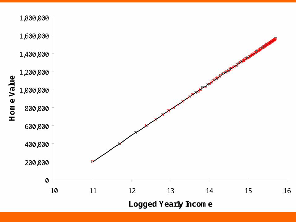
Income and home value

• $60,000/year $200,000 home

• $120,000/year $400,000 home

• Bill Gates makes about $175 million/year– $175,000,000 = 2917 x $60,000 – Should we expect him to have a 2917 x

$200,000 ($583,400,000) home?

0

200,000

400,000

600,000

800,000

1,000,000

1,200,000

1,400,000

1,600,000

1,800,000

60,0

00

660,

000

1,26

0,00

0

1,86

0,00

0

2,46

0,00

0

3,06

0,00

0

3,66

0,00

0

4,26

0,00

0

4,86

0,00

0

5,46

0,00

0

6,06

0,00

0

6,66

0,00

0

Yearly Income ($s)

Ho

me

Va

lue

($

s)

0

200,000

400,000

600,000

800,000

1,000,000

1,200,000

1,400,000

1,600,000

1,800,000

10 11 12 13 14 15 16

Logged Yearly Income

Ho

me

Va

lue

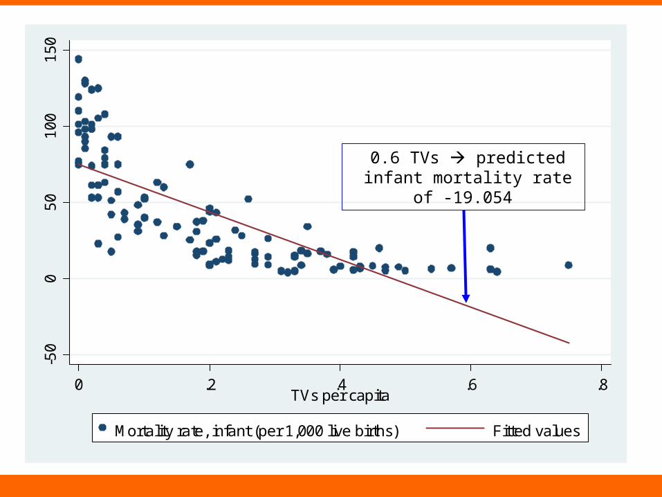
TVs and Infant Mortality

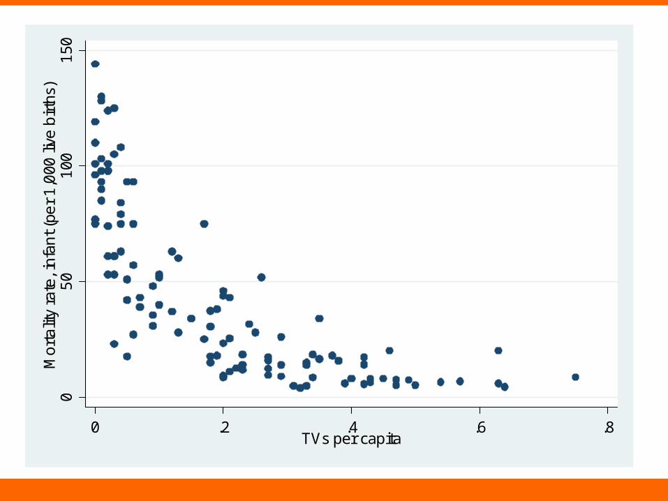
• TVs as proxy for resources or wealth

• Biggest differences at the low end?– E.g., “there are a couple of TVs in town” and

“some people have TVs in their private homes”

05

01

001

50M

ort

alit

y ra

te, i

nfan

t (pe

r 1

,000

live

birt

hs)

0 .2 .4 .6 .8TVs per capita

-50

05

01

001

50

0 .2 .4 .6 .8TVs per capita

Mortality rate, infant (per 1,000 live births) Fitted values

0.6 TVs predicted infant mortality rate of -19.054

Coef. SE T P

TVs per capita -156.436 12.934 -12.100 0.000

Constant 74.810 3.419 21.880 0.000

Coef. SE T P

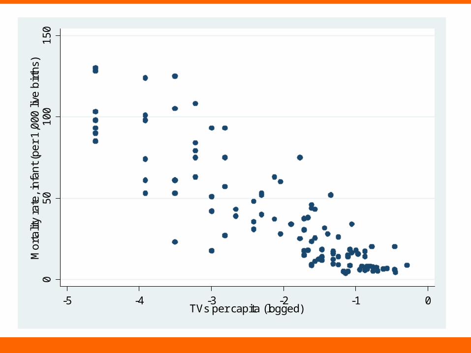
TVs per capita (logged) -24.656 1.397 -17.640 0.000

Constant -11.151 3.346 -3.330 0.001

R-squared = 0.566

R-squared = 0.748

05

01

001

50M

ort

alit

y ra

te, i

nfan

t (pe

r 1

,000

live

birt

hs)

-5 -4 -3 -2 -1 0TVs per capita (logged)

05

01

001

50

-5 -4 -3 -2 -1 0TVs per capita (logged)

Mortality rate, infant (per 1,000 live births) Fitted values

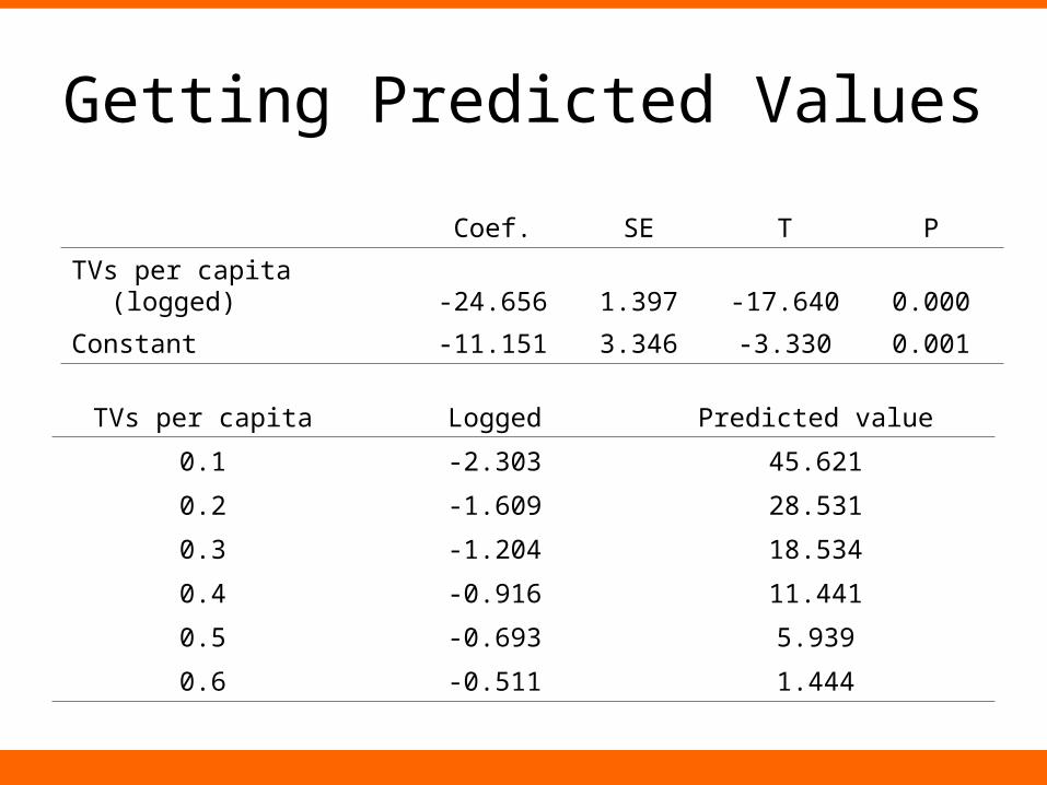
Getting Predicted Values

Coef. SE T P

TVs per capita (logged) -24.656 1.397 -17.640 0.000

Constant -11.151 3.346 -3.330 0.001

TVs per capita Logged Predicted value

0.1 -2.303 45.621

0.2 -1.609 28.531

0.3 -1.204 18.534

0.4 -0.916 11.441

0.5 -0.693 5.939

0.6 -0.511 1.444

05

01

001

50

0 .2 .4 .6 .8TVs per capita

Mortality rate, infant (per 1,000 live births) pred_value

Quadratic (squared) models

• Curved like logarithm– Key difference: quadratics allow for

“U-shaped” relationship

• Enter original variable and squared term– Allows for a direct test of whether allowing the

line to curve significantly improves the predictive power of the model

-500

0

500

1000

1500

2000

2500

3000

0 5 10 15 20 25 30 35 40 45 50

Original Value

Tra

nsf

orm

ed V

alu

e

Original+Squared

Original+.5*Squared

-10*Original+0.3*Squared

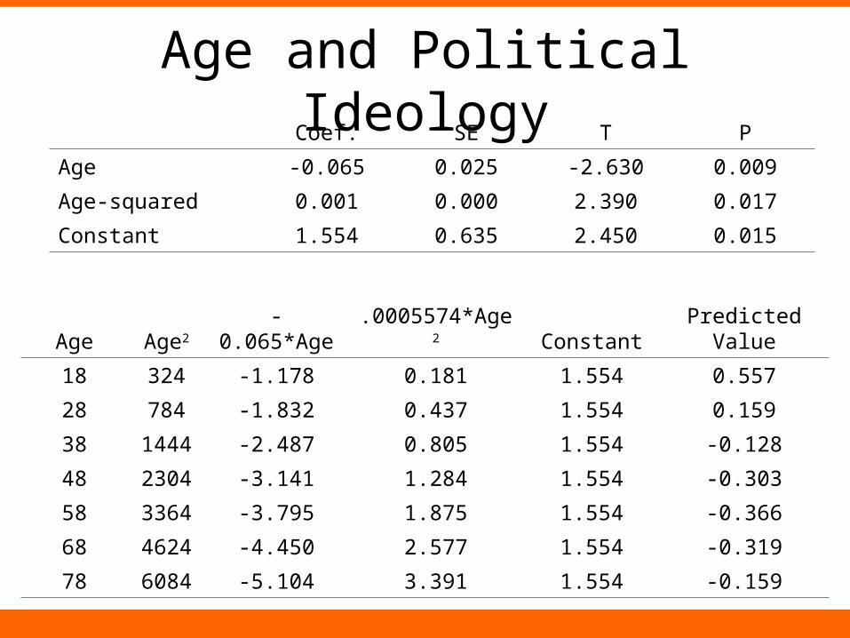
Age and Political Ideology

Coef. SE T P

Age -0.007 0.004 -1.740 0.082

Constant 0.122 0.209 0.580 0.561

Coef. SE T P

Age -0.065 0.025 -2.630 0.009

Age-squared 0.001 0.000 2.390 0.017

Constant 1.554 0.635 2.450 0.015

What would we conclude from this analysis?

Age and Political IdeologyCoef. SE T P

Age -0.065 0.025 -2.630 0.009

Age-squared 0.001 0.000 2.390 0.017

Constant 1.554 0.635 2.450 0.015

Age Age2 -0.065*Age .0005574*Age2 Constant Predicted Value

18 324 -1.178 0.181 1.554 0.557

28 784 -1.832 0.437 1.554 0.159

38 1444 -2.487 0.805 1.554 -0.128

48 2304 -3.141 1.284 1.554 -0.303

58 3364 -3.795 1.875 1.554 -0.366

68 4624 -4.450 2.577 1.554 -0.319

78 6084 -5.104 3.391 1.554 -0.159

-1

-0.5

0

0.5

1

18 28 38 48 58 68 78 88

Age

Ide

olo

gy

(-

2=

ve

ry c

on

se

rva

tiv

e, 2

=v

ery

lib

era

l)

Age and Political IdeologyCoef. SE T P

Age -0.065 0.025 -2.630 0.009

Age-squared 0.001 0.000 2.390 0.017

Constant 1.554 0.635 2.450 0.015

Note: We are using two variables to measure the relationship between age and ideology.

Interpretation: 1. statistically significant relationship between age and ideology

(can confirm with an F-test)2. squared term significantly contributes to the predictive power

of the model.

If you add a linear and squared term (e.g., age and age2) to a model and neither is

independently statistically significant

• This does not necessarily mean that age is not significantly related to the outcome Why?

• What we want to know is whether age and age2 jointly improve the predictive power of the model. How can we test this?

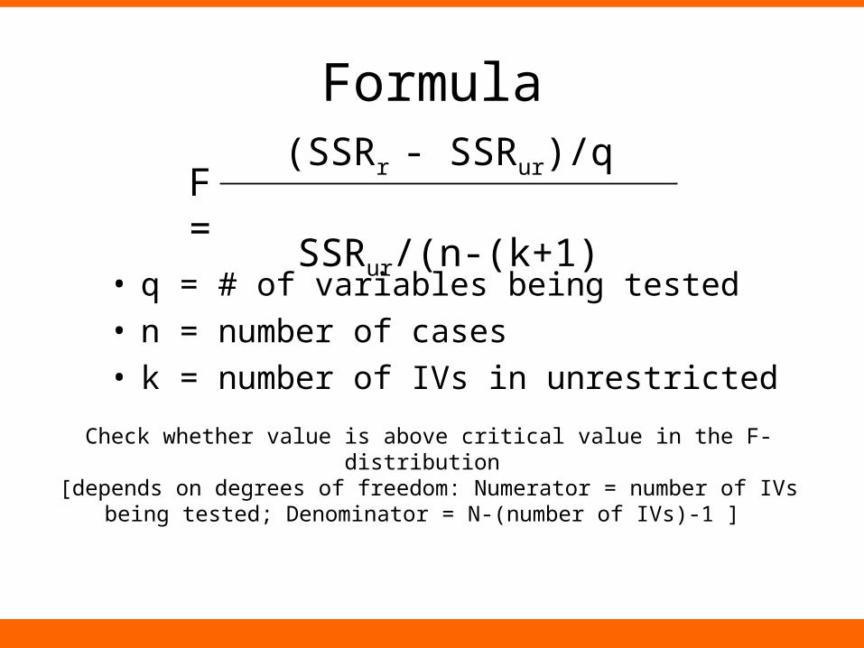
Formula

• q = # of variables being tested• n = number of cases• k = number of IVs in unrestricted

F =(SSRr - SSRur)/q

SSRur/(n-(k+1)

Check whether value is above critical value in the F-distribution [depends on degrees of freedom: Numerator = number of IVs being tested;

Denominator = N-(number of IVs)-1 ]

Don’t worry about the F-test formula

• The point is:– F-tests are a way to test whether adding a set

of variables reduces the sum of squared residuals enough to justify throwing these new variables into the model

• Depends on:– How much sum of squared residuals is reduced– How many variables we’re adding– How many cases we have to work with

• More “acceptable” to add variables if you have a lot of cases

• Intuition: explaining 10 cases with 10 variables v. explaining 1000 cases with 10 variables?

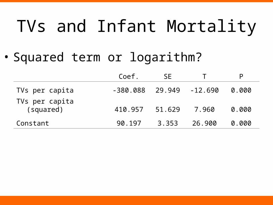
TVs and Infant Mortality

• Squared term or logarithm?

Coef. SE T P

TVs per capita -380.088 29.949 -12.690 0.000

TVs per capita (squared) 410.957 51.629 7.960 0.000

Constant 90.197 3.353 26.900 0.000

05

01

001

50

0 .2 .4 .6 .8

Which is “better”?

Two basic ways to decide: 1) Theory2) Which yields a better fit?

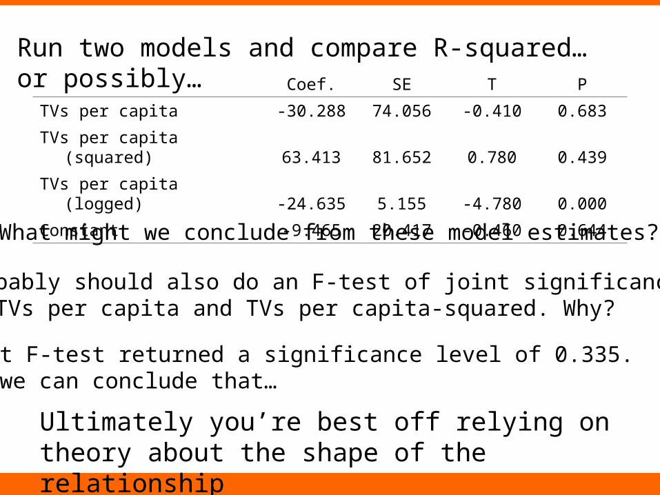
Coef. SE T P

TVs per capita -30.288 74.056 -0.410 0.683

TVs per capita (squared) 63.413 81.652 0.780 0.439

TVs per capita (logged) -24.635 5.155 -4.780 0.000

Constant -9.465 20.417 -0.460 0.644

What might we conclude from these model estimates?

Probably should also do an F-test of joint significance of TVs per capita and TVs per capita-squared. Why?

That F-test returned a significance level of 0.335. So we can conclude that…

Run two models and compare R-squared… or possibly…

Ultimately you’re best off relying on theory about the shape of the relationship

Ordered IVs Indicators

• Sometimes we have reason to expect the relationship between an IV and outcome to be more complex

• Can address this using more polynomials (e.g., variable3, variable4, etc) – We won’t go there… instead…

• Example: Party identification and evaluations of candidates and issues

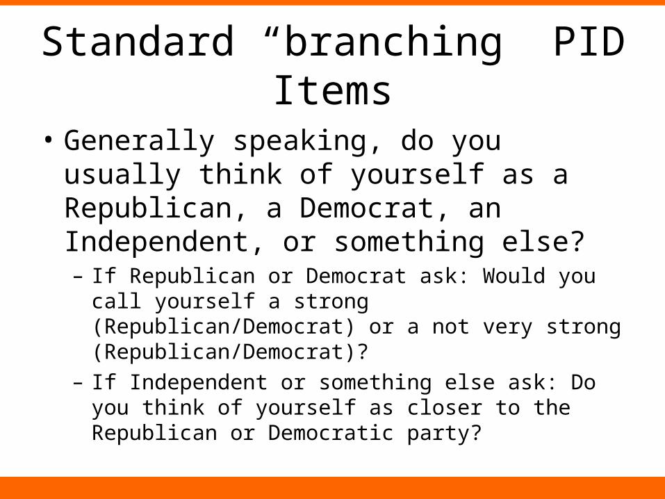
Standard “branching” PID Items

• Generally speaking, do you usually think of yourself as a Republican, a Democrat, an Independent, or something else? – If Republican or Democrat ask: Would you call

yourself a strong (Republican/Democrat) or a not very strong (Republican/Democrat)?

– If Independent or something else ask: Do you think of yourself as closer to the Republican or Democratic party?

Party Identification Measure

Strong Republican

Weak Republican

Lean Republican Independent

Lean Democrat

Weak Democrat

Strong Democrat

-3 -2 -1 0 1 2 3

People who say Democrat or Republican in response to first question

Question: Is the change from -2 to -1 (or 1 to 2) the same as the change from 0 to 1 or 2 to 3?

Create Indicators

Party Identification (-3 to 3)

Seven Variables:Strong Republican (1=yes) Weak Republican (1=yes) Lean Republican (1=yes) Pure Independent (1=yes) Lean Democrat (1=yes) Weak Democrat (1=yes) Strong Democrat (1=yes)

Predict Obama Favorability (1-4)

Coef. SE T P

Strong Republican -1.632 0.161 -10.160 0.000

Weak Republican -0.707 0.198 -3.580 0.000

Lean Republican -1.235 0.181 -6.810 0.000

Lean Democrat 0.674 0.197 3.430 0.001

Weak Democrat 0.494 0.187 2.640 0.009

Strong Democrat 0.595 0.159 3.750 0.000

Constant 2.940 0.134 21.870 0.000

Excluded category: Pure Independents

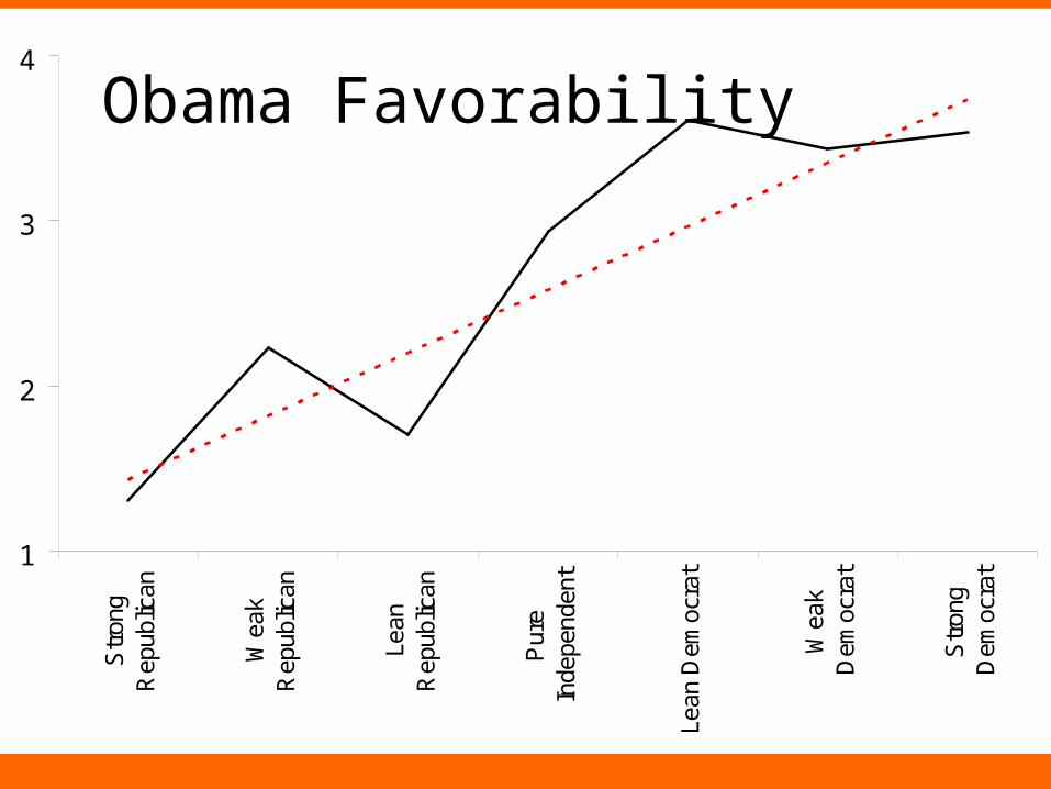
1

2

3

4

Str

ong

Rep

ublic

an

Wea

kR

epub

lican

Lean

Rep

ublic

an

Pur

eIn

depe

nden

t

Lean

Dem

ocra

t

Wea

kD

emoc

rat

Str

ong

Dem

ocra

t

Obama Favorability

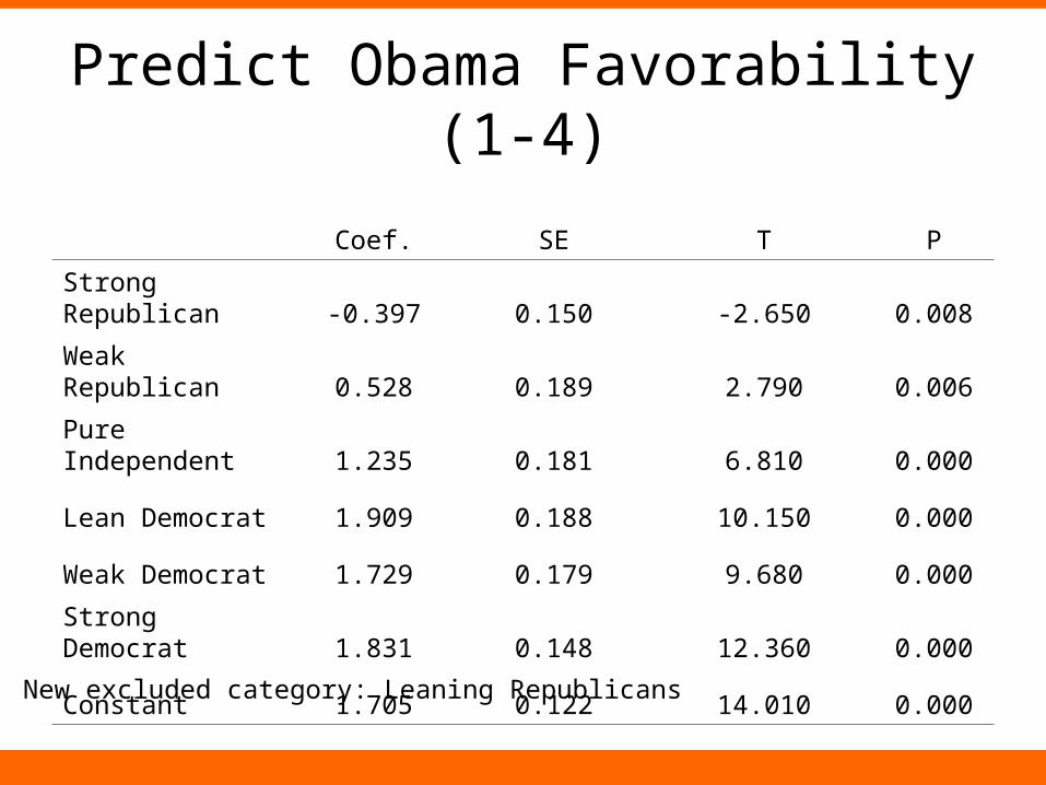
Predict Obama Favorability (1-4)

Coef. SE T P

Strong Republican -0.397 0.150 -2.650 0.008

Weak Republican 0.528 0.189 2.790 0.006

Pure Independent 1.235 0.181 6.810 0.000

Lean Democrat 1.909 0.188 10.150 0.000

Weak Democrat 1.729 0.179 9.680 0.000

Strong Democrat 1.831 0.148 12.360 0.000

Constant 1.705 0.122 14.010 0.000

New excluded category: Leaning Republicans

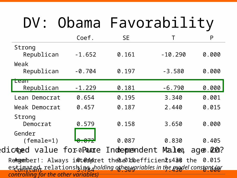
DV: Obama FavorabilityCoef. SE T P

Strong Republican -1.652 0.161 -10.290 0.000

Weak Republican -0.704 0.197 -3.580 0.000

Lean Republican -1.229 0.181 -6.790 0.000

Lean Democrat 0.654 0.195 3.340 0.001

Weak Democrat 0.457 0.187 2.440 0.015

Strong Democrat 0.579 0.158 3.650 0.000

Gender (female=1) 0.072 0.087 0.830 0.405

Age -0.041 0.019 -2.140 0.033

Age2 0.044 0.018 2.430 0.015

Constant 3.784 0.509 7.430 0.000

Predicted value for Pure Independent Male, age 20?Remember!: Always interpret these coefficients as the estimated relationships holding other variables in the model constant (or controlling for the other variables)

Notes and Next Time

• Homework due next Thursday (11/18)

• Next homework handed out next Tuesday– Not due until Tuesday after Fall Break

• Next time: – Dealing with situations where you expect the

relationship between an IV and a DV to depend on the value of another IV