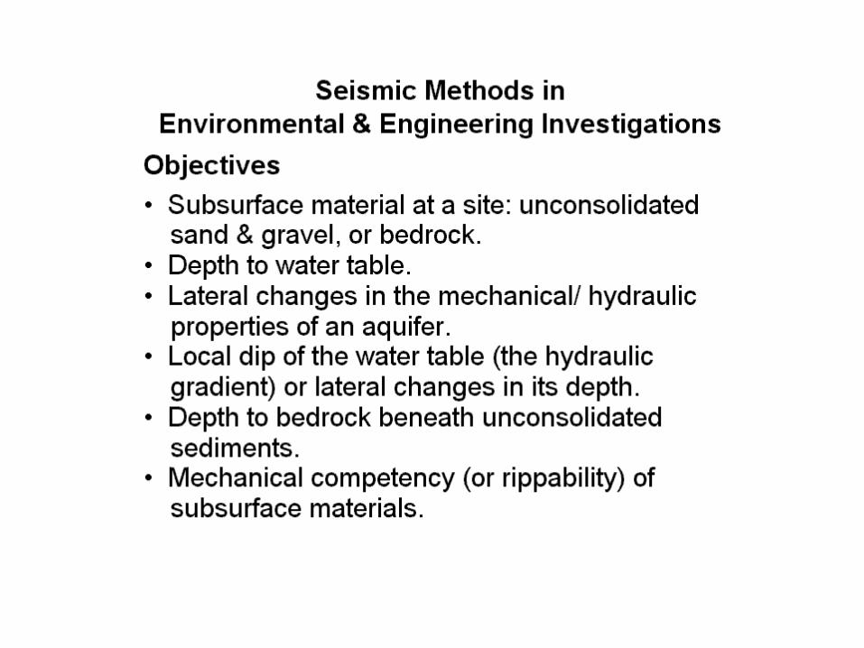
introduction to seismic method
TRANSCRIPT

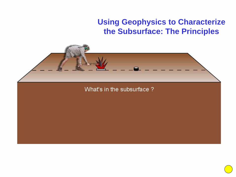
Using Geophysics to Characterize
the Subsurface:
“The Principles”
BERAN GÜRLEME
OCAK/2011
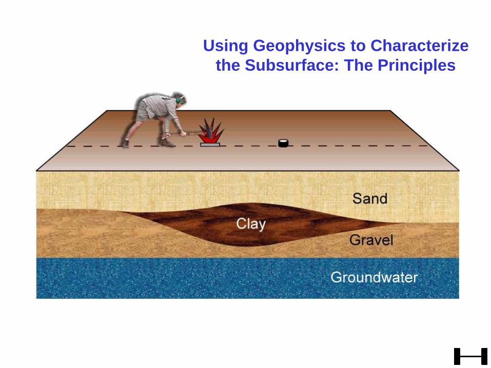
Using Geophysics to Characterize
the Subsurface: The Principles
Using Geophysics to Characterize
the Subsurface: The Principles

We determine subsurface conditions by remotely sensing physical
properties of materials in situ.
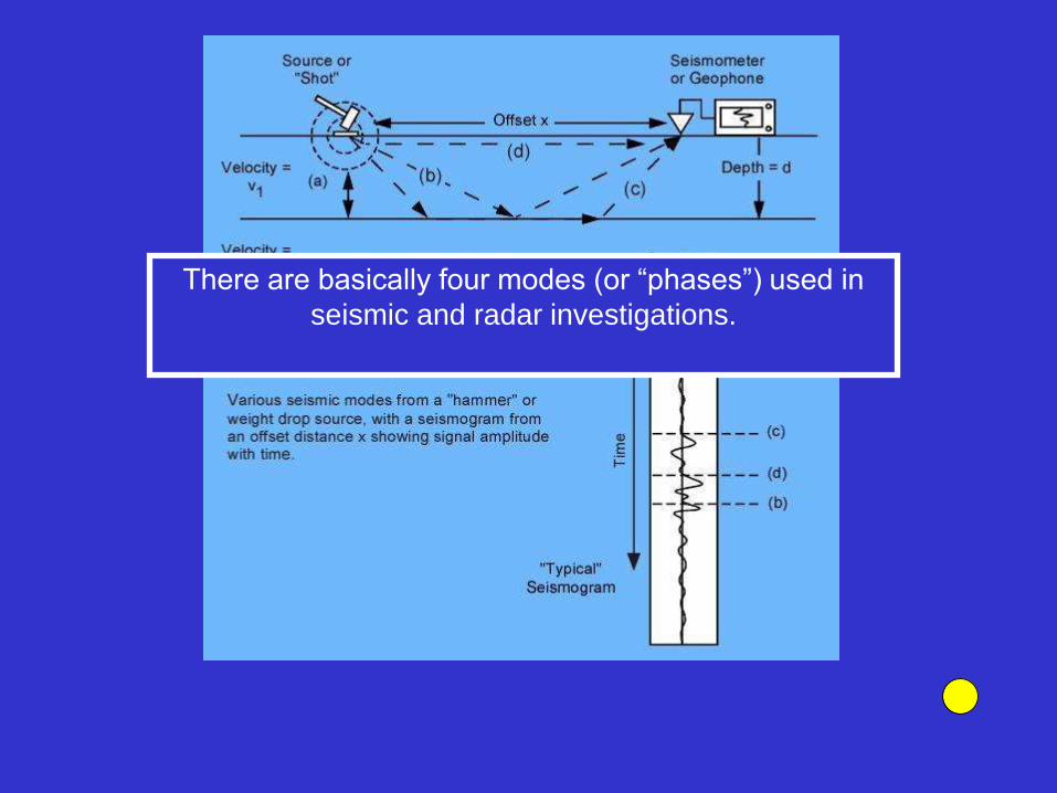
There are basically four modes (or “phases”) used in
seismic and radar investigations.
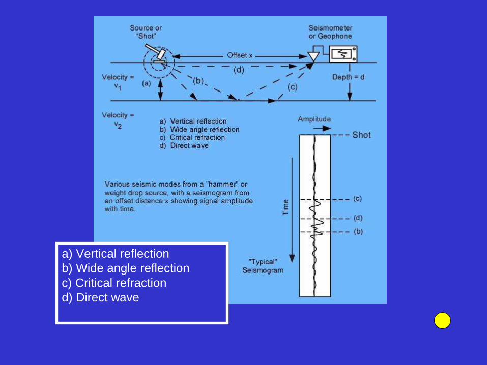
a) Vertical reflection
b) Wide angle reflection
c) Critical refraction
d) Direct wave
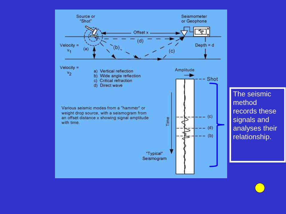
The seismic
method
records these
signals and
analyses their
relationship.

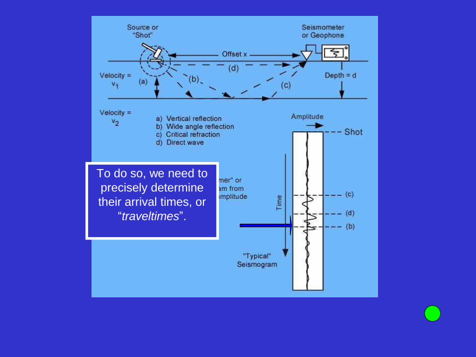
To do so, we need to
precisely determine
their arrival times, or
“traveltimes”.

To do so, we need to
precisely determine
their arrival times, or
“traveltimes”.
To do so, we need to
precisely determine
their arrival times, or
“traveltimes”.
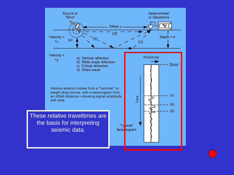
These relative traveltimes are
the basis for interpreting
seismic data.
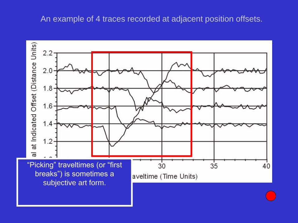
“Picking” traveltimes (or “first
breaks”) is sometimes a
subjective art form.
An example of 4 traces recorded at adjacent position offsets.
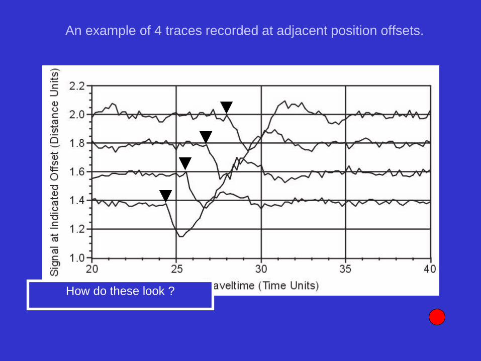
How do these look ?
An example of 4 traces recorded at adjacent position offsets.
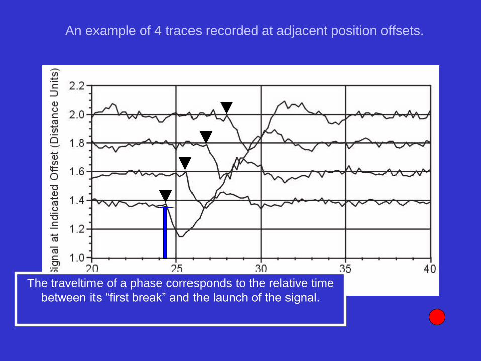
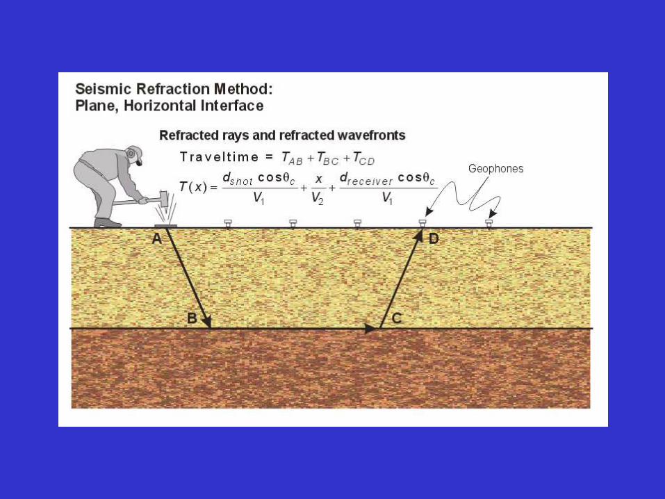
The traveltime of a phase corresponds to the relative time
between its “first break” and the launch of the signal.
An example of 4 traces recorded at adjacent position offsets.
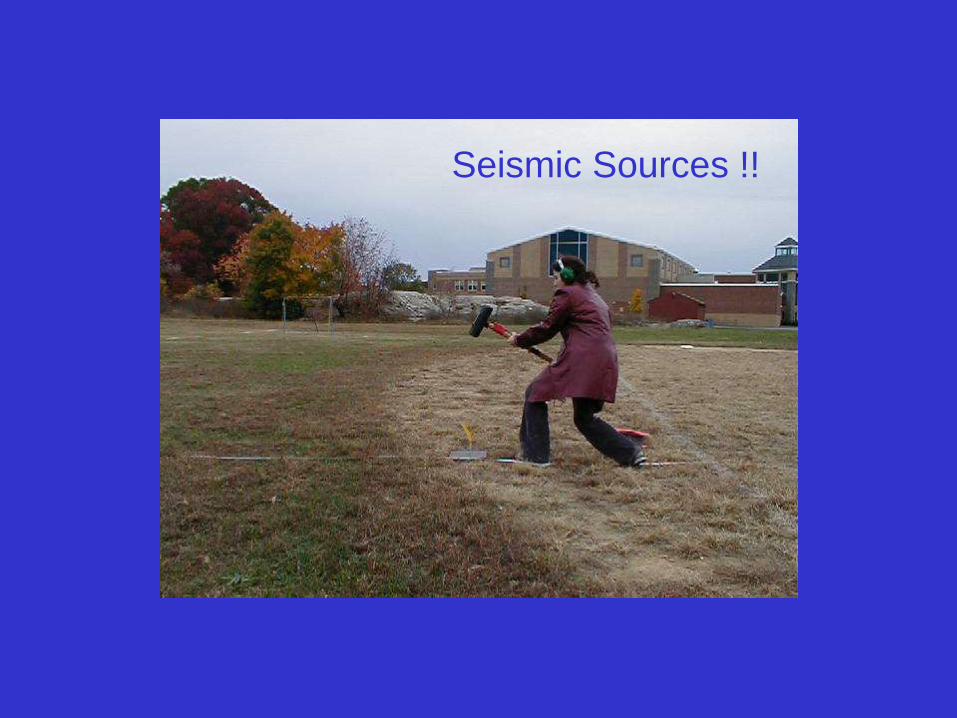
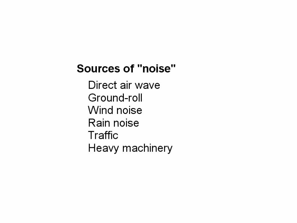
Seismic Sources !!
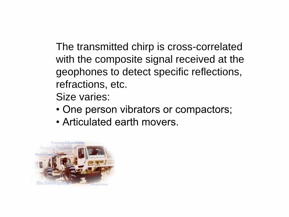
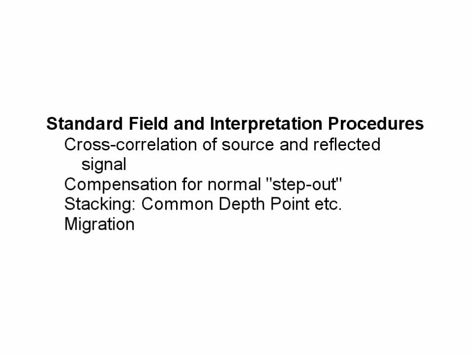
The transmitted chirp is cross-correlated
with the composite signal received at the
geophones to detect specific reflections,
refractions, etc.
Size varies:
• One person vibrators or compactors;
• Articulated earth movers.

(U British Columbia:
Lithoprobe Project.)(University of Bergen.)
(Network for Earthquake Engineering
Simulation; U Texas.)

Vibrating type sources

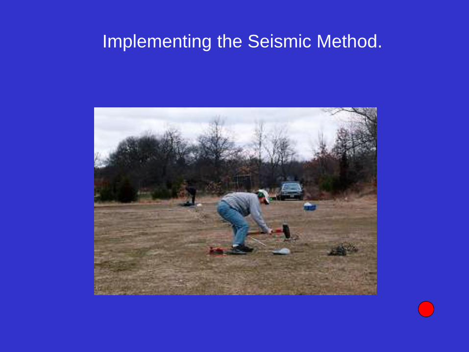
Implementing the Seismic Method.
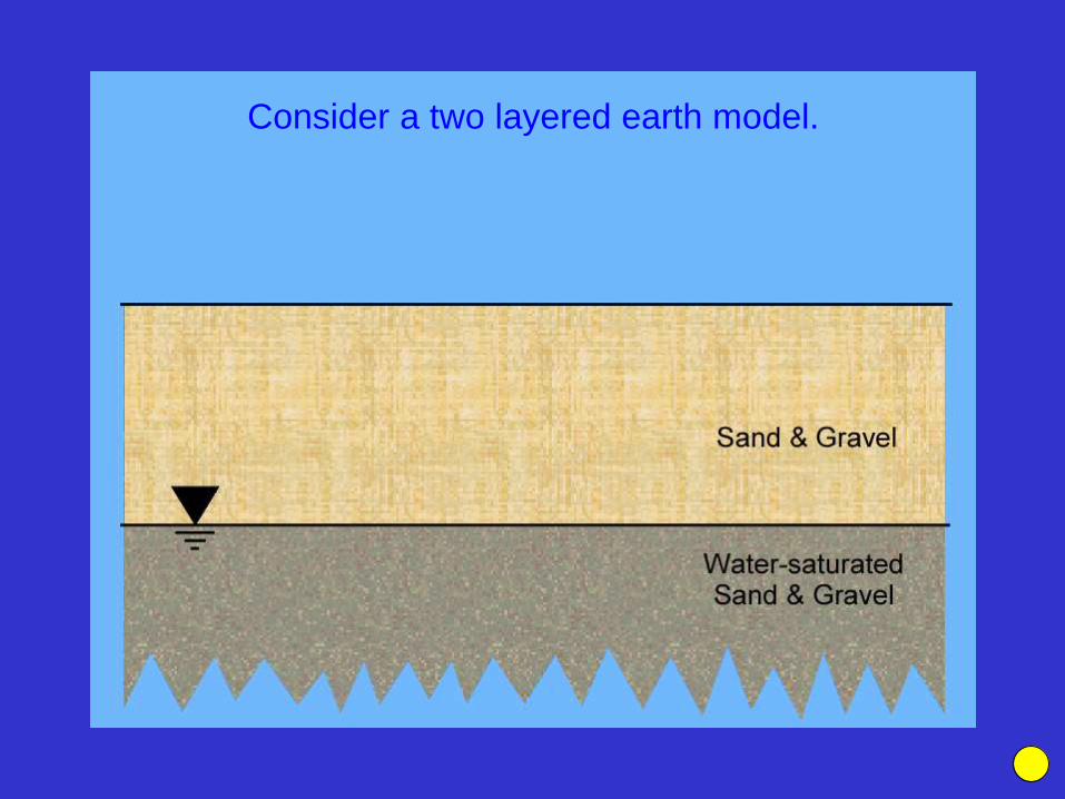
Consider a two layered earth model.
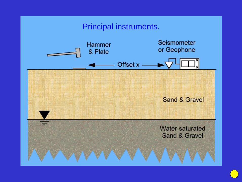
Principal instruments.
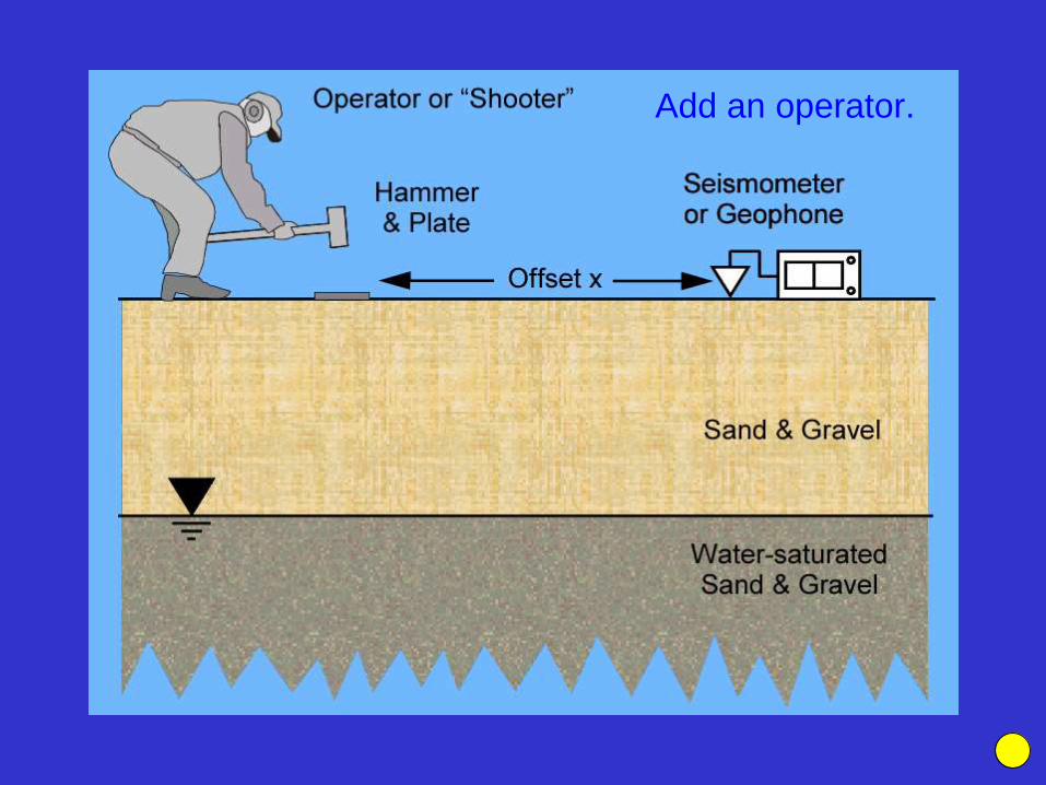
Add an operator.
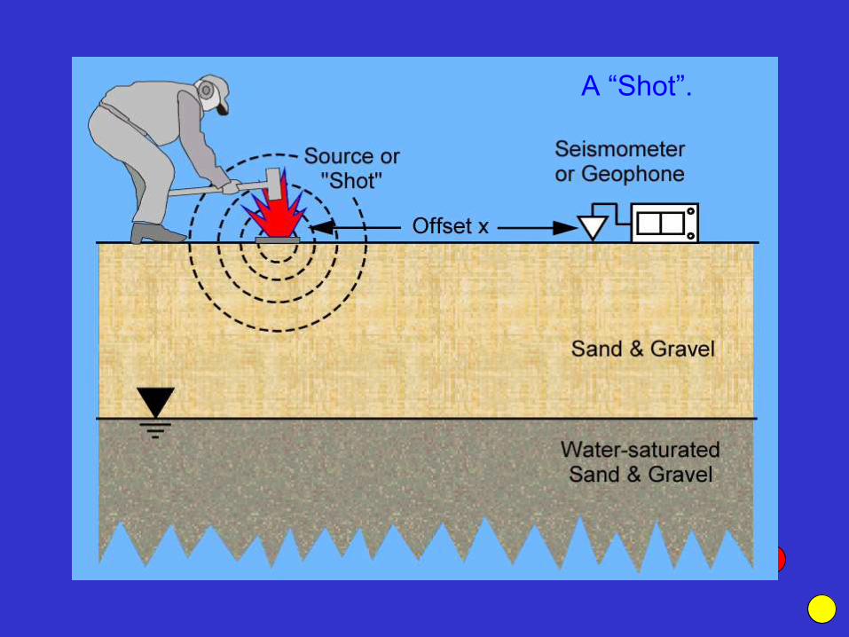
A “Shot”.

A sound pulse is generated.

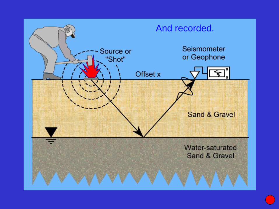
And recorded.

And . . .

. . . a reflection is generated.
And recorded.
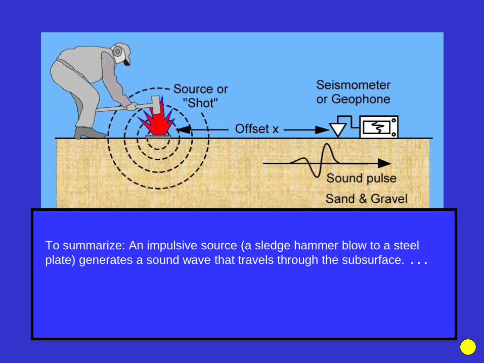
To summarize: An impulsive source (a sledge hammer blow to a steel
plate) generates a sound wave that travels through the subsurface. . . .
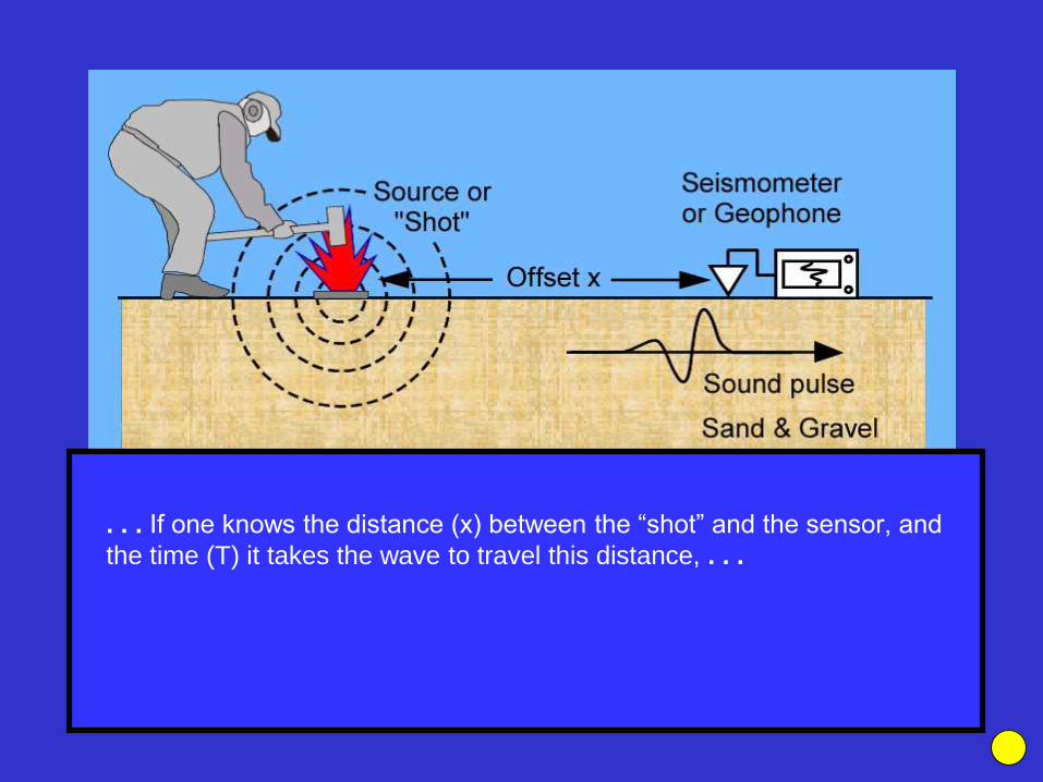
. . . If one knows the distance (x) between the “shot” and the sensor, and
the time (T) it takes the wave to travel this distance, . . .
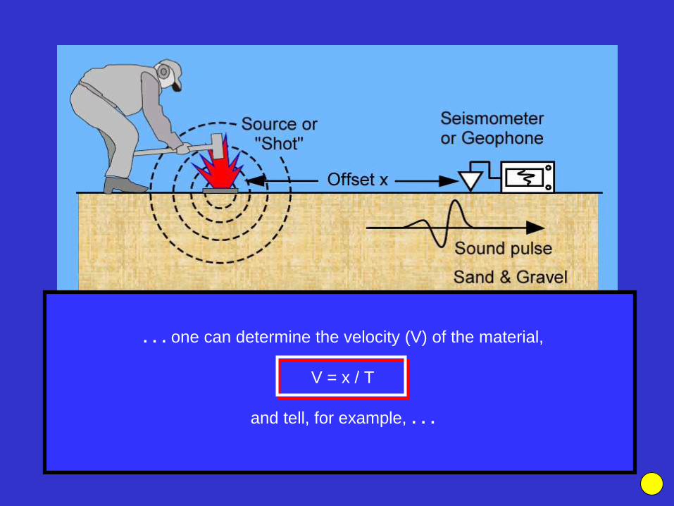
. . . one can determine the velocity (V) of the material,
V = x / T
and tell, for example, . . .
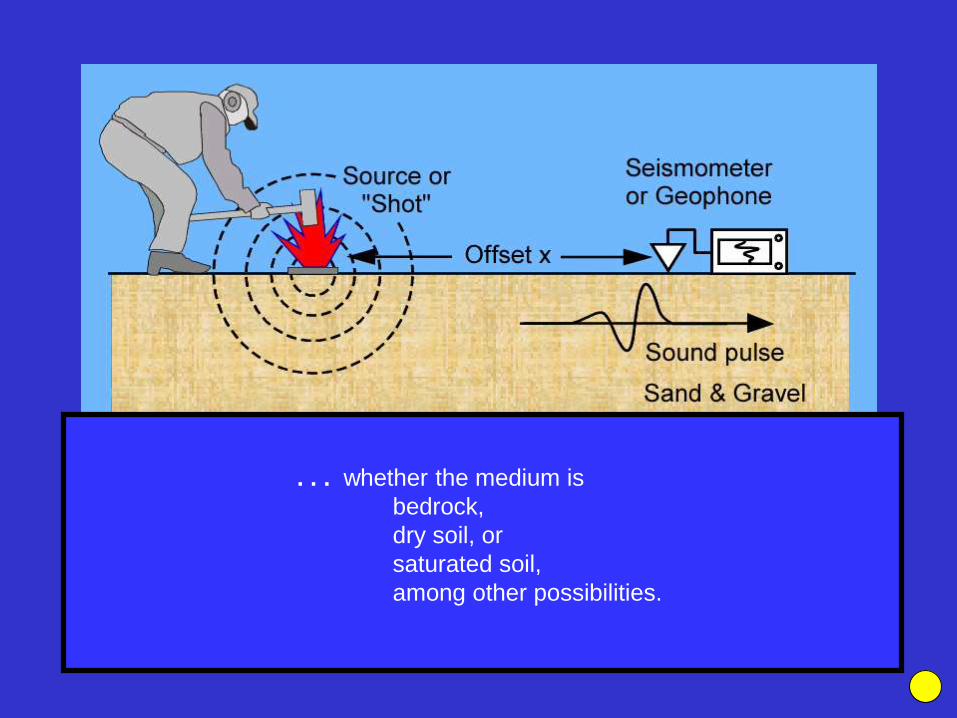
. . . whether the medium is
bedrock,
dry soil, or
saturated soil,
among other possibilities.
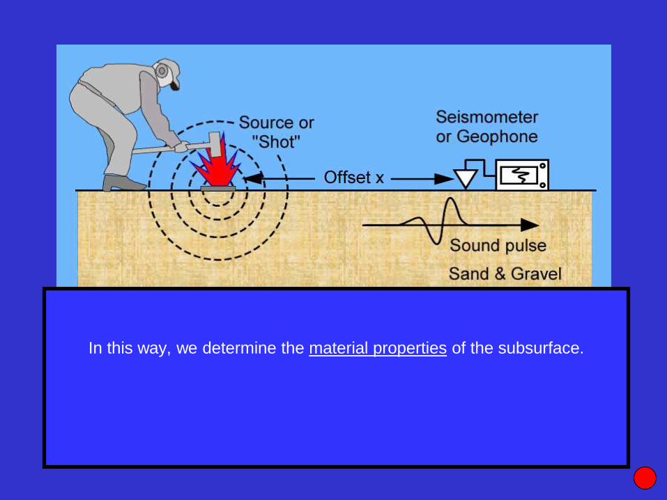
In this way, we determine the material properties of the subsurface.

Alternatively, if one knows the velocity (V) of the material and the
time (T) it takes the wave to get to a sensor, then rearranging
V = x / T
. . .
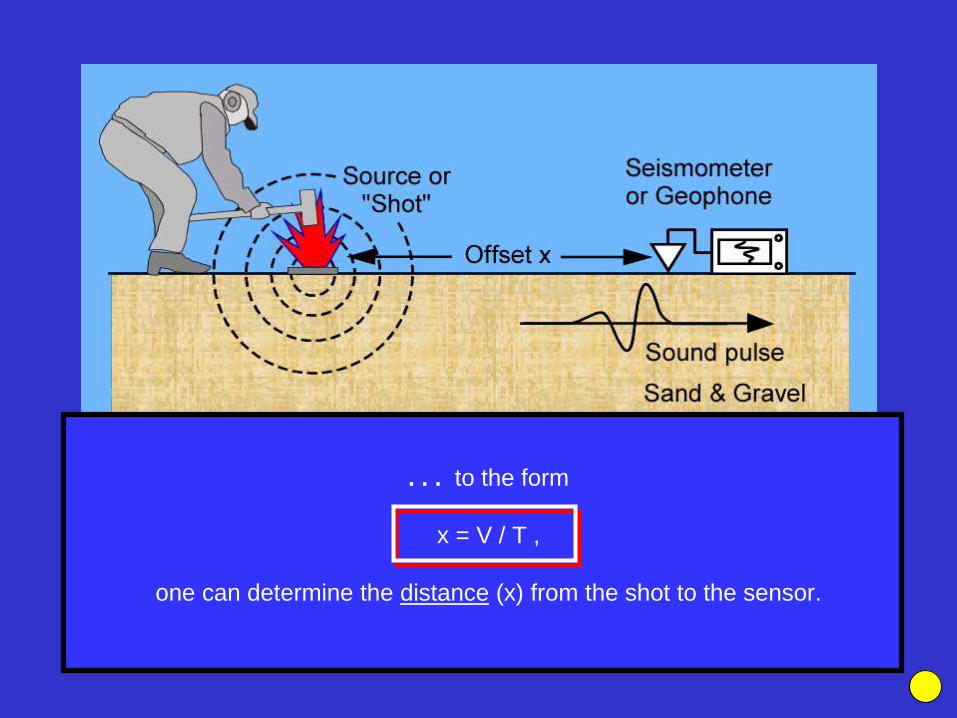
. . . to the form
x = V / T ,
one can determine the distance (x) from the shot to the sensor.
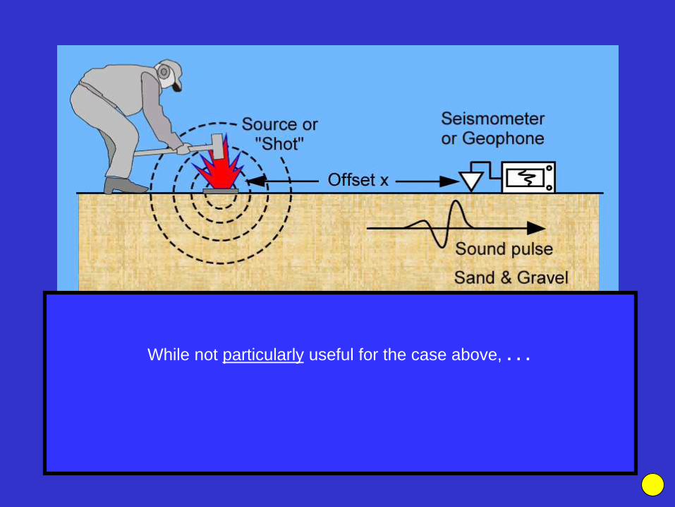
While not particularly useful for the case above, . . .
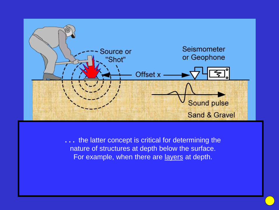
. . . the latter concept is critical for determining the
nature of structures at depth below the surface.
For example, when there are layers at depth.

Determining the depth when V and T are known is the
principle of the reflection method.
Theory: Behavior of Waves in the Subsurface
In order to understand how to extract more detailed
subsurface information from geophysical measurements at the
surface, we first analyze the behavior of waves (seismic or
radar) in the subsurface.
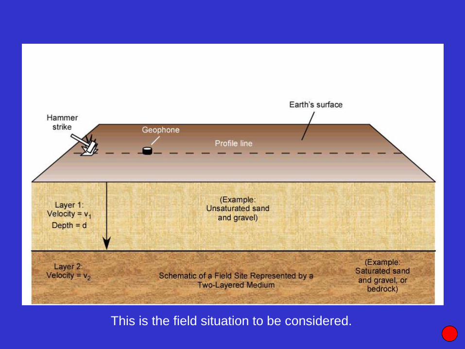
This is the field situation to be considered.
Please review the animation sequence for
Reflected Phases at this time.
Please minimize this application, the animation
sequence is found on the index page.
Maximize this application when ready to continue.
Essential points for discussion.
1) The relative difference in arrival times of the ‘direct’ and
‘reflected’ phases as offset increases.
Essential points for discussion.
1) The relative difference in arrival times of the ‘direct’ and
‘reflected’ phases as offset increases.
2) The synchrony of the two phases along the lower
interface.
Essential points for discussion.
1) The relative difference in arrival times of the ‘direct’ and
‘reflected’ phases as offset increases.
2) The synchrony of the two phases along the lower
interface.
3) The difference in the ‘apparent’ velocity of the two
phases along the surface
a) The direct (primary) wave travels @ v1.
b) The reflected wave @ v1 / sin θ i(where θ i is the incident angle).

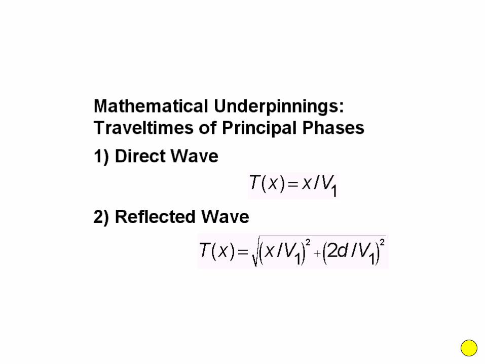
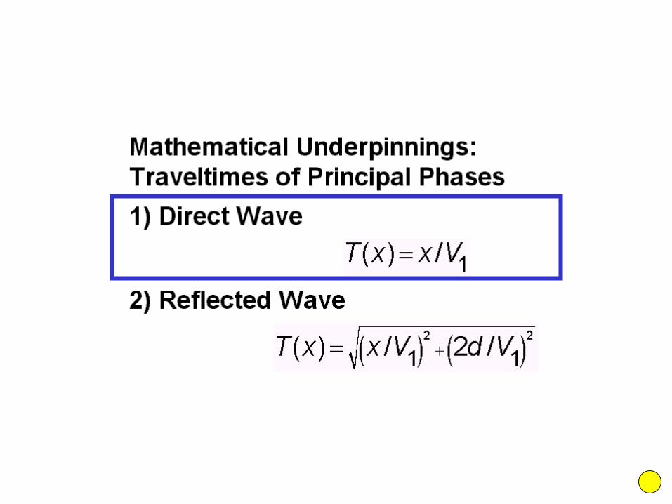
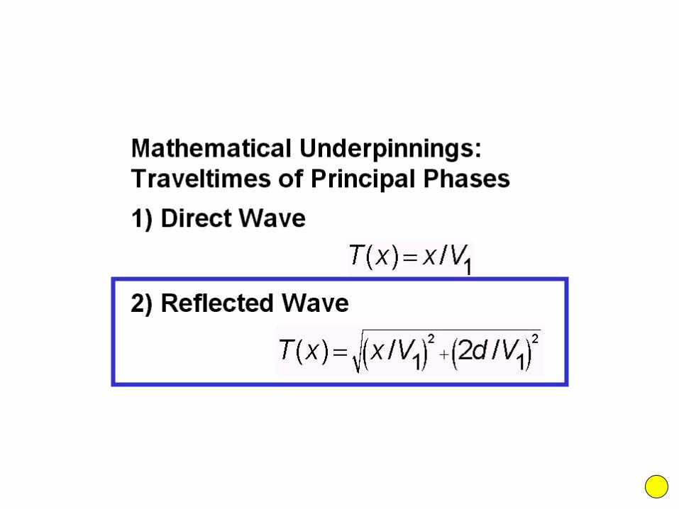
Traveltime Relations for Direct and
Reflected Phases
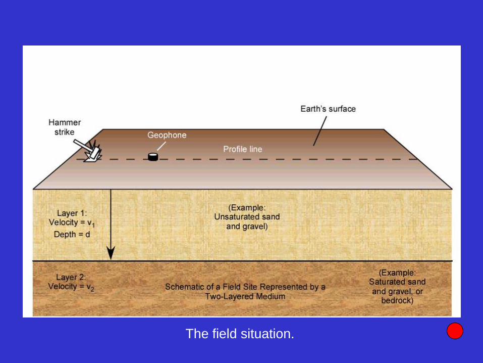
The field situation.
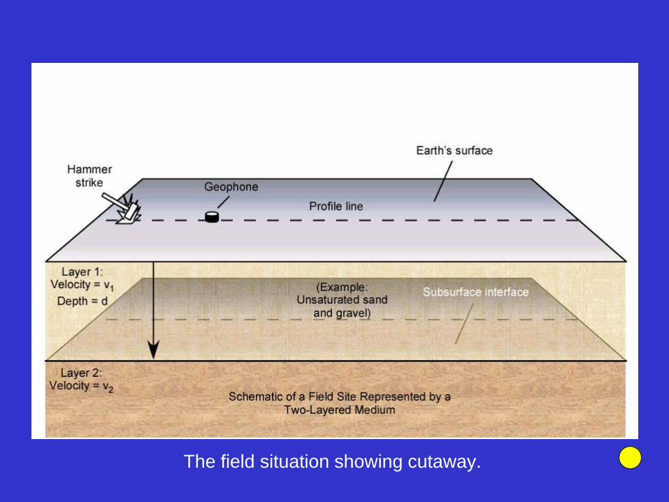
The field situation showing cutaway.
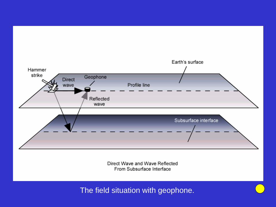
The field situation with geophone.

Direct and reflected ray paths.
How can we use the ‘reflected’ phase to
determine the depth to the respective
horizon (or layer) ?
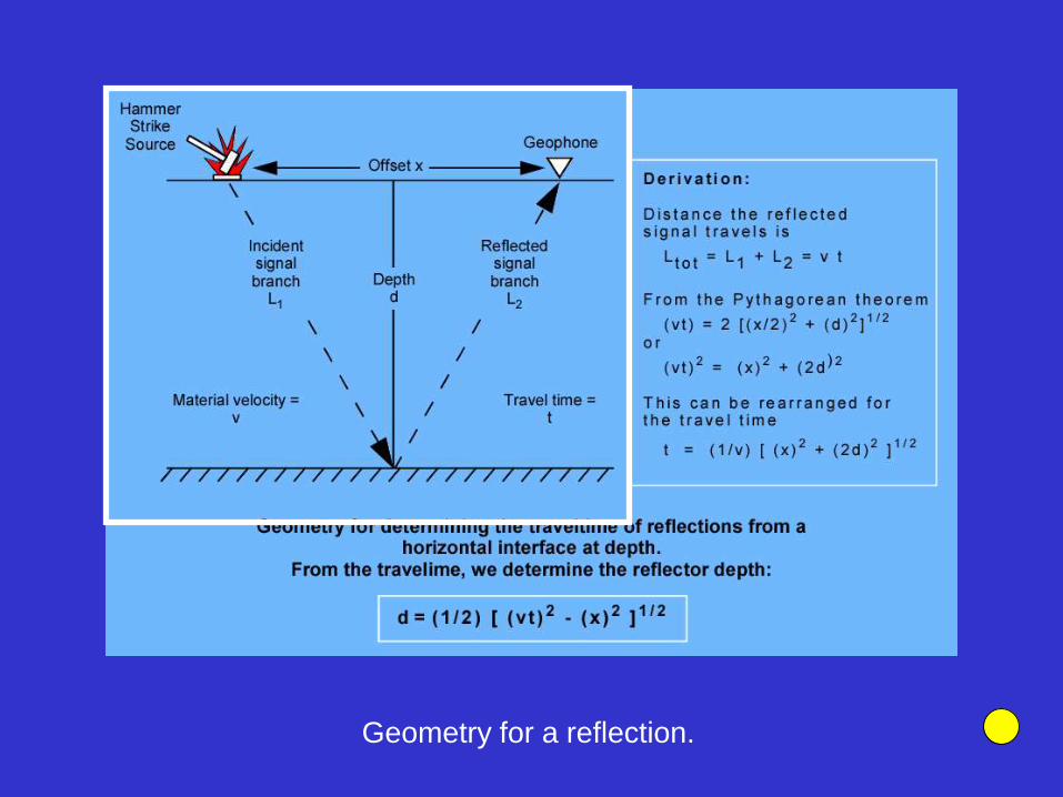
Geometry for a reflection.
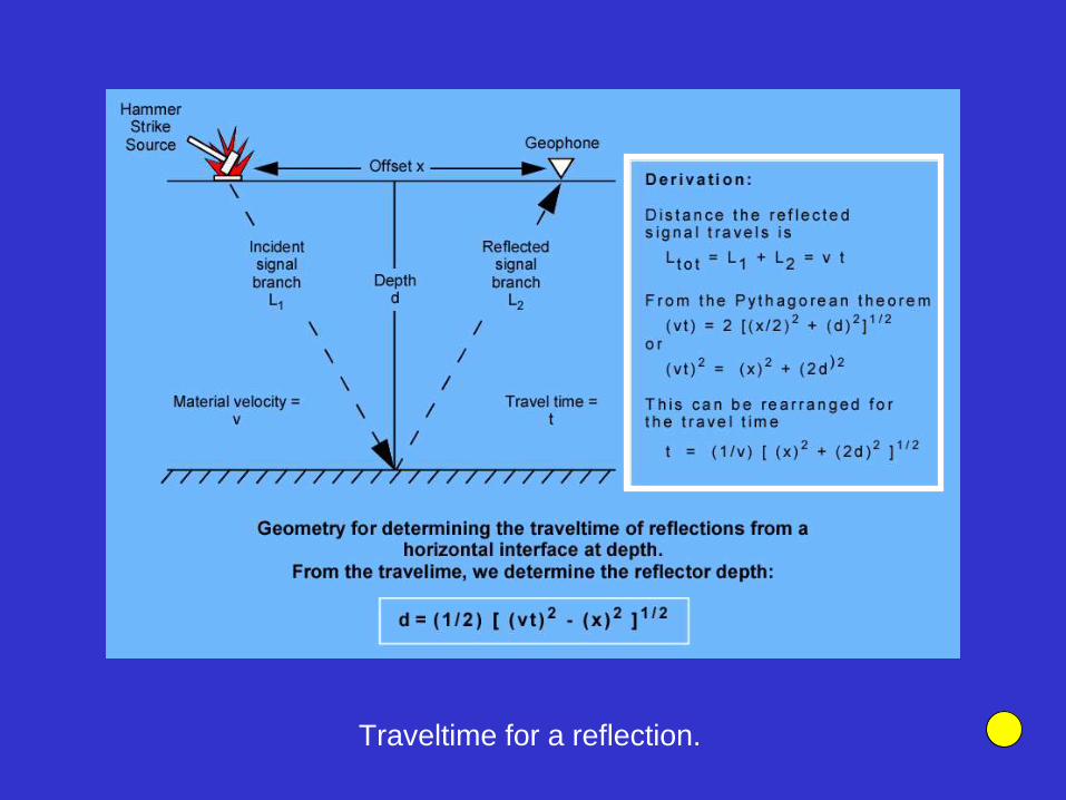
Traveltime for a reflection.
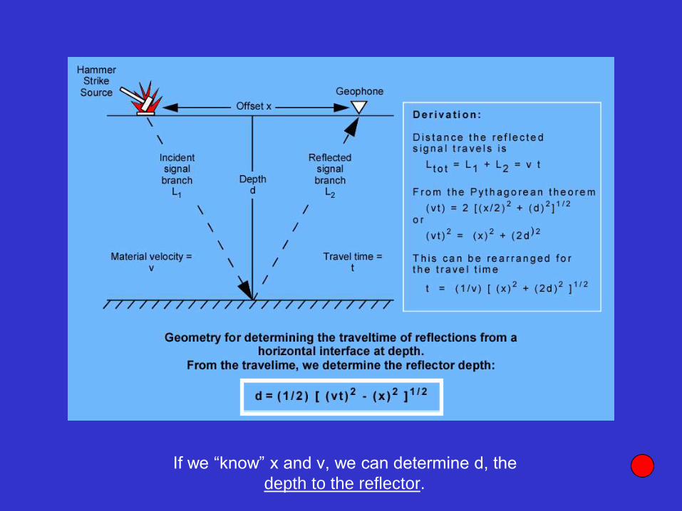
If we “know” x and v, we can determine d, the
depth to the reflector.

Direct and reflected ray paths with traveltimes.
Please review tutorial on Analyzing Direct and
Reflected Phases at this time.
Please minimize this application, the tutorial is
found on the index page.
Maximize this application when ready to continue.

Next, consider the ‘refracted’ phase.
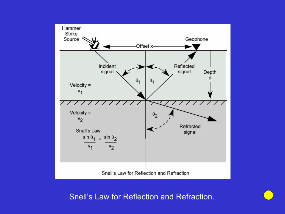
Snell’s Law for Reflection and Refraction.

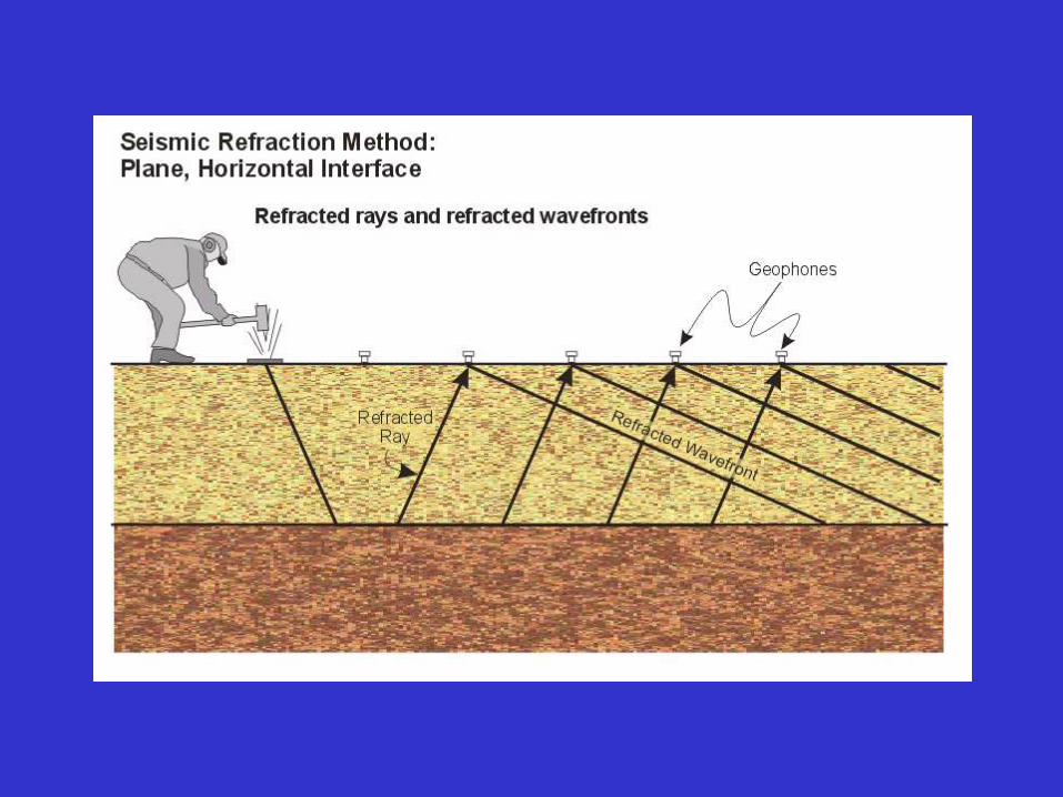
Refraction at the Critical Angle.
Please review the animation sequence for
Refracted Phases at this time.
Please minimize this application, the animation
sequence is found on the index page.
Maximize this application when ready to continue.

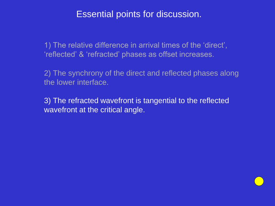
Essential points for discussion.
1) The relative difference in arrival times of the ‘direct’,
‘reflected’ & ‘refracted’ phases as offset increases.
Essential points for discussion.
1) The relative difference in arrival times of the ‘direct’,
‘reflected’ & ‘refracted’ phases as offset increases.
2) The synchrony of the direct and reflected phases along
the lower interface.
Essential points for discussion.
1) The relative difference in arrival times of the ‘direct’,
‘reflected’ & ‘refracted’ phases as offset increases.
2) The synchrony of the direct and reflected phases along
the lower interface.
3) The refracted wavefront is tangential to the reflected
wavefront at the critical angle.

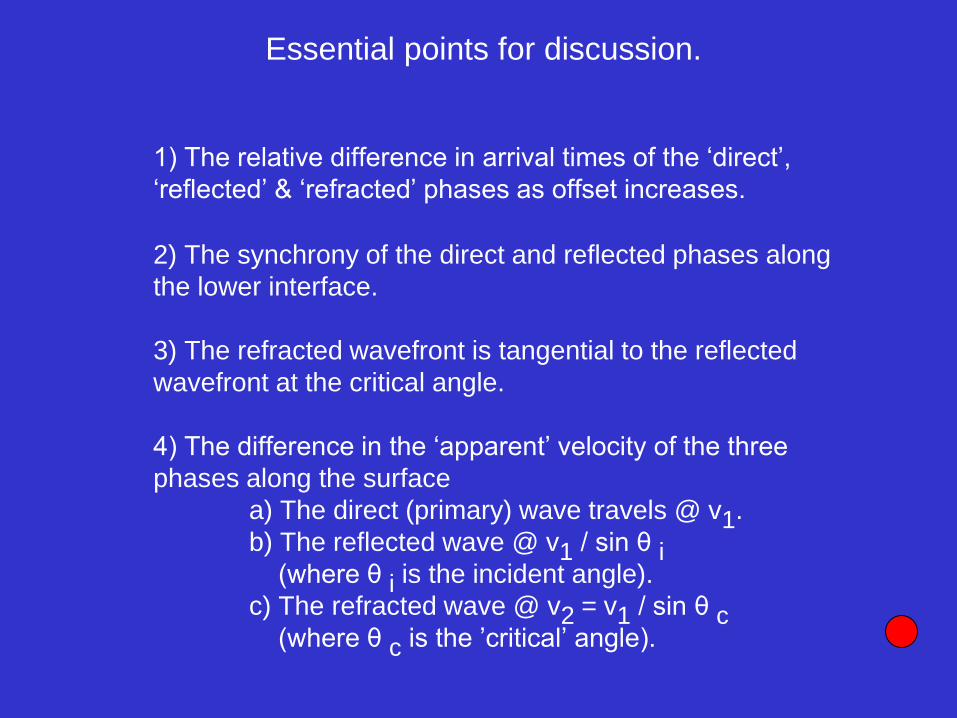
Essential points for discussion.
1) The relative difference in arrival times of the ‘direct’,
‘reflected’ & ‘refracted’ phases as offset increases.
2) The synchrony of the direct and reflected phases along
the lower interface.
4) The difference in the ‘apparent’ velocity of the three
phases along the surface
a) The direct (primary) wave travels @ v1.
b) The reflected wave @ v1 / sin θ i(where θ i is the incident angle).
c) The refracted wave @ v2 = v1 / sin θ c(where θ c is the ’critical’ angle).
3) The refracted wavefront is tangential to the reflected
wavefront at the critical angle.
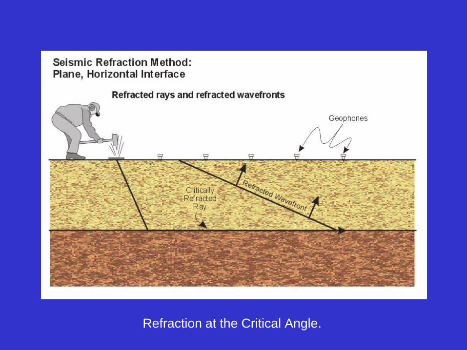
Refraction at the Critical Angle.
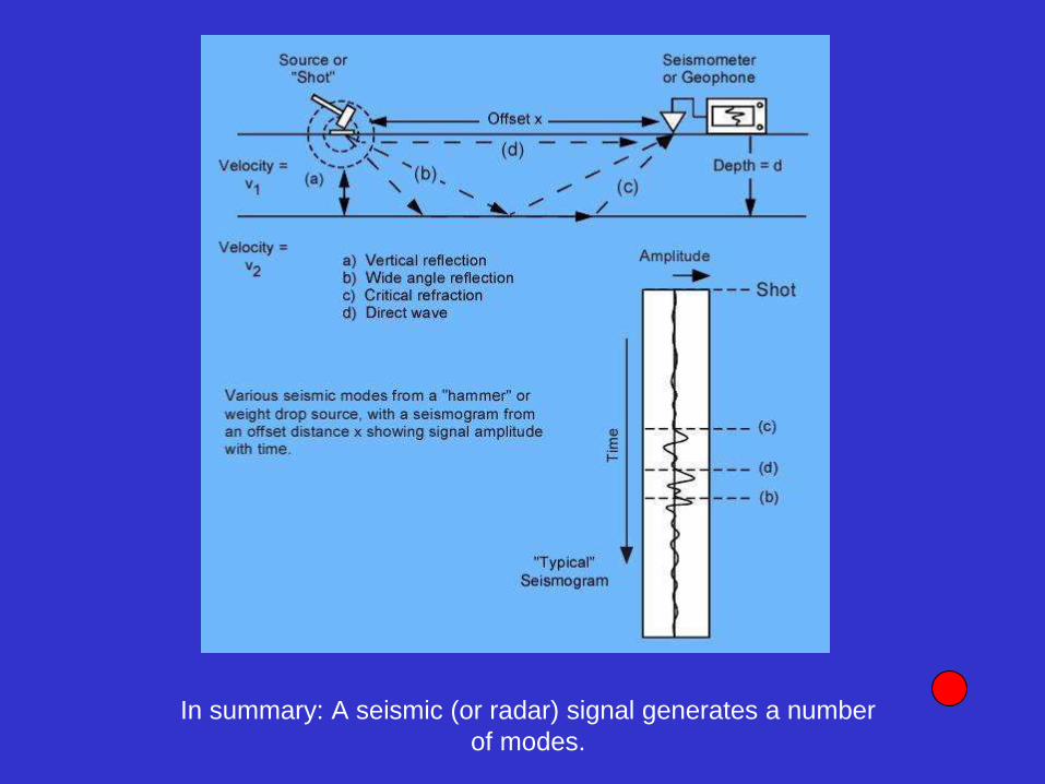
In summary: A seismic (or radar) signal generates a number
of modes.

How can we use the ‘refracted’ phase
to determine structure in the earth ?
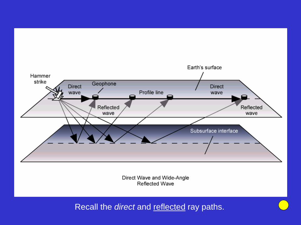
Recall the direct and reflected ray paths.

The direct and refracted ray paths.
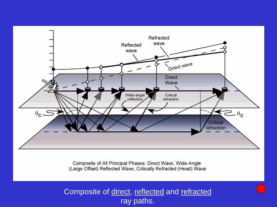
Composite of direct, reflected and refracted
ray paths.

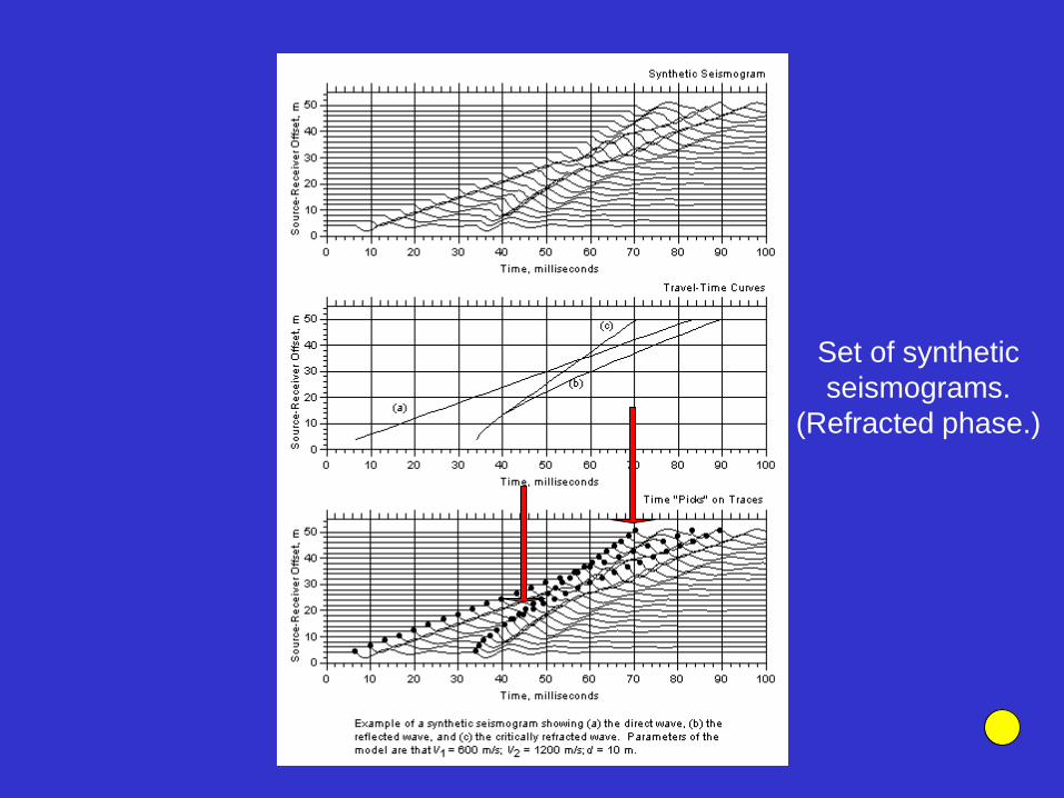
Set of synthetic
seismograms.

Details on “Picking” and Interpreting
Seismic Data
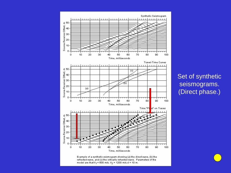
Set of synthetic
seismograms.
(Direct phase.)
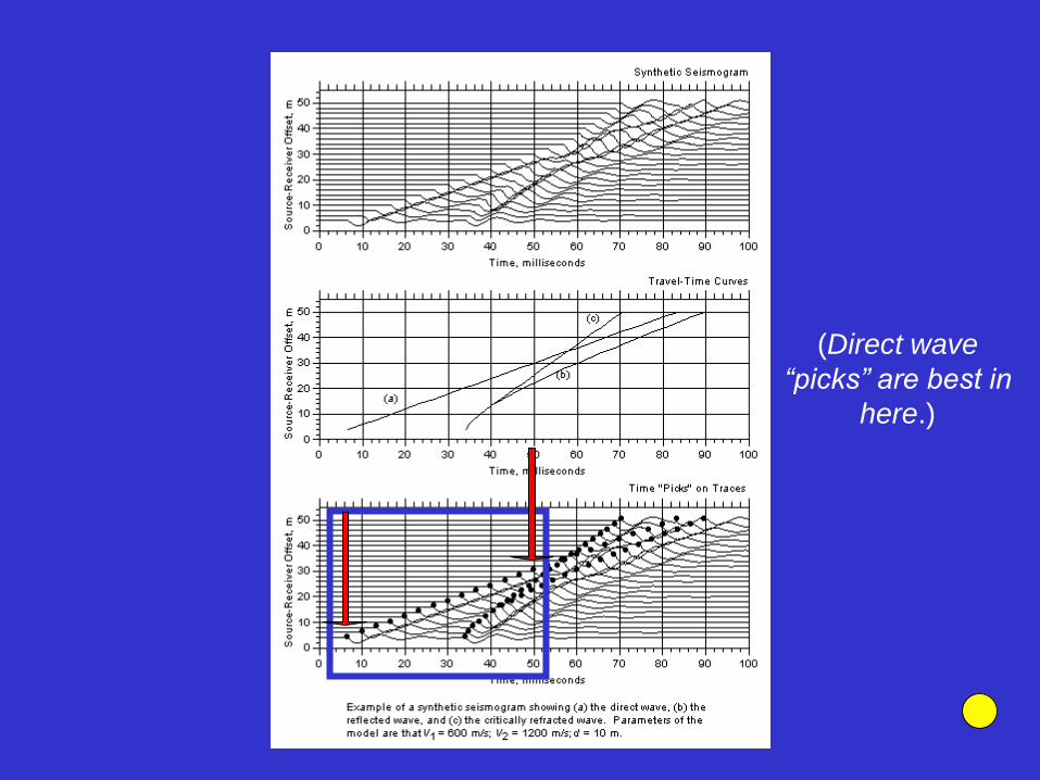
(Direct wave
“picks” are best in
here.)
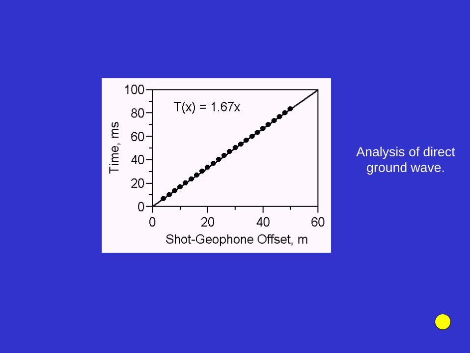
Analysis of direct
ground wave.
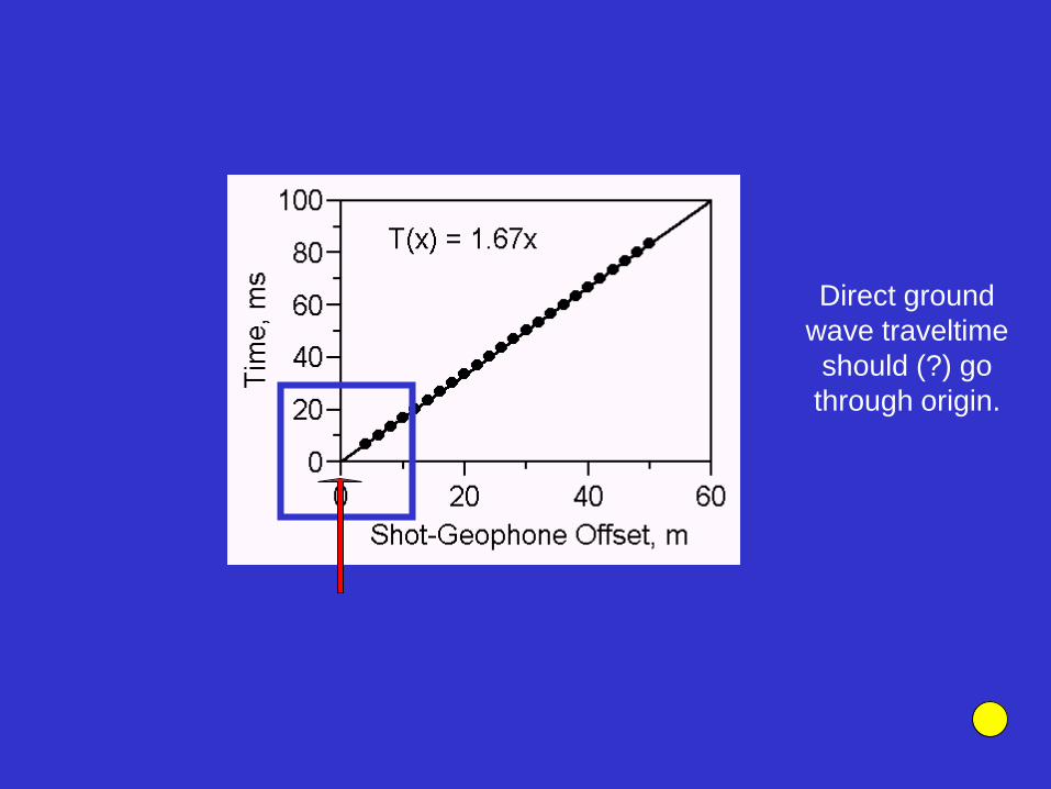
Direct ground
wave traveltime
should (?) go
through origin.
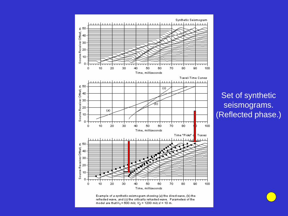
Set of synthetic
seismograms.
(Reflected phase.)
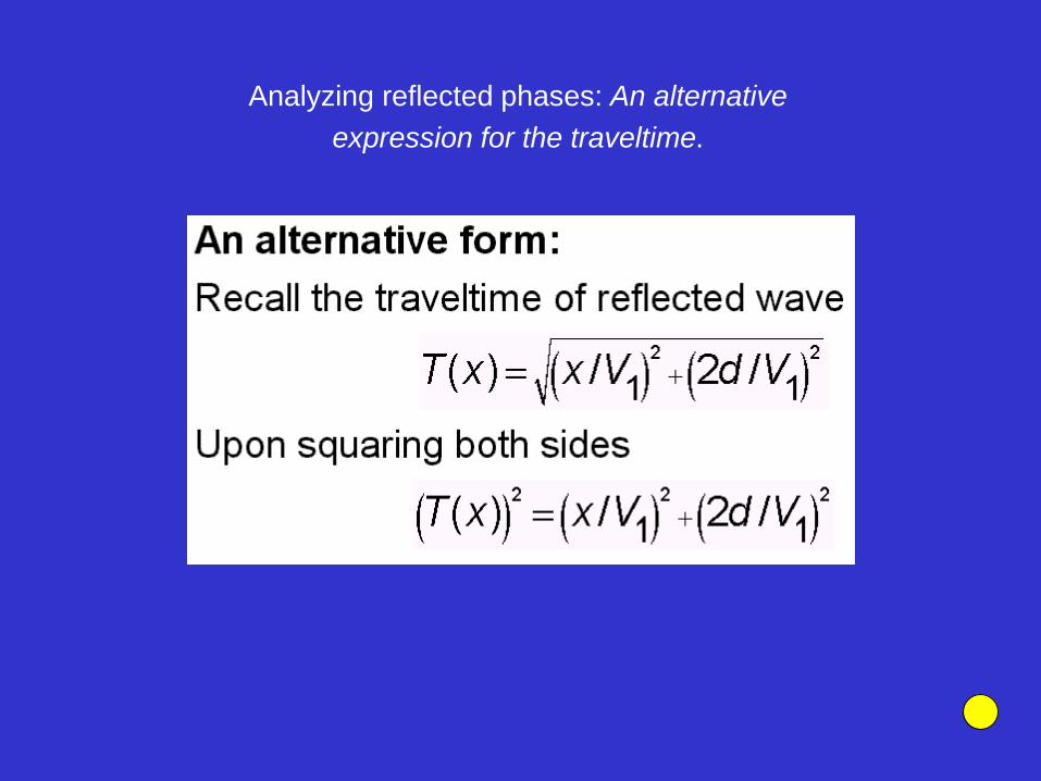
Analyzing reflected phases: An alternative
expression for the traveltime.
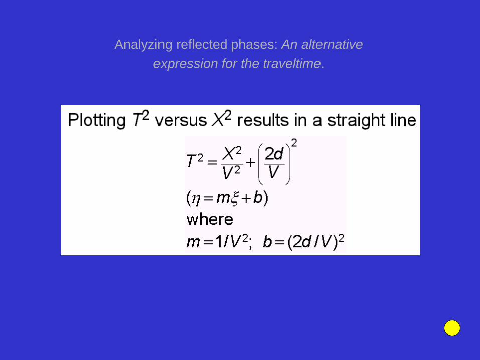
Analyzing reflected phases: An alternative
expression for the traveltime.
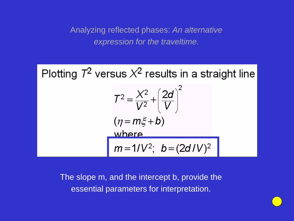
The slope m, and the intercept b, provide the
essential parameters for interpretation.
Analyzing reflected phases: An alternative
expression for the traveltime.
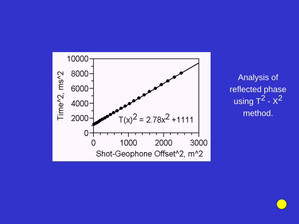
Analysis of
reflected phase
using T2 - X2
method.

Set of synthetic
seismograms.
(Refracted phase.)
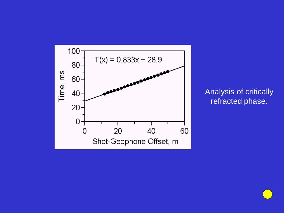
Analysis of critically
refracted phase.
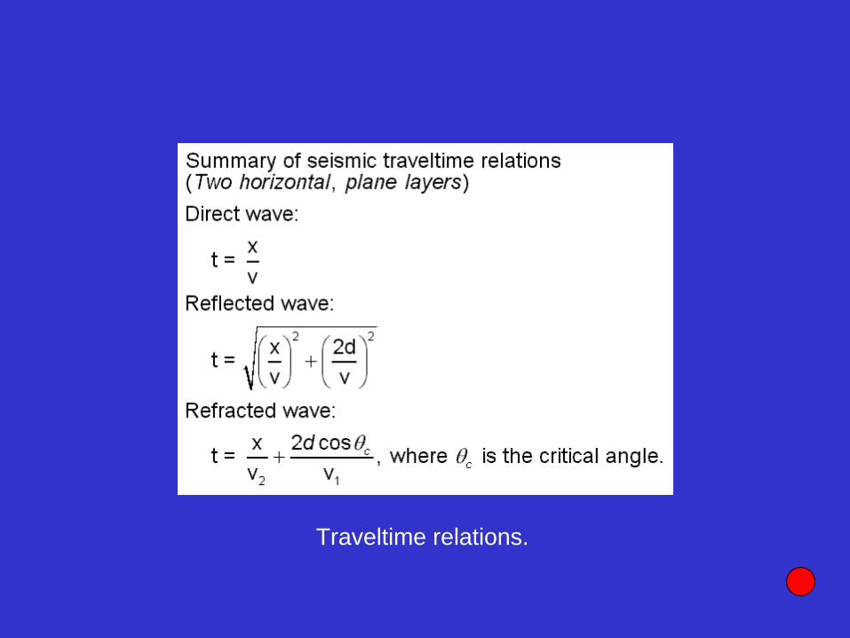
Traveltime relations.

Actual
seismogram
showing various
phases.

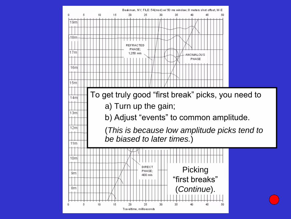
Picking
“first breaks”
(Continue).
Picking
“first breaks”
(Continue).
To get truly good “first break” picks, you need to
a) Turn up the gain;
b) Adjust “events” to common amplitude.
(This is because low amplitude picks tend to be biased to later times.)
Using the refraction method for more
complicated field situations.
Consider “dipping” interfaces.
Consider “dipping” interfaces.
We employ “reversed” refraction profiling.
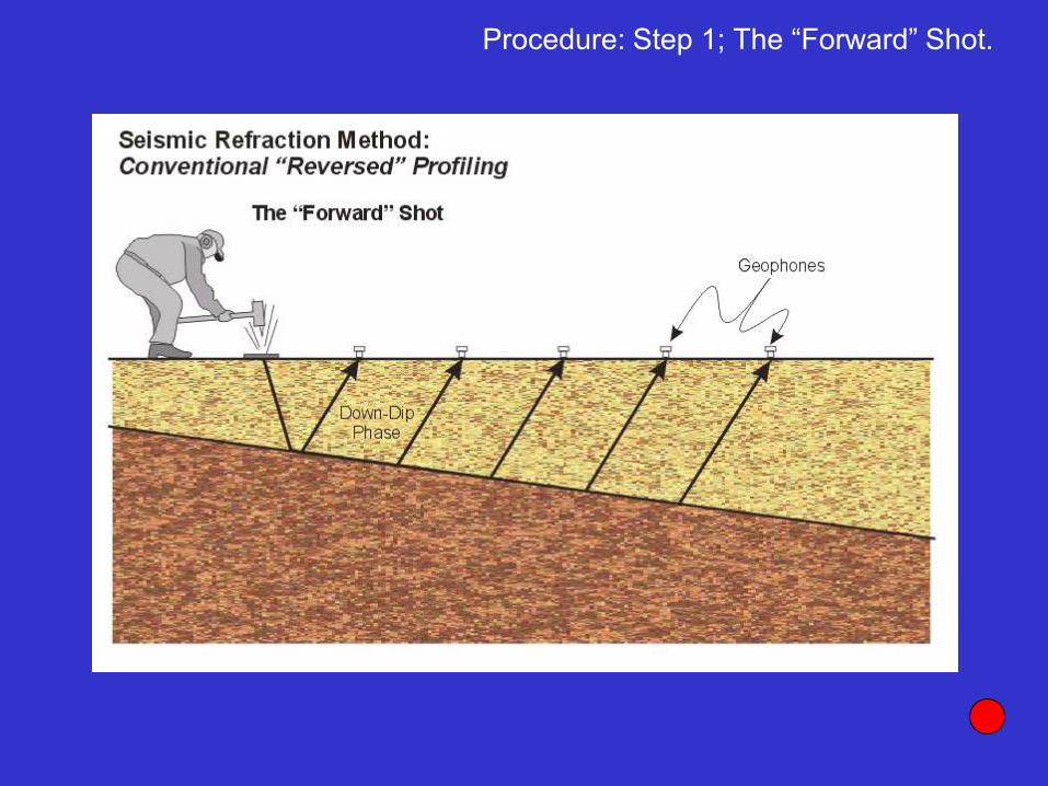
Procedure: Step 1; The “Forward” Shot.
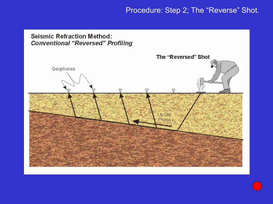
Procedure: Step 2; The “Reverse” Shot.
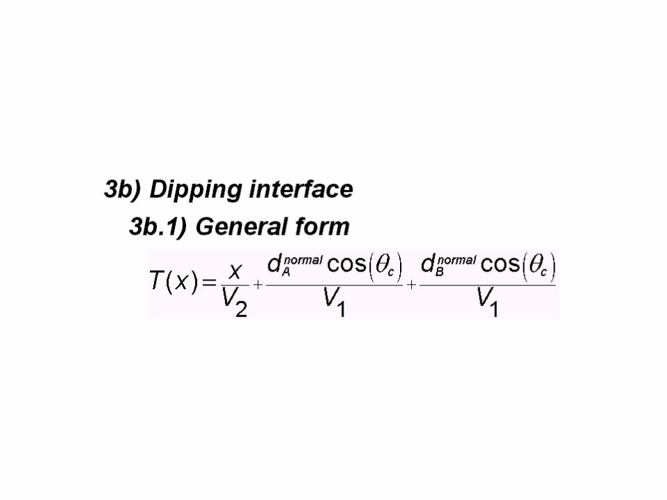
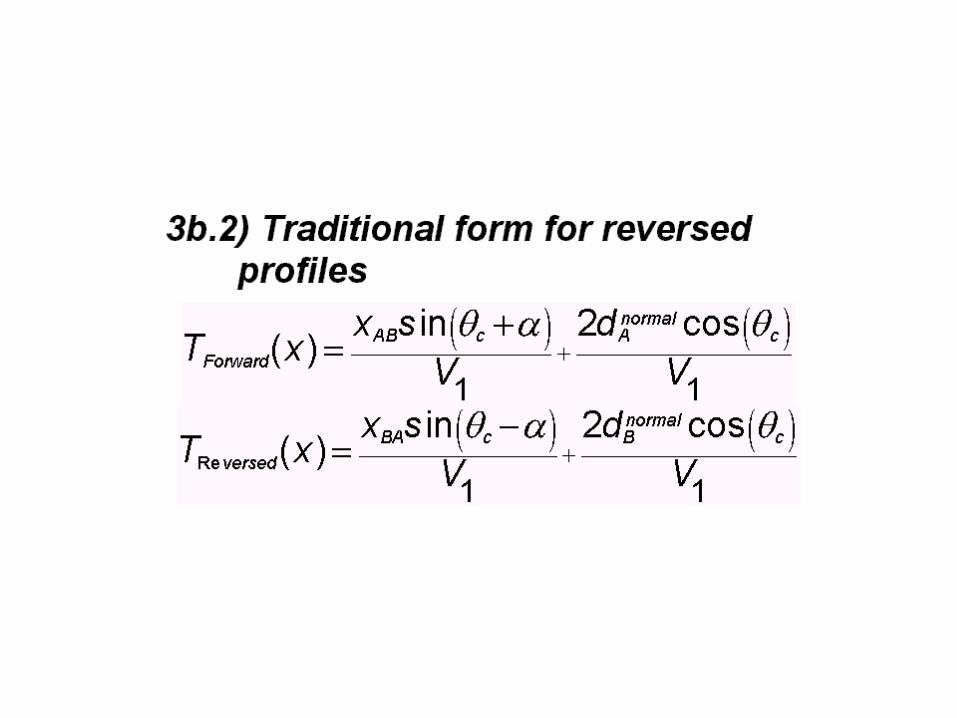
We use the theoretical traveltime of the respective
refracted phases.
September 1, 2002
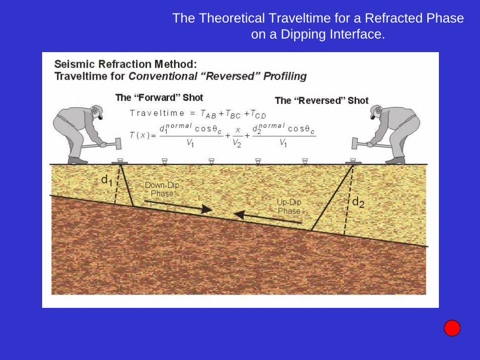
The Theoretical Traveltime for a Refracted Phase
on a Dipping Interface.
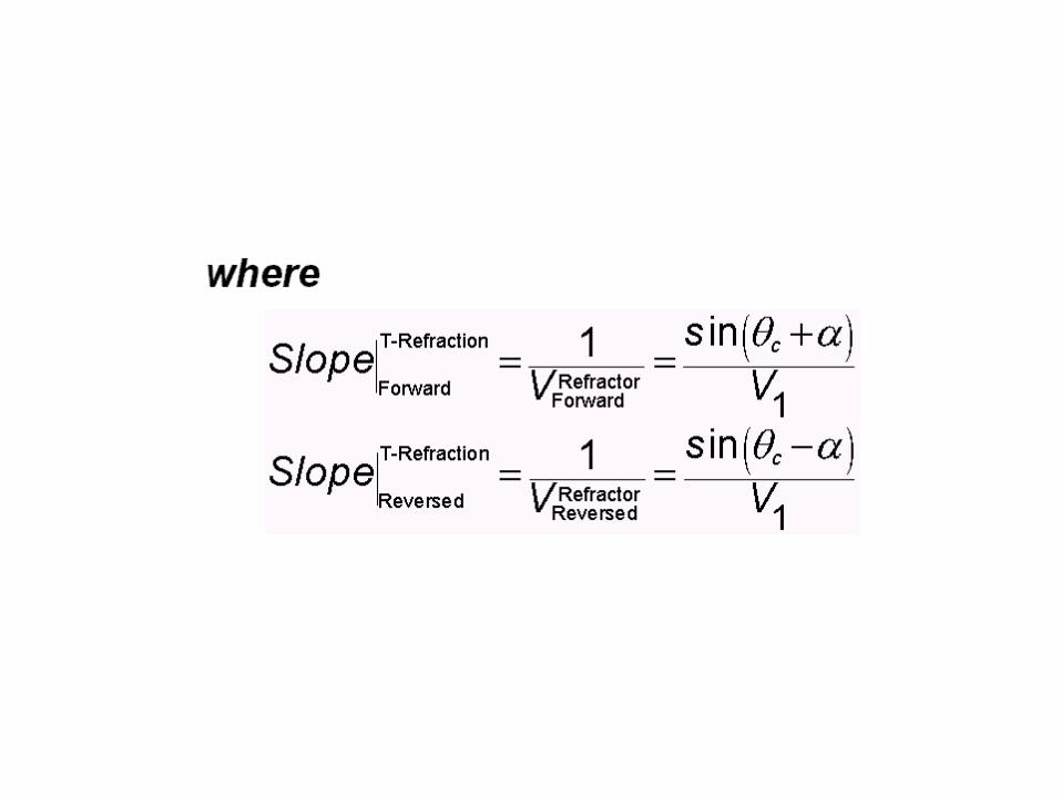
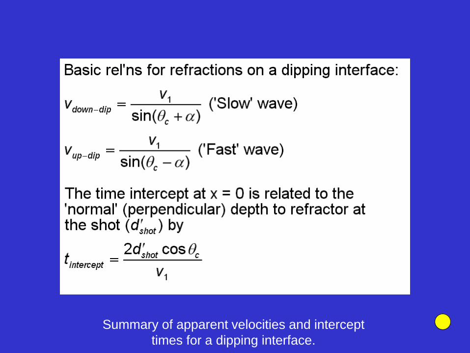
Summary of apparent velocities and intercept
times for a dipping interface.

How do we gather and interpret field data ?
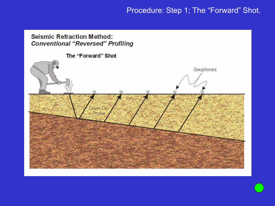
Procedure: Step 1; The “Forward” Shot.
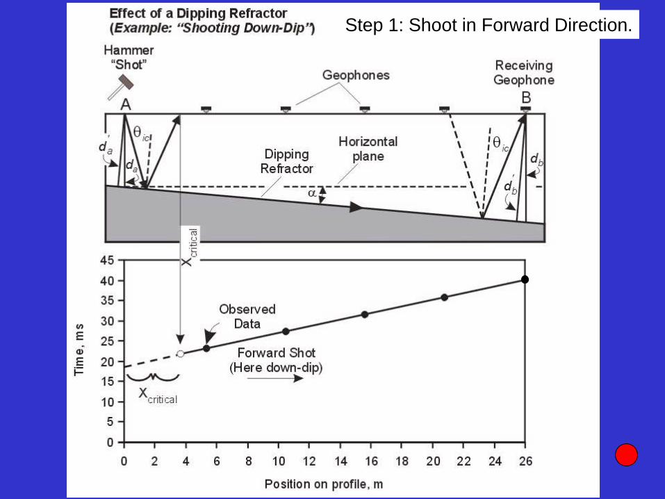
Step 1: Shoot in Forward Direction.
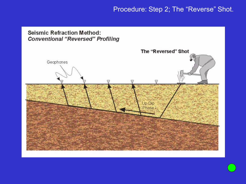
Procedure: Step 2; The “Reverse” Shot.
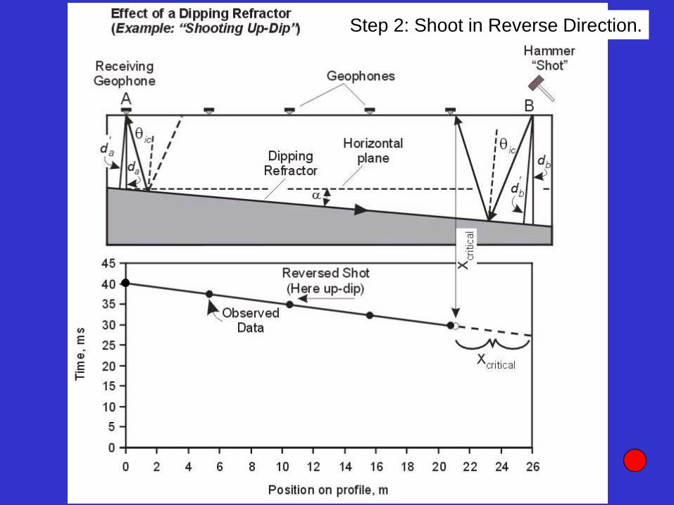
Step 2: Shoot in Reverse Direction.

Step 3: Inspect Data.

Step 4: Determine Forward Velocity.
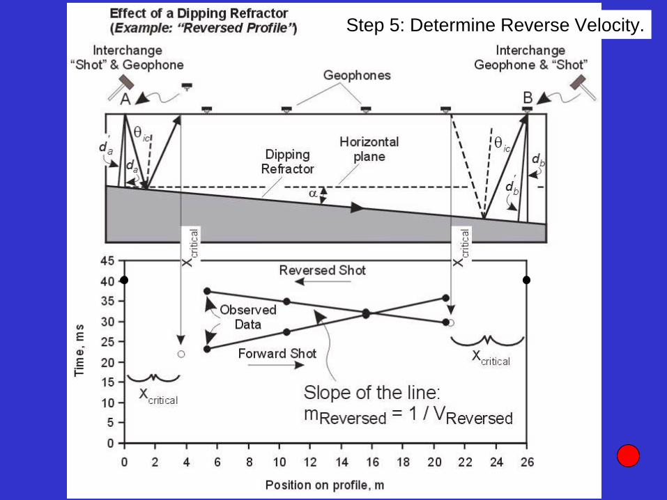
Step 5: Determine Reverse Velocity.
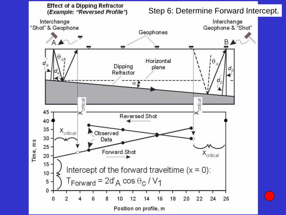
Step 6: Determine Forward Intercept.
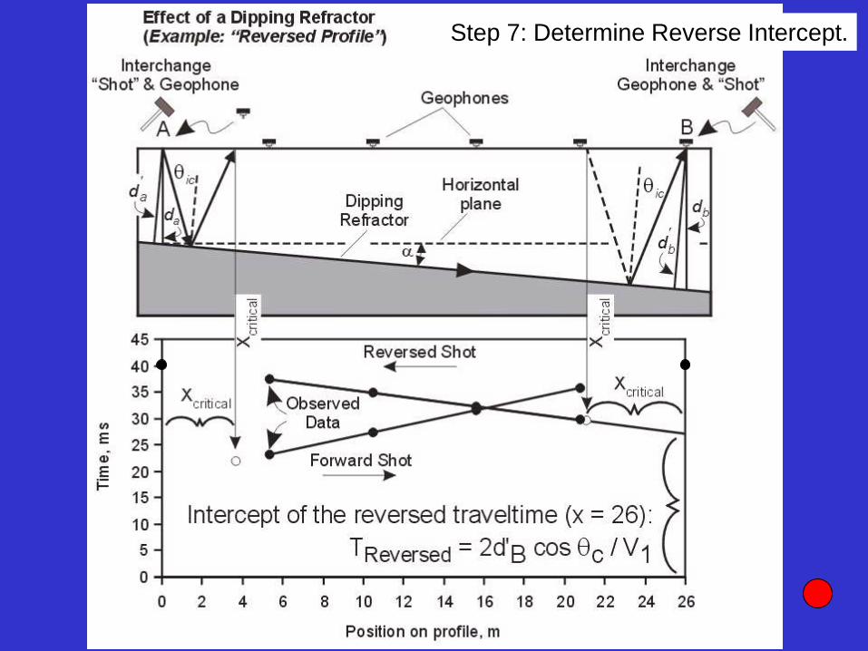
Step 7: Determine Reverse Intercept.
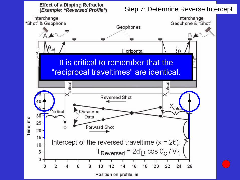
Step 7: Determine Reverse Intercept.
It is critical to remember that the
“reciprocal traveltimes” are identical.

Traveltime relations: Dipping refractor.

Some Examples.
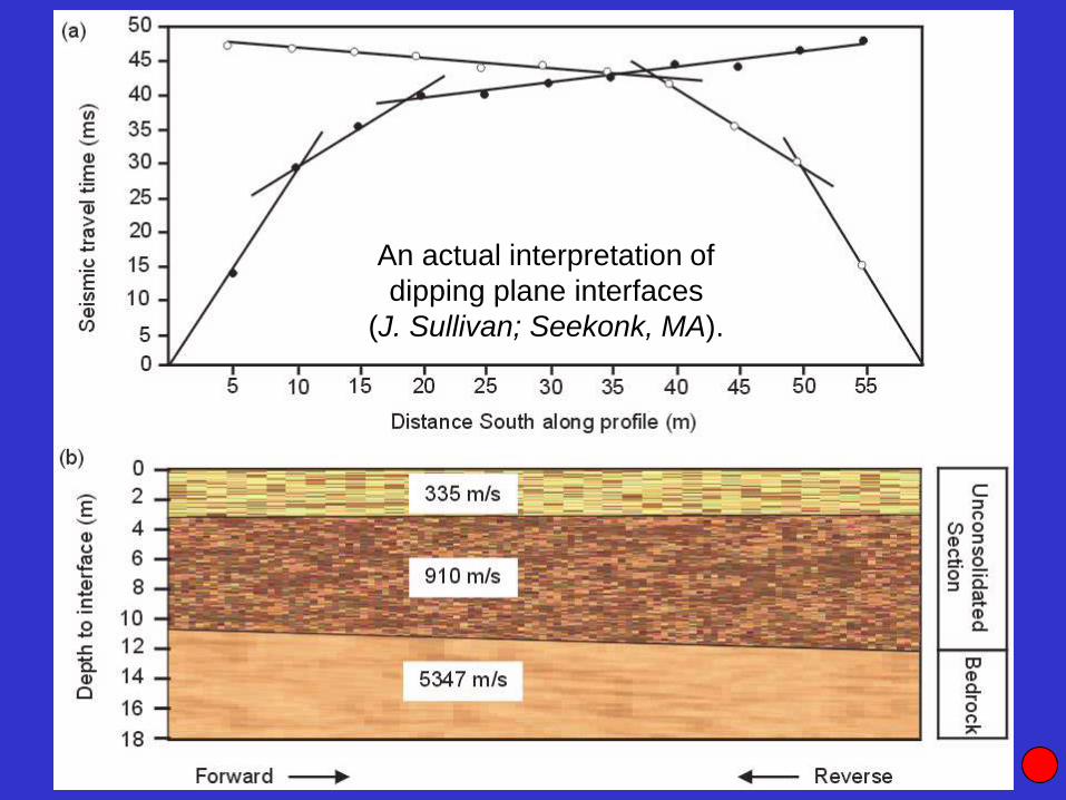
An actual interpretation of
dipping plane interfaces
(J. Sullivan; Seekonk, MA).
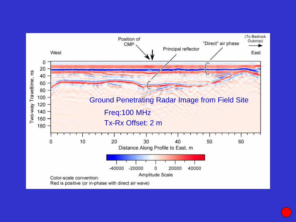
Characteristics of Field Area 1: Vertical GPR Time Section
Ground Penetrating Radar Image from Field Site
Freq:100 MHz
Tx-Rx Offset: 2 m
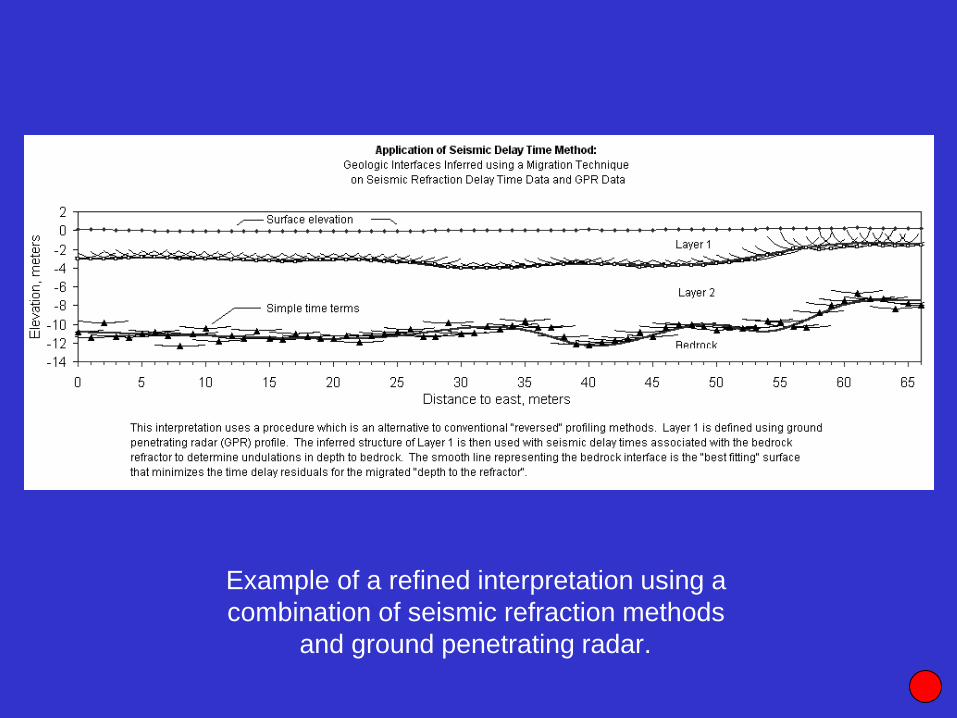
Example of a refined interpretation using a
combination of seismic refraction methods
and ground penetrating radar.
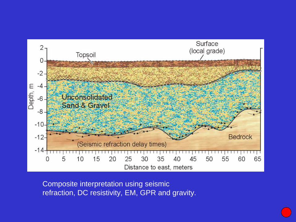
Subsurface structure above bedrock at field site.
Composite interpretation using seismic
refraction, DC resistivity, EM, GPR and gravity.
[Seismic interpretation from Jeff
Sullivan (personal communication.).]

Example of refraction study: Palmer River Basin.

In summary, a seismic interpretation depends on properly
identifying and time-picking appropriate phases.

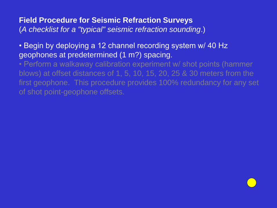
Field Procedure for Seismic Refraction Surveys
(A checklist for a "typical" seismic refraction sounding.)
• Begin by deploying a 12 channel recording system w/ 40 Hz
geophones at predetermined (1 m?) spacing.
• Begin by deploying a 12 channel recording system w/ 40 Hz
geophones at predetermined (1 m?) spacing.
• Perform a walkaway calibration experiment w/ shot points (hammer
blows) at offset distances of 1, 5, 10, 15, 20, 25 & 30 meters from the
first geophone. This procedure provides 100% redundancy for any set
of shot point-geophone offsets.
Field Procedure for Seismic Refraction Surveys
(A checklist for a "typical" seismic refraction sounding.)
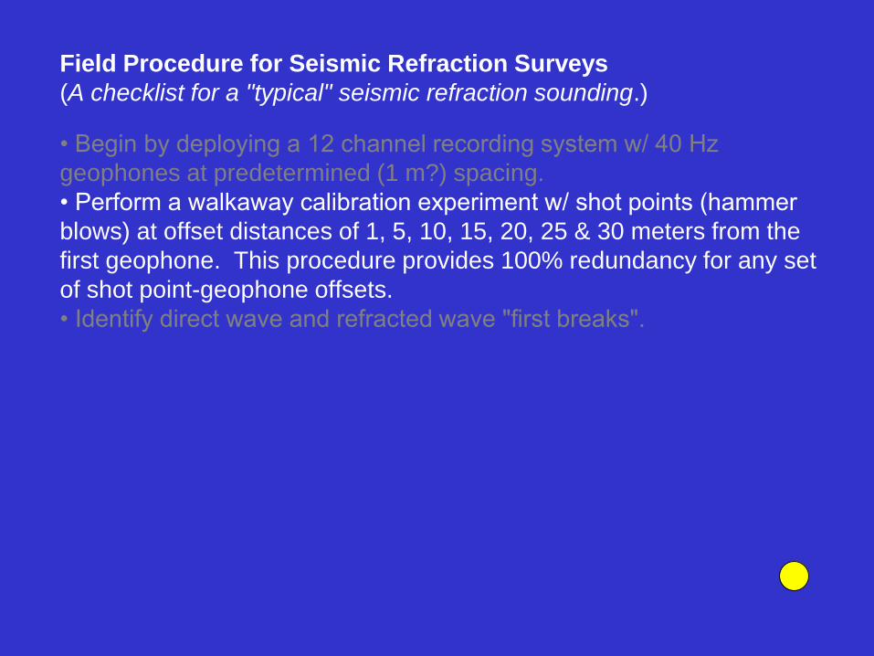
• Begin by deploying a 12 channel recording system w/ 40 Hz
geophones at predetermined (1 m?) spacing.
• Perform a walkaway calibration experiment w/ shot points (hammer
blows) at offset distances of 1, 5, 10, 15, 20, 25 & 30 meters from the
first geophone. This procedure provides 100% redundancy for any set
of shot point-geophone offsets.
• Identify direct wave and refracted wave "first breaks".
Field Procedure for Seismic Refraction Surveys
(A checklist for a "typical" seismic refraction sounding.)
• Begin by deploying a 12 channel recording system w/ 40 Hz
geophones at predetermined (1 m?) spacing.
• Perform a walkaway calibration experiment w/ shot points (hammer
blows) at offset distances of 1, 5, 10, 15, 20, 25 & 30 meters from the
first geophone. This procedure provides 100% redundancy for any set
of shot point-geophone offsets.
• Identify direct wave and refracted wave "first breaks".
• Reverse profile to identify dip on refractor.
• Based on these “calibration” runs, design an optimal field plan.
• Execute the optimized survey plan assuring adequate reciprocal shot
point-geophone data for both conventional reversed profiling as well as
a delay time analysis.
• Separate shot point time-terms from receiver time-terms.
• Shoot in orthogonal direction to determine dip and strike of refractor
in three dimensions.
Field Procedure for Seismic Refraction Surveys
(A checklist for a "typical" seismic refraction sounding.)
Each of these wave modes (or ‘phases’) provide useful, oftentimes
essential, information on the subsurface
In addition, strong analogies exist between
• Seismic (acoustic or mechanical) phenomena and
• Ground penetrating radar (electromagnetic) signals.

End of Presentation…
Thanks for Listen...