-

Structural Analysis

-

Semester 1 2016/2017

Department of Structures and Material Engineering

Faculty of Civil and Environmental Engineering

University Tun Hussein Onn Malaysia

Introduction

▪ The primary purpose of structural analysis is to establish thedistribution of internal forces and moments over the wholepart of a structure and to identify the critical design conditionsat all sections.

▪ The type of analysis should appropriate to the problem beingconsidered.

▪ The following approach can be used: linear elastic analysis,linear elastic analysis with limited redistribution, andplastic analysis.

▪ Linear elastic analysis can be carried out by assuming thatthe cross section is uncracked (i.e. concrete sectionproperties), involves linear stress-strain relationships andmean value of elastic modulus.

▪ Plastic analysis is desired in the design consideration,however, this approach requires advanced solutions.

Introduction

Distribution of actions on slab

Action on slab and wall transfer

to beam

Axial load on column

Distribute to foundation

Structural Layout

▪ Before any analysis and design can be conducted, structurallayout (key-plan) must be produced.

▪ Structural layout planning is always started from the lowestfloor. Step to produce structural layout:

− Study and understand the architectural drawings (floorplans, elevations, cross sections, isometric view, specificdetails and so on).

− Identify location and orientation of columns.

− Identify location and position of beams.

− Sketch the structural plans.

▪ For a simple layout, structural layout can be sketched on thearchitectural drawing by using colour pencil.

▪ For a complex layout, structural layout can be sketched on thebutter paper by tracing from the architectural drawing.

Structural Layout

▪ Location, orientation and dimension of columns:

• Some are stated in the architectural drawings.

• At the corner and intersection.

• The distance between column and column is not too farand too close. Typically about 3m to 6m.

• Flush with brickwall

▪ Location, position and dimension of beams

• Location of brickwall, to brace the columns, to flush andbrace the brickwall, to form spanning slab.

• Dimension of beam is governed by thickness of brickwall,types of building, type of floor (ground or upper floor, upperfloor with or without ceiling, head room), span andarchitectural drawing.

Structural LayoutA

rch

ite

ctu

ral p

lan

Structural LayoutE

ngin

ee

rin

g L

ayout

Analysis of Actions

▪ Actions that applied on a beam may consist of beams self-

weight, permanent and variable actions from slabs, actions

from secondary beams and other structural or non-structural

members supported by the beam.

▪ The distribution of slab actions on beams depends on the slab

dimension, supporting system and boundary condition.

▪ It is important to determine the type of slab using following

criteria:

2y

x

L

L

2y

x

L

L

One-way slab

Two-way slab

Analysis of Actions

▪ Type of actions that must be considered:

Slab ✓Permanent action: (i) Selfweight of slab,

(ii) Finishes and services, and (iii) Ceiling

✓Variable action (depend on function of floor)

Beam ✓Permanent action: (i) Distribution from slab,

(ii) Selfweight of beam, and (iii) Brickwall

✓Variable action from slab

Column ✓Permanent action: (i) Distribution from beam,

and (ii) selfweight of column

✓Variable action from beam

Foundation ✓Permanent action: (i) Distribution from

columns, and (ii) selfweight of footing

✓Variable action from column

Analysis of Actions

▪ One-way spanning slab that supported by beams:

lx

ly

A B

C D

ly

w = 0.5.n.lx kN/m

Beam AC and BD

lx

w = 0 kN/m

Beam AB and CD

Analysis of Actions

▪ Two-way slab panel freely supported along four edge:

lx

ly

A B

C D

ly

mkNl

lnlw

y

xx /36

2

−=

Beam AC and BD

lx

mkNnl

w x /3

=

Beam AB and CD

How about if lx = ly?

Analysis of Actions

▪ There are alternatives methods which consider various

support conditions and slab continuity. The methods are

(i). Slab shear coefficient from Table 3.15 BS 8110, (ii). Yield

line analysis and (iii). Table 63 Reinforced Concrete

Designer’s Handbook by Reynold.

This table only can be used for two-way slabs. The type of spanning slab (from 9 cases) must be identified first.

Analysis of Actions

▪ Two-way spanning slab:

lx

ly

A B

C D

ly

w = βvx.n.lx kN/m

Beam AC

lx

Beam CD

w = βvy.n.lx kN/m

Analysis of Actions

9 cases of

two-way

restrained

slab

Analysis of Actions

Case 1

Case 2

Case 3

Case 4

Case 5

Case 6

Case 7

Case 8

Case 9

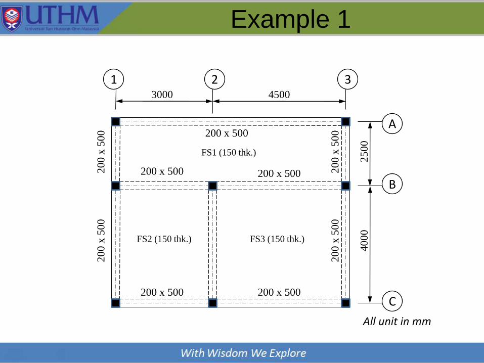
Example 1

▪ Determine the characteristic permanent and variable actionon beam B/1-3.Given the following data: Unit weight ofconcrete = 25kN/m3; Finishes, ceiling and services =2.0kN/m2;Variable action (all slabs) = 3.0kN/m2.

Action on slab:

Selfweight = 0.15 x 25 = 3.75 kN/m2

Finishes, ceiling and services = 2.0 kN/m2

Chac. Permanent action, Gk = 5.75 kN/m2

Chac. Variable action, Qk = 3.0 kN/m2

Distribution of actions

FS1 : ly/lx = 7.5 / 2.5 = 3 > 2.0, One-way slab

FS2 : ly/lx = 4.0 / 3.0 = 1.33 < 2.0, Two-way slab

FS3 : ly/lx = 4.5 / 4.0 = 1.13 < 2.0, Two-way slab

Example 1

3000 4500

25

00

40

00

1 2 3

A

B

C

200 x 500

200 x 500 200 x 500

200 x 500 200 x 500

20

0 x

50

02

00

x 5

00

20

0 x

50

02

00

x 5

00

FS1 (150 thk.)

FS2 (150 thk.) FS3 (150 thk.)

All unit in mm

Example 1

3000 4500

25

00

40

00

1 2 3

A

B

C

All unit in mm

w1 = 0.5.n.lx

w2 = βvy.n.lxw3 = βvx.n.lx

Example 1

Action from slab:

w1 Gk = 0.5 x 5.75 x 2.5 = 7.19 kN/m

w1 Qk = 0.5 x 3.00 x 2.5 = 3.75 kN/m

From Table 3.15: BS 8110: Part 1: 1997

w2 Gk = 0.4 x 5.75 x 3.0 = 6.90 kN/m

w2 Qk = 0.4 x 3.00 x 3.0 = 3.60 kN/m

w3 Gk = 0.44 x 5.75 x 4.0 = 10.12 kN/m

w3 Qk = 0.44 x 3.00 x 4.0 = 5.28 kN/m

Example 1

Actions on beam:

Beam selfweight = 0.20x(0.5–0.15)x25 = 1.75 kN/m

Span 1-2

Permanent action,Gk = 7.19+6.90+1.75 = 15.84 kN/m

Variable action, Qk = 3.75+3.60 = 7.35 kN/m

Span 2-3

Permanent action, Gk = 7.19+10.12+1.75 = 19.06 kN/m

Variable action, Qk = 3.75+5.28 = 9.03 kN/m

3000 4500

Gk = 15.84 kN/mQk = 7.35 kN/m

Gk = 19.06 kN/mQk = 9.03 kN/m

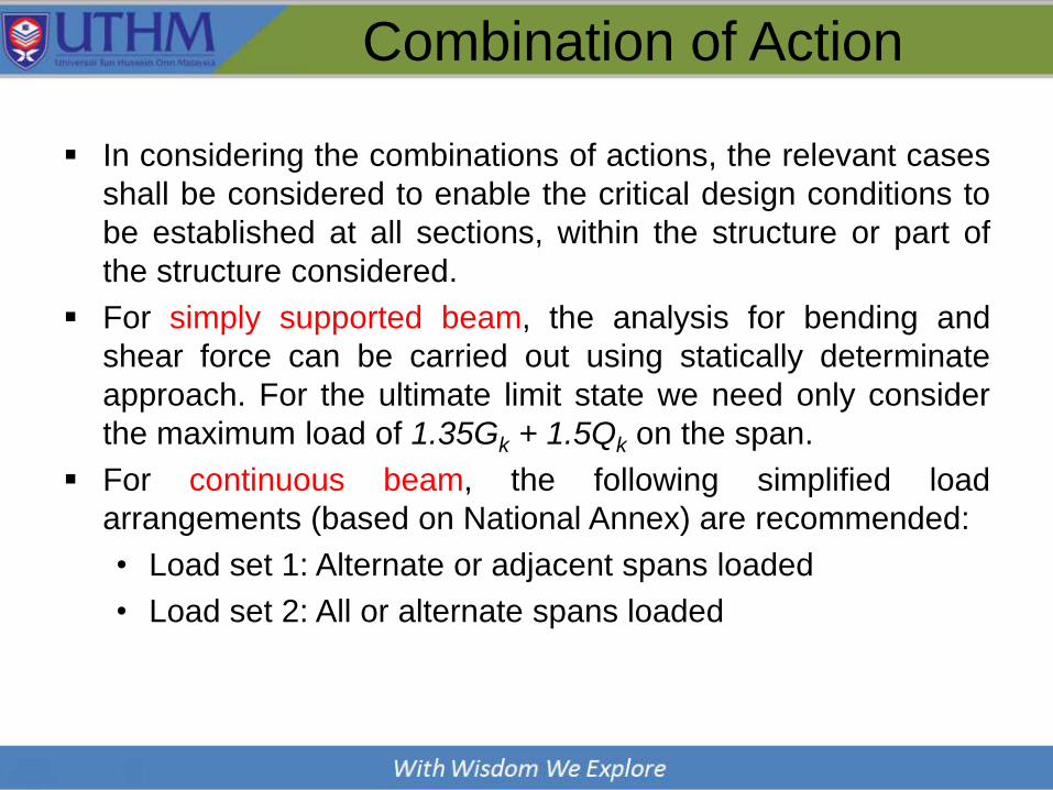
Combination of Action

▪ “Combination of action” is specifically used for the definition of

the magnitude of actions to be used when a limit state is

under the influence of different actions.

▪ For continuous beam, “Load cases” is concerned with the

arrangement of the variable actions to give the most

unfavourable conditions or most critical responses.

▪ If there is only one variable actions (e.g. imposed load) in a

combination, the magnitude of the actions can be obtained by

multiplying with the appropriate factors.

▪ If there is more than one variable actions in combination, it is

necessary to identify the leading action(Qk,1) and other

accompanying actions (Qk,i). The accompanying actions is

always taken as the combination value.

Combination of Action

▪ In considering the combinations of actions, the relevant cases

shall be considered to enable the critical design conditions to

be established at all sections, within the structure or part of

the structure considered.

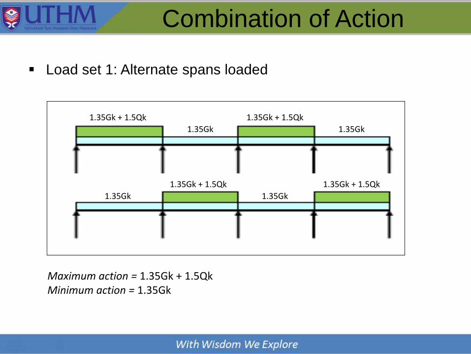
▪ For simply supported beam, the analysis for bending and

shear force can be carried out using statically determinate

approach. For the ultimate limit state we need only consider

the maximum load of 1.35Gk + 1.5Qk on the span.

▪ For continuous beam, the following simplified load

arrangements (based on National Annex) are recommended:

• Load set 1: Alternate or adjacent spans loaded

• Load set 2: All or alternate spans loaded

Combination of Action

▪ Load set 1: Alternate or adjacent spans loaded

(Section 5.1.3 : MS EN 1992-1-1)

– Alternate span carrying the design permanent and variableload (1.35Gk + 1.5Qk), other spans carrying only thedesign permanent loads (1.35Gk)

– Any two adjacent spans carrying the design permanentand variable loads (1.35Gk + 1.5Qk), all other spanscarrying only the design permanent load (1.35Gk)

▪ Load set 2: All or alternate spans loaded

(UK National Annex)

– All span carrying the design permanent and variable loads(1.35Gk+ 1.5Qk)

– Alternate span carrying the design permanent and variableload (1.35Gk+ 1.5Qk), other spans carrying only thedesign permanent loads (1.35Gk)

Combination of Action

▪ Load set 1: Alternate spans loaded

1.35Gk + 1.5Qk

1.35Gk

1.35Gk + 1.5Qk

1.35Gk

1.35Gk + 1.5Qk

1.35Gk

1.35Gk + 1.5Qk

1.35Gk

1.35Gk + 1.5Qk

1.35Gk

1.35Gk + 1.5Qk

1.35Gk

1.35Gk + 1.5Qk

1.35Gk

1.35Gk + 1.5Qk

1.35Gk

Maximum action = 1.35Gk + 1.5QkMinimum action = 1.35Gk

Combination of Action

▪ Load set 1: Adjacent Span Loaded

1.35Gk + 1.5Qk

1.35Gk

1.35Gk + 1.5Qk

1.35Gk

1.35Gk + 1.5Qk

1.35Gk

1.35Gk + 1.5Qk

1.35Gk

1.35Gk + 1.5Qk1.35Gk 1.35Gk

1.35Gk + 1.5Qk

1.35Gk + 1.5Qk 1.35Gk + 1.5Qk

1.35Gk 1.35Gk

1.35Gk + 1.5Qk 1.35Gk + 1.5Qk1.35Gk 1.35Gk

Combination of Action

▪ Load set 2: All span loaded

▪ Load set 2: Alternate span loaded

1.35Gk + 1.5Qk 1.35Gk + 1.5Qk 1.35Gk + 1.5Qk 1.35Gk + 1.5Qk

1.35Gk + 1.5Qk 1.35Gk + 1.5Qk

1.35Gk 1.35Gk

1.35Gk

1.35Gk + 1.5Qk 1.35Gk + 1.5Qk

1.35Gk

Moment and Shear Force

▪ The shear force and bending moment diagrams can be drawn

for each of the load cases required in the patterns of loading.

▪ A composite diagram comprising a profile indicating the

maximum values including all possible load cases can be

drawn; this is known as an envelope.

▪ Three analysis methods may be used in order to obtain shear

force and bending moment for design purposes. There are;

Elastic analysis using moment distribution method

(Modified Stiffness Method)

Simplified method using shear and moment coefficient

from Table 3.6: BS 8110: Part 1.

Using commercial analysis software such as Staad.Pro,

Esteem, Ansys, Lusas, etc.

Moment and Shear Force

▪ Envelope moment and shear force:

Load Case 1 Load Case 2

SFD

BMD

SFD

BMD

Moment and Shear Force

▪ Envelope moment and shear force:

Load Case 3

SFD

BMD

SHEAR FORCE DIAGRAM ENVELOPE

BENDING MOMENT DIAGRAM ENVELOPE

Moment Distribution Method

▪ Moment distribution method is only involving distribution

moments to joint repetitively.

▪ The accuracy of moment distribution method is dependent to

the number repeat which does and usually more than 5 repeat

real enough. Right value will be acquired when no more

moments that need distributed.

▪ In general the value is dependent to several factor as :

• Fixed end moment - the moment at the fixed joints of a

loaded member.

• Carry over factor - the carry-over factor to a fixed end is

always 0.5, otherwise it is zero.

• Member stiffness factor (distribution factor) – need to be

determined based on moment of inertia and stiffness.

Simplified Method

▪ The analysis using Moment Distribution Method is time

consuming.

▪ Therefore, as a simplification, Cl. 3.4.3 BS 8110 (Table 3.5)

can be used. This simplified method enables a conservative

estimation of shear force and bending moment for continuous

beam.

▪ However, there are conditions which must be satisfied:

• The beams should be approximately equal span.

• Variation in span length should not exceed 15% of the

longest span.

• The characteristic variable action, Qk may not exceed the

characteristic permanent action, Gk.

• Load should be substantially uniformly distributed over

three or more spans.

Simplified Method

▪ The

(1.35Gk + 1.5Qk)

-0.11FL

0.09FL

-0.08FL -0.08FL

0.07FL

0.45F

0.60F

0.55F

0.55F

End Span Interior Span

Bending Moments

Shearing Forces

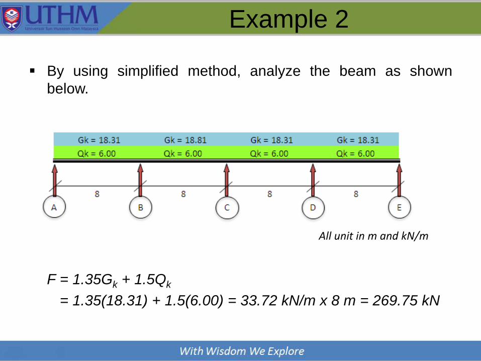
Example 2

▪ By using simplified method, analyze the beam as shown

below.

F = 1.35Gk + 1.5Qk

F = 1.35(18.31) + 1.5(6.00) = 33.72 kN/m x 8 m = 269.75 kN

All unit in m and kN/m

Example 2

Shear force and bending moment diagrams

0.45F =121.39 kN

0.60F =161.85 kN

0.55F =148.36 kN 0.55F =148.36 kN

0.55F =148.36 kN 0.55F =148.36 kN

0.60F =161.85 kN

0.45F =121.39 kN

0.09FL =194.22 kNm

0.11FL =237.38 kNm 0.08FL =172.64kNm 0.11FL =237.38 kNm

0.07FL =151.06 kNm 0.07FL =151.06 kNm 0.09FL =194.22 kNm

Moment Redistribution

▪ Plastic behavior of RC at the ULS affects the distribution of

moment in structure.

▪ To allow for this, the moment derived from an elastic analysis

may be redistributed based on the assumption that plastic

hinges have formed at the sections with the largest moment.

▪ From design point of view, some of elastic moment at support

can be reduced, but this will increasing others to maintain the

static equilibrium of the structure.

▪ The purpose or moment redistribution is to reduced the

bending moment at congested zone especially at beam-

column connection of continuous beam support.

▪ Therefore, the amount of reinforcement at congested zone

also can be reduced then it will result the design and detailing

process become much easier.

Moment Redistribution

▪ Section 5.5 EC2 permit the moment redistribution with the

following requirement;

• The resulting distribution remains in equilibrium with the

load

• The continuous beam are predominantly subject to flexural

• The ratio of adjacent span should be in the range of 0.5 to

2

▪ There are other restrictions on the amount of moment

redistribution in order to ensure ductility of the beam such as

grade of reinforcing steel and area of tensile reinforcement

and hence the depth of neutral axis.

• Class A reinforcement; redistribution should ≤ 20%

• Class B and C reinforcement; redistribution should ≤ 30%

Example 3

▪ For the moments obtained from Moment Distribution Method,

redistribute 20% of moment at supports.

Example 3

Redistribute the moment at support

Original moment at support B & D = 231.21 kNm

Reduced moment (20%) = 0.8x231.21 = 184.97 kNm

Original moment at support C = 154.14 kNm

Reduced moment (20%) = 0.8x154.14 = 123.31 kNm

Recalculate the shear force using equilibrium principles.

Example 3

33.72 kN/m

8 m

VA VB1

ΣMB = 0

VA(8) – 33.72(8)2/2 + 184.97 = 0

VA = 894.07 / 8 = 111.76 kN

ΣFy = 0

111.76 + VB1 – 33.72(8) = 0

VB1 = 158.0 kN

ΣMC = 0

VB2(8) – 33.72(8)2/2 + 123.21 - 184.97 = 0

VB2 = 1140.8 / 8 = 142.60 kN

ΣFy = 0

142.60 + VC1 – 33.72(8) = 0

VC1 = 127.16 kN

33.72 kN/m

8 m

123.21 kNm

VC1VB2

184.97 kNm

Span A - B

Span B - C

184.97 kNm

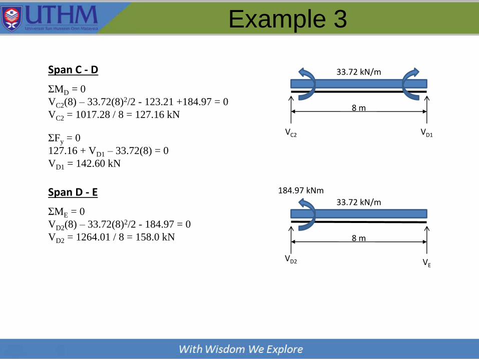
Example 3

33.72 kN/m

8 m

VC2 VD1

ΣMD = 0

VC2(8) – 33.72(8)2/2 - 123.21 +184.97 = 0

VC2 = 1017.28 / 8 = 127.16 kN

ΣFy = 0

127.16 + VD1 – 33.72(8) = 0

VD1 = 142.60 kN

ΣME = 0

VD2(8) – 33.72(8)2/2 - 184.97 = 0

VD2 = 1264.01 / 8 = 158.0 kN

33.72 kN/m

8 m

VEVD2

184.97 kNm

Span C - D

Span D - E