Introduction to Randomized Matrix Algorithms

Ilse Ipsen

Students: John Holodnak, Thomas Wentworth

Research supported by NSF CISE CCF, NSF DMS, DARPA XData

Randomized algorithms

Solve a deterministic problem by statistical sampling

Monte Carlo methodsVon Neumann & Ulam, Los Alamos, 1946

Simulated annealing: global optimization

This talk

Given: Real matrix A with more columns than rowsWant: Monte Carlo algorithm for matrix product AAT

Why is this important?

Monte Carlo algorithm produces approximation X = BBT

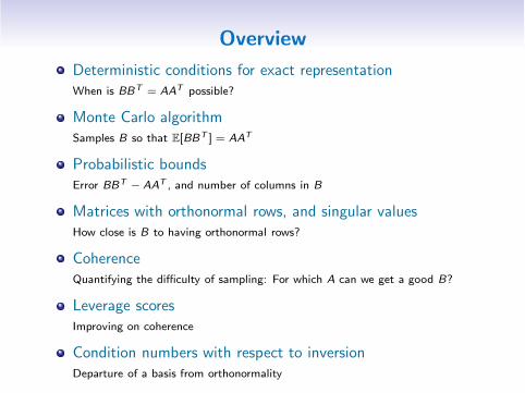
Overview

Deterministic conditions for exact representationWhen is BBT = AAT possible?

Monte Carlo algorithmSamples B so that E[BBT ] = AAT

Probabilistic boundsError BBT − AAT , and number of columns in B

Matrices with orthonormal rows, and singular valuesHow close is B to having orthonormal rows?

CoherenceQuantifying the difficulty of sampling: For which A can we get a good B?

Leverage scoresImproving on coherence

Condition numbers with respect to inversionDeparture of a basis from orthonormality

Deterministic conditionsfor exact representation

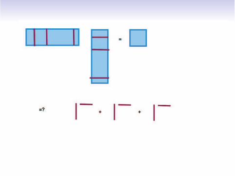
Gram product: AAT

Real matrix A =(

A1 . . . An

)

with n columns

Exact computation

AAT = A1AT1 + · · · + AnA

Tn

Monte Carlo algorithm [Drineas, Kannan & Mahoney]

Sample c columns

X = w1 At1ATt1 + · · ·+ wc AtcA

Ttc

wj ≥ 0 chosen so that X is unbiased estimator

E[X ] = AAT

Gram product: AAT

Real matrix A =(

A1 . . . An

)

with n columns

Exact computation

AAT = A1AT1 + · · · + AnA

Tn

Monte Carlo algorithm [Drineas, Kannan & Mahoney]

Sample c columns

X = w1 At1ATt1 + · · ·+ wc AtcA

Ttc

Weights wj ≥ 0 chosen so that X is unbiased estimator

E[X ] = AAT

Existing work

Randomized matrix multiplication

Cohen & Lewis 1997, 1999Rudelson 1999, Drineas & Kannan 2001Frieze, Kannan & Vempala 2004Drineas, Kannan & Mahoney 2006, Sarlos 2006Rudelson & Vershynin 2007Belabbas & Wolfe 2008Magdon-Ismail 2010, Drineas & Zouzias 2010, Magen & Zouzias 2010Pagh 2011Hsu, Kakade & Zhang 2012, Li, Miller & Peng 2012Liberty 2013

Connections toMatrix concentration (Minsker, Tropp, ...)Low-rank approximations, subset selection (Boutsidis, ...)Nystrom approximations (Gittens, ...)Graph sparsification (Spielman, Srivastava, ...)Compressed sensing (Donoho, Candes, ...)Matrix completion (Recht, ...)

Why is this a good idea?

Want:AAT = A1A

T1 + · · · + AnA

Tn

Monte Carlo algorithm:

X = w1 At1ATt1 + · · · + wc AtcA

Ttc

Why should c columns produce a good approximation?

How to determine the columns and weights?

Use the SVD

Singular Value Decomposition (SVD)

Real m × n matrix A with rank(A) = r

A = U Σ V T

Left singular vector matrixU is m × r with orthonormal columns: UTU = Ir

Right singular vector matrixV is n × r with orthonormal columns: V TV = Ir

Singular values

Σ =

σ1. . .

σr

σ1 ≥ · · · ≥ σr > 0

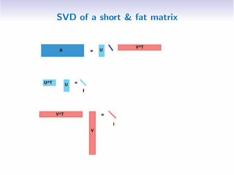
SVD of a short & fat matrix

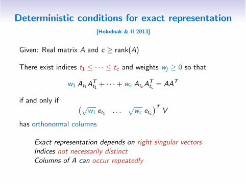
Deterministic conditions for exact representation

[Holodnak & II 2013]

Given: Real matrix A and c ≥ rank(A)

There exist indices t1 ≤ · · · ≤ tc and weights wj ≥ 0 so that

w1 At1ATt1 + · · · + wc AtcA

Ttc = AAT

if and only if(√

w1 et1 . . .√wc etc

)TV

has orthonormal columns

Exact representation depends on right singular vectors

Indices not necessarily distinct

Columns of A can occur repeatedly

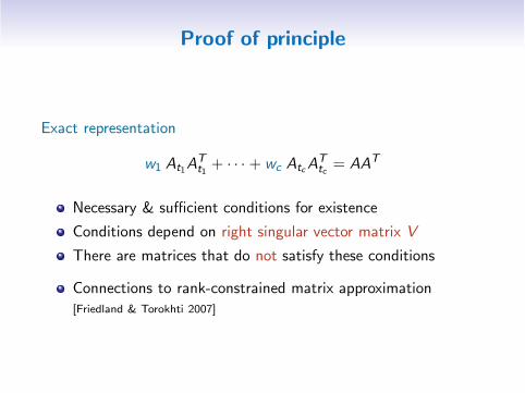
Proof of principle

Exact representation

w1 At1ATt1 + · · · + wc AtcA

Ttc = AAT

Necessary & sufficient conditions for existence

Conditions depend on right singular vector matrix V

There are matrices that do not satisfy these conditions

Connections to rank-constrained matrix approximation[Friedland & Torokhti 2007]

Monte Carlo algorithm

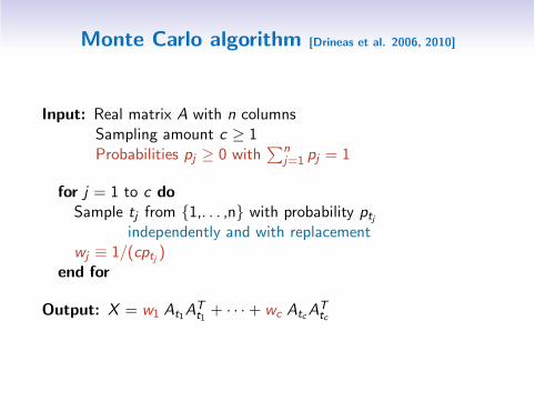
Monte Carlo algorithm [Drineas et al. 2006, 2010]

Input: Real matrix A with n columnsSampling amount c ≥ 1Probabilities pj ≥ 0 with

∑nj=1 pj = 1

for j = 1 to c doSample tj from 1,. . . ,n with probability ptj

independently and with replacementwj ≡ 1/(cptj )

end for

Output: X = w1 At1ATt1 + · · ·+ wc AtcA

Ttc

How to sample

Given: Probabilities 0 ≤ p1 ≤ · · · ≤ pn with∑n

j=1 pj = 1

Want: Sample index t = j from 1,. . . ,n with probability pj

Inversion by sequential search [Devroye 1986]

1 Determine partial sums

Sk ≡k

∑

i=1

pi 1 ≤ k ≤ n

2 Pick uniform [0, 1] random variable U

3 Determine integer j with Sj−1 < U ≤ Sj

4 Sampled index: t = j with probability pj = Sj − Sj−1

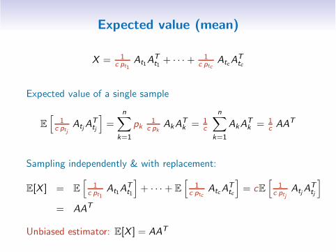
Expected value (mean)

X = 1c pt1

At1ATt1 + · · · + 1

c ptcAtcA

Ttc

Expected value of a single sample

E

[

1c ptj

AtjATtj

]

=

n∑

k=1

pk1

c pkAkA

Tk = 1

c

n∑

k=1

AkATk = 1

c AAT

Sampling independently & with replacement:

E[X ] = E

[

1c pt1

At1ATt1

]

+ · · · + E

[

1c ptc

AtcATtc

]

= cE[

1c ptj

AtjATtj

]

= AAT

Unbiased estimator: E[X ] = AAT

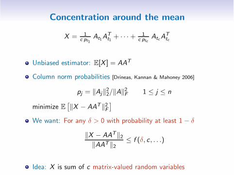
Concentration around the mean

X = 1c pt1

At1ATt1 + · · · + 1

c ptcAtcA

Ttc

Unbiased estimator: E[X ] = AAT

Column norm probabilities [Drineas, Kannan & Mahoney 2006]

pj = ‖Aj‖22/‖A‖2F 1 ≤ j ≤ n

minimize E[

‖X − AAT‖2F]

We want: For any δ > 0 with probability at least 1− δ

‖X − AAT‖2‖AAT‖2

≤ f (δ, c , . . .)

Idea: X is sum of c matrix-valued random variables

8× 4177 Abalone matrix [Bache & Lichman 2013]

0 500 1000 1500 200010− 4

10− 3

10− 2

10− 1

100

Number of Samples (c )

Rela

tive

Err

or

Monte Carlo algorithm has low relative accuracy

Probabilistic bounds

Matrix Bernstein concentration inequality [Tropp 2011]

Independent random real symmetric m ×m matrices Xj

E[Xj ] = 0 zero mean

‖Xj‖2 ≤ τ bounded∥

∥

∥

∑

j E[X2j ]∥

∥

∥

2≤ ρ “variance”

For any ǫ > 0

P

∥

∥

∥

∑

j

Xj

∥

∥

∥

2≥ ǫ

≤ m exp

(

− ǫ2/2

ρ+ τ ǫ/3

)

deviation from the mean

Relative error due to randomization [Holodnak & II]

Given: Real matrix A =(

A1 . . . An

)

Stable rank: sr(A) ≡ ‖A‖2F /‖A‖22Monte Carlo algorithm (with probabilities pj = ‖Aj‖

22/‖A‖

2F )

X = 1c pt1

At1ATt1 + · · · + 1

c ptcAtcA

Ttc

For any δ > 0, with probability at least 1− δ

‖X − AAT‖2‖AAT‖2

≤ γ +√

γ (6 + γ)

where

γ ≡ ln (rank(A)/δ)

3 csr(A)

Lower bound on number of samples [Holodnak & II]

Given: Real matrix A =(

A1 . . . An

)

Monte Carlo algorithm (with probabilities pj = ‖Aj‖22/‖A‖

2F )

X = 1c pt1

At1ATt1 + · · · + 1

c ptcAtcA

Ttc

If 0 < ǫ < 1, 0 < δ < 1 and

c ≥ 83

ln (rank(A)/δ)

ǫ2sr(A)

then with probability at least 1− δ

‖X − AAT‖2‖AAT‖2

≤ ǫ

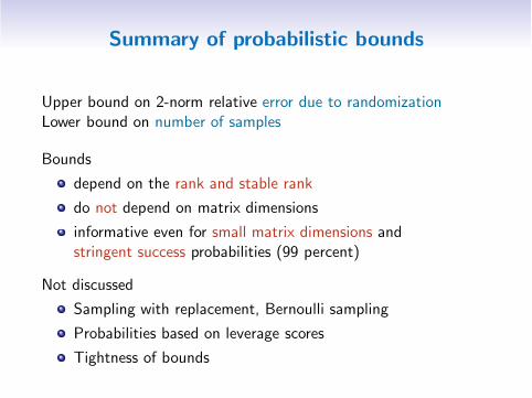
Summary of probabilistic bounds

Upper bound on 2-norm relative error due to randomizationLower bound on number of samples

Bounds

depend on the rank and stable rank

do not depend on matrix dimensions

informative even for small matrix dimensions andstringent success probabilities (99 percent)

Not discussed

Sampling with replacement, Bernoulli sampling

Probabilities based on leverage scores

Tightness of bounds

Special case:Matrices with orthonormal rows

From matrix multiplication to singular values

Given: Real m × n matrix Q with QQT = ImSingular values: σj(Q) = 1, 1 ≤ j ≤ m

Monte Carlo algorithm: X = QQT where Q has c ≥ m columns

‖QQT − I‖2 ≤ ǫ

Matrix multiplication bounds imply singular value bounds

Singular values of Q

√1− ǫ ≤ σj(Q) ≤

√1 + ǫ 1 ≤ j ≤ m

Condition number of Q with respect to inversion

‖Q‖2‖Q†‖2 =σ1(Q)

σm(Q)=

√

1 + ǫ

1− ǫ

Singular value bounds [Holodnak & II]

Given: Real matrix Q =(

Q1 . . . Qn

)

with QQT = Im

Monte Carlo algorithm (with probabilities pj = ‖Qj‖22/m)

X = QQT Q ≡(√

1c pt1

Qt1 . . .√

1c ptc

Qtc

)

If 0 < ǫ < 1, 0 < δ < 1 and

c ≥ 2(1 + ǫ3)m

ln (m/δ)

ǫ2

then with probability at least 1− δ

√1− ǫ ≤ σj(Q) ≤

√1 + ǫ 1 ≤ j ≤ m

Uniform sampling [Holodnak & II]

Given: Real matrix Q =(

Q1 . . . Qn

)

with QQT = Im

Largest column norm µ ≡ max1≤j≤n ‖Qj‖22

Monte Carlo algorithm (with probabilities pj = 1/n)

X = QQT Q ≡(√

1c pt1

Qt1 . . .√

1c ptc

Qtc

)

If 0 < ǫ < 1, 0 < δ < 1 and

c ≥ 2(1 + ǫ3) n µ

ln (m/δ)

ǫ2

then with probability at least 1− δ

√1− ǫ ≤ σj(Q) ≤

√1 + ǫ 1 ≤ j ≤ m

Summary: Matrices with orthonormal rows

Probabilistic singular value bounds

√1− ǫ ≤ σj(Q) ≤

√1 + ǫ 1 ≤ j ≤ m

Column norm probabilities pj = ‖Qj‖22/mNumber of samples c = Ω

(

m lnm/ǫ2)

Uniform probabilities pj = 1/n

Number of samples c = Ω(

nµ lnm/ǫ2)

µ ≡ maxj ‖Qj‖22

Connections to

Coupon collector’s problem (Halko, Martinsson & Tropp)

Compressed sensing (Donoho, Candes, ...)

Coherence

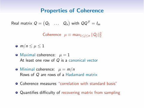
Properties of Coherence

Real matrix Q =(

Q1 . . . Qn

)

with QQT = Im

Coherence µ ≡ max1≤j≤n ‖Qj‖22

m/n ≤ µ ≤ 1

Maximal coherence: µ = 1At least one row of Q is a canonical vector

Minimal coherence: µ = m/nRows of Q are rows of a Hadamard matrix

Coherence measures “correlation with standard basis”

Quantifies difficulty of recovering matrix from sampling

Coherence in General

Donoho & Huo 2001Mutual coherence of two bases

Candes, Romberg & Tao 2006

Candes & Recht 2009Matrix completion: Recovering a low-rank matrix

by sampling its entries

Mori & Talwalkar 2010, 2011

Estimation of coherence

Avron, Maymounkov & Toledo 2010Meng, Saunders & Mahoney 2011

Randomized preconditioners for least squares

Drineas, Magdon-Ismail, Mahoney & Woodruff 2011

Fast approximation of coherence

Leverage scores

Leverage scores

Q =(

Q1 . . . Qn

)

with QQT = Im

Idea: Use all column norms

Leverage scores = squared column norms of Q

ℓj = ‖Qj‖22 1 ≤ j ≤ n

Coherence = largest leverage score

µ = max1≤j≤n

ℓj

Low coherence ⇐⇒ uniform leverage scores

Leverage scores: Importance sampling in randomized algorithms[Drineas & Mahoney 2006, ...]

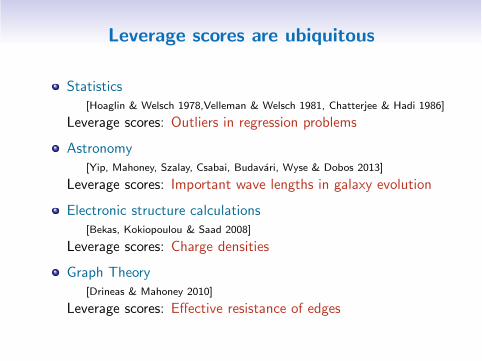
Leverage scores are ubiquitous

Statistics[Hoaglin & Welsch 1978,Velleman & Welsch 1981, Chatterjee & Hadi 1986]

Leverage scores: Outliers in regression problems

Astronomy[Yip, Mahoney, Szalay, Csabai, Budavari, Wyse & Dobos 2013]

Leverage scores: Important wave lengths in galaxy evolution

Electronic structure calculations[Bekas, Kokiopoulou & Saad 2008]

Leverage scores: Charge densities

Graph Theory[Drineas & Mahoney 2010]

Leverage scores: Effective resistance of edges

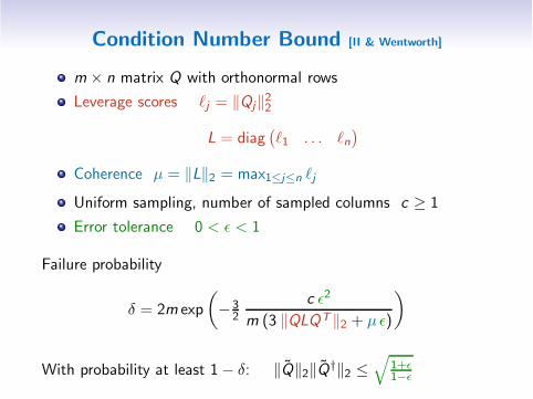
Condition Number Bound [II & Wentworth]

m × n matrix Q with orthonormal rows

Leverage scores ℓj = ‖Qj‖22

L = diag(

ℓ1 . . . ℓn)

Coherence µ = ‖L‖2 = max1≤j≤n ℓj

Uniform sampling, number of sampled columns c ≥ 1

Error tolerance 0 < ǫ < 1

Failure probability

δ = 2m exp

(

−32

c ǫ2

m (3 ‖QLQT ‖2 + µ ǫ)

)

With probability at least 1− δ: ‖Q‖2‖Q†‖2 ≤√

1+ǫ1−ǫ

What to do about ‖QLQT‖2

Failure probability

δ = 2m exp

(

−32

c ǫ2

m (3 ‖QLQT ‖2 + µ ǫ)

)

whereµ2 ≤ ‖QLQT‖2 ≤ µ

Want: Simple accurate approximation of ‖QLQT‖2How: Derive bound for general scaled matrices

Connections toMajorization, lattice superadditive maps

Inverse eigenvalue problems [Dhillon et al. 2005]

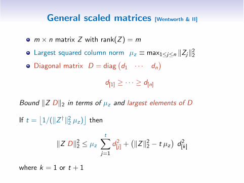
General scaled matrices [Wentworth & II]

m × n matrix Z with rank(Z ) = m

Largest squared column norm µz ≡ max1≤j≤n ‖Zj‖22Diagonal matrix D = diag

(

d1 · · · dn)

d[1] ≥ · · · ≥ d[n]

Bound ‖Z D‖2 in terms of µz and largest elements of D

If t =⌊

1/(‖Z †‖22 µz)⌋

then

‖Z D‖22 ≤ µz

t∑

j=1

d2[j ] +

(

‖Z‖22 − t µz

)

d2[k]

where k = 1 or t + 1

Bound for ‖QLQT‖2

m × n matrix Q with QQT = Im

Coherence µ ≡ max1≤j≤n ‖Qj‖22Leverage scores ℓ[1] ≥ · · · ≥ ℓ[n]

If t = ⌊1/µ⌋ then

‖Q L QT‖2 = ‖Q L1/2‖22 ≤ µ

t∑

j=1

ℓ[j ] + (1− t µ) ℓ[t+1]

If t = 1/µ is an integer then

‖Q L QT‖2 ≤ µt

∑

j=1

ℓ[j ] ≤ µ

Bound for ‖QLQT‖2 tighter than coherence µ

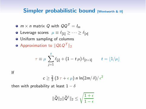
Simpler probabilistic bound [Wentworth & II]

m × n matrix Q with QQT = Im

Leverage scores µ ≡ ℓ[1] ≥ · · · ≥ ℓ[n]

Uniform sampling of columns

Approximation to ‖QLQT ‖2

τ ≡ µ

t∑

j=1

ℓ[j ] + (1− t µ) ℓ[t+1] t = ⌊1/µ⌋

Ifc ≥ 2

3 (3 τ + ǫ µ) n ln(2m/ δ)/ ǫ2

then with probability at least 1− δ

‖Q‖2‖Q†‖2 ≤√

1 + ǫ

1− ǫ

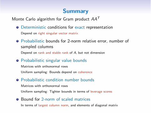
Summary

Monte Carlo algorithm for Gram product AAT

Deterministic conditions for exact representationDepend on right singular vector matrix

Probabilistic bounds for 2-norm relative error, number ofsampled columnsDepend on rank and stable rank of A, but not dimension

Probabilistic singular value boundsMatrices with orthonormal rows

Uniform sampling: Bounds depend on coherence

Probabilistic condition number boundsMatrices with orthonormal rows

Uniform sampling: Tighter bounds in terms of leverage scores

Bound for 2-norm of scaled matricesIn terms of largest column norm, and elements of diagonal matrix

Why randomized algorithms?

Reduction of massive data sets, for low-accuracy requirementsLeast squares/regression, SVD/PCA, subspace approximation, model reduction

Advantages“Easy” to analyze, forgiving, probabilistic bounds more optimistic

ApplicationsMachine learning, population genomics, astronomy, nuclear engineering

Survey papers

Halko, Martinsson & Tropp 2011Mahoney 2011