introduction to queueing theory - washington …jain/queue/ftp/q_30iqt.pdf · 30-1 uc berkeley,...

30-1©2012 Raj JainUC Berkeley, Fall 2012

Introduction to Introduction to Queueing TheoryQueueing Theory

Raj JainWashington University in Saint Louis

[email protected] or [email protected] Mini-Course offered at UC Berkeley, Sept-Oct 2012

These slides and audio/video recordings are available on-line at:http://amplab.cs.berkeley.edu/courses/queueand http://www.cse.wustl.edu/~jain/queue


OverviewOverview

Queueing Notation Rules for All Queues Little's Law Types of Stochastic Processes


Basic Components of a QueueBasic Components of a Queue

1. Arrivalprocess

6. Servicediscipline

2. Service timedistribution

4. Waiting positions 3. Number of

servers

5. Population Size


Kendall Notation Kendall Notation A/S/m/B/K/SDA/S/m/B/K/SD A: Arrival process S: Service time distribution m: Number of servers B: Number of buffers (system capacity) K: Population size, and SD: Service discipline


Arrival ProcessArrival Process Arrival times: Interarrival times: j form a sequence of Independent and Identically Distributed

(IID) random variables Notation:

M = Memoryless Exponential E = Erlang H = Hyper-exponential D = Deterministic constant G = General Results valid for all distributions


Service Time DistributionService Time Distribution Time each student spends at the terminal. Service times are IID. Distribution: M, E, H, D, or G Device = Service center = Queue Buffer = Waiting positions


Service DisciplinesService Disciplines First-Come-First-Served (FCFS) Last-Come-First-Served (LCFS) = Stack (used in 9-1-1 calls) Last-Come-First-Served with Preempt and Resume (LCFS-PR) Round-Robin (RR) with a fixed quantum. Small Quantum Processor Sharing (PS) Infinite Server: (IS) = fixed delay Shortest Processing Time first (SPT) Shortest Remaining Processing Time first (SRPT) Shortest Expected Processing Time first (SEPT) Shortest Expected Remaining Processing Time first (SERPT). Biggest-In-First-Served (BIFS) Loudest-Voice-First-Served (LVFS)


Example Example M/M/3/20/1500/FCFSM/M/3/20/1500/FCFS Time between successive arrivals is exponentially distributed. Service times are exponentially distributed. Three servers 20 Buffers = 3 service + 17 waiting After 20, all arriving jobs are lost Total of 1500 jobs that can be serviced. Service discipline is first-come-first-served. Defaults:

Infinite buffer capacity Infinite population size FCFS service discipline.

G/G/1 = G/G/1/∞/∞/FCFS


Quiz 30AQuiz 30A

Key: A/S/m/B/K/SDT F The number of servers in a M/M/1/3 queue is 3 G/G/1/30/300/LCFS queue is like a stack M/D/3/30 queue has 30 buffers G/G/1 queue has ∞ population size D/D/1 queue has FCFS discipline


Exponential DistributionExponential Distribution Probability Density Function (pdf):

Cumulative Distribution Function (cdf):

Mean: a

Variance: a2

Coefficient of Variation = (Std Deviation)/mean = 1 Memoryless:

Expected time to the next arrival is always a regardless of the time since the last arrival

Remembering the past history does not help.

f(x) =1

ae−x/a

F (x) = P (X < x) =

Z x

0

f(x)dx = 1− e−x/ax

f(x)

x

F(x)

1a

1


ErlangErlang DistributionDistribution Sum of k exponential random variables

Series of k servers with exponential service times

Probability Density Function (pdf):

Expected Value: ak Variance: a2k CoV: 1/k

f(x) =xk−1e−x/a

(k − 1)!ak

X =

kXi=1

xi where xi ∼ exponential

1 k…


HyperHyper--Exponential DistributionExponential Distribution The variable takes ith value with probability pi

xi is exponentially distributed with mean ai

Higher variance than exponentialCoefficient of variation > 1

x1

x2

xm

x…


Group Arrivals/ServiceGroup Arrivals/Service Bulk arrivals/service M[x]: x represents the group size G[x]: a bulk arrival or service process with general inter-group

times. Examples:

M[x]/M/1 : Single server queue with bulk Poisson arrivals and exponential service times

M/G[x]/m: Poisson arrival process, bulk service with general service time distribution, and m servers.


Quiz 30BQuiz 30B

Exponential distribution is denoted as ___ ____________ distribution represents a set of parallel

exponential servers Erlang distribution Ek with k=1 is same as ________

distribution


Key VariablesKey Variables1

2

m

PreviousArrival Arrival

BeginService

EndService

w sr

nnq ns

Time


Key Variables (cont)Key Variables (cont) Inter-arrival time = time between two successive arrivals. Mean arrival rate = 1/E[]

May be a function of the state of the system, e.g., number of jobs already in the system.

s = Service time per job. = Mean service rate per server = 1/E[s] Total service rate for m servers is m n = Number of jobs in the system.

This is also called queue length. Note: Queue length includes jobs currently receiving service

as well as those waiting in the queue.


Key Variables (cont)Key Variables (cont) nq = Number of jobs waiting ns = Number of jobs receiving service r = Response time or the time in the system

= time waiting + time receiving service w = Waiting time

= Time between arrival and beginning of service


Rules for All QueuesRules for All QueuesRules: The following apply to G/G/m queues1. Stability Condition: Arrival rate must be less than service rate

< mFinite-population or finite-buffer systems are always stable. Instability = infinite queueSufficient but not necessary. D/D/1 queue is stable at λ=μ

2. Number in System versus Number in Queue:n = nq+ nsNotice that n, nq, and ns are random variables. E[n]=E[nq]+E[ns]If the service rate is independent of the number in the queue, Cov(nq,ns) = 0


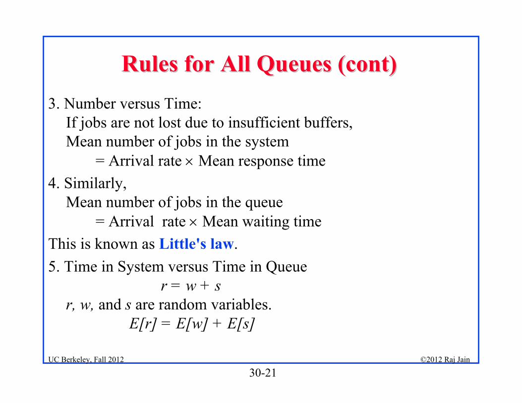
Rules for All Queues (cont)Rules for All Queues (cont)3. Number versus Time:

If jobs are not lost due to insufficient buffers, Mean number of jobs in the system

= Arrival rate Mean response time4. Similarly,

Mean number of jobs in the queue = Arrival rate Mean waiting time

This is known as Little's law.5. Time in System versus Time in Queue

r = w + sr, w, and s are random variables.

E[r] = E[w] + E[s]


Rules for All Queues(cont)Rules for All Queues(cont)6. If the service rate is independent of the number of jobs in the

queue, Cov(w,s)=0


Quiz 30CQuiz 30C

If a queue has 2 persons waiting for service, the number is system is ____

If the arrival rate is 2 jobs/second, the mean inter-arrival time is _____ second.

In a 3 server queue, the jobs arrive at the rate of 1 jobs/second, the service time should be less than ____ second/job for the queue to be stable.


Little's LawLittle's Law Mean number in the system

= Arrival rate Mean response time This relationship applies to all systems or parts of systems in

which the number of jobs entering the system is equal to those completing service.

Named after Little (1961) Based on a black-box view of the system:

In systems in which some jobs are lost due to finite buffers, the law can be applied to the part of the system consisting of the waiting and serving positions

BlackBox

Arrivals Departures


Proof of Little's LawProof of Little's Law

If T is large, arrivals = departures = N Arrival rate = Total arrivals/Total time= N/T Hatched areas = total time spent inside the

system by all jobs = J Mean time in the system= J/N Mean Number in the system

= J/T = = Arrival rate× Mean time in the system

1 2 3 4 5 6 7 8

1234

Jobnumber

Arrival

Departure

1 2 3 4 5 6 7 8

1234

Numberin

System

Time Time

1 2 3

1234

Timein

System

Job number


Application of Little's LawApplication of Little's Law

Applying to just the waiting facility of a service center Mean number in the queue = Arrival rate Mean waiting time Similarly, for those currently receiving the service, we have: Mean number in service = Arrival rate Mean service time

Arrivals Departures


Example 30.3Example 30.3 A monitor on a disk server showed that the average time to

satisfy an I/O request was 100 milliseconds. The I/O rate was about 100 requests per second. What was the mean number of requests at the disk server?

Using Little's law:Mean number in the disk server= Arrival rate Response time= 100 (requests/second) (0.1 seconds)= 10 requests


Quiz 30DQuiz 30D

Key: n = λ R During a 1 minute observation, a server received 120

requests. The mean response time was 1 second. The mean number of queries in the server is _____


Stochastic ProcessesStochastic Processes Process: Function of time Stochastic Process: Random variables, which are functions of

time Example 1:

n(t) = number of jobs at the CPU of a computer system Take several identical systems and observe n(t) The number n(t) is a random variable. Can find the probability distribution functions for n(t) at

each possible value of t. Example 2:

w(t) = waiting time in a queue


Types of Stochastic ProcessesTypes of Stochastic Processes Discrete or Continuous State Processes Markov Processes Birth-death Processes Poisson Processes


Discrete/Continuous State ProcessesDiscrete/Continuous State Processes Discrete = Finite or Countable Number of jobs in a system n(t) = 0, 1, 2, .... n(t) is a discrete state process The waiting time w(t) is a continuous state process. Stochastic Chain: discrete state stochastic process Note: Time can also be discrete or continuous

Discrete/continuous time processesHere we will consider only continuous time processes

State

Time


Markov ProcessesMarkov Processes Future states are independent of the past and depend only on

the present. Named after A. A. Markov who defined and analyzed them in

1907. Markov Chain: discrete state Markov process Markov It is not necessary to history of the previous states

of the process Future depends upon the current state only M/M/m queues can be modeled using Markov processes. The time spent by a job in such a queue is a Markov process

and the number of jobs in the queue is a Markov chain.


BirthBirth--Death ProcessesDeath Processes

The discrete space Markov processes in which the transitions are restricted to neighboring states

Process in state n can change only to state n+1 or n-1. Example: the number of jobs in a queue with a single server

and individual arrivals (not bulk arrivals)

0 1 2 j-1 j j+1… j j j

j j j


Poisson DistributionPoisson Distribution If the inter-arrival times are exponentially distributed,

number of arrivals in any given interval are Poisson distributed

M = Memoryless arrival = Poisson arrivals Example: λ=4 4 jobs/sec or 0.25 sec between jobs on average

τ ~ Exponentialtime

n ~ Poisson

f(τ) = λe−λτ E[τ ] = 1λ

P (n arrivals in t) = (λt)n e−λt

n! E[n] = λt


Poisson ProcessesPoisson Processes Interarrival time s = IID and exponential

number of arrivals n over a given interval (t, t+x) has a Poisson distribution arrival = Poisson process or Poisson stream

Properties: 1.Merging:

2.Splitting: If the probability of a job going to ithsubstream is pi, each substream is also Poisson with a mean rate of pi


Poisson Processes (Cont)Poisson Processes (Cont)

3.If the arrivals to a single server with exponential service time are Poisson with mean rate , the departures are also Poisson with the same rate provided < .


Poisson Process(cont)Poisson Process(cont) 4. If the arrivals to a service facility with m service centers

are Poisson with a mean rate , the departures also constitute a Poisson stream with the same rate , provided < i i. Here, the servers are assumed to have exponentially distributed service times.


PASTA PropertyPASTA Property Poisson Arrivals See Time Averages Poisson arrivals Random arrivals from a large number of

independent sources If an external observer samples a system at a random instant:

P(System state = x) = P(State as seen by a Poisson arrival is x)Example: D/D/1 Queue: Arrivals = 1 job/sec, Service =2 jobs/sec

All customers see an empty system. M/D/1 Queue: Arrivals = 1 job/sec (avg), Service = 2 jobs/sec

Randomly sample the system. System is busy half of the time.

0 1 2 3 4 5

0 1 2 3 4 5


Relationship Among Stochastic ProcessesRelationship Among Stochastic Processes


Quiz 30EQuiz 30E

T F Birth-death process can have bulk service Merger of Poisson processes results in a _______

Process The number of jobs in a M/M/1 queue is Markov

______ T F A discrete time process is also called a chain


SummarySummary

Kendall Notation: A/S/m/B/k/SD, M/M/1 Number in system, queue, waiting, service

Service rate, arrival rate, response time, waiting time, servicetime

Little’s Law: Mean number in system = Arrival rate ×Mean time in system

Processes: Markov Only one state required, Birth-death Adjacent states Poisson IID and exponential inter-arrival


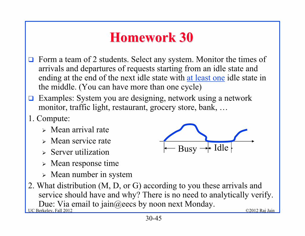
Homework 30Homework 30 Form a team of 2 students. Select any system. Monitor the times of

arrivals and departures of requests starting from an idle state and ending at the end of the next idle state with at least one idle state in the middle. (You can have more than one cycle)

Examples: System you are designing, network using a network monitor, traffic light, restaurant, grocery store, bank, …

1. Compute: Mean arrival rate Mean service rate Server utilization Mean response time Mean number in system

2. What distribution (M, D, or G) according to you these arrivals and service should have and why? There is no need to analytically verify.Due: Via email to jain@eecs by noon next Monday.

Busy Idle


Reading ListReading List

If you need to refresh your probability concepts, read chapter 12

Read Chapter 30 Refer to Chapter 29 for various distributions

introduction to queueing theory - washington …jain/queue/ftp/q_30iqt.pdf · 30-1 uc berkeley,...

Documents