Introduction to Quantitative Genetics

Quantitative Characteristics Many traits in humans and other organisms are genetically

influenced, but do not show single-gene (Mendelian) patterns of inheritance.

They are influenced by the combined action of many genes and are characterized by continuous variation. These are

called polygenic traits.

Continuously variable characteristics that are both polygenic and influenced by environmental factors are called

multifactorial traits. Examples of quantitative characteristics are height, intelligence & hair color.

Types of Quantitative Traits

1. a continues measurement (quantity).

2. a countable meristic (measured in whole numbers). It can take on integer values only: For example, litter size.

3. a threshold characteristic which is either present or absent depending on the cumulative effect of a number of additive factors (diseases are often this type). It has an underlying quantitative distribution, but the trait only appears only if a

threshold is crossed.

Types of Quantitative Trait

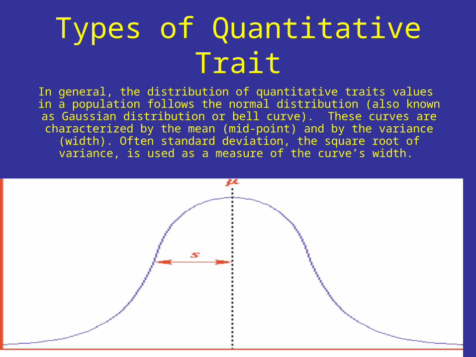
In general, the distribution of quantitative traits values in a population follows the normal distribution (also known as Gaussian distribution or bell curve).

These curves are characterized by the mean (mid-point) and by the variance (width). Often standard deviation, the square root of variance, is used as a

measure of the curve’s width.

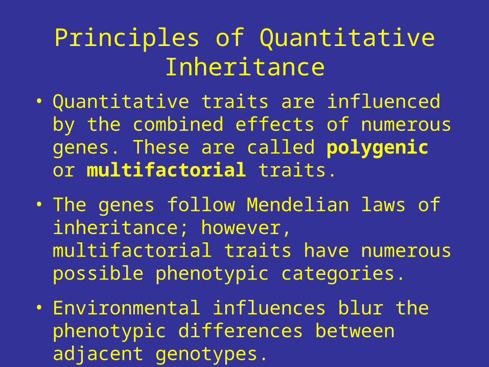
Principles of Quantitative Inheritance

• Quantitative traits are influenced by the combined effects of numerous genes. These are called polygenic or multifactorial traits.

• The genes follow Mendelian laws of inheritance; however, multifactorial traits have numerous possible phenotypic categories.

• Environmental influences blur the phenotypic differences between adjacent genotypes.

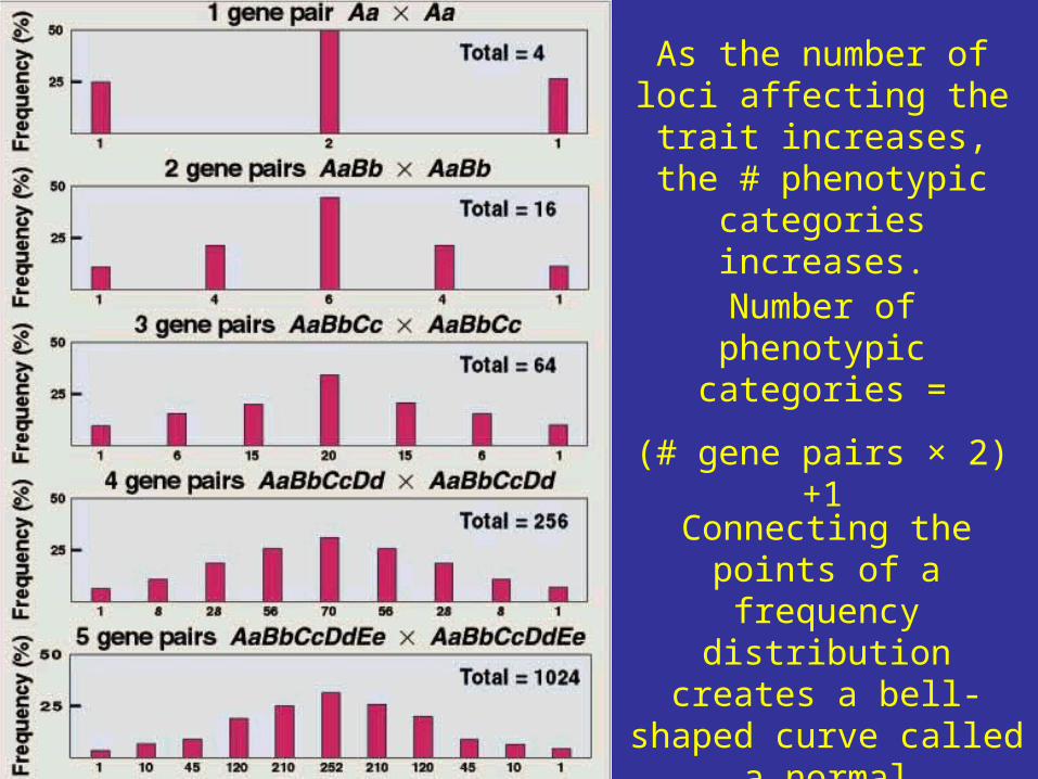
Number of phenotypic categories =

(# gene pairs × 2) +1

Connecting the points of a frequency distribution creates a

bell-shaped curve called a normal distribution.

As the number of loci affecting the trait increases, the # phenotypic categories

increases.

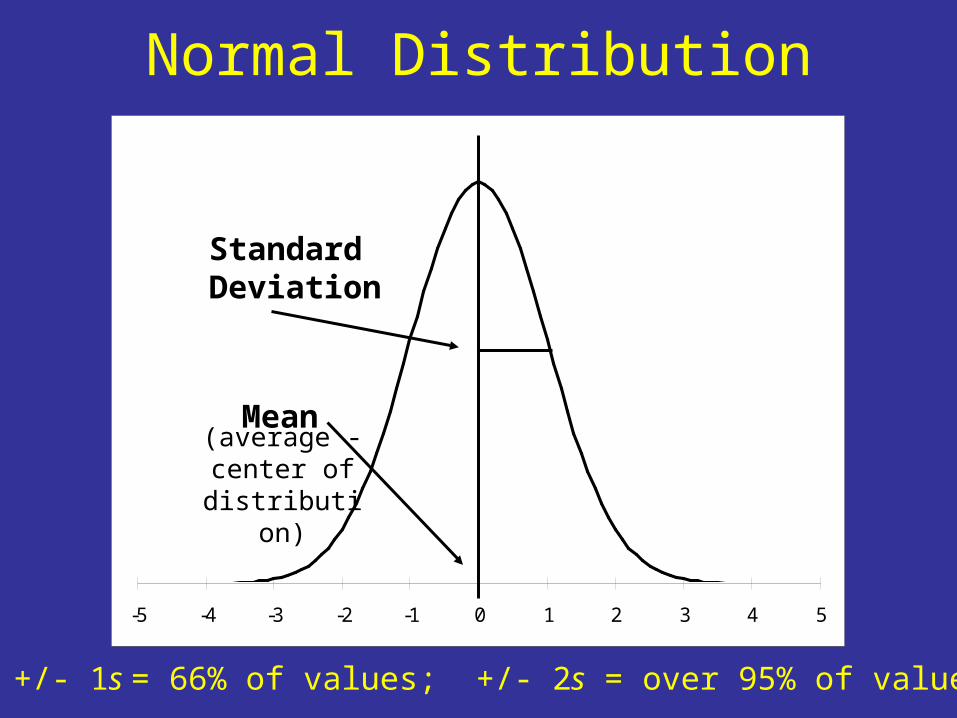
-5 -4 -3 -2 -1 0 1 2 3 4 5

Normal Distribution

StandardDeviation

Mean

Mean +/- 1s = 66% of values; +/- 2s = over 95% of values

(average -center of

distribution)

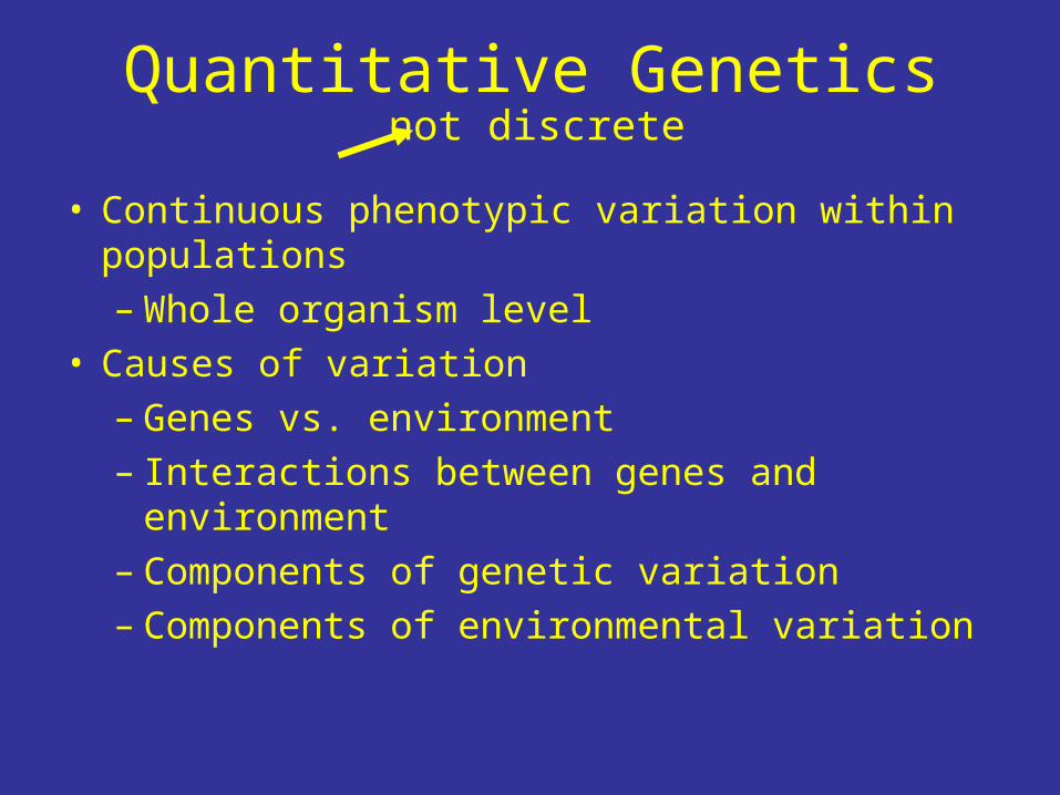
Quantitative Genetics

• Continuous phenotypic variation within populations– Whole organism level

• Causes of variation– Genes vs. environment– Interactions between genes and environment– Components of genetic variation– Components of environmental variation

not discrete

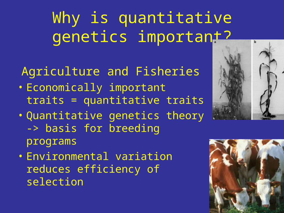
Why is quantitative genetics important?

Agriculture and Fisheries• Economically important traits =

quantitative traits• Quantitative genetics theory -> basis

for breeding programs• Environmental variation reduces

efficiency of selection

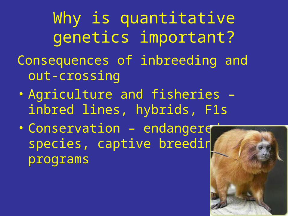
Why is quantitative genetics important?

Consequences of inbreeding and out-crossing• Agriculture and fisheries – inbred lines, hybrids, F1s• Conservation – endangered species, captive

breeding programs

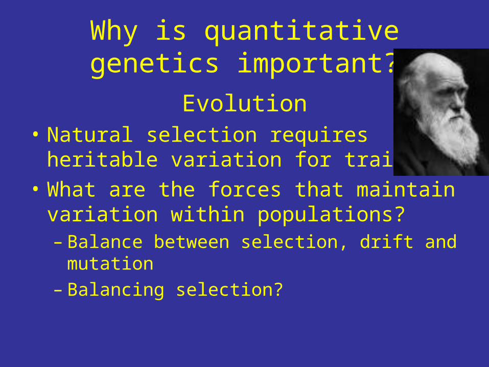
Why is quantitative genetics important?

Evolution• Natural selection requires heritable variation for

traits• What are the forces that maintain variation within

populations?– Balance between selection, drift and mutation– Balancing selection?

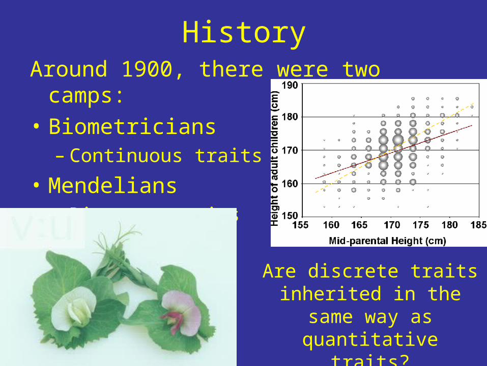
HistoryAround 1900, there were two camps:• Biometricians

– Continuous traits• Mendelians

– Discrete traits

Are discrete traits inherited in the same way as quantitative

traits?

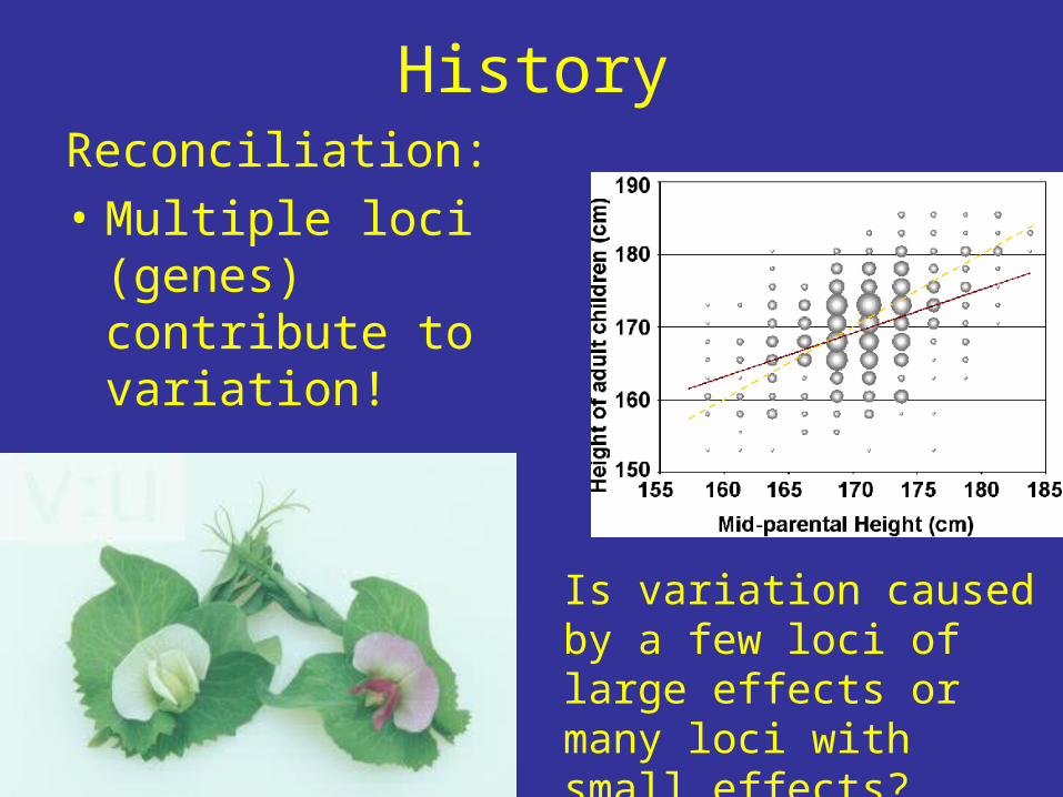
HistoryReconciliation:• Multiple loci

(genes) contribute to variation!

Is variation caused by a few loci of large effects or many loci with small effects?

Mathematical Basis of Quantitative Genetics

• The basic premise of quantitative genetics: phenotype = genetics plus environment.

P = G + E• In fact we are looking at variation in the traits, which is

measured by the width of the Gaussian distribution curve. This width is the variance (or its square root, the standard deviation).

• Variance is a useful property, because variances from different sources can be added together to get total variance.

Mathematical Basis of Quantitative Genetics

• Quantitative traits can thus be expressed as: VT = VG + VE

where VT = total variance, VG - variance due to genetics, and VE = variance due to environmental (non-inherited) causes.

• This equation is often written with an additional covariance term: the degree to which genetic and environmental variance depend on each other. We are just going to assume this term equals zero in our discussions.

Heritability

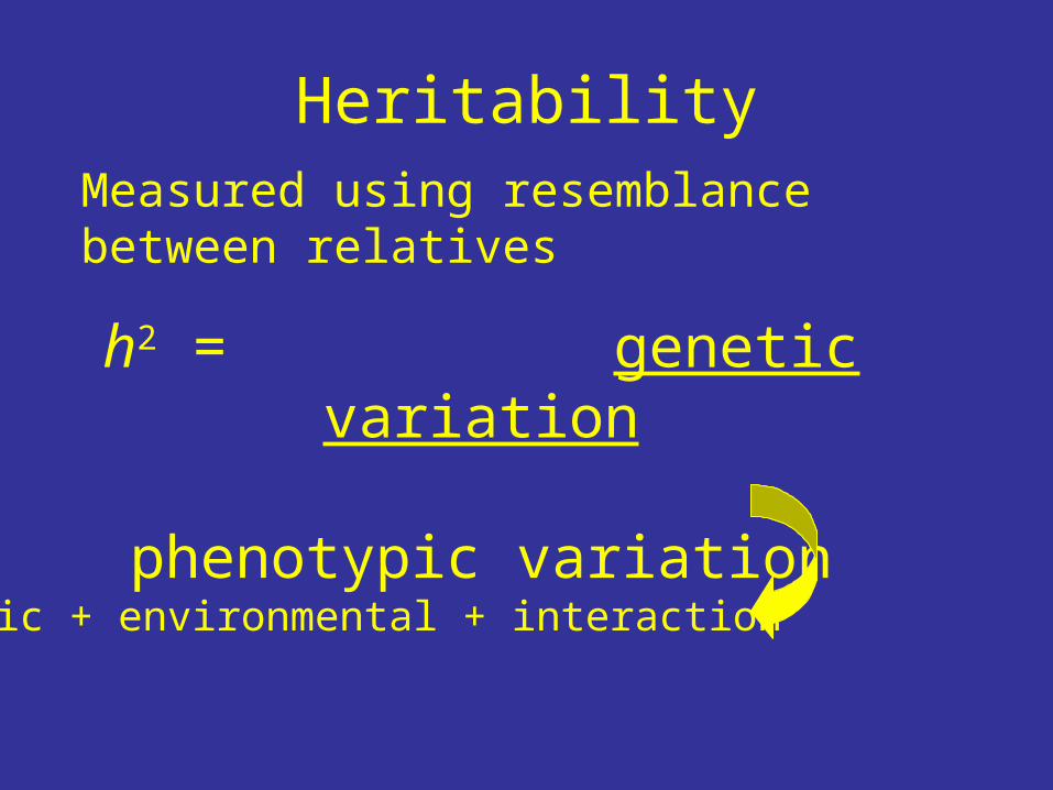
h2 = genetic variation phenotypic variation

Measured using resemblance between relatives

Genetic + environmental + interaction

Heritability One property of interest is “heritability”, the proportion of a trait’s variation that

is due to genetics (with the rest of it due to “environmental” factors). This seems like a simple concept, but it is loaded with problems.

The broad-sense heritability, symbolized as H (sometimes H2 to indicate that the units of variance are squared). H is a simple translation of the statement

from above into mathematics: H = VG / VT

This measure, the broad-sense heritability, is fairly easy to measure, especially in human populations where identical twins are available.

However, different studies show wide variations in H values for the same traits, and plant breeders have found that it doesn’t accurately reflect the results of selection experiments. Thus, H is generally only used in social

science work.

Heritability(broad-sense)

Heritability (broad-sense) is the proportion of a population’s phenotypic variance that is attributable

to genetic differences

Genetic Variance

The biggest problem with broad sense heritability comes from lumping all genetic phenomena into a single Vg factor.

Paradoxically, not all variation due to genetic differences can be directly inherited by an offspring from the parents.

Genetic variance can be split into 2 main components, additive genetic variance (VA) and dominance genetic variance (VD).

VG = VA + VD

Additive variance is the variance in a trait that is due to the effects of each individual allele being added together, without any

interactions with other alleles or genes.

Additive vs. Dominance Genetic Variance

Dominance variance is the variance that is due to interactions between alleles: synergy, effects due to two alleles interacting to make the trait greater (or lesser) than the sum of the two alleles acting alone. We are using dominance variance to include both interactions between alleles of the same gene and interactions

between difference genes, which is sometimes a separate component called epistasis variance.

The important point: dominance variance is not directly inherited from parent to offspring. It is due to the interaction of genes from both parents within the individual, and of course only one allele is

passed from each parent to the offspring.

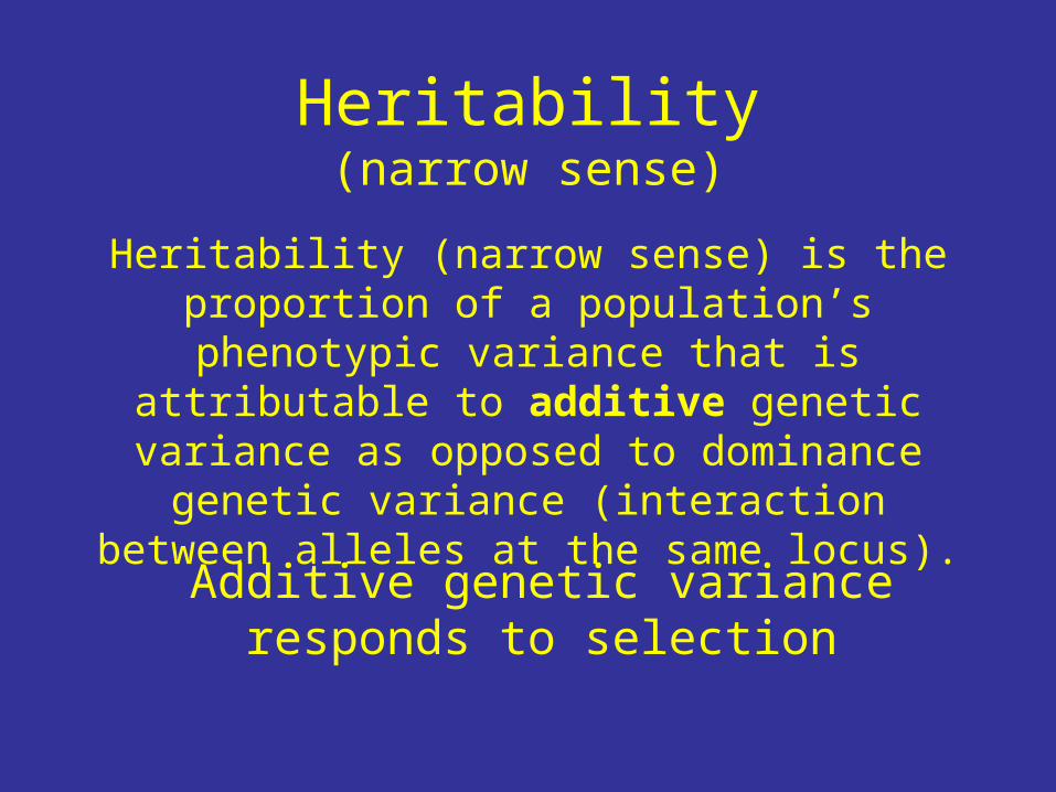
Heritability(narrow sense)

Heritability (narrow sense) is the proportion of a population’s phenotypic variance that is attributable to additive genetic

variance as opposed to dominance genetic variance (interaction between alleles at the same locus).

Additive genetic variance responds to selection

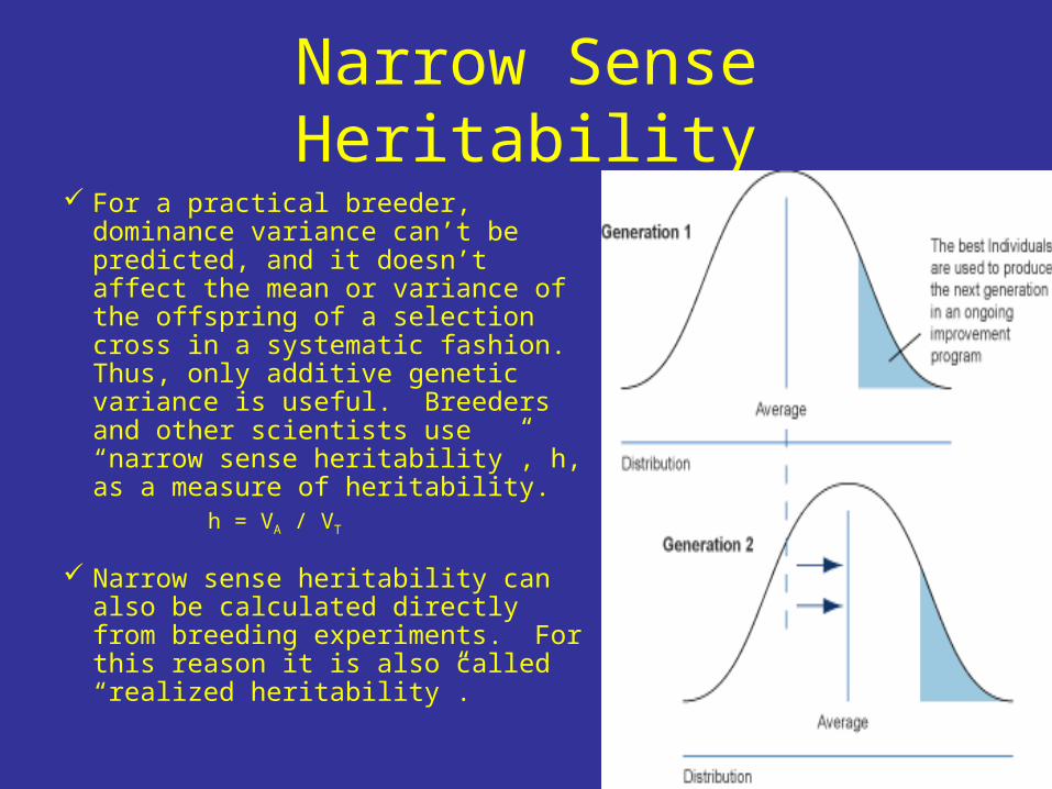
Narrow Sense Heritability For a practical breeder, dominance

variance can’t be predicted, and it doesn’t affect the mean or variance of the offspring of a selection cross in a systematic fashion. Thus, only additive genetic variance is useful. Breeders and other scientists use “narrow sense heritability”, h, as a measure of heritability.

h = VA / VT

Narrow sense heritability can also be calculated directly from breeding experiments. For this reason it is also called “realized heritability”.

The genetic Correlation

Traits are not inherited as independent unit, but the several traits tend to be associated with each other

This phenomenon can arise in 2 ways:

1. A subset of the genes that influence one trait may also influence another trait (pleiotropy)

2. The genes may act independently on the two traits, but due to non random mating, selection, or drift, they may be associated (linkage

disequilibrium)

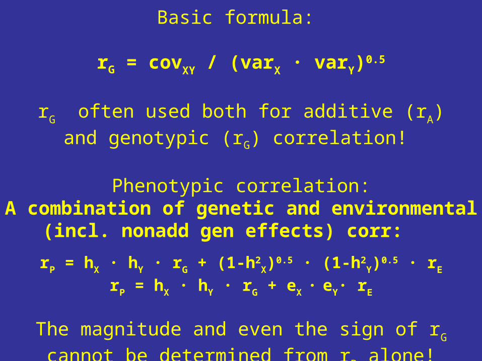
 Basic formula:

rG = covXY / (varX ∙ varY)0.5

rG often used both for additive (rA)and genotypic (rG) correlation!

Phenotypic correlation:

A combination of genetic and environmental (incl. nonadd gen effects) corr:

rP = hX ∙ hY ∙ rG + (1-h2X)

0.5 ∙ (1-h2Y)

0.5 ∙ rE

rP = hX ∙ hY ∙ rG + eX ∙ eY∙ rE

The magnitude and even the sign of rG cannot be determined from rP alone!

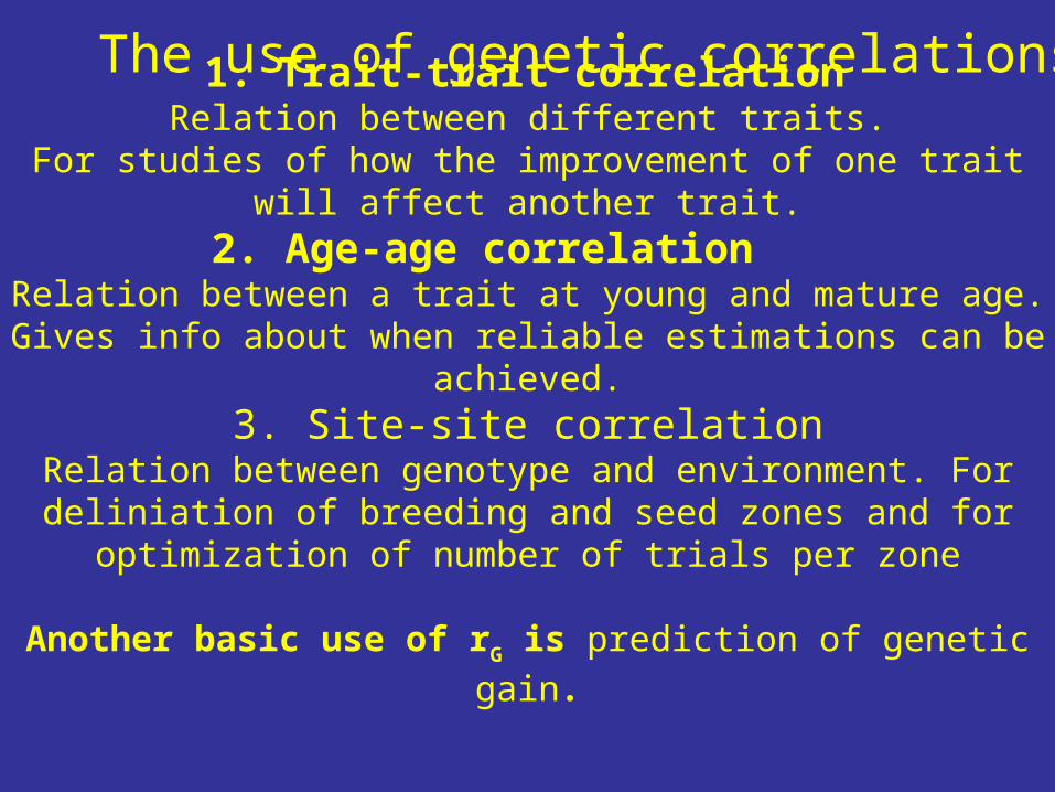
1. Trait-trait correlationRelation between different traits.

For studies of how the improvement of one trait will affect another trait.2. Age-age correlation

Relation between a trait at young and mature age. Gives info about when reliable estimations can be achieved.

3. Site-site correlationRelation between genotype and environment. For deliniation of breeding and

seed zones and for optimization of number of trials per zone

Another basic use of rG is prediction of genetic gain.

The use of genetic correlations

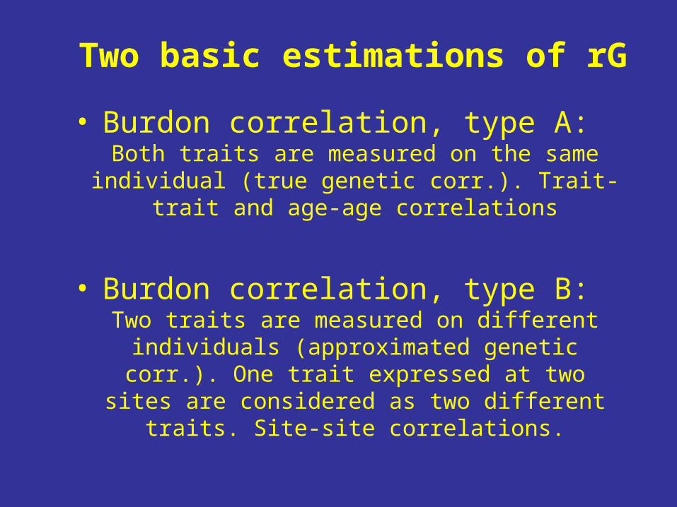
• Burdon correlation, type A: Both traits are measured on the same individual (true genetic

corr.). Trait-trait and age-age correlations

• Burdon correlation, type B:

Two traits are measured on different individuals (approximated genetic corr.). One trait expressed at two sites are considered as

two different traits. Site-site correlations.

Two basic estimations of rG

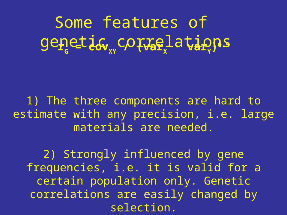
rG = covXY / (varX ∙ varY)0.5

1) The three components are hard to estimate with any precision, i.e.

large materials are needed.

2) Strongly influenced by gene frequencies, i.e. it is valid for a certain population only. Genetic correlations are easily changed by selection.

.

Some features of genetic correlations

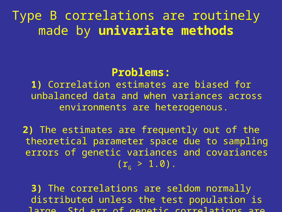
Problems:1) Correlation estimates are biased for unbalanced data and when variances

across environments are heterogenous.

2) The estimates are frequently out of the theoretical parameter space due to sampling errors of genetic variances and covariances (rG > 1.0).

3) The correlations are seldom normally distributed unless the test population is large. Std err of genetic correlations are difficult to estimate and are often approximated! Estimates of std err. should be interpreted

with caution. However they indicate the relatively reliability

Type B correlations are routinely made by univariate methods

 

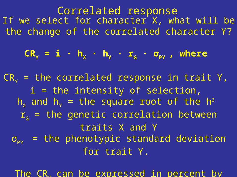
If we select for character X, what will be the change of the correlated

character Y?

CRY = i ∙ hX ∙ hY ∙ rG ∙ σPY , where

CRY = the correlated response in trait Y, i = the intensity of selection,

hX and hY = the square root of the h2 rG = the genetic correlation between traits X and YσPY = the phenotypic standard deviation for trait Y.

The CRY can be expressed in percent by relating it to the phenotypic

mean of variable Y.

Correlated response

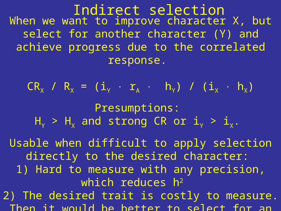
When we want to improve character X, but select for another character (Y) and achieve progress due to the correlated response.

CRX / RX = (iY ∙ rA ∙ hY) / (iX ∙ hX)

Presumptions: HY > HX and strong CR or iY > iX.

Usable when difficult to apply selection directly to the desired character:

1) Hard to measure with any precision, which reduces h2 2) The desired trait is costly to measure. Then it would be better to

select for an easily measurable, correlated trait.

Indirect selection

1 2

1 2

1 2

1 2

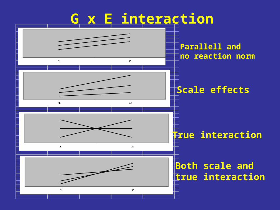
Parallell andno reaction norm

Scale effects

True interaction

Both scale andtrue interaction

G x E interaction

 

It is the ”true interactions” that should affect breeding strategies. Scale effects can be handled by transformation prior to analysis to

ensure homogenity of among-genotype variances in environments. The question is whether breeding should be producing genotypes

suitable for specific environments or genotypes adapted to a wide range of environments?

G x E can be used in practice when interactions and the specific environments are well defined.

The smaller G x E, the fewer test sites are needed.

G x E interaction

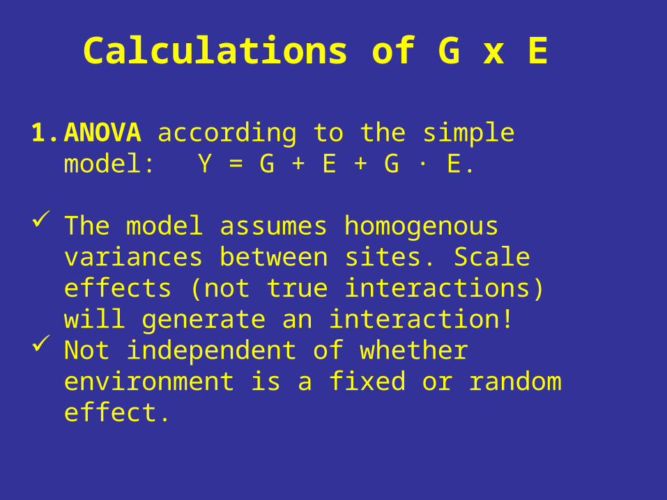
Calculations of G x E

1. ANOVA according to the simple model: Y = G + E + G ∙ E.

The model assumes homogenous variances between sites. Scale effects (not true interactions) will generate an interaction!

Not independent of whether environment is a fixed or random effect.

 

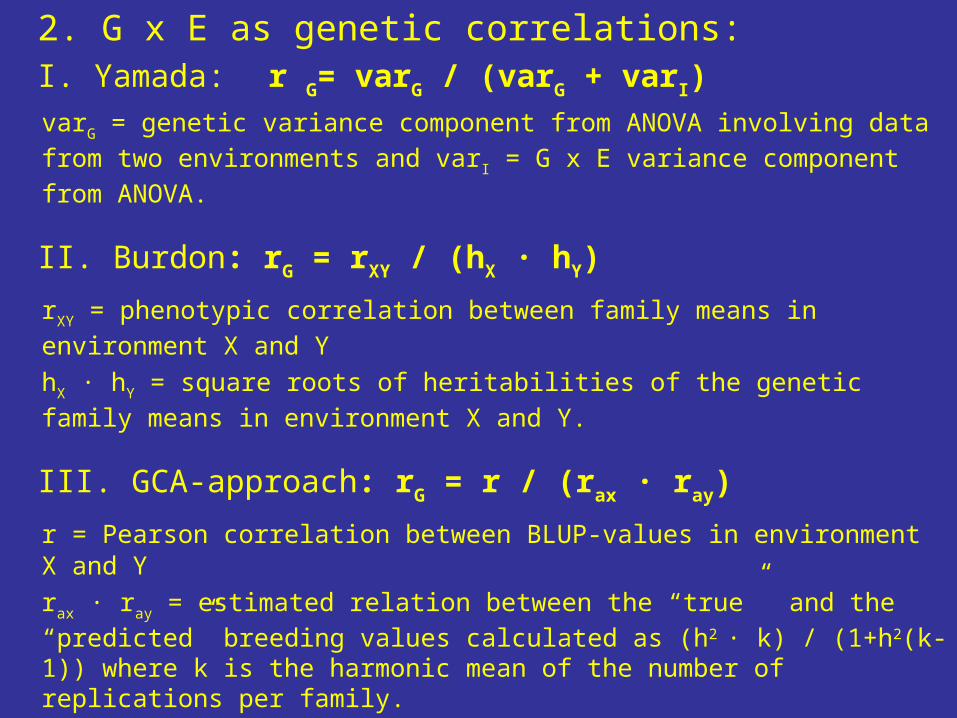
2. G x E as genetic correlations:I. Yamada: r G= varG / (varG + varI) varG = genetic variance component from ANOVA involving data from two environments and varI = G x E variance component from ANOVA.

II. Burdon: rG = rXY / (hX ∙ hY)

rXY = phenotypic correlation between family means in environment X and Y

hX ∙ hY = square roots of heritabilities of the genetic family means in environment X and Y.

III. GCA-approach: rG = r / (rax ∙ ray)

r = Pearson correlation between BLUP-values in environment X and Yrax ∙ ray = estimated relation between the “true” and the “predicted” breeding values calculated as (h2 ∙ k) / (1+h2(k-1)) where k is the harmonic mean of the number of replications per family.

HeterosisBoth the parental lines and the F1’s are genetically uniform.

However, the parental lines are relatively small and weak, a phenomenon called “inbreeding depression”: Too much

homozygosity leads to small, sickly and weak organisms, at least among organisms that usually breed with others

instead of self-pollinating. In contrast, the F1 hybrids are large, healthy and strong.

This phenomenon is called “heterosis” or “hybrid vigor”. The corn planted in the US and other developed countries

in nearly all F1 hybrid seed, because it produces high yielding, healthy plants (due to heterosis) and it is

genetically uniform (and thus matures at the same time with ears in the same position on every plant).